Three dimensional image restoration in ﬂuorescence ... · Three dimensional image restoration in...

Three dimensional image restoration in fluorescencelifetime imaging microscopy

A. SQUIRE & P. I. H. BASTIAENSCell Biophysics Laboratory, Imperial Cancer Research Fund, 44 Lincoln’s Inn Fields, London,WC2A 3PX, U.K.

Key words. Deblurring, deconvolution, FLIM, GFP, green fluorescent protein,ICTM, image processing, MCP, PSF, regularization.

Summary

A microscope set-up and numerical methods are describedwhich enable the measurement and reconstruction ofthree-dimensional nanosecond fluorescence lifetime imagesin every voxel. The frequency domain fluorescence lifetimeimaging microscope (FLIM) utilizes phase detection of high-frequency modulated light by homodyne mixing on amicrochannel plate image intensifier. The output signal atthe image intensifier’s phosphor screen is integrated on acharge coupled device camera. A scanning stage isemployed to obtain a series of phase-dependent intensityimages at equally separated depths in a specimen. TheFourier transform of phase-dependent data gives three-dimensional (3D) images of the Fourier coefficients. Theseimages are deblurred using an Iterative ConstrainedTikhonov–Miller (ICTM) algorithm in conjunction with ameasured point spread function. The 3D reconstruction offluorescence lifetimes are calculated from the deblurredimages of the Fourier coefficients. An improved spatial andtemporal resolution of fluorescence lifetimes was obtainedusing this approach to the reconstruction of simulated 3DFLIM data. The technique was applied to restore 3D FLIMdata of a live cell specimen expressing two green fluorescentprotein fusion constructs having distinct fluorescencelifetimes which localized to separate cellular compartments.

Introduction

The fluorescence lifetime of a fluorophore is a sensitiveparameter for excited state reactions such as fluorescenceresonance energy transfer or collisional quenching. Thefluorescence lifetime is proportional to the quantum yield ofthe chromophore but independent of its concentration andthe light path length. In addition, the amplitude associatedwith an exponentially decaying fluorophore population is

proportional to the relative molecular amounts for non-interacting mixtures of fluorophores. These properties havebeen exploited to spatially resolve physiological parameterssuch as molecular associations (Gadella & Jovin, 1995;Bastiaens & Jovin, 1996), pH (Lakowicz et al., 1994;Sanders et al., 1995) and Ca2þ concentrations (Szman-cinski & Lakowicz, 1995) via excited state reactions in themicroscope. Fluorescence lifetime imaging microscopy(FLIM) has been described for both the time-domain andfrequency-domain for conventional and confocal configur-ations (Lakowicz & Berndt, 1991; Gadella et al., 1993; Donget al., 1995; Morgan et al., 1995; Sanders et al., 1995; So etal., 1995; Carlsson & Liljeborg, 1997; Schneider & Clegg,1997). Our instrument is based on a conventional invertedmicroscope configuration employing phase-sensitive detectionof fluorescence emission and standing wave acousto-opticmodulators (AOM) for the periodic modulation of a laserexcitation source (Clegg et al., 1992). The high-frequencyfluorescence signal is mixed with the electronic gain of amicrochannel plate (MCP) image intensifier modulated onthe photocathode at the same frequency as the AOM. Thisleads to a homodyne signal at the phosphor screen outputof the image intensifier which is integrated on a cooledCCD camera. The intensity at every pixel is thus recordedas a function of the phase difference between the fluor-escence light and MCP modulation. From the phase shiftand demodulation of the fluorescence signal relative to areference scatter signal, the fluorescence lifetimes can bedetermined in every pixel or voxel (Gadella et al., 1994).However, the imaging properties of an optical microscopegive rise to blurring. Here the fluorescence intensity recordedat every point in the image is a weighted sum of intensitiesfrom all neighbouring points within a ‘resolvable volumeelement’ defined by the point spread function (PSF) of theoptical system. Consequently, the fluorescent lifetimesdetermined from such images are also subject to this mixingprocess, resulting in a significant decrease of temporal

Journal of Microscopy, Vol. 193, Pt 1, January 1999, pp. 36–49.Received 30 April 1998 ; accepted 13 July 1998

36q 1999 The Royal Microscopical Society

Correspondence to: Philippe I. H. Bastiaens. Tel: þ 44 (0)171 269 3082;

fax: þ 44 (0)171 269 3094; e-mail: [email protected]

resolution, i.e. temporal blurring. Models for linear numer-ical systems have been developed to restore 3D image setsgiven the PSF of the microscope (Bertero & DeMol, 1996).Several non-linear restoration algorithms that apply priorknowledge of the object and its noise characteristics havebeen described in the literature (Katsaggelos & Efstratiadis,1990; Katsaggelos & Lay, 1991; Katsaggelos et al., 1991;Shaw, 1994; Carrington et al., 1995; Krishnamurthi et al.,1995; Van der Voort & Strasters, 1995; Vitria & Llacer,1996; van Kempen et al., 1997; Verveer & Jovin, 1997).The application of a maximum a posteriori approach toimage restoration with Gaussian noise statistics and priorsgenerates the Tikhonov functional (Tikhonov & Arsenin,1977). This functional is minimized in the Iterative Con-strained Tikhonov–Miller (ICTM) algorithm (Verveer & Jovin,1997) which was applied in this work. The PSF, necessary forrestoration, can either be calculated from electro-magneticdiffraction theory (Van der Voort & Brakenhoff, 1990) ormeasured in the microscope using fluorescent beads (Shaw &Rawlins, 1991). Here, we describe how image restoration canbe applied to the deblurring of 3D FLIM data. The validity ofthe approach was first tested on simulated 3D FLIM data, andapplied to experimental data of live Vero cells expressingdifferent green fluorescent protein (GFP) constructs.

Materials and methods

General description of phase and modulation lifetimemeasurements

In the frequency domain, the fluorescence lifetime iscalculated independently via the modulation depth and phaseshift of the fluorescence emission relative to a modulatedexcitation field. In general, any excitation field repetitivelymodulated at frequency f can be represented as a Fourier series:

EðtÞ ¼ E0 þX∞

n¼1

Encosðnqt þ QnÞ ð1Þ

where q ¼ 2pf, is the fundamental circular frequency of themodulation, E0 is the time-independent average intensity,and En is the intensity amplitude of the nth harmonicfrequency component with phase Qn.

The fluorescence F(t) emitted by an ensemble offluorophores is given by the convolution of the excitationfield with a d-function fluorescence response given by a sumof exponentially decaying functions. Thus, for a repetitivelymodulated excitation given by Eq. (1):

FðtÞ ¼ Q�t

¹∞E0 þ

X∞

n¼1

Encosðnqt0 þ QnÞ

!

×XQ

q¼1

aq expð¹ðt ¹ t0Þ=tqÞdt0 ð2Þ

where aq is the amplitude of the qth component of thefluorescence decay, and tq is the corresponding decay time.Q is a multiplication factor accounting for photon detectionefficiency, intensity of excitation, and fluorophore quantumyield. Integration of Eq. (2) at times much longer than thefluorescence decays (i.e. when all transient terms havesubsided) results in an expression for the fluorescence givenby a harmonic (n) sum of sinusoids whose weighting andphase shift (Dfq) is determined by each of the lifetimecomponents (q):

FðtÞ ¼ QX∞

n¼1

XQ

q¼1

E0aqtq þ Enaqtq��

1 þ ðnqtqÞ2

q cosðnqt þ Qn ¹ DfqÞ

0B@1CA ð3Þ

Experimentally, however, only a single phase Q0n and

amplitude Fn is recorded for each of the harmonics. Thus,Eq. (3) is generalized to:

FðtÞ ¼ Q F0 þX∞

n¼1

Fn cosðnqt þ Q0nÞ

!ð4Þ

Here, each harmonic term of the fluorescence, measuredrelative to the equivalent term in the excitation field, hasboth a phase lag Dfn ¼ Qn ¹ Q0

n and demodulationMn ¼ MF/ME ¼ FnE0/EnF0 which vary as a function of thefluorescence lifetimes according to Clegg & Schneider, 1996:

Dfn ¼ tan¹1

PQq¼1

aqnqtq

1þðnqtqÞ2

PQq¼1

aq

1þðnqtqÞ2

0BBB@1CCCA ð5aÞ

Mn ¼

XQ

q¼1

aq

�PQq¼1 aq

� �nqtq

1 þ ðnqtqÞ2

!2

þ

XQ

q¼1

aq

�PQq¼1 aq

� �1 þ ðnqtqÞ

2

!2!12

ð5bÞ

where aq ¼ aqtq is the fractional contribution to the steadystate fluorescence from the qth emitting species. Thedispersion relationships given by Eq. (5) can be fitted atmultiple frequencies to resolve lifetimes and correspondingamplitudes of samples containing composite fluorescentspecies (Spencer & Weber, 1969; Gratton & Limkeman,1983; Lakowicz & Maliwal, 1985).

Homodyne detection in the light microscope

In order to determine fluorescence lifetime information in amicroscope at every volume element of the sample, the useof heterodyne/homodyne phase detection techniques can be

q 1999 The Royal Microscopical Society, Journal of Microscopy, 193, 36–49

3D-FLIM 37

applied utilizing high speed image intensifier devices(Gadella et al., 1993). Such devices amplify a light imageincident upon its photocathode surface by an electroncascade across the faces of an MCP (Kume et al., 1988). Theelectron cascade is then converted into an amplified lightimage by excitation of a photoluminescence surface at theoutput of the device. A repetitive high-frequency voltagemodulation across either the MCP or photocathode providedby a frequency synthesizer results in a repetitive modulationof the gain characteristics G(i,t) at every pixel i of thedetector. Expanding this into a Fourier series gives:

Gði; t; kÞ ¼ G0ðiÞ þX∞

m¼1

GmðiÞ cosðmq0t þ J0mðiÞ þ mkDJÞ ð6Þ

where G0(i) is the average gain amplitude, Gm(i) is the gainamplitude for every frequency harmonic with associatedphase J0

m(i), and kDJ is the adjustable phase setting of thefrequency synthesizer, sequentially incremented by DJ. TheMCP response is proportional to the incident fluorescentintensity multiplied by the gain characteristics of theintensifier. When both these are given by general Eqs (4)and (6), the frequency mixing results in a signal composedof a time-invariant response, oscillations at the harmonicsof the gain and fluorescence modulations, and a combina-tions of oscillations at the sum and difference frequencies ofthe harmonics. The slow response time of the phosphorscreen at the output of the imaging device gives anintegrated signal image D(i, t, k) consisting only of the low-frequency components of the total MCP response:

Dði; t; kÞ ¼ QðiÞ

G0ðiÞF0ðiÞ

þ 12

P∞m¼n¼1

GnðiÞFnðiÞ

× cos ðnDqt þ Q0nðiÞ ¹ J0

nðiÞ ¹ mkDJÞ

0BBB@1CCCA ð7Þ

where Dq ¼ |q ¹q 0|.For the homodyne detection mode the mixing frequencies

are chosen to give Dq ¼ 0, resulting in a phase sensitiveoutput image given by:

Dði; kÞ ¼ QðiÞ

× G0ðiÞF0ðiÞþ12

X∞

n¼1

GnðiÞFnðiÞ cosðfnðiÞ¹nkDJÞ

!ð8Þ

where fn (i) ¼ Q0n (i) ¹J0

n (i).Thus, from Eq. (7) a series of images recorded sequentially

at discrete phases kDJ can be used to map the time-dependentfluorescence signal given by Eq. (4).

Numerical methods for 3D FLIM

The parameters in Eq. (8) are linearized by standardtrigonometric identities to give the constant (dc), cosine(an) and sine (bn) components of the fluorescence signal. Fora fluorescence signal sampled over a full cycle of N equally

spaced phase settings k, and applying general spacecoordinates (x) for a 3D data set, Eq. (8) becomes:

Dðx; kÞ ¼ QðxÞ

�dcðxÞ þ

XN=2

n¼1

½anðxÞ cosðnkDJÞ þ bnðxÞ sinðnkDJÞÿ

�ð9Þ

where

anðxÞ ¼ acnðxÞ cosðfnð xÞÞ ð10aÞ

bnðxÞ ¼ ¹acnðxÞ sinðfnðxÞÞ ð10bÞ

and dc(x) ¼ G0(x)F0(x) is the amplitude of the phase-invariant signal and acn(x) ¼ Gn(x)Fn(x)/2 are the ampli-tudes of the phase-variant harmonics. For each harmonic n,the data can be decomposed into three images: dc(x), an(x)and bn(x). Either of two data reduction approaches wereapplied to obtain these images. In the first approach thephase-dependent detected fluorescence intensity D(x,k) wasfitted to a Fourier expansion by the single value decom-position method, and in the second approach a discreteFourier transformation algorithm was applied (Press et al.,1990). The phase difference Dfn of the harmonic n in voxelx is obtained by the image operation:

DfnðxÞ ¼ tan¹1 bnðxÞ

anðxÞ

� �¹ Wn

�� ð11Þ

wn ¼ Qn þJ 0n being the phase of harmonic n of the

excitation field measured by the homodyne detection oflight scattered from the sample plane. Since fluorescencelifetimes have a value between zero and infinity, the Dfn

have a value between 0 and p/2. The fluorescencemodulation Mn(x) is calculated by:

MnðxÞ ¼acnðxÞ

dcðxÞME¼

��anðxÞ2 þ bnðxÞ2

pdcðxÞME

ð12Þ

where ME is the modulation of the scatter signal. Theaverage fluorescence lifetimes at frequency nq in every voxelx can be deduced from the phase:

ht phasen ðxÞi ¼

tanðDfnðxÞÞ

nqð13Þ

and from the modulation:

ht modn ðxÞi ¼

��1

MnðxÞ2 ¹ 1q

nqð14Þ

For 3D lifetime data a full phase cycle of N images aresequentially acquired for every focal section z through thesample (Fig. 1). From these, the application of the datareduction routines described above yields 3D images of theFourier components dc(x), an(x) and bn(x).

The phenomenon of blur in image formation is modelledas a convolution of the object f(x) with the PSF of the

38 A. SQUIRE AND P. I . H. BASTIAENS


microscope h(x) in space X (van Kempen et al., 1997):

gðxÞ ¼

�x

hðx ¹ XÞ f ðXÞdX ð15Þ

where g(x) is the blurred image in an ideal noise free system.Since a 3D set of phase-dependent images D(x,k) can beexpressed as a linear sum of Fourier amplitudes (Eq. 9), thedegree of blur in D(x,k) can be modelled by the applicationof the convolution given by Eq. (15) to each of the 3D

images of the individual Fourier terms:

Dðx; kÞ ¼ QðxÞ

�X hðx ¹ XÞdc0ðXÞdX

þPN=2

n¼1cosðnkDJÞ

�X hðx ¹ XÞa0

nðXÞdX

þPN=2

n¼1sinðnkDJÞ

�X hðx ¹ XÞb0

nðXÞdX

0BBBBB@

1CCCCCAð16Þ

where dc0(x), a0n(x) or b0

n(x) are the Fourier amplitudes


Fig. 1. General scheme for the collection and reconstruction of 3D FLIM data sets. From top to bottom: a full cycle of phase sampled imagesare acquired for every equally separated focal section. The results of Fourier transforming the phase images for each of the focal sections areused to construct 3D images of the Fourier amplitudes. Out-of-focus blur is removed from each of these 3D images by the application of decon-volution algorithms. Deblurred phase and modulation lifetimes are calculated from the restored images of the Fourier amplitudes.

3D-FLIM 39

derived from an unblurred set of phase-dependent images.The inversion of the three convolutions in Eq. (16) yields thetrue Fourier amplitudes. Since the inverse of the convol-ution in the presence of shot and readout noise is an ill-posed problem (Bertero & DeMol, 1996), image restorationalgorithms incorporating positive value constraints andregularization have been developed to estimate the trueobject from noisy data (Carrington et al., 1995; van Kempenet al., 1997). In the ICTM algorithm an iterative search isemployed (Verveer & Jovin, 1997) to find a minimum in theTikhonov functional F( f ) (Tikhonov & Arsenin, 1977):

Fð f Þ ¼

��mðxÞ ¹

�X

hðx ¹ XÞf ðXÞdX

��2þ l

�� X

rðx ¹ XÞf ðXÞdX

��2 ð17Þ

where m(x) is the measured image containing noise, h(x) isthe measured PSF, f (x) is the estimate of the true object, l isthe regularization parameter, r(x) is the regularization filterand j j ? j j2 is the Euclidean norm. For 3D fluorescence lifetimeimage reconstruction, m(x) is substituted by the Fourieramplitudes dc(x), an(x) or bn(x). For any harmonic n, theICTM restoration algorithm can be applied to minimizeEq. (17) to obtain an estimate of the true Fourier amplitudesdc0(x), an

0(x) and bn0(x) which are used to calculate the

deblurred fluorescence lifetime images from Eqs (11)–(14).Since the ICTM algorithm is constrained to positivesolutions, the phases in Eq. (10) are mapped between 0and p/2 by use of Eq. (11). The above equation contains twoterms; the first expresses the fidelity of the fit to the data; thesecond, scaled by the regularising parameter l, thesmoothness of the estimate. Several approaches have beenproposed for determining the parameter l. These include thegeneral cross validation (GCV), which does not require priorknowledge of the noise variance, and the constrained leastsquares (CLS) and inverse signal-to-noise (ISNR) which do(Galatsanos & Katsaggelos, 1992). In FLIM data, anestimation of the noise variance can be obtained from thefit residuals to a model of the excitation profile:

j2DðxÞ ¼

XN

k¼1

ðDcðx; kÞ ¹ Dðx; kÞÞ2=N ð18Þ

where Dc(x,k) is the model function given by a Fourierexpansion. The terms in the model can be obtained from aFourier analysis of a high-frequency sampled scatterer.Calculation of error propagation in the amplitudes of theharmonics in the Fourier expansion gives estimates of thevariances. The diagonal elements of the covariance matrixCjj, obtained by solving the normal equations for the Fourierexpansion (Press et al., 1990), are proportional to thevariances of the amplitudes dc(x), an(x) and bn(x):

j2j ðxÞ ¼ Cjjj

2DðxÞ ð19Þ

where for j ¼ 1, 2, . . . N/2 þ 1, jd is the variance for the Fourieramplitudes dc(x), a1(x), b1(x), a2(x), b2(x). . .. bN/2þ1(x),respectively. In the specific case that the excitation profilecontains a single harmonic sampled over its full cycle thevariances become:

j 21ðxÞ ¼

1N

j 2DðxÞ ð20Þ

j 2j ðxÞ ¼

2N

j 2DðxÞ for j ¼ 2;3 ð21Þ

The signal-to-noise ratio was calculated by taking theaverage of the squared intensity of the object divided by thevariance. The inverse of this number gives l(ISNR).Estimates for l(CLS) and l(GCV) were calculated accordingto the definitions given in the literature (van Kempen et al.,1997).

FLIM setup

The experimental setup is shown schematically in Fig. 2. Anargon/krypton mixed gas laser (Coherent Innova 70CSpectrum) provides a tuneable source of radiation withseveral discrete lines between 457·9 nm and 647 nm and acontinuous wave power output ranging from 50 mW to1020 mW. Intensity modulation of this output is achievedvia two temperature-stabilized (6 0·1 8C) standing waveAOMs (Intra-Action Corp., Belwood) with resonant cavitymodes centred around 40 MHz and 80 MHz. These may beapplied individually or in combination, providing additionalmodulations at the sum and difference frequencies (Pistonet al., 1989). An iris diaphragm placed about 1·5 m fromthe AOMs selects the zero from the higher-order diffractedbeams (6·4 mrad beam separation) and a variable neutraldensity wheel (0–5 OD) gives control of the overall signalintensity. To eliminate the effect of laser speckle at thesample the high spatial and temporal coherence propertiesof the laser beam are removed by passing the light througha rotating ground-glass disc (Jutamulia et al., 1985).Collecting and collimating the scattered radiation with ahigh numerical aperture lens before directing into the epi-illumination port of an inverted microscope (Zeiss Axiovert135TV) results in Kohler illumination at the sample. A100 W mercury arc lamp (Zeiss HBO 100 W/2) having acontrollable intensity output (Zeiss AttoArc) is coupled tothe second epi-illumination port. A rotating mirror selectseither of the light sources (laser/lamp). Precise positioningof the sample is achieved via a motorised x–y scanningstage with a stepping resolution of 25 nm and with 250 nmrepeatability (Marzhauser SCAN 1M 100 × 100). An iden-tical stepper motor coupled to the differential drive of themicroscope focus control gives a stepping resolution for theobjective of 5 nm with a repeatability of 150 nm. Atransputer (Marzhauser MC2000) controls the movementsof the stage and z-drive via a joystick or through commands



sent to it over a GPIB interface using a high performancePCI-GPIB card housed in a Macintosh 8600 PowerPC. Themajority of the microscope is enclosed within an in-housedesigned and built incubator, which together with amicromanipulator and injector enables in situ experimentsto be performed on live cells. Use of the microscope TV portfor housing the detectors provides a direct route fortransmitted light and incident-light fluorescence withminimal losses. The microscope system has been designedto exploit two general modalities of fluorescence emission;

both steady-state intensity and time-resolved imaging.Fluorescence intensity images are captured using a scientificgrade CCD camera (Photometrics Quantix) comprising threesoftware selectable gain settings; liquid (¹ 35 8C) and air(¹ 25 8C) cooling; a 12-bit chip (Kodak KAF1400, Grade 1)with a 1317 × 1035 array of 6·8 × 6·8 mm square pixels anda dark current of 0·01 electrons s¹1; true 12-bit readout ata rate of 5 or 1 MPixels s¹1 and a maximal readout noise of28 electrons rms. A BNC output on the CCD indicatingshutter status provides synchronous triggering of an


Fig.2. Schematic for the optical layout of the FLIM apparatus. See text for details.

3D-FLIM 41

external high speed shutter (Uniblitz VS25 and D122shutter and driver, Vincent Associates), mounted in theoptical path between the mercury arc lamp and filter block.This ensures that the sample is illuminated only whenrecording data. For recording lifetimes the sample fluores-cence is first imaged onto the photocathode (P20) of a high-frequency-modulated proximity-focused image intensifier(Hamamatsu C5825). A sinusoidal voltage (300 kHz–300 MHz) applied to the photocathode of the imageintensifier results in square wave modulation of the gaincharacteristics of the device. A telescopic lens opticallycouples the phase-dependent image at the phosphor screenoutput to the CCD camera and images are downloaded overan AIA bus to a PCI card in the PowerPC. The amplifiedphase-locked outputs from two high-frequency synthesizers(Marconi 2023) provide a highly stable sinusoidal voltagesource for modulating both the excitation field via the AOMsand the gain characteristics of the image intensifier unit.The relative phase difference between the two can beprecisely controlled via commands sent over the GPIBinterface. Software extensions for the image analysisprogram IPLab Spectrum (Signal Analytics Corp.) werewritten for controlling the phase and the motorised micro-scope stage. The incorporation of these into scripts, togetherwith the extension for downloading images from the CCD,provides the software interface for the collection of phase-dependent images. Data sets can be transmitted via anetwork connection to a Unix workstation (Silicon Graphics02), where both the phase and modulation lifetimes aredetermined using data reduction routines (see numericalmethods) written in the computer language C and compiledfor use with the image processing package SCIL-Image(version 1·3, TNO Institute of Applied Physics).

The use of the experimental setup for measuring thefluorescence lifetime of a 1 mM solution of Rhodamine 6G inethanol gave reproducible results (tphase ¼ tmod ¼ 3·74 6

0·03 ns, for six independent measurements), in good agree-ment with the literature (Buist et al., 1997).

Simulated data

The ICTM deblurring algorithms were tested on simulatedFLIM data sets. A hollow sphere consisting of a shell of0·8 mm thickness was generated on a 90 × 90 × 90 samplinglattice. The sampling interval was 200 nm in the X-Y planeand 150 nm along the Z axis. A fluorescence lifetime of 3 nswas assigned to the sphere-shell and a lifetime of 1 ns to theinner and outer surroundings. From the 3D fluorescencelifetime distribution, a cycle of phase-dependent imagesmapping a sinusoidal intensity response for the 3-D objectwere generated by sampling four phases separated by 90degrees using Eqns (4), (11), (13) and (14). A cycle of 16phase-dependent images (22·5 degrees) with a modulationdepth of 50% and a dc component of 1500 counts was also

generated, simulating the detected response of a scatteringsample to a sinusoidally modulated excitation source. Inorder to simulate the dark current and readout noise of theCCD, 150 background counts were added to both thesimulated data and scatter. The 3D images at every phasesetting were convolved with a generated PSF and Poissonnoise with a photon-conversion factor (1/b) of 1/2 (Verveer& Jovin, 1997) was added to the phase-dependent data andreference. The b factor was calculated using the relationshipb¼ j2/I, where the variance and average intensity wereobtained from a homogeneous solution of Rhodamine 6Gimaged with our detection system. The PSF was generatedusing the following parameters: excitation wavelength488 nm, emission wavelength 520 nm, microscope objec-tive 1·4 NA, and sample/immersion oil refractive index1·515. The 3D set of blurred phase images was analysed byFourier transform routines to obtain the blurred dc(x), a1(x)and b1(x) images. Poisson noise with a photon-conversionfactor of 1/2 was then added to the PSF and used in the ICTMalgorithm to calculate from dc(x), a1(x) and b1(x) thereconstructed dc0(x), a1

0(x) and b10(x) images. The deblurred

3D phase and modulation lifetime distributions were calculatedfrom dc0(x), a1

0(x) and b10(x) images using Eqns (11)–(14).

Live cell measurements

PSF Measurement. For 3D reconstruction of FLIM images anexperimental determination of the PSF (h(x), Eq. (15)) wasacquired for the optical system described above, i.e. sample,optics and detector. This was achieved by imaging asequence of focal sections through a fluorescent bead withdimensions substantially less than the microscope resolu-tion (Shaw & Rawlins, 1991). A 1 × 107-fold dilution ofphosphate buffered saline (PBS)-washed Fluospheres (Mole-cular Probes (505/515), 0·04 mm, < 5% solids) waspipetted onto a 2·5-mL glass-bottomed Petri dish (MatekCorp.) which had previously been coated with a 5% solutionof poly L-lysine. The excess solution was removed and theremaining immobilized beads submerged with PBS. Thesample was illuminated using the 488 nm line of the argon/krypton laser and the resultant fluorescence separated fromthe excitation using a combination of dichroic beamsplitter(Q 505 LP) and emitter filter (HQ 545/50) from a high QFITC filter set (Chroma Technology Corp.). Between threeand ten fluorescent beads were visible in the field of viewusing the 100× oil objective (Zeiss Fluar, 1·3 NA). A series of24 images, each of 1 s exposure, were taken at equallyseparated (0·5 mm) sections through a fluorescent bead withthe field diaphragm of the microscope closed down tominimize the collection of background emission. All imageswere recorded with the laser excitation field and MCP gainmodulated at 80·218 MHz, where the relative phasedifference was fixed for maximal image intensity. Recordingthe PSF in this fashion accounted for spatial resolution



loss arising from high-frequency detector modulation(Hamamatsu-Photonics-K.K., 1995). The normalized PSFimage used in reconstruction (Fig. 6) was generated byadding together two groups of 15 independent PSF measure-ments and smoothing the result by applying a zero-order rankfilter. Registration of the PSF images was accomplished bycalculating the location of the maximum in the cross-corre-lation function and translating accordingly. The PSF mea-surements in the first group were recorded by taking imagesections through a bead from below, and from above in thesecond group. The orientations of the PSF images wherematched by performing a plane-mirror operation on the firstgroup. This had the effect of reversing the direction of photo-bleaching in that PSF sequence. Consequently, the additionof the two data groups resulted in a first-order cancellationof the photobleaching effect and also improved the SNR.

3D FLIM in live cells. Data acquisitions were performed ata temperature of 37 8C on live Vero cells expressing twodifferent GFP fusion constructs. Transfection of the cellswith plasmids was achieved by nuclear microinjection. Oneconstruct consisted of a nuclear bipartite nucleoplasminlocalization signal KRPAATKKAGQAKKKK (Dingwall et al.,1988) fused to the amino terminus of MmGFP5 (Zernicka-Goetz et al., 1997). The other construct was composed ofCyclin B1 fused to the N-terminus of a red-shifted mutant ofMmGFP5 (YFP5, Stephan Geley, unpublished). Both cDNAswere cloned into a mammalian expression vectorpEFT7MCS (Stephan Geley, unpublished), which is basedon a vector as described in the literature (Mizushima &Nagata, 1990). The NLS-GFP5 is targeted to the nucleus,whereas cyclin B1-YFP5 binds to microtubules (Jackmanet al., 1995). A 3D FLIM data set was obtained using thesame experimental conditions given above (PSF measure-ment). Here however, a full cycle of four phase-dependentimages separated by 90 degrees and exposed for 500 mswere taken for each of the 24 equally separated (0·5 mm)focal sections. For a zero lifetime reference image, thefluorescence filter set was exchanged for a half silveredmirror, and a cycle of 22·5 degrees phase separated imageswere recorded from a strong scatterer placed in theimmediate vicinity of the fluorescent sample, i.e. a smallpiece of aluminium foil. The use of foil was found to benecessary for eliminating errors in the calculated instru-mental phase offset due to scattering contributions of non-sample-plane surfaces. The first image of all data setswas recorded without excitation field illumination whichwas used for subtracting the image contribution frombackground detector noise and stray light.

Results

Simulated data

Cross-sections of the average fluorescence intensity dc(x),

and the mean of the phase and modulation fluorescencelifetimes t(x) generated from the hollow sphere simulationare shown in Figs 3 and 4. The original data, which are anoisy form of the true object, are shown in the first column.In the second column of these figures are the blurred dc(x)and t(x) images obtained from the results of applying theFLIM data reduction routines to the phase-dependentintensities convolved with the calculated PSF. A clear lossof structural definition and temporal separation is observed,with the fluorescence lifetime in the shell of the sphere beingstrongly reduced to about half that of the original object(Table 1). This effect was most pronounced along the z-axisowing to the extended cylindrical symmetry of the PSFin that dimension. Such simulations clearly demonstratethe loss of lifetime contrast arising from the ‘mixing’ ofdifferent lifetime contributions from surrounding voxels.Restorations of the dc 0(x), a1

0(x) and b10(x) from their

respective blurred images were performed using the ICTMalgorithm, which models Gaussian noise statistics in theimage. The use of Poisson statistics for generating noise inthe phase-dependent FLIM images, as required for low lightlevel detectors (Aikens et al., 1989), did not invalidate thischoice of model since the noise in the resulting Fouriertransformed data was found to be intensity-independent,which is indicative of Gaussian statistics. This was manifestfrom the lack of structure observed in images of therespective error signals. The results of the reconstructionusing three values of the regularising parameter l set fromcalculations of ISNR, CLS and GCV were compared. For allthree l settings the fluorescence dc(x) and lifetime t(x)images generated from the reconstructed dc 0(x), a1

0(x) andb1

0(x), showed a significant improvement in structuraldefinition and contrast as compared with their blurredimages. The fluorescence lifetime values on the restoredspheres closely approached that of the original (Table 1).Lifetime recovery was better at the equatorial plane of thesphere than at the poles (Fig. 4). This is a consequence of amaximal overlap between the PSF with the shell at the sidesof the sphere relative to its overlap with the surroundings inthat region, which minimizes the mixing of the two lifetimesduring the convolution process. At the poles of thesphere however, the PSF has a greater degree ofoverlap with the background. Thus, within this region thelifetime of the deconvolved sphere more closely approachesthat of its surroundings. Comparison of the averagefluorescence lifetimes recovered on the sphere for the threel settings shows that the GCV method most closelyapproached that of the original unconvolved image.However, the mean square error (MSE) calculated fromthe difference between the original and the reconstructedlifetime images had a lower overall value for the ISNR l

setting (Table 1). This arises as a consequence of the higherl-value calculated from ISNR which results in an over-smoothed reconstructed image. The surrounding uniform


3D-FLIM 43

background fluorescence comprised the majority of thesimulated image; therefore the values of the fluorescencelifetimes in the background were negligibly perturbed byconvolution with the sphere. This accounted for the smalldifferences in the background lifetimes recovered in allthe three reconstructions, with the CLS method givingmarginally closer lifetime values to that of the original(Table 1).

Experimental data

The modulation in the first harmonic component of thereference scatter signal for the live cell sample wasmeasured at 80%, which is higher than the maximalmodulation of 50% expected from the frequency mixing ofpure fully modulated sine waves. This originated from thehomodyne mixing of the first harmonic frequency compo-nent of the repetitive square-wave modulation of the imageintensifier with the first harmonic component of themodulated fluorescence signal. From Fourier analysis, asquare-wave modulation has significant amplitudes in itsfirst and higher harmonic terms. For a constant repetitionrate, modulation depths up to 400% are theoreticallypossible as the width of the square wave pulse is reduced.The exploitation of this phenomenon for the simultaneous

acquisition of fluorescence lifetime images at multiplefrequencies is currently under development in our labora-tory. A consequence of the high modulation depth is animprovement in the SNRs for the fluorescence lifetimedeterminations.

An equatorial section through the original dc(x) and t(x)images, generated from the raw 3D FLIM data of Vero cellsexpressing GFP-fusion constructs, is shown in the firstcolumn of Fig. 5. In the original dc(x) image two nuclei canbe seen within a network of filaments. We have performedindependent FLIM measurements on cells solely expressingCyclin B1-YFP5 or NLS-GFP5 which show that the CyclinB1-YFP5 has different distinguishable fluorescence lifetimesin the tubilin-bound and free form and that NLS-GFP5 inthe nucleus has yet another lifetime. This presents theeffective problem of spatially distinguishing three molecularspecies by fluorescence lifetimes within a single cell. It isgenerally seen that the contrast in lifetime images isindependent of fluorescence intensity. In the original t(x)image the NLS-GFP5 in the nuclei is clearly distinguishablefrom the cytosolic and tubilin-bound Cyclin B1-YFP5. Theintegrity of the filaments however, was not apparent owingto the effect of lifetime mixing through the cell.

To deblur the out-of-focus contributions in this image, thePSF was determined experimentally with fluorescent beads

Fig. 3. Image restoration of a simulated fluorescent sphere with 4500 counts dc intensity and fluorescence lifetime of 3 ns embedded in abackground with 1500 counts dc intensity and a fluorescence lifetime of 1 ns. Equatorial sections through the original, blurred and decon-volved sphere for different l settings. The l settings for the dc component were: l(ISNR) ¼ 3·68 × 10¹3, l(CLS) ¼ 1·3 × 10¹6,l(GCV) ¼ 3·76 × 10¹4, for the a1 component: l(ISNR) ¼ 1·39 × 10¹2, l(CLS) ¼ 1·3 × 10¹6, l(GCV) ¼ 2·31 × 10¹3, and for the b1 component:l(ISNR) ¼ 2·56 × 10¹2, l(CLS) ¼ 1·3 × 10¹6, l(GCV) ¼ 1·81 × 10¹3. The average fluorescence intensity dc(x) and average fluorescence life-time t(x) images calculated from the mean of the phase and modulation lifetimes are shown.



(Fig. 6). The importance of using a measured PSF for FLIMimage restoration was demonstrated from the higheramplitudes associated with the lower spatial frequenciescompared with the calculated PSF for the objective. Thisarises in the main from the inclusion of the image intensifierwithin the optical system, which exhibits a sharp drop inspatial resolution at higher frequencies of modulation. Forimage reconstruction of the dc(x), a1(x) and b1(x) Fourieramplitudes, the regularising parameter was calculated by

the use of GCV, CLS and ISNR methods. From the fit of rawFLIM data to a harmonic series an estimation of thevariance was obtained for computation of l by the CLS andISNR methods. This approach is valid since the modeldescribing the excitation profile is known from high-frequency sampling of the scatterer. It is seen from Fig. 5that an apparent improvement in structural resolution wasachieved in the reconstructions of the dc(x) images for allthree methods of determining l. However, the connectivitybetween filamentous structures seemed to be highest in thereconstructed t(x) image calculated with l set by ISNR. Thehigher noise content in the lifetime images deconvolved bychoosing l by CLS or GCV gave rise to speckled structures inthe nucleus and in the filaments.

Discussion

We have demonstrated from 3D FLIM data simulations thatrestoration techniques can be applied to deblur 3Dfluorescence lifetime images. Contrast and structuraldefinition in the fluorescence lifetime images were increasedin the restoration process since lifetime mixing of fluores-cence from within the PSF was largely reversed by thedeconvolution process. Applying this technique to a 3DFLIM data set of live Vero cells expressing GFP constructs


Fig. 4. Perspective view showing orthogonal cross-sections through the average fluorescence intensity dc(x) and average fluorescence lifetimet(x) for the original, blurred, and reconstructed simulated fluorescent sphere with different l settings. The regularization parameters were setas described in the legend of Fig. 3. The fluorescence intensity and lifetimes were contrast stretched in the individual images for clarity of the3D structures.

Table 1. Average and mean square error values for the fluores-cence lifetimes calculated for a simulated spherical object and itssurrounding background

Sphere Background Total image

<t>ns MSE <t>ns MSE MSE

Original 3·01 – 0·996 – –Convolved 1·52 2·22 1·10 0·040 0·199ISNR 2·68 0·166 0·922 0·154 0·155CLS 3·27 0·500 1·01 0·237 0·257GCV 3·03 0·202 0·976 0·175 0·177

3D-FLIM 45

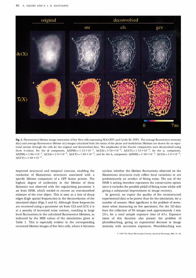
improved structural and temporal contrast, enabling theresolution of filamentous structures associated with aspecific lifetime component of a GFP fusion protein. Thehighest degree of uniformity in the lifetime of thesefilaments was observed with the regularising parameter l

set from ISNR, which tended to recover an oversmoothedestimate of the true object. This is seen as a loss of sharpedges (high spatial frequencies) in the deconvolution of thesimulated object (Figs 3 and 4). Although these frequenciesare recovered using a parameter set from CLS and GCV, it isat a penalty of increased noise content, resulting in largelocal fluctuations in the calculated fluorescence lifetimes, asindicated by the MSE values of the simulations given inTable 1. This is especially evident in the correspondingrecovered lifetime images of live Vero cells, where it becomes

unclear whether the lifetime fluctuations observed on thefilamentous structures truly reflect local variations or arepredominantly an artefact of fitting noise. The use of theISNR l setting therefore represents the conservative optionsince it excludes the possible pitfall of fitting noise whilst stillgiving a substantial improvement in image recovery.

In general, we expect the quality of the reconstructedexperimental data to be poorer than for the simulation, for anumber of reasons. Most significant is the problem of move-ment when measuring on live specimens. For the 3D datahere the collection of 96 images took approximately 1 min20 s, for a total sample exposure time of 43 s. Exposuretimes of this duration also present the problem ofphotobleaching, giving an exponential decrease in imageintensity with successive exposures. Photobleaching was

Fig. 5. Fluorescence lifetime image restoration of live Vero cells expressing NLS-GFP5 and Cyclin B1-YFP5. The average fluorescence intensitydc(x) and average fluorescence lifetime t(x) images calculated from the mean of the phase and modulation lifetimes are shown for an equa-torial section through the cells for the original and deconvolved data. The amplitudes of the Fourier components were deconvolved usingthree l-values. For the dc component, l(ISNR) ¼ 1·23 × 10¹2, l(CLS) ¼ 3·50 × 10¹6, l(GCV) ¼ 1·53 × 10¹6, for the a1 component,l(ISNR) ¼ 2·86 × 10¹2, l(CLS) ¼ 2·0 × 10¹6, l(GCV) ¼ 1·60 × 10¹6, and for the b1 component: l(ISNR) ¼ 2·38 × 10¹2, l(CLS) ¼ 2·0 × 10¹6,l(GCV) ¼ 1·60 × 10¹6.



compensated for in the measured PSF but not in the live celldata.

Much has been reported on the effects of sphericalaberration arising from the refractive index mismatchbetween the objective oil, coverslip and cell/medium onthe quality of reconstructed data (Hell & Stelzer, 1995). Amanifestation of this phenomenon is a lack of cylindricalsymmetry in measurements of the PSF. This is evident onlyto a slight degree in the PSF measurement used in thiswork, as seen in Fig. 6. For this reason we believe this effectplayed a relatively minor role in the quality of the recovereddata as compared with the effects discussed above. It wasfound to be of vital importance to the effectiveness of thereconstructions however, that the PSF be sampled over itsfull length. This occurs since the PSF of a wide-fieldmicroscope is found to be extensive in the z-dimension(Shaw & Rawlins, 1991), giving rise to elongated blur inthat direction. Furthermore, for full 3D reconstruction,sampling to a similar extent beyond the z-dimension of theobject is necessary. The presented methodology is alsoapplicable to confocal FLIM (So et al., 1995), where thefinite size of the PSF in the z-dimension should give animprovement over lifetime image restoration with the wide-field microscope. Despite this fact, the wide-field 3D FLIMshould gain through higher photon collection efficiency anddata acquisition speed.

We propose the use of simultaneous fluorescence lifetimediscrimination of different mutants of GFP-fusion proteinstargeted to distinct cellular compartments as an alternativeto spectral filtering. In the example given here, this involvedthe resolution of structures with distinct lifetimes over-lapping in three dimensions. For problems of this nature

the application of image deconvolution for unscramblinglifetime structures becomes critical.

Acknowledgements

We thank Dr Peter Verveer and Dr Thomas Jovin at thedepartment of Molecular Biology, Max Planck Institute forBiophysical Chemistry in Gottingen, Germany, for providingthe ICTM deconvolution algorithm, Dr Stephan Geley at theCell Cycle Control Laboratory, ICRF, for providing theplasmids of the GFP5 and YFP5 constructs, and Dr RainerPepperkok at the Light Microscopy Laboratory, ICRF, for themicroinjections performed on the Vero cells and criticallyreading the manuscript.

References

Aikens, R., Agard, D.A. & Sedat, J.W. (1989) Solid-state imagers formicroscopy. Methods Cell Biol. 29, 291–313.

Bastiaens, P.I.H. & Jovin, T.M. (1996) Microspectroscopic imagingtracks the intracellular processing of a signal transductionprotein: fluorescent-labeled protein kinase C bI. Proc. Natl. Acad.Sci. USA, 93, 8407–8412.

Bertero, M. & DeMol, C. (1996) Super-resolution by data inversion.Prog. Opt. 36, 129–178.

Buist, A.H., Muller, M., Gijsbers, E.J., Brakenhoff, G.J., Sosnowski,T.S., Norris, T.B. & Squier, J. (1997) Double-pulse fluorescencelifetime measurements. J. Microsc. 186, 212–220.

Carlsson, K. & Liljeborg, A. (1997) Confocal fluorescence micro-scopy using spectral and lifetime information to simultaneouslyrecord four fluorophores with high channel separation.J. Microsc. 185, 37–46.

Carrington, W.A., Lynch, R.M., Moore, E.D.W., Isenberg, G.,


Fig. 6. Point spread function measured in the FLIM apparatus: (A) xz section (B) xy section. Scale bars represent 1 mm and the vertical colourbar shows relative intensity, with red being the highest intensity.

3D-FLIM 47

Fogarty, K.E. & Fay, F.S. (1995) Superresolution three-dimensional images of fluorescence in cells with minimal lightexposure. Science, 268, 1483–1487.

Clegg, R.M., Feddersen, B.A., Gratton, E. & Jovin, T.M. (1992)Time-resolved imaging fluorescence microscopy. Proc. SPIE,1640, 448–460.

Clegg, R.M. & Schneider, P.C. (1996) Fluorescence lifetime-resolvedimaging microscopy: a general description of lifetime-resolvedimaging measurements. Fluorescence Microscopy and FluorescenceProbes (ed. by J. Slavik), pp. 15–33. Plenum Press, New York.

Dingwall, C., Robbins, J., Dilworth, S.M., Roberts, B. & Richardson,W.D. (1988) The nucleoplasmin nuclear location sequence islarger and more complex than that of SV-40 large T antigen.J. Cell Biol. 107, 841–849.

Dong, C.Y., So, P.T.C., French, T. & Gratton, E. (1995) Fluorescencelifetime imaging by asynchronous pump-probe microscopy.Biophys. J. 69, 2234–2242.

Gadella, T.W.J., Clegg, R.M. & Jovin, T.M. (1994) Fluorescencelifetime imaging microscopy: pixel-by-pixel analysis of phase-modulation data. Bioimaging, 2, 139–159.

Gadella, T.W.J. & Jovin, T.M. (1995) Oligomerization of epidermalgrowth-factor receptors on A431 cells studied by time-resolvedfluorescence imaging microscopy – a stereochemicalmodel for tyrosine kinase receptor activation. J. Cell Biol. 129,1543–1558.

Gadella, T.W.J., Jovin, T.M. & Clegg, R.M. (1993) Fluorescencelifetime imaging microscopy (FLIM) – spatial-resolution ofmicrostructures on the nanosecond time-scale. Biophys. Chem.48, 221–239.

Galatsanos, N.P. & Katsaggelos, A.K. (1992) Methods for choosingthe regularisation parameter and estimating the noise variancein image restoration and their relation. IEEE Trans. ImageProcess. 1, 322–336.

Gratton, E. & Limkeman, M. (1983) A continuously variablefrequency cross-correlation phase fluorometer with picosecondresolution. Biophys. J. 44, 315–324.

Hamamatsu-Photonics-K.K. (1995) Hamamatsu datasheet; C5825modulatable image intensifier.

Hell, S.W. & Stelzer, E.H.K. (1995) Lens aberrations in confocalfluorescence microscopy. Handbook of Biological Confocal Micro-scopy (ed. by J. B. Pawley), pp. 347–362. Plenum Press, NewYork.

Jackman, M., Firth, M. & Pines, J. (1995) Human cyclins B1 andB2 are localized to strikingly different structures: B1 tomicrotubules, B2 primarily to the Golgi apparatus. EMBO J.14, 1646–1654.

Jutamulia, S., Asakura, T. & Ambar, H. (1985) Reduction ofcoherent noise using various artificial incoherent sources. Optik,70, 52–57.

Katsaggelos, A.K., Biemond, J., Schafer, R.W. & Mersereau, R.M.(1991) A regularized iterative image-restoration algorithm. IEEETrans. Signal Process. 39, 914–929.

Katsaggelos, A.K. & Efstratiadis, S.N. (1990) A class of iterativesignal restoration algorithms. IEEE Trans. Acoust. Speech SignalProcess. 38, 778–786.

Katsaggelos, A.K. & Lay, K.T. (1991) Maximum-likelihood bluridentification and image-restoration using the EM algorithm.IEEE Trans. Signal Process. 39, 729–733.

van Kempen, G.M.P., van Vliet, L.J., Verveer, P.J. & van derVoort, H.T.M. (1997) A quantitative comparison of imagerestoration methods for confocal microscopy. J. Microsc. 185,354–365.

Krishnamurthi, V., Liu, Y.H., Bhattacharyya, S., Turner, J.N. &Holmes, T.J. (1995) Blind deconvolution of fluorescencemicrographs by maximum-likelihood-estimation. Appl. Opt. 34,6633–6647.

Kume, H., Koyama, K., Nakatsugawa, K., Suzuki, S. & Fatlowitz, D.(1988) Ultrafast microchannel plate photomultipliers. Appl. Opt.27, 1170–1178.

Lakowicz, J.R. & Berndt, K. (1991) Lifetime-selective fluorescenceimaging using an rf phase-sensitive camera. Rev. Sci. Instrum.62, 1727–1734.

Lakowicz, J.R. & Maliwal, B.P. (1985) Construction and perfor-mance of a variable-frequency phase-modulation fluorometer.Biophys. Chem. 21, 61–78.

Lakowicz, J.R., Szmacinski, H., Lederer, W.J., Kirby, M.S.,Johnson, M.L. & Nowaczyk, K. (1994) Fluorescence lifetimeimaging of intracellular calcium in COS cells using Quin-2. CellCalcium, 15, 7–27.

Mizushima, S. & Nagata, S. (1990) pEF-BOS: a powerfulmammalian expression vector. Nucl. Acid Res. 18, 5322.

Morgan, C.G., Murray, J.G. & Mitchell, A.C. (1995) Photon-correlation system for fluorescence lifetime measurements. Rev.Sci. Instrum. 66, 3744–3749.

Piston, D.W., Marriott, G., Radivoyevich, T., Clegg, R.M., Jovin, T.M.& Gratton, E. (1989) Wideband acoustooptic light-modulator forfrequency-domain fluorometry and phosphorimetry. Rev. Sci.Instrum. 60, 2596–2600.

Press, W.H., Flannery, B.P., Teukolky, S.A. & Vetterling, W.T. (1990)Numerical Recipes in C – The Art of Scientific Computing, pp. 735.Cambridge University Press, Cambridge.

Sanders, R., Draaijer, A., Gerritsen, H.C., Houpt, P.M. & Levine, Y.K.(1995) Quantitative pH imaging in cells using confocalfluorescence lifetime imaging microscopy. Anal. Biochem.. 227,302–308.

Schneider, P.C. & Clegg, R.M. (1997) Rapid acquisition, analysis,and display of fluorescence lifetime-resolved images for real-timeapplications. Rev. Sci. Instrum. 68, 4107–4119.

Shaw, P. (1994) Deconvolution in 3-D optical microscopy.Histochem. J. 26, 687–694.

Shaw, P.J. & Rawlins, D.J. (1991) The point-spread function of aconfocal microscope: its measurement and use in deconvolutionof 3-D data. J. Microsc. 163, 151–165.

So, P.T.C., French, T., Yu, W.N., Berland, K., Dong, C.Y. & Gratton,E. (1995) Time-resolved fluorescence microscopy using two-photon excitation. Bioimaging, 3, 1–15.

Spencer, R.D. & Weber, G. (1969) Measurements of subnanosecondfluorescence lifetime with a cross-correlation phase fluorometer.Ann. NY Acad. Sci. 158, 361–376.

Szmancinski, H. & Lakowicz, J.R. (1995) Possibility ofsimultaneously measuring low and high-calcium concentrationsusing Fura-2 and lifetime-based sensing. Cell Calcium, 18, 64–75.

Tikhonov, A.N. & Arsenin, V.Y. (1977) Solutions of Ill-PosedProblems. Wiley, New York.

Van der Voort, H.T.M. & Brakenhoff, G.J. (1990) 3-D image



formation in high-aperture fluorescence confocal microscopy: anumerical analysis. J. Microsc. 158, 43–54.

Van der Voort, H.T.M. & Strasters, K.C. (1995) Restoration ofconfocal images for quantitative image-analysis. J. Microsc. 178,165–181.

Verveer, P.J. & Jovin, T.M. (1997) Efficient superresolutionrestoration algorithms using maximum a posteriori estimationswith application to fluorescence microscopy. J. Opt. Soc. Am. A,14, 1696–1706.

Vitria, J. & Llacer, J. (1996) Reconstructing 3D light microscopicimages using the EM algorithm. Pattern Recognition Lett. 17,1491–1498.

Zernicka-Goetz, M., Pines, J., McLean Hunter, S., Dixon, J.P.,Siemering, K.R., Haseloff, J. & Evans, M.J. (1997) Followingcell fate in the living mouse embryo. Development, 124,1133–1137.


3D-FLIM 49

Three dimensional image restoration in ﬂuorescence ... · Three dimensional image restoration in...

Documents

Transcript of Three dimensional image restoration in ﬂuorescence ... · Three dimensional image restoration in...