Three-Dimensional Green’s Function and Its Derivatives for ...

Three-Dimensional Green’s Function

and Its Derivatives for Anisotropic

Elastic, Piezoelectric and

Magnetoelectroelastic Materials

THESIS

in fulfillment of the requirements for the degree ofDoctor of Engineering (Dr.-Ing.)

at the Faculty of Science and Technologyof the University of Siegen

byLongtao Xie

First reviewer (Advisor): Prof. Dr.-Ing. habil. Dr. h.c. Chuanzeng ZhangSecond reviewer: Prof. Dr.-Ing. habil. Wilfried Becker

Date of the oral examination: July 15, 2016

Siegen, August 2016

AbstractThis thesis mainly deals with the Green’s function for linear generally anisotropic mate-rials in the infinite three-dimensional space, also called the fundamental solution. Thedetailed derivations and the numerical results of the explicit expressions of the Green’sfunction and its first and second derivatives based on the residue calculus method (RCM),Stroh formalism method (SFM) and unified explicit expression method (UEEM) are pre-sented. The numerical examples of the three different methods are compared with eachother for the anisotropic elasticity. All three methods are accurate for an arbitrary pointin non-degenerate cases. For nearly degenerate cases, both the RCM and the SFM becomeunstable while the UEEM keeps accurate. Moreover, the SFM is more stable than theRCM. To overcome the difficulty in nearly degenerate cases and degenerate cases, somematerial constants are slightly changed in the RCM and the SFM. Although the UEEMhas some advantages compared with the RCM and the SFM, it is difficult to be extendedto the multifield coupled materials. The RCM and SFM are extended to the piezoelectricmaterials and compared with each other. Since the SFM has a better performance thanthe RCM for the piezoelectric materials, it is extended further to the magnetoelectroelas-tic materials. The UEEM is implemented into a Boundary Element Method (BEM) as anapplication. Some demonstrative anisotropic elastic problems are solved by the developedBEM.

ZusammenfassungDiese Arbeit behandelt hauptsachlich die Greensche Funktion fur lineare allgemein anisotropeMaterialien im unendlichen dreidimensionalen Raum, die auch als Fundamentallosungbezeichnet wird. Die detaillierten Herleitungen und die numerischen Auswertungen derexpliziten Ausdrucke der Greenschen Funktion bzw. deren ersten und zweiten Ableitung,die auf der Methode der Residuen (RCM), dem Stroh-Formalismus (SFM) sowie derUnified Explicit Expression Method (UEEM) basieren, werden ebenfalls behandelt. Dienumerischen Beispiele der drei verschiedenen Methoden werden fur die Elastizitatstheoriemiteinander verglichen. In nicht-degenerierten Fallen sind alle drei Methoden exakt fureinen beliebigen Punkt. Bei nahezu degenerierten Fallen werden sowohl die RCM alsauch die SFM instabil, wahrend die UEEM ihre Gultigkeit behalt. Ungeachtet dessen istdie SFM etwas stabiler als die RCM. Um deren Instabilitat in degenerierten und nahezudegenerierten Fallen zu uberwinden, werden in der RCM und der SFM einige Materialkon-stanten leicht modifiziert. Trotz der Vorteile der UEEM im Vergleich zu RCM und SFM,ergeben sich Schwierigkeiten bei der Erweiterung auf Mehrfeldmaterialien. Die RCM unddie SFM werden auf piezoelektrische Materialien erweitert und miteinander verglichen.Dadurch, dass die SFM bessere Ergebnisse fur piezoelektrische Materialien liefert als die

RCM, wird sie zusatzlich auf magnetoelektroelastische Materialien erweitert. Daruberhinaus wird die UEEM als Anwendung in einem BEM-Programm implementiert, mitdem sich einfache Elastizitatsprobleme losen lassen.

Acknowledgments

This thesis was completed in the course of my research activity as a PhD candidate from2011 to 2016 at the Chair of Structural Mechanics, Department of Civil Engineering,University of Siegen, Germany.

I would like to thank my advisor, Prof. Dr.-Ing. habil. Dr. h.c. Chuanzeng Zhang asthe first reviewer of my thesis, for his supervision. His scientific vision has always inspiredand motivated my research work. I am very grateful to him for his patience, immenseand continuous support. His guidance helped me in the whole PhD study including thewriting of this thesis. This thesis could not have been completed without his help andsupport.

My sincere thanks to Prof. Dr.-Ing. habil. Wilfried Becker as the second reviewerof my thesis for his precious time spent to read and check my thesis in details, and hisvaluable comments and suggestions to improve the thesis. I would like also to thankProf. Dr.-Ing. Torsten Leutbecher and Prof. Dr.-Ing. Ulrich Schmitz as members of theDoctoral Commission for their time and effort.

I would like to thank Professor Chyanbin Hwu from the National Cheng Kung Uni-versity, Taiwan. During his scientific visit at the Chair of Structural Mechanics of theUniversity of Siegen we had a lot of scientific discussions especially on the powerful Strohformalism method, which have been very helpful for my PhD work. My sincere thanksalso to Professor Ernian Pan from the University of Akron, USA, for valuable discussionsin the course of my PhD study.

I would like to thank my colleagues Meike Stricker, Pedro Villamil, Hui Zheng, Ben-jamin Ankay, Elias Perras and many our former and current international guests at theChair of Structural Mechanics for giving me a pleasant working atmosphere.

Finally, I would like to thank my family, particularly my parents and my wife, for thecontinuous support, encouragement, patience and love that I have received.

This work is supported by the China Scholarship Council (CSC), which is also grate-fully acknowledged.

August 2016, Siegen Longtao Xie

Contents

Contents i

List of Figures v

List of Tables vii

1 Introduction 11.1 Anisotropic materials and Green’s function . . . . . . . . . . . . . . . . . . 11.2 State of the art and objectives . . . . . . . . . . . . . . . . . . . . . . . . . 21.3 Overview of the thesis . . . . . . . . . . . . . . . . . . . . . . . . . . . . . 4

2 Mathematical preliminaries 52.1 Basic equations of anisotropic linear elasticity . . . . . . . . . . . . . . . . 52.2 Basic equations of linear piezoelectricity . . . . . . . . . . . . . . . . . . . 62.3 Basic equations of linear magnetoelectroelasticity . . . . . . . . . . . . . . 72.4 Stroh formalism . . . . . . . . . . . . . . . . . . . . . . . . . . . . . . . . . 9

2.4.1 A general solution in anisotropic linear elasticity . . . . . . . . . . . 92.4.2 Stroh eigenvalue problem for an oblique plane . . . . . . . . . . . . 10

2.5 Fundamentals of the Green’s function . . . . . . . . . . . . . . . . . . . . . 112.5.1 Green’s function in boundary value problems . . . . . . . . . . . . . 112.5.2 Green’s function for multifield coupled media . . . . . . . . . . . . 12

2.6 Boundary integral equations . . . . . . . . . . . . . . . . . . . . . . . . . . 12

3 Green’s function in anisotropic linear elasticity 153.1 Problem statement . . . . . . . . . . . . . . . . . . . . . . . . . . . . . . . 153.2 Line integral Green’s function and its derivatives . . . . . . . . . . . . . . . 163.3 Explicit Green’s function and its derivatives . . . . . . . . . . . . . . . . . 19

3.3.1 Residue calculus method . . . . . . . . . . . . . . . . . . . . . . . . 193.3.2 Stroh formalism method . . . . . . . . . . . . . . . . . . . . . . . . 21

3.4 Unified explicit Green’s function and its derivatives . . . . . . . . . . . . . 243.4.1 Rearrangements of the integrals . . . . . . . . . . . . . . . . . . . . 243.4.2 Unified explicit expressions . . . . . . . . . . . . . . . . . . . . . . . 27

3.5 Verifications and comparison of the different methods . . . . . . . . . . . . 303.5.1 Verification of the numerical integration method . . . . . . . . . . . 323.5.2 Verification of the residue calculus method . . . . . . . . . . . . . . 343.5.3 Verification of the Stroh formalism method . . . . . . . . . . . . . . 353.5.4 Verification of the unified explicit expressions . . . . . . . . . . . . 363.5.5 Comparison of the efficiency . . . . . . . . . . . . . . . . . . . . . . 37

i

3.6 Numerical examples . . . . . . . . . . . . . . . . . . . . . . . . . . . . . . . 383.6.1 Numerical results near the degenerated point . . . . . . . . . . . . . 383.6.2 Numerical results for an arbitrary point on a unit sphere . . . . . . 42

3.7 Concluding remarks . . . . . . . . . . . . . . . . . . . . . . . . . . . . . . . 42

4 Green’s function in linear piezoelectricity 454.1 Problem statement . . . . . . . . . . . . . . . . . . . . . . . . . . . . . . . 454.2 Stroh formalism method . . . . . . . . . . . . . . . . . . . . . . . . . . . . 46

4.2.1 Representation of the Green’s function . . . . . . . . . . . . . . . . 464.2.2 First derivative of the Green’s function . . . . . . . . . . . . . . . . 474.2.3 Second derivative of the Green’s function . . . . . . . . . . . . . . . 48

4.3 Residue calculus method . . . . . . . . . . . . . . . . . . . . . . . . . . . . 494.3.1 Representation of the Green’s function . . . . . . . . . . . . . . . . 494.3.2 First derivative of the Green’s function . . . . . . . . . . . . . . . . 504.3.3 Second derivative of the Green’s function . . . . . . . . . . . . . . . 51

4.4 Numerical procedures . . . . . . . . . . . . . . . . . . . . . . . . . . . . . . 524.5 Numerical examples and discussions . . . . . . . . . . . . . . . . . . . . . . 534.6 Concluding remarks . . . . . . . . . . . . . . . . . . . . . . . . . . . . . . . 60

5 Green’s function in linear magnetoelectroelasticity 615.1 Problem statement . . . . . . . . . . . . . . . . . . . . . . . . . . . . . . . 615.2 Stroh formalism method . . . . . . . . . . . . . . . . . . . . . . . . . . . . 62

5.2.1 Representation of the Green’s function . . . . . . . . . . . . . . . . 635.2.2 First derivative of the Green’s function . . . . . . . . . . . . . . . . 645.2.3 Second derivative of the Green’s function . . . . . . . . . . . . . . . 65

5.3 Numerical examples and discussions . . . . . . . . . . . . . . . . . . . . . . 655.4 Concluding remarks . . . . . . . . . . . . . . . . . . . . . . . . . . . . . . . 67

6 Applications of the Green’s function and its derivatives in the BEM 816.1 Preliminary remarks . . . . . . . . . . . . . . . . . . . . . . . . . . . . . . 816.2 Description of the BEM for anisotropic linear elasticity . . . . . . . . . . . 826.3 Numerical examples . . . . . . . . . . . . . . . . . . . . . . . . . . . . . . . 83

6.3.1 Cube under tension . . . . . . . . . . . . . . . . . . . . . . . . . . . 836.3.2 Cube with a spheroidal cavity under tension . . . . . . . . . . . . . 85

6.4 Concluding remarks . . . . . . . . . . . . . . . . . . . . . . . . . . . . . . . 87

7 Summary and outlook 91

A Residue calculus of an improper line integral 93

B Explicit expressions of N,i and N,ij 95

C Auxiliary functions F (n)m for the second derivative of the Green’s function 97

D Explicit expression of the Stroh eigenvector ξ 101

ii

Bibliography 103

iii

List of Figures

3.1 An illustration on the unit sphere S2, the oblique plane perpendicular tox, the unit circle S1, ξ in S1, n, m and ψ. . . . . . . . . . . . . . . . . . . 18

3.2 Diagram of the Stroh formalism method. . . . . . . . . . . . . . . . . . . . 313.3 Diagram of the unified explicit expression method with known Stroh eigen-

values. . . . . . . . . . . . . . . . . . . . . . . . . . . . . . . . . . . . . . . 323.4 The maximum relative errors in Gij, Gij,1 and Gij,11 versus the number of

Gaussian points for the transversely isotropic materials Mg and C at point(1, 2, 3). . . . . . . . . . . . . . . . . . . . . . . . . . . . . . . . . . . . . . 34

3.5 The CPU time for calculating the Green’s function and its derivatives bythe four methods. . . . . . . . . . . . . . . . . . . . . . . . . . . . . . . . . 38

3.6 Numerical evaluations of the Green’s function around the denegerated pointfor the transversely isotropic material Mg . . . . . . . . . . . . . . . . . . . 40

3.7 Numerical evaluations of the first derivatvie of the Green’s function aroundthe denegerated point for the transversely isotropic material Mg . . . . . . 40

3.8 Numerical evaluations of the second derivatvie of the Green’s functionaround the denegerated point for the transversely isotropic material Mg . . 41

3.9 Spherical coordinates of the field point x . . . . . . . . . . . . . . . . . . . 423.10 General evaluation of the anisotropic elastic Green’s function by the UEEM. 433.11 General evaluation of the first derivative of the anisotropic elastic Green’s

function by the UEEM. . . . . . . . . . . . . . . . . . . . . . . . . . . . . . 433.12 General evaluation of the second derivative of the anisotropic elastic Green’s

function by the UEEM. . . . . . . . . . . . . . . . . . . . . . . . . . . . . . 44

4.1 Diagonal components of the Green’s function for PZT at field points . . . . 564.2 Non-diagonal components of the Green’s function for PZT at field points . 574.3 Some components of the first derivative of the Green’s function for PZT at

field points . . . . . . . . . . . . . . . . . . . . . . . . . . . . . . . . . . . . 584.4 Some components of the second derivative of the Green’s function for PZT

at field points . . . . . . . . . . . . . . . . . . . . . . . . . . . . . . . . . . 59

5.1 Variation of the Green’s function GIJ on upper half unit sphere with thesource point at the origin. . . . . . . . . . . . . . . . . . . . . . . . . . . . 69

5.2 Variation of the first derivative of the Green’s function GIJ,1 on upper halfunit sphere with the source point at the origin. . . . . . . . . . . . . . . . . 70


v


5.5 Variation of the second derivative of the Green’s function GIJ,11 on upperhalf unit sphere with the source point at the origin. . . . . . . . . . . . . . 73






6.1 Transformation of a boundary element to a local reference element . . . . . 826.2 One-eighth of a cube under tension . . . . . . . . . . . . . . . . . . . . . . 846.3 Rotations of the coordinates. . . . . . . . . . . . . . . . . . . . . . . . . . . 856.4 Model of the cube with a cavity under tension. . . . . . . . . . . . . . . . . 866.5 The mesh of the cube with a spheroidal cavity . . . . . . . . . . . . . . . . 876.6 The displacement u1 on the edges of the one-eighth spheroid. . . . . . . . . 876.7 The displacement u2 on the edges of the one-eighth spheroid. . . . . . . . . 886.8 The displacement u3 on the edges of the one-eighth spheroid. . . . . . . . . 88

A.1 The contour Γ. . . . . . . . . . . . . . . . . . . . . . . . . . . . . . . . . . 94

vi

List of Tables

3.1 Components of the Green’s function and its derivatives by the numericalintegration method with 25 Gaussian points and analytical solutions fortransversely isotropic material Mg at the point (1, 2, 3). . . . . . . . . . . . 33

3.2 Components of the Green’s function and its derivatives by the numericalintegration method with 25 Gaussian points and analytical solutions fortransversely isotropic material C at the point (1, 2, 3). . . . . . . . . . . . . 33

3.3 Components of the Green’s function and its derivatives by the residue cal-culus method for transversely isotropic materials Mg and C at the point(1, 2, 3). . . . . . . . . . . . . . . . . . . . . . . . . . . . . . . . . . . . . . 35

3.4 Components of the Green’s function and its derivatives by the Stroh for-malism method for transversely isotropic materials Mg and C at the point(1, 2, 3). . . . . . . . . . . . . . . . . . . . . . . . . . . . . . . . . . . . . . 36

3.5 Components of the Green’s function and its derivatives by the unified ex-plicit expression method for transversely isotropic materials Mg and C atthe point (1, 2, 3). . . . . . . . . . . . . . . . . . . . . . . . . . . . . . . . . 37

4.1 Components of the Green’s function GIJ for PZT at point (1, 2, 3) . . . . . 544.2 Components of the first derivative of the Green’s function GIJ,1 for PZT

at point (1, 2, 3) . . . . . . . . . . . . . . . . . . . . . . . . . . . . . . . . . 554.3 Components of the second derivative of the Green’s function GIJ,11 for PZT

at point (1, 2, 3) . . . . . . . . . . . . . . . . . . . . . . . . . . . . . . . . . 554.4 Computing time for the Green’s function and its derivatives for PZT at

point (1, 2, 3) . . . . . . . . . . . . . . . . . . . . . . . . . . . . . . . . . . 55

5.1 Numerical results of the Green’s function Gij(×10−6) at the point (1, 2, 3)m. 665.2 Numerical results of the components of the first derivative of the Green’s

function Gij,k(×10−7) at the point (1, 2, 3)m. . . . . . . . . . . . . . . . . . 675.3 Numerical results of the components of the second derivative of the Green’s

function Gij,kl(×10−7) at the point (1, 2, 3)m. . . . . . . . . . . . . . . . . . 685.4 The CPU time for the calculation of the Green’s function and its derivatives

by the novel explicit expressions . . . . . . . . . . . . . . . . . . . . . . . . 68

6.1 Displacements of the cube under tension with transversely isotropic mate-rial Mg . . . . . . . . . . . . . . . . . . . . . . . . . . . . . . . . . . . . . . 84

6.2 Displacements of the cube under tension with rotated transversely isotropicmaterial Mg; ui are the present results; uci are evaluated by COMSOLMultiphysics with 1000 elements. . . . . . . . . . . . . . . . . . . . . . . . 86

vii

Chapter 1

Introduction

1.1 Anisotropic materials and Green’s functionA material is said to be anisotropic when the deformation behavior of the material dependsupon the orientation; that is, the stress-strain response of the material in one directionis different from the others. An anisotropic material is quite different from an isotropicmaterial whose properties keep the same along all directions. Although the isotropicmaterial is easy to understand since most theories of elasticity are valid for isotropicmaterials, the anisotropic materials are more common in the nature and daily life.

Early investigations of the anisotropy were motivated by the response of the natu-rally anisotropic materials such as wood and crystalline solids. Anisotropic materials mayhave special symmetries. Metals are typical anisotropic crystalline solids. They can bedivided into many classes according to their symmetry properties. Among the commonlyused metals, Al, Cu, Ni and Ag are cubic materials, Mg, Zn and Al2O3 are hexagonal ortransversely isotropic materials, and Sn and Zr are tetragonal materials. In the moderntechnology, the extensive use of the composites (Jones, 1998) has brought forward manynew types of anisotropic materials. Recently, the magnetoelectroelastic coupling com-posite materials have attracted much attention from engineers and scientists due to themulti-physical energy conversion capacities and the design ability. Most composites areessentially anisotropic.

A proper modeling of the behaviors of the anisotropic materials is required by thedesigns and applications of the anisotropic materials. In the linear theory of elasticity,the anisotropic property of materials is described by a symmetric matrix establishing arelation between the stresses and the strains. For a certain type of anisotropic materialsreferred to a coordinate system based on the symmetry of the materials, the matrix canbe of a simple form, i.e., most components of the matrix are zero and the number of theindependent non-zero components of the matrix is small. For example, a transverselyisotropic elastic material referred to a Cartesian coordinate system with the x3-axis alongthe symmetry axis of the material has 12 non-zero components, among which only 5components are independent. For a generally anisotropic material, the symmetric matrixhas 21 independent components which increases the difficulty to obtain the solution ofa particular problem for the anisotropic materials. Although with a proper choice onthe coordinate system the matrix of many materials can be kept simple, any transfor-mation of the coordinate system will cause the matrix to be mathematically generallyanisotropic. Therefore general theory for the generally anisotropic materials is preferred.

1

The theoretical formulations presented in this thesis are for generally or fully anisotropicmaterials.

The Green’s function is a powerful tool to solve the boundary value problems. It can beused to solve many anisotropic problems in the applied mechanics and solid physics suchas dislocation problems, inhomogeneous problems and contact problems. The derivativesof the Green’s function are usually required to obtain the internal stresses in the solids.Moreover, the Green’s function and its derivatives are the basic stones of the bound-ary integral equation method or the boundary element method (BEM), which severalhas advantages in the numerical analysis of many engineering problems such as fracturemechanics problems and acoustic problems especially in the infinite domain.

Physically speaking, the Green’s function is the response at an observation point dueto a point source applied at a particular point. When the domain is infinite, the Green’sfunction is also referred to as the displacement fundamental solution of the problem.The static Green’s function in the infinite domain is simply called the Green’s functionthroughout this thesis unless special statement is given. In elasticity, the Green’s functionfor the isotropic materials has a simple form, while it is complicated for the generallyanisotropic materials. The analytical or exact Green’s function is only available for specialcases of anisotropic materials such as the transversely isotropic materials (Dederichs andLiebfried, 1969; Pan and Chou, 1976). The study on the anisotropic Green’s functioncan be traced back to the works of Fredholm (1900), Lifshitz and Rozenzweig (1947) andSynge (1957). In the early research of the Green’s function, many approximate solutions ofthe Green’s function were presented (Barnett, 1972; Gundersen and Lothe, 1987; Lie andKoehler, 1968; Mura, 1987). Recently, Shiah et al. (2012) presented an efficient evaluationof the Green’s function and its derivatives by representing the Green’s function as a Fourierseries and Tan et al. (2013) applied the evaluation technique in the BEM. Wang (1997)re-investigated the explicit expression of the Green’s function for generally anisotropicmaterials and suggested a mall perturbation on the material constants for the practicalapplications. Since then many efforts have been made to derive the explicit expressions ofthe Green’s function and its derivatives. The works of Malen (1971), Lavagnino (1995),Ting and Lee (1997), Sales and Gray (1998), Lee (2003) and Buroni and Saez (2013)should be cited here among others. Here the word explicit means that no numericalintegration or differentiation method is needed in the calculation.

The main topic of this thesis is the derivation of the explicit expressions of the Green’sfunction and its first and second derivatives for the three-dimensional (3D) generallyanisotropic materials including linear elastic, piezoelectric and magnetoelectroelastic ma-terials. Although the Green’s function for 3D anisotropic elastic materials has been in-vestigated very comprehensively since many years, it is still a highly demanding issueespecially in the BEM community where an accurate and efficient numerical evaluationof the Green’s function and its derivatives is especially important.

1.2 State of the art and objectivesThe line integral expression of the Green’s function was first presented by Fredholm (1900).There are mainly two ways to evaluate the Green’s function explicitly. A straightforwardway is to apply the residue calculus to the line integral, which leads to an expression interms of the roots of a polynomial equation. The other way is using the so called Stroh

2

formalism method, in which the expression is constructed from the eigenvectors of theStroh eigenvalue problem (Malen, 1971). The relation between the two approaches is thatthe roots of the polynomial equation in the first approach is identical to the eigenvaluesof the Stroh eigenvalue problem in the second approach. The roots and the eigenvaluesare both called the Stroh eigenvalues. In these two approaches, the expression for distinctStroh eigenvalues is different from that for the repeated or degenerated Stroh eigenval-ues. For the general application, additional numerical treatments should be made, forexample by a small perturbation on the material constants. To overcome the degeneracyproblem with repeated Stroh eigenvalues, Ting and Lee (1997) proposed a unified explicitexpression of the Green’s function. Here the word unified means that after a rewritten ofthe expression for distinct Stroh eigenvalues, the expression remains applicable even whenthe Stroh eigenvalues are identical. The word unified is used to emphasize the differencefrom the explicit expression which changes when the multiplicity of the Stroh eigenvalueschanges.

Due to their applications in the BEM for the analysis of the anisotropic elastic bound-ary value problems, many efforts have been made to derive the explicit expressions forthe first and second derivatives of the Green’s function. Most existing expressions areobtained by taking the derivatives of the Green’s function with respect to the sphericalcoordinates, which can be transformed to the Cartesian coordinate system if necessary.Some representative examples of the previous investigations on the topic are the worksby Sales and Gray (1998), Lavagnino (1995), Phan et al. (2004, 2005), Lee (2009), Shiahet al. (2010) and Buroni and Saez (2013). The explicit expressions with high-order tensorsin the Cartesian coordinate system were presented by Lee (2003) and Buroni and Saez(2010). Different from the other works, Buroni and Saez (2013) suggested a way to findunified expressions which remain applicable even when the Stroh eigenvalues degenerateor become identical.

The main aim of this thesis is to derive and investigate several explicit expressionsof the Green’s function and its first and second derivatives for the generally anisotropiclinear elastic, piezoelectric and magnetoelectroelastic materials and their numerical eval-uations. With the explicit expressions given in the Cartesian coordinate system, the mainobjectives of this thesis are

• to present alternative explicit expressions of the derivatives of the Green’s functionby using the residue calculus method, the Stroh formalism method and the methodsimilar to that suggested by Ting and Lee (1997);

• to give a comparison of the three explicit expressions regarding their accuracy andefficiency in the numerical calculations for the anisotropic linear elastic materials;

• to obtain new explicit expressions for the linear piezoelectric and magnetoelectroe-lastic materials; and finally,

• to implement the unified explicit expressions into a BEM and conduct the verifica-tion tests by numerical examples.

3

1.3 Overview of the thesisThroughout this thesis a vector, a tensor or a matrix is given either in index notation orrepresented by a bold letter. The summation convention is applied over repeated indicesunless otherwise explicitly declared. The lowercase Latin indices take the values 1, 2, 3,while the capital Latin indices take the values 1, 2, 3, 4 for piezoelectric materials, and1, 2, 3, 4, 5 for magnetoelectroelastic materials. A comma after a quantity (),i denotesspatial derivatives.

After a brief introduction in this chapter, Chapter 2 presents some theoretical foun-dations which are essential to the study of the Green’s function for anisotropic materials.In particular, the basic equations for the anisotropic linear elastic, piezoelectric and mag-netoelectroelastic materials, the classical Stroh formalism and the basic concepts of theGreen’s function are introduced. In addition, the boundary integral equations for 3Dgenerally anisotropic and linear elastic materials are presented as an application of theGreen’s function and its derivatives.

In Chapter 3, three different explicit expressions of the Green’s function and its firstand second derivatives for the generally anisotropic linear elastic materials are presented.Besides, the numerical integration method to calculate the Green’s function and its deriva-tives are also presented. All the four methods are coded into FORTRAN programs andcompared with each other through numerical examples in details.

In Chapter 4, based on the comparison between the numerical evaluations of the dif-ferent expressions in Chapter 3, the explicit expressions by using the residue calculusmethod and the Stroh formalism method are extended to the anisotropic linear piezoelec-tric materials. The two methods are verified by the analytical solutions and comparedwith each other with respect to their efficiency and accuracy.

In Chapter 5, the explicit expressions of the Green’s function and its derivatives bythe Stroh formalism method are further extended to the anisotropic linear magnetoelec-troelastic materials, since they have advantages in the accuracy and efficiency comparedwith the expressions by the residue calculus method.

In Chapter 6, the unified explicit expressions for anisotropic linear elastic materialsare implemented into a BEM program, since they seem to be most accurate and efficient.The BEM program is tested by some examples.

The last chapter summarizes the thesis with some concluding remarks and an outlookon future research works.

4

Chapter 2

Mathematical preliminaries

This chapter is about some basic aspects related to the study of the Green’s functionfor the anisotropic materials in the three-dimensional infinite space. The basic equationsfor the elastic, piezoelectric and magnetoelectroelastic materials are introduced in Sec-otins 2.1, 2.2 and 2.3, respectively. In Section 2.4, the Stroh formalism, which is veryuseful in solving the problems with anisotropic materials, is presented briefly with anemphasis on the Stroh eigenvalue problem for an oblique plane, which will be used in thefollowing chapters. In Section 2.5, the role of the Green’s function in a general differ-ential equation and the basic knowledge of the Green’s function for multifield materialsare discussed. Finally, the application of the Green’s function and its derivatives in theboundary integral equations are shown in the last section.

2.1 Basic equations of anisotropic linear elasticityFor a 3D linear and homogeneous elastic solid, when it is distorted the strain tensor εijis related to the derivative of the displacement ui by

εij = (ui,j + uj,i)/2, (2.1)

where the comma (),i denotes the spatial derivative. The components of the strain tensorεij are to be distinguished from the usual engineering strains which are equal to εij fori = j, but twice the value for i 6= j.

The general linear relation between the stress σij and the strain εij is usually given byHooke’s law

σij = cijklεkl, (2.2)where the fourth-order tensor cijkl is the elastic stiffness tensor or the elasticity tensor. Itpossesses full symmetry

cijkl = cjikl = cijlk = cklij (2.3)and is positive definite in the sense that

cijklεijεkl > 0 (2.4)

for any non-zero strain tensor εij.Considering the body force fi, the static equilibrium equation is given by

σij,i + fj = 0, (2.5)

5

The governing equation in terms of the displacement ui for the elasticity problems canbe obtained by substituting the Eqs. (2.1) and (2.2) into Eq. (2.5), i.e.,

cijkluk,li + fj = 0. (2.6)

2.2 Basic equations of linear piezoelectricityWe consider a linear and homogeneous piezoelectric solid in a 3D Cartesian coordinatesystem. The static equilibrium equation and the electrostatic equation are given by

σij,i + fj = 0,Di,i − f e = 0,

(2.7)

where Di and f e are the electric displacement vector and the electric charge density,respectively. The relation between the electric field Ei and the electric potential φ isdefined by the equation

Ei = −φ,i. (2.8)

The linear constitutive relations between σij, Di, εij and Ei are

σij = cijmnεmn − enijEn,Di = eimnεmn + κinEn,

(2.9)

where eimn and κin are the piezoelectricity tensor and the dielectricity tensor, respectively.They have the following symmetry relations

eimn = einm, κin = κni. (2.10)

Moreover the dielectricity tensor κij is positive definite, i.e.,

κijEiEj > 0, (2.11)

for any non-zero electric field vector Ei.The basic equations (2.7)-(2.9) can be written into a compact form by introducing the

generalized stress and strain tensors and the generalized displacement vector as (Barnettand Lothe, 1975)

σiJ =

σij, J = j ≤ 3,Di, J = 4,

(2.12a)

εMn =

εmn, M = m ≤ 3,−En, M = 4,

(2.12b)

uI =

ui, I = i ≤ 3,φ, I = 4.

(2.12c)

With Eq. (2.12), Eq. (2.7) becomes

σiJ,i + fJ = 0, (2.13)

6

where

fJ =

fj, J = j ≤ 3,−f e, J = 4,

(2.14)

and Eq. (2.9) becomesσiJ = ciJMnεMn = ciJMnuM,n, (2.15)

where

ciJMn =

cijmn, J = j ≤ 3, M = m ≤ 3,enij, J = j ≤ 3, M = 4,eimn, J = 4, M = m ≤ 3,−κin, J = 4, M = 4,

(2.16)

with the symmetry relationciJMn = cnMJi. (2.17)

Substituting Eq. (2.15) into Eq. (2.13), we have the governing equations in terms ofthe generalized displacement

ciJMnuM,ni + fJ = 0. (2.18)

2.3 Basic equations of linear magnetoelectroelastic-ity

Let us consider a magnetoelectroelastic solid in a fixed 3D Cartesian coordinate systemxi (i = 1, 2, 3). The equilibrium equations and the Gauss equations are given by

σij,i + fj = 0,Di,i − f e = 0, (2.19)Bi,i − fm = 0,

where Bi and fm are the magnetic induction vector and the magnetic charge density,respectively.

It should be remarked here that according to Maxwell’s equations for magnetism, themagnetic charge density fm is always zero, because there are no magnetic monopolesobserved (Fitzpatrick, 2008). However, the magnetic charge density fm is taken intoaccount in this study as in many other references in literature, just for the mathematicalconvenience.

The gradient equation representing magnetic field-potential relation is determined by

Hi = −ψ,i, (2.20)

where Hi and ψ are the magnetic field vector and the magnetic potential, respectively.The constitutive equations are given by

σij = cijklεkl − elijEl − hlijHl,

Di = eiklεkl + κilEl + αilHl, (2.21)Bi = hiklεkl + αilEl + µilHl,

7

where µil, hikl and αil are the magnetic permeability, the piezomagnetic and the magne-toelectric coefficients, respectively. The material property tensors µil, hikl and αil havethe following symmetry relations

µil = µli, hikl = hilk, αlk = αli. (2.22)

Moreover the magnetic permeability coefficients are positive definite in the sense that

µijHiHj > 0, (2.23)

for any non-zero magnetic field vector Hi.Following the notation proposed by Barnett and Lothe (1975), the basic equations can

be written into a contract form. Introducing the generalized stress and body force as

σiJ =

σij J ≤ 3,Di J = 4,Bi J = 5,

and fJ =

fj J ≤ 3,−f e J = 4,−fm J = 5,

(2.24)

the equilibrium and Gauss equations (2.19) become

σiJ,i + fJ = 0. (2.25)

Introducing the generalized strain tensor, elasticity tensor and displacement vector as

εKl =

εkl K ≤ 3,−El K = 4,−Hl K = 5,

ciJKl =

cijkl J,K ≤ 3,elij J ≤ 3, K = 4,eikl J = 4, K ≤ 3,qlij J ≤ 3, K = 5,qikl J = 5, K ≤ 3,−αil J = 4, K = 5 or J = 5, K = 4,−κil J,K = 4,−µil J,K = 5,

(2.26)

uI =

ui I ≤ 3,φ I = 4,ψ I = 5,

the constitutive equations (2.21) become

σiJ = ciJKlεKl = ciJKluK,l. (2.27)

Here the repeated capital subscript denotes the summation from 1 to 5, and ciJKl has thefollowing symmetry

ciJKl = clKJi. (2.28)

8

Substituting Eq. (2.27) into Eq. (2.25), we have the following governing equations interms of the generalized displacement components,

ciJMnuM,ni + fJ = 0. (2.29)

The governing equations for the elastic, piezoelectric and magnetoelectroelastic mate-rials, i.e., Eq. (2.6), Eq. (2.18) and Eq. (2.29), are very similar to each other except therange of some indices.

In engineering it is more convenient to give a coefficient tensor in a matrix notation.The contracted form of the coefficient tensor can be recast into a matrix by utilizing thefollowing mapping of indices (iJ or Mn→ P )

11→ 1, 22→ 2, 33→ 3, 23→ 4, 31→ 5, 12→ 6,41→ 7, 42→ 8, 43→ 9, 51→ 10, 52→ 11, 53→ 12. (2.30)

The sizes of the matrix for elastic, piezoelectric and magnetoelectroelastic materials are6× 6, 9× 9 and 12× 12, respectively.

2.4 Stroh formalismThe classic Stroh formalism is widely used in the analysis of the two-dimensional deforma-tion for linear anisotropic materials. Here the two-dimensional deformation means thatthe deformation is independent of one of the three coordinates. The first literature onthe two-dimensional deformation may be given by Eshelby et al. (1953). Not all resultsfor this well-known formalism are due to Stroh (1958, 1962). It was named after Strohbecause he laid the foundations for researchers who followed him. Most of the contentspresented in this section are excerpted from Ting (1996) and Hwu (2010).

Since the Stroh formalism for piezoelectric and magnetoelectroelastic materials canbe easily extended from the Stroh formalism for the elastic materials, in this section onlythe elasticity case is considered.

2.4.1 A general solution in anisotropic linear elasticityWith absence of the body force and consideration of the symmetries cijkl = cjikl and(),ij = (),ji, the governing equation (2.6) for the elastic materials becomes

cijkluk,jl = 0. (2.31)

For a three-dimensional elastic state in which the deformation is independent of one(say x3) of the three Cartesian coordinates, Eshelby et al. (1953) gave a general solutionof the displacement

ui =3∑

α=1aiαfα(zα), (2.32)

where zα = x1 + pαx2, fα(z) is an arbitrary function, pα is a root with positive imaginarypart of a sextic equation

|ci1k1 + p(ci1k2 + ci2k1) + p2ci2k2| = 0, (2.33)

9

and aiα, associated with pα, satisfies

ci1k1 + p(ci1k2 + ci2k1) + p2ci2k2ai = 0, (2.34)

in which aiα and pα are denoted as ai and p for simplify. Introducing a vector φi definedby

φi,1 = σi2 φi,2 = −σi1, (2.35)

the general solution of the vector φi is

φi =3∑

α=1biαfα(zα), (2.36)

where bi = (ci2k1 + pci2k2)ai in which biα is simplified as bi.p and ai, as well as bi, can be obtained by solving Eqs. (2.33) and (2.34), or by solving

a standard eigenvalue problem which is given in the vector and matrix notation by

Nξ = pξ, (2.37)

N =(

N1 N2N3 NT

1

), ξ =

ab

, (2.38)

N1 = −T−1RT , N2 = T−1 = NT2 , N3 = RT−1RT −Q, (2.39)

Qik = ci1k1, Rik = ci1k2, Tik = ci2k2. (2.40)

Note the eigenvalues of the standard eigenvalue problem Eq. (2.37), so called Stroh eigen-relation, are three pairs of complex conjugates.

Introducing two matrices

A = [a1,a2,a3], B = [b1, b2, b3], (2.41)

and the orthonormal relationbTαaβ + aTαbβ = δαβ, (2.42)

where δαβ is the Kronecker delta, there are three useful real matrices S, H and L definedby

S = i(2ABT − I), H = 2iAAT , L = −2iBBT . (2.43)

The three matrices, known as Barnett-Lothe matrices often appear in the final solutionsof the two-dimensional anisotropic elasticity problems in which the deformation is inde-pendent of one of the three Cartesian coordinates.

2.4.2 Stroh eigenvalue problem for an oblique planeThe standard Stroh eigenvalue problem is assumed to be associated with the plane per-pendicular to the x3-axis. However it can be generalized to be associated with the planeperpendicular to any position vector x. The form of the Stroh eigenvalue problem, as wellas the three matrices S, H and L, for an oblique plane keeps the same as Eqs. (2.37)-(2.39),but the definitions of matrices Q, R and T are changed to be

Qij = ckijlnknl, Rij = ckijlnkml, Tij = ckijlmkml, (2.44)

10

where n and m are any two orthogonal unit vectors on the oblique plane perpendicularto x.

The Stroh eigenvalue problem and the Barnett-Lothe matrices for an oblique planeare very useful in the three-dimensional anisotropy problems. Particularly, the matrix Hfor an oblique plane is very important in the evaluation of the Green’s function in infinitethree-dimensional space which will be shown in the following chapters.

2.5 Fundamentals of the Green’s function

2.5.1 Green’s function in boundary value problemsMany physical and engineering problems can be modeled as boundary value problemswith second-order linear differential equations. To show the importance of the Green’sfunction in solving these boundary value problems, let us first consider a simple boundaryvalue problem:

Lu(x) = −f(x), (2.45)u(a) = α, u(b) = β, (2.46)

where L is a linear second-order differential operator, u(x) is the unknown function, f(x)is known, a and b are the boundary of the problem, and α and β are two prescribedconstants on the boundary.

It is well known that the general solution of the linear differential equation Eq. (2.45)is

u(x) = up(x) + uc(x), (2.47)

where up(x) is a particular solution of Eq. (2.45) and uc(x) is a general solution of thehomogeneous counterpart of Eq. (2.45). Then it is convenient to recast the boundaryvalue problem Eqs. (2.45) and (2.46) into two separate boundary value problems

Lup(x) = −f(x), up(a) = up(b) = 0 (2.48)

andLuc(x) = 0, uc(a) = α, uc(b) = β. (2.49)

Since L is a second-order linear differential operator, the general solution uc(x) is ofthe form

uc(x) = c1u1(x) + c2u2(x), (2.50)

where u1(x) and u2(x) are two linear independent solutions of Eq. (2.49)1, and c1 and c2are determined by α and β.

To determine the particular solution up(x), we introduce the Dirac delta function δ(x)who has the property

f(x) =∫ +∞

−∞f(y)δ(x− y)dy, (2.51)

and supposeup(x) =

∫ +∞

−∞G(x, y)f(y)dy, (2.52)

11

where G(x, y) is unknown and to be determined. Substitution of Eqs. (2.51) and (2.52),with the assumption on the commutativity of the differential operator L with integration,into Eq. (2.48)1 leads to

LG(x, y) = −δ(x− y). (2.53)

Substitution of Eq. (2.52) to Eq. (2.48)2,3 leads to

G(a, y) = G(b, y) = 0. (2.54)

If G(x, y) is determined by Eqs. (2.53) and (2.54), the particular solution up(x) is de-termined and further the general solution u(x) of the original boundary value problemEqs. (2.45) and (2.46). Therefore G(x, y) is called the Green’s function of the originalboundary value problem.

It is shown by Eqs. (2.53) and (2.54) that the Green’s function is dependent on thedifferential operator and the boundary of the problem. However, the Green’s functionin the infinite space is more fundamental, since the Green’s function in a finite spacecan be constructed from it. For example, if the Green’s function in the infinite spaceis G∞(x, y) satisfying Eq. (2.53), then we suppose the Green’s function in a finite spaceG(x, y) = G∞(x, y) + cx + d which also satisfying Eq. (2.53). The coefficients c and dcan be determined by the boundary condition Eq. (2.54). Therefore, G(x, y) is the rightanswer due to the uniqueness of the boundary value problems.

So far, the importance of the Green’s function in solving the boundary value problems,as well as the procedure to the solutions, has been shown.

2.5.2 Green’s function for multifield coupled mediaGenerally speaking, the Green’s function represents the response of a point source. Inthe framework of magnetoelectroelasticity which can be reduced to piezoelectricity orelasticity, the Green’s function GIJ(x) (I, J = 1, 2, . . . , 5) denotes the elastic displacementcomponents at x in the xI-direction (I ≤ 3), the electric potential (I = 4) or the magnetpotential (I = 5) when a unit point force (J ≤ 3), a unit electric charge (J = 4), or aunit magnetic charge (J = 5) is prescribed at the origin of the Cartesian coordinates.

Mathematically speaking, the Green’s function for the multifield materials is the fun-damental solution of the governing equation, e.g., Eq. (2.6), Eq. (2.18) or Eq. (2.29). Sincethe governing equations are highly similar in the form, the Green’s functions for differentmaterials can be written uniformly and thus satisfy the following differential equations

ciJMnGMR,ni(x) + δJRδ(x) = 0, (2.55)

where δJR is the Kronecker delta and δ(x) is the Dirac delta function centered at theorigin of the Cartesian coordinates. The ranges of the capital letters in Eq. (2.55) are(1, 2, 3), (1, 2, . . . , 4) and (1, 2, . . . , 5) for the elastic, piezoelectric and magnetoelectroelas-tic materials, respectively.

2.6 Boundary integral equationsGreen’s function and its derivatives are the basic stones of the boundary integral equations.For simplicity, we consider the boundary integral equations for a 3D anisotropic and linear

12

elastic solid with the volume Ω bounded by the surface S = ∂Ω. The correspondingequations for the piezoelectric and magnetoelectroelastic materials can be easily obtainedbased on the following equations. By using the Betti reciprocal theorem, the displacementcomponents at an arbitrary internal point of the domain can be obtained by using thefollowing representation formula

ui(x) =∫SuGij(x,y)tj(y)dS −

∫StGij(x,y)uj(y)dS, x ∈ Ω, (2.56)

where uGij(x,y) denotes the displacement fundamental solution or Green’s function whosesource is located at y instead of the origin, in other words when y = 0 we have

uGij(x, 0) = Gij(x), (2.57)

tGij(x,y) = σGikj(x,y)nk(y) represents the traction fundamental solution with σGikj(x,y)being the stress fundamental solution and nk(y) the outward unit normal vector on theboundary S, tj = σjknk stands for the traction vector, x is the position vector of theobservation point, and y is the position vector of the source point, respectively. Bytaking the limit process x→ S one obtains the following displacement boundary integralequations

cij(x)uj(x) =∫SuGij(x,y)tj(y)dS −

∫StGij(x,y)uj(y)dS, x ∈ S, (2.58)

where the free-term coefficients cij depend on the smoothness of the surface at x.Once the unknown boundary values have been obtained by solving the above boundary

integral equations, the displacement field in the interior domain of interest can be com-puted by using the displacement representation formula (2.56). The corresponding stresscomponents at an arbitrary internal point of the domain can be obtained by substitutingthe displacement representation formula (2.56) into Hooke’s law σij = Cijklεkl = Cijkluk,l,which results in the following representation formula for the stress components

σkl(x) = −∫SσGklj(x,y)tj(y)dS −

∫SsGklj(x,y)uj(y)dS, x ∈ Ω, (2.59)

where the stress fundamental solution σGklj(x,y) and the higher-order stress fundamentalsolution are given by

σGklj = Cklim∂uGij∂ym

= −Cklim∂uGij∂xm

,

sGklj = Cklim∂tGij∂xm

= Cklimnp(y)∂σGipj∂xm

= −Cklimnp(y)∂σGipj∂ym

= −CklimCipnqnp(y)∂2uGnj∂yq∂ym

. (2.60)

It should be noted here that the relation ∂(·)/∂xi = −∂(·)/∂yi has been used in derivingEq. (2.60). By letting x to S, the corresponding stress or traction boundary integralequations can be derived, which are of special interests in crack analysis.

From Eq. (2.60) it can be seen that the stress or traction fundamental solutions involvethe first derivative of the displacement fundamental solution or the Green’s function,while the higher-order stress fundamental solution contain the second derivative of thedisplacement fundamental solution or the Green’s function.

13

Chapter 3

Green’s function in anisotropic linearelasticity

3.1 Problem statementFor isotropic and linear elastic materials in the three-dimensional (3D) space, a simple andclosed-form elastostatic Green’s function is available. In contrast, the corresponding 3DGreen’s function for anisotropic materials is much more complicated, and it has closed-form analytical expression only in some special cases such as for transversely isotropicmaterials (Lifshitz and Rozenzweig, 1947; Pan and Chou, 1976; Willis, 1965). Instead ofan analytical expression, the 3D anisotropic Green’s function can be reduced to a line orcontour integral expression (Fredholm, 1900; Lifshitz and Rozenzweig, 1947; Synge, 1957).

Since the analytical expression of the Green’s function was invalid, there were manyapproximate solutions proposed to evaluate the Green’s function and its derivatives. Theworks of Lifshitz and Rozenzweig (1947), Dederichs and Liebfried (1969), Gray et al.(1996), Lie and Koehler (1968), Mura and Kinoshita (1971), Barnett (1972), Gundersenand Lothe (1987), Pan and Yuan (2000) and Shiah et al. (2012) should be cited amongothers.

In order to find an accurate and efficient evaluation of the Green’s function and itsderivatives for generally anisotropic elastic materials, the explicit expressions had beeninvestigated by many researchers. There are many different explicit expressions, but theycan be generally classified to three categories: 1) explicit expressions in terms of the rootsof a polynomial equation which are also called Stroh eigenvalues, 2) explicit expressionsin terms of the solutions of the Stroh eigenvalue problem, 3) unified explicit expressionsin terms of the Stroh eigenvalues and valid for all cases.

The expressions in the first category arrive after the residue calculus on the line in-tegrals. They have been well studied by Sales and Gray (1998), Lee (2003, 2009), Phanet al. (2004, 2005), Shiah et al. (2010) and Buroni et al. (2011) among others. Theseexplicit expressions can be applicable in degenerate and non-degenerate cases. But careshould be taken in the nearly degenerate cases where significant numerical error may arise(Buroni et al., 2011).

The explicit expressions in the second category are constructed from the solutionsof an eigenvalue problem. The Green’s function was investigated by Malen (1971) andNakamura and Tanuma (1997). The expressions of the derivatives could be found in thePhD thesis written by Lavagnino (1995). Nakamura and Tanuma (1997) argued their

15

expressions were valid no matter the Stroh eigenvalues are distinct or identical. Whilethe expressions of the derivatives were applicable only when the Stroh eigenvalues weredistinct.

The unified explicit expression of the Green’s function for generally anisotropic mate-rials was firstly proposed by Ting and Lee (1997). Very recently, Buroni and Saez (2013)pointed out a way to get the unified explicit expressions of the derivatives of the Green’sfunction. Although fully explicit expressions were not presented in the paper, they didgive the numerical results. The most important feature of the unified explicit expressionsis that they are valid in all cases including the nearly degenerate cases.

In this chapter, four different expressions of the Green’s function and its derivatives forthree-dimensional anisotropic elastic materials are presented. Firstly, the conventional lineintegral expressions are re-investigated, resulting from alternative line integral expressions,among which the expression of the second derivative of the Green’s function are new.Secondly, application of the residue calculus to the novel line integrals leads to explicitexpressions, among which the Green’s function and its first derivative are in some sensesimilar with existing ones, but the second derivative is new. Thirdly, since the Green’sfunction can be constructed from the solutions of the Stroh eigenvalue problem, a newway to construct the first and second derivatives of the Green’s function in terms ofthe derivatives of the eigenvalues and eigenvectors is presented. All the above explicitexpressions are only applicable when it is in non-degenerate cases. Finally, in orderto overcome this difficulty, the novel line integrals are further expressed in terms of twoelementary line integrals, which are evaluated by the simple pole residue calculus and thena proper rewritten. The resulting expressions remain applicable in degenerate, nearly-degenerate and non-degenerate cases. These explicit expressions and the methodologyare presented for the first time. All these expressions are coded into FORTRAN andcompared with each other to have a direct comparison of the accuracy and the efficiency.

These contributions have been published or submitted in:

• L. Xie, C. Zhang, C. Hwu, J. Sladek, V. Sladek, A Comparison of Three EvaluationMethods for Green’s Function and Its Derivatives for 3D General Anisotropic Solids.European Journal of Computational Mechanics, accepted on Apr 11, 2016.

• L. Xie, C. Hwu, C. Zhang, Advanced Methods for Calculating Green’s Functionand Its Derivatives for Three-Dimensional Anisotropic Elastic Solids, InternationalJournal of Solids and Structures, 80:261-273, 2016.

• L. Xie, C. Zhang, J. Sladek, V. Sladek, Unified analytical expressions of the three-dimensional fundamental solutions and their derivatives for linear elastic anisotropicmaterials, Proceedings of the Royal Society of London A: Mathematical, Physical andEngineering Sciences, 472:20150272, 2016.

3.2 Line integral Green’s function and its derivativesBy applying either Fourier transforms (Fredholm, 1900) or Radon transforms (Wang,1997) to the Eq. (2.55) in the elasticity case followed by some elementary manipulations,the Green’s function in terms of a double integral is

Gij(x) = 18π2

∫S2δ(ξ · x)K−1

ij (ξ)dS(ξ), (3.1)

16

where ξ is a parameter vector, S2 is a unit sphere whose center is the origin, x is thedisplacement from x to the origin, and Kij(ξ) = cikjlξkξl has the symmetry relationKij(ξ) = Kji(ξ). Straightforwardly, the derivatives of the Green’s function are

GIJ,k(x) = 18π2

∫S2δ′(ξ · x)ξkK−1

IJ (ξ)dS(ξ), (3.2)

GIJ,kl(x) = 18π2

∫S2δ′′(ξ · x)ξkξlK−1

IJ (ξ)dS(ξ), (3.3)

where the superscript prime ′ denotes the differential with respect to the argument, i.e.,ξ ·x. Further, Mura (1987) presented the Green’s function and its derivatives in terms ofline integrals over a unit circle

Gij(x) = 18π2r

∮S1K−1ij (ξ)dψ, (3.4)

Gij,k(x) = 18π2r2

∮S1

[−xkK−1

ij (ξ)

+ ξkclpmq(xpξq + ξpxq)K−1li (ξ)K−1

mj(ξ)]dψ, (3.5)

Gij,kl(x) = 18π2r3

∮S1

2xkxlK−1

ij (ξ)− 2[(xkξl + ξkxl)(xpξq + ξpxq) + ξkξlxpxq]

× chpmqK−1ih (ξ)K−1

jm(ξ) + ξkξlchpmq(xpξq + ξpxq)csatb(xaξb + ξaxb)×[K−1

jm(ξ)K−1is (ξ)K−1

ht (ξ) +K−1ih (ξ)K−1

js (ξ)K−1mt (ξ)]

dψ, (3.6)

where r = |x|, x = x/r, S1 is the unit circle on the oblique plane perpendicular to x, andψ is a parameter along the circle. Note that ξ in Eqs. (3.1)-(3.3) is a little different fromξ in Eqs. (3.4)-(3.6): the former represents a vector in the unit sphere S2 on the ξ-space,but the later represents a vector on the unit circle S1 in the oblique plane perpendicularto x. The relations between S1, S2 and other parameters are illustrated in Fig. 3.1.

Fredholm (1900) firstly presented the line integral expression of the Green’s functionby using Fourier transformations. Vogel and Rizzo (1973) presented the same line in-tegral expression with help of the decomposition of the delta function into plane wavefunctions, similar with Radon transforms (Wang, 1997). The line integral expressionsof the derivatives of the Green’s function were firstly investigated by Barnett (1972).Based on Barnett’s work, Mura (1987) presented Eqs. (3.4)-(3.6), and Lee (2003) pre-sented reformulations of the Green’s function and its derivatives in terms of three lineintegrals. However, the line integral expressions of the derivatives of the Green’s functionpresented by Lee (2003) involved high order tensors, e.g. 10th-order, causing trouble inthe programming and reducing the efficiency of the program.

In the following, we present alternative reformulations of the Green’s function and itsderivatives based on Eqs. (3.4)-(3.6). The main target of the reformulations is to avoidhigh order tensors in the expressions.

By choosing any two mutually orthogonal unit vectors n and m in the oblique planeperpendicular to x, the vector ξ on the unit circle S1 can be written as

ξ = n cosψ +m sinψ, (3.7)

where ψ is the angle between n and ξ. After substitution of Eq. (3.7) into Eqs. (3.4)-(3.6), the line integrals over the unit circle are transformed to line integrals over (−π

2 ,π2 ),

17

x3ξ3

x

S1

S2 m

n

ξψ

x2

x1

ξ2

ξ1

Figure 3.1: An illustration on the unit sphere S2, the oblique plane perpendicular to x,the unit circle S1, ξ in S1, n, m and ψ.

or (0, π) if necessary, because the periods of the integrands in Eqs. (3.4)-(3.6) after thesubstitution are π. The three newly introduced line integrals are

Aij(x) = 14π

∮S1Nij(ξ)D−1(ξ)dψ = 1

2π

∫ π/2

−π/2Nij(ψ)D−1(ψ)dψ, (3.8)

Pijk(x) = 14π

∮S1ξkHij(ξ)D−2(ξ)dψ = 1

2π

∫ π/2

−π/2ξkHij(ψ)D−2(ψ)dψ, (3.9)

Qijkl(x) = 14π

∮S1ξkξlMij(ξ)D−3(ξ)dψ = 1

2π

∫ π/2

−π/2ξkξlMij(ψ)D−3(ψ)dψ, (3.10)

where Nij and D are respectively cofactors and determinant of the matrix Kij, and Hij

and Mij are defined as

Hij = FimNjm, Mij = Lij −RijD, (3.11)

with

Fim = EhmNih, Ehm = cphmq(xpξq + xqξp),Lij = FjhHih, Rij = xpxqcphmqNihNjm. (3.12)

Note that the arguments in Eqs. (3.11) and (3.12) could be ξ or ψ, or even p introducedin the following. Then the reformulated line integral expressions of the Green’s functionand its derivatives are given by

Gij(x) = 12πrAij(x), (3.13)

Gij,k(x) = 12πr2 [−xkAij(x) + Pijk(x)] , (3.14)

18

Gij,kl(x) = 1πr3 Aij(x)xkxl − [Pijk(x)xl + Pijl(x)xk] +Qijkl(x) . (3.15)

These line integral expressions are a little different but equivalent to those proposed byBarnett (1972) and Mura (1987). It should be mentioned that the symmetry of cijkl andKij is used to deduce Eqs. (3.14) and (3.15) from Eqs. (3.5) and (3.6).

Quadrature rules such as the standard Gaussian quadrature can be applied on Eqs. (3.8)-(3.12) to calculate the Green’s function and its derivatives by Eqs. (3.13)-(3.15). Thenumerical implementation of these reformulated line integral expressions of the Green’sfunction and its derivatives associated with other methods is discussed in Section 3.5.

3.3 Explicit Green’s function and its derivativesIn this section, we investigate the explicit expressions of the Green’s function and itsderivatives in terms of distinct Stroh eigenvalues and/or eigenvectors. Here, explicit ex-pressions have mainly two meanings: firstly, they have no integrals; and secondly, theybecome algebraically analytical as long as the Stroh eigenvalues and/or eigenvectors arealgebraically analytical.

3.3.1 Residue calculus methodFor the easy use of the residue calculus, the intervals of the line integrals in Eqs.(3.8)-(3.10)are further transformed from (−π/2,+π/2) to (−∞,+∞). To illustrate the procedure,we take Aij(x) as an example.

By setting p = tanψ, we have

ξ = cosψ(n+ pm), dp = 1cos2 ψ

dψ. (3.16)

Note that due to the definition of Kij(ξ) we have

Nij(ξ) = cos4 ψNij(n+ pm), D(ξ) = cos6 ψD(n+ pm). (3.17)

Then we can obtain

Nij(ψ)D−1(ψ) = Nij(ξ)D−1(ξ) = 1cos2 ψ

Nij(p)D−1(p), (3.18)

where n and m are omitted in the last term for simplicity, and Nij(p) and D(p) are cofac-tors and determinant of the matrix Kij(p) = cikjlξ

∗kξ∗l , where ξ∗ = n+ pm. Substitution

of Eq. (3.16)2 and Eq. (3.18) into Eq. (3.8) leads to

Aij(x) = 12π

∫ +∞

−∞Nij(p)D−1(p)dp. (3.19)

Similarly, Pijk(x) and Qijkl(x) become

Pijk(x) = 12π

∫ +∞

−∞ξ∗kHij(p)D−2(p)dp, (3.20)

Qijkl(x) = 12π

∫ +∞

−∞ξ∗kξ∗lMij(p)D−3(p)dp, (3.21)

19

where Hij(p) and Mij(p) are determined by Eqs. (3.11) and (3.12), in which ξ is replacedby ξ∗. All ξ∗, Nij(p), Hij(p) and Mij(p) are polynomials in p.

Suppose f(p) is a rational polynomial function of the following form

f(p) = P (p)Q(p) , (3.22)

where P (p) and Q(p) are polynomials in p, and the order of Q(p) is higher than the orderof P (p). Then by using the Cauchy residue theorem, it is easy to conclude that if thereare n different poles pk, k = 1, 2, . . . , n with Im(pk) > 0 among the poles of f(x), then

∫ +∞

−∞f(p)dp = 2πi

n∑k=1

Res(pk). (3.23)

If pk is a pole of mth order, then

Res(pk) = 1(m− 1)! lim

p→pk

dm−1

dpm−1 [(p− pk)mf(p)]. (3.24)

For detailed derivation, readers refer to the Appendix A.Under the assumption that the Stroh eigenvalues, which are zeros of the polynomial

D(p) with positive imaginary parts, are distinct, Aij(x), Pijk(x) and Qijkl(x) have thesame 3 poles. The orders of the 3 poles are the same in Aij(x), Pijk(x) or Qijkl(x), butorders of each pk in Aij(x), Pijk(x) and Qijkl(x) are respectively 1, 2 and 3. In virtue ofEqs. (3.23) and (3.24), Eqs. (3.19)-(3.21) become

Aij(x) = − Im3∑

n=1

Nij(pn)D′(pn) , (3.25)

Pijk(x) = − Im3∑

n=1

D′(pn)H ′ijk(pn)−D′′(pn)Hijk(pn)D′3(pn) , (3.26)

Qijkl(x) = − Im3∑

n=1

12D′5(pn)

D′2(pn)M ′′

ijkl(pn)− 3D′(pn)D′′(pn)M ′ijkl(pn)

+[3D′′2(pn)−D′′′(pn)D′(pn)

]Mijkl(pn)

, (3.27)

whereHijk(p) = ξ∗kHij(p), Mijkl(p) = ξ∗kξ

∗lMij(p), (3.28)

in which Hijk(p) and Mijkl(p) are polynomials of 10th-order and 16th-order, respectively.Substitution of Eq. (3.25) into Eq. (3.13) yields the following explicit Green’s function

Gij(x) = − 12πr Im

3∑n=1

Nij(pn)D′(pn) , (3.29)

which was known as Fredholm’s formula in the early literature (Dederichs and Liebfried,1969). Sales and Gray (1998) firstly gave explicit expressions of the derivatives of theGreen’s function in terms of the Stroh eigenvalues. The starting point of Sales and Gray(1998) was a modulation function, like Aij(x) in Eq. (3.19). The explicit expressionsof the derivatives of the Green’s function were obtained after the differentiation of the

20

modulation function with respect to two angles, namely polar angle and azimuthal an-gle in the spherical coordinate system, which determined the orientation of x. Basedon another three integrals, Lee (2003) presented the explicit expressions of the deriva-tives of the Green’s function with respect to the Cartesian coordinates. Note that theFredholm’s formula, explicit expressions by Sales and Gray (1998) and Lee (2003), andEqs. (3.25)-(3.27) are only applicable when the Stroh eigenvalues are distinct. For a gen-eral evaluation, a small perturbation on the material constants is suggested to keep theStroh eigenvalues distinct. Using multiple pole residue calculus, Phan et al. (2004, 2005)extended the work of Sales and Gray (1998) by giving explicit expressions of the Green’sfunction and its derivatives for repeated Stroh eigenvalues. Buroni et al. (2011) extendedthe work of Lee (2003). The explicit expressions by Sales and Gray (1998) and Lee (2003)were either with respect to spherical coordinates or contained tensors of the orders higherthan 4. Our newly proposed explicit derivatives of the Green’s function are given in theCartesian coordinate system with low order tensors.

3.3.2 Stroh formalism methodIn three-dimensional theory of linear elasticity, the equation for the 6-dimensional Stroheigenvalue problem on the oblique plane perpendicular to x is given by Eqs. (2.37)-(2.39)and (2.44) (Hwu, 2010; Ting, 1996).

Since the fundamental elasticity matrix N is not symmetric, ξ in Eq. (2.37) is a righteigenvector. The left eigenvector denoted by η satisfies

ηTN = pηT . (3.30)

Ting (1996) had proved that

η =ba

. (3.31)

As long as the elasticity tensor ckijl is positive definite, in the sense that ckijlekiejl > 0for any non-zero eij, the eigenvalues of Eq. (2.37) are three pairs of complex conjugates.It is assumed that Im(pk) > 0, pk+3 = pk, k = 1, 2, 3 and pk are distinct which causes allthe eigenvectors being independent of each other.

By definingA = [a1,a2,a3] , B = [b1, b2, b3] , (3.32)

and with the normalized orthogonality relations between eigenvectors

ηTαξβ = δαβ, α, β = 1, 2, . . . , 6, (3.33)

where δαβ was the Kronecker delta, Ting (1996) showed that the Green’s function couldbe written as

G(x) = 14πrH(x), H = 2iAAT , (3.34)

in which H was one of the three Barnett-Lothe tensors in the oblique plane perpendicularto x.

Suppose ξ∗ is an arbitrary eigenvector of the fundamental elasticity matrix N, and

ξ∗ =a∗

b∗

. (3.35)

21

In order to find the right eigenvector satisfying Eq. (3.33), we suppose

ξ = γξ∗, (3.36)

where γ is a nonzero constant to be determined. Substitution of Eq. (3.36) into Eq. (3.33)yields

γ = 1√2a∗ · b∗

. (3.37)

Therefore, the right eigenvector ξ required by the Green’s function can be determined byEqs. (3.35)-(3.37).

By using now called the Stroh formalism, Malen (1971) constructed the explicit ex-pression of the Green’s function from the solutions of the Stroh eigenvalue problem withthe distinctness assumption of the eigenvalues, while Nakamura and Tanuma (1997) with-out the distinctness assumption. Hwu (2010) gave explicit components of A in terms ofthe Stroh eigenvalues. For the derivatives of the Green’s function, Malen (1971) obtainedthe explicit expression of the first derivative in terms of Stroh eigenvalues and eigenvec-tors. Xie et al. (2015a) presented the expressions of the first and second derivatives bydifferentiating the explicit components of A.

In the following, we present new explicit expressions of the first and second derivativesof the Green’s function in terms of the Stroh eigenvalues and eigenvectors. Instead ofusing the spherical coordinate system (Malen, 1971), the Cartesian coordinate system isused directly.

The derivatives of the Green’s function become straightforward by differentiatingEq. (3.34) with respect to xi and further to xj, i.e.,

G,i(x) = 14πr2

(−xir

H + rH,i

), (3.38)

G,ij(x) = 14πr3

((3xixjr2 − δij

)H− (xiH,j + xjH,i) + r2H,ij

), (3.39)

where

H,i = 2i(A,iAT +

[A,iAT

]T), (3.40)

H,ij = 2i(A,ijAT + A,iAT

,j +[A,ijAT + A,iAT

,j

]T). (3.41)

According to the above equations, the derivatives of A are required to calculate thederivatives of the Green’s function G(x). The differentiation of Eq. (2.37), which isassociated with the eigenvalue pα and the corresponding right eigenvector ξα, with respectto xi leads to

(N− pαI)ξα,i = −(N,i − pα,iI)ξα. (3.42)

Note that the repeated Greek letter in the above equation does not imply summation, neitherdoes in the following. Since the derivative of an eigenvector is a 6-dimensional vector, itis a linear combination of the six independent eigenvectors, i.e.,

ξα,i =6∑

β=1c

(i)αβξβ. (3.43a)

22

andηα,i =

6∑β=1

c(i)αβηβ. (3.43b)

In Eq. (3.43), the coefficients c(i)αβ are constants. In virtue of Eqs. (2.37), (3.30) and (3.33),

the substitution of Eq. (3.43a) into Eq. (3.42) followed by the premultiplication by ηTβyields

c(i)αβ(pβ − pα) = −ηTβ (N,i − pα,iI)ξα. (3.44)

When β = α, the derivative of the eigenvalue pα is given from Eq. (3.44) as

pα,i = ηTαN,iξα. (3.45)

If β 6= α the coefficients c(i)αβ in the expressions of the derivatives of eigenvectors ξα,i are

c(i)αβ =

ηTβN,iξαpα − pβ

. (3.46)

Substitution of Eqs. (3.33) and (3.43) into the first derivative of Eq. (3.33) leads to

c(i)αβ + c

(i)βα = 0. (3.47)

When β = α, we havec(i)αα = 0. (3.48)

So far, all the coefficients c(i)αβ are determined. The 1st derivative of eigenvector can

be expressed in terms of all eigenvectors by Eq. (3.43). And further easily arrives A,i bydifferentiating Eq. (3.32).

In order to get the 2nd derivative of A, the 2nd derivatives of the right eigenvectorsξα,ij are required. In the same way, ξα,ij is a linear combination of the six independentright eigenvectors:

ξα,ij =6∑

β=1d

(ij)αβ ξβ. (3.49)

Taking derivative of Eq. (3.42) with respect to xj followed by the premultiplication byηTβ , and with the substitution of Eq. (3.49) yields

d(ij)αβ (pβ − pα) = −ηTβ (N,ij − pα,ijI)ξα − ηTβ (N,i − pα,iI)ξα,j − ηTβ (N,j − pα,jI)ξα,i. (3.50)

Using the same approach for the 1st derivative of the eigenvectors, the 2nd derivatives ofthe eigenvalues pα,ij and the coefficients d(ij)

αβ are

pα,ij = ηTαN,ijξα + ηTαN,iξα,j + ηTαN,jξα,i, (3.51)d(ij)αα = −(ηTα,iξα,j + ηTα,jξα,i)/2, (3.52)

d(ij)αβ =

ηTβN,ijξα + ηTβ (N,i − pα,iI)ξα,j + ηTβ (N,j − pα,jI)ξα,ipα − pβ

, β 6= α. (3.53)

N,i and N,ij can be given by taking derivatives of Eqs. (2.37) and (2.44). AppendixB presents the explicit expressions of N,i and N,ij as well as the proper choise of n, mand their derivatives.

23

3.4 Unified explicit Green’s function and its deriva-tives

In Section 3.2, the Green’s function and its derivatives are expressed in terms of threeintegrals, Aij, Pijk and Qijkl. In Section 3.3.1, the direct evaluation of the three integralsby Cauchy residue calculus leads to explicit expressions. However, the explicit expressionsand the counterpart by the Stroh formalism method (Section 3.3.2), are only applicablewhen the Stroh eigenvalues are distinct. In this section, we derive unified explicit expres-sions of the Green’s function and its derivatives which remain applicable no matter theStroh eigenvalues are distinct or not. The word unified is used to emphasize the differencefrom the piecewise explicit expressions derived by the multiple pole residue calculus.

3.4.1 Rearrangements of the integralsThe evaluations of the integrals Aij, Pijk and Qijkl are the main tasks in the calculationsof the Green’s function and its derivatives. In this section, we present the rearrangementsof the three integrals.

The determinant D(p) is a 6th order polynomial in p. Because the elasticity tensorcijkl is positive definite, the roots of the determinant D(p) are three pairs of complexconjugates. So D(p) can be written as

D(p) = α(p− p1)(p− p2)(p− p3)(p− p1)(p− p2)(p− p3),

= α3∏i=1

(p− pi)(p− pi), (3.54)

where α, the coefficient of p6 in D(p), is equal to the determinant of the matrix cijklmjml,pk (Im [pk] > 0, k = 1, 2, 3) are known as the Stroh eigenvalues, and the overbar denotesthe complex conjugate. Since D(p) is the determinant of Kij(p) = cikjlξ

∗kξ∗l , it can be

concluded that the Stroh eigenvalues depend on the material constants, the direction ofthe observation point x and maybe the chosen coordinates in the oblique plane.

Since Nij(p), Hijk(p) and Mijkl(p) are polynomials with highest orders 4, 10 and 16,respectively, they can be written as

Nij(p) =4∑

n=0anijp

n, (3.55)

Hijk(p) =10∑n=0

anijkpn, (3.56)

Mijkl(p) =16∑n=0

anijklpn, (3.57)

where anij, anijk and anijkl are independent of p. Substituting Eqs. (3.54)-(3.57) into Eqs. (3.19)-(3.21), the three integrals become

Aij(x) = 1α

4∑n=0

anijIn3 , (3.58)

Pijk(x) = 1α2

10∑n=0

anijkIn6 , (3.59)

24

Qijkl(x) = 1α3

16∑n=0

anijklIn9 , (3.60)

where

In3 =∫ +∞

−∞

pn

f(p)dp, 0 ≤ n ≤ 4, (3.61)

In6 =∫ +∞

−∞

pn

f 2(p)dp, 0 ≤ n ≤ 10, (3.62)

In9 =∫ +∞

−∞

pn

f 3(p)dp, 0 ≤ n ≤ 16, (3.63)

in whichf(p) =

3∏i=1

(p− pi)(p− pi). (3.64)

Although the coefficients anij, anijk and anijkl are too complicated to be explicit, they can beobtained nearly exactly in a program by using the polynomial algorithms (Press, 2007).Besides it is not difficult to find that both the coefficients and the integrals In3 , In6 and In9are real-valued.

If the three Stroh eigenvalues p1, p2 and p3 are distinct, the orders of poles in Eqs. (3.62)and (3.63) are, respectively, 2 and 3, which increases the difficulty to obtain the explicitexpressions by using the residue calculus. Therefore, instead of Eqs. (3.62) and (3.63) weconsider

In6 =∫ +∞

−∞

pn∏6i=1(p− pi)(p− pi)

dp, 0 ≤ n ≤ 10, (3.65)

In9 =∫ +∞

−∞

pn∏9i=1(p− pi)(p− pi)

dp, 0 ≤ n ≤ 16, (3.66)

which are identical to Eqs. (3.62) and (3.63) when p4 and p7, p5 and p8, p6 and p9 arerespectively set to be p1, p2 and p3.

Further, In3 , In6 and In9 can be expressed in terms of two elementary integrals, whichare

I0m =

∫ +∞

−∞

1∏mi=1(p− pi)(p− pi)

dp, (3.67)

I1m =

∫ +∞

−∞

p∏mi=1(p− pi)(p− pi)

dp. (3.68)

The expressions of In3 in terms of I0m (m = 1, 2, 3) and I1

m (m = 2, 3) are given by

I23 =I0

2 + 2 Re(p3)I13 − |p3|2I0

3 ,

I33 =I1

2 + 2 Re(p3)I23 − |p3|2I1

3 ,

I43 =I0

1 + 2 Re(p2 + p3)I33 −

[|p2|2 + |p3|2 + 4 Re(p2) Re(p3)

]I2

3

+ 2[Re(p2)|p3|2 + Re(p3)|p2|2

]I1

3 − |p2|2|p3|2I03 . (3.69)

The expressions of In6 in terms of I0m (m = 1, 2, . . . , 6) and I1

m (m = 2, 3, . . . , 6) are givenby

I26 = I0

5 −2∑i=1

(−1)iE(66)i I2−i

6 , I36 = I1

5 −2∑i=1

(−1)iE(66)i I3−i

6 ,

25

I46 = I0

4 −4∑i=1

(−1)iE(65)i I4−i

6 , I56 = I1

4 −4∑i=1

(−1)iE(65)i I5−i

6 ,

I66 = I0

3 −6∑i=1

(−1)iE(64)i I6−i

6 , I76 = I1

3 −6∑i=1

(−1)iE(64)i I7−i

6 ,

I86 = I0

2 −8∑i=1

(−1)iE(63)i I8−i

6 , I96 = I1

2 −8∑i=1

(−1)iE(63)i I9−i

6 ,

I106 = I0

1 −10∑i=1

(−1)iE(62)i I10−i

6 , (3.70)

in which

E(kl)i =

ei(pk, pk, . . . , pl, pl), l < k,

ei(pk, pk), l = k,(3.71)

where ei(x1, . . . , xn) is the elementary symmetric polynomial, the sum of all products ofi distinct variables out of x1, . . . , xn. That is

e1(x1, . . . , xn) =n∑i=1

xi,

e2(x1, . . . , xn) =∑

1≤i1<i2≤nxi1xi2 ,

...em(x1, . . . , xn) =

∑1≤i1<···<im≤n

xi1 . . . xim ,

...en(x1, . . . , xn) = x1x2 . . . xn. (3.72)

Finally, the expressions of In9 in terms of I0m (m = 1, 2, . . . , 9) and I1

m (m = 2, 3, . . . , 9)are given by

I29 = I0

8 −2∑i=1

(−1)iE(99)i I2−i

9 , I39 = I1

8 −2∑i=1

(−1)iE(99)i I3−i

9 ,

I49 = I0

7 −4∑i=1

(−1)iE(98)i I4−i

9 , I59 = I1

7 −4∑i=1

(−1)iE(98)i I5−i

9 ,

I69 = I0

6 −6∑i=1

(−1)iE(97)i I6−i

9 , I79 = I1

6 −6∑i=1

(−1)iE(97)i I7−i

9 ,

I89 = I0

5 −8∑i=1

(−1)iE(96)i I8−i

9 , I99 = I1

5 −8∑i=1

(−1)iE(96)i I9−i

9 ,

... ...

I149 = I0

2 −14∑i=1

(−1)iE(93)i I14−i

9 , I159 = I1

2 −14∑i=1

(−1)iE(93)i I15−i

9 ,

I169 = I0

1 −16∑i=1

(−1)iE(92)i I16−i

9 . (3.73)

26

By now, the Green’s function and its derivatives are expressed in terms of I0m (m =

1, 2, . . . , 9) and I1m (m = 2, 3, . . . , 9) . These expressions keep the same no matter Stroh

eigenvalues are distinct or not.Besides, we mention an implicit recursive relation which may be helpful in program-

ming. We define

Inm =∫ +∞

−∞

pn∏mi=1(p− pi)(p− pi)

dp, 0 ≤ n ≤ 2m− 2. (3.74)

then In3 , In6 and In9 are subsets of Inm. Eqs. (3.69), (3.70) and (3.73) have a recursiverelation, i.e.,

In+2m − 2 Re(pm)In+1

m + |pm|2Inm = Inm−1. (3.75)Eqs. (3.69), (3.70), (3.73) and (3.75) show that I0

m(1 ≤ m ≤ 3) and I1m(2 ≤ m ≤ 3) are

required for the calculation of In3 which is needed by the Green’s function; I0m(4 ≤ m ≤ 6)

and I1m(4 ≤ m ≤ 6) are required for the calculation of In6 which is needed by the first

derivative of the Green’s function; and I0m(7 ≤ m ≤ 9) and I1

m(7 ≤ m ≤ 9) are requiredfor the calculation of In9 which is needed by the second derivative of the Green’s function.So unified explicit expressions of I0

m(1 ≤ m ≤ 9) and I1m(2 ≤ m ≤ 9) are required by the

unified explicit expressions of the Green’s function and its derivatives.

3.4.2 Unified explicit expressionsBy applying the Cauchy residue theorem to Eq. (3.74) with the distinctness assumptionof pi, Inm becomes the following explicit algebraic expression in terms of pi

Inm = 2πim∑i=1

pni(pi − pi)

∏1≤j 6=i≤m(pi − pj)(pi − pj)

. (3.76)

However, the denominator in this expression has the factor pi − pj, which makes theexpression invalid and may also cause remarkable errors in the numerical computationwhen pi and pj are very close to each other. To overcome this difficulty, the rearrangementof Inm is required by removing the factor pi − pj in the denominator.

When m = 1, 2, 3, the rearranged Inm(n = 0, 1) are

I01 = π

β1,

In2 =− π

β1β2Im

(pn1

p1 − p2

),

In3 =− π

2β1β2β3Re

[pn1

(p1 − p2)(p1 − p3) + pn2(p2 − p1)(p2 − p3)

+ pn3(p3 − p1)(p3 − p2)

], (3.77)

where βi is the imaginary part of pi. Note that Inm are real-valued.The most important advantage of Eq. (3.77) is that the rearranged explicit expressions

are applicable not only when pi are distinct but also when some pi are equivalent aswell as any two pi are very close to each other. This advantage will be proved in thefollowing numerical evaluation. Besides, the Green’s function in terms of unified explicit

27

Inm(n = 0, 1,m = 1, 2, 3) are equivalent to the explicit expressions proposed by Ting andLee (1997).

The unified explicit expressions of Inm(n = 0, 1,m = 4, 5, 6) are required by the firstderivative of the Green’s function. The rearranged Inm(n = 0, 1,m = 4, 5, 6) followed bythe substitutions p4 = p1, p5 = p2 and p6 = p3 are

In4 = π

4β21β2β3

Im[

−ipn1β1(p1 − p2)(p1 − p3) + pn2

(p2 − p1)2(p2 − p3)

+ pn3(p3 − p1)2(p3 − p2) + 2F (n)

0 (1, 2, 1, 3) + F(n)0 (1, 1, 2, 3)

],

In5 = π

8β21β

22β3

Re[

−pn1 iβ1(p1 − p2)2(p1 − p3) + −pn2 i

β2(p2 − p1)2(p2 − p3)

+ pn3(p3 − p1)2(p3 − p2)2 + 4F (n)

1 (1, 2, 1, 2, 3) + 2F (n)1 (1, 3, 1, 2, 2)

+2F (n)1 (2, 3, 1, 1, 2) + F

(n)1 (1, 1, 2, 2, 3) + F

(n)1 (2, 2, 1, 1, 3)

],

In6 = −π16β2

1β22β

23

Im[

−pn1 iβ1(p1 − p2)2(p1 − p3)2 + −pn2 i

β2(p2 − p1)2(p2 − p3)2

+ −pn3 iβ3(p3 − p1)2(p3 − p2)2 + 4F (n)

2 (1, 2, 1, 2, 3, 3) + 4F (n)2 (1, 3, 1, 2, 2, 3)

+ 4F (n)2 (2, 3, 1, 1, 2, 3) + F

(n)2 (1, 1, 2, 2, 3, 3) + F

(n)2 (2, 2, 1, 1, 3, 3)

+ F(n)2 (3, 3, 1, 1, 2, 2) + 4F (n)

3 (1, 2, 3, 1, 2, 3) + 2F (n)3 (1, 1, 2, 2, 3, 3)

+2F (n)3 (1, 2, 2, 1, 3, 3) + 2F (n)

3 (1, 1, 3, 2, 2, 3)]. (3.78)

In Eq. (3.78), the abbreviations pk=k and pk=k for the variables of the functions F (n)m (...)

(n = 0, 1,m = 1, 2, 3) are introduced for convenience, and

F(0)0 (x1, . . . , x4) =

[ 4∏i=3

(x1 − xi)(x2 − xi)]−1

× (x1 + x2 − x3 − x4) ,

F(0)1 (x1, . . . , x5) =

[ 5∏i=3

(x1 − xi)(x2 − xi)]−1

×

[(x1 − x3)(x1 − x4) + (x1 − x3)(x2 − x5) + (x2 − x4)(x2 − x5)],

F(0)2 (x1, . . . , x6) =

[ 6∏i=3

(x1 − xi)(x2 − xi)]−1

×

[(x1 − x3)(x1 − x4)(x1 − x5) + (x1 − x3)(x1 − x4)(x2 − x6)+ (x1 − x3)(x2 − x5)(x2 − x6) + (x2 − x4)(x2 − x5)(x2 − x6)],

F(0)3 (x1, . . . , x6) =

[ 6∏i=4

(x1 − xi)(x2 − xi)(x3 − xi)]−1

×

[y22 − y1y3 + y3y4 + y2(−y1y4 + y2

4 − 2y5)

28

+ (y1 − y4)y6 + y5(y21 − y1y4 + y5)],

F(1)0 (x1, . . . , x4) = [(x1 − x3)(x2 − x3)]−1 + x4F

(0)0 (x1, . . . , x4),

F(1)1 (x1, . . . , x5) = F

(0)0 (x1, . . . , x4) + x5F

(0)1 (x1, . . . , x5),

F(1)2 (x1, . . . , x6) = F

(0)1 (x1, . . . , x5) + x6F

(0)2 (x1, . . . , x6),

F(1)3 (x1, . . . , x6) = F

(0)1 (x4, x5, x1, x2, x3) + x6F

(0)3 (x1, . . . , x6). (3.79)

In Eq. (3.79), yi are elementary symmetric polynomials defined by

yi =

ei(x1, x2, x3), i = 1, 2, 3,

ei−3(x4, x5, x6), i = 4, 5, 6.. (3.80)

The unified explicit expressions of Inm(n = 0, 1,m = 7, 8, 9) are required by the secondderivative of the Green’s function. The rearranged Inm(n = 0, 1,m = 7, 8, 9) followed bythe substitutions p7 = p4 = p1, p8 = p5 = p2 and p9 = p6 = p3 are

In7 = −π32β3

1β22β

23

Re[

−3pn14β2

1(p1 − p2)2(p1 − p3)2 + −pn2 iβ2(p2 − p1)3(p2 − p3)2

+ −pn3 iβ3(p3 − p1)3(p3 − p2)2 + 6F (n)

4 (1, 2, 1, 1, 2, 3, 3)

+ 6F (n)4 (1, 3, 1, 1, 2, 2, 3) + 4F (n)

4 (2, 3, 1, 1, 1, 2, 3)+ 3F (n)

4 (1, 1, 1, 2, 2, 3, 3) + F(n)4 (2, 2, 1, 1, 1, 3, 2)

+ F(n)4 (3, 3, 1, 1, 1, 2, 2) + 12F (n)

5 (1, 2, 3, 1, 1, 2, 3)+ 6F (n)

5 (1, 1, 2, 1, 2, 3, 3) + 6F (n)5 (1, 1, 3, 1, 2, 2, 3)

+ 3F (n)5 (1, 2, 2, 1, 1, 3, 3) + 3F (n)

5 (1, 3, 3, 1, 1, 2, 2)+ 2F (n)

5 (2, 2, 3, 1, 1, 1, 3) + 2F (n)5 (2, 3, 3, 1, 1, 1, 2)

+F (n)5 (1, 1, 1, 2, 2, 3, 3)

], (3.81a)

In8 = π

64β31β

32β

23

Im[

−3pn14β2

1(p1 − p2)3(p1 − p3)2 + −3pn24β2

2(p2 − p1)3(p2 − p3)2

+ −pn3 iβ3(p3 − p1)3(p3 − p2)3 + 9F (n)

6 (1, 2, 1, 1, 2, 2, 3, 3)

+ 6F (n)6 (1, 3, 1, 1, 2, 2, 2, 3) + 6F (n)

6 (2, 3, 1, 1, 1, 2, 2, 3)+ 3F (n)

6 (1, 1, 1, 2, 2, 2, 3, 3) + 3F (n)6 (2, 2, 1, 1, 1, 2, 3, 3)

+ F(n)6 (3, 3, 1, 1, 1, 2, 2, 2) + 18F (n)

7 (1, 2, 3, 1, 1, 2, 2, 3)+ 9F (n)

7 (1, 1, 2, 1, 2, 2, 3, 3) + 9F (n)7 (1, 2, 2, 1, 1, 2, 3, 3)

+ 6F (n)7 (1, 1, 3, 1, 2, 2, 2, 3) + 6F (n)

7 (2, 2, 3, 1, 1, 1, 2, 3)+ 3F (n)

7 (2, 3, 3, 1, 1, 1, 2, 2) + 3F (n)7 (1, 3, 3, 1, 1, 2, 2, 3)

+ F(n)7 (1, 1, 1, 2, 2, 2, 3, 3) + F

(n)7 (2, 2, 2, 1, 1, 1, 3, 3)

29

+ 18F (n)8 (1, 1, 2, 3, 1, 2, 2, 3) + 9F (n)

8 (1, 1, 2, 2, 1, 2, 3, 3)+ 3F (n)

8 (1, 1, 3, 3, 1, 2, 2, 2) + 3F (n)8 (1, 1, 1, 2, 2, 2, 3, 3)

+2F (n)8 (1, 1, 1, 3, 2, 2, 2, 3)

], (3.81b)

In9 = π

128β31β

32β

33

Re[

−3pn14β2

1(p1 − p2)3(p1 − p3)3 + −3pn24β2

2(p2 − p1)3(p2 − p3)3

−3pn34β2

3(p3 − p1)3(p3 − p2)3 + 9F (n)9 (1, 2, 1, 1, 2, 2, 3, 3, 3)

+ 9F (n)9 (1, 3, 1, 1, 2, 2, 2, 3, 3) + 9F (n)

9 (2, 3, 1, 1, 1, 2, 2, 3, 3)+ 3F (n)

9 (1, 1, 1, 2, 2, 2, 3, 3, 3) + 3F (n)9 (2, 2, 1, 1, 1, 2, 3, 3, 3)

+ 3F (n)9 (3, 3, 1, 1, 1, 2, 2, 2, 3) + 27F (n)

10 (1, 2, 3, 1, 1, 2, 2, 3, 3)+ 9F (n)

10 (1, 1, 2, 1, 2, 2, 3, 3, 3) + 9F (n)10 (1, 2, 2, 1, 1, 2, 3, 3, 3)

+ 9F (n)10 (1, 1, 3, 1, 2, 2, 2, 3, 3) + 9F (n)

10 (2, 2, 3, 1, 1, 1, 2, 3, 3)+ 9F (n)

10 (2, 3, 3, 1, 1, 1, 2, 2, 3) + 9F (n)10 (1, 3, 3, 1, 1, 2, 2, 3, 3)

+ F(n)10 (1, 1, 1, 2, 2, 2, 3, 3, 3) + F

(n)10 (2, 2, 2, 1, 1, 1, 3, 3, 3)

+ F(n)10 (3, 3, 3, 1, 1, 1, 2, 2, 2) + 27F (n)

11 (1, 1, 2, 3, 1, 2, 2, 3, 3)+ 27F (n)

11 (1, 2, 2, 3, 1, 1, 2, 3, 3) + 27F (n)11 (1, 2, 3, 3, 1, 1, 2, 2, 3)

+ 9F (n)11 (1, 1, 2, 2, 1, 2, 3, 3, 3) + 9F (n)

11 (1, 1, 3, 3, 1, 2, 2, 2, 3)+ 9F (n)

11 (2, 2, 3, 3, 1, 1, 1, 2, 3) + 3F (n)11 (1, 1, 1, 2, 2, 2, 3, 3, 3)

+ 3F (n)11 (1, 1, 1, 3, 2, 2, 2, 3, 3) + 3F (n)

11 (1, 2, 2, 2, 1, 1, 3, 3, 3)+ 3F (n)

11 (1, 3, 3, 3, 1, 1, 2, 2, 2) + 3F (n)11 (2, 2, 2, 3, 1, 1, 1, 3, 3)

+3F (n)11 (2, 3, 3, 3, 1, 1, 1, 2, 2)

], (3.81c)

The explicit expressions for the functions F (n)m (· · · ) (n = 0, 1,m = 4, . . . , 11) are quite

lengthy and thus they are given in Appendix C.In conclusion, substitution of Eq. (3.77) into Eq. (3.69) and then into Eqs. (3.58) yields

the explicit expression of Aij(x); substitution of Eqs. (3.77) and (3.78) into Eq. (3.70) andthen into Eq. (3.59) yields the explicit expression of Pijk(x); substitution of Eqs. (3.77),(3.78) and (3.81) into Eq. (3.73) and then into Eq. (3.60) yields the explicit expression ofQijkl(x). Further, the Green’s function and its derivatives are determined by Eqs. (3.13)-(3.15) with the unified explicit expressions of Aij(x), Pijk(x) and Qijkl(x).

3.5 Verifications and comparison of the different meth-ods

In the previous sections, we presented four formulae to calculate the 3D Green’s functionand its derivatives for generally anisotropic elastic materials. In this section, we focuson the numerical evaluation. For convenience, the methods based on the four differentformulae are named as the numerical integration method (NIM), the residue calculus

30

method (RCM), the Stroh formalism method (SFM) and the unified explicit expressionmethod (UEEM), respectively.

The NIM is relatively simple. It requires only a certain numerical integration of theline integrals in Eqs. (3.8)-(3.10) and the substitution of the results into Eqs. (3.13)-(3.15).The numerical integration can be the standard Gaussian quadrature. Different from theother three methods, the NIM doesn’t need to know the Stroh eigenvalues.

The RCM is an alternative of the NIM. It applies the residue calculus to the lineintegrals in Eqs. (3.8)-(3.10) instead of the numerical integration. Resulting from thesubstitutions of Eqs. (3.25)-(3.27) into Eqs. (3.13)-(3.15), the expressions of the Green’sfunction and its derivatives are explicit, but valid only when the Stroh eigenvalues aredistinct. The explicit expressions are analytical if the Stroh eigenvalues are analytical.However, the Stroh eigenvalues are analytical only for special cases, for example when thematerial is isotropic or transversely isotropic. Generally, a numerical subroutine is neededto find the Stroh eigenvalues. In our program, the Stroh eigenvalues are calculated as theeigenvalues of the fundamental elasticity matrix N on an oblique plane to have a betteraccuracy.

The SFM is different from the other methods. It is based on the fact that the Green’sfunction can be constructed from the solutions of an Stroh eigenvalue problem. Therefore,the explicit expressions of the Green’s function and its derivatives in the SFM are in termsof the eigenvalues and the eigenvectors of the Stroh eigenvalue problem, not only the Stroheigenvalues like in the RCM. For the convenience of the readers, the relations between theequations in the SFM are illustrated in Fig. 3.2. In the numerical calculation, the Stroheigenvalue problem is solved by using the subroutine ZGEEV in the LAPACK library(Anderson et al., 1999).

m,n,x, Cijkl(B.6) or (B.10)

N(2.37)

pαNormalized ξα (3.33)

ηα (3.30)A (3.32) G (3.34)

n,i,m,i

(B.9) or (B.11) N,ic

(i)αβ

(3.46) & (3.48)

pα,i (3.45)ξα,i (3.43a)ηα,i(3.43b)

A,i G,i (3.38)

n,ij,m,ij

(B.9) or (B.11) N,ijd

(ij)αβ

(3.52) & (3.53)ξα,ij (3.49) A,ij G,ij (3.39)

Figure 3.2: Diagram of the Stroh formalism method.

The UEEM is an improvement of the RCM. It results in unified explicit expressions ofthe Green’s function and its derivatives, i.e., the explicit expressions remain valid whenthe Stroh eigenvalues repeat. For the Green’s function, the unified explicit expression is astraightforward rewritten of the explicit expression in RCM when the Stroh eigenvalues aredistinct. The feature, the explicit expression in the RCM when the Stroh eigenvalues aredistinct can be recast into a unified explicit one, was firstly found by Ting and Lee (1997).But the use of this feature in the derivatives of the Green’s function was not yet fullyexplored. In Section 3.4, the feature in the derivatives of the Green’s function is found bypresenting the unified explicit expressions of the derivatives of the Green’s function after

31

reformulations of the three integrals. The procedure is thus not as simple as that in theRCM. For the convenience of readers, Fig. 3.3 is a diagram of the procedure of the UEEMwith the known Stroh eigenvalues. In the numerical calculation, the Stroh eigenvalues areevaluated as the eigenvalues of the fundamental elasticity matrix N associated with theoblique plane perpendicular to x.

Inm (3.77)(n = 0, 1,m = 1, 2, 3)

In3 (3.69)(n = 0, 1, . . . , 4) Aij(x) (3.58) Gij(x) (3.13)

Inm (3.78)(n = 0, 1,m = 4, 5, 6)

In6 (3.70)(n = 0, 1, . . . , 10) Pijk(x) (3.59) Gij,k(x) (3.14)

Inm (3.81)(n = 0, 1,m = 7, 8, 9)

In9 (3.73)(n = 0, 1, . . . , 16) Qijkl(x) (3.60) Gij,kl(x) (3.15)

Figure 3.3: Diagram of the unified explicit expression method with known Stroh eigen-values.

In the following, firstly, we verify the four different methods by the comparison withthe analytical Green’s function for transversely isotropic materials (Pan and Chou, 1976)which is evaluated by using the algebra algorithm software MATHEMATICA, as well asits derivatives. Secondly, the abilities of the different methods to deal with the nearlydegenerate cases are investigated by the numerical evaluations near a fully degeneratepoint in a transversely isotropic material. Then the CPU times for calculating the Green’sfunction and its derivatives of different methods are obtained to give a direct comparisonon the efficiencies of the four methods. Finally, a general evaluation of the Green’s functionand its derivatives on a unit sphere by the UEEM is presented.

3.5.1 Verification of the numerical integration methodThe numerical integration method (NIM) avoids the need of solving a polynomial equationor the Stroh eigenvalue problem, but requires the numerical integration. The standardGaussian quadrature is adopted for the numerical evaluation of the three integrals, i.e.,Eqs. (3.8)-(3.10). Since transversely isotropic materials have analytical Green’s function(Pan and Chou, 1976), we use the transversely isotropic materials Mg and C as examplesto verify the NIM, and investigate the effect of the number of the Gaussian points on theaccuracy. Choosing the symmetry axis of the transversely isotropic material as the x3coordinate axis, the nonzero elastic constants Cij of Mg and C are, respectively,

C11 = C22 = 59.7GPa, C33 = 61.7GPa, C13 = C23 = 21.7GPa,C12 = 26.2GPa, C44 = C55 = 16.4GPa, C66 = 16.75GPa, (3.82)

and

C11 = C22 = 1160GPa, C33 = 46.6GPa, C13 = C23 = 109GPa,C12 = 290GPa, C44 = C55 = 2.3GPa, C66 = 435GPa. (3.83)

Here the capital C represents the elastic constant matrix, i.e., the elasticity tensor cijkl inVoigt notation.

32

NIM Pan and Chou (1976) UnitG11 8.3782981337130575× 10−4 8.3782981337130640× 10−4

10−9m

G12 6.0007221557104541× 10−5 6.0007221557104690× 10−5

G13 8.0163881274800664× 10−5 8.0163881274800705× 10−5

G22 9.2784064570696238× 10−4 9.2784064570696325× 10−4

G23 1.6032776254960144× 10−4 1.6032776254960141× 10−4

G33 1.0578889644135979× 10−3 1.0578889644135983× 10−3

G11,1 −5.9117971638181820× 10−6 −5.9117971638178034× 10−6

1

G12,1 4.7768458294984388× 10−5 4.7768458294984570× 10−5

G13,1 6.1775349906881231× 10−5 6.1775349906880784× 10−5

G22,1 −8.4277163614102321× 10−5 −8.4277163614102660× 10−5

G23,1 −3.6777062735840222× 10−5 −3.6777062735839842× 10−5

G33,1 −1.2597090883943352× 10−4 −1.2597090883943393× 10−4

G11,11 −1.5317520185559242× 10−5 −1.5317520185560475× 10−5

109m−1

G12,11 −3.2300147619148905× 10−5 −3.2300147619146344× 10−5

G13,11 −4.7740579505162444× 10−5 −4.7740579505166856× 10−5

G22,11 −6.2581146860783276× 10−5 −6.2581146860784102× 10−5

G23,11 −2.1927033538652794× 10−5 −2.1927033538654044× 10−5

G33,11 −8.3977103691749630× 10−5 −8.3977103691742474× 10−5

Table 3.1: Components of the Green’s function and its derivatives by the numericalintegration method with 25 Gaussian points and analytical solutions for transverselyisotropic material Mg at the point (1, 2, 3).

NIM Pan and Chou (1976) UnitG11 4.3827891652552302× 10−5 4.3827896221260168× 10−5

10−9m

G12 4.6263482483389481× 10−7 4.6263223755486290× 10−7

G13 2.8820782772483946× 10−5 2.8820815639128441× 10−5

G22 4.4521843889803126× 10−5 4.4521844577592456× 10−5

G23 5.7641565544967844× 10−5 5.7641631278256881× 10−5

G33 3.7072713618185576× 10−3 3.7072624469392692× 10−3

G11,1 5.5705998231869374× 10−7 5.5707948825936928× 10−7

1

G12,1 2.6022193925293714× 10−7 2.6022823188120547× 10−7

G13,1 1.9733666048006437× 10−5 1.9731677292333889× 10−5

G22,1 −2.0914680362270449× 10−7 −2.0915875780597971× 10−7

G23,1 −1.8179372682933386× 10−5 −1.8178276693589096× 10−5

G33,1 −6.6489143291522670× 10−4 −6.6490424049481050× 10−4

G11,11 1.3079233547358874× 10−7 1.3037961156879091× 10−7

109m−1

G12,11 −4.4897325479577848× 10−7 −4.4871709609986970× 10−6

G13,11 −2.1307363510067809× 10−5 −2.1314882684275725× 10−5

G22,11 6.8035444137838627× 10−9 6.6917582324103661× 10−9

G23,11 −6.2707614770661805× 10−6 −6.2732119813732549× 10−6

G33,11 −3.0808030564059499× 10−4 −3.0719075049198089× 10−4

Table 3.2: Components of the Green’s function and its derivatives by the numericalintegration method with 25 Gaussian points and analytical solutions for transverselyisotropic material C at the point (1, 2, 3).

33

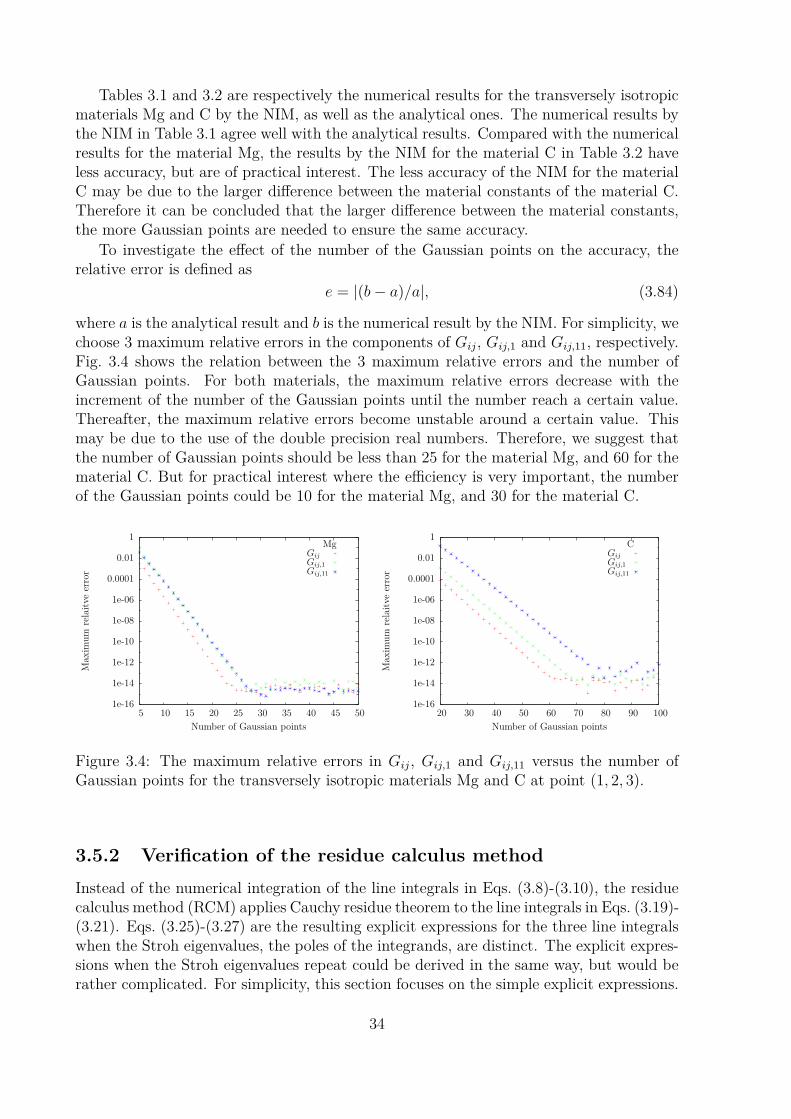
Tables 3.1 and 3.2 are respectively the numerical results for the transversely isotropicmaterials Mg and C by the NIM, as well as the analytical ones. The numerical results bythe NIM in Table 3.1 agree well with the analytical results. Compared with the numericalresults for the material Mg, the results by the NIM for the material C in Table 3.2 haveless accuracy, but are of practical interest. The less accuracy of the NIM for the materialC may be due to the larger difference between the material constants of the material C.Therefore it can be concluded that the larger difference between the material constants,the more Gaussian points are needed to ensure the same accuracy.

To investigate the effect of the number of the Gaussian points on the accuracy, therelative error is defined as

e = |(b− a)/a|, (3.84)

where a is the analytical result and b is the numerical result by the NIM. For simplicity, wechoose 3 maximum relative errors in the components of Gij, Gij,1 and Gij,11, respectively.Fig. 3.4 shows the relation between the 3 maximum relative errors and the number ofGaussian points. For both materials, the maximum relative errors decrease with theincrement of the number of the Gaussian points until the number reach a certain value.Thereafter, the maximum relative errors become unstable around a certain value. Thismay be due to the use of the double precision real numbers. Therefore, we suggest thatthe number of Gaussian points should be less than 25 for the material Mg, and 60 for thematerial C. But for practical interest where the efficiency is very important, the numberof the Gaussian points could be 10 for the material Mg, and 30 for the material C.

1e-16

1e-14

1e-12

1e-10

1e-08

1e-06

0.0001

0.01

1

5 10 15 20 25 30 35 40 45 50

Max

imum

rela

itve

erro

r

Number of Gaussian points

MgGijGij,1Gij,11

1e-16

1e-14

1e-12

1e-10

1e-08

1e-06

0.0001

0.01

1

20 30 40 50 60 70 80 90 100

Max

imum

rela

itve

erro

r

Number of Gaussian points

CGijGij,1Gij,11

Figure 3.4: The maximum relative errors in Gij, Gij,1 and Gij,11 versus the number ofGaussian points for the transversely isotropic materials Mg and C at point (1, 2, 3).

3.5.2 Verification of the residue calculus methodInstead of the numerical integration of the line integrals in Eqs. (3.8)-(3.10), the residuecalculus method (RCM) applies Cauchy residue theorem to the line integrals in Eqs. (3.19)-(3.21). Eqs. (3.25)-(3.27) are the resulting explicit expressions for the three line integralswhen the Stroh eigenvalues, the poles of the integrands, are distinct. The explicit expres-sions when the Stroh eigenvalues repeat could be derived in the same way, but would berather complicated. For simplicity, this section focuses on the simple explicit expressions.

34

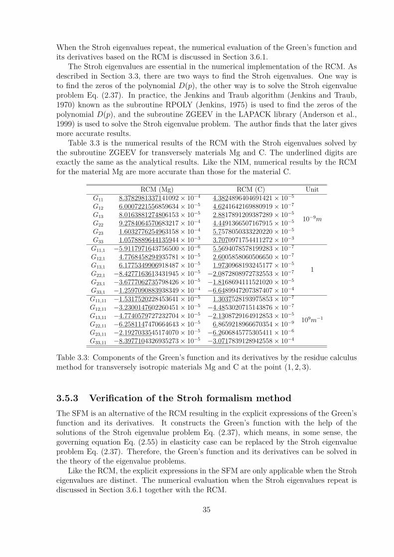
When the Stroh eigenvalues repeat, the numerical evaluation of the Green’s function andits derivatives based on the RCM is discussed in Section 3.6.1.

The Stroh eigenvalues are essential in the numerical implementation of the RCM. Asdescribed in Section 3.3, there are two ways to find the Stroh eigenvalues. One way isto find the zeros of the polynomial D(p), the other way is to solve the Stroh eigenvalueproblem Eq. (2.37). In practice, the Jenkins and Traub algorithm (Jenkins and Traub,1970) known as the subroutine RPOLY (Jenkins, 1975) is used to find the zeros of thepolynomial D(p), and the subroutine ZGEEV in the LAPACK library (Anderson et al.,1999) is used to solve the Stroh eigenvalue problem. The author finds that the later givesmore accurate results.

Table 3.3 is the numerical results of the RCM with the Stroh eigenvalues solved bythe subroutine ZGEEV for transversely materials Mg and C. The underlined digits areexactly the same as the analytical results. Like the NIM, numerical results by the RCMfor the material Mg are more accurate than those for the material C.

RCM (Mg) RCM (C) UnitG11 8.3782981337141092× 10−4 4.3824896404691421× 10−5

10−9m

G12 6.0007221556859634× 10−5 4.6241642169880919× 10−7

G13 8.0163881274806153× 10−5 2.8817891209387289× 10−5

G22 9.2784064570683217× 10−4 4.4491366507167915× 10−5

G23 1.6032776254963158× 10−4 5.7578050333220220× 10−5

G33 1.0578889644135944× 10−3 3.7070971754411272× 10−3

G11,1 −5.9117971643756500× 10−6 5.5694078578199283× 10−7

1

G12,1 4.7768458294935781× 10−5 2.6005858060506650× 10−7

G13,1 6.1775349906918487× 10−5 1.9730968193245177× 10−5

G22,1 −8.4277163613431945× 10−5 −2.0872808972732553× 10−7

G23,1 −3.6777062735798426× 10−5 −1.8168694111521020× 10−5

G33,1 −1.2597090883938349× 10−4 −6.6489947207387407× 10−4

G11,11 −1.5317520228453641× 10−5 1.3037528193975853× 10−7

109m−1

G12,11 −3.2300147602260451× 10−5 −4.4853020715143876× 10−7

G13,11 −4.7740579727232704× 10−5 −2.1308729164912853× 10−5

G22,11 −6.2581147470664643× 10−5 6.8659218966670354× 10−9

G23,11 −2.1927033545174070× 10−5 −6.2606845775305411× 10−6

G33,11 −8.3977104326935273× 10−5 −3.0717839128942558× 10−4

Table 3.3: Components of the Green’s function and its derivatives by the residue calculusmethod for transversely isotropic materials Mg and C at the point (1, 2, 3).

3.5.3 Verification of the Stroh formalism methodThe SFM is an alternative of the RCM resulting in the explicit expressions of the Green’sfunction and its derivatives. It constructs the Green’s function with the help of thesolutions of the Stroh eigenvalue problem Eq. (2.37), which means, in some sense, thegoverning equation Eq. (2.55) in elasticity case can be replaced by the Stroh eigenvalueproblem Eq. (2.37). Therefore, the Green’s function and its derivatives can be solved inthe theory of the eigenvalue problems.

Like the RCM, the explicit expressions in the SFM are only applicable when the Stroheigenvalues are distinct. The numerical evaluation when the Stroh eigenvalues repeat isdiscussed in Section 3.6.1 together with the RCM.

35

In the FORTRAN program, the Stroh eigenvalue problem is solved by the subroutineZGEEV in the LAPACK library. Table 3.4 contains the corresponding numerical resultsof the Green’s function and its derivatives for the materials Mg and C. The underlineddigits are exactly the same as the analytical solutions. The numerical results for thematerial C are less accurate than those for the material Mg. However, compared withthe results by the NIM and the RCM, the numerical results by the SFM for the materialC are more accurate. So the SFM are better at evaluating the Green’s function and itsderivatives for strongly anisotropic materials like C than the NIM and the RCM.

SFM (Mg) SFM (C) UnitG11 8.3782981337134370× 10−4 4.3827896251658357× 10−5

10−9m

G12 6.0007221557027949× 10−5 4.6263216287962473× 10−7

G13 8.0163881274811818× 10−5 2.8820815639255452× 10−5

G22 9.2784064570692107× 10−4 4.4521844547125352× 10−5

G23 1.6032776254961957× 10−4 5.7641631278404827× 10−5

G33 1.0578889644135981× 10−3 3.7072624469392723× 10−3

G11,1 −5.9117971638054452× 10−6 5.5707858596426121× 10−7

1

G12,1 4.7768458294993996× 10−5 2.6022661806317575× 10−7

G13,1 6.1775349906884700× 10−5 1.9731677300777066× 10−5

G22,1 −8.4277163614110222× 10−5 −2.0915785653823394× 10−7

G23,1 −3.6777062735840134× 10−5 −1.8178276707770339× 10−5

G33,1 −1.2597090883943480× 10−4 −6.6490424049476117× 10−4

G11,11 −1.5317520185524825× 10−5 1.3033886315670495× 10−7

109m−1

G12,11 −3.2300147619145314× 10−5 −4.4956207299378750× 10−7

G13,11 −4.7740579505173436× 10−5 −2.1314880907310438× 10−5

G22,11 −6.2581146860816642× 10−5 6.7320118850785253× 10−9

G23,11 −2.1927033538643924× 10−5 −6.2732112011148431× 10−6

G33,11 −8.3977103691742081× 10−5 −3.0719075049768016× 10−4

Table 3.4: Components of the Green’s function and its derivatives by the Stroh formalismmethod for transversely isotropic materials Mg and C at the point (1, 2, 3).

3.5.4 Verification of the unified explicit expressionsThe UEEM is based on the RCM. The explicit expressions by the UEEM are in terms ofthe Stroh eigenvalues. Although the expressions by the UEEM are more complicated thanthose by the RCM, they are applicable not only when the Stroh eigenvalues are distinctbut also when they repeat.

For the Green’s function, the explicit expressions in the UEEM is a straightforwardreformulation of those in the RCM. Ting and Lee (1997) presented the unified explicitexpression of the Green’s function for the first time. It is easy to find out that our newexplicit expression of the Green’s function is equivalent to that proposed by Ting and Lee(1997). Very recently, Buroni and Saez (2013) presented unified or unique explicit expres-sions for the derivatives of Green’s function by taking the derivatives of the expression ofGreen’s function by Ting and Lee (1997).

In the FORTRAN program, the Stroh eigenvalues are obtained by solving the Stroheigenvalue problem Eq. (4.1). Table 3.5 contains the numerical results of the Green’s

36

function and its derivatives by the UEEM for materials Mg and C. The underlined digitsagree well with the analytical solutions. In the Table 3.5, the number of underlineddigits for the material C is almost equal to that for the material Mg, where the numberof underlined digits for material C is significantly less than that for material Mg. Thisimplies that compared with the NIM, the RCM and the SFM, the UEEM has the mostadvantage of accuracy in computing the Green’s function and its derivatives for stronglyanisotropic materials.

UEEM (Mg) UEEM (C) UnitG11 8.3782981337130402× 10−4 4.3827896221260154× 10−5

10−9m

G12 6.0007221557104867× 10−5 4.6263223755486468× 10−7

G13 8.0163881274800475× 10−5 2.8820815639128454× 10−5

G22 9.2784064570696130× 10−4 4.4521844577592456× 10−5

G23 1.6032776254960092× 10−4 5.7641631278256841× 10−5

G33 1.0578889644135964× 10−3 3.7072624469392710× 10−3

G11,1 −5.9117971638177865× 10−6 5.5707948825936864× 10−7

1

G12,1 4.7768458294984333× 10−5 2.6022823188120584× 10−7

G13,1 6.1775349906880689× 10−5 1.9731677292333828× 10−5

G22,1 −8.4277163614102633× 10−5 −2.0915875780597619× 10−7

G23,1 −3.6777062735839781× 10−5 −1.8178276693589039× 10−5

G33,1 −1.2597090883943341× 10−4 −6.6490424049481234× 10−4

G11,11 −1.5317520185560367× 10−5 1.3037961156922419× 10−7

109m−1

G12,11 −3.2300147619146337× 10−5 −4.4871709610018432× 10−7

G13,11 −4.7740579505166646× 10−5 −2.1314882684264957× 10−5

G22,11 −6.2581146860783736× 10−5 6.6917582325344854× 10−9

G23,11 −2.1927033538653885× 10−5 −6.2732119813698278× 10−6

G33,11 −8.3977103691742231× 10−5 −3.0719075049293141× 10−4

Table 3.5: Components of the Green’s function and its derivatives by the unified explicitexpression method for transversely isotropic materials Mg and C at the point (1, 2, 3).

3.5.5 Comparison of the efficiencyBefore the general evaluations of the Green’s function and its derivatives by the fourmethods, a comparison of the four methods on the efficiency is presented first.

The FORTRAN programs of the four different methods are implemented under thesame computing environment. Fig. 3.5 is a comparison of the computing time required bythe four methods. The material is Mg, and the evaluation point is (1, 2, 3)m. The numberof the Gaussian points in the NIM is set to be 25 for a comparable accuracy with the othermethods. The bottom box of each method represents the computing time for the Green’sfunction including the time for the Gaussian points and the weights in the NIM, the Stroheigenvalues in the RCM and the UEEM, and the eigenvalues and eigenvectors of N in theSFM. The middle box represents the additional computing time for the first derivative ofthe Green’s function excluding the time for the Green’s function. The total computingtime for the second derivative of the Green’s function is represented by the three boxes,i.e., the stacked column. From Fig. 3.5, the explicit methods, namely the RCM, the SFMand the UEEM, have a higher efficiency for computing the Green’s function and its firstderivative compared to the NIM, but may lose the advantage for computing the secondderivative of the Green’s function, especially, in the RCM and the SFM. Both the RCM

37

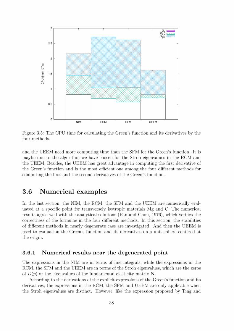
0

0.5

1

1.5

2

2.5

3

NIM RCM SFM UEEM

CP

U tim

e (

10

-4s)

GijGij,kGij,kl

Figure 3.5: The CPU time for calculating the Green’s function and its derivatives by thefour methods.

and the UEEM need more computing time than the SFM for the Green’s function. It ismaybe due to the algorithm we have chosen for the Stroh eigenvalues in the RCM andthe UEEM. Besides, the UEEM has great advantage in computing the first derivative ofthe Green’s function and is the most efficient one among the four different methods forcomputing the first and the second derivatives of the Green’s function.

3.6 Numerical examplesIn the last section, the NIM, the RCM, the SFM and the UEEM are numerically eval-uated at a specific point for transversely isotropic materials Mg and C. The numericalresults agree well with the analytical solutions (Pan and Chou, 1976), which verifies thecorrectness of the formulae in the four different methods. In this section, the stabilitiesof different methods in nearly degenerate case are investigated. And then the UEEM isused to evaluation the Green’s function and its derivatives on a unit sphere centered atthe origin.

3.6.1 Numerical results near the degenerated pointThe expressions in the NIM are in terms of line integrals, while the expressions in theRCM, the SFM and the UEEM are in terms of the Stroh eigenvalues, which are the zerosof D(p) or the eigenvalues of the fundamental elasticity matrix N.

According to the derivations of the explicit expressions of the Green’s function and itsderivatives, the expressions in the RCM, the SFM and UEEM are only applicable whenthe Stroh eigenvalues are distinct. However, like the expression proposed by Ting and

38

Lee (1997), the explicit expressions in the UEEM are assumed to be applicable when theStroh eigenvalues repeat which will be proved by the numerical examples.

Since the expressions are dependent on the Stroh eigenvalues, here we give a study onthe Stroh eigenvalues for transversely isotropic materials whose symmetry axis is alongwith the x3-axis. When ξ is defined in Eq. (3.16)1, the zeros of D(p) are equal to thoseof D(ξ). The expression of D(ξ) is (Mura, 1987)

D(ξ) =(α′η2 + γξ2

3

) αγη4 +

(αβ + γ2 − γ′2

)η2ξ2

3 + βγξ43

, (3.85)

where

α = C11 = C22, α′ = C66 = (C11 − C12) /2,β = C33, γ′ − γ = C13 = C23, (3.86)γ = C44 = C55, η2 = ξ2

1 + ξ22 .

Generally, the zeros of Eq. (3.85) are three distinct pairs of complex conjugates, i.e.,three distinct Stroh eigenvalues. But the Stroh eigenvalues repeat when x = (0, 0, a), a 6=0. When x = (0, 0, a), a 6= 0, the corresponding n and m can be arbitrarily chosen as

n = (cos θ, sin θ, 0), m = (− sin θ, cos θ, 0), (3.87)

where θ is a parameter in the plane x3 = 0. Substitution of Eq. (3.87) into Eq. (3.16)1yields

ξ3 = 0, η2 = cos2 ψ(1 + p2). (3.88)

Furthermore, substitution of Eq. (3.88) into Eq. (3.85) leads to the unique zeros p = ±i,which means the three Stroh eigenvalues are identical or fully degenerated when x =(0, 0, a).

To investigate the abilities of the expressions in the NIM, the RCM, the SFM and theUEEM in dealing with the degenerate and nearly degenerate cases, a numerical evalua-tion of the four methods near the fully degenerated point (0, 0, 1) is performed. For thenumerical examples, the material is taken as the transversely isotropic material Mg, andthe evaluation points are x = (0, sin θ, cos θ) near θ = 0.

Fig. 3.6 is the numerical results of a component of the Green’s function evaluated bythe expressions in the NIM, the RCM, the SFM and the UEEM for the material Mg nearthe point x = (0, 0, 1). The results evaluated by the NIM, the SFM and the UEEM arealmost the same even at the degenerated point (when θ = 0). But the results evaluatedby the RCM become unstable near the degenerated point. Therefore, the applicability ofthe expressions in the SFM and the UEEM for the Green’s function in degenerate andnearly degenerate cases is confirmed but not the expression in the RCM. The numericalerrors of the explicit expression in the RCM may be due to the items like (pi − pj) indenominators, which is close to zero in the nearly degenerate cases.

Fig. 3.7 is the numerical results of G33,2 evaluated by the expressions in the fourmethods for the transversely isotropic matherial Mg near the degenerate point. Theresults evaluated by the NIM and the UEEM still agree perfectly with each other, evenat the degenerate point. In the RCM, significant errors arise when θ < 1.5, moreover thenumerical errors are too large to plot the results in the figure near the area very close tothe degenerate point. In the SFM, numerical errors arise when θ < 0.1. The numerical

39

-0.005

0

0.005

0.01

0.015

0.02

0 0.01 0.02 0.03 0.04 0.05

G33

(m)

θ (degree)

NIMRCMSFM

UEEM

Figure 3.6: Numerical evaluations of the Green’s function around the denegerated pointfor the transversely isotropic material Mg

-5

-4

-3

-2

-1

0

0 1 2 3 4 5

G33

,2

θ (degree)

NIMRCMSFM

UEEM

-9×10-5-8×10-5-7×10-5-6×10-5-5×10-5-4×10-5-3×10-5-2×10-5-1×10-5

0

0 0.1 0.2 0.3 0.4 0.5

Figure 3.7: Numerical evaluations of the first derivatvie of the Green’s function aroundthe denegerated point for the transversely isotropic material Mg

40

-30

-25

-20

-15

-10

-5

0

5

0 5 10 15 20 25 30

G33

,22

(m-1

)

θ (degree)

NIMRCMSFM

UEEM

-0.05

0

0.05

0.1

0.15

0.2

0.25

0.3

0 0.1 0.2 0.3 0.4 0.5

Figure 3.8: Numerical evaluations of the second derivatvie of the Green’s function aroundthe denegerated point for the transversely isotropic material Mg

errors in the SFM may also come from the items like (pi − pj) in the denominators. Butthe error area in the SFM is about 6.67% of that in the RCM.

Fig. 3.8 is the numerical results of G33,22 evaluated by the expressions in the fourmethods for the transversely isotropic material Mg near the degenerate point. The resultsevaluated by the NIM and the UEEM agree perfectly with each other. But the numericalerrors arise near the degenerate point in both the RCM and the SFM. The error area inthe evaluation of G33,22 by the RCM is about θ < 8 which is about 5.3 times of the errorarea in the evaluation of G33,2 by the RCM. The error area of the second derivative G33,22in the SFM is similar with that of the first derivative G33,2 in the SFM, and is about1.25% of that in the RCM.

Through the above numerical evaluations, it may be concluded on the three explicitmethods that

1. The expressions of the Green’s function and its derivatives in the UEEM and theexpression of the Green’s function in the SFM may be applicable no matter theStroh eigenvalues are distinct or not.

2. The expressions of the Green’s function and its derivatives in the RCM and theexpression of the derivatives of the Green’s function in the SFM are only applicablewhen the Stroh eigenvalues are distinct (the non-degenerate case). They fail whenthe Stroh eigenvalues repeat (the degenerate case) and cause significant numericalerrors at the area very close to the degenerated point (the nearly degenerate case).

3. The SFM is more stable than the RCM near the fully degenerate cases.

Besides, although the RCM and the SFM are not applicable in the degenerate andnearly-degenerate cases, they are still of practical interest as long as the Stroh eigenvalues

41

keep distinct by using some numerical techniques, For example, a small perturbation suchas 10−6 on some material constants.

3.6.2 Numerical results for an arbitrary point on a unit sphereAs the previous sections reveal, compared to the other three methods, the UEEM has themost advantage in the numerical evaluation of the Green’s function and its derivativesfor 3D anisotropic materials. In this section, the Green’s function and its derivatives on aunit sphere are evaluated by the UEEM. The evaluation points on the upper half sphereare denoted by (cos θ cosφ, cos θ sinφ, sin θ) with φ ∈ (0, 2π) and θ ∈ (0, π). The geometryof the sphere is illustrated by Fig. 3.9. The material is the transversely isotropic material

x

1

1

1

x3

x2

x1

𝜃

𝜙

Figure 3.9: Spherical coordinates of the field point x

Mg. Figs. 3.10-3.12 are respectively the numerical results of the Green’s function, its firstderivative and its second derivative on the upper half sphere, and the contours of theGreen’s function and its derivatives are presented on the base planes of the coordinatesystems. It is observed that the periods of the Green’s function and its derivatives are πin θ, and 2π in φ, while for some components may be π in φ.

Similar figures can be plotted by the NIM. In order to give the similar figures by theRCM and the SFM, a small perturbation of the material constants is required to keepthe Stroh’s eigenvalues distinct so that the explicit expressions can be used for practicalinterest.

3.7 Concluding remarksFour different methods for computing the Green’s function and its first and second deriva-tives are presented in this chapter. The Green’s function and its derivatives are expressed

42

G11(10-3m)

0π

θπ2π

ϕ

3

4

G22(10-3m)

0π

θπ2π

ϕ

3

4

G33(10-3m)

0π

θπ2π

ϕ

3 4

G12(10-4m)

0π

θπ2π

ϕ

-5

5

G13(10-4m)

0π

θπ2π

ϕ

-5

5

G23(10-4m)

0π

θπ2π

ϕ

-5

5

Figure 3.10: General evaluation of the anisotropic elastic Green’s function by the UEEM.

G11,1(10-3)

0π

θπ2π

ϕ

-3

3

G22,1(10-3)

0π

θπ2π

ϕ

-3

3

G33,1(10-3)

0π

θπ2π

ϕ

-3

3

G12,1(10-4)

0π

θπ2π

ϕ

-7 7

G13,1(10-4)

0π

θπ2π

ϕ

-7

7

G23,1(10-4)

0π

θπ2π

ϕ

-5

5

Figure 3.11: General evaluation of the first derivative of the anisotropic elastic Green’sfunction by the UEEM.

43

G11,11(10-3m-1)

0π

θπ2π

ϕ

-1 4

G22,11(10-3m-1)

0π

θπ2π

ϕ

-4 4

G33,11(10-3m-1)

0π

θπ2π

ϕ

-6

4

G12,11(10-3m-1)

0π

θπ2π

ϕ

-3

3

G13,11(10-3m-1)

0π

θπ2π

ϕ

-3

3

G23,11(10-3m-1)

0π

θπ2π

ϕ

-1.5

1.5

Figure 3.12: General evaluation of the second derivative of the anisotropic elastic Green’sfunction by the UEEM.

in terms of three line integrals. The line integral expressions are a little different fromthe conventional line integral expressions of the 3D anisotropic Green’s function and itsderivatives, especially for the second derivative of the Green’s function where the sym-metry of some tensors is used to simplify it. The first method (NIM) is straightforwardlybased on the numerical integration of the line integrals. The second method (RCM) isbased on the explicit expressions derived by applying the residue calculus with the dis-tinctness assumption of the Stroh eigenvalues to the line integrals. The integrals in thefirst and second methods are the same. In the third method (SFM), the Green’s functionand its derivatives are constructed from the solutions of a six-dimensional formulationof an eigenvalue problem. In the fourth method (UEEM), the line integrals are firstlyexpressed in terms of two elementary line integrals, and then evaluated by the simple poleresidue calculus followed by a rewritten of the resulting explicit expressions. Althoughthe explicit expressions in the UEEM are derived with the distinctness assumption ofthe Stroh eigenvalues, after the rewritten they are applicable when the Stroh eigenvaluesrepeat. The correctness of the expressions in the four methods is confirmed by comparingthe numerical results of the Green’s function and its derivatives for transversely isotropicmaterials at an arbitrary point with the analytical results. The numerical results of theRCM and the SFM near a degenerate point may become unstable, while the NIM andUEEM remain applicable near and at the degenerate point. According to the CPU timesused by the four different methods to calculate the Green’s function and its derivatives,the UEEM seems to be the most efficient one.

44

Chapter 4

Green’s function in linearpiezoelectricity

4.1 Problem statementIn linear elasticity, the 3D anisotropic Green’s function has been well studied. It wasfirst investigated by Fredholm (1900). There are now many methods to evaluate theGreen’s function, among which we only mention the numerical integration method, theresidue calculus method and the Stroh formalism method (Fredholm, 1900; Malen, 1971).To calculate the derivatives of the 3D anisotropic elastic Green’s function, Malen (1971)used the Stroh formalism method, Barnett (1972) used the numerical integration method,and Sales and Gray (1998) used the residue calculus method. The last two methods werebased on the line integral expressions. Both the Stroh formalism and the residue calculusmethods can lead to explicit expressions of the 3D anisotropic elastic Green’s functionand its derivatives. The residue calculus method has been further investigated by Tingand Lee (1997), Phan et al. (2004, 2005), Lee (2003, 2009), Buroni and Saez (2013) andXie et al. (2013) among others.

However, in contrast to the 3D anisotropic elastic Green’s function and its derivatives,relatively few studies can be found in the literature on the 3D anisotropic piezoelectricGreen’s function and its derivatives. For transversely isotropic piezoelectric materials,Dunn and Wienecke (1996) and Ding et al. (1996) derived the analytical expression of theGreen’s function, while Soh et al. (2003) presented 3D Green’s function for transverselyisotropic magnetoelectroelastic solids. In contrast, the 3D Green’s function and its deriva-tives for generally anisotropic piezoelectric materials are very complicated and have noanalytical expressions known in literature. Deeg (1980) derived the Green’s function interms of line integrals by using Radon transform. Chen (1993) and Chen and Lin (1993)derived the Green’s function and its derivatives as line integrals by Fourier transform andthen computed them by numerical integration. Dunn (1994) and Pan and Tonon (2000)obtained the Green’s function by applying the residue calculus method to the infinite lineintegrals. And the later also evaluated the first derivative of the Green’s function by afinite difference scheme. By using the Stroh formalism method, Akamatsu and Tanuma(1997) gave an explicit expression for the 3D anisotropic piezoelectric Green’s functionbut not its derivatives. The advantage of the Stroh formalism and the residue calcu-lus methods is that they give rise to explicit expressions instead of integral expressions.Though the residue calculus method was used to derive the Green’s function and its first

45

and second derivatives for magneto-electro-elastic solids by Buroni and Saez (2010), nonumerical results of the second derivative were presented. An excellent monograph onstatic Green’s functions in anisotropic media was recently published by Pan and Chen(2015), and interested readers may find a detailed review, comprehensive references andmany new results in this monograph.

In this Chapter, explicit expressions for the Green’s function and its first and secondderivatives in 3D anisotropic piezoelectricity are derived by both the Stroh formalismmethod and the residue calculus method. In the Stroh formalism method, the approachto calculate the derivatives of the eigenvectors proposed by Nelson (1976) is used to derivethe explicit expressions for the derivatives of the Green’s function. In the residue calculusmethod, line integral expressions of the Green’s function and its derivatives are obtainedby generalizing the elastic results of Mura (1987), which are subsequently evaluated byusing the Cauchy’s residue theorem. Different from the expressions given by Lee (2003),the present integral expressions are easy to evaluate, especially for the second derivativeof the Green’s function, since they do not involve tensors higher than 4th-order. Theexplicit expressions obtained by both methods are coded into FORTRAN programs. Theaccuracy and the efficiency of both methods are compared with each other by numericalexamples.

The contributions in the chapter have be published in

• L. Xie, C. Zhang, C. Hwu, J. Sladek, V. Sladek, On two accurate methods for com-puting 3D Green’s function and its first and second derivatives in piezoelectricity,Engineering Analysis with Boundary Elements, 61:183-193, 2015.

4.2 Stroh formalism methodThe generalized displacement Green’s function GIJ(x) is governed by the equation (2.55)in piezoelectricity case.

The Green’s function GIJ(x) (I, J = 1, 2, . . . , 4) denotes the mechanical displacementat x in the xI-direction (I ≤ 3) or the electric potential (I = 4) when a unit point force atthe origin in the xJ -direction (J ≤ 3), or a unit point charge at origin (J = 4) is applied.Besides, the Green’s function and its derivatives vanish when |x| → ∞.

Malen (1971) showed that the Green’s function in 3D linear elasticity can be expressedin terms of the solution of an eigensystem, which is known as the Stroh eigen-relation. Sothe Green’s function in piezoelectric solids could be expressed in terms of the solution ofthe Stroh eigen-relation in piezoelectricity.

4.2.1 Representation of the Green’s functionThe Stroh eigen-relation or the Stroh eigenvalue problem at a point x in a piezoelectricsolid with the material constants ckIJl is given by a 8-dimensional eigensystem as (Hwu,2010)

Nξ = pξ, (4.1a)

in which

N =(

N1 N2N3 NT

1

), ξ =

ab

, (4.1b)

46

N1 = −T−1RT , N2 = T−1 = NT2 , N3 = RT−1RT −Q,

andQIJ = ckIJlnknl, RIJ = ckIJlnkml, TIJ = ckIJlmkml, (4.1c)

where n and m are two mutually orthogonal unit vectors on the oblique plane perpen-dicular to x. Since N is not symmetric, ξ in Eq. (4.1a) is a right eigenvector. The lefteigenvector denoted by η satisfies

ηTN = pηT , (4.2)

where Ting (1996) had proved that

η =ba

. (4.3)

It can be shown that the eigenvalues of Eq. (4.1a) are four pairs of complex con-jugates (Akamatsu and Tanuma, 1997). It is assumed that Im(pk) > 0, pk+4 = pk,k = 1, 2, 3, 4 and pk are distinct which causes that all the eigenvectors are independent ofeach other.

By definingA = [a1,a2,a3,a4] , B = [b1, b2, b3, b4] , (4.4)

and with the relation between the eigenvectors

ηTαξβ = δαβ, α, β = 1, 2, . . . , 8, (4.5)

where δαβ is the Kronecker delta, the Green’s function can be expressed as

G(x) = 14πrH(x), H = 2iAAT , (4.6)

in which r = |x|, x is the unit vector of x, and H is one of the three Barnett-Lothematrices in linear piezoelectricity. The explicit expression of A can be found in Hwu(2010), and is listed in Appendix D for the completeness.

4.2.2 First derivative of the Green’s functionThe first derivative of the Green’s function becomes straightforward by differentiatingEq. (4.6) with respect to xi, i.e.,

G,i(x) = 14πr2

(−xir

H + rH,i

), (4.7a)

where

H,i = 2i(A,iAT +

[A,iAT

]T). (4.7b)

According to the above equations, the first derivatives of A is required to calculate thederivative of G(x). All components of A and its derivatives in 3D linear elasticity canbe expressed explicitly in terms of the Stroh eigenvalues (Hwu, 2010), So the derivativesof A can be obtained by taking the derivatives of all the components. However the

47

expressions would be too complex. In the following we present an alternative way to getthe derivatives of A for 3D linear piezoelectric materials.

Taking the derivative of Eq. (4.1a), which is associated with the eigenvalue pα and thecorresponding right eigenvector ξα, with respect to xi leads to


Note that the repeated Greek indices in the above equation do not imply summation, neitherdo in the following. Since the derivative of an eigenvector is an 8-dimensional vector, itis a linear combination of the 8 independent eigenvectors, i.e.,

ξα,i =8∑

β=1c

(i)αβξβ, (4.9a)

andηα,i =

8∑β=1

c(i)αβηβ. (4.9b)

In Eq. (4.9), the coefficients c(i)αβ are constants. In virtue of Eqs. (4.1a), (4.2) and (4.5),

the substitution of Eq. (4.9a) into Eq. (4.8) followed by the premultiplication by ηTβ gives

c(i)αβ(pβ − pα) = −ηTβ (N,i − pα,iI)ξα. (4.10)

When β = α, the derivative of the eigenvalue pα is given from Eq. (4.10) as


If β 6= α the coefficients c(i)αβ in the expressions of the derivatives of the eigenvectors ξα,i

are given by

c(i)αβ =


. (4.12)


c(i)αβ + c

(i)βα = 0. (4.13)


So far, all the coefficients c(i)αβ are determined. The first derivative of the eigenvector

can be expressed in terms of all eigenvectors by Eq. (4.9). And one further easily arrivesat A,i by differentiating Eq. (4.4). The explicit expressions of the N,i are presented inAppendix B. It should be mentioned that different explicit expressions of the derivativesof the anisotropic elastic Green’s function were investigated by Lavagnino (1995).

4.2.3 Second derivative of the Green’s functionThe second derivative of the Green’s function is obtained by taking derivative of Eq. (4.7)with respect to xj, i.e.,

G,ij(x) = 14πr3

[(3xixjr2 − δij


], (4.15a)

48

where

H,ij = 2i(A,ijAT + A,iAT

,j +[A,ijAT + A,iAT

,j

]T). (4.15b)

In order to get the second derivative of A, the second derivative of the right eigenvec-tors ξα,ij is required. In the same way, ξα,ij is a linear combination of the 8 independentright eigenvectors as

ξα,ij =8∑

β=1d

(ij)αβ ξβ. (4.16)

Taking the derivative of Eq. (4.8) with respect to xj followed by the premultiplication byηTβ with the substitution of Eq. (4.16) yields

d(ij)αβ (pβ − pα) = −ηTβ (N,ij − pα,ijI)ξα − ηTβ (N,i − pα,iI)ξα,j − ηTβ (N,j − pα,jI)ξα,i. (4.17)

Using the same approach for the first derivative of the eigenvectors, the second derivativeof the eigenvalues pα,ij and the coefficients d(ij)

αβ are

pα,ij = ηTαN,ijξα + ηTαN,iξα,j + ηTαN,jξα,i, (4.18)d(ij)αα = −(ηTα,iξα,j + ηTα,jξα,i)/2, (4.19)

d(ij)αβ =


, β 6= α. (4.20)

In Eqs. (4.18)-(4.20), N,i and N,ij can be straightforwardly obtained by taking thederivatives of Eqs. (4.1b) and (4.1c). Appendix B presents the explicit expressions of N,ij

as well as the proper choice of n, m and their derivatives.

4.3 Residue calculus methodSince the Green’s function can be reduced to a line integral, it is straightforward toevaluate the Green’s function by using the Cauchy’s residue theorem. In this section, weintroduce this alternative method.

4.3.1 Representation of the Green’s functionEq. (2.55) in piezoelectricity case can be solved by using either Fourier transform or Radontransform (Qin, 2010). The Green’s function can be expressed by an area integral as

GIJ(x) = 18π2

∫S2δ(ξ · x)K−1

IJ (ξ)dS(ξ), (4.21)

where ξ is a parameter vector, S2 is the surface of the unit sphere in the ξ-space andKIJ(ξ) = ckIJlξkξl with the symmetry relation KIJ = KJI .

Further, the area integral can be reduced to be a line integral over a unit circle as

GIJ(x) = 18π2r

∮SK−1IJ (ξ)dφ, (4.22)

49

where S is the unit circle on the oblique plane perpendicular to x and φ is a parameterin the oblique plane.

To get the explicit expressions of the Green’s function, the line integrals over the unitcircle are transformed into improper integrals from −∞ to +∞. By choosing any twomutually orthogonal unit vectors n and m on the oblique plane as the bases, ξ can bewritten as

ξ = n cosφ+m sinφ, (4.23)

where φ is the angle between n and ξ. Setting

p = tanφ, ξ∗ = n+ pm, (4.24)

we haveξ = cosφ ξ∗, dφ = cos2 φdp. (4.25)

Substituting Eq. (4.25) into Eqs. (4.22), the Green’s function yields

GIJ(x) = 12πrAIJ(x), (4.26)

whereAIJ(x) = 1

2π

∫ +∞

−∞NIJ(p)D−1(p)dp. (4.27)

In Eqs. (4.27), NIJ(p) and D(p) are the cofactors and the determinant of KIJ(p) =ckIJlξ

∗kξ∗l , respectively.

D(p) is an 8th-order polynomial, which leads to eight roots with four pairs of complexconjugates. Note that n or m in the Stroh’s formalism method and the residue calculusmethod are not necessarily the same, but if they are chosen the same, the roots of D(p)are equal to the eigenvalues of the Stroh’s eigen-relation (4.1).

By now, the Green’s function is expressed in terms of an improper line integral, i.e.,Eq. (4.27). Since NIJ(p) is a 6th-order polynomial in p, the explicit expression of theGreen’s function can be obtained by applying Cauchy’s residue theorem on the improperline integral AIJ(x).

With distinctness assumption on the four pairs of the complex conjugates, the explicitexpression of AIJ(x) is given by

AIJ(x) = − Im4∑

n=1

NIJ(pn)D′(pn) , (4.28)

where the prime ′ denotes the derivative with respect to p and pn are the complex rootsof D(p) with positive imaginary parts. For details, the readers refer to Appendix A.

Therefore the explicit expression of the Green’s function is obtained by substitutingEq. (4.28) into Eq. (4.26).

4.3.2 First derivative of the Green’s functionDifferentiating Eq. (4.21) with respect to xk leads to the first derivative of the Green’sfunction as

GIJ,k(x) = 18π2

∫S2δ′(ξ · x)ξkK−1

IJ (ξ)dS(ξ), (4.29)

50

where the prime ′ denotes the derivative with respect to the argument, i.e., ξ · x.After some mathematical elementary manipulations, Eq. (4.29) can be recast into the

following line integrals over a unit circle as

GIJ,k(x) = 18π2r2

∮S

[−xkK−1

IJ (ξ)

+ ξkcpLMq(xpξq + ξpxq)K−1LI (ξ)K−1

MJ(ξ)]dφ. (4.30)

Similar equations as above for the elastic materials with detailed derivations were pre-sented by Mura (1987). For simplify, Eq. (4.30) can be rewritten as the following equation

GIJ,k(x) = 12πr2 [−xkAIJ(x) + PIJk(x)] , (4.31)

in which AIJ(x) is defined by Eq. (4.27) and

PIJk(x) = 12π

∫ +∞

−∞ξ∗kHIJ(p)D−2(p)dp, (4.32)

where HIJ(p) is given by

HIJ(p) = FIM(p)NJM(p), FIM(p) = EHM(p)NIH(p),FIM(p) = EHM(p)NIH(p). (4.33)

In Eq. (4.32) ξ∗i is a 1st-order polynomial in p and HIJ(p) is a 13th-order polynomialin p. Therefore following the derivation in Appendix A, the explicit expression of PIJk(x)is given by

PIJk(x) = − Im4∑

n=1

D′(pn)H ′IJk(pn)−D′′(pn)HIJk(pn)D′3(pn) , (4.34)

whereHIJk(p) = ξ∗kHIJ(p). (4.35)

The first derivative of the Green’s function is obtained by substituting Eqs. (4.28) and(4.34) into Eq. (4.31).

4.3.3 Second derivative of the Green’s functionThe second derivative of the Green’s function is given by taking the derivative of Eq. (4.29)with respect to xj, i.e.,

GIJ,kl(x) = 18π2

∫S2δ′′(ξ · x)ξkξlK−1

IJ (ξ)dS(ξ). (4.36)

After some manipulations (Mura, 1987), the second derivative of the Green’s functionbecomes

GIJ,kl(x) = 14π2r3

∮S

xkxlK

−1IJ (ξ)− [(xkξl + ξkxl)(xpξq + ξpxq) + ξkξlxpxq]

× cpHMqK−1IH(ξ)K−1

JM(ξ) + ξkξlcpHMq(xpξq + ξpxq)caSTb(xaξb + ξaxb)×K−1

JM(ξ)K−1IS (ξ)K−1

HT (ξ)dφ, (4.37)

51

Note that Eq. (4.37) is a little different from the corresponding equation by Mura (1987)for the elastic materials, since the symmetry relations of ciJMn and KIJ are used. FurtherEq. (4.37) can be recast into the following equation

GIJ,kl(x) = 1πr3 AIJ(x)xkxl − [PIJk(x)xl + PIJl(x)xk] +QIJkl(x) , (4.38)

where AIJ(x) is defined by Eq. (4.27), PIJk(x) is defined by Eq. (4.32), and QIJkl(x) isdefined by

QIJkl(x) = 12π

∫ +∞

−∞ξ∗kξ∗lMIJ(p)D−3(p)dp, (4.39)

in which MIJ(p) is given by

MIJ(p) = LIJ(p)−RIJ(p)D(p), LIJ(p) = FJH(p)HIH(p),RIJ(p) = xpxqCpHMqNIH(p)NJM(p). (4.40)

Since MIJ(p) is a 20th-order polynomial in p, following the derivation in Appendix A,the explicit expression of QIJkl(x) is given by

QIJkl(x) =− Im4∑

n=1

12D′5(pn)

D′2(pn)M ′′

IJkl(pn)− 3D′(pn)D′′(pn)M ′IJkl(pn)

+[3D′′2(pn)−D′′′(pn)D′(pn)

]MIJkl(pn)

, (4.41)

whereMIJkl(p) = ξ∗kξ

∗lMIJ(p). (4.42)

Here, MIJkl(p) is a polynomial of 22th-order respectively.Since D(p), HIJk(p) and MIJkl(p) are polynomials, they and their derivatives can be

calculated almost exactly by proper algorithms for polynomials.Finally, the second derivative of the Green’s function is obtained by substituting

Eqs. (4.28), (4.34) and (4.41) into Eq. (4.38).

4.4 Numerical proceduresThe numerical procedure for each of the two methods can be divided into four steps. Inthe SFM, the four steps are:

i) Determination of n, m and their derivatives.n and m can be any two mutually orthogonal unit vectors on the oblique planeperpendicular to the given position vector x. In our analysis n and m are chosenas Eq. (B.6) or Eq. (B.10), and their derivatives are evaluated correspondingly byEq. (B.9) or Eq. (B.11).

ii) Determination of the Stroh fundamental piezoelectricity matrix N and its derivatives.N is determined by Eq. (4.1). The derivatives of N can be derived from Eq. (4.1)and the derivatives of n and m.

52

iii) Computation of the eigenvalues pα, the right eigenvectors ξα and their derivatives.In our analysis, the subroutine ZGEEV in LAPACK library (Anderson et al., 1999)is used to calculate pα and ξα. Eqs. (4.9a) and (4.11) are used to calculate the firstderivatives of ξα and pα. Eqs. (4.16) and (4.18) are used to calculate the secondderivatives of ξα and pα.

iv) Computation of GIJ(x), GIJ,k(x) and GIJ,kl(x).The Green’s function and its derivatives are computed by Eqs. (4.6), (4.7) and (4.15).For this purpose, ξα and their derivatives are used to construct A and its derivatives.

In the RCM, the four steps are:

i) Determination of n and m.There is no need to calculate the derivatives of n and m. In our method, n and mare chosen as (B.6) or (B.10).

ii) Computation of the Stroh eigenvalues pk (k = 1, 2, 3, 4).The eigenvalues pk are zeros of the polynomial D(p), which is the determinant ofKIJ(p) = ckIJlξ

∗kξ∗l with ξ∗ = n + pm. Many algorithms can be used to find the

zeros of D(p). In our method, we use the same algorithm as in the SFM to findpk (k = 1, 2, 3, 4), since the zeros of the polynomial D(p) are equal to the eigenvaluesof N if n and m are the same.

iii) Evaluation of NIJ(p), D(p), HIJk(p), MIJkl(p) and their derivatives.Because NIJ(p), D(p), HIJk(p) and MIJkl(p) are polynomials, their coefficients canbe determined in an accurate way by using the suitable algorithms for polynomialsin a computer program.

iv) Computation of GIJ(x), GIJ,k(x) and GIJ,kl(x).The Green’s function and its derivatives can be determined by AIJ(x), PIJk(x) andQIJkl(x) with Eqs. (4.26), (4.31) and (4.38). The Green’s function GIJ(x) is de-termined by AIJ(x) only. Additionally, PIJk(x) is required to determine the firstderivative of the Green’s function GIJ,k(x). And the second derivative of the Green’sfunction GIJ,kl(x) is determined by AIJ(x), PIJk(x) and QIJkl(x), which are definedby Eqs. (4.28), (4.34) and (4.41), respectively.

It should be mentioned that the Green’s function can be evaluated without assuming thedistinctness of the eigenvalues pα of N, also known as the Stroh eigenvalues (Akamatsuand Tanuma, 1997), but according to Eqs. (4.12) and (4.20) the distinctness assumptionis necessary to evaluate the derivatives of the Green’s function in the SFM. However,the distinctness of the Stroh eigenvalues is required in the RCM for both the Green’sfunction and its derivatives. Hence, for the cases with repeated Stroh eigenvalues, a smallperturbation on the material constants is suggested to avoid repeated or degeneratedeigenvalues in the RCM.

4.5 Numerical examples and discussionsThe transversely isotropic piezoelectric material, Lead Zirconate Titanate (PZT), is usedin the numerical examples. Choosing the axis of the material symmetry as the x3-axis,

53

the non-zero components of the elasticity tensor Cijkl in contracted notation are given by

C11 = C22 = 139, C12 = 77.8, C13 = C23 = 74.3, (4.43)C33 = 115, C44 = C55 = 25.6, C66 = 30.6,

(unit: 109N/m2

)The non-zero components of the piezoelectric constants enij in contracted notation are

e31 = e32 = −5.1, e33 = 15.1, e24 = e15 = 12.7, (unit: C/m) , (4.44)

and the non-zero components of the dielectric constants κin are

κ11 = κ22 = 6.461, κ33 = 5.620,(unit: 10−9C/(Vm)

). (4.45)

The source of the Green’s function is located at the origin of the Cartesian coordinatesystem and the observation point is arbitrarily chosen as (1, 2, 3).

In order to compare the numerical results with the analytical results, the analyticalsolution for transversely isotropic piezoelectric material presented by Ding et al. (1996) isevaluated by MATHEMATICA to give the exact results of the Green’s function and itsderivatives. The SFM is implemented in double precision and the RCM is implementedin quadruple precision to have a similar accuracy in the two methods. Tables 4.1, 4.2 and4.3 present the numerical results of the Green’s function, its first derivatives and secondderivatives, respectively. The numerical results show that both methods can give highlyaccurate results.

GIJ (×10−4) SFM RCM Ding et al. (1996)G11 4.505586760 4.505586760 4.505586760G12 0.341535419 0.341535419 0.341535419G13 0.442087059 0.442087059 0.442087059G14 0.586632878 0.586632878 0.586632878G22 5.017889889 5.017889889 5.017889889G23 0.884174119 0.884174119 0.884174119G24 1.173265756 1.173265756 1.173265756G33 4.016244535 4.016244535 4.016244535G34 7.703838268 7.703838268 7.703838268G44 −18.56559227 −18.56559227 −18.56559227

Table 4.1: Components of the Green’s function GIJ for PZT at point (1, 2, 3)

Table 4.4 shows the CPU time needed in the two methods for evaluating the Green’sfunction and its derivatives. The second column in the table is the computing time forthe Green’s function including the time for solving the Stroh eigensystem. The thirdcolumn in the table is the additional time needed to evaluate the first derivatives of theGreen’s function. The fourth column in the table is the time needed to evaluate thesecond derivatives of the Green’s function apart from the time for the Green’s functionand its first derivatives. The table shows that the SFM is much more efficient than theRCM, if a similar accuracy should be ensured.

54

GIJ,1 (×10−5) SFM RCM Ding et al. (1996)G11,1 0.273798678 0.273798678 0.273798678G12,1 2.807551643 2.807551643 2.807551643G13,1 3.670552502 3.670552502 3.670552502G14,1 4.720160351 4.720160351 4.720160351G22,1 −4.053259346 −4.053259345 −4.053259346G23,1 −1.500636194 −1.500636194 −1.500636194G24,1 −2.292336860 −2.292336860 −2.292336860G33,1 −3.586215224 −3.586215224 −3.586215224G34,1 −7.208139532 −7.208139532 −7.208139532G44,1 8.156849750 8.156849750 8.156849750

Table 4.2: Components of the first derivative of the Green’s function GIJ,1 for PZT atpoint (1, 2, 3)

GIJ,11 (×10−5) SFM RCM Ding et al. (1996)G11,11 −0.292020389 −0.292020390 −0.292020389G12,11 −1.646729346 −1.646729347 −1.646729346G13,11 −2.045111717 −2.045111717 −2.045111717G14,11 −3.074641374 −3.074641373 −3.074641374G22,11 −3.138455843 −3.138455844 −3.138455843G23,11 −1.088951047 −1.088951047 −1.088951047G24,11 −1.564609027 −1.564609026 −1.564609027G33,11 −2.797084793 −2.797084793 −2.797084793G34,11 −5.431632234 −5.431632234 −5.431632234G44,11 7.407256662 7.407256662 7.407256662

Table 4.3: Components of the second derivative of the Green’s function GIJ,11 for PZT atpoint (1, 2, 3)

CPU Time [10−4s] GIJ GIJ,k GIJ,kl

SFM 0.91204977 1.09204865 4.14409828RCM 4.16835785 8.00323486×10−3 73.1817322

Table 4.4: Computing time for the Green’s function and its derivatives for PZT at point(1, 2, 3)

55

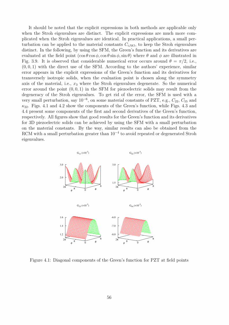
It should be noted that the explicit expressions in both methods are applicable onlywhen the Stroh eigenvalues are distinct. The explicit expressions are much more com-plicated when the Stroh eigenvalues are identical. In practical applications, a small per-turbation can be applied to the material constants CiJKl, to keep the Stroh eigenvaluesdistinct. In the following, by using the SFM, the Green’s function and its derivatives areevaluated at the field point (cos θ cosφ, cos θ sinφ, sin θ) where θ and φ are illustrated inFig. 3.9. It is observed that considerable numerical error occurs around θ = π/2, i.e.,(0, 0, 1) with the direct use of the SFM. According to the authors’ experience, similarerror appears in the explicit expressions of the Green’s function and its derivatives fortransversely isotropic solids, when the evaluation point is chosen along the symmetryaxis of the material, i.e., x3 where the Stroh eigenvalues degenerate. So the numericalerror around the point (0, 0, 1) in the SFM for piezoelectric solids may result from thedegeneracy of the Stroh eigenvalues. To get rid of the error, the SFM is used with avery small perturbation, say 10−6, on some material constants of PZT, e.g., C22, C55 andκ22. Figs. 4.1 and 4.2 show the components of the Green’s function, while Figs. 4.3 and4.4 present some components of the first and second derivatives of the Green’s function,respectively. All figures show that good results for the Green’s function and its derivativesfor 3D piezoelectric solids can be achieved by using the SFM with a small perturbationon the material constants. By the way, similar results can also be obtained from theRCM with a small perturbation greater than 10−4 to avoid repeated or degenerated Stroheigenvalues.

G11 (×10-3

)

0

π

θπ2π

φ

2.0

3.0

G22 (×10-3

)

0

π

θπ2π

φ

1.5

3.0

G33 (×10-3

)

0

π

θπ2π

φ

1.2

1.4

1.6

G44 (×10-3

)

0

π

θπ2π

φ

-8.0

-7.0

-6.0

Figure 4.1: Diagonal components of the Green’s function for PZT at field points

56

G12 (×10-4

)

0

π

θπ2π

φ

-4.0

0.0

4.0

G13 (×10-4

)

0

π

θπ2π

φ

-3.0

0.0

3.0

G14 (×10-4

)

0

π

θπ2π

φ

-4.0

0.0

4.0

G23 (×10-4

)

0

π

θπ2π

φ

-3.0

0.0

3.0

G24 (×10-4

)

0

π

θπ2π

φ

-4.0

0.0

4.0

G34 (×10-3

)

0

π

θπ2π

φ

2.5

3.0

Figure 4.2: Non-diagonal components of the Green’s function for PZT at field points

57

G11,1 (×10-3

)

0

π

θπ2π

φ

-2.0

0.0

2.0

G14,1 (×10-4

)

0

π

θπ2π

φ

-6.0

0.0

6.0

G11,2 (×10-3

)

0

π

θπ2π

φ

-2.0

0.0

2.0

G14,2 (×10-4

)

0

π

θπ2π

φ

-6.0

0.0

6.0

G11,3 (×10-3

)

0

π

θπ2π

φ

-2.0

-1.0

0.0

G14,3 (×10-3

)

0

π

θπ2π

φ

-1.0

0.0

1.0

Figure 4.3: Some components of the first derivative of the Green’s function for PZT atfield points

58

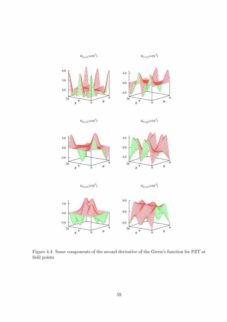
G11,11 (×10-3

)

0

π

θπ2π

φ

0.0

3.0

6.0

G11,12 (×10-3

)

0

π

θπ2π

φ

-4.0

0.0

4.0

G11,13 (×10-3

)

0

π

θπ2π

φ

-4.0

0.0

4.0

G11,22 (×10-3

)

0

π

θπ2π

φ

-4.0

0.0

4.0

G11,23 (×10-3

)

0

π

θπ2π

φ

-3.0

0.0

3.0

G11,33 (×10-3

)

0

π

θπ2π

φ

-6.0

0.0

6.0

Figure 4.4: Some components of the second derivative of the Green’s function for PZT atfield points

59

4.6 Concluding remarksIn this chapter, two accurate methods are presented for computing the Green’s functionand its first and second derivatives for three-dimensional anisotropic piezoelectric solids.The derivatives of the generalized displacement Green’s function are needed for comput-ing the generalized stress and higher-order stress Green’s functions, which are required bythe displacement-based and stress-based BEM or by the integral representation formulaefor calculating the generalized displacement and stress at internal points in the analyzeddomain. In the first method, the Stroh formalism is applied to derive explicit expressionsfor the Green’s function as well as its first and second derivatives as a linear combinationof the Stroh eigenvectors. The coefficients are expressed in terms of the eigenvalues andthe eigenvectors. In the second method, the Cauchy residue theorem is applied to theinfinite or improper line integrals arising in the Green’s function and its derivatives, whichcan be evaluated analytically. Both methods work well under the assumption that theStroh eigenvalues are distinct. The obtained new expressions by the two methods areimplemented into a FORTRAN code. Good accuracy of both methods is verified by theresults from the analytical solutions. If a similar accuracy is required, the expressions ob-tained by the Stroh formalism method are much more efficient than those by the residuecalculus method. Although the new explicit expressions in both methods are only appli-cable when the Stroh eigenvalues are distinct, a general evaluation of the Green’s functionand its derivatives can be performed by using these expressions with a small perturbationin the material constants to avoid repeated or identical eigenvalues.

60

Chapter 5

Green’s function in linearmagnetoelectroelasticity

5.1 Problem statementMagnetoelectroelastic solids and/or multiferroic materials have magneto-electro-mechanicalenergy conversion capacities. Due to the potential applications in the technologies ofsmart and adaptive materials and structures such as magnetic/electric transducers, ac-tuators and sensors, the magnetoelectroelastic solids have drawn increasing interest ofthe scientists and engineers. The natural single-phase multiferroic materials have veryweak magnetoelectric coupling at room temperature, while the magnetoelectric compos-ites constituting of piezoelectric and piezomagnetic material phases, reported for exampleby van Suchtelen (1972), may have a strong magnetoelectric coupling even at room tem-perature (Eerenstein et al., 2006; Srinivasan, 2010).

Although there is no magnetoelectric coupling in either piezoelectric materials or piezo-magnetic materials, the magnetoelectric composites have a magnetoelectric coupling dueto the interaction between the electromechanical and magnetomechanical behaviors of theconstituent materials. Many investigations can be found in literature on the theoreticalmodeling of magnetoelectric composites. Alshits et al. (1992) investigated the existenceof the surface wave in semi-infinite anisotropic magnetoelectroelastic solids, Benveniste(1995), Huang and Kuo (1997) and Li and Dunn (1998) analyzed the inclusion and inho-mogeneity problems of the magnetoelectric composites by treating both the piezoelectricand the piezomagnetic materials as single-phase magnetoelectroelastic materials. Theseprevious works may be considered as some of the pioneer works on the magnetoelectroe-lastic materials after which numerous theoretical models have been proposed.

The Green’s function in the magnetoelectroelastic materials has already been investi-gated by some researchers. For the transversely isotropic magnetoelectroelastic materials,the Green’s function could be obtained analytically by using the potential theory. Wangand Shen (2002) derived the fundamental solution for the dislocation and the Green’sfunction in a half-space magnetoelectroelastic solid. Soh et al. (2003) and Ding and Jiang(2003) derived the Green’s function in a full-space magnetoelectroelastic solid and thelater authors implemented the Green’s function in the BEM. For generally anisotropicmaterials, the Green’s function can be represented explicitly in terms of the Stroh eigen-values or Stroh eigenvectors. Chung and Ting (1995) presented the two-dimensional (2D)Green’s function for anisotropic magnetoelectroelastic materials with an elliptic hole or

61

rigid inclusion by the Stroh formalism in magnetoelectroelasticity. Liu et al. (2001) pre-sented the 2D Green’s function for anisotropic magnetoelectroelastic solids with an el-liptical cavity or a crack based on the Stroh formalism combined with the technique ofconformal mapping and the Laurent series expansion. Further, Pan (2002) derived thethree-dimensional (3D) Green’s functions in anisotropic magnetoelectroelastic full-space,half-space, and bimaterials based on the Stroh formalism. Qin (2004) derived the Green’sfunctions with an arbitrarily oriented half-plane or bimaterial interface. Buroni and Saez(2010) presented the 3D anisotropic magnetoelectroelastic Green’s function and its firstand second derivatives in terms of the Stroh eigenvalues by the Cauchy residue calcu-lus applied to the line integrals. More details on the anisotropic and multifield coupledGreen’s function can be found in the textbooks by Qin (2010) and Pan and Chen (2015).

In this Chapter, the explicit expression for the 3D generally anisotropic magnetoelec-troelastic Green’s function is derived by using the Stroh formalism associated with anoblique plane in the 3D full-space. Since the derivatives of the Green’s function are alsoessential issues in BEM as well as many other applications, the explicit derivatives ofthe Green’s function are also derived based on the Stroh eigen-relation on the obliqueplane and the orthonormal or orthogonality relation for the Green’s function. The maindifference between the novel expressions and those proposed by Buroni and Saez (2010)are that in the present paper, we utilize the Stroh formalism while the later used Cauchyresidue calculus to evaluate the Green’s function and its derivatives. Although the numer-ical results of the second derivative of the Green’s function was not presented, Buroni andSaez (2010) pointed out that it could be obtained by applying the Cauchy residue calculusto the line integral. In this work, not only the explicit expressions for the first derivativebut also for the second derivative of the Green’s function as well as the correspondingnumerical results are presented. Besides, Xie et al. (2015b) demonstrated that the Strohformalism method may have advantages compared to the residue calculus method for thenumerical calculations of the Green’s function and its derivatives. The newly proposedexpressions for 3D generally anisotropic magnetoelectroelastic solids are verified by thecomparison of the present numerical results and those evaluated by the analytical solu-tions derived by Ding and Jiang (2003) for transversely isotropic magnetoelectroelasticsolids at a particular point. The CPU time for the calculation of the Green’s function andits derivatives is also given. In addition, for degenerate and nearly degenerate cases theGreen’s function and its derivatives at arbitrary field points by the present novel explicitexpressions with a small perturbation on some material coefficients are also computedand discussed for practical interest.

The contribution in this chapter has been published in:

• L. Xie, C. Zhang, C. Hwu, E. Pan, On novel explicit expressions of Green’s func-tion and its derivatives for magnetoelectroelastic materials. European Journal ofMechanics – A/Solids. submitted.

5.2 Stroh formalism methodIn Chapters 3 and 4, it is demonstrated that compared to the residue calculus method, theStroh formalism may have higher accuracy and efficiency in the numerical calculation ofthe Green’s function and its derivatives. So in this section, we extend the Stroh formalism

62

method proposed in Chapter 3 and 4 to derive the Green’s function and its first and secondderivatives for linear generally anisotropic magnetoelectroelastic materials.

5.2.1 Representation of the Green’s functionIn linear elastic and piezoelectric solids, the Green’s function can be constructed fromthe solutions of the Stroh eigenvalue problem. Similarly, in linear magnetoelectroelasticsolids, the 3D Green’s function can also be constructed from the solutions of the Stroheigenvalue problem in magnetoelectroelasticity. The Stroh eigenvalue problem in thelinear magnetoelectroelastic solids in terms of the fundamental magnetoelectroelasticitymatrix N is given by

Nξ = pξ, (5.1)where

N =(

N1 N2N3 NT

1

), (5.2a)

N1 = −T−1RT , N2 = T−1 = NT2 , N3 = RT−1RT −Q,

in whichQIJ = ckIJlnknl, RIJ = ckIJlnkml, TIJ = ckIJlmkml. (5.2b)

Here, n and m are two mutually orthogonal unit vectors on the oblique plane perpendic-ular to x. Since the fundamental magnetoelectroelasticity matrix N is a non-symmetric10×10 matrix, the vector ξ is a 10-dimensional right eigenvector of the matrix N. If theright eigenvector ξ is denoted as

ξ =ab

, (5.3)

where a and b are two 5-dimensional vectors, then as proved by Ting (1996) in linearelastic solids, the corresponding left eigenvector η of the matrix N is determined by

η =ba

. (5.4)

Similar to the elastic and piezoelectric cases, the eigenvalues of the matrix N shouldbe 5 pairs of complex conjugates. Among the eigenvalues, we choose Im(pK) > 0, K =1, 2, . . . , 5, which are known as Stroh eigenvalues, and pK+5 = pK . Further, we assume thatthe Stroh eigenvalues pK (K = 1, 2, . . . , 5) are distinct, which ensures that the eigenvectorsassociated with the different Stroh eigenvalues are independent of each other.

By definingA = [a1,a2,a3,a4,a5] , B = [b1, b2, b3, b4, b5] , (5.5)

and with the following orthonormal relation between the left and the right eigenvectors

ηTαξβ = δαβ, α, β = 1, 2, . . . , 10, (5.6)

where δαβ is the Kronecker delta, the Green’s function can be expressed as

G(x) = 14πrH(x), H = 2iAAT , (5.7)

in which r = |x|, x is the unit vector of x, and H is one of the three Barnett-Lothematrices in linear magnetoelectroelasticity.

63

5.2.2 First derivative of the Green’s functionDifferentiation of Eq. (5.7) with respect to xi yields the first derivative of the Green’sfunction as

G,i(x) = 14πr2

(−xir

H + rH,i

), (5.8a)

whereH,i = 2i

(A,iAT +

[A,iAT

]T). (5.8b)

The columns of the matrix A are parts of the eigenvectors satisfying Eq. (5.6). So inorder to calculate the first derivative of the Green’s function, we need to firstly calculatethe first derivatives of the eigenvectors satisfying Eqs. (5.1) and (5.6). In the following,with the distinctness assumption of the eigenvalues, the derivation of the first derivativesof the eigenvectors is presented.

Differentiating Eq. (5.1), associated with the eigenvalue pα and the corresponding righteigenvector ξα, with respect to xi leads to


Note here that the repeated Greek indices do not imply summation. As the 10-dimensionaleigenvectors associated with distinct eigenvalues are independent of each other and thederivative of an eigenvector is still a vector in the 10-dimensional space, the first derivativeof the right eigenvector ξα,i is a linear combination of the 10 independent eigenvectors,i.e.,

ξα,i =10∑β=1

c(i)αβξβ, (5.10a)

andηα,i =

10∑β=1

c(i)αβηβ, (5.10b)

where c(i)αβ are constants to be determined. Substitution of Eq. (5.10a) into Eq. (5.9)

followed by the pre-multiplication by ηTβ yields

c(i)αβ(pβ − pα) = −ηTβ (N,i − pα,iI)ξα, (5.11)

which results from the use of Eqs. (5.1) and (5.6). When β = α, the derivative of theeigenvalue pα is obtained by


If β 6= α, the coefficients c(i)αβ are given by

c(i)αβ =


. (5.13)


c(i)αβ + c

(i)βα = 0. (5.14)


64

Although similar expressions as Eqs. (5.13) and (5.15) were derived by Malen (1971),Lavagnino (1995) and Pan and Chen (2015), the present expression may be preferred sinceit is in the Cartesian coordinate system rather than in the spherical coordinate system. Inthe conventional methods, in order to get the expressions of the derivatives of the Green’sfunction in the Cartesian coordinate system, the corresponding expressions in the sphericalcoordinate system have to be tranformed into the desired ones in the Cartesian coordinatesystem. While in the present method, the vectors n andm are expressed directly in termsof the Cartesian coordinates and consequently also the expressions of the derivatives ofthe Green’s function.

So far, since all coefficients c(i)αβ are determined, the first derivatives of the eigenvectors

can be determined explicitly in terms of the eigenvalues and the eigenvectors. The explicitexpression of the derivative of the fundamental magnetoelectroelasticity matrix N,i ispresented in Appendix B. Thereafter the first derivatives of the eigenvectors can be usedto construct the matrices A,i as well as the first derivative of the Green’s function.

5.2.3 Second derivative of the Green’s functionDifferentiating Eq. (5.8) with respect to xj yields the second derivative of the Green’sfunction

G,ij(x) = 14πr3

[(3xixjr2 − δij


], (5.16a)

whereH,ij = 2i

[A,ijAT + A,iAT

,j +(A,ijAT + A,iAT

,j

)T ]. (5.16b)

In order to calculate the second derivative of the Green’s function, we need to know thesecond derivative of the matrix A which is constructed from the second derivatives of theeigenvectors ξα,ij (α = 1, 2, . . . , 5). Since ξα,ij is a 10-dimensional vector, it is a linearcombination of the 10 independent eigenvectors, i.e.,

ξα,ij =10∑β=1

d(ij)αβ ξβ, (5.17)

where d(ij)αβ are constants to be determined. Following the similar procedure to determine

c(i)αβ, the expressions of d(ij)

αβ can be derived by differentiating Eqs. (5.1) and (5.6) withrespect to xi and further to xj. They are

d(ij)αα = −(ηTα,iξα,j + ηTα,jξα,i)/2,

d(ij)αβ =


, β 6= α. (5.18)

The explicit expressions of N,ij can be found in Appendix B.

5.3 Numerical examples and discussionsThe verification of the present novel expressions of the Green’s function and its derivativesis presented in the following for a virtual transversely isotropic magnetoelectroelastic

65

solid used by Pan (2002). The nonzero coefficients of the virtual solid in the contractednotations are given by

c11 = 166, c12 = 77, c13 = 78, c33 = 162, c44 = 43, c66 = 44.5,e31 = −4.4, e33 = 18.6, e15 = 11.6, κ11 = 11.2, κ33 = 12.6, (5.19)h31 = 580.3, h33 = 699.7, h15 = 550, µ11 = 5, µ33 = 10.

The units of the coefficients cij, eij, κij, hij and µij are 109N/m2, C/m2, 10−9C/(Vm),N/(Am) and 10−6Ns2/C2, respectively.

In order to validate the derived formulae, they are implemented into FORTRAN code.The Stroh eigen-relation Eq. (5.1) is solved by the subroutine ZGEEV in LAPACK li-brary (Anderson et al., 1999). Note the eigenvectors should be normalized by Eqs. (3.36)and (3.37) to be the right ones for the Green’s function and its derivatives. The numeri-cal results are compared with those of the analytical solutions derived by Ding and Jiang(2003) which are obtained by the software MATHEMATICA where the derivatives of theGreen’s function are evaluated by algebraic algorithm. We point out here that in ourGreen’s function solutions, the only numerical technique involved is the solution of theStroh eigenequation. However, by controlling the accuracy in the Stroh eigenvalues andeigenvectors, one can obtain the Green’s function as accurate as one wishes. For exam-ple, Tables 5.1-5.3 are the numerical results from the present method, which are exactlythe same as those of the analytical solutions in Ref.(Ding and Jiang, 2003) even after 10digits. The high accuracy of the numerical results demonstrate that the present novel for-mulae are correct and accurate for generally anisotropic magnetoelectroelastic materials.It should be noted here that the remaining components of the Green’s function and itsderivatives, which are not listed in Tables 1-3, can be obtained by using the symmetryproperty of the Green’s function.

G11 314.16063654 G12 22.361037823 G24 71.012378811G22 347.70219328 G13 42.153781088 G25 -3.3834594255G33 97.861922990 G14 35.506189405 G34 82.045333135G44 -1788.9486757 G15 -1.6917297128 G35 33.169143465G55 -4.8033844483 G23 84.307562176 G45 38.107859915

Table 5.1: Numerical results of the Green’s function Gij(×10−6) at the point (1, 2, 3)m.

The efficiency of the present novel expressions is revealed by the CPU time for thecalculation of the Green’s function and its derivatives on the high performance computercluster of the University of Siegen, Germany. The second column of Table 5.4 is theCPU time for the calculation of the Green’s function. The third column is the additionalCPU time for the calculation of the first derivative of the Green’s function. And the lastcolumn is the additional CPU time for the calculation of the second derivative of theGreen’s function.

The accuracy of the present novel formulae is confirmed by the numerical example eval-uated at the point (1, 2, 3)m for the transversely isotropic magnetoelectroelastic material.However, strictly speaking, the formulae are inapplicable when some Stroh eigenvaluesare identical (degenerate cases), and in the numerical evaluation, significant errors mayarise when some Stroh eigenvalues are very close to each other (nearly degenerate cases).

66

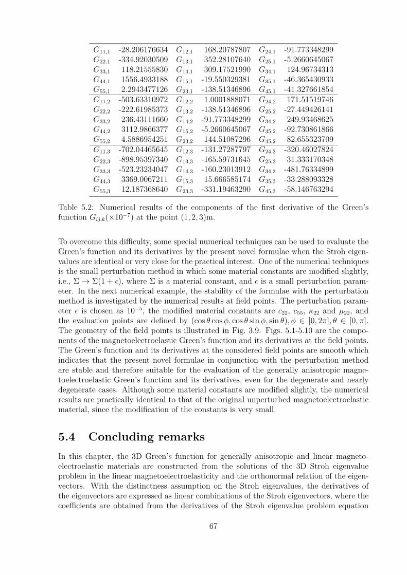
G11,1 -28.206176634 G12,1 168.20787807 G24,1 -91.773348299G22,1 -334.92030509 G13,1 352.28107640 G25,1 -5.2660645067G33,1 118.21555830 G14,1 309.17521990 G34,1 124.96734313G44,1 1556.4933188 G15,1 -19.550329381 G35,1 -46.365430933G55,1 2.2943477126 G23,1 -138.51346896 G45,1 -41.327661854G11,2 -503.63310972 G12,2 1.0001888071 G24,2 171.51519746G22,2 -222.61985373 G13,2 -138.51346896 G25,2 -27.449426141G33,2 236.43111660 G14,2 -91.773348299 G34,2 249.93468625G44,2 3112.9866377 G15,2 -5.2660645067 G35,2 -92.730861866G55,2 4.5886954251 G23,2 144.51087296 G45,2 -82.655323709G11,3 -702.04465645 G12,3 -131.27287797 G24,3 -320.46027824G22,3 -898.95397340 G13,3 -165.59731645 G25,3 31.333170348G33,3 -523.23234047 G14,3 -160.23013912 G34,3 -481.76334899G44,3 3369.0067211 G15,3 15.666585174 G35,3 -33.288093328G55,3 12.187368640 G23,3 -331.19463290 G45,3 -58.146763294

Table 5.2: Numerical results of the components of the first derivative of the Green’sfunction Gij,k(×10−7) at the point (1, 2, 3)m.

To overcome this difficulty, some special numerical techniques can be used to evaluate theGreen’s function and its derivatives by the present novel formulae when the Stroh eigen-values are identical or very close for the practical interest. One of the numerical techniquesis the small perturbation method in which some material constants are modified slightly,i.e., Σ→ Σ(1 + ε), where Σ is a material constant, and ε is a small perturbation param-eter. In the next numerical example, the stability of the formulae with the perturbationmethod is investigated by the numerical results at field points. The perturbation param-eter ε is chosen as 10−5, the modified material constants are c22, c55, κ22 and µ22, andthe evaluation points are defined by (cos θ cosφ, cos θ sinφ, sin θ), φ ∈ [0, 2π], θ ∈ [0, π].The geometry of the field points is illustrated in Fig. 3.9. Figs. 5.1-5.10 are the compo-nents of the magnetoelectroelastic Green’s function and its derivatives at the field points.The Green’s function and its derivatives at the considered field points are smooth whichindicates that the present novel formulae in conjunction with the perturbation methodare stable and therefore suitable for the evaluation of the generally anisotropic magne-toelectroelastic Green’s function and its derivatives, even for the degenerate and nearlydegenerate cases. Although some material constants are modified slightly, the numericalresults are practically identical to that of the original unperturbed magnetoelectroelasticmaterial, since the modification of the constants is very small.

5.4 Concluding remarksIn this chapter, the 3D Green’s function for generally anisotropic and linear magneto-electroelastic materials are constructed from the solutions of the 3D Stroh eigenvalueproblem in the linear magnetoelectroelasticity and the orthonormal relation of the eigen-vectors. With the distinctness assumption on the Stroh eigenvalues, the derivatives ofthe eigenvectors are expressed as linear combinations of the Stroh eigenvectors, where thecoefficients are obtained from the derivatives of the Stroh eigenvalue problem equation

67

G11,11 -84.923711750 G12,11 -143.43833544 G24,11 -93.425960108G22,11 -246.67909237 G13,11 -199.22866956 G25,11 1.2064201003G33,11 -5.2122015353 G14,11 -138.48632835 G34,11 18.552929152G44,11 1136.3796110 G15,11 -4.6628544565 G35,11 -32.565220675G55,11 2.7269371665 G23,11 -121.43040120 G45,11 -31.699237588G11,22 -35.466694098 G12,22 -75.130840388 G24,22 -281.93049213G22,22 -201.56507722 G13,22 -35.090598953 G25,22 10.091744908G33,22 -375.49548105 G14,22 -49.191897767 G34,22 -300.69031277G44,22 -123.96151242 G15,22 10.311936961 G35,22 8.8354100986G55,22 4.0247055283 G23,22 -347.20813583 G45,22 -2.8139647883G11,33 211.55693097 G12,33 84.382350809 G24,33 111.92891588G22,33 338.13045718 G13,33 35.419945056 G25,33 -25.056412010G33,33 202.99260238 G14,33 55.964457942 G34,33 233.85887683G44,33 -818.83147104 G15,33 -12.528206005 G35,33 -16.749738620G55,33 -3.0993622005 G23,33 70.839890112 G45,33 -3.3693045985G11,12 -2.6300699248 G12,12 18.837268767 G24,12 -49.191897767G22,12 65.677425129 G13,12 -121.43040120 G25,12 10.311936961G33,12 -246.85551967 G14,12 -93.425960108 G34,12 -212.82882795G44,12 -840.22741562 G15,12 1.2064201003 G35,12 27.600420516G55,12 0.86517890784 G23,12 -35.090598953 G45,12 19.256848533G11,13 48.865401622 G12,13 -76.883986080 G24,13 125.11881741G22,13 261.72161743 G13,13 -87.490893614 G25,13 -3.7660550027G33,13 87.497374760 G14,13 -97.670730413 G34,13 52.390013497G44,13 -856.30380581 G15,13 13.783557673 G35,13 23.365080503G55,13 -3.0153301358 G23,13 156.21284568 G45,13 25.280288077G11,23 360.27655919 G12,23 43.141344798 G24,23 90.007495707G22,23 260.89747892 G13,23 156.21284568 G25,23 8.1344751687G33,23 174.99474952 G14,23 125.11881741 G34,23 104.78002699G44,23 -1712.6076116 G15,23 -3.7660550027 G35,23 46.730161006G55,23 -6.0306602716 G23,23 146.82837490 G45,23 50.560576154

Table 5.3: Numerical results of the components of the second derivative of the Green’sfunction Gij,kl(×10−7) at the point (1, 2, 3)m.

GIJ GIJ,k GIJ,kl

CPU Time (10−4s) 1.40805340 2.18008423 7.67242527

Table 5.4: The CPU time for the calculation of the Green’s function and its derivativesby the novel explicit expressions

68

G11

×10-3

0

π

θπ2π

φ

1.0

1.5

G22

×10-3

0

π

θπ2π

φ

1.0

1.5

G33

×10-4

0

π

θπ2π

φ

1.0

4.0

G44

×10-3

0

π

θπ2π

φ

-7.0

-6.5

G55

×10-5

0

π

θπ2π

φ

-2.0

-1.5

G12

×10-4

0

π

θπ2π

φ

-3.0

3.0

G13

×10-4

0

π

θπ2π

φ

-3.0

3.0

G14

×10-4

0

π

θπ2π

φ

-3.0

3.0

G15

×10-5

0

π

θπ2π

φ

-3.0

3.0

G23

×10-4

0

π

θπ2π

φ

-3.0

3.0

G24

×10-4

0

π

θπ2π

φ

-3.0

3.0

G25

×10-5

0

π

θπ2π

φ

-3.0

3.0

G34

×10-4

0

π

θπ2π

φ

1.0

4.0

G35

×10-4

0

π

θπ2π

φ

1.0

1.4

G45

×10-4

0

π

θπ2π

φ

1.3

1.5

Figure 5.1: Variation of the Green’s function GIJ on upper half unit sphere with thesource point at the origin.

69

G11,1

×10-3

0

π

θπ2π

φ

-1.0

1.0

G22,1

×10-3

0

π

θπ2π

φ

-1.0

1.0

G33,1

×10-4

0

π

θπ2π

φ

-4.0

4.0

G44,1

×10-3

0

π

θπ2π

φ

-4.0

4.0

G55,1

×10-5

0

π

θπ2π

φ

-1.0

1.0

G12,1

×10-4

0

π

θπ2π

φ

-4.0

4.0

G13,1

×10-4

0

π

θπ2π

φ

-3.0

3.0

G14,1

×10-4

0

π

θπ2π

φ

-3.0

3.0

G15,1

×10-5

0

π

θπ2π

φ

-2.0

2.0

G23,1

×10-4

0

π

θπ2π

φ

-2.0

2.0

G24,1

×10-4

0

π

θπ2π

φ

-2.0

2.0

G25,1

×10-5

0

π

θπ2π

φ

-2.0

2.0

G34,1

×10-4

0

π

θπ2π

φ

-3.0

3.0

G35,1

×10-4

0

π

θπ2π

φ

-1.0

1.0

G45,1

×10-4

0

π

θπ2π

φ

-1.0

1.0

Figure 5.2: Variation of the first derivative of the Green’s function GIJ,1 on upper halfunit sphere with the source point at the origin.

70

G11,2

×10-3

0

π

θπ2π

φ

-1.0

1.0

G22,2

×10-3

0

π

θπ2π

φ

-1.0

1.0

G33,2

×10-4

0

π

θπ2π

φ

-4.0

4.0

G44,2

×10-3

0

π

θπ2π

φ

-4.0

4.0

G55,2

×10-5

0

π

θπ2π

φ

-1.0

1.0

G12,2

×10-4

0

π

θπ2π

φ

-4.0

4.0

G13,2

×10-4

0

π

θπ2π

φ

-3.0

3.0

G14,2

×10-4

0

π

θπ2π

φ

-3.0

3.0

G15,2

×10-5

0

π

θπ2π

φ

-2.0

2.0

G23,2

×10-4

0

π

θπ2π

φ

-2.0

4.0

G24,2

×10-4

0

π

θπ2π

φ

-2.0

4.0

G25,2

×10-5

0

π

θπ2π

φ

-2.0

2.0

G34,2

×10-4

0

π

θπ2π

φ

-3.0

3.0

G35,2

×10-4

0

π

θπ2π

φ

-1.0

1.0

G45,2

×10-4

0

π

θπ2π

φ

-1.0

1.0


71

G11,3

×10-4

0

π

θπ2π

φ

-8.0

-2.0

G22,3

×10-4

0

π

θπ2π

φ

-8.0

-2.0

G33,3

×10-4

0

π

θπ2π

φ

-5.0

-1.0

G44,3

×10-3

0

π

θπ2π

φ

2.0

6.0

G55,3

×10-5

0

π

θπ2π

φ

0

1.4

G12,3

×10-4

0

π

θπ2π

φ

-4.0

4.0

G13,3

×10-4

0

π

θπ2π

φ

-6.0

6.0

G14,3

×10-4

0

π

θπ2π

φ

-6.0

6.0

G15,3

×10-5

0

π

θπ2π

φ

-8.0

8.0

G23,3

×10-4

0

π

θπ2π

φ

-6.0

6.0

G24,3

×10-4

0

π

θπ2π

φ

-6.0

6.0

G25,3

×10-5

0

π

θπ2π

φ

-6.0

6.0

G34,3

×10-4

0

π

θπ2π

φ

-4.0

-1.0

G35,3

×10-5

0

π

θπ2π

φ

-9.0

-4.0

G45,3

×10-4

0

π

θπ2π

φ

-1.0

-0.5


72

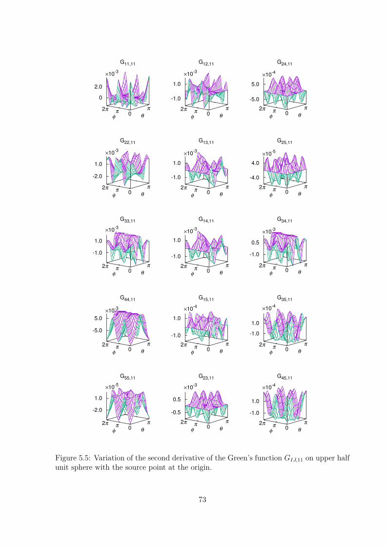
G11,11

×10-3

0

π

θπ2π

φ

0

2.0

G22,11

×10-3

0

π

θπ2π

φ

-2.0

1.0

G33,11

×10-3

0

π

θπ2π

φ

-1.0

1.0

G44,11

×10-3

0

π

θπ2π

φ

-5.0

5.0

G55,11

×10-5

0

π

θπ2π

φ

-2.0

1.0

G12,11

×10-3

0

π

θπ2π

φ

-1.0

1.0

G13,11

×10-3

0

π

θπ2π

φ

-1.0

1.0

G14,11

×10-3

0

π

θπ2π

φ

-1.0

1.0

G15,11

×10-4

0

π

θπ2π

φ

-1.0

1.0

G23,11

×10-3

0

π

θπ2π

φ

-0.5

0.5

G24,11

×10-4

0

π

θπ2π

φ

-5.0

5.0

G25,11

×10-5

0

π

θπ2π

φ

-4.0

4.0

G34,11

×10-3

0

π

θπ2π

φ

-1.0

0.5

G35,11

×10-4

0

π

θπ2π

φ

-1.0

1.0

G45,11

×10-4

0

π

θπ2π

φ

-1.0

1.0

Figure 5.5: Variation of the second derivative of the Green’s function GIJ,11 on upper halfunit sphere with the source point at the origin.

73

G11,22

×10-3

0

π

θπ2π

φ

-1.5

1.5

G22,22

×10-3

0

π

θπ2π

φ

0

2.0

G33,22

×10-3

0

π

θπ2π

φ

-1.0

1.0

G44,22

×10-3

0

π

θπ2π

φ

-7.0

3.0

G55,22

×10-5

0

π

θπ2π

φ

-2.0

1.0

G12,22

×10-3

0

π

θπ2π

φ

-1.0

1.0

G13,22

×10-4

0

π

θπ2π

φ

-5.0

5.0

G14,22

×10-4

0

π

θπ2π

φ

-5.0

5.0

G15,22

×10-5

0

π

θπ2π

φ

-4.0

4.0

G23,22

×10-4

0

π

θπ2π

φ

-9.0

9.0

G24,22

×10-3

0

π

θπ2π

φ

-0.6

0.8

G25,22

×10-5

0

π

θπ2π

φ

-9.0

9.0

G34,22

×10-3

0

π

θπ2π

φ

-1.0

0.5

G35,22

×10-4

0

π

θπ2π

φ

-1.0

1.0

G45,22

×10-4

0

π

θπ2π

φ

-1.0

1.0


74

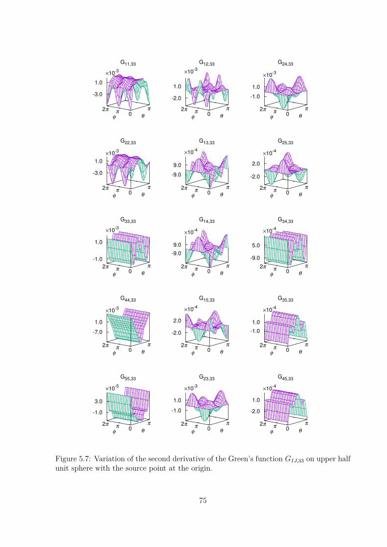
G11,33

×10-3

0

π

θπ2π

φ

-3.0

1.0

G22,33

×10-3

0

π

θπ2π

φ

-3.0

1.0

G33,33

×10-3

0

π

θπ2π

φ

-1.0

1.0

G44,33

×10-3

0

π

θπ2π

φ

-7.0

1.0

G55,33

×10-5

0

π

θπ2π

φ

-1.0

3.0

G12,33

×10-3

0

π

θπ2π

φ

-2.0

1.0

G13,33

×10-4

0

π

θπ2π

φ

-9.0

9.0

G14,33

×10-4

0

π

θπ2π

φ

-9.0

9.0

G15,33

×10-4

0

π

θπ2π

φ

-2.0

2.0

G23,33

×10-3

0

π

θπ2π

φ

-1.0

1.0

G24,33

×10-3

0

π

θπ2π

φ

-1.0

1.0

G25,33

×10-4

0

π

θπ2π

φ

-2.0

2.0

G34,33

×10-4

0

π

θπ2π

φ

-9.0

5.0

G35,33

×10-4

0

π

θπ2π

φ

-1.0

1.0

G45,33

×10-4

0

π

θπ2π

φ

-2.0

1.0


75

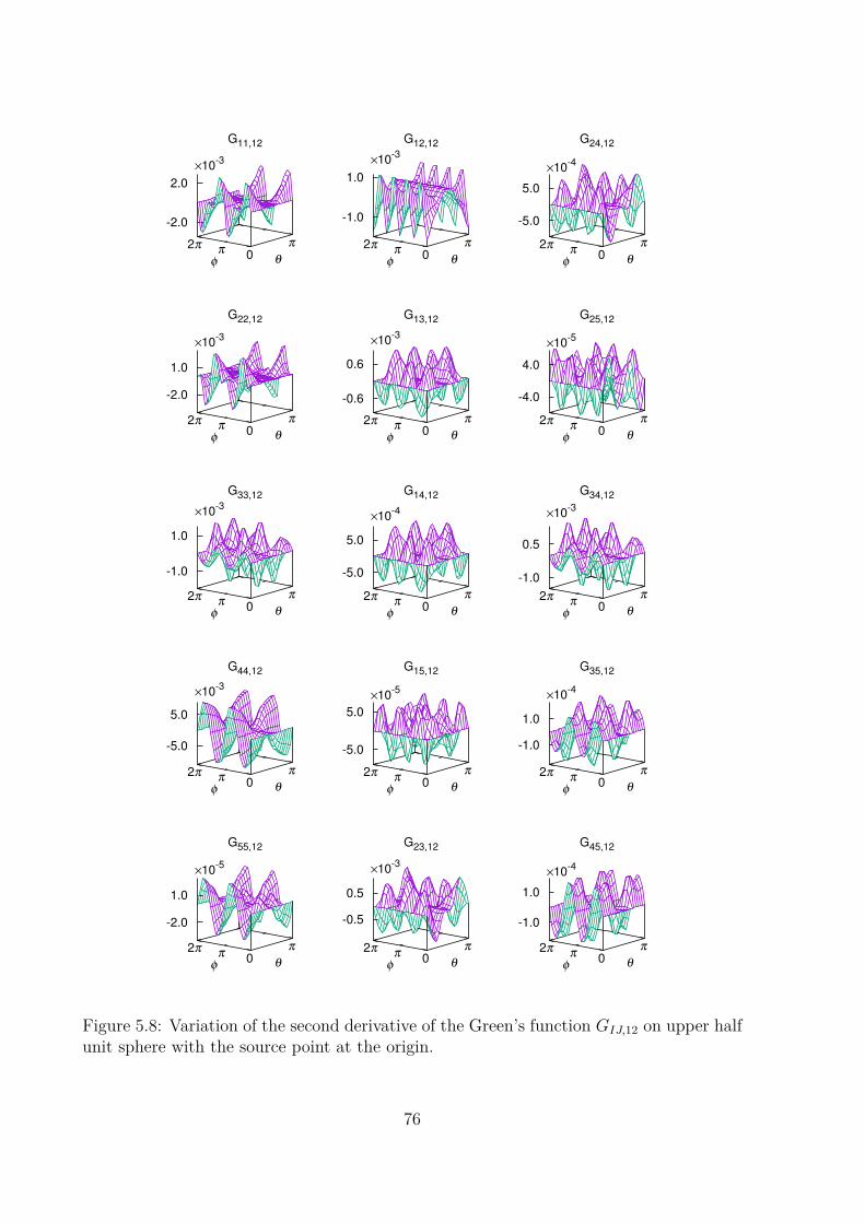
G11,12

×10-3

0

π

θπ2π

φ

-2.0

2.0

G22,12

×10-3

0

π

θπ2π

φ

-2.0

1.0

G33,12

×10-3

0

π

θπ2π

φ

-1.0

1.0

G44,12

×10-3

0

π

θπ2π

φ

-5.0

5.0

G55,12

×10-5

0

π

θπ2π

φ

-2.0

1.0

G12,12

×10-3

0

π

θπ2π

φ

-1.0

1.0

G13,12

×10-3

0

π

θπ2π

φ

-0.6

0.6

G14,12

×10-4

0

π

θπ2π

φ

-5.0

5.0

G15,12

×10-5

0

π

θπ2π

φ

-5.0

5.0

G23,12

×10-3

0

π

θπ2π

φ

-0.5

0.5

G24,12

×10-4

0

π

θπ2π

φ

-5.0

5.0

G25,12

×10-5

0

π

θπ2π

φ

-4.0

4.0

G34,12

×10-3

0

π

θπ2π

φ

-1.0

0.5

G35,12

×10-4

0

π

θπ2π

φ

-1.0

1.0

G45,12

×10-4

0

π

θπ2π

φ

-1.0

1.0


76

G11,13

×10-3

0

π

θπ2π

φ

-1.0

1.0

G22,13

×10-3

0

π

θπ2π

φ

-1.0

1.0

G33,13

×10-3

0

π

θπ2π

φ

-1.0

1.0

G44,13

×10-3

0

π

θπ2π

φ

-5.0

5.0

G55,13

×10-5

0

π

θπ2π

φ

-1.0

2.0

G12,13

×10-4

0

π

θπ2π

φ

-5.0

5.0

G13,13

×10-3

0

π

θπ2π

φ

-1.0

1.0

G14,13

×10-3

0

π

θπ2π

φ

-1.2

0.6

G15,13

×10-4

0

π

θπ2π

φ

-0.5

1.5

G23,13

×10-3

0

π

θπ2π

φ

-0.5

0.5

G24,13

×10-3

0

π

θπ2π

φ

-0.5

0.5

G25,13

×10-4

0

π

θπ2π

φ

-1.0

1.0

G34,13

×10-4

0

π

θπ2π

φ

-8.0

6.0

G35,13

×10-4

0

π

θπ2π

φ

-1.5

2.0

G45,13

×10-4

0

π

θπ2π

φ

-1.0

1.0


77

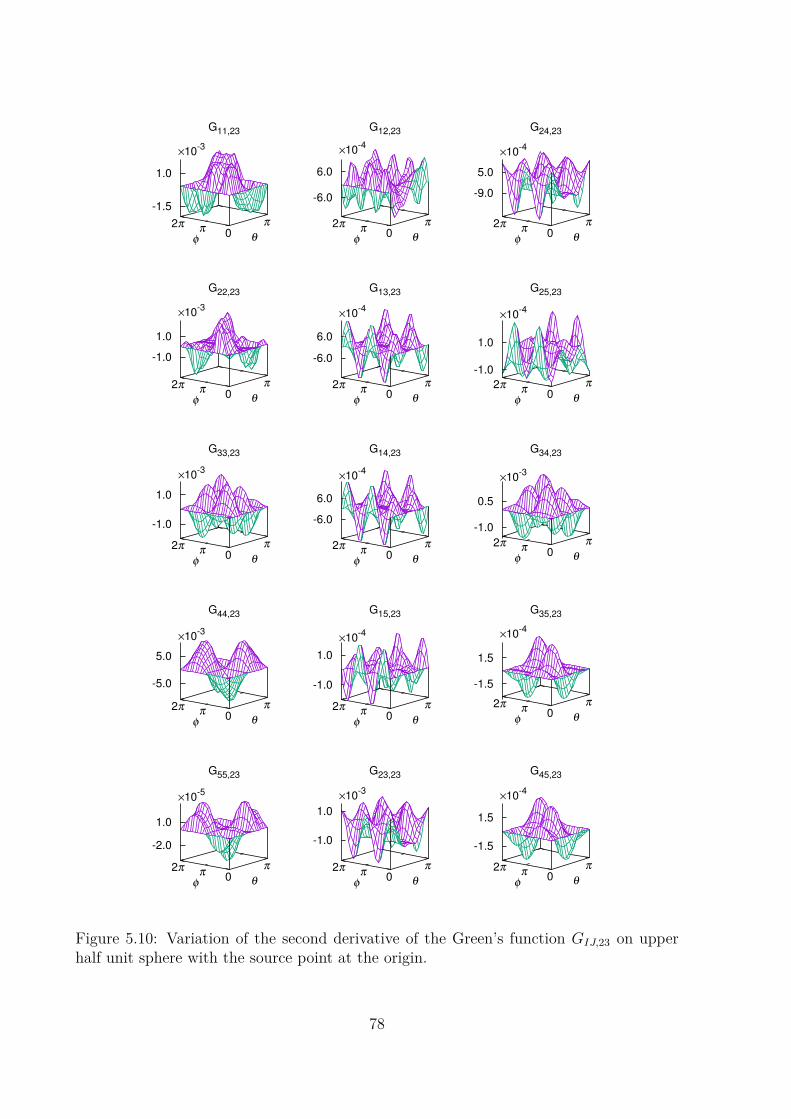
G11,23

×10-3

0

π

θπ2π

φ

-1.5

1.0

G22,23

×10-3

0

π

θπ2π

φ

-1.0

1.0

G33,23

×10-3

0

π

θπ2π

φ

-1.0

1.0

G44,23

×10-3

0

π

θπ2π

φ

-5.0

5.0

G55,23

×10-5

0

π

θπ2π

φ

-2.0

1.0

G12,23

×10-4

0

π

θπ2π

φ

-6.0

6.0

G13,23

×10-4

0

π

θπ2π

φ

-6.0

6.0

G14,23

×10-4

0

π

θπ2π

φ

-6.0

6.0

G15,23

×10-4

0

π

θπ2π

φ

-1.0

1.0

G23,23

×10-3

0

π

θπ2π

φ

-1.0

1.0

G24,23

×10-4

0

π

θπ2π

φ

-9.0

5.0

G25,23

×10-4

0

π

θπ2π

φ

-1.0

1.0

G34,23

×10-3

0

π

θπ2π

φ

-1.0

0.5

G35,23

×10-4

0

π

θπ2π

φ

-1.5

1.5

G45,23

×10-4

0

π

θπ2π

φ

-1.5

1.5

Figure 5.10: Variation of the second derivative of the Green’s function GIJ,23 on upperhalf unit sphere with the source point at the origin.

78

and the orthonormal relation of the eigenvectors. Once the derivatives of the Stroh eigen-vectors are determined, the derivatives of the Green’s function can be constructed fromthem. The accuracy of the present novel explicit expressions of the Green’s function andits derivatives for generally anisotropic magnetoelectroelastic materials is verified by theanalytical solutions for transversely isotropic magnetoelectroelastic materials. The CPUtime for the calculation is provided to show the efficiency of the present novel expressions.For evaluation of the Green’s function and its derivatives in degenerate (identical eigen-values) and nearly degenerate (very close eigenvalues) cases, a small perturbation on thematerial constants is suggested to avoid the presence of the identical or very close Stroheigenvalues.

79

Chapter 6

Applications of the Green’s functionand its derivatives in the BEM

6.1 Preliminary remarks

The boundary element method (BEM) is a general and efficient numerical method formany practical problems. It is sometimes called the boundary integral equation (BIE)method, because the BEM is based on the discretization of the BIE. Some of the ad-vantages of the BEM are (1) the reduction of the dimension of problems to be solved,from three dimension to two dimension, or from two dimension to one dimension, (2) theaccuracy of the BEM due to the nature of integrals used in the formulation, and (3) theeasy and accurate modeling for problems in infinite domain without additional conditionsat infinity due to the properties of the kernel function or the Green’s function.

The BIE method and its numerical evaluation were first formulated to solve the po-tential problems by Jaswon (1963), Jaswon and Ponter (1963) and Symm (1963). LaterRizzo (1967) extended this method to solve the elastic problems. Following these earlyworks, extensive research efforts had been made to use the BIE method as well as theBEM to solve many problems in applied mechanics and engineering. Among the sub-sequent contributions, Cruse (1968, 1974), Cruse and Rizzo (1968), Lachat and Watson(1976), Rizzo and Shippy (1977), Wilson and Cruse (1978), Sladek and Sladek (1982),Tanaka et al. (1994), Aliabadi (1997) and Tan et al. (2013) should be mentioned. Acomprehensive review with recent advances and some future directions of the BEM wasgiven by Liu et al. (2011). A recent overview of the BEM was given by Mukherjee andLiu (2013). For textbooks on the BEM, readers are referred to Aliabadi (2002) and Gaulet al. (2003).

In this chapter, the Green’s function and its derivatives for anisotropic linear elasticmaterials are implemented into a BEM, which serves as a typical application of the Green’sfunction and its derivatives. Some representative numerical examples are presented todemonstrate the correctness and the accuracy of the developed BEM.

81

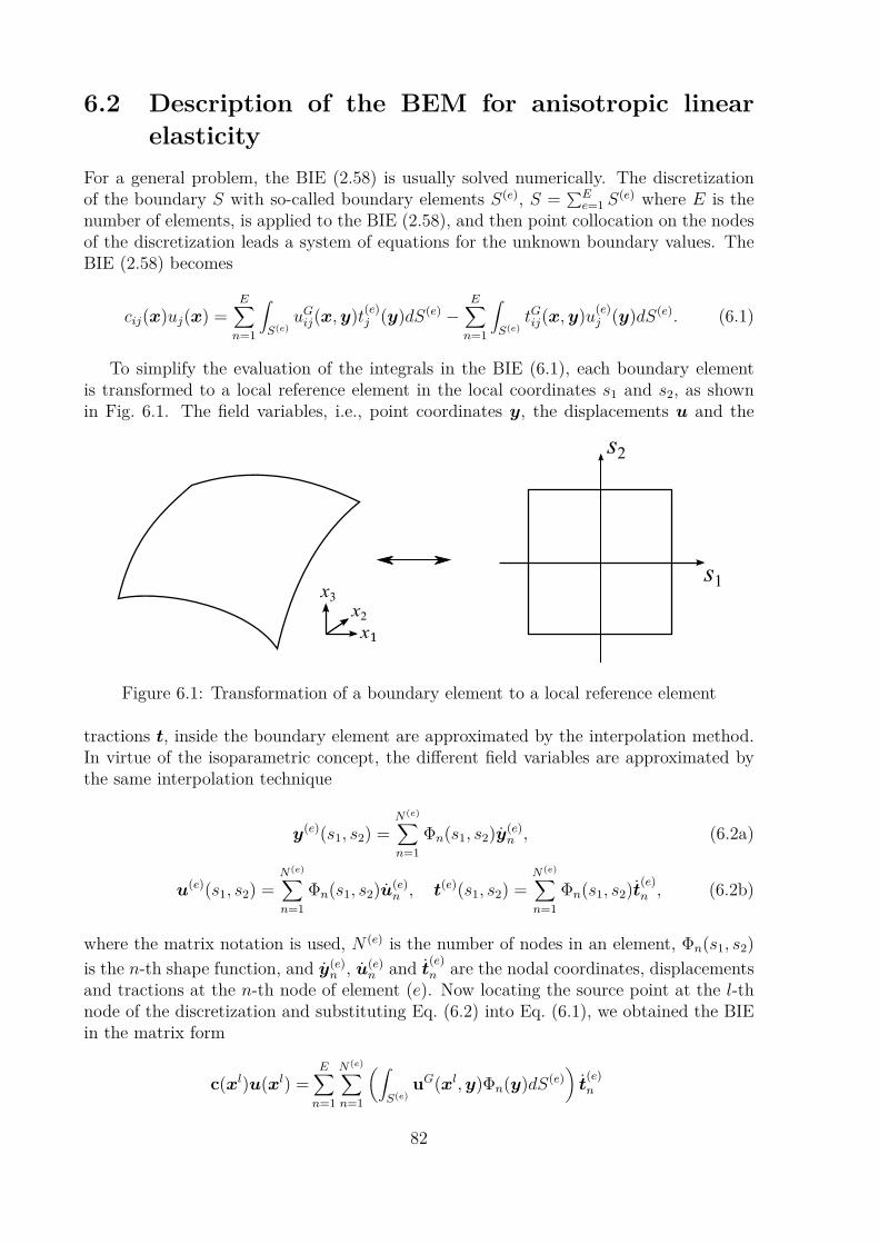
6.2 Description of the BEM for anisotropic linearelasticity

For a general problem, the BIE (2.58) is usually solved numerically. The discretizationof the boundary S with so-called boundary elements S(e), S = ∑E

e=1 S(e) where E is the

number of elements, is applied to the BIE (2.58), and then point collocation on the nodesof the discretization leads a system of equations for the unknown boundary values. TheBIE (2.58) becomes

cij(x)uj(x) =E∑n=1

∫S(e)

uGij(x,y)t(e)j (y)dS(e) −E∑n=1

∫S(e)

tGij(x,y)u(e)j (y)dS(e). (6.1)

To simplify the evaluation of the integrals in the BIE (6.1), each boundary elementis transformed to a local reference element in the local coordinates s1 and s2, as shownin Fig. 6.1. The field variables, i.e., point coordinates y, the displacements u and the

x1

x2x3

s1

s2

Figure 6.1: Transformation of a boundary element to a local reference element

tractions t, inside the boundary element are approximated by the interpolation method.In virtue of the isoparametric concept, the different field variables are approximated bythe same interpolation technique

y(e)(s1, s2) =N(e)∑n=1

Φn(s1, s2)y(e)n , (6.2a)

u(e)(s1, s2) =N(e)∑n=1

Φn(s1, s2)u(e)n , t(e)(s1, s2) =

N(e)∑n=1

Φn(s1, s2)t(e)n , (6.2b)

where the matrix notation is used, N (e) is the number of nodes in an element, Φn(s1, s2)is the n-th shape function, and y(e)

n , u(e)n and t(e)n are the nodal coordinates, displacements

and tractions at the n-th node of element (e). Now locating the source point at the l-thnode of the discretization and substituting Eq. (6.2) into Eq. (6.1), we obtained the BIEin the matrix form

c(xl)u(xl) =E∑n=1

N(e)∑n=1

(∫S(e)

uG(xl,y)Φn(y)dS(e))t

(e)n

82

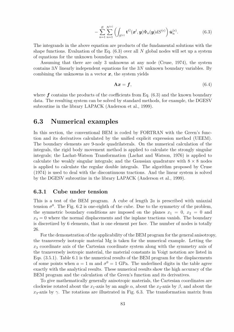
−E∑n=1

N(e)∑n=1

(∫S(e)

tG(xl,y)Φn(y)dS(e))u(e)n . (6.3)

The integrands in the above equation are products of the fundamental solutions with theshape functions. Evaluation of the Eq. (6.3) over all N global nodes will set up a systemof equations for the unknown boundary values.

Assuming that there are only 3 unknowns at any node (Cruse, 1974), the systemcontains 3N linearly independent equations for the 3N unknown boundary variables. Bycombining the unknowns in a vector x, the system yields

Ax = f , (6.4)

where f contains the products of the coefficients from Eq. (6.3) and the known boundarydata. The resulting system can be solved by standard methods, for example, the DGESVsubroutine in the library LAPACK (Anderson et al., 1999).

6.3 Numerical examplesIn this section, the conventional BEM is coded by FORTRAN with the Green’s func-tion and its derivatives calculated by the unified explicit expression method (UEEM).The boundary elements are 9-node quadrilaterals. On the numerical calculation of theintegrals, the rigid body movement method is applied to calculate the strongly singularintegrals; the Lachat-Watson Transformation (Lachat and Watson, 1976) is applied tocalculate the weakly singular integrals; and the Gaussian quadrature with 8 × 8 nodesis applied to calculate the regular double integrals. The algorithm proposed by Cruse(1974) is used to deal with the discontinuous tractions. And the linear system is solvedby the DGESV subroutine in the library LAPACK (Anderson et al., 1999).

6.3.1 Cube under tensionThis is a test of the BEM program. A cube of length 2a is prescribed with uniaxialtension σ0. The Fig. 6.2 is one-eighth of the cube. Due to the symmetry of the problem,the symmetric boundary conditions are imposed on the planes x1 = 0, x2 = 0 andx3 = 0 where the normal displacements and the inplane tractions vanish. The boundaryis discretized by 6 elements, that is one element per face. The number of nodes is totally26.

For the demonstration of the applicability of the BEM program for the general anisotropy,the transversely isotropic material Mg is taken for the numerical example. Letting thex3 coordinate axis of the Cartesian coordinate system along with the symmetry axis ofthe transversely isotropic material, the material constants in Voigt notation are listed inEqs. (3.5.1). Table 6.1 is the numerical results of the BEM program for the displacementsof some points when a = 1 m and σ0 = 1 GPa. The underlined digits in the table agreeexactly with the analytical results. These numerical results show the high accuracy of theBEM program and the calculation of the Green’s function and its derivatives.

To give mathematically generally anisotropic materials, the Cartesian coordinates areclockwise rotated about the x1-axis by an angle α, about the x2-axis by β, and about thex3-axis by γ. The rotations are illustrated in Fig. 6.3. The transformation matrix from

83

a

σ0

x1x2

x3

Figure 6.2: One-eighth of a cube under tension

Points u1 (10−3m) u2 (10−3m) u3 (10−3m)(1.0, 1.0, 1.0) -4.9790686007 -4.9790686007 19.7097507377(0.5, 0.5, 1.0) -2.4895346247 -2.4895346247 19.7097333807(1.0, 0.5, 0.5) -4.9790717447 -2.4895319447 9.85487006790(0.5, 1.0, 0.5) -2.4895319447 -4.9790717447 9.85487006790(1.0, 0.5, 1.0) -4.9790705923 -2.4895335628 19.7097415567(0.5, 1.0, 1.0) -2.4895335628 -4.9790705923 19.7097415567(1.0, 1.0, 0.5) -4.9790558988 -4.9790558988 9.85487214820

Table 6.1: Displacements of the cube under tension with transversely isotropic materialMg

84

x1

x2

x3

α

β

γ

Figure 6.3: Rotations of the coordinates.

the origin system to the new system is

Ω =

cos β cos γ sinα sin β cos γ − cosα sin γ cosα sin β cos γ + sinα sin γcos β sin γ cosα cos γ + sinhα sin β sin γ − sinα cos γ + cosα sin β sin γ− sin β sinα cos β cosα cos β

. (6.5)

Then the elasticity tensor in the new Cartesian coordinate system isc∗ijkl = ΩimΩjnΩksΩltcmnst. (6.6)

When the angles, α, β and γ, are arbitrary, the material constant matrix in Voigt notationin the new coordinate system is generally anisotropic. However, due to the symmetryrequired by the analysis, we choose α = π/2, β = 0 and γ = 0. In this case, the materialconstant matrix is given by

59.7 21.7 26.2 0 0 061.7 21.7 0 0 0

59.7 0 0 016.4 0 0

Sym. 16.75 016.4

(GPa). (6.7)

Table 6.2 are the numerical results of the BEM program with the rotated material Mg,compared with the results of the software COMSOL. The results are accurate, althoughthe number of the elements is small.

6.3.2 Cube with a spheroidal cavity under tensionIn this example, we consider a cube of length 2a under tension σ0 with a small spheroidcavity in the center. Fig. 6.4 (a) is the cube and Fig. 6.4 (b) is one-eighth of it, which

85

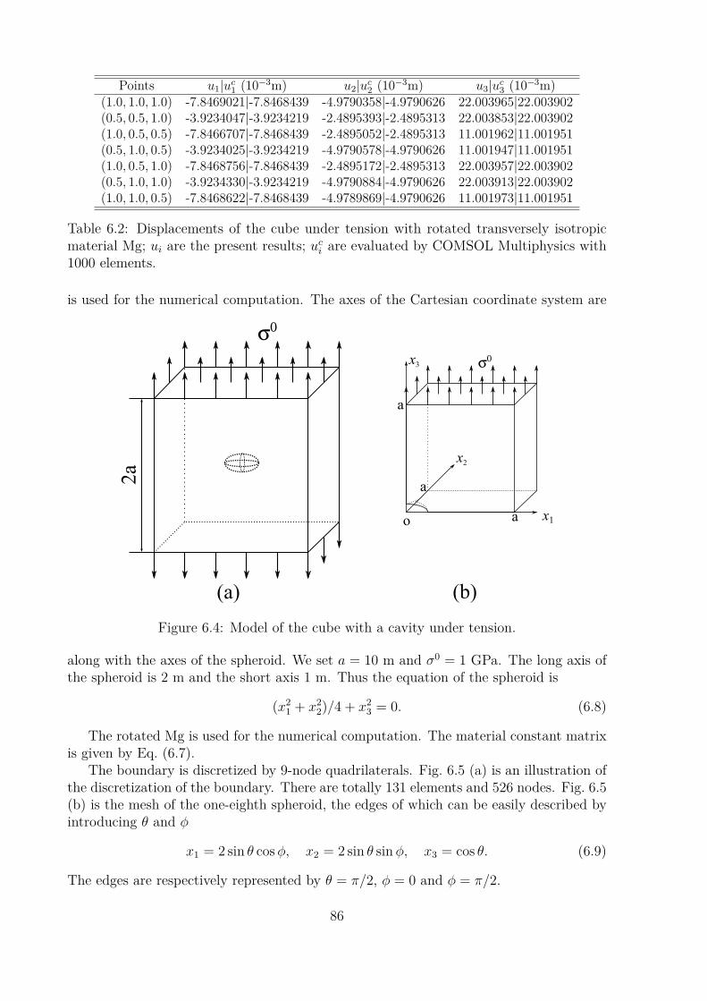
Points u1|uc1 (10−3m) u2|uc2 (10−3m) u3|uc3 (10−3m)(1.0, 1.0, 1.0) -7.8469021|-7.8468439 -4.9790358|-4.9790626 22.003965|22.003902(0.5, 0.5, 1.0) -3.9234047|-3.9234219 -2.4895393|-2.4895313 22.003853|22.003902(1.0, 0.5, 0.5) -7.8466707|-7.8468439 -2.4895052|-2.4895313 11.001962|11.001951(0.5, 1.0, 0.5) -3.9234025|-3.9234219 -4.9790578|-4.9790626 11.001947|11.001951(1.0, 0.5, 1.0) -7.8468756|-7.8468439 -2.4895172|-2.4895313 22.003957|22.003902(0.5, 1.0, 1.0) -3.9234330|-3.9234219 -4.9790884|-4.9790626 22.003913|22.003902(1.0, 1.0, 0.5) -7.8468622|-7.8468439 -4.9789869|-4.9790626 11.001973|11.001951

Table 6.2: Displacements of the cube under tension with rotated transversely isotropicmaterial Mg; ui are the present results; uci are evaluated by COMSOL Multiphysics with1000 elements.

is used for the numerical computation. The axes of the Cartesian coordinate system are

2a

σ0

(a)

o x1

x2

x3 σ0

a

a

a

(b)

Figure 6.4: Model of the cube with a cavity under tension.

along with the axes of the spheroid. We set a = 10 m and σ0 = 1 GPa. The long axis ofthe spheroid is 2 m and the short axis 1 m. Thus the equation of the spheroid is

(x21 + x2

2)/4 + x23 = 0. (6.8)

The rotated Mg is used for the numerical computation. The material constant matrixis given by Eq. (6.7).

The boundary is discretized by 9-node quadrilaterals. Fig. 6.5 (a) is an illustration ofthe discretization of the boundary. There are totally 131 elements and 526 nodes. Fig. 6.5(b) is the mesh of the one-eighth spheroid, the edges of which can be easily described byintroducing θ and φ

x1 = 2 sin θ cosφ, x2 = 2 sin θ sinφ, x3 = cos θ. (6.9)

The edges are respectively represented by θ = π/2, φ = 0 and φ = π/2.

86

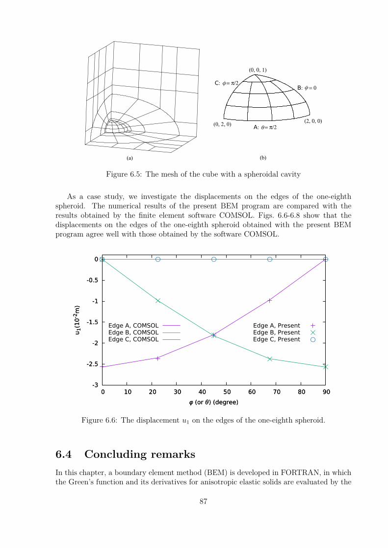
(0, 2, 0)

C: = π/2B: = 0

A: = π/2(2, 0, 0)

(0, 0, 1)

𝜃

𝜙𝜙

(a) (b)

Figure 6.5: The mesh of the cube with a spheroidal cavity

As a case study, we investigate the displacements on the edges of the one-eighthspheroid. The numerical results of the present BEM program are compared with theresults obtained by the finite element software COMSOL. Figs. 6.6-6.8 show that thedisplacements on the edges of the one-eighth spheroid obtained with the present BEMprogram agree well with those obtained by the software COMSOL.

-3

-2.5

-2

-1.5

-1

-0.5

0

0 10 20 30 40 50 60 70 80 90

u1(1

0-2

m)

φ (or θ) (degree)

Edge A, PresentEdge B, PresentEdge C, Present

-3

-2.5

-2

-1.5

-1

-0.5

0

0 10 20 30 40 50 60 70 80 90

u1(1

0-2

m)

φ (or θ) (degree)

Edge A, COMSOLEdge B, COMSOLEdge C, COMSOL

Figure 6.6: The displacement u1 on the edges of the one-eighth spheroid.

6.4 Concluding remarksIn this chapter, a boundary element method (BEM) is developed in FORTRAN, in whichthe Green’s function and its derivatives for anisotropic elastic solids are evaluated by the

87

-2.5

-2

-1.5

-1

-0.5

0

0.5

0 10 20 30 40 50 60 70 80 90

u2(1

0-2

m)

φ (or θ) (degree)




-1

0

1

2

3

4

5

6

7

8

0 10 20 30 40 50 60 70 80 90

u3(1

0-2

m)

φ (or θ) (degree)




88

unified explicit expressions method (UEEM). The program is tested by a problem whichhas analytical solutions. The numerical results suggested the correctness of the codedBEM program and therefore the correctness of the Green’s function and its derivatives.Then the BEM program is used to solve the problem of a cube with a spheroid cavity inthe center under tension. The results agree well with the numerical results by the FEMsoftware COMSOL. So the present BEM can be used for general structural analysis in 3Danisotropic elasticity.

89

Chapter 7

Summary and outlook

Novel explicit expressions of the 3D Green’s function and its derivatives for linear elastic,piezoelectric and magnetoelectroelastic materials are presented and investigated in thisthesis. The starting point for deriving the explicit expressions of the Green’s function andits derivatives is the line integral expression of the Green’s function and its derivatives,which can be derived by applying the Fourier transform or Radon transform followed bysome elementary mathematical manipulations to the governing equations for the Green’sfunction. A straightforward way to derive the explicit expressions is applying the residuecalculus to the line integrals, which is referred to as the residue calculus method (RCM)in this thesis. An alternative way is to construct the explicit expressions in terms of thesolutions of a standard eigenvalue problem, or Stroh eigenvalue problem. This methodis referred to as the Stroh formalism method (SFM) in this thesis. However, the numer-ical evaluation of the RCM and SFM has some troubles in the degenerate and nearlydegenerate cases when the Stroh eigenvalues or the roots of the characteristic equationare identical or very close to each other. By a proper rewritten of the explicit expressionsresulting from the residue calculus, novel unified explicit expressions of the Green’s func-tion and its derivatives are obtained. Here, unified means that the explicit expressionskeep the same form and are applicable for all cases including non-degenerate, nearly de-generate and degenerate cases. The serious difficulty arising in the numerical evaluationof the RCM and SFM doesn’t occur in the numerical evaluation of the unified explicitexpressions. This method is referred to as unified explicit expression method (UEEM) inthis thesis.

The derivations of the explicit expressions of the Green’s function and its derivativesfor anisotropic linear elastic materials by the three methods as well as the numerical in-tegration method (NIM) are presented in Chapter 3. For the numerical computation, theRCM and SFM require a small perturbation on the material constants to avoid the nearlydegenerate and degenerate cases in order to keep a general evaluation procedure for theGreen’s function and its derivatives, while the UEEM does not has such a requirement.The accuracy and efficiency of the three methods, as well as the NIM, are compared witheach other. It is shown that the UEEM exhibits the highest accuracy and efficiency for thenumerical evaluation of the Green’s function and its derivatives for the anisotropic linearelastic materials. However, due to the mathematical complexity, the UEEM is difficult tobe extended directly to the derivative evaluations of the Green’s function for the linearpiezoelectric and magnetoelectroelastic materials. For this reason, in Chapter 4, only theRCM and SFM are directly extended to derive the explicit expressions of the Green’s func-

91

tion and its derivatives for the anisotropic linear piezoelectric materials. By the numericalevaluations of these two methods, it is shown that 1) if similar accuracy is required, theSFM is more efficient than the RCM, and 2) to retain a generally valid evaluation pro-cedure, the required perturbation of the material constants by the SFM is smaller thanthat by the RCM. Thus, only the SFM is extended to derive the explicit expressions ofthe Green’s function and its derivatives for the anisotropic linear magnetoelectroelasticmaterials in Chapter 5. As representative applications, the UEEM is implemented into aboundary element method (BEM) FORTRAN-program for anisotropic linear elastic ma-terials. The numerical examples by using the developed BEM program in Chapter 6 showthe correctness and accuracy of the implemented BEM program in this work. Therefore,the potential applications of the UEEM in the BEM programming are demonstrated.

As future research works, the UEEM should be extended to the linear piezoelectricand magnetoelectroelastic materials, because it is in all likelihood the most efficient andaccurate one among the three aforementioned methods with explicit expressions. Be-sides, the implementations of different explicit expressions of the Green’s function andits derivatives for linear piezoelectric and magnetoelectroelastic materials into the BEMshould be conducted in future.

92

Appendix A

Residue calculus of an improper lineintegral

In the complex analysis, the Cauchy residue theorem is a powerful tool to calculate thecontour integrals, i.e., the line integrals defined over closed curves; it can be used toevaluate real integrals as well. In the complex plane, the equation of Cauchy residuetheorem is ∮

γf(z)dz = 2πi

∑Res(f, pk), (A.1)

where γ is a closed curve, variables pk are poles of the function f(z) inside the curve γ,and Res(f, pk) is the residue of the function f(z) at a pole pk. If pk is a pole of m-order,then

Res(f, pk) = 1(m− 1)! lim

p→pk

dm−1

dpm−1 [(p− pk)mf(p)]. (A.2)

The integral ∫ +∞

−∞f(x)dx, (A.3)

where f(x) = ∑mk=0 bkx

k/∑nk=0 akx

k with an 6= 0 and n > m, arises in the study ofthe Green’s function for the general anisotropic materials. It resists the techniques ofelementary calculus but can be evaluated as a limit of a contour integral in the complexplane. As illustrated in Fig. A.1, the contour goes along the real line from A to B, andthen counterclockwise along a semicircle centered at the origin from B to A through C.The radius ξ of the semicircle is large enough to allow the semicircle includes all poleswith positive imaginary parts. The contour integral is

∮Γ f(z)dz. Since the contour can

be divided into a straight line AB and an arc BCA, we have∮Γf(z)dz =

∫AB

f(z)dz +∫BCA

f(z)dz = 2πi∑

Res(f, pk), Im(pk) > 0. (A.4)

When z is on the straight line AB, the integral on the line is∫AB

f(z)dz =∫ +ξ

−ξf(x)dx (A.5)

When z is on the arc BCA, substitution of z = x+ yi = ξeiθ into f(z) leads to∫BCA

f(z)dz =∫ π

0

∑mk=0 bkξ

kekθi∑nk=0 akξ

kekθidθ. (A.6)

93

x

y

A(−ξ, 0) B(+ξ, 0)

C(0, ξ)

Γ

z = x+ yi

Figure A.1: The contour Γ.

When ξ → ∞, the integrand of the right integral in Eq. (A.6) vanish since n > m whileθ is independent of ξ. Therefore limξ→∞

∫BCA f(z)dz = 0. Then we have∫ +∞

−∞f(x)dx = 2πi

∑Res(f, pk), Im(pk) > 0. (A.7)

Some literature on the explicit evaluation of the Green’s function by the residue cal-culus had directly given the above equation. We give the proof here for the reader’sconvenience to understand Eq. (A.7), which will be used in the following chapters.

94

Appendix B

Explicit expressions of N,i and N,ij

In this appendix, the derivatives of N for elastic, piezoelectric and magnetoelectroelasticmaterials are presented in a unified form.

Given any two orthogonal unit vectors n and m on the oblique plane perpendicularto x, N is defined as

N =(

N1 N2N3 NT

1

), (B.1)

N1 = −T−1RT , N2 = T−1 = NT2 , N3 = RT−1RT −Q,

withQIJ = CkIJlnknl, RIJ = CkIJlnkml, TIJ = CkIJlmkml, (B.2)

where the repeated lowercase letters denote summation from 1 to 3, and the capital lettersI and J are from 1 to 3 in elasticity, from 1 to 4 in piezoelectricity, and from 1 to 5 inmagnetoelectroelasticity. In the program, it is convenience to note that

N2 = T−1, N1 = −N2RT , N3 = −RN1 −Q. (B.3)

The derivatives of N mainly consist of the derivatives of N1, N2 and N3. Since (T−1),i =−T−1T,iT−1, which can be obtained by taking the derivative of T−1T = I, the firstderivatives of N1, N2 and N3 are

N2,i = −N2T,iN2, N1,i = −N2,iRT −N2RT,i , N3,i = −R,iN1 −RN1,i −Q,i. (B.4)

The second derivative is obtained by taking an additional the derivative of the first deriva-tive, i.e.,

N2,ij = −N2,jT,iN2 −N2T,ijN2 −N2T,iN2,j,

N1,ij = −N2,ijRT −N2,iRT,j −N2,jRT

,i −N2RT,ij, (B.5)

N3,ij = −R,ijN1 −R,iN1,j −R,jN1,i −RN1,ij −Q,ij.

The derivatives of Q, R and T are expressed in terms of n andm and their derivativeswhich are presented in the following after a proper choice of n and m.

For any point except x1 = x2 = 0, n and m are chosen as

n = 1ρ

[−x2, x1, 0] , m = 1ρr

[−x1x3,−x2x3, x

21 + x2

2

], (B.6a)

95

whereρ =

√x2

1 + x22, r =

√x2

1 + x22 + x2

3. (B.6b)

The non-zero derivatives of ρ and r are

ρ,i = xi/ρ, ρ,ij = (δij − ρ,iρ,j)/ρ, i, j 6= 3,r,i = xi/r, r,ij = (δij − r,ir,j)/r. (B.7)

Introducing

n = [−x2, x1, 0] , m =[−x1x3,−x2x3, x

21 + x2

2

], (B.8)

the derivatives of n and m are given by

n,i = (n,i − ρ,in)/ρ,n,ij = −(ρ,ijn+ ρ,in,j + ρ,jn,i)/ρ, (B.9a)m,i = [m,i − (ρr),im] /(ρr),

m,ij = [m,ij − (ρr),ijm− (ρr),im,j − (ρr),jm,i] /(ρr),

where

(ρr),i = ρ,ir + ρr,i,

(ρr),ij = ρ,ijr + ρ,ir,j + ρ,jr,i + ρr,ij,

n,i = [−δ2i, δ1i, 0] , n,ij = 0,m,i = [−δ1ix3 − δ3ix1,−δ2ix3 − δ3ix2, 2x1δ1i + 2x2δ2i] ,

m,ij = [−δ1iδ3j − δ3iδ1j,−δ2iδ3j − δ3iδ2j, 2δ1iδ1j + 2δ2iδ2j] . (B.9b)

Another possible choice for the orthogonal vectors n and m is

n = 1ρ

[−x3, 0, x1] , m = 1ρr

[−x1x2, x

21 + x2

3,−x2x3], (B.10a)

whereρ =

√x2

1 + x23, r =

√x2

1 + x22 + x2

3. (B.10b)

Note that this choice is applicable everywhere except on the line x1 = x3 = 0, and weapply it at points x1 = x2 = 0, x3 6= 0 which are excluded in the previous choice forvectors n and m. Following the previous procedure, when x1 = x2 = 0, most componentsof the derivatives of n and m are zero except the following ones

n3,1 = 1/|x3|, n1,11 = sgn(x3)/x23,

n3,13 = n3,31 = −sgn(x3)/x23,

m3,2 = −1/x3, m1,12 = m1,21 = −1/x23,

m2,22 = −1/x23, m3,23 = m3,32 = 1/x2

3. (B.11)

By using the above given relations, the explicit expressions for the derivatives of Ncan be obtained.

96

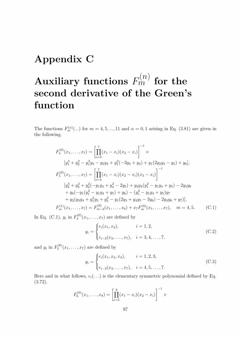
Appendix C

Auxiliary functions F (n)m for the

second derivative of the Green’sfunction

The functions F (α)m (...) for m = 4, 5, ..., 11 and α = 0, 1 arising in Eq. (3.81) are given in

the following.

F(0)4 (x1, . . . , x7) =

[ 7∏i=3

(x1 − xi)(x2 − xi)]−1

×

[y41 + y2

2 − y31y3 − y2y4 + y2

1(−3y2 + y4) + y1(2y2y3 − y5) + y6],

F(0)5 (x1, . . . , x7) =

[ 7∏i=4

(x1 − xi)(x2 − xi)(x3 − xi)]−1

[y32 + y2

3 + y22(−y1y4 + y2

4 − 2y5) + y3y4(y21 − y1y4 + y5)− 2y3y6

+ y6(−y1(y21 − y1y4 + y5) + y6)− (y2

1 − y1y4 + y5)y7

+ y2(y3y4 + y21y5 + y2

5 − y1(2y3 + y4y5 − 3y6)− 2y4y6 + y7)],F (1)m (x1, . . . , x7) = F

(0)m−2(x1, . . . , x6) + x7F

(0)m (x1, . . . , x7), m = 4, 5. (C.1)

In Eq. (C.1), yi in F(0)4 (x1, . . . , x7) are defined by

yi =

ei(x1, x2), i = 1, 2,

ei−2(x3, . . . , x7), i = 3, 4, . . . , 7,(C.2)

and yi in F(0)5 (x1, . . . , x7) are defined by

yi =

ei(x1, x2, x3), i = 1, 2, 3,

ei−3(x4, . . . , x7), i = 4, 5, . . . , 7.(C.3)

Here and in what follows, ei(. . .) is the elementary symmetric polynomial defined by Eq.(3.72).

F(0)6 (x1, . . . , x8) =

[ 8∏i=3

(x1 − xi)(x2 − xi)]−1

×

97

[y51 − y4

1y3 + y31(−4y2 + y4) + y2

1(3y2y3 − y5)+ y2(−y2y3 + y5) + y1(3y2

2 − 2y2y4 + y6)− y7], (C.4a)

F(0)7 (x1, . . . , x8) =

[ 8∏i=4

(x1 − xi)(x2 − xi)(x3 − xi)]−1

×

[y42 + y2

3y24 + y3

2(−y1y4 + y24 − 2y5)− y2

3y5 + y3y5y6 + y41y7 − 2y3y4y7

+ y22(y3y4 + y2

1y5 + y25 − y1(3y3 + y4y5 − 3y6)− 2y4y6 + 2y7) + y3y8

+ y31(y8 − y3y5 − y4y7) + y2

1(y23 + y3y4y5 + y5y7 − y4y8)− y6y8

+ y27 − y1(2y2

3y4 + y3(y25 − 3y7) + y6y7 − y5y8) + y2(2y2

3 − 2y5y7

+ y3(2y1(y1 − y4)y4 + (2y1 + y4)y5 − 3y6) + y26 + y2

1(y4y6 − 4y7)− y1(y5y6 − 3y4y7 + 2y8)− y3

1y6 + y4y8)], (C.4b)

F(0)8 (x1, . . . , x8) =

[ 8∏i=5

(x1 − xi)(x2 − xi)(x3 − xi)(x4 − xi)]−1

×

[y33 + y2

2y4y5 − y24y5 + y2y4y

35 − 2y2y4y5y6 + y4y5y

26 − y3

2y7 + 2y2y4y7

− y22y

25y7 − y4y

25y7 + 2y2

2y6y7 − 2y4y6y7 + 2(y4y5 + (−y2 + y6)y7)y8

− y23(y2y5 − y1y

25 + y3

5 + 2y1y6 − 3y5y6 + 3y7)− y2y26y7 + 2y2y5y

27

+ y21(y4(y5y6 − 2y7)− y7(y2y6 + y5y7) + (y5(y2 + y6) + y7)y8)− y3

7

+ y1(y24 − y4y5(y5(y2 + y6)− 3y7) + y7(y2

2y5 + y2y5y6 − 3y2y7 + y6y7)− 2y4y8 − (y2

2 + y2(y25 − 2y6) + y2

6 + y5y7)y8 + y28) + y3(−y4y

25 + y2

2y6

+ 2y4y6 + y36 − 3y5y6y7 + 3y2

7 − y2(2y4 + y1y5y6 − y25y6 + 2y2

6 − 3y1y7

+ y5y7 − 2y8) + 2y25y8 − 2y6y8 + y2

1(y26 − 2y5y7 + y8)

+ y1(y4y5 + 2y25y7 + y6y7 − y5(y2

6 + 3y8)))− y5y28 + y3

1(y27 − y6y8)], (C.4c)

F (1)m (x1, . . . , x8) = F

(0)m−2(x1, . . . , x7) + x8F

(0)m (x1, . . . , x8), m = 6, 7,

F(1)8 (x1, . . . , x8) = F

(0)5 (x5, x6, x7, x1, . . . , x4) + x8F

(0)8 (x1, . . . , x8). (C.4d)

In Eq. (C.4), yi in F(0)6 (x1, . . . , x8) are defined by

yi =

ei(x1, x2), i = 1, 2,

ei−2(x3, . . . , x8), i = 3, 4, . . . , 8,(C.5)

yi in F(0)7 (x1, . . . , x8) are defined by

yi =

ei(x1, x2, x3), i = 1, 2, 3,

ei−3(x4, . . . , x8), i = 4, 5, . . . , 8,(C.6)

and yi in F(0)8 (x1, . . . , x8) are defined by

yi =

ei(x1, . . . , x4), i = 1, 2, 3, 4,

ei−4(x5, . . . , x8), i = 5, 6, 7, 8.(C.7)

98

F(0)9 (x1, . . . , x9) =

[ 9∏i=3

(x1 − xi)(x2 − xi)]−1

×

[y61 − y5

1y3 + y41(−5y2 + y4) + y3

1(4y2y3 − y5) + y21(6y2

2 − 3y2y4 + y6)− y2(y2

2 − y2y4 + y6)− y1(3y22y3 − 2y2y5 + y7) + y8], (C.8a)

F(0)10 (x1, . . . , x9) =

[ 9∏i=4

(x1 − xi)(x2 − xi)(x3 − xi)]−1

×

[y52 + y3

3y4 + y42(y2

4 − y1y4 − 2y5) + y23y

25 − y2

3y4y6 − y23y7 + y3y6y7 + y2

8

+ y32(y3y4 + y2

1y5 + y25 − y1(4y3 + y4y5 − 3y6)− 2y4y6 + 2y7)− y5

1y8

− 2y3y5y8 − y7y9 + y21(y2

3(y24 + y5) + y3(y5y6 − 4y8) + y6y8 − y5y9)

+ y22(3y2

3 + y3(3y1(y1 − y4)y4 + (4y1 + y4)y5 − 3y6)− y31y6 + y2

6

+ y21(y4y6 − 4y7)− 2y5y7 + 2y4y8 − y1(y5y6 − 3y4y7 + 5y8)− y9)

− y31(y3y4(y3 + y6) + y5y8 − y4y9) + y4

1(y3y6 + y4y8 − y9) + y3y4y9

− y1(2y33 + y2

3(2y4y5 − 3y6) + y7y8 − y6y9 + y3(y26 − 3y4y8 + 2y9))

+ y2(y23(2y2

4 − 3y5) + y41y7 + y2

7 − y31(2y3y5 + y4y7 − 5y8)− 2y6y8

+ y5y9 + y21(3y2

3 + 2y3y4y5 − 3y3y6 + y5y7 − 4y4y8 + 3y9)− y1(4y2

3y4 + 2y3(y25 − y4y6 − 2y7) + y6y7 − 3y5y8 + 2y4y9)

+ y3(y5y6 − 3y4y7 + 4y8))], (C.8b)

F(0)11 (x1, . . . , x9) =

[ 9∏i=5

(x1 − xi)(x2 − xi)(x3 − xi)(x4 − xi)]−1

×

[y43 − y3

4 + y21y

24y

25 − y1y

24y

35 − y2

1y24y6 + y1y

24y5y6 + y2

4y25y6 − y2

4y26

− 2y24y5y7 + y3

1y4y6y7 − y21y4y5y6y7 + y1y4y

26y7 − y4y6y

27 + 3y2

4y8

− y33(y2y5 − y1y

25 + y3

5 + 2y1y6 − 3y5y6 + 3y7) + y42y8 + 2y2

1y4y25y8

+ y21y4y6y8 − 3y1y4y5y6y8 + y4y

26y8 + 2y4y5y7y8 + y4

1y28 − 3y4y

28

− y1y7y28 + y3

8 + (−y41y7 + y3

1(y4 + y5y7 + y8)− y21(3y4y5 + y6y7

+ y5y8) + y1(y4(2y25 + y6) + y2

7 + y6y8)− 2(y4y5y6 − y4y7 + y7y8))y9

+ (y21 − y1y5 + y6)y2

9 + y32(y5(−y1 + y5)y8 − y6(y4 + 2y8) + y1y9)

+ y22(y2

4 + y4y6((y1 − y5)y5 + 2y6)− 3y4y8 + y8(y6(y21 − y1y5 + y6)

+ (3y1 − 2y5)y7 + 2y8) + y1(−y1y5 + y25 − 2y6)y9) + y2

3(−y4y25 + y2

2y6

+ 2y4y6 + y36 − 3y5y6y7 + 3y2

7 − y2(3y4 + y1y5y6 − y25y6 + 2y2

6 − 3y1y7

+ y5y7 − 4y8) + 3y25y8 − 3y6y8 + y2

1(y26 − 2y5y7 + 2y8)− 2y5y9

+ y1(y4y5 + 2y25y7 + y6y7 − y5(y2

6 + 5y8) + 3y9)) + y2(y8(y27 − 2y6y8)

+ y21(3y4y8 − y4y

26 + y5y7y8 − 4y2

8 − y5y6y9 + 3y7y9) + y31(y6y9 − y7y8)

− y4(y36 + 2y2

5y8 − 2y6(y5y7 + y8)) + y24y

25 + y1(y4y5y

26 − y6y7y8

− 2y24y5 − 3y4y6y7 + y4y5y8 + 3y5y

28 + (y4 + y2

6 − 2y5y7 − 3y8)y9)− y2

9 + 2y5y8y9) + y3(y4y5y26 − y2

4y5 − y32y7 − 2y4y

25y7 − y4y6y7 − y3

7

99

+ 4y4y5y8 + 3y6y7y8 − 3y5y28 + 3y5y6y9 − 2(y4 + y2

6 − y5y7 − y8)y9

+ y22(2y4y5 − y2

5y7 + 2y6y7 + y5y8 − 2y9) + y31(y2

7 − 2y6y8 + y5y9)+ y2(2y5y

27 − y2

6y7 + y4(2y35 − 5y5y6 + 3y7) + y5y6y8 − 5y7y8 − 2y2

5y9

+ 4y6y9) + y21(y4y5y6 − 3y4y7 − y2y6y7 − y5y

27 + 3y2y5y8 + 2y5y6y8

+ y7y8 − (2y2 + y25 + 2y6)y9) + y1(2y2

4 + y6y27 + y2

2(y5y7 − 4y8)− 2y2

6y8 − y5y7y8 + 4y28 − y4(2y2(y2

5 − y6) + y25y6 − 5y5y7 + 6y8)

− 4y7y9 + y2(y5y6y7 − 3y27 − 3y2

5y8 + 4y6y8 + 3y5y9)))+ y1y

24y7 − 2y3

1y4y5y8 − y31y5y

28 + y2

1y6y28]

F (1)m (x1, . . . , x9) = F

(0)m−3(x1, . . . , x8) + x9F

(0)m (x1, . . . , x9), m = 9, 10, 11. (C.9)

In Eq. (C.9), yi in F(0)9 (x1, . . . , x9) are defined as

yi =

ei(x1, x2), i = 1, 2,

ei−2(x3, . . . , x9), i = 3, 4, . . . , 9,(C.10)

yi in F(0)10 (x1, . . . , x9) are defined as

yi =

ei(x1, x2, x3), i = 1, 2, 3,

ei−3(x4, . . . , x9), i = 4, 5, . . . , 9,(C.11)

and yi in F(0)11 (x1, . . . , x9) are defined as

yi =

ei(x1, . . . , x4), i = 1, 2, 3, 4,

ei−4(x5, . . . , x9), i = 5, 6, . . . , 9.(C.12)

It should be mentioned here that yi in different F (α)m (...) have different definitions.

100

Appendix D

Explicit expression of the Stroheigenvector ξ

In this appendix, we list the explicit expressions of the Stroh eigenvectors ξ, i.e., a andb. Note that the notations in this appendix follow those in Ref. Hwu (2010). For moredetails, please refer to Ref. Hwu (2010).

The explicit expressions of a and b are given by

a =

a1a2a3a4

=

p1b2 + q1b3 + r1b4

(p2b2 + q2b3 + r2b4) /µ(p4b2 + q4b3 + r4b4) /µp4b2 + q7b3 + r7b4

, (D.1a)

where

pj = µ2S′Dj1 + S

′Dj2 − µS

′Dj6 ,

qj = S′Dj4 − µS

′Dj5 ,

rj = S′Dj8 − µS

′Dj7 , j = 1, 2, 4, 7, (D.1b)

and

b =

b1b2b3b4

= c

µl∗4−l∗4l∗3m∗3

, or c

µl∗3−l∗3l∗2m∗2

, or c

µm∗3−m∗3m∗2ρ∗2

. (D.2)

In Eq. (D.2),

l∗2 = l4ρ2 −m23, l∗3 = m2m3 − l3ρ2, l∗4 = l2ρ2 −m2

2,

m∗2 = l3m3 − l4m2, m∗3 = l3m2 − l2m3, ρ∗2 = l2l4 − l23, (D.3)

where

l2 = S′D55 µ

2 − 2S ′D45 µ+ S

′D44 ,

l3 = S′D15 µ

3 −(S

′D14 + S

′D56

)µ2 +

(S

′D25 + S

′D46

)µ− S ′D

24 ,

l4 = S′D11 µ

4 − 2S ′D16 µ

3 +(2S ′D

12 + S′D66

)µ2 − 2S ′D

26 µ+ S′D22 ,

m2 = g′

15µ2 −

(g

′

14 + g′

25

)µ+ g

′

24,

101

m3 = g′

11µ3 −

(g

′

21 + g′

16

)µ2 +

(g

′

12 + g′

26

)µ− g′

22,

ρ2 = −β ′σ11µ

2 + 2β ′σ12µ− β

′σ22. (D.4)

In the above equations, S ′Dij , g′

ij and β ′σij are the reduced piezoelectric compliances, and µ

represents the Stroh eigenvalues which are the roots of

l2l4ρ2 + 2l3m2m3 − l2m23 − l4m2

2 − ρ2l23 = 0. (D.5)

In Eq. (D.2) c is the scaling factor. To have a unique value for the eigenvectors, for eachStroh eigenvalue µk the scaling factor ck is determined by

c2k = 1

2(a1kb1k + a2kb2k + a3kb3k + a4kb4k), k = 1, 2, 3, 4, (D.6)

where ajk and bjk are the components of a and b before scaling.

102

Bibliography

M. Akamatsu and K. Tanuma. Green’s function of anisotropic piezoelectricity. Proceedingsof the Royal Society of London A: Mathematical, Physical and Engineering Sciences,453(1958):473–487, 1997.

M. H. Aliabadi. A new generation of boundary element methods in fracture mechanics.International Journal of Fracture, 86(1-2):91–125, 1997.

M. H. Aliabadi. The Boundary Element Method: Applications in Solids and Structures,Vol. 2. John Wiley & Sons, New York, 2002.

V. I. Alshits, A. N. Darinskii, and J. Lothe. On the existence of surface waves in half-infinite anisotropic elastic media with piezoelectric and piezomagnetic properties. WaveMotion, 16(3):265–283, 1992.

E. Anderson, Z. Bai, C. Bischof, S. Blackford, J. Demmel, J. Dongarra, J. Du Croz,A. Greenbaum, S. Hammerling, A. McKenney, et al. LAPACK Users’ Guide, volume 9.SIAM, 1999.

D. M. Barnett. The precise evaluation of derivatives of the anisotropic elastic Green’sfunctions. Physica Status Solidi (b), 49(2):741–748, 1972.

D. M. Barnett and J. Lothe. Dislocations and line charges in anisotropic piezoelectricinsulators. Physica Status Solidi (b), 67(1):105–111, 1975.

Y. Benveniste. Magnetoelectric effect in fibrous composites with piezoelectric and piezo-magnetic phases. Physical Review B, 51(22):16424, 1995.

F. C. Buroni and A. Saez. Three-dimensional Green’s function and its derivative formaterials with general anisotropic magneto-electro-elastic coupling. Proceedings of theRoyal Society A: Mathematical, Physical and Engineering Science, 466(2114):515–537,2010.

F. C. Buroni and A. Saez. Unique and explicit formulas for Green’s function in three-dimensional anisotropic linear elasticity. ASME Journal of Applied Mechanics, 80:051018–1–14, 2013.

F. C. Buroni, J. E. Ortiz, and A. Saez. Multiple pole residue approach for 3D BEM analysisof mathematical degenerate and non-degenerate materials. International Journal forNumerical Methods in Engineering, 86(9):1125–1143, 2011.

T. Chen. Green’s functions and the non-uniform transformation problem in a piezoelectricmedium. Mechanics Research Communications, 20:271–278, 1993.

103

T. Chen and F.-Z. Lin. Numerical evaluation of derivatives of the anisotropic piezoelectricGreen’s functions. Mechanics Research Communications, 20:501–506, 1993.

M. Chung and T. Ting. The Green function for a piezoelectric piezomagnetic magneto-electric anisotropic elastic medium with an elliptic hole or rigid inclusion. PhilosophicalMagazine Letters, 72(6):405–410, 1995.

T. A. Cruse. The Direct Potential Method in Three Dimensional Elastostatics. Carnegie-Mellon University, Carnegie Institute of Technology, Department of Mechanical Engi-neering, 1968.

T. A. Cruse. An improved boundary-integral equation method for three dimensionalelastic stress analysis. Computers and Structures, 4(4):741–754, 1974.

T. A. Cruse and F. J. Rizzo. A direct formulation and numerical solution of the generaltransient elastodynamic problem. i. Journal of Mathematical Analysis and Applications,22(1):244–259, 1968.

P. H. Dederichs and G. Liebfried. Elastic Green’s function for anisotropic cubic crystals.Physical Review, 188:1175–1183, 1969.

W. F. J. Deeg. The Analysis of Dislocation, Crack, and Inclusion Problems in PiezoelectricSolids. PhD thesis, Standford University, 1980.

H. Ding and A. Jiang. Fundamental solutions for transversely isotropic magneto-electro-elastic media and boundary integral formulation. Science in China Series E: Techno-logical Sciences, 46(6):607–619, 2003.

H. Ding, J. Liang, and B. Chen. Fundamental solutions for transversely isotropic piezo-electric media. Science in China Series A, 7:009, 1996.

M. L. Dunn. Electroelastic Green’s functions for transversely isotropic piezoelectric mediaand their application to the solution of inclusion and inhomogeneity problems. Inter-national Journal of Engineering Science, 32:119–131, 1994.

M. L. Dunn and H. A. Wienecke. Green’s functions for transversely isotropic piezoelectricsolids. International Journal of Solids and Structures, 33(30):4571–4581, 1996.

W. Eerenstein, N. D. Mathur, and J. F. Scott. Multiferroic and magnetoelectric materials.nature, 442(7104):759–765, 2006.

J. D. Eshelby, W. T. Read, and W. Shockley. Anisotropic elasticity with applications todislocation theory. Acta Metallurgica, 1(3):251–259, 1953.

R. Fitzpatrick. Maxwell’s Equations and the Principles of Electromagnetism. INFINITYSCIENCE PRESS LLC, Hingham, 2008.

I. Fredholm. Sur les equations de l’equilibre d’un corps solide elastique. Acta Mathematica,23(1):1–42, 1900.

L. Gaul, M. Kogl, and M. Wagner. Boundary Element Methods for Engineers and Scien-tists. Springer-Verlag Berlin Heidelberg New York, 2003.

104

L. J. Gray, D. Ghosh, and T. Kaplan. Evaluation of the anisotropic Green’s function inthree dimensional elasticity. Computational Mechanics, 17:253–261, 1996.

S. A. Gundersen and J. Lothe. A new method for numerical calculations in anisotropicelasticity problems. Physica Status Solidi (b), 143(1):73–85, 1987.

J. H. Huang and W.-s. Kuo. The analysis of piezoelectric/piezomagnetic composite ma-terials containing ellipsoidal inclusions. Journal of Applied Physics, 81(3):1378–1386,1997.

C. Hwu. Anisotropic Elastic Plates. Springer, New York, 2010.

M. A. Jaswon. Integral equation methods in potential theory. i. Proceedings of the RoyalSociety of London A: Mathematical, Physical and Engineering Sciences, 275(1360):23–32, 1963.

M. A. Jaswon and A. R. Ponter. An integral equation solution of the torsion problem.Proceedings of the Royal Society of London A: Mathematical, Physical and EngineeringSciences, 273(1353):237–246, 1963.

M. A. Jenkins. Algorithm 493: Zeros of a real polynomial [c2]. ACM Transactions onMathematical Software (TOMS), 1(2):178–189, 1975.

M. A. Jenkins and J. F. Traub. A three-stage algorithm for real polynomials usingquadratic iteration. SIAM Journal on Numerical Analysis, 7(4):545–566, 1970.

R. M. Jones. Mechanics of composite materials. Crc Press, 1998.

J. C. Lachat and J. O. Watson. Effective numerical treatment of boundary integralequations: a formulation for three-dimensional elastostatics. International Journal forNumerical Methods in Engineering, 10(5):991–1005, 1976.

A. M. Lavagnino. Selected Static and Dynamic Problems in Anisotropic Linear Elasticity.PhD thesis, Stanford University, Stanford, 1995.

V.-G. Lee. Explicit expression of derivatives of elastic Green’s functions for generalanisotropic materials. Mechanics Research Communications, 30(3):241–249, 2003.

V.-G. Lee. Derivatives of the three-dimensional Green’s functions for anisotropic materi-als. International Journal of Solids and Structures, 46(18):3471–3479, 2009.

J. Y. Li and M. L. Dunn. Anisotropic coupled-field inclusion and inhomogeneity problems.Philosophical Magazine A, 77(5):1341–1350, 1998.

K.-H. C. Lie and J. Koehler. The elastic stress field produced by a point force in a cubiccrystal. Advances in Physics, 17(67):421–478, 1968.

I. M. Lifshitz and L. N. Rozenzweig. Construction of the Green tensor for the fundamentalequation of elasticity theory in the case of unbounded elastically anisotropic medium.Zh. Eksp. Teor. Fiz, 17:783–791, 1947.

105

J. Liu, X. Liu, and Y. Zhao. Green’s functions for anisotropic magnetoelectroelastic solidswith an elliptical cavity or a crack. International Journal of Engineering Science, 39(12):1405–1418, 2001.

Y. J. Liu, S. Mukherjee, N. Nishimura, M. Schanz, W. Ye, A. Sutradhar, E. Pan, N. A.Dumont, A. Frangi, and A. Saez. Recent advances and emerging applications of theboundary element method. Applied Mechanics Reviews, 64(3):030802, 2011.

K. Malen. A unified six-dimensional treatment of elastic Green’s functions and disloca-tions. Physica Status Solidi (b), 44(2):661–672, 1971.

S. Mukherjee and Y. Liu. The boundary element method. International Journal ofComputational Methods, 10(06):1350037, 2013.

T. Mura. Micromechanics of Defects in Solids. Kluwer Academic Pub, 1987.

T. Mura and N. Kinoshita. Green’s functions for anisotropic elasticity. Phys. Status SolidiB, 47:607–618, 1971.

G. Nakamura and K. Tanuma. A formula for the fundamental solution of anisotropicelasticity. Quartely Journal of Mechanics and Applied Mathematics, 50:179–194, 1997.

R. B. Nelson. Simplified calculation of eigenvector derivatives. AIAA journal, 14(9):1201–1205, 1976.

E. Pan. Three-dimensional Green’s functions in anisotropic magneto-electro-elastic bi-materials. Zeitschrift fur angewandte Mathematik und Physik ZAMP, 53(5):815–838,2002.

E. Pan and W. Chen. Static Green’s Functions in Anisotropic Media. Cambridge Univer-sity Press, 2015.

E. Pan and F. Tonon. Three-dimensional Green’s functions in anisotropic piezoelectricsolids. International Journal of Solids and Structures, 37(6):943–958, 2000.

E. Pan and F. G. Yuan. Boundary element analysis of three-dimensional cracks inanisotropic solids. International Journal for Numerical Methods in Engineering, 48:211–237, 2000.

Y.-C. Pan and T.-W. Chou. Point force solution for an infinite transversely isotropic solid.Journal of Applied Mechanics, 43(4):608–612, 1976.

A.-V. Phan, L. J. Gray, and T. Kaplan. On the residue calculus evaluation of the 3Danisotropic elastic Green’s function. Communications in Numerical Methods in Engi-neering, 20(5):335–341, 2004.

A.-V. Phan, L. J. Gray, and T. Kaplan. Residue approach for evaluating the 3Danisotropic elastic Green’s function: Multiple roots. Engineering Analysis with Bound-ary Elements, 29(6):570–576, 2005.

W. H. Press. Numerical Recipes 3rd Edition: The Art of Scientific Computing. CambridgeUniversity Press, 2007.

106

Q.-H. Qin. Green’s functions of magnetoelectroelastic solids with a half-plane boundaryor bimaterial interface. Philosophical Magazine Letters, 84(12):771–779, 2004.

Q.-H. Qin. Green’s Function and Boundary Elements of Multifield Materials. Elsevier,2010.

F. J. Rizzo. An integral equation approach to boundary value problems of classicalelastostatics. Quart. Appl. Math, 25(1):83–95, 1967.

F. J. Rizzo and D. J. Shippy. An advanced boundary integral equation method forthree-dimensional thermoelasticity. International Journal for Numerical Methods inEngineering, 11(11):1753–1768, 1977.

M. A. Sales and L. J. Gray. Evaluation of the anisotropic Green’s function and itsderivatives. Computers and Structures, 69:247–254, 1998.

Y. C. Shiah, C. L. Tan, and R. F. Lee. Internal point solutions for displacements andstresses in 3D anisotropic elastic solids using the boundary element method. ComputerModeling in Engineering and Sciences, 69(2):167–179, 2010.

Y. C. Shiah, C. L. Tan, and C. Y. Wang. Efficient computation of the Green’s function andits derivatives for three-dimensional anisotropic elasticity in BEM analysis. EngineeringAnalysis with Boundary Elements, 36:1746–1755, 2012.

V. Sladek and J. Sladek. Three dimensional crack analysis for an anisotropic body. AppliedMathematical Modelling, 6(5):374–380, 1982.

A. K. Soh, J.-X. Liu, and K. H. Hoon. Three-dimensional Green’s functions for trans-versely isotropic magnetoelectroelastic solids. International Journal of Nonlinear Sci-ences and Numerical Simulation, 4(2):139–148, 2003.

G. Srinivasan. Magnetoelectric composites. Annual Review of Materials Research, 40:153–178, 2010.

A. N. Stroh. Dislocations and cracks in anisotropic elasticity. Philosophical Magazine, 3(30):625–646, 1958.

A. N. Stroh. Steady state problems in anisotropic elasticity. J. Math. Phys, 41(2):77–103,1962.

G. T. Symm. Integral equation methods in potential theory. ii. Proceedings of the RoyalSociety of London A: Mathematical, Physical and Engineering Sciences, 275(1360):33–46, 1963.

J. L. Synge. The Hypercircle in Mathematical Physics. University Press Cambridge, 1957.

C. L. Tan, Y. C. Shiah, and C. Y. Wang. Boundary element elastic stress analysis of3D generally anisotropic solids using fundamental solutions based on fourier series.International Journal of Solids and Structures, 50:2701–2711, 2013.

M. Tanaka, V. Sladek, and J. Sladek. Regularization techniques applied to boundaryelement methods. Applied Mechanics Reviews, 47(10):457–499, 1994.

107

T. C. T. Ting. Anisotropic Elasticity: Theory and Applications. Oxford University Press,USA, 1996.

T. C. T. Ting and V.-G. Lee. The three-dimensional elastostatic Green’s function for gen-eral anisotropic linear elastic solids. The Quarterly Journal of Mechanics and AppliedMathematics, 50(3):407–426, 1997.

J. van Suchtelen. Product properties: A new application of composite materials. PhilipsRes. Rep, 27(1):28–37, 1972.

S. M. Vogel and F. J. Rizzo. An integral equation formulation of three dimensionalanisotropic elastostatic boundary value problems. Journal of Elasticity, 3(3):203–216,1973.

C. Y. Wang. Elastic fields produced by a point source in solids of general anisotropy.Journal of Engineering Mathematics, 32(1):41–52, 1997.

X. Wang and Y.-P. Shen. The general solution of three-dimensional problems in magneto-electroelastic media. International Journal of Engineering Science, 40(10):1069–1080,2002.

J. R. Willis. The elastic interaction energy of dislocation loops in anisotropic media. TheQuarterly Journal of Mechanics and Applied Mathematics, 18(4):419–433, 1965.

R. B. Wilson and T. A. Cruse. Efficient implementation of anisotropic three dimen-sional boundary-integral equation stress analysis. International Journal for NumericalMethods in Engineering, 12(9):1383–1397, 1978.

L. Xie, C. Zhang, Y. Wan, and Z. Zhong. On explicit expressions of 3D elastostaticGreen’s functions and their derivatives for anisotropic solids. In A. Sellier and M. H.Aliabadi, editors, Advances in Boundary Element & Meshless Techniques XIV, pages286–291. EC, Ltd, UK, 2013.

L. Xie, C. Hwu, and C. Zhang. Advanced methods for calculating Green’s function and itsderivatives for three-dimensional anisotropic elastic solids. submitted for publication,2015a.

L. Xie, C. Zhang, C. Hwu, J. Sladek, and V. Sladek. On two accurate methods forcomputing 3D Green’s function and its first and second derivatives in piezoelectricity.Engineering Analysis With Boundary Elements, 61:183–193, 2015b.

108

Curriculum Vitae

Personal• Name: Longtao Xie

• Chinese Citizen

Education• PhD, Structural Mechanics, University of Siegen, Germany, 2011.12 – 2016.08

– Thesis: Three-Dimensional Green’s Function and Its Derivatives for AnisotropicElastic, Piezoelectric and Magnetoelectroelastic Materials

– Advisor: Prof. Dr.-Ing. habil. Dr. h.c. Chuanzeng Zhang

• Master, Solid Mechanics, Tongji University, China, 2008 – 2011

– Thesis: Micromechanical Model for Cellular Polymer Electrets (in Chinese)– Advisor: Prof. Yongping Wan

• Bachelor, Engineering Mechanics, Sichuan University, China, 2003 – 2007

Funding2011.12–2015.11, China Scholarship Council, No. 2011626148

Three-Dimensional Green’s Function and Its Derivatives for ...

Documents

Transcript of Three-Dimensional Green’s Function and Its Derivatives for ...