Three-dimensional geoelectric modelling with optimal work - IGPM

submitted to Geophys. J. Int.

Three-dimensional geoelectric modelling with optimal

work/accuracy rate using an adaptive wavelet algorithm

A. Plattner1, H.R. Maurer1, J. Vorloeper2, W. Dahmen2

1 Institute of Geophysics, ETH Zurich. E-mail: [email protected]

2 IGPM, University of Aachen

SUMMARY

Despite the ever-increasing power of modern computers, realistic modelling of com-

plex three-dimensional Earth models is still a challenging task and requires substantial

computing resources. The overwhelming majority of current geophysical modelling ap-

proaches includes either finite difference or non-adaptive finite element algorithms, and

variants thereof. These numerical methods usually require the subsurface to be discre-

tised with a fine mesh to accurately capture the behaviour of the physical fields. However,

this may result in excessive memory consumption and computing times. A common fea-

ture of most of these algorithms is that the modelled data discretisations are independent

of the model complexity, which may be wasteful when there are only minor to moder-

ate spatial variations in the subsurface parameters. Recent developments in the theory of

adaptive numerical solvers have the potential to overcome this problem. Here, we con-

sider an adaptive wavelet-based approach that is applicable to a large range of problems,

also including nonlinear problems. To the best of our knowledge such algorithms have

not yet been applied in geophysics. Adaptive wavelet algorithms offer several attractive

features: (i) for a given subsurface model, they allow the forward modelling domain to be

discretised with a quasi minimal number of degrees of freedom, (ii) sparsity of the asso-

ciated system matrices is guaranteed, which makes the algorithm memory efficient, and

2 A. Plattner, H.R. Maurer, J. Vorloeper, W. Dahmen

(iii) the modelling accuracy scales linearly with computing time. We have implemented

the adaptive wavelet algorithm for solving three-dimensional geoelectric problems. To

test its performance, numerical experiments were conducted with a series of conductiv-

ity models exhibiting varying degrees of structural complexity. Results were compared

with a non-adaptive finite element algorithm, which incorporates an unstructured mesh

to best fit subsurface boundaries. Such algorithms represent the current state-of-the-art in

geoelectric modelling. An analysis of the numerical accuracy as a function of the num-

ber of degrees of freedom revealed that the adaptive wavelet algorithm outperforms the

finite element solver for simple and moderately complex models, whereas the results be-

come comparable for models with high spatial variability of electrical conductivities. The

linear dependence of the modelling error and the computing time proved to be model-

independent. This feature will allow very efficient computations using large-scale models

as soon as our experimental code is optimised in terms of its implementation.

Key words: Numerical solutions; Wavelet transform; Numerical approximations and

analysis; Non-linear differential equations; Electrical properties

1 INTRODUCTION

Numerical modelling of geophysical data is an important component of tomographic inversion al-

gorithms and many other tasks in Earth sciences. A key requirement in most applications is that the

modelling algorithms are able to provide swiftly and efficiently the accurate response for a given Earth

model. If only a few anomalous bodies are embedded in a homogeneous medium, integral equation

and boundary element methods may be preferable and beneficial (e.g. Beard et al. 1996), but for more

complicated structures, as they typically arise in tomographic inversion problems, finite difference

or finite element algorithms, and variants thereof, are more suitable (e.g. Morton & Mayers 2005;

Brenner & Scott 2008). These numerical techniques parameterise the subsurface properties (electrical

conductivities, seismic velocities, etc.) either with structured or unstructured meshes and the unknown

quantities (electrical potentials, acoustic pressure fields, etc.) are determined at the mesh vertices or

edges.

Finite difference and finite element methods applied to linear problems can be formulated as

AU = B, (1)

Geoelectric modelling using adaptive wavelets 3

where A is a system matrix that depends on the governing partial differential equation (including the

material properties) and the mesh geometry. U is a vector containing the unknown geophysical field

and vector B specifies the source properties (location, type, etc.). It is beyond the scope of this paper

to review finite difference and finite element techniques in detail, but for our purposes it is important

to note that they employ small-support basis functions for approximating the unknown quantities in

U . These basis functions have non-zero values only within a particular cell or block (e.g. Brenner

& Scott 2008). This is advantageous in the sense that the resulting system matrix A in equation 1

becomes very sparse. The downside of these approaches is that accuracy criteria often dictate a very

dense mesh, which results in sizeable system matrices A.

Similar problems have been recognised for representing digital images. Storage of high-resolution

images using pixel-based storage schemes (i.e. using small-support basis functions) result in exces-

sively large data volumes. This motivated the development of the wavelet transform in the early 80’s

(e.g. Mallat 1998). This mathematical technique allows the digital images to be represented using only

a few small-support and large-support basis functions, which results in a substantial decrease of the

data volume to be stored. The term “large-support” indicates that these basis functions may extend

over larger areas of the domain of interest. A key feature of such image compression schemes is the

consideration of the image complexity, such that an image with only a few structural details can be

stored more compactly than a more complex image.

In recent years several techniques have been proposed to take advantage of the wavelet transform

technique in geophysical applications. An overview of the quite extensive literature can be found, for

example, in Kumar & Foufoula-Georgiou (1994). Most of these articles focus on data compression,

data filtering and multi-scale data analysis. Further applications are related to inversion of geophysical

data, where optimal model parameterisations are derived (e.g. Ling-Yun & Wen-Tzong 2003; Loris

et al. 2007; Kamm et al. 2009), or the Jacobian matrix is compressed, such that it can be inverted with

sparse matrix techniques (Li & Oldenburg 2003).

So far, only a few attempts have been made to take advantage of wavelet based techniques for nu-

merical modelling. For example, Hong & Kennett (2003) and Hustedt et al. (2003) employed wavelet

transforms to implement finite difference algorithms suitable for simulating elastic wave propaga-

tion. They demonstrated the feasibility of the approach, but the computational savings were at best

marginal.

Most of these applications of the wavelet transform including image compression follow a com-

mon philosophy: they decompose an original data structure, parameterised with small-support basis

functions, using a wavelet transformation and retain only those components of the transformed quan-

tities that are essential for representing the original data with a prescribed accuracy. This implies that


the original data structure needs to be known up-front, which is a serious limitation particularly for nu-

merical modelling applications. Conceptually, it would be preferable to approximate the original data

structure using only a few large-support basis functions, and then to progressively add further details

until the approximation is sufficiently accurate. That is, it would never be necessary to compute the

complete original data structure.

The latter concept forms the idea of adaptive wavelet modelling. Early attempts for implementing

wavelet techniques were published by Glowinski et al. (1990), Maday et al. (1991) and Jaffard (1992).

Dahlke et al. (1997) proposed an adaptive algorithm suitable for solving elliptic differential equations,

but its work/accuracy rate was not optimal. A landmark paper in the field of adaptive wavelet and

also general numerical modelling was presented by Cohen et al. (2001). They describe an algorithm

for elliptic problems with an optimal work/accuracy rate and provide all the necessary proofs. The

first numerical experiments using this algorithm in one and two dimensions are shown in Barinka

et al. (2001). Extensions of the Cohen et al. (2001) algorithm to more general linear and even to

non-linear problems are found in Cohen et al. (2002) and Cohen et al. (2003). In Stevenson (2003),

the work/accuracy rate of the Cohen et al. (2002) algorithm was improved in the sense that it is no

longer limited by the compressibility of the stiffness matrix but only by the regularity of the underlying

problem and the applied wavelet basis. Gantumur et al. (2007) describe an optimal adaptive wavelet

algorithm for elliptic problems based on the Cohen et al. (2001) algorithm, which does not depend on

a coarsening procedure. An application of the more general linear algorithm to Stoke’s equation was

presented by Jiang & Liu (2008).

To our knowledge, no application of adaptive wavelet modelling has been published so far in the

geophysical literature, but we judge it to be highly beneficial for a wide range of geophysical prob-

lems. Particularly at an initial stage of a tomographic inversion, when the model structures exhibit a

low degree of complexity, it is expected that geophysical data can be modelled efficiently using only a

few suitable basis functions. In this paper we present an application of adaptive wavelet modelling to

the three-dimensional (3-D) geoelectric problem. We start with a brief introduction of the governing

equations, followed by a general outline of adaptive wavelet modelling. Benefits and limitations are

demonstrated using a series of conductivity models that exhibit different degrees of complexity. Re-

sults are compared with a non-adaptive unstructured mesh finite element algorithm, which represents

the current state-of-the-art in geoelectric modelling.


2 THEORY

2.1 The geoelectric problem

Geoelectrical data are governed by the Poisson equation, which can be written as:

−∇ · (σ∇utot) = Iδs, (2)

where σ is the electrical conductivity, utot is the resulting total electric potential, I is the injection

current and δs is the delta functional, which is non-zero only at the current injection point xs. At the

surface of the modelling domain Neumann no-normal-flow boundary conditions need to be imposed,

and the artificial ground boundaries can be either approximated with Dirichlet or mixed boundary

conditions (Dey & Morrison 1979) or with infinite elements (Blome et al. 2009).

Note that the classical weak formulation of equation 2 requires solutions in H1(Ω), the space

of square integrable functions whose gradients are also square integrable (or a closed subspace of

H1(Ω)), see for example Brenner & Scott (2008) for more details. This requires the right hand side to

belong to the space of all continuous linear functionals mapping H1(Ω) (or the closed subspace) into

the real numbers. This is not true for the delta functional. Hence the formulation in equation 2 leads

to difficulties particularly when using adaptive methods.

To account for this problem, a singularity removal technique, as introduced by Lowry et al. (1989)

and later refined by Zhao & Yedlin (1996) and Blome et al. (2009) is applied. In the flat-topography

case, the total potential utot is split up into a sum of the Green’s function for homogeneous conduc-

tivities us = I/(2πσsr) and an unknown secondary potential u. Here, σs is the conductivity at the

current injection point and r is the distance from the current injection point. The modified Poisson

equation after singularity removal is

−∇ · (σ∇u) = −∇ · ((σs − σ)∇us). (3)

For a wide range of conductivities σ (e.g. piecewise constant and not varying in a neighbourhood of

the source) this new right hand side is contained in H−1(Ω). A favourable side effect of singularity

removal is the fact that if the structural complexity of the subsurface is low, the secondary potentials

exhibit relatively simple shapes, which can be approximated with only a few basis functions.

2.2 Adaptive Galerkin methods and wavelet basis functions

Adaptive wavelet algorithms belong to the class of Galerkin methods (e.g. Brenner & Scott 2008), and

are thus closely related to finite elements. The basic principle of a Galerkin method is to transform the

original equation L(u) = b (e.g. equation 2 or 3) into a weak or variational formulation (e.g. Brenner

& Scott 2008). Then the solution u is approximated by a finite set of basis functions φ1, φ2, . . . , φN ,


such that u can be written as a linear combination of this set

u =N∑i=1

uiφi, (4)

where ui are the unknown coefficients to be determined. Additionally φ1, φ2, . . . , φN are employed

as testing functions. This leads finally to a system of equations as written in equation 1.

Traditional approaches such as finite differences and standard finite elements employ small-support

basis functions, such that one function only influences the region in the vicinity of a single point, as

shown for a 1-D domain in Figure 1c for a finite element basis. All basis functions must be considered

for the solution of the problem L(u) = b, since otherwise the solution would be zero at the omitted

functions point value. This may result in a very large set of equations that needs to be solved in order

to attain sufficient accuracy.

Typically, large areas of the solution do not vary too strongly and could hence be approximated

with a less dense mesh. However, it is generally not known a priori, where these areas are. A possible

option to address this problem is to employ adaptive algorithms, where the computational domain is

discretised initially with a coarse mesh. Then, the mesh is locally refined until the desired accuracy

is reached. During the past few years, significant improvements of such adaptive algorithms could

be achieved. Among strong improvements in finite element based approaches (e.g. Binev et al. 2004;

Cascon et al. 2008), also adaptive wavelet algorithms were proposed (e.g. Cohen et al. 2001, 2003).

In contrast to the adaptive finite element algorithms, refinements of the mesh in a particular area is

achieved by simply considering more small-support functions.

Adaptive wavelet algorithms employ a hierarchically structured set of functions, a so called wavelet

basis, in which one can distinguish between scaling functions ϕ and wavelets ψ. There are different

possibilities to implement wavelet bases (Cohen et al. 1992; Dahmen et al. 1999). We choose the

shapes of the scaling functions (Fig. 1a) to be identical to those of the linear finite element basis

functions (Fig. 1c)

ϕl,k(x) :=

2

3l2 (x− 2−l(k − 1)) if 2−l(k − 1) ≤ x ≤ 2−lk

23l2 (2−l(k + 1)− x) if 2−lk < x ≤ 2−l(k + 1)

0 elsewhere,

(5)

where the index l specifies the level and index k with 1 ≤ k ≤ 2l − 1 the position of the scaling

function. The wavelets (Fig. 1b) are defined as

ψl,k =1√2

(− 18ϕl+1,2k−3 −

14ϕl+1,2k−2 +

34ϕl+1,2k−1+

− 14ϕl+1,2k −

18ϕl+1,2k+1),

(6)


with 2 ≤ k ≤ 2l − 1. At the boundaries, suitably modified scaling functions and wavelets are applied.

A hierarchical set of basis functions starts at a prescribed level l0. In principle, one could start with

l0 = 0, but higher (or negative) levels are possible as well. For example, the simulations shown later

in the paper always start at level l0 = 3. Scaling functions are only considered at level l0, and wavelets

are chosen at levels ≥ l0. Scaling functions at level l0, together with all wavelets at levels l0 to l > l0,

describe exactly the same information as a corresponding finite element basis with a mesh size of

2−(l+1) but the mesh of the wavelet basis can be refined or coarsened by simply adding or removing

wavelets in a specific area (Cohen et al. 2001). More details on our choice of scaling functions and

wavelets are given in Appendix A, where we also outline, how the concept can be extended to higher

dimensions.

Wavelet bases for our purposes offer the following three principal features (see e.g. Dahmen 2003):

(i) Locality: Wavelets are only nonzero in a small area. The size of this area is geometrically re-

duced for higher levels

(ii) Cancellation property: Integration against wavelets annihilates smooth parts

(iii) Norm equivalence: The norm of the wavelet coefficient sequence is equivalent to the norm of

the function it represents

These main features lead to the following beneficial characteristics: Wavelet parameterisation allows

optimal diagonal preconditioning of the system matrix in equation 1. That is, a diagonal precondition-

ing matrix can be calculated, such that the condition number of the resulting system of equations does

not exceed a value cmax, which is independent of the detail level chosen (Cohen et al. 2001, 2003). This

allows equation 1 to be solved efficiently with iterative methods such as conjugate gradient algorithms.

Here, the cancellation property is implemented by the property of vanishing moments, meaning

that polynomials up to a fixed degree can be represented exactly using solely the scaling functions

(Dahmen et al. 1999). This is advantageous for functions, which almost behave like those polynomials

in certain areas of the domain, for example, functions that describe geoelectric secondary potentials in

areas with only small conductivity contrasts.

Finally, adaptive wavelet algorithms have been proven to exhibit optimal work/accuracy rates

for a wide scope of problems including types of nonlinear problems (Cohen et al. 2003). At present

analogous convergence and complexity estimates for such a wide range of problems do not seem to

be available for other discretisation concepts.

These properties allow the unknown field contained in vector U (equation 1) to be well approx-

imated with a relatively small number of basis functions (i.e., a wavelet based algorithm has the po-

tential to be computer memory efficient), and the resulting system of equations can be solved with


a relatively small number of matrix vector multiplications (i.e., the algorithm has the potential to be

efficient in terms of computing time). This holds for many different geophysical problems.

2.3 The adaptive wavelet algorithm

As a first step, the wavelet expansion of the right hand side vector in equation 1 is performed using all

scaling functions and wavelets up to a specified level lmax. Furthermore, all coefficients of the initial

solution vector U are initially set to zero. In the next step, the residual vector Rtotal = Btotal −AtotalU

(where Atotal and Btotal are the operator and the right hand side expanded in the full wavelet basis) is

approximated with an accuracy of η by R, defined as

R = B − AU , (7)

where B is chosen such that a minimal number of wavelet basis functions is employed (i.e. a minimal

number of the associated coefficients are non-zero) and ‖Btotal − B‖ is smaller than η/2. This pro-

cedure is referred to as coarsening. Additionally, the matrix-vector product AtotalU is approximated,

such that a minimum number of wavelet basis functions is employed, and the norm ‖AtotalU − AU‖

is also smaller than η/2 . This procedure is referred to as adaptive operator application, which is the

most important component of the entire algorithm. More details on coarsening and adaptive operator

application are given in Appendix B.

In the next stage of the scheme, the wavelet basis functions associated with non-zero entries in B

and AU are assembled in a system of equations

AU = B. (8)

This system is solved with an iterative solver. The adaptive wavelet algorithm is proven to converge

for certain types of iterative solvers as for example the damped Richardson iteration (see Cohen et al.

2003). For practical reasons we apply the conjugate gradient (CG) algorithm. Although the scheme is

not proven to converge on varying sets of basis functions, the CG algorithm shows good results in our

examples. CG iterations are carried out, until the “CG residual”

Rk = B −AU (9)

is reduced by a factor α. Note that all matrix-vector multiplications within the CG algorithm are

computed using the adaptive operator application as introduced above. As a consequence of that, the

wavelet basis may slightly grow during the CG iterations.

Since the matrix A always has a small condition number, which does not exceed a maximum value

cmax (Cohen et al. 2003), each CG iteration on a fixed set of wavelet basis functions reduces the CG

residual by a fixed factor. Hence if the chosen set of wavelets only varies in the first few iteration steps


only a fixed, typically small maximum number of CG iterations is required to reach the reduction by

a factor of α. This maximum number of CG iterations remains constant during the execution of the

entire wavelet algorithm.

Once the residual reduction by α has been achieved, some of the coefficients associated with the

solution vector U may be quite small and can thus be eliminated. This is achieved by applying a

coarsening on vector U resulting in a new vector U , as described earlier for the right hand side vector

Btotal. Then the residual Rtotal is approximated again (equation 7) for a new accuracy η′ = 0.5η and

new scaling functions and wavelets are selected. The procedure is repeated until the residual R is

acceptably low.

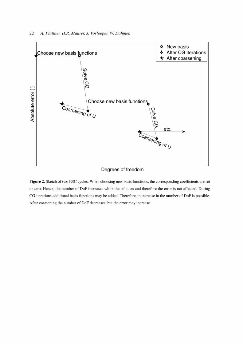
Figure 2 summarises the iterative procedure. The vertical axis indicates the true modelling error

and the horizontal axis indicates the degrees of freedom (DoF) (i.e., the number of scaling functions

and wavelets chosen). Here, the error is defined as the average absolute deviation between the true

function values (or a numerical reference solution calculated on a very fine mesh using a finite ele-

ment method) and their approximations determined on a fine sampling grid. The work/accuracy results

for such adaptive wavelet schemes refer to error bounds for the approximate solutions with respect to

the energy norm (in the present situation to the H1-norm, the sum of the square norm of the function

and the square norm of its gradient). In our subsequent tests we will, however, monitor averages of

pointwise errors as explained above which is not covered by the existing theory and may therefore

offer an interesting insight in this regard. The first horizontal segment of the process curve represents

the choice of new coefficients taken from the approximation of the residual R and the subsequent in-

clined segment indicates the accuracy improvement achieved during the CG iterations. The following

coarsening of vector U reduces the number of DoF, but may also result in a small increase of the

modelling error. The following segments represent the repeated cycles of

Estimate residual/choose new basis functions - Solve with CG - Coarsening (ESC).

A more extensive description of the algorithm is found in Appendix B and in Cohen et al. (2003).

Cohen et al. (2003) also includes the proofs of the following distinctive features of the algorithm:

(i) The final number of DoF required is optimal in the sense that it scales linearly with the theoret-

ical minimum number of DoF for a given accuracy (in the energy norm, as described above).

(ii) Memory consumption scales linearly with the final number of DoF. Hence, the sparsity of the

system matrix in equation 1 remains constant.

(iii) The number of scalar operations (i.e. scalar multiplications, including sorting) involved in the

algorithm scales linearly with the final number of DoF. Hence, computation time also scales linearly

with the final number of DoF.


2.4 A simple example

The functionality of the algorithm is demonstrated using a simple 1-D Laplace problem with zero

boundary conditions:

∆u(x) = f(x), (10)

where the function f(x) is chosen such that the solution should be

u(x) = (x2 sin(7πx)− 1)(x− 1)x. (11)

The left column panels in Figure 3 indicate the wavelets chosen within each iteration, whereas the right

column panels show the true (solid line) and approximated (dashed line) solutions. After iteration 2,

the true solution is roughly approximated and after 4 iterations the accuracy is already quite good.

Further iterations still improve the accuracy, but the associated error plot in Figure 4 indicates that the

absolute error begins to flatten out. This is due to the reduction of the error by a constant factor: if an

error of ε is reached, the error after the next iteration is at most βε for some fixed β ∈ (0, 1), which

may lead to insignificant improvements, if ε is already small.

Note that areas, where the solution shows almost linear behaviour, require a small number of

wavelet basis functions, whereas highly non-linear areas lead to a larger number of wavelet basis

functions (Figure 3). This effective compression is caused by the vanishing moments of the wavelet

basis.

3 NUMERICAL PERFORMANCE TESTS

We have applied our adaptive wavelet algorithm to a 3-D geoelectric problem on a rectangular prism

domain with Neumann boundary conditions on the surface boundary and mixed type boundary con-

ditions along the artificial ground boundaries. Furthermore, singularity removal was applied, that is,

equation 3 is solved.

The algorithm is expected to perform best when the structural complexity of the conductivity

distribution in the modelling domain is low. With increasing subsurface complexity, the performance

may degrade in terms of number of DoF. In fact, adaptivity shows the best performance when it is

applied in order to capture isolated features using only a small number of DoF. Conductivities that

exhibit rapid spatial variations across the domain require a fine mesh everywhere, which leads to an

almost uniform refinement.

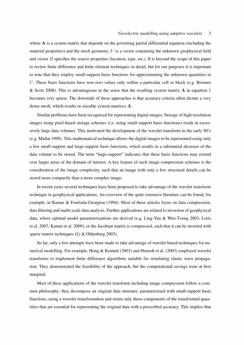
To investigate the behaviour of the algorithm, we have constructed three models of increasing

complexity. The first model consists of a homogeneous background conductivity (0.01 S/m) with a

single prismatic anomaly (0.1 S/m, Fig. 5a). The second model comprises six prismatic anomalies


of different sizes and shapes (Fig. 5b). Conductivities lie between 0.001 and 1 S/m. The third model

includes 343 equally sized blocks of stochastically distributed conductivities between 0.003 and 0.08

equally distributed in a homogeneous background medium (Fig. 5c). For all computations we con-

sidered a single current injection point located at (30,15,0) (indicated by the arrows in Figures 5a

to 5c).

In order to assess the performance of the adaptive wavelet algorithm and to show improvements

compared to widely used algorithms in the geophysical community, we additionally computed the

response of the three models in Figure 5 using the non-adaptive finite element code B2009 as de-

scribed in Blome et al. (2009). This finite element code is representative of the current state-of-the-art

in geoelectric modelling. It employs unstructured meshes and a direct matrix solver. To make the re-

sults more comparable with the adaptive wavelet algorithm, we substituted the direct matrix solver of

Blome et al. (2009) with a conjugate gradient solver using SSOR preconditioning (as is used in Spitzer

1995, for the finite difference method). For this type of problems, direct and CG solvers provide a sim-

ilar accuracy, when sufficient iterations are performed. Reference solutions were computed with the

B2009 algorithm using a very large number of elements (1.5 million DoF). The modelling error was

determined by interpolating the adaptive wavelet algorithm solution on the fine mesh of the reference

solution and computing the average absolute deviation with respect to the reference solution.

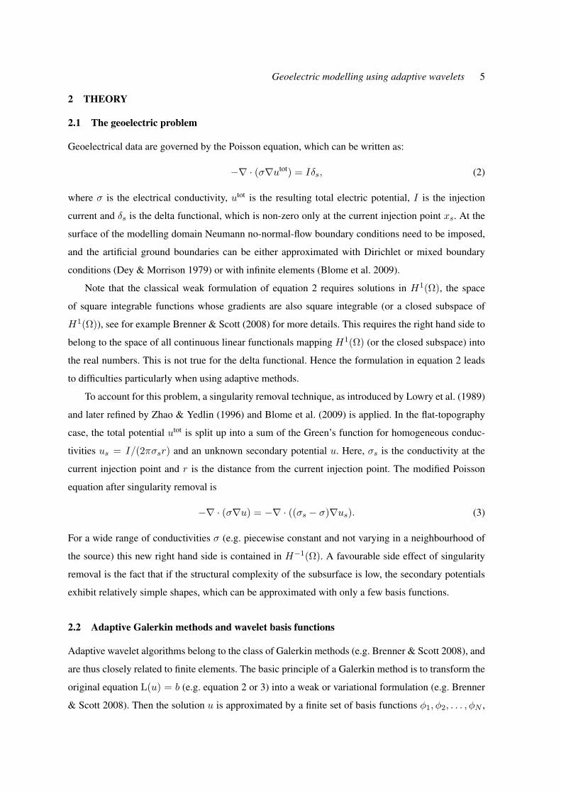
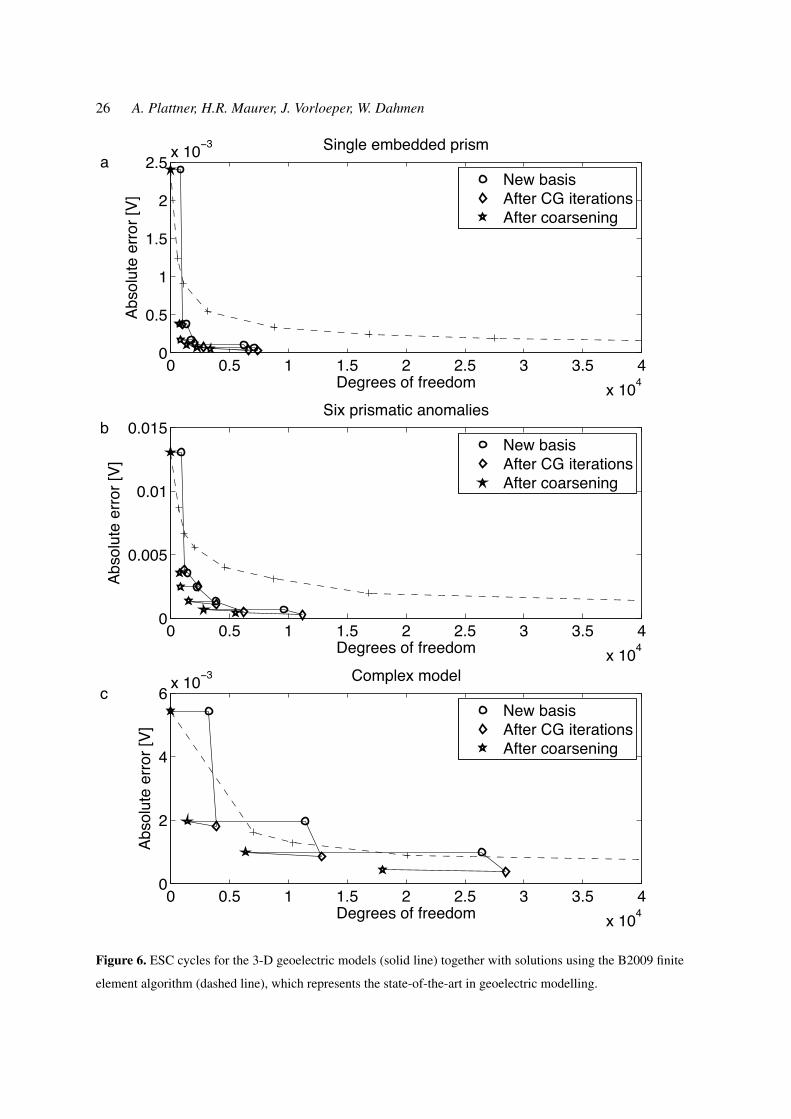
Figure 6 depicts the ESC cycles for the computations with the 3 models shown in Figure 5. Ad-

ditionally, the absolute errors of the B2009 algorithm are plotted as a function of the number of DoF.

CG iterations were carried out for the B2009 finite element algorithm until the CG residual reached

10−9, which is well below the actual modelling error. As expected, the performance of the adaptive

wavelet algorithm is excellent for the simple single embedded prism model (Fig. 6a). After only 3

ESC cycles the absolute error is at about 10−4, which is well below the error of the B2009 solution

with a comparable number of DoF. To achieve the same accuracy with the B2009 algorithm, roughly

twenty times more DoF would be required. Similar results were also obtained for the model with six

prismatic anomalies (Fig. 6b). For the most complex model (Fig. 6c) the performance of the adaptive

wavelet algorithm in terms of number of degrees of freedom degrades (as expected) and becomes

comparable to the B2009 finite element algorithm. Nevertheless, the adaptive method guarantees a

desired accuracy. If even more complex models would be considered, the performance of the adaptive

wavelet algorithm may further degrade during the first ESC cycles. In such situations homogenisation

or other upscaling techniques may be required.

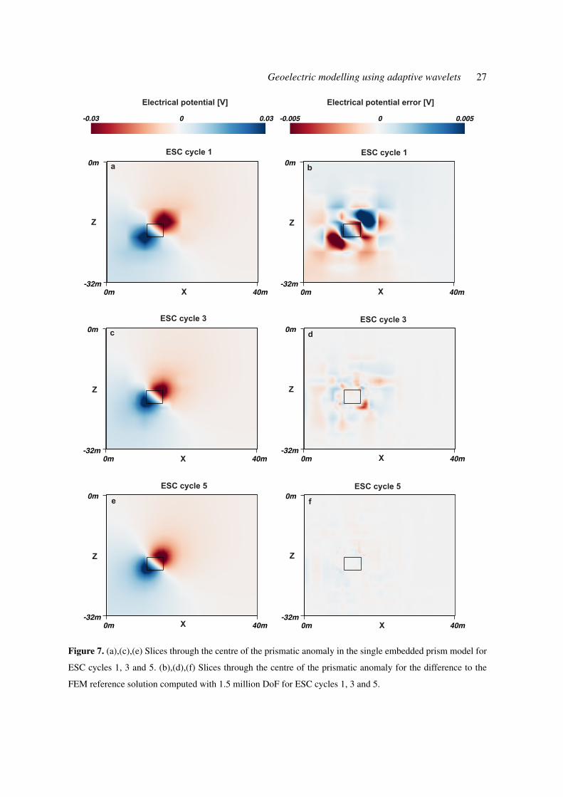
Besides this overall measure of accuracy (vertical axis in Figure 6), it is also instructive to observe

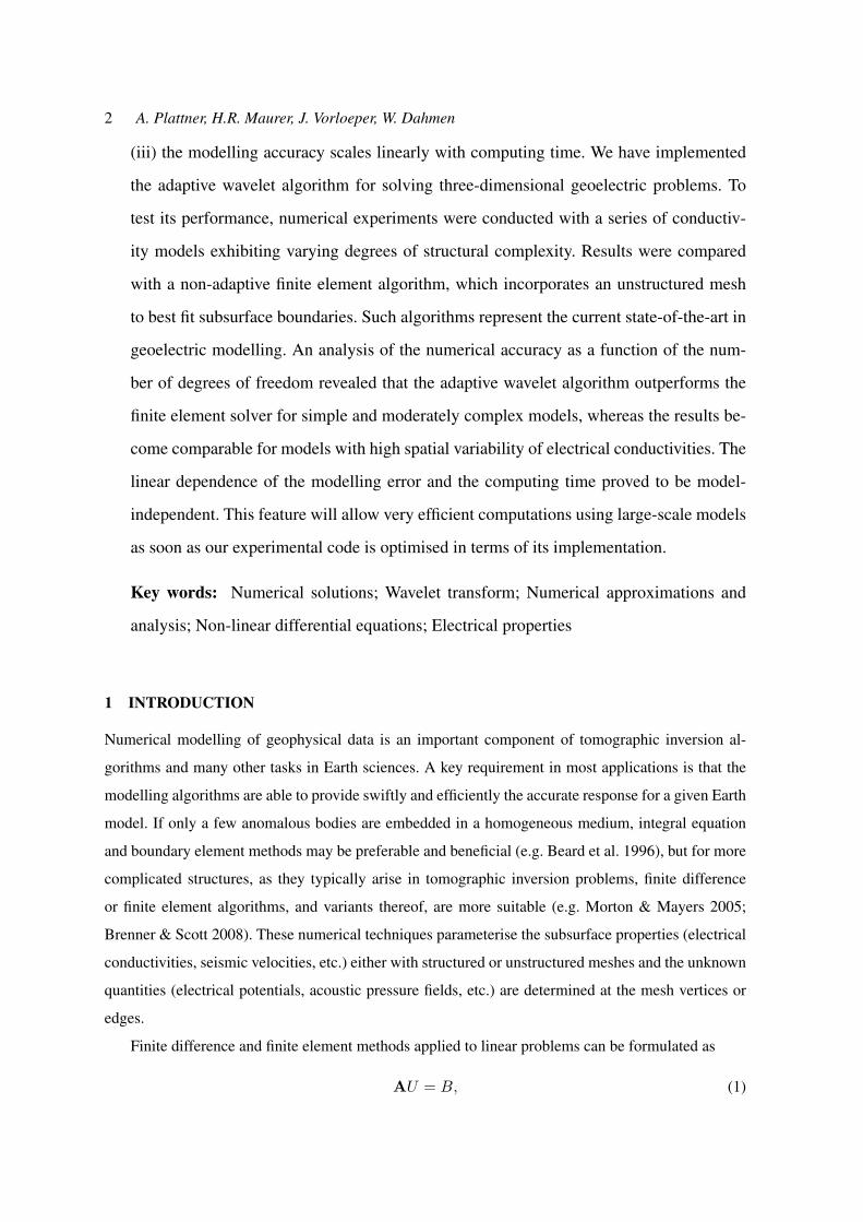
how the errors are distributed within the modelling domain. For that purpose we plotted slices through

the adaptive wavelet solutions (only the secondary potentials arising from the anomalous prism are


displayed) using the single prismatic anomaly model after completion of ESC cycles 1, 3 and 5 (Fig. 7).

Additionally, the corresponding differences to the reference solution are displayed. After the first

cycle, the solution is rather blocky, since it only considers scaling functions and low-level wavelets.

Nevertheless, it already captures the most important features of the bipolar secondary field created by

the prismatic anomaly. After ESC cycle 3, the solution improves significantly, and after ESC cycle 5

the relative errors become negligibly small.

As seen for the simple 1-D example in Figure 3, an excellent approximation of the solution is

already achieved with a few low-level wavelet basis functions in areas where the solution shows almost

linear behaviour (away from the conductivity contrasts). Close to the contrast, a number of higher-level

wavelet basis functions is required in order to accurately represent the solution.

Results in Figure 6 demonstrate the memory efficiency of the adaptive wavelet algorithm. That

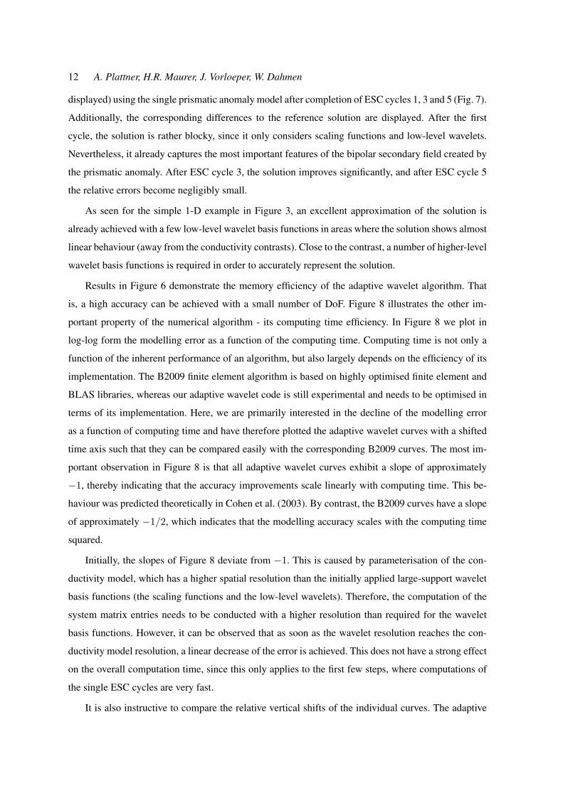
is, a high accuracy can be achieved with a small number of DoF. Figure 8 illustrates the other im-

portant property of the numerical algorithm - its computing time efficiency. In Figure 8 we plot in

log-log form the modelling error as a function of the computing time. Computing time is not only a

function of the inherent performance of an algorithm, but also largely depends on the efficiency of its

implementation. The B2009 finite element algorithm is based on highly optimised finite element and

BLAS libraries, whereas our adaptive wavelet code is still experimental and needs to be optimised in

terms of its implementation. Here, we are primarily interested in the decline of the modelling error

as a function of computing time and have therefore plotted the adaptive wavelet curves with a shifted

time axis such that they can be compared easily with the corresponding B2009 curves. The most im-

portant observation in Figure 8 is that all adaptive wavelet curves exhibit a slope of approximately

−1, thereby indicating that the accuracy improvements scale linearly with computing time. This be-

haviour was predicted theoretically in Cohen et al. (2003). By contrast, the B2009 curves have a slope

of approximately −1/2, which indicates that the modelling accuracy scales with the computing time

squared.

Initially, the slopes of Figure 8 deviate from −1. This is caused by parameterisation of the con-

ductivity model, which has a higher spatial resolution than the initially applied large-support wavelet

basis functions (the scaling functions and the low-level wavelets). Therefore, the computation of the

system matrix entries needs to be conducted with a higher resolution than required for the wavelet

basis functions. However, it can be observed that as soon as the wavelet resolution reaches the con-

ductivity model resolution, a linear decrease of the error is achieved. This does not have a strong effect

on the overall computation time, since this only applies to the first few steps, where computations of

the single ESC cycles are very fast.

It is also instructive to compare the relative vertical shifts of the individual curves. The adaptive


wavelet curves for the six prismatic anomalies model and the complex model lie on top of each other,

whereas the six prismatic anomalies curve for the B2009 algorithm lies well above the corresponding

complex model curve. This is most likely the result of the optimal preconditioning in the wavelet ba-

sis. The computational time of the adaptive wavelet algorithm does not depend on the magnitudes of

the contrasts but only on their geometrical distribution and hence the number of wavelets needed to

approximate the solution. In contrast, the non-adaptive B2009 computation time does not so much de-

pend on the geometry of the conductivity contrasts but mostly on their magnitudes, since this strongly

affects the condition number of the system of equations in equation 1. Hence the adaptive wavelet

algorithm is highly efficient, when the model complexity is low. Although the adaptive wavelet algo-

rithm shows a decrease in efficiency in terms of number of DoF when the models are more complex, its

slope of −1 still leads to superior performance compared to the B2009 method for higher accuracies.

4 DISCUSSION AND CONCLUSIONS

Using the example of 3-D geoelectric forward modelling we have demonstrated the capabilities and

limitations of adaptive wavelet algorithms, a novel technique that was proposed recently in the math-

ematical literature. To the best of our knowledge this is the first application of such techniques to a

geophysical problem. From our calculations we observe that

(i) the adaptive wavelet algorithm together with singularity removal is a powerful method for geo-

electric modelling

(ii) the error convergence rate is also good in the discrete L1-norm, which has not yet been covered

by the theory

(iii) the performance in terms of memory consumption and time-versus-error rate is superior to the

common methods currently applied in geoelectric modelling

(iv) general features of adaptive methods offer scope for further developments

Future research should focus on an optimised implementation of adaptive wavelet algorithms.

During the past few decades, probably a 1000 person years or even more have been dedicated to the

optimisation of finite element codes, while wavelet codes are still in an experimental stage and thus far

away from optimality. Fully exploiting the memory and computing time efficiency of adaptive wavelet

solvers will undoubtedly lead to substantial improvements in geophysical modelling.

This is particularly good news for those concerned with the challenging seismic modelling prob-

lem. With the increasing popularity of seismic waveform inversions, there is an urgent need for effi-

cient modelling algorithms. Conceptually, adaptive wavelet algorithms are well suited for acoustic and

elastic waveform modelling problems, but care should be taken with the choice of the right hand side


in equation 2 (source term), which needs to be at least square integrable. This may require application

of singularity removal techniques to the governing seismic differential equations.

ACKNOWLEDGMENTS

We thank Christoph Schwab for the initial suggestion of using adaptive wavelets for the geoelectric

problem. Furthermore we thank Stewart Greenhalgh and Andrew Jackson for their helpful comments

that improved the quality of the paper. Special thanks to Mark Blome for providing his finite element

implementation and for all his help with the calculations. This work was supported in part by the

Leibniz Program of the German Research Foundation and the Swiss National Foundation.

REFERENCES

Barinka, A., Barsch, T., Charton, P., Cohen, A., Dahlke, S., Dahmen, W., & Urban, K., 2001. Adaptive

wavelet schemes for elliptic problems implementation and numerical experiments, SIAM Journal on Scientific

Computing, 23(3), 910–939.

Beard, L., Hohmann, G., & Tripp, A., 1996. Fast resistivity IP inversion using a low-contrast approximation,

Geophysics, 61(1), 169–179.

Binev, P. & DeVore, R., 2004. Fast computation in adaptive tree approximation, Numerische Mathematik,

97(2), 193–217.

Binev, P., Dahmen, W., & DeVore, R., 2004. Adaptive finite element methods with convergence rates, Nu-

merische Mathematik, 97(2), 219–268.

Blome, M., Maurer, H. R., & Schmidt, K., 2009. Advances in three-dimensional geoelectric forward solver

techniques, Geophysical Journal International, 176(3), 740–752.

Brenner, S. C. & Scott, L. R., 2008. The Mathematical Theory of Finite Element Methods, Springer Berlin /

Heidelberg.

Cascon, J. M., Kreuzer, C., Nochetto, R. H., & Siebert, K. G., 2008. Quasi-optimal convergence rate for an

adaptive finite element method, SIAM Journal on Numerical Analysis, 46(5), 2524–2550.

Cohen, A. & Masson, R., 1999. Wavelet methods for second-order elliptic problems, preconditioning, and

adaptivity, Siam Journal on Scientific computing, 21(3), 1006–1026.

Cohen, A., Dahmen, W., & Devore, R., 2001. Adaptive wavelet methods for elliptic operator equations:

Convergence rates, Mathematics of Computation, 70(233), 27–75.

Cohen, A., Dahmen, W., & DeVore, R., 2003. Adaptive wavelet schemes for nonlinear variational problems,

SIAM Journal on Numerical Analysis, 41(5), 1785–1823.

Cohen, A., Daubechies, I., & Feauveau, J., 1992. Biorthogonal bases of compactly supported wavelets, Com-

munications on Pure and Applied Mathematics, 45(5), 485–560.

Cohen, A., Dahmen, W., & DeVore, R., 2002. Adaptive wavelet methods II - Beyond the elliptic case, Foun-

dations of Computational Mathematics, 2(3), 203–245.


Cohen, A., Dahmen, W., & Devore, R., 2003. Sparse evaluation of compositions of functions using multiscale

expansions, SIAM Journal on Mathematical Analysis, 35(2), 279–303.

Dahlke, S., Dahmen, W., Hochmuth, R., & Schneider, R., 1997. Stable multiscale bases and local error esti-

mation for elliptic problems, Applied Numerical Mathematics, 23(1), 21–47.

Dahmen, W., 2003. Multiscale and wavelet methods for operator equations, in Multiscale Problems and Meth-

ods in Numerical Simulations, vol. 1825 of Lecture Notes in Mathematics, pp. 31–96, CIME, Springer-

Verlag Berlin, Heidelberger Platz 3, D-14197 Berlin, Germany, CIME Summer School on Multiscale Prob-

lems and Methods in Numerical Simulations, Martina Franca, Italy, Sep 09-15, 2001.

Dahmen, W. & Schneider, R., 1999. Composite wavelet bases for operator equations, Mathematics of Compu-

tation, 68(228), 1533–1567.

Dahmen, W., Kunoth, A., & Urban, K., 1999. Biorthogonal spline wavelets on the interval - Stability and

moment conditions, Applied and Computational Harmonic Analysis, 6(2), 132–196.

Dahmen, W., Schneider, R., & Xu, Y., 2000. Nonlinear functionals of wavelet expansions - adaptive recon-

struction and fast evaluation, Numerische Mathematik, 86(1), 49–101.

Dey, A. & Morrison, H. F., 1979. Resistivity modeling for arbitrarily shaped 3-dimensional structures, Geo-

physics, 44(4), 753–780.

Gantumur, T., Harbrecht, H., & Stevenson, R., 2007. An optimal adaptive wavelet method without coarsening

of the iterands, Mathematics of Computation, 76(258), 615–629.

Glowinski, R., Lawton, W., Ravachol, M., & Tenenbaum, E., 1990. Wavelet solutions of linear and nonlin-

ear elliptic, parabolic and hyperbolic problems in one space dimension, in Computing methods in applied

sciences and engineering, pp. 55–120, SIAM.

Hong, T. & Kennett, B., 2003. Modelling of seismic waves in heterogeneous media using a wavelet-based

method: application to fault and subduction zones, Geophysical Journal International, 154(2), 483–498.

Hustedt, B., Operto, S., & Virieux, J., 2003. A multi-level direct-iterative solver for seismic wave propagation

modelling: space and wavelet approaches, Geophysical Journal International, 155(3), 953–980.

Jaffard, S., 1992. Wavelet methods for fast resolution of elliptic problems, SIAM Journal on Numerical Anal-

ysis, 29(4), 965–986.

Jiang, Y.-c. & Liu, Y., 2008. Adaptive Wavelet Solution to the Stokes Problem, Acta Mathematicae Applicatae

Sinica-English Series, 24(4), 613–626.

Kamm, J., Becken, M., & Yaramanci, U., 2009. Inversion of magnetic resonance sounding with wavelet basis

functions, in 15th European Meeting of Environmental and Engineering Geophysics.

Kumar, P. & Foufoula-Georgiou, E., 1994. Wavelets in Geophysics, Volume 4 (Wavelet Analysis and Its Appli-

cations), Academic Press.

Li, Y. & Oldenburg, D., 2003. Fast inversion of large-scale magnetic data using wavelet transforms and a

logarithmic barrier method, Geophysical Journal International, 152(2), 251–265.

Ling-Yun, C. & Wen-Tzong, L., 2003. Multiresolution parameterization for geophysical inverse problems,

Geophysics, 68(1), 199–209.


Loris, I., Nolet, G., Daubechies, I., & Dahlen, F. A., 2007. Tomographic inversion using l(1)-norm regulariza-

tion of wavelet coefficients, Geophysical Journal International, 170(1), 359–370.

Lowry, T., Allen, M. B., & Shive, P. N., 1989. Singularity removal - a refinement of resistivity modeling

techniques, Geophysics, 54(6), 766–774.

Maday, Y., Perrier, V., & Ravel, J., 1991. Dynamic adaptivity using wavelets basis for the approximation

of partial-differential equations, Comptes rendus de l’Academie des sciences serie I-mathematique, 312(5),

405–410.

Mallat, S., 1998. A wavelet tour of signal processing., San Diego, CA: Academic Press.

Morton, K. W. & Mayers, D. F., 2005. Numerical Solution of Partial Differential Equations, An Introduction,

Cambridge University Press.

Shewchuk, J. R., 1994. An introduction to the conjugate gradient method without the agonizing pain,

ftp://warp.cs.cmu.edu.

Spitzer, K., 1995. A 3-d finite difference algorithm for dc resistivity modelling using conjugate-gradient

methods, Geophysical Journal International, 123(3), 903–914.

Stevenson, R., 2003. On the compressibility of operators in wavelet coordinates, SIAM Journal on Mathemat-

ical Analysis, 35(5), 1110–1132.

Zhao, S. & Yedlin, M., 1996. Some refinements on the finite-difference method for 3-D dc resistivity modeling,

Geophysics, 61(5), 1301–1307.

APPENDIX A: WAVELETS

A1 More on one-dimensional wavelet basis functions

The one-dimensional scaling functions and wavelets considered in this appendix are confined to pow-

ers of the unit interval [0, 1], but extensions to other intervals can be achieved by shifting and dilation.

The wavelet basis functions on the inside of the interval are described with equations 5 and 6 in sec-

tion 2.2. At the boundaries 0 and 1, the following functions are used

ϕl,0(x) =

23l2 (2−l − x) if 0 ≤ x ≤ 2−l

0 elsewhere(A.1)

and

ϕl,2l(x) =

23l2 (x+ 2−l − 1) if 1− 2−l ≤ x ≤ 1

0 elsewhere,(A.2)

for the scaling functions and

ψl,1 =1√2

(− 34ϕl+1,0 +

916ϕl+1,1+

− 18ϕl+1,2 −

116ϕl+1,3)

(A.3)


and

ψl,2l =1√2

(− 116ϕl+1,2l+1−3 −

18ϕl+1,2l+1−2+

+916ϕl+1,2l+1−1 −

34ϕl+1,2l+1),

(A.4)

for the wavelets (Cohen et al. 1992; Dahmen et al. 1999).

V 1Dl := span(ϕl,k | 0 ≤ k ≤ 2l) is the vector space of all possible linear combinations of the

scaling functions at level l and W 1Dl := span(ψl,k | 1 ≤ k ≤ 2l) is the vector space of all possible

linear combinations of the wavelets at level l. They are related as follows:

. . . ⊂ V 1D2 ⊂ V 1D

3 ⊂ V 1D4 ⊂ . . . , (A.5)

W 1Dl ⊂ V 1D

l+1 and V 1Dl+1 = V 1D

l ⊕W 1Dl . (A.6)

These piecewise linear wavelets have the advantage that they are very simple to handle within in-

tegrals. Furthermore, they are not orthogonal (not required for our algorithm) but biorthogonal (Cohen

et al. 1992).

A2 Wavelet basis functions in two and more dimensions

Tensor product constructions can be used for creating higher-dimensional wavelet basis functions

(Dahmen & Schneider 1999). The tensor product of a function f(x) with a function g(y) is defined as

(f ⊗ g)(x, y) := f(x)g(y). (A.7)

The tensor product of two function spaces V and W is the linear span of all tensor products of func-

tions in V with functions in W . Note that in general f ⊗ g 6= g ⊗ f . We use this definition to

create wavelet basis functions in two dimensions. Two-dimensional scaling functions are identified

with three parameters: level l, shift in x-direction kx and shift in y-direction ky. The scaling functions

ϕl,kx,ky(x, y) are defined as

ϕl,kx,ky(x, y) :=(ϕl,kx ⊗ ϕl,ky)(x, y)

=ϕl,kx(x)ϕl,ky(y).(A.8)

We denote the two-dimensional scaling functions by V 2Dl := span(ϕl,kx,ky | 0 ≤ kx ≤ 2l and 0 ≤

ky ≤ 2l). Wavelets in two dimensions are the complement of V 2Dl in V 2D

l+1 . Using V 2Dl = V 1D

l ⊗V 1Dl

we get

V 2Dl+1 =V 1D

l+1 ⊗ V 1Dl+1 = (V 1D

l ⊕W 1Dl )⊗ (V 1D

l ⊕W 1Dl )

=(V 1Dl ⊗ V 1D

l )⊕ (V 1Dl ⊗W 1D

l )⊕

⊕ (W 1Dl ⊗ V 1D

l )⊕ (W 1Dl ⊗W 1D

l ).

(A.9)


Hence

W 2Dl =(V 1D

l ⊗W 1Dl )⊕ (W 1D

l ⊗ V 1Dl )⊕

⊕ (W 1Dl ⊗W 1D

l ).(A.10)

Therefore the wavelets in two dimensions consist of functions of the shapeϕl,kx(x)ψl,ky(y), ψl,kx(x)ϕl,ky(y)

and ψl,kx(x)ψl,ky(y). Wavelet bases in higher dimensions can be constructed accordingly.

APPENDIX B: THE ADAPTIVE WAVELET ALGORITHM

In this Appendix, we give an overview of the implementation of our algorithm that largely follows

Cohen et al. (2003). For more details, we therefore refer to the Cohen et al. (2003) paper and the

references contained therein. For practical reasons, we have replaced the damped Richardson iteration

in Cohen et al. (2003) by a CG method.

The algorithm depends on a set of parameters, which we will describe briefly. The coefficient β

estimates the ratio of the absolute error between a given approximation U of the solution Utotal and

the estimated residual of U depending on the underlying problem and the chosen iterative solver (here

CG). C∗ controls the Astree-norms of the resulting vector after the coarsening, where Astree-norm is a

measure for the approximability of a vector by small trees. The parameter γ, which plays an important

role in the adaptive operator approximation describes the wavelet compressibility of the operator.

The parameter ρ ∈ (0, 1) and the summable sequence of parameters ωk∞k=0 can be freely chosen.

They influence the computation time and the memory consumption but do not influence the linear

work/accuracy rate. Note that these parameters are adapted to the damped Richardson iteration and no

mathematical proof exists for the application of the CG method. In our case, we set β = 100, C∗ =

2, γ = 7, ρ = 0.95, ωk = 0.9k.

Sets of wavelet basis functions (which in this algorithm always form a tree) are denoted with Λ.

We write Λn for sets of newly acquired functions, Λn for the sets after the CG-iterations and Λn for

the coarsened sets. The associated vectors of coefficients are denoted by B for the right hand side, U

for the solution and R for the approximation of the residual, where the index set is indicated in the

subscript.

Algorithm AdaptiveSolve(ε)

Input: desired accuracy

Output: Optimal set of functions Λopt, solution UΛopt

(∗Main algorithm ∗)

1. Calculate the wavelet expansion of the right hand side∑

λ∈Λfullbλφλ

2. Set BΛfull = (bλ)λ∈Λfull


3. Set n = 0; Λ0 = ∅; UΛ0= 0

4. Set ε0 = ‖BΛfull‖25. while εn > ε

6. do Set n = n+ 1

7. [Λn, RΛn] = Estimate-

8. Residual(Λn−1, UΛn−1, BΛfull , ω0εn−1)

9. [Λn, UΛn ] = SolveCG(Λn, UΛn−1, RΛn

, εn−1)

10. [Λn, UΛn] = Coarse(UΛn , εn−1C

∗/(2 + 2C∗))

11. Set εn = εn−1/2

12. return Λopt = Λn;UΛopt = UΛn

The three steps EstimateResidual, SolveCG and Coarse correspond to the ESC steps described in

section 2.3. The subroutine EstimateResidual is defined as

Algorithm EstimateResidual(Λn−1, UΛn−1, BΛfull , εn−1)

Input: Set of functions, solution, right hand side, desired accuracy

Output: Set of functions Λn, Approximation of the residual RΛn,

(∗ Approximates the residual ∗)

1. [Λ1, V ] = ApplyOperator(UΛn−1, 0.5ω0εn−1)

2. [Λ2,W ] = Coarse(BΛfull , 0.5ω0εn−1)

3. return RΛn:= V −W and Λn := Those functions in Λ1 ∪ Λ2, for which V −W has nonzero

entries

In this subroutine the function ApplyOperator, which approximates the application of the operator to

the current solution with the given accuracy is the core ingredient of the adaptive wavelet algorithm.

Since the application of the operator cannot be computed (this would result in a multiplication of a

rectangular infinite matrix with a finite vector), it needs to be approximated. The approximation is

conducted by first setting up a tree of wavelet basis functions for which the coefficients will approx-

imate the application with the desired accuracy (see Cohen et al. 2003, theorem 3.4 and the related

construction of the tree), then calculating the coefficients using the fast top-down evaluation scheme

described in Dahmen et al. (2000). Before the approximation is calculated, a diagonal preconditioner

di = 1/√aii is applied, where aii are the diagonal entries of the system matrix A in equation 8.

This ensures an optimal condition number (Cohen & Masson 1999). Here, “optimality” indicates that

the condition number of the preconditioned system matrix is bounded for all detail levels. Hence all

solutions using a CG algorithm on a fixed basis can be calculated up to a given accuracy using a fixed


(small) number of CG iterations. Other possibilities of optimal preconditioning can be found in Cohen

& Masson (1999).

The subroutine SolveCG is set up as

Algorithm SolveCG(Λn, UΛn−1, RΛn

, εn−1)

Input: Set of functions, previous solution, approximated residual of the previous solution, desired

accuracy

Output: Set of functions Λn, solution UΛn ,

(∗Modified conjugate gradient solver ∗)

1. Set k = 0; Λ0 = Λn;U0 = UΛn−1

2. Set P k = RΛn;Rk = −RΛn

3. while ωkρkεn−1 + ‖Rk‖2 > εn−1/((2 + 2C∗)β)

4. do Set k=k+1

5. [Λk, V ] = ApplyOperator(P k−1, 0.5ωkρkεn−1)

6. Uk = Uk−1 + (Rk−1·Rk−1)(Pk−1·V )

P k−1

7. Rk = Rk−1 + (Rk−1·Rk−1)(Pk−1·V )

V

8. P k = (Rk·Rk)(Rk−1·Rk−1)

P k−1 −Rk

9. return Λn = Λk;UΛn = Uk

This routine is a generic conjugate gradient solver (e.g. Shewchuk 1994), except that the application

of the operator restricted to Λn is replaced by the function ApplyOperator described above.

In the function Coarse an as large as possible number of coefficients is removed from the given

vector, such that the norm of the difference from the initial vector is smaller than a prescribed value

0.5ω0εn−1. Additionally, the tree structure is preserved. An exact description of this procedure can be

found in Binev & DeVore (2004).

Optimality is achieved by keeping the number of scalar operations linear with the number of

wavelet basis functions in the routines ApplyOperator and Coarse. Since the condition number of the

diagonally preconditioned operator in the wavelet basis is always smaller than cmax, the number of

iterations inside the SolveCG routine does not exceed a maximum number K if the basis does not

vary after the first few steps. Because each ESC cycle leads to an error reduction by a constant factor,

only a fixed maximum number of iterations is required to reach a given target accuracy. Therefore, the

number of total scalar operations scales linearly with the final number of degrees of freedom.


0 0.125 0.25 0.375 0.5 0.625 0.75 0.875 1

2

3

4

5Scaling functions for starting level l0 = 2

x

Leve

l

a

0 0.125 0.25 0.375 0.5 0.625 0.75 0.875 1

2

3

4

5

x

Leve

l l

Selection of wavelets on different levels l ≥ 2b

0 0.125 0.25 0.375 0.5 0.625 0.75 0.875 10

1FEM hat functions

x

FEM

hat

func

tion

valu

e

c

Figure 1. Examples of 1-D model parameterisations. (a) Scaling functions at level 2. (b) A selection of wavelets

on different levels with different positions. (c) FEM hat functions for an equivalent resolution as the wavelet

basis up to level 2. The dashed lines indicate the nodes of the hat functions. The finite elements are the intervals

between the dashed lines on the x-axis.


Degrees of freedom

Abso

lute

erro

r [ ]

Choose new basis functions

Solve CG

Coarsening of U

Choose new basis functions

Solve CG

Coarsening of U

etc.

New basisAfter CG iterationsAfter coarsening

Figure 2. Sketch of two ESC cycles. When choosing new basis functions, the corresponding coefficients are set

to zero. Hence, the number of DoF increases while the solution and therefore the error is not affected. During

CG-iterations additional basis functions may be added. Therefore an increase in the number of DoF is possible.

After coarsening the number of DoF decreases, but the error may increase.


0 0.25 0.5 0.75 1345678

Level

x

a

0 0.25 0.5 0.75 10

0.2

x

u(x)

b

0 0.25 0.5 0.75 1345678

Level

x

c

0 0.25 0.5 0.75 10

0.2

x

u(x)

d

0 0.25 0.5 0.75 1345678

Level

x

e

0 0.25 0.5 0.75 10

0.2

x

u(x)

f

0 0.25 0.5 0.75 1345678

Level

x

g

0 0.25 0.5 0.75 10

0.2

x

u(x)

h

Figure 3. (a),(c),(e),(g) The positions of the wavelets used for the ESC cycles 2,4,6 and 8 after coarsening. The

scaling functions are not displayed. (b),(d),(f),(h) show the adaptive wavelet solution after ESC cycles 2,4,6

and 8 (dashed line) compared to the analytic solution (solid line). Wherever rapid changes in the solution occur,

high-level wavelets are needed. In areas, where the analytic solution almost shows linear behaviour, only a small

number of wavelets is required.


0 50 100 150 200 250 3000

0.02

0.04

0.06

0.08

0.1

0.12

0.14

0.16

0.18

Degrees of freedom

Abso

lute

erro

r [ ]

New basisAfter CG iterationsAfter coarsening

Figure 4. ESC cycles for the simple 1-D example shown in Figure 3.


20m

0m

-32m

0m 0m

40m

20m -32m

0m 0m

0m

40m

20m

0m

-32m

0m 0m

40m

u

1.e-04

1.e-02

1.e+00

u

1.e-04

1.e-02

1.e+00

Sing

le e

mbe

dded

pris

mSi

x pr

ism

atic

ano

mal

ies

Com

plex

mod

el

Con

duct

ivity

[S/m

]C

ondu

ctiv

ity [S

/m]

Con

duct

ivity

[S/m

]

a

b

c

X

Y

Z

X

X

Z

Z

Y

Y

u

3.e-03

9.e-03

3.e-02

Figure 5. Conductivity models used to test the adaptive wavelet algorithm. The background conductivity is 0.01

S/m for each model. Source positions are indicated by arrows.


0 0.5 1 1.5 2 2.5 3 3.5 4x 104

0

0.5

1

1.5

2

2.5 x 10−3

Degrees of freedom

Abso

lute

erro

r [V]

Single embedded prism

aNew basisAfter CG iterationsAfter coarsening

0 0.5 1 1.5 2 2.5 3 3.5 4x 104

0

0.005

0.01

0.015

Degrees of freedom

Abso

lute

erro

r [V]

Six prismatic anomalies

bNew basisAfter CG iterationsAfter coarsening

0 0.5 1 1.5 2 2.5 3 3.5 4x 104

0

2

4

6 x 10−3

Degrees of freedom

Abso

lute

erro

r [V]

Complex model

cNew basisAfter CG iterationsAfter coarsening

Figure 6. ESC cycles for the 3-D geoelectric models (solid line) together with solutions using the B2009 finite

element algorithm (dashed line), which represents the state-of-the-art in geoelectric modelling.


40m 0m

0m

-32m

40m 0m

0m

-32m

40m 0m

0m

-32m

40m 0m

0m

-32m

40m 0m

0m

-32m

40m 0m

0m

-32m

-0.005 0 0.005-0.03 0 0.03

Electrical potential [V] Electrical potential error [V]

ESC cycle 1 ESC cycle 1

ESC cycle 3

ESC cycle 5

ESC cycle 3

ESC cycle 5

a b

c d

e f

Z Z

Z Z

Z Z

X X

X X

X X

Figure 7. (a),(c),(e) Slices through the centre of the prismatic anomaly in the single embedded prism model for

ESC cycles 1, 3 and 5. (b),(d),(f) Slices through the centre of the prismatic anomaly for the difference to the

FEM reference solution computed with 1.5 million DoF for ESC cycles 1, 3 and 5.


10 100 101 10210

10

10

10

Abso

lute

erro

r [V]

Runtime [s]

Wavelets, single embedded prismWavelets, six prismatic anomaliesWavelets, complex modelB2009, single embedded prismB2009, six prismatic anomaliesB2009, complex model

101 102 10 10

Figure 8. Error versus time slopes for the adaptive wavelet algorithm (red lines) and the B2009 finite element

algorithm (blue lines) for the three models Fig. 5a (circles), Fig. 5b (triangles) and Fig. 5c (stars).

Three-dimensional geoelectric modelling with optimal work - IGPM

Documents

Transcript of Three-dimensional geoelectric modelling with optimal work - IGPM