Three-Dimensional Computational Analysis of Transport ... · PDF fileThree-Dimensional...
205
Three-Dimensional Computational Analysis of Transport Phenomena in a PEM Fuel Cell by Torsten Berning Dipl.-Ing., RWTH Aachen, 1997 A Dissertation Submitted in Partial Ful…llment of the Requirements for the Degree of Doctor of Philosophy in the Department of Mechanical Engineering. We accept this dissertation as conforming to the required standard Dr. N. Djilali, Supervisor (Department of Mechanical Engineering) Dr. Z. Dong, Departmental Member (Department of Mechanical Engineering) Dr. S. Dost, Departmental Member (Department of Mechanical Engineering) Dr. F. Gebali, Outside Member (Department of Electrical Engineering) Dr. T. V. Nguyen, External Examiner (University of Kansas) c ° Torsten Berning, 2002 University of Victoria All rights reserved. This dissertation may not be reproduced in whole or in part, by photocopy or other means, without permission of the author.
Transcript of Three-Dimensional Computational Analysis of Transport ... · PDF fileThree-Dimensional...

Three-Dimensional Computational Analysis of TransportPhenomena in a PEM Fuel Cell
by
Torsten BerningDipl.-Ing., RWTH Aachen, 1997
A Dissertation Submitted in Partial Ful…llment of theRequirements for the Degree of
Doctor of Philosophy
in the Department of Mechanical Engineering.
We accept this dissertation as conformingto the required standard
Dr. N. Djilali, Supervisor (Department of Mechanical Engineering)
Dr. Z. Dong, Departmental Member (Department of Mechanical Engineering)
Dr. S. Dost, Departmental Member (Department of Mechanical Engineering)
Dr. F. Gebali, Outside Member (Department of Electrical Engineering)
Dr. T. V. Nguyen, External Examiner (University of Kansas)
c° Torsten Berning, 2002University of Victoria
All rights reserved. This dissertation may not be reproduced in whole or in part, byphotocopy or other means, without permission of the author.

Supervisor: Dr. N. Djilali
Abstract
Fuel cells are electrochemical devices that rely on the transport of reactants (oxygen
and hydrogen) and products (water and heat). These transport processes are cou-
pled with electrochemistry and further complicated by phase change, porous media
(gas di¤usion electrodes) and a complex geometry. This thesis presents a three-
dimensional, non-isothermal computational model of a proton exchange membrane
fuel cell (PEMFC). The model was developed to improve fundamental understand-
ing of transport phenomena in PEMFCs and to investigate the impact of various
operation parameters on performance. The model, which was implemented into a
Computational Fluid Dynamics code, accounts for all major transport phenomena,
including: water and proton transport through the membrane; electrochemical reac-
tion; transport of electrons; transport and phase change of water in the gas di¤usion
electrodes; temperature variation; di¤usion of multi-component gas mixtures in the
electrodes; pressure gradients; multi-component convective heat and mass transport
in the gas ‡ow channels.
Simulations employing the single-phase version of the model are performed for
a straight channel section of a complete cell including the anode and cathode ‡ow
channels. Base case simulations are presented and analyzed with a focus on the
physical insight and fundamental understanding a¤orded by the availability of de-
tailed distributions of reactant concentrations, current densities, temperature and
water ‡uxes. The results are consistent with available experimental observations and
ii

show that signi…cant temperature gradients exist within the cell, with temperature
di¤erences of several degrees Kelvin within the membrane-electrode-assembly. The
three-dimensional nature of the transport processes is particularly pronounced under
the collector plates land area, and has a major impact on the current distribution
and predicted limiting current density. A parametric study with the single-phase
computational model is also presented to investigate the e¤ect of various operating,
geometric and material parameters, including temperature, pressure, stoichiometric
‡ow ratio, porosity and thickness of the gas di¤usion layers, and the ratio between
the channel with and the land area.
The two-phase version of the computational model is used for a domain including a
cooling channel adjacent to the cell. Simulations are performed over a range of current
densities. The analysis reveals a complex interplay between several competing phase
change mechanisms in the gas di¤usion electrodes. Results show that the liquid
water saturation is below 0.1 inside both anode and cathode gas di¤usion layers.
For the anode side, saturation increases with increasing current density, whereas at
the cathode side saturation reaches a maximum at an intermediate current density
(¼ 1:1Amp=cm2) and decreases thereafter. The simulation show that a variety of
‡ow regimes for liquid water and vapour are present at di¤erent locations in the cell,
and these depend further on current density.
The PEMFC model presented in this thesis has a number of novel features that
enhance the physical realism of the simulations and provide insight, particularly in
heat and water management. The model should serve as a good foundation for future
development of a computationally based design and optimization method.
iii

Examiners:
Dr. N. Djilali, Supervisor (Department of Mechanical Engineering)
Dr. Z. Dong, Departmental Member (Department of Mechanical Engineering)
Dr. S. Dost, Departmental Member (Department of Mechanical Engineering)
Dr. F. Gebali, Outside Member (Department of Electrical Engineering)
Dr. T. V. Nguyen, External Examiner (University of Kansas)
iv

Table of Contents
Abstract ii
Table of Contents v
List of Figures ix
List of Tables xvi
Nomenclature xviii
Acknowledgements xxiv
1 Introduction 1
1.1 Background . . . . . . . . . . . . . . . . . . . . . . . . . . . . . . . . 1
1.2 Operation Principle of a PEM Fuel Cell . . . . . . . . . . . . . . . . . 3
1.3 Fuel Cell Components . . . . . . . . . . . . . . . . . . . . . . . . . . 4
1.3.1 Polymer Electrolyte Membrane . . . . . . . . . . . . . . . . . 4
1.3.2 Catalyst Layer . . . . . . . . . . . . . . . . . . . . . . . . . . 5
1.3.3 Gas-Di¤usion Electrodes . . . . . . . . . . . . . . . . . . . . . 6
1.3.4 Bipolar Plates . . . . . . . . . . . . . . . . . . . . . . . . . . . 6
v

1.4 Fuel Cell Thermodynamics . . . . . . . . . . . . . . . . . . . . . . . . 7
1.4.1 Free-Energy Change of a Chemical Reaction . . . . . . . . . . 7
1.4.2 From the Free-Energy Change to the Cell Potential: The Nernst
Equation . . . . . . . . . . . . . . . . . . . . . . . . . . . . . . 9
1.4.3 Fuel Cell Performance . . . . . . . . . . . . . . . . . . . . . . 14
1.4.4 Fuel Cell E¢ciencies . . . . . . . . . . . . . . . . . . . . . . . 17
1.5 Fuel Cell Modelling: A Literature Review . . . . . . . . . . . . . . . . 21
1.6 Thesis Goal . . . . . . . . . . . . . . . . . . . . . . . . . . . . . . . . 25
2 A Three-Dimensional, One-Phase Model of a PEM Fuel Cell 26
2.1 Introduction . . . . . . . . . . . . . . . . . . . . . . . . . . . . . . . . 26
2.2 Modelling Domain and Geometry . . . . . . . . . . . . . . . . . . . . 27
2.3 Assumptions . . . . . . . . . . . . . . . . . . . . . . . . . . . . . . . . 29
2.4 Modelling Equations . . . . . . . . . . . . . . . . . . . . . . . . . . . 30
2.4.1 Notation . . . . . . . . . . . . . . . . . . . . . . . . . . . . . . 30
2.4.2 Main Computational Domain . . . . . . . . . . . . . . . . . . 30
2.4.3 Computational Subdomain I . . . . . . . . . . . . . . . . . . . 37
2.4.4 Computational Subdomain II . . . . . . . . . . . . . . . . . . 40
2.4.5 Computational Subdomain III . . . . . . . . . . . . . . . . . . 41
2.4.6 Cell Potential . . . . . . . . . . . . . . . . . . . . . . . . . . . 41
2.5 Boundary Conditions . . . . . . . . . . . . . . . . . . . . . . . . . . . 43
2.5.1 Main Computational Domain . . . . . . . . . . . . . . . . . . 43
2.5.2 Computational Subdomain I . . . . . . . . . . . . . . . . . . . 45
2.5.3 Computational Subdomain II . . . . . . . . . . . . . . . . . . 45
2.5.4 Computational Subdomain III . . . . . . . . . . . . . . . . . . 46
vi

2.6 Computational Procedure . . . . . . . . . . . . . . . . . . . . . . . . 47
2.6.1 Discretization Method . . . . . . . . . . . . . . . . . . . . . . 47
2.6.2 Computational Grid . . . . . . . . . . . . . . . . . . . . . . . 50
2.7 Modelling Parameters . . . . . . . . . . . . . . . . . . . . . . . . . . . 51
2.8 Base Case Results . . . . . . . . . . . . . . . . . . . . . . . . . . . . . 56
2.8.1 Validation Comparisons . . . . . . . . . . . . . . . . . . . . . 56
2.8.2 Reactant Gas and Temperature Distribution Inside the Fuel Cell 60
2.8.3 Current Density Distribution . . . . . . . . . . . . . . . . . . 68
2.8.4 Liquid Water Flux and Potential Distribution in the Membrane 71
2.8.5 Grid Re…nement Study . . . . . . . . . . . . . . . . . . . . . . 76
2.8.6 Summary . . . . . . . . . . . . . . . . . . . . . . . . . . . . . 80
3 A Parametric Study Using the Single-Phase Model 81
3.1 Introduction . . . . . . . . . . . . . . . . . . . . . . . . . . . . . . . . 81
3.2 E¤ect of Temperature . . . . . . . . . . . . . . . . . . . . . . . . . . 83
3.3 E¤ect of Pressure . . . . . . . . . . . . . . . . . . . . . . . . . . . . . 90
3.4 E¤ect of Stoichiometric Flow Ratio . . . . . . . . . . . . . . . . . . . 96
3.5 E¤ect of Oxygen Enrichment . . . . . . . . . . . . . . . . . . . . . . . 99
3.6 E¤ect of GDL Porosity . . . . . . . . . . . . . . . . . . . . . . . . . . 101
3.7 E¤ect of GDL Thickness . . . . . . . . . . . . . . . . . . . . . . . . . 106
3.8 E¤ect of Channel-Width-to-Land-Area Ratio . . . . . . . . . . . . . . 110
3.9 Summary . . . . . . . . . . . . . . . . . . . . . . . . . . . . . . . . . 114
4 A Three-Dimensional, Two-Phase Model of a PEM Fuel Cell 115
4.1 Introduction . . . . . . . . . . . . . . . . . . . . . . . . . . . . . . . . 115
4.2 Modelling Domain and Geometry . . . . . . . . . . . . . . . . . . . . 117
vii

4.3 Assumptions . . . . . . . . . . . . . . . . . . . . . . . . . . . . . . . . 118
4.4 Modelling Equations . . . . . . . . . . . . . . . . . . . . . . . . . . . 119
4.4.1 Main Computational Domain . . . . . . . . . . . . . . . . . . 120
4.4.2 Computational Subdomain I . . . . . . . . . . . . . . . . . . . 132
4.5 Boundary Conditions . . . . . . . . . . . . . . . . . . . . . . . . . . . 132
4.6 Modelling Parameters . . . . . . . . . . . . . . . . . . . . . . . . . . . 132
4.7 Results . . . . . . . . . . . . . . . . . . . . . . . . . . . . . . . . . . . 135
4.7.1 Basic Considerations . . . . . . . . . . . . . . . . . . . . . . . 135
4.7.2 Base Case Results . . . . . . . . . . . . . . . . . . . . . . . . . 138
4.8 Summary . . . . . . . . . . . . . . . . . . . . . . . . . . . . . . . . . 157
5 Conclusions and Outlook 160
5.1 Conclusions . . . . . . . . . . . . . . . . . . . . . . . . . . . . . . . . 160
5.2 Contributions . . . . . . . . . . . . . . . . . . . . . . . . . . . . . . . 161
5.3 Outlook . . . . . . . . . . . . . . . . . . . . . . . . . . . . . . . . . . 162
A On Multicomponent Di¤usion 164
B Comparison between the Schlögl Equation and the Nernst-Planck
Equation 169
C The Dependence of the Hydraulic Permeability of the GDL on the
Porosity 173
References 175
viii

List of Figures
1.1 Operating scheme of a PEM Fuel Cell. . . . . . . . . . . . . . . . . . 3
1.2 Open system boundaries for thermodynamic considerations. . . . . . 9
1.3 Typical polarization curve of a PEM Fuel Cell and predominant loss
mechanisms in various current density regions. . . . . . . . . . . . . . 14
1.4 Comparison between the maximum theoretical e¢ciencies of a fuel cell
at standard pressure with a Carnot Cycle at a lower temperature of
Tc = 50 ±C : . . . . . . . . . . . . . . . . . . . . . . . . . . . . . . . . 18
2.1 The modeling domain used for the three-dimensional model. . . . . . 28
2.2 Flow diagram of the solution procedure used. . . . . . . . . . . . . . 48
2.3 Numerical grid of the main computational domain. . . . . . . . . . . 50
2.4 Comparison of polarization curves and power density curves between
the 3D modelling results and experiments. . . . . . . . . . . . . . . . 58
2.5 The break-up of di¤erent loss mechanisms at base case conditions. . . 59
2.6 Reactant gas distribution in the anode channel and GDL (upper) and
cathode channel and GDL (lower) at a nominal current density of
0:4A = cm2 at base case conditions. . . . . . . . . . . . . . . . . . . . 64
ix

2.7 Reactant gas distribution in the anode channel and GDL (upper) and
cathode channel and GDL (lower) at a nominal current density of
1:4A = cm2 at base case conditions. . . . . . . . . . . . . . . . . . . . 65
2.8 Molar oxygen concentration at the catalyst layer for six di¤erent cur-
rent densities: 0:2A = cm2 (upper left), 0:4A = cm2 (upper right), 0:6A = cm2
(centre left), 0:8A = cm2 (centre right), 1:0A = cm2 (lower left) and
1:2A = cm2 (lower right). . . . . . . . . . . . . . . . . . . . . . . . . . 66
2.9 Temperature distribution inside the fuel cell at base case conditions
for two di¤erent nominal current densities: 0:4A = cm2 (upper) and
1:4A = cm2 (lower). . . . . . . . . . . . . . . . . . . . . . . . . . . . . 67
2.10 Dimensionless current density distribution i=iave at the cathode side
catalyst layer for three di¤erent nominal current densities: 0:2A = cm2
(upper), 0:8A = cm2 (middle) and 1:4A = cm2 (lower). . . . . . . . . 69
2.11 Fraction of the total current generated under the channel area as op-
posed to the land area. . . . . . . . . . . . . . . . . . . . . . . . . . . 70
2.12 Liquid water velocity …eld (vectors) and potential distribution (con-
tours) inside the membrane at base case conditions for three di¤er-
ent current densities: 0:1A = cm2 (upper), 0:2A = cm2 (middle) and
1:2A = cm2 (lower). The vector scale is 200 cm = (m = s), 20 cm = (m = s),
and 2 cm = (m = s), respectively. . . . . . . . . . . . . . . . . . . . . . . 72
2.13 Comparison of values for the net drag coe¢cient ® for two di¤erent
values of the electrokinetic permeability of the membrane. . . . . . . 75
2.14 Polarization curves (left) and molar oxygen fraction at the catalyst
layer as a function of the current density (right) for three di¤erent grid
sizes. . . . . . . . . . . . . . . . . . . . . . . . . . . . . . . . . . . . . 77
x

2.15 Local current distribution at the catalyst layer for three di¤erent grid
sizes: Base Case (upper), 120%£ Base Case (middle) and 140%£ Base
Case (lower). The nominal current density is 1:0A = cm2. . . . . . . . 78
2.16 Computational cost associated with grid re…nement. . . . . . . . . . . 79
3.1 Molar inlet fraction of oxygen and water vapour as a function of tem-
perature at three di¤erent pressures. . . . . . . . . . . . . . . . . . . 85
3.2 Polarization Curves (left) and power density curves (right) at various
temperatures obtained with the model. All other conditions are at
base case. . . . . . . . . . . . . . . . . . . . . . . . . . . . . . . . . . 88
3.3 Experimentally obtained polarization curves for di¤erent operating
temperatures. . . . . . . . . . . . . . . . . . . . . . . . . . . . . . . 89
3.4 Molar oxygen and water vapour fraction of the incoming air as a func-
tion of pressure for three di¤erent temperatures. . . . . . . . . . . . . 91
3.5 The dependence of the exchange current density of the oxygen reduc-
tion reaction on the oxygen pressure. . . . . . . . . . . . . . . . . . . 91
3.6 The molar oxygen fraction at the catalyst layer vs. current density
(left) and the polarization curves (right) for a fuel cell operating at
di¤erent cathode side pressures. All other conditions are at base case. 94
3.7 Experimentally obtained polarization curves at two di¤ferent temper-
atures (left: 50 ±C; right: 70 ±C) for various cathode side pressures. . . 95
3.8 Molar oxygen fraction at the catalyst layer as a function of current den-
sity (left) and power density curves (right) for di¤erent stoichiometric
‡ow ratios. . . . . . . . . . . . . . . . . . . . . . . . . . . . . . . . . . 96
xi

3.9 Local current density distribution for three di¤erent stoichiometric ‡ow
ratios: ³ = 2:0 (top), ³ = 3:0 (middle) and ³ = 4:0 (bottom). The
average current density is 1:0A = cm2. . . . . . . . . . . . . . . . . . . 98
3.10 Experimentally measured fuel cell performance at 50 ±C for air and
pure oxygen as the cathode gas. . . . . . . . . . . . . . . . . . . . . . 99
3.11 Molar oxygen fraction at the catalyst layer as a function of current
density (left) and polarization curves (right) for di¤erent oxygen inlet
concentrations. . . . . . . . . . . . . . . . . . . . . . . . . . . . . . . 100
3.12 Average molar oxygen concentration at the catalyst layer (left) and
power density curves (right) for three di¤erent GDL porosities. . . . . 102
3.13 Power density curves for three di¤erent GDL porosities at two values
for the contact resistance: Rc = 0:03 cm2 (left) and Rc = 0:06 cm2
(right). . . . . . . . . . . . . . . . . . . . . . . . . . . . . . . . . . . . 104
3.14 Local current densities for three di¤erent GDL porosities: " = 0:4
(top), " = 0:5 (middle) and " = 0:6 (bottom). The average current
density is 1:0A = cm2 for all cases. . . . . . . . . . . . . . . . . . . . . 105
3.15 Molar oxygen concentration at the catalyst layer as a function of the
current density and the power density curves for three di¤erent GDL
thicknesses. . . . . . . . . . . . . . . . . . . . . . . . . . . . . . . . . 106
3.16 Molar oxygen concentration at the catalyst layer for three di¤erent
GDL thicknesses: 140¹m (upper), 200¹m (middle) and 260¹m (lower).
The nominal current density is 0:2A = cm2. . . . . . . . . . . . . . . . 108
3.17 Molar oxygen concentration at the catalyst layer for three di¤erent
GDL thicknesses: 140¹m (upper), 200¹m (middle) and 260¹m (lower).
The nominal current density is 1:2A = cm2. . . . . . . . . . . . . . . . 109
xii

3.18 Average molar oxygen fraction at the catalyst layer as a function of cur-
rent density (left) and power density curves (right) for three di¤erent
channel and land area widths. . . . . . . . . . . . . . . . . . . . . . . 110
3.19 Local current density distribution for three di¤erent channel and land
area widths: Ch=L = 0:8mm =1:2mm (upper), Ch=L = 1:0mm =1:0mm
(middle) and Ch=L = 1:2mm =0:8mm (lower). The nominal current
density is 1:0A = cm2. . . . . . . . . . . . . . . . . . . . . . . . . . . . 112
3.20 Power density curves for di¤erent assumed contact resistances: 0:03 cm2
(left) and 0:06 cm2 (right). . . . . . . . . . . . . . . . . . . . . . . . 113
4.1 The modelling domain used for the two-phase computations. . . . . . 117
4.2 Relative humidity inside the cathodic gas di¤usion layer for a scaling
factor of $ = 0:001 (left) and $ = 0:01 (right). The current density is
1:2A = cm2. . . . . . . . . . . . . . . . . . . . . . . . . . . . . . . . . 138
4.3 Average molar oxygen concentration at the cathodic catalyst layer as
a function of current density. . . . . . . . . . . . . . . . . . . . . . . . 139
4.4 Molar oxygen concentration (left) and water vapour distribution (right)
inside the cathodic gas di¤usion layer for three di¤erent current densi-
ties: 0:4A = cm2 (top), 0:8A = cm2 (centre) and 1:2A = cm2 (bottom). 143
4.5 Pressure [Pa] (left) and temperature [K] (right) distribution inside
the cathodic gas di¤usion layer for three di¤erent current densities:
0:4A = cm2 (top), 0:8A = cm2 (centre) and 1:2A = cm2 (bottom). . . . 144
xiii

4.6 Rate of phase change [kg = (m3 s)] (left) and liquid water saturation [¡]
(right) inside the cathodic gas di¤usion layer for three di¤erent current
densities: 0:4A = cm2 (top), 0:8A = cm2 (centre) and 1:2A = cm2 (bot-
tom). . . . . . . . . . . . . . . . . . . . . . . . . . . . . . . . . . . . 145
4.7 Velocity vectors of the gas phase (left) and the liquid phase (right)
inside the cathodic gas di¤usion layer for three di¤erent current densi-
ties: 0:4A = cm2 (top), 0:8A = cm2 (centre) and 1:2A = cm2 (bottom).
The scale is 5 [(m = s) = cm] for the gas phase and 100 [(m = s) = cm] for
the liquid phase. . . . . . . . . . . . . . . . . . . . . . . . . . . . . . 146
4.8 Rate of phase change [kg = (m3 s)] (left) and liquid water saturation
[¡] (right) inside the anodic gas di¤usion layer for three di¤erent cur-
rent densities: 0:4A = cm2 (top), 0:8A = cm2 (centre) and 1:2A = cm2
(bottom). . . . . . . . . . . . . . . . . . . . . . . . . . . . . . . . . . 149
4.9 Pressure distribution [Pa] (left) and molar hydrogen fraction inside the
anodic gas di¤usion layer for three di¤erent current densities: 0:4A = cm2
(top), 0:8A = cm2 (centre) and 1:2A = cm2 (bottom). . . . . . . . . . . 150
4.10 Velocity vectors of the gas phase (left) and the liquid phase (right)
inside the anodic gas di¤usion layer for three di¤erent current densities:
0:4A = cm2 (top), 0:8A = cm2 (centre) and 1:2A = cm2 (bottom). The
scale is 2 (m = s) = cm for the gas phase and 200 (m = s) = cm for the
liquid phase. . . . . . . . . . . . . . . . . . . . . . . . . . . . . . . . . 151
4.11 Mass ‡ow balance at the anode side. . . . . . . . . . . . . . . . . . . 153
4.12 Mass ‡ow balance at the cathode side. . . . . . . . . . . . . . . . . . 153
4.13 Average liquid water saturation inside the gas di¤usion layers. . . . . 154
xiv

4.14 Rate of phase change [kg = (m3 s)] (left) and liquid water saturation [¡]
(right) inside the cathodic gas di¤usion layer for a current density of
1:4A = cm2. . . . . . . . . . . . . . . . . . . . . . . . . . . . . . . . . 155
4.15 Net amount of phase change inside the gas di¤usion layers. Negative
values indicate condensation, and positive values evaporation. . . . . 156
xv

List of Tables
1.1 Thermodynamic data for chosen fuel cell reactions . . . . . . . . . . . 17
2.1 Standard thermodynamic values . . . . . . . . . . . . . . . . . . . . . 42
2.2 Selected linear equation solvers . . . . . . . . . . . . . . . . . . . . . 49
2.3 Physical dimensions of the base case . . . . . . . . . . . . . . . . . . 51
2.4 Operational parameters at base case conditions . . . . . . . . . . . . 52
2.5 Electrode properties at base case conditions . . . . . . . . . . . . . . 53
2.6 Binary di¤usivities at 1atm at reference temperatures . . . . . . . . . 54
2.7 Membrane properties . . . . . . . . . . . . . . . . . . . . . . . . . . . 55
2.8 Experimental curve-…t data . . . . . . . . . . . . . . . . . . . . . . . 57
3.1 Exchange current density of the ORR as a function of temperature . 86
3.2 Proton di¤usivity and membrane conductivity as function of tempera-
ture. . . . . . . . . . . . . . . . . . . . . . . . . . . . . . . . . . . . . 87
3.3 Exchange current density of the ORR as a function of pressure . . . . 93
4.1 Geometrical and material parameters at base case . . . . . . . . . . . 133
4.2 Geometrical, operational and material parameters at base case . . . . 134
4.3 Multi-phase parameters of the current model . . . . . . . . . . . . . . 134
xvi

C.1 Hydraulic permeabilities used for di¤erent GDL porosities . . . . . . 174
xvii

Nomenclature
Symbol Description Units
A Area m2
a Chemical activity ¡
b Tafel slope Vdec¡1
C Electric charge C
c Concentration molm¡3
D Di¤usion coe¢cient m2 s¡1
[D0] Matrix of Fick’s di¤usion coe¢cients m2 s¡1
[D] Matrix of Fick’s di¤usion coe¢cients m2 s¡1
D Binary di¤usion coe¢cient m2 s¡1
E Cell potential V
e Electronic charge 1:6022 £ 10¡19C
F Faraday’s constant 96485Cmol¡1
G Gibb’s free energy J
¹g Speci…c Gibb’s free energy Jmol¡1
H Enthalpy J
¹h Speci…c enthalpy Jmol¡1
h Speci…c enthalpy J kg¡1
xviii

Symbol Description Units
h Height m
I Electric current A
i Current density Am¡2
i0 Exchange current density Am¡2
J Molar di¤usion ‡ux rel. to molar average velocity molm¡2 s¡1
j Mass di¤usion ‡ux rel. to mass averaged velocity kgm¡2 s¡1
K Chemical equilibrium constant ¡
kÁ Electrokinetic permeability m2
kp Hydraulic permeability m2
l Length m
M Molecular weight kgmol¡1
~N Molar ‡ux molm¡2
_N Molar ‡ux (phase change) mol s¡1
n Amount of electrons transferred ¡
n Normal vector ¡
p Pressure Pa
_Q Heat ‡ux W
_q Heat source or -‡ux Wm¡2
R Universal gas constant 8:3145 Jmol¡1K¡1
R Electric resistance
r Electric resistance m2
S Entropy JK¡1
¹s Speci…c entropy Jmol¡1K¡1
s Saturation ¡xix

Symbol Description Units
T Temperature K
t Thickness m
u Velocity vector ms¡1
u x-component of u ms¡1
v Di¤usion velocity vector ms¡1
V Electrical Potential V
v y-component of u ms¡1
W Work transfer W
w Width m
w z-component of u ms¡1
x Molar fraction ¡
(x) Molar fraction vector ¡
y Mass fraction ¡
(y) Mass fraction vector ¡
z Charge number ¡
xx

Greek Letters
© Electrical potential inside the membrane V
® Transfer coe¢cient ¡
¯ Modi…ed heat transfer coe¢cient Wm¡3K¡1
° Concentration coe¢cient ¡
± Kronecker Delta ¡
² E¢ciency ¡
" Porosity ¡
³ Stoichiometric ‡ow ratio ¡
´ Overpotential V
# Temperature ±C
· Membrane (protonic) conductivity Sm¡1
¸ Thermal conductivity Wm¡1K¡1
¹ Chemical Potential Jmol¡1
¹ Viscosity kgm¡1 s¡1
¹ Fuel utilization coe¢cient ¡
» Relative Humidity ¡
$ Scaling parameter for evaporation ¡
½ Density kgm¡3
¾ (i) Electric conductivity S
¾ (ii) Surface Tension Nm¡1
Á Transported scalar
' Roughness factor ¡
à Oxygen/nitrogen ratio ¡
xxi

Subscripts Description
()a Anode
()act Activation
()ave Average
()C Carnot
()c i): Cathode; ii): contact
()ch Channel
()conc Concentration
()cond Condensation
()d Drag
()e Gas di¤usion electrode
()eff E¤ective value
()evap evaporation
()f i): faradaic, ii): …xed charge in the membrane
()g Gas phase
()gr Graphite
xxii

Subscripts Description
()h hot
()i i): internal, ii): Species i;
()ij Gas pair i, j in a mixture
()l Liquid phase
()mem Membrane
()ohm Ohmic
()Pt Platinum
()p Value at constant pressure
()rev reversible
()ref reference
()s Solid phase
()sat Saturation
()theo Theoretical value
()tot total
()w Water
()0 Standard value
xxiii

Acknowledgements
The computational model presented in this thesis is based on the work by Dr. Dong-
ming Lu and Dr. Ned Djilali at the Institute for Integrated Energy Systems of the
University of Victoria (IESVic).
I am very grateful to Dr. Ned Djilali for giving me the opportunity to work on
such an exiting project and for his constant encouragement and valuable guidance
throughout this work.
I want to thank Dr. Dongming Lu for his guidance and assistance in the beginning
of my work.
Many thanks to Sue Walton, who encouraged me to revise these acknowledgements
and to all my fellow graduate students.
Most of all, I want to thank my parents for their unconditional support throughout
all the years of my education. This dissertation would not have been possible without
them.
This work was in part funded by the National Science and Engineering Research
Council of Canada, British Gas, and Ballard Power Systems under the NGFT project.
xxiv

Chapter 1
Introduction
1.1 Background
Fuel Cells (FC’s) are electrochemical devices that directly convert the chemical energy
of a fuel into electricity. In contrast to batteries, which are energy storage devices,
fuel cells operate continuously as long as they are provided with reactant gases. In the
case of a hydrogen/oxygen fuel cells, which are the focus of most research activities
today, the only by-product is water and heat. The high e¢ciency of fuel cells and
the prospects of generating electricity without pollution have made them a serious
candidate to power the next generation of vehicles. More recently, focus of fuel
cell development has extended to remote power supply and applications, in which
the current battery technology reduces availability because of high recharging times
compared to a short period of power supply (e.g. cellular phones). Still, one of the
most important issues impeding the commercialization of fuel cells is the cost; the
other major issue, particularly for urban transportation applications, is the source
and/or storage of hydrogen. Drivers for fuel cell development are mainly the much

Chapter 1 - Introduction 2
discussed greenhouse e¤ect, local air quality and the desire of industrialized countries
to reduce their dependency on oil imports.
The di¤erent types of fuel cells are distinguished by the electrolyte used. The
Proton-Exchange Membrane Fuel Cell (PEMFC), which is the focus of this thesis,
is characterized by the use of a polymer electrolyte membrane. Low operating tem-
perature (60 ¡ 90 ±C), a simple design and the prospect of further signi…cant cost
reduction make PEMFC technology a prime candidate for automotive applications
as well as for small appliances such as laptop computers.
Still, current PEMFC’s are signi…cantly more expensive than both internal com-
bustion engines and batteries. If these fuel cells are to become commercially viable, it
is critical to reduce cost and increase power density through engineering optimization,
which requires a better understanding of PEMFC’s and how various parameter a¤ect
their performance. While prototyping and experimentation are excellent tools, they
are expensive to implement and subject to practical limitations. Computer modelling
is more cost e¤ective, and easier to implement when design changes are made.
In this thesis, a theoretical model will be formulated for the various processes that
determine the performance of a single PEMFC, and the e¤ect of various design and
operating parameters on the fuel cell performance. This model is implemented in
a computational ‡uid dynamics code allowing comprehensive numerical simulations.
In addition, a two-phase model is formulated and implemented in order to address
water-management issues.

Chapter 1 - Introduction 3
1.2 Operation Principle of a PEM Fuel Cell
Figure 1.1 shows the operation principle of a PEM Fuel Cell. Humidi…ed air enters
the cathode channel, and a hydrogen-rich gas enters the anode channel. The hydrogen
di¤uses through the anode di¤usion layer towards the catalyst, where each hydrogen
molecule splits up into two hydrogen protons and two electrons according to:
2H2 ! 4H+ + 4e¡ (1.1)
The protons migrate through the membrane and the electrons travel through the
conductive di¤usion layer and an external circuit where they produce electric work.
On the cathode side the oxygen di¤uses through the di¤usion layer, splits up at the
catalyst layer surface and reacts with the protons and the electrons to form water:
O2 + 4H+ + 4e¡ ! 2H2O (1.2)
Figure 1.1: Operating scheme of a PEM Fuel Cell.

Chapter 1 - Introduction 4
Reaction 1.1 is slightly endothermic, and reaction 1.2 is heavily exothermic, so
that overall heat is created. From above it can be seen that the overall reaction in a
PEM Fuel Cell can be written as:
2H2 +O2 ! 2H2O (1.3)
Based on its physical dimensions, a single cell produces a total amount of current,
which is related to the geometrical cell area by the current density of the cell in
[A = cm2]. The cell current density is related to the cell voltage via the polarization
curve, and the product of the current density and the cell voltage gives the power
density in [W = cm2] of a single cell.
1.3 Fuel Cell Components
1.3.1 Polymer Electrolyte Membrane
An important part of the fuel cell is the electrolyte, which gives every fuel cell its name.
In the case of the Proton-Exchange Membrane Fuel Cell (or Polymer-Electrolyte
Membrane Fuel Cell) the electrolyte consists of an acidic polymeric membrane that
conducts protons but repels electrons, which have to travel through the outer circuit
providing the electric work. A common electrolyte material is Na…on from DuPont,
which consists of a ‡uoro-carbon backbone, similar to Te‡on, with attached sulfonic
acid¡SO¡3
¢groups. The membrane is characterized by the …xed-charge concentration
(the acidic groups): the higher the concentration of …xed-charges, the higher is the
protonic conductivity of the membrane. Alternatively, the term “equivalent weight”
is used to express the mass of electrolyte per unit charge.

Chapter 1 - Introduction 5
For optimum fuel cell performance it is crucial to keep the membrane fully hu-
midi…ed at all times, since the conductivity depends directly on water content [38].
The thickness of the membrane is also important, since a thinner membrane reduces
the ohmic losses in a cell. However, if the membrane is too thin, hydrogen, which is
much more di¤usive than oxygen, will be allowed to cross-over to the cathode side
and recombine with the oxygen without providing electrons for the external circuit.
The importance of these internal currents will be discussed in section 1.4.3. Typically,
the thickness of a membrane is in the range of 5 ¡ 200¹m [21].
1.3.2 Catalyst Layer
For low temperature fuel cells, the electrochemical reactions occur slowly especially
at the cathode side; the exchange current density on a smooth electrode being in the
range of only 10¡9A = cm2 [2]. This gives rise to a high activation overpotential, as
will be discussed in a later chapter. In order to enhance the electrochemical reaction
rates, a catalyst layer is needed. Catalyzed carbon particles are brushed onto the
gas-di¤usion electrodes before these are hot-pressed on the membrane. The catalyst
is often characterized by the surface area of platinum by mass of carbon support. The
electrochemical half-cell reactions can only occur, where all the necessary reactants
have access to the catalyst surface. This means that the carbon particles have to be
mixed with some electrolyte material in order to ensure that the hydrogen protons can
migrate towards the catalyst surface. This “coating” of electrolyte must be su¢ciently
thin to allow the reactant gases to dissolve and di¤use towards the catalyst surface.
Since the electrons travel through the solid matrix of the electrodes, these have to
be connected to the catalyst material, i.e. an isolated carbon particle with platinum

Chapter 1 - Introduction 6
surrounded by electrolyte material will not contribute to the chemical reaction.
Ticianelli et al. [42] conducted a study in order to determine the optimum amount
of Na…on loading in a PEM Fuel Cell. For high current densities, the increase in Na…on
content was found to have positive e¤ects only up to 3:3% of Na…on, after which, the
performance starts to decrease rapidly. Although the catalyst layer thickness can be
up to 50¹m thick, it has been found that almost all of the electrochemical reaction
occurs in a 10¹m thick layer closest to the membrane [41].
1.3.3 Gas-Di¤usion Electrodes
The gas-di¤usion electrodes (GDE) consist of carbon cloth or carbon …ber paper
and they serve to transport the reactant gases towards the catalyst layer through
the open wet-proofed pores. In addition, they provide an interface when ionization
takes place and transfer electrons through the solid matrix. GDE’s are characterized
mainly by their thickness (between 100¹m and 300¹m) and porosity. The hot-pressed
assembly of the membrane and the gas-di¤usion layer including the catalyst is called
the Membrane-Electrode-Assembly (MEA).
1.3.4 Bipolar Plates
The role of the bipolar plates is to separate di¤erent cells in a fuel cell stack, and
to feed the reactant gases to the gas-di¤usion electrodes. The gas-‡ow channels are
carved into the bipolar plates, which should otherwise be as thin as possible to reduce
weight and volume requirements. The area of the channels is important, since in some
cases a lot of gas has to be pumped through them, but on the other hand there has to
be a good electrical connection between the bipolar plates and the gas-di¤usion layers

Chapter 1 - Introduction 7
to minimize the contact resistance and hence ohmic losses [23]. A judicious choice of
the land to open channel width ratio is necessary to balance these requirements.
1.4 Fuel Cell Thermodynamics
1.4.1 Free-Energy Change of a Chemical Reaction
Electrochemical energy conversion is the conversion of the free-energy change associ-
ated with a chemical reaction directly into electrical energy. The free-energy change
of a chemical reaction is a measure of the maximum net work obtainable from the
reaction. It is equal to the enthalpy change of the reaction only if the entropy change,
¢¹s, is zero, as can be seen from the equation:
¢¹g = ¢¹h¡ T¢¹s (1.4)
If in a chemical reaction the number of moles of gaseous products and reactants are
equal, the entropy change of such a reaction is e¤ectively zero. Because the number
of molecules on the product side of equation 1.3 is lower than on the reactant side, the
entropy change inside the PEM Fuel Cell is negative, which means that the amount
of energy obtainable from the enthalpy is reduced. The standard Gibb’s free enthalpy
for the overall reaction in a PEM Fuel Cell is ¢¹g0 = ¡237:3 £ 103 J =mol when the
product water is in the liquid phase [11].
On the other hand, the Gibb’s free energy of a reaction
®A+ ¯B ! °C + ±D (1.5)

Chapter 1 - Introduction 8
is given by the di¤erence in the chemical potential ¹ of the indicated species:
¢¹g = °¹C + ±¹D ¡ ®¹A ¡ ¯¹B (1.6)
where the chemical potential is de…ned as [11]:
¹i =µ@¹g@ni
¶
T;p;nj
; j 6= i (1.7)
The chemical potential of any substance can be expressed by [26]:
¹ = ¹0 +RT ln a (1.8)
where a is the activity of the substance and ¹ has the value ¹0 when a is unity. The
standard free energy of reaction of equation 1.5 is then given by equation 1.6 with
the chemical potentials of all species replaced by their standard chemical potentials:
¢¹g0 = °¹0C + ±¹0D ¡ ®¹0A ¡ ¯0¹B (1.9)
Substituting equation 1.8 for each of the reactants and products, and equation 1.9
into equation 1.6 results in
¢¹g = ¢¹g0 +RT lna°Ca
±D
a®Aa¯B
(1.10)
For a process at constant temperature and pressure at equilibrium the free-energy
change is zero. It follows that
¢¹g0 = ¡RT lna°C;ea
±D;e
a®A;ea¯B;e
= ¡RT lnK (1.11)

Chapter 1 - Introduction 9
The su¢ces e in the activity terms indicate the values of the activities at equilib-
rium, and K is the equilibrium constant for the reaction.
Once ¢¹g0 is determined, ¢¹g can be calculated for any composition of a reaction
mixture. The value of ¢¹g indicates whether a reaction will occur or not. If ¢¹g
is positive, a reaction can not occur for the assumed composition of reactants and
products. If ¢¹g is negative, a reaction can occur.
1.4.2 From the Free-Energy Change to the Cell Potential:
The Nernst Equation
In order to derive an expression for the free-energy change in a fuel cell, we consider
a system as denoted in Figure 1.2.
Figure 1.2: Open system boundaries for thermodynamic considerations.

Chapter 1 - Introduction 10
Assuming an isothermal system and applying the …rst law of thermodynamics for
an open system, we …nd that:
0 = _nH2¹hH2 + _nO2¹hO2 ¡ _nH2O
¹hH2O + _Q¡ _W (1.12)
where _ni are the molar ‡ow rates in [mol = s] and ¹h is the molar enthalpy in [J =mol],
_Q and _W represent the heat transferred to and work done by the system, respectively,
in [W]. It is customary in combustion thermodynamics to write this expression on a
per mole of fuel basis:
0 = ¹hH2 +_nO2_nH2
¹hO2 ¡ _nH2O
_nH2
¹hH2O +_Q
_nH2
¡_W_nH2
(1.13)
Recalling the overall fuel cell reaction:
2H2 +O2 ! H2O (1.14)
this leads to:
0 = ¹hH2 +12¹hO2 ¡ 1
2¹hH2O +
_Q_nH2
¡_W_nH2
(1.15)
or:
0 = ¹hin ¡ ¹hout +_Q
_nH2
¡_W
_nH2
(1.16)
where ¹hin and ¹hout denote the incoming and outgoing enthalpy streams per mole of
fuel, respectively. Applying the second law of thermodynamics for this case yields:
¹sout ¡ ¹sin ¡_Q= _nH2
Tº 0 (1.17)

Chapter 1 - Introduction 11
If the process is carried out reversibly, the equality sign holds and the heat pro-
duction is given by:
_Q_nH2
= T (¹sout ¡ ¹sin) (1.18)
Combining the …rst and the second law we obtain an expression for the work for
a reversible process, which is the maximum work obtainable per mole of hydrogen:
_Wrev_nH2
= ¹hin ¡ ¹hout ¡ T (¹sin ¡ ¹sout) (1.19)
or with the de…nition of the Gibb’s free energy:
_Wrev_nH2
= ¹gin ¡ ¹gout = ¡¢¹g (1.20)
The reversible work in a fuel cell is de…ned as the electrical work involved in
transporting the charges around the circuit from the anode side towards the cathode
side at their reversible potentials, Vrev;a and Vrev;c, respectively. Hence, the maximum
electrical work per mole of hydrogen that can be done by the overall reaction carried
out in a cell, involving the transport of n electrons per mole of hydrogen is:
_W 0rev
_nH2
= ne (Vrev;c ¡ Vrev;a) (1.21)
This holds under ideal conditions, in which the internal resistance of the cell and
the overpotential losses are negligible. To convert into molar quantities, it is necessary
to multiply _W 0rev by N , the Avogadro number
¡6:022 £ 1023mol¡1
¢. As the product

Chapter 1 - Introduction 12
of electronic charge (e = 1:602 £ 10¡19C) and Avogadro’s number is the Faraday F¡96485Cmol¡1
¢, it follows that
_Wrev_nH2
= nF (Vrev;c ¡ Vrev;a) (1.22)
Comparison of this equation with equation 1.20 results in:
¢¹g = ¡nF (Vrev;c ¡ Vrev;a) (1.23)
Noting that
(Vrev;c ¡ Vrev;a) = Erev (1.24)
equation 1.23 becomes
¢¹g = ¡nFErev (1.25)
where E is the electromotive force (EMF) of the cell. If the reactants and products
are all in their standard states, it follows that
¢¹g0 = ¡nFE0rev (1.26)
Combining these equations with equation 1.10 yields:
Erev =¡¢¹g0
nF¡ RTnF
lna°C;ea
±D;e
a®A;ea¯B;e
(1.27)
which reduces to the common form of the so-called Nernst Equation:

Chapter 1 - Introduction 13
Erev = E0rev ¡ RT
nFlna°C;ea
±D;e
a®A;ea¯B;e
(1.28)
The power of this equation lies in the fact that it allows the calculation of theo-
retical cell potentials from a knowledge of the compositions (activities) involved in a
given electrochemical reaction.
In the case of the hydrogen-oxygen fuel cell the Nernst equation results in:
Erev = E0rev ¡ RT
2FlnaH2O
aH2a12O2
(1.29)
The e¤ect of temperature on the free energy change and hence on the equilibrium
potential can be found from equation 1.4:
µ@¢¹g0
@T
¶
p= ¡¢¹s0 (1.30)
and so it follows that:
Erev;T =¡¢¹g0
nF¡ ¢¹s0
2F¡T ¡ T 0¢ ¡ RT
2FlnaH2O
aH2a12O2
(1.31)
where the activities can be replaced by the partial pressures for ideal gases a = pi=p0.

Chapter 1 - Introduction 14
1.4.3 Fuel Cell Performance
It is important to realize that the cell potential predicted by the Nernst equation
corresponds to an equilibrium (open circuit) state. The actual cell potential under
operating conditions (i.e. when i 6= 0) is always smaller than E0. Figure 1.3 shows a
typical polarization curve of a PEM Fuel Cell.
Current Density [A/cm2]
Cel
lPot
entia
l[V
]
0.00 0.25 0.50 0.75 1.00 1.250.00
0.25
0.50
0.75
1.00
1.25
Mass transport lossesat high current densities
Ideal voltage of 1.2 V
Rapid dropoff due to activation losses
Linear dropoffdue to ohmic losses
Opencircuit lossdue to fuel crossover
4
11
2
3
Figure 1.3: Typical polarization curve of a PEM Fuel Cell and predominant loss
mechanisms in various current density regions.
The losses that occur in a fuel cell during operation can be summarized as follows:
1. Fuel crossover and internal currents occur even when the outer circuit is
disconnected. The highly di¤usive hydrogen can cross the membrane and re-
combine with the oxygen at the cathode side. It has been shown that when
the internal current is as low as 0:5mA = cm2 the open circuit voltage can drop
to 1:0V [23]. Since the di¤usivity of hydrogen increases with temperature, the

Chapter 1 - Introduction 15
open circuit potential decreases [32]. This loss can be reduced by increasing the
thickness of the electrolyte at the cost of a higher ohmic loss. In addition, ad-
ventitious reactions can cause a mixed-potential in the absence of a net current;
one example is the surface oxidation of Pt [30]:
Pt+ 2H2O ! PtO + 2H+ + 2e¡ (1.32)
This reaction has an equilibrium potential of E0 = 0:88V, which reduces the
observed equilibrium potential for the fuel cell.
2. Activation losses are caused by the slowness of the reactions taking place
on the surface of the electrodes. A proportion of the voltage generated is lost
in driving the chemical reaction that transfers the electrons to or from the
electrode. In a PEM Fuel Cell this loss occurs mainly at the cathode side, since
exchange current density i0 of the anodic reaction is several orders of magnitude
higher than the cathodic reaction [2]. For most values of the overpotential, a
logarithmic relationship prevails between the current density and the applied
overpotential, which is described by the so-called Tafel equation [4]:
´act = b lnii0
(1.33)
where i is the observed current density and b is the Tafel-slope, which depends
on the electrochemistry of the particular reaction.
3. Ohmic losses result of the resistance of the electrolyte and is sometimes due
to the electrical resistance in the electrodes. It is given by [11]:
´ohm = iri (1.34)

Chapter 1 - Introduction 16
where ri is the internal resistance. When porous electrodes are used the elec-
trolyte within the pores also contributes to the electrolyte resistance. The ohmic
loss is the simplest cause of loss of potential in a fuel cell. Reduction in the
thickness of the electrolyte layer between anode and cathode may be thought
of as an expedient way to eliminate ohmic overpotential. However, “thin” elec-
trolyte layers may cause the problem of crossover or intermixing of anodic and
cathodic reactants, which would thereby reduce faradaic e¢ciencies, as will be
discussed in the next section. In addition, the electrons moving through the
outer circuit and the electrodes and interconnections experience an ohmic re-
sistance, where the interconnection between the bipolar plates and the porous
gas-di¤usion electrodes is the most signi…cant (contact resistance). Ohmic re-
sistance causes a heating e¤ect of the cell, which is given by:
_qohm = i2ri (1.35)
4. Mass transport or concentration losses result from the change in concen-
tration of the reactants at the surface of the electrodes as the reactants are
being consumed [23]. At a su¢ciently high current density, the rate of reaction
consumption becomes equal to the amount of reactants than can be supplied
by di¤usion, and this is denoted the limiting current density. It can be shown
that the voltage drop for a current density i due to concentration overpotential
is equal to [23]:
´conc =RT2F
lnµ1 ¡ iil
¶(1.36)
where il is the limiting current density, R is the universal gas constant and F
is Faraday’s constant.

Chapter 1 - Introduction 17
1.4.4 Fuel Cell E¢ciencies
The Maximum Intrinsic E¢ciency
In order to compare the e¢ciency of electrochemical energy converters with those of
other energy conversion devices, it is necessary to have a common base. In the case
of an internal combustion engine, the e¢ciency is de…ned as the work output divided
by the enthalpy of the reactants ¢¹h. For the fuel cell it has also been shown that
in the ideal case the Gibb’s free energy may be converted into electricity. Thus, an
electrochemical energy converter has an intrinsic maximum e¢ciency given by [11]:
²i =¢¹g¢¹h
= 1 ¡ T¢¹s¢¹h
= ¡nF¢¹hErev (1.37)
As was mentioned before, the di¤erence in entropy ¢¹s might be positive, when
the total number of moles in the gas phase increases so that the maximum theoretical
e¢ciency can be larger than 100 percent. Examples of fuel cell e¢ciencies are given
in Table 1.1 [11].
Table 1.1: Thermodynamic data for chosen fuel cell reactions
Reaction T [±C] ¢¹g0 [J =mol] ¢¹h0 [J =mol] E0r [V] ²i
H2 + 12O2 ! H2O 25 ¡237; 350 ¡286; 040 1:229 0:830
H2 + 12O2 ! H2O 150 ¡221; 650 ¡243; 430 1:148 0:911
C + 12O2 ! CO 25 ¡137; 370 ¡110; 620 0:711 1:24
C + 12O2 ! CO 150 ¡151; 140 ¡110; 150 0:782 1:372
Figure 1.4 compares the fuel cell e¢ciency as function of temperature with the
e¢ciency of a Carnot cycle, de…ned as:

Chapter 1 - Introduction 18
´C =Th ¡ TcTh
(1.38)
It can be seen that whereas the e¢ciency of a fuel cell decreases with increasing
temperature, the Carnot e¢ciency increases.
Temperature [C]
Max
imum
The
oret
ical
Eff
icie
ncy
[%]
0 200 400 600 800 10000
20
40
60
80
100Hydrogen Fuel Cell,liquid product
Carnot Efficiency
Hydrogen Fuel Cell,steam product
Figure 1.4: Comparison between the maximum theoretical e¢ciencies of a fuel cell at
standard pressure with a Carnot Cycle at a lower temperature of Tc = 50 ±C :
At higher operating temperatures, however, the need for expensive electrocatalysts
in a fuel cell is diminished because the temperature itself increases the reaction rate
and hence makes the overpotential necessary for a given current density, or power,
less than that for lower temperatures.

Chapter 1 - Introduction 19
Voltage E¢ciency
In the case of practically all fuel cells the terminal cell potential decreases with increas-
ing current density drawn from the cell. As we have seen before, the main reasons
for this decrease are: (1) the slowness of one or more of the intermediate steps of
the reactions occurring at either or both of the electrodes, (2) the slowness of mass-
transport processes, and (3) ohmic losses through the electrolyte. Under conditions
where all of these forms of losses exist, the terminal cell potential is given by [11]:
E = Erev ¡ ´act;a ¡ ´act;c ¡ ´conc;a ¡ ´conc;c ¡ ´ohm (1.39)
where the ´’s with the appropriate su¢ces represent the magnitudes of the losses of
the …rst two types at the anode a and the cathode c and the third type generally
in the electrolyte. The potentials expressing these losses are termed overpotentials.
The three types of overpotentials are called activation, concentration, and ohmic,
respectively. For a terminal voltage E, the voltage e¢ciency ²e is de…ned as [11]:
²e =EErev
(1.40)
Voltage e¢ciencies can be as high as 0:9, and they decrease with increasing current
density, owing mainly to the increasing ohmic overpotential. In the absence of faradaic
losses (see below) the overall e¢ciency is expressed by the terminal cell voltage E via:
² = ¡nFE¢¹h
(1.41)
The Faradaic E¢ciency
Another loss in a fuel cell is owing to the fact that either there is an incomplete conver-
sion of the reactants at each electrode to their corresponding products or sometimes

Chapter 1 - Introduction 20
the reactant from one electrode di¤uses through the electrolyte and reaches the other
electrode, where it reacts directly with the reactant at this electrode. The e¢ciency
that takes this into account is termed the faradaic e¢ciency, and it is de…ned as [11]:
²f =IItheo
(1.42)
I is the observed current from the cell and Itheo is the theoretically expected current
on the basis of the amount of reactants consumed, assuming that the overall reaction
in the fuel cell proceeds to completion.
Fuel Utilization
In practice, not all the fuel that is input into a fuel cell is used, because a …nite
concentration gradient in the bulk ‡ow is needed to allow the reactants to di¤use
towards the catalyst layer. A fuel utilization coe¢cient can be de…ned as [23]:
¹f =mass of fuel reacted in cellmass of fuel input to cell
(1.43)
Note that this is the inverse of the stoichiometric ‡ow ratio.
Overall E¢ciency
The overall e¢ciency ² in a fuel cell is the product of the e¢ciencies worked out in
the preceding subsections [11]:
² = ¹f²i²e²f (1.44)

Chapter 1 - Introduction 21
1.5 Fuel Cell Modelling: A Literature Review
Fuel cell modelling has been used extensively in the past to provide understanding
about fuel cell performance. Numerous researchers have focussed on di¤erent aspects
of the fuel cell, and it is di¢cult to categorize the di¤erent fuel cell models, since
they vary in the number of dimensions analyzed, modelling domains and complex-
ity. However, a general trend can be established. In the early 1990s most models
were exclusively one-dimensional in nature, often focussing on just the gas-di¤usion
electrodes and the catalyst layer. From the late 1990s on, the models became more
elaborate and researchers have started to apply the methods of Computational Fluid
Dynamics (CFD) for fuel cell modelling. The following models should be mentioned
in particular:
In 1991 and 1992, Bernardi and Verbrugge [7], [8] published a one-dimensional,
isothermal model of the gas-di¤usion electrodes, the catalyst layer and the membrane,
providing valuable information about the physics of the electrochemical reactions and
transport phenomena in these regions in general.
Also in 1991, Springer et al. [38], [37] at the Los Alamos National Laboratories
(LANL) published a one-dimensional, isothermal model of the same domain, which
was the …rst to account for a partially dehumidi…ed membrane. To achieve this, the
water content in the membrane had been measured experimentally as a function of
relative humidity outside the membrane, and a correlation between the membrane
conductivity and the humidi…cation level of the membrane had been established.
Since this is the only such model, it is still widely used by di¤erent authors (e.g.
[17]), when a partly humidi…ed membrane is to be taken into account.

Chapter 1 - Introduction 22
Fuller and Newman [16] were the …rst to publish a quasi two-dimensional model
of the MEA, which is based on concentration solution theory for the membrane and
accounts for thermal e¤ects. However, details of that model were not given, which
makes it di¢cult to compare with others. Quasi two-dimensionality is obtained by
solving a one-dimensional through-the-membrane problem and integrating the solu-
tions at various points in the down-the-channel direction.
A steady-state, two-dimensional heat and mass transfer model of a PEM fuel
cell was presented in 1993 by Nguyen and White [28]. This model solves for the
transport of liquid water through the membrane by electro-osmotic drag and di¤usion
and includes the phase-change of water, but the MEA is greatly simpli…ed, assuming
“ultra-thin” gas-di¤usion electrodes. The volume of the liquid phase is assumed to be
negligible. This model was used to investigate the e¤ect of di¤erent humidi…cation
schemes on the fuel cell performance. It was re…ned in 1998 by Yi and Nguyen
[52] by including the convective water transport across the membrane, temperature
distribution in the solid phase along the ‡ow channel, and heat removal through
natural convection and co‡ow and counter‡ow heat exchangers. The shortcoming of
assuming ultrathin electrodes had not been addressed, so that the properties at the
faces of the membrane are determined by the conditions in the channel. Again, various
humidi…cation schemes were evaluated. The same model presented in [28] was used
later on by Thirumalai and White [40] to model the behaviour of a fuel cell stack. In
1999 Yi and Nguyen [53] published a two-dimensional model of the multicomponent
transport in the porous electrodes of an interdigitated gas distributor [27]. The …rst
detailed two-phase model of a PEM Fuel Cell was published by He, Yi and Nguyen in
2000 [18]. It is two-dimensional in nature and employs the inter-digitated ‡ow …eld

Chapter 1 - Introduction 23
design proposed by Nguyen [27].
In 1995 Weisbrod et al. [50] developed an isothermal, steady-state, one-dimensional
model of a complete cell incorporating the membrane water model of Springer et al.
This model explores the possibility of the water ‡ux in the electrode backing layer.
More recently, Wöhr et al. [51] have developed a one-dimensional model that is
capable of simulating the performance of a fuel cell stack. In addition, it allows for the
simulation of the transient e¤ects after changes of electrical load or gas ‡ow rate and
humidi…cation. The modelling domain consists of the di¤usion layers, the catalyst
layers and the membrane, where the “dusty gas model” is applied at the di¤usion layer
and the transport of liquid water occurs by surface di¤usion or capillary transport.
For the membrane, the model previously described by Fuller and Newman [16] was
used. Based on this work, Bevers et al. [9] conducted a one-dimensional modelling
study of the cathode side only including the phase change of water.
Baschuk and Li [5] published a one-dimensional, steady-state model where they
included the degree of water ‡ooding in the gas-di¤usion electrodes as a modelling
parameter, which was adjusted in order to match experimental polarization curves,
i.e. the degree of ‡ooding was determined by a trial and error method.
The …rst model to use the methods of computational ‡uid dynamics for PEM
Fuel Cell modelling was published by Gurau et al. [17]. This group developed a two-
dimensional, steady-state model of a whole fuel cell, i.e. both ‡ow channels with the
MEA in between. The model considers the gas phase and the liquid phase in separate
computational domains, which means that the interaction between both phases is not
considered.

Chapter 1 - Introduction 24
Another research group to apply the methods of CFD for fuel cell modelling is
located at Pennsylvania State University. Their …rst publication [44] describes a two-
dimensional, model of a whole fuel cell, similar to the one by Gurau et al., with
the exception that transient e¤ects can be included as well in order to model the
response of a fuel cell to a load change. This model is used to investigate the e¤ect
of hydrogen dilution on the fuel cell performance. The transport of liquid water
through the membrane is included, however, results are not shown. Since the model
is isothermal, the interaction between the liquid water and the water-vapour is not
accounted for. In a separate publication [49], the same group investigates the phase
change at the cathode side of a PEM fuel cell with a two-dimensional model. It is
shown that for low inlet gas humidities, the two-phase regime occurs only at high
current densities. A multiphase mixture model is applied here that solves for the
saturation of liquid water, i.e. the degree of ‡ooding.
The …rst fully three-dimensional model of a PEM Fuel Cell was published by a
research group from the University of South Carolina, where Dutta et al. used the
commercial software package Fluent (Fluent, Inc.). This model is very similar to the
one presented in this dissertation. However, it is more complete in that it accom-
modates an empirical membrane model that can account for a partially dehydrated
membrane. Two phase ‡ow is also accounted for, but in a simpli…ed fashion that
neglects the volume of the liquid water that is present inside the gas-di¤usion layers.
Overall it can be said that up to around 1998, most of the fuel cell models were
one-dimensional, focussing on the electrochemistry and mass transport inside the
MEA. In order to account for 2D and 3D e¤ects, the methods of computational ‡uid
dynamics have recently been successfully applied for fuel cell modelling.

Chapter 1 - Introduction 25
1.6 Thesis Goal
The goal of this dissertation is to develop a comprehensive three-dimensional com-
putational model of a whole PEM Fuel Cell that accounts for all major transport
processes and allows for the prediction of their impact on the fuel cell performance.
This model utilizes the commercial software package CFX-4.3 (AEA Technology),
which provides a platform for solving the three-dimensional balance equations for
mass, momentum, energy and chemical species employing a …nite volume discretiza-
tion. Additional phenomenological equations tailored to account for processes speci…c
to fuel cells where implemented, which required an extensive suite of user subroutines.
Customized iterative procedures were also implemented to ensure e¤ective coupling
between the electrochemistry and the various transport processes.
The outline of this dissertation is as follows: Chapter 2 summarizes the three-
dimensional, one-phase model and presents base case results. Chapter 3 is devoted
to a detailed parametric study that was performed employing this model in order to
identify parameters that are critical for the fuel cell operation. Chapter 4 describes
the extension of the single phase model in order to account for multi-phase ‡ow and
phase change e¤ects of water inside the gas di¤usion layers. Results are presented in
form of a base case, highlighting the physical aspects of multi-phase ‡ow. Finally, in
Chapter 5, conclusions are drawn and an outline for future work is presented.

26
Chapter 2
A Three-Dimensional, One-Phase
Model of a PEM Fuel Cell
2.1 Introduction
This chapter describes the one-phase model that was completed in course of this thesis.
The model includes the convection/di¤usion of di¤erent species in the channels as
well as the porous gas di¤usion layers, heat transfer in the solids as well as the gases,
electrochemical reactions and the transport of liquid water through the membrane.
It is based on four phenomenological equations commonly used in fuel cell modelling,
which are:
² the Stefan-Maxwell equations for multi-species di¤usion
² the Nernst-Planck equation for the transport of protons through the membrane
² the Butler-Volmer equation for electrochemical kinetics and
² the Schlögl equation for the transport of liquid water through the membrane

Chapter 2 - A Three-Dimensional, One-Phase Model of a PEM Fuel Cell 27
In contrast with almost all of the models published in the open literature, this
model accounts for non-isothermal behaviour, so that a detailed temperature distri-
bution inside the fuel cell is part of the results.
The fact that the ‡ux of liquid water through the MEA is accounted for might
lead to the conclusion that we are dealing with a two-phase model, after all. However,
it will be seen that the model treats the gas-phase and the liquid phase in separate
computational domains, assuming no interaction between the phases. The reason
for this is that, historically, the current model was developed based upon the one-
dimensional model of Bernardi and Verbrugge [7], [8], who used a similar approach
to describe the ‡ux of liquid water through the membrane-electrode assembly. The
result obtained in this model will be presented bearing in mind this shortcoming.
Fortunately, at elevated temperatures such as 80 ±C the volume of the liquid water
is indeed quite small so that the results obtained in the parametric study are only
weakly a¤ected by neglecting the liquid water volume, as will be seen in Chapter 4.
2.2 Modelling Domain and Geometry
The modelling domain, depicted in Figure 2.1 is split up into four subdomains for
computational convenience:
² The Main Domain accounts for the ‡ow, heat and mass transfer of the reactant
gases inside the ‡ow channels and the gas-di¤usion electrodes
² Subdomain I consists of the MEA only, and accounts for the heat ‡ux through
the solid matrix of the gas-di¤usion electrodes and the membrane. Hence, the
only variable of interest here is the temperature. Exchange terms between this

Chapter 2 - A Three-Dimensional, One-Phase Model of a PEM Fuel Cell 28
subdomain and the main domain account for the heat transfer between the solid
phase and the gas phase
² Subdomain II is used to solve for the ‡ux of liquid water through the membrane-
electrode assembly. The ‡ux of the water in the membrane is coupled to the
electrical potential calculated in subdomain III via the so-called Schlögl equa-
tion.
² Subdomain III consists of the membrane only and is used to calculate the
electrical potential inside the membrane.
Figure 2.1: The modeling domain used for the three-dimensional model.

Chapter 2 - A Three-Dimensional, One-Phase Model of a PEM Fuel Cell 29
2.3 Assumptions
The model that is presented here is based on the following assumptions:
1. the fuel cell operates under steady-state conditions
2. all gases are assumed to be fully compressible, ideal gases, saturated with water
vapour
3. the ‡ow in the channels is considered laminar
4. the membrane is assumed to be fully humidi…ed so that the electronic conduc-
tivity is constant and no di¤usive terms have to be considered for the liquid
water ‡ux
5. Since it has been found by an earlier modelling study [8] that the cross-over of
reactant gases can be neglected, the membrane is currently considered imper-
meable for the gas-phase
6. the product water is assumed to be in liquid phase
7. ohmic heating in the collector plates and in the gas-di¤usion electrodes is ne-
glected due to their high conductivity
8. heat transfer inside the membrane is accomplished by conduction only, i.e. the
enthalpy carried by the net movement of liquid water is currently neglected
9. the catalyst layer is assumed to be a thin interface only where sink- and source
terms for the reactants and enthalpy are speci…ed

Chapter 2 - A Three-Dimensional, One-Phase Model of a PEM Fuel Cell 30
10. electroneutrality prevails inside the membrane. The proton concentration in
the ionomer is assumed to be constant and equal to the concentration of the
…xed sulfonic acid groups
11. the water in the pores of the di¤usion layer is considered separated from the
gases in the di¤usion layers, i.e. no interaction between the gases and the liquid
water exists
The last assumption here is the weakest and leads to a non-conservation of water.
This will be addressed in a later chapter, where a two-phase model with both phases
existing in the same computational domain will be described.
2.4 Modelling Equations
2.4.1 Notation
In the following, the subscript “g” denotes the gas-phase and the subscript “l” the liq-
uid phase. For di¤erent species inside the gas phase, “i” and “j” are used, whereas the
subscript “w” denotes speci…cally water vapour inside the gas-phase. Furthermore,
“a” stands for anode side and “c” for cathode side.
2.4.2 Main Computational Domain
Gas Flow Channels
In the fuel cell channels, only the gas-phase is considered. The equations solved are
the continuity equation:

Chapter 2 - A Three-Dimensional, One-Phase Model of a PEM Fuel Cell 31
r ¢¡½gug
¢= 0; (2.1)
the momentum equation
r ¢¡½gug ug ¡ ¹grug
¢= ¡r
µp+
23¹gr ¢ ug
¶+ r ¢
h¹g (rug)
Ti
(2.2)
and the energy equation
r ¢¡½gughtot ¡ ¸grTg
¢= 0: (2.3)
Here ½g is the gas-phase density, u = (u; v; w) the ‡uid velocity, p the pressure, T
the temperature, ¹ is the molecular viscosity, and ¸ is the thermal conductivity.
The total enthalpy htot is calculated out of the static (thermodynamic) enthalpy
hg via:
htot = hg +12u2g; (2.4)
where the bulk enthalpy is related to the mass fraction y and the enthalpy of each
gas by:
hg =Xygihgi: (2.5)
The mass fractions of the di¤erent species obey a transport equation of the same
form as the generic advection-di¤usion equation. However, in a ternary system the

Chapter 2 - A Three-Dimensional, One-Phase Model of a PEM Fuel Cell 32
di¤usion becomes more complex, because the di¤usive ‡ux now is a function of the
concentration gradient of two species, i and j:
r ¢¡½gugygi
¢¡ r ¢
¡½gDgiirygi
¢= r ¢
¡½gDgijrygj
¢(2.6)
where the subscript i denotes oxygen at the cathode side and hydrogen at the anode
side, and j is water vapour in both cases. The di¤usion coe¢cients Dgii and Dgij
are a function of the binary di¤usion coe¢cients of any two species in the ternary
mixture, as described in Appendix A.
As mentioned before, the gases are assumed to be fully saturated so that the molar
water fraction is given by:
xgw =psatw (T )pg
(2.7)
The ideal gas assumption leads to:
½gi =pgMiRT; (2.8)
with the bulk density being:
1½g
=X ygi½gi
(2.9)
The sum of all mass fractions is equal to unity
Xygi = 1; (2.10)

Chapter 2 - A Three-Dimensional, One-Phase Model of a PEM Fuel Cell 33
and the molar fraction x is related to the mass fraction by [10]:
xgi =ygiMiPnj=1
ygjMj
(2.11)
with Mj being the molecular mass of species j.
Gas-Di¤usion Layers
The equations that govern the transport phenomena in the di¤usion layers are similar
to the channel equations, except that the gas-phase porosity "g of the material is
introduced in the generic advection-di¤usion equation. The conservation equation for
mass becomes:
r ¢¡½g"gug
¢= 0 (2.12)
whereas the momentum equation reduces to Darcy’s law:
ug = ¡kp¹g
rpg (2.13)
The species transport equation in porous media becomes:
r ¢¡½g"gugygi
¢¡ r ¢
¡½gDgii"grygi
¢= r ¢
¡½gDgij"grygj
¢(2.14)
In this case, however, the binary di¤usivities Dij that are needed for Dgii and Dgij
have to be corrected for the porosity. This is often done by applying the so-called
Bruggemann correction [33]:

Chapter 2 - A Three-Dimensional, One-Phase Model of a PEM Fuel Cell 34
Deffij = Dij ¤ "1:5g (2.15)
The energy equation in the di¤usion layer is:
r ¢¡½g"gughtot ¡ ¸effg rTg
¢= ¯ (Ts ¡ Tg) (2.16)
where ¸effg is the e¤ective thermal conductivity. The term on the right-hand side
contains the source-term due to the heat exchange to and from the solid matrix of
the GDL. ¯ is a heat transfer coe¢cient that has the units [W = (Km2) £ m2 =m3],
i.e. it accounts for an estimated heat transfer coe¢cient between the solid and the
gas phase as well as the speci…c surface area per unit volume of the GDL.
Catalyst Layers
Owing to Equation 1.1, hydrogen is oxidized at the anode side, the mechanism most
likely being [46]:
H2 + 2M ! 2 (M ¢ ¢H) slow adsorption
2 (M ¢ ¢H) ! 2M + 2H+ + 2e¡ fast reaction(2.17)
where ”M” denotes the metal catalyst.
The local sink term for hydrogen is a function of the local current density i,
according to:
SH2 = ¡MH2
2Fi (2.18)

Chapter 2 - A Three-Dimensional, One-Phase Model of a PEM Fuel Cell 35
where MH2 is the molecular weight of hydrogen and F is the Faraday constant. The
factor of ”2” in the above equation results from the fact that each hydrogen molecule
produces two electrons.
The exact reaction mechanism for oxygen is not known, but it is believed to follow
[31]:
O2 +M ! (M ¢ ¢O2) fast adsorption
(M ¢ ¢O2) +H+ + e¡ ! (M ¢ ¢O2H) rate-determining step
(M ¢ ¢O2H) + 3H+ + 3e¡ ! 2H2O via unknown, fast steps
(2.19)
Similar to the hydrogen depletion at the anode, the local oxygen depletion at the
cathode side is described as:
SO2 = ¡MO24Fi (2.20)
From the equations above, it can be seen how important it is to obtain an accurate
description of the local current density i, which is given by the Butler-Volmer equation
according to [4]:
i = i0·exp
µ®aFRT´act
¶¡ exp
µ¡®cFRT´act
¶¸(2.21)
where i0 is the apparent exchange current density, ®a and ®c are the anodic and
cathodic apparent transfer coe¢cients, respectively, F is Faraday’s constant and ´act
is the activation overpotential. For large values of ´act, one of the terms on the right-
hand side can be neglected. For the oxygen side, where the activation overpotential
is highly negative, equation 2.21 yields:

Chapter 2 - A Three-Dimensional, One-Phase Model of a PEM Fuel Cell 36
i = ¡i0·exp
µ¡®cFRT´act
¶¸(2.22)
In accordance with common notation in electrochemistry, the resulting current is
negative, meaning the electrons ‡ow from the metal into the solution. The apparent
exchange current density i0, based on the geometrical area of the cell, is a function
of the temperature and the reactant concentrations as well as the catalyst loading
[11], and it is one of the input parameters of this model. The relation between the
exchange current density and the dissolved gas concentrations at the cathode side is
given by [26]:
i0 = iref0
ÃCO2CrefO2
!°O2 ÃCH+
CrefH+
!°H+
(2.23)
where the concentration of the hydrogen protons can be assumed constant throughout
the reaction layer so that the second term on the right-hand side is equal to unity.
From the equations above, it is important to note that for a constant surface over-
potential, the local current density is a function of the local reactant concentration,
for example at the cathode side it holds that:
i = iaveµxO2xO2;ave
¶°O2
(2.24)
where iave is the average current density and xO2;ave is the average oxygen concen-
tration at the catalyst layer. Hence, for a desired current density i the local current
density can be obtained by knowledge of the local oxygen concentration and the
average oxygen concentration at the catalyst layer.

Chapter 2 - A Three-Dimensional, One-Phase Model of a PEM Fuel Cell 37
Membrane
The membrane in the main computational domain is simply used as a separator
between the anode and the cathode side. It is considered impermeable for the reactant
gases. Properties of interest in the membrane are the liquid water ‡ux, which is
accounted for in subdomain II, and the electrical potential distribution, which is
calculated in subdomain III. For all other purposes the membrane is considered a
conducting solid that separates the electrodes (see below). Hence, no equations of
interest are solved in this domain.
Bipolar Plates
The collector plates consist of graphite and serve to transfer electrons towards the
gas-di¤usion layers and to the reaction sites (current collectors). Currently, only heat
conduction is considered in the solid plates:
r¸gr ¢ rTs = 0 (2.25)
Because of the high electrical conductivity of the graphite plates Ohmic heating
is neglected.
2.4.3 Computational Subdomain I
This domain is strictly used to calculate the heat transfer through the solid part of
the MEA. However, various source terms have to be considered here to account for
heat transfer between the gases and the solid matrix as well as ohmic heating. In
detail, the following equations are being solved:

Chapter 2 - A Three-Dimensional, One-Phase Model of a PEM Fuel Cell 38
Gas-Di¤usion Layers
Since this whole domain is considered a conducting solid, the only variable of interest
is the temperature. The equation solved is the energy transfer equation for a solid:
¡r ¢ (¸s ¢ rTs) = ¯ (Tg ¡ Ts) (2.26)
where the term on the right-hand side accounts for the heat transfer from- and to the
gas phase.
Catalyst Layer
The generation of heat in the fuel cell is due to entropy changes as well as irreversibil-
ities associated with the charge transfer [22]:
_q =·T (¡¢¹s)ne¡F
+ ´act
¸i (2.27)
where T is the temperature, ¢¹s is the entropy change in the chemical reactions, ne¡ is
the number of electrons transferred and ´act is the activation overpotential. Because
both terms are small at the anode side, this term is currently neglected here. ´act can
be calculated a priori based on the desired current density of the cell using the Tafel
equation.
When equation 2.23 is written in terms of the overpotential ´act, it reads as follows:
´act = 2:303RT®cF
lnµ¯̄
¯̄ ii0
¯̄¯̄¶
(2.28)
and this is the so-called Tafel equation [26]. The Tafel slope

Chapter 2 - A Three-Dimensional, One-Phase Model of a PEM Fuel Cell 39
b = 2:303RT®cF
(2.29)
is inversely proportional to the apparent transfer coe¢cient ®c, and it has been de-
termined experimentally to be 0:06 ¡ 0:07V =dec for the cathodic fuel cell reaction
[42].
Membrane
For heat transfer purposes, the membrane is considered a conducting solid, which
means that the transfer of energy associated with the net water ‡ux the membrane is
neglected. However, ohmic heating due to the limited conductivity of the membrane
is accounted for, according to:
¡r ¢ (¸mem ¢ rT ) = · jij2 (2.30)
where jij is the absolute value of the local current density, according to:
jij =qi2x + i2y + i2z (2.31)
with:
~i = ¡·r© (2.32)
where · is the protonic conductivity and © is the electrical potential inside the mem-
brane.

Chapter 2 - A Three-Dimensional, One-Phase Model of a PEM Fuel Cell 40
2.4.4 Computational Subdomain II
The liquid-water domain consists of the MEA only. The equations solved here are as
follows:
Gas-Di¤usion Layers
The liquid water pores are considered de-coupled from the gas pores, and Darcy’s law
is considered for the water as well:
ul = ¡kp¹l
rpl (2.33)
Catalyst Layers
The product water that is being created is assumed to be in the liquid phase, and so
a source term for liquid water is speci…ed in this region:
SH2O(l) =MH2O
2Fi (2.34)
Membrane
The transport of liquid water through the membrane is governed by a modi…ed version
of the Schlögl equation [35]:
ul =kÁ¹lzfcfF ¢ r© ¡ kp
¹l¢ rp (2.35)
where kÁ and kp denote the electric and hydraulic the permeability, respectively, zf
is the …xed-charge number in the membrane, cf is the …xed-charge concentration, F
is Faraday’s constant and ¹l is the liquid water viscosity. This equation accounts for

Chapter 2 - A Three-Dimensional, One-Phase Model of a PEM Fuel Cell 41
two di¤erent water transport processes: the electro-osmotic drag, whereby hydrogen
protons migrating through the membrane drag water molecules with them, and pres-
sure driven ‡ux, which is usually directed from the cathode side to the anode side.
Strictly speaking, a di¤usive term has to be accounted for as well, since the back
di¤usion of water plays an important role for humidi…cation schemes. However, since
the membrane is assumed to be fully humidi…ed, this term has been dropped in the
current model.
2.4.5 Computational Subdomain III
This domain is only used to calculate the electrical potential distribution inside the
membrane. Currently, the membrane is considered fully humidi…ed, which means that
the electrical conductivity inside the membrane is isotropic. Bernardi and Verbrugge
[7] have shown that under these conditions it holds that:
r2© = 0 (2.36)
2.4.6 Cell Potential
The cell potential E is being calculated via:
E = E0T;p ¡ ´act ¡ ´ohm ¡ ´mem (2.37)
where E0T;p is the equilibrium potential for a given temperature and pressure, ´act
is the activation overpotential at both sides, ´ohm are the ohmic losses in the GDL,
mainly due to contact resistances, and ´mem is the ohmic loss in the membrane.
The equilibrium potential E0T;p can be found using the Nernst equation:

Chapter 2 - A Three-Dimensional, One-Phase Model of a PEM Fuel Cell 42
E0T;p = ¡¢¹g0
2F+
¢¹s0
2F(T ¡ T0) +
RT2F
·ln pH2 +
12ln pO2
¸(2.38)
where the …rst term represents the reversible cell potential at standard temperature
and pressure and the second term corrects for changes in gas pressures. Using the
standard values given in Table 2.1 [25], equation 2.38 can be written as:
E0T;p = 1:229 ¡ 0:83 £ 10¡3 (T ¡ 298:15) + 4:31 £ 10¡5T
·ln pH2 +
12ln pO2
¸(2.39)
Table 2.1: Standard thermodynamic values
Species ¢¹g0fi [J =mol] ¢¹s0 [J = (molK)]
H2O(l) -237,180 69.95
H2(l) 0 130.57
O2(l) 0 205.03
Provided the transfer coe¢cients ®a and ®c are known, the activation overpoten-
tials ´act on both sides can be calculated using the Tafel equation, equation 2.28. It is
well known that due to the much higher exchange current density on the anode side,
the activation overpotential here is much lower than on the cathode side.
The ohmic losses in the GDL, ´ohm, can be calculated as:
´ohm =i¾effte (2.40)
where i is the nominal current density of the cell and ¾eff is the electric conductivity
of the di¤usion layer and te is its thickness.

Chapter 2 - A Three-Dimensional, One-Phase Model of a PEM Fuel Cell 43
The membrane loss ´mem is related to the fact that an electric …eld is necessary
in order to maintain the motion of the hydrogen protons through the membrane .
This …eld is provided by the existence of a potential gradient across the cell, which is
directed in the opposite direction from the outer …eld that gives us the cell potential,
and thus has to be substracted. It can be shown that this loss obeys Ohm’s law [29]:
´mem = IRmem (2.41)
where I is the total cell current in [A] and R is the electrical resistance of the mem-
brane in [].
2.5 Boundary Conditions
Boundary conditions have to be applied at all outer interfaces of the computational
domains. In the z-direction of all interfaces, symmetrical boundary conditions have
been applied. By doing so, we are assuming an in…nite number of identical, parallel
channels, which is the simplest approach for a three-dimensional model. Further
boundary conditions are given as follows:
2.5.1 Main Computational Domain
For the main computational domain, the inlet values at the anode and cathode inlet
are prescribed for the velocity, temperature and species concentrations (Dirichlet
boundary conditions).
The inlet velocity is a function of the desired current density i, the geometrical area
of the membrane AMEA, the channel cross-section area Ach, and the stoichiometric

Chapter 2 - A Three-Dimensional, One-Phase Model of a PEM Fuel Cell 44
‡ow ratio ³, according to:
uin = ³inFAMEA
1xi;inRTpin
1Ach
(2.42)
where nelec is the number of electrons per mole of reactant, i.e. n = 4 for oxygen
at the cathode side and n = 2 for hydrogen. R is the universal gas constant, T is
the inlet temperature, xi;in is the molar fraction of the reactants O2 and H2 of the
incoming humid gases and pin is the static pressure.
At the outlets of the gas-‡ow channels, only the pressure is being prescribed as the
desired electrode pressure; for all other variables, the gradient in the ‡ow direction
is assumed to be zero (Neumann Boundary Conditions). At the boundaries in the
x-direction of the MEA, zero normal gradients are prescribed as well as zero normal
‡uxes of any transported parameter Á:
@Á@x
= 0 (2.43)
Since the ‡uid channels are bordered by the collector plates, no boundary condi-
tions have to be prescribed at the channel/solid interface. At the outer boundaries of
the bipolar plates (y-direction), boundary conditions need only to be given for the en-
ergy equation. This can be done in form of either a heat ‡ux or a temperature value,
or a mixture of the above. Currently, symmetry is assumed at the outer y-boundaries,
leading to a no-heat-‡ux boundary condition:
@T@y
= 0 (2.44)

Chapter 2 - A Three-Dimensional, One-Phase Model of a PEM Fuel Cell 45
By doing so we are modelling an endless number of fuel cells stacked together in
a cathode-to-cathode and anode-to-anode fashion, which is obviously not physical.
However, this approximation only in‡uences the temperature distribution, which in
turn has only a limited e¤ect on the fuel cell performance, especially because the
temperature rise is fairly small and locally constrained to the MEA, as we will see in
the results section.
2.5.2 Computational Subdomain I
In the conducting solid region boundary conditions only need to be applied for the
energy equation. This is a di¢cult task, since the exact boundary condition depends
on the gas velocity inside the gas ‡ow channels. To simplify this, adiabatic boundary
conditions are being applied at all boundaries of this domain, which means that
energy transfer takes only place to- and from the gas-phase. Mathematically this can
be expressed as:
@T@n
= 0 (2.45)
where n is the direction perpendicular to all boundaries.
2.5.3 Computational Subdomain II
For the liquid water transport through the MEA in the subdomain I, the pressure is
given at the outer boundaries of the GDL, i.e. the channel/GDL interface:
pa;l = pa (2.46)
and

Chapter 2 - A Three-Dimensional, One-Phase Model of a PEM Fuel Cell 46
pc;l = pc (2.47)
As can be seen, the pressure inside the channels is assumed constant in these
boundary conditions. This has been done, because preliminary computations indi-
cated that the pressure drop in the ‡ow channels is very small and can indeed be
neglected without a loss of accuracy.
2.5.4 Computational Subdomain III
Finally, for the electrical potential equation, the potential is arbitrarily set to zero at
the anode side:
© = 0 (2.48)
and at the cathode side, the potential distribution at the membrane/catalyst interface
is given by [8]:
@©@y
= ¡1·[i¡ Fcfv] (2.49)
where · is the protonic conductivity of the membrane, i is the local current density,
F is Faraday’s constant, cf is the …xed-charge concentration inside the membrane, v
is the y-component of the liquid water velocity.

Chapter 2 - A Three-Dimensional, One-Phase Model of a PEM Fuel Cell 47
2.6 Computational Procedure
2.6.1 Discretization Method
The equations listed in the preceding chapter are not solved by the CFX solver in
their di¤erential form. Instead, the …nite volume method is applied, which uses the
integral form of the conservation equations as a starting point. The integration of the
transport equations results in linearized equations. In order to solve these, the solu-
tion domain is subdivided into a …nite number of contiguous control volumes (CV’s),
and the conservation equations are applied to each CV. At the centroid of each CV
lies a computational node at which the variable values are calculated. Interpolation
is used to express variable values at the CV surface in terms of the nodal (CV-center)
values.
The complete set of equations is not solved simultaneously (in other words by a
direct method). Quite apart from the excessive computational e¤ort which it would
entail, this approach ignores the non-linearity of the underlying di¤erential equations.
Therefore iteration is used at two levels: an inner iteration to solve for the spatial
coupling of each variable and an outer iteration to solve for the coupling between
variables. Thus each variable is taken in sequence, regarding all other variables as
…xed, a discrete transport equation for that variable is formed for every cell in the
‡ow domain and the problem is handed over to the linear equation solver which
returns the updated values of the variable. The non-linearity of the original equations
is simulated by reforming the coe¢cients of the discrete equations, using the most
recently calculated values of the variables, before each outer iteration. Figure 2.2
shows the order in which the equations are solved.

Chapter 2 - A Three-Dimensional, One-Phase Model of a PEM Fuel Cell 48
Figure 2.2: Flow diagram of the solution procedure used.

Chapter 2 - A Three-Dimensional, One-Phase Model of a PEM Fuel Cell 49
The Inner Iteration
The set of linearized di¤erence equations for a particular variable, one equation for
each control volume in the ‡ow, is passed to a simultaneous linear equation solver
which uses an iterative solution method. An exact solution is not required because
this is just one step in the non-linear outer iteration. CFX o¤ers a variety of linear
equation solvers, and each equation for each phase can be iterated using a di¤erent
solution method. Table 2.2 summarizes the di¤erent methods used in the current
model [1].
Table 2.2: Selected linear equation solvers
Equation Method MNSL MXSL RDFC
U Full …eld Stone’s method 1 5 0.25
V Full …eld Stone’s method 1 5 0.25
W Full …eld Stone’s method 1 5 0.25
P Algebraic Multi-grid 1 30 0.1
H Algebraic Multi-grid 1 5 0.25
Scalar Eq. Full …eld Stone’s method 1 5 0.25
The parameters which control the solution process are a minimum number of
iterations (MNSL), a maximum number of iterations (MXSL) and a residual reduction
factor (RDFC), the residual in a particular cell being the amount by which the linear
equation there is not satis…ed. The values used for each of these parameters is also
shown in Table 2.2. For more information about the di¤erent solvers, the interested
reader is referred to [1].

Chapter 2 - A Three-Dimensional, One-Phase Model of a PEM Fuel Cell 50
2.6.2 Computational Grid
The computational grid that was used for the main modelling domain is shown in
Figure 2.3. Only shown is the grid for the gas ‡ow channel and the MEA, the grid of
the bipolar plates has been left out for reasons of clarity. The total number of grid
cells amounted to roughly 80; 000. This relatively coarse grid is owing to the high
computational requirement of this problem. The computations presented here were
performed on a Pentium II processor with 450MHz.
Figure 2.3: Numerical grid of the main computational domain.

Chapter 2 - A Three-Dimensional, One-Phase Model of a PEM Fuel Cell 51
2.7 Modelling Parameters
Among the most tedious parts of model development is the determination of the
correct parameters for the model, which will eventually determine the accuracy of
the results. Since the fuel cell model that is presented in this thesis accounts for
all basic transport phenomena simply by virtue of its three-dimensionality, a proper
choice of the modelling parameters will make it possible to obtain good agreement
with experimental results obtained from a ’real’ fuel cell. Therefore, much e¤ort went
into …nding modelling parameters that are as realistic as possible.
Table 2.3 shows the basic dimensions of the computational domain. Because the
basic model has been developed to identify and quantify basic transport phenomena
that occur during the operation of a fuel cell, only a straight channel section is
considered for now. All parameters listed in Table 2.3 refer to both sides, anode and
cathode. The membrane thickness is taken from [8], and it refers to a fully wetted
Na…on 117 membrane.
Table 2.3: Physical dimensions of the base case
Parameter Symbol Value Unit
Channel length l 0:05 m
Channel height h 1:0 ¤ 10¡3 m
Channel width wch 1:0 ¤ 10¡3 m
Land area width wl 1:0 ¤ 10¡3 m
Electrode thickness te 0:26 ¤ 10¡3 m
Membrane thickness tmem 0:23 ¤ 10¡3 m

Chapter 2 - A Three-Dimensional, One-Phase Model of a PEM Fuel Cell 52
Table 2.4 gives the basic operational parameters for our fuel cell model. All these
were taken from Bernardi and Verbrugge [7, 8], who used the experimental data
of Ticianelli et al. [42] as their base case. The stoichiometric ‡ow ratio for the
experiments was not reported.
Table 2.4: Operational parameters at base case conditions
Parameter Symbol Value Unit
Inlet fuel and air temperature T 80 ±C
Air side pressure pc 5 atm
Fuel side pressure pa 3 atm
Air stoichiometric ‡ow ratio ³c 3 ¡
Fuel stoichiometric ‡ow ratio ³a 3 ¡
Relative humidity of inlet gases » 100 %
Oxygen/Nitrogen ratio à 0:79=0:21 ¡
Electrode properties for the base case are listed in Table 2.5. The e¤ective thermal
conductivity ¸eff has been taken from an expression given by Gurau et al. [17]:
¸eff = ¡2¸gr +1
"2¸gr+¸g
+ 1¡"3¸gr
(2.50)
where the thermal conductivity of the graphite matrix is ¸gr = 150:6W = (mK).
Since the conductivity of the gases is several orders of magnitude lower, it has been
neglected and the expression above can be simpli…ed to:
¸eff =µ
6"+ 2
¡ 2¶¸gr (2.51)

Chapter 2 - A Three-Dimensional, One-Phase Model of a PEM Fuel Cell 53
Table 2.5: Electrode properties at base case conditions
Parameter Symbol Value Unit Ref.
Electrode porosity " 0:4 ¡ [8]
Hydraulic permeability kp 4:73 ¤ 10¡19 m2 [8]
Electronic conductivity ¾ 6000 S =m assumed
E¤ective thermal conductivity ¸eff 75:3 W = (mK) [17]
Transfer coe¢cient, anode side ®a 0:5 ¡ ¡
Transfer coe¢cient, cathode side ®c 1 ¡ [42]
An. ref. exchange current density iref0;a 0:6 A = cm2 [48]
Cath. ref. exchange current density iref0;c 4:4 ¤ 10¡7 A = cm2 [42]
Oxygen concentration parameter °O2 1 ¡ [31]
Hydrogen concentration parameter °H21=2 ¡ [17]
Entropy change of cathode reaction ¢¹sPt ¡326:36 J = (molK) [22]
Heat transfer coe¢cient ¯ 1:0 ¤ 108 W =m3 assumed
The reference exchange current density iref0 is one of the most sensitive parame-
ters in this model, since it determines the activation overpotential that is necessary to
obtain a certain current density. It depends on a number of factors such as catalyst
loading and localization, Na…on loading in the catalyst layer [42], reactant concen-
trations and temperature [29]. The values cited here are within physical limits, and
they can easily be adjusted, i.e. for the modelling of di¤erent catalyst loadings. For-
tunately, a wealth of data is available by now in the open literature (e.g. [32], [31]).
The heat transfer coe¢cient between the gas phase and the solid matrix of the
electrodes ¯ has been found by trial-and-error. It has been adjusted so that the tem-

Chapter 2 - A Three-Dimensional, One-Phase Model of a PEM Fuel Cell 54
perature di¤erence between the solid and the gas-phase is minimal, i.e. below 0:1K
throughout the whole domain. This is equivalent to assuming thermal equilibrium
between the phases. The low velocity of the gas-phase inside the porous medium
and the high speci…c surface area which accommodates the heat transfer justify this
assumption.
For the gas-pair di¤usivities in the Stefan-Maxwell equations listed in Table 2.6,
experimentally determined values were taken and scaled for the temperature and
pressure, according to [13]:
Deffij = Dij (T0; p0)pp0
µTT0
¶1:75
(2.52)
Table 2.6: Binary di¤usivities at 1atm at reference temperatures
Gas-Pair Reference Temperature Binary Di¤usivity
T0 [K] Dij [cm2 = s]
DH2¡H2O 307:1 0:915
DH2¡CO2 298:0 0:646
DH2O¡CO2 307:5 0:202
DO2¡H2O 308:1 0:282
DO2¡N2 293:2 0:220
DH2O¡N2 307:5 0:256
Table 2.7 lists the membrane properties taken for the base case. The membrane
type is Na…on 117. Bernardi and Verbrugge [8] developed the following theoretical
expression for the electric conductivity of the membrane:
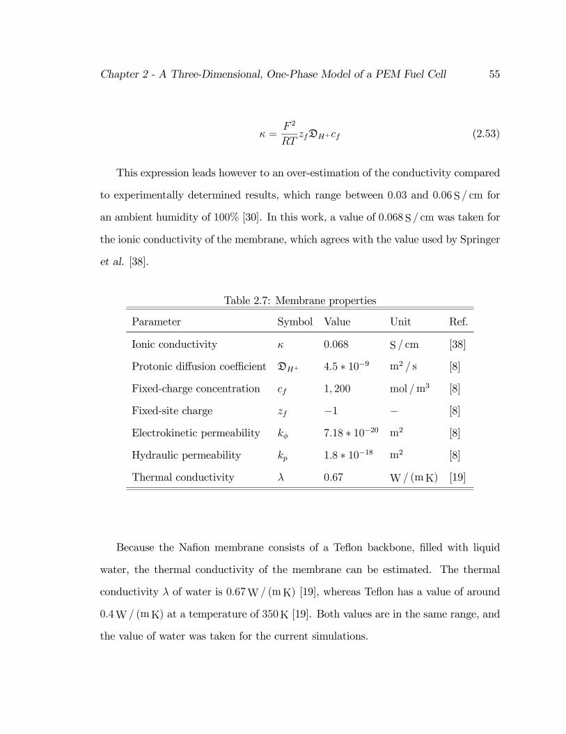
Chapter 2 - A Three-Dimensional, One-Phase Model of a PEM Fuel Cell 55
· =F 2
RTzfDH+cf (2.53)
This expression leads however to an over-estimation of the conductivity compared
to experimentally determined results, which range between 0:03 and 0:06 S = cm for
an ambient humidity of 100% [30]. In this work, a value of 0:068 S = cm was taken for
the ionic conductivity of the membrane, which agrees with the value used by Springer
et al. [38].
Table 2.7: Membrane properties
Parameter Symbol Value Unit Ref.
Ionic conductivity · 0:068 S = cm [38]
Protonic di¤usion coe¢cient DH+ 4:5 ¤ 10¡9 m2 = s [8]
Fixed-charge concentration cf 1; 200 mol =m3 [8]
Fixed-site charge zf ¡1 ¡ [8]
Electrokinetic permeability kÁ 7:18 ¤ 10¡20 m2 [8]
Hydraulic permeability kp 1:8 ¤ 10¡18 m2 [8]
Thermal conductivity ¸ 0:67 W = (mK) [19]
Because the Na…on membrane consists of a Te‡on backbone, …lled with liquid
water, the thermal conductivity of the membrane can be estimated. The thermal
conductivity ¸ of water is 0:67W = (mK) [19], whereas Te‡on has a value of around
0:4W = (mK) at a temperature of 350K [19]. Both values are in the same range, and
the value of water was taken for the current simulations.

Chapter 2 - A Three-Dimensional, One-Phase Model of a PEM Fuel Cell 56
2.8 Base Case Results
2.8.1 Validation Comparisons
In order to establish the accuracy of the numerical simulations, comparisons have to
be made with experimental results, where the …rst (and in many cases only) output is
the polarization curve. The results obtained in this model are being compared with
experimental results by Ticianelli et al. [42] and in a later chapter with data from
Kim et al. [20].
Ticianelli et al. [42] modelled their experimental results with an equation of the
form:
E = E0 ¡ b log (i) ¡ rii (2.54)
which models the obtained polarization curves and gives insight into the electrode
kinetic parameters for the oxygen reduction reaction and the ohmic losses. b in
this expression is the Tafel slope and ri is the internal resistance of the cell. The
assumptions made in this equation are that mass transport limitations and activation
overpotential at the hydrogen electrode are negligible.
Kim et al. [20] …tted their data to the following expression that also accounts for
the mass transport overpotential:
E = E0 ¡ b log (i) ¡ rii¡m exp(ni) (2.55)
where m and n were obtained through curve-…tting and are associated with mass
transport losses at high current densities.

Chapter 2 - A Three-Dimensional, One-Phase Model of a PEM Fuel Cell 57
E0 in the above equations is a constant and can be expressed by:
E0 = Er + b log (i0) (2.56)
where Er is the reversible cell potential for the cell and i0 is the exchange current den-
sity for the oxygen reduction reaction. Putting equations 2.54 and 2.56 together yields
the equation for the polarization curves neglecting mass transport overpotentials and
activation losses at the hydrogen electrode:
E = Er ¡ b logµii0
¶¡ rii (2.57)
where the logarithmic term can be recognized as corresponding to the Tafel equation.
Table 2.8 gives an example of the data presented by Ticianelli et al. [42]. Note that
the catalyst loading is 0:35mg Pt= cm2 for both PEM 21 and PEM 45.
Table 2.8: Experimental curve-…t data
Cell no. Cell type p [atm] T [±C] E0 [V] i0 [A = cm2] b [V =dec] ri
PEM 21 H2/Air 3/5 50 0.933 110£10¡9 0.072 0.23
PEM 21 H2/Air 3/5 75 0.945 277£10¡9 0.070 0.25
PEM 45 H2/Air 3/5 50 0.928 20£10¡9 0.062 0.69
PEM 45 H2/Air 3/5 80 0.935 104£10¡9 0.065 0.39
Figure 2.4 compares the results of the model at base case conditions with the
experimental results obtained by Ticianelli et al. [42]. The agreement between the
modelling results and experiments is good, especially for the low and intermediate cur-
rent densities. The increasing discrepancies in the cell potential towards high current

Chapter 2 - A Three-Dimensional, One-Phase Model of a PEM Fuel Cell 58
densities can be explained by mass transport limitations, which are not considered
in the empirical curve described by equation 2.57, but which were included in the
modelling results. This means that a comparison can only be made in the low and in-
termediate current density regions (up to ¼ 1:0A = cm2). In addition, there is a small
deviation in the slope of the linear section in the polarization curves, which indicates
that the protonic conductivity of the electrolyte membrane is slightly under-estimated
in the model. Finally, it has to be stated that the exact conditions of the experiments,
e.g. the stoichiometric ‡ow ratios used, channel geometries and electrode thickness
were not given, which makes it impossible to make de…nite quantitative comparisons.
What is important to note is that the current three-dimensional model gives realistic
results without ad-hoc adjustment to any of the parameters.
Current Density [A/cm2]
Cel
lVol
tage
[V]
Cel
lPow
er[W
/cm
2]
0.00 0.30 0.60 0.90 1.20 1.500.0
0.2
0.4
0.6
0.8
1.0
1.2
0.0
0.1
0.2
0.3
0.4
0.5
0.6Polarization Curve Ticianelli et. al.
Polarization Curve 3D Model
Power Density Curve 3D Model
Figure 2.4: Comparison of polarization curves and power density curves between the
3D modelling results and experiments.

Chapter 2 - A Three-Dimensional, One-Phase Model of a PEM Fuel Cell 59
In general, it is possible to obtain good agreement between a model and experi-
mental polarization curves with most models. Even the earlier one-dimensional model
of the MEA developed by Bernardi and Verbrugge [8] resulted in excellent agreement
between model and experiment with the adjustment of a single parameter. In the
model presented here, all the parameters are within physical limits, which will allow
us to conduct a systematic study on the importance of a single parameter on the fuel
cell performance. Whenever possible, experimental results will be shown as compar-
ison, but it has to be borne in mind that for the experiments that are published the
exact conditions are not given. Furthermore, experiments are con…ned to polarization
data, and detailed in-situ measurements are virtually non-existent.
One of the advantages of a comprehensive fuel cell model is that it allows for the
assessment of the di¤erent loss mechanisms, which is shown in Figure 2.5.
Current Density [A/cm2]
Pot
entia
l[V
]
0.0 0.2 0.4 0.6 0.8 1.0 1.2 1.40.0
0.2
0.4
0.6
0.8
1.0
1.2
CathodeActivation Loss
Cell Potential
AnodeActivation Loss
AnodeConcentration Loss
CathodeConcentration Loss
Membrane Loss
Ohmic Loss
Figure 2.5: The break-up of di¤erent loss mechanisms at base case conditions.

Chapter 2 - A Three-Dimensional, One-Phase Model of a PEM Fuel Cell 60
Due to the transfer coe¢cient of ® = 0:5 for the anode side reaction, the an-
odic activation loss increases relatively fast once the cell current density exceeds the
exchange current density of the anodic reaction. However, it should be possible to
alleviate anodic activation losses with improved catalyst deposition.
The most important loss mechanism is the activation overpotential at the cathode
side, which also has to be addressed with improved catalyst deposition techniques.
At high current densities, the membrane loss becomes signi…cant. It can be seen that
due to its ohmic nature, it increases linearly with increasing current density.
The cathode concentration loss is quantitatively small, until the oxygen concentra-
tion approaches zero at the limiting current density. Because the numerical solution
procedure can result in unrealizable negative mass fractions, when performing simu-
lations in this region, the mass transport limitation regime can not be well resolved.
2.8.2 Reactant Gas and Temperature Distribution Inside the
Fuel Cell
Due to the relatively low di¤usivity of the oxygen compared to the hydrogen, the
cathode operating conditions usually determine the limiting current density when
the fuel cell is run on humidi…ed air. This is because an increase in current density
corresponds to an increase in oxygen consumption. The concentration of oxygen at
the catalyst layer is balanced by the oxygen that is being consumed and the amount of
oxygen that di¤uses towards the catalyst layer, driven by the concentration gradient.
Therefore, we will, for the most part, limit the presentation of results mainly to the
cathode side of the fuel cell.

Chapter 2 - A Three-Dimensional, One-Phase Model of a PEM Fuel Cell 61
Figure 2.6 shows the reactant gas distribution inside the gas channels and at-
tached porous gas-di¤usion electrodes at a low current density. The depletion of the
reactant gases from the inlet (front) towards the outlet as well as the distribution
of the reactant gases inside the porous electrodes (wider parts of the “T”) is clearly
illustrated.
This plot demonstrates the e¤ect of the land area between two parallel channels
on the gas distribution. Due to the higher di¤usivity of the hydrogen the decrease in
molar concentration under the land areas is smaller than for the oxygen; the lowest
ratio between the minimum hydrogen concentration at the catalyst layer and the bulk
hydrogen concentration being 0:44=58. According to
i0 =µcH2
c1H2
¶1=2
(2.58)
the local current density varies of the square root of the local concentration of hydro-
gen [17, 44]. The result is a fairly even distribution of the local current density on
the anode side.
This is di¤erent at the cathode side, where the lower di¤usivity of the oxygen
along with the low concentration of oxygen in ambient air results in a noticeable
oxygen depletion under the land areas. Since, in addition, the local current density of
the cathode side reaction depends directly on the oxygen concentration (° = 1) [31],
this means that the local current density distribution under the land areas is much
smaller than under the channel areas, especially near the outlet.
This is even more pronounced at higher current densities, as Figure 2.7 demon-
strates. The gradients of the reactant gas distribution are steeper inside the di¤usion

Chapter 2 - A Three-Dimensional, One-Phase Model of a PEM Fuel Cell 62
layers, and the oxygen concentration is less than 2% throughout the entire catalyst
interface. Under the land areas it is almost zero, indicating that the limiting current
density has almost been reached. From this plot it becomes clear that the di¤usion
of the oxygen towards the catalyst layer is the main impediment for reaching high
current densities.
The molar oxygen concentration at the catalyst layer is shown in Figure 2.8. It
is interesting to note that the formation of the shoulders under the land areas is
strongest in the medium current density region. At a low current density, the oxygen
consumption rate is low enough not to cause di¤usive limitations, whereas at a high
current density the concentration of oxygen under the land areas has already reached
near-zero values and can not further decrease.
The temperature distribution inside the fuel cell for these current densities is
shown in Figure 2.9. Naturally, the maximum temperature occurs, where the electro-
chemical activity is highest, which is near the cathode side inlet area. However, the
temperature increase for low current densities is small, only 1K. We will see below
that for low- and intermediate current densities the local current density distribution
is fairly even, which keeps the heat release small.
This is di¤erent for high current densities. A much larger fraction of the current
is being generated near the inlet of the cathode side under the channel, as will be
shown in Chapter 2.8.3, and this leads to a signi…cantly larger amount of heat being
generated here. The maximum temperature is more than 4K above the gas inlet
temperature and it occurs inside the membrane. The gases leave the computational
domain at slightly elevated temperatures, i.e. at around 353:6K at 0:4A = cm2 and

Chapter 2 - A Three-Dimensional, One-Phase Model of a PEM Fuel Cell 63
at 355K at 1:4A = cm2. However, it has to be borne in mind that this computational
domain presents only a small fraction of a complete cell, where serpentine channels
might be several orders of magnitude longer than the section investigated here, so
that in a real fuel cell the gases would heat up more signi…cantly.
Overall, the temperature rise inside a fuel cell might be quite signi…cant, and
can not be neglected. On the other hand, one of the most prominent e¤ects on the
temperature …eld, the heat of evaporation and condensation, was not accounted for
in these computations, since the amount of water undergoing phase-change was not
known. Phase change has a signi…cant impact on the temperature distribution inside
the fuel cell, and vice versa, as will be shown with the extended model in Chapter 4.

Chapter 2 - A Three-Dimensional, One-Phase Model of a PEM Fuel Cell 64
0.00
0.01
0.02
0.03
0.04
0.05
Channel Length [m]0.0005
0.0010
0.0015
0.0020
Channel Width [m]
0.0005
0.0010
0.0015
0.0020
Cha
nnel
Hei
gth
[m]
0.18
0.16
0.14 0.11
0.17
0.16
0.14
0.12 0.10
0.15
0.16
0.13 0.11 0.09
0.14
0.12 0.10
0.13
0.12 0.10
0.08
XO20.20
0.18
0.16
0.14
0.12
0.10
0.08
0.06
0.0020
0.0025
0.0030
0.0035
Cha
nnel
Hei
gth
[m]
0.57
0.55
0.55
0.53
0.53
0.51
0.51
0.50
0.49
0.48
0.47
0.46
XH20.58
0.56
0.54
0.52
0.50
0.48
0.46
0.44
Figure 2.6: Reactant gas distribution in the anode channel and GDL (upper) and
cathode channel and GDL (lower) at a nominal current density of 0:4A = cm2 at base
case conditions.

Chapter 2 - A Three-Dimensional, One-Phase Model of a PEM Fuel Cell 65
0.00
0.01
0.02
0.03
0.04
0.05
Channel Length [m]0.0005
0.0010
0.0015
0.0020
Channel Width [m]
0.0005
0.0010
0.0015
0.0020
Cha
nnel
Hei
ght[
m]
0.16
0.10
0.04
0.18
0.16
0.12
0.06
0.16
0.12
0.06 0.14
0.10
0.04
0.14
0.12
0.08
0.02
0.02
0.02
0.02
0.02
XO20.20
0.16
0.12
0.08
0.04
0.00
0.0020
0.0025
0.0030
0.0035
Cha
nnel
Hei
ght[
m]
0.56
0.54
0.50
0.48
0.54
0.52
0.48
0.46
0.52
0.50
0.48
0.44
0.50
0.48
0.46
0.42
0.48
0.46
0.44
0.40
XH20.58
0.54
0.50
0.46
0.42
0.38
Figure 2.7: Reactant gas distribution in the anode channel and GDL (upper) and
cathode channel and GDL (lower) at a nominal current density of 1:4A = cm2 at base
case conditions.

Chapter 2 - A Three-Dimensional, One-Phase Model of a PEM Fuel Cell 66
0.00
0.01
0.02
0.03
0.04
0.05
Channel Length
0.0005
0.0010
0.0015
0.0020Channel W
idth
0.00
0.04
0.08
0.12
0.16
0.20
XO
2
0.00
0.01
0.02
0.03
0.04
0.05
Channel Length
0.0005
0.0010
0.0015
0.0020Channel W
idth
0.00
0.04
0.08
0.12
0.16
0.20
XO
2
0.00
0.01
0.02
0.03
0.04
0.05
Channel Length
0.0005
0.0010
0.0015
0.0020Channel W
idth
0.00
0.04
0.08
0.12
0.16
0.20
XO
2
0.00
0.01
0.02
0.03
0.04
0.05
Channel Length
0.0005
0.0010
0.0015
0.0020Channel W
idth
0.00
0.04
0.08
0.12
0.16
0.20
XO
2
0.00
0.01
0.02
0.03
0.04
0.05
Channel Length
0.0005
0.0010
0.0015
0.0020Channel W
idth
0.00
0.04
0.08
0.12
0.16
0.20
XO
2
0.00
0.01
0.02
0.03
0.04
0.05
Channel Length
0.0005
0.0010
0.0015
0.0020Channel W
idth
0.00
0.04
0.08
0.12
0.16
0.20
XO
2
Figure 2.8: Molar oxygen concentration at the catalyst layer for six di¤erent current
densities: 0:2A = cm2 (upper left), 0:4A = cm2 (upper right), 0:6A = cm2 (centre left),
0:8A = cm2 (centre right), 1:0A = cm2 (lower left) and 1:2A = cm2 (lower right).

Chapter 2 - A Three-Dimensional, One-Phase Model of a PEM Fuel Cell 67
0.00
0.01
0.02
0.03
0.04
0.05
Channel Length [m]0.0005
0.0010
0.0015
0.0020
Channel Width [m]
0.0005
0.0010
0.0015
0.0020
0.0025
0.0030
Cha
nnel
Hei
gth
[m]
353.50
353.70
354.00
353.60
353.40 353.90
353.50
353.80
353.70
353.30
353.70
353.60
353.60
353.20
353.40
T354.20
354.00
353.80
353.60
353.40
353.20
353.00
0.00
0.01
0.02
0.03
0.04
0.05
Channel Length [m]0.0005
0.0010
0.0015
0.0020
Channel Width [m]
0.0005
0.0010
0.0015
0.0020
0.0025
0.0030
Cha
nnel
Hei
gth
[m]
353.80
354.20
356.20
357.00
355.00
355.80
356.20
355.80
354.60
355.80
354.20
355.40
355.40354.60
355.00
355.00
T357.00
356.20
355.40
354.60
353.80
353.00
Figure 2.9: Temperature distribution inside the fuel cell at base case conditions for
two di¤erent nominal current densities: 0:4A = cm2 (upper) and 1:4A = cm2 (lower).

Chapter 2 - A Three-Dimensional, One-Phase Model of a PEM Fuel Cell 68
2.8.3 Current Density Distribution
It was noted before that one of the most critical variables for fuel cell modelling is
the local current density distribution. Once the detailed distribution of the reactant
gas at the catalyst is obtained with the model, it is possible to determine the local
current density distribution, assuming an even catalyst loading throughout the cell
and a constant activation overpotential.
Figure 2.10 shows the local current density distribution at the cathode side cat-
alyst layer for three di¤erent nominal current densities: 0:2A = cm2, 0:8A = cm2 and
1:4A = cm2. For the sake of comparison, the local current density has been nominal-
ized by divided through the average current density. It can be seen that for a low
nominal current density the local current is evenly distributed, the maximum being
just about 20% higher and the minimum 20% lower than the average (nominal) cur-
rent density. The result is an evenly distributed heat generation, as we have seen
before.
An increase in the nominal current density to 0:8A = cm2 leads to a more pro-
nounced distribution of the local current, and the maximum can exceed the average
current density by more than 70% at the cathode side inlet, the minimum being 50%
below the average. Further increase in the current leads to a more extreme current
distribution inside the cell.
For an average current density of 1:2A = cm2, a high fraction of the current is
generated at the catalyst layer that lies beneath the channels, leading to an under-
utilization of the catalyst under the land areas.

Chapter 2 - A Three-Dimensional, One-Phase Model of a PEM Fuel Cell 69
2.00
1.80
1.60
1.40
1.20
1.20
1.00 0.80 0.600.40
0.20
1.00 0.80 0.600.40
0.20
1.90
1.70
1.50
1.30
1.30
2.10
Channel Length [m]
Cel
lWid
th[m
]
0.00 0.01 0.02 0.03 0.04 0.050.0000
0.0005
0.0010
0.0015
0.0020
Land
Are
aC
hann
elA
rea
Land
Are
a
1.60
1.50
1.40
1.30
1.20
1.10
1.10
1.00
1.00
1.10 1.00 0.90 0.80 0.70 0.600.50
1.10 1.00 0.90 0.80 0.700.60
0.50
1.70
Channel Length [m]
Cel
lWid
th[m
]
0.00 0.01 0.02 0.03 0.04 0.050.0000
0.0005
0.0010
0.0015
0.0020
Land
Are
aC
hann
elA
rea
Land
Are
a
1.20
1.10
1.00
0.90
0.80
0.80
Channel Length [m]
Cel
lWid
th[m
]
0.00 0.01 0.02 0.03 0.04 0.050.0000
0.0005
0.0010
0.0015
0.0020
Land
Are
aC
hann
elA
rea
Land
Are
a
Figure 2.10: Dimensionless current density distribution i=iave at the cathode side cata-
lyst layer for three di¤erent nominal current densities: 0:2A = cm2 (upper), 0:8A = cm2
(middle) and 1:4A = cm2 (lower).

Chapter 2 - A Three-Dimensional, One-Phase Model of a PEM Fuel Cell 70
The resulting ratio of the overall current that is being generated under the channel
area is shown in Figure 2.11. At a low current density, around 50% of the total
current is generated under the channel area. This, however, increases rapidly in an
almost linear manner as the current density increases, and the maximum reaches
nearly 80% at the limiting current density. Overall, the simulations suggest a more
e¤ective catalyst utilization can be achieved with a non-uniform catalyst distribution,
by depositing a larger fraction of the catalyst under the land area and towards the
outlet of the fuel cell.
Current Density [A/cm2]
Cur
rent
Fra
ctio
n[%
]
0.0 0.5 1.0 1.550.0
60.0
70.0
80.0
Figure 2.11: Fraction of the total current generated under the channel area as opposed
to the land area.

Chapter 2 - A Three-Dimensional, One-Phase Model of a PEM Fuel Cell 71
2.8.4 Liquid Water Flux and Potential Distribution in the
Membrane
The current model assumes a fully humidi…ed membrane. In reality, the membrane
is prone to partly dehumidify at the anode side [38], which leads to a non-isotropic
electrical conductivity of the membrane. Nevertheless, the results for the water ‡ux
and the electrical potential distribution in the membrane shall be brie‡y discussed
here.
Figure 2.12 shows the ‡ow vectors of the liquid water through the membrane
and the electrical potential distribution in the membrane for three di¤erent current
densities. The liquid water ‡ux is governed by two e¤ects: the convection due to
the pressure di¤erential across the membrane and the electro-osmotic drag associated
with the transport of hydrogen protons from the anode to the cathode side. As the
electro-osmotic drag follows the direction of the electric current in the membrane and
the current is perpendicular to the iso-lines of the electrical potential, the drag is also
in the direction perpendicular to the electrical potential isolines.
At a low current density of 0:1A = cm2, the pressure gradient outweighs the ef-
fect of the electro-osmotic drag, and so the net water ‡ux is directed towards the
anode almost throughout the entire domain. Since the current is fairly uniformly dis-
tributed at the cathode side at low current densities, the electrical potential gradient
is relatively constant in the z-direction.
When the current density is increased to 0:2A = cm2, the e¤ect of the electro-
osmotic drag in the membrane starts to outweigh the e¤ect of the pressure gradient,

Chapter 2 - A Three-Dimensional, One-Phase Model of a PEM Fuel Cell 72
0.00
0.01
0.02
0.03
0.04
0.05
Cell Length [m]
0.0000
0.0005
0.0010
0.0015
0.0020
Cell Width [m]
0.04
0.03
0.02
0.01
0.010.020.030.04
0.010.02
0.03
0.010.02
0.03
0.010.02
0.03
0.00
0.01
0.02
0.03
0.04
0.05
Cell Length [m]
0.0000
0.0005
0.0010
0.0015
0.0020
Cell Width [m]
0.020.040.06
0.020.04
0.06
0.020.04
0.06
0.020.040.06
0.020.04
0.06
0.00
0.01
0.02
0.03
0.04
0.05
Cell Length [m]
0.0000
0.0005
0.0010
0.0015
0.0020
Cell Width [m]
0.1000.200
0.3000.4000.500
0.1000.200
0.3000.400
0.500
0.1000.2000.300
0.400
0.1000.2000.3000.400
0.1000.2000.3000.400
Figure 2.12: Liquid water velocity …eld (vectors) and potential distribution (contours)
inside the membrane at base case conditions for three di¤erent current densities:
0:1A = cm2 (upper), 0:2A = cm2 (middle) and 1:2A = cm2 (lower). The vector scale is
200 cm = (m = s), 20 cm = (m = s), and 2 cm = (m = s), respectively.

Chapter 2 - A Three-Dimensional, One-Phase Model of a PEM Fuel Cell 73
and the liquid water ‡ux is directed from the anode side to the cathode side through-
out the entire domain. The iso-potential lines are more and more curved around
the area between the fuel cell channels, as can be seen for the current density of
1:2A = cm2. This is due to the high local current densities in these areas.
It is important to note that the current density, at which the electro-osmotic drag
starts outweighing the pressure gradient, depends entirely on the modelling param-
eters used in the Schlögl equation, i.e. the electrokinetic permeability k© and the
hydraulic permeability kp of the membrane, both of which are di¢cult to determine.
The values used in the current calculations stem from [8], where k© = 7:18£10¡20m2
and kp = 1:8 £ 10¡18m2. Gurau et al. [17] used an electrokinetic permeability of
k© = 11:3 £ 10¡20m2 and a hydraulic permeability of kp = 1:58 £ 10¡18m2 in their
two-dimensional model, and their results predict that for otherwise similar conditions
the direction of the liquid water ‡ux changes between 0:8A = cm2 and 0:9A = cm2. In
both cases we note that the region, where the net water ‡ux inside the membrane
changes direction, is con…ned to a small current density range.
Another comparison can be made with the modelling results by Nguyen et al. [28],
[52]. This group described the water ‡ux inside the membrane by (i) electro-osmotic
drag, (ii) back-di¤usion by the concentration gradient of water created by the electro-
osmotic ‡ow from the anode side to the cathode side and the cathode side reaction
and (iii) convection by the pressure gradient between the anode side and the cathode
side of the channels:
~Nw;mem = nd~iF
¡ Dwrcw ¡ cwkp¹w
rp (2.59)
where nd is the electro-osmotic drag coe¢cient, i.e. the number of water molecules

Chapter 2 - A Three-Dimensional, One-Phase Model of a PEM Fuel Cell 74
dragged by each hydrogen proton that migrates through the membrane and Dw is the
di¤usion coe¢cient of water in the membrane. Note the similarity of this equation
with the well-established Nernst-Planck equation [4]:
~Ni = ¡ziFRT
Dicir© ¡ Dirci + ci~v (2.60)
Appendix B shows, how these expressions compare to the Schlögl equation. In
order to compare the results presented here with the model presented by Nguyen et
al., the electrokinetic permeability of the membrane in this model has to be adjusted
to k© = 2:0 £ 10¡20m2.
Figure 2.13 compares the modelling results for the net drag coe¢cient ® for both
values of the electrokinetic permeability k©. ® is de…ned as the net number of water
molecules that crosses the membrane per hydrogen proton. Reducing the electroki-
netic permeability leads to a decrease of ® from values around 3:0 ¡ 4:6 to values
below 1:0. The current density, where the water ‡ux changes direction has increased
from around 0:1A = cm2 to 0:4A = cm2.
For comparison, the ®-values obtained by Yi and Nguyen [52] are in the order of
0:6 ¡ 0:8 at a current density of 1:1A = cm2, and a pressure gradient of 1 atm and a
value between 0:8 and 1:0 in the absence of a pressure gradient. By adjusting the
electrokinetic permeability we have obtained ®-values that are of the same order of
magnitude.
Experimental values for the net drag coe¢cient ® have been obtained by Choi et
al. [12], who found that for current densities of 0:2A = cm2 and higher, the value is
constant at around 0:3. At lower current densities, however, the net drag coe¢cient

Chapter 2 - A Three-Dimensional, One-Phase Model of a PEM Fuel Cell 75
increases up to 0:55 at 0:06A = cm2, which must be attributed to the back-di¤usion.
The experiments were conducted without a pressure gradient using humidi…ed H2
and O2 as reactant gases.
Current Density [A/cm2]
#Wat
erM
olec
ules
/Pro
ton
0.0 0.5 1.0 1.55.0
4.0
3.0
2.0
1.0
0.0
1.0
2.0
3.0
4.0
5.0
k =2.00e20 m2φ
k =7.17e20 m2φ
Figure 2.13: Comparison of values for the net drag coe¢cient ® for two di¤erent
values of the electrokinetic permeability of the membrane.
Overall, the Schlögl equation does not appear to be su¢cient to describe the
‡ux of liquid water through the membrane. The parameters used in the equations
proved to be critical, yet di¢cult to determine. This will have to be addressed in
future extensions of this model. For the overall model evaluation, however, the water
management is not critical, because most of the experiments that we compare our
result with have been conducted under controlled conditions with humidi…ed inlet
gases so that the membrane was indeed fully humidi…ed.

Chapter 2 - A Three-Dimensional, One-Phase Model of a PEM Fuel Cell 76
2.8.5 Grid Re…nement Study
Because the conservation equations listed above in Chapter 2.4 are solved in their
…nite-di¤erence form, the discretization of the di¤erential equations on the grid should
become exact as the grid spacing tends to zero. The di¤erence between the discretized
equation and the exact one is called the truncation error. It is usually estimated
by replacing all the nodal values in the discrete approximation by a Taylor series
expansion about a single point. As a result one recovers the original di¤erential
equation plus a reminder, which represents the truncation error. For a method to be
consistent, the truncation error must become zero when the mesh spacing ¢xi ! 0
[15]. Truncation error is usually proportional to a power of the grid spacing ¢x
[15]. Consistency of the numerical method alone is not su¢cient in order to obtain
a converged solution. In addition, the method has to be stable, which means that
the method used does not magnify the errors that appear in the course of numerical
solution process. For an iterative method as it is used here, a stable method is one
that does not diverge [15].
A numerical method is said to be convergent if the solution of the discretized
equations tends to the exact solution of the di¤erential equation as the grid spacing
tends to zero. In order to check the convergence of a non-linear problem like the one
we are dealing with, convergence can only be investigated by numerical experiments,
i.e. repeating the calculation on a series of successively re…ned grids. If the method
is stable and all approximations used in the discretization process are consistent, we
will …nd that the computation does converge to a grid-independent solution.
In order to investigate this, the grid that has been shown in Figure 2.3 has been
re…ned twice by adding 20% of the cells and 40% of the cells in every direction,

Chapter 2 - A Three-Dimensional, One-Phase Model of a PEM Fuel Cell 77
respectively, leading to a 73% and a 174% …ner grid overall. The computations at
base case conditions were repeated on these re…ned grids, and the solutions compared.
The polarization curves obtained with the re…ned grids are shown in Figure 2.14,
left. It is almost impossible to distinguish the three di¤erent lines, which is also true
for the average molar oxygen fraction at the catalyst layer, shown on the right hand
side of Figure 2.14. This indicates that in terms of the fuel cell performance the base
case grid provides adequate resolution.
x
x
x
x
x
x
xx
x
Current Density [A/cm2]
Mol
arO
xyge
nF
ract
ion
[]
0.00 0.50 1.00 1.50 2.000.00
0.05
0.10
0.15
0.20
Base Case Grid
Refined by 20 %
Refined by 40 %x
x
x
x
x
x
x
xx
x
Current Density [A/cm2]
Cel
lPot
entia
l[V
]
0.00 0.50 1.00 1.50 2.000.00
0.20
0.40
0.60
0.80
1.00
Base Case Grid
Refined by 20 %
Refined by 40 %x
Figure 2.14: Polarization curves (left) and molar oxygen fraction at the catalyst layer
as a function of the current density (right) for three di¤erent grid sizes.
The local current density distribution at the cathodic catalyst layer for the three
di¤erent numerical grids is shown in Figure 2.15. Also shown is the grid used in every
case (white lines). Note that the y-axes are scaled by a factor of 10 compared to the
x-axes. The di¤erences in the current density distribution are very small. A the inlet
area at mid-channel the local current density is slightly higher for the coarse grid.
Apart from that, no di¤erences can be observed.

Chapter 2 - A Three-Dimensional, One-Phase Model of a PEM Fuel Cell 78
1.80 1.7
01.6
01.5
01.4
01.3
0
1.20
1.20
0.400.500.600.700.800.901.001.10
1.10
0.400.500.600.700.800.901.00
Channel Length [m]
Cel
lWid
th[m
]
0.00 0.01 0.02 0.03 0.04 0.050.0000
0.0005
0.0010
0.0015
0.0020
Land
Are
aC
hann
elA
rea
Land
Are
a
1.80
1.70 1.6
01.5
01.4
01.3
0
1.20
1.20
1.10
1.10
0.40
0.40
0.500.600.700.800.901.00
0.500.600.700.800.901.00
Channel Length [m]
Cel
lWid
th[m
]
0.00 0.01 0.02 0.03 0.04 0.050.0000
0.0005
0.0010
0.0015
0.0020
Land
Are
aC
hann
elA
rea
Land
Are
a
1.70
1.60
1.50
1.40
1.30
1.20
1.20
1.10
1.10
0.40
0.40
0.50
0.50
0.60
0.600.70
0.700.80
0.800.901.00
0.901.00
1.80
Channel Length [m]
Cel
lWid
th[m
]
0.00 0.01 0.02 0.03 0.04 0.050.0000
0.0005
0.0010
0.0015
0.0020
Land
Are
aC
hann
elA
rea
Land
Are
a
Figure 2.15: Local current distribution at the catalyst layer for three di¤erent grid
sizes: Base Case (upper), 120%£ Base Case (middle) and 140%£ Base Case (lower).
The nominal current density is 1:0A = cm2.
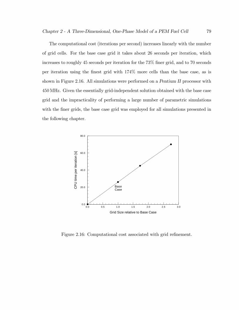
Chapter 2 - A Three-Dimensional, One-Phase Model of a PEM Fuel Cell 79
The computational cost (iterations per second) increases linearly with the number
of grid cells. For the base case grid it takes about 26 seconds per iteration, which
increases to roughly 45 seconds per iteration for the 73% …ner grid, and to 70 seconds
per iteration using the …nest grid with 174% more cells than the base case, as is
shown in Figure 2.16. All simulations were performed on a Pentium II processor with
450MHz. Given the essentially grid-independent solution obtained with the base case
grid and the impracticality of performing a large number of parametric simulations
with the …ner grids, the base case grid was employed for all simulations presented in
the following chapter.
Grid Size relative to Base Case
CP
Utim
epe
rite
ratio
n[s
]
0.0 0.5 1.0 1.5 2.0 2.5 3.00.0
20.0
40.0
60.0
80.0
BaseCase
Figure 2.16: Computational cost associated with grid re…nement.

Chapter 2 - A Three-Dimensional, One-Phase Model of a PEM Fuel Cell 80
2.8.6 Summary
A three-dimensional computational model of a PEM Fuel Cell has been presented
in this chapter. The complete set of equations was given, and the computational
procedure, based on the commercial software package CFX 4.3, was outlined. The
results of the base case show good agreement with experimentally obtained data, taken
from the literature. A detailed distribution of the reactants and the temperature …eld
inside the fuel cell for di¤erent current densities were presented. Water management
issues for the polymer membrane were addressed. A grid re…nement study revealed
that already for the coarsest grid that was used the solution proofed to be grid-
independent.
This model can be used to provide fundamental understanding of the transport
phenomena that occur in a fuel cell, and furthermore provide guidelines for fuel cell
design and prototyping. The following chapter will focus on a parametric study
employing the model presented here that was conducted in order to better understand
and ultimately predict the fuel cell performance under various operating conditions.
Operational, geometrical as well as material parameters were systematically varied in
order to assess their e¤ect on the fuel cell performance.

81
Chapter 3
A Parametric Study Using the
Single-Phase Model
3.1 Introduction
Next, a parametric study was conducted to (i) identify the critical parameters for fuel
cell performance, and (ii) determine the sensitivity of the model to various parameters
and hence identify which of these need to be speci…ed more accurately. In order to do
so, only one parameter was changed from the base case conditions at a time. Care had
to be taken on how other modelling parameters depend on the parameter that was
changed, i.e. the temperature in‡uences all other transport parameters inside the fuel
cell, ranging from the di¤usivities of the species to the speed of the electrochemical
reactions, and this had to be taken into account. Only three aspects of the results
will be emphasized during this chapter:
i. the limiting current density, which is reached when then oxygen consumption
at the catalyst layer can just be balanced by the supply of oxygen via di¤usion.

Chapter 3 - A Parametric Study Using the Single-Phase Model 82
In contrast to a two-dimensional model, the three-dimensional model presented
here is capable of making predictions about the limiting current density that
can be reached for the di¤erent geometries investigated. As will be seen in a
later chapter, the amount of spacing between the single fuel cell channels (land
area) has a strong impact on the onset of mass transport limitations, which can
not be captured by a two-dimensional model.
ii. the fuel cell performance in form of the polarization curves or power density
curves. Since the electrical power of the fuel cell is equal to the product of the
current density and the electrical potential, the polarization curve is equivalent
to the power density curve and vice versa. However, in some cases, the results
become clearer when considering the power density curve and in others the
polarization curves reveal more information.
iii. the local current density distribution at the catalyst layer. For an optimum fuel
cell performance and in order to avoid large temperature gradients inside the
fuel cell, it is desirable to achieve a uniform current density distribution inside
the cell.
The parameters investigated include the operating temperature and pressure, sto-
ichiometric ‡ow ratio, oxygen concentration of the incoming cathode stream, the
porosity and thickness of the GDL and the ratio between the channel width and the
land area.

Chapter 3 - A Parametric Study Using the Single-Phase Model 83
3.2 E¤ect of Temperature
The temperature basically a¤ects all the di¤erent transport phenomena inside the
fuel cell. Predominantly a¤ected are:
² the composition of the incoming gas streams. Assuming the inlet gases are fully
humidi…ed, the partial pressure of water vapour entering the cell depends on the
temperature only. Thus, the molar fraction of water vapour is a function of the
total inlet pressure and temperature, and so the molar fraction of the incoming
hydrogen and oxygen depend on the temperature and pressure as well.
² the exchange current density i0. The exchange current density of an electro-
chemical reaction depends strongly on the temperature. Parthasarathy et al.
[32] conducted experiments in order to determine a correlation between the cell
temperature and the exchange current density of the oxygen reduction reaction.
² the membrane conductivity ·. A higher temperature leads also to a higher
di¤usivity of the proton in the electrolyte membrane, thereby reducing the
membrane resistance.
² the reference potential E0. Although Equation 2.39 shows a decrease in the ref-
erence potential with an increasing temperature, experimental results indicate
an increase, which can be explained with a higher di¤usivity of the hydrogen
with increasing temperature [32].
² the gas-pair di¤usivities Dij in the Stefan-Maxwell equations. An increase in
temperature leads to an increase in the gas-pair di¤usivities.

Chapter 3 - A Parametric Study Using the Single-Phase Model 84
In order to determine the inlet gas composition as a function of temperature, the
following relation between the temperature and the saturation pressure of water has
been used [38]:
log10 psat = ¡2:1794 + 0:02953 £ #¡ 9:1837E ¡ 5 £ #2 + 1:4454E ¡ 7 £ #3 (3.1)
where # is the temperature in [±C]. The molar fraction of water vapour in the incoming
gas stream is simply the ratio of the saturation pressure and the total pressure:
xH2O;in =psatpin
(3.2)
Since the ratio of nitrogen and oxygen in dry air is known to be 79 : 21, the inlet
oxygen fraction can be found via:
xO2;in =1 ¡ xH2O;in
1 + 7921
(3.3)
and the molar nitrogen fraction can be determined out of:
xN2;in + xH2O;in + xO2;in = 1 (3.4)
The resulting inlet gas composition for di¤erent pressures is shown in Figure 3.1.
In order to …nd a correlation between the reference exchange current density i0
for the oxygen reduction reaction (ORR) at the cathode side and the temperature,
experimental results obtained by Parthasarathy et al. [32] were used. The following
relation has been obtained using a curve-…tting approach:
i0;'=5:2(T ) = 1:08 £ 10¡21 £ exp (0:086 ¤ T ) (3.5)

Chapter 3 - A Parametric Study Using the Single-Phase Model 85
Temperature [C]
Mol
arO
2F
ract
ion
[]
Mol
arH
2OF
ract
ion
[]
50 60 70 800.00
0.05
0.10
0.15
0.20
0.25
0.00
0.10
0.20
0.30
0.40
0.50
Water Vapour
5 atm
Oxygen
3 atm
1 atm
3 atm
1 atm
5 atm
Figure 3.1: Molar inlet fraction of oxygen and water vapour as a function of temper-
ature at three di¤erent pressures.
where T is the temperature in [K] and ' is the so-called roughness factor1. The
second column of Table 3.1 lists the exchange current densities obtained by applying
the above equation.
For the base case in our computational model we assume an exchange current
density of i0 = 4:4 ¤ 10¡7A = cm2 at a cell temperature of 353K [42]. Comparing this
with the value obtained by Parthasarathy et al., the roughness factor in our model
can be determined as:
1The roughness factor ' is de…ned as the ratio between the electrochemically active area and
the geometrical area of the cell, and it provides a measure the quality of the catalyst distribution.
The exchange current density of the oxygen reduction reaction is only of the order of 10¡9 ¡ 10¡10
A = cm2 [2]. In order to keep the activation losses within a reasonable range, however, the exchange
current density based on the geometrical area must be at least in the range of 10¡6 ¡ 10¡7 A = cm2.
This means that the electrochemically active area has to be at least two orders of magnitude higher
then the geometrical area of the fuel cell.

Chapter 3 - A Parametric Study Using the Single-Phase Model 86
'¤ = 5:2 £ 4:4 ¤ 10¡7
1:65 ¤ 10¡8= 138:4 (3.6)
Using this correction factor, all the exchange current densities that have been
found by Parthasarathy et al. were adjusted to the higher catalyst loading by linear
interpolation and thus the third column in Table 3.1 was obtained. It should be em-
phasized that for the current study it is important to obtain a qualitative estimation of
how the various parameters depend on the temperature. The experiments conducted
by Parthasarathy et al. and the experiments that we use for our base case taken
from Ticianelli et al. [42] were conducted under di¤erent (unknown) conditions. The
exchange current densities listed in the third column in Table 3.1 appear reasonable
and were therefore used for the current parametric study.
Table 3.1: Exchange current density of the ORR as a function of temperature
T i0;#=5:2(T ) i¤0;#=138:4(T )
353 1:65 £ 10¡8 4:4 £ 10¡7
343 6:99 £ 10¡9 1:86 £ 10¡7
333 2:96 £ 10¡9 7:86 £ 10¡8
323 1:25 £ 10¡9 3:33 £ 10¡8
Next, an expression had to be found for the protonic conductivity of the electrolyte
membrane as a function of temperature. A theoretical value was given by Bernardi
and Verbrugge [7] as:
· =F 2
RTzfDH+cf (3.7)

Chapter 3 - A Parametric Study Using the Single-Phase Model 87
where F is Faraday’s constant, R is the universal gas constant, zf and cf are the …xed
charge number and -concentration, respectively, T is the temperature in [K] and DH+
is the di¤usivity if the hydrogen proton inside the membrane,which depends strongly
on the temperature. The di¤usivity of the hydrogen proton was measured to be [7]
DH+ = 4:5 ¤ 10¡5 cm2 = s at 80 ±C and DH+ = 5:6 ¤ 10¡5 cm2 = s at 95 ±C. The second
column in Table 3.2 lists the values for the di¤usivity obtained by linear extrapolation
from these values, and the third column shows the theoretical membrane conductivi-
ties assuming a linear dependence of the protonic di¤usivity on the temperature.
These values, however, show a large deviation from experimentally measured pro-
tonic conductivities in an operating fuel cell. For example, Springer et al. [38]
obtained a value of · = 0:068 S = cm. Coincidentally, this value was also used by
Bernardi and Verbrugge [8] to match their modelling data with experimental results
from Ticianelli et al. [42]. Thus, this value was taken for our base case, and linearly
scaled as a function of temperature, based on the theoretical value from the third
column. The last column in Table 3.2 lists the adjusted values that were taken for
the membrane conductivity at di¤erent temperatures.
Table 3.2: Proton di¤usivity and membrane conductivity as function of temperature.
T [K] DH+ [cm2 = s] ·theo [S = cm] · [S = cm]
353 4:5 £ 10¡5 0:17 0:068
343 3:8 £ 10¡5 0:13 0:052
333 3:0 £ 10¡5 0:11 0:044
323 2:3 £ 10¡5 0:095 0:038

Chapter 3 - A Parametric Study Using the Single-Phase Model 88
As before, the adjustment of the reference exchange potential E0 with the cell
temperature is described by the Nernst equation:
E0 = 1:23 ¡ 0:9 £ 10¡3 (T ¡ 298) + 2:3RT4F
log¡p2H2pO2
¢(3.8)
Using these adjustments, the polarization curves obtained for various cell tem-
peratures are shown in Figure 3.2. The change in the initial drop due to the lower
exchange current density is relatively small compared to the drop-o¤ in the linear
region, caused by the ohmic losses. The maximum achievable current density in-
creases slightly with increasing operating temperature due to the overall enhanced
mass transport, i.e. by di¤usion of the reactants. For the power density curves it
has to be noted that the maximum power density is shifted towards a higher current
density with an increase in temperature, which is caused by the reduction in ohmic
losses.
Current Density [A/cm2]
Pow
erD
ensi
ty[W
/cm
2]
0.00 0.50 1.00 1.500.00
0.10
0.20
0.30
0.40
0.50
80 C
70 C
60 C
50 C
Current Density [A/cm2]
Cel
lPot
entia
l[V
]
0.00 0.50 1.00 1.500.00
0.20
0.40
0.60
0.80
1.00
80 C
70 C
60 C
50 C
Figure 3.2: Polarization Curves (left) and power density curves (right) at various
temperatures obtained with the model. All other conditions are at base case.

Chapter 3 - A Parametric Study Using the Single-Phase Model 89
For comparison, experimental results reproduced from Ticianelli et al. [42] are
shown in Figure 3.3. The polarization curves shown have been reproduced by using
the electrokinetic data given in Table 2.8 on page 57. Qualitatively, the e¤ect of the
operating temperature on the performance of both cells agrees well with the modelling
results presented above. Note that the di¤erence in performance between these two
cells is caused solely by the amount of Na…on impregnation at the catalyst layer.
PEM 45 used 4% instead of 3:3%, which lead to a ”starvation” of reactants at the
cathode side.
Current Density [A/cm2]
Cel
lPot
entia
l[V
]
0.00 0.30 0.60 0.90 1.200.00
0.20
0.40
0.60
0.80
1.00PEM21 75 C
PEM21 50 CPEM45 80 C
PEM45 50 C
Figure 3.3: Experimentally obtained polarization curves for di¤erent operating tem-
peratures.
Overall the modelling results exhibit good qualitative agreement with experimen-
tal data. However, in order to obtain this agreement, it is essential to understand the
impact that the temperature has on the various parameters of the model, which had
to be found experimentally.

Chapter 3 - A Parametric Study Using the Single-Phase Model 90
3.3 E¤ect of Pressure
Similar to the temperature, the operating pressure enhances numerous transport prop-
erties in a PEM Fuel Cell. The following adjustment have to be made to account for
a change in the operating pressure:
² the inlet gas compositions. A change in the operating pressure leads to a change
in the inlet gas compositions, assuming the inlet gases are fully humidi…ed.
² the exchange current density i0. The dependence of the cathodic exchange
current density on the oxygen pressure was investigated experimentally by
Parthasarathy et al. [31].
² the reference potential Eref . According to the Nernst equation, an increased
pressure leads to an increase in the equilibrium potential.
² the gas-pair di¤usivities Dij in the Stefan-Maxwell equations. It is well known
that the product of pressure and the binary di¤usivity is constant [13]. Hence,
a doubling of the pressure will cut the binary di¤usivity in half.
Since the saturation pressure for water is only a function of temperature, it remains
constant for a variation of the inlet pressure, and the molar fraction of water vapour
in the incoming cathode gas stream is given by equations 3.1 and 3.2. The molar
oxygen and nitrogen fractions result then out of equations 3.3 and 3.4. Figure 3.4
shows the resulting inlet gas composition at the cathode side as a function of the
pressure. It can be seen that the change in the inlet gas composition is particularly
strong in the range from 1 atm to 3 atm. Above 3 atm, the composition changes only
slightly with the pressure.

Chapter 3 - A Parametric Study Using the Single-Phase Model 91
Pressure [atm]
Mol
arH
2OF
ract
ions
[]
Mol
arO
2F
ract
ion
[]
1 2 3 4 50.00
0.10
0.20
0.30
0.40
0.50
0.00
0.05
0.10
0.15
0.20
0.25
Water Vapour
60 C
Oxygen
80 C
60 C60 C
70 C
70 C 80 C
Figure 3.4: Molar oxygen and water vapour fraction of the incoming air as a function
of pressure for three di¤erent temperatures.
log [PO2/atm]
i0[A
/cm
2]
0.5 0.0 0.5 1.0109
108
107
106
Experiments with air
Experiments with oxygen
Curve Fit: y=1.27E8*exp{2.06*x}
Figure 3.5: The dependence of the exchange current density of the oxygen reduction
reaction on the oxygen pressure.

Chapter 3 - A Parametric Study Using the Single-Phase Model 92
The exchange current density was scaled to qualitatively match experimental re-
sults obtained by Parthasarathy et al. [31], who determined the cathode side exchange
current density as a function of the partial oxygen pressure at a temperature of 50 ±C.
The results are summarized in Figure 3.5. A linear relationship was found between
the logarithm of the exchange current density i0 and the logarithm of the oxygen
partial pressure, according to:
i0 = 1:27 £ 10¡8 £ exp2:06¤PO2 (3.9)
This equation was applied to the partial oxygen pressure of the incoming air, as
listed in the second column of Table 3.3, to yield an approximation for the cathodic
exchange current at a temperature of 50 ±C, given in the third column of Table 3.3.
The last column was obtained by linearly interpolating the exchange current densities
in the third column so that the value for our base case, where the cathode side pressure
is 5 atm and the temperature is 80 ±C, is matched, according to:
i0 (80 ±C; ' = 138:4) = i0 (50 ±C) £ 4:4 £ 10¡7
9:27 £ 10¡8(3.10)
The values in the last column are the exchange current densities that were taken
to model the fuel cell under di¤erent pressures.
Again this method might appear somewhat arbitrary, but it has to be kept in
mind that for this part of the analysis it is important to understand the qualitative
impact that the operating pressure has on the di¤erent parameters and then …nd a
quantitative expression that represents this as closely as possible.

Chapter 3 - A Parametric Study Using the Single-Phase Model 93
Table 3.3: Exchange current density of the ORR as a function of pressure
pc[atm] pO2 [atm] i0 (pc; T = 50 ±C) i0 (pc; T = 80 ±C)
1:0 0:1251 1:64 £ 10¡8 0:78 £ 10¡7
1:5 0:1483 1:72 £ 10¡8 0:82 £ 10¡7
3:0 0:5451 3:90 £ 10¡8 1:85 £ 10¡7
5:0 0:9650 9:27 £ 10¡8 4:40 £ 10¡7
The adjustment of the reference potential E0 was done according to the corrected
Nernst equation (equation 2.39), and the di¤usion coe¢cients for the Stefan-Maxwell
equations were adjusted automatically in our model.
The result of the computations with varying operation pressure is shown in Figure
3.6. The higher oxygen fraction at the cathode side inlet leads eventually to a higher
maximum current density, as can be seen in the left part of Figure 3.6. This increase
is signi…cant when the pressure is increased from atmospheric pressure up to 3 atm,
which corresponds well with Figure 3.4. A further increase in the pressure from
3:0 atm to 5:0 atm does not lead to a signi…cant improvement in terms of the limiting
current density. It should be emphasized again that this is only valid as long as the
incoming gases are fully humidi…ed. The reason why even at extremely low current
densities the average molar oxygen fraction at the catalyst layer di¤ers from the value
of the incoming air is discussed in Chapter 3.4.
The polarization curves on the right hand side of Figure 3.6 reveal a signi…cant
change in the initial drop-o¤, when the pressure is changed. This can be attributed
to the change in the equilibrium potential that goes along with a decrease in the
reactant pressure (Nernst equation). To a much lesser extend, the decrease in the

Chapter 3 - A Parametric Study Using the Single-Phase Model 94
exchange current density with decreasing pressure also contributes to this e¤ect.
Current Density [A/cm2]
Mol
arO
xyge
nF
ract
ion
[]
0.00 0.50 1.00 1.500.00
0.05
0.10
0.15
0.20
p 5.0 atm
p 3.0 atm
p 1.5 atm
p 1.0 atm
Current Density [A/cm2]
Cel
lPot
entia
l[V
]
0.00 0.50 1.00 1.500.00
0.20
0.40
0.60
0.80
1.00
p 5.0 atm
p 3.0 atm
p 1.5 atm
p 1.0 atm
Figure 3.6: The molar oxygen fraction at the catalyst layer vs. current density (left)
and the polarization curves (right) for a fuel cell operating at di¤erent cathode side
pressures. All other conditions are at base case.
Again, a detailed comparison with experimental results from the literature can
only be made on a qualitative basis, since the exact conditions of the various exper-
iments are not reported. In Figure 3.7, experimentally obtained polarization curves
by Kim et al. [20] are reproduced. The experiments were conducted with pure hy-
drogen at the anode side and air at the cathode side. Although the exact details of
the experiments, such as the stoichiometric ‡ow ratio and the cell geometry, are not
known, the two main e¤ects that the cathode side pressure has on the fuel cell per-
formance can be observed for both temperatures: the increase of the limiting current
density with an increase in pressure and an overall better cell performance, which
can be attributed to an increase in the equilibrium potential. It is interesting to note
that at 50 ±C the limiting current densities for 3:0 atm and 5:0 atm almost coincide,

Chapter 3 - A Parametric Study Using the Single-Phase Model 95
which agrees well with the modelling results shown above. On the other hand, the
polarization curves for 3:0 atm and 5:0 atm at the elevated temperature were very
close, which is also in good agreement with the modelling results at a temperature of
80 ±C.
Current Density [A/cm2]
Cel
lPot
entia
l[V
]
0.00 0.20 0.40 0.60 0.80 1.00 1.20 1.400.00
0.20
0.40
0.60
0.80
1.00
p 5.0 atm
p 3.0 atm
p 1.0 atm
Current Density [A/cm2]
Cel
lPot
entia
l[V
]
0.00 0.20 0.40 0.60 0.80 1.00 1.20 1.400.00
0.20
0.40
0.60
0.80
1.00
p 5.0 atm
p 3.0 atm
p 1.0 atm
Figure 3.7: Experimentally obtained polarization curves at two di¤ferent tempera-
tures (left: 50 ±C; right: 70 ±C) for various cathode side pressures.
In general, it is di¢cult to compare the results obtained with the current model
with experimental results taken from the literature, since various parameters that are
not given in the literature in‡uence the fuel cell performance. Qualitative agreement,
however, is very good and the principal physical bene…ts of operating a fuel cell at
an elevated pressure have been con…rmed.

Chapter 3 - A Parametric Study Using the Single-Phase Model 96
3.4 E¤ect of Stoichiometric Flow Ratio
According to equation 2.42, an increase in the stoichiometric ‡ow ratio means simply
that the velocity of the incoming gas has to be increased with all remaining parameters
remaining constant. The result is an increase in the molar oxygen fraction at the
catalyst layer, as can be observed in Figure 3.8. Note that even at a current density
of almost zero, the molar oxygen fraction does not reach its inlet value of around
19%. The reason for this is the constant stoichiometric ‡ow ratio even at low current
densities, which means that the air leaving the cell will always be depleted of oxygen
by a signi…cant amount, and the plot in Figure 3.8 shows the average molar oxygen
fraction from the inlet to the outlet and under the land area.
Current Density [A/cm2]
Pow
erD
ensi
ty[W
/cm
2]
0.00 0.40 0.80 1.20 1.600.00
0.10
0.20
0.30
0.40
0.50
Stoich 4.0
Stoich 3.0
Stoich 2.0
Stoich 1.5
Current Density [A/cm2]
Mol
arO
xyge
nC
once
ntra
tion
[]
0.00 0.40 0.80 1.20 1.600.00
0.05
0.10
0.15
0.20
Stoich 4.0
Stoich 3.0
Stoich 2.0
Stoich 1.5
Figure 3.8: Molar oxygen fraction at the catalyst layer as a function of current density
(left) and power density curves (right) for di¤erent stoichiometric ‡ow ratios.
The increments of the gain in the limiting current density become smaller as the
stoichiometric ‡ow ratio increases, i.e. the gain in the maximum cell current when

Chapter 3 - A Parametric Study Using the Single-Phase Model 97
the stoichiometric ‡ow ratio is increased from ³ = 1:5 to ³ = 2:0 is about as large as
the gain for an increase from ³ = 2:0 to ³ = 3:0. The bene…ts for a further increase
to ³ = 4:0 is considerably smaller.
Since there is a price to pay for an increase in the stoichiometric ‡ow ratio, there
must be an optimum, where the gain in the cell performance just balances the ad-
ditional costs of a more powerful blower. This will have to be carefully considered,
when designing the fuel cell system.
The right hand side of Figure 3.8 shows that the potential gain in power density
is relatively small. This, however, is only valid as long as the cell is not ”starved” of
oxygen at a current density that is below the point that corresponds to the maximum
power density, which in turn depends on the exact cell geometry and the properties
of the materials that are used.
The e¤ect of the stoichiometric ‡ow ratio on the local current distribution is shown
in Figure 3.9. An increase in the stoichiometric ‡ow ratio from 2:0 to 4:0 leads to
a decrease in the maximum local current density from above 2:2A = cm2 to below
1:9A = cm2 at the inlet area. This is further reduced to below 1:8 A = cm2, if the
stoichiometric ‡ow ratio is increased to ³ = 4:0. Overall, a stoichiometric ‡ow ratio
of ³ = 3:0 appears to be optimum in terms of cell performance.
It is important to realize that the e¤ect of the stoichiometric ‡ow ratio on the water
management can not be assessed with the current model. The amount of incoming
air determines, how much water vapour can be carried out of the cell. This question
can only be addressed with a two-phase model.

Chapter 3 - A Parametric Study Using the Single-Phase Model 98
2.1
2.0
1.9
1.8 1.
71.6
1.5 1.
41.3
1.2
1.1
1.0
1.0
0.30.40.50.60.70.80.91.01.1
0.30.40.50.60.70.80.91.01.1
Channel Length [m]
Cel
lWid
th[m
]
0.00 0.01 0.02 0.03 0.04 0.050.0000
0.0005
0.0010
0.0015
0.0020
Land
Are
aC
hann
elA
rea
Land
Are
a
1.8 1.7 1.6 1.5 1.4 1.3
1.2
1.2
0.40.50.60.70.80.91.01.1
1.1
0.40.50.60.70.80.91.0
Channel Length [m]
Cel
lWid
th[m
]
0.00 0.01 0.02 0.03 0.04 0.050.0000
0.0005
0.0010
0.0015
0.0020
Land
Are
aC
hann
elA
rea
Land
Are
a
1.7 1.6 1.5 1.4 1.3
1.2
1.2
1.1
1.1
0.40.50.60.70.80.91.0
0.40.50.60.70.80.91.0
Channel Length [m]
Cel
lWid
th[m
]
0.00 0.01 0.02 0.03 0.04 0.050.0000
0.0005
0.0010
0.0015
0.0020
Land
Are
aC
hann
elA
rea
Land
Are
a
Figure 3.9: Local current density distribution for three di¤erent stoichiometric ‡ow
ratios: ³ = 2:0 (top), ³ = 3:0 (middle) and ³ = 4:0 (bottom). The average current
density is 1:0A = cm2.

Chapter 3 - A Parametric Study Using the Single-Phase Model 99
3.5 E¤ect of Oxygen Enrichment
In order to alleviate mass transport losses at the cathode side, the incoming air
stream is sometimes enriched with oxygen. The e¤ect of using pure oxygen instead
of air has been experimentally determined by Kim et al. [20]. Figure 3.10 shows the
polarization curves of a fuel cell operating at two di¤erent pressures at a temperature
of 50 ±C for both air and pure oxygen. The obtainable current densities are more
than 80% higher for all di¤erent cathode side pressures. The di¤erences in the initial
drop-o¤ at low current densities are now understood in light of the dependence of the
equilibrium potential on the oxygen pressure.
Current Density [A/cm2]
Cel
lPot
entia
l[V
]
0.00 0.30 0.60 0.90 1.20 1.500.00
0.20
0.40
0.60
0.80
1.00
Air 1 atm
Air 3 atmO2 1 atm
O2 3 atm
Figure 3.10: Experimentally measured fuel cell performance at 50 ±C for air and pure
oxygen as the cathode gas.
Using our three-dimensional model we compared the performance of the base case
with oxygen enriched air, where the molar oxygen fraction of the incoming cathode
gas stream has been increased to 25% and 30%, respectively. The resulting cell
performance is shown in Figure 3.11. The left hand side shows again the molar

Chapter 3 - A Parametric Study Using the Single-Phase Model 100
oxygen concentration at the cathodic catalyst layer as a function of the nominal
current density. The higher inlet fraction of oxygen is carried over to the catalyst
layer, i.e. the lines remain equidistant to one another. This ultimately leads to a
tremendous increase in the limiting current density. It will be shown later that the
slope of the molar oxygen fraction vs. current density lines depends on the geometry
of the fuel cell, i.e. the thickness and porosity of the carbon …ber paper and the ratio
of the channel width to the land area.
The right-hand side in Figure 3.11 shows the polarization curves for the three
di¤erent cases. All curves are quite similar until the mass transport limitations start
a¤ecting the performance. For the case with an oxygen inlet fraction of 30%, no mass
transport losses occur and the polarization curve follows a straight line. In this case
the ohmic losses, which occur predominantly in the membrane become the limiting
factor for achieving even higher current densities.
Current Density [A/cm2]
Mol
arO
xyge
nC
once
ntra
tion
[]
0.00 0.40 0.80 1.20 1.60 2.00 2.40 2.800.00
0.05
0.10
0.15
0.20
0.25
0.30
XO2in 0.30
XO2in 0.25
XO2in 0.19
Current Density [A/cm2]
Cel
lPot
entia
l[V
]
0.00 0.40 0.80 1.20 1.60 2.00 2.40 2.800.00
0.20
0.40
0.60
0.80
1.00
XO2in 0.30
XO2in 0.25
XO2in 0.19
Figure 3.11: Molar oxygen fraction at the catalyst layer as a function of current
density (left) and polarization curves (right) for di¤erent oxygen inlet concentrations.

Chapter 3 - A Parametric Study Using the Single-Phase Model 101
3.6 E¤ect of GDL Porosity
The porosity of the gas-di¤usion layer a¤ects the performance of the fuel cell in two
aspects: a higher void fraction provides less resistance for the reactant gases to reach
the catalyst layer on one hand, but in turn it leads to a higher contact resistance, as
will be described below.
An increase in the porosity " enhances the di¤usion of the species towards the
catalyst layer, as can be seen from the Bruggemann correction [33]:
Deffij = Dij"1:5 (3.11)
In addition, the gas-phase permeability is a¤ected in a way described in Appendix
C. However, the convection described by Darcy’s law plays only a minor role for the
‡ux of the species towards the catalyst layer; the main contribution was found to be
di¤usion, particularly at the low hydraulic permeability chosen for the base case.
Figure 3.12 shows the molar oxygen fraction at the catalyst layer for di¤erent
values of the porosity. Here we observe that the gradient of the oxygen concentration
versus the current density changes with the porosity of the GDL. Starting from ap-
proximately the same value at a very low current density (0:01A = cm2), the oxygen
concentration decreases rapidly with increasing current density at low values for the
porosity, resulting in a limiting current density of only 0:75A = cm2. On the other
hand, when the porosity is increased from " = 0:4 to " = 0:5, the limiting current
density increases from around 1:4A = cm2 to around 2:4A = cm2, which constitutes an
increase of around 70%.

Chapter 3 - A Parametric Study Using the Single-Phase Model 102
Current Density [A/cm2]
Pow
erD
ensi
ty[W
/cm
2]
0.00 0.40 0.80 1.20 1.60 2.00 2.400.00
0.10
0.20
0.30
0.40
0.50
0.60
Eps 0.4
Eps 0.3
Eps 0.5
Current Density [A/cm2]
Mol
arO
xyge
nF
ract
ion
[]
0.00 0.40 0.80 1.20 1.60 2.00 2.400.00
0.05
0.10
0.15
0.20
Eps 0.3
Eps 0.4
Eps 0.5
Figure 3.12: Average molar oxygen concentration at the catalyst layer (left) and
power density curves (right) for three di¤erent GDL porosities.
The right hand side of Figure 3.12, however, shows that the power density de-
creases rapidly after the maximum power has been reached. All three power density
curves are very close, because the negative impact of an increased porosity on the
ohmic loss is small and is partly o¤set by the bene…cial e¤ect that results out of a
reduction in the mass transport loss. At a porosity of 0:3, however, the cathode side
is starved of oxygen before the maximum power density has been reached. Hence, it is
important to keep the porosity at a maximum level in order to avoid starvation. This
demonstrates the importance of avoiding the accumulation of liquid water inside the
GDL, since this will reduce the pore-size available for the gas-phase and thus enhance
mass transport losses.
As mentioned above, another loss mechanism that is important when considering
di¤erent GDL porosities is the contact resistance. Contact resistances occur at all
interfaces of di¤erent materials and components, and in many cases their contribution

Chapter 3 - A Parametric Study Using the Single-Phase Model 103
to the fuel cell performance is small. The most important contact resistance occurs at
the interface of the bipolar plates and the outer surfaces of the membrane-electrode
assembly, the carbon …ber paper. The magnitude of this resistance depends on various
parameters, including the material used, the surface preparation and the mechanical
pressure imposed on the stack.
In the base case, a contact resistance of 0:006 cm2 was assumed. However, this
value depends on so many parameters that it is worthwhile exploring, how the fuel
cell performance is a¤ected by a change in the contact resistance, i.e. by a change in
the stack pressure. Since it can be assumed that the contact resistance varies linearly
with the area of the surfaces that are in contact, the contact resistance is a linear
function of the porosity ".
Figure 3.13 shows the power density curves for a contact resistance of 0:03 cm2
and 0:06 cm2, respectively. Already for a value of 0:03 cm2 the maximum power
density for a porosity of " = 0:4 is higher than for " = 0:5. This e¤ect is even
stronger, when a contact resistance of 0:06 cm2 is assumed. Note also the decrease
in the maximum current density at a porosity of " = 0:5 due to the increase in ohmic
losses, which means that in this case the limiting current density is determined by
the membrane loss instead of the onset of mass transport limitations.

Chapter 3 - A Parametric Study Using the Single-Phase Model 104
Current Density [A/cm2]
Cel
lPow
erD
ensi
ty[W
/cm
2 ]
0.00 0.50 1.00 1.50 2.000.00
0.10
0.20
0.30
0.40
0.50
0.60
Eps 0.3
Eps 0.4
Eps 0.5
Current Density [A/cm2]
Cel
lPow
erD
ensi
ty[W
/cm
2 ]
0.00 0.50 1.00 1.50 2.000.00
0.10
0.20
0.30
0.40
0.50
0.60
Eps 0.3
Eps 0.4
Eps 0.5
Figure 3.13: Power density curves for three di¤erent GDL porosities at two values for
the contact resistance: Rc = 0:03 cm2 (left) and Rc = 0:06 cm2 (right).
Another the bene…cial e¤ect of a high GDL porosity is to even out the local current
densities, as can be seen in Figure 3.14. Whereas the maximum local current density
exceeds 1:8A = cm2 near the inlet area for a porosity of " = 0:4, this value is reduced
to about 1:5A = cm2 for a porosity of " = 0:5 and 1:4A = cm2 for " = 0:6; the local
current density becomes much more evenly distributed with an increase in porosity.
Overall, the porosity of the GDL has been found to be a very sensitive parameter
for the fuel cell performance, as it has a large in‡uence on the limiting current density,
and, since the contact losses depend on it in a linear manner, it also a¤ects the fuel
cell performance in form of the maximum power density.

Chapter 3 - A Parametric Study Using the Single-Phase Model 105
1.80 1.7
01.6
01.5
01.4
01.3
0
1.20
1.20
0.400.500.600.700.800.901.001.10
1.10
0.400.500.600.700.800.901.00
Channel Length [m]
Cel
lWid
th[m
]
0.00 0.01 0.02 0.03 0.04 0.050.0000
0.0005
0.0010
0.0015
0.0020
Land
Are
aC
hann
elA
rea
Land
Are
a
1.50
1.40
1.30
1.20
1.10
1.00
1.00
0.600.700.800.901.001.10
0.600.700.800.901.001.10
Channel Length [m]
Cel
lWid
th[m
]
0.00 0.01 0.02 0.03 0.04 0.050.0000
0.0005
0.0010
0.0015
0.0020
Land
Are
aC
hann
elA
rea
Land
Are
a
1.40
1.30 1.
201.10
1.00
0.90
0.90
0.700.800.901.00
0.700.800.901.001.10
1.10
Channel Length [m]
Cel
lWid
th[m
]
0.00 0.01 0.02 0.03 0.04 0.050.0000
0.0005
0.0010
0.0015
0.0020
Land
Are
aC
hann
elA
rea
Land
Are
a
Figure 3.14: Local current densities for three di¤erent GDL porosities: " = 0:4 (top),
" = 0:5 (middle) and " = 0:6 (bottom). The average current density is 1:0A = cm2
for all cases.

Chapter 3 - A Parametric Study Using the Single-Phase Model 106
3.7 E¤ect of GDL Thickness
Next, the e¤ect of the GDL thickness shall be investigated. In theory, a thinner GDL
reduces the mass transport resistance as well as ohmic losses, which are relatively
small because of the high conductivity of the carbon …ber paper.
Figure 3.15 shows the average molar oxygen fraction at the catalyst layer as a
function of the current density. For current densities below 0:3A = cm2 the molar
oxygen fraction decreases with an decreasing GDL thickness. We will see below that
the reason for this behaviour is that a thinner GDL prevents the oxygen from di¤using
in the z-direction from the channel area towards the land area. At a high current
density the reduced resistance to the oxygen di¤usion by the thinner layer becomes
important, and the molar fraction at the catalyst layer increases with a decreasing
GDL thickness, thus increasing the limiting current density.
Current Density [A/cm2]
Pow
erD
ensi
ty[W
/cm
2]
0.00 0.40 0.80 1.20 1.60 2.00 2.400.00
0.10
0.20
0.30
0.40
0.50
0.60
t = 0.140 mm
t = 0.200 mm
t = 0.260 mm
Current Density [A/cm2]
Mol
arO
xyge
nC
once
ntra
tion
[]
0.00 0.40 0.80 1.20 1.60 2.00 2.400.00
0.05
0.10
0.15
0.20
t = 0.140 mm
t = 0.200 mm
t = 0.260 mm
Figure 3.15: Molar oxygen concentration at the catalyst layer as a function of the
current density and the power density curves for three di¤erent GDL thicknesses.

Chapter 3 - A Parametric Study Using the Single-Phase Model 107
The e¤ect of the GDL thickness on the polarization curve and the power density
curve is small, because the only parameters a¤ected are the mass transport losses –
which is quantitatively a weak e¤ect – and the ohmic losses inside the GDL, which
are almost negligible. Therefore, the power density curves show di¤erences only
at high current densities. Overall, the predominant e¤ect of the GDL thickness is
on the limiting current density. There also might be issues concerning the water
management, but as before, these can not be addressed with the current version of
this model.
The fact that at low current densities the oxygen concentration is lower at the
catalyst layer for a thinner GDL than for the thicker GDL is an interesting aspect
of this di¤usion problem and shall be brie‡y discussed here. Figures 3.16 and 3.17
show in detail the molar oxygen concentration at the catalyst layer for the three
di¤erent GDL at a low and a high current density, respectively. At a current density
of 0:2A = cm2 the oxygen consumption is low. For the thicker GDL, the “space” for
the oxygen to di¤use in the lateral (z-) direction is larger than for a thinner GDL. As
a result, the oxygen concentration under the land area is higher for the thicker GDL.
And although the concentration under the channel areas is higher for the thinner
GDL, the average concentration remains lower for this case.
At a current density of 1:2A = cm2 the di¤usion in the y-direction is clearly the
limiting factor and constitutes the limitation that eventually determines the maximum
current density of the fuel cell. For the thicker GDL, the average molar oxygen fraction
is around 2:1%, which has already been observed in Figure 3.15, whereas the thinner
GDL allows for a higher oxygen fraction and ultimately a higher limiting current
density.

Chapter 3 - A Parametric Study Using the Single-Phase Model 108
0.17
0.16
0.15
0.14
0.13
0.12
0.090.100.110.120.13
0.14
0.090.100.110.120.130.14
Cell Length [m]
Cel
lWid
th[m
]
0.00 0.01 0.02 0.03 0.04 0.050.0000
0.0005
0.0010
0.0015
0.0020
Land
Are
aC
hann
elA
rea
Land
Are
a
0.17
0.16
0.15
0.14
0.13
0.12
0.100.110.120.130.14
0.100.110.120.130.14
Cell Length [m]
Cel
lWid
th[m
]
0.00 0.01 0.02 0.03 0.04 0.050.0000
0.0005
0.0010
0.0015
0.0020
Land
Are
aC
hann
elA
rea
Land
Are
a
0.16
0.15
0.14
0.13
0.12
0.110.120.130.140.15
0.110.120.130.140.15
0.17
Cell Length [m]
Cel
lWid
th[m
]
0.00 0.01 0.02 0.03 0.04 0.050.0000
0.0005
0.0010
0.0015
0.0020
LC
hann
elA
rea
Land
Are
aLa
ndA
rea
Figure 3.16: Molar oxygen concentration at the catalyst layer for three di¤erent GDL
thicknesses: 140¹m (upper), 200¹m (middle) and 260¹m (lower). The nominal
current density is 0:2A = cm2.

Chapter 3 - A Parametric Study Using the Single-Phase Model 109
0.10
0.09
0.08
0.07
0.06
0.06
0.010.02
0.030.040.05
0.010.02
0.030.040.05
Cell Length [m]
Cel
lWid
th[m
]
0.00 0.01 0.02 0.03 0.04 0.050.0000
0.0005
0.0010
0.0015
0.0020
Land
Are
aC
hann
elA
rea
Land
Are
a
0.07
0.06
0.05
0.010.02
0.03
0.04
0.04
0.010.02
0.03
Cell Length [m]
Cel
lWid
th[m
]
0.00 0.01 0.02 0.03 0.04 0.050.0000
0.0005
0.0010
0.0015
0.0020
Land
Are
aC
hann
elA
rea
Land
Are
a
0.04 0.03
0.02
0.01
0.02
0.01
Cell Length [m]
Cel
lWid
th[m
]
0.00 0.01 0.02 0.03 0.04 0.050.0000
0.0005
0.0010
0.0015
0.0020
Cha
nnel
Are
aLa
ndA
rea
Land
Are
a
Figure 3.17: Molar oxygen concentration at the catalyst layer for three di¤erent GDL
thicknesses: 140¹m (upper), 200¹m (middle) and 260¹m (lower). The nominal
current density is 1:2A = cm2.

Chapter 3 - A Parametric Study Using the Single-Phase Model 110
3.8 E¤ect of Channel-Width-to-Land-Area Ratio
Two di¤erent e¤ects determine the ideal ratio between the width of the gas ‡ow
channel and the land area between the channels. A reduction in the land area width
enhances the mass transport of the reactants to the catalyst layer that lies under the
land area. It is expected that this will a¤ect mainly the limiting current density and
to a lesser degree the voltage drop due to mass transport limitations. On the other
hand, a reduced width of the land area increases the contact resistance between the
bipolar plates and the membrane-electrode assembly. Since this is an ohmic loss, it
is expected to be directly correlated to the land area width.
Again, the molar oxygen fraction and the power density curves for three di¤erent
ratios between the land area and the channel width is shown in Figure 3.18.
Current Density [A/cm2]
Mol
arO
xyge
nC
once
ntra
tion
[]
0.00 0.50 1.00 1.50 2.000.00
0.05
0.10
0.15
0.20
Ch/L: 0.8mm/1.2mm
Ch/L: 1.0mm/1.0mm
Ch/L: 1.2mm/0.8mm
Current Density [A/cm2]
Pow
erD
ensi
ty[W
/cm
2]
0.00 0.50 1.00 1.50 2.000.00
0.10
0.20
0.30
0.40
0.50
Ch/L: 0.8mm/1.2mm
Ch/L: 1.0mm/1.0mm
Ch/L: 1.2mm/0.8mm
Figure 3.18: Average molar oxygen fraction at the catalyst layer as a function of
current density (left) and power density curves (right) for three di¤erent channel and
land area widths.

Chapter 3 - A Parametric Study Using the Single-Phase Model 111
Similar to other parameters, the width of the gas ‡ow channel mainly a¤ects
the limiting current density; a reduction in the channel width to 0:8mm results in
a decrease in the limiting current density from 1:42A = cm2 to 1:2A = cm2 (15:5%),
whereas an increase in the channel width from 1:0mm to 1:2mm along with a decrease
in the land area results in a limiting current density of 1:65A = cm2 (16:1%), i.e. equal
steps for an increase in the channel width result in equal increases in the limiting
current density.
The power density is weakly a¤ected, as can be seen on the left-hand side of Figure
3.18. For the case of the narrow channel, mass transport limitations start to become
noticeable at 1:0A = cm2, and the maximum of the power density occurs at this current
density. For an increased channel width from 1:0mm to 1:2mm, the maximum in
the powered density stays roughly the same at around 1:1A = cm2, because the mass
transport limitations only occur at higher current densities.
Figure 3.19 depicts the local current distribution for the three cases investigated.
As with previously investigated parameters, the channel width has a large impact
on the local current density distribution. For the narrow channel the local current
density can exceed 2:2A = cm2, and a large fraction of the overall current is being
generated under the channel area. This maximum value is reduced to a value between
1:5A = cm2 and 1:6A = cm2 for a wider channel of 1:2mm.
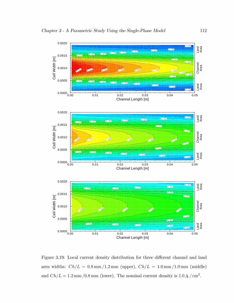
Chapter 3 - A Parametric Study Using the Single-Phase Model 112
2.20 2.10 2.00 1.90 1.80 1.70 1.60
1.50
1.40
1.40
1.30
1.30
0.200.300.400.500.600.700.800.901.10
0.200.300.400.500.600.700.800.901.00
Channel Length [m]
Cel
lWid
th[m
]
0.00 0.01 0.02 0.03 0.04 0.050.0000
0.0005
0.0010
0.0015
0.0020
Land
Are
aC
hann
elA
rea
Land
Are
a
1.80 1.7
01.6
01.5
01.4
01.3
0
1.20
1.20
0.400.500.600.700.800.901.001.10
1.10
0.400.500.600.700.800.901.00
Channel Length [m]
Cel
lWid
th[m
]
0.00 0.01 0.02 0.03 0.04 0.050.0000
0.0005
0.0010
0.0015
0.0020
Land
Are
aC
hann
elA
rea
Land
Are
a
0.500.600.700.800.90
1.50 1.
401.30
1.20
1.10
1.00
1.00
0.90
0.90
0.500.600.700.800.90
Channel Length [m]
Cel
lWid
th[m
]
0.00 0.01 0.02 0.03 0.04 0.050.0000
0.0005
0.0010
0.0015
0.0020
Land
Are
aC
hann
elA
rea
Land
Are
a
Figure 3.19: Local current density distribution for three di¤erent channel and land
area widths: Ch=L = 0:8mm =1:2mm (upper), Ch=L = 1:0mm =1:0mm (middle)
and Ch=L = 1:2mm =0:8mm (lower). The nominal current density is 1:0A = cm2.

Chapter 3 - A Parametric Study Using the Single-Phase Model 113
Finally, as mentioned before, the contact resistance between the graphite plates
and the carbon …ber paper plays an important role, when judging the advantages of a
wider channel. Again, a contact resistance of 0:03 cm2 and 0:06 cm2 was assumed,
respectively. At an assumed contact resistance of 0:03 cm2 all three di¤erent cases
perform equally well in terms of the maximum power density. With a further increase,
the case with the highest contact area starts to outperform the other two cases. Again,
it has to be stretched that the values for the contact resistance are pure assumptions;
it is not clear, how high the resistance can be under realistic operating conditions.
Current Density [A/cm2]
Cel
lPow
erD
ensi
ty[W
/cm
2 ]
0.00 0.50 1.00 1.50 2.000.00
0.10
0.20
0.30
0.40
0.50Ch/L: 0.8mm/1.2mm
Ch/L: 1.0mm/1.0mm
Ch/L: 1.2mm/0.8mm
Current Density [A/cm2]
Cel
lPow
erD
ensi
ty[W
/cm
2 ]
0.00 0.50 1.00 1.50 2.000.00
0.10
0.20
0.30
0.40
0.50Ch/L: 0.8mm/1.2mm
Ch/L: 1.0mm/1.0mm
Ch/L: 1.2mm/0.8mm
Figure 3.20: Power density curves for di¤erent assumed contact resistances:
0:03 cm2 (left) and 0:06 cm2 (right).

Chapter 3 - A Parametric Study Using the Single-Phase Model 114
3.9 Summary
A detailed analysis of the fuel cell performance under various operating conditions
has been conducted and the e¤ects of temperature, pressure, stoichiometric ‡ow ratio,
oxygen content of the incoming air, as well as GDL thickness and porosity and chan-
nel width have been examined. In order to achieve good agreement with experimental
results, functional relationships had to be developed between operating parameters,
such as temperature and pressure, and input parameters for the computational model
such as the exchange current density of the oxygen reduction reaction. The analysis
helped identifying critical parameters and shed insight into the physical mechanisms
leading to a fuel cell performance under various operating conditions. Furthermore,
the study performed in this chapter helped to explain previously published experi-
mental results by di¤erent research groups without knowledge of the exact conditions.
One of the major simpli…cations of the current model is the assumption that the
volume of the liquid water inside the gas di¤usion layers is negligible. Moreover, the
gas and liquid phase are treated in separate computational domains, neglecting the
interaction between the liquid water and the gas phase. In order to eliminate this
shortcoming, a two-phase model has been developed, which will be presented in the
following chapter.

115
Chapter 4
A Three-Dimensional, Two-Phase
Model of a PEM Fuel Cell
4.1 Introduction
Using as a basis the one-phase model presented in Chapter 2, a two-phase model has
been developed that accounts for both the gas and liquid phase in the same compu-
tational domain and thus allows for the implementation of phase change inside the
gas di¤usion layers. In addition, the computational domain was extended to include
a cooling channel, which will allow to assess the impact of the coolant temperature
and ‡ow rate on the amount of liquid water inside the MEA under various operating
conditions.
The multi-phase model presented here is di¤erent from those in the literature in
that it is three-dimensional as opposed to two-dimensional (e.g. [18], [49]). Further-
more, it is non-isothermal and accounts for the physics of phase change in that the

Chapter 4 - A Three-Dimensional, Two-Phase Model of a PEM Fuel Cell 116
rate of evaporation is a function of the amount of liquid water present and the level
of undersaturation. The addition of a cooling channel is also a unique feature of the
present model and enhancing its physical realism. Finally, the model is not limited
to relatively low humidity reactants, as was the case in prior two-phase ‡ow studies,
and can be used to simulate conditions representative of actual fuel cell operation.
Similar to the models by Hen et al. [18] and Wang et al. [49], the current two
phase study focuses on the gas-di¤usion layer and the ‡ow channels, neglecting the
membrane. However, in contrast to these authors, the anode side is included in
the present model as well. Water transport inside the porous gas di¤usion layer is
described by two physical mechanisms: viscous drag and capillary pressure forces.
Liquid water, created by the electrochemical reaction and condensation, is dragged
along with the gas phase. It will be shown below that at the cathode side, the
humidity level of the incoming air determines whether this drag is directed into or
out of the gas di¤usion layer, whereas at the anode side this drag is always directed
into the GDL. The capillary pressure gradient drives the liquid water out of the gas
di¤usion layers into the ‡ow channels. This model is capable of identifying important
parameters for the wetting behaviour of the gas di¤usion layers and can be used
to identify conditions that might lead to the onset of pore plugging, which has a
detrimental e¤ect of the fuel cell performance.
The simulations performed with the model will also show that phase change of
water is controlled by three di¤erent, competing mechanisms: a rise in temperature
leads to a rise in the saturation pressure and hence causes evaporation; the depletion
of the reactants inside the gas-di¤usion layers causes an increase in the partial pressure
of the water vapour and can thus lead to condensation, whereas the pressure drop

Chapter 4 - A Three-Dimensional, Two-Phase Model of a PEM Fuel Cell 117
inside the gas di¤usion layers leads to a decrease in the pressure of the water vapour,
and hence can cause evaporation.
4.2 Modelling Domain and Geometry
The modelling domain for the two-phase case is shown in Figure 4.1. The cooling
water channel can be seen in the bottom of the domain. Because of the symmetry
conditions applied, only one quarter of the channel has to be included. Since the
liquid and the gas-phase are now accounted for in the same computational domain,
the Subdomain II from the single-phase model is not required. However, heat transfer
between the solid matrix and the gas-phase inside the gas-di¤usion layers is still
accounted for in the same fashion as in the single phase model (Subdomain I).
Figure 4.1: The modelling domain used for the two-phase computations.

Chapter 4 - A Three-Dimensional, Two-Phase Model of a PEM Fuel Cell 118
Subdomain III, which was used to calculate the electrical potential inside the
membrane, has been left out. The reason is that in the single phase model the
potential distribution inside the membrane was used to calculate the liquid water
‡ux, as described by the Schlögl equation. This, however, was found to be insu¢cient,
and more elaborate models of the electrolyte membrane are highly empirical, with an
unknown range of validity (e.g. Springer et al. [38]).
4.3 Assumptions
The assumptions made in the two-phase model are basically identical to the ones
stated in Chapter 2.3. In order to implement the phase change of water, the following
additional assumptions were made:
1. liquid water exists in the form of small droplets of speci…ed diameter only,
2. inside the channels the liquid phase and the gas phase share the same pressure
…eld,
3. equilibrium prevails at the interface of the water vapour and liquid water,
4. no other species exist in the liquid phase, i.e. it consists of liquid water only,
5. heat transfer between the gas-phase and the liquid water is idealized, i.e. both
phases share the same temperature …eld, and
6. phase change occurs only within the porous electrodes, i.e. phase change of
water inside the channels or at the channel/wall interfaces is not accounted for.

Chapter 4 - A Three-Dimensional, Two-Phase Model of a PEM Fuel Cell 119
The …rst assumption has been made in order to …nd an expression for the rate of
evaporation of water. However, it will be shown that the assumed size of the droplets
has no impact on the modelling results, indicating “fast” evaporation.
The remaining assumptions are standard for the treatment of a multi-phase prob-
lem. The last assumption leads to exceedingly high relative humidities inside the
‡ow channels, particularly when cooling is applied. However, for the current case we
are predominantly interested in the phase change that occurs inside the electrodes
in order to obtain the relative humidity at the electrode/membrane interface. The
problem of having strong condensation terms at the channel/wall interfaces and the
eventual appearance of rivulets is a complicated mathematical problem in itself and
beyond the scope of this thesis.
4.4 Modelling Equations
The approach taken for the current model is to subdivide every control volume into
volume fractions for the gas- and liquid phase. Hence, two sets of conservation equa-
tions for mass, momentum and energy are solved, which include the volume fraction
of every phase. Mathematically, this approach is similar to the one taken for the
‡ow through porous media, where the porosity was introduced in the Navier-Stokes
equations to account for the reduced space available for the gas phase. However, in
the multi-phase model, exchange terms exist between both phases, caused, for exam-
ple, by the phase change of water. Thus, the volume fractions become part of the
solution, and they result out of the mass conservation equations and the fact that the
sum over all the volume fractions has to be equal to unity.

Chapter 4 - A Three-Dimensional, Two-Phase Model of a PEM Fuel Cell 120
4.4.1 Main Computational Domain
Gas Flow Channels
The mass conservation equation for each phase yields the volume fraction r and
along with the momentum equations the pressure distribution inside the channels.
For the liquid phase the mass conservation equation has been adjusted to account for
a di¤usive term. This is coherent with the assumption that the liquid in the channel
consists of small droplets only. Mathematically, this is expressed via:
r ¢¡rg½gug
¢= 0 (4.1)
for the gas phase and
r ¢ (rl½lul) = r ¢ (½lDlrrl) (4.2)
for the liquid phase.
Two sets of momentum equations are solved in the channels, and it is assumed
that they share the same pressure …eld:
pg = p1 = p (4.3)
Under these conditions, it can be shown that the momentum equations reduce to [6]:
r ¢h³½gug ug ¡ ¹g
³rug+(rug)
T´´i
= ¡rgrp (4.4)
and
r ¢h³½lul ul ¡ ¹l
³rul+(rul)
T´´i
= ¡rlrp (4.5)

Chapter 4 - A Three-Dimensional, Two-Phase Model of a PEM Fuel Cell 121
Note that this form of the momentum equation assumes incompressible ‡ow, which
is the case for the liquid phase and a good approximation for the gas phase for a
Ma Á 0:3 [6].
Currently, no interaction between the phases in the form of a drag coe¢cient is
considered inside the ‡ow channels for the sake of simplicity.
The energy equation for each phase becomes:
r ¢£rg
¡½gugHg ¡ ¸grTg
¢¤= 0 (4.6)
and
r ¢ [rl (½lulHl ¡ ¸lrTl)] = 0 (4.7)
Multiple species are considered in the gas phase only, and the species conservation
equation in multi-component, multi-phase ‡ow becomes:
r ¢£rg
¡½gugygi ¡ ½gDgiirygi
¢¤= r ¢ rg½gDgijrygj (4.8)
where the term on the right-hand side arises because of the multi-component di¤usion,
as described in Appendix A. Note that in the two-phase case we are only dealing
with a binary mixture at the anode side, i.e. hydrogen and water vapour. In this
case, it can be shown that the source term on the right hand side becomes zero and
the di¤usivity Dgii reduces to the binary di¤usivity of the two components [39].
The constitutive equations are the same as in the single phase case, that is the
liquid phase is considered incompressible so that

Chapter 4 - A Three-Dimensional, Two-Phase Model of a PEM Fuel Cell 122
½l = ½w (4.9)
and the ideal gas assumption leads to:
½gi =pgMiRT; (4.10)
with the bulk density being:
1½g
=X ygi½gi
(4.11)
The sum of all mass fractions is equal to unity
Xygi = 1; (4.12)
and the molar fraction x is related to the mass fraction by:
xgi =ygiMiP ygiMi
: (4.13)
Overall, the ‡ow in the channel is described as a standard dispersed two-phase
‡ow, where the inter-phase drag is so strong that the velocity …eld is the same for
both phases. The gas phase is considered as an ideal gas, and the liquid phase is
incompressible. A change in the equations has been made in order to allow di¤usion
of the liquid droplets in the gas phase as a consequence of the small size of the droplets
assumed.

Chapter 4 - A Three-Dimensional, Two-Phase Model of a PEM Fuel Cell 123
Gas Di¤usion Layers
For the conservation of mass, mass transfer in the form of evaporation and conden-
sation is accounted for, so that the mass conservation equation results in:
r ¢¡(1 ¡ s) "½gug
¢= _mevap + _mcond (4.14)
and
r ¢ (s"½lul) = ¡ ( _mevap + _mcond) (4.15)
Note that the saturation s is the same as the liquid water volume fraction rl and
has been introduced in order to keep with common notation. Since the sum of all
volume fractions has to be equal to unity, the volume fraction of the gas phase rg
becomes (1 ¡ s). In every given control volume, either evaporation or condensation
can occur, depending on the relative humidity. The sign de…nition adopted here is
positive for evaporation and negative for condensation.
The momentum equation for the gas-phase is again reduced to Darcy’s law, which
is, however, based on the relative permeability for the gas phase kgp. The relative
permeability accounts for the reduction in pore volume available for one phase due
to the existence of the second phase [47]. Di¤erent approaches can be adapted to
mathematically describe of the relative permeability, the simplest of which has been
used in the current model [18]:
kgp = (1 ¡ s) ¢ k0p (4.16)
and
klp = s ¢ k0p (4.17)

Chapter 4 - A Three-Dimensional, Two-Phase Model of a PEM Fuel Cell 124
where k0p is the permeability of the dry electrode and s is again the saturation of
liquid water inside the GDL [18]. With this, the momentum equation for the gas
phase inside the gas di¤usion layer becomes:
ug = ¡kgp
¹grpg = ¡ (1 ¡ s) k
0p
¹grpg (4.18)
Transport of the liquid water is considered via two mechanisms: a shear term
drives the liquid phase along with the gas phase in the direction of the pressure
gradient, and capillary forces drive the liquid water from regions of high saturation
towards regions of low saturation [18]. Starting from Darcy’s law, we can write:
ul = ¡klp
¹lrpl (4.19)
where the liquid water pressure results out of the gas-phase pressure pg and the
capillary pressure pc according to [47]:
rpl = rpg ¡ rpc = rpg ¡ @pc@s
rs (4.20)
Introducing this expression into Equation 4.19 yields for the liquid water velocity
…eld:
ul = ¡klp
¹lrpg +
klp¹l
@pc@s
rs = ¡sk0p
¹lrpg ¡ D (s)rs (4.21)
where the di¤usivity D (s) is de…ned as [47]:
D (s) = ¡sk0p
¹l
@pc@s
(4.22)

Chapter 4 - A Three-Dimensional, Two-Phase Model of a PEM Fuel Cell 125
For the description of the capillary pressure as a function of the saturation pc (s),
Leverett [24] has shown that under idealized conditions the capillary pressure versus
saturation data can be cast in the following form:
pc = ¾µ"k0p
¶1=2
f (s) (4.23)
where ¾ is the interfacial liquid/gas tension, " is the porosity and the function f (s)
is determined using Udell’s expression [43]:
f (s) = 1:417 (1 ¡ s) ¡ 2:12 (1 ¡ s)2 + 1:263 (1 ¡ s)3 (4.24)
which has also been adopted by Wang et al. [49].
Di¤erent species are only considered in the gas phase, and the species conservation
equation is the same as in the one-phase computations, except for the consideration
of the volume fraction for each phase rg:
r ¢£rg
¡"g½gugygi ¡ "g½gDgiirygi
¢¤= "gr ¢
¡rg½gDgijrygj
¢(4.25)
This equation makes it obvious that the subdivision of a control volume into
volume fractions is analogous to considering a porous medium, where only part of the
control volume is accessible to the gas phase: rg and "g are inter-changeable, except
that rg is a variable that is solved for by the continuity equations. The term on the
right hand side is again due to the multi-species di¤usion, as described in Chapter
2.4. Equation 4.25 is valid for species that do not undergo phase change.
For the water vapour inside the gas phase, the equation reads as follows:

Chapter 4 - A Three-Dimensional, Two-Phase Model of a PEM Fuel Cell 126
r ¢£rg
¡"g½gugygw ¡ "g½gDgiirygw
¢¤= "g
£r ¢
¡rg½gDgijrygw
¢+ _mevap + _mcond
¤
(4.26)
where only one of the phase change terms can exist, evaporation or condensation.
Because of the sign convention adopted here the condensation term is negative (see
below).
The energy equation becomes:
r ¢£rg
¡"g½gughtot ¡ "g¸grTg
¢¤= ¯ (Ts ¡ Tg) ¡ "g ( _mevap + _mcond)¢hevap (4.27)
where ¢hevap denotes the heat of evaporation or condensation in [J = kg] at 80 ±C.
The gas phase and the liquid phase are assumed to be in thermodynamic equilibrium,
hence the temperature of the liquid water is the same as the gas phase temperature.
Implementation of Phase Change An important feature of this model is that
it accounts for the physics of phase change, which has so far been neglected in other
studies. The multi-phase model by Wang et al. [49] is based for instance on an isother-
mal assumption. In that work the relative humidity of water is calculated throughout
the domain, and if it exceeds 100%, it is concluded that condensation happens here,
whereas if it is less than 100% in the presence of liquid water, evaporation occurs.
The amount of water undergoing phase-change is calculated a posteriori, based on
consideration of the calculated concentration of water in any given control volume
versus the saturation concentration, based on the saturation pressure as a function
of temperature. This approach has one distinct weakness: the heat of evaporation

Chapter 4 - A Three-Dimensional, Two-Phase Model of a PEM Fuel Cell 127
and condensation for the amount of water undergoing phase change is not accounted
for. Consequently, the saturation pressure is always constant due to the isothermal
assumption.
The e¤ect of the temperature distribution on phase change is generally well un-
derstood and can be described as follows: when the (fully saturated) gas reaches the
vicinity of the catalyst layer of the fuel cell, it heats up due to the heat produced
by the electrochemical reaction. Consequently, the temperature increases. Since the
saturation pressure is a function of temperature only, it increases as well, and the
gas becomes undersaturated. This undersaturation creates a driving mechanism for
the evaporation of liquid water, which is formed during the electrochemical reaction.
Hence, phase change occurs already at the inlet area of the cathode gas. This evap-
oration induces cooling of the gas phase. This shows that there is a …ne balance for
evaporation/condensation, with the temperature being the determining factor. Ob-
viously, an isothermal model can not account for that, and has a limited physical
representation.
In order to account for the magnitude of phase change that occurs inside the GDL,
an expression had to be found that relates the level of over- and undersaturation as
well as the amount of liquid water to the rate of phase change.
Initially, the focus was directed on the expression for evaporation. This must be
related to (i) the level of undersaturation of the gas phase in each control volume
and (ii) the surface area of the liquid water in the control volume. The surface area
can be assumed proportional to the volume fraction of the liquid water in each cell.
An obvious choice for the shape of the liquid water is droplets, especially because the

Chapter 4 - A Three-Dimensional, Two-Phase Model of a PEM Fuel Cell 128
catalyst area is coated with Te‡on. In addition, the rate of evaporation of a single
droplet in a free stream is well understood.
The evaporation of a droplet in a convective stream has been described by Bird,
Steward and Lightfoot [10]. The ‡ux of water due to phase change is:
_Nw = kxm¼D2xw0 ¡ xw11 ¡ xw0
(4.28)
where D is the diameter of the droplet, xw0 is the molar concentration of water
at the interface, xw1 is the bulk concentration of water vapour (in this case the
molar concentration of water vapour in each control volume), kxm is the transfer
rate of water in [mol = (m2 s)] and _Nw is the ‡ux of water from the liquid phase
into the gas phase in [mol = s]. The bulk concentration xw1 is known by solving the
continuity equation of water. For the concentration of water vapour at the surface,
thermodynamic equilibrium between the liquid phase and the gas phase is assumed.
Under that condition, the surface concentration can be calculated out of the saturation
pressure at the temperature of the control volume.
The mass transfer coe¢cient kxm is analogous to a heat transfer coe¢cient, and
reliable correlations are available for the heat transfer coe¢cient for convection around
a sphere, so that the mass transfer coe¢cient kxm [10] can be obtained from:
kxm =cgDwgD
"2:0 + 0:60
µDv1½g¹g
¶1=2 µ¹g½gDwg
¶1=3#
(4.29)
where cg is the concentration of air in [mol =m3], Dwg is the di¤usion coe¢cient of
water-vapour in air in [m2 = s], v1 is the free-stream velocity in [m = s] and ½g is the

Chapter 4 - A Three-Dimensional, Two-Phase Model of a PEM Fuel Cell 129
air density in [kg =m3]. All these properties can be easily calculated to facilitate the
implementation of phase change.
It is assumed that all droplets have a speci…ed diameter D, and the number of
droplets in each control volume is found by dividing the total volume of the liquid
phase in each control volume by the volume of one droplet:
nD;CV =rlVCV16¼D
3(4.30)
The foregoing derivation is valid for a single drop in free convection. Because of
the uncertainty about the droplet size, along with the fact that inside the porous
medium we are not dealing with free convection, the overall expression is scaled by a
factor $:
_Nw = $nD;CV cgDwg
"2:0 + 0:60
µDv1½g¹g
¶1=2 µ¹g½gDwg
¶1=3#¼Dxw0 ¡ xw11 ¡ xw0
(4.31)
When the solution indicates that the relative humidity inside the porous medium
is close to 100% for several orders of magnitude of $ smaller than 1:0; the rate of
evaporation is indeed fast enough to justify the assumption made by other groups of
having a fully humidi…ed gas phase.
Finally, in order to obtain the mass ‡ux caused by evaporation, the above expres-
sion has to be multiplied with the molar mass of water, which results in the amount
of water undergoing evaporation in [kg = s] in each control volume:
_mevap =MH2O$nD;CV kxm¼Dxw0 ¡ xw11 ¡ xw0
(4.32)

Chapter 4 - A Three-Dimensional, Two-Phase Model of a PEM Fuel Cell 130
In case the relative humidity exceeds 100%, condensation occurs and the evapo-
ration term is switched o¤. The case of condensation is more complex, because it can
occur on every solid surface area, but the rate of condensation changes depending on
the surface conditions such as the water coverage [3]. In addition, the overall sur-
face area in each control volume available for condensation shrinks with an increasing
amount of liquid water present. It is currently assumed that the rate of condensation
depends only on the level of oversaturation of the gas phase multiplied by a constant.
For high levels of liquid saturation, this expression will have to be revised in the
future.
_mcond = $Cxw0 ¡ xw11 ¡ xw0
(4.33)
Note that because in this case the bulk concentration xw1 exceeds the surface
concentration resulting out of the temperature, xw0, the overall mass ‡ux through
condensation is negative, i.e. from the gas phase to the liquid phase.
Catalyst Layers
The sink and source terms applied at the catalyst layer are the same as those in
Chapter 2.4, except that the source term for liquid water at the cathode side is now
accounted for in the main computational domain:
SH2O(l) =MH2Oi2F
(4.34)
where the local current density i is again obtained using the Butler-Volmer equation
under the assumption of a constant activation overpotential.

Chapter 4 - A Three-Dimensional, Two-Phase Model of a PEM Fuel Cell 131
Bipolar Plates
As before, only conductive heat transfer is accounted for in the bipolar plates. The
equation solved is:
r ¢ (¸grrT ) = 0 (4.35)
where the subscript “gr” denotes graphite.
Water Cooling Channel
In the channels, the Navier-Stokes equations for laminar, incompressible ‡ow are
solved. These are the continuity equation:
r ¢ (½lul) = 0; (4.36)
the momentum equation:
r ¢ (½lul ul ¡ ¹lrul) = ¡rµpl +
23¹lr ¢ ul
¶+ r ¢
h¹l (rul)
Ti
(4.37)
and the energy equation:
r ¢ (½lulHl ¡ ¸lrTl) = 0: (4.38)
where the total enthalpy H is calculated out of the static (thermodynamic) enthalpy
h via:
Hl = hl +12u2l ; (4.39)
The ‡uid in the cooling channels is assumed to be liquid water only, hence, no
additional species equation need to be solved.

Chapter 4 - A Three-Dimensional, Two-Phase Model of a PEM Fuel Cell 132
4.4.2 Computational Subdomain I
The equations solved in this computational domain correspond exactly to the ones
given in Chapter 2.4.
4.5 Boundary Conditions
For the main computational domain, the same boundary conditions are applied as
in the one-phase model. Again, the inlet velocity is a function of the desired current
density and the stoichiometric ‡ow ratio. The gas streams entering the cell are fully
humidi…ed, but no liquid water is contained in the gas stream. At the outlets, the
pressure is prescribed and it is assumed that the ‡ow is fully developed, i.e. the axial
gradients for all transport variables are set to zero.
Symmetry boundaries are applied at the z- and y- interfaces, so that this case
simulates an endless number of parallel channels, with one cooling channel for every
two active cells, which are connected in an anode-to-anode and cathode-to-cathode
fashion. Therefore, only half the ‡ow channels and a quarter of the cooling channel
have to be modelled, which saves valuable computational cells and CPU time.
At the inlet of the water cooling channel, the velocity is given as well as the tem-
perature, whereas the pressure is given at the outlet, again assuming fully developed
‡ow.
4.6 Modelling Parameters
The geometry used for the two-phase case is summarized in Table 4.1. In order to
reduce the computational overhead of the otherwise demanding two-phase model, the

Chapter 4 - A Three-Dimensional, Two-Phase Model of a PEM Fuel Cell 133
length of the computational domain has been reduced to 3 cm. Otherwise the channel
dimensions are the same as before.
Table 4.1: Geometrical and material parameters at base case
Parameter Symbol Value Unit
Channel length l 0:03 m
Channel height h 1:0 £ 10¡3 m
Channel width wc 1:0 £ 10¡3 m
Land area width wl 1:0 £ 10¡3 m
Electrode thickness te 0:20 £ 10¡3 m
Membrane thickness tmem 0:23 £ 10¡3 m
Electrode porosity " 0:5 ¡
Hydraulic permeability k0p 1:0 £ 10¡14 m2
The porosity of the gas-di¤usion layer " has been increased from 0:4 to 0:5. The
permeability of the electrode was adjusted to a larger value in order to allow compar-
isons with Wang et al. [49] and He et al. [18].
Table 4.2 lists the operational conditions of the base case. The cooling water
enters at the operating temperature of the cell at a speci…ed ‡ow rate. Apart from
that the conditions are standard with stoichiometric ‡ow ratios in a realistic range.
Note that in the current simulations, only a binary mixture of hydrogen and water
vapour is considered at the anode side. The gas enters fully humidi…ed, i.e. the molar
fraction of water vapour is pre-de…ned out of the temperature of the humidi…er and
the gas phase pressure.

Chapter 4 - A Three-Dimensional, Two-Phase Model of a PEM Fuel Cell 134
Table 4.2: Geometrical, operational and material parameters at base case
Parameter Symbol Value Unit
Inlet fuel and air temperature T 80 ±C
Inlet water temperature Tw 80 ±C
Inlet water velocity uw;in 0:5 m = s
Air side pressure pc 1 atm
Fuel side pressure pa 1 atm
Air stoichiometric ‡ow ratio ³c 3 ¡
Fuel stoichiometric ‡ow ratio ³a 3 ¡
Relative humidity of inlet gases » 100 %
Oxygen/Nitrogen ratio à 0:79=0:21 ¡
The parameters introduced to account for the multi-phase ‡ow and phase change
phenomena are listed in Table 4.3. Except for the water vapour di¤usivity Dwg, which
was taken from Bird et al. [10], all these parameters had to be estimated, but it was
made sure that none of these was critical for the results.
Table 4.3: Multi-phase parameters of the current model
Parameter Symbol Value Unit
Droplet diameter D 1:0 £ 10¡8 m
Water droplet di¤usivity Dl 1:0 £ 10¡8 m2 = s
Condensation constant C 1:0 £ 10¡5 ¡
Water vapour di¤usivity Dwg 2:92 £ 10¡5 m2 = s

Chapter 4 - A Three-Dimensional, Two-Phase Model of a PEM Fuel Cell 135
4.7 Results
4.7.1 Basic Considerations
Before presenting and analyzing the results in detail, some of the physics of phase
change shall be described. This will help understanding and interpreting the results
shown below.
The central property for phase change is the relative humidity of the gas phase,
given by:
» =pH2O
psat (T )(4.40)
i.e. it is the fraction between the partial pressure of the water vapour in the gas
phase and the saturation pressure psat, which is a function of temperature. According
to Dalton’s law the partial pressure of a species i is equal to its molar fraction xi
multiplied with the total pressure of the gas phase pg [25], which gives:
» = xH2Opg
psat (T )(4.41)
If the relative humidity is below 1:0 (or 100%) in the presence of liquid water, this
will give rise to evaporation. Condensation will occur when the relative humidity ex-
ceeds 100% in the presence of condensation surfaces, which are abound inside the gas
di¤usion layer. The gas di¤usion layer of a PEM Fuel Cell is particularly interesting
for phase change considerations, because all three parameters on the right hand side
of equation 4.41 vary, causing the following direction of phase change:

Chapter 4 - A Three-Dimensional, Two-Phase Model of a PEM Fuel Cell 136
² the molar water fraction xH2O increases inside the cathodic GDL, because of
consumption of reactants. Provided the relative humidity of the incoming air
is at 100%, this e¤ect alone would lead to condensation of liquid water.
² the thermodynamic pressure pg of the gas phase changes inside the GDL. This
leads to a very interesting e¤ect and, depending on the incoming gas condition,
it can yield either evaporation or condensation. In the …rst place, there is a
pressure drop inside the GDL due to the fact that oxygen is being consumed
out of the gas phase. As a result, the bulk velocity of the gas phase is directed
into the GDL, as described by Darcy’s law. The pressure drop inside the GDL
depends strongly on the permeability. For a low permeability, the pressure
drop is large, and so the partial pressure of the water vapour decreases. This
e¤ect alone leads to an undersaturation, causing evaporation. A special case
arises when the incoming air is relatively dry, in which case most of the product
water will evaporate. Now, from the balanced cathodic reaction, every oxygen
molecule creates two water molecules, and this causes a pressure increase. As a
result, the bulk ‡ow of the gas phase is directed from the catalyst layer towards
the channel. This e¤ect can be observed in Wang’s simulations [49], which were
performed for a low humidi…cation level of the incoming gas. This means that
the oxygen has to di¤use towards the catalyst interface against the bulk ‡ow
of the gas phase, which causes in turn a decrease in the maximum attainable
current density.
² the saturation pressure psat (T ) increases with an increase in temperature, caused
by the heat production term due to the electrochemical reaction. The order
of temperature increase depends mainly on the thermal conductivity of the

Chapter 4 - A Three-Dimensional, Two-Phase Model of a PEM Fuel Cell 137
gas-di¤usion layer. The single-phase model has shown that for a thermal con-
ductivity of 60W = (mK) the temperature can rise by a few degrees Kelvin,
whereas a study conducted by Dutta [36] shows that for a thermal conductivity
of 6:0W = (mK), the temperature increase can be as high as 10K. In any case,
this increase in temperature alone would lead to evaporation of liquid water.
Clearly, all these three e¤ects are of importance, demonstrating the importance of
conducting a detailed computational analysis. Note that the …rst two e¤ects are also of
importance inside the gas ‡ow channels: the depletion of the reactants from the inlet
towards the outlet will create oversaturation and gives rise to condensation at the walls
and the channel/GDL interface, whereas the overall pressure drop along the channel
alone would cause evaporation. For the straight channel section considered here, the
total pressure drop is relatively small and so the oxygen depletion e¤ect dominates.
Again, all this is only valid when the incoming air is at a high humidi…cation level.
In addition, all three of these mechanisms apply to the anode as well as the
cathode of a fuel cell. Recent studies of the two-phase ‡ow inside the fuel cell have
been con…ned to the cathode side only ([18, 49]). It will be shown in the results section
that in the anodic gas di¤usion layer and along the anode channel a signi…cant amount
of water condenses, which leads to the build-up of a capillary pressure at the anode
side as well. This is of importance, because typically the anode side of the membrane
is the one prone to dry out, and in the past, several humidi…cation schemes have
been proposed in order to prevent this (e.g. [28]). The results presented here will
show that a proper choice of material parameters has a large impact on the amount
of liquid water in the operating fuel cell.

Chapter 4 - A Three-Dimensional, Two-Phase Model of a PEM Fuel Cell 138
4.7.2 Base Case Results
For the discussion of the results, the emphasis will be on the gas di¤usion layers,
because this is, where the two-phase ‡ow is most important. One of the uncertainties
of the current model was the introduction of the scaling parameter $ into the phase
change equations. Figure 4.2 shows the relative humidity inside the cathodic gas
di¤usion layer for two di¤erent values of $. The lower boundary represents the
channel/GDL interface, whereas the upper boundary is the cathodic catalyst layer.
It can be seen that the relative humidity is very close to 100% throughout the entire
domain in both cases. Towards the catalyst layer, the humidity level increases due to
the oxygen consumption. It is important to note that the humidity is always at least
100%, which means that the evaporation is indeed fast for low values of $. Hence,
in the following the scaling value $ has been kept at 0:01.
0
0.01
0.02
0.03
Cell Length[m
]0
0.0005
0.001
0.0015
0.002
Cell Width [m]
1.002
1.011.004
1.002
1.01
1.0121.002
1.002
1.002
X
Y
Z
0
0.01
0.02
0.03
Cell Length[m
]0
0.0005
0.001
0.0015
0.002
Cell Width [m]
1
1
1
1
1
Figure 4.2: Relative humidity inside the cathodic gas di¤usion layer for a scaling
factor of $ = 0:001 (left) and $ = 0:01 (right). The current density is 1:2A = cm2.

Chapter 4 - A Three-Dimensional, Two-Phase Model of a PEM Fuel Cell 139
Cathode Side
Figure 4.3 shows the by now familiar plot of the molar oxygen concentration at the
cathodic catalyst layer versus current density. For the current densities investigated
here, the drop is almost linear, and the expected maximum current density is around
1:6A = cm2. Compared to the single phase results, this relatively high limiting current
density can be attributed to the decrease in the GDL thickness and the increase in
porosity, whereas the relatively low value for the oxygen concentration at a low current
density results from the operating pressure of 1 atm.
Current Density [A/cm2]
Mol
arO
xyge
nC
once
ntra
tion
[]
0.40 0.80 1.20 1.600.00
0.02
0.04
0.06
0.08
Base Case
Figure 4.3: Average molar oxygen concentration at the cathodic catalyst layer as a
function of current density.
The detailed distribution of the reactants inside the cathodic gas di¤usion layer
is shown in Figure 4.4. In this and the following plots, the channel/GDL interface is

Chapter 4 - A Three-Dimensional, Two-Phase Model of a PEM Fuel Cell 140
located at the bottom of each graph, and the catalyst layer is at the top. The gas ‡ow
inside the channel is in the positive x-direction. It can be seen from the graph that,
similar to the single phase computations, the oxygen depletion is strongest under the
land areas and increases with current density. In the absence of phase change, this
would mean that the molar water vapour fraction increases. However, the simulation
yields almost uniform concentration of water vapour, with values ranging from 46:4%
to 47:2%. This can only be the result of phase change occurring inside the gas di¤usion
layer.
The pressure and temperature distribution inside the cathodic gas di¤usion layer
are shown in Figure 4.5. The pressure drop increases for an increase in the current
density from 0:4A = cm2 to 0:8A = cm2, which is due to the higher rate of oxygen
depletion. For a further increase in the current density to 1:2A = cm2, however, the
pressure drop becomes less, with the maximum being 2200Pa compared to 2400Pa
at 0:8A = cm2. As will be shown below, this can be attributed to the evaporation of
liquid water, particularly under the land areas.
A further indication of this can be found, when considering the temperature dis-
tribution. For all current densities, the temperature drops below the inlet value of
353K under the land areas. This drop in temperature increases with current density.
In addition, a slight increase in temperature can be observed at the catalyst layer.
This can be due to two di¤erent causes, one being the heating term due to the elec-
trochemical reaction, the other being a condensation term, caused by the increase
in the molar water vapour fraction in this area. The temperature also increases at
the channel/GDL interface. This must be attributed to the condensation that occurs
here as a result of the depletion of the oxygen out of the bulk mixture. Overall, the

Chapter 4 - A Three-Dimensional, Two-Phase Model of a PEM Fuel Cell 141
temperature distribution inside the gas di¤usion layer is fairly uniform, which would
seem to justify the isothermal assumption made by di¤erent authors (Wang et al. [49]
and He et al. [18]). However, it is important to realize that the temperature distribu-
tion becomes uniform as a result of the heat of evaporation/condensation accounted
for. By neglecting the e¤ect of the local temperature distribution on the saturation
pressure, one out of the three mechanisms leading to phase change as described above
is not accounted for.
The rate of phase change and the liquid water saturation inside the cathodic gas
di¤usion layer are shown in Figure 4.6. As was already deduced from the temperature
distribution, there are three main areas, where phase change occurs. Evaporation
(positive values) prevails under the land areas, where the pressure drop is highest,
which leads to a drop in the water vapour pressure and hence to undersaturation.
Condensation (negative values) occurs mainly in two areas: at the catalyst layer
the molar water vapour fraction increases due to the oxygen depletion, and at the
channel/GDL interface, where the oversaturated bulk ‡ow condenses out. This term
is relatively small compared to the other e¤ects.
The resulting liquid water distribution can be seen on the right hand side of Figure
4.6. The values range from 2% at the channel/GDL interface to 10% under the land
areas. A gradient in the liquid water saturation is necessary for the liquid water to
be driven out of the GDL by capillary forces. A sharp increase of the saturation
exists inside the GDL at the border between the channel area and the land area,
whereas under the land area the values are fairly constant. Also, the liquid water
saturation appears to be increasing with an increase in the current density. This will
be discussed in detail, later.

Chapter 4 - A Three-Dimensional, Two-Phase Model of a PEM Fuel Cell 142
Finally, Figure 4.7 shows the velocity vectors for both phases inside the cathodic
gas di¤usion layer. The bulk ‡ow of the gas phase is directed from the channel towards
the catalyst layer, driven by the pressure gradient. It was already mentioned that
when the rate of evaporation is high, i.e. when the humidity level of the incoming gas
stream is low, the pressure gradient will be directed from the catalyst layer towards
the channel, and the velocity vectors of the gas phase would point out of the GDL,
as has been observed by Wang et al. [49]. The ‡ux of the liquid water is directed
towards the ‡ow channel, where it can leave the cell. The velocity of the liquid phase,
however, is much lower than for the gas phase, which is due to the higher viscosity.
The liquid water “oozes out” of the GDL, mainly at the corners of the GDL/channel
interface.

Chapter 4 - A Three-Dimensional, Two-Phase Model of a PEM Fuel Cell 143
0
0.01
0.02
0.03
Cell Length
[m]
0
0.0005
0.001
0.0015
0.002
Cell Width [m]
0.05
0.05
0. 0
5
0.05
0.06
0.06
0.06
0.06
0.07
0.08
0.08
0.08
0.09
0 .06
0 .06
0.07
0.07
0.1
0.0
7
0.07
0.09
0.09
0.07
0.07
0.07
0.07
0.06
0.06
0.08
0.0 8
0.08
0.08
X
Y
Z
0
0.01
0.02
0.03
Cell Length
[m]
0
0.0005
0.001
0.0015
0.002
Cell Width [m]
0.1
0.09
0.08
0.03
0.03
0.04
0.04
0.06
0.06
0.03
0.03
0.070.080.09
0.05
0. 05
0.03
0.08
0.07
0.03
0.05
0.05
0.03
0.03
0.07
0.060.05
0.05
0.03
0.03
0.02
0.02
0.06
0.07
0.05
0.05
0
0.01
0.02
0.03
Cell Length
[m]
0
0.0005
0.001
0.0015
0.002
Cell Width [m]
0.09
0.08
0.06
0.02
0.02
0.01
0.01
0.01
0.01
0.01
0.01
0.01
0.01
0.02
0.0 2
0.060.05
0.04
0.06
0.05
0.040.03
0.030.03
0.030.07
0.06
0.04
0.08
0.07
0.05
0.02
0.02
0.04
0.040.03
0.03
0.05
0.05
0
0.01
0.02
0.03
Cell Length
[m]
0
0.0005
0.001
0.0015
0.002
Cell Width [m]
0.464
0.4680.472
0.472
0.468
0.468
0.464
0.464
0.468
0.468
0.468
0.468
0.464
0.464
0.46
8
0.468
0
0.01
0.02
0.03
Cell Length
[m]
0
0.0005
0.001
0.0015
0.002
Cell Width [m]
0.468
0.4640.468
0.4640.4680.4640.472
0.4680.464
0.4760.4720.4680.464
0.472
0.472
0
0.01
0.02
0.03
Cell Length
[m]
0
0.0005
0.001
0.0015
0.002
Cell Width [m]
0.464
0.464
0.464
0.464
0.464
0.4680.468
0.4
68
0.468
0.468
0.4680.4
68
0.468
Figure 4.4: Molar oxygen concentration (left) and water vapour distribution (right)
inside the cathodic gas di¤usion layer for three di¤erent current densities: 0:4A = cm2
(top), 0:8A = cm2 (centre) and 1:2A = cm2 (bottom).

Chapter 4 - A Three-Dimensional, Two-Phase Model of a PEM Fuel Cell 144
0
0.01
0.02
0.03
Cell Length[m
]0
0.0005
0.001
0.0015
0.002
Cell Width [m]
200
200
200
200
200
10
00
1000
1200
1200
1200
1200
12
00
1200
1400
1600
100
0
10 0
0
800
800
800
800
80
0
800
600
600
X
Y
Z
0
0.01
0.02
0.03
Cell Length[m
]0
0.0005
0.001
0.0015
0.002
Cell Width [m]
2400
2400
200400
80020
00
2000
2000
2200
200
400
8001800
1800
1800
1800200
6008001
600
1600
16
00
1600200400
6001200
140
0
1600
1600
200
400600
1200
1200
0
0.01
0.02
0.03
Cell Length[m
]0
0.0005
0.001
0.0015
0.002
Cell Width [m]
2200
2200
1800
1800
200
200
200
200
200
600
600
600
600
600
1000
1000
1000
10001000
1000
1000
1000
1400
1400
1600
1600
0
0.01
0.02
0.03
Cell Length[m
]0
0.0005
0.001
0.0015
0.002
Cell Width [m]
353
353
353.02
353.02
353.02
353
353
353
353
353
353
353.02
353.02
353.02
353.02
353
353
0
0.01
0.02
0.03
Cell Length[m
]0
0.0005
0.001
0.0015
0.002
Cell Width [m]
353
353
353
353
353
353
353
353
353
353
353.02353.02
353.1
353.08353.02353.04
353.08
353.04
353.02353.02
353.08
353.04
353.04
353.06
353.02353.04
0
0.01
0.02
0.03
Cell Length[m
]0
0.0005
0.001
0.0015
0.002
Cell Width [m]
353.2
353.16
353.16
353.14
353.14352.96
352.96
352.96
352.96
352.96
352.98
352.98
353.04
353.04
353.04
353.02
353.02
353.02
353
353
353
353
353
353
352.96
352.96 353
353
353.06
353
353
352.96
Figure 4.5: Pressure [Pa] (left) and temperature [K] (right) distribution inside the
cathodic gas di¤usion layer for three di¤erent current densities: 0:4A = cm2 (top),
0:8A = cm2 (centre) and 1:2A = cm2 (bottom).

Chapter 4 - A Three-Dimensional, Two-Phase Model of a PEM Fuel Cell 145
0
0.01
0.02
0.03
Cell Length
[m]
0
0.0005
0.001
0.0015
0.002
Cell Width [m]
0.1
0.1
0.08
0.08
0.07
0 .0 7 0.05
0.040.03
0.050.040.03
0.09
0.0
9
0.07
0.07
0.050.04
0.08
0.08
0.07
0.06
0.1
0.1
0.060.05
0.07
0.0
7
0 .09
0.0
9
0.1
0.1
0.060.05
0.09
0 .09
0
0.01
0.02
0.03
Cell Length
[m]
0
0.0005
0.001
0.0015
0.002
Cell Width [m]
0.060.04
0.04
0.06
0.05
0.06
0.070.05
0.06
0.07
0.05
0.05
0.0
7
0. 0
7
0.08
0.08
0.09
0.09
0.0 9
0.0
9
0.09
0.09
0.0 9
0.0 9
0 .1
0. 1
0.1
0.1
0.070.06
0.08
0 .0 8
0.11
0.1
0.1
0.1
0.1
0 .1
0
0.01
0.02
0.03
Cell Length
[m]
0
0.0005
0.001
0.0015
0.002
Cell Width [m]
6
12
12
12
122
0
0
02
0
0
0
2
2
0
0
0
0
2
02
2
2
22
22
2
2
22
2
0
0
0.01
0.02
0.03
Cell Length
[m]
0
0.0005
0.001
0.0015
0.002
Cell Width [m]
3
2.5
2
3.5
3.5
0.5
0.5
0.5
0.5
0.5
0.5
0.5
0.5
0.5
0
0
0
0
0
0
0
0
X
Y
Z
0
0.01
0.02
0.03
Cell Length
[m]
0
0.0005
0.001
0.0015
0.002
Cell Width [m]
2
2
2
2
2
0
0
0
0
0
0
0
0
0
0
0
0.01
0.02
0.03
Cell Length
[m]
0
0.0005
0.001
0.0015
0.002
Cell Width [m]
0.02
0.03
0.04
0.03
0.04
0.03
0.04
0.03
0.04
0.03
0.04
0 .06
0.06
0.0 7
0.07
0.08
0 .08
0.08
0.08
0 .08
0. 0
8
0.05
0.05
0.06
0.06
0.08
0.08
0.0
7
0. 0
7
Figure 4.6: Rate of phase change [kg = (m3 s)] (left) and liquid water saturation [¡]
(right) inside the cathodic gas di¤usion layer for three di¤erent current densities:
0:4A = cm2 (top), 0:8A = cm2 (centre) and 1:2A = cm2 (bottom).

Chapter 4 - A Three-Dimensional, Two-Phase Model of a PEM Fuel Cell 146
0
0.01
0.02
0.03
Cell Length
[m]
0
0.0005
0.001
0.0015
0.002
Cell Width [m]
0
0.01
0.02
0.03
Cell Length
[m]
0
0.0005
0.001
0.0015
0.002
Cell Width [m] 0
0.01
0.02
0.03
Cell Length
[m]
0
0.0005
0.001
0.0015
0.002
Cell Width [m]
0
0.01
0.02
0.03
Cell Length
[m]
0
0.0005
0.001
0.0015
0.002
Cell Width [m] 0
0.01
0.02
0.03
Cell Length
[m]
0
0.0005
0.001
0.0015
0.002
Cell Width [m]
0
0.01
0.02
0.03
Cell Length
[m]
0
0.0005
0.001
0.0015
0.002
Cell Width [m]
X
Y
Z
Figure 4.7: Velocity vectors of the gas phase (left) and the liquid phase (right) inside
the cathodic gas di¤usion layer for three di¤erent current densities: 0:4A = cm2 (top),
0:8A = cm2 (centre) and 1:2A = cm2 (bottom). The scale is 5 [(m = s) = cm] for the gas
phase and 100 [(m = s) = cm] for the liquid phase.

Chapter 4 - A Three-Dimensional, Two-Phase Model of a PEM Fuel Cell 147
Anode Side
So far, every detailed two-phase study of a PEM Fuel Cell has focussed on the cathode
side only. However, phase change phenomena also occur at the anode side, mainly
due to changes in the pressure and gas composition. Furthermore, for an overall water
balance of the fuel cell the anode side has to be included as well. This is a step towards
the ultimate goal of the present model, i.e. to predict the fuel cell performance under
various operating conditions, including a partly dehydrated membrane.
Figure 4.8 shows the rate of phase change and the liquid water saturation inside
the anodic gas di¤usion layer. The negative values for the rate of phase change
throughout the domain indicate that condensation occurs as a result of depletion of
the reactant gas. This condensation is stronger than at the cathode side, because at
the anode we are dealing with a binary mixture only, which means that the decrease
in the molar hydrogen fraction leads to an equivalent increase in the molar water
vapour fraction. At the cathode side, this increase is partly “absorbed” up by the
nitrogen, which acts as a bu¤er. The condensation is strongest at the channel/GDL
interface, located at the top centre of each plot. Similar to the cathode side, the
condensation term is lowest under the land areas because of the high pressure drop
in this region.
The liquid water saturation is relatively high, ranging from around 5% at low
current density to 8% at a high current density, the maximum being under the land
areas. The reason for this is clear: once liquid water is being created by condensation,
it is dragged into the GDL by the gas phase. Similar to the cathode side, the liquid
water can only leave the GDL through the build-up of a capillary pressure gradient
to overcome the viscous drag, because at steady state operation, all the condensed

Chapter 4 - A Three-Dimensional, Two-Phase Model of a PEM Fuel Cell 148
water has to leave the cell.
Figure 4.9 shows the pressure and temperature distribution inside the anodic gas
di¤usion layer. The pressure drop at the anode side is much higher than at the
cathode side, the maximum being 5000Pa at a current density of 1:2A = cm2. The
reason for this is again the high rate of condensation that occurs here due to the
hydrogen depletion, which causes a drop in the gas phase pressure. This can also be
seen from the molar hydrogen fraction: the decrease under the land areas is much
less than in the absence of phase change, because the condensation of liquid water
reduces the molar water vapour fraction in return. As a result, the molar hydrogen
fraction is above 50% throughout the entire domain for all current densities.
The velocity pro…les for both phases are shown in Figure 4.10. In the case of
the anode, the gas phase ‡ow is always directed from the channel into the GDL,
because there is no reactant water that can evaporate and cause a pressure increase.
The gas phase velocity is roughly two orders of magnitude higher than the liquid
phase velocity, and again the highest liquid water velocity occurs at the corners of
the channel/GDL interface.

Chapter 4 - A Three-Dimensional, Two-Phase Model of a PEM Fuel Cell 149
0
0.01
0.02
0.03
Cell Length[m
]0
0.0005
0.001
0.0015
0.002
Cell Width [m]
10
10
10
8
4
4
4
4
4
4
2
2
2
2
2
2
2
2
2
2
2
2
6
6
6
6
0
0.01
0.02
0.03
Cell Length[m
]0
0.0005
0.001
0.0015
0.002
Cell Width [m]
8
6
6
4
2
22
4
4
4
8
64
42
2
2
2
2
2
44
4
4
2
2
0
0.01
0.02
0.03
Cell Length[m
]0
0.0005
0.001
0.0015
0.002
Cell Width [m]
4
42
2
2
4
4
2
1
2
2
2
2
2
1
1
1
1
1
1
1
1
1
1
X
Y
Z
0
0.01
0.02
0.03
Cell Length[m
]0
0.0005
0.001
0.0015
0.002
Cell Width [m]
0.02
0.04
0.0 4
0.020.04
0.04
0.06
0.06
0. 04
0.04
0 .06
0.06
0.06
0.0
6
0.04
0.04
0.06
0 .0 6
0.06
0.060.04
0.04
0
0.01
0.02
0.03
Cell Length[m
]0
0.0005
0.001
0.0015
0.002
Cell Width [m]
0.0
6 0.04
0.04 0.06
0.02
0. 0
6
0.08
0.04
0.04
0.040.06
0.06
0 .0 6
0.06
0.06
0.06
0 . 06
0.06
0.08
0.0 8
0.04
0.08
0.08
0.08
0.0
8
0.0
8
0.0 8
0.06
0.060.
08
0 . 08
0.06
0. 0
6
0
0.01
0.02
0.03
Cell Length[m
]0
0.0005
0.001
0.0015
0.002
Cell Width [m]
0.02
0.04
0.04
0.06
0.06
0.04
0.08
0.08
0 .08
0.08
0.04
0.060 .08
0.0 8
0.08
0.08
0.0
8
0.0
8
0.0
8
0.08
0.0
6
0.06
0.0
6
0. 0
6
Figure 4.8: Rate of phase change [kg = (m3 s)] (left) and liquid water saturation
[¡] (right) inside the anodic gas di¤usion layer for three di¤erent current densities:
0:4A = cm2 (top), 0:8A = cm2 (centre) and 1:2A = cm2 (bottom).

Chapter 4 - A Three-Dimensional, Two-Phase Model of a PEM Fuel Cell 150
0
0.01
0.02
0.03
Cell Length[m
]0
0.0005
0.001
0.0015
0.002
Cell Width [m]
1000
500
500
1000
1500
15 0
0
500
500
1500
1 5
00500
500
1000
10
00
1500
10
00
500
500
10
00
150
0
1500
1 00 0
500
500
100
0
150
0
X
Y
Z
0
0.01
0.02
0.03
Cell Length[m
]0
0.0005
0.001
0.0015
0.002
Cell Width [m]
500
500
500
500
500
250
0
25
00
3000
300
0
30
00
300
0
3000
30
00
300 0
300
0
2 00 0
2000
20 0
0
2 00
0
200
0
2000
200
0
200
0
1 500
15
00
0
0.01
0.02
0.03
Cell Length[m
]0
0.0005
0.001
0.0015
0.002
Cell Width [m]
4000
400
0
500
500
500
500
500
150
0
150015
00
1500
4500
4500
4500
4500
4500
450
0
450
0
4500
1500
1500
1500
1500
1500
1500
0
0.01
0.02
0.03
Cell Length[m
]0
0.0005
0.001
0.0015
0.002
Cell Width [m]
0.5320.534
0.5360.53
20.534
0.536
0.5320.534
0.5
32
0.5340.5
16
0.52
0.524
0
0.01
0.02
0.03
Cell Length[m
]0
0.0005
0.001
0.0015
0.002
Cell Width [m]
0.536
0.534
0.53
0 .526
0.534
0.532
0.524
0.534
0.532
0.5240.5
28
0.524
0.528
0.532
0.534
0.532
0.5220.526
0
0.01
0.02
0.03
Cell Length[m
]0
0.0005
0.001
0.0015
0.002
Cell Width [m]
0.534
0.532
0.532
0.532
0.532
0.518
0.516
0.516
0.514
0.514
0.532
0.5
2 4
0.524
0.522
0.522
0.522
0.53
0.53
0.53
0.53
Figure 4.9: Pressure distribution [Pa] (left) and molar hydrogen fraction inside the
anodic gas di¤usion layer for three di¤erent current densities: 0:4A = cm2 (top),
0:8A = cm2 (centre) and 1:2A = cm2 (bottom).

Chapter 4 - A Three-Dimensional, Two-Phase Model of a PEM Fuel Cell 151
0
0.01
0.02
0.03
Cell Length[m
]0
0.0005
0.001
0.0015
0.002
Cell Width [m]
0
0.01
0.02
0.03
Cell Length[m
]0
0.0005
0.001
0.0015
0.002
Cell Width [m]0
0.01
0.02
0.03
Cell Length[m
]0
0.0005
0.001
0.0015
0.002
Cell Width [m]
X
Y
Z
0
0.01
0.02
0.03
Cell Length[m
]0
0.0005
0.001
0.0015
0.002
Cell Width [m]
0
0.01
0.02
0.03
Cell Length[m
]0
0.0005
0.001
0.0015
0.002
Cell Width [m]
0
0.01
0.02
0.03
Cell Length[m
]0
0.0005
0.001
0.0015
0.002
Cell Width [m]
Figure 4.10: Velocity vectors of the gas phase (left) and the liquid phase (right) inside
the anodic gas di¤usion layer for three di¤erent current densities: 0:4A = cm2 (top),
0:8A = cm2 (centre) and 1:2A = cm2 (bottom). The scale is 2 (m = s) = cm for the gas
phase and 200 (m = s) = cm for the liquid phase.

Chapter 4 - A Three-Dimensional, Two-Phase Model of a PEM Fuel Cell 152
Mass Balance
Having demonstrated the basic capabilities of the two-phase model, we now examine
the mass ‡ow balances of the gas- and liquid phase in detail. The average error for
the anode and cathode mass ‡ows combined was around 2%. This value appears
quite high from a computational standpoint, and it could be reduced by adding more
iterations. However, it has to be noted that the results are already very consistent
throughout all current densities, i.e. most of the results obtained follow smooth
curves, as can be seen below. In addition, the computations are very demanding, and
an imbalance of 2% for a problem as complex as the present one is deemed acceptable.
Figure 4.11 and 4.12 show the detailed mass ‡ow balance for the anode and cath-
ode, respectively. Because of the constant stoichiometric ‡ow ratio, the incoming and
outgoing gas ‡ows increase linearly with the current density. At both sides, the total
amount of liquid water leaving the cell is an order of magnitude lower than the gas
phase ‡uxes. At the anode side, the amount of liquid water increases rapidly at high
current densities, whereas it increases only up to a current density of 1:2A = cm2 at
the cathode side, and decreases for even higher current densities. This e¤ect will be
discussed in detail, below.

Chapter 4 - A Three-Dimensional, Two-Phase Model of a PEM Fuel Cell 153
Current Density [A/cm2]
Gas
Pha
seFl
ow[1
07kg
/s]
Liqu
idW
ater
Flo
w[1
07kg
/s]
0.0 0.4 0.8 1.2 1.60.0
0.5
1.0
1.5
2.0
0.0
0.1
0.1
0.1
0.2
Gas Phase In
Gas Phase Out
Liquid Phase Out
Figure 4.11: Mass ‡ow balance at the anode side.
Current Density [A/cm2]
Gas
Pha
seFl
ow[1
07kg
/s]
Liqu
idW
ater
Flo
w[1
07kg
/s]
0.0 0.4 0.8 1.2 1.60.0
2.0
4.0
6.0
8.0
0.0
0.2
0.4
0.6
0.8
Gas Phase In
Gas Phase Out
Liquid Phase Out
Figure 4.12: Mass ‡ow balance at the cathode side.

Chapter 4 - A Three-Dimensional, Two-Phase Model of a PEM Fuel Cell 154
Figure 4.13 shows the average liquid water saturation inside the gas di¤usion layers
as a function of current density. At both sides, the trend of the liquid water inside
the GDL follows the observed behaviour for the water ‡uxes leaving the cell. At the
anode side the amount of liquid water inside the GDL increases steadily from around
5% to 8% with an increase in the current density. For a current density higher than
1:2A = cm2 this increase becomes very steep. The opposite is true for the cathode
side, where the amount of liquid water inside the GDL increases only up to a current
density of 1:2A = cm2, where it reaches its maximum of around 8%, and decreases
rapidly for a further increase in the current density so that beyond a current density
of 1:3A = cm2 the amount of water inside the anodic GDL exceeds the amount inside
the cathodic GDL. The maximum in the liquid water saturation at the cathode side
coincides with the maximum in the liquid water ‡ux.
Current Density [A/cm2]
Liqu
idW
ater
Sat
urat
ion
[%]
0.2 0.4 0.6 0.8 1.0 1.2 1.4 1.64.0
6.0
8.0
10.0
Cathode
Anode
Figure 4.13: Average liquid water saturation inside the gas di¤usion layers.

Chapter 4 - A Three-Dimensional, Two-Phase Model of a PEM Fuel Cell 155
Figure 4.14 shows the rate of phase change and the liquid water saturation inside
the cathodic GDL at a current density of 1:4A = cm2.
0
0.01
0.02
0.03
Cell Length[m
]0
0.0005
0.001
0.0015
0.002
Cell Width [m]
0.07
0.07
0.07
0.07
0.07
0.06
0.06
0.06
0.06
0.060.04
0.04
0.04
0.05
0.07
0.07
0.08
0.0
8
0. 0 8
0.0
8
0.08
0.08
0.0
9
0.09
0
0.01
0.02
0.03
Cell Length[m
]0
0.0005
0.001
0.0015
0.002
Cell Width [m]
10
10
10
10
8
2
20
0 2
2 0
0
0
2
2
0
2 2
2
2
2
4
4
4
4
4
4
4
4
4
4
X
Y
Z
Figure 4.14: Rate of phase change [kg = (m3 s)] (left) and liquid water saturation [¡]
(right) inside the cathodic gas di¤usion layer for a current density of 1:4A = cm2.
It can be seen that the rate of phase change is positive in almost the entire GDL,
indicating evaporation. The liquid water distribution shows that particularly near the
inlet area the maximum of the liquid water saturation occurs at the catalyst under
the channel area, whereas for lower current densities it was under the land area. The
reason for this is the local current density distribution. One of the …ndings of the
single-phase model was that the fraction of current generated under the channel area
increases linearly with the current density. Consequently, the liquid water production
term increases under the channel area. The capillary pressure term that drives the
liquid water out of the GDL is similar to a di¤usion term, and clearly the distance
between the catalyst layer at mid-channel and the channel is shorter than from the
land area. This shorter path means that a lower capillary pressure gradient is needed
to drive the water out of the cell, which leads to a decrease in the overall liquid water

Chapter 4 - A Three-Dimensional, Two-Phase Model of a PEM Fuel Cell 156
saturation. Hence, two mechanisms lead to a decrease in the liquid water saturation
at high current densities: the increase in evaporation along with a shift in the local
current density distribution towards the channel area.
Balancing the total amount of water undergoing phase change results in a plot
shown in Figure 4.15. The net phase change is calculated out of the di¤erence between
the liquid water production term and the amount of liquid water leaving the cell, i.e.
a negative value means that, overall, water vapour entering the cell is condensed,
whereas a positive value means that a fraction of the product water evaporates. Also
shown is the amount of product water as a function of current density.
Current Density [A/cm2]
Net
Pha
seC
hang
e[1
08kg
/s]
0.2 0.4 0.6 0.8 1.0 1.2 1.4 1.63.0
2.0
1.0
0.0
1.0
2.0
3.0
4.0
5.0
Product Water
Cathode
Anode
Figure 4.15: Net amount of phase change inside the gas di¤usion layers. Negative
values indicate condensation, and positive values evaporation.
Clearly, at the anode side, all the liquid water leaving the cell must be condensed

Chapter 4 - A Three-Dimensional, Two-Phase Model of a PEM Fuel Cell 157
water. For the net phase change at the cathode side, it can be observed that con-
densation of incoming water occurs up to a current density of around 1:3A = cm2.
However, the curve indicates a sharp turnaround at a current density of around
1:2A = cm2, where the rate of evaporation starts to increase strongly.
Because it is important to limit the amount of liquid water inside the cathodic
gas di¤usion layer, and at the same time keep the membrane fully humidi…ed, espe-
cially at the anode side, it will be interesting to follow up on the current work and
further investigate, how the physical mechanisms observed here depend on material
and operational properties. The scope of this thesis, however, was to develope and
implement the multi-phase model and identify the underlying physics at base case
conditions. A detailed parametric study as was done using the single phase model is
beyond the scope of this thesis.
4.8 Summary
This chapter presented a three-dimensional, two-phase model of the cathode and
anode of a PEM Fuel Cell. The mathematical model accounts for the liquid water
‡ux inside the gas di¤usion layers by viscous and capillary forces and hence is capable
of predicting the amount of liquid water inside the gas di¤usion layers. The current
model is similar to Wang et al. [49] and He et al. [18] in these aspects, but in
addition, the present model accounts for non-isothermal e¤ects, and incorporates the
anode. The physics of phase change are included in the current model by prescribing
the local evaporation term as a function of the amount of liquid water present and
the level of undersaturation, whereas the condensation has been simpli…ed to be a

Chapter 4 - A Three-Dimensional, Two-Phase Model of a PEM Fuel Cell 158
function of the level of oversaturation only. A water channel has been included in
the model, which will allow for the assessment of the e¤ect of cooling the cell on the
amount of condensation inside the fuel cell in the future.
Base case simulations have been performed for conditions representative of actual
fuel cell operation including high humidi…ed reactant streams. The base case results
reveal numerous physical e¤ects that have not been discussed in the literature, so
far. Three di¤erent physical mechanisms that lead to phase change inside the gas
di¤usion layers were identi…ed. A rise in temperature because of the electrochemical
reaction leads to evaporation, mainly at the cathode side. If the gases entering the
cell are fully humidi…ed, the depletion of the reactants leads to an increase in the
partial pressure of the water vapour, and hence to condensation along the channel
and inside the gas di¤usion layers. Finally, a decrease in the gas phase pressure inside
the gas di¤usion layers leads to a decrease in the water vapour pressure, and hence
causes evaporation.
The liquid water saturation is below 10% for the chosen operating parameters at
base case conditions. At the anode side it increases monotonically with the current
density, whereas it attains a maximum at the cathode side and decreases rapidly at
higher current densities. It was shown that this is caused by two di¤erent e¤ects:
a strong increase of the evaporation of the product water at high current densities,
and a shifting of the local current density distribution towards the channel area. For
the current conditions, product water only starts to evaporate at a current density of
1:3A = cm2.
At the anode side all the liquid water leaving the cell is condensed water. The
high levels of liquid water saturation observed at steady-state operating conditions

Chapter 4 - A Three-Dimensional, Two-Phase Model of a PEM Fuel Cell 159
can be explained by the fact that the condensation water is dragged into the GDL by
the gas phase, and can only leave the gas di¤usion layer by capillary pressure forces,
which means that there has to be a build-up of a liquid water saturation gradient in
order to drive the water out.

160
Chapter 5
Conclusions and Outlook
5.1 Conclusions
A three-dimensional model of a PEM Fuel Cell has been developed. Employing the
methods of computational ‡uid dynamics, the model accounts for the ‡uid ‡ow inside
the channels and the porous media as well as heat transfer. A single-phase version
of this model is capable of predicting the distribution of the reactant gases, the tem-
perature distribution and local current densities as well as the fuel cell performance
under various operating conditions. A parametric study revealed the e¤ect of various
operating and geometrical parameters on the fuel cell performance. Where possible,
qualitative comparisons were made between experimental results from the literature
and results obtained with the model. Good overall agreement was obtained.
A two-phase version of the model has been developed that accounts for phase
change inside the porous media. In particular, this model allows for the prediction
of the amount of liquid water inside the gas di¤usion layers. Compared to previ-

Chapter 5 - Conclusions 161
ous work, the two-phase model presented here has several unique features including:
three-dimensionality; non-isothermal conditions; and extension of the computational
domain to include the anode as well as a cooling channel. The results obtained with
the multi-phase model helped understanding the physics of phase change inside a
porous medium. An overall water balance of the fuel cell resulted in very interesting
insights into various e¤ects, particularly at the cathode side.
5.2 Contributions
During the course of this thesis the following contributions were made in detail:
² Finalizing an existing three-dimensional model. The model that has been de-
scribed in Chapter 2 was originally developed by Dr. Dongming Lu and Dr.
Ned Djilali at the Institute for Integrated Energy Systems of the University of
Victoria (IESVic). During the research that led to this thesis, this model was
completed and re…ned, and convergence di¢culties resolved. The changes made
to the existing model led to an overall increase of convergence speed by a factor
of ten without reducing any of its capabilities.
² Conducting a detailed parametric study using the single-phase model and a
literature study in order to …nd functional relationships between operational
parameters and input parameters for this model. A detailed study employing a
three-dimensional model such as the one presented in Chapter 3 has not been
published, yet, and is therefore an original contribution.
² A contribution in terms of model development has been made by further devel-
oping the single-phase model in order to account for a second phase and phase

Chapter 5 - Conclusions 162
change. The model presented in Chapter 4 is the …rst three-dimensional model
of a PEM Fuel Cell that includes a detailed non-isothermal multi-phase model
of the gas di¤usion layer. In addition, it has some unique features such as the
inclusion of the water cooling channel, and the anode side of the cell.
² The capabilities of the two-phase model have been demonstrated in a base case
study. Contributions were made in terms of the fundamental understanding
of the physical mechanisms that lead to phase change and the distribution of
liquid water inside a PEM Fuel Cell.
5.3 Outlook
The model presented here represents a signi…cant step towards physically realistic
three-dimensional simulations of a complete fuel cell under various operating condi-
tions. The results presented in this thesis demonstrate the capabilities of the model
in providing insight and shedding light on many of the physical phenomena that lead
to experimentally observed fuel cell performance. However, the model can, by no
means, be considered complete.
In order to further improve this model, there are numerous extensions and im-
provements that should be considered. The following is a list of improvements that
could and should be made in order to fully account for all …rst-order e¤ects:
² Improve assumptions made in modelling the electrochemistry. One of the key
assumptions made was that the activation overpotential at the cathode is con-
stant throughout the catalyst layer. Although this assumption has also been
made by other authors (He et al. [18], Wang et al. [49]) a better approach

163
has been taken by Dutta et al. [14], whose model is more complete in terms of
the electrochemistry included. This error introduced by the above-mentioned
assumption is believed to be small. However, it would lead to slightly di¤er-
ent distribution of the local current density, and this was pointed out to be a
sensitive parameter.
² Include a membrane model. So far, the transport phenomena inside the mem-
brane have been greatly simpli…ed. A detailed membrane model is very complex,
and in many cases, authors have used the empirical model devised by Springer
et al. [38]. An alternative would be the model presented by Nguyen et al.
[28]. Although these models are limited in their range of validity, they can pro-
vide insight into the basic transport phenomena that occur inside the fuel cell
membrane.
² Include unsteady-state phenomena. The current model is at steady-state, whereas
comparable two-phase models can include transient e¤ects (e.g. Wang et al.
[49]). Although these e¤ects have been found to be small - changes in terms of
fuel cell performance occur almost instantly - this can not be true for the mass
transport phenomena, which are in part limited by di¤usion.

Appendix A
On Multicomponent Di¤usion
In the following, we deviate from the common notation of i and j for di¤erent species.
Instead, numbers are used in order to keep with common notation in literature on
multi-species di¤usion (e.g. [39] and [13]). “1” refers to oxygen at the cathode side and
hydrogen at the anode side, and “2” refers to water vapour at both sides. In a ternary
di¤usion problem, “3” commonly refers to the background ‡uid (e.g. nitrogen at the
cathode and carbon-dioxide at the anode), but only two equations are of interest,
since the last mass fraction results out of:
1 = y1 + y2 + y3 (A.1)
When only a binary mixture is considered, di¤usion can be expressed via Fick’s law
[13], and the generic advection-di¤usion equation for species conservation as solved
by the CFX code becomes [1]:
r ¢¡½gugygi
¢¡ r ¢
¡½gDgirygi
¢= Sgi (A.2)
164

Appendix A 165
where the second term on the left hand side can be recognized as Fick’s law for binary
di¤usion, written in the form of a mass averaged reference frame, and Sgi represents
a source term for species i.
In a mixture with n components, however, the di¤usive ‡ux of species i depends
on the concentration gradient of n¡1 components as expressed by the Stefan-Maxwell
equations:
r ¢ xi = ¡n¡1X
j=1
xixjDij
(vi ¡ vj) (A.3)
where vi is the di¤usion velocity vector of species i, x is the molar fraction and Dij
is the binary di¤usivity of any two species. It can be seen that this expression is
impractical to use.
A more practical, yet equivalent description is the generalized Fick’s law, which
can be rationalized using irreversible thermodynamics [13]. For a system with n
components, n¡ 1 equations are needed, e.g. for the ternary case:
j1 = ¡½D11ry1 ¡ ½D12ry2 (A.4)
j2 = ¡½D21ry1 ¡ ½D22ry2 (A.5)
where ½ is the mixture density in [kg =m3] and j1 and j2 are the mass di¤usion ‡uxes
relative to the mass average velocity with the unit [kg = (m2 s)]. The diagonal terms
(the Dii) are called “main-term” di¤usion coe¢cients, because they are commonly
large and similar in magnitude to binary values. The o¤-diagonal term (Dij;i6=j),
called the “cross-term” di¤usion coe¢cients, are often 10% or less of the main terms

Appendix A 166
[13]. Note that the di¤usion coe¢cients D in the above expressions are not the
binary coe¢cients, but they depend on these in a manner speci…ed below. A similar
derivation has been made by Taylor and Krishna [39].
Equations A.4 and A.5 can be expressed in matrix form as:
(j) = ¡½ [D] (ry) (A.6)
where (j) and (y) are vectors of the order n ¡ 1 and [D] is a matrix of dimension
n¡ 1 £ n¡ 1.
A further complication arises, because Fick’s law is originally stated for molar
averaged quantities [39]:
(J)= ¡ct£D0¤rx (A.7)
where J is the molar di¤usion ‡ux relative to the molar averaged velocity in [mol = (m2 s)],
ct is the mixture molar density in [mol =m3] and [D0] refers to the binary di¤usivities
in the molar averaged velocity reference frame.
In order to relate [D0] to the mass averaged reference frame [D] the following
transformation has to be done [39]:
[D] = [Buo]¡1 [y] [x]¡1£D0¤ [x] [y]¡1 [Buo] = [Bou] [y] [x]¡1
£D0¤ [x] [y]¡1 [Bou]¡1
(A.8)
where [x] is a diagonal matrix whose nonzero elements are the molar fractions xi.
The matrix [y] is also diagonal with nonzero elements that are the mass fractions yi.

Appendix A 167
The matrices [Buo]¡1 and [Bou] have elements de…ned by Equations A.9 and A.10,
respectively [39].
Buoik = ±ik ¡ yiµxkyk
¡ xnyn
¶(A.9)
Bouik = ±ik ¡ yiµ1 ¡ ynxkxnyk
¶(A.10)
where n denotes the background ‡uid and ±ik is the “Kronecker-Delta” with the
properties:
±ik = 1; i = k (A.11)
±ik = 0; i 6= k (A.12)
The exact relationship between the di¤usion coe¢cients [D0] and the binary dif-
fusion coe¢cients is not known, except for the dilute gas limit, given by [13]:
£D0¤ = D12D13D23
D23x1 + D13x2 + D12x3
264
x1D12
+ x2+x3D23
x1³
1D13
¡ 1D12
´
x2³
1D23
¡ 1D12
´x1+x3D13
+ x2D12
375 (A.13)
where xi denotes the molar fraction of species i and Dij are the binary di¤usion
coe¢cients.
Comparing equation A.2, solved by the CFX code, with equations A.4 and A.5
shows that the ‡ux caused by the “cross-term” di¤usion has to be accounted for in a
source term on the right hand side, according to:

Appendix A 168
r ¢¡½gugygi
¢¡ r ¢
¡½gDgiirygi
¢= r ¢
¡½gDgijrygj
¢(A.14)
where i stands for oxygen at the cathode side and hydrogen at the anode side, and j
denotes water vapour at both sides.
Overall, multi-component di¤usion is a complex topic in itself, and the interested
reader is referred to Cussler [13] and Taylor & Krishna [39].

169
Appendix B
Comparison between the Schlögl
Equation and the Nernst-Planck
Equation
This appendix shows, how the description of the water ‡ux through the membrane
compares to the approach used by Nguyen et al. [28], who used a modi…ed version of
the Nernst-Planck equation.
The well-established Nernst-Planck equation describes the ‡ux of a charged species
through an electrical …eld by migration, di¤usion and convection, according to [4]:
~Ni = ¡ziFRT
Dicir© ¡ Dirci + ci~v (B.1)
Nguyen et al. used a modi…ed version of this equation, which included the e¤ect
of electro-osmotic drag instead of the migration term to describe the ‡ux of liquid
water through the membrane:

Appendix B 170
~Nw;m = nd~iF
¡ Dwrcw ¡ cwkp¹l
rp (B.2)
where nd is the electro-osmotic drag coe¢cient, i.e. the number of water molecules
dragged by each hydrogen proton that migrates through the membrane and Dw is the
di¤usion coe¢cient of water in the membrane. If we want to compare this expression
with the Schlögl equation that is used in the model described in this thesis, we need
to …nd an expression for one of the material properties as a function of the parameters
used in the expression above.
Replacing the local current density in equation B.2 by Ohm’s law and assuming a
constant electrical conductivity of the membrane yields:
~Nw;m = ¡nd·F
r© ¡ Dwrcw ¡ cwkp¹l
rp (B.3)
Furthermore, it has been found in the simulations by Yi and Nguyen [52] that the
contribution of the second term on the right hand side, i.e. the back-di¤usion of
water, is small compared to the electro-osmotic drag and the convection, and shall
be neglected for simplicity:
~Nw;m = ¡nd·F
r© ¡ cwkp¹l
rp (B.4)
On the other hand, in the model presented here the ‡ux of liquid water through
the membrane is governed by the Schlögl equation:
ul =k©¹lzfcfFr© ¡ kp
¹lrp (B.5)

Appendix B 171
Multiplying the pore-water velocity u with the molar concentration of water inside
the membrane, cw, gives the molar ‡ux of water inside the membrane described by
the Schlögl equation:
~Nw;m = cwk©¹lzfcfFr© ¡ cw
kp¹l
rp (B.6)
Electroneutrality in the membrane requires that [7]:
zfcf +X
i
zici = 0 (B.7)
and since the only mobile ions in the membrane are the hydrogen ions, this leads to
[7]:
¡zfcf = cH+ (B.8)
which leaves for the …nal version of the modi…ed Schlögl equation:
~Nw;m = ¡cwk©¹lcH+Fr© ¡ cw
kp¹l
rp (B.9)
Comparing this equation with equation B.4 shows that both expressions are sim-
ilar. In order to compare the results obtained with both models, we have to use the
same modelling parameters, e.g. by adjusting the electrokinetic permeability k© used
in our model to a value that corresponds to the model by Yi and Nguyen [52]:
¡nd·F
= cwk©¹lcH+F (B.10)
Solving this expression for the electrokinetic permeability yields:

Appendix B 172
k© = nd·F 2
¹lcwcH+
(B.11)
and assuming that the membrane is fully humi…ed, the molar water concentration
inside the membrane can be determined via:
cw =½lMw
¢ "w;m (B.12)
where ½l is the density of liquid water, Mw is the molecular weight of water (roughly
18£10¡3 kg/mol), and "w;m is the volume fraction of liquid water inside the membrane
which has been determined to be 0:28 at 80 ±C by Parthasarathy et al. [32]. The only
unknown parameter in the above equation is now the electro-osmotic drag coe¢cient
nd, and this is approximated by Nguyen and White [28] to be:
nd = 0:0049 + 2:02aa ¡ 4:53a2a + 4:09a3a; aa · 1 (B.13)
where aa is the water-vapour activity at the anode side. In our model, we assume
that the gases are saturated with water, and so the water-vapour activity is unity.
Hence, solving equation B.11 with the parameters given in Table 2.7 yields:
k© = 2:0 £ 10¡20m2 (B.14)
This compares to a value of k© = 7:18 £ 10¡20m2 that was used for the base case of
the model presented in this thesis.

173
Appendix C
The Dependence of the Hydraulic
Permeability of the GDL on the
Porosity
Verbrugge and Hill [45] outline a method in order to obtain a theoretical value for
the permeability, based on the assumption of a GDL structure can be adequately
represented by an array of capillary pores with a uniform cross section. In that case
the permeability can be described by [34]:
kp ="3
5S2o (1 ¡ ")2(C.1)
where kp is the hydraulic permeability, " is the porosity and So is the speci…c surface
area in [m2 =m3], or the surface exposed to the ‡uid per unit volume of solid. For an
array of pores of circular cross section, it holds that [45]

174
So =4"
d (1 ¡ ") (C.2)
where d is the pore-width. Combining Equations C.1 and C.2 yields a simple expres-
sion for the permeability:
kp ="3
5³
4"d(1¡")
´2(1 ¡ ")2
=d2
80" (C.3)
Hence, assuming that the diameter of the pores remains constant1 the hydraulic
permeability of the GDL is a linear function of the gas-phase porosity. Using this
relationship the values in Table C.1 have been obtained by scaling the value for the
permeability for our base case of " = 0:4 linearly with the porosity.
Table C.1: Hydraulic permeabilities used for di¤erent GDL porosities
" 0:3 0:4 0:5 0:6
kp [m2] 3:55 £ 10¡19 4:73 ¤ 10¡19 5:91 ¤ 10¡19 7:1 ¤ 10¡19
Although these changes were made to the permeability, the results showed that
they did not a¤ect the results in any way. This con…rms that di¤usion is the domi-
nating transport mechanism that drives the reactant gases towards the catalyst layer.
1This assumption is probably not very accurate. However, the e¤ect of the convection com-
pared to di¤usion inside the porous GDL is small, and therefore the exact correlation between the
permeability and the porosity is not believed to be critical.

175
References
[1] CFX-4.3 Solver Manual. AEA Technology plc, Didcot, UK, 2000.
[2] A. J. Appleby and F. R. Foulkes. Fuel Cell Handbook. Krieger Publishing Com-pany, Florida, 1993.
[3] H. D. Baehr and K. Stephan. Heat and Mass Transfer. Springer, Berlin, 1998.
[4] A. J. Bard and L. R. Faulkner. Electrochemical Methods. Wiley, New York, 1980.
[5] J. J. Baschuk and X. Li. “Modelling of polymer electrolyte membrane fuel cellswith variable degrees of water ‡ooding”. J. Power Sources, 86:181–195, 2000.
[6] G. K. Bathcelor. An Introduction to Fluid Dynamics. Cambridge UniversityPress, 1970.
[7] D. M. Bernardi and M. W. Verbrugge. “Mathematical Model of a Gas Di¤usionElectrode Bonded to a Polymer Electrolyte”. AIChE J., 37(8):1151–1163, 1991.
[8] D. M. Bernardi and M. W. Verbrugge. “A Mathematical Model of the Solid-Polymer-Electrolyte Fuel Cell”. J. Electrochem. Soc., 139(9):2477–2491, 1992.
[9] D. Bevers, M. Woehr, K. Yasuda, and K. Oguro. “Simulation of a PolymerElectrolyte Fuel Cell Electrode”. J. Applied Electrochem., 27:1254–1264, 1997.
[10] R. B. Bird, W. Steward, and E. N. Lightfood. Transport Phenomena. Wiley,New York, 1960.
[11] J. O’M Bockris and S. Srinivasan. Fuel Cells: Their Electrochemistry. McGraw-Hill, New York, 1969.
[12] K.H. Choi, D.-H. Peck, C. S. Kim, D.-R. Shin, and T.-H. Lee. “Water transportin polymer membranes for PEMFC”. J. Power Sources, 86:197–201, 2000.

176
[13] E. L. Cussler. Di¤usion–Mass Transfer in Fluid Systems. Cambridge UniversityPress, 1984.
[14] S. Dutta, S. Shimpalee, and J.W Van Zee. “Three-dimensional Numerical Simu-lation of Straight Channel PEM Fuel Cells”. J. Applied Electrochem., 30:135–146,2000.
[15] J. H. Ferziger and M. Peric. Computational Methods for Fluid Dynamics.Springer, Berlin, 1997.
[16] T. F. Fuller and J. Newman. “Water and Thermal Managament in Solid-Polymer-Electrolyte Fuel Cells”. J. Electrochem. Soc., 140(5):1218–1225, 1993.
[17] V. Gurau, H. Liu, and S. Kakac. “Two-Dimensional Model for Proton ExchangeMembrane Fuel Cells”. AIChE Journal, 44(11):2410–2422, 1998.
[18] W. He, J. S. Yi, and T. V. Nguyen. “Two-Phase Flow Model of the Cathode ofPEM Fuel Cells Using Interdigitated Flow Fields”. AIChE Journal, 46(10):2053–2064, 2000.
[19] F. P. Incropera and D. P. DeWitt. Fundamentals of Heat and Mass Transfer.Wiley, New York, fourth edition, 1996.
[20] J. Kim, S.-M. Lee, S. Srinivasan, and C. E. Chamberlin. “Modeling of protonExchange Membrane Fuel Cell Performance with an Empirical Equation”. J.Electrochem. Soc., 142(8):2670–2674, 1995.
[21] J. A. Kolde, B. Bahar, M. S. Wilson, T. A. Zawodzinski, and S. Gottesfeld.“Advanced Composite Polymer Electrolyte Fuel Cell Membranes”. Proc. Elec-trochem. Society, 23:193–201, 1995.
[22] M. J. Lampinen and M. Fomino. “Analysis of Free Energy and Entropy Changesfor Half-Cell Reactions”. J. Electrochem. Soc., 140(12):3537–3546, 1993.
[23] J. Larminie and A. Dicks. Fuel Cell Systems Explained. Wiley, Chichester, 2000.
[24] M. C. Leverett. “Capillary Behavior in Porous Solids”. AIME Trans., 142:152–169, 1941.
[25] M. J. Moran and H. N. Shapiro. Fundamentals of Engineering Thermodynamics.Wiley, New York, third edition, 1995.
[26] J. S. Newman. Electrochemical Systems. Prentice Hall, Englewood Cli¤s, NewJersey, 1991.

177
[27] T. V. Nguyen. “A Gas Distributor Design for Proton-Exchange-Membrane FuelCells”. J. Electrochem. Soc., 143(5):L103–L105, 1996.
[28] T. V. Nguyen and R. E. White. “A Water and Heat Management Model forProton-Exchange-Membrane Fuel Cells”. J. Electrochem. Soc., 140(8):2178–2186, 1993.
[29] K. B. Oldham and J. C. Myland. Fundamentals of Electrochemical Science.Academic Press, 1994.
[30] A. Parthasarathy, B. Dave, S. Srinivasan, J. A. Appleby, and C. R. Martin. “ThePlatinum Microelectrode/Na…on Interface: An Electrochemical Impedance Spec-troscopic Analysis of Oxygen Reduction Kinetics and Na…on Characteristics”. J.Electrochem. Soc., 139(6):1634–1641, 1992.
[31] A. Parthasarathy, S. Srinivasan, J. A. Appleby, and C. R. Martin. “Pres-sure Dependence of the Oxygen Reduction Reaction at the Platinum Microelec-trode/Na…on Interface: Electrode Kinetics and Mass Transport”. J. Electrochem.Soc., 139(10):2856–2862, 1992.
[32] A. Parthasarathy, S. Srinivasan, J. A. Appleby, and C. R. Martin. “Temper-ature Dependence of the Electrode Kinetics of Oxygen Reduction at the Plat-inum/Na…on Interface – A Microelectrode Investigation”. J. Electrochem. Soc.,139(9):2530–2537, 1992.
[33] R. E. De La Rue and C. W. Tobias. “On the Conductivity of Dispersions”. J.Electrochem. Soc., 106:827–836, 1959.
[34] A. E. Scheidegger. The Physics of Flow through Porous Media. University ofToronto Press, Toronto, third edition, 1974.
[35] R. Schloegl. “Zur Theorie der anomalen Osmose”. Z. Physik. Chem., 3:73–102,1955.
[36] S. Shimpalee and S. Dutta. “Numerical Prediction of Temperature Distributionin PEM Fuel Cells”. Num. Heat Transfer, 38:111–128, 2000.
[37] T. E. Springer, M. S. Wilson, and S. Gottesfeld. “Modeling and Experimental Di-agnostics in Polymer Electrolyte Fuel Cells”. J. Electrochem. Soc., 140(12):3513–3526, 1993.
[38] T. E. Springer, T. A. Zawodzinski, and S. Gottesfeld. “Polymer Electrolyte FuelCell Model”. J. Electrochem. Soc., 138(8):2334–2342, 1991.

178
[39] R. Taylor and R. Krishna. Multicomponent Mass Transfer. Wiley, New York,1993.
[40] D. Thirumalai and R. E. White. “Mathematical Modeling of Proton-Exchange-Membrane Fuel-Cell Stacks”. J. Electrochem. Soc., 144(5):1717–1723, 1997.
[41] E. A. Ticianelli, J. G. Beery, and S. Srinivasan. “Dependence of Performance ofSolid Polymer Electrolyte Fuel Cells with Low Platinum Loading on MorphologicCharacteristics of the Electrodes”. J. Electroanal. Chem., 251:275–295, 1988.
[42] E. A. Ticianelli, C. R. Derouin, A. Redondo, and S. Srinivasan. “Methods toAdvance Technology of Proton Exchange Membrane Fuel Cells”. J. Electrochem.Soc., 135(9):2209–2214, 1988.
[43] K. S. Udell. “Heat Transfer in Porous Media Considering Phase Change andCapillarity – The Heat Pipe E¤ect”. Int. J. Heat Mass Transfer, 28(2):485–495,1985.
[44] S. Um, C. Y. Wang, and K. S. Chen. “Computational Fluid Dynamics Modelingof Proton Exchange Membrane Fuel Cells”. J. Electrochem. Soc., 147(12):4485–4493, 2000.
[45] M. W. Verbrugge and R. F. Hill. “Transport Phenomena in Per‡uorosul-fonic Acid Membranes During the Passage of Current”. J. Electrochem. Soc.,137(4):1131–1138, 1990.
[46] K. J. Vetter. Electrochemical Kinetics. Academic Press, New York, 1967.
[47] C. Y. Wang and P. Cheng. “Multiphase Flow and Heat Transfer in PorousMedia”. Adv. Heat Transfer, 30:93–196, 1997.
[48] J.-T. Wang and R. F. Savinell. “Simulation Studies on the Fuel Electrode of aH2-O2 Polymer Electrolyte Fuel Cell”. Electrochimica Acta, 37(15):2737–2745,1992.
[49] Z. H. Wang, C. Y. Wang, and K. S. Chen. “Two-phase ‡ow and transport inthe air cathode of proton exchange membrane fuel cells”. J. Power Sources,94:40–50, 2001.
[50] K. R. Weisbrod, S. A. Grot, and N. E. Vanderborgh. “Through-the-ElectrodeModel of a Proton Exchange Membrane Fuel Cell”. Electrochem. Soc. Proceed-ings, 95(23):152–166, 1995.

179
[51] M. Woehr, K. Bolwin, W. Schnurnberger, M. Fischer, W. Neubrand, andG. Eigenberger. “Dynamic Modelling and Simulation of a Polymer MembraneFuel Cell Includinmg Mass Transport Limitations”. Int. J. Hydrogen Energy,23(3):213–218, 1998.
[52] J. S. Yi and T. V. Nguyen. “An Along-the-Channel Model for Proton ExchangeMembrane Fuel Cells”. J. Electrochem. Soc., 145(4):1149–1159, 1998.
[53] J. S. Yi and T. V. Nguyen. “Multicomponent Transport in Porous Electrodesof Proton Exchange Membrane Fuel Cells Using the Interdigitated Gas Distrib-utors”. J. Electrochem. Soc., 146(1):38–45, 1999.

VitaSurname: Berning Given Names: Torsten
Place of Birth: Lingen, Niedersachsen, GermanyDate of Birth: 04. August 1970
Educational Institutions Attended:University of Victoria 1998 to 2002RWTH Aachen 1991 to 1997
Degrees Awarded:
Dipl.-Ing. (Maschinenbau) RWTH Aachen 1997
Honours and Awards:
Canadian Hydrogen Association - Poster Session Excellence Award, 2001.
Publications:
T. Berning, D.M. Lu, N. Djilali: "Three-Dimensional Computational Analysis of
Transport Phenomena in a PEM Fuel Cell", Journal of Power Sources, 2002.

Partial Copyright License
I hereby grant the right to lend my dissertation to users of the University of Victoria
Library, and to make single copies only for such users or in response to a request from
the Library of any other university, or similar institution, on its behalf or for one of
its users. I further agree that permission for extensive copying of this dissertation for
scholarly purposes may be granted by me or a member of the University designated
by me. It is understood that copying or publication of this dissertation for …nancial
gain shall not be allowed without my written permission.
Title of Dissertation:
Three-Dimensional Computational Analysis of Transport Phenomena in a PEM Fuel
Cell
AuthorTorsten BerningApril 19, 2002