Thorsten Altenkirch and Jonathan Grattage- QML: Quantum data and control

8/3/2019 Thorsten Altenkirch and Jonathan Grattage- QML: Quantum data and control

http://slidepdf.com/reader/full/thorsten-altenkirch-and-jonathan-grattage-qml-quantum-data-and-control 1/30

QML: Quantum data and control

Thorsten Altenkirch and Jonathan Grattage

February 17, 2005

Abstract

We introduce the language QML, a functional language for quantum

computations on finite types. QML introduces quantum data and control

structures, and integrates reversible and irreversible quantum computa-tion. QML is based on strict linear logic, hence weakenings, which may

lead to decoherence, have to be explicit. We present an operational se-

mantics of QML programs using quantum circuits, and a denotational

semantics using superoperators.

1 Introduction

Quantum programming is now a firmly established field, as we can see fromthe availability of introductory text books such as [Gru99, NC00, Pit00, Hir01]and, not to forget, Preskill’s excellent online notes [Pre99]. However, quantumprograms are usually presented in a semi-formal style and on a very low level,

usually as families of quantum circuits. We believe that high level quantum pro-gramming languages can improve the presentation, further our understandingof the power of quantum computing, and lead to new applications — as theyhave done in conventional programming.

One of the first proposals towards a quantum programming language wereKnill’s conventions for quantum pseudo code [Kni96]. More recently, Omerimplemented an imperative language QCL with quantum primitives [Ome03].Sanders and Zuliani [SZ00] proposed qGCL, which extends the probabilisticguarded command language by quantum primitives. A very promising venue isthe integration of quantum programming with functional programming, [MB01],[Kar03] and [Sab03]. Recently, in joint work with the first author, Vizotto andSabry [VAS04] have shown that quantum programming can be modelled usingHaskell’s arrow library [Hug00], presenting a high level, but constructive, view

of quantum effects.Andre van Tonder has proposed a quantum λ-calculus incorporating higher

order programs [vT03a, vT03b], however he does not consider measurements aspart of his language. In [vT03b] he suggests a semantics for a finitary, but higherorder, calculus, based on Hilbert bundles. However, at least for the moment itis not clear how his calculus could be realized operationally, e.g. using quantumcircuits.

1



Peter Selinger’s influential paper [Sel04] introduces a single-assignment (es-

sentially functional) quantum programming language, which is based on theseparation of classical control and quantum data . This language combines high-level classical structures with operations on quantum data, and has a clearmathematical semantics in the form of superoperators. Quantum data can bemanipulated by using unitary operators or by measurement, which can affectthe classical control flow. Recently, Selinger and Valiron [SV05] have presented afunctional language based on the classical control and quantum data paradigm.

None of the approaches discussed so far introduces quantum control struc-tures, i.e. quantum data can only be processed using combinators correspond-ing to quantum circuits or by measurement. In contrast, QML, which was firstintroduced in [AG04], features both quantum data structures, using the connec-tives ⊗ and ⊕, and quantum control structures, in particular a quantum caseconstruct case◦ – which analyses quantum data without measuring, and hence

without changing the data.QML’s type system is based on strict linear logic, that is linear logic with

contraction, but without implicit weakening. This is in contrast to Selinger andValiron [SV05], whose language has an affine type system, i.e. without implicitcontraction. The absence of contraction in their language is motivated by theno-cloning property of quantum states. QML’s type system allows implicit con-traction, this is possible since contraction is modelled, as in classical functionalprogramming, by sharing and not by cloning. Indeed, on the level of reversiblecircuits, classical or quantum, sharing can be realized using a conditional not(CNOT) circuit:

Q2 • Q2

X 1 Q2

φδ

with the 2nd input to the gate initialised with |0. The circuit is, as expected,the diagonal for classical states; i.e. it maps |0 to |00 and |1 to |11. It doesn’tclone quantum states like |0+ |1 1 , but shares them: the circuit would output|00+ |11 and not (|0+ |1)(|0+ |1), which would correspond to cloning. Thecontraction as sharing interpretation been independently suggested in [?].

In our view it is not contraction which has to be policed, but weakening.The reason is that we cannot forget a quantum bit without measuring it first.This may affect other parts of the computation, for example it will change qbitswhich are entangled with the qbit we want to dispose of.

As an example, consider the following simple program which should swaptwo qbits:

swap ∈ Q2 ⊗ Q2 Q2 ⊗ Q2

swap p = let (x , y ) = p

1To be precise, we mean 1√ 2|0+ 1√

2|1, however, we avoid the clutter since the necessary

factors can be easily inferred by the reader.

2



in (y , x )

If we use a conventional type system, with rules such asΓ t : σ Γ u : τ

Γ (t, u) : σ ⊗ τ Γ, x : σ x : σ

where the variables x and y are interpreted by projections:

x x

y y 1

x x 1

y y

we end up interpreting swap by the following circuit:

x

φδ

1

1

Q Q Q Q y

y

φδ

x

1 1

Indeed, this is essentially how a conventional functional language is imple-mented; using the stack as a temporary and easily disposable data storage.However, in a quantum setting this implementation doesn’t give the desiredeffect. While base states are properly swapped, i.e. |01 is mapped to |10, asuperposition like (|0 − |1)(|0 + |1), is mapped to one of |00 , |01 , |10 , |11with equal probability.

Hence, in QML, we use a strict linear type system, with the rules:

Γ ◦ t : σ ∆ ◦ u : τ

Γ ⊗ ∆ ◦ (t, u) : σ ⊗ τ x : σ x : σ

where Γ ⊗ ∆ is an operation which allows us to split the context. As a conse-quence, we interpret swap by

x c c c y

y x

which behaves as we would expect: (|0 − |1)(|0 + |1), is mapped to (|0 +

|1

)(

|0

− |1

).

However, weakening is not the only source of decoherence. How do we in-terpret the following definition of negation?

mnot ∈ Q2 Q2

mnot x = if x then qfalse else qtrueIf we follow the classcial control paradigm then branching over a qbit entails

measuring it. As a consequence the interpretation of mnot doesn’t work asexpected on superpositions. For example, the input |0 − |1 gets mapped to

3



|0 or |1 with equal probability. A proper quantum negation operator should

return |1 − |0. Indeed, in QML we can implement this behaviour byqnot ∈ Q2 Q2

qnot x = if ◦ x then qfalse else qtrueif ◦ is a quantum control structure; it allows us to analyse a quantum bit with-out measuring it. However, we cannot always replace if by if ◦. Consider theconditional swap program:

cswap ∈ Q2 Q2 ⊗ Q2 Q2 ⊗ Q2

cswap c p = if cthen swap pelse p

If both components of p are the same then cswap in effect forgets the controlqbit. However, forgetting is not possible without measuring and hence we cannot

replace if by if ◦. The only way to avoid this is to include the control qbit inthe output:cswap ∈ Q2 Q2 ⊗ Q2 Q2 ⊗ Q2 ⊗ Q2

cswap c p = if ◦ cthen (qtrue, swap p)else (qfalse, p)

The design of QML is based on these considerations: we use a strict linear logicwith an explicit weakening operator, but implicit contractions. This is justifiedby the fact that the meaning of a program can be affected by changing the weak-enings, but not by moving contractions. We also introduce two case operators:case which measures a qbit; and case◦ which doesn’t, but which requires thatits branches are orthogonal, reflected by introducing an orthogonality judgementon QML terms.

1.1 Structure of the paper

We begin by introducing QML’s syntax and typing rules, based on strict lin-ear logic, in section 2 and present some small example programs: a variantof Deutsch’s algorithm, and a formalisation of quantum teleportation. Theoperational semantics of QML is presented in section 3 by translating QMLinto quantum circuits, which for the purposes of the operational semantics weconsider as black boxes. In section 4 we present a denotational semantics of quantum circuits and QML programs by interpreting the operational semanticsby superoperators. We close with conclusions and indicate areas for furtherwork (section 5).

2 Syntax and typing rules

We introduce the syntax and typing rules of QML based on strict linear logic:contractions are implicit, while weakenings are an explicit operation which cor-respond to measurements. QML’s types are first order and finite. There are no

4



recursive types, so, for example, we cannot represent a type of quantum natural

numbers. How to overcome those limitations is discussed in section 5.QML’s type constructors are the tensor product, ⊗, which plays the rule of a product type, and a tensorial coproduct, ⊕, which corresponds to a disjointunion in conventional programming. Qbits are not primitive, but are definableas Q2 = Q1 ⊕ Q1, using the coproduct. QML has two case constructs: casewhich measures a qbit in the data it analyses; and case◦, which doesn’t measure,but requires that the results will always live in orthogonal subspaces. The proofsof orthogonality can be inserted automatically by the compiler, and hence don’tfeature in the syntax of terms.

We use σ,τ,ρ to vary over QML types which are given by the followinggrammar:

σ = Q1 | σ ⊗ τ | σ ⊕ τ We assume an infinite supply of concrete variable names, and use x,y,z to vary

over names. Typing contexts (Γ, ∆) are given byΓ = • | Γ, x : σ

where • stands for the empty context, but is omitted if the context is non-empty.For simplicity we assume that every variable appears at most once. Contextscorrespond to functions from a finite set of variables to types.

To define the syntax of expressions we also use complex number constantsκ, ι ∈ C and function variables to refer to a previously defined QML program:

t = x | let x = t in u

| x y | ()| (t , u ) | let (x , y ) = t in u | qinl t | qinr u | case t of {qinl x ⇒ u | qinr y ⇒ u }| case◦ t of {qinl x ⇒ u | qinr y ⇒ u }| {(κ) t | (ι) u }| f t

Here, the vector notation a is used for sequences of syntactic objects. Formally,it corresponds to the following meta notation:

a = | a a

A QML program is a sequence of function definitions d, where a function defi-nition d is given by f Γ = t : τ . However, we shall use a Haskell style syntax topresent program examples, using instead of → in the definition. That is wewrite

f : σ1 σ2 · · · σn τ f x 1 x 2 . . . x n = t

for f (x 1 : σ1, x 2 : σ2, . . . , x n : σn ) = t : τ Our basic typing judgements are

Typing of terms d; Γ t : σ

5



Typing of strict terms d; Γ ◦ t : σ

Orthogonalityt ⊥ u

Well-typed programs d

Since all of the rules just pass d we omit d from rule definitions, with theexception of the application rule (app), and just write Γ t : σ (or Γ ◦ t : σ)instead.To avoid repetition, we also use the schematic judgements Γ a t : σwhere a ∈ {−, ◦}.

For the additive rules, we introduce the operator ⊗, mapping pairs of con-texts to contexts:

Γ, x : σ ⊗ ∆, x : σ = (Γ ⊗ ∆), x : σΓ, x : σ ⊗ ∆ = (Γ ⊗ ∆), x : σ if x /∈ dom∆• ⊗ ∆ = ∆

This operation is partial – it is only well-defined if the two contexts do notassign different types to the same variable. Whenever, we use this operator weomit the implicit assumption that it is well-defined.

2.1 Structural rules

We embed strict terms into terms by

Γ ◦ t : σ embΓ t : σ

The variable rule is strict and hence requires the context to contain only thevariable used. We also introduce the explicit weakening rules, which is non-strict: a term can be marked by a set of variables over which it is weakened:

varx : σ ◦ x : σ

Γ t : σweak

Γ ⊗ ∆ tdom∆ : σ

dom ∆ is the set of variables defined in ∆, this corresponds to the functional

reading of contexts. Combining the two rules we can derive a non-strict variablerule:

Γ, x : σ xdomΓ : σ

However, having only this rule is not sufficient since we need to use non-atomicweakening when constructing case◦-expressions, because we cannot use weak-enings in the strict branches.

6



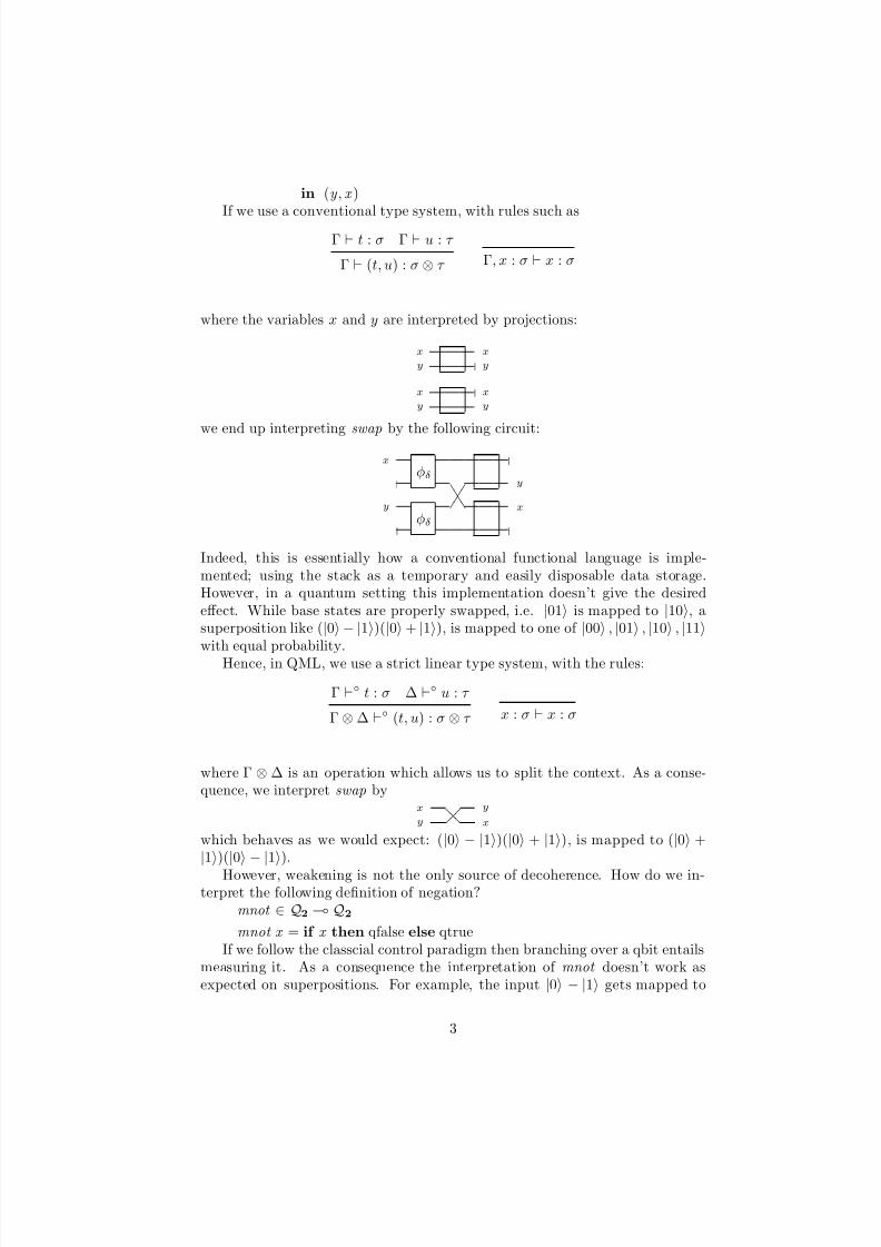
Next, we introduce a let-rule which is also the basic vehicle to define first

order programs. Γ a t : σ∆, x : σ a u : τ

letΓ ⊗ ∆ a let x = t in u : τ

By combining (let) and (emb) we can derive a more convenient scheme:

Γ a t : σ∆, x : σ b u : τ

Γ ⊗ ∆ ab let x = t in u : τ

where ◦ ◦ = ◦ and − otherwise.

Weakenings can affect the meaning of a program. As an example consider:

y : Q2 let x = y in x{} : Q2

This program will be interpreted as the identity circuit, in particular it isdecoherence-free. However, consider

y : Q2 let x = y in x{y} : Q2

This program uses weakening which will be interpreted as a measurement whichcauses decoherence.

2.2 Products (

⊗)

The rules for Q1, ⊗ are the standard rules from linear logic. In the case of Q1

instead of an explicit elimination rule we allow implicit weakening:

Q1 − intro• ◦ () : Q1

Γ, x : Q1 a t : σQ1 − weak

Γ a t : σ

Note that Q1 − weak preserves strictness, because no actual piece of informa-tion is eliminated. Using weakening we can derive non-strict version of theintroduction rule:

Γ ()domΓ : Q1

The product introduction rule is standard:

Γ a t : σ ∆ a u : τ ⊗ − intro

Γ ⊗ ∆ a (t, u) : σ ⊗ τ

7



The elimination rule is the usual pattern matching variant of the let-rule:

Γ a t : σ ⊗ τ ∆, x : σ, y : τ a u : ρ ⊗ − elim

Γ ⊗ ∆ a let (x, y) = t in u : ρ

As before for the let-rule, using (emb) we can derive

Γ a t : σ ⊗ τ ∆, x : σ, y : τ b u : ρ

Γ ⊗ ∆ ab let (x, y) = t in u : ρ

As an example, here is swap again:

p : Q2 ⊗ Q2 let (x, y) = p in (y{}, x{}) : Q2 ⊗ Q2

It is important to mark the variables with the empty set of variables. Thealternative program

p : Q2 ⊗ Q2 let (x, y) = p in (y{ p}, x{ p}) : Q2 ⊗ Q2

would measure the qbits while swapping them — this corresponds to the firstversion of swap in the introduction, based on the multiplicative rules.

2.3 Coproducts (⊕)

The introduction rules for ⊕ are the usual classical rules for +; note that theypreserve strictness.

Γ a s : σ⊕−intro1

Γ a inl s : σ ⊕ τ

Γ a t : τ ⊕−intro2

Γ a inr t : σ ⊕ τ

We define qbits Q2 = Q1 ⊕ Q1 and abbreviate qtrue x = qinl () x

and qfalsex =

qinr ()x

. We are not restricted to Q2 but can represent any finite type directly.As an example consider qtrits Q3 = Q1 ⊕ (Q1 ⊗ Q1) whose constructors 0, 1, 2can be defined anagolously to qtrue and qfalse.

As already indicated, we have two different elimination rules. We begin with

the one which measures a qbit, since it is basically the classical rule moduloadditivity of contexts.

Γ c : σ ⊕ τ ∆, x : σ t : ρ∆, y : τ u : ρ ⊕−elim

Γ ⊗ ∆ case c of {inl x ⇒ t | inr y ⇒ u} : ρ

8



We can derive if-then-else as

if b then t else u = case b of {inl ⇒ t | inr ⇒ u }and use this to implement a form of negation:mnot : Q2 Q2

mnot x = if x then qfalse else qtrueHowever, this program will measure the qbit before negating it. If we want toavoid this we have to use the decoherence-free version of case, which relies onthe orthogonality judgement: t ⊥ u, which is defined for terms in the same typeand context Γ t, u : A. We will introduce the rules for orthogonality later.Intuitively, t ⊥ u holds if the outputs t and u are always orthogonal, e.g. wewill be able to derive qtrue{} ⊥ qfalse{}. Hence, we introduce the strict caseby:

Γ a c : σ ⊕ τ

∆, x : σ ◦ t : ρ∆, y : τ ◦ u : ρ t ⊥ u ⊕−elim◦

Γ ⊗ ∆ a case◦ c of

{inl x ⇒ t | inr y ⇒ u} : ρ

Using the decoherence-free version if ◦ we can implement standard reversibleand hence quantum operations such as qnot :

qnot : Q2 Q2

qnot x = if ◦ x then qfalseelse qtrue

and the conditional not cnot:cnot : Q2 Q2 Q2 ⊗ Q2

cnot c x = if ◦ cthen (qtrue, qnot x )else (qfalse, x )

and finally the Toffolli operator which is basically a conditional cnot:toff : Q2 Q2 Q2 Q2 ⊗ (Q2 ⊗ Q2)

toff c x y = if ◦ cthen (qtrue, cnot x y )else (qfalse, (x , y ))

2.4 Superpositions

To be able to exploit quantum parallelism we have to be able to create superposi-tions like {qtrue | qfalse}, which is actually a shorthand for {( 1√

2)qtrue|( 1√

2)qfalse}.

Γ ◦ t, u : σ t ⊥ u|λ|2 + |λ|2 = 1

supΓ ◦ {(λ)t | (λ)u} : σ

9



As an example we can implement the Hadamard operator in QML:

had ∈ Q2

Q2

had x = if ◦ x then {(−1) qtrue | qfalse}else {qtrue | qfalse}

As already indicated earlier we omit the normalisation factors, which can beinferred. As we will see below the two alternatives are actually orthogonal,hence the the use of if ◦ is permitted.

If one of the coefficents is 0 it may be omitted, e.g. we write {(−1) qtrue} toconstruct a qbit which behaves like qtrue, if measured, but which has a differentphase. There is no need to introduce an n-ary superposition operator, since thiscan be simulated by nested uses of the binary operator, e.g.

{0 | 1 | 2} : Q3

can be encoded as

{(1

3

) 0|

( 2

3

){

1|

2}}

:Q3

2.5 Orthogonality

The idea of t ⊥ u is that we have an observation which tells the two terms apart.We will see that the information obtained by interpreting the derivations of this judgement is essential to compile case◦ and superpositions.

Different injections are orthogonal, we leave the typing premises for t, uimplicit:

Γ ◦ t : σ Γ ◦ u : τ Oinlr, Oinrl

inl t ⊥ inr u inr t ⊥ inl u

Constructors preserve orthogonality:

t ⊥ uOinl, Oinr

inl t ⊥ inl u inr t ⊥ inr u

t ⊥ uOpairl, Opairr

(t, v) ⊥ (u, w) (v, t) ⊥ (w, u)

Finally, superpositions can be orthogonal:

t ⊥ u λ∗0κ0 = −λ∗1κ1Osup

{(λ0)t | (λ1)u} ⊥ {(κ0)t | (κ1)u}

An instance of this rule is used when defining the Hadamard operator: wehave that

{(−1)qtrue|qfalse}|{qtrue|qfalse}which is just short for

{(− 1√2

)qtrue|( 1√2

)qfalse} ⊥ {(1√

2)qtrue|( 1√

2)qfalse}

10



The rules for orthogonality are incomplete, e.g. we never allow case◦-

expressions to be orthogonal, even though semantically this may be the case.Hence, we may in future add additional rules.

2.6 Programs

Programs are definitions of terms in contexts. We have omitted passing theprograms explicitely through the rules and also the requirement that the axiomsrequire that the program is well-typed. Well-typed programs can be constructedby the following obvious rule:

d d; Γ t : σdef

d, f Γ = t : σ

Note that unlike [Sel04], we do not allow any recursion. Previously definedfunctions can be used:

d = d, f (x1 : σ1,..,xn : σn) = t : τ d; Γ t1 : σ1, . . . tn : σnapp

d; Γ f t : τ

2.7 Examples

We present two small QML programs: a variant of Deutsch’s algorithm and anencoding of quantum teleportation in QML.

2.7.1 Deutsch’s algorithm

Deutsch’s algorithm is usually presented as the problem to find out whether aclassical function on Booleans is constant by querying the function only once.To avoid to have to resort to higher order, we solve here the morally equivalentproblem to decide whether two qbits, which are assumed to be classical, areequal, with the property that each branch of the program only queries one of the input bits. We arrive at the following QML program:

deutsch : Q2 Q2 Q2

deutsch a b = let (x , y ) = if ◦{qfalse | qtrue}then (qtrue, if ◦ a

then ({qfalse | (−1) qtrue}, (qtrue, b))else (

{(−

1) qfalse|

qtrue}

, (qfalse, b)))else (qfalse, if ◦ b

then ({(−1) qfalse | qtrue}, (a , qtrue))else ({qfalse | (−1) qtrue}, (a , qfalse)))

in had x We observe that the need to store both input qbits in the temporary structure

computed by if ◦ is actually unnecessary since we can assume that these bits are

11



classical and hence can be used without further measuring. If we had access to

classical bits we could simplify this program to:deutsch : 2 2 Q2

deutsch a b = let (x , y ) = if ◦{qfalse | qtrue}then (qtrue, if a

then {qfalse | (−1) qtrue}else {(−1) qfalse | qtrue}

else (qfalse, if bthen {(−1) qfalse | qtrue}else {qfalse | (−1) qtrue}

in had x We plan to incorporate classical bits in future versions of QML, very much

along the lines of Selinger’s QPL [Sel04].

2.7.2 Quantum teleportation

The quantum teleport protocoll allows us to teleport a qbit to a partner withwhom we share a EPR pair, using only two bits of classical information. Wecannot formalize the separation of the partners or their classical computationin QML, but we can implement a function tel , which encodes what happens tothe teleported qbit. The correctness of the teleport protocol can be verified byshowing that tel is extensionally equivalent to the identity function.

Auxilliary, we define Pauli’s Z-function:z : Q2 Q2

z x = if x then {(−1) qtrue} else qfalseand we implement tel as:

tel : Q2 Q2

tel x = let (a , b) = {(qfalse, qfalse), (qtrue, qtrue)}(a , x ) = cnot a x b = if a then qnot b else bb = if had x then z b else b

in b

3 Operational semantics

We define an operational semantics of QML by presenting a translation of QMLderivations to quantum computations representable as circuits. We will showthat the semantics doesn’t depend on the choice of derivations, but only on the

term up to extensional equality; introduced in the next section. We representirreversible computations as a reversible computation, which may use additionalquantum registers, or wires, which are initialised, and which can dispose of someregisters at the end of the computation. We have used this construction todefine the category of finite quantum computations, FQC [AG04]. Here we willuse the same notion for QML’s operational semantics, but we will not identifycomputations up to extensional equality here.

12



We use the size of a register, or equivalently the number of wires, as the types

of our computation. We use Q1 for 0 because it can represent just one state, andQ2 for 1, which is the type of qbits. We define a ⊗ b = a + b, because additionof wires corresponds to the tensor product in the structures we consider. Weidentify finite sets with natural numbers, i.e. any number a ∈ N is identifiedwith its initial segment, e.g. 2 = {0, 1}.

3.1 Reversible computations

We define the set if reversible quantum computations (or circuits) of size a ∈ N,FQC a inductively:

rotation rot u ∈ FQC Q2, where u ∈ 2 → 2 → C is a unitary matrix

u00 u01u10 u11

with u00u10 + u01u11 = 0. Note that negation qnot ∈ FQC Q2 is aspecial rotation given by qnot = rot unot where

unot =

0 11 0

wires wires φ ∈ FQC a where φ : a a is a bijection. This represents anyrewiring, including the identity ida = wires id

sequential composition Given φ ∈ FQC a and ψ ∈ FQC a we construct

φ ◦ ψ ∈ FQC a .

a ψ φ

parallel composition Given φ ∈ FQC a and ψ ∈ FQC b we constructφ ⊗ ψ : FQC (a ⊗ b).

a φ

b ψ

conditional Given φ, ψ

∈FQC a we construct φ

|ψ

∈FQC (

Q2

⊗a ).

In the literature the unary conditional is used. However, it is straightfor-ward to reduce our binary conditional to the usual unary:

Q2 • X • X

a ψ φ

13



To be able to interpret circuit diagrams unambiguously we assume that

(FQC, id, ◦, Q1, ⊗) is a strict monoidal category where FQC a a = FQC a and FQC a b = { }, if a ≡ b and that wires are a strict monoidal functor.That is, we consider FQC as a quotient — this could have been avoided byusing a notion of monoidal normal form, but this seems hardly relevant here.

In the literature, it is common to consider only a finite set of gates, this canbe achieved by using only a finite base of rotations from which any rotation canbe approximated, see [NC00], pp. 188.

3.2 Irreversible computations

Given a , b ∈ N standing for the size of inputs and output registers of the com-putation, a finite quantum computation α ∈ FQC a b is given by α = (h , g , φ)where

• h ∈ N is the size of the initial heap,

• g ∈ N is the size of the garbage to be disposed at the end of the compu-tation,

• c = a ⊗ h = b ⊗ g , otherwise we wouldn’t be able to find a reversiblecomputation,

• φ ∈ FQC c is a reversible computation.

This is different from our presentation of FQC in [AG04]: we only considerfinite sets of powers of 2, i.e. bit vectors, and we omit the heap initialisationvector, as a vector of 0’s is always used for the initialisation.

Diagrammatically, we represent such a computation as:

a b

φ 1

h g1

Note that, in the above diagram, heap inputs are initialised with a , andgarbage outputs are terminated with a .

Given a ∈ N we define ida = (Q1, Q1, ida) and the sequential compositionof computations α = (hα, gα, φα) ∈ FQC a b and β = (hβ , gβ , φβ ) ∈ FQC a b asβ ◦ α = (h,g,φ) ∈ FQC a c where

h = hα

⊗hβ

g = gα ⊗ gβ

φβ◦α = (gα ⊗ φβ ) ◦ (gβ ⊗ φα)

14



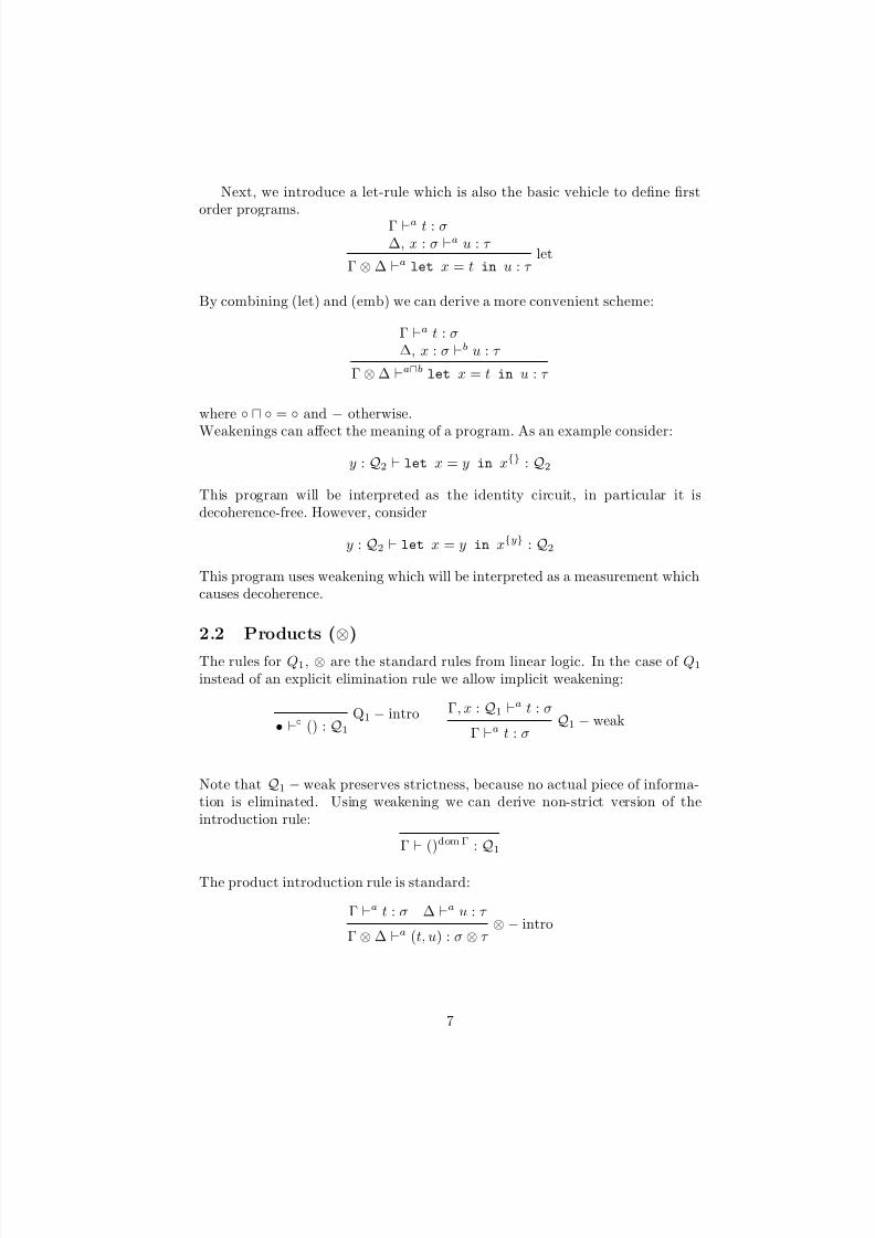
omitting some obvious monoidal isomorphisms from the definition of φβ◦α. Di-

agrammatically this construction is given by:a

φα

bφβ

c

hα 1

Y Y Y Y Y

V V V V V gα 1

hβ 1

Ó Ó Ó Ó Ó

Ö Ö Ö Ö Ö gβ 1

φβ◦α

We also define parallel composition for α ∈ FQC a b and β ∈ FQC c d asα ⊗ β = (h,g,φ) ∈ FQC (a ⊗ c) (b ⊗ d) where

h = hα ⊗ hβ

g = gα ⊗ gβ

φα

⊗β = φα

⊗φβ

again omotting monoidal isomorphisms. Diagrammatically, this is simply:

a

φα

b

c

V V V V V

V V V V V d

hα

Ö Ö Ö Ö Ö 1

φβ

Ö Ö Ö Ö Ö gα 1

hβ 1 gβ

1

φα⊗β

We notice that (FQC, id, ◦, Q1, ⊗) is a strict monoidal category. However,we will not exploit this fact but always construct FQC diagrams directly.

We define strict computations α = (h , φ) ∈ FQC◦ a b as one where g = Q1,

hence we are omitting it. We observe that this is a monoidal subcategory of FQC.

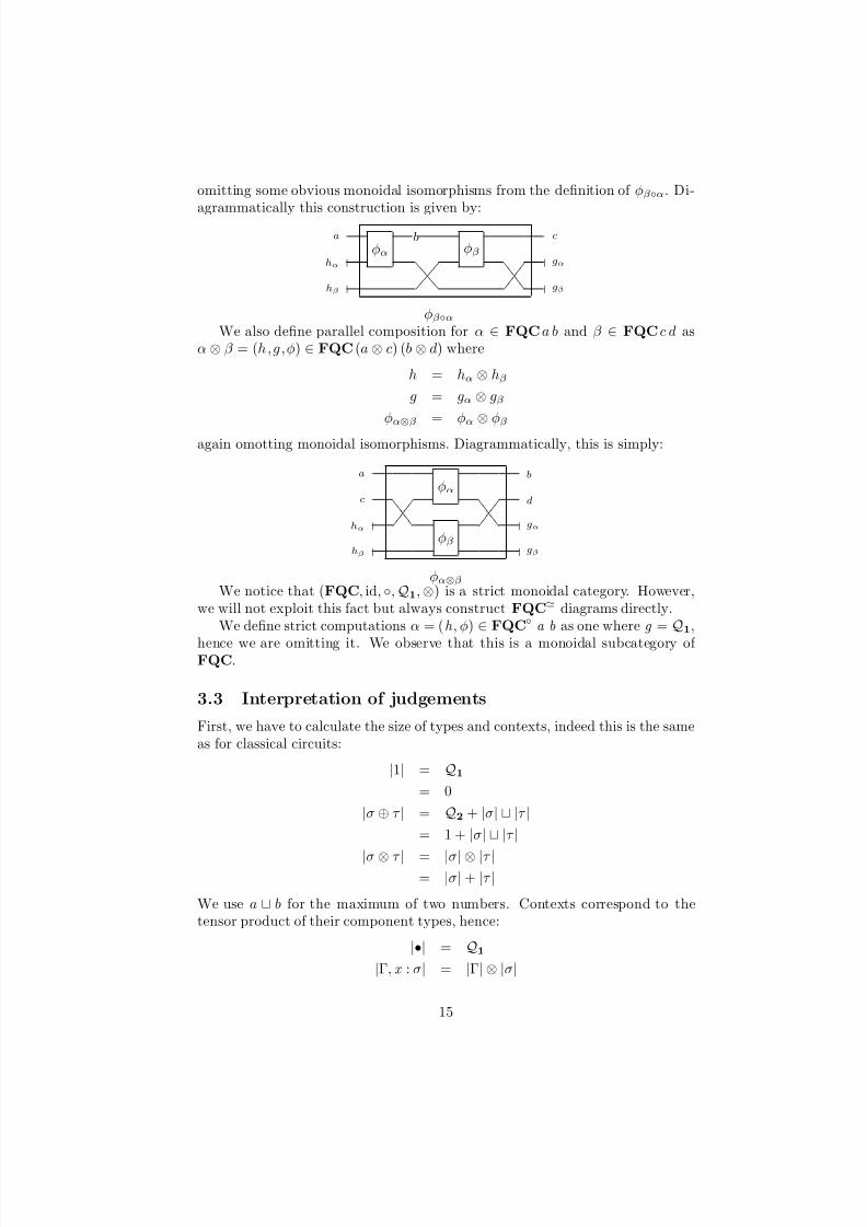
3.3 Interpretation of judgements

First, we have to calculate the size of types and contexts, indeed this is the sameas for classical circuits:

|1| = Q1

= 0

|σ ⊕ τ | = Q2 + |σ| |τ |= 1 + |σ| |τ |

|σ ⊗ τ | = |σ| ⊗ |τ |= |σ| + |τ |

We use a b for the maximum of two numbers. Contexts correspond to thetensor product of their component types, hence:

|•| = Q1

|Γ, x : σ| = |Γ| ⊗ |σ|

15



We will frequently omit the size function and just write Γ for |Γ| and σ for

|σ|. We interpret derivations

d

Γt:σ as d op ∈ FQC Γ σ and

d

Γot:σ as d op ∈FQC◦ Γ σ. Given Γ ◦ t : σ and Γ ◦ u : σ we interpret a derivation dt⊥u

as astructure d ⊥ = (c, l , r , ψ) where

• c ∈ N,

• l ∈ FQC◦ Γ c

• r ∈ FQC◦ Γ c

• ψ ∈ FQC σ (Q2 ⊗ c)

The semantics of programs d, is given by an assignement of circuits to functionnames. We will not study this in detail, since this it is straightforward andstandard.

3.4 Operations on contexts

Using Γ ⊗ ∆ we can use a variable several times, allowing contraction. Thisis interpreted using δ = (Q2, φδ) ∈ FQC◦ Q2 (Q2 ⊗ Q2) where φδ = id|qnot isconditional negation. First, we note that we can iterate δ to contract registersof any size: given a ∈ N we define δa ∈ FQC◦ a (a ⊗ a) by δ0 = wires id andδa⊗Q2 can be constructed from δa by

Q2 • Q2

a

G G G G G X G G G G G a

1

φδa

Q2

1a

Given Γ, ∆ such that Γ ⊗ ∆ is well-defined, we construct

CΓ,∆ ∈ FQC◦ |Γ ⊗ ∆| (|Γ| ⊗ |∆|)by induction over the definition of Γ ⊗ ∆. Note that the explicit use of |. . .| inthis formula is essential, since ⊗ is defined differently for contexts and for theirsize.

Γ, x : σ ⊗ ∆, x : σ = (Γ ⊗ ∆), x : σ

Γ⊗∆φC Γ,∆

Γ

σ

V V

V V

V V

V V σ Ö Ö Ö Ö 1

φδ σ

Ö Ö Ö Ö ∆

1σ

Γ, x : σ ⊗ ∆ = (Γ ⊗ ∆), x : σ, if x /∈ dom ∆

Γ⊗∆φC Γ,∆

Γ

σ V V V V

V V V V σ

hΓ,∆

Ö Ö Ö Ö 1 Ö Ö Ö Ö ∆

16



• ⊗ ∆ = ∆

•⊗∆ ∆

For the weakening rule we need an operator which forgets all variables whichonly occur in the second context, WΓ,∆ ∈ FQC |Γ ⊗ ∆| |Γ|. Again, this isdefined by induction over the definition of Γ ⊗ ∆: in the first two cases we have

Γ⊗∆φW Γ,∆

Γ

V V V V σ

σ

Ö Ö Ö Ö 1

and in the final case where, Γ is empty, we simply put ∆ into the garbage.

• ⊗ ∆ = ∆

•⊗∆ • 1

To interpret injections, it is necessary to increase the size of a morphismso it is the same size as another. To adjust the value of smaller size we use apadding operator Pσ,τ ∈ FQC◦ σ (σ τ ), which simply sets unused qbits to 0using extra heap space, equal to the difference.

σφP σ,τ

στ

hσ

.−τ

1

Here a .− b is cutoff subtraction, i.e. a .− b = a − b, if b a and 0, otherwise.

3.5 Structural rules

We present the compilation of rules using circuit diagrams. The interpretationof (emb) is invisible, since FQC◦ a b ⊆ FQC a b. Below are the circuits arisingfrom the variable and the weakening rule. (weak) uses the interpretation of its premise, we omit explicit references to h and g but refer to the reversiblecircuit φt arising from the interpretation of d

Γt:σand we will continue to use

this convention in the subsequent diagrams.

varx : σ ◦ x : σ

Γ t : σweak

Γ ⊗ ∆ tdom∆ : σ

σ σ Γ⊗∆φWΓ,∆

Γ

φt

σ

S S S S 1

1

Ù

Ù Ù Ù 1

Note that the variable rule is interpreted by a strict morphism. The let-rule isactually a scheme of two rules depending on a :

Γ a t : σ∆, x : σ a u : τ

letΓ ⊗ ∆ a let x = t in u : τ

17



Its circuit interpretation uses the copy circuit C and is uniform in a :

Γ⊗∆φC

Γ

W W W W ∆

φu 1

∆

Ö Ö Ö Öφt

σ τ

1

W W W W W Q Q Q Q 1

1 Ö Ö Ö Ö Ö

1

We notice that the result is strict, if both subderivations were strict.

3.6 Products (⊗)

The interpretation of the rules for Q1 in terms of circuits is invisible, since Q1

doesn’t carry any information. The interpretation of the rules for ⊗ is slightlymore interesting — the introduction rule simply merges the components:

Γ a t : σ ∆ a u : τ ⊗ − introΓ ⊗ ∆ a (t, u) : σ ⊗ τ

Γ⊗∆φC

Γ

φt

σ σ

1∆

W W W W U U U U U τ

1 Ö Ö Ö Ö Ö

φu

τ

× × × × 1

1 1

Using the fact that σ ⊗ τ is just interpreted by concatenating wires, the inter-pretation of the elimination rule is basically identical to the let-rule:

Γ

a t : σ⊗

τ ∆, x : σ, y : τ a u : ρ ⊗ − elim

Γ ⊗ ∆ a let (x, y) = t in u : ρ

Γ⊗∆φC

Γ

W W W W ∆

φu

1∆

Ö Ö Ö Ö

φt

σ

τ ρ

1

W W W W W Q Q Q Q 1

1 Ö Ö Ö Ö Ö

1

3.7 Coproducts (⊕)

As in classical computing, we represent values of σ ⊕ τ as a register which is bigenough to hold a value of either σ or τ and an extra bit for tagging. To adjustthe size of the value of smaller size we use the padding operator:

The introduction rules are compiled into circuits which pad and set the tagappropriately, we use σ τ to mark a quantum register which is large enough

18



to hold values of either type.

Γ a s : σ ⊕ intro1Γ a inl s : σ ⊕ τ

Γφs

σ

φPσ,τ 1 a a a a στ

1 Ñ Ñ Ñ Ñ

Q Q Q Q Q2

Q2 X 1

1

Γ a t : τ ⊕ intro2

Γ a inr t : σ ⊕ τ

Γ φt

τ

φPτ,σ 1

U U U U U στ

1 × × × ×

Q Q Q Q Q2Q2 1

1

We turn our attention to the two elimination operators: first the non-strict caserule

Γ c : σ ⊕ τ ∆, x : σ t : ρ∆, y : τ u : ρ ⊕ − elim

Γ ⊗ ∆ case c of {inl x ⇒ t | inr y ⇒ u} : ρ

We want to use the biconditional on the tagging qbit which arises from the

interpretation of the derivation of c. However, there is no reason, why thereversible computations arising from the derivations of t and u :

φt ∈ FQC st

φu ∈ FQC su

where

st = Γ ⊗ σ ⊗ ht

= ρ ⊗ gt

su = Γ ⊗ τ ⊗ hu

= ρ ⊗ gu

should have the same size. However, we can pad the smaller computation: Weobtain

ψt = φt ⊗ (su.− st)

∈ FQC (st su)

ψu = φt ⊗ (st.− su)

∈ FQC (st su)

19



We arrive at the following circuit:

Γ⊗∆φC

Γ

W W W W

ψt|ψu

1∆

Ö Ö Ö Ö

φc

σ τ ρ

Q2 Q2 1

1

g g g g g 1

1 { { { { { 1

Note that the non-strict case always introduce an extra qbit of garbage, whichis the qbit being measured.

To compile the strict case rule:

Γ a c : σ ⊕ τ ∆, x : σ ◦ t : ρ

∆, y : τ ◦ u : ρ t ⊥ u ⊕ − elim◦Γ ⊗ ∆ a case◦ c of

{inl x ⇒ t | inr y ⇒ u} : ρ

we have to exploit the data (d,l,r,ψt⊥u) which arises from interpreting theorthogonality judgement t ⊥ u. However, no further procrustenation is needed,because both φl, φr ∈ FQCd. We arrive at the following circuit:

Γ⊗∆φC

Γ

U U U

φl|φr

1∆

× × ×

φc

σ τ d

ψt⊥u

ρ

Q2 Q2

1

h h h h

1

{ { { { { 1

We observe that this rule preserve strictness, no garbage is added to the onealready produced by interpreting the derivation of c.

3.8 Superpositions

There is a simple syntactic translation we use to reduce the superposition op-erator to the problem of creating an arbitrary 1-qbit state:

Γ ◦ t, u : σ t ⊥ u|λ|2 + |λ|2 = 1 λ, λ = 0

Γ ◦ {(λ)t | (λ)u} : σ

≡if

◦ {(λ)qtrue

|(λ)qfalse

}then t else u

We can use our rotation primitive to produce any 1-qbit superposition simplyby rotating 0, the heap initialisation, to the intended position, i.e. we use

λ λ

λ −λ

20



Note that we have some freedom how to rotate the rest of the sphere, but any

choice is as good as any other.

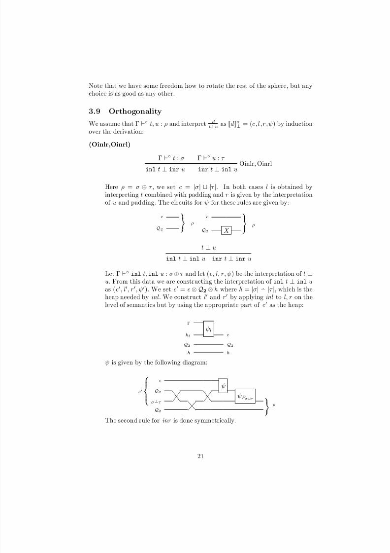
3.9 Orthogonality

We assume that Γ ◦ t, u : ρ and interpret dt⊥u

as d◦⊥ = (c,l,r,ψ) by inductionover the derivation:

(Oinlr,Oinrl)

Γ ◦ t : σ Γ ◦ u : τ Oinlr, Oinrl

inl t ⊥ inr u inr t ⊥ inl u

Here ρ = σ

⊕τ , we set c =

|σ

| |τ

|. In both cases l is obtained by

interpreting t combined with padding and r is given by the interpretationof u and padding. The circuits for ψ for these rules are given by:

c

Q2ρ

c

Q2 X ρ

t ⊥ u

inl t ⊥ inl u inr t ⊥ inr u

Let Γ ◦ inl t,inl u : σ ⊕ τ and let (c, l , r , ψ) be the interpretation of t ⊥u. From this data we are constructing the interpretation of inl t ⊥ inl u

as (c, l , r , ψ). We set c = c ⊗ Q2 ⊗ h where h = |σ|.− |τ |, which is the

heap needed by inl . We construct l and r by applying inl to l , r on thelevel of semantics but by using the appropriate part of c as the heap:

Γ

ψlhl c

Q2 Q2h h

ψ is given by the following diagram:

c

ψc Q2 U U U U U

U U U U UψP στ

σ.−τ

× × × × a a a a

× × × ×

Q2 Ñ Ñ Ñ Ñ

ρ

The second rule for inr is done symmetrically.

21



t

⊥u

(t, v) ⊥ (u, w) (v, t) ⊥ (w, u)

As above, let Γ ◦ (t, v), (u, w) : σ ⊗ τ and let (c,l,r,ψ) be the inter-pretation of t ⊥ u to construct the interpretation of (t, v) ⊥ (u, w) as(c, l, r, ψ). We set c = c ⊗ |τ | and construct l and r by pairing withv ,w , semantically:

Γ⊗∆φC

Γ

ψl

c

1∆

W W W W 1

Ö Ö Ö Ö Öψv

τ

1

The definition of ψ is given by the following diagram:

cψc

τ R R R R σ

Q2

τ ρ

t ⊥ u λ∗0κ0 = −λ∗1κ1

{(λ0)t | (λ1)u} ⊥ {(κ0)t | (κ1)u}

Let (c,l,r,ψ) be the interpretation of t

⊥u we construct the interpretation

of the conclusion as (c,l,r,ψ). We set c = c and define ψ ∈ FQCQ2 as

ψ =

λ0 λ1κ0 κ1

4 Denotational semantics

The denotational semantics of QML is based on a high level view of quantummechanics inspired by Selinger’s denotational semantics of QPL [Sel04]: wemodel finite-dimensional quantum states as vectors in a complex vector space,i.e. as functions from the finite classical state space to complex numbers. Wecan perform measurements on those states which have probabilistic outcomes

related to the complex amplitude and which collapses the part of the state whichis measured. Hence we require that the sum of probabilities of all possibleoutcomes of a measurement add up to 1. Reversible quantum computationscan be modelled by unitary operators, these are linear isomorphisms whichpreserve the probabilistic interpretation of amplitudes. Irreversible programs,involve measurements because we cannot dispose of a quantum bit withoutmeasuring it, and hence lead to mixed states, i.e. probabilistic distribution of

22



pure states. We use density operators to model mixed states and super operators

(aka completely positive operators) to interpret irreversible programs acting onpure states.

4.1 Linear algebra

In this section we review some basic notions from linear algebra. We also intro-duce the notation we use, which is based on functional programming idioms.

We use natural numbers as objects of the category of finite sets FinSetwhose homsets are given by FinSet a b = a → b, as before we identify naturalnumbers with their initial segements. Given a ∈ N we define C a = a → C.This function on objects C ∈ FinSet → Set is monadic, i.e. it gives rise to aKleisli structure, see [AR99], with

return

∈a

→C a

return a = λb → if a ≡ b then 1 else 0(>>=) ∈ (C a ) → (a → C b) → C bv >>= f = λb → Σ a .(v a )( f a b)

We are using an approximation to Haskell here, the proper definition is a bitmore involved, since we have to take into account that a, b are finite. See[VAS04] for a full development of superoperators as an instance of the arrowclass in Haskell.

The associated Kleisli category is the category of finite dimensional complexvector spaces FinVec, its homsets are given by FinVec a b = a → C b,where a , b ∈ N, and hence correspond to a × b complex matrices. Since we areworking with bit-vectors most of the time we define C2 a = C (2 → a ) andFinVec2 a b = FinVec (2 → a ) (2 → b).

The cartesian product on finite sets (the numeric product on natural num-bers) defines the tensor product on FinVec. I.e., on objects, a ⊗ b = ab; andon morphisms, given f ∈ FinVec a b, g ∈ FinVec c d we define f ⊗ g ∈FinVec (a ⊗ c) (b ⊗ d ) as f ⊗ g = λ(a , c) → λ(b, d ) → ( f a b)(g c d ). The unitof the tensor is I = 1, and (FinVec, ⊗, I ) is a strict monoidal category. Thetensor product in FinVec2 is given by +.

For vectors v , w ∈ C a we define their inner product v|w ∈ C as v|w =Σa.(va)

∗(w a ), where (x + yi )

∗= x − yi is the complex conjugate. The norm

of a vector v ∈ R+ is defined as v = v|v. Two vectors are orthogonal,v ⊥ w, if v|w = 0. A base of a vectorspace is orthonormal, if any two differentbase vectors are orthogonal.

Given f ∈ FinVec a b the adjoint of f is given by f † = λb a → ( f a b)∗

,with the defining property

v|f w

=

f †v

|w

. A map u

∈FinVec a b is unitary,

if its adjoint is its inverse u ◦ u† = id, this implies that u is an isomorphism,and hence also a = b. Unitary maps are isometric, i.e. they preserve the innerproduct, v|w = u v |u w . However, not all isometric maps are unitary, e.g.the diagonal maps δa ∈ FinVec a (a ⊗ a ), which are given by δ a (b, c) =if a ≡ b & b ≡ c then 1 else 0 are isometric but not unitary.

A linear map f ∈ FinVec a a is self-adjoint, if f = f †. A self-adjoint map

23



has only real eigenvalues; f v = λv implies λ ∈ R. The map is positive if all

eigenvalues are positive, that is λ

0. The trace of a map || f || is the sum of alleigenvalues, which can be directly calculated as || f || = Σ a . f a a .

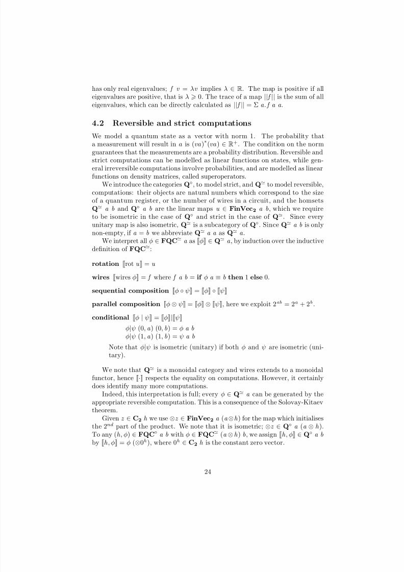
4.2 Reversible and strict computations

We model a quantum state as a vector with norm 1. The probability thata measurement will result in a is (va)

∗(va) ∈ R+. The condition on the norm

guarantees that the measurements are a probability distribution. Reversible andstrict computations can be modelled as linear functions on states, while gen-eral irreversible computations involve probabilities, and are modelled as linearfunctions on density matrices, called superoperators.

We introduce the categories Q◦, to model strict, and Q to model reversible,computations: their objects are natural numbers which correspond to the size

of a quantum register, or the number of wires in a circuit, and the homsetsQ a b and Q◦ a b are the linear maps u ∈ FinVec2 a b, which we requireto be isometric in the case of Q◦ and strict in the case of Q. Since everyunitary map is also isometric, Q is a subcategory of Q◦. Since Q a b is onlynon-empty, if a = b we abbreviate Q a a as Q a .

We interpret all φ ∈ FQC a as φ ∈ Q a , by induction over the inductivedefinition of FQC:

rotation rot u = u

wires wires φ = f where f a b = if φ a ≡ b then 1 else 0.

sequential composition φ ◦ ψ = φ ◦ ψ

parallel composition φ ⊗ ψ = φ ⊗ ψ, here we exploit 2ab = 2a + 2b .

conditional φ | ψ = φ|ψ

φ|ψ (0, a ) (0, b) = φ a bφ|ψ (1, a ) (1, b) = ψ a b

Note that φ|ψ is isometric (unitary) if both φ and ψ are isometric (uni-tary).

We note that Q is a monoidal category and wires extends to a monoidalfunctor, hence · respects the equality on computations. However, it certainlydoes identify many more computations.

Indeed, this interpretation is full; every φ

∈Q a can be generated by the

appropriate reversible computation. This is a consequence of the Solovay-Kitaevtheorem.

Given z ∈ C2 h we use ⊗z ∈ FinVec2 a (a ⊗h ) for the map which initialisesthe 2nd part of the product. We note that it is isometric; ⊗z ∈ Q◦ a (a ⊗ h ).To any (h , φ) ∈ FQC◦ a b with φ ∈ FQC (a ⊗ h ) b, we assign h , φ ∈ Q◦ a bby h , φ = φ (⊗0h ), where 0h ∈ C2 h is the constant zero vector.

24



For orthogonal maps, that is f , g ∈ Q◦ a b such that for all a ∈ C2 a we

have f ⊥ g we can define another form of the conditional f |◦g ∈ Q◦ (Q2 ⊗ a ) bas f |◦g (0, a ) b = f a b f |◦g (1, a ) b = g a b

Clearly, we have f |g = 0 ⊗ f |◦1 ⊗ g .

4.3 Irreversible computations

To interpret irreversible computations we have to model mixed states, whicharise as the result of a measurement. A mixed state of size a is represented asa positive map ρ ∈ FinVec2 a a , such that ||ρ|| = 1. This is called a densitymatrix. The idea is that the probability that ρ is in state v is λ, if ρ v = λv ,i.e. v is an eigenvector with eigenvalue λ, and 0 otherwise. The trace condition

ensures that this is a probability distribution on the vectors in any orthonormalbase.

A linear map f ∈ FinVec2 (a ⊗ a ) (b ⊗ b) can be interpreted as an operatoron density matrices by using that FinVec2 a a C2 (a ⊗ a ) 2 . We say thatsuch an operator is positive if it preserves positivity. It is completely positiveif f ⊗ (c ⊗ c) ∈ FinVec2 ((a ⊗ c) ⊗ (a ⊗ c)) ((b ⊗ c) ⊗ (b ⊗ c)), is positivefor any c ∈ N. It is a superoperator if it is completely positive, and trace-preserving. We define Q as the category of superoperators, i.e. its objectsare natural numbers and its morphisms are superoperators, that is Q a b isgiven by f ∈ FinVec2 (a ⊗ a ) (b ⊗ b), which are completely positive andnorm-preserving. The tensor product on super operators is given by the tensorproduct of the underlying vector space.

Isometric maps give rise to superoperators. Given f ∈ Q◦ a b, we define f ∈ Q a b as follows: given a density matrix ρ ∈ FinVec2 a a , we construct f ρ = f ◦ρ◦( f †) ∈ FinVec2 b b, using the isomorphism FinVec a a C (a ⊗a ).This gives rise to f ∈ FinVec2 (a ⊗ a ) (b ⊗ b), which is completely positive andtrace preserving.

We interpret measurements as partial trace, defining Trab ∈ Q (a ⊗ b) a asTrab ∈ FinVec2 ((a ⊗ b) ⊗ (a ⊗ b)) (a ⊗ a )

Trab = λ(a , b) (a , b) → if b ≡ b

then return (a , a )else λ( , ) → 0

It can be verified that Trab is completely positive and norm preserving.Given the above, we can interpret (h , g , φ) ∈ FQC a b as (h , g , φ)FQC ∈

Q a b using (h , φ)◦

∈Q◦ a (b

⊗g ), which can be embedded in FQC:

(h , φ◦FQC) ∈ Q a (b ⊗ g ) and finally using the partial trace, we obtain

(h , g , φ)FQC ∈ Q a b

(h , g , φ)FQC = Trbg (((h , φ)))

2Correct would be C2 (a⊥ ⊗ a), but since our objects are natural numbers, this doesn’treally matter.

25



We can use Kraus’ representation theorem to show that this interpretation is

full, i.e. all superoperators can be realised by an FQC-morphism.To see that ·FQC is actually functorial, we have to show that the compo-sition in FQC as defined in section 3.2 is preserved by ·.

Proposition 1 · ∈ FQC → Q is a strict monoidal functor, that is

1. id = id

2. f ◦ g = f ◦ g

3. f ⊗ g = f ⊗ g

Proof: Both 1. and 3. follow directly from monoidal identities. The onlyinteresting case is 2. which follows from the fact that the following diagram

commutes:

a⊗ hf ⊗ hg

φf⊗hg / / b⊗ gf ⊗ hg

φg⊗gf / /

trgf

U U U U U U U U U U U U U U Uc⊗ gf ⊗ gg

trgfgg

" " i i i i i i i i

trgg

a

zf⊗zg < < x x x x x x x x

zf " " p p p p p p p p c

a⊗ hf φf

/ /

zg

O O

b⊗ gf trgf

/ /

zg

C C × × × × × × × × × × × × × × ×b zg

/ / b⊗ hgφg

/ / c⊗ gg

trgg

< < y y y y y y y y

By combining the operational semantics and the denotational semantics of

computations we obtain an interpretation of derivations as isometric maps orsuperoperators, that is given a derivation of dΓt:σ

we get d ∈ Q Γ σ by

d = d opFQC and given dΓ◦t:σ

we get d ◦ ∈ Q◦ Γ σ by d = d ◦op◦FQC.

5 Conclusions and further work

We have introduced a language for finite quantum programs which featuresquantum control and quantum data. We have identified the fact that weaken-ings affect the behaviour of a quantum program as one of the main structuraldifferences between quantum and classical programming, and consequently usea strict linear type system where weakenings are explicit. The fact that for-getting information may affect other parts of the computation also necessitates

the orthogonality judgement, which witnesses the fact that our quantum controloperator case◦ does not irreversibly disposes information.

We have given an operational semantics of the language in terms of reversiblequantum circuits. These circuits can model irreversible computation by havingaccess to initialised heap registers at the start of the computation, which disopseunusued data at the end. The operational semantics has been implemented byGrattage in Haskell, [GA05].

26



We also present a denotational semantics by interpreting the circuits arising

from the operational semantics by superoperators — here we draw heavily onSelinger’s work on QPL [Sel04].The present paper is an extended version of our conference submission

[AG04]. We also have tried to improve and reorganise the presentation byclearly separating operational and denotational semantics: While in [AG04] wecollapsed morphisms in FQC upto extensional equality, we now only identifycomputations upto monoidal identities (upto isomorphic circuit diagrams), andleave the extensional equality to the denotational model, i.e. to the category Q.

Much remains to be done, which we have left out of the current paper forreasons of space and time: to show the denotational semantics is derivationindependent, i.e. different typing derivations of the same term do not affect itsinterpretation upto extensional equality; and is also compositional, i.e. replacingextensionally equivalent subterms results in extensionally equivalent programs.

To show derivation independence, we observe that most of the rules arestructural with the exception of (emb) and (⊕−elim◦). (emb) doesn’t causeany problems since it is interpreted by FQC◦ a b ⊆ FQC a b in the operationalsemantics. (⊕−elim◦) is more interesting: we need to show that the interpre-tation of t ⊥ u is semantically correct, i.e. that the interpretation of the termscan be obtained by composing the corresponding component of the orthogo-nality judgement with the unitary map ψ; that t = ψ−1 ◦ (qtrue ⊗ l) andu = ψ−1 ◦ (qfalse⊗ r). We can use this to show that the interpretation of (⊕−elim◦) does not depend on the derivation of orthogonality.

To show compositionality, it seems that the best way is to directly give anintepretation of QML programs in Q and then show that this interpretationfactors through the operational semantics. This denotational semantics can be

effectively computed, we plan to use the material in [VAS04] to implement thesemantics in Haskell. In many cases compositionality follows from proposition 1and the observation that we only use horizontal (◦) and vertical (⊗) compositionto define the interpretation of terms from their components. The only exceptionsare the elimination rules for ⊕: In the case of (⊕−elim◦) we have to show that f |◦g comutes with initialisations. (⊕−elim) is slightly more involved since wealso have to commute the partial traces. Indeed, this only works because wemeasure the qbit we are branching over.

More tentative is the extension of QML to higher types, and being able toincorporate infinite data structures.

Q doesn’t seem to have a closed structure which would allow us to interprethigher order programs (see [?] for a discussion). However, this is not reallynecessary since we are only running higher order programs once they are fully

applied. Semantically, this observation can be exploited by interpreting higherorder programs in the presheaf category over Q, which has a tensor productby Day’s construction and is automatically closed with respect to this tensorproduct. There is no clear candidate for ⊕, and, since it is not at all obvioushow a coproduct of higher order quantum functions may be implemented, thebest choice may be not to allow this, but to limit ⊕ to first order types.

Infinite data structures could be interpreted in infinite-dimensional vector

27



spaces using the standard approaches from mathematical physics. An alterna-

tive, which is closer to potential implementations of quantum programs, is toallow quantum programs to be indexed by classical structures in a way akinto Dependent ML (DML) [?]. DML is a language with dependent types whereindex expressions and actual programs are clearly separated. In the case of DML, this separation is needed to deal with impurities in the actual programs,such as non-termination. In a dependently typed version of QML, the sameapproach would be used to separate the classical structure of the computationfrom quantum effects.

Finally, having a high level language with a clear semantics should lead toreasoning principles which could be expressed as an algebra of quantum pro-gramming. This algebra should enable us to give mathematically clear, formalcorrectness proofs of quantum programs. This algebra is related to Tondersquantum λ calculus, [vT03b], but we would aim to include measurements and

justify the equations by showing that they are sound and complete with respectto the denotational semantics in Q.

Acknowledgements

We would like to thank our colleagues and friends Slava Belavkin, Bob Coecke,Martin Hofmann, Graham Hutton, Conor McBride, Amr Sabry, Peter Selinger,Alex Simpson, Thomas Streicher, Janine Swarbrick and Juliana Vizotti for in-teresting discussions and feedback on our work. Amr Sabry and Juliana Vizottiprovided extensive feedback on previous drafts of this paper. Peter Selingerpointed out a serious flaw in an earlier version of case◦ and refuted our conjec-ture that strict maps classify monos in Q.

References

[AD04] P. Arrighi and G. Dowek. Operational semantics for a formal tensorialcalculus, 2004. Draft proceedings of the 2nd International Workshopon Quantum Programming Languages.

[AG04] T. Altenkirch and J. Grattage. A functional quantum programminglanguage. quant-ph/0409065, November 2004.

[AR99] T. Altenkirch and B. Reus. Monadic presentations of lambda termsusing generalized inductive types. In Computer Science Logic, 1999.

[GA05] J. Grattage and T. Altenkirch. A compiler for a functional quantumprogramming language. Submitted for publication, January 2005.

[Gru99] J. Gruska. Quantum Computing . McGraw-Hill, Maidenhead, 1999.

[Hir01] M. Hirvensalo. Quantum Computating . Springer-Verlag NewYork, Inc.,2001.

28



[Hug00] J. Hughes. Generalising monads to arrows. Sci. Comput. Program.,

37(1-3):67–111, 2000.[Kar03] J. Karczmarczuk. Structure and interpretation of quantum mechan-

ics: a functional framework. In Proceedings of the ACM SIGPLAN workshop on Haskell , pages 50–61. ACM Press, 2003.

[Kni96] E. Knill. Conventions for quantum pseudocode, 1996.

[MB01] S-C. Mu and R. S. Bird. Quantum functional programming. In 2nd Asian Workshop on Programming Languages and Systems, 2001.

[NC00] M. Nielsen and I. Chuang. Quantum Computation and Quantum In- formation . Cambridge University Press, Cambridge, 2000.

[Ome03] B. Omer. Structured Quantum Programming . PhD thesis, Institutefor Theoretical Physics, Technical University of Vienna, Vienna, 2003.

[Pit00] A. Pittenger. An Introduction to Quantum Computing Algorithms,volume 19 of Progress in Computer Science and Applied Logic (PCS).Berkhauser, 2000.

[Pre99] J. Preskill. Quantum computation course lecture notes, 1999.

[Sab03] A. Sabry. Modeling quantum computing in haskell. In Proceedings of the ACM SIGPLAN workshop on Haskell , pages 39–49. ACM Press,2003.

[Sel04a] P. Selinger. Towards a quantum programming language. Mathematical

Structures in Computer Science, 2004.[Sel04b] P. Selinger. Towards a semantics for higher-order quantum computa-

tion. Draft proceedings of the 2nd International Workshop on Quantum Programming Languages, 2004.

[SV05] P. Selinger and B. Valiron. A lambda calculus for quantum computa-tion with classical control. To appear in the proceedings of TLCA05,2005.

[SZ00] J. Sanders and P. Zuliani. Quantum programming. In Mathematicsof Program Construction , volume 1837 of Springer Lecture Notes in Computer Science, pages 80–99. Springer-Verlag, 2000.

[VAS04] J. K. Vizzotto, T. Altenkirch, and A. Sabry. Structuring quantumeffects: Superoperators as arrows. Submitted for publication, 2004.

[vT03a] A. van Tonder. A lambda calculus for quantum computation. quant-ph/0307150, 2003. to appear in SIAM Journal of Computing.

[vT03b] A. van Tonder. Quantum computation, categorical semantics and lin-ear logic. quant-ph/0312174, 2003.

29



[Xi98] H. Xi. Dependent Types in Practical Programming . PhD thesis,

Carnegie Mellon University, 1998.

30

Thorsten Altenkirch and Jonathan Grattage- QML: Quantum data and control

Documents

Transcript of Thorsten Altenkirch and Jonathan Grattage- QML: Quantum data and control