Thoracic Artificial Lung Design

by

Rebecca E. Schewe-Mott

A dissertation submitted in partial fulfillment of the requirements for the degree of

Doctor of Philosophy (Biomedical Engineering)

in the University of Michigan 2012

Doctoral Committee: Associate Research Professor Keith E. Cook, Chair Professor Emeritus Robert Hawes Bartlett Associate Professor Joseph L. Bull

Assistant Research Scientist Khalil M. Khanafer

© Rebecca E. Schewe-Mott 2012

ii

Acknowledgements

I would like to thank my committee for all of their guidance and support

throughout this process. You have each contributed to my learning and the development

of this project. I especially want to thank my advisor, Keith Cook, for everything he has

taught me. Keith has been incredibly supportive, encouraging, and an amazing resource

for this work.

I would also like to thank all of the students and surgical staff that worked on this

project. The fabrication process for the cTALs was developed over many years by many

different students. Ryan Orizondo started this work with me and without him our

fabrication process would not be what it is today. Kelly Koch worked extremely hard as

the lab technician on all the acute and chronic animal studies presented in this work.

Chris Scipione performed all the surgeries, monitoring of the animals, and helped me

perform all the animal experiments presented in this thesis. Chris was a great resource for

me and without his and Kelly’s hard work the animal experiments wouldn’t have been

possible. I also want to thank all of my fellow graduate students and lab mates. I have

enjoyed working with all of you and appreciate your help and guidance over the years.

I finally want to thank my family and friends for their unwavering love and

support. Without you, I may never have finished this dissertation.

iii

Table of Contents

Acknowledgements ............................................................................................................. ii  

List of Figures .................................................................................................................. viii 

List of Tables ................................................................................................................... xiv 

ABSTRACT ...................................................................................................................... xv 

Chapter 1: Introduction ....................................................................................................... 1 

Motivations and Objectives ............................................................................................ 1 

Lung Disease and Transplantation .................................................................................. 2 

Respiratory Support Options ........................................................................................... 3 

Thoracic Artificial Lung Development ......................................................................... 15 

Compliant TAL ............................................................................................................. 21 

Summary of the Study .................................................................................................. 22 

References ..................................................................................................................... 24 

Chapter 2: Thoracic Artificial Lung Housing Design ....................................................... 30 

Introduction ................................................................................................................... 30 

Methods......................................................................................................................... 31 

Computational Fluid Dynamics Studies ................................................................... 31 

iv

CFD: Problem Formulation ...................................................................................... 32 

CFD: Boundary Conditions ...................................................................................... 33 

CFD: Numerical Scheme .......................................................................................... 36 

CFD: Data Analysis .................................................................................................. 36 

In Vitro Testing ......................................................................................................... 39 

Results ........................................................................................................................... 41 

CFD: Rigid Housing TAL ........................................................................................ 41 

Discussion ..................................................................................................................... 51 

References ..................................................................................................................... 56 

Chapter 3: Compliant Thoracic Artificial Lung Design and Testing ............................... 58 

Introduction ................................................................................................................... 58 

Methods......................................................................................................................... 59 

Fluid Structure Interaction Analysis ......................................................................... 59 

FSI: Problem Formulation ........................................................................................ 59 

FSI: Numerical Scheme ............................................................................................ 62 

FSI: Data Analysis .................................................................................................... 62 

Compliant Thoracic Artificial Lung ......................................................................... 63 

In Vitro Testing: Hemodynamics .............................................................................. 64 

In Vitro Testing: Gas Transfer .................................................................................. 66 

Results ........................................................................................................................... 67 

v

Fluid Structure Interaction Analysis ......................................................................... 67 

In Vitro Testing: Hemodynamics .............................................................................. 72 

In Vitro Testing: Gas Transfer .................................................................................. 74 

Discussion ..................................................................................................................... 75 

References ..................................................................................................................... 82 

Chapter 4: In-Parallel cTAL Attachment .......................................................................... 83 

Introduction ................................................................................................................... 83 

Methods......................................................................................................................... 84 

Compliant Thoracic Artificial Lung ......................................................................... 84 

Experimental Procedure ............................................................................................ 84 

Data Analysis ............................................................................................................ 87 

Results ........................................................................................................................... 88 

Animal Physiology.................................................................................................... 88 

Device Performance .................................................................................................. 92 

Discussion ..................................................................................................................... 94 

Conclusion ................................................................................................................ 98 

Chapter 5: In-Series cTAL Attachment .......................................................................... 101 

Introduction ................................................................................................................. 101 

Methods....................................................................................................................... 102 

Experimental Procedure .......................................................................................... 102 

vi

Data Analysis .......................................................................................................... 105 

Results ......................................................................................................................... 107 

Animal Physiology.................................................................................................. 107 

Device Function ...................................................................................................... 115 

Discussion ................................................................................................................... 116 

References ................................................................................................................... 118 

Chapter 6: Conclusion..................................................................................................... 119 

Conclusions ................................................................................................................. 119 

Limitations and Future Work ...................................................................................... 121 

Appendix: Compliant Thoracic Artificial Lung Fabrication .......................................... 125 

Summary ..................................................................................................................... 125 

Dipping: Creating the cTAL Housing......................................................................... 126 

Percent Solid ........................................................................................................... 126 

Day 1 – Dipping the Proximal End of the Device (All Pieces Separate) ............... 128 

Day 2 – Dipping the Proximal End of the Device (All Pieces Assembled) ........... 132 

Day 3 – Dipping the Distal End of the Device ....................................................... 134 

Day 4 – Laying the Bead ........................................................................................ 136 

Day 5 – Water Submersion ..................................................................................... 137 

Day 6 – De-molding................................................................................................ 137 

Leak Testing and Patching: Housing .......................................................................... 138 

vii

Leak Testing Housing ............................................................................................. 138 

Patching Housing with Biospan .............................................................................. 140 

Rolling Fiber Bundles ................................................................................................. 140 

Making the Core for the Fiber Bundle .................................................................... 141 

Wrapping the Fiber ................................................................................................. 142 

Potting: Binding the cTAL fiber bundle and housing ................................................. 145 

Preparing Devices for Potting ................................................................................. 145 

Preparing Centrifuge ............................................................................................... 146 

Preparing Potting Material ...................................................................................... 147 

Potting Procedure .................................................................................................... 148 

Cutting: Exposing the ends of the fibers ..................................................................... 150 

Leak Testing and Patching: Potted and Cut Devices .................................................. 153 

Leak Testing Cut Devices: ...................................................................................... 153 

Patching Cut Devices: Housing .............................................................................. 154 

Patching Cut Devices: Potting ................................................................................ 154 

Attaching Gas Caps and Performing Air Leak Tests .................................................. 155 

viii

List of Figures

Figure 1.1: Illustration of a patient on a mechanical ventilator. ......................................... 4 

Figure 1.2: Standard V-A ECMO circuit. Blood is removed from the right atrium, into a

venous reservoir, and then through a pump. The blood is pumped through a membrane

oxygenator, heat exchanger, and then returned to the arterial circulation. Heparin and

other fluids are given through this circuit. ECMO system. 29 Mar, 2011. Medscape

Reference. Web. 11 Mar 2012. ........................................................................................... 6 

Figure 1.3: Arterio-venous CO2 removal circuit. Blood flows from a cannula inserted in

the femoral artery, through a membrane oxygenator where gas exchange occurs, and then

back to the patient through a cannula inserted in the femoral vein. ................................... 8 

Figure 1.4: Novalung iLA. Spillner J et al. Frontiers in Bioscience 16: 2342-2351, 2011 9 

Figure 1.5: (a) Picture of the IVOX in its unfurled state and (b) cross-sectional schematic

of the IVOX, showing the gas flow path through the device. Kallis et al. Eur J of

Cardiothorac Surg 7(4): 206-210, 1993. .......................................................................... 11 

Figure 1.6: Highly integrated intravascular membrane oxygenator (HIMOX) utilizing a

series of disc-shaped fiber bundles along a core and an axial blood pump. Cattaneo et al.

ASAIO J 52:180-5, 2006. .................................................................................................. 11 

ix

Figure 1.7: Schematic of the intravenous respiratory assist catheter, consisting of a

pulsating balloon surrounding by a bundle of hollow fibers. Federspiel et al. ASAIO J

42:M435-42, 1996............................................................................................................. 12 

Figure 1.8: Schematic of the paracorporeal assist lung (PRAL) which utilizes a rotating

fiber bundle to enhance gas exchange. Svitek et al. ASAIO J 51(6): 773-80, 2005. ........ 13 

Figure 1.9: Cross-sectional view of the artificial pump lung (APL) showing the blood

flow path. Wu et al. Ann Thorac Surg 93:274-81, 2012................................................... 15 

Figure 1.10: TAL attachment (a) in parallel (PA-LA) and (b) in series (PA-PA) ............ 16 

Figure 1.11: Blood flow path through the MC3 Biolung.................................................. 17 

Figure 1.12: Biolung with a polyurethane compliance chamber attached to its inlet.

McGillicuddy et al. ASAIO J 51:789-794, 2005. .............................................................. 19 

Figure 1.13: Original cTAL prototype, consisting of a compliant Biospan housing and

fiber bundle. Cook et al. ASAIO J 51: 404-411, 2005. ..................................................... 21 

Figure 1.14: Inlet and outlet expansion angle, θ, of the cTAL inlet and outlet housing

manifolds........................................................................................................................... 22 

Figure 1.15: cTAL models with θ=15, 45, and 90° .......................................................... 22 

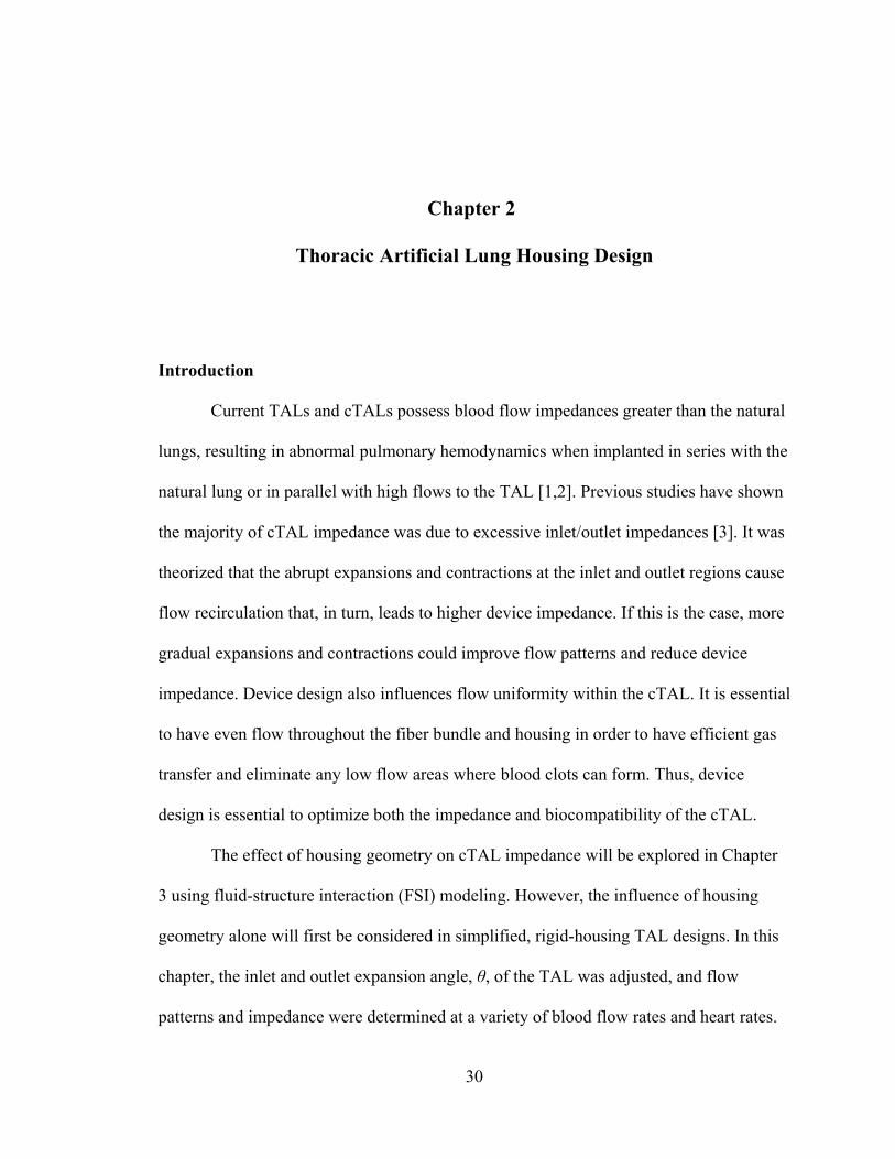
Figure 2.1: TAL model showing blood flow path and inlet and outlet expansion angle, θ

........................................................................................................................................... 31 

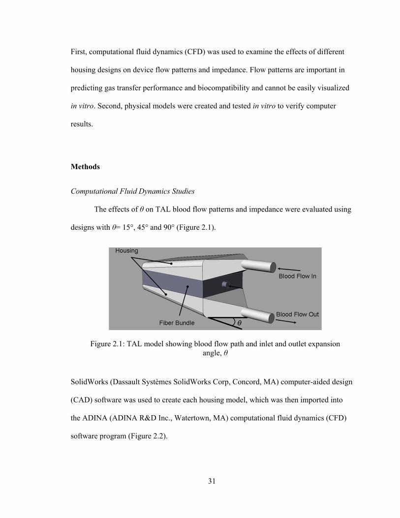
Figure 2.2: TAL housing models used for CFD study with θ = 15°, 45° and 90° ............ 32 

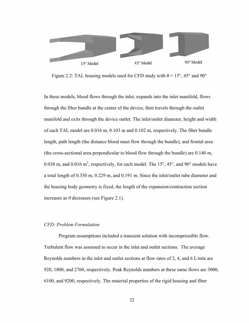
Figure 2.3: TAL inlet flow waveform for CFD and in vitro studies at 4 L/min, 100

beats/min, and pulsatilities of 2 and 3.75. ......................................................................... 34 

x

Figure 2.4: In vitro test circuit consisting of a pulsatile pump, TAL model, and reservoir

filled with 3.0 cP glycerol solution. Six pressure lines were connected to the model at the

inlet (P1), outlet (P2), top of the bundle (P3 and P5), and bottom of the bundle (P4 and

P6). .................................................................................................................................... 39 

Figure 2.5: Effect of θ on TAL Z0 for varying stroke volumes: comparison between in

vitro and CFD results ........................................................................................................ 41 

Figure 2.6: Effect of θ on TAL Z1 for varying heart and flow rates: CFD results ............ 42 

Figure 2.7: Velocity band plots for the 15° and 90° CFD TAL models at a pulsatility of

3.75 and the 45° model at a pulsatility of 3.75 and 2. Shown at peak systole in the (a)

inlet housing region and (b) fiber bundle .......................................................................... 44 

Figure 2.8: Velocity band plots for the 15° and 90° CFD TAL models at a pulsatility of

3.75 and the 45° model at a pulsatility of 3.75 and 2. Shown at end-diastole for two

different velocity plot ranges. ........................................................................................... 45 

Figure 2.9: (a) Velocity vector plots for the 15°, 45°, and 90° CFD TAL models at the

beginning of diastole (t=1.58s) in the inlet housing region. (b) Magnified view of the

major recirculation areas in each model. .......................................................................... 46 

Figure 2.10: (a) Velocity vector plot for the 90° TAL model during peak systole (t=1.32s)

in the inlet housing region. Magnified view of the major recirculation areas located in the

(b) proximal end of the housing and (c) distal end of the device. .................................... 47 

Figure 2.11: Velocity vector plots for the 15° and 90° CFD TAL models at a pulsatility of

3.75 and the 45° model at a pulsatility of 3.75 and 2. Shown at end-diastole in the inlet

housing region. .................................................................................................................. 48 

xi

Figure 2.12: (a) Velocity vector plot for the 45° TAL model at the beginning of diastole

(t=1.58s) in the outlet housing region. Magnified view of the outlet tube (b) and the

proximal end of the housing (c) showing small recirculation regions. ............................. 49 

Figure 2.13: Effect of θ on TAL Z1: comparison between in vitro and CFD results for

varying heart and flow rates .............................................................................................. 50 

Figure 3.1: cTAL prototype showing blood flow path ..................................................... 63 

Figure 3.2: (a) In vitro testing circuit for resistance study consisting of pulsatile pump,

cTAL, and reservoir filled with 3.0 cP glycerol solution. Two pressure lines were

connected to the model at the inlet (P1) and outlet (P2). (b) Gas transfer testing circuit

consisting of a reservoir filled with bovine blood, roller pump, deoxygenator

(conditioning loop) and a cTAL (testing loop). ................................................................ 65 

Figure 3.3: cTAL inlet and outlet flow waveforms for the FSI models at 3 L/min and 100

beats/min, showing outlet flow dampening. Representative cTAL inlet flow waveform

from the in vitro study at 4 L/min and 100 beats/min. ...................................................... 67 

Figure 3.4: FSI results showing the effect of θ on cTAL Z0 and Z1 for varying stroke

volumes ............................................................................................................................. 68 

Figure 3.5: (a) Velocity vector plots for the 15°, 45°, and 90° cTAL models at the

beginning of diastole (t=2.14s) in the inlet housing region. (b) Magnified view of the

major recirculation areas in each model. .......................................................................... 69 

Figure 3.6: Velocity band plots for the 15°, 45°, and 90° cTAL models at peak systole in

the (a) inlet housing region at the entrance to the fiber bundle and (b) middle of the fiber

bundle ................................................................................................................................ 70 

xii

Figure 3.7: Flow waveforms entering the fiber bundle for the 15°, 45°, and 90° cTAL

models ............................................................................................................................... 71 

Figure 3.8: In vitro compliance curve for a typical device. The slope of the volume vs.

pressure linear curves at high pressure and low pressure is equal to the compliance in

each corresponding pressure zone. ................................................................................... 73 

Figure 3.9: In vitro impedance results showing the effect of stroke volume on Z0 and Z1 74 

Figure 3.10: Comparison of in vitro Z0 for the hard shell TAL (Chapter 2) and cTALfor

varying SV ......................................................................................................................... 78 

Figure 4.1: cTAL in holder for in vivo studies .................................................................. 84 

Figure 4.2: PA-LA cTAL attachment and instrumentation .............................................. 86 

Figure 4.3: Cardiac output at varying percentages of cardiac output diverted to the cTAL

for dobutamine doses of 0 and 5 mcg/kg/min ................................................................... 89 

Figure 4.4: Zeroth harmonic impedance modulus, Z0, at varying percentages of cardiac

output diverted to the cTAL for dobutamine doses of 0 and 5 mcg/kg/min ..................... 90 

Figure 4.5: cTAL resistance at varying blood flow rate ranges ........................................ 92 

Figure 5.1: PA-PA cTAL attachment and instrumentation ............................................ 104 

Figure 5.2: Experimental pulmonary system setup with all resistive elements. The shunt

includes the anastomoses (Ain and Aout), the cTAL and the flow occluder. .................... 106 

Figure 5.3: Cardiac output at varying percentages of cardiac output diverted to the cTAL

for dobutamine doses of 0 and 5 mcg/kg/min ................................................................. 108 

xiii

Figure 5.4: Mean arterial pressure, MAP, at varying percentages of cardiac output

diverted to the cTAL for dobutamine doses of 0 and 5 mcg/kg/min. ............................. 109 

Figure 5.5: Zeroth harmonic impedance modulus, Z0, at varying percentages of cardiac

output diverted to the cTAL for dobutamine doses of 0 and 5 mcg/kg/min ................... 110 

Figure 5.6: Mean proximal pulmonary artery pressure, mPAP, at varying percentages of

cardiac output diverted to the cTAL for dobutamine doses of 0 and 5 mcg/kg/min. ..... 111 

Figure 5.7: Total pulmonary system resistance, RT, pulmonary vascular resistance, PVR,

and shunt resistance, Rs, at varying percentages of cardiac output diverted to the cTAL

for dobutamine doses of (a) 0 mcg/kg/min and (b) 5 mcg/kg/min. ................................ 112 

Figure 5.8: cTAL resistance, RcTAL, and anastomoses’ resistance, Ra, at varying

percentages of cardiac output diverted to the cTAL for dobutamine doses of 0 and 5

mcg/kg/min. .................................................................................................................... 114 

Figure 5.9: cTAL resistance at varying blood flow rate ranges ...................................... 115 

Figure 6.1: cTAL and device holder inside a modified backpack, attached to the sheep’s

flank. ............................................................................................................................... 122 

Figure 6.2: Clotting on the side of the fiber bundle where the cTAL was clamped in its

device holder. .................................................................................................................. 123 

Figure 6.3: cTAL from 3 days of attachment in a chronic sheep, using more moderate

clamping of the sides. No clotting in the cTAL body (a) and reduced clotting in the side

regions (b) ....................................................................................................................... 124 

xiv

List of Tables

Table 2.1: Viscous Resistance in the inlet, bundle and outlet sections for the 45° and 90°

in vitro and CFD models at Q=4 L/min and HR=100 beats/min. ..................................... 43 

Table 3.1: Maximum housing displacement in one heart beat, Dmax, and average

maximum housing displacement over one heart beat, Davg, for the inlet and outlet housing

sections for each model and flow rate. .............................................................................. 71 

Table 3.2: cTAL gas transfer performance: outlet PO2, outlet SO2, VO2 and VCO2 for

varying blood flow rates. .................................................................................................. 75 

Table 3.3: Kim, Kuo, Akay and average predictions for percentage decrease in CO for

three different anastomoses’ resistances for f=2/3. ........................................................... 80 

Table 4.1: Mean pulmonary artery pressure and mean arterial pressure for varied

percentages of the cardiac output to the cTAL ................................................................. 91 

Table 4.2: Arterial PO2, PCO2 and pH, and cTAL O2 transfer rates (VO2) for varied

percentages of CO to the cTAL. ....................................................................................... 93 

xv

ABSTRACT

Thoracic Artificial Lung Design

by

Rebecca E. Schewe-Mott

Chair: Keith E. Cook

Currently there is no sufficient bridge to lung transplant for patients with end-

stage lung disease. Thoracic artificial lungs (TAL) are being developed for this purpose.

TALs are attached to the pulmonary circulation, and thus their blood flow is provided by

the right ventricle (RV). Current TALs possess blood flow impedances greater than the

natural lungs, resulting in low cardiac output (CO) when implanted in series with the

natural lung or in parallel under exercise conditions. In series attachment is desired so

that the natural lung will still filter blood and perform its non-respiratory functions.

However, in parallel attachment may allow for high flow applications. The goal of this

research was to design a device with minimal impedance which does not cause a

significant decrease in CO when attached in series, or in parallel with cases of high

device flows, such as exercise. This was done both through the examination of geometry

changes to the TAL housing and through the use of a compliant housing material.

xvi

A new compliant TAL (cTAL) was designed, prototyped and tested both in vitro

and in vivo. First, computational fluid dynamics (CFD) and fluid-structure interaction

(FSI) modeling were used to investigate inlet and outlet expansion and contraction

angles, θ, of 15°, 45°, and 90° in both hard-shell TALs and cTALs. The 45° model was

chosen for the cTAL prototype and tested in vitro and in vivo in the acute setting,

attached both in parallel and in series with the native lungs.

The combination of a gradual entrance and exit to the device, as well as a

compliant housing resulted in a device impedance of 0.5 mmHg/(L/min), much lower

than the native lungs and all other existing TAL designs. The fiber bundle of the cTAL

provided excellent gas transfer, with a rated flow well above 7 L/min. The cTAL

developed with this research is capable of lower flow PA-PA attachment, with up to 50%

of CO to the cTAL. PA-LA attachment of the cTAL will allow for excellent exercise

tolerance and unloading of the RV in patients with pulmonary hypertension.

1

Chapter 1

Introduction

Motivations and Objectives

The only long term solution for chronic lung disease is lung transplantation;

however, organ donation is limited and cannot supply the demand. Currently there is no

sufficient bridge to lung transplant for patients with end-stage lung disease. Available

devices and support methods are unable to provide complete respiratory support for these

patients without causing blood damage or further deterioration of the disease state, often

resulting in multiple organ failure. Thoracic artificial lungs (TAL) are being developed

without blood pumps for these patients in order to minimize blood damage, coagulation,

and inflammation. TALs are attached to the pulmonary circulation, and thus their blood

flow is driven by the right ventricle (RV).

Several groups, including our lab, have developed a TAL for long-term

respiratory support which is either placed in parallel or in series with the natural lungs. In

vivo testing has revealed weaknesses in all existing TAL device designs, including high

device impedance which can cause performance problems in both attachment

configurations. Current TALs possess blood flow impedances greater than the natural

lungs, resulting in low cardiac output (CO) when implanted in series with the natural

lung. However, in series attachment is desired so that the natural lung will still filter

2

blood and perform its non-respiratory functions. Recent studies in our lab with the MC3

Biolung which simulate rest and exercise conditions have shown advantages in placing

the device in parallel. CO was maintained with high flows to the TAL in rest and

ambulatory conditions, albeit with significantly elevated right ventricular pressure. The

goal of this research was to design a device with minimal impedance which does not

cause a significant decrease in CO when attached in series, or in parallel with cases of

high device flows, such as exercise. This was done both through the examination of

geometry changes to the TAL housing and through the use of a compliant housing

material.

A new compliant TAL (cTAL) was designed, prototyped and tested both in vitro

and in vivo. First, computational fluid dynamics (CFD) and fluid-structure interaction

(FSI) modeling were used to examine different housing geometries in both hard-shell

TALs and cTALs. Second, in vitro hemodynamic testing was conducted with the TAL

and cTAL models. Gas transfer performance of the cTAL was also assessed in vitro.

Finally, the optimal cTAL prototype was tested in vivo in the acute setting, attached both

in parallel and in series with the native lungs.

Lung Disease and Transplantation

Lung disease is the third leading cause of death in the United States, responsible

for 1 in 6 deaths. These death rates are currently increasing, and more than 35 million

Americans have chronic lung diseases [1]. There are four categories of chronic lung

disease which lead to end-stage lung disease: obstructive lung disease (asthma, chronic

obstructive pulmonary disease (COPD)), restrictive lung disease (interstitial lung

3

disease), infectious lung disease (cystic fibrosis), and pulmonary vascular disease

(pulmonary arterial hypertension). There are many therapies used to treat these diseases,

but the only permanent cure is lung transplantation. COPD, idiopathic pulmonary fibrosis

(IPF), cystic fibrosis, emphysema, and idiopathic pulmonary arterial hypertension (IPAH)

are the most common diseases that lead to lung transplantation [2,3]. However, there is a

shortage of donor lungs available for transplant in these patients. In the U.S. in 2009,

there were 1,660 lung transplantations but 2,280 new patients registered on the waiting

list [3].

Respiratory Support Options

When a patient’s lungs are unable to adequately maintain blood O2 or CO2

requirements, respiratory support is required. There are several different respiratory

support techniques and devices, some of which are still under investigation. One of the

most widely used is mechanical ventilation.

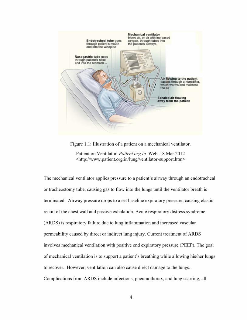
Mechanical ventilation can be used for breathing support in both acute and

chronic diseases (Figure 1.1).

4

The mechanical ventilator applies pressure to a patient’s airway through an endotracheal

or tracheostomy tube, causing gas to flow into the lungs until the ventilator breath is

terminated. Airway pressure drops to a set baseline expiratory pressure, causing elastic

recoil of the chest wall and passive exhalation. Acute respiratory distress syndrome

(ARDS) is respiratory failure due to lung inflammation and increased vascular

permeability caused by direct or indirect lung injury. Current treatment of ARDS

involves mechanical ventilation with positive end expiratory pressure (PEEP). The goal

of mechanical ventilation is to support a patient’s breathing while allowing his/her lungs

to recover. However, ventilation can also cause direct damage to the lungs.

Complications from ARDS include infections, pneumothorax, and lung scarring, all

Figure 1.1: Illustration of a patient on a mechanical ventilator.

Patient on Ventilator. Patient.org.in. Web. 18 Mar 2012 <http://www.patient.org.in/lung/ventilator-support.htm>

5

which can be caused by ventilation [4]. Deaths from ARDS usually results from multiple

system organ failure (MSOF). Research suggests mechanical ventilation triggers the

release of inflammatory mediators into the lungs and circulation, a mechanism termed

biotrauma, possibly causing MSOF [5]. Advances in ventilator strategies have reduced

ventilator-induced lung injury and mortality in ARDS patients [6]. Mechanical

ventilation could also be used for a short period to support respiratory function in chronic

lung disease patients. However, in 2011 the International Society for Heart and Lung

Transplantation reported ventilation prior to transplant as a significant risk factor for both

1-year and 5-year mortality in adult lung transplant recipients [2]. Thus, mechanical

ventilation is a contraindication for lung transplantation.

There are several alternatives to mechanical ventilation which provide either

partial or total respiratory support. Extracorporeal membrane oxygenation (ECMO, also

known as extracorporeal life support) is used to treat cardiac or respiratory failure

providing respiratory support (V-V ECMO) or respiratory and cardiac support (V-A

ECMO) for days or weeks. ECMO is prolonged extracorporeal (outside the body)

cardiopulmonary support through vascular cannulation. In V-V ECMO, blood is taken

from the venous system, routed through the circuit where it is oxygenated, and then

returned to the venous system (jugular vein in and out, or jugular vein to right femoral

vein). For V-A ECMO, blood is taken from the venous system and returned to the arterial

system (carotid artery and vein, femoral artery and vein, or aorta and right atrium). The

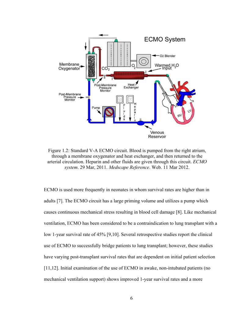
ECMO circuit is large, consisting of: a blood pump, a servoregulator, an oxygenator, a

heat exchanger, cannulas, tubing, and continuous heparin infusion (Figure 1.2).

6

ECMO is used more frequently in neonates in whom survival rates are higher than in

adults [7]. The ECMO circuit has a large priming volume and utilizes a pump which

causes continuous mechanical stress resulting in blood cell damage [8]. Like mechanical

ventilation, ECMO has been considered to be a contraindication to lung transplant with a

low 1-year survival rate of 45% [9,10]. Several retrospective studies report the clinical

use of ECMO to successfully bridge patients to lung transplant; however, these studies

have varying post-transplant survival rates that are dependent on initial patient selection

[11,12]. Initial examination of the use of ECMO in awake, non-intubated patients (no

mechanical ventilation support) shows improved 1-year survival rates and a more

Figure 1.2: Standard V-A ECMO circuit. Blood is pumped from the right atrium, through a membrane oxygenator and heat exchanger, and then returned to the

arterial circulation. Heparin and other fluids are given through this circuit. ECMO system. 29 Mar, 2011. Medscape Reference. Web. 11 Mar 2012.

7

promising bridging technique [13]. Advances in pump and oxygenator technology and

using ECMO as an alternative to mechanical ventilation have improved outcomes and

shown the possibility of using ECMO as a bridge to lung transplantation. However, it is

still an invasive, complex technique requiring a team of specialists and blood

transfusions. Because of its complexity and number of components, there are many

avenues for complications. Complication rates are reported by the ELSO registry, broken

down by type and mode of support [14]. Some of the most common are: oxygenator

failure (8-17%), blood clots in the system components (9-15%), cannula problems (5-

15%), and bleeding at the surgical site (6-33%) or cannula site (7-21%).

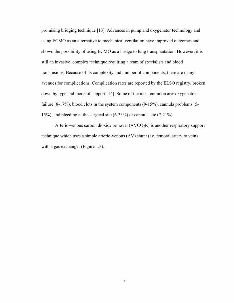
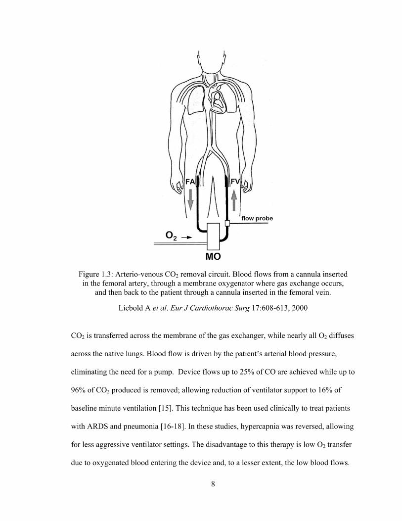
Arterio-venous carbon dioxide removal (AVCO2R) is another respiratory support

technique which uses a simple arterio-venous (AV) shunt (i.e. femoral artery to vein)

with a gas exchanger (Figure 1.3).

8

CO2 is transferred across the membrane of the gas exchanger, while nearly all O2 diffuses

across the native lungs. Blood flow is driven by the patient’s arterial blood pressure,

eliminating the need for a pump. Device flows up to 25% of CO are achieved while up to

96% of CO2 produced is removed; allowing reduction of ventilator support to 16% of

baseline minute ventilation [15]. This technique has been used clinically to treat patients

with ARDS and pneumonia [16-18]. In these studies, hypercapnia was reversed, allowing

for less aggressive ventilator settings. The disadvantage to this therapy is low O2 transfer

due to oxygenated blood entering the device and, to a lesser extent, the low blood flows.

Figure 1.3: Arterio-venous CO2 removal circuit. Blood flows from a cannula inserted in the femoral artery, through a membrane oxygenator where gas exchange occurs,

and then back to the patient through a cannula inserted in the femoral vein.

Liebold A et al. Eur J Cardiothorac Surg 17:608-613, 2000

9

Therefore, AVCO2R benefits patients with severe hypercapnia and ARDS, but not

patients with hypoxemia [8]. More recently, AVCO2R has been utilized for a bridge to

lung transplant [11, 19]; however, oxygenation was limited due to blood flow restrictions

and thus could only be used in patients with severe hypercapnia and only moderate

hypoxia. Also, only patients with adequate mean arterial pressure (>70 mmHg) and

sufficient cardiac output could undergo this procedure. Thus, this technique is not

adequate as a bridge to lung transplant.

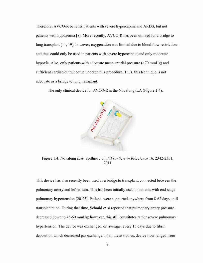
The only clinical device for AVCO2R is the Novalung iLA (Figure 1.4).

This device has also recently been used as a bridge to transplant, connected between the

pulmonary artery and left atrium. This has been initially used in patients with end-stage

pulmonary hypertension [20-23]. Patients were supported anywhere from 8-62 days until

transplantation. During that time, Schmid et al reported that pulmonary artery pressure

decreased down to 45-60 mmHg; however, this still constitutes rather severe pulmonary

hypertension. The device was exchanged, on average, every 15 days due to fibrin

deposition which decreased gas exchange. In all these studies, device flow ranged from

Figure 1.4: Novalung iLA. Spillner J et al. Frontiers in Bioscience 16: 2342-2351, 2011

10

1.8-3.0 L/min during support. This attachment mode allows the patient to be mobile;

however, with increasing physical activity CO increases. Schmid et al reported that as

their patient resumed physical activity, increased CO led to more flow through native

lung since flow to device couldn’t be increased. Thus, a larger fraction of unsaturated

blood arrived at the left atrium. The resistance of the Novalung is approximately 5-6

mmHg/(L/min) at blood flows of 2-2.5 L/min [17,18,24]. The Novalung was not intended

for PA-LA use when constructed. A device with lower resistance that allows for higher

flows would provide total respiratory support and allow patients to be ambulatory and

even exercise while awaiting lung transplant.

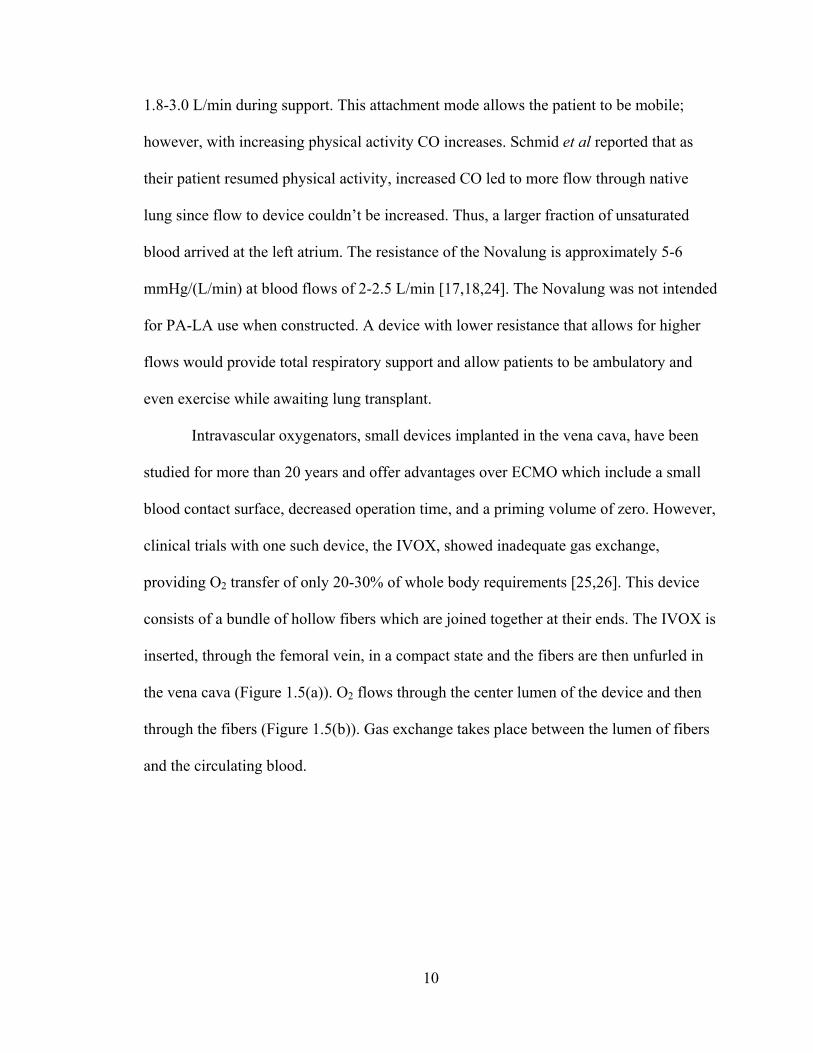
Intravascular oxygenators, small devices implanted in the vena cava, have been

studied for more than 20 years and offer advantages over ECMO which include a small

blood contact surface, decreased operation time, and a priming volume of zero. However,

clinical trials with one such device, the IVOX, showed inadequate gas exchange,

providing O2 transfer of only 20-30% of whole body requirements [25,26]. This device

consists of a bundle of hollow fibers which are joined together at their ends. The IVOX is

inserted, through the femoral vein, in a compact state and the fibers are then unfurled in

the vena cava (Figure 1.5(a)). O2 flows through the center lumen of the device and then

through the fibers (Figure 1.5(b)). Gas exchange takes place between the lumen of fibers

and the circulating blood.

11

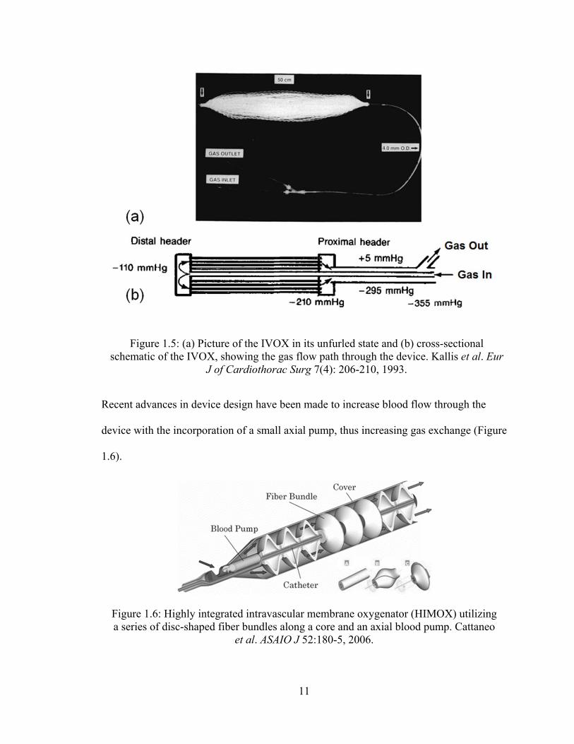
Recent advances in device design have been made to increase blood flow through the

device with the incorporation of a small axial pump, thus increasing gas exchange (Figure

1.6).

Figure 1.5: (a) Picture of the IVOX in its unfurled state and (b) cross-sectional schematic of the IVOX, showing the gas flow path through the device. Kallis et al. Eur

J of Cardiothorac Surg 7(4): 206-210, 1993.

Figure 1.6: Highly integrated intravascular membrane oxygenator (HIMOX) utilizing a series of disc-shaped fiber bundles along a core and an axial blood pump. Cattaneo

et al. ASAIO J 52:180-5, 2006.

12

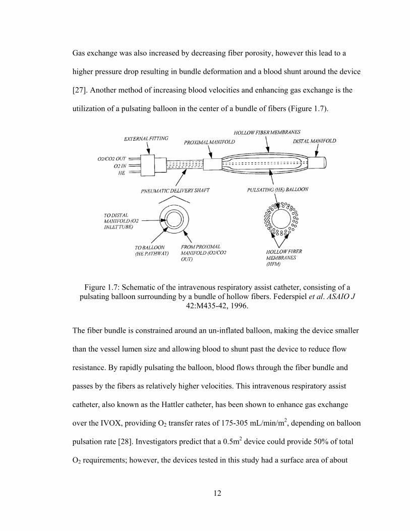
Gas exchange was also increased by decreasing fiber porosity, however this lead to a

higher pressure drop resulting in bundle deformation and a blood shunt around the device

[27]. Another method of increasing blood velocities and enhancing gas exchange is the

utilization of a pulsating balloon in the center of a bundle of fibers (Figure 1.7).

The fiber bundle is constrained around an un-inflated balloon, making the device smaller

than the vessel lumen size and allowing blood to shunt past the device to reduce flow

resistance. By rapidly pulsating the balloon, blood flows through the fiber bundle and

passes by the fibers as relatively higher velocities. This intravenous respiratory assist

catheter, also known as the Hattler catheter, has been shown to enhance gas exchange

over the IVOX, providing O2 transfer rates of 175-305 mL/min/m2, depending on balloon

pulsation rate [28]. Investigators predict that a 0.5m2 device could provide 50% of total

O2 requirements; however, the devices tested in this study had a surface area of about

Figure 1.7: Schematic of the intravenous respiratory assist catheter, consisting of a pulsating balloon surrounding by a bundle of hollow fibers. Federspiel et al. ASAIO J

42:M435-42, 1996.

13

0.23m2. Since intravascular oxygenators are small, bundle surface area must be

maximized to maximize gas transfer. However, this results in higher blood flow

resistance, reducing venous return to the heart. Thus, despite the above design

improvements, these devices cannot provide total respiratory support and are not a

sufficient bridge to lung transplant.

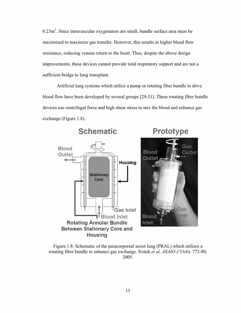
Artificial lung systems which utilize a pump or rotating fiber bundle to drive

blood flow have been developed by several groups [29-31]. These rotating fiber bundle

devices use centrifugal force and high shear stress to mix the blood and enhance gas

exchange (Figure 1.8).

Figure 1.8: Schematic of the paracorporeal assist lung (PRAL) which utilizes a rotating fiber bundle to enhance gas exchange. Svitek et al. ASAIO J 51(6): 773-80,

2005.

14

The disadvantage of these devices is the high shear rates which cause platelet activation

and hemolysis. Previous research demonstrated that platelet activation is a function of

shear stress magnitude and duration of application and that shear-induced platelet

activation occurs only above a threshold of 12-15 dyne/cm2 [32-34]. Svitek et al

estimated duration of support for their device to be 7-10 days. They reported high levels

of hemolysis at the higher rotating rates and calculated the maximum shear stress of their

device due to rotation to be 80 dynes/cm2. This is well above the threshold for shear-

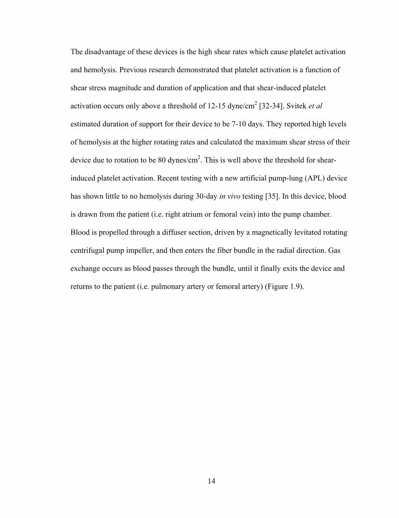
induced platelet activation. Recent testing with a new artificial pump-lung (APL) device

has shown little to no hemolysis during 30-day in vivo testing [35]. In this device, blood

is drawn from the patient (i.e. right atrium or femoral vein) into the pump chamber.

Blood is propelled through a diffuser section, driven by a magnetically levitated rotating

centrifugal pump impeller, and then enters the fiber bundle in the radial direction. Gas

exchange occurs as blood passes through the bundle, until it finally exits the device and

returns to the patient (i.e. pulmonary artery or femoral artery) (Figure 1.9).

15

This device has the advantage of being compact, with a small priming volume; however

it is only designed to provide blood flows of 3.5 L/min. Additional testing may be

required to examine device performance in ambulatory or exercising patients and patients

with pulmonary hypertension.

Thoracic Artificial Lung Development

The devices and techniques described above are either not suitable as a bridge to

lung transplant or too early in their development. Such a device must be durable, simple

to operate, provide total respiratory support, minimize blood damage and activation, and

have low resistance. This device must also allow patients to be awake and ambulatory

while awaiting lung transplant.

Figure 1.9: Cross-sectional view of the artificial pump lung (APL) showing the blood flow path. Wu et al. Ann Thorac Surg 93:274-81, 2012.

16

Thoracic artificial lungs (TAL) are being developed to meet these requirements.

TALs do not use a pump, but rather are attached to the pulmonary circulation with the

right ventricle (RV) driving blood flow. Elimination of the need for a blood pump greatly

reduces blood damage, coagulation, and inflammation. The patient’s own cardiac output

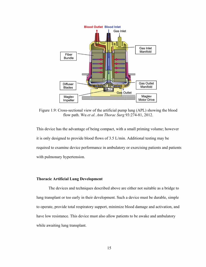
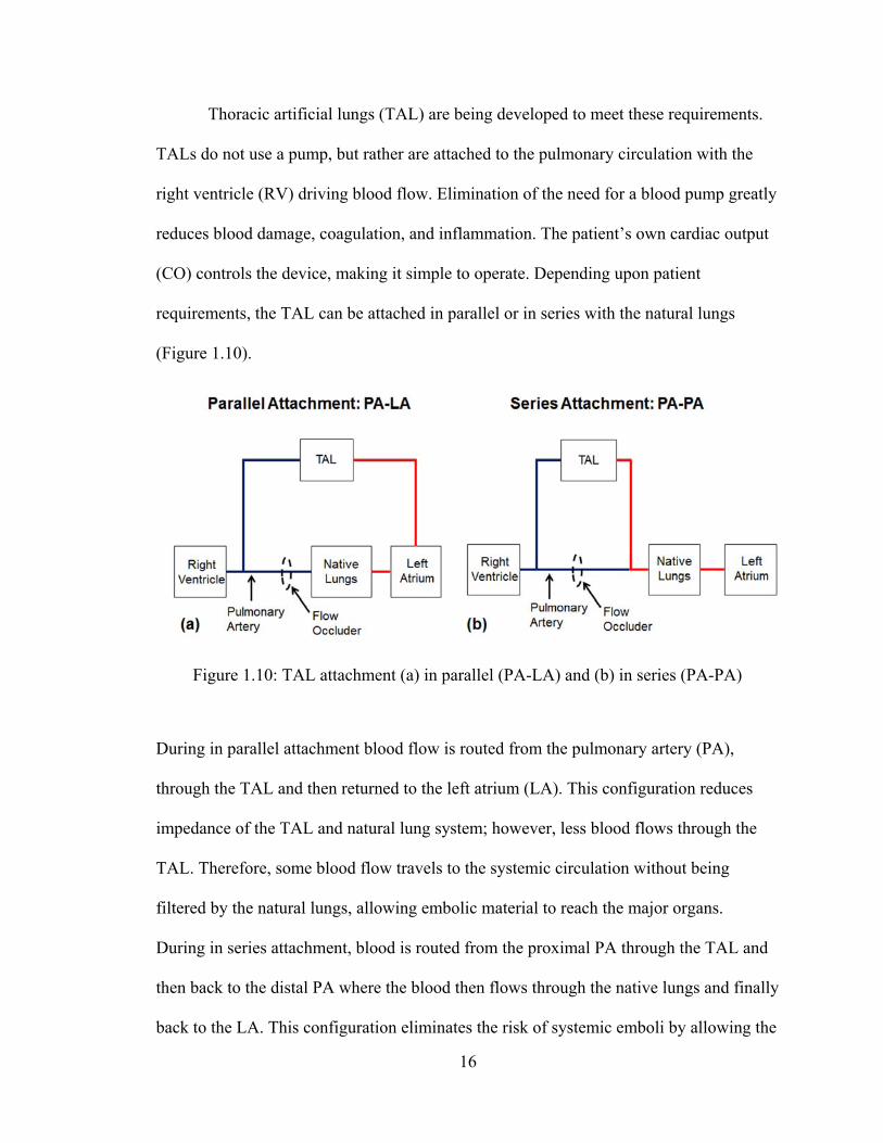
(CO) controls the device, making it simple to operate. Depending upon patient

requirements, the TAL can be attached in parallel or in series with the natural lungs

(Figure 1.10).

During in parallel attachment blood flow is routed from the pulmonary artery (PA),

through the TAL and then returned to the left atrium (LA). This configuration reduces

impedance of the TAL and natural lung system; however, less blood flows through the

TAL. Therefore, some blood flow travels to the systemic circulation without being

filtered by the natural lungs, allowing embolic material to reach the major organs.

During in series attachment, blood is routed from the proximal PA through the TAL and

then back to the distal PA where the blood then flows through the native lungs and finally

back to the LA. This configuration eliminates the risk of systemic emboli by allowing the

Figure 1.10: TAL attachment (a) in parallel (PA-LA) and (b) in series (PA-PA)

17

lung to perform its filtration and non-respiratory functions. In addition, the entire cardiac

output can flow through the TAL, allowing for complete gas exchange. Studies on TAL

attachment mode have shown parallel TAL attachment to decrease pulmonary system

impedance and increase CO, while in series attachment increases pulmonary system

impedance and decreases CO [36].

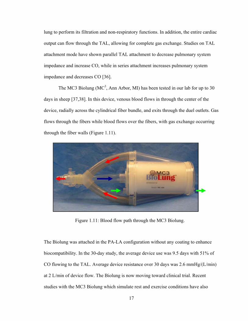
The MC3 Biolung (MC3, Ann Arbor, MI) has been tested in our lab for up to 30

days in sheep [37,38]. In this device, venous blood flows in through the center of the

device, radially across the cylindrical fiber bundle, and exits through the duel outlets. Gas

flows through the fibers while blood flows over the fibers, with gas exchange occurring

through the fiber walls (Figure 1.11).

The Biolung was attached in the PA-LA configuration without any coating to enhance

biocompatibility. In the 30-day study, the average device use was 9.5 days with 51% of

CO flowing to the TAL. Average device resistance over 30 days was 2.6 mmHg/(L/min)

at 2 L/min of device flow. The Biolung is now moving toward clinical trial. Recent

studies with the MC3 Biolung which simulate rest and exercise conditions have also

Figure 1.11: Blood flow path through the MC3 Biolung.

18

shown advantages in placing the device in parallel [39]. CO was maintained with high

flows to the TAL in rest and ambulatory conditions. At exercise conditions, CO

decreased with increasing flow to the TAL. Further decreases in device impedance are

necessary for increased exercise tolerance.

Despite promising Biolung results, in series attachment would still be desired if it

did not induce RV dysfunction. However, current TALs possess blood flow impedances

greater than the natural lungs, resulting in low CO when implanted in series with the

natural lung [40]. Increased pulmonary system impedance in the in series configuration is

caused by the additive impedance of the TAL and natural lung. This induces low CO via

increased RV oxygen demand, decreased RV oxygen supply, decreased contractile

function, and pulmonic valve dysfunction [41-43]. Patients with respiratory failure,

specifically those suffering from PH, may not be able to tolerate any additional

impedance from the TAL. In PH the PA pressure is high, causing increased work for the

right heart and often results in RV failure. Therefore, in series attachment of the TAL will

further increase pulmonary system impedance and the right heart workload, possibly

hastening RV failure.

Impedance is the opposition to pulsatile blood flow and is determined from a

relationship between the time-varying components of pressure and flow. Fourier

transforms are used to convert pressure, P(t), and flow, Q(t), waveforms in the time

domain into a series of sinusoids at their respective harmonics frequencies:

)sin()(1

0 nn

N

nn tPPtP

)sin()(1

0 nn

N

nn tQQtQ

19

where P0 and Q0 are the average pressure and flow magnitudes. The sinusoid at each

harmonic, n, has its own magnitude (Pn or Qn), frequency (ω), and phase shift (φ).

Harmonic frequencies are equal to integer multiples of the heart rate. Impedance is

defined as the ratio of the pressure magnitude to flow magnitude at each harmonic:

n

nn Q

PZ

The zeroth and first harmonic impedance moduli (Z0 and Z1), are most physically

relevant as the opposition to steady flow and flow at a frequency equal to the heart rate,

respectively. Since CO is affected mostly by Z0 and Z1, e these are our focus. Impedance

is a function of TAL resistance, compliance, and inertance, with impedance increasing

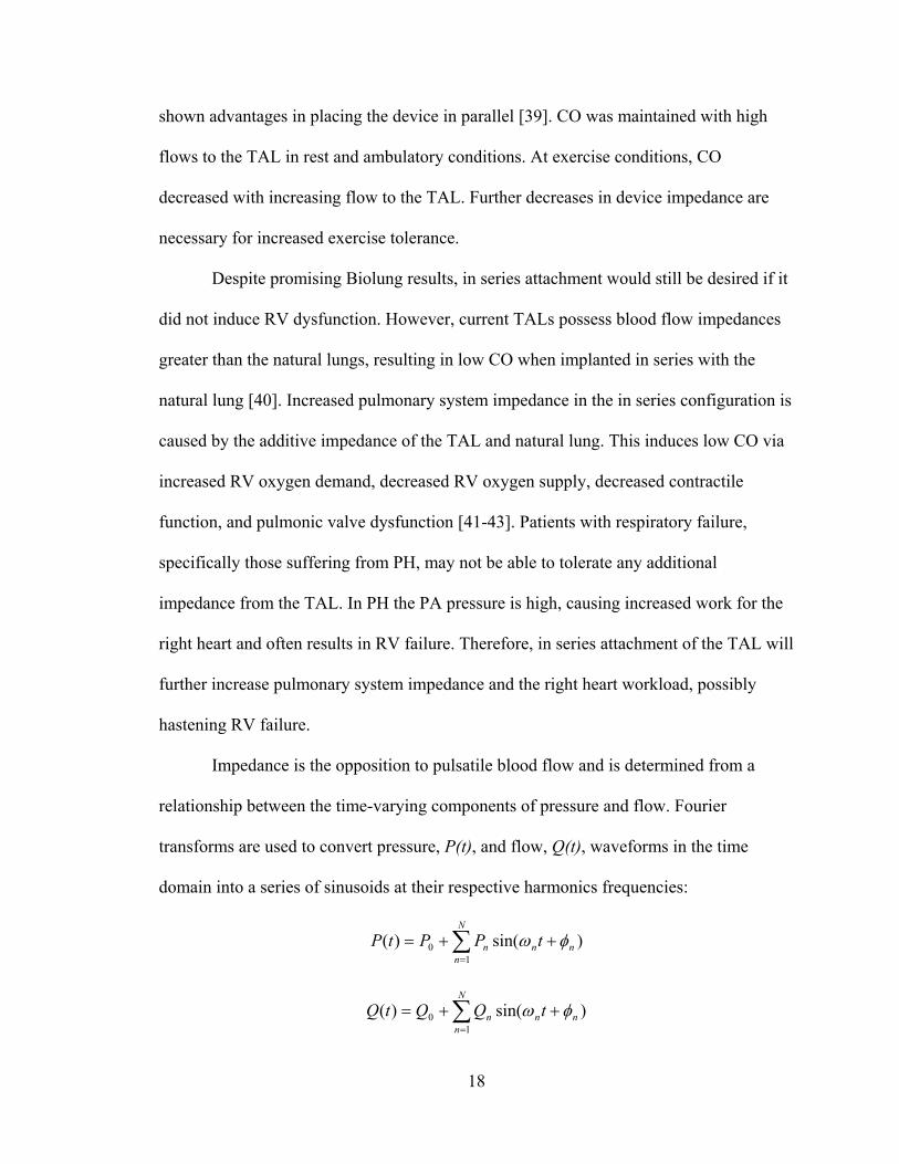
with increasing resistance and inertance and decreasing with increasing compliance. An

inlet compliance chamber (Figure 1.12) has been shown to reduce Z1 by nearly 80% and

to a lesser extent, Z0 in both in vitro and in vivo studies [40,44,45].

Figure 1.12: Biolung with a polyurethane compliance chamber attached to its inlet. McGillicuddy et al. ASAIO J 51:789-794, 2005.

20

McGillicuddy et al minimized Z0 and Z1 in vitro at compliances greater than 1 and 5

ml/mmHg, respectively. By reducing device impedance, the work of the RV is also

reduced by dampening the pulsatile flow and creating a more steady flow throughout the

cardiac cycle. Despite reducing device impedance, overall system impedance (Z0=5.75

mmHg/(L/min) and Z1=2.41 mmHg/(L/min)) was still greater than that of the natural

lungs (baseline Z0=2.87 mmHg/(L/min) and Z1=0.96 mmHg/(L/min)) during in series

attachment, causing a decrease in CO. Sato et al suggest that most of the RV dysfunction

is due to an increase in the zeroth harmonic impedance, Z0, due to its effects on average

system pressures, and a smaller decrease in CO is caused by the first harmonic

impedance modulus, Z1, due to its effect on systolic pressures. Kuo et al confirmed that

Z0 is the key determinant of RV output in their study examining the effect of pulmonary

system impedance on CO [46]. For every 1 mmHg/(L/min) increase in Z0 there is an

approximate 3.65% decrease in CO. Likewise, for every 1 mmHg/(L/min) increase in Z1

there is a 0.08Z0% decrease in CO. Akay et al performed a similar study, examining the

relationship between pulmonary system impedance on CO in sheep with pulmonary

hypertension [47]. Results again indicated that Z0 had a significant effect on percent

change in CO, %ΔCO, and found that: %ΔCO = -7.45*ΔZ0. Therefore, the foremost goal

of TAL design should be to reduce Z0, with a secondary requirement to limit increases in

Z1. Sato et al concluded that the resistance of the compliance chamber, device or

anastomoses must be reduced to improve CO [40]. The compliance chamber design has a

limited volume and a large expansion and contraction which significantly adds to the

system resistance, and thus a compliant device is proposed.

21

Compliant TAL

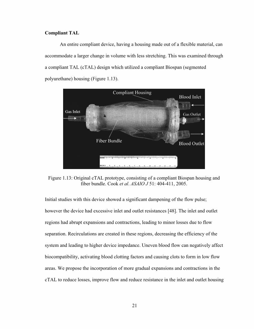
An entire compliant device, having a housing made out of a flexible material, can

accommodate a larger change in volume with less stretching. This was examined through

a compliant TAL (cTAL) design which utilized a compliant Biospan (segmented

polyurethane) housing (Figure 1.13).

Initial studies with this device showed a significant dampening of the flow pulse;

however the device had excessive inlet and outlet resistances [48]. The inlet and outlet

regions had abrupt expansions and contractions, leading to minor losses due to flow

separation. Recirculations are created in these regions, decreasing the efficiency of the

system and leading to higher device impedance. Uneven blood flow can negatively affect

biocompatibility, activating blood clotting factors and causing clots to form in low flow

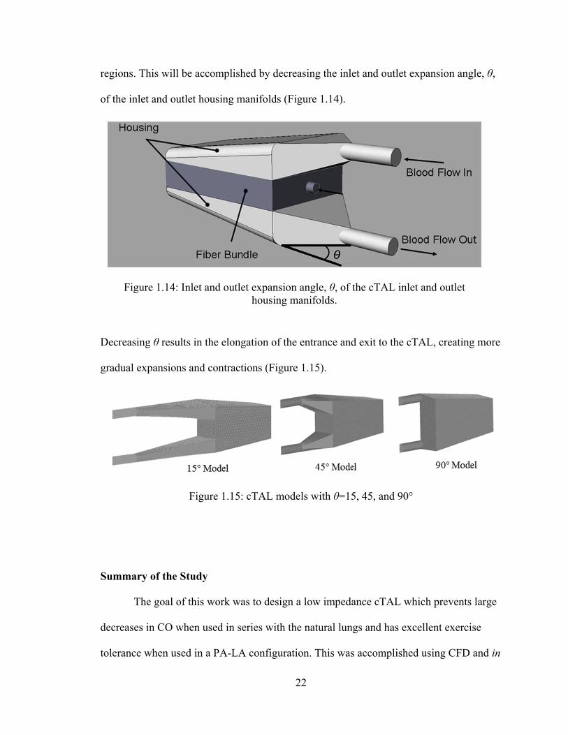
areas. We propose the incorporation of more gradual expansions and contractions in the

cTAL to reduce losses, improve flow and reduce resistance in the inlet and outlet housing

Figure 1.13: Original cTAL prototype, consisting of a compliant Biospan housing and fiber bundle. Cook et al. ASAIO J 51: 404-411, 2005.

22

regions. This will be accomplished by decreasing the inlet and outlet expansion angle, θ,

of the inlet and outlet housing manifolds (Figure 1.14).

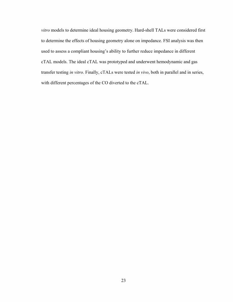
Decreasing θ results in the elongation of the entrance and exit to the cTAL, creating more

gradual expansions and contractions (Figure 1.15).

Summary of the Study

The goal of this work was to design a low impedance cTAL which prevents large

decreases in CO when used in series with the natural lungs and has excellent exercise

tolerance when used in a PA-LA configuration. This was accomplished using CFD and in

Figure 1.14: Inlet and outlet expansion angle, θ, of the cTAL inlet and outlet housing manifolds.

Figure 1.15: cTAL models with θ=15, 45, and 90°

23

vitro models to determine ideal housing geometry. Hard-shell TALs were considered first

to determine the effects of housing geometry alone on impedance. FSI analysis was then

used to assess a compliant housing’s ability to further reduce impedance in different

cTAL models. The ideal cTAL was prototyped and underwent hemodynamic and gas

transfer testing in vitro. Finally, cTALs were tested in vivo, both in parallel and in series,

with different percentages of the CO diverted to the cTAL.

24

References

1. American Lung Association Lung Disease Data, 2008. www.lungusa.org

2. Christie JD, Edwards LB, Kucheryavaya AY, et al. The Registry of the

International Society for Heart and Lung Transplantation: Twenty-eighth Adult

Lung and Heart-Lung Transplantation Report--2011. Journal of Heart & Lung

Transplantation 30: 1104-22, 2011.

3. 2009 OPTN/SRTR Annual Report. Available at: http://optn.transplant.hrsa.gov.

Accessed February 6, 2012.

4. National Institutes of Health. National Heart, Lung and Blood Institute. Diseases

and Conditions Index. Acute Respiratory Distress Syndrome (ARDS): Treatment.

January 2012. Available at

http://www.nhlbi.nih.gov/health/dci/Diseases/Ards/Ards_Treatments.html.

Accessed on February 7, 2012.

5. Plötz FB, Slutsky AS, van Vught AJ, Heijnen CJ: Ventilator-induced lung injury

and multiple system organ failure: a critical review of facts and hypotheses.

Intensive Care Med 30: 1865-1872, 2004.

6. Slutsky AS, Ranieri VM: Mechanical ventilation: lessons from the ARDSNet

trial. Respir Res 1: 73-77, 2000.

7. Bartlett RH, Roloff DW, Custer JR, Younger JG, Hirschl RB. Extracorporeal life

support - The University of Michigan experience. JAMA 283: 904-908, 2000.

8. Kopp R, Dembinski R, Kuhlen R. Role of extracorporeal lung assist in the

treatment of acute respiratory failure. Minerva Anestesiol 72: 587-95, 2006.

25

9. Mason DP, Thuita L, Nowicki ER, et al. Should lung transplantation be

performed for patients on mechanical respiratory support? The US experience. J

Cardiovasc Surg 139:765-73, 2010.

10. Russo MJ, Davies RR, Hong KN, et al. Who is the high-risk recipient? Predicting

mortality after lung transplantation using pretransplant risk factors. J Thorac

Cardiovasc Surg 138: 1234-1238, 2009.

11. Haneya A, Philipp A, Mueller T, et al. Extracorporeal Circulatory Systems as a

Bridge to Lung Transplantation at Remote Transplant Centers. Ann Thorac Surg

91:250-6, 2011.

12. Bermudez CA, Rocha RV, Zaldonis D, et al. Extracorporeal Membrane

Oxygenation as a Bridge to Lung Transplant: Midterm Outcomes. Ann Thorac

Surg 92:1226-32, 2011.

13. Fuehner T, Kuehn C, Hadem J, et al. Extracorporeal Membrane Oxygenation in

Awake Patients as Bridge to Lung Transplantation. Am J Respir Crit Care Med

[Epub ahead of print], 2012.

14. ECLS Registry Report. International Summary; January, 2012. Extracorporeal

Life Support Organization, Ann Arbor, MI.

15. Zwischenberger JB, Alpard SK. Artificial lungs: a new inspiration. Perfusion 17:

253-268, 2002.

16. Bein T, Weber F, Philipp A, et al. A new pumpless extracorporeal interventional

lung assist in critical hypoxemia/hypercapnia. Crit Care Med 34:1372-1377,

2006.

26

17. Müller T, Lubnow M, Philipp A, Bein T, Jeron A, Luchner A, Rupprecht L, Reng

M, Langgartner J, Wrede CE, Zimmermann M, Birnbaum D, Schmid C, Riegger

GA, Pfeifer M. Extracorporeal pumpless interventional lung assist in clinical

practice: determinants of efficacy. Eur Respir J 33:551-8, 2009.

18. Flörchinger B, Philipp A, Klose A, Hilker M, Kobuch R, Rupprecht L, Keyser A,

Pühler T, Hirt S, Wiebe K, Müller T, Langgartner J, Lehle K, Schmid C.

Pumpless extracorporeal lung assist: a 10-year institutional experience. Ann

Thorac Surg 86:410-7, 2008.

19. Fischer S, Simon AR, Welte T, et al. Bridge to lung transplantation with the novel

pumpless interventional lung assist device NovaLung. J Cardiovasc Surg

131:719-23, 2006.

20. Schmid C, Philipp A, Hilker M, et al. Bridge to Lung Transplantation Through a

Pulmonary Artery to Left Atrial Oxygenator Circuit. Ann Thorac Surg 85:1202-5,

2008.

21. Camboni D, Philipp A, Arlt M, et al. First Experience With a Paracorporeal

Artificial Lung in Humans. ASAIO J 55:304-307, 2009.

22. Strueber M, Hoeper MM, Fischer S, et al. Bridge to Thoracic Organ

Transplantation in Patients with Pulmonary Arterial Hypertension Using a

Pumpless Lung Assist Device. American Journal of Transplantation 9:853-857,

2009.

23. Gazit AZ, Sweet SC, Grady RM, Huddleston CB. First experience with a

paracorporeal artificial lung in a small child with pulmonary hypertension. J

Thorac Cardiovasc Surg 141: e45-50, 2011

27

24. Wiebe K, Poeling J, Arlt M, Philipp A, Camboni D, Hofmann S, Schmid C.

Thoracic surgical procedures supported by a pumpless interventional lung assist.

Ann Thorac Surg 89:1782-7, 2010.

25. Kallis P, al-Saady NM, Bennett ED, Treasure T. Early results of intravascular

oxygenation. European Journal of Cardiothoracic Surgery 7(4): 206-210, 1993.

26. Gentiello LM, Jurkovich GJ, Gubler D, Anardi DM, Heiskell R. The Intravascular

Oxygenator (IVOX): Preliminary Results of a New Means of Performing

Extrapulmonary Gas Exchange. Journal of Trauma 35: 399-404, 1993.

27. Cattaneo GFM, Reul H, Schmitz-Rode R, Steinseifer U. Intravascular Blood

Oxygenation Using Hollow Fiber in a Disk-Shaped Configuration: Experimental

Evaluation of the Relationship Between Porosity and Performance. ASAIO J 52:

180-185, 2006.

28. Federspiel WJ, Golob JF, Merrill TL, et al. Ex vivo testing of the intravenous

membrane oxygenator. ASAIO J 46:261-7, 2000.

29. Svitek RG, Frankowski BJ, Federspiel WJ. Evaluation of a Pumping Assist Lung

That Uses a Rotating Fiber Bundle. ASAIO J 51(6): 773-80, 2005.

30. Wu ZJ, Gartner M, Litwak KN, Griffith BP. Progress toward an ambulatory

pump-lung. J Thorac Cardiovasc Surg 130: 973-78, 2005.

31. Makarewicz AJ, Mockros LF, Mavroudis C. New Design for a Pumping Artificial

Lung. ASAIO J 42: M615-9, 1996.

32. Cook KE, Maxhimer J, Leonard DJ, Mavroudis C, Backer CL, Mockros LF:

Platelet and Leukocyte Activation and Design Consequences for Thoracic

Artificial Lungs. ASAIO Journal 48(6): 620-30, 2002.

28

33. Cook KE, Mockros LF. Biocompatibility of artificial lungs. In The Artificial

Lung. Vaslef SN, Anderson RW, eds. Landes Bioscience. Austin, TX. 2002.

34. Chow, T.W., Hellums, J.D., Moake, J.L., and Kroll, M.H: Shear stress-induced

von Willebrand factor binding to platelet glycoprotein Ib initiates calcium influx

associated with aggregation. Blood 80 (1): 113-120, 1992.

35. Wu ZJ, Zhang T, Bianchi G, et al. Thirty-Day In-Vivo Performance of a

Wearable Artificial Pump-Lung for Ambulatory Respiratory Support. Ann Thorac

Surg 93:274-81, 2011.

36. Perlman CE, Cook KE, Seipelt R, Mavroudis C, Backer CL, Mockros LF. In vivo

hemodynamic responses to artificial lung attachment. ASAIO J 51: 412-425, 2005.

37. Sato H, Griffith GW, Hall CM, et al: Seven-Day Artificial Lung Testing in an In-

Parallel Configuration. Ann Thorac Surg 84: 988-94, 2007.

38. Sato H, Hall CM, Lafayette NG, et al: Thirty-Day In-Parallel Artificial Lung

Testing in Sheep. Ann Thorac Surg 84: 1136-43, 2007.

39. Akay B, Reoma JL, Camboni D, et al. In-parallel artificial lung attachment at high

flows in normal and pulmonary hypertension models. Ann Thorac Surg 90: 259-

65, 2010.

40. Sato H, McGillicuddy JH, Griffith GW, et al: Effect of Artificial Lung

Compliance on In Vivo Pulmonary System Hemodynamics. ASAIO J 52: 248-

256, 2006.

41. Kuo AS, Perlman CE, Mockros LF, Cook KE: Pulmonic Valve Function During

Thoracic Artifical Lung Attachment. ASAIO J 54: 197-202, 2008.

29

42. Brooks H, Kirk ES, Vokonas PS, Urschel CW, Sonnenblick EH: Performance of

the Right Ventricle under Stress: Relation to Right Coronary Flow. J Clin Invest

50: 2176-2183, 1971.

43. Vlahakes GJ, Turley K, Hoffman JI: The pathophysiology of failure in acute right

ventricular hypertension: hemodynamic and biochemical correlations. Circulation

63: 87-95, 1981.

44. McGillicuddy JW, Chambers SD, Galligan DT, Hirschl RB, Bartlett RH, Cook

KE. In vitro, fluid mechanical effects of thoracic artificial lung compliance.

ASAIO J 51:789-794, 2005.

45. Haft JW, Bull JL, Rose R, Katsra J, Grotberg JB, Bartlett RH, Hirschl RB. Design

of an Artificial Lung Compliance Chamber for Pulmonary Replacement. ASAIO J

49: 35-40, 2003.

46. Kuo AS, Sato H, Reoma JL, Cook KE. The relationship between pulmonary

system impedance and right ventricular function in normal sheep. Cardiovascular

Engineering 9: 153-160, 2009.

47. Akay B, Foucher JA, Camboni D, Koch KL, Kawatra A, Cook KE.

Hemodynamic design requirements for in series thoracic artificial lung attachment

in a model of pulmonary hypertension. ASAIO Journal, Epub ahead of print.

48. Cook KE, Perlman CE, Seipelt R, et al: Hemodynamic and Gas Transfer

Properties of a Compliant Thoracic Artificial Lung. ASAIO J 51: 404-411, 2005.

30

Chapter 2

Thoracic Artificial Lung Housing Design

Introduction

Current TALs and cTALs possess blood flow impedances greater than the natural

lungs, resulting in abnormal pulmonary hemodynamics when implanted in series with the

natural lung or in parallel with high flows to the TAL [1,2]. Previous studies have shown

the majority of cTAL impedance was due to excessive inlet/outlet impedances [3]. It was

theorized that the abrupt expansions and contractions at the inlet and outlet regions cause

flow recirculation that, in turn, leads to higher device impedance. If this is the case, more

gradual expansions and contractions could improve flow patterns and reduce device

impedance. Device design also influences flow uniformity within the cTAL. It is essential

to have even flow throughout the fiber bundle and housing in order to have efficient gas

transfer and eliminate any low flow areas where blood clots can form. Thus, device

design is essential to optimize both the impedance and biocompatibility of the cTAL.

The effect of housing geometry on cTAL impedance will be explored in Chapter

3 using fluid-structure interaction (FSI) modeling. However, the influence of housing

geometry alone will first be considered in simplified, rigid-housing TAL designs. In this

chapter, the inlet and outlet expansion angle, θ, of the TAL was adjusted, and flow

patterns and impedance were determined at a variety of blood flow rates and heart rates.

31

First, computational fluid dynamics (CFD) was used to examine the effects of different

housing designs on device flow patterns and impedance. Flow patterns are important in

predicting gas transfer performance and biocompatibility and cannot be easily visualized

in vitro. Second, physical models were created and tested in vitro to verify computer

results.

Methods

Computational Fluid Dynamics Studies

The effects of θ on TAL blood flow patterns and impedance were evaluated using

designs with θ= 15°, 45° and 90° (Figure 2.1).

SolidWorks (Dassault Systèmes SolidWorks Corp, Concord, MA) computer-aided design

(CAD) software was used to create each housing model, which was then imported into

the ADINA (ADINA R&D Inc., Watertown, MA) computational fluid dynamics (CFD)

software program (Figure 2.2).

Figure 2.1: TAL model showing blood flow path and inlet and outlet expansion angle, θ

32

In these models, blood flows through the inlet, expands into the inlet manifold, flows

through the fiber bundle at the center of the device, then travels through the outlet

manifold and exits through the device outlet. The inlet/outlet diameter, height and width

of each TAL model are 0.016 m, 0.103 m and 0.102 m, respectively. The fiber bundle

length, path length (the distance blood must flow through the bundle), and frontal area

(the cross-sectional area perpendicular to blood flow through the bundle) are 0.140 m,

0.038 m, and 0.016 m2, respectively, for each model. The 15°, 45°, and 90° models have

a total length of 0.350 m, 0.229 m, and 0.191 m. Since the inlet/outlet tube diameter and

the housing body geometry is fixed, the length of the expansion/contraction section

increases as θ decreases (see Figure 2.1).

CFD: Problem Formulation

Program assumptions included a transient solution with incompressible flow.

Turbulent flow was assumed to occur in the inlet and outlet sections. The average

Reynolds numbers in the inlet and outlet sections at flow rates of 2, 4, and 6 L/min are

920, 1800, and 2760, respectively. Peak Reynolds numbers at these same flows are 3000,

6100, and 9200, respectively. The material properties of the rigid housing and fiber

Figure 2.2: TAL housing models used for CFD study with θ = 15°, 45° and 90°

33

bundle, along with the fluid characteristics of blood were defined in the program. Blood

viscosity and density were set to 0.003 Pa s (3.0 cP) and 1040 kg/m3. The fiber bundle

region was modeled as porous media with fluid density, porosity, permeability, and fluid

viscosity defined as 1040 kg/m3, 0.75, 2.81x10-9 m2, and 0.003 Pa s (3.0 cP),

respectively. Permeability, k, was calculated from preliminary cTAL data [3] using

Darcy’s Law:

PA

LQk

(1)

where Q is blood flow rate, μ is viscosity, L is the fiber bundle path length, A is the fiber

bundle frontal area, and ΔP is the pressure drop across the fiber bundle. The hollow fiber

bundle was modeled using a porous media theory to determine flow characteristics within

the bundle [4-7].

The fluid motion outside the fiber bundle is governed by the Navier-Stokes

equations with constant density and viscosity, together with the continuity equation as

follows:

VVVV 2

fff Pt

(2)

0 V (3)

where f is the blood density, f is the blood viscosity, P is the pressure and V is the

velocity vector.

CFD: Boundary Conditions

A symmetry condition was utilized in ADINA, allowing the model to be cut in

half, thus reducing computational time. This was done by applying a zero velocity fixity

34

perpendicular to the symmetry face. A no-slip wall boundary condition was also applied

to the inlet and outlet housings, while a slip wall boundary condition was applied to the

bundle walls. The momentum equation used in the porous media model does not contain

any second order derivatives, thus viscous effects are negligible and a slip wall condition

is used. The initial pressure condition was set to 10 mmHg. A time dependent velocity

was applied to the inlet face and a constant pressure of 10 mmHg was applied to the

outlet face to simulate left atrial pressure.

Pulsatile blood flow through the device was simulated in ADINA at average flow

rates (Q) of 2, 4, and 6 L/min and heart rates (HR) of 80 and 100 beats/min (Figure 2.3).

Figure 2.3: TAL inlet flow waveform for CFD and in vitro studies at 4 L/min, 100 beats/min, and pulsatilities of 2 and 3.75.

35

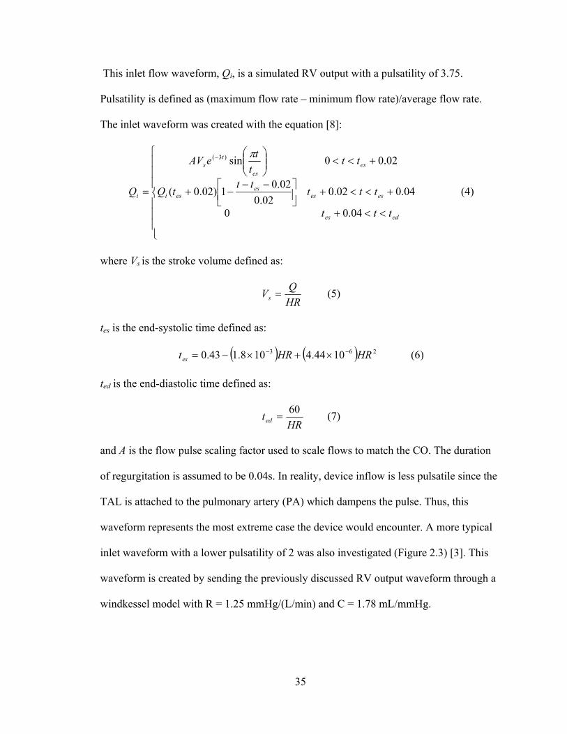
This inlet flow waveform, Qi, is a simulated RV output with a pulsatility of 3.75.

Pulsatility is defined as (maximum flow rate – minimum flow rate)/average flow rate.

The inlet waveform was created with the equation [8]:

edes

eseses

esi

eses

ts

i

ttt

ttttt

tQ

ttt

teAV

Q

04.00

04.002.002.0

02.01)02.0(

02.00sin)3(

(4)

where Vs is the stroke volume defined as:

HR

QVs (5)

tes is the end-systolic time defined as:

263 1044.4108.143.0 HRHRtes (6)

ted is the end-diastolic time defined as:

HRted

60 (7)

and A is the flow pulse scaling factor used to scale flows to match the CO. The duration

of regurgitation is assumed to be 0.04s. In reality, device inflow is less pulsatile since the

TAL is attached to the pulmonary artery (PA) which dampens the pulse. Thus, this

waveform represents the most extreme case the device would encounter. A more typical

inlet waveform with a lower pulsatility of 2 was also investigated (Figure 2.3) [3]. This

waveform is created by sending the previously discussed RV output waveform through a

windkessel model with R = 1.25 mmHg/(L/min) and C = 1.78 mL/mmHg.

36

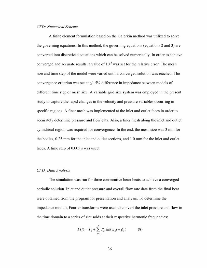
CFD: Numerical Scheme

A finite element formulation based on the Galerkin method was utilized to solve

the governing equations. In this method, the governing equations (equations 2 and 3) are

converted into discretized equations which can be solved numerically. In order to achieve

converged and accurate results, a value of 10-5 was set for the relative error. The mesh

size and time step of the model were varied until a converged solution was reached. The

convergence criterion was set at ≤1.5% difference in impedance between models of

different time step or mesh size. A variable grid size system was employed in the present

study to capture the rapid changes in the velocity and pressure variables occurring in

specific regions. A finer mesh was implemented at the inlet and outlet faces in order to

accurately determine pressure and flow data. Also, a finer mesh along the inlet and outlet

cylindrical region was required for convergence. In the end, the mesh size was 3 mm for

the bodies, 0.25 mm for the inlet and outlet sections, and 1.0 mm for the inlet and outlet

faces. A time step of 0.005 s was used.

CFD: Data Analysis

The simulation was run for three consecutive heart beats to achieve a converged

periodic solution. Inlet and outlet pressure and overall flow rate data from the final beat

were obtained from the program for presentation and analysis. To determine the

impedance moduli, Fourier transforms were used to convert the inlet pressure and flow in

the time domain to a series of sinusoids at their respective harmonic frequencies:

)sin()(1

0 nn

N

nn tPPtP

(8)

37

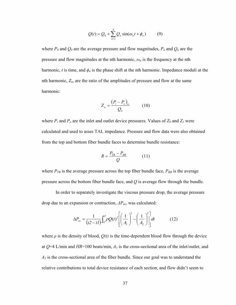
)sin()(1

0 nn

N

nn tQQtQ

(9)

where P0 and Q0 are the average pressure and flow magnitudes, Pn and Qn are the

pressure and flow magnitudes at the nth harmonic, ωn is the frequency at the nth

harmonic, t is time, and ϕn is the phase shift at the nth harmonic. Impedance moduli at the

nth harmonic, Zn, are the ratio of the amplitudes of pressure and flow at the same

harmonic:

n

noin Q

PPZ

(10)

where Pi and Po are the inlet and outlet device pressures. Values of Z0 and Z1 were

calculated and used to asses TAL impedance. Pressure and flow data were also obtained

from the top and bottom fiber bundle faces to determine bundle resistance:

Q

PPR BBTB (11)

where PTB is the average pressure across the top fiber bundle face, PBB is the average

pressure across the bottom fiber bundle face, and Q is average flow through the bundle.

In order to separately investigate the viscous pressure drop, the average pressure

drop due to an expansion or contraction, ΔPec, was calculated:

t2

t1ec dtAA

tQt1t2

P2

2

2

1

2 11)(

1 (12)

where ρ is the density of blood, Q(t) is the time-dependent blood flow through the device

at Q=4 L/min and HR=100 beats/min, A1 is the cross-sectional area of the inlet/outlet, and

A2 is the cross-sectional area of the fiber bundle. Since our goal was to understand the

relative contributions to total device resistance of each section, and flow didn’t seem to

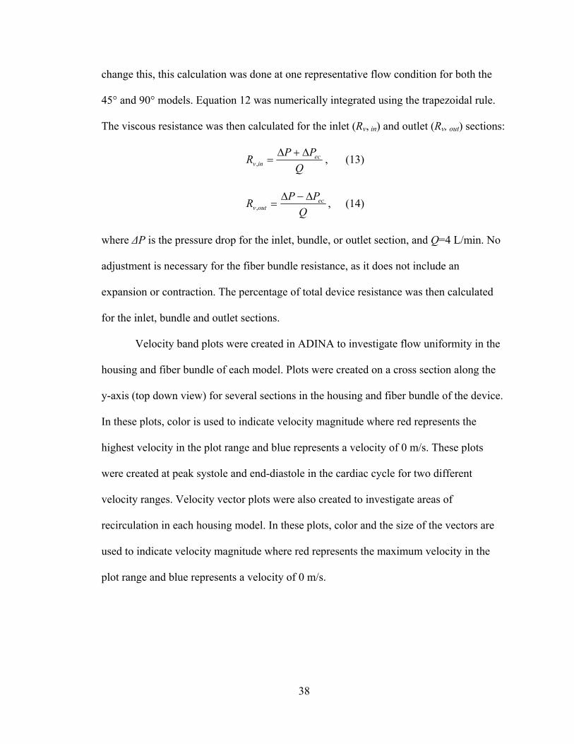
38

change this, this calculation was done at one representative flow condition for both the

45° and 90° models. Equation 12 was numerically integrated using the trapezoidal rule.

The viscous resistance was then calculated for the inlet (Rv, in) and outlet (Rv, out) sections:

Q

PPR ec

inv

, , (13)

Q

PPR ec

outv

, , (14)

where ΔP is the pressure drop for the inlet, bundle, or outlet section, and Q=4 L/min. No

adjustment is necessary for the fiber bundle resistance, as it does not include an

expansion or contraction. The percentage of total device resistance was then calculated

for the inlet, bundle and outlet sections.

Velocity band plots were created in ADINA to investigate flow uniformity in the

housing and fiber bundle of each model. Plots were created on a cross section along the

y-axis (top down view) for several sections in the housing and fiber bundle of the device.

In these plots, color is used to indicate velocity magnitude where red represents the

highest velocity in the plot range and blue represents a velocity of 0 m/s. These plots

were created at peak systole and end-diastole in the cardiac cycle for two different

velocity ranges. Velocity vector plots were also created to investigate areas of

recirculation in each housing model. In these plots, color and the size of the vectors are

used to indicate velocity magnitude where red represents the maximum velocity in the

plot range and blue represents a velocity of 0 m/s.

39

In Vitro Testing

Experimental tests were run on two TAL rigid housing models to validate the

computer results. The models tested had θ = 45° and 90°. To create the fiber bundle,

woven mats of polypropylene fibers with a fiber diameter of 200 μm were wound into

compact bundles with porosity, path length, and frontal area of 0.75, 0.038 m, and 0.016

m2, respectively. The bundle was potted with WC7-53 (BJB Enterprises Inc., Tustin,

CA), a two part polyurethane, into an acrylic box. Three sets of housings for each θ were

machined from PVC blocks and then clamped above and below a fiber bundle. The

blocks were carved out in the center, so that they are the negative of the housing shown in

Figure 2.1. In vitro testing was conducted with a circuit consisting of a pulsatile pump

(Harvard Apparatus, Holliston, MA), TAL model, and reservoir. The entire circuit was

primed with a 3.0 cP glycerol solution (Figure 2.4).

Pressure transducers (see Figure 2.4) were connected to six luers on the model in

order to monitor device pressure at the inlet (P1), outlet (P2), top of the bundle (P3 and

P5), and bottom of the bundle (P4 and P6). A blood flow probe was placed before the

Figure 2.4: In vitro test circuit consisting of a pulsatile pump, TAL model, and reservoir filled with 3.0 cP glycerol solution. Six pressure lines were connected to the model at the inlet (P1), outlet (P2), top of the bundle (P3 and P5), and bottom of the

bundle (P4 and P6).

40

device inlet to monitor flow rate. Using the pulsatile pump, testing was conducted for

HR= 80 and 100 beats/min and Q= 2, 4, and 6 L/min. Average pulsatilities for these

flows were 3.33. A representative inlet flow rate waveform at a HR=100 beats/min, Q=4

L/min, and pulsatility = 3.33 is shown in Figure 2.3. In addition, the 45° model was

tested at a pulsatility of 1.7 with HR=100 beats/min and Q=4 L/min to examine the

effects of pulsatility on device impedance. To reduce the pulsatility, a compliance

chamber [2] with C = 0.5 was placed in the circuit before the device inlet. The BIOPAC

MP150 data acquisition system (Biopac Systems, Inc., Goleta, CA) was used to acquire

pressure and flow data. Fourier transforms were then performed on this data to calculate

Z0 and Z1. Fiber bundle resistance was calculated by averaging bundle pressures:

Q

PPPP

R

2

64

2

53

(15)

Viscous resistance was calculated at Q=4 L/min and HR=100 beats/min for the inlet,

bundle and outlet section of each model in a similar fashion as the CFD simulation.

Stroke volume, SV, was calculated as Q/HR. Correlations between Z0 and SV and between

Z1 and Q were created.

Comparisons between in vitro Z0 and Z1 were performed with SPSS (SPSS,

Chicago, IL) using a mixed model with housing prototype number as the subject variable,

stroke volume as a fixed, repeated-measure variable, and θ as a fixed variable.

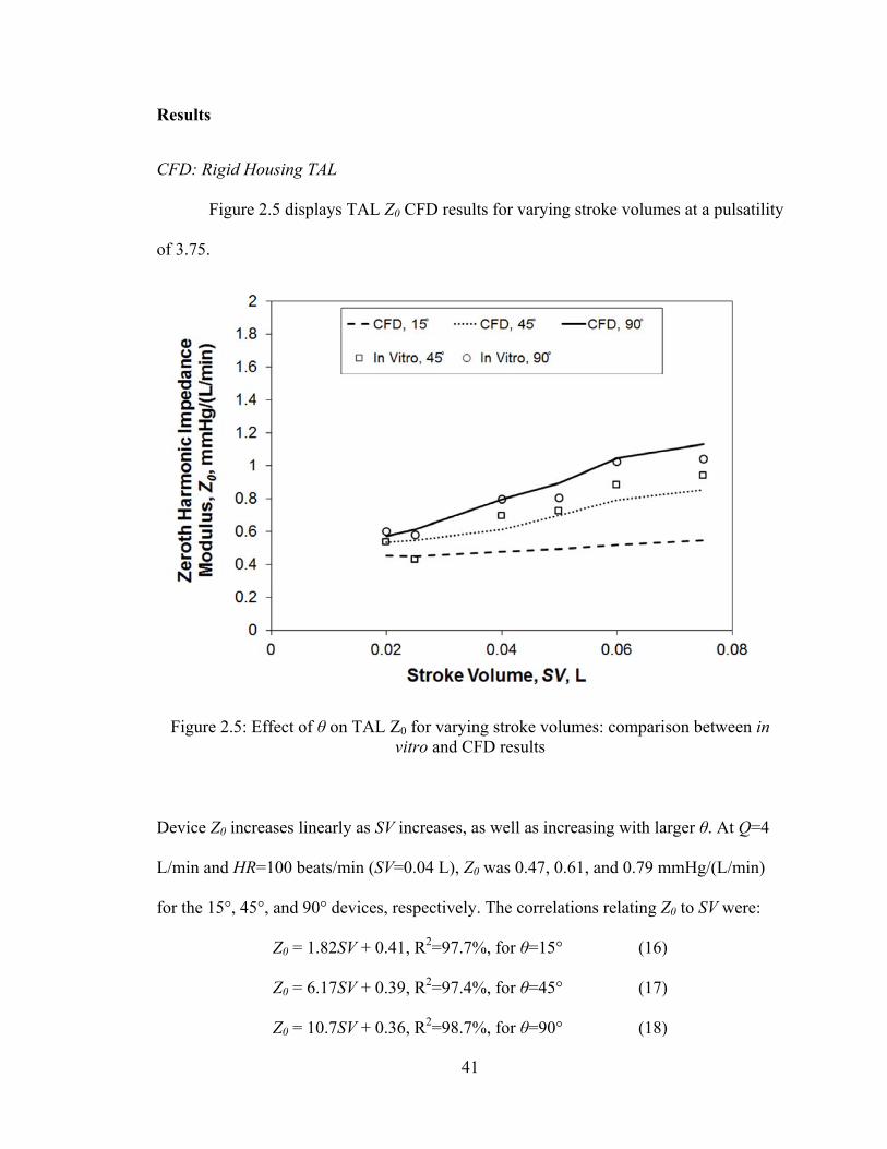
41

Results

CFD: Rigid Housing TAL

Figure 2.5 displays TAL Z0 CFD results for varying stroke volumes at a pulsatility

of 3.75.

Device Z0 increases linearly as SV increases, as well as increasing with larger θ. At Q=4

L/min and HR=100 beats/min (SV=0.04 L), Z0 was 0.47, 0.61, and 0.79 mmHg/(L/min)

for the 15°, 45°, and 90° devices, respectively. The correlations relating Z0 to SV were:

Z0 = 1.82SV + 0.41, R2=97.7%, for θ=15° (16)

Z0 = 6.17SV + 0.39, R2=97.4%, for θ=45° (17)

Z0 = 10.7SV + 0.36, R2=98.7%, for θ=90° (18)

Figure 2.5: Effect of θ on TAL Z0 for varying stroke volumes: comparison between in vitro and CFD results

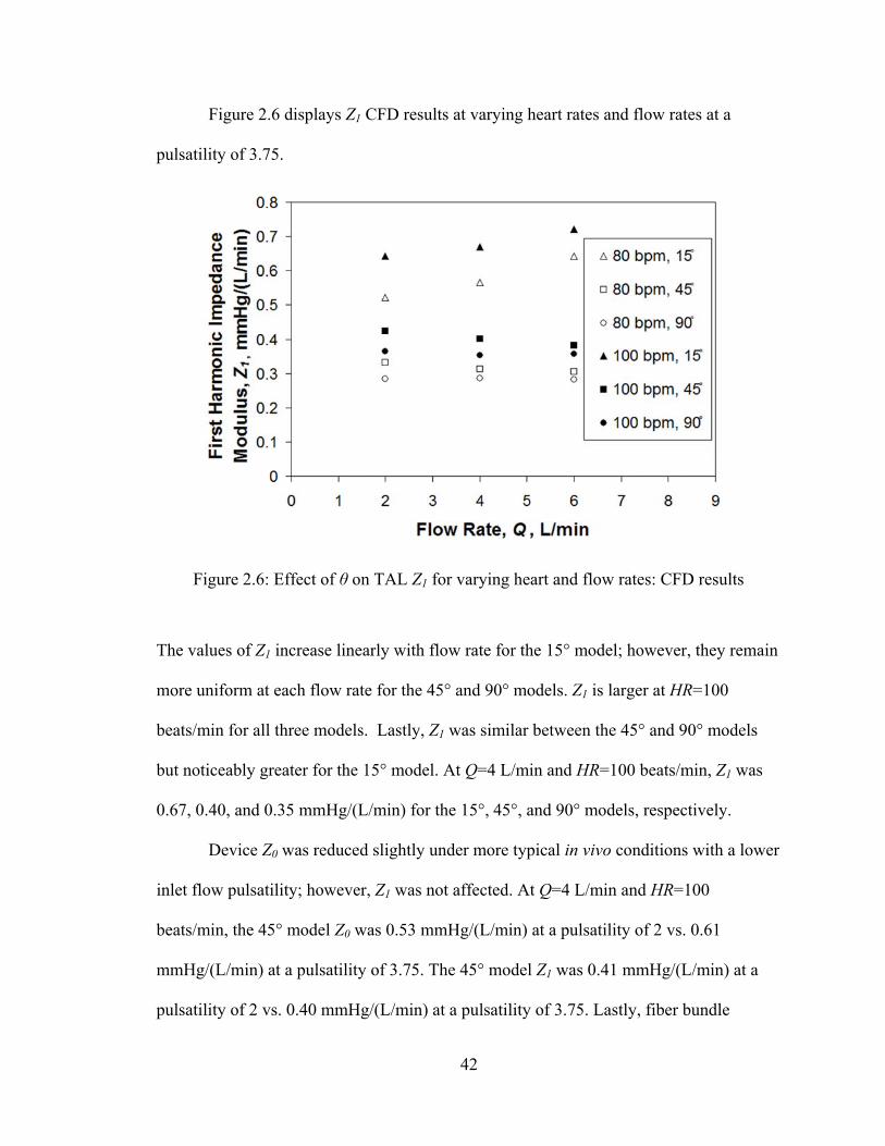
42

Figure 2.6 displays Z1 CFD results at varying heart rates and flow rates at a

pulsatility of 3.75.

The values of Z1 increase linearly with flow rate for the 15° model; however, they remain

more uniform at each flow rate for the 45° and 90° models. Z1 is larger at HR=100

beats/min for all three models. Lastly, Z1 was similar between the 45° and 90° models

but noticeably greater for the 15° model. At Q=4 L/min and HR=100 beats/min, Z1 was

0.67, 0.40, and 0.35 mmHg/(L/min) for the 15°, 45°, and 90° models, respectively.

Device Z0 was reduced slightly under more typical in vivo conditions with a lower

inlet flow pulsatility; however, Z1 was not affected. At Q=4 L/min and HR=100

beats/min, the 45° model Z0 was 0.53 mmHg/(L/min) at a pulsatility of 2 vs. 0.61

mmHg/(L/min) at a pulsatility of 3.75. The 45° model Z1 was 0.41 mmHg/(L/min) at a

pulsatility of 2 vs. 0.40 mmHg/(L/min) at a pulsatility of 3.75. Lastly, fiber bundle

Figure 2.6: Effect of θ on TAL Z1 for varying heart and flow rates: CFD results

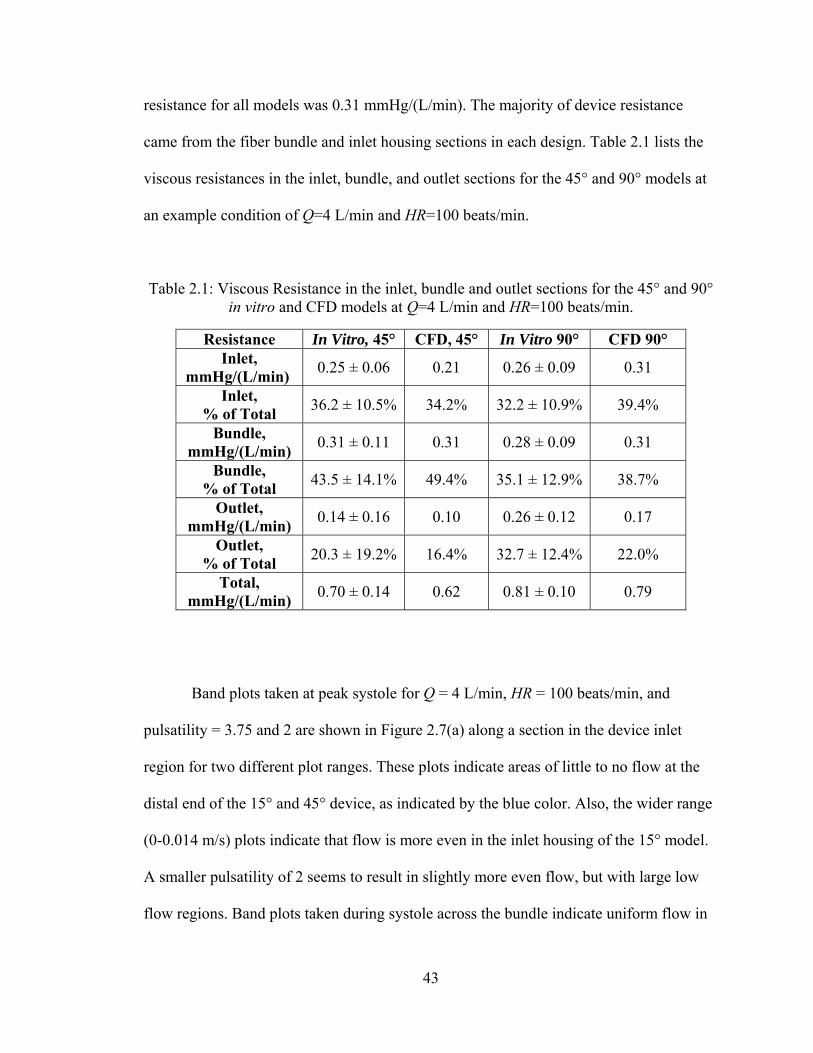
43

resistance for all models was 0.31 mmHg/(L/min). The majority of device resistance

came from the fiber bundle and inlet housing sections in each design. Table 2.1 lists the

viscous resistances in the inlet, bundle, and outlet sections for the 45° and 90° models at

an example condition of Q=4 L/min and HR=100 beats/min.

Table 2.1: Viscous Resistance in the inlet, bundle and outlet sections for the 45° and 90° in vitro and CFD models at Q=4 L/min and HR=100 beats/min.

Resistance In Vitro, 45° CFD, 45° In Vitro 90° CFD 90° Inlet,

mmHg/(L/min) 0.25 ± 0.06 0.21 0.26 ± 0.09 0.31

Inlet, % of Total

36.2 ± 10.5% 34.2% 32.2 ± 10.9% 39.4%

Bundle, mmHg/(L/min)

0.31 ± 0.11 0.31 0.28 ± 0.09 0.31

Bundle, % of Total

43.5 ± 14.1% 49.4% 35.1 ± 12.9% 38.7%

Outlet, mmHg/(L/min)

0.14 ± 0.16 0.10 0.26 ± 0.12 0.17

Outlet, % of Total

20.3 ± 19.2% 16.4% 32.7 ± 12.4% 22.0%

Total, mmHg/(L/min)

0.70 ± 0.14 0.62 0.81 ± 0.10 0.79

Band plots taken at peak systole for Q = 4 L/min, HR = 100 beats/min, and

pulsatility = 3.75 and 2 are shown in Figure 2.7(a) along a section in the device inlet

region for two different plot ranges. These plots indicate areas of little to no flow at the

distal end of the 15° and 45° device, as indicated by the blue color. Also, the wider range

(0-0.014 m/s) plots indicate that flow is more even in the inlet housing of the 15° model.

A smaller pulsatility of 2 seems to result in slightly more even flow, but with large low

flow regions. Band plots taken during systole across the bundle indicate uniform flow in

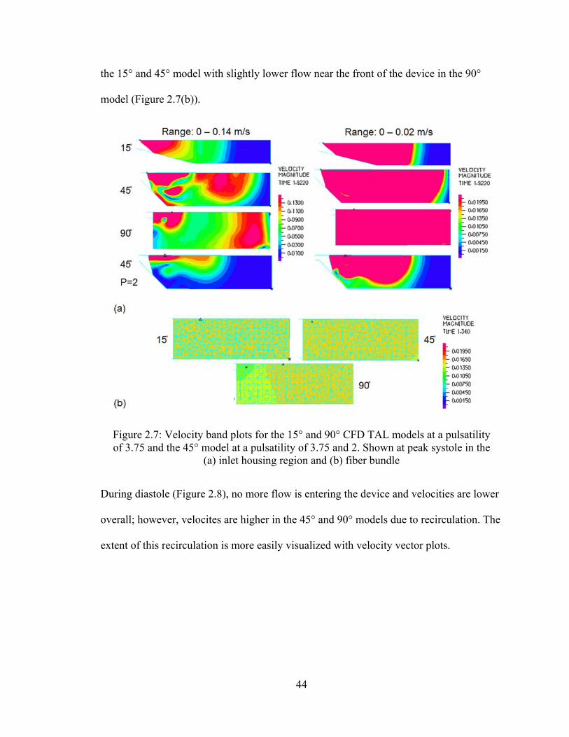
44

the 15° and 45° model with slightly lower flow near the front of the device in the 90°

model (Figure 2.7(b)).

During diastole (Figure 2.8), no more flow is entering the device and velocities are lower

overall; however, velocites are higher in the 45° and 90° models due to recirculation. The

extent of this recirculation is more easily visualized with velocity vector plots.

Figure 2.7: Velocity band plots for the 15° and 90° CFD TAL models at a pulsatility of 3.75 and the 45° model at a pulsatility of 3.75 and 2. Shown at peak systole in the

(a) inlet housing region and (b) fiber bundle

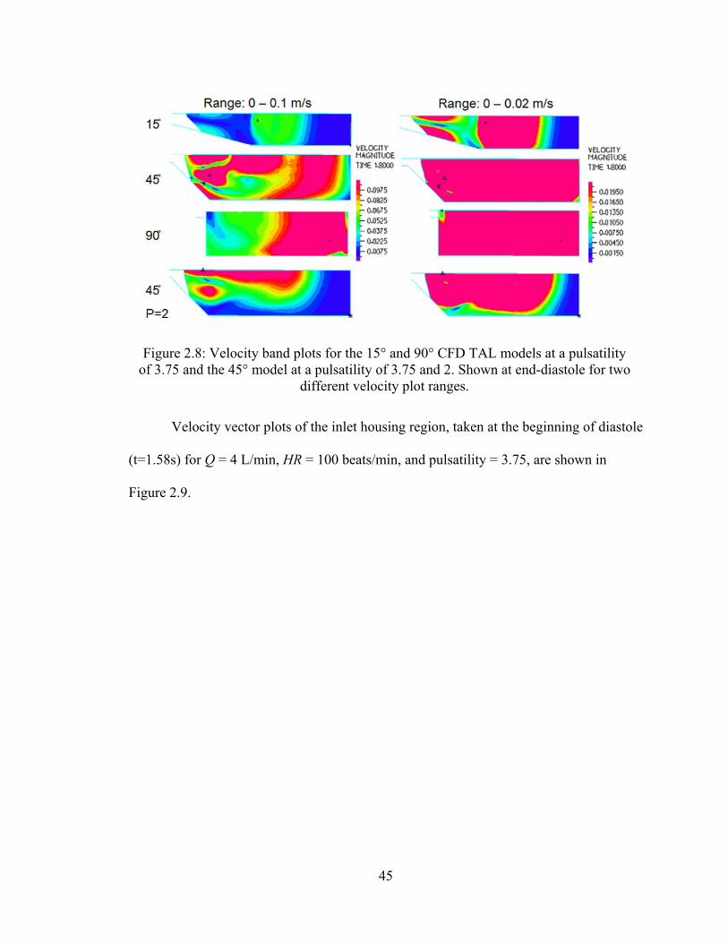
45

Velocity vector plots of the inlet housing region, taken at the beginning of diastole

(t=1.58s) for Q = 4 L/min, HR = 100 beats/min, and pulsatility = 3.75, are shown in

Figure 2.9.

Figure 2.8: Velocity band plots for the 15° and 90° CFD TAL models at a pulsatility of 3.75 and the 45° model at a pulsatility of 3.75 and 2. Shown at end-diastole for two

different velocity plot ranges.

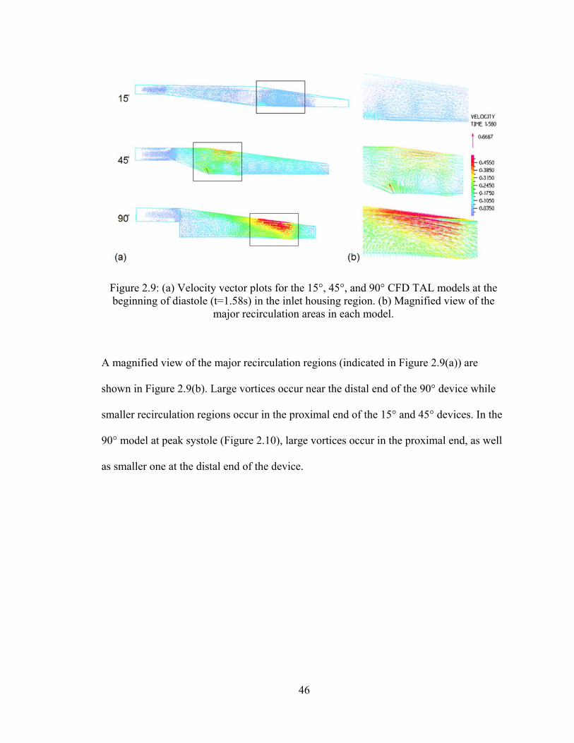
46

A magnified view of the major recirculation regions (indicated in Figure 2.9(a)) are

shown in Figure 2.9(b). Large vortices occur near the distal end of the 90° device while

smaller recirculation regions occur in the proximal end of the 15° and 45° devices. In the

90° model at peak systole (Figure 2.10), large vortices occur in the proximal end, as well

as smaller one at the distal end of the device.

Figure 2.9: (a) Velocity vector plots for the 15°, 45°, and 90° CFD TAL models at the beginning of diastole (t=1.58s) in the inlet housing region. (b) Magnified view of the

major recirculation areas in each model.

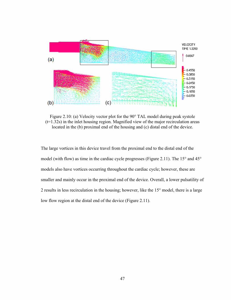
47

The large vortices in this device travel from the proximal end to the distal end of the

model (with flow) as time in the cardiac cycle progresses (Figure 2.11). The 15° and 45°

models also have vortices occurring throughout the cardiac cycle; however, these are

smaller and mainly occur in the proximal end of the device. Overall, a lower pulsatility of

2 results in less recirculation in the housing; however, like the 15° model, there is a large

low flow region at the distal end of the device (Figure 2.11).

Figure 2.10: (a) Velocity vector plot for the 90° TAL model during peak systole (t=1.32s) in the inlet housing region. Magnified view of the major recirculation areas

located in the (b) proximal end of the housing and (c) distal end of the device.

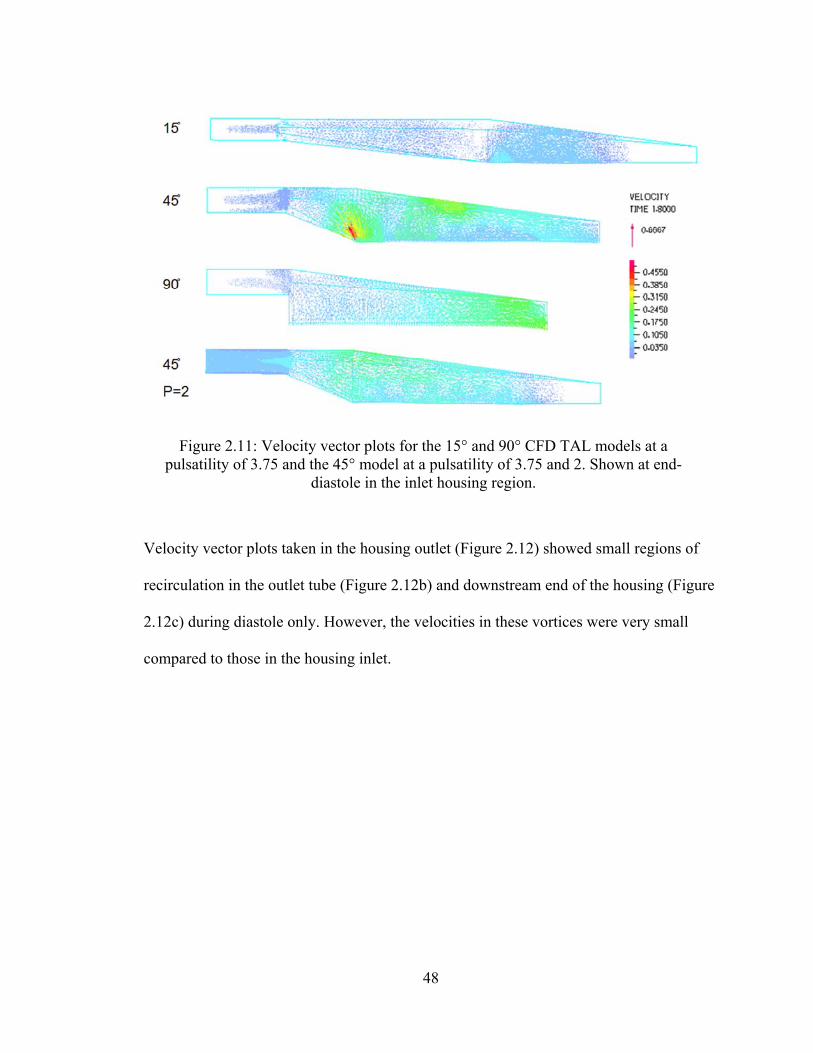
48

Velocity vector plots taken in the housing outlet (Figure 2.12) showed small regions of

recirculation in the outlet tube (Figure 2.12b) and downstream end of the housing (Figure

2.12c) during diastole only. However, the velocities in these vortices were very small

compared to those in the housing inlet.

Figure 2.11: Velocity vector plots for the 15° and 90° CFD TAL models at a pulsatility of 3.75 and the 45° model at a pulsatility of 3.75 and 2. Shown at end-

diastole in the inlet housing region.

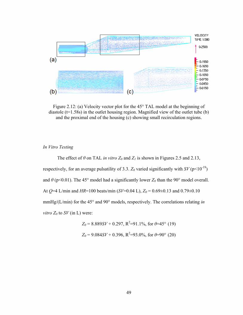
49

In Vitro Testing

The effect of θ on TAL in vitro Z0 and Z1 is shown in Figures 2.5 and 2.13,

respectively, for an average pulsatility of 3.3. Z0 varied significantly with SV (p<10-19)

and θ (p<0.01). The 45° model had a significantly lower Z0 than the 90° model overall.

At Q=4 L/min and HR=100 beats/min (SV=0.04 L), Z0 = 0.69±0.13 and 0.79±0.10

mmHg/(L/min) for the 45° and 90° models, respectively. The correlations relating in

vitro Z0 to SV (in L) were:

Z0 = 8.889SV + 0.297, R2=91.1%, for θ=45° (19)

Z0 = 9.084SV + 0.396, R2=93.0%, for θ=90° (20)

Figure 2.12: (a) Velocity vector plot for the 45° TAL model at the beginning of diastole (t=1.58s) in the outlet housing region. Magnified view of the outlet tube (b)

and the proximal end of the housing (c) showing small recirculation regions.

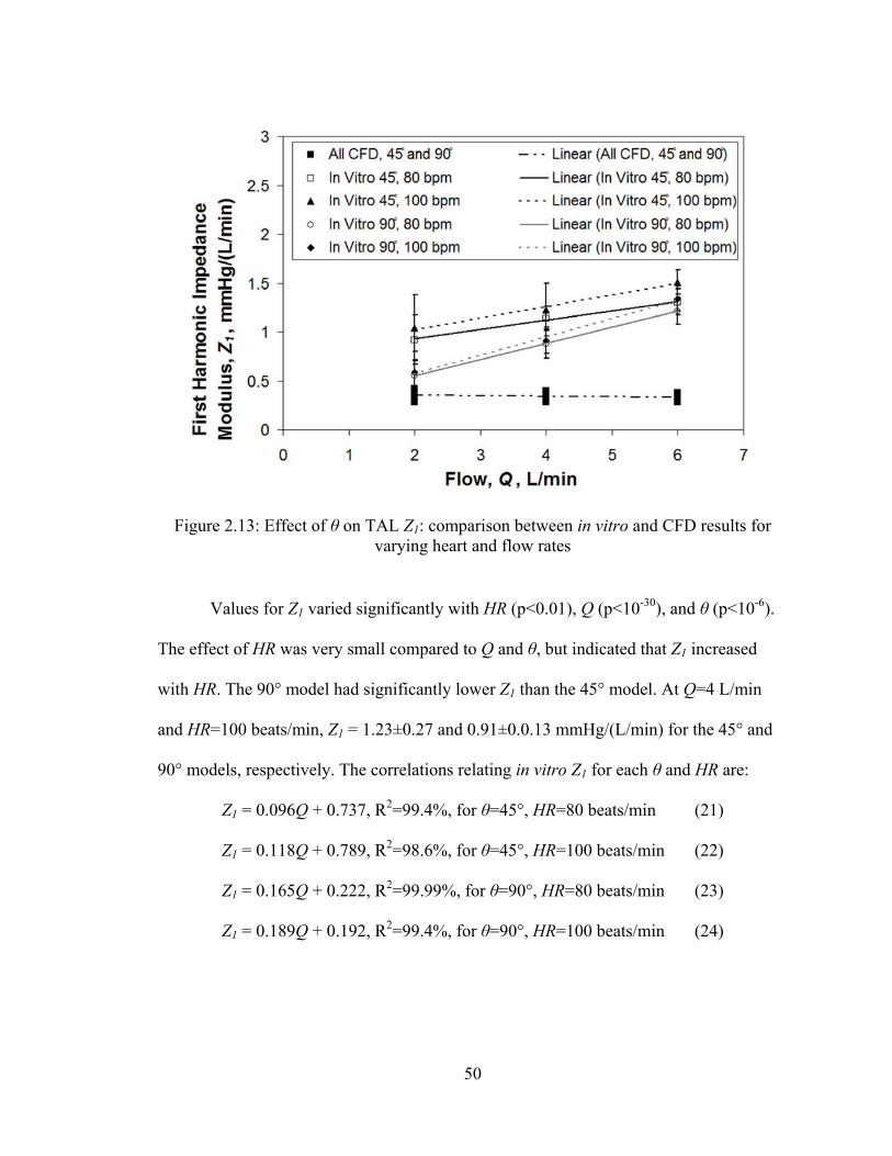
50

Values for Z1 varied significantly with HR (p<0.01), Q (p<10-30), and θ (p<10-6).

The effect of HR was very small compared to Q and θ, but indicated that Z1 increased

with HR. The 90° model had significantly lower Z1 than the 45° model. At Q=4 L/min

and HR=100 beats/min, Z1 = 1.23±0.27 and 0.91±0.0.13 mmHg/(L/min) for the 45° and

90° models, respectively. The correlations relating in vitro Z1 for each θ and HR are:

Z1 = 0.096Q + 0.737, R2=99.4%, for θ=45°, HR=80 beats/min (21)

Z1 = 0.118Q + 0.789, R2=98.6%, for θ=45°, HR=100 beats/min (22)

Z1 = 0.165Q + 0.222, R2=99.99%, for θ=90°, HR=80 beats/min (23)

Z1 = 0.189Q + 0.192, R2=99.4%, for θ=90°, HR=100 beats/min (24)

Figure 2.13: Effect of θ on TAL Z1: comparison between in vitro and CFD results for varying heart and flow rates

51

Overall, in vitro Z1 were larger and showed a stronger dependence on θ and Q than CFD

results. These larger Z1 were due to larger peak pressures in vitro, even though average

pressure drops were similar between the CFD and in vitro studies.

Average fiber bundle resistance for all models was 0.29 mmHg/(L/min), nearly

identical to CFD results. In the 45° model, the majority of device resistance came from

the fiber bundle and inlet housing sections. However, in the 90° model, the relative

contribution to total device resistance was almost identical for each section (Table 2.1).

Lastly, at a lower pulsatility of 1.7 with Q=4 L/min and HR=100 beats/min

(SV=0.04 L), the 45° model had Z0=0.65 mmHg/(L/min) and Z1=1.29 mmHg/(L/min).

The Z0 and Z1 are 0.69 and 1.23 mmHg/(L/min) at the same conditions with pulsatility

equal to 3.2. Therefore, as predicted in the CFD study, pulsatility does not greatly

influence impedance in vitro.

Discussion

The impedances of all the TAL designs tested in this study are significantly lower

than previous designs. Experiments with the MC3 Biolung (MC3, Ann Arbor, MI) [9] and

a cTAL [3] report Z0=1.8 and 1.9 mmHg/(L/min), respectively at 3.0 cP glycerol flows of

Q=4 L/min and HR=100 beats/min. At the same flow and heart rate, the 45° and 90°

model in the current study had Z0=0.69±0.13 and 0.79±0.10 mmHg/(L/min). These

values are also significantly lower than the impedance of the natural lung: Z0=1.25

mmHg/(L/min). Z1 in the healthy, natural lung is 0.49 mmHg/(L/min) [10] compared to

1.23 mmHg/(L/min) in the 45° model in this study.

52

The effect of SV and θ on Z0 was very similar in the CFD and in vitro results.

However, CFD modeling predicted lower Z1 values overall with a minimal effect of θ and

Q. The Z1 is more heavily influenced by differences in flow rate patterns and thus has a

higher variability than Z0 during in vitro testing. Overall, the Z1 values measured for both

models are small and unlikely to influence device function in vivo [11].

The 45° and 90° devices tested in this study had a 62 and 56% lower in vitro Z0

than previous designs. This decrease should improve RV function during attachment in

vivo. The ultimate effect of lower impedance on cardiac function depends on attachment

mode. The most likely clinical application for these devices is attachment in parallel with

the natural lung in a PA to left atrium (LA) configuration. If attached in parallel with the

natural lung, lower TAL impedance may allow patients to more easily exercise during

device attachment. Akay et al attached the MC3 Biolung in parallel with the pulmonary

circulation in sheep with chronic pulmonary hypertension and varied the percentage of

CO through the device under simulated rest, ambulatory, and exercise conditions [1]. At

ambulatory and resting conditions, CO was maintained as the percentage of CO to the

device increased. At exercise conditions, CO decreased with increasing flow to the TAL

up to 23 ± 5% at 90% flow diverted through the TAL. TAL impedance increases and the

natural lung impedance decreases with increasing blood flow. Thus, during exercise with

elevated CO, a higher percentage of CO may travel through the native lungs reducing

respiratory support when attached in parallel. Further decreases in device impedance may

allow for complete exercise tolerance and optimal device performance.

If attached in series with the natural lung, from the proximal to distal PA, lower

impedance should reduce the drop in CO that has been observed experimentally.

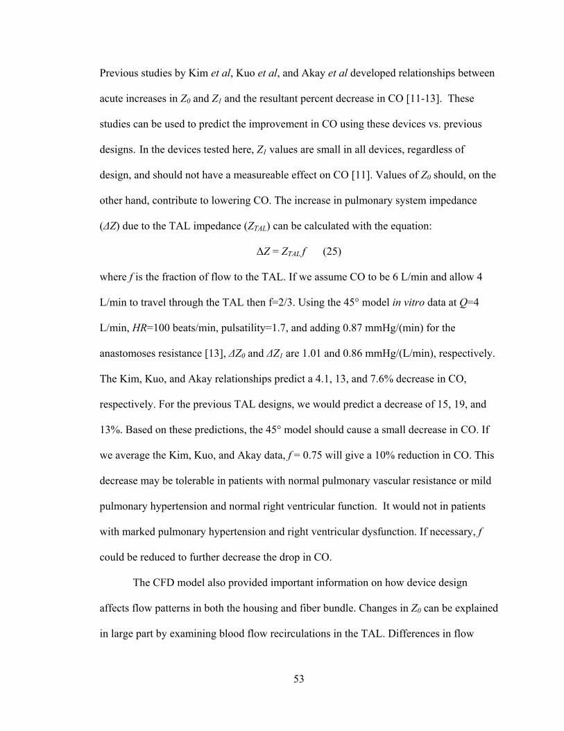
53

Previous studies by Kim et al, Kuo et al, and Akay et al developed relationships between

acute increases in Z0 and Z1 and the resultant percent decrease in CO [11-13]. These

studies can be used to predict the improvement in CO using these devices vs. previous

designs. In the devices tested here, Z1 values are small in all devices, regardless of

design, and should not have a measureable effect on CO [11]. Values of Z0 should, on the

other hand, contribute to lowering CO. The increase in pulmonary system impedance

(ΔZ) due to the TAL impedance (ZTAL) can be calculated with the equation:

ΔZ = ZTAL f (25)

where f is the fraction of flow to the TAL. If we assume CO to be 6 L/min and allow 4

L/min to travel through the TAL then f=2/3. Using the 45° model in vitro data at Q=4

L/min, HR=100 beats/min, pulsatility=1.7, and adding 0.87 mmHg/(min) for the

anastomoses resistance [13], ΔZ0 and ΔZ1 are 1.01 and 0.86 mmHg/(L/min), respectively.

The Kim, Kuo, and Akay relationships predict a 4.1, 13, and 7.6% decrease in CO,

respectively. For the previous TAL designs, we would predict a decrease of 15, 19, and

13%. Based on these predictions, the 45° model should cause a small decrease in CO. If

we average the Kim, Kuo, and Akay data, f = 0.75 will give a 10% reduction in CO. This

decrease may be tolerable in patients with normal pulmonary vascular resistance or mild

pulmonary hypertension and normal right ventricular function. It would not in patients

with marked pulmonary hypertension and right ventricular dysfunction. If necessary, f

could be reduced to further decrease the drop in CO.

The CFD model also provided important information on how device design

affects flow patterns in both the housing and fiber bundle. Changes in Z0 can be explained

in large part by examining blood flow recirculations in the TAL. Differences in flow

54

patterns were more pronounced in the housing inlet. The fiber bundle acted to evenly

distribute blood flow, resulting in more even blood flow in the housing outlet and only

small, low-velocity, recirculations. Recirculation occurred in the inlet of all three models;

however, recirculations decreased as θ decreased. The 90° housing inlet had several

regions of large vortices throughout the cardiac cycle, while the 15° and 45° models had

smaller areas of recirculation.

Device design also affected flow uniformity in the housing inlet and fiber bundle.

Flow uniformity is essential to the short and long-term function of the device. Regions of

little or no flow offer little gas exchange when they occur in the fiber bundle and, worse

yet, can lead to a buildup of activated clotting factors and clot formation when they

occur at any of the device artificial surfaces. The 15° and 45° models had areas of little to

no flow near the distal end of the inlet. These areas were larger in the 15° model where

flow was barely reaching past the middle of the housing body. The stasis regions in the

back of the device can never completely be eliminated for the angled housings, but

further geometry changes may help, such as a shorter distance between the inlet and the

back and tapered corners in the back. Tapered corners are easily incorporated during the

production process when the fiber bundle is “potted” in urethane to separate the blood

and gas phases of the device.

Ultimately, the optimal device must have a combination of low impedance, even

flow, and reasonable size for use by an ambulatory patient. While the 15° model had

smaller recirculation regions and low impedance, it had a large stasis region near the

distal end of the device. Also, the long inlet and outlet length of the 15° model may make

it unwieldy to use with patients. Therefore, the 45° model has the optimal combination

55

of low impedance, better flow patterns, and relatively compact size. The low impedance

of the 45° model should allow for a minimal, acute decrease in CO at rest if implanted in

series with the natural lung and increased exercise tolerance when compared to previous

TAL designs if attached in parallel with high flows to the TAL. These results will be

confirmed by examining compliant housing models, discussed in the following chapters.

56

References

1. Akay B, Reoma JL, Camboni D, et al. In-parallel artificial lung attachment at

high flows in normal and pulmonary hypertension models. Ann Thorac Surg 90:

259-65, 2010

2. Sato H, McGillicuddy JH, Griffith GW, et al. Effect of artificial lung compliance

on in vivo pulmonary system hemodynamics. ASAIO J 52: 248-256, 2006.

3. Cook KE, Perlman CE, Seipelt R, et al. Hemodynamic and gas transfer properties

of a compliant thoracic artificial lung. ASAIO J 51: 404-411, 2005.

4. Funakubo A, Taga I, McGillicuddy JW, et al. Flow vectorial analysis in an

artificial implantable lung. ASAIO J 49(4): 383-7, 2003.

5. Gage KL, Gartner MJ, Burgreen GW, Wagner WR. Predicting membrane

oxygenator pressure drop using computational fluid dynamics Artificial Organs

26 (7): 600-607, 2002.

6. Matsuda N, Nakamura M, Sakai K, Kuwana K. Theoretical and experimental

evaluation for blood pressure drop and oxygen transfer rate in outside blood flow

membrane oxygenator. J. Chemical Engineering of Japan 32 (6): 752-759, 1999.

7. Taga I, Funakubo A, Fukui Y. Design and development of an artificial

implantable lung using multiobjective genetic algorithm: evaluation of gas

exchange performance. ASAIO J 51(1): 92-102, 2005.

8. Van Grondelle A. Analysis of pulmonary arterial blood flow dynamics with

special reference to congenital heart disease. Evanston, IL: Northwestern

University; 1982. Thesis.

57

9. McGillicuddy JW, Chambers SD, Galligan DT, et al. In vitro fluid mechanical

effects of thoracic artificial lung compliance. ASAIO J 51: 789-794, 2005.

10. Laskey WK, Ferrari VA, Palevsky HI, Kussmaul WG. Pulmonary artery

hemodynamics in primary pulmonary hypertension. J Am Coll Cardiol 21: 406-

12, 1993.

11. Kuo AS, Sato H, Reoma JL, Cook KE. The relationship between pulmonary

system impedance and right ventricular function in normal sheep. Cardiovascular

Engineering 9: 153-160, 2009.

12. Kim J, Sato H, Griffith GW, Cook KE. Cardiac output during high afterload

artificial lung attachment. ASAIO J 55: 73-77, 2009.

13. Akay B, Foucher JA, Camboni D, Koch KL, Kawatra A, Cook KE.

Hemodynamic design requirements for in series thoracic artificial lung attachment

in a model of pulmonary hypertension. ASAIO Journal, Epub ahead of print.

58

Chapter 3

Compliant Thoracic Artificial Lung Design and Testing

Introduction

CFD and in vitro studies with a rigid-housing TAL showed that device impedance

was reduced as the inlet and outlet expansion angle, θ, decreased. The optimum

combination of low impedance and good flow patterns was achieved with the 45°

housing model. Now we will confirm these results and investigate whether additional

reductions in TAL impedance may be achieved by using a compliant housing material.

Unlike a hard-shell TAL, the compliant housing can expand to accommodate the large

changes in blood volume seen during a heartbeat. This dampens the flow pulse, creating a

more steady flow through the cardiac cycle.

This study aimed to reduce TAL impedance using a compliant housing material in

conjunction with more gradual inlet and outlet geometries, as explored in Chapter 2. In

this compliant thoracic artificial lung (cTAL), blood flows through the inlet and into the

compliant inlet manifold (Figure 2.1). The housing expands, accommodating the stroke

volume without a large pressure increase. Blood then flows through the fiber bundle

where gas exchange occurs, through the bottom housing manifold and finally exits

through the outlet. The effect of inlet and outlet expansion angle, θ, on cTAL impedance

and flow patterns was explored with fluid-structure interaction (FSI) analysis. The FSI

59

analysis was necessary to examine the interaction between fluid forces and housing

deformation. The optimal cTAL design was determined from FSI results, prototyped, and

tested in vitro to assess impedance and gas transfer performance.

Methods

Fluid Structure Interaction Analysis

SolidWorks was used to create cTAL models with varying housing geometries

using θ= 15°, 45°, and 90° (Figures 2.1 and 2.2). The inlet/outlet diameter, height, and

width of each cTAL model are 0.016 m, 0.103 m, and 0.102 m, respectively. The fiber

bundle length, path length, and frontal area are 0.127 m, 0.038 m, and 0.013 m2,

respectively, for each model. The 15°, 45°, and 90° models have a total length of 0.338,

0.221 m, and 0.178 m. These models were then imported into ADINA. For FSI analysis,

separate structure and fluid models were created, coupled and then run together. The fluid

model consisted of all regions that fluid passed through while the structure model

consisted of the Biospan housing.

FSI: Problem Formulation

Program assumptions included a transient solution with incompressible flow. At a

flow of 3 L/min, the Reynolds number during peak flow was 4150 in the inlet section,

170 coming out of the bundle into the outlet section, and 3300 exiting the device. Due to

limitations in the CFD software, we could not apply turbulent flow to the fiber bundle

(porous media model). This required us to split up sections and run their simulations

60

independently, while carrying boundary conditions from one section to the next. Two

such solutions were attempted: i) running each section independently, with turbulence in

the inlet and outlet sections and laminar flow in the bundle (as done for TAL models in

Chapter 2), and ii) running the inlet section as turbulent and remainder of the model as

laminar. The former gave unrealistic flow patterns and dampening (detailed further in

discussion). The latter gave us the most quantitatively accurate and physically realistic

results possible and is thus presented here.

In the fluid model, the properties of the fiber bundle and the fluid characteristics

of blood were defined as described in the TAL CFD study (Chapter 2). A slip wall

boundary condition was applied to the bundle walls while a FSI condition was used in the

inlet and outlet regions. A pressure of 770 mmHg (absolute pressure) was applied at the

outlet and also used for the initial pressure condition. A time dependent velocity was

applied to the inlet face using the same pulsatile flow waveform (as described in Chapter

2) with average flow rates, Q, of 3 and 5 L/min and a heart rate, HR, of 100 beats/min.

The structure model consisted of the compliant, Biospan (DSM PTG, Berkeley,

CA) housing, with a thickness of 0.51 mm, forming the inlet and outlet sections of the

model. Biospan was defined as an elastic isotropic material with a Young’s modulus of

6.21 MPa, Poisson’s ratio of 0.40, and density of 1030 kg/m3. FSI boundary conditions

were applied to each face and shell elements were used with a face thickness of 0.51 mm.

The edges bordering the fiber bundle were fixed in all directions, along with the inlet and

outlet edge to prevent translation of the model in space. Symmetry plane edges were

fixed in the direction normal to the symmetry plane. Atmospheric pressure was applied to

61

the model by applying a pressure load of 760 mmHg to the exterior faces of the structure

model.

The governing equations used for the problem formulation in the fluid domain are

the continuity and Navier-Stokes equations:

Bff fσuuu

u

u

fgff t

0

(1)

where u is the fluid velocity vector, f is the fluid density, ug is the moving coordinate

velocity, Bff is the body force per unit volume, guu is the relative velocity of the

fluid with respect to the moving coordinate velocity, and f is the fluid stress tensor.

The governing equation for the solid domain of the FSI model is the

elastodynamics equation:

Bssss fσd (2)

where s is the wall density, s is the solid Cauchy stress tensor, Bsf is the externally

applied body force vector at time t and sd represents the local acceleration of the solid

region ( guds ).

The boundary conditions at the interface between the fluid domain and the solid

domain are:

guu

sσfσ

sdfd

:slip-No

:Traction

:ntDisplaceme

(3)

where d, , n are the displacement vector, stress tensor, and normal vector, respectively.

The subscripts s and f indicate fluid and solid properties, respectively.

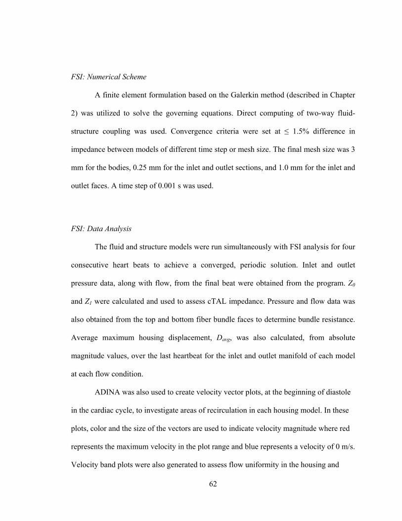
62

FSI: Numerical Scheme

A finite element formulation based on the Galerkin method (described in Chapter

2) was utilized to solve the governing equations. Direct computing of two-way fluid-

structure coupling was used. Convergence criteria were set at ≤ 1.5% difference in

impedance between models of different time step or mesh size. The final mesh size was 3

mm for the bodies, 0.25 mm for the inlet and outlet sections, and 1.0 mm for the inlet and

outlet faces. A time step of 0.001 s was used.

FSI: Data Analysis

The fluid and structure models were run simultaneously with FSI analysis for four

consecutive heart beats to achieve a converged, periodic solution. Inlet and outlet

pressure data, along with flow, from the final beat were obtained from the program. Z0

and Z1 were calculated and used to assess cTAL impedance. Pressure and flow data was

also obtained from the top and bottom fiber bundle faces to determine bundle resistance.

Average maximum housing displacement, Davg, was also calculated, from absolute

magnitude values, over the last heartbeat for the inlet and outlet manifold of each model

at each flow condition.

ADINA was also used to create velocity vector plots, at the beginning of diastole

in the cardiac cycle, to investigate areas of recirculation in each housing model. In these

plots, color and the size of the vectors are used to indicate velocity magnitude where red

represents the maximum velocity in the plot range and blue represents a velocity of 0 m/s.

Velocity band plots were also generated to assess flow uniformity in the housing and

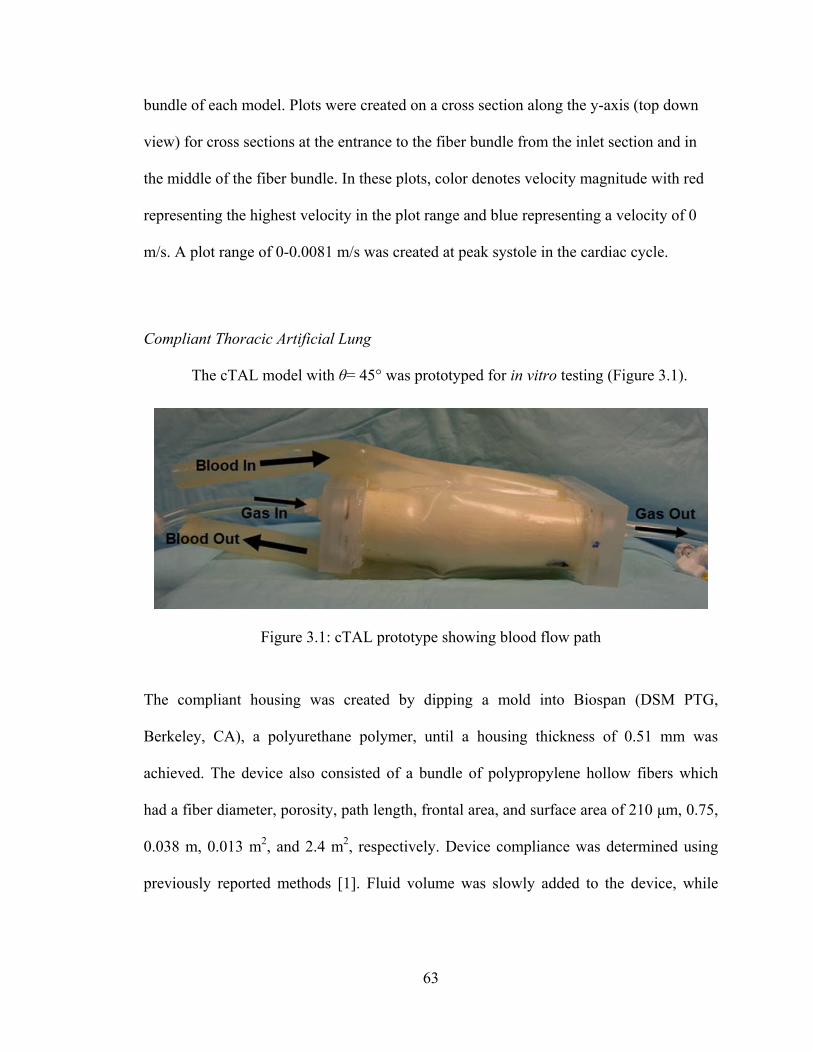
63

bundle of each model. Plots were created on a cross section along the y-axis (top down

view) for cross sections at the entrance to the fiber bundle from the inlet section and in

the middle of the fiber bundle. In these plots, color denotes velocity magnitude with red

representing the highest velocity in the plot range and blue representing a velocity of 0

m/s. A plot range of 0-0.0081 m/s was created at peak systole in the cardiac cycle.

Compliant Thoracic Artificial Lung

The cTAL model with θ= 45° was prototyped for in vitro testing (Figure 3.1).

The compliant housing was created by dipping a mold into Biospan (DSM PTG,

Berkeley, CA), a polyurethane polymer, until a housing thickness of 0.51 mm was

achieved. The device also consisted of a bundle of polypropylene hollow fibers which

had a fiber diameter, porosity, path length, frontal area, and surface area of 210 μm, 0.75,

0.038 m, 0.013 m2, and 2.4 m2, respectively. Device compliance was determined using

previously reported methods [1]. Fluid volume was slowly added to the device, while

Figure 3.1: cTAL prototype showing blood flow path

64

pressure was recorded and compliance was calculated as ΔV/ΔP, until an added fluid

volume of 560 mL was reached.

In Vitro Testing: Hemodynamics

In vitro testing was conducted in a circuit consisting of a pulsatile pump (Harvard

Apparatus, Holliston, MA), cTAL (n = 4), and reservoir filled with 3.0 cP glycerol

solution (Figure 3.2a). The reservoir was raised 12.6 cm above the cTAL outlet, resulting

in a constant device outlet pressure of 10 mmHg. Fluid-coupled pressure transducers

(Abbott Critical Care Systems, Chicago, IL) measured pressure at the cTAL inlet (Pi) and

outlet (Po). A flow probe (14PXL, Transonic Systems Inc, Ithaca, NY) measured the flow

rate into the cTAL (QcTAL).

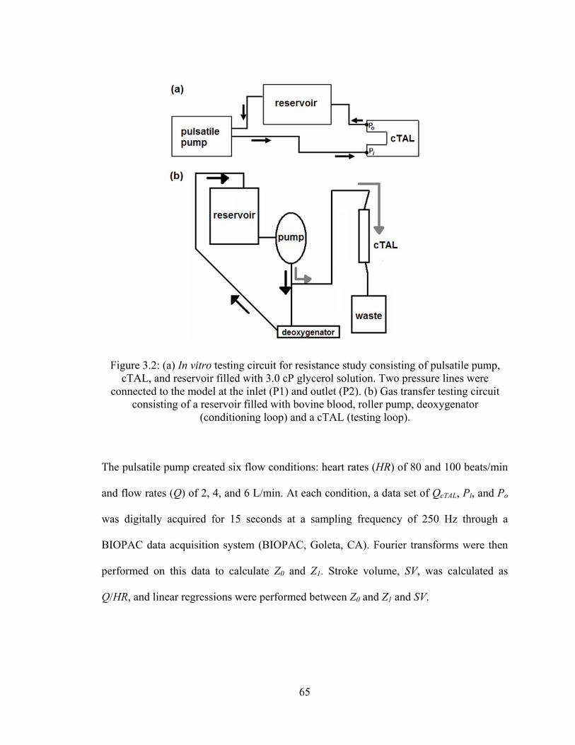
65

The pulsatile pump created six flow conditions: heart rates (HR) of 80 and 100 beats/min

and flow rates (Q) of 2, 4, and 6 L/min. At each condition, a data set of QcTAL, Pi, and Po

was digitally acquired for 15 seconds at a sampling frequency of 250 Hz through a

BIOPAC data acquisition system (BIOPAC, Goleta, CA). Fourier transforms were then

performed on this data to calculate Z0 and Z1. Stroke volume, SV, was calculated as

Q/HR, and linear regressions were performed between Z0 and Z1 and SV.

Figure 3.2: (a) In vitro testing circuit for resistance study consisting of pulsatile pump, cTAL, and reservoir filled with 3.0 cP glycerol solution. Two pressure lines were

connected to the model at the inlet (P1) and outlet (P2). (b) Gas transfer testing circuit consisting of a reservoir filled with bovine blood, roller pump, deoxygenator

(conditioning loop) and a cTAL (testing loop).

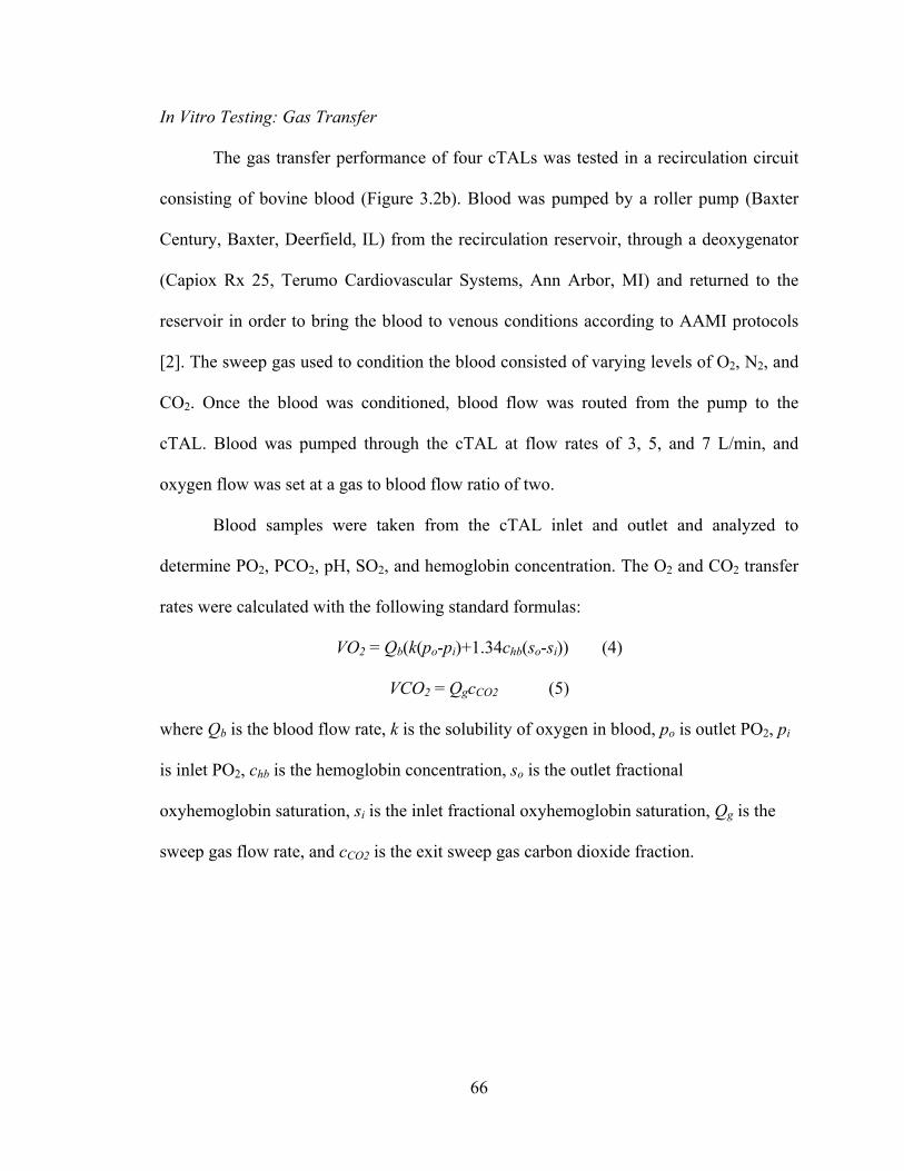
66

In Vitro Testing: Gas Transfer

The gas transfer performance of four cTALs was tested in a recirculation circuit

consisting of bovine blood (Figure 3.2b). Blood was pumped by a roller pump (Baxter

Century, Baxter, Deerfield, IL) from the recirculation reservoir, through a deoxygenator

(Capiox Rx 25, Terumo Cardiovascular Systems, Ann Arbor, MI) and returned to the

reservoir in order to bring the blood to venous conditions according to AAMI protocols

[2]. The sweep gas used to condition the blood consisted of varying levels of O2, N2, and

CO2. Once the blood was conditioned, blood flow was routed from the pump to the

cTAL. Blood was pumped through the cTAL at flow rates of 3, 5, and 7 L/min, and

oxygen flow was set at a gas to blood flow ratio of two.

Blood samples were taken from the cTAL inlet and outlet and analyzed to

determine PO2, PCO2, pH, SO2, and hemoglobin concentration. The O2 and CO2 transfer

rates were calculated with the following standard formulas:

VO2 = Qb(k(po-pi)+1.34chb(so-si)) (4)

VCO2 = QgcCO2 (5)

where Qb is the blood flow rate, k is the solubility of oxygen in blood, po is outlet PO2, pi

is inlet PO2, chb is the hemoglobin concentration, so is the outlet fractional

oxyhemoglobin saturation, si is the inlet fractional oxyhemoglobin saturation, Qg is the

sweep gas flow rate, and cCO2 is the exit sweep gas carbon dioxide fraction.

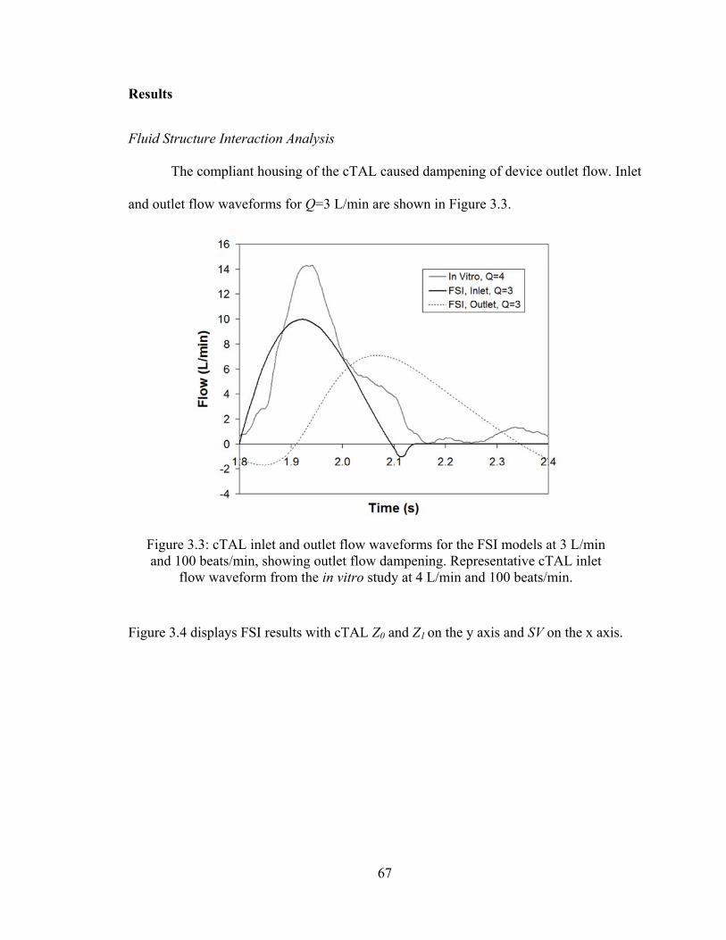
67

Results

Fluid Structure Interaction Analysis

The compliant housing of the cTAL caused dampening of device outlet flow. Inlet

and outlet flow waveforms for Q=3 L/min are shown in Figure 3.3.

Figure 3.4 displays FSI results with cTAL Z0 and Z1 on the y axis and SV on the x axis.

Figure 3.3: cTAL inlet and outlet flow waveforms for the FSI models at 3 L/min and 100 beats/min, showing outlet flow dampening. Representative cTAL inlet

flow waveform from the in vitro study at 4 L/min and 100 beats/min.

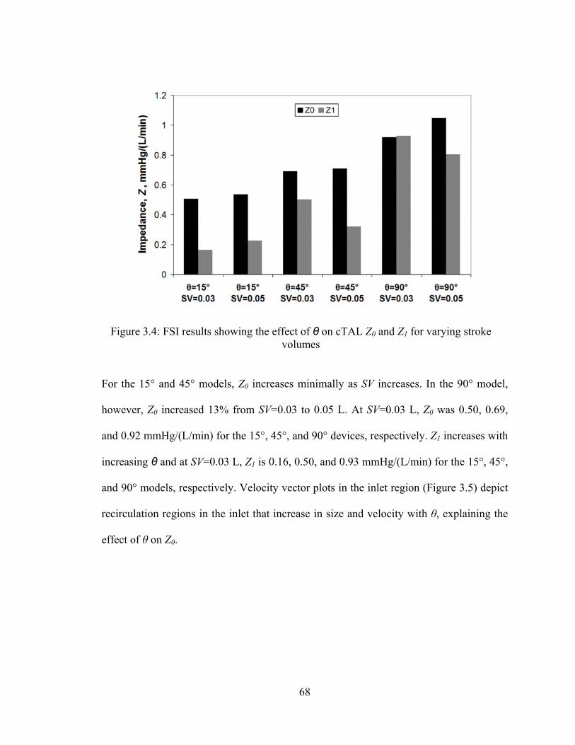
68

For the 15° and 45° models, Z0 increases minimally as SV increases. In the 90° model,

however, Z0 increased 13% from SV=0.03 to 0.05 L. At SV=0.03 L, Z0 was 0.50, 0.69,

and 0.92 mmHg/(L/min) for the 15°, 45°, and 90° devices, respectively. Z1 increases with

increasing θ and at SV=0.03 L, Z1 is 0.16, 0.50, and 0.93 mmHg/(L/min) for the 15°, 45°,

and 90° models, respectively. Velocity vector plots in the inlet region (Figure 3.5) depict

recirculation regions in the inlet that increase in size and velocity with θ, explaining the

effect of θ on Z0.

Figure 3.4: FSI results showing the effect of θ on cTAL Z0 and Z1 for varying stroke volumes

69

Velocity band plots taken at cross sections in the inlet region at the entrance to the

fiber bundle (Figure 3.6a) and the middle of the fiber bundle (Figure 3.6b) are shown in

Figure 3.6.

Figure 3.5: (a) Velocity vector plots for the 15°, 45°, and 90° cTAL models at the beginning of diastole (t=2.14s) in the inlet housing region. (b) Magnified view of the

major recirculation areas in each model.

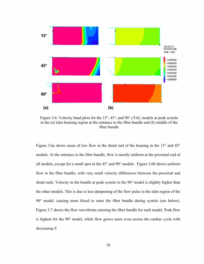
70

Figure 3.6a shows areas of low flow in the distal end of the housing in the 15° and 45°

models. At the entrance to the fiber bundle, flow is mostly uniform at the proximal end of

all models, except for a small spot in the 45° and 90° models. Figure 3.6b shows uniform

flow in the fiber bundle, with very small velocity differences between the proximal and

distal ends. Velocity in the bundle at peak systole in the 90° model is slightly higher than

the other models. This is due to less dampening of the flow pulse in the inlet region of the

90° model, causing more blood to enter the fiber bundle during systole (see below).

Figure 3.7 shows the flow waveforms entering the fiber bundle for each model. Peak flow

is highest for the 90° model, while flow grows more even across the cardiac cycle with

decreasing θ.

Figure 3.6: Velocity band plots for the 15°, 45°, and 90° cTAL models at peak systole in the (a) inlet housing region at the entrance to the fiber bundle and (b) middle of the

fiber bundle

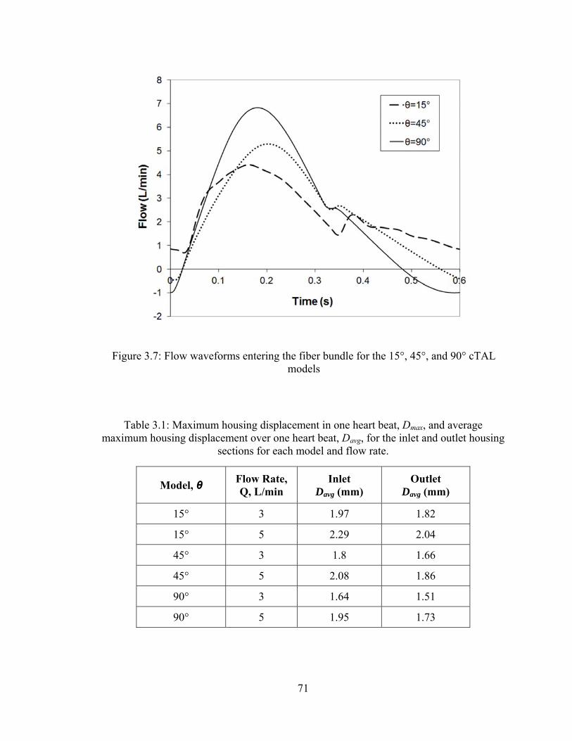
71

Table 3.1: Maximum housing displacement in one heart beat, Dmax, and average maximum housing displacement over one heart beat, Davg, for the inlet and outlet housing

sections for each model and flow rate.

Model, θ Flow Rate, Q, L/min

Inlet Davg (mm)

Outlet Davg (mm)

15° 3 1.97 1.82

15° 5 2.29 2.04

45° 3 1.8 1.66

45° 5 2.08 1.86

90° 3 1.64 1.51

90° 5 1.95 1.73

Figure 3.7: Flow waveforms entering the fiber bundle for the 15°, 45°, and 90° cTAL models

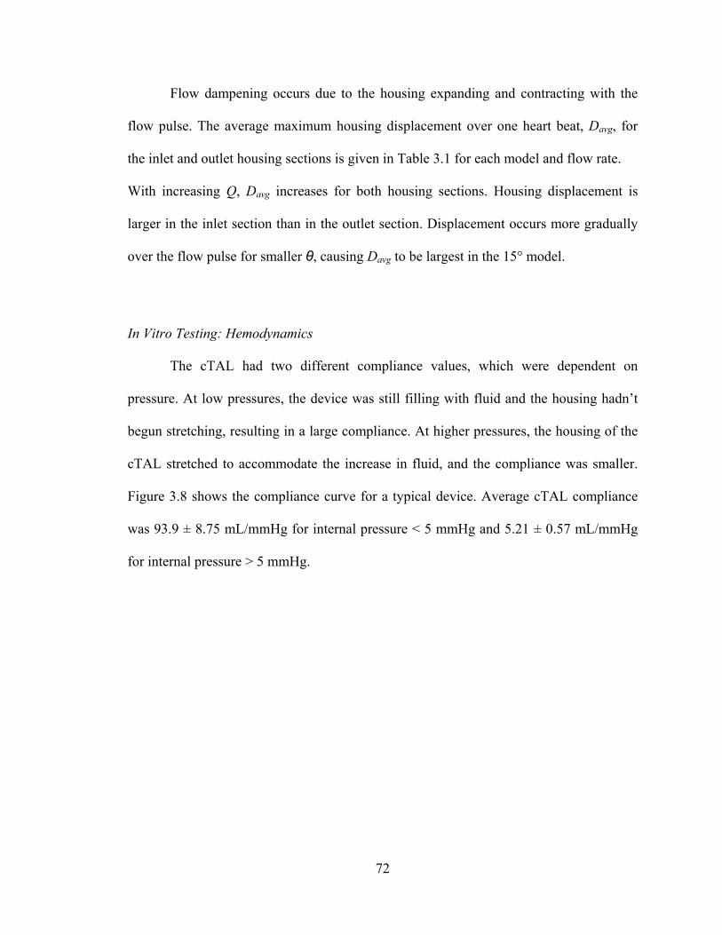
72

Flow dampening occurs due to the housing expanding and contracting with the

flow pulse. The average maximum housing displacement over one heart beat, Davg, for

the inlet and outlet housing sections is given in Table 3.1 for each model and flow rate.

With increasing Q, Davg increases for both housing sections. Housing displacement is

larger in the inlet section than in the outlet section. Displacement occurs more gradually

over the flow pulse for smaller θ, causing Davg to be largest in the 15° model.

In Vitro Testing: Hemodynamics

The cTAL had two different compliance values, which were dependent on

pressure. At low pressures, the device was still filling with fluid and the housing hadn’t

begun stretching, resulting in a large compliance. At higher pressures, the housing of the

cTAL stretched to accommodate the increase in fluid, and the compliance was smaller.

Figure 3.8 shows the compliance curve for a typical device. Average cTAL compliance

was 93.9 ± 8.75 mL/mmHg for internal pressure < 5 mmHg and 5.21 ± 0.57 mL/mmHg

for internal pressure > 5 mmHg.

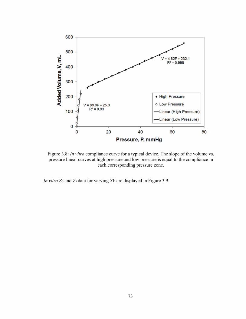
73

In vitro Z0 and Z1 data for varying SV are displayed in Figure 3.9.

Figure 3.8: In vitro compliance curve for a typical device. The slope of the volume vs. pressure linear curves at high pressure and low pressure is equal to the compliance in

each corresponding pressure zone.

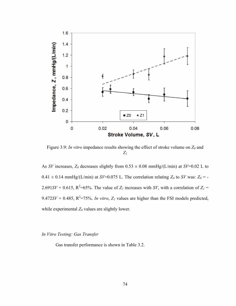
74

As SV increases, Z0 decreases slightly from 0.53 ± 0.08 mmHg/(L/min) at SV=0.02 L to

0.41 ± 0.14 mmHg/(L/min) at SV=0.075 L. The correlation relating Z0 to SV was: Z0 = -

2.691SV + 0.615, R2=65%. The value of Z1 increases with SV, with a correlation of Z1 =

9.472SV + 0.485, R2=75%. In vitro, Z1 values are higher than the FSI models predicted,

while experimental Z0 values are slightly lower.

In Vitro Testing: Gas Transfer

Gas transfer performance is shown in Table 3.2.

Figure 3.9: In vitro impedance results showing the effect of stroke volume on Z0 and Z1

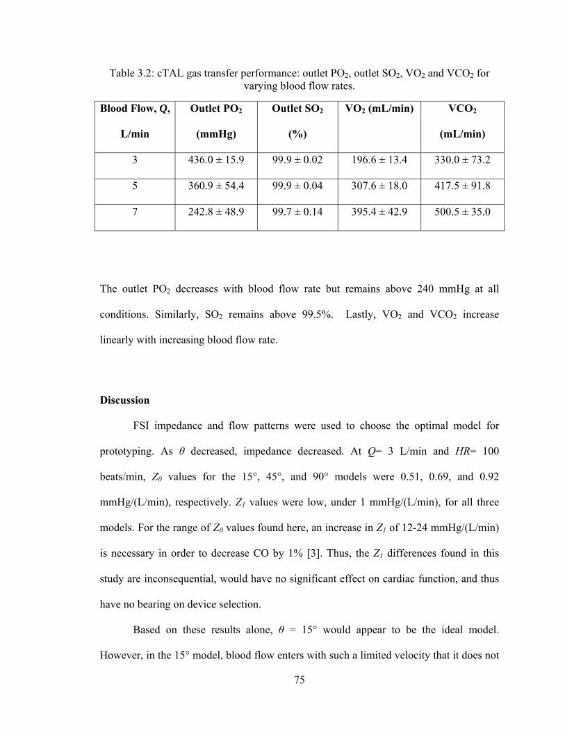
75

Table 3.2: cTAL gas transfer performance: outlet PO2, outlet SO2, VO2 and VCO2 for varying blood flow rates.

Blood Flow, Q,

L/min

Outlet PO2

(mmHg)

Outlet SO2

(%)

VO2 (mL/min) VCO2

(mL/min)

3 436.0 ± 15.9 99.9 ± 0.02 196.6 ± 13.4 330.0 ± 73.2

5 360.9 ± 54.4 99.9 ± 0.04 307.6 ± 18.0 417.5 ± 91.8

7 242.8 ± 48.9 99.7 ± 0.14 395.4 ± 42.9 500.5 ± 35.0

The outlet PO2 decreases with blood flow rate but remains above 240 mmHg at all

conditions. Similarly, SO2 remains above 99.5%. Lastly, VO2 and VCO2 increase

linearly with increasing blood flow rate.

Discussion

FSI impedance and flow patterns were used to choose the optimal model for

prototyping. As θ decreased, impedance decreased. At Q= 3 L/min and HR= 100

beats/min, Z0 values for the 15°, 45°, and 90° models were 0.51, 0.69, and 0.92

mmHg/(L/min), respectively. Z1 values were low, under 1 mmHg/(L/min), for all three

models. For the range of Z0 values found here, an increase in Z1 of 12-24 mmHg/(L/min)

is necessary in order to decrease CO by 1% [3]. Thus, the Z1 differences found in this

study are inconsequential, would have no significant effect on cardiac function, and thus

have no bearing on device selection.

Based on these results alone, θ = 15° would appear to be the ideal model.

However, in the 15° model, blood flow enters with such a limited velocity that it does not

76

reach the back end of the manifold, creating a large low flow region at the distal end of

the device. This low flow region could lead to reduced gas transfer performance and clot

formation over time. The 45° device had a smaller, low flow region at the distal end. The

90° model possesses a higher velocity inlet jet that reaches the back end of the device,

leading to largely uniform flow. Flow through the bundle was mostly uniform in all

models, with slightly higher velocities at the proximal end. While flow was more

spatially uniform with higher θ, flow was also less temporally uniform due to lower

dampening of the flow pulse. Low flow during diastole could also lead to stasis and clot

formation.

The 15° model has low impedance and more even flow patterns throughout the

cardiac cycle but poor flow at the distal end of the device. Moreover, the 15° model is

excessively long, giving it a large priming volume and making it impractical for

paracorporeal use. The 90° model has good flow uniformity at the distal end of the device

but a period of low flow during systole and higher impedance. Thus, the 45° model was

chosen for prototyping and in vitro testing due to its combination of low impedance, good

flow patterns, and ease of manufacture.

In vitro testing demonstrated similar, yet lower values for Z0 than FSI modeling.

The FSI model was unable to completely mirror the experimental conditions. Due to

limitations in the CFD software, we were required to split up the model and run the inlet

section as turbulent and remainder of the model as laminar. In the TAL CFD models

(Chapter 2) we were able to run both the inlet and outlet sections as turbulent, giving

results that matched in vitro impedance values much more closely. However, when

attempting this using FSI analysis, unrealistic flow profiles were seen in the outlet

77

housing section. This gave more quantitatively accurate results for Z0, but unrealistic flow

patterns. Our final FSI flow assumptions gave us relatively good accuracy for both;

however, being able to apply turbulent flow uniformly throughout the model may have

resulted in a more accurate CFD model, resulting in lower Z0 values. Regardless of the

quantitative results, qualitative results were similar and the 45° model was chosen as the

optimal design.

Like the rigid-housing results, the cTAL impedance found with this design is

much lower than all previous TAL designs and, for that matter, than a healthy native lung

itself. Previous experiments examining the impedance of the MC3 Biolung (MC3, Ann

Arbor, MI) [4] and an early cTAL [1] reported Z0=1.8 and 1.9 mmHg/(L/min),

respectively at Q=4 L/min and HR=100 beats/min. Studies with the latter device

suggested the majority of device resistance was from the inlet and outlet regions. The low

resistance in the cTAL in the current study is a function of three things: a gradual low

resistance inlet, a low resistance fiber bundle, and a compliant housing. The cTAL’s fiber

bundle has a resistance of approximately 0.3 mmHg/(L/min), making the combined

resistance of the inlet and outlet sections around 0.2 mmHg/(L/min).

The compliant housing of the cTAL served to further lower resistance vs.

identical hard shell designs (Figure 3.10).

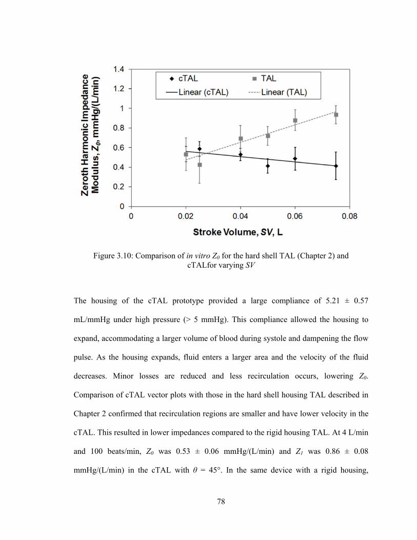
78

The housing of the cTAL prototype provided a large compliance of 5.21 ± 0.57

mL/mmHg under high pressure (> 5 mmHg). This compliance allowed the housing to

expand, accommodating a larger volume of blood during systole and dampening the flow

pulse. As the housing expands, fluid enters a larger area and the velocity of the fluid

decreases. Minor losses are reduced and less recirculation occurs, lowering Z0.

Comparison of cTAL vector plots with those in the hard shell housing TAL described in

Chapter 2 confirmed that recirculation regions are smaller and have lower velocity in the

cTAL. This resulted in lower impedances compared to the rigid housing TAL. At 4 L/min

and 100 beats/min, Z0 was 0.53 ± 0.06 mmHg/(L/min) and Z1 was 0.86 ± 0.08

mmHg/(L/min) in the cTAL with θ = 45°. In the same device with a rigid housing,

Figure 3.10: Comparison of in vitro Z0 for the hard shell TAL (Chapter 2) and cTALfor varying SV

79

Z0=0.69 and Z1=1.22 mmHg/(L/min) [5]. Moreover, unlike TALs with rigid housings, Z0

decreased slightly with increasing SV in the cTAL (Figure 3.10). At SV=0.075, Z0 for the

cTAL and TAL were 0.41 ± 0.14 and 0.94 ± 0.09 mmHg/(L/min), respectively. Thus, at

higher flow rates, such as those experienced during exercise, there is a larger advantage

to using the cTAL.

The lower impedance of the cTAL has implications for use in vivo in both PA-PA

and PA-LA attachment modes. PA-LA attachment would be advantageous in patients

with pulmonary hypertension. Since the device has an impedance much lower than the

natural lungs, blood would flow preferentially through the cTAL. This would allow

significant unloading of the right ventricle and return PA pressures to normal. One can

predict how much the cTAL would lower PA pressures by using the simple formula:

PPA=CO*R+PLA, where PPA is the PA pressure, CO is cardiac output, R is the resistance,

and PLA is the left atrial pressure. Assuming PVR = 4 mmHg/(L/min), PLA = 6 mmHg, and

a cTAL resistance of 1.4 mmHg/(L/min) for the TAL plus anastomoses (adding 0.87

mmHg/(L/min) for the anastomoses) [6], the resulting system resistance with the cTAL

attached in parallel would be 1.0 mmHg/(L/min). Assuming CO=6 L/min, PPA decreases

from 30 mmHg prior to cTAL attachment to 12 mmHg. If the original PVR is 8

mmHg/(L/min), PPA is reduced from 54 mmHg to 13 mmHg.

If the cTAL were attached in series with the native lungs (PA-PA), it would likely

result in similar PA pressure but a reduction in CO due to additive impedances and the

increased work load of the RV. Relationships developed by Kim et al, Kuo et al, and

Akay et al predict the percentage decrease in CO as a result of increases in Z0 and Z1

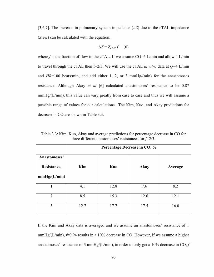
80

[3,6,7]. The increase in pulmonary system impedance (ΔZ) due to the cTAL impedance

(ZcTAL) can be calculated with the equation:

ΔZ = ZcTAL f (6)

where f is the fraction of flow to the cTAL. If we assume CO=6 L/min and allow 4 L/min

to travel through the cTAL then f=2/3. We will use the cTAL in vitro data at Q=4 L/min

and HR=100 beats/min, and add either 1, 2, or 3 mmHg/(min) for the anastomoses

resistance. Although Akay et al [6] calculated anastomoses’ resistance to be 0.87

mmHg/(L/min), this value can vary greatly from case to case and thus we will assume a

possible range of values for our calculations.. The Kim, Kuo, and Akay predictions for

decrease in CO are shown in Table 3.3.

Table 3.3: Kim, Kuo, Akay and average predictions for percentage decrease in CO for three different anastomoses’ resistances for f=2/3.

Percentage Decrease in CO, %

Anastomoses’

Resistance,

mmHg/(L/min)

Kim Kuo Akay Average

1 4.1 12.8 7.6 8.2

2 8.5 15.3 12.6 12.1

3 12.7 17.7 17.5 16.0

If the Kim and Akay data is averaged and we assume an anastomoses’ resistance of 1

mmHg/(L/min), f=0.94 results in a 10% decrease in CO. However, if we assume a higher

anastomoses’ resistance of 3 mmHg/(L/min), in order to only get a 10% decrease in CO, f

81

must be ≤ 0.46. Overall, these predictions are lower than previous devices and may allow

for cTAL attachment in series in a small group of patients without significant pulmonary

hypertension.

Gas transfer in the cTAL is excellent with outlet PO2 and SO2 values above 240

mmHg and 99.5%, respectively, at each tested flow rate. Thus, the cTAL exceeds its gas

transfer goals and the fiber bundle size could be reduced in the future. This could result in

a smaller device, offering the advantage of a smaller prime volume and a lighter, more

“wearable” device. A shortened device would also help to eliminate any low flow or

stasis regions near the distal end.

In conclusion, this cTAL features excellent gas transfer and far lower impedance

than any previous TAL. Its performance in vivo will be described in the following two

chapters. PA-LA and PA-PA in vivo testing will examine the cTAL’s interaction with the

right ventricle as well as its biocompatibility.

82

References

1. Cook KE, Perlman CE, Seipelt R, et al. Hemodynamic and gas transfer properties

of a compliant thoracic artificial lung. ASAIO J 51: 404-411, 2005.

2. Association for the Advance of Medical Instrumentation. Cardiovascular Implants

and Artificial Organs. Blood Gas Exchangers. Arlington, VA: Association for

the Advance of Medical Instrumentation, 1996.

3. Kuo AS, Sato H, Cook KE. Effect of Pulmonary System Impedance on Cardiac

Output. ASAIO Journal 53(2): 53A, 2007.

4. McGillicuddy JW, Chambers SD, Galligan DT, Hirschl RB, Bartlett RH, Cook

KE. In vitro, fluid mechanical effects of thoracic artificial lung compliance.

ASAIO J 51:789-794, 2005.

5. Schewe RE, Khanafer KM, Orizondo RA, Cook KE. Thoracic artificial lung

impedance studies using computational fluid dynamics and in vitro models. Ann

Biomed Eng, Oct. 19, 2011, Epub ahead of print.

6. Akay B, Foucher JA, Camboni D, Koch KL, Kawatra A, Cook KE.

Hemodynamic design requirements for in series thoracic artificial lung attachment

in a model of pulmonary hypertension. ASAIO Journal, Epub ahead of print.

7. Kim J, Sato H, Griffith GW, Cook KE. Cardiac output during high afterload

artificial lung attachment. ASAIO J 55: 73-77, 2009.

83

Chapter 4

In-Parallel cTAL Attachment

Introduction

The most commonly proposed TAL attachment modes are in parallel or in series

with the natural lungs. During in parallel attachment blood flow is routed from the

pulmonary artery (PA), through the TAL and then returned to the left atrium (LA). In

patients with pulmonary hypertension this attachment mode is ideal, as it reduces Z0 for

the combined TAL and natural lung system and thus unloads the right ventricle. In this

setting, TAL attachment should ideally result in a pulmonary system Z0 that is as close as

possible to the healthy natural lung. To accomplish this, the combined resistance of the

TAL and the anastomoses used to attach it must also be close to that of the healthy

natural lung.

The cTAL described in previous chapters was designed to meet this goal. This

study examined pulmonary hemodynamics and cTAL function during in parallel

attachment in healthy sheep. Device flows of 60-90% of CO through the cTAL were

tested both at rest and during simulated exercise.

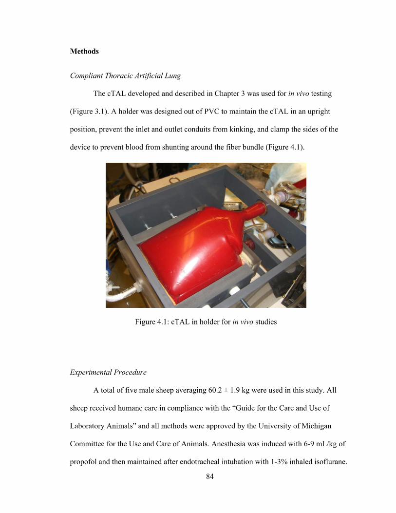
84

Methods

Compliant Thoracic Artificial Lung

The cTAL developed and described in Chapter 3 was used for in vivo testing

(Figure 3.1). A holder was designed out of PVC to maintain the cTAL in an upright

position, prevent the inlet and outlet conduits from kinking, and clamp the sides of the

device to prevent blood from shunting around the fiber bundle (Figure 4.1).

Experimental Procedure

A total of five male sheep averaging 60.2 ± 1.9 kg were used in this study. All

sheep received humane care in compliance with the “Guide for the Care and Use of

Laboratory Animals” and all methods were approved by the University of Michigan

Committee for the Use and Care of Animals. Anesthesia was induced with 6-9 mL/kg of

propofol and then maintained after endotracheal intubation with 1-3% inhaled isoflurane.

Figure 4.1: cTAL in holder for in vivo studies

85

Sheep were mechanical ventilated with oxygen using a Narkomed 6000 ventilator (North

American Dräger, Telford, PA). The ventilator was set to a tidal volume of 10 mL/kg and

a frequency of 12 breaths/min and was adjusted to maintain an arterial partial pressure of

carbon dioxide (PaCO2) between 35 and 45 mmHg. A carotid arterial line and left

jugular venous line were placed and then connected to fluid coupled pressure transducers

(Hospira, Inc., Lake Forest, IL) for the continuous monitoring of arterial and central

venous pressures (PArt and PCV).

A muscle sparing left thoracotomy was performed and the pulmonary artery and

left atrium (LA) were identified. Dacron vascular grafts (Terumo, Ann Arbor, MI) for

artificial lung attachment were attached to the PA and LA. An ultrasonic perivascular

flow probe (Transonic 24AX, Transonic Systems, Inc., Ithaca, NY) was placed around

the PA, proximal to the device inlet graft. This probe was connected to a flow meter

(T400, Transonic Systems, Ithaca, NY) to allow for the measurement of PA flow (QPA).

A pressure catheter (Becton Dickinson and Co., Franklin Lakes, NJ) was then inserted at

the proximal PA and connected to a transducer for the display and recording of the PA

pressure (PPA). A Rommel tourniquet was placed around the distal PA to allow for the

adjustment of flow through the cTAL. Prior to device attachment, 1g of

methylprednisolone (Solu-Medrol, Pfizer, New York, NY) was administered and the

animal was anticoagulated with 100 IU/kg of intravenous sodium heparin (Baxter

Healthcare Corp., Deefield, IL) to maintain active clotting times of above 300 seconds.

The cTAL was primed with heparanized saline (10 U/mL) and then connected to

the PA (device inlet) and LA (device outlet) grafts (Figure 4.2).

86

An ultrasonic flow probe (Transonic 14PXL, Transonic Systems, Inc., Ithaca, NY) was

placed around the inflow conduit and connected to a flow meter (T400, Transonic

Systems Inc., Ithaca, NY) in order to measure device flow (QcTAL). Pressure transducers

were connected to the device inlet and outlet to acquire device inlet and outlet pressure

(Pin and Pout). A suction line was attached to the cTAL gas outlet and 95:5% O2:CO2 with

2-3% vaporized isoflurane between 3 and 9 L/min was used as the sweep gas through the

gas inlet. Sweep gas flow was adjusted during cTAL use to maintain PaCO2 between 35

and 45 mmHg. A Hoffmann clamp was placed around the cTAL outlet conduit to restrict

flow through the device. After cTAL attachment, clamps on the cTAL inlet and outlet

conduits were removed and the Hoffmann clamp was slowly loosened until QcTAL= 1

L/min was achieved. This flow was maintained for 10 minutes for equilibration of fluid

volumes and any inflammatory response. After device attachment, CVP decreased related

Figure 4.2: PA-LA cTAL attachment and instrumentation

87

to the systemic inflammatory response and 500 mL of hetastarch and 500 – 1000 mL of

crystalloid were administered to restore CVP back to baseline values. Thereafter, the

device conduits were clamped off and baseline data was taken, marking the start of the

experiment.

A hemodynamic data set of QPA, QcTAL, Part, PCV, PPA, Pin, Pout were digitally

acquired for 10 seconds at a sampling frequency of 250 Hz through a BIOPAC data

acquisition system (BIOPAC, Goleta, CA). Before attaching the cTAL, an animal

baseline data set was acquired. Rest and exercise conditions were simulated using a

continuous dobutamine (Hospira Inc., Lake Forest, IL) infusion of 0 and then 5

mcg/kg/min, respectively. At each dose, the hemodynamic data set was acquired at

baseline (QcTAL = 0 L/min) and conditions of 60, 75, and 90% of CO shunted to the cTAL

(100*QcTAL/QPA), created by tightening the Rommel tourniquet around the PA. At each

condition, 10 minutes were allowed for equilibration before data was taken. Also, at each

condition, a device exit gas sample was taken along with blood samples from the animal,

device inlet and device outlet.

Data Analysis

The zeroth harmonic pulmonary input impedance modulus, Z0, was calculated at

each flow condition:

0

00 Q

PZ (1)

where P0 is the mean PA pressure and Q0 is the mean PA blood flow rate.

Device resistance, R, was calculated using the formula:

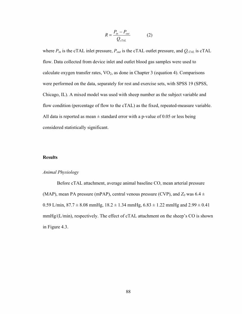
88

cTAL

outin

Q

PPR

(2)

where Pin is the cTAL inlet pressure, Pout is the cTAL outlet pressure, and QcTAL is cTAL

flow. Data collected from device inlet and outlet blood gas samples were used to

calculate oxygen transfer rates, VO2, as done in Chapter 3 (equation 4). Comparisons

were performed on the data, separately for rest and exercise sets, with SPSS 19 (SPSS,

Chicago, IL). A mixed model was used with sheep number as the subject variable and

flow condition (percentage of flow to the cTAL) as the fixed, repeated-measure variable.

All data is reported as mean ± standard error with a p-value of 0.05 or less being

considered statistically significant.

Results

Animal Physiology

Before cTAL attachment, average animal baseline CO, mean arterial pressure

(MAP), mean PA pressure (mPAP), central venous pressure (CVP), and Z0 was 6.4 ±

0.59 L/min, 87.7 ± 8.08 mmHg, 18.2 ± 1.34 mmHg, 6.83 ± 1.22 mmHg and 2.99 ± 0.41

mmHg/(L/min), respectively. The effect of cTAL attachment on the sheep’s CO is shown

in Figure 4.3.

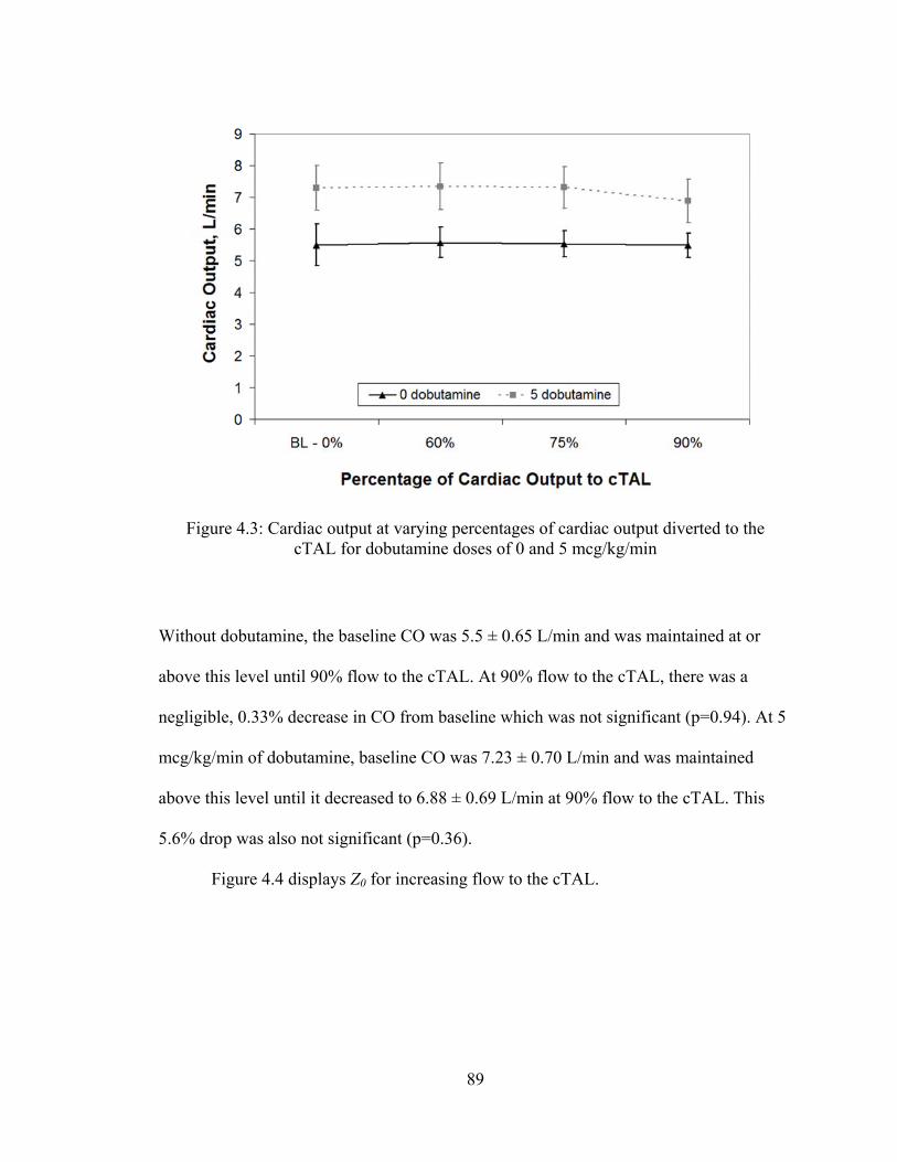
89

Without dobutamine, the baseline CO was 5.5 ± 0.65 L/min and was maintained at or

above this level until 90% flow to the cTAL. At 90% flow to the cTAL, there was a

negligible, 0.33% decrease in CO from baseline which was not significant (p=0.94). At 5

mcg/kg/min of dobutamine, baseline CO was 7.23 ± 0.70 L/min and was maintained

above this level until it decreased to 6.88 ± 0.69 L/min at 90% flow to the cTAL. This

5.6% drop was also not significant (p=0.36).

Figure 4.4 displays Z0 for increasing flow to the cTAL.

Figure 4.3: Cardiac output at varying percentages of cardiac output diverted to the cTAL for dobutamine doses of 0 and 5 mcg/kg/min

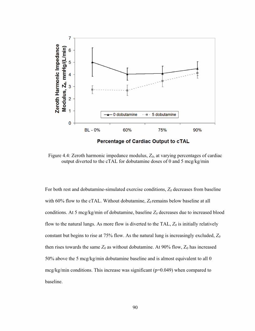
90

For both rest and dobutamine-simulated exercise conditions, Z0 decreases from baseline

with 60% flow to the cTAL. Without dobutamine, Z0 remains below baseline at all

conditions. At 5 mcg/kg/min of dobutamine, baseline Z0 decreases due to increased blood

flow to the natural lungs. As more flow is diverted to the TAL, Z0 is initially relatively

constant but begins to rise at 75% flow. As the natural lung is increasingly excluded, Z0

then rises towards the same Z0 as without dobutamine. At 90% flow, Z0 has increased

50% above the 5 mcg/kg/min dobutamine baseline and is almost equivalent to all 0

mcg/kg/min conditions. This increase was significant (p=0.049) when compared to

baseline.

Figure 4.4: Zeroth harmonic impedance modulus, Z0, at varying percentages of cardiac output diverted to the cTAL for dobutamine doses of 0 and 5 mcg/kg/min

91

MAP and mPAP for both dobutamine levels are displayed in Table 4.1 at each

target and actual percent flow to the cTAL.

Table 4.1: Mean pulmonary artery pressure and mean arterial pressure for varied percentages of the cardiac output to the cTAL

Percentage of CO to cTAL

Dobutamine

Dose Goal Actual

mPAP

(mmHg)

MAP

(mmHg)

0 mcg/kg/min

BL – 0% 0 ± 0% 25.1 ± 5.3 78.4 ± 12.6

60% 62 ± 1% 21.6 ± 4.2 72.3 ± 6.6

75% 74 ± 2% 22.0 ± 4.6 73.5 ± 7.8

90% 91 ± 2% 24.3 ± 5.2 73.1 ± 7.8

5 mcg/kg/min

BL – 0% 0 ± 0% 20.5 ± 1.5 78.5 ± 5.0

60% 61 ± 2% 20.5 ± 2.6 73.2 ± 2.6

75% 76 ± 2% 26.5 ± 3.2 73.7 ± 6.1

90% 93 ± 2% 29.4 ± 3.6 67.3 ± 6.9

BL = baseline; CO = cardiac output; cTAL = compliant thoracic artificial lung; MAP =

mean arterial pressure; mPAP = mean pulmonary artery pressure

The mean baseline PA pressure at 0 mcg/kg/min dobutamine was 25.1 ± 5.31 mmHg

with no significant change at 60, 75 and 90% flow to the cTAL (p = 0.35, 0.46, and 0.86).

At 5 mcg/kg/min dobutamine, mPAP increased from 20.5 ± 1.48 mmHg at baseline to

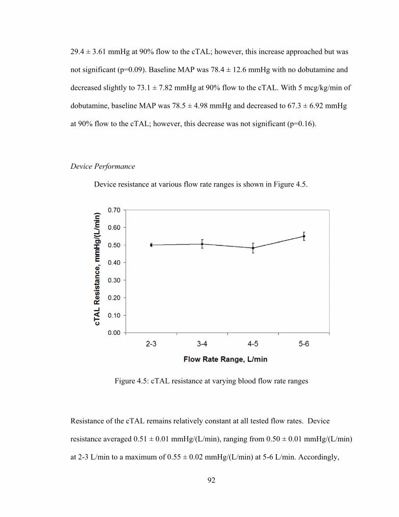
92

29.4 ± 3.61 mmHg at 90% flow to the cTAL; however, this increase approached but was

not significant (p=0.09). Baseline MAP was 78.4 ± 12.6 mmHg with no dobutamine and

decreased slightly to 73.1 ± 7.82 mmHg at 90% flow to the cTAL. With 5 mcg/kg/min of

dobutamine, baseline MAP was 78.5 ± 4.98 mmHg and decreased to 67.3 ± 6.92 mmHg

at 90% flow to the cTAL; however, this decrease was not significant (p=0.16).

Device Performance

Device resistance at various flow rate ranges is shown in Figure 4.5.

Resistance of the cTAL remains relatively constant at all tested flow rates. Device

resistance averaged 0.51 ± 0.01 mmHg/(L/min), ranging from 0.50 ± 0.01 mmHg/(L/min)

at 2-3 L/min to a maximum of 0.55 ± 0.02 mmHg/(L/min) at 5-6 L/min. Accordingly,

Figure 4.5: cTAL resistance at varying blood flow rate ranges

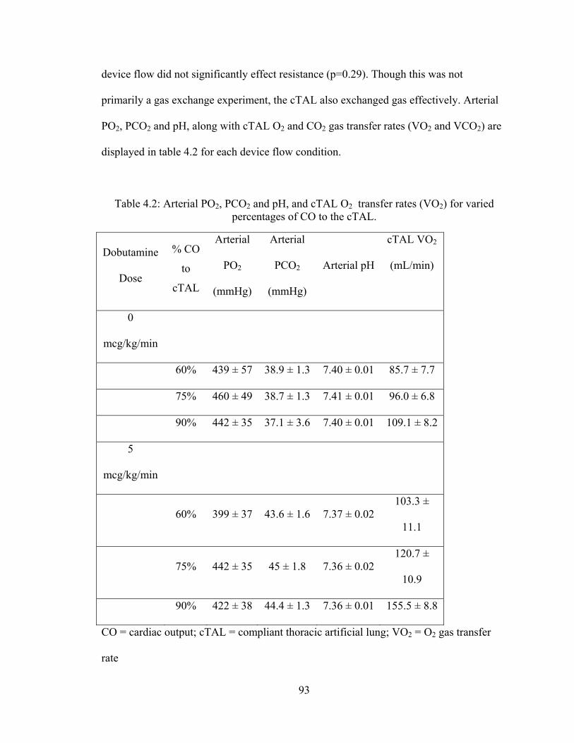
93

device flow did not significantly effect resistance (p=0.29). Though this was not

primarily a gas exchange experiment, the cTAL also exchanged gas effectively. Arterial

PO2, PCO2 and pH, along with cTAL O2 and CO2 gas transfer rates (VO2 and VCO2) are

displayed in table 4.2 for each device flow condition.

Table 4.2: Arterial PO2, PCO2 and pH, and cTAL O2 transfer rates (VO2) for varied percentages of CO to the cTAL.

Dobutamine

Dose

% CO

to

cTAL

Arterial

PO2

(mmHg)

Arterial

PCO2

(mmHg)

Arterial pH

cTAL VO2

(mL/min)

0

mcg/kg/min

60% 439 ± 57 38.9 ± 1.3 7.40 ± 0.01 85.7 ± 7.7

75% 460 ± 49 38.7 ± 1.3 7.41 ± 0.01 96.0 ± 6.8

90% 442 ± 35 37.1 ± 3.6 7.40 ± 0.01 109.1 ± 8.2

5

mcg/kg/min

60% 399 ± 37 43.6 ± 1.6 7.37 ± 0.02 103.3 ±

11.1

75% 442 ± 35 45 ± 1.8 7.36 ± 0.02 120.7 ±

10.9

90% 422 ± 38 44.4 ± 1.3 7.36 ± 0.01 155.5 ± 8.8

CO = cardiac output; cTAL = compliant thoracic artificial lung; VO2 = O2 gas transfer

rate

94

The device outlet oxyhemoglobin saturations were above 99% at every flow condition,

although venous conditions were not sufficient to challenge the device. A typical

hemoglobin and device inlet PO2 was 7.5 and 80 mmHg, respectively. Even with this

higher inlet PO2, VO2 rates ranged from 85.7 ± 7.7 mL/min at 0 dobutamine and 60% CO

to the cTAL to 155.5 ± 8.8 mL/min at 5 dobutamine and 90% CO to the cTAL. Lastly, at

the conclusion of the experiment, there was no visible clot formation in the device.

Discussion

To date, there is no commercially available TAL. Over 18 years of development,

these devices have always featured excellent gas exchange and research has thus focused

on developing devices with progressively lower blood flow resistance and improved

hemodynamics during in vivo attachment [Cook, Cook, Sato]. Ideally, TALs should be

able to provide the majority of the gas exchange while being able to maintain normal

pulmonary hemodynamics.

As there is no commercial device for this application, a few groups have

investigated clinical PA-LA attachment in cases of severe pulmonary hypertension using

the lowest resistance gas exchanger on the market, the Novalung ILA. Two of these

patients had primary pulmonary hypertension and four had pulmonary veno-occlusive

disease. Five of the patients (87%) were successfully bridged [Schmid, Camboni,

Strueber]. Despite this success, the Novalung was not designed for this application. Its

intended use is arterio-venous CO2 removal, which features much lower blood flows of 2

L/min and higher driving pressures. As a result, the Novalung’s gas exchange capabilities

95

are low for the application and the resistance is approximately 5-6 mmHg/(L/min) at

blood flows of 2-2.5 L/min [Florchinger, Muller, Wiebe]. To support COPD, IPF, and

septic patients, greater gas exchange will be required. Moreover, in cases of marked

pulmonary hypertension, it would be ideal to be able to fully unload the RV and eliminate

the need for inotropes.

In the current study, the new cTAL design was tested in healthy animals with

normal PA pressure. Therefore, the goal for this study was to maintain normal PA

pressures and CO with up to 90% of CO diverted to the cTAL. Results indicate that these

goals were met. cTAL attachment caused only minimal, statistically insignificant

decreases in CO and increases in PA pressure from baseline at all conditions. At the most

extreme condition, simulated exercise with 90% of the CO diverted to the cTAL, CO

decreased 5.6% and PA pressure increased 8.8 mmHg. This, however, represents an

extreme case. A more typical, and advisable [Takewa], condition would likely be 75% of

CO. Here, CO was identical to baseline values, and PA pressure decreased at rest and

increased a small amount during simulated exercise.

Maintenance of normal pulmonary hemodynamics was the result of very low

cTAL resistance. Average resistance for the range of flows tested was 0.51 ± 0.01

mmHg/(L/min), well below that of the natural lung. Moreover, the resistance of the

device did not change significantly as flow increased. The low cTAL resistance, in turn,

maintains low Z0. Previous studies have shown that Z0 is the dominant variable affecting

CO during TAL attachment, with CO decreasing as Z0 increases [Kim, Kuo, Akay]. In

this study, Z0 is lower than baseline at 60% flow to the cTAL due to the second, parallel

flow path provided by the cTAL and the minimal banding of the PA at that condition. As

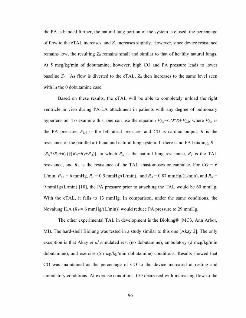
96

the PA is banded further, the natural lung portion of the system is closed, the percentage

of flow to the cTAL increases, and Z0 increases slightly. However, since device resistance

remains low, the resulting Z0 remains small and similar to that of healthy natural lungs.

At 5 mcg/kg/min of dobutamine, however, high CO and PA pressure leads to lower

baseline Z0. As flow is diverted to the cTAL, Z0 then increases to the same level seen

with in the 0 dobutamine case.

Based on these results, the cTAL will be able to completely unload the right

ventricle in vivo during PA-LA attachment in patients with any degree of pulmonary

hypertension. To examine this, one can use the equation PPA=CO*R+PLA, where PPA is

the PA pressure, PLA is the left atrial pressure, and CO is cardiac output. R is the

resistance of the parallel artificial and natural lung system. If there is no PA banding, R =

[RN*(RT+RA)]/[RN+RT+RA)], in which RN is the natural lung resistance, RT is the TAL

resistance, and RA is the resistance of the TAL anastomoses or cannulae. For CO = 6

L/min, PLA = 6 mmHg, RT = 0.5 mmHg/(L/min), and RA = 0.87 mmHg/(L/min), and RN =

9 mmHg/(L/min) [10], the PA pressure prior to attaching the TAL would be 60 mmHg.

With the cTAL, it falls to 13 mmHg. In comparison, under the same conditions, the

Novalung ILA (RT = 6 mmHg/(L/min)) would reduce PA pressure to 29 mmHg.

The other experimental TAL in development is the Biolung® (MC3, Ann Arbor,

MI). The hard-shell Biolung was tested in a study similar to this one [Akay 2]. The only

exception is that Akay et al simulated rest (no dobutamine), ambulatory (2 mcg/kg/min

dobutamine), and exercise (5 mcg/kg/min dobutamine) conditions. Results showed that

CO was maintained as the percentage of CO to the device increased at resting and

ambulatory conditions. At exercise conditions, CO decreased with increasing flow to the

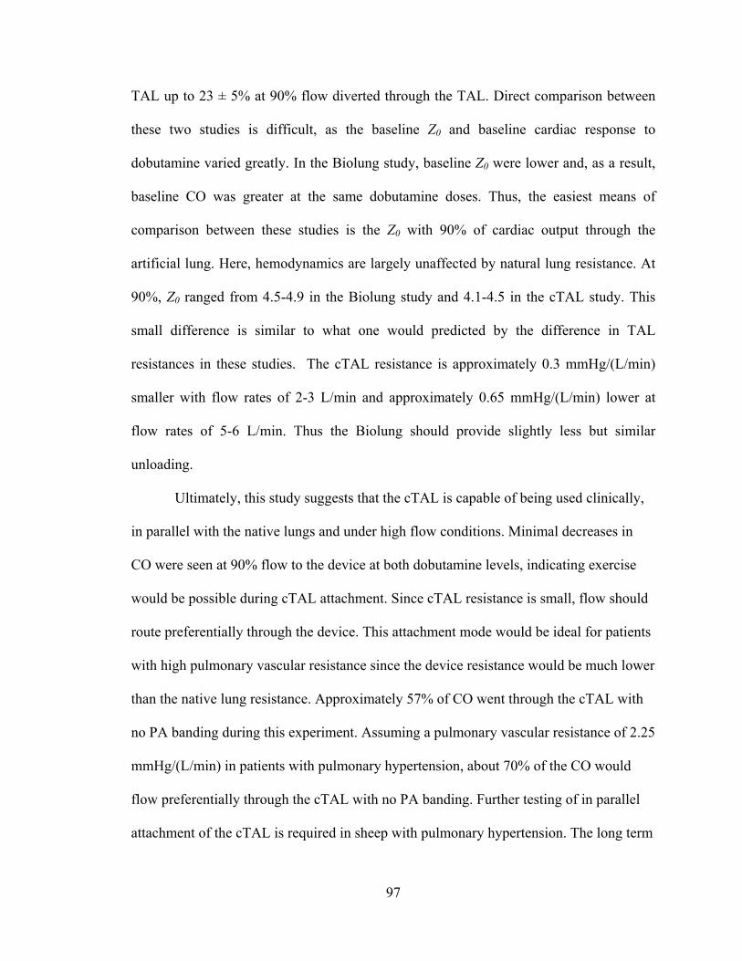
97

TAL up to 23 ± 5% at 90% flow diverted through the TAL. Direct comparison between

these two studies is difficult, as the baseline Z0 and baseline cardiac response to

dobutamine varied greatly. In the Biolung study, baseline Z0 were lower and, as a result,

baseline CO was greater at the same dobutamine doses. Thus, the easiest means of

comparison between these studies is the Z0 with 90% of cardiac output through the

artificial lung. Here, hemodynamics are largely unaffected by natural lung resistance. At

90%, Z0 ranged from 4.5-4.9 in the Biolung study and 4.1-4.5 in the cTAL study. This

small difference is similar to what one would predicted by the difference in TAL

resistances in these studies. The cTAL resistance is approximately 0.3 mmHg/(L/min)

smaller with flow rates of 2-3 L/min and approximately 0.65 mmHg/(L/min) lower at

flow rates of 5-6 L/min. Thus the Biolung should provide slightly less but similar

unloading.

Ultimately, this study suggests that the cTAL is capable of being used clinically,

in parallel with the native lungs and under high flow conditions. Minimal decreases in

CO were seen at 90% flow to the device at both dobutamine levels, indicating exercise

would be possible during cTAL attachment. Since cTAL resistance is small, flow should

route preferentially through the device. This attachment mode would be ideal for patients

with high pulmonary vascular resistance since the device resistance would be much lower

than the native lung resistance. Approximately 57% of CO went through the cTAL with

no PA banding during this experiment. Assuming a pulmonary vascular resistance of 2.25

mmHg/(L/min) in patients with pulmonary hypertension, about 70% of the CO would

flow preferentially through the cTAL with no PA banding. Further testing of in parallel

attachment of the cTAL is required in sheep with pulmonary hypertension. The long term

98

effects of in parallel cTAL attachment will also be studied for up to 30 days in healthy

sheep and sheep with pulmonary hypertension.

Conclusion

The cTAL resistance is lower than the natural lung, averaging 0.51 ± 0.03

mmHg/(L/min). Use of the cTAL in a PA-LA configuration caused no change in CO

under rest and exercise conditions. Thus, the cTAL can provide PA-LA respiratory

support without significant changes in pulmonary hemodynamics in healthy sheep and

will be capable of unloading the RV in subjects with pulmonary hypertension.

99

References

1. Cook KE: Design and Testing of Intrathoracic Artificial Lungs. PhD Thesis.

Northwestern University, 1996.

2. Cook KE, Perlman CE, Seipelt R, et al: Hemodynamic and Gas Transfer

Properties of a Compliant Thoracic Artificial Lung. ASAIO J 51: 404-411, 2005.

3. Sato H, McGillicuddy JH, Griffith GW, et al: Effect of Artificial Lung

Compliance on In Vivo Pulmonary System Hemodynamics. ASAIO J 52: 248-256,

2006.

4. Schmid C, Philipp A, Hilker M, et al. Bridge to Lung Transplantation Through a

Pulmonary Artery to Left Atrial Oxygenator Circuit. Ann Thorac Surg 85:1202-5,

2008.

5. Camboni D, Philipp A, Arlt M, et al. First Experience With a Paracorporeal

Artificial Lung in Humans. ASAIO J 55:304-307, 2009.

6. Strueber M, Hoeper MM, Fischer S, et al. Bridge to Thoracic Organ

Transplantation in Patients with Pulmonary Arterial Hypertension Using a

Pumpless Lung Assist Device. American Journal of Transplantation 9:853-857,

2009.

7. Flörchinger B, Philipp A, Klose A, Hilker M, Kobuch R, Rupprecht L, Keyser A,

Pühler T, Hirt S, Wiebe K, Müller T, Langgartner J, Lehle K, Schmid C.

Pumpless extracorporeal lung assist: a 10-year institutional experience. Ann

Thorac Surg 86:410-7, 2008.

8. Müller T, Lubnow M, Philipp A, Bein T, Jeron A, Luchner A, Rupprecht L, Reng

M, Langgartner J, Wrede CE, Zimmermann M, Birnbaum D, Schmid C, Riegger

100

GA, Pfeifer M. Extracorporeal pumpless interventional lung assist in clinical

practice: determinants of efficacy. Eur Respir J 33:551-8, 2009.

9. Wiebe K, Poeling J, Arlt M, Philipp A, Camboni D, Hofmann S, Schmid C.

Thoracic surgical procedures supported by a pumpless interventional lung assist.

Ann Thorac Surg 89:1782-7, 2010.

10. Takewa Y, Tatsumi E, Taenaka Y, Eya K, et al. Hemodynamic and humoral

conditions in stepwise reduction of pulmonary blood flow during venoarterial

bypass in awake goats. ASAIO J 43(5): M494-9, 1997.

11. Kim J, Sato H, Griffith GW, Cook KE. Cardiac output during high afterload

artificial lung attachment. ASAIO J 55: 73-77, 2009.

12. Kuo AS, Sato H, Reoma JL, Cook KE. The relationship between pulmonary

system impedance and right ventricular function in normal sheep. Cardiovascular

Engineering 9: 153-160, 2009.

13. Akay B, Foucher JA, Camboni D, Koch KL, Kawatra A, Cook KE.

Hemodynamic design requirements for in series thoracic artificial lung attachment

in a model of pulmonary hypertension. ASAIO Journal, submitted.

14. Akay B, Reoma JL, Camboni D, et al. In-parallel artificial lung attachment at

high flows in normal and pulmonary hypertension models. Ann Thorac Surg 90:

259-65, 2010.

101

Chapter 5

In-Series cTAL Attachment

Introduction

While the cTAL had excellent in vivo performance in parallel, there is the

constant risk of life-threatening air emboli and thromboemboli in this attachment mode.

An alternative configuration is in series attachment with the natural lungs. In this mode,

blood is routed from the proximal pulmonary artery (PA) through the cTAL and then

back to the distal PA where the blood then flows through the native lungs and finally

back to the LA. This configuration eliminates the risk of systemic emboli by allowing the

lung to perform its filtration and non-respiratory functions. In addition, the entire cardiac

output (CO) can flow through the cTAL, allowing for complete gas exchange. However,

studies on TAL attachment mode have shown series attachment to increase pulmonary

system impedance and decrease CO [1]. Increased pulmonary system impedance is

caused by the additive impedance of the TAL and natural lung. Therefore, it is imperative

that the device have the lowest impedance possible to prevent RV failure when attached

in series.

The low-resistance cTAL developed and tested in previous chapters was

examined in this setting. This study examined pulmonary hemodynamics and cTAL

function during in series attachment in healthy sheep. As in the PA-LA study, described

102

in Chapter 4, different device flows were tested with 60-90% of CO through the cTAL

both at rest and during simulated exercise.

Methods

Experimental Procedure

Five male sheep averaging 63 ± 0.92 kg were used in this study. All sheep

received humane care in compliance with the “Guide for the Care and Use of Laboratory

Animals” and all methods were approved by the University of Michigan Committee for

the Use and Care of Animals. Anesthesia was induced with 6-9 mL/kg of propofol and

then maintained after endotracheal intubation with 1-3% inhaled isoflurane (Abbot

Laboratories, Chicago, IL). Sheep were mechanically ventilated with oxygen using a

Narkomed 6000 ventilator (North American Dräger, Telford, PA). The ventilator was set

to a tidal volume of 10 mL/kg and a frequency of 12 breaths/min and was adjusted to

maintain an arterial PCO2 (PaCO2) between 35 and 45 mmHg. A carotid arterial line and

left jugular venous line were placed and then connected to fluid coupled pressure

transducers (ICU Medical, Inc., San Clemente, CA) for the continuous monitoring of

arterial and central venous pressures (PArt and PCV).

A muscle sparing left anterolateral thoracotomy was performed and the fourth rib

was removed. The left lung was packed laterally and the pericardium was incised. The

PA was then identified. Low porosity woven Dacron vascular grafts 18 mm in size

(Boston Scientific, Natick, MA) solvent bonded to 5/8” inner diameter PVC tubing

(Fisher Scientific, Pittsburgh, PA) were used as conduits for artificial lung attachment.

An end-to-side anastomosis was performed between the device outlet conduit and the

103

distal PA near the bifurcation. The device inlet end-to-side anastomosis was then

performed on the proximal PA. An ultrasonic perivascular flow probe (Transonic 24AX,

Transonic Systems, Inc., Ithaca, NY) was placed around the PA, proximal to the device

inlet graft. This probe was connected to a flow meter (T400, Transonic Systems, Ithaca,

NY) to allow for the measurement of PA flow (QPA). A pressure catheter (Becton

Dickinson and Co., Franklin Lakes, NJ) was then inserted at the proximal PA and

connected to a transducer for the display and recording of the proximal PA pressure

(PPAP). A Rommel tourniquet was placed around the PA between the inlet and outlet

grafts to allow for the adjustment of flow through the cTAL. Pressure catheters were

inserted into the distal PA near the bifurcation and into the left atrium to allow for the

recording of the distal PA pressure (PPAD) and the left atrial pressure (PLA), which

facilitated the calculation of the pulmonary vascular resistance (PVR) of the native lungs.

Prior to device attachment, 1g of methylprednisolone (Solu-Medrol, Pfizer, New York,

NY) was administered, and the animal was anticoagulated with 100 IU/kg of intravenous

sodium heparin (Baxter Healthcare Corp., Deerfield, IL) to maintain active clotting times

of above 300 seconds.

The cTAL was primed with heparinized saline (10 U/mL) and then connected to

the proximal PA (device inlet) and distal PA (device outlet) grafts (Figure 5.1).

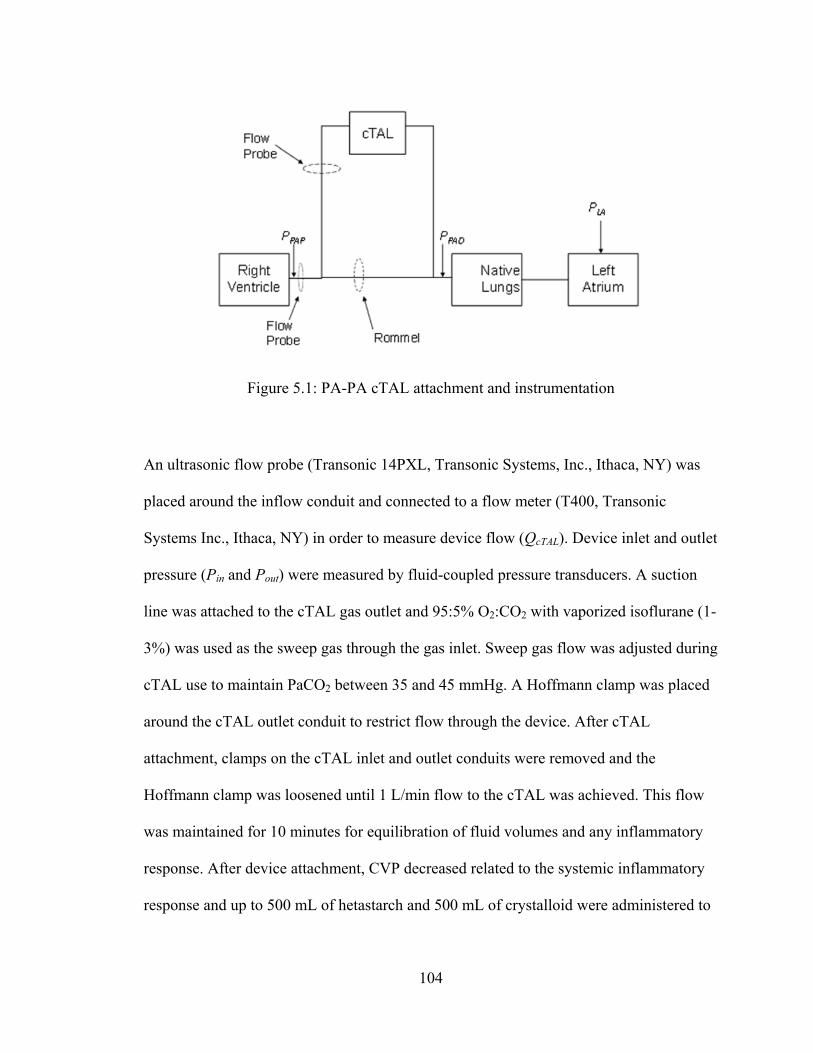
104

An ultrasonic flow probe (Transonic 14PXL, Transonic Systems, Inc., Ithaca, NY) was

placed around the inflow conduit and connected to a flow meter (T400, Transonic

Systems Inc., Ithaca, NY) in order to measure device flow (QcTAL). Device inlet and outlet

pressure (Pin and Pout) were measured by fluid-coupled pressure transducers. A suction

line was attached to the cTAL gas outlet and 95:5% O2:CO2 with vaporized isoflurane (1-

3%) was used as the sweep gas through the gas inlet. Sweep gas flow was adjusted during

cTAL use to maintain PaCO2 between 35 and 45 mmHg. A Hoffmann clamp was placed

around the cTAL outlet conduit to restrict flow through the device. After cTAL

attachment, clamps on the cTAL inlet and outlet conduits were removed and the

Hoffmann clamp was loosened until 1 L/min flow to the cTAL was achieved. This flow

was maintained for 10 minutes for equilibration of fluid volumes and any inflammatory

response. After device attachment, CVP decreased related to the systemic inflammatory

response and up to 500 mL of hetastarch and 500 mL of crystalloid were administered to

Figure 5.1: PA-PA cTAL attachment and instrumentation

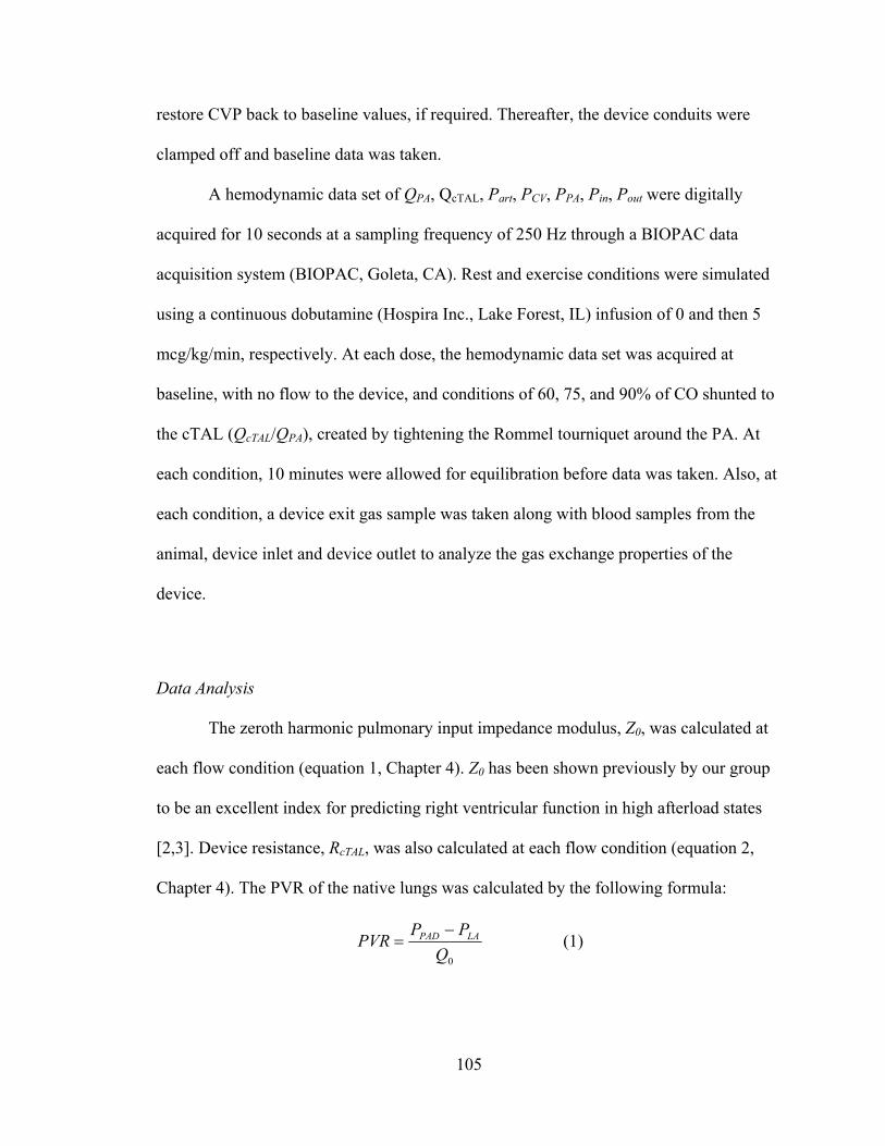
105

restore CVP back to baseline values, if required. Thereafter, the device conduits were

clamped off and baseline data was taken.

A hemodynamic data set of QPA, QcTAL, Part, PCV, PPA, Pin, Pout were digitally

acquired for 10 seconds at a sampling frequency of 250 Hz through a BIOPAC data

acquisition system (BIOPAC, Goleta, CA). Rest and exercise conditions were simulated

using a continuous dobutamine (Hospira Inc., Lake Forest, IL) infusion of 0 and then 5

mcg/kg/min, respectively. At each dose, the hemodynamic data set was acquired at

baseline, with no flow to the device, and conditions of 60, 75, and 90% of CO shunted to

the cTAL (QcTAL/QPA), created by tightening the Rommel tourniquet around the PA. At

each condition, 10 minutes were allowed for equilibration before data was taken. Also, at

each condition, a device exit gas sample was taken along with blood samples from the

animal, device inlet and device outlet to analyze the gas exchange properties of the

device.

Data Analysis

The zeroth harmonic pulmonary input impedance modulus, Z0, was calculated at

each flow condition (equation 1, Chapter 4). Z0 has been shown previously by our group

to be an excellent index for predicting right ventricular function in high afterload states

[2,3]. Device resistance, RcTAL, was also calculated at each flow condition (equation 2,

Chapter 4). The PVR of the native lungs was calculated by the following formula:

0Q

PPPVR LAPAD

(1)

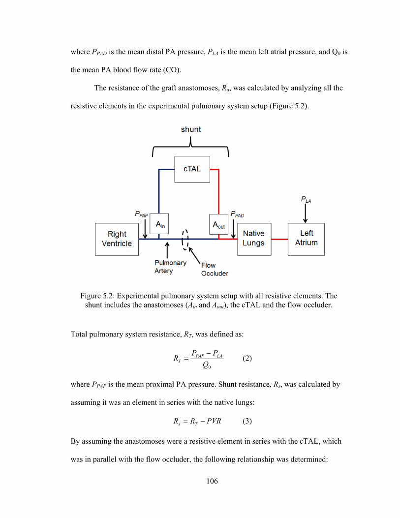
106

where PPAD is the mean distal PA pressure, PLA is the mean left atrial pressure, and Q0 is

the mean PA blood flow rate (CO).

The resistance of the graft anastomoses, Ra, was calculated by analyzing all the

resistive elements in the experimental pulmonary system setup (Figure 5.2).

Total pulmonary system resistance, RT, was defined as:

0Q

PPR LAPAP

T

(2)

where PPAP is the mean proximal PA pressure. Shunt resistance, Rs, was calculated by

assuming it was an element in series with the native lungs:

PVRRR Ts (3)

By assuming the anastomoses were a resistive element in series with the cTAL, which

was in parallel with the flow occluder, the following relationship was determined:

Figure 5.2: Experimental pulmonary system setup with all resistive elements. The shunt includes the anastomoses (Ain and Aout), the cTAL and the flow occluder.

107

FOacTALs RRRR

111

(4)

where RFO is the resistance of the flow occluder defined using a flow relationship:

f

RRfR acTAL

FO

1

)( (5)

where f is the fraction of Q0 diverted to the cTAL. Using equations 4 and 5, an equation

for Ra was determined:

cTALs

a Rf

RR (6)

Ra was calculated at each flow condition and an equation for approximate Ra as a

function of f was determined.

Statistical analysis was performed separately for the 0 and 5 mcg/kg/min data

sets. The analysis of baseline PVR before and after cTAL attachment was conducted

using a paired two-tailed student’s t-test assuming equal variances. All other statistical

comparisons were performed using a mixed model with sheep number as the subject

variable and flow condition as the fixed, repeated-measure variable. The statistical

analysis was performed using SPSS 19 (SPSS, Chicago, IL). All data is reported as the

mean ± the standard error and a p-value of 0.05 or less was considered statistically

significant.

Results

Animal Physiology

Before cTAL attachment, average animal baseline CO, mean arterial pressure

(MAP), mean PA pressure (mPAP), central venous pressure (CVP), PVR, and Z0 was 6.5

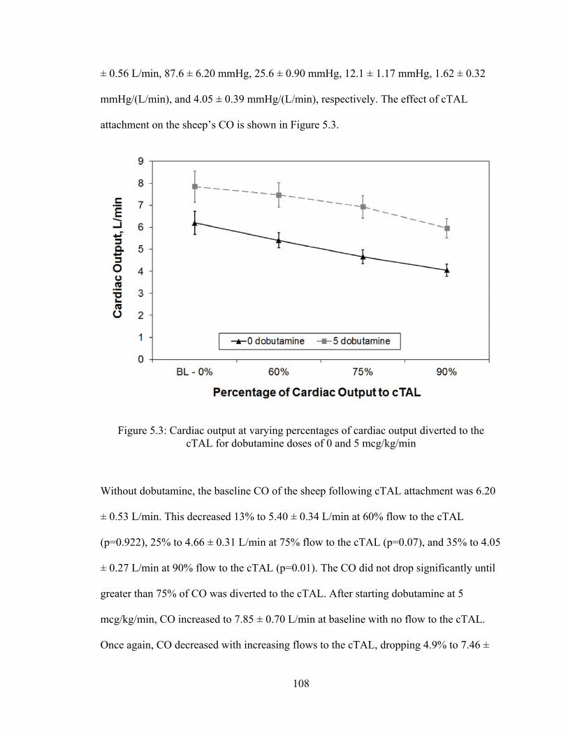
108

± 0.56 L/min, 87.6 ± 6.20 mmHg, 25.6 ± 0.90 mmHg, 12.1 ± 1.17 mmHg, 1.62 ± 0.32

mmHg/(L/min), and 4.05 ± 0.39 mmHg/(L/min), respectively. The effect of cTAL

attachment on the sheep’s CO is shown in Figure 5.3.

Without dobutamine, the baseline CO of the sheep following cTAL attachment was 6.20

± 0.53 L/min. This decreased 13% to 5.40 ± 0.34 L/min at 60% flow to the cTAL

(p=0.922), 25% to 4.66 ± 0.31 L/min at 75% flow to the cTAL (p=0.07), and 35% to 4.05

± 0.27 L/min at 90% flow to the cTAL (p=0.01). The CO did not drop significantly until

greater than 75% of CO was diverted to the cTAL. After starting dobutamine at 5

mcg/kg/min, CO increased to 7.85 ± 0.70 L/min at baseline with no flow to the cTAL.

Once again, CO decreased with increasing flows to the cTAL, dropping 4.9% to 7.46 ±

Figure 5.3: Cardiac output at varying percentages of cardiac output diverted to the cTAL for dobutamine doses of 0 and 5 mcg/kg/min

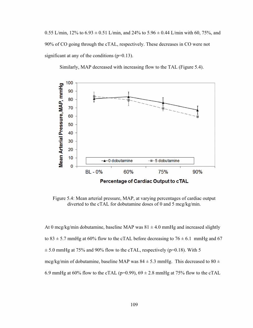
109

0.55 L/min, 12% to 6.93 ± 0.51 L/min, and 24% to 5.96 ± 0.44 L/min with 60, 75%, and

90% of CO going through the cTAL, respectively. These decreases in CO were not

significant at any of the conditions (p=0.13).

Similarly, MAP decreased with increasing flow to the TAL (Figure 5.4).

At 0 mcg/kg/min dobutamine, baseline MAP was 81 ± 4.0 mmHg and increased slightly

to 83 ± 5.7 mmHg at 60% flow to the cTAL before decreasing to 76 ± 6.1 mmHg and 67

± 5.0 mmHg at 75% and 90% flow to the cTAL, respectively (p=0.18). With 5

mcg/kg/min of dobutamine, baseline MAP was 84 ± 5.3 mmHg. This decreased to 80 ±

6.9 mmHg at 60% flow to the cTAL (p=0.99), 69 ± 2.8 mmHg at 75% flow to the cTAL

Figure 5.4: Mean arterial pressure, MAP, at varying percentages of cardiac output diverted to the cTAL for dobutamine doses of 0 and 5 mcg/kg/min.

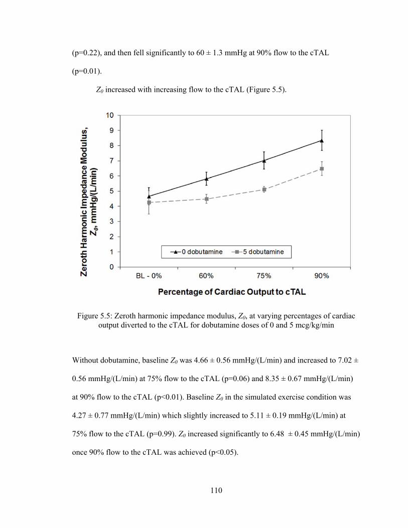
110

(p=0.22), and then fell significantly to 60 ± 1.3 mmHg at 90% flow to the cTAL

(p=0.01).

Z0 increased with increasing flow to the cTAL (Figure 5.5).

Without dobutamine, baseline Z0 was 4.66 ± 0.56 mmHg/(L/min) and increased to 7.02 ±

0.56 mmHg/(L/min) at 75% flow to the cTAL (p=0.06) and 8.35 ± 0.67 mmHg/(L/min)

at 90% flow to the cTAL (p<0.01). Baseline Z0 in the simulated exercise condition was

4.27 ± 0.77 mmHg/(L/min) which slightly increased to 5.11 ± 0.19 mmHg/(L/min) at

75% flow to the cTAL (p=0.99). Z0 increased significantly to 6.48 ± 0.45 mmHg/(L/min)

once 90% flow to the cTAL was achieved (p<0.05).

Figure 5.5: Zeroth harmonic impedance modulus, Z0, at varying percentages of cardiac output diverted to the cTAL for dobutamine doses of 0 and 5 mcg/kg/min

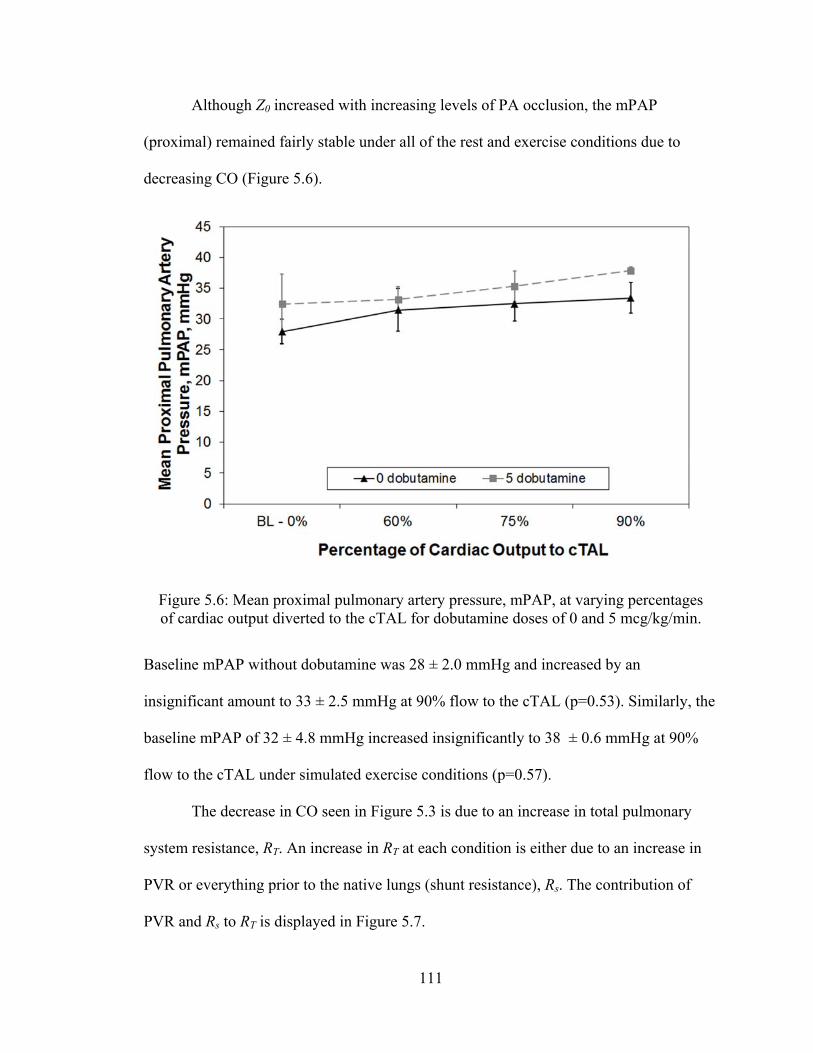
111

Although Z0 increased with increasing levels of PA occlusion, the mPAP

(proximal) remained fairly stable under all of the rest and exercise conditions due to

decreasing CO (Figure 5.6).

Baseline mPAP without dobutamine was 28 ± 2.0 mmHg and increased by an

insignificant amount to 33 ± 2.5 mmHg at 90% flow to the cTAL (p=0.53). Similarly, the

baseline mPAP of 32 ± 4.8 mmHg increased insignificantly to 38 ± 0.6 mmHg at 90%

flow to the cTAL under simulated exercise conditions (p=0.57).

The decrease in CO seen in Figure 5.3 is due to an increase in total pulmonary

system resistance, RT. An increase in RT at each condition is either due to an increase in

PVR or everything prior to the native lungs (shunt resistance), Rs. The contribution of

PVR and Rs to RT is displayed in Figure 5.7.

Figure 5.6: Mean proximal pulmonary artery pressure, mPAP, at varying percentages of cardiac output diverted to the cTAL for dobutamine doses of 0 and 5 mcg/kg/min.

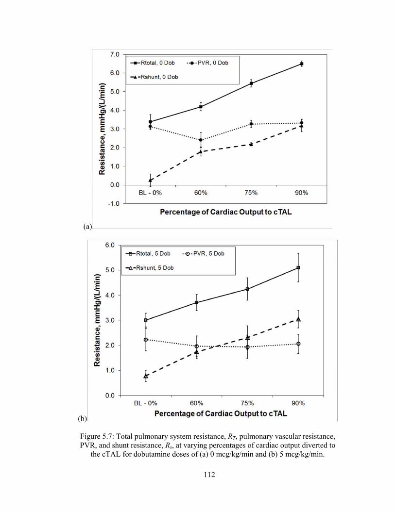
112

(a)

(b)

Figure 5.7: Total pulmonary system resistance, RT, pulmonary vascular resistance, PVR, and shunt resistance, Rs, at varying percentages of cardiac output diverted to

the cTAL for dobutamine doses of (a) 0 mcg/kg/min and (b) 5 mcg/kg/min.

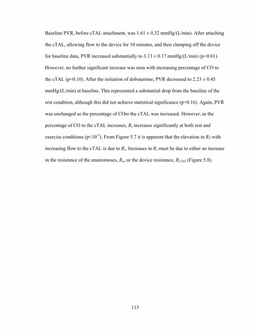
113

Baseline PVR, before cTAL attachment, was 1.61 ± 0.32 mmHg/(L/min). After attaching

the cTAL, allowing flow to the device for 10 minutes, and then clamping off the device

for baseline data, PVR increased substantially to 3.13 ± 0.17 mmHg/(L/min) (p=0.01).

However, no further significant increase was seen with increasing percentage of CO to

the cTAL (p=0.10). After the initiation of dobutamine, PVR decreased to 2.23 ± 0.45

mmHg/(L/min) at baseline. This represented a substantial drop from the baseline of the

rest condition, although this did not achieve statistical significance (p=0.16). Again, PVR

was unchanged as the percentage of COto the cTAL was increased. However, as the

percentage of CO to the cTAL increases, Rs increases significantly at both rest and

exercise conditions (p<10-3). From Figure 5.7 it is apparent that the elevation in RT with

increasing flow to the cTAL is due to Rs. Increases in Rs must be due to either an increase

in the resistance of the anastomoses, Ra, or the device resistance, RcTAL (Figure 5.8).

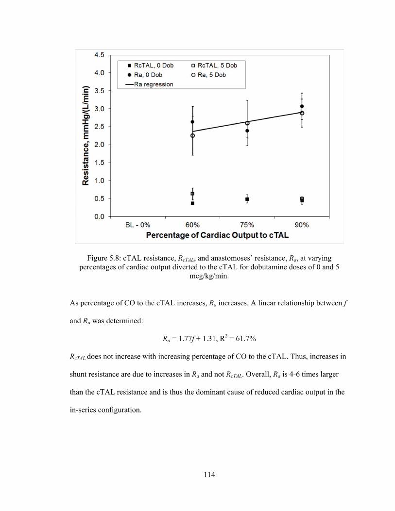
114

As percentage of CO to the cTAL increases, Ra increases. A linear relationship between f

and Ra was determined:

Ra = 1.77f + 1.31, R2 = 61.7%

RcTAL does not increase with increasing percentage of CO to the cTAL. Thus, increases in

shunt resistance are due to increases in Ra and not RcTAL. Overall, Ra is 4-6 times larger

than the cTAL resistance and is thus the dominant cause of reduced cardiac output in the

in-series configuration.

Figure 5.8: cTAL resistance, RcTAL, and anastomoses’ resistance, Ra, at varying percentages of cardiac output diverted to the cTAL for dobutamine doses of 0 and 5

mcg/kg/min.

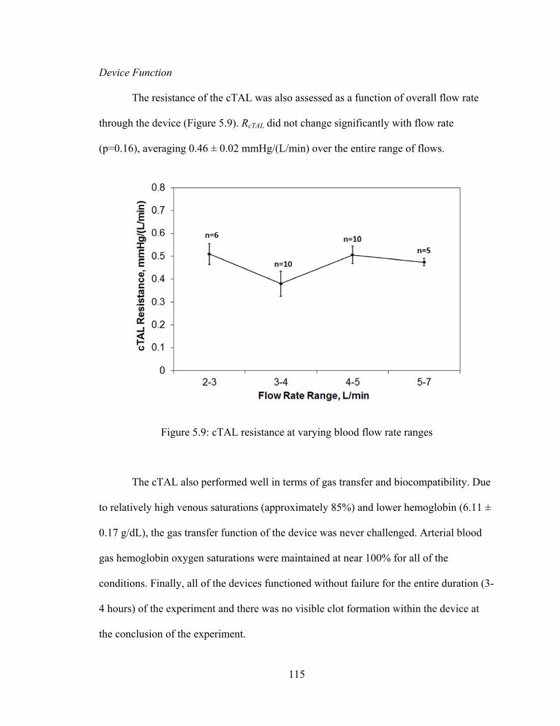
115

Device Function

The resistance of the cTAL was also assessed as a function of overall flow rate

through the device (Figure 5.9). RcTAL did not change significantly with flow rate

(p=0.16), averaging 0.46 ± 0.02 mmHg/(L/min) over the entire range of flows.

The cTAL also performed well in terms of gas transfer and biocompatibility. Due

to relatively high venous saturations (approximately 85%) and lower hemoglobin (6.11 ±

0.17 g/dL), the gas transfer function of the device was never challenged. Arterial blood

gas hemoglobin oxygen saturations were maintained at near 100% for all of the

conditions. Finally, all of the devices functioned without failure for the entire duration (3-

4 hours) of the experiment and there was no visible clot formation within the device at

the conclusion of the experiment.

Figure 5.9: cTAL resistance at varying blood flow rate ranges

116

Discussion

As discovered in Chapter 4, cTAL resistance did not change significantly with

flow. In the current study, average cTAL resistance was 0.46 ± 0.02 mmHg/(L/min),

similar to results from Chapter 4. Though cTAL resistance did not increase with

increasing percentage flow to the device, Z0 did increase. This increase was due to an

increase in the shunt resistance and not PVR. There was an initial 94% increase in PVR

from animal baseline during an initial equilibration phase following attachment of the

cTAL due to an inflammatory response to the device. However, after this initial increase,

the PVR did not increase significantly as percentage flow to the cTAL increased.

Resistance of the shunt did, however, increase with increasing flow. Thus, increases in

pulmonary system resistance with increasing flow diversion to the cTAL were due to

increasing resistance of the anastomoses. These values were higher than predicted

previously [4] but anastomoses’ resistance can vary greatly from case to case.

Theoretically, at baseline (no flow to the cTAL), RT should have equaled PVR; however,

this was not the case. There was a small additional resistance in the system, most likely

from the anastomoses, suggesting the anastomoses cannot be treated as an element

completely in series with the cTAL.

Based on previous predictions and the results in this chapter, we can make

predictions on how much flow through the cTAL could be tolerated by patients. As

discussed in earlier chapters, previous studies concluded that Z0 is the dominant variable

affecting CO during TAL attachment, with CO decreasing as Z0 increases [2-4]. This was

again found to be true in this study. For both dobutamine levels, as the percentage of CO

117

to the cTAL increased, Z0 increased, causing CO to decrease. CO only decreased

significantly at 90% of CO to the cTAL with 0 mcg/kg/min dobutamine. However, at the

other conditions, there were percent decreases in CO that would not be acceptable for

patient use. At 60% flow to the cTAL, with 0 and 5 mcg/kg/min, CO decreased 13% and

5%, respectively. Therefore, cTAL flows above 60% of CO are not advisable during PA-

PA attachment in patients. From their study on the effects of impedance during PA-PA

attachment, Akay et al determined that TAL resistance must be less than 1.81, 0.92, and

0.47 mmHg/(L/min) for 50, 75, and 100% of CO to the TAL to limit the drop in CO to

less than 10%. However, they also calculated resistance of the anastomoses to be 0.87

mmHg/(L/min). In our study, the anastomoses resistance went up with increasing flow to

the device and averaged 2.64 mmHg/(L/min). In Chapter 3, it was predicted that with an

anastomoses’ resistance of 3 mmHg/(L/min), the percentage flow to the cTAL must be

less than 46% for a decrease in CO less than 10%. Using the average cTAL and

anastomoses’ resistance presented in this chapter, the percentage of CO to the cTAL must

be ≤ 53% to maintain CO within 10% of baseline. Therefore, if anastomoses’ resistance

is high, as in this study, the percentage of CO to the cTAL during PA-PA attachment

should be kept around 50%. This warrants further examination in long-term cTAL

studies. Results in these studies may vary due to additional variables, including

anesthesia, animal health, and the length of cTAL attachment.

118

References

1. Perlman CE, Cook KE, Seipelt R, Mavroudis C, Backer CL, Mockros LF. In vivo

hemodynamic responses to artificial lung attachment. ASAIO J 51: 412-425, 2005.

2. Kim J, Sato H, Griffith GW, Cook KE. Cardiac output during high afterload

artificial lung attachment. ASAIO J 55: 73-77, 2009.

3. Kuo AS, Sato H, Reoma JL, Cook KE. The relationship between pulmonary

system impedance and right ventricular function in normal sheep. Cardiovascular

Engineering 9: 153-160, 2009.

4. Akay B, Foucher JA, Camboni D, Koch KL, Kawatra A, Cook KE.

Hemodynamic design requirements for in series thoracic artificial lung attachment

in a model of pulmonary hypertension. ASAIO Journal, submitted.

119

Chapter 6

Conclusion

Conclusions

This work examined the effect of different housing geometries and materials on

TAL impedance and flow uniformity. From CFD and in vitro studies, the optimal TAL

geometry was determined. A cTAL with this design was prototyped for in vitro and in

vivo testing. The in vivo performance of the optimized cTAL was tested in two different

attachment modes under simulated rest and exercise conditions. From these studies, it can

be concluded that:

1. More gradual device entrances and exits result in reductions in TAL impedance.

Recirculation in the inlet housing region is reduced as θ decreases, reducing

overal device impedance. This was also the case for the cTAL, as confirmed by

FSI analysis.

2. A region of little to no flow exists near the distal end of the TAL and cTAL in the

15° and 45° models. These areas were largest in the 15° model where flow was

barely reaching past the middle of the housing body. This low flow region could

lead to reduced gas transfer performance and clot formation over time.

3. Flow is uniform through the fiber bundle, with a resistance of about 0.30

mmHg/(L/min); approximately 40% of TAL resistance and 60% of cTAL

resistance.

120

4. Average housing displacement was greatest in the 15° model. Thus, more flow

dampening occurred for smaller θ. The velocity entering the bundle at peak

systole was highest in the 90° model, indicating that flow was less temporally

uniform in this model due to lower dampening of the flow pulse. Low flow during

diastole could also lead to stasis and clot formation.

5. The 45° model had the optimal combination of low impedance, better flow

patterns, and relatively compact size. Thus, it was chosen for the cTAL prototype

and tested in vivo.

6. The effect of flow rate on impedance was different in the hard-shell TAL and the

cTAL. TAL Z0 increased linearly with SV, while cTAL Z0 decreased slightly with

increasing SV. The cTAL had lower impedance than the TAL, especially at higher

SV. Thus, at higher flow rates, such as those experienced during exercise, there is

a larger advantage to using the cTAL.

7. Inlet flow pulsatility does not greatly influence TAL or cTAL impedance.

8. The cTAL has a large compliance (5.21 ± 0.57 mL/mmHg under high pressure)

which allows the housing to expand and dampen the flow pulse. Due to this

expansion, the velocity of the fluid in the cTAL decreases, resulting in less

recirculation and, as a result, lower Z0. Comparison of cTAL vector plots with

those in the hard shell housing TAL confirmed that recirculation regions are

smaller and have lower velocity in the cTAL.

9. The cTAL has excellent gas transfer with outlet PO2 and SO2 values above 240

mmHg and 99.5%, respectively, at flow rates of 3-7 L/min. Thus, the rated flow

of the device is well over 7 L/min.

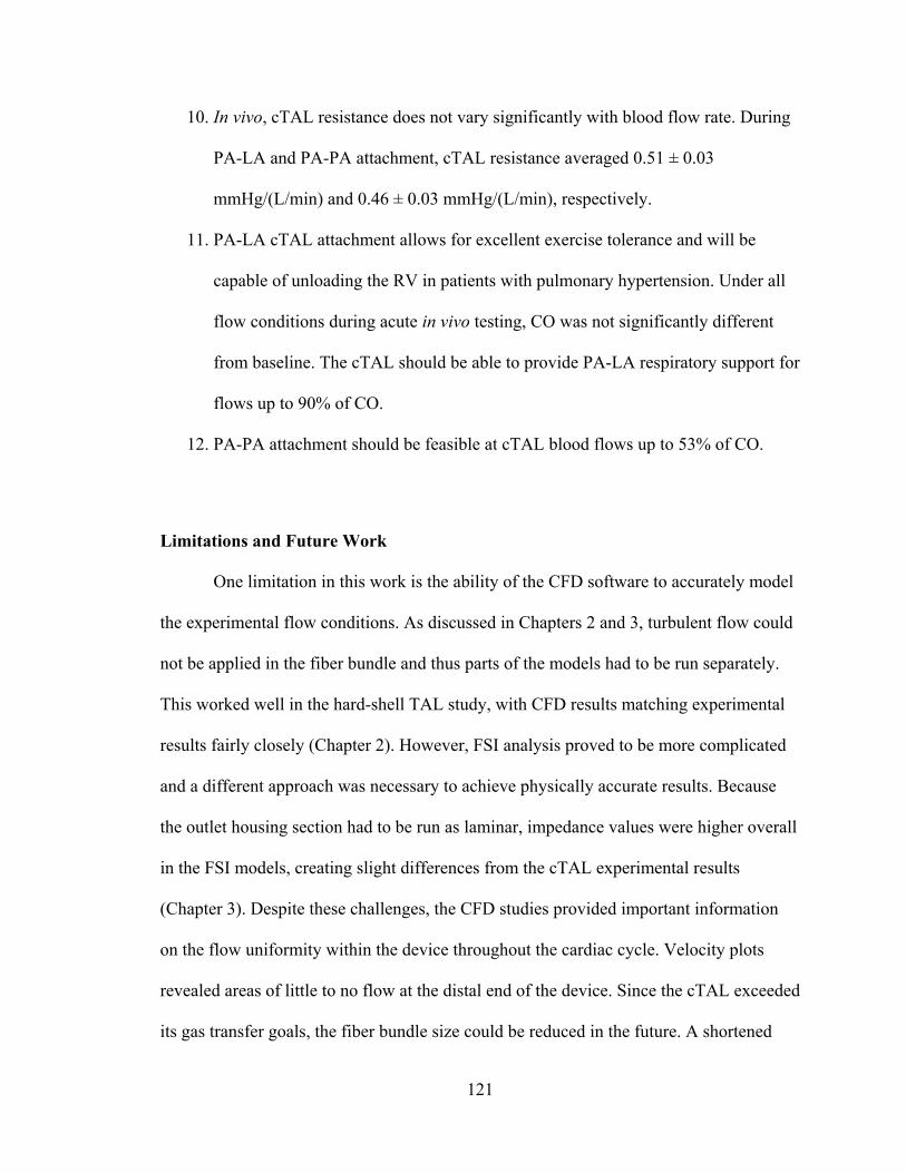
121

10. In vivo, cTAL resistance does not vary significantly with blood flow rate. During

PA-LA and PA-PA attachment, cTAL resistance averaged 0.51 ± 0.03

mmHg/(L/min) and 0.46 ± 0.03 mmHg/(L/min), respectively.

11. PA-LA cTAL attachment allows for excellent exercise tolerance and will be

capable of unloading the RV in patients with pulmonary hypertension. Under all

flow conditions during acute in vivo testing, CO was not significantly different

from baseline. The cTAL should be able to provide PA-LA respiratory support for

flows up to 90% of CO.

12. PA-PA attachment should be feasible at cTAL blood flows up to 53% of CO.

Limitations and Future Work

One limitation in this work is the ability of the CFD software to accurately model

the experimental flow conditions. As discussed in Chapters 2 and 3, turbulent flow could

not be applied in the fiber bundle and thus parts of the models had to be run separately.

This worked well in the hard-shell TAL study, with CFD results matching experimental

results fairly closely (Chapter 2). However, FSI analysis proved to be more complicated

and a different approach was necessary to achieve physically accurate results. Because

the outlet housing section had to be run as laminar, impedance values were higher overall

in the FSI models, creating slight differences from the cTAL experimental results

(Chapter 3). Despite these challenges, the CFD studies provided important information

on the flow uniformity within the device throughout the cardiac cycle. Velocity plots

revealed areas of little to no flow at the distal end of the device. Since the cTAL exceeded

its gas transfer goals, the fiber bundle size could be reduced in the future. A shortened

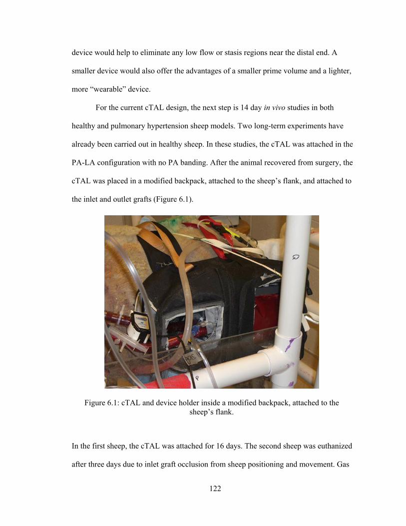
122

device would help to eliminate any low flow or stasis regions near the distal end. A

smaller device would also offer the advantages of a smaller prime volume and a lighter,

more “wearable” device.

For the current cTAL design, the next step is 14 day in vivo studies in both

healthy and pulmonary hypertension sheep models. Two long-term experiments have

already been carried out in healthy sheep. In these studies, the cTAL was attached in the

PA-LA configuration with no PA banding. After the animal recovered from surgery, the

cTAL was placed in a modified backpack, attached to the sheep’s flank, and attached to

the inlet and outlet grafts (Figure 6.1).

In the first sheep, the cTAL was attached for 16 days. The second sheep was euthanized

after three days due to inlet graft occlusion from sheep positioning and movement. Gas

Figure 6.1: cTAL and device holder inside a modified backpack, attached to the sheep’s flank.

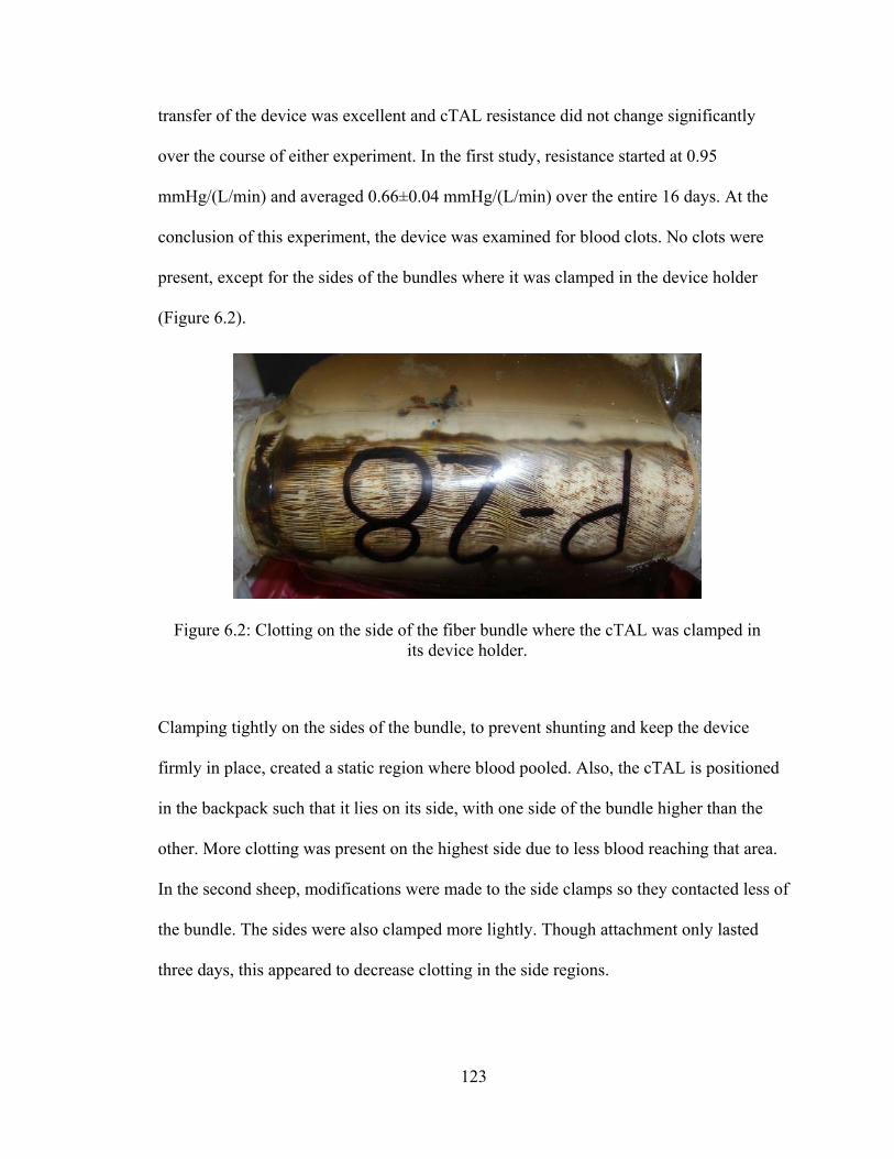
123

transfer of the device was excellent and cTAL resistance did not change significantly

over the course of either experiment. In the first study, resistance started at 0.95

mmHg/(L/min) and averaged 0.66±0.04 mmHg/(L/min) over the entire 16 days. At the

conclusion of this experiment, the device was examined for blood clots. No clots were

present, except for the sides of the bundles where it was clamped in the device holder

(Figure 6.2).

Clamping tightly on the sides of the bundle, to prevent shunting and keep the device

firmly in place, created a static region where blood pooled. Also, the cTAL is positioned

in the backpack such that it lies on its side, with one side of the bundle higher than the

other. More clotting was present on the highest side due to less blood reaching that area.

In the second sheep, modifications were made to the side clamps so they contacted less of

the bundle. The sides were also clamped more lightly. Though attachment only lasted

three days, this appeared to decrease clotting in the side regions.

Figure 6.2: Clotting on the side of the fiber bundle where the cTAL was clamped in its device holder.

124

In the future, the cTAL holder will be redesigned so the device is held in place via

attachments to the gas caps. The minimum amount of clamping necessary to prevent

shunting will be then be applied to the bundle sides. The possibility of creating internal

means of preventing shunting, which would eliminate the need for any side clamping, is

being investigated. Ultimately, long-term in vivo testing will reveal additional

information on device longevity and tolerance in different attachment configurations, as

well as different disease models.

(a)

(b)

Figure 6.3: cTAL from 3 days of attachment in a chronic sheep, using more moderate clamping of the sides. No clotting in the cTAL body (a) and reduced clotting in the

side regions (b)

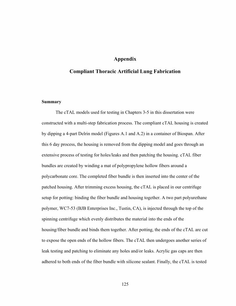
125

Appendix

Compliant Thoracic Artificial Lung Fabrication

Summary

The cTAL models used for testing in Chapters 3-5 in this dissertation were

constructed with a multi-step fabrication process. The compliant cTAL housing is created

by dipping a 4-part Delrin model (Figures A.1 and A.2) in a container of Biospan. After

this 6 day process, the housing is removed from the dipping model and goes through an

extensive process of testing for holes/leaks and then patching the housing. cTAL fiber

bundles are created by winding a mat of polypropylene hollow fibers around a

polycarbonate core. The completed fiber bundle is then inserted into the center of the

patched housing. After trimming excess housing, the cTAL is placed in our centrifuge

setup for potting: binding the fiber bundle and housing together. A two part polyurethane

polymer, WC7-53 (BJB Enterprises Inc., Tustin, CA), is injected through the top of the

spinning centrifuge which evenly distributes the material into the ends of the

housing/fiber bundle and binds them together. After potting, the ends of the cTAL are cut

to expose the open ends of the hollow fibers. The cTAL then undergoes another series of

leak testing and patching to eliminate any holes and/or leaks. Acrylic gas caps are then

adhered to both ends of the fiber bundle with silicone sealant. Finally, the cTAL is tested

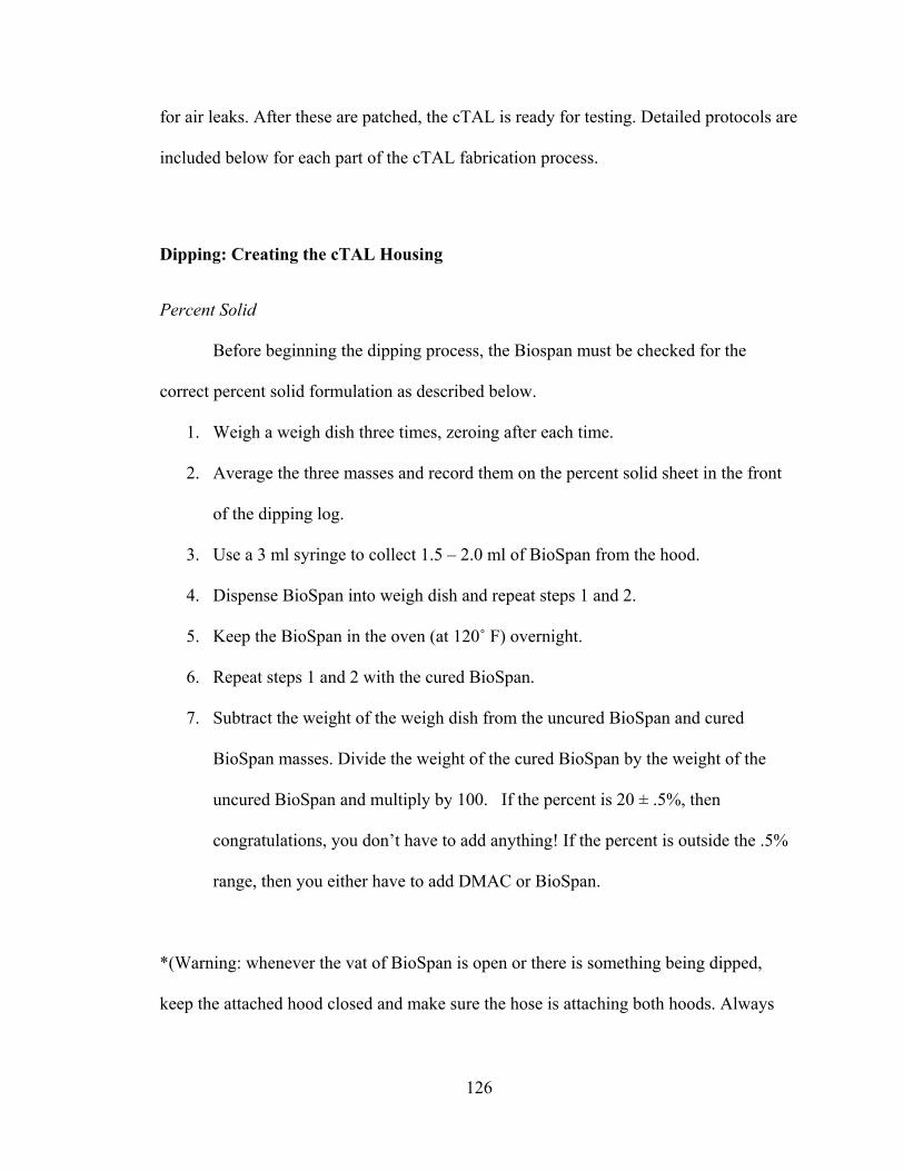
126

for air leaks. After these are patched, the cTAL is ready for testing. Detailed protocols are

included below for each part of the cTAL fabrication process.

Dipping: Creating the cTAL Housing

Percent Solid

Before beginning the dipping process, the Biospan must be checked for the

correct percent solid formulation as described below.

1. Weigh a weigh dish three times, zeroing after each time.

2. Average the three masses and record them on the percent solid sheet in the front

of the dipping log.

3. Use a 3 ml syringe to collect 1.5 – 2.0 ml of BioSpan from the hood.

4. Dispense BioSpan into weigh dish and repeat steps 1 and 2.

5. Keep the BioSpan in the oven (at 120˚ F) overnight.

6. Repeat steps 1 and 2 with the cured BioSpan.

7. Subtract the weight of the weigh dish from the uncured BioSpan and cured

BioSpan masses. Divide the weight of the cured BioSpan by the weight of the

uncured BioSpan and multiply by 100. If the percent is 20 ± .5%, then

congratulations, you don’t have to add anything! If the percent is outside the .5%

range, then you either have to add DMAC or BioSpan.

*(Warning: whenever the vat of BioSpan is open or there is something being dipped,

keep the attached hood closed and make sure the hose is attaching both hoods. Always

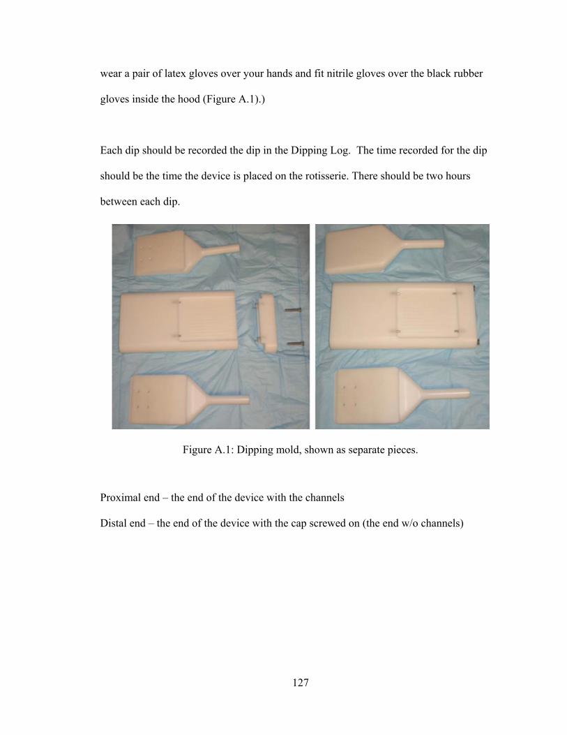
127

wear a pair of latex gloves over your hands and fit nitrile gloves over the black rubber

gloves inside the hood (Figure A.1).)

Each dip should be recorded the dip in the Dipping Log. The time recorded for the dip

should be the time the device is placed on the rotisserie. There should be two hours

between each dip.

Proximal end – the end of the device with the channels

Distal end – the end of the device with the cap screwed on (the end w/o channels)

Figure A.1: Dipping mold, shown as separate pieces.

128

Day 1 – Dipping the Proximal End of the Device (All Pieces Separate)

1. Heat dipping hood (Figure A.3) up to 120 degrees Fahrenheit with a heat gun or

another heating element. (It is easiest to set the timer the night before to start the

heat gun a minimum of two hours at the 7.5 setting before the first dip. The green

timer clip turns on the timer and the red clip turns the timer off.)

Figure A.2: Dipping mold, all pieces assembled.

Distal End

Proximal End

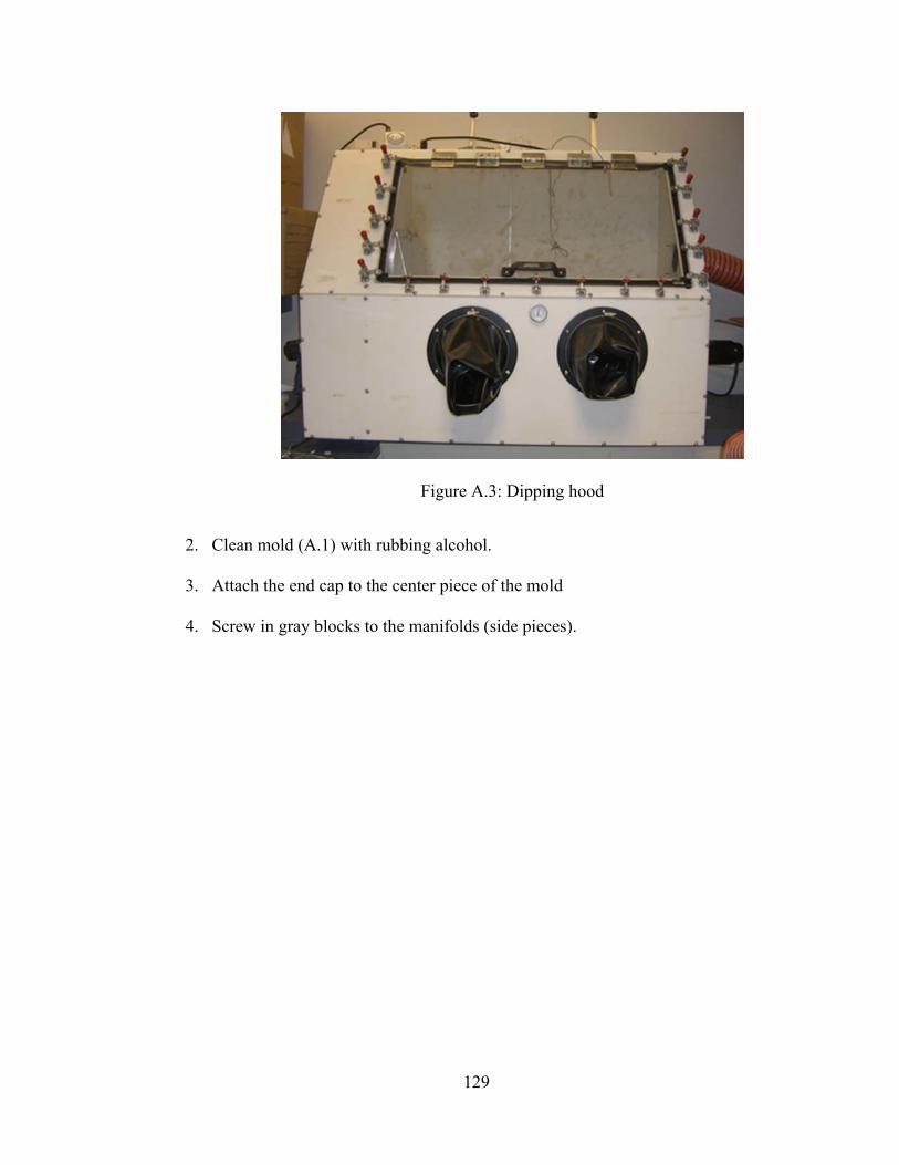
129

2. Clean mold (A.1) with rubbing alcohol.

3. Attach the end cap to the center piece of the mold

4. Screw in gray blocks to the manifolds (side pieces).

Figure A.3: Dipping hood

130

5. Attach the aluminum bar to the distal end of the center piece of the mold

6. Push the long rotisserie wire through the hole in the steel bar and secure it with

the pin (cylinder with small holes in it). Attach the other end of the wire to the

hook on the rotisserie.

7. Start the rotisserie in order to lift the center mold (keep rotisserie wire taught so

that it doesn’t get caught in the rotisserie).

8. Remove the lid from the BioSpan vat and place the vat under the device.

9. Reverse the rotisserie direction and slowly drop the mold into the BioSpan.

10. Stop the mold once the BioSpan has reached past the small steel pins (or just past

the proximal critical area).

11. Reverse the rotisserie to remove the mold from the BioSpan. When the mold

comes out of the BioSpan, immediately start a timer for four minutes as you let

excess BioSpan drip off. (It is unnecessary to leave the mold in the BioSpan for a

Figure A.4: Gray blocks attached to each housing manifold

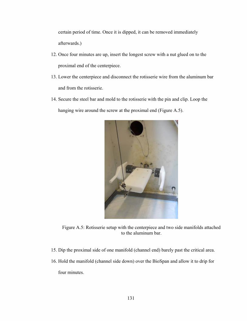
131

certain period of time. Once it is dipped, it can be removed immediately

afterwards.)

12. Once four minutes are up, insert the longest screw with a nut glued on to the

proximal end of the centerpiece.

13. Lower the centerpiece and disconnect the rotisserie wire from the aluminum bar

and from the rotisserie.

14. Secure the steel bar and mold to the rotisserie with the pin and clip. Loop the

hanging wire around the screw at the proximal end (Figure A.5).

15. Dip the proximal side of one manifold (channel end) barely past the critical area.

16. Hold the manifold (channel side down) over the BioSpan and allow it to drip for

four minutes.

Figure A.5: Rotisserie setup with the centerpiece and two side manifolds attached to the aluminum bar.

132

17. Attach the manifolds to the steel bar using the screws attached to the gray blocks

and secure them with butterfly nuts.

18. Check for bubbles after five minutes. If there are bubbles, use the dentist tools or

something sharp to pop the bubbles. Do not stop the rotisserie when popping

bubbles.

19. Wait two hours.

20. Remove steel bar from rotisserie and repeat steps 4 – 15 one time. Remember to

remove the long screw before dipping the centerpiece again.

21. Leave device on rotisserie overnight.

Day 2 – Dipping the Proximal End of the Device (All Pieces Assembled)

1. Stop rotisserie and remove device attached to aluminum bar from the hood.

2. Unscrew both manifolds from the aluminum bar and remove grey blocks.

3. Unscrew centerpiece from aluminum bar.

4. Using a scalpel, remove thin layer of BioSpan on both manifolds and centerpiece

that cured in the attachment areas.

5. Unscrew and remove distal cap from centerpiece.

6. Wipe down all pieces with rubbing alcohol.

7. Slide both manifolds into the appropriate positions on the centerpiece, followed

by the distal cap. Screw together distal cap and centerpiece to complete assembly

(Figure A.2). (Try to minimize any gaps between the manifolds and the center

piece. These make demolding difficult.)

8. Reattach the aluminum bar to the device through the holes in the distal cap.

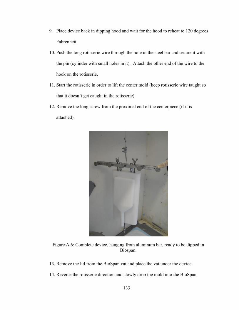
133

9. Place device back in dipping hood and wait for the hood to reheat to 120 degrees

Fahrenheit.

10. Push the long rotisserie wire through the hole in the steel bar and secure it with

the pin (cylinder with small holes in it). Attach the other end of the wire to the

hook on the rotisserie.

11. Start the rotisserie in order to lift the center mold (keep rotisserie wire taught so

that it doesn’t get caught in the rotisserie).

12. Remove the long screw from the proximal end of the centerpiece (if it is

attached).

13. Remove the lid from the BioSpan vat and place the vat under the device.

14. Reverse the rotisserie direction and slowly drop the mold into the BioSpan.

Figure A.6: Complete device, hanging from aluminum bar, ready to be dipped in Biospan.

134

15. Lower the device into the BioSpan until it is submerged to a level just past the

proximal critical area.

16. Slowly raise the device from the BioSpan. Once completely removed, stop the

rotisserie and allow it to drip while hanging for 5 minutes.

17. Place lid on BioSpan vat and set it aside.

18. Screw the long screw into the proximal side of the centerpiece.

19. Lower the device and disconnect the rotisserie wire from the aluminum bar and

from the rotisserie.

20. Secure the steel bar and mold to the rotisserie with the pin and clip. Loop the

hanging wire around the screw at the proximal end (to ensure a level rotation on

the rotisserie).

21. Start the rotisserie at the slowest speed.

22. Check for bubbles after five minutes. If there are bubbles, use the dentist tools or

something sharp to pop the bubbles. Do not stop the rotisserie when popping

bubbles.

23. Let the device cure on the rotisserie for two hours and then repeat steps 10-21 two

additional times. After the third dip, let the device cure on the rotisserie

overnight.

Day 3 – Dipping the Distal End of the Device

1. Stop the rotisserie and remove the long screw from the centerpiece.

2. Insert a short screw with nuts to both manifolds on their proximal ends.

135

3. Fit screws through holes on the cross-hook and secure the cross hook with wing

nuts on each screw.

4. Remove the device and aluminum bar from the rotisserie.

5. Hook rotisserie wire onto the cross-hook. The other end of the wire should be

attached to the hook on the rotisserie.

6. Raise the device up to a level above the vat height.

7. Remove the aluminum bar while the device is hanging.

8. Remove the lid from the BioSpan vat and place the vat under the hanging device.

9. Slowly lower the device using the rotisserie into the BioSpan vat.

10. Submerge the device in BioSpan to a level just below the proximal critical area.

11. Raise the device from the BioSpan and allow excess BioSpan to drip off of the

device for 5 minutes.

12. Place lid on BioSpan vat and set the vat aside.

13. Re-screw the aluminum bar into the distal cap of the device while it is still

hanging. (Make sure to keep pressure on the bar while screwing it in to make sure

it is tightly secured. It is okay to feel around for the holes with the screws and

touch the BioSpan at the bottom of the mold since you will be unable to see the

holes at this point.)

14. Lower the device and disconnect the rotisserie wire from the aluminum bar and

from the rotisserie.

15. Secure the steel bar and mold to the rotisserie with the pin and clip. Loop the

hanging wire around the cross hook at the proximal end (to ensure a level rotation

on the rotisserie).

136

16. Start the rotisserie at the slowest speed.

17. Check for bubbles after five minutes. If there are bubbles, use the dentist tools or

something sharp to pop the bubbles. Do not stop the rotisserie when popping

bubbles.

18. Allow the BioSpan to cure while the device is on the rotisserie for 2 hours.

19. Following 2 hours, repeat steps 4-25 four more times. On the final (fifth) dip,

allow the BioSpan to cure while the device is on the rotisserie overnight.

Day 4 – Laying the Bead

1. Shut off the heat gun.

2. Remove the device from the dipping hood.

3. Unscrew all attachments from the device (aluminum bar, short screws, and cross-

hook).

4. Wipe down the entire device with rubbing alcohol.

5. Collect a sample of BioSpan in a 3 mL syringe, attach an 18-gauge needle, and

place in the fume hood.

6. Using the syringe, lay a thick line of BioSpan (lay the bead) along one proximal

critical area, at the attachment area between the manifold and centerpiece (Figure

A.7).

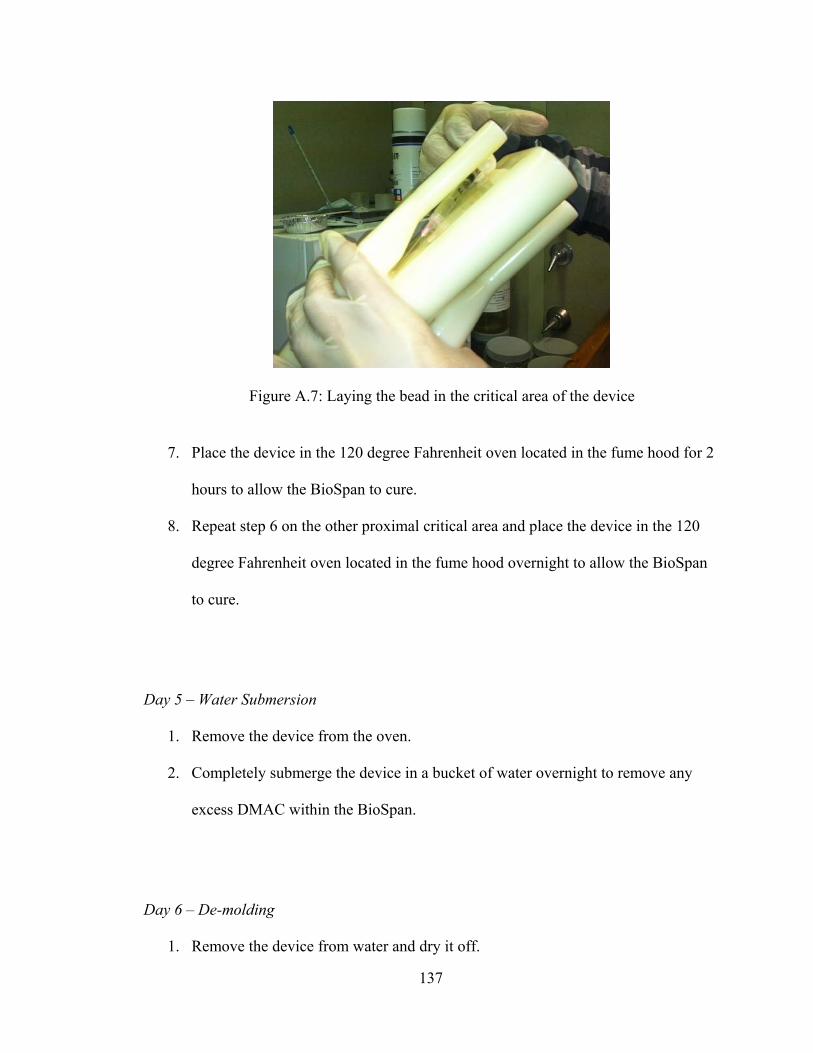
137

7. Place the device in the 120 degree Fahrenheit oven located in the fume hood for 2

hours to allow the BioSpan to cure.

8. Repeat step 6 on the other proximal critical area and place the device in the 120

degree Fahrenheit oven located in the fume hood overnight to allow the BioSpan

to cure.

Day 5 – Water Submersion

1. Remove the device from the oven.

2. Completely submerge the device in a bucket of water overnight to remove any

excess DMAC within the BioSpan.

Day 6 – De-molding

1. Remove the device from water and dry it off.

Figure A.7: Laying the bead in the critical area of the device

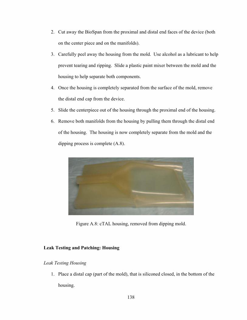
138

2. Cut away the BioSpan from the proximal and distal end faces of the device (both

on the center piece and on the manifolds).

3. Carefully peel away the housing from the mold. Use alcohol as a lubricant to help

prevent tearing and ripping. Slide a plastic paint mixer between the mold and the

housing to help separate both components.

4. Once the housing is completely separated from the surface of the mold, remove

the distal end cap from the device.

5. Slide the centerpiece out of the housing through the proximal end of the housing.

6. Remove both manifolds from the housing by pulling them through the distal end

of the housing. The housing is now completely separate from the mold and the

dipping process is complete (A.8).

Leak Testing and Patching: Housing

Leak Testing Housing

1. Place a distal cap (part of the mold), that is siliconed closed, in the bottom of the

housing.

Figure A.8: cTAL housing, removed from dipping mold.

139

2. Use medical tape to tape the housing to the cap.

3. Fold over the top of the housing and use plastic clamps to clamp shut.

4. Attach the connectors to the manifolds and zip tie in place.

5. Fill device with water from the sink. Ensure there are no air bubbles in the

device.

6. Clamp shut the tubing attached to the connectors when the device and connectors

are completely full of water.

7. When the device is completely full of water attach a pressure transducer to one of

the lure locks and ensure the other lure is closed.

8. Calibrate the transducer using the hand pump (at 0 and 300 mmHg).

9. Fill the pressure transducer and line with water

10. Take the pressure using the Biopac system

11. Check for leaks, if the device is leaking mark the leak then drain the water out of

the device by releasing the clamps

12. If the pressure is below 60 mmHg add more water using a 60 cc lure locking

syringe

13. Repeat steps 14-16 until the pressure is 60 mmHg

14. If the device has no leaks at 60 mmHg then drain the water by releasing the

clamps

15. Remove all of the tape and attachments

16. Wipe dry with paper towel

17. Let housing dry for 15 min before patching.

140

Patching Housing with Biospan

1. Wipe down the area to be patched with alcohol and allow it to dry.

2. Use a syringe to pull 1-2 ml of BioSpan from a jar of 24% BioSpan and place it

and the device in the oven (at 120˚ F) for 10 minutes to allow it to heat up.

3. If necessary, place a piece of tape on the underside of the housing to prevent

BioSpan from seeping through while patching/curing.

4. Attach a needle to the syringe and use this to apply a bead of BioSpan to the hole

in the housing.

5. Hold the housing in place for almost 15 minutes until the BioSpan sets and won’t

move once you place it into the oven.

6. Be careful with the BioSpan! If not used properly, the BioSpan will start to eat

away at the existing BioSpan – so once you place the bead onto the housing, don’t

wipe it away again!

7. Leave device in the oven overnight and the device will be ready to leak test the

next day.

Rolling Fiber Bundles

Making the fiber bundle for the compliant device is a relatively straightforward process.

One of the most important precautions to take when wrapping the fiber is to make sure

everything is sterile and stays sterile. Any unnecessary particles in the fiber have the

potential to impede flow through the device. Before beginning, make sure the bench top

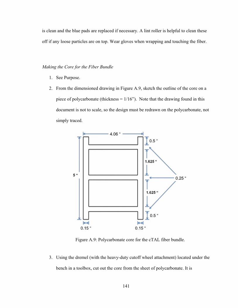
141

is clean and the blue pads are replaced if necessary. A lint roller is helpful to clean these

off if any loose particles are on top. Wear gloves when wrapping and touching the fiber.

Making the Core for the Fiber Bundle

1. See Purpose.

2. From the dimensioned drawing in Figure A.9, sketch the outline of the core on a

piece of polycarbonate (thickness = 1/16”). Note that the drawing found in this

document is not to scale, so the design must be redrawn on the polycarbonate, not

simply traced.

3. Using the dremel (with the heavy-duty cutoff wheel attachment) located under the

bench in a toolbox, cut out the core from the sheet of polycarbonate. It is

Figure A.9: Polycarbonate core for the cTAL fiber bundle.

142

important to wear safety glasses during this procedure as bits of material may fly

off.

4. Remove the backing on the polycarbonate

5. Use a piece of sandpaper to sand off any rigid marks along the sides of the core.

The edges of the core should be smooth so they do not tear the fiber when

wrapping.

6. After sanding the edges, wash the core off in the sink with water and a little bit of

rubbing alcohol.

7. Clean up the polycarbonate fragments and work area.

Wrapping the Fiber

1. See Purpose.

2. Obtain a completed core (H bracket) and wash it off with water and rubbing

alcohol.

3. Locate a ring stand with a long rod attached to it and then place the white roll of

fiber on the end of the rod.

4. Pull out a length of fiber about 16 inches long.

5. Locate the double-sided tape in one of the drawers and put a piece of this tape on

one side of the long end of the H bracket. The other side of the tape will be placed

on the end of the fiber strand you pulled out.

6. Flip the H bracket over and attach the end with tape on it to the fiber end as close

as possible to the melted edge of fiber. Make sure to place the core vertically

centered on the fiber.

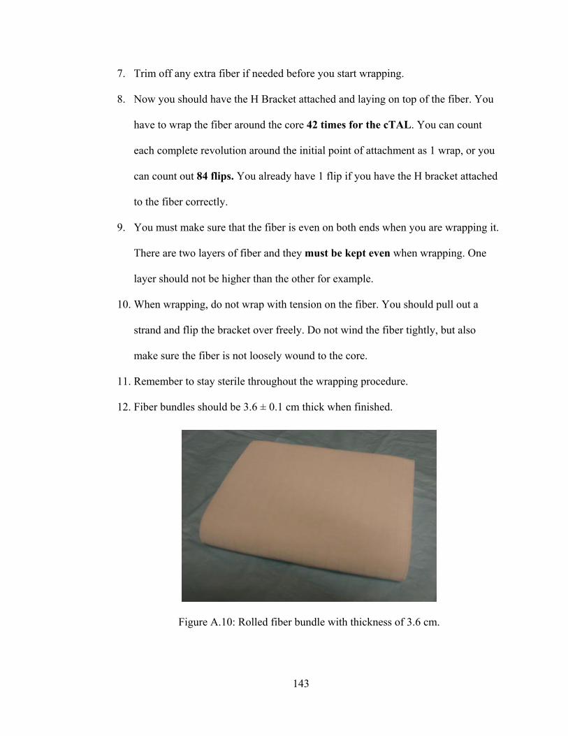
143

7. Trim off any extra fiber if needed before you start wrapping.

8. Now you should have the H Bracket attached and laying on top of the fiber. You

have to wrap the fiber around the core 42 times for the cTAL. You can count

each complete revolution around the initial point of attachment as 1 wrap, or you

can count out 84 flips. You already have 1 flip if you have the H bracket attached

to the fiber correctly.

9. You must make sure that the fiber is even on both ends when you are wrapping it.

There are two layers of fiber and they must be kept even when wrapping. One

layer should not be higher than the other for example.

10. When wrapping, do not wrap with tension on the fiber. You should pull out a

strand and flip the bracket over freely. Do not wind the fiber tightly, but also

make sure the fiber is not loosely wound to the core.

11. Remember to stay sterile throughout the wrapping procedure.

12. Fiber bundles should be 3.6 ± 0.1 cm thick when finished.

Figure A.10: Rolled fiber bundle with thickness of 3.6 cm.

144

13. Once you have completed the wrapping, locate the Impulse Sealer on the shelf of

the bench top. It is long and blue. Plug it in and turn the heating knob to 5.

14. This is used to melt the two layers of fiber into one. It is very easy to use and all

you have to do is plug it in and turn the heat knob on the right to about 4 or 5. Let

it heat for about thirty seconds.

15. Now place the completed fiber bundle on the left of the Sealer so you have

enough fiber on the right to fold up on the side of the fiber bundle without

impeding flow through the top of the bundle. If you melt the fiber too far to the

right, when you fold it up, the tape will be attached on the top side of the bundle,

ultimately impeding flow through the bundle.

16. Push the black handle of the Sealer down to melt the fiber for about 5 seconds and

release.

17. Pull about 1 inch of fiber through the sealer to melt the fiber in a second place.

18. You should now have two distinct melt “lines” on the fiber.

19. Cut closely down the edge of the first melt line closest to the wrapped bundle.

20. Now you need to attach the end of the fiber to the side of the bundle. Cut a piece

of double sided tape, put it on the side of the fiber bundle, and fold the end of

the fiber up, attaching it securely.

21. Now you have to melt the ends of the fiber bundle using a Hot Plate. It is located

on the first shelf. Plug it in and turn the heating knob to 5. It takes a couple

minutes to warm up. There should be a small, scrap plate of aluminum on top of

the Hot Plate. Leave this plate on the Hot Plate and make contact with this as

145

opposed to the Hot Plate itself when melting. This is solely for the purpose of not

accruing melted debris on the Hot Plate.

22. You need to melt the outer 10 layers or so of fiber together. Do not place the end

of the bundle on the hot plate too long or you will melt too much of the fiber.

Melt the other side of the fiber bundle.

23. Once you have melted both ends of the fiber, check for any loose particles on the

bundle and remove them. Locate a completed housing and carefully insert the

fiber bundle through the bottom of the cured compliant housing.

24. Put the completed housing with fiber bundle inserted into a large plastic bag and

into the box labeled “Complete Housings and Bundles”.

Potting: Binding the cTAL fiber bundle and housing

Preparing Devices for Potting

1. Fiber bundles should be 3.6 ± 0.1 cm thick.

2. Insert bundles into housing – try not to pull on fibers, try to keep them aligned.

3. Make sure the bundles extend a minimum of .75 inches from the critical area on

each side of the housing.

4. Trim the housing down on the proximal side until the housing no longer extends

past the bundle.

5. Fold back channels and using painter’s tape, tape them down.

146

6. Measure out one 6” x 24” piece of saran wrap and wrap around device. Use

painter’s tape to tape down the border of the saran wrap, keeping 0.75” of the

device exposed on each end.

7. Cut a triangle on both the proximal and distal ends of the device, and on the same

edge. It should be large enough that you can’t see any of the housing when

looking through the holes in the top of the potting caps.

Preparing Centrifuge

1. Wipe down potting caps with alcohol and use paper towel to grease with Grease-

It.

2. Spray all threaded rods with Grease-It under the hood.

3. Assemble cages around devices. Before tightening screws, make sure the device

is touching neither the top nor the bottom of the potting caps. Insert a micro-

spatula into top and bottom of potting caps to make sure there is sufficient room.

Also, make sure housing is in potting caps and is not folded back.

4. Hand tighten screws first, and make sure the potting caps haven’t warped when

tightening with a wrench.

5. Take four elbow connectors and two straight connectors and trim them using a

dremel so that they do not extend past the inner rims of the potting caps and the

potting tray respectively.

6. Duct tape the rim on the table where the centrifuge hood meets the table (Figure

A.11).

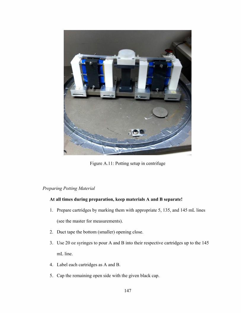
147

Preparing Potting Material

At all times during preparation, keep materials A and B separate!

1. Prepare cartridges by marking them with appropriate 5, 135, and 145 mL lines

(see the master for measurements).

2. Duct tape the bottom (smaller) opening close.

3. Use 20 oz syringes to pour A and B into their respective cartridges up to the 145

mL line.

4. Label each cartridges as A and B.

5. Cap the remaining open side with the given black cap.

Figure A.11: Potting setup in centrifuge

148

6. Tip the cartridge over when the cap is half way closed and vent the duct taped

side so that pressure does not build up inside the cartridge.

7. Snap cartridges A and B together.

8. Load the cartridges into the gun.

9. Open the tape again to allow for venting and pump the lever until the material fills

the cartridge to the 145 mL line.

a. Make sure there is an equal amount of potting material in each cartridge.

b. If material spills out of the cartridges, allow the tape to act as a barrier and

DON’T LET A AND B MIX OR THEY WILL START TO

SOLIDIFY.

10. Press the silver lever and pull back on the handle to release the pressure on the

cartridges.

11. Take the cartridges out and replace the duct tape on each.

12. Keep the cartridges in the hood when not using them.

Potting Procedure

1. Pull down the lid of the centrifuge and make sure it is locked. Go through the

safety checklist.

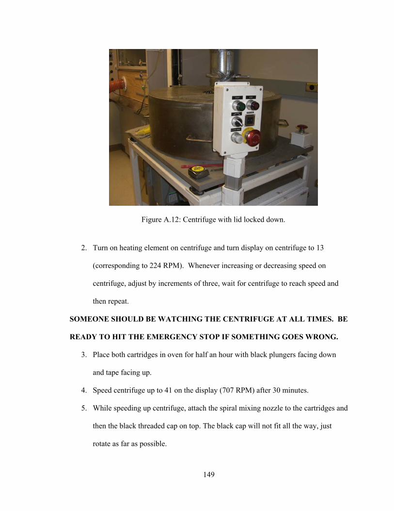
149

2. Turn on heating element on centrifuge and turn display on centrifuge to 13

(corresponding to 224 RPM). Whenever increasing or decreasing speed on

centrifuge, adjust by increments of three, wait for centrifuge to reach speed and

then repeat.

SOMEONE SHOULD BE WATCHING THE CENTRIFUGE AT ALL TIMES. BE

READY TO HIT THE EMERGENCY STOP IF SOMETHING GOES WRONG.

3. Place both cartridges in oven for half an hour with black plungers facing down

and tape facing up.

4. Speed centrifuge up to 41 on the display (707 RPM) after 30 minutes.

5. While speeding up centrifuge, attach the spiral mixing nozzle to the cartridges and

then the black threaded cap on top. The black cap will not fit all the way, just

rotate as far as possible.

Figure A.12: Centrifuge with lid locked down.

150

6. Put cartridges in caulk gun and purge 10 ml of potting material into waste tray.

7. Once 707 RPM is reached, open cover from hole in the top of the centrifuge and

inject 130 ml of potting material evenly into the middle of the white tray. Stop

with 5 ml of potting material in each cartridge. Do not allow potting material to

accumulate past the holes in the side of the tray.

8. Close cover and allow centrifuge to spin for twelve minutes at 707 RPM.

9. Purge the last 5 ml into the waste tray.

10. After twelve minutes are over, decrease speed to 13 on display. Let centrifuge

run for 48 minutes.

11. Decrease speed to 5 on display. Once it reaches 5, hit stop button. Once centrifuge

has completely stopped rotating, hit both emergency stop buttons.

12. Turn off heat gun, unplug centrifuge, and allow cooling down for 10-15 minutes.

13. Plug centrifuge back in and lift hood a few inches. Let centrifuge vent for an

hour.

14. Separate cages from centrifuge and reattach facing the opposite direction.

15. Prepare potting material and repeat potting procedure on unpotted side.

Cutting: Exposing the ends of the fibers

After removing the devices from the potting setup, the potted ends must be cut to

open up and expose the hollow fibers.

1. Measure ¼’’ in from the inside edge of the potting (on both sides) and mark with

a sharpie. This is how far in you will cut (1/4’’ of potting must remain on either

side of the cTAL after you are finished). Figure A.13.

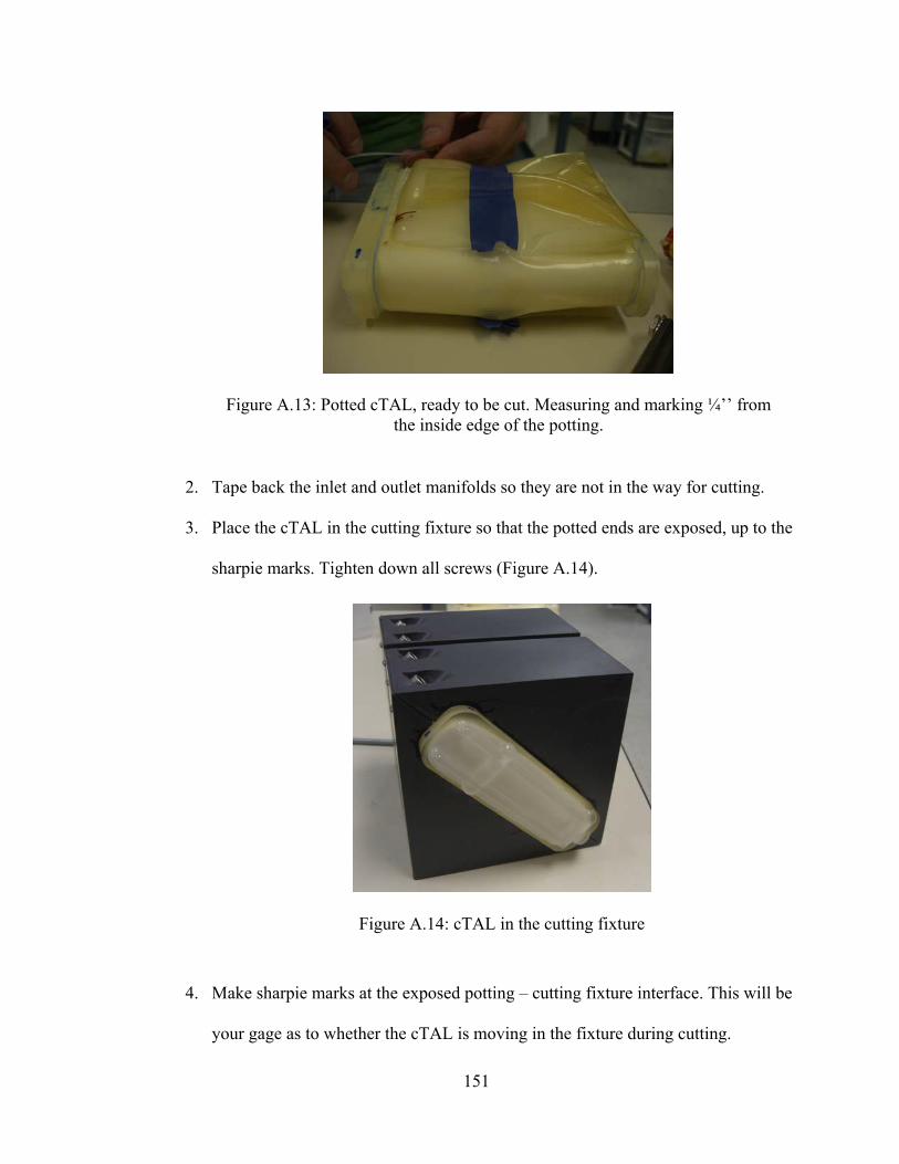
151

2. Tape back the inlet and outlet manifolds so they are not in the way for cutting.

3. Place the cTAL in the cutting fixture so that the potted ends are exposed, up to the

sharpie marks. Tighten down all screws (Figure A.14).

4. Make sharpie marks at the exposed potting – cutting fixture interface. This will be

your gage as to whether the cTAL is moving in the fixture during cutting.

Figure A.13: Potted cTAL, ready to be cut. Measuring and marking ¼’’ from the inside edge of the potting.

Figure A.14: cTAL in the cutting fixture

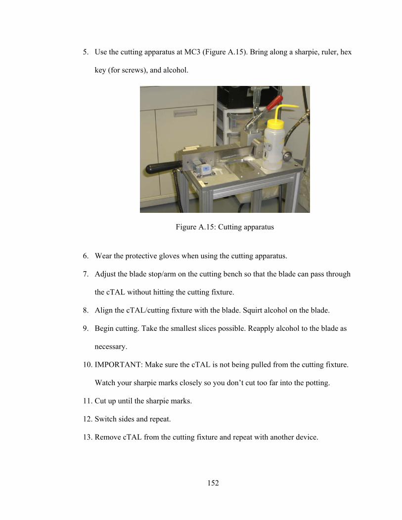
152

5. Use the cutting apparatus at MC3 (Figure A.15). Bring along a sharpie, ruler, hex

key (for screws), and alcohol.

6. Wear the protective gloves when using the cutting apparatus.

7. Adjust the blade stop/arm on the cutting bench so that the blade can pass through

the cTAL without hitting the cutting fixture.

8. Align the cTAL/cutting fixture with the blade. Squirt alcohol on the blade.

9. Begin cutting. Take the smallest slices possible. Reapply alcohol to the blade as

necessary.

10. IMPORTANT: Make sure the cTAL is not being pulled from the cutting fixture.

Watch your sharpie marks closely so you don’t cut too far into the potting.

11. Cut up until the sharpie marks.

12. Switch sides and repeat.

13. Remove cTAL from the cutting fixture and repeat with another device.

Figure A.15: Cutting apparatus

153

Leak Testing and Patching: Potted and Cut Devices

Leak Testing Cut Devices:

1. Attach connectors to manifolds and zip tie in place

2. Fill device with water from the sink.

3. When the device is completely full of water attach a pressure transducer to one of

the lure locks and ensure the other lure is closed.

4. Fill the pressure transducer and line with water and calibrate the tranducer using

the hand pump.

5. Take the pressure using the Biopac system

6. Check for leaks in both the housing and potting material, if the device is leaking

mark the leak with a permanent marker, then drain the water out of the device by

releasing the clamps

7. If the pressure is below 60 mmHg add more water using a 60 cc lure locking

syringe

8. Repeat steps 8 and 10 until the pressure is 60 mmHg

9. If the device has no leaks at 60 mmHg then drain the water by releasing the

clamps

10. Remove all of the connectors

11. Dry out device and fiber bundle using filtered air for at least 4 hours before

patching.

154

Patching Cut Devices: Housing

1. Ensure the housing or potted device is dry before patching.

2. Using a 3 cc lure lock syringe, draw up 1 mL of BioSpan from the vat in the

Dipping hood and attach an 18 gauge needle to the syringe. MAKE SURE THE

DIPPING HOOD IS CLOSED WHILE THE BIOSPAN VAT IS OPEN.

3. If necessary, tape down manifolds to keep them out of the way of the patched

holes.

4. Place device and syringe in 120 degree farenheight oven for 10 minutes to heat

up.

5. Only patch one side of the device at a time to prevent BioSpan from dripping or

spreading to unwanted areas.

6. To patch holes, dap a small amount of BioSpan onto the hole.

7. To patch slits, tape along the slit on the inside of the device. Then lay a thin line

of BioSpan along the slit.

8. Place device and syringe back in oven and let it cure for at lease 3 hours before

patching the other side and at least 12 hours before leak testing again. The

patched side of the device should be facing up.

Patching Cut Devices: Potting

1. Ensure the device is dry before patching.

2. Clean out 3, 1 mL syringes with alcohol to remove lubricant.

3. Draw up 1 mL of potting material Part A and 1 mL of potting material Part B.

4. Eject both parts of the potting material into a weigh dish and mix together.

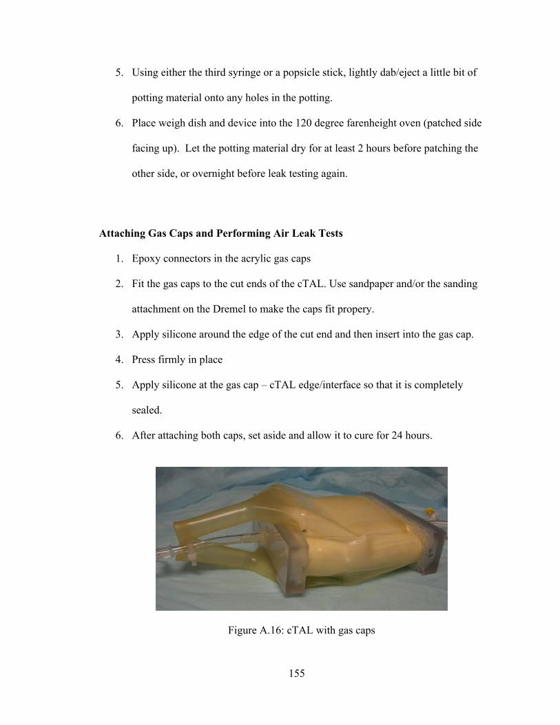
155

5. Using either the third syringe or a popsicle stick, lightly dab/eject a little bit of

potting material onto any holes in the potting.

6. Place weigh dish and device into the 120 degree farenheight oven (patched side

facing up). Let the potting material dry for at least 2 hours before patching the

other side, or overnight before leak testing again.

Attaching Gas Caps and Performing Air Leak Tests

1. Epoxy connectors in the acrylic gas caps

2. Fit the gas caps to the cut ends of the cTAL. Use sandpaper and/or the sanding

attachment on the Dremel to make the caps fit propery.

3. Apply silicone around the edge of the cut end and then insert into the gas cap.

4. Press firmly in place

5. Apply silicone at the gas cap – cTAL edge/interface so that it is completely

sealed.

6. After attaching both caps, set aside and allow it to cure for 24 hours.

Figure A.16: cTAL with gas caps

156

7. Fill a reservoir, large enough to fit the cTAL, with water.

8. Clamp the inlet and outlet of the cTAL with blue clamps so no air can escape.

9. Attach tubing to the 1.4’’ connectors on the gas caps

10. Attach the tubing to air and blow air (lightly) through the device while the device

is submerged under water.

11. Watch for air leaks from the gas caps.

12. If there are any leaks, mark them with a sharpie and then patch them with silicone

after the outside of the device is dry.

13. Allow to cure again for 24 hours and repeat gas leak testing.

14. Repeat until no air leaks remain.