Thomas G. Mezger...Thomas G. Mezger The Rheology Handbook 4th Edition ISBN 978-3-86630-650-9 eBook...
30
Thomas G. Mezger The Rheology Handbook 4 th Edition eBook European Coatings Tech Files
Transcript of Thomas G. Mezger...Thomas G. Mezger The Rheology Handbook 4th Edition ISBN 978-3-86630-650-9 eBook...

The Mission: Extremely practical coverage of the mathematical and physical principles behind rheology – from flow properties to viscoelastic behavior to taking actual measurements and interpreting them correctly. To provide a sound basis for learning about the principles of rheology and successfully applying them.
The Audience: Beginners with no previous knowledge of rheology, as well as advanced users seeking to refresh their knowledge and find out about the latest developments. For all those who seek a deeper understanding of rheology or who simply want a reference book for their daily work.
The Value: This book describes the principles of rheology clearly, vividly and in practical terms. The third edition of this standard work has been expanded to include the rheology of additives in waterbased dispersions and surfactant systems. Not only is it a great reference book, it can also serve as a textbook for studying the theory behind the methods.
Thomas G
. Mezger · The R
heology Handbook 4
th Edition
Thomas G. Mezger
The Rheology Handbook4th Edition
ISBN 978-3-86630-650-9
eBookEuropean CoatingsSymposium
European CoatingsTech Files

Thomas G. Mezger
The Rheology Handbook
For users of rotational and oscillatory rheometers
4th edition
Thomas G. Mezger: The Rheology Handbook© Copyright 2014 by Vincentz Network, Hanover, GermanyISBN 978-3-86630-650-9
Mezger, Thomas G.The Rheology Handbook, 4th EditionHanover: Vincentz Network, 2014 European Coatings Tech Files
ISBN 3-86630-650-4ISBN 978-3-86630-650-9
© 2014 Vincentz Network GmbH & Co. KG, Hanover Vincentz Network GmbH & Co. KG, Plathnerstr. 4c, 30175 Hanover, GermanyThis work is copyrighted, including the individual contributions and figures.Any usage outside the strict limits of copyright law without the consent of the publisher is prohibited and punishable by law. This especially pertains to reproduction, translation, microfilming and the storage and processing in electronic systems.The information on formulations is based on testing performed to the best of our knowledge.
Please ask for our book catalogueVincentz Network, Plathnerstr. 4c, 30175 Hanover, GermanyT +49 511 9910-033, F +49 511 [email protected], www.european-coatings.com
Layout: Vincentz Network, Hanover, GermanyPrinted by: BWH GmbH, Hanover, Germany
ISBN 3-86630-650-4ISBN 978-3-86630-650-9
Cover: Wacker Chemie, Burghausen, Germany
Bibliographische Information der Deutschen BibliothekDie Deutsche Bibliothek verzeichnet diese Publikation in der Deutschen Nationalbibliographie; detaillierte bibliographische Daten sind im Internet über http://dnb.ddb.de abrufbar.
European Coatings Tech Files
Thomas G. Mezger
The Rheology Handbook
For users of rotational and oscillatory rheometers
4th edition

Foreword
Why was this book written?People working in industry are often confronted with the effects of rheology, the science of deformation and flow behavior. When looking for appropriate literature, they find either short brochures which give only a few details and contain little useful information, or highly spe-cialized books overcharged of physical formulas and mathematical theories. There is a lack of literature between these two extremes which reduces the discussion of theoretical principles to the necessary topics, providing useful instructions for experiments on material characteriza-tion. This book is intended to fill that gap.
The practical use of rheology is presented in the following areas: quality control (QC), production and application, chemical and mechanical engineering, industrial research and development, and materials science. Emphasis is placed on current test methods related to daily working prac-tice. After reading this book, the reader should be able to perform useful tests with rotational and oscillatory rheometers, and to interpret the achieved results correctly.
How did this book come into existence?The first computer-controlled rheometers came into use in industrial laboratories in the mid 1980s. Ever since then, test methods as well as control and analysis options have improved with breath-taking speed. In order to organize and clarify the growing mountain of information, company Anton Paar Germany – and previously Physica Messtechnik – has offered basic seminars on rheology already since 1988, focused on branch-specific industrial application. During the “European Coa-tings Show” in Nuremberg in April 1999, the organizer and publishing director Dr. Lothar Vincentz suggested expanding these seminar notes into a comprehensive book about applied rheology.
What is the target audience for this book? For which industrial branches will it be most interesting?“The Rheology Handbook” is written for everyone approaching rheology without any prior knowledge, but is also useful to people wishing to update their expertise with information about recent developments. The reader can use the book as a course book and read from beginning to end or as a reference book for selected chapters. The numerous cross-references make connec-tions clear and the detailed index helps when searching. If required, the book can be used as the first step on the ladder towards theory-orientated rheology books at university level. In order to break up the text, there are as well many figures and tables, illustrative examples and small practical experiments, as well as several exercises for calculations. The following list reflects how the contents of the book are of interest to rheology users in many industrial branches.• Polymers: Solutions, melts, solids; film emulsions, cellulose solutions, latex emulsions, solid films,
sheetings, laminates; natural resins, epoxies, casting resins; silicones, caoutchouc, gums, soft and hard rubbers; thermoplastics, elastomers, thermosets, blends, foamed materials; unlinked and cross-linked polymers containing or without fillers or fibers; polymeric compounds and compo-sites; solid bars of glass-fibre, carbon-fibre and synthetic-fibre reinforced polymers (GFRP, CFRP, SFRP); polymerization, cross-linking, curing, vulcanization, melting and hardening processes
Thomas G. Mezger: The Rheology Handbook© Copyright 2014 by Vincentz Network, Hanover, GermanyISBN 978-3-86630-650-9
6
• Adhesivesandsealants: Glues, single and multi-component adhesives, pressure sensitive adhesives (PSA), UV curing adhesives, hotmelts, plastisol pastes (e.g. for automotive under-seals and seam sealings), construction adhesives, putties; uncured and cured adhesives; curing process; tack, stringiness
• Coatings,paints,lacquers: Spray, brush, dip coatings; solvent-borne, water-based coatings; metallic effect, textured, low solids, high solids, photo-resists, UV (ultra violet) radiation curing, powder coatings; glazes and stains for wood; coil coatings; solid coating films
• Printinginksandvarnishes: Gravure, letterpress, flexographic, planographic, offset, screen printing inks, UV (ultra violet) radiation curing inks; ink-jet printer inks; writing inks for pens; millbase premix, color pastes, “thixo-pastes”; liquid and pasty pigment dispersions; printing process; misting; tack
• Papercoatings: Primers and topcoats; immobilization process• Foodstuffs: Water, vegetable oils, aroma solvents, fruit juices, baby food, liquid nutrition, liqueurs,
syrups, purees, thickeners an stabilizing agents, gels, pudding, jellies, ketchup, mayonnaise, mustard, dairy products (such as yogurt, cream cheese, cheese spread, soft and hard cheese, curds, butter), emulsions, chocolate (melt), soft sweets, ice cream, chewing gum, dough, whisked egg, cappuccino foam, sausage meat, sauces containing meat chunks, jam containing fruit pieces, animal feed; bio-technological fluids; gel formation of hydrocolloids (e.g. of corn starch and gelatin); interfacial rheology (e.g. for emulsions); food tribology (e.g. for creaminess); tack
• Cosmetics,pharmaceuticals,medicaments,bio-techproducts,personalcare,healthandbeautycareproducts: Cough mixtures, perfume oils, wetting agents, nose sprays, X-ray film developing baths, blood (hemo-rheology), blood-plasma substitutes, emulsions (e.g. skin care, hair-dye), lotions, nail polish, roll-on fluids (deodorants), saliva, mucus, hydrogels, shampoo, shower gels, dispersions containing viscoelastic surfactants, skin creams, peeling creams, hair gels, styling waxes, shaving creams, tooth-gels, toothpastes, makeup disper-sions, lipsticks, mascara, ointments, vaseline, biological cells, tissue engineered medical products (TEMPs), natural and synthetic membranes, silicone pads and cushions, dental mol-ding materials, tooth filling, sponges, contact lenses, medical adhesives (for skin plasters or diapers), denture fixative creams, hair, bone cement, implants, organic-inorganic compounds (hybrids); interfacial rheology (e.g. for emulsions)
• Agrochemicals: Plant or crop protection agents, solutions and dispersions of insecticides and pesticides, herbicides and fungicides
• Detergents,homecareproducts: Household cleaning agents, liquid soap, disinfectants, surfactant solutions, washing-up liquids, dish washing agents, laundry, fabric conditioners, washing powder concentrate, fat removers; interfacial rheology
• Surfacetechnology:Polishing and abrasive suspensions; cooling emulsions• Electricalengineering,electronicsindustry: Thick film pastes, conductive, resistance,
insulating, glass paste, soft solder and screen printing pastes; SMD adhesives (for surface mounted devices), insulating and protective coatings, de-greasing agents, battery fluids and pastes, coatings for electrodes
• Petrochemicals: Crude oils, petroleum, solvents, fuels, mineral oils, light and heavy oils, lubricating greases, paraffines, waxes, petrolatum, vaseline, natural and polymer-modified bitumen, asphalt binders, distillation residues, and from coal and wood: tar and pitch; interfa-cial rheology (e.g. for emulsions)
• Ceramicsandglass: Casting slips, kaolin and porcelain suspensions, glass powder and enamel pastes, glazes, plastically deformable ceramic pastes, glass melts, aero-gels, xero-gels, sol/gel materials, composites, organo-silanes (hybrids), basalt melts
• Constructionmaterials: Self-leveling cast floors, plasters, mortar, cement suspensions, tile adhesives, dispersion paints, sealants, floor sheeting, natural and polymer-modified bitumen, asphalt binders for pavements
• Metals: Melts of magnesium, aluminum, steel, alloys; moulding process in a semi-solid state (“thixo-forming”, “thixo-casting”, “thixo-forging”), ceramic fibre reinforced light-weight metals
Foreword
7
• Wasteindustry: Waste water, sewage sludges, animal excrements (e.g. of fishes, poultry, cats, dogs, pigs), residues from refuse incineration plants
• Geology,soilmechanics,miningindustry: Soil sludges, muds; river and lake sediment masses; soil deformation due to mining operations, earthwork, canal and drain constructions; drilling fluids (e.g. containing “flow improvers”)
• Disastercontrol: Behavior of burning materials, soil deformation due to floods and earthquakes• Materialsforspecialfunctions (e.g. as “smart fluids”): Magneto-rheological fluids (MRF),
electro-rheological fluids (ERF), di-electric (DE) materials, self-repairing coatings, materials showing self-organizing superstructures (e.g. surfactants), dilatant fabrics (shock-absorbing, “shot-proof”), liquid crystals (LC), ionic fluids, micro-capsule paraffin wax (e.g. as “phase-change material” PCM)
It is pleasing that the first two editions of “The Rheology Handbook”, published in 2002 and 2006, sold out so unexpectedly quickly. It was positive to hear that the book met with approval, not only from laboratory technicians and practically oriented engineers, but also from teachers and professors of schools and colleges of applied sciences. Even at universities, “The Rheology Handbook” is meanwhile taken as an introductory teaching material for explaining the basics of rheology in lectures and practical courses, and as a consequence, many students worldwide are using it when writing their final paper or thesis.
Also for the third edition, further present-day examples have been added resulting as well from contacts to industrial users as well as from corporation with several working groups, e.g. for developing modern standardizing measuring methods for diverse industrial branches. Here in a nutshell, the following additional chapters of this new edition are: Types of flow in the Two-Plates-Model (Chapter 2.4), the effects of rheological additives in aqueous dispersions (Chapter 3.3.7), SAOS and LAOS tests and Lissajous diagrams (Chapter 8.3.6), nano-structures and com-plex rheological behavior such as shear-banding explained by using surfactant systems as an example (Chapter 9), and special measuring devices for rheo-optical systems and extensional tests (Chapter 10.8). Also the references and standards have been updated (Chapter 14). This textbook is also available in German language, and also here, four editions were published up to now, in 2000, 2006, 2010 and in September 2012 (title: “Das Rheologie Handbuch”).
I hope that “The Rheology Handbook” will prove itself a useful source of information for cha-racterizing the above mentioned products in an application-oriented way, assuring their quality and helping to improve them wherever possible.
AcknowledgementsI would like to say a big “Thank You” to all those people without whose competent ideas and suggestions for improvement it would not have been possible to produce such a comprehen-sive and understandable book. The following people have been of special help to me: Heike Audehm, Monika Bernzen, Stefan Büchner, Marcel de Pender, Gerd Dornhöfer, Andreas Eich, Elke Fischle, Ingrid Funk, Patrick Heyer, Siegfried Huck, Jörg Läuger, Thomas Litters, Sabine Neuber, Matthias Prenzel, Hubert Reitberger, Michael Ringhofer, Oliver Sack, Michael Schäffler, Carmen Schönhaar, Werner Stehr, Heiko Stettin, Jürgen Utz, Detlef van Peij, Simone Will and Klaus Wollny. Sarah Knights translated the original German text into English. Besides the sup-port of my colleagues worldwide, I would also like to mention the managers of Anton Paar GmbH in Graz, Austria, and Anton Paar Germany GmbH in Ostfildern (near Stuttgart).
Stuttgart, April 2014
Thomas G. Mezger
Foreword

Born to find out
The New MCR Series: Modular Rheometers Ready for Everything
Whatever your rheological requirements are and will be in the future – MCR rheometers are always efficiently and comfortably adapted to meet your needs.
Find out more about the MCR rheometer series at www.anton-paar.com.
Anton Paar® [email protected]
MCRxx2_165x260.indd 1 12.05.14 11:10
Contents 9
Contents
1 Introduction ............................................................................................ 171.1 Rheology, rheometry and viscoelasticity ................................................................. 171.2 Deformation and flow behavior ................................................................................... 18
2 Flowbehaviorandviscosity ................................................................... 212.1 Introduction ...................................................................................................................... 212.2 Definition of terms ......................................................................................................... 212.2.1 Shear stress ...................................................................................................................... 222.2.2 Shear rate .......................................................................................................................... 222.2.3 Viscosity ............................................................................................................................ 262.3 Shear load-dependent flow behavior ........................................................................ 292.3.1 Ideally viscous flow behavior according to Newton .............................................. 292.4 Types of flow illustrated by the Two-Plates Model ......................................................31
3 Rotational tests ........................................................................................ 333.1 Introduction ...................................................................................................................... 333.2 Basic principles ............................................................................................................... 333.2.1 Test modes controlled shear rate (CSR) and controlled shear stress (CSS),
raw data and rheological parameters ........................................................................ 333.3 Flow curves and viscosity functions ......................................................................... 343.3.1 Description of the test .................................................................................................... 343.3.2 Shear-thinning flow behavior ..................................................................................... 383.3.2.1 Structures of polymers showing shear-thinning behavior ................................. 393.3.2.2 Structures of dispersions showing shear-thinning behavior ............................. 443.3.3 Shear-thickening flow behavior .................................................................................. 443.3.3.1 Structures of polymers showing shear-thickening behavior ............................. 483.3.3.2 Structures of dispersions showing shear-thickening behavior ......................... 493.3.4 Yield point ......................................................................................................................... 493.3.4.1 Yield point determination using the flow curve diagram .................................... 503.3.4.2 Yield point determination using the shear stress/deformation diagram ......... 513.3.4.3 Further information on yield points .......................................................................... 533.3.5 Overview: Flow curves and viscosity functions ..................................................... 573.3.6 Fitting functions for flow and viscosity curves ...................................................... 583.3.6.1 Model function for ideally viscous flow behavior ................................................... 593.3.6.2 Model functions for shear-thinning and shear-thickening flow behavior ..... 593.3.6.3 Model functions for flow behavior with zero-shear and infinite-shear
viscosity ............................................................................................................................ 603.3.6.4 Model functions for flow curves with a yield point ............................................... 613.3.7 The effects of rheological additives in aqueous dispersions ............................... 643.4 Time-dependent flow behavior and viscosity function ......................................... 683.4.1 Description of the test .................................................................................................... 683.4.2 Time-dependent flow behavior of samples showing no hardening ................... 693.4.2.1 Structural decomposition and regeneration (thixotropy and rheopexy) ......... 70
Thomas G. Mezger: The Rheology Handbook© Copyright 2014 by Vincentz Network, Hanover, GermanyISBN 978-3-86630-650-9
Contents10
3.4.2.2 Test methods for investigating thixotropic behavior ............................................ 723.4.3 Time-dependent flow behavior of samples showing hardening ......................... 793.5 Temperature-dependent flow behavior and viscosity function .......................... 803.5.1 Description of the test .................................................................................................... 803.5.2 Temperature-dependent flow behavior of samples showing no hardening ....... 813.5.3 Temperature-dependent flow behavior of samples showing hardening .......... 823.5.4 Fitting functions for curves of the temperature-dependent viscosity ............. 833.6 Pressure-dependent flow behavior and viscosity function ................................. 85
4 Elasticbehaviorandshearmodulus ..................................................... 894.1 Introduction ...................................................................................................................... 894.2 Definition of terms ......................................................................................................... 894.2.1 Deformation and strain ................................................................................................. 894.2.2 Shear modulus ................................................................................................................. 904.3 Shear load-dependent deformation behavior ........................................................... 934.3.1 Ideally elastic deformation behavior according to Hooke .................................... 93
5 Viscoelasticbehavior .............................................................................. 975.1 Introduction ...................................................................................................................... 975.2 Basic principles ............................................................................................................... 975.2.1 Viscoelastic liquids according to Maxwell .............................................................. 975.2.1.1 Maxwell model ................................................................................................................ 975.2.1.2 Examples of the behavior of VE liquids in practice ............................................... 995.2.2 Viscoelastic solids according to Kelvin/Voigt ........................................................ 1025.2.2.1 Kelvin/Voigt model ........................................................................................................ 1025.2.2.2 Examples of the behavior of VE solids in practice ................................................. 1045.3 Normal stresses .............................................................................................................. 106
6 Creeptests ............................................................................................... 1096.1 Introduction ...................................................................................................................... 1096.2 Basic principles ............................................................................................................... 1096.2.1 Description of the test .................................................................................................... 1096.2.2 Ideally elastic behavior ................................................................................................. 1106.2.3 Ideally viscous behavior ............................................................................................... 1116.2.4 Viscoelastic behavior ..................................................................................................... 1116.3 Analysis ............................................................................................................................. 1126.3.1 Behavior of the molecules............................................................................................. 1126.3.2 Burgers model ................................................................................................................. 1126.3.3 Curve discussion ............................................................................................................ 1136.3.4 Definition of terms ......................................................................................................... 1166.3.4.1 Zero-shear viscosity ....................................................................................................... 1166.3.4.2 Creep compliance, and creep recovery compliance .............................................. 1176.3.4.3 Retardation time ............................................................................................................. 1186.3.4.4 Retardation time spectrum .......................................................................................... 1196.3.5 Data conversion ............................................................................................................... 1216.3.6 Determination of the molar mass distribution ........................................................ 122
7 Relaxation tests ....................................................................................... 1237.1 Introduction ...................................................................................................................... 1237.2 Basic principles ............................................................................................................... 1237.2.1 Description of the test .................................................................................................... 123
Contents 11
7.2.2 Ideally elastic behavior ................................................................................................. 1247.2.3 Ideally viscous behavior ............................................................................................... 1257.2.4 Viscoelastic behavior ..................................................................................................... 1257.3 Analysis ............................................................................................................................. 1267.3.1 Behavior of the molecules............................................................................................. 1267.3.2 Curve discussion ............................................................................................................ 1277.3.3 Definition of terms ......................................................................................................... 1287.3.3.1 Relaxation modulus ........................................................................................................ 1287.3.3.2 Relaxation time ............................................................................................................... 1297.3.3.3 Relaxation time spectrum ............................................................................................ 1307.3.4 Data conversion ............................................................................................................... 1327.3.5 Determination of the molar mass distribution ........................................................ 134
8 Oscillatory tests ...................................................................................... 1358.1 Introduction ...................................................................................................................... 1358.2 Basic principles ............................................................................................................... 1358.2.1 Ideally elastic behavior ................................................................................................. 1368.2.2 Ideally viscous behavior ............................................................................................... 1388.2.3 Viscoelastic behavior ..................................................................................................... 1388.2.4 Definition of terms ......................................................................................................... 1398.2.5 The test modes controlled shear strain and controlled shear stress,
raw data and rheological parameters ....................................................................... 1448.3 Amplitude sweeps .......................................................................................................... 1468.3.1 Description of the test .................................................................................................... 1468.3.2 Structural character of a sample ................................................................................ 1468.3.3 Limiting value of the LVE range ................................................................................. 1488.3.3.1 Limiting value of the LVE range in terms of the shear strain ........................... 1488.3.3.2 Limiting value of the LVE range in terms of the shear stress ............................ 1518.3.4 Determination of the yield point and the flow point by amplitude sweeps ..... 1518.3.4.1 Yield point or yield stress τy ......................................................................................... 1518.3.4.2 Flow point or flow stress τf ........................................................................................... 1528.3.4.3 Yield zone between yield point and flow point ....................................................... 1528.3.4.4 Evaluation of the two terms yield point and flow point ........................................ 1538.3.4.5 Measuring programs in combination with amplitude sweeps .......................... 1538.3.5 Frequency-dependence of amplitude sweeps ......................................................... 1548.3.6 SAOS and LAOS tests, and Lissajous diagrams ...................................................... 1558.4 Frequency sweeps .......................................................................................................... 1598.4.1 Description of the test .................................................................................................... 1608.4.2 Behavior of unlinked polymers (solutions and melts)........................................... 1618.4.2.1 Single Maxwell model for unlinked polymers showing a narrow MMD ......... 1618.4.2.2 Generalized Maxwell model for unlinked polymers showing a wide MMD .. 1658.4.3 Behavior of cross-linked polymers ............................................................................. 1688.4.4 Behavior of dispersions and gels ................................................................................ 1718.4.5 Comparison of superstructures using frequency sweeps ................................... 1748.4.6 Multiwave test ................................................................................................................. 1748.4.7 Data conversion ............................................................................................................... 1768.5 Time-dependent behavior at constant dynamic-mechanical and
isothermal conditions .................................................................................................... 1768.5.1 Description of the test .................................................................................................... 1768.5.2 Time-dependent behavior of samples showing no hardening ............................ 1778.5.2.1 Structural decomposition and regeneration (thixotropy and rheopexy) ......... 178
Contents12
8.5.2.2 Test methods for investigating thixotropic behavior ............................................ 1798.5.3 Time-dependent behavior of samples showing hardening .................................. 1858.6 Temperature-dependent behavior at constant dynamic mechanical
conditions .......................................................................................................................... 1888.6.1 Description of the test .................................................................................................... 1898.6.2 Temperature-dependent behavior of samples showing no hardening ............. 1908.6.2.1 Temperature curves and structures of polymers ................................................... 1908.6.2.2 Temperature-curves of dispersions and gels .......................................................... 1978.6.3 Temperature-dependent behavior of samples showing hardening ................... 2008.6.4 Thermoanalysis (TA) ...................................................................................................... 2028.7 Time/temperature shift................................................................................................. 2038.7.1 Temperature shift factor according to the WLF method ...................................... 2048.8 The Cox/Merz relation .................................................................................................. 2098.9 Combined rotational and oscillatory tests ................................................................ 2108.9.1 Presetting rotation and oscillation in series ............................................................ 2108.9.2 Superposition of oscillation and rotation ................................................................. 210
9 Complexbehavior,surfactantsystems .................................................. 2139.1 Surfactant systems ......................................................................................................... 2139.1.1 Surfactant structures and micelles ........................................................................... 2139.1.2 Emulsions ......................................................................................................................... 2229.1.3 Mixtures of surfactants and polymers, surfactant-like polymers ..................... 2239.1.4 Applications of surfactant systems ............................................................................ 2259.2 Rheological behavior of surfactant systems ............................................................ 2269.2.1 Typical shear behavior .................................................................................................. 2269.2.2 Shear-induced effects, shear-banding and “rheo chaos” ..................................... 229
10 Measuring systems ................................................................................. 23310.1 Introduction ...................................................................................................................... 23310.2 Concentric cylinder measuring systems (CC MS) ................................................. 23310.2.1 Cylinder measuring systems in general .................................................................. 23310.2.1.1 Geometry of cylinder measuring systems showing a large gap ........................ 23310.2.1.2 Operating methods ......................................................................................................... 23310.2.1.3 Calculations ...................................................................................................................... 23410.2.2 Narrow-gap concentric cylinder measuring systems according to ISO 3219 ..... 23510.2.2.1 Geometry of ISO cylinder systems ............................................................................. 23510.2.2.2 Calculations ...................................................................................................................... 23710.2.2.3 Conversion between raw data and rheological parameters ................................. 23810.2.2.4 Flow instabilities and secondary flow effects in cylinder measuring systems .. 23810.2.2.5 Advantages and disadvantages of cylinder measuring systems ....................... 24010.2.3 Double-gap measuring systems (DG MS) ................................................................ 24110.2.4 High-shear cylinder measuring systems (HS MS) ................................................ 24110.3 Cone-and-plate measuring systems (CP MS) .......................................................... 24210.3.1 Geometry of cone-and-plate systems ........................................................................ 24210.3.2 Calculations ...................................................................................................................... 24210.3.3 Conversion between raw data and rheological parameters ................................ 24410.3.4 Flow instabilities and secondary flow effects in CP systems ............................. 24410.3.5 Cone truncation and gap setting ................................................................................ 24410.3.6 Maximum particle size ................................................................................................. 24510.3.7 Filling of the cone-and-plate measuring system .................................................... 24610.3.8 Advantages and disadvantages of cone-and-plate measuring systems ........... 246
Contents 13
10.4 Parallel-plate measuring systems (PP MS) .............................................................. 24810.4.1 Geometry of parallel-plate systems ........................................................................... 24810.4.2 Calculations ...................................................................................................................... 24910.4.3 Conversion between raw data and rheological parameters ................................. 25010.4.4 Flow instabilities and secondary flow effects in a PP system ............................ 25110.4.5 Recommendations for gap setting ............................................................................. 25110.4.6 Automatic gap setting and automatic gap control using the normal force
control option ................................................................................................................... 25110.4.7 Determination of the temperature gradient in the sample .................................. 25210.4.8 Advantages and disadvantages of parallel-plate measuring systems ............. 25210.5 Mooney/Ewart measuring systems (ME MS) ......................................................... 25410.6 Relative measuring systems ........................................................................................ 25510.6.1 Measuring systems with sandblasted, profiled or serrated surfaces ............... 25510.6.2 Spindles in the form of disks, pins, and spheres .................................................... 25610.6.3 Krebs spindles or paddles ............................................................................................ 25910.6.4 Paste spindles and rotors showing pins and vanes ............................................... 26010.6.5 Ball measuring systems, performing rotation on a circular line ....................... 26110.6.6 Further relative measuring systems ......................................................................... 26210.7 Measuring systems for solid torsion bars ................................................................ 26210.7.1 Bars showing a rectangular cross section .............................................................. 26310.7.2 Bars showing a circular cross section....................................................................... 26510.7.3 Composite materials ...................................................................................................... 26610.8 Special measuring devices .......................................................................................... 26710.8.1 Special measuring conditions which influence rheology .................................... 26710.8.1.1 Magnetic fields for magneto-rheological fluids ...................................................... 26710.8.1.2 Electrical fields for electro-rheological fluids .......................................................... 26810.8.1.3 Immobilization of suspensions by extraction of fluid ........................................... 26810.8.1.4 UV light for UV-curing materials............................................................................... 26910.8.2 Rheo-optical measuring devices ................................................................................ 26910.8.2.1 Terms from optics ........................................................................................................... 27010.8.2.2 Microscopy ....................................................................................................................... 27410.8.2.3 Devices for measuring anisotropy in terms of optical rotation and
birefringence ................................................................................................................... 27510.8.2.4 SALS for diffracted light quanta ................................................................................. 27510.8.2.5 SAXS for diffracted X-rays ........................................................................................... 27610.8.2.6 SANS for scattered neutrons ....................................................................................... 27710.8.2.7 Velocity profile of flow fields ........................................................................................ 27810.8.3 Other special measuring devices ............................................................................... 27810.8.3.1 Interfacial rheology on two-dimensional liquid films .......................................... 27810.8.3.2 Dielectric analysis, and DE conductivity of materials showing electric
dipoles ................................................................................................................................ 27810.8.3.3 NMR, and resonance of magnetically active atomic nuclei ................................. 28010.8.4 Other kinds of testings besides shear tests ............................................................ 28010.8.4.1 Tensile tests, extensional viscosity, and extensional rheology ........................... 28010.8.4.2 Tack test, stickiness and tackiness ........................................................................... 28410.8.4.3 Tribology ........................................................................................................................... 287
11 Instruments ............................................................................................. 29111.1 Introduction ...................................................................................................................... 29111.2 Short overview: methods for testing viscosity and elasticity ............................. 29111.2.1 Very simple determinations ......................................................................................... 291
Contents14
11.2.2 Flow on a horizontal plane ........................................................................................... 29211.2.3 Spreading or slump on a horizontal plane after lifting a container .................. 29311.2.4 Flow on an inclined plane ............................................................................................. 29411.2.5 Flow on a vertical plane or over a special tool ......................................................... 29411.2.6 Flow in a channel, trough or bowl .............................................................................. 29511.2.7 Flow cups and other pressureless capillary viscometers .................................... 29611.2.8 Devices showing rising, sinking, falling and rolling elements ........................ 29611.2.9 Penetrometers, consistometers and texture analyzers ........................................ 29811.2.10 Pressurized cylinder and capillary devices ............................................................ 30011.2.11 Simple rotational viscometer tests ............................................................................. 30111.2.12 Devices with vibrating or oscillating elements ...................................................... 30411.2.13 Rotational and oscillatory curemeters (for rubber testing) ................................. 30511.2.14 Tension testers ................................................................................................................ 30711.2.15 Compression testers ...................................................................................................... 30811.2.16 Linear shear testers ...................................................................................................... 30811.2.17 Bending or flexure testers ........................................................................................... 30811.2.18 Torsion testers ................................................................................................................. 30911.3 Flow cups .......................................................................................................................... 31011.3.1 ISO cup .............................................................................................................................. 31111.3.1.1 Capillary length .............................................................................................................. 31111.3.1.2 Calculations ...................................................................................................................... 31211.3.1.3 Flow instabilities, secondary flow effects, turbulent flow conditions in
flow cups ........................................................................................................................... 31311.3.2 Other types of flow cups ............................................................................................... 31411.4 Capillary viscometers .................................................................................................... 31511.4.1 Glass capillary viscometers ......................................................................................... 31511.4.1.1 Calculations ...................................................................................................................... 31711.4.1.2 Determination of the molar mass of polymers using diluted polymer
solutions ............................................................................................................................ 31911.4.1.3 Determination of the viscosity index VI of petrochemicals ............................... 32311.4.2 Pressurized capillary viscometers ............................................................................ 32411.4.2.1 MFR and MVR testers driven by a weight (“low-pressure capillary
viscometers”) ................................................................................................................... 32411.4.2.2 High-pressure capillary viscometers driven by an electric drive,
for testing highly viscous and paste-like materials ............................................. 32911.4.2.3 High-pressure capillary viscometers driven by gas pressure,
for testing liquids ........................................................................................................... 33211.5 Falling-ball viscometers ............................................................................................... 33411.6 Rotational and oscillatory rheometers ....................................................................... 33511.6.1 Rheometer set-ups .......................................................................................................... 33711.6.2 Control loops .................................................................................................................... 33811.6.3 Devices to measure torques ......................................................................................... 34111.6.4 Devices to measure deflection angles and rotational speeds ............................. 34211.6.5 Bearings ............................................................................................................................ 34311.6.6 Temperature control systems ...................................................................................... 344
12 Guideline for rheological tests ............................................................... 34912.1 Selection of the measuring system ............................................................................ 34912.2 Rotational tests ................................................................................................................ 34912.2.1 Flow and viscosity curves ............................................................................................ 34912.2.2 Time-dependent flow behavior (rotation) ................................................................. 350
Contents 15
12.2.3 Step tests (rotation): structural decomposition and regeneration (“thixotropy”) ................................................................................................................... 350
12.2.4 Temperature-dependent flow behavior (rotation) ................................................... 35112.3 Oscillatory tests ............................................................................................................... 35112.3.1 Amplitude sweeps .......................................................................................................... 35112.3.2 Frequency sweeps .......................................................................................................... 35112.3.3 Time-dependent viscoelastic behavior (oscillation) ............................................... 35212.3.4 Step tests (oscillation): structural decomposition and regeneration
(“thixotropy”) ................................................................................................................... 35212.3.5 Temperature-dependent viscoelastic behavior (oscillation) ................................ 35312.4 Selection of the test type .............................................................................................. 35412.4.1 Behavior at rest ............................................................................................................... 35412.4.2 Flow behavior ................................................................................................................... 35512.4.3 Structural decomposition and regeneration (“thixotropic behavior”,
e.g. of coatings) ................................................................................................................ 355
13 Rheologistsandthehistoricaldevelopmentofrheology ..................... 35713.1 Development until the 19th century ........................................................................... 35713.2 Development between 1800 and 1900 ...................................................................... 36013.3 Development between 1900 and 1949 ...................................................................... 36713.4 Development between 1950 and 1979 ....................................................................... 37613.5 Development since 1980 ............................................................................................... 379
14 Appendix ................................................................................................. 38314.1 Symbols, signs and abbreviations used .................................................................... 38314.2 The Greek alphabet ........................................................................................................ 39114.3 Conversion table for units ............................................................................................. 391
15 References ............................................................................................... 39515.1 Publications and books ................................................................................................. 39515.2 ISO standards .................................................................................................................. 40715.3 ASTM standards ............................................................................................................ 40915.4 DIN, DIN EN, DIN EN ISO and EN standards .......................................................... 41415.5 Important standards for users of rotational rheometers ...................................... 417
Author ...................................................................................................... 418
Index ........................................................................................................ 419

European Coatings Tech Shelf
Do you prefer reading a digital edition of European Coatings Journal? Or are you searching for eBooks on coatings technology? Now you can have both – thanks to the European Coatings Tech Shelf!
Keep up with all the expert knowledge you need – anytime, anywhere, on your mobile device
Already a subscriber to European Coatings Journal? Then enjoy free access to all current issues of the eJournal as well as to the editorial archives.
See the complete range of European Coatings eBooks at a glance – and browse inside to find exactly the information you need.
Vincentz Network · Tel. +49 511 9910-025 · [email protected] · www.european-coatings.com
Grab the App!Your mobile source for coatings technology information
Sponsored by
Scan the code below with your iPad or iPhone, or simply enter the
URL address into your browser. (For subscribers: please enter
your subscription number in the ‘settings‘ menu of the app.)
www.european-coatings.com/techshelf
Here‘s how!
17Rheology, rheometry and viscoelasticity
Thomas G. Mezger: The Rheology Handbook© Copyright 2014 by Vincentz Network, Hanover, GermanyISBN 978-3-86630-650-9
1 Introduction
1.1 Rheology, rheometry and viscoelasticitya) Rheology
Rheology is the science of deformation and flow. It is a branch of physics and physical chemi-stry since the most important variables come from the field of mechanics: forces, deflections and velocities. The term “rheology” originates from the Greek: “rhein” meaning “to flow”. Thus, rheology is literally “flow science”. However, rheological experiments do not merely reveal information about flow behavior of liquids but also about deformation behavior of solids. The connection here is that a large deformation produced by shear forces causes many materials to flow.
All kinds of shear behavior, which can be described rheologically in a scientific way, can be viewed as being in between two extremes: flow of ideally viscous liquids on the one hand and deformation of ideally elastic solids on the other. Two illustrative examples for the extremes of ideal behavior are low-viscosity mineral oils and rigid steel balls. Flow behavior of ideally viscous fluids is explained in Chapter 2. Ideally elastic deformation behavior is described in Chapter 4.
Behavior of all real materials is based on the combination of both a viscous and an elastic por-tion and therefore, it is called viscoelastic. Wallpaper paste is a viscoelastic liquid, for example, and a gum eraser is a viscoelastic solid. Information on viscoelastic behavior can be found in Chapter 5. Complex and extraordinary rheological behavior is presented in Chapter 9 using the example of surfactant systems.
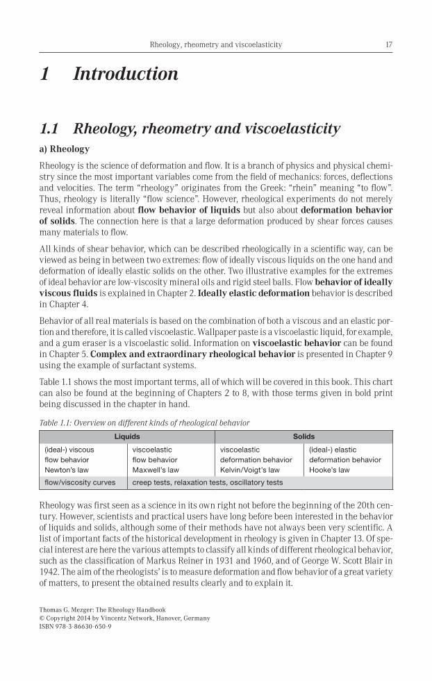
Table 1.1 shows the most important terms, all of which will be covered in this book. This chart can also be found at the beginning of Chapters 2 to 8, with those terms given in bold print being discussed in the chapter in hand.
Rheology was first seen as a science in its own right not before the beginning of the 20th cen-tury. However, scientists and practical users have long before been interested in the behavior of liquids and solids, although some of their methods have not always been very scientific. A list of important facts of the historical development in rheology is given in Chapter 13. Of spe-cial interest are here the various attempts to classify all kinds of different rheological behavior, such as the classification of Markus Reiner in 1931 and 1960, and of George W. Scott Blair in 1942. The aim of the rheologists’ is to measure deformation and flow behavior of a great variety of matters, to present the obtained results clearly and to explain it.
Table 1.1: Overview on different kinds of rheological behavior
Liquids Solids
(ideal-) viscous flow behavior Newton’s law
viscoelastic flow behavior Maxwell’s law
viscoelastic deformation behavior Kelvin/Voigt’s law
(ideal-) elastic deformation behavior Hooke’s law
flow/viscosity curves creep tests, relaxation tests, oscillatory tests
Introduction18
b) Rheometry
Rheometry is the measuring technology used to determine rheological data. The emphasis here is on measuring systems, instruments, and test and analysis methods. Both, liquids and solids can be investigated using rotational and oscillatory rheometers. Rotational tests which are performed to characterize viscous behavior are presented in Chapter 3. In order to evaluate viscoelastic behavior, creep tests (Chapter 6), relaxation tests (Chapter 7) and oscillatory tests (Chapter 8) are performed. Chapter 10 contains information on measuring systems and special measuring devices, and Chapter 11 gives an overview on diverse instruments used.
Analog programmers and on-line recorders for plotting flow curves have been on the market since around 1970. Around 1980, digitally controlled instruments appeared which made it possible to store measuring data and to use a variety of analysis methods, including also complex ones. Developments in measuring technology are constantly pushing back the limits. At the same time, thanks to standardized measuring systems and procedures, measuring results can be compared world-wide today. Meanwhile, several rheometer manufacturers can offer test conditions to customers in many industrial branches which come very close to simulate even complex process conditions in practice.
A short guideline for rheological measurements is presented in Chapter 12 in order to facilitate the daily laboratory work for practical users.
Chapter 14 (Appendix) shows all the used signs, symbols and abbreviations with their units. The Greek alphabet and a conversion table for units (SI and cgs system) can also be found there.
References are listed in Chapter 15. The publications and books can be identified by the number in brackets (e.g. as [123]). Here, also more than 400 standards are listed (ISO, ASTM, EN and DIN).
c) Information for “Mr. and Ms. Cleverly”Throughout this textbook, the reader will find sections for “Mr. and Ms. Cleverly” which are marked with a symbol showing glasses: These sections are written for those readers who wish to go deeper into the theoretical side and who are not afraid of a little extra mathematics and fundamentals in physics. However, these “Cleverly” explanations are not required to understand the information given in the normal text of later chapters, since this textbook is also written for beginners in the field of rheology. Therefore, for those readers who are above all interested in the practical side of rheology, the “Cleverly” sections can simply be ignored.
1.2 Deformation and flow behaviorWe are confronted with rheological phenomena every single day. Some experiments are listed below to demonstrate this point. The examples given will be discussed in detail in the chapters mentioned in brackets.
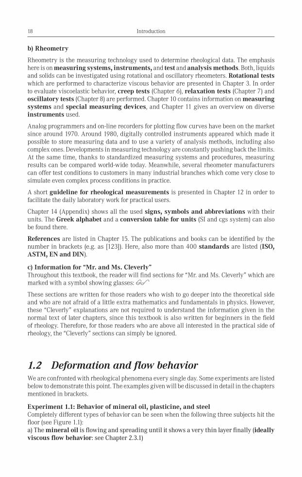
Experiment 1.1: Behavior of mineral oil, plasticine, and steelCompletely different types of behavior can be seen when the following three subjects hit the floor (see Figure 1.1):a) The mineral oil is flowing and spreading until it shows a very thin layer finally (ideally viscous flow behavior: see Chapter 2.3.1)
19Deformation and flow behavior
b) The plasticine will be deformed when it hits the floor, and afterwards, it remains deformed permanently (inhomogeneous plastic behavior outside the linear viscoelastic defor-mation range: see Chapter 3.3.4.3d)c) The steel ball bounces back, and exhibits afterwards no deformation at all (ideally elastic behavior: see Chapter 4.3.1)
Experiment 1.2: Playing with “bouncing putty” (some call it “Silly Putty”)The silicone polymer (unlinked PDMS) displays different rheological behaviors depen-ding on the period of time under stress (viscoelastic behavior of polymers: see Chapter 8.4, frequency sweep):a) When stressed briefly and quickly, the putty behaves like a rigid and elastic solid: If you mold a piece of it to the shape of a ball and throw it on the floor, it is bouncing back.b) When stressed slowly at a constantly low force over a longer period of time, the putty shows the behavior of a flexible and yielding, highly viscous liquid: If it is in the state of rest, thus, if you leave it untouched for a certain period of time, it is spreading very slowly under its own weight due to gravity to show an even layer with a homogeneous thickness finally.
Experiment 1.3: Do the rods remain in the position standing up straight?Three wooden rods are put into three glasses containing different materials and left for gra-vity to do its work. a) In the glass of water, the rod changes its position immediately and falls to the side of the glass (ideally viscous flow behavior: see Chapter 2.3.1). Additional observation: All the air bubbles which were brought into the water when immer-sing the rod are rising quickly within seconds.b) In the glass containing a silicone polymer (unlinked PDMS), the rod moves very, very slowly, reaching the side of the glass after around 10 minutes (polymers showing zero-shear viscosity: see Chapters 3.3.2.1a, 6.3.4.1 and 8.4.2.1a). Additional observation concerning the air bubbles which were brought into the polymer sample by the rod: Large bubbles are rising within a few minutes, but the smaller ones seem to remain suspended without visible motion. However, after several hours even the smallest bubble has reached the surface. Therefore, indeed long-term but complete de-aeration of the silicone occurs finally.c) In the glass containing a hand cream, the rod still remains standing straight in the initial position even after some hours (yield point: see Chapters 3.3.4 and 8.3.4.1; and structure strength at rest of dispersions: see Chapter 8.4.4a).Additional observation concerning the air bubbles: All bubbles, independent of their size, remain suspended, and therefore here, no de-aeration takes place at all.
SummaryRheological behavior depends on many influences. Above all, the following test conditions are important:• Typeofloading(presetofdeformation,velocityorforce;orshearstrain,shearrateorshear
stress, respectively) • Degreeofloading(low-shearorhigh-shearconditions)• Durationofloading(theperiodsoftimeunderloadandatrest)• Temperature(seeChapters3.5and8.6)
Figure 1.1: Deformation behavior after hitting the floor: a) mineral oil, b) plasticine, c) steel ball

Introduction20
Further important parameters are, for example:• Concentration(ofsolidparticlesinasuspension:seeChapter3.3.3;ofpolymermolecules
inasolution:seeChapter3.3.2.1a;ofsurfactantsinadispersion:seeChapter9).Usingan“Immobilization Cell,” the amount of liquid can be reduced under controlled conditions (e.g. when testing dispersions such as paper coatings: see Chapter 10.8.1.3).
• Ambientpressure(seeChapter3.6)• pHvalue(e.g.ofsurfactantsystems:seeChapter9).• Strengthofamagneticoranelectricfieldwheninvestigatingmagneto-rheologicalfluids
MRF or electro-rheological fluids ERF, respectively (see Chapters 10.8.1.1 and 2).• UVradiationcuring(e.g.ofresins,adhesivesandinks:seeChapter10.8.1.4).
21Definition of terms
Thomas G. Mezger: The Rheology Handbook© Copyright 2014 by Vincentz Network, Hanover, GermanyISBN 978-3-86630-650-9
2 Flow behavior and viscosity
In this chapter are explained the following terms given in bold:
2.1 IntroductionBefore 1980 in industrial practice, rheological experiments on pure liquids and dispersions were carried out almost exclusively in the form of rotational tests which enabled the characte-rization of flow behavior at medium and high flow velocities. Meanwhile since measurement technology has developed, many users have expanded their investigations on deformation and flow behavior performing measurements which cover also the low-shear range.
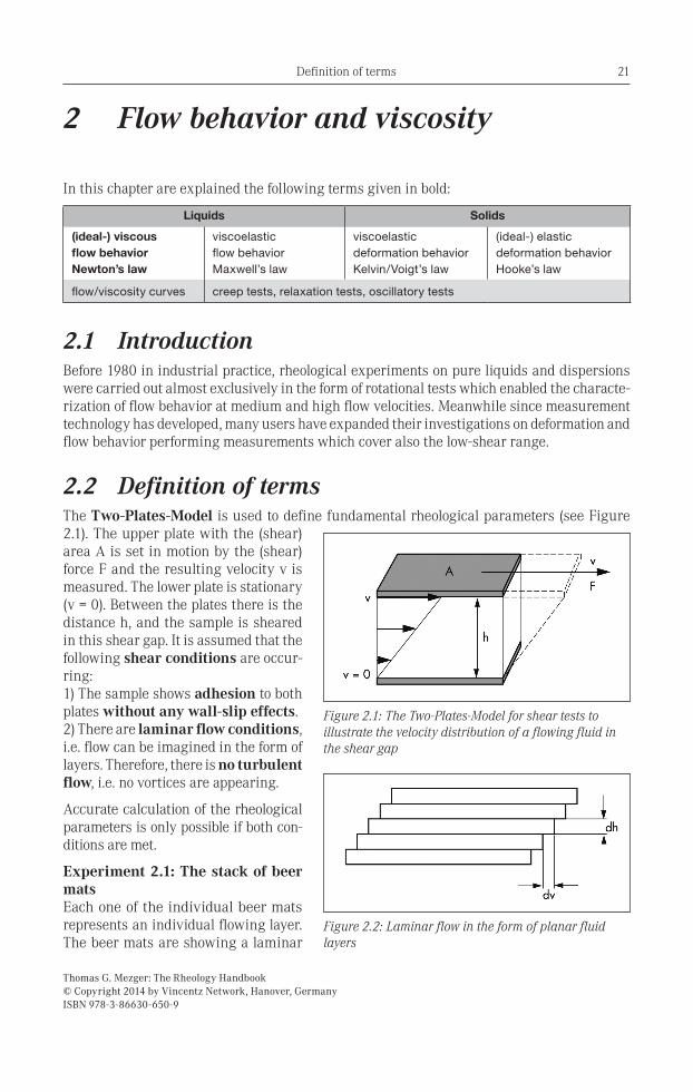
2.2 Definition of termsThe Two-Plates-Model is used to define fundamental rheological parameters (see Figure 2.1). The upper plate with the (shear) area A is set in motion by the (shear) force F and the resulting velocity v is measured. The lower plate is stationary (v = 0). Between the plates there is the distance h, and the sample is sheared in this shear gap. It is assumed that the following shear conditions are occur-ring:1) The sample shows adhesion to both plates without any wall-slip effects. 2) There are laminar flow conditions, i.e. flow can be imagined in the form of layers. Therefore, there is no turbulent flow, i.e. no vortices are appearing.
Accurate calculation of the rheological parameters is only possible if both con-ditions are met.
Experiment 2.1: The stack of beer matsEach one of the individual beer mats represents an individual flowing layer. The beer mats are showing a laminar
Liquids Solids
(ideal-) viscous flow behaviorNewton’s law
viscoelastic flow behavior Maxwell’s law
viscoelastic deformation behavior Kelvin/Voigt’s law
(ideal-) elastic deformation behavior Hooke’s law
flow/viscosity curves creep tests, relaxation tests, oscillatory tests
Figure 2.1: The Two-Plates-Model for shear tests to illustrate the velocity distribution of a flowing fluid in the shear gap
Figure 2.2: Laminar flow in the form of planar fluid layers
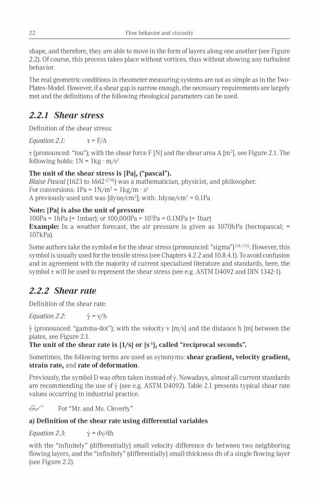
Flow behavior and viscosity22
shape, and therefore, they are able to move in the form of layers along one another (see Figure 2.2). Of course, this process takes place without vortices, thus without showing any turbulent behavior.
The real geometric conditions in rheometer measuring systems are not as simple as in the Two-Plates-Model. However, if a shear gap is narrow enough, the necessary requirements are largely met and the definitions of the following rheological parameters can be used.
2.2.1 Shear stressDefinition of the shear stress:
Equation 2.1: τ = F/A
τ (pronounced: “tou”); with the shear force F [N] and the shear area A [m2], see Figure 2.1. The following holds: 1N = 1kg · m/s2
The unit of the shear stress is [Pa], (“pascal”).Blaise Pascal (1623 to 1662 [278]) was a mathematician, physicist, and philosopher. For conversions: 1Pa = 1N/m2 = 1kg/m · s2
A previously used unit was [dyne/cm2]; with: 1dyne/cm2 = 0.1Pa
Note: [Pa] is also the unit of pressure100Pa = 1hPa (= 1mbar); or 100,000Pa = 105Pa = 0.1MPa (= 1bar)Example: In a weather forecast, the air pressure is given as 1070hPa (hectopascal; = 107kPa).
Some authors take the symbol σ for the shear stress (pronounced: “sigma”) [18, 215]. However, this symbol is usually used for the tensile stress (see Chapters 4.2.2 and 10.8.4.1). To avoid confusion and in agreement with the majority of current specialized literature and standards, here, the symbol τ will be used to represent the shear stress (see e.g. ASTM D4092 and DIN 1342-1).
2.2.2 Shear rateDefinition of the shear rate:
Equation 2.2: γ. = v/h
γ. (pronounced: “gamma-dot”); with the velocity v [m/s] and the distance h [m] between the
plates, see Figure 2.1.The unit of the shear rate is [1/s] or [s-1], called “reciprocal seconds”.
Sometimes, the following terms are used as synonyms: shear gradient, velocity gradient, strain rate, and rate of deformation.
Previously, the symbol D was often taken instead of γ.. Nowadays, almost all current standards
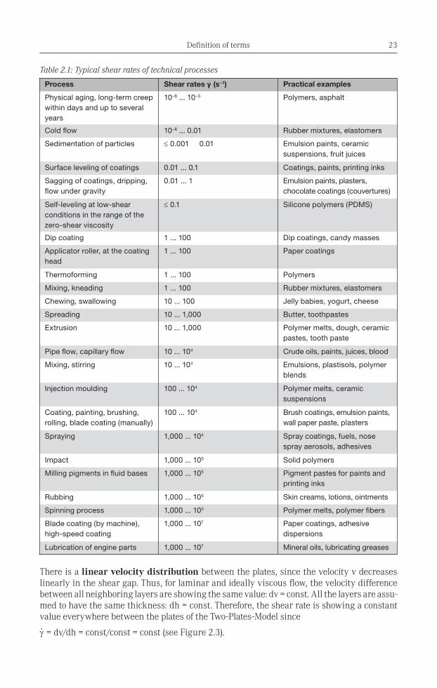
are recommending the use of γ. (see e.g. ASTM D4092). Table 2.1 presents typical shear rate
values occurring in industrial practice.
For “Mr. and Ms. Cleverly”
a) Definition of the shear rate using differential variables
Equation 2.3: γ. = dv/dh
with the “infinitely” (differentially) small velocity difference dv between two neighboring flowing layers, and the “infinitely” (differentially) small thickness dh of a single flowing layer (see Figure 2.2).
23Definition of terms
There is a linear velocity distribution between the plates, since the velocity v decreases linearly in the shear gap. Thus, for laminar and ideally viscous flow, the velocity difference between all neighboring layers are showing the same value: dv = const. All the layers are assu-med to have the same thickness: dh = const. Therefore, the shear rate is showing a constant value everywhere between the plates of the Two-Plates-Model since
γ. = dv/dh = const/const = const (see Figure 2.3).
Process Shear rates γ· (s–1) Practical examples
Physical aging, long-term creep within days and up to several years
10–8 ... 10–5 Polymers, asphalt
Cold flow 10–8 ... 0.01 Rubber mixtures, elastomers
Sedimentation of particles ≤ 0.001 0.01 Emulsion paints, ceramic suspensions, fruit juices
Surface leveling of coatings 0.01 ... 0.1 Coatings, paints, printing inks
Sagging of coatings, dripping, flow under gravity
0.01 ... 1 Emulsion paints, plasters, chocolate coatings (couvertures)
Self-leveling at low-shear conditions in the range of the zero-shear viscosity
≤ 0.1 Silicone polymers (PDMS)
Dip coating 1 ... 100 Dip coatings, candy masses
Applicator roller, at the coating head
1 ... 100 Paper coatings
Thermoforming 1 ... 100 Polymers
Mixing, kneading 1 ... 100 Rubber mixtures, elastomers
Chewing, swallowing 10 ... 100 Jelly babies, yogurt, cheese
Spreading 10 ... 1,000 Butter, toothpastes
Extrusion 10 ... 1,000 Polymer melts, dough, ceramic pastes, tooth paste
Pipe flow, capillary flow 10 ... 104 Crude oils, paints, juices, blood
Mixing, stirring 10 ... 104 Emulsions, plastisols, polymer blends
Injection moulding 100 ... 104 Polymer melts, ceramic suspensions
Coating, painting, brushing, rolling, blade coating (manually)
100 ... 104 Brush coatings, emulsion paints, wall paper paste, plasters
Spraying 1,000 ... 104 Spray coatings, fuels, nose spray aerosols, adhesives
Impact 1,000 ... 105 Solid polymers
Milling pigments in fluid bases 1,000 ... 105 Pigment pastes for paints and printing inks
Rubbing 1,000 ... 105 Skin creams, lotions, ointments
Spinning process 1,000 ... 105 Polymer melts, polymer fibers
Blade coating (by machine), high-speed coating
1,000 ... 107 Paper coatings, adhesive dispersions
Lubrication of engine parts 1,000 ... 107 Mineral oils, lubricating greases
Table 2.1: Typical shear rates of technical processes
Flow behavior and viscosity24
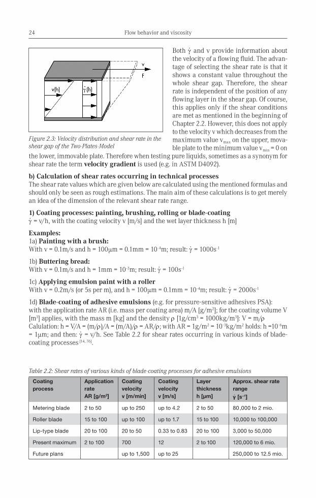
Both γ. and v provide information about
the velocity of a flowing fluid. The advan-tage of selecting the shear rate is that it shows a constant value throughout the whole shear gap. Therefore, the shear rate is independent of the position of any flowing layer in the shear gap. Of course, this applies only if the shear conditions are met as mentioned in the beginning of Chapter 2.2. However, this does not apply to the velocity v which decreases from the maximum value vmax on the upper, mova-ble plate to the minimum value vmin = 0 on
the lower, immovable plate. Therefore when testing pure liquids, sometimes as a synonym for shear rate the term velocity gradient is used (e.g. in ASTM D4092).
b) Calculation of shear rates occurring in technical processesThe shear rate values which are given below are calculated using the mentioned formulas and should only be seen as rough estimations. The main aim of these calculations is to get merely an idea of the dimension of the relevant shear rate range.
1) Coating processes: painting, brushing, rolling or blade-coating γ. = v/h, with the coating velocity v [m/s] and the wet layer thickness h [m]
Examples: 1a) Painting with a brush: With v = 0.1m/s and h = 100µm = 0.1mm = 10-4m; result: γ
. = 1000s-1
1b) Buttering bread: With v = 0.1m/s and h = 1mm = 10-3m; result: γ
. = 100s-1
1c) Applying emulsion paint with a rollerWith v = 0.2m/s (or 5s per m), and h = 100µm = 0.1mm = 10-4m; result: γ
. = 2000s-1
1d) Blade-coating of adhesive emulsions (e.g. for pressure-sensitive adhesives PSA): with the application rate AR (i.e. mass per coating area) m/A [g/m2]; for the coating volume V [m3] applies, with the mass m [kg] and the density ρ [1g/cm3 = 1000kg/m3]: V = m/ρCalulation: h = V/A = (m/ρ)/A = (m/A)/ρ = AR/ρ; with AR = 1g/m2 = 10-3kg/m2 holds: h =10-6m = 1µm; and then: γ
. = v/h. See Table 2.2 for shear rates occurring in various kinds of blade-
coating processes [14, 76].
Figure 2.3: Velocity distribution and shear rate in the shear gap of the Two-Plates-Model
Coating process
Application rate AR [g/m2]
Coating velocity v [m/min]
Coating velocity v [m/s]
Layer thickness h [µm]
Approx. shear rate range
γ· [s–1]
Metering blade 2 to 50 up to 250 up to 4.2 2 to 50 80,000 to 2 mio.
Roller blade 15 to 100 up to 100 up to 1.7 15 to 100 10,000 to 100,000
Lip-type blade 20 to 100 20 to 50 0.33 to 0.83 20 to 100 3,000 to 50,000
Present maximum 2 to 100 700 12 2 to 100 120,000 to 6 mio.
Future plans up to 1,500 up to 25 250,000 to 12.5 mio.
Table 2.2: Shear rates of various kinds of blade-coating processes for adhesive emulsions
25Definition of terms
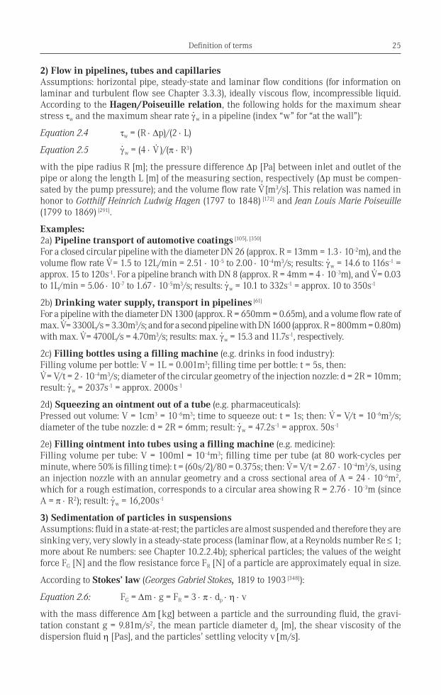
2) Flow in pipelines, tubes and capillariesAssumptions: horizontal pipe, steady-state and laminar flow conditions (for information on laminar and turbulent flow see Chapter 3.3.3), ideally viscous flow, incompressible liquid. According to the Hagen/Poiseuille relation, the following holds for the maximum shear stress τw and the maximum shear rate γ
.w in a pipeline (index “w” for “at the wall”):
Equation 2.4 τw = (R ⋅ ∆p)/(2 ⋅ L)
Equation 2.5 γ.
w = (4 ⋅ V. )/(π ⋅ R3)
with the pipe radius R [m]; the pressure difference ∆p [Pa] between inlet and outlet of the pipe or along the length L [m] of the measuring section, respectively (∆p must be compen-sated by the pump pressure); and the volume flow rate V
. [m3/s]. This relation was named in
honor to Gotthilf Heinrich Ludwig Hagen (1797 to 1848) [172] and Jean Louis Marie Poiseuille (1799 to 1869) [291].
Examples:2a) Pipeline transport of automotive coatings [105], [350]
For a closed circular pipeline with the diameter DN 26 (approx. R = 13mm = 1.3 ⋅ 10-2m), and the volume flow rate V
. = 1.5 to 12L/min = 2.51 ⋅ 10-5 to 2.00 ⋅ 10-4m3/s; results: γ
.w = 14.6 to 116s-1 =
approx. 15 to 120s-1. For a pipeline branch with DN 8 (approx. R = 4mm = 4 ⋅ 10-3m), and V. = 0.03
to 1L/min = 5.06 ⋅ 10-7 to 1.67 ⋅ 10-5m3/s; results: γ.
w = 10.1 to 332s-1 = approx. 10 to 350s-1
2b) Drinking water supply, transport in pipelines [61]
For a pipeline with the diameter DN 1300 (approx. R = 650mm = 0.65m), and a volume flow rate of max. V
. = 3300L/s = 3.30m3/s; and for a second pipeline with DN 1600 (approx. R = 800mm = 0.80m)
with max. V. = 4700L/s = 4.70m3/s; results: max. γ
.w = 15.3 and 11.7s-1, respectively.
2c) Filling bottles using a filling machine (e.g. drinks in food industry):Filling volume per bottle: V = 1L = 0.001m3; filling time per bottle: t = 5s, then: V. = V/t = 2 ⋅ 10-4m3/s; diameter of the circular geometry of the injection nozzle: d = 2R = 10mm;
result: γ.
w = 2037s-1 = approx. 2000s-1
2d) Squeezing an ointment out of a tube (e.g. pharmaceuticals):Pressed out volume: V = 1cm3 = 10-6m3; time to squeeze out: t = 1s; then: V
. = V/t = 10-6m3/s;
diameter of the tube nozzle: d = 2R = 6mm; result: γ.
w = 47.2s-1 = approx. 50s-1
2e) Filling ointment into tubes using a filling machine (e.g. medicine): Filling volume per tube: V = 100ml = 10-4m3; filling time per tube (at 80 work-cycles per minute, where 50% is filling time): t = (60s/2)/80 = 0.375s; then: V
. = V/t = 2.67 ⋅ 10-4m3/s, using
an injection nozzle with an annular geometry and a cross sectional area of A = 24 ⋅ 10-6m2, which for a rough estimation, corresponds to a circular area showing R = 2.76 ⋅ 10-3m (since A = π ⋅ R2); result: γ
.w = 16,200s-1
3) Sedimentation of particles in suspensionsAssumptions: fluid in a state-at-rest; the particles are almost suspended and therefore they are sinking very, very slowly in a steady-state process (laminar flow, at a Reynolds number Re ≤ 1; more about Re numbers: see Chapter 10.2.2.4b); spherical particles; the values of the weight force FG [N] and the flow resistance force FR [N] of a particle are approximately equal in size.
According to Stokes’ law (Georges Gabriel Stokes, 1819 to 1903 [348]):
Equation 2.6: FG = ∆m ⋅ g = FR = 3 ⋅ π ⋅ dp ⋅ η ⋅ v
with the mass difference ∆m [kg] between a particle and the surrounding fluid, the gravi-tation constant g = 9.81m/s2, the mean particle diameter dp [m], the shear viscosity of the dispersion fluid η [Pas], and the particles’ settling velocity v [m/s].
Flow behavior and viscosity26
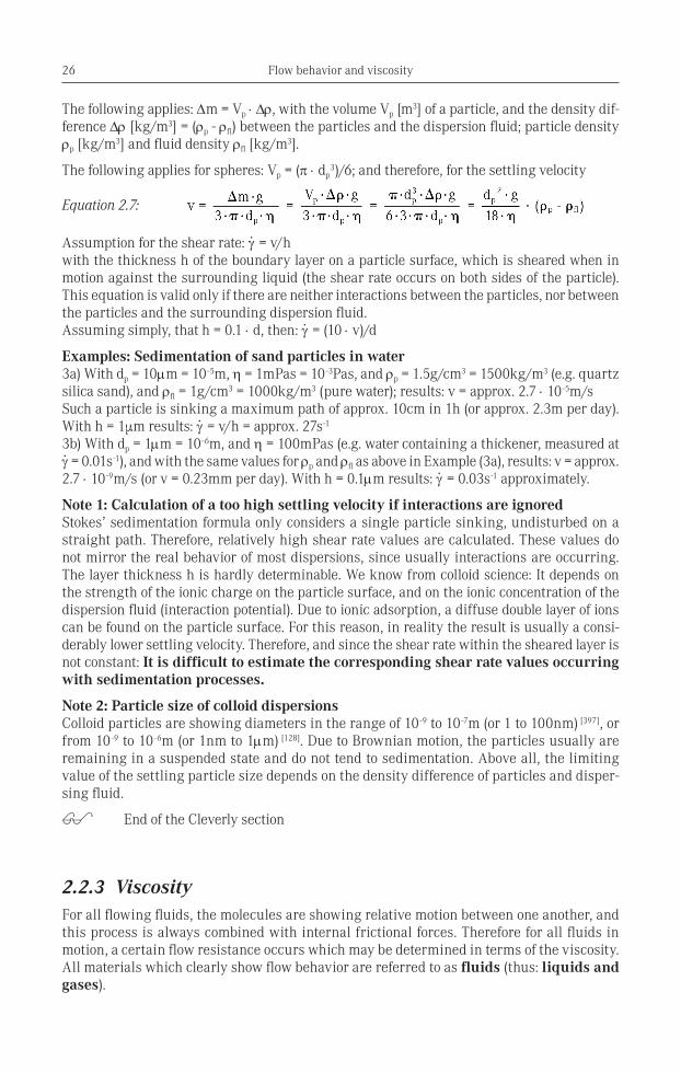
The following applies: ∆m = Vp ⋅ ∆ρ, with the volume Vp [m3] of a particle, and the density dif-ference ∆ρ [kg/m3] = (ρp - ρfl) between the particles and the dispersion fluid; particle density ρp [kg/m3] and fluid density ρfl [kg/m3].
The following applies for spheres: Vp = (π ⋅ dp3)/6; and therefore, for the settling velocity
Equation 2.7:
Assumption for the shear rate: γ. = v/h
with the thickness h of the boundary layer on a particle surface, which is sheared when in motion against the surrounding liquid (the shear rate occurs on both sides of the particle). This equation is valid only if there are neither interactions between the particles, nor between the particles and the surrounding dispersion fluid. Assuming simply, that h = 0.1 ⋅ d, then: γ
. = (10 ⋅ v)/d
Examples: Sedimentation of sand particles in water3a) With dp = 10µm = 10-5m, η = 1mPas = 10-3Pas, and ρp = 1.5g/cm3 = 1500kg/m3 (e.g. quartz silica sand), and ρfl = 1g/cm3 = 1000kg/m3 (pure water); results: v = approx. 2.7 ⋅ 10-5m/sSuch a particle is sinking a maximum path of approx. 10cm in 1h (or approx. 2.3m per day). With h = 1µm results: γ
. = v/h = approx. 27s-1
3b) With dp = 1µm = 10-6m, and η = 100mPas (e.g. water containing a thickener, measured at γ. = 0.01s-1), and with the same values for ρp and ρfl as above in Example (3a), results: v = approx.
2.7 ⋅ 10-9m/s (or v = 0.23mm per day). With h = 0.1µm results: γ. = 0.03s-1 approximately.
Note 1: Calculation of a too high settling velocity if interactions are ignoredStokes’ sedimentation formula only considers a single particle sinking, undisturbed on a straight path. Therefore, relatively high shear rate values are calculated. These values do not mirror the real behavior of most dispersions, since usually interactions are occurring. The layer thickness h is hardly determinable. We know from colloid science: It depends on the strength of the ionic charge on the particle surface, and on the ionic concentration of the dispersion fluid (interaction potential). Due to ionic adsorption, a diffuse double layer of ions can be found on the particle surface. For this reason, in reality the result is usually a consi-derably lower settling velocity. Therefore, and since the shear rate within the sheared layer is not constant: It is difficult to estimate the corresponding shear rate values occurring with sedimentation processes.
Note 2: Particle size of colloid dispersionsColloid particles are showing diameters in the range of 10-9 to 10-7m (or 1 to 100nm) [397], or from 10-9 to 10-6m (or 1nm to 1µm) [128]. Due to Brownian motion, the particles usually are remaining in a suspended state and do not tend to sedimentation. Above all, the limiting value of the settling particle size depends on the density difference of particles and disper-sing fluid.
End of the Cleverly section
2.2.3 ViscosityFor all flowing fluids, the molecules are showing relative motion between one another, and this process is always combined with internal frictional forces. Therefore for all fluids in motion, a certain flow resistance occurs which may be determined in terms of the viscosity. All materials which clearly show flow behavior are referred to as fluids (thus: liquids and gases).
27Definition of terms
a) Shear viscosityFor ideally viscous fluids measured at a constant temperature, the value of the ratio of shear stress τ and corresponding shear rate γ
. is a material constant. Definition of the shear
viscosity:
Equation 2.8: η = τ/γ.
η (eta, pronounced: “etah” or “atah”), the unit of shear viscosity is [Pas], (“pascal-seconds“).
The following holds: 1Pas = 1N ⋅ s/m2 = 1kg/s ⋅ m
For low-viscosity liquids, the following unit is usually used:1mPas (“milli-pascal-seconds”) = 10-3PasSometimes, for highly viscous samples the following units are used:1kPas (“kilo-pascal-seconds”) = 1000Pas = 103Pas, or even 1MPas (“mega-pascal-seconds”) = 1,000kPas = 1,000,000Pas = 106PasA previously used unit was [P], (“poise”; at best pronounced in French); and: 1P = 100cP; however, this is not an SI unit [59]. This unit was named in honor to the doctor and physicist Jean L.M. Poiseuille (1799 to 1869) [291]. The following holds: 1cP (“centi-poise”) = 1mPas, and 1P = 0.1Pas = 100mPas
Sometimes, the term “dynamic viscosity” is used for η (as in DIN 1342-1). However, some people use the same term to describe either the complex viscosity determined by oscillatory tests, or to mean just the real part of the complex viscosity (the two terms are explained in Chapter 8.2.4b). To avoid confusion and in agreement with the majority of current internati-onal authors, here, the term “viscosity” or “shear viscosity” will be used for η. Table 2.3 lists viscosity values of various materials.
The inverse value of viscosity is referred to as fluidity ϕ (phi, pronounced: “fee” or “fi”) [303]. However today, this parameter is rarely used. The following holds:
Equation 2.9: ϕ = 1/η with the unit [1/Pas] = [Pas-1]
For “Mr. and Ms. Cleverly”
Note 1: Usually, samples are viscoelastic when showing high viscosity values.Many rheological investigations showed that at values of η > 10kPas, the elastic portion should no longer be ignored. These kinds of samples should no longer be considered simply viscous only, but visco-elastic (see also Chapter 5).
Note 2: Shear viscosity η and extensional viscosity ηE For ideally viscous fluids under uniaxial tension the following applies for the values of the extensional viscosity (in Pas) and shear viscosity η (also in Pas): ηE(ε
.) = 3 ⋅ η(γ
.), if the values
of the extensional strain rate ε. [s-1] and shear rate γ
. [s-1] are equal in size (see also Chapter
10.8.4.1: Trouton relation).
End of the Cleverly section
b) Kinematic viscosityDefinition of the kinematic viscosity:
Equation 2.10: ν = η/ρ
ν (ny, pronounced: “nu” or “new”), with the density ρ [kg/m3], (rho, pronounced: “ro”).For the unit of density holds: 1g/cm3 = 1000kg/m3
The unit of kinematic viscosity is [mm2/s]; and: 1mm2/s = 10-6m2/s
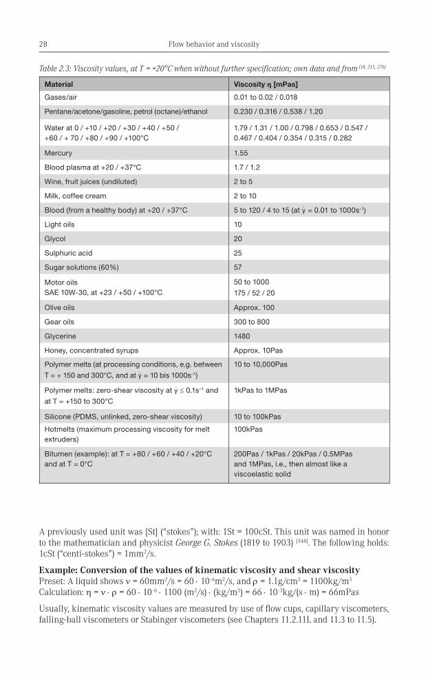
Flow behavior and viscosity28
A previously used unit was [St] (“stokes”); with: 1St = 100cSt. This unit was named in honor to the mathematician and physicist George G. Stokes (1819 to 1903) [348]. The following holds: 1cSt (“centi-stokes”) = 1mm2/s.
Example: Conversion of the values of kinematic viscosity and shear viscosity Preset: A liquid shows ν = 60mm2/s = 60 ⋅ 10-6m2/s, and ρ = 1.1g/cm3 = 1100kg/m3
Calculation: η = ν ⋅ ρ = 60 ⋅ 10-6 ⋅ 1100 (m2/s) ⋅ (kg/m3) = 66 ⋅ 10-3kg/(s ⋅ m) = 66mPas
Usually, kinematic viscosity values are measured by use of flow cups, capillary viscometers, falling-ball viscometers or Stabinger viscometers (see Chapters 11.2.11L and 11.3 to 11.5).
Material Viscosity η [mPas]
Gases/air 0.01 to 0.02 / 0.018
Pentane/acetone/gasoline, petrol (octane)/ethanol 0.230 / 0.316 / 0.538 / 1.20
Water at 0 / +10 / +20 / +30 / +40 / +50 / +60 / + 70 / +80 / +90 / +100°C
1.79 / 1.31 / 1.00 / 0.798 / 0.653 / 0.547 / 0.467 / 0.404 / 0.354 / 0.315 / 0.282
Mercury 1.55
Blood plasma at +20 / +37°C 1.7 / 1.2
Wine, fruit juices (undiluted) 2 to 5
Milk, coffee cream 2 to 10
Blood (from a healthy body) at +20 / +37°C 5 to 120 / 4 to 15 (at γ· = 0.01 to 1000s–1)
Light oils 10
Glycol 20
Sulphuric acid 25
Sugar solutions (60%) 57
Motor oils SAE 10W-30, at +23 / +50 / +100°C
50 to 1000
175 / 52 / 20
Olive oils Approx. 100
Gear oils 300 to 800
Glycerine 1480
Honey, concentrated syrups Approx. 10Pas
Polymer melts (at processing conditions, e.g. between
T = + 150 and 300°C, and at γ· = 10 bis 1000s–1)
10 to 10,000Pas
Polymer melts: zero-shear viscosity at γ· ≤ 0.1s–1 and
at T = +150 to 300°C
1kPas to 1MPas
Silicone (PDMS, unlinked, zero-shear viscosity) 10 to 100kPas
Hotmelts (maximum processing viscosity for melt extruders)
100kPas
Bitumen (example): at T = +80 / +60 / +40 / +20°C and at T = 0°C
200Pas / 1kPas / 20kPas / 0.5MPas and 1MPas, i.e., then almost like a viscoelastic solid
Table 2.3: Viscosity values, at T = +20°C when without further specification; own data and from [18, 215, 276]
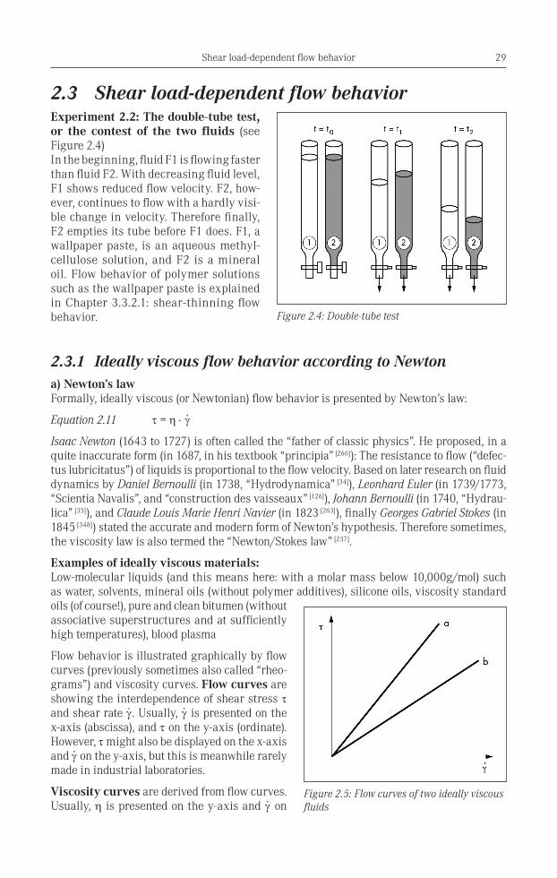
29Shear load-dependent flow behavior
2.3 Shear load-dependent flow behavior Experiment 2.2: The double-tube test, or the contest of the two fluids (see Figure 2.4)In the beginning, fluid F1 is flowing faster than fluid F2. With decreasing fluid level, F1 shows reduced flow velocity. F2, how-ever, continues to flow with a hardly visi-ble change in velocity. Therefore finally, F2 empties its tube before F1 does. F1, a wallpaper paste, is an aqueous methyl-cellulose solution, and F2 is a mineral oil. Flow behavior of polymer solutions such as the wallpaper paste is explained in Chapter 3.3.2.1: shear-thinning flow behavior.
2.3.1 Ideally viscous flow behavior according to Newtona) Newton’s lawFormally, ideally viscous (or Newtonian) flow behavior is presented by Newton’s law:
Equation 2.11 τ = η ⋅ γ.
Isaac Newton (1643 to 1727) is often called the “father of classic physics”. He proposed, in a quite inaccurate form (in 1687, in his textbook “principia” [266]): The resistance to flow (“defec-tus lubricitatus”) of liquids is proportional to the flow velocity. Based on later research on fluid dynamics by Daniel Bernoulli (in 1738, “Hydrodynamica” [34]), Leonhard Euler (in 1739/1773, “Scientia Navalis”, and “construction des vaisseaux” [126]), Johann Bernoulli (in 1740, “Hydrau-lica” [35]), and Claude Louis Marie Henri Navier (in 1823 [263]), finally Georges Gabriel Stokes (in 1845 [348]) stated the accurate and modern form of Newton’s hypothesis. Therefore sometimes, the viscosity law is also termed the “Newton/Stokes law” [237].
Examples of ideally viscous materials:Low-molecular liquids (and this means here: with a molar mass below 10,000g/mol) such as water, solvents, mineral oils (without polymer additives), silicone oils, viscosity standard oils (of course!), pure and clean bitumen (without associative superstructures and at sufficiently high temperatures), blood plasma
Flow behavior is illustrated graphically by flow curves (previously sometimes also called “rheo-grams”) and viscosity curves. Flow curves are showing the interdependence of shear stress τ and shear rate γ
.. Usually, γ
. is presented on the
x-axis (abscissa), and τ on the y-axis (ordinate). However, τ might also be displayed on the x-axis and γ
. on the y-axis, but this is meanwhile rarely
made in industrial laboratories.
Viscosity curves are derived from flow curves. Usually, η is presented on the y-axis and γ
. on
Figure 2.4: Double-tube test
Figure 2.5: Flow curves of two ideally viscous fluids