This page intentionally left blank

Topology and Its Applications

PURE AND APPLIED MATHEMATICS

A Wiley-Interscience Series of Texts, Monographs, and Tracts

Founded by RICHARD COURANT Editors Emeriti: MYRON B. ALLEN III, DAVID A. COX, PETER HILTON, HARRY HOCHSTADT, PETER LAX, JOHN TOLAND

A complete list of the titles in this series appears at the end of this volume.

Topology and Its Applications

iam F. Basener Rochester Institute of Technology

Department of Mathematics and Statistics Rochester, NY

WILEY-INTERSCIENCE

A JOHN WILEY & SONS, INC., PUBLICATION

This material is based upon work supported by the National Science Foundation under Grant No. DUE 0442740. Any opinions, findings, and conclusions or recommendations expressed in this material are those of the author(s) and do not necessarily reflect the views of the National Science Foundation.

Copyright © 2006 by John Wiley & Sons, Inc. All rights reserved.

Published by John Wiley & Sons, Inc., Hoboken, New Jersey. Published simultaneously in Canada.

No part of this publication may be reproduced, stored in a retrieval system, or transmitted in any form or by any means, electronic, mechanical, photocopying, recording, scanning, or otherwise, except as permitted under Section 107 or 108 of the 1976 United States Copyright Act, without either the prior written permission of the Publisher, or authorization through payment of the appropriate per-copy fee to the Copyright Clearance Center, Inc., 222 Rosewood Drive, Danvers, MA 01923, (978) 750-8400, fax (978) 750-4470, or on the web at www.copyright.com. Requests to the Publisher for permission should be addressed to the Permissions Department, John Wiley & Sons, Inc., 111 River Street, Hoboken, NJ 07030, (201) 748-6011, fax (201) 748-6008, or online at http://www.wiley.com/go/permission.

Limit of Liability/Disclaimer of Warranty: While the publisher and author have used their best efforts in preparing this book, they make no representations or warranties with respect to the accuracy or completeness of the contents of this book and specifically disclaim any implied warranties of merchantability or fitness for a particular purpose. No warranty may be created or extended by sales representatives or written sales materials. The advice and strategies contained herein may not be suitable for your situation. You should consult with a professional where appropriate. Neither the publisher nor author shall be liable for any loss of profit or any other commercial damages, including but not limited to special, incidental, consequential, or other damages.

For general information on our other products and services or for technical support, please contact our Customer Care Department within the United States at (800) 762-2974, outside the United States at (317) 572-3993 or fax (317) 572-4002.

Wiley also publishes its books in a variety of electronic formats. Some content that appears in print may not be available in electronic format. For information about Wiley products, visit our web site at www.wiley.com.

Library of Congress Cataloging-in-Publication Data:

Basener, William F., 1973 Topology and its applications / William F. Basener.

p. cm. Includes bibliographical references and index. ISBN-13 978-0-471-68755-9 ISBN-10 0-471-68755-3 (cloth; alk. paper) 1. Topology—Textbooks. I. Title.

QA611.B275 2006 514—dc22 2006046178

Printed in the United States of America.

10 9 8 7 6 5 4 3

To my wonderful wife, Amber, without whose support this endeavor would have been impossible.

And to our beautiful children, Abigail, Wesley, Lila and J. T.

"The heavens tell of the glory of God. The skies display his marvelous craftsmanship"

Psalm 19:1

This page intentionally left blank

Contents

Preface xxv

Introduction xxix 1.1 Preliminaries xxxii 1.2 Cardinality xxxv

1 Continuity 1 1.1 Continuity and Open Sets in Rn 1 1.2 Continuity and Open Sets in Topological Spaces 6 1.3 Metric, Product, and Quotient Topologies 9 1.4 Subsets of Topological Spaces 19 1.5 Continuous Functions and Topological Equivalence 27 1.6 Surfaces 34 1.7 Application: Chaos in Dynamical Systems 39

1.7.1 History of Chaos 39 1.7.2 A Simple Example 40 1.7.3 Notions of Chaos 41

2 Compactness and Connectedness 47 2.1 Closed Bounded Subsets ofR 47 2.2 Compact Spaces 51

Vl l

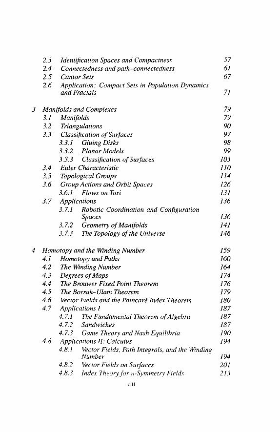
2.3 Identification Spaces and Compactness 57 2.4 Connectedness and path-connectedness 61 2.5 Cantor Sets 67 2.6 Application: Compact Sets in Population Dynamics

and Fractals 71

3 Manifolds and Complexes 79 3.1 Manifolds 79 3.2 Triangulations 90 3.3 Classification of Surfaces 97

3.3.1 Gluing Disks 98 3.3.2 Planar Models 99 3.3.3 Classification of Surfaces 103

3.4 Euler Characteristic 110 3.5 Topological Groups 114 3.6 Group Actions and Orbit Spaces 126

3.6.1 Flows on Tori 131 3.7 Applications 136

3.7.1 Robotic Coordination and Configuration Spaces 136

3.7.2 Geometry of Manifolds 141 3.7.3 The Topology of the Universe 146

4 Homotopy and the Winding Number 159 4.1 Homotopy and Paths 160 4.2 The Winding Number 164 4.3 Degrees of Maps 174 4.4 The Brouwer Fixed Point Theorem 176 4.5 The Borsuk-Ulam Theorem 179 4.6 Vector Fields and the Poincare Index Theorem 180 4.7 Applications I 187

4.7.1 The Fundamental Theorem of Algebra 187 4.7.2 Sandwiches 187 4.7.3 Game Theory and Nash Equilibria 190

4.8 Applications II: Calculus 194 4.8.1 Vector Fields, Path Integrals, and the Winding

Number 194 4.8.2 Vector Fields on Surfaces 201 4.8.3 Index Theory for n-Symmetry Fields 213

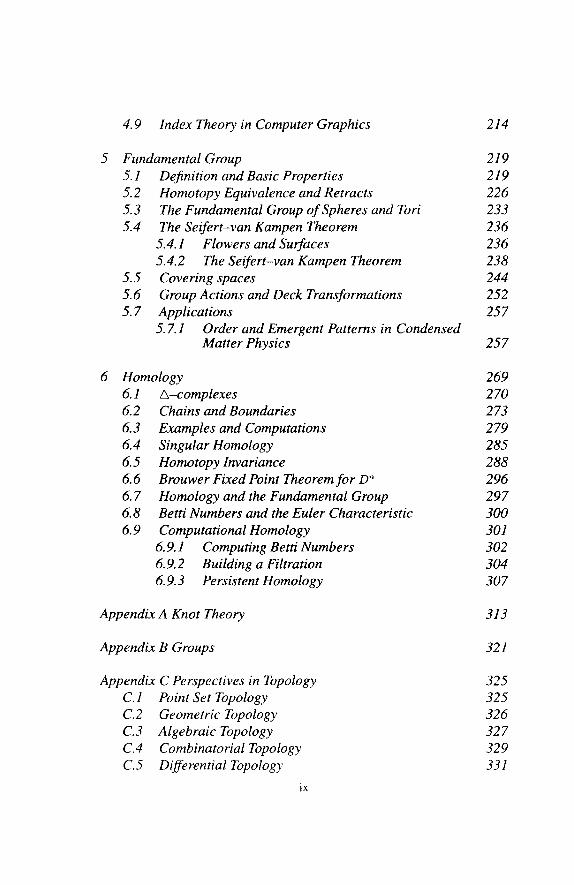
4.9 Index Theory in Computer Graphics 214

Fundamental Group 5.1 5.2 5.3 5.4

5.5 5.6 5.7

Definition and Basic Properties Homotopy Equivalence and Retracts The Fundamental Group of Spheres and Tori The Seifert-van Kampen Theorem

5.4.1 Flowers and Surfaces 5.4.2 The Seifert-van Kampen Theorem Covering spaces Group Actions and Deck Transformations Applications 5.7.1 Order and Emergent Patterns in Condensed

Matter Physics

Homology 6.1 6.2 6.3 6.4 6.5 6.6 6.7 6.8 6.9

/^-complexes Chains and Boundaries Examples and Computations Singular Homology Homotopy Invariance Brouwer Fixed Point Theorem for Dn

Homology and the Fundamental Group Betti Numbers and the Euler Characteristic Computational Homology

6.9.1 Computing Betti Numbers 6.9.2 Building a Filtration 6.9.3 Persistent Homology

219 219 226 233 236 236 238 244 252 257

257

269 270 273 279 285 288 296 297 300 301 302 304 307

Appendix A Knot Theory 313

Appendix B Groups 321

Appendix C Perspectives in Topology 325 C.l Point Set Topology 325 C.2 Geometric Topology 326 C.3 Algebraic Topology 327 C.4 Combinatorial Topology 329 C.5 Differential Topology 331

IX

References 333

Bibliography 333

Index 337

List of Figures

LI Cantor's diagonalization argument. xxxvii

LI The graph of a function f that is continuous and a function g that is not continuous. 2

1.2 The definition of continuity using balls. 4

1.3 The open balls from the proof of Proposition 6. 5

1.4 The function f is continuous and the function g is not continuous. 6

1.5 The functions f and h are close in the άλ metric but not in the d0 metric. 11

1.6 The product of a circle and an interval. 13

1.7 The 2-dimensional torus T2 = C x C. The vertical circles shown in the torus are subsets of the form {x} x C. Horizontal circles are subsets of the form C x {x}. 14

1.8 Making a Mobius strip by identifying edges of a square. 15

L9 Making a torus by identifying edges of a square. 16

1.10 Making a Klein bottle by identifying edges of a square. 16

1.11 The dunce cap. All three vertices are identified together. 19

1.12 The topologist's sine curve {(x, sin(l/a;)) \x > 0}. 21

1.13 A circle is topologically equivalent to the outline of a duckf but not to the number eight or to a circle with a line. 30

1.14 The stereographic projection π : Sn - NP —> Rn. 31

1.15 An open set in C whose image under f is not open. 33

1.16 A surface locally resembles the plane. 35

1.17 The process of forming the connected sum of two tori to make M2. 36

1.18 The classification of surfaces. 3 7

1.19 The projective plane is a Mobius strip with a disk identified along their boundary circles. 38

1.20 An identification on the unit square that results in the projective plane. 38

1.21 The sets from the proof of Theorem 12. 44

2.1 A compact surface with finitely many holes and a noncompact surface with infinitely many holes. The noncompact surface repeats infinitely in both directions 50

2.2 The sets used in the proof of Theorem 20. 53

2.3 The sets used in the proof of Theorem 24. 56

2.4 The Hawaiian earring. 60

2.5 The intermediate value theorem. 63

2.6 A space that is path-connected and locally connected but not locally path-connected. 66

2.7 The middle-thirds Cantor set as the intersection of an infinite sequence of sets. 69

2.8 The third step in the construction ofAntoine's necklace. 70

2.9 The Sierpinski gasket. 71

2.10 The discrete logistic function with k = 2, k = 4, and k = 6. 72

2.11 The Cantor set as the set of initial conditions for populations that do not leave the interval [0,1]. 73

2.12 The compact positively invariant sets for F with a = 0.3, c = 3, and h = 1.5335. 75

2.13 The compact positively invariant sets for F with a = 1, c = 3.5, and h = 1.275. 76

2.14 Two different filled Julia sets. The upper filled Julia set was generated using the parameter c = -0.615 + 0.4i The lower one was generated using the parameter c = -0.621 + OAi. 77

2.15 The Mandelbrot set. 78 3.1 A chart in a manifold. 80 3.2 Charts in manifolds with boundary. 81 3.3 A map f : R+ -* R2 and a map g : C -* R2. Both maps

are immersions but not embeddings. 82 3.4 Traveling around a nonorientable manifold can

reverse left-and righthandedness. 83

3.5 A chart satisfying Bx (0) c φ'α (Ua) c B2 (0). 85 3.6 The Mobius strip and the Klein Bottle as fiber bundles. 87 3.7 The identification resulting in the Poincare

dodecahedral space. 88 3.8 k-simplexes. 91 3.9 Two 2-dimensional simplicial complexes. The

complex on the right is topologically a sphere. The shading indicates triangles that are included in the complex. 91

3.10 Intersections between triangles that are not permitted in a triangulation. 92

3.11 A triangulation of the sphere. 92 3.12 Triangulations of the torus and the projective plane. 92 3.13 Triangulations meeting at a point in a triangulation

of a surface. 93 3.14 Permitted intersections between disks and a forbidden

intersection between disks. 94

3.15 Making a triangulationfrom the cover by compact disks. 94

3.16 Orientations on simplexes. 95

3.17 Orientations of the first two triangles are not compatible, while orientations of the second pair of triangles are compatible. 96

3.18 Gluing two disks along a pair of arcs. 98

3.19 Building a torus as a cell complex. 100

3.20 Simple planar models for familiar surfaces. 101

3.21 A planar model for the 2-holed torus. 101

3.22 Triangulations of the planar models aa and aa~l. 102

3.23 The first planar model is orientable, while the second

is not. 103

3.24 A cross cap. 104

3.25 Building a planar mode I for the connected sum of two tori. 105

3.26 The cancellation rule Axx~lB ~ AB. 106 3.27 The cylinder cut-and-paste rule ABxCDx~l ~

BAxDCx~\ 107

3.28 The classification of surfaces. 108

3.29 Reducing the number of vertices in P. 109

3.30 A tetrahedron, a cube, a cube with a hole drilled out, a 2-simplex, a graph with no loops, and a graph with two loops. Ill

3.31 A loop in the 3-sphere in M corresponds to two full rotations. Both 3-manifolds are depicted using their 2-dimensional counterparts. 123

3.32 Orbits under the group actions from Examples 1 through 5. 127

3.33 The flow defined by </>(£, (#,?/)) = (xet,ye~t). Also shown is the vector field for the differential equation x' = x,y' — —y. 128

3.34 The Hopf bundle on the 3-sphere S3 c R4. The Hopf link is shown in bold. One circle in this link is shown as a vertical line through infinity. 130

xiv

3.35 The constant slope flow on a 2-torus. 132

3.36 The configuration space C2 with the diagonal shown as a dotted line. The faint dashed line is the self-intersection forced from the immersion in three dimensions. The path 7 from (A,B) to (B,A) is also shown. 137

3.37 The configuration space C2(T) cut open along the diagonal is shown in the lefthand diagram. The righthand diagram shows the discretization ofC2(T). 138

3.38 The graph Q, its configuration space, and the discretized configuration space. 139

3.39 The graph X, its configuration space, and the discretized configuration space. 139

3.40 The graphs K5 (lefi) and #3,3 (right). The notation for these graphs comes from graph theory. 140

3.41 Geodesies in the Poincare disk model for the hyperbolic plane. Diagram (a) shows a family of geodesies that meet dD at the same point. Diagram (b) shows a geodesic, which is the horizontal diameter of D, together with a family of orthogonal geodesies. Diagram (c) shows two octagons in H2. Larger octagons will have smaller interior angles. 143

3.42 Diagram (a) shows the tiling of H2 by octagons. Diagram (b) shows an initial "large" octagon, and a neighboring one obtained by reflecting in L and then M. 144

3.43 The three possible geometries on surfaces. 145

3.44 A person living in a spherical universe: (a) the physical universe; (b) the universe as it appears to an observer. 147

3.45 A person living in a 2-torus: (a) the physical universe; (b) the universe as it appears to an observer. The ponytail indicates the direction in which each image is facing. 148

3.46 A person living in a Klein bottle: (a) the physical universe (b) the universe as it appears to an observer. The ponytail indicates the direction in which each image is facing. 148

XV

3.47 A person living in a 2-holed torus. The ponytail indicates the direction in which each image is facing. 149

3.48 A Poincare dodecahedral universe as seen from the inside. (Figure courtesy of Jeff Weeks.) 150

3.49 NASA missions for seeing very old light. (Figure courtesy of the NASA/WMAP Science Team.) 152

3.50 The WMAP data for the cosmic microwave background radiation. (Figure courtesy of the NASA/WMAP Science Team.) 152

3.51 Part (a) shows a collection of galactic clusters. Part (b) shows the same collections of clusters with the most frequently occurring distances highlighted, suggesting that this universe is a torus. 154

3.52 Part (a) shows a PSHfor a universe which would not result in multiple self-images, such as R3 or S3. Part (b) shows a PSHfor a 3-torus. 155

3.53 The photons now arriving at Earth in the form of CMB radiation all began their journeys on the last scattering surface. 155

3.54 The types of pairs of matching circles that might exist in the CMB if the universe were a 3-torus. 156

4.1 Two loops a and β in R2 - P that are not base point homotopic. 161

4.2 An end point preserving homotopy from the path 70 to the path 71. 161

4.3 The homotopy of the identity map of a disk to a constant map. 163

4.4 The covering maps pi : {(x,y,n) € R3|(x,y) € R2, and n e N} -> R2 and p2 : R -+ C from Examples 2 and 3. For the map p2, the real line R is shown as a helix sitting above C. 166

4.5 The lift of a path in R2 - P. 167 4.6 Value ofW{^, P)for P in each of the components of

R2-Im(7). 170 4.7 The curve from Figure 4.6 filled using the nonzero

winding number rule and the odd winding number rule. 171 XVI

4.8 The local degree of a map between open subsets ofR2. The local degree of the map suggested in the figure is 2. 176

4.9 The function g. 177

4.10 The index of a vector field. The index of the vector field shown is 2. 181

4.11 The index of the vector fields are -2, -i, 0, 1, and 2. In each case a circle is shown around the zero to assist in visually counting the index. Also, the vectors are shown as unit vectors for the sake of clarity. 182

4.12 The boundary of a triangle with induced orientations. 183

4.13 A triangulation of the disk indicating the edges involved in Equation (4.11) 185

4.14 The edges involved in Equation (4.12). 185

4.15 The homotopy of paths from the proof of Theorem 51. The first diagram shows the paths involved. The second diagram describes the homotopy by showing the paths of individual points. The last diagram shows a deformation of-y during the homotopy. 186

4.16 The plane through Pi(x),w dividing W in half by volume. 188

4.17 The subsets A, By and C each cut in half by a plane. 189

4.18 The batting average as a function of the pitch thrown and the batter's guess. 191

4.19 The dot product ofi(t) · ν(η(ί)) is the length of the projection ofV(y(t)) onto y(t) times the length of^'{t). #Ί|7;(*)|| = 1» then this is just the component ofV(-y(t)) in the direction of-y'(t). 195

4.20 The path η in the vector field Ve. 196

4.21 We use two formulas to derive Θ as a function ofx and y, Θ = ts,n~l(x/y) and θ = π/2 - t&n~1(x/y), both of which are derived from this diagram. 199

4.22 The paths a and β in the vector field V that are not end point preserving homotopic in R2 - {(0,0)}. 200

4.23 Vector fields on a torus and a 2-holed torus. The index of each singularity is indicated. 201

XVll

4.24 The tangent plane to a surface defined by a differentiable chart map. 202

4.25 The image of a vector v = (a, b) under the map dfp. In this figure we use the notation ei = |£ and e2 = §£. 203

4.26 The push forward of a vector V field by f. Also shown are several horizontal and vertical lines in the x,y-plane and their images under f in the u,v-plane. 205

4.27 The winding number off*V along 7 is 2. 208 4.28 The proof that the sum of the indices of zeros of a

vector field on a sphere is 2. 210 4.29 A loop winding once around all the zeros in a vector

field. 211 4.30 Paths around the boundary of the planar model and

the vector field near the vertex. 212 4.31 The proof of Euler's theorem v - e + / = 2. 212 4.32 A 3-vector field with a singularity of index | . One of

the vectors is distinguished by a circle to emphasize the rotation around the loop. 213

4.33 n-symmetry fields on tori for n = 1,2,4. 214 4.34 n-Symmetry fields on 2-holed tori for n = 1,2. In each

case, the field on the side of the 2-holed torus that is not shown is a reflection of the side shown. 215

4.35 The first sphere shows a 4-symmetry field on a sphere. The second sphere shows the resulting mesh, which can be considered a discrete n-symmetry field. The last sphere shows a texture (wallpaper pattern) on the sphere. (Figure courtesy Nicolas Ray, ALICE research team, LORIA, France.) 216

4.36 The 4-symmetry field on the head of the statue of David, indicating singularities. (The data set is from the Digital Michelangelo Project. The figure is courtesy of Nicolas Ray and the ALICE research team, LORIA, France.) 217

4.37 A surface representing a bunny statue, after smoothing. (The data set is from the Stanford Graphics Lab. The figure is courtesy of Nicolas Ray and the ALICE research team, LORIA, France.) 218

XVlll

4.38 A surface showing the bone structure of a hand. (The data set is from the Georgia Institute of Technology and the Large Geometric Models Archive. The figure is courtesy of Nicolas Ray and the ALICE research team, LORIA, France.) 218

4.39 A surface representing a hand after smoothing. (The figure is courtesy of Nicolas Ray and the ALICE research team, LORIA, France.) 218

5.1 The product of the path σ with the path 7. 220

5.2 The homotopy from 7 · σ to 7''· σ''. 221

5.3 The homotopy from a- eto a. 222

5.4 The homotopy from a · (/? · 7) to (a · β) · j . 223

5.5 The paths for the definition ofTa. 224

5.6 A circle is homotopy equivalent to a circle with a line segment attached. 22 7

5.7 Deformation retracts ofR2-P onto a circle, of a rational comb onto a point (push the vertical lines down and the push to the left), and of a thick figure-eight onto a thin figure-eight. 229

5.8 The maps showing that the interior and boundary of a surface are disjoint. 231

5.9 The wedge sums of several spaces. 232

5.10 The two directions that one can go around the torus shown by the loops a and b. 234

5.11 The paths used in the proof of Theorem 66. 235

5.12 A loop in the 1-skeleton which is homotopic to a constant map in the surface. 237

5.13 The embeddings from the Seifert-van Kampen theorem. 241

5.14 The homotopy from 7 to the constant map. 243

5.15 The 2-holed torus with two circles. Taking multiple copies of this surface cut along these circles can be pasted together to make a covering space with higher genus. 245

xix

5.76 Three covering spaces ofSlwS1. Next to each graph is the fundamental group of the graph, the free group on the given generators. Observe that the universal cover is also a covering space for the other two covering spaces. 246

5.17 The covering map p : R x C -> T2 defined by ρ(χ,θ) = ((cos x, sin χ),θ). Also shown is the lift of a path in T2. The dashed arrow for 7 indicates that this map is defined by the other maps. 246

5.18 The covering map of the 2-holed torus is the hyperbolic plane. Also shown is the lift of a loop. 247

5.19 The maps and paths in the proof of the lifting theorem (Theorem 68. 250

5.20 If X is simply connected, then πχ(Χ,χ0) is in one-to-one correspondence with p~λ{χο). 253

5.21 The polyhedra whose rotational symmetries form subgroups ofSO(S). The last five polyhedra are called the regular Platonic solids. 255

5.22 Molecules in the plane arranged with a local alignment. In (a) there is no defect. The defect in (b) has index 1 and the defect in (c) has index -\. The index of the defect in (c) is \. 259

5.23 A photo of a thin (~ \μm)film of the liquid crystal nematic 5CB on a glycerin substrate. The photo was taken through a polarizing lens on a microscope, and the shading reflects the regions of constant direction of the order parameter. The width of the photo is between 500 and 1000 μm. )Photo courtesy ofOleg Lavrentovich of the Liquid Crystal Institute at Kent State University.) 260

5.24 A singularity in R2 with n = 3. The index of the singularity shown is | . 261

5.25 The order parameter space for a 2D uniaxial nematic is determined by the angle ψ. 262

5.26 The order for a 2D crystal is determined by the vector from the molecular position to an ideal position. 263

5.27 The order parameter space for a smectic is determined by a translation along the bilayers and a translation normal to the bilayers with a rotation by π. The arrows represent ripples in the bilayers. 264

XX

5.28 The index of a point singularity is determined by surrounding the singularity with a sphere. 266

5.29 A 1-dimensional singularity in E3 with H equal to the octahedral group Oy the group of rotations of a cube. 266

6.1 A A-complex on a sphere. 272 6.2 A-complexes on a torus and on a 2-holed torus. 272 6.3 Reconstructing a surface as a triangulation from

scanned data points. (These figures are courtesy of the Stanford Graphics Lab.) 273

6.4 Two chains in a A-complex. 274 6.5 Boundaries of simplexes. 275 6.6 The map d and the subgroups involved in homology. 277 6.7 The cycle B is a boundary. 279 6.8 Two cycles in a A-complex on a torus. 280

6.9 A simple triangulation of the circle. 281 6.10 A singular 2-simplex in a surface. 286 6.11 Two singular 1-chains A and B that are homologous.

Also shown is a 2-chain whose boundary is A- B. 286 6.12 Several maps of a circle to a torus. The image of each

map is labeled with the pair (di, d2)for /*. 290 6.13 The map fA : T2 -> T2 satisfying /* = TA- Also shown

are the basis simplexes and their images under f. 291 6.14 A simplicial complex on Ak x /. 292 6.15 The simplexes {αχ, βχ, α2, /%, <*3, #3} form a basis for

#i(M3). 297 6.16 A simplicial complex on I x I. 298 6.17 A simplicial complex on I x I. 299 6.18 A total filtration of a simplicial complex. 302 6.19 The Betti numbers for the filtration shown in

Figure 6.18. The label of the added simplex is shown for each step together with a + or - to indicate wether this step increases or decreases one of the Betti numbers. 303

6.20 The last four complexes in a filtration, ending with Km = S3. The top row shows the simplicial complexes together with the Betti numbers (A),/?i,02>/%)· The bottom row shows the graph G\ Observe that when the 2-simplex wxy is added, the number of components ofG{ increases by 1 and concurrently β2 increases by 1. 304

6.21 (a) A collection S of spheres, (b) the VoronoX regions, and (c) the resulting regions Bu(u) n V̂ . 305

6.22 A dual complex in the case where the dual complex is (a) a discrete set of points, (b) a complex with nontrivial topology, and (c) contractible. 306

6.23 The topology map for the filtration of Figure 6.18. 308

6.24 The topology map and the complexes for the filtration of a gramicidin A protein. (Figure courtesy of Afra Zomorodian.) 309

6.25 A lipid bilayer. 310

6.26 Visualization of point sets (a)-(c), balls (d) and a-complex (e) from molecular structures. (Figure courtesy of Afra Zomorodian.) 310

6.27 Persistent homology of the inner layer. (Figure courtesy of Afra Zomorodian.) 311

6.28 Persistent homology of the outer layer. (Figure courtesy of Afra Zomorodian.) 311

A.l A few simple knots. 313

A. 2 A wild knot. 315

A. 3 The trefoil knot and its mirror image. 316

A.4 A table of all knots of up to 8 crossings. 319

A.5 The Reidemeister moves for manipulating knot projections. 320

A.6 The trefiol knot, 3i, is 3-colorable while the knot 72 is 4-colorable. 320

A.7 The composition of two knots. 320

C.l Building higher dimensional spheres from lower dimensional ones. 326

C.2 There is one basic loop around the circle. There are two essentially different basic loops beginning and ending at the crossing point on a figure-eight. 328

C.3 The circle and the figure-eight as solution sets to equations in the plane. 330

C.4 The circle and the figure-eight as graphs. 330

C.5 A sphere can be represented as a tetrahedron or a cube. They both have the same Euler number. A torus can be represented as 32 squares. 331

C.6 A vector field in the plane with two simple closed curves. 332

XXlll

This page intentionally left blank

Preface

This is a textbook for a first course in either topology beginning in Chapter 1 or geometric topology beginning in Chapter 3. Our goal is to present the essentials of topology that underpin mathematics while quickly moving to the most interesting and useful topics. The framework of this text is rigorous theorems and proofs. We have the philosophy that a good proof should be clean and elegant, and that clear and complete logic elucidates the heart of a matter more than does a long intuitive discussion. However, we are generous with exposition outside of the proofs, and we introduce geometric examples and interesting applications as early as possible. We hope that the reader gains intuition early in the text and appreciates the beauty of topology as well as its importance to mathematics and science.

The range of topics is distributed among the topological subfields of point set topol-ogy, combinatorial topology, differential topology, geometric topology, and algebraic topology, while offering a broad variety of examples and applications. Choices in subject matter reflect the desire to present the elegant and complete theory of topology, with numerous examples and figures, while leaving time in a course for applications. Applied examples investigate the use of topology in physics, computer graphics, condensed matter, economics, chemistry, robotics, cosmology, dynamical systems, modeling, groups, and other mathematical and scientific fields. However, our pre-sentation is planned around the theoretic framework of topology, and the applications are used to add intuition and utility to the subject.

Applications of topology are different from applications of other areas of mathe-matics. The utility of topology comes from its ability to categorize and count objects using qualitative "approximate" information as opposed to exact values. Our primary

xxv

criteria in choosing applications is to look for questions from outside of topology whose solution involved topology and would have been either significantly more dif-ficult or impossible without topology. (Farmers might use calculus to optimize their fence planning, but do not need the Jordan curve theorem to determine whether their chickens can escape from a fenced-in area!) This criterion was suggested informally by Jeff Weeks.

In most applications the topology is employed out of a need to handle the qual-itative information. In condensed-matter physics, for example, a main goal is to determine the emergent behavior of a very large number of interacting molecules. Because the exact positions of all individual molecules cannot be determined prac-tically, and because of the nature of the interactions, understanding the topological qualitative properties of the interactions is an essential part of determining the proper-ties of materials such as superconductors (Section 5.7). A primary goal in cosmology is to determine the topology, or "shape," of the universe as a 3-manifold. This shape of the universe determines, among other things, whether the universe is destined to eventually collapse in on itself in a "big crunch." (Section 3.7) A primary goal in dy-namical systems, discussed throughout this text, is to use qualitative statements about a model to make qualitative, although certain, predictions about the resulting behav-ior. Qualitative properties of interactions in game theory discussed in Section 4.7 result in Nash equilibria, which govern many important interactions in economics. The basic principle in dynamical systems and much of game theory is that governing laws, especially those involving social or biological interactions, can be known only approximately. Moreover, even when precise laws are known, chaotic interactions can make the resulting behavior too complicated for precise predictions to be use-ful. Topology enables us to handle qualitative laws and determine qualitative, but provable, resulting behavior.

Most of the applications appear in separate sections. This provides the reader (or instructor) with flexibility, choosing the applications that are most relevant. This format also provides ample room for background exposition with each application. Instructors may choose to cover any variety of the applications, or may assign them as reading for the students. One possible format, which has proved useful, is to have students read the applied sections and give presentations on applications, teaching each other.

Every scientific discipline has its own jargon, its own set of goals, and its own way of viewing the world. Thus, in each applied section there is a balancing act between presenting the material from the point of view of the applied field and presenting it in a manner consistent with the theory of topology. The result, due mostly to the background of the author, is a presentation of the applied topology from the perspective of a mathematician with all possible respect for the applied field. For a thorough treatment of the applied field the reader should consult the references cited in the sections.

One other unique feature of this book is the occasional "core intuition" segments. These short paragraphs explain the basic intuition for some of the topics. Hopefully, this will aid the reader encountering the theory of topology for the first time. One has to take great care, of course, to avoid depending too heavily on intuition. Like a

xxvi

magician in front of an audience, theory can play tricks on us when we look only for what we want to see.

A good student will learn to read the text with a pencil and paper in hand. Questions should be asked about all definitions: Can Ϊ think of examples? Can T create an equivalent formulation of the definition? Can I draw the picture of an example? What are each of the parts of the definition there for? Similar questions should be considered when encountering a theorem: Does the theorem make intuitive sense? Does it look similar to another theorem I know? How would I begin to prove it? Do I recall all terms used in the theorem? Can I think of an example? Can I think of a counterexample? (Probably not, but trying to beat the theorem often gives insights as to why it is true!) Can I draw a picture of it? Is it true if I remove some of the conditions? Can I generalize it or think of a specific simple case? A proof should be read not only step by step to see its logical progression, but as a whole. It is often helpful to try to summarize the proof in a single sentence.

The most important logical prerequisite is a standard sequence in calculus. Some of the material, particularly the sections on topological groups, the fundamental group, and homology, involves the algebra of groups. Chapter B provides the basic theory. One recurring theme is the demonstration of connections between topology and topics from mathematics and science. In most cases no previous experience is assumed. For example, Chapter 1 begins with coverage of the ε, δ definition of continuity and we prove that the open set definition of continuity is a generalization. No prior exposure to the ε, δ definition is assumed.

The chapters are organized to be covered in order. However, Chapter 6 does not rely on Chapter 5, with the exception of Section 6.7. So it is possible to skip some or all of Chapter 5. This allows an instructor to cover the basics both the fundamental group (Chapter 5) and the basics of Homology (Chapter 4) in a course with limited time.

The author is honored to thank a number of people who helped create this book. George Thurston was a great help at every stage of writing, suggesting many of the applications in quantum physics and thermodynamics. George also proofread much of the book and made numerous helpful suggestions about pedagogy. Tamas Wiandt read the book in its entirety and made too many good suggestions to count. Glenn R. Hall and Bob Devaney both assisted with the sections on the history and notions of chaos (Sections 1.7.1 and 1.7.3). Robert Ghrist provided guidance in the section on topology of robot coordination (Section 3.7.1). Jeff Weeks was a great help with the section of topology in cosmology (Section 3.7.3), as was the NASA WMAP team. Nicolas Ray was very helpful with the section on index theory in computer graphics (Section 4.9). James Sethna greatly improved the section on condensed matter (Section 5.7.1). Afra Zomorodian assisted with the section of computational topology (Section 6.9). Denis Blackmore also provided help with the section on computational topology. Bernie Brooks, Matthew Coppenbarger, Doug Meadows, and Joel Zablow each read significant portions of the book and provided helpful feedback.

The author would like to thank the National Science Foundation, and John Had-dock, for their support for the project. The Rochester Institute of Technology, espe-

xxvii

daily Sophia Maggelakis and Ian Gatley, provided abundant support in both time and encouragement. Everyone at John Wiley deserves thanks for their efforts in making this work possible.

I would also like to thank several people on a personal level. Richard McGovern, my undergraduate advisor, gave much to introduce me to the beauty and power of math. My graduate advisor, Glenn R. Hall, showed me the power of topology in dynamical systems and continues to be a valued personal mentor. I would also like to thank my parents, Richard and Carol, who have always believed in me. Most of all, I am blessed to thank my wife, Amber Basener, whose friendship and encouragement are invaluable.

Of course, all errors are the responsibility of the author alone. All comments and suggestions about this work are encouraged, and can be emailed to the author.

WILLIAM F. BASENER

Rochester, New York wjbsma @ rit. edu

XXVlll