
maverick.inria.frTranslate this...
27
Working Group « Pre-Filtering »
Transcript of maverick.inria.frTranslate this...

Working Group « Pre-Filtering »

Why Pre-filtering?
● Complex light transports and complex materials extensively studied
● Today key issue = management of details● Very large scenes● Complex objects
● High quality, antialiased rendering requires costly integrals per pixel● Adaptive multisampling not a solution
● Pre-filtering = pre-integrate as much as possible

General equationScreen spaceIntegral over pixel
Change of variablesIntegral over pixel footprint
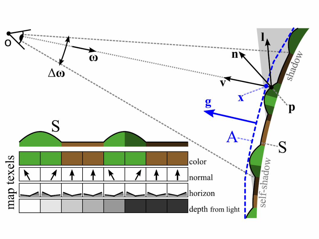
Introduction of aLocal Illumination Model
Change of variablesIntegral over surface maps
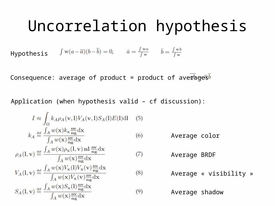
Uncorrelation hypothesisHypothesis
Consequence: average of product = product of averages
Application (when hypothesis valid – cf discussion):
Average color
Average BRDF
Average « visibility »
Average shadow

Parallax effects

Outline
● Using uncorrelation hypothesis & neglecting parallax:
– Color map filtering– Normal map filtering– Horizon map filtering– Shadow map filtering– Procedural map filtering– Summary
● Discussion of correlation & parallax effects● Conclusion

Color map filtering
● IF parallax effects neglected● THEN simple linear filtering of color map
→ Can use hardware anisotropic filtering
gives

Normal map filtering

Normal map filtering
● IF parallax effects neglected● THEN « simple » linear filtering of BRDF
● but BRDF = 4D function, not easy to store● Simplification hypothesis:
● BRDF represented with 2D distribution of normals
gives
normal map

Normal map filtering
● Direct methods● Represent fx with linear parameters, mipmap them
● Convolution methods● Further assume that● To use ergodicity relation● We get
● Represent px with linear parameters, mipmap them

Normal map filtering
● Representing 2D distributions:● Single Gaussian lobe represented with mean and
second moments (linear parameters)– 3D lobe, 2D lobe in tangent plane, isotropic or
anisotropic, etc– Second moments sometimes deduced from the mean
(Toksvig)● Multiple lobes● Spherical harmonics

Horizon map filtering

Horizon map filtering
● Fraction of S visible from viewer AND light
● Visibility represented with horizon map
● Reformulate with horizon distribution functions
● Or write V in a basis (e.g. Legendre Polynomials)
H = Heaviside function, non linear
V now linear in px!
Horizon map
(parallax effects neglected)

Horizon map filtering
● Representing horizon angle distributions:● Gaussian with mean and second moment
● Correlation between view and light directions: ● approximations
hotspot effect
[Ashikhmin et al.]
[Tan et al.]

Shadow map filtering

Shadow map filtering
● Average shadow (parallax neglected)
● Reformulate with depth distributions
● Or write S in a basis (e.g. use Fourier series)
H = Heaviside function, non linear
Shadow map (= depth map from light)
S now linear in ps!
gives
Other metod

Shadow map filtering
● Representing depth distributions● Gaussian with mean and second moment

Procedural map filtering

Procedural map filtering
● Global fading● Smooth transition from f(x) to its average● Drawback: attenuate ALL frequencies
● Analytic integration● Drawback: almost always impossible to compute
analytically● Workaround: apply on each term separately
● Frequency clamping● For methods using frequency synthesis (sum of
sinusoids, of trochoids, of noise functions, etc)

Summary
● To pre-filter a map M used in a non-linear function f(M,y)● Direct methods:
– use a « change of variable » to get f(M,y)=g(K,y) with g linear in the new variables K
– Pre-filter the new K variables● Convolution methods:
– Introduce the parameter distribution (= histogram) to get f(M,y)=∫f(m,y)px(m)dm, with px(m)=δ(m-Mx)
– Pre-filter linear parameters representing the px functions (e.g. mean and second moments, coefficients in a basis, etc). AND, at runtime, evaluate « convolution » f*pA

Summary
● Finding linear parameters characterizing a function:● Use moments● Use a basis of functions Bk
● Use a spanning set of functions
OR
→ spare representation
ki generally not linearly interpolable (counter-example: k = moments), requires alignment of « lobes »

Discussion
● Uncorrelation hypothesis● False for small footprints● Correlations between color and reflectance
– For each color channel, weight normals with reflectancel● Correlations between color and visibility● Correlations between reflectance and visibility● Correlations between view and light visibility
– Approximate solutions (cf above)

Discussion
● Parallax effects● Parallax offset
– Could be handled separately● Parallax Jacobian
– Not handled in existing works– Possible solution for normals

Discussion
● Silhouettes and curvature● Curvature and normal maps
– Curvature of base surface influences normals– Unless normals stored in global frame (instead of tangent
frame)● Curvature also influences horizon angles● Silhouettes
– Raw mesh resolution becomes visible● Silhouette clipping, shell mapping, relief mapping, etc
– Very anisotropic footprints

Discussion
● Mesh filtering and extreme filtering● At large distance, mesh itself must be pre-filtered● Removed mesh details must be incorporated in
surface maps (bump maps, normal maps, etc)● Topology changes can occur
– e.g. Tree foliage becomes a « volume » at large distance

Conclusion
● Many hard problems remain to be solved!


![· PK !^Æ2 '' mimetypeapplication/vnd.oasis.opendocument.textPK !öš ǃ ] META-INF/manifest.xml´—Ínà Çï“ö ÷@I·µEM« Vi‡íÔ=JœŒ *´jÞ~$R?vhµVñ- ëgcÿ10_î](https://static.fdocuments.in/doc/165x107/5b39307c7f8b9a4b0a8c849d/-pk-a2-mimetypeapplicationvndoasisopendocumenttextpk-oes-cf-meta-infmanifestxmlina.jpg)
![aravindavkgluster.readthedocs.ioaravindavkgluster.readthedocs.io/en/latest/presentations/... · Translate this pagePK ˆ‹]C3&¬¨// mimetypeapplication/vnd.oasis.opendocument.presentationPK](https://static.fdocuments.in/doc/165x107/5b360e237f8b9a3a6d8dd797/-translate-this-pagepk-c3-mimetypeapplicationvndoasisopendocumentpresentationpk.jpg)

