This page intentionally left blank - Politechnika Wrocł · PDF fileThis page intentionally...
162
Transcript of This page intentionally left blank - Politechnika Wrocł · PDF fileThis page intentionally...


This page intentionally left blank

A Student’s Guide to Fourier Transforms
Fourier transform theory is of central importance in a vast range of applications inphysical science, engineering and applied mathematics. Providing a conciseintroduction to the theory and practice of Fourier transforms, this book is invaluable tostudents of physics, electrical and electronic engineering and computer science.
After a brief description of the basic ideas and theorems, the power of the techniqueis illustrated through applications in optics, spectroscopy, electronics andtelecommunications. The rarely discussed but important field of multi-dimensionalFourier theory is covered, including a description of Computerized Axial Tomography(CAT) scanning. The book concludes by discussing digital methods, with particularattention to the Fast Fourier Transform and its implementation.
This new edition has been revised to include new and interesting material, such asconvolution with a sinusoid, coherence, the Michelson stellar interferometer and thevan Cittert–Zernike theorem, Babinet’s principle and dipole arrays.
j . f . james is a graduate of the University of Wales and the University of Reading.He has held teaching positions at the University of Minnesota, The Queen’s University,Belfast and the University of Manchester, retiring as Senior Lecturer in 1996. He is aFellow of the Royal Astronomical Society and a member of the Optical Society ofAmerica and the International Astronomical Union. His research interests include theinvention, design and construction of astronomical instruments and their use inastronomy, cosmology and upper-atmosphere physics. Dr James has led eclipseexpeditions to Central America, the central Sahara and the South Pacific Islands. He isthe author of about 40 academic papers, co-author with R. S. Sternberg of The Designof Optical Spectrometers (Chapman & Hall, 1969) and author of Spectrograph DesignFundamentals (Cambridge University Press, 2007).

A Student’s Guide to Fourier Transformswith Applications in Physics and Engineering
Third Edition
J. F. JAMES

cambridge university pressCambridge, New York, Melbourne, Madrid, Cape Town,
Singapore, Sao Paulo, Delhi, Tokyo, Mexico City
Cambridge University PressThe Edinburgh Building, Cambridge CB2 8RU, UK
Published in the United States of America by Cambridge University Press, New York
www.cambridge.orgInformation on this title: www.cambridge.org/9780521176835
C� J. F. James 2011
This publication is in copyright. Subject to statutory exceptionand to the provisions of relevant collective licensing agreements,no reproduction of any part may take place without the written
permission of Cambridge University Press.
First published 1995Second edition 2002Third edition 2011
Printed in the United Kingdom at the University Press, Cambridge
A catalogue record for this publication is available from the British Library
ISBN 978 0 521 17683 5 Paperback
Cambridge University Press has no responsibility for the persistence oraccuracy of URLs for external or third-party internet websites referred to
in this publication, and does not guarantee that any content on suchwebsites is, or will remain, accurate or appropriate.

Contents
Preface to the first edition page ixPreface to the second edition xiPreface to the third edition xiii
1 Physics and Fourier transforms 11.1 The qualitative approach 11.2 Fourier series 21.3 The amplitudes of the harmonics 41.4 Fourier transforms 81.5 Conjugate variables 101.6 Graphical representations 111.7 Useful functions 111.8 Worked examples 18
2 Useful properties and theorems 202.1 The Dirichlet conditions 202.2 Theorems 222.3 Convolutions and the convolution theorem 222.4 The algebra of convolutions 302.5 Other theorems 312.6 Aliasing 342.7 Worked examples 36
3 Applications 1: Fraunhofer diffraction 403.1 Fraunhofer diffraction 403.2 Examples 443.3 Babinet’s principle 543.4 Dipole arrays 55
v

vi Contents
3.5 Polar diagrams 583.6 Phase and coherence 583.7 Fringe visibility 603.8 The Michelson stellar interferometer 613.9 The van Cittert–Zernike theorem 64
4 Applications 2: signal analysis and communication theory 664.1 Communication channels 664.2 Noise 684.3 Filters 694.4 The matched filter theorem 704.5 Modulations 714.6 Multiplex transmission along a channel 774.7 The passage of some signals through simple filters 774.8 The Gibbs phenomenon 81
5 Applications 3: interference spectroscopy and spectral lineshapes 865.1 Interference spectrometry 865.2 The Michelson multiplex spectrometer 865.3 The shapes of spectrum lines 91
6 Two-dimensional Fourier transforms 976.1 Cartesian coordinates 976.2 Polar coordinates 986.3 Theorems 996.4 Examples of two-dimensional Fourier transforms with
circular symmetry 1006.5 Applications 1016.6 Solutions without circular symmetry 103
7 Multi-dimensional Fourier transforms 1057.1 The Dirac wall 1057.2 Computerized axial tomography 1087.3 A ‘spike’ or ‘nail’ 1127.4 The Dirac fence 1147.5 The ‘bed of nails’ 1157.6 Parallel-plane delta-functions 1167.7 Point arrays 1187.8 Lattices 119
8 The formal complex Fourier transform 120
Contents vii
9 Discrete and digital Fourier transforms 1279.1 History 1279.2 The discrete Fourier transform 1289.3 The matrix form of the DFT 1299.4 A BASIC FFT routine 133
Appendix 137Bibliography 141Index 143


Preface to the first edition
Showing a Fourier transform to a physics student generally produces the samereaction as showing a crucifix to Count Dracula. This may be because thesubject tends to be taught by theorists who themselves use Fourier methods tosolve otherwise intractable differential equations. The result is often a heavyload of mathematical analysis.
This need not be so. Engineers and practical physicists use Fourier theory inquite another way: to treat experimental data, to extract information from noisysignals, to design electrical filters, to ‘clean’ TV pictures and for many similarpractical tasks. The transforms are done digitally and there is a minimum ofmathematics involved.
The chief tools of the trade are the theorems in Chapter 2, and an easyfamiliarity with these is the way to mastery of the subject. In spite of the forestof integration signs throughout the book there is in fact very little integrationdone and most of that is at high-school level. There are one or two excursionsin places to show the breadth of power that the method can give. These are notpursued to any length but are intended to whet the appetite of those who wantto follow more theoretical paths.
The book is deliberately incomplete. Many topics are missing and there isno attempt to explain everything: but I have left, here and there, what I hopeare tempting clues to stimulate the reader into looking further; and of course,there is a bibliography at the end.
Practical scientists sometimes treat mathematics in general, and Fourier the-ory in particular, in ways quite different from those for which it was invented.1
The late E. T. Bell, mathematician and writer on mathematics, once describedmathematics in a famous book title as ‘The Queen and Servant of Science’.
1 It is a matter of philosophical disputation whether mathematics is invented or discovered. Letus compromise by saying that theorems are discovered; proofs are invented.
ix

x Preface to the first edition
The queen appears here in her role as servant and is sometimes treated quiteroughly in that role, and furthermore, without apology. We are fairly safe in theknowledge that mathematical functions which describe phenomena in the realworld are ‘well-behaved’ in the mathematical sense. Nature abhors singularitiesas much as she does a vacuum.
When an equation has several solutions, some are discarded in a mostcavalier fashion as ‘unphysical’. This is usually quite right.2 Mathematics isafter all only a concise shorthand description of the world and if a position-finding calculation based, say, on trigonometry and stellar observations, givestwo results, equally valid, that you are either in Greenland or Barbados, youare entitled to discard one of the solutions if it is snowing outside. So weuse Fourier transforms as a guide to what is happening or what to do next,but we remember that for solving practical problems the blackboard-and-chalkdiagram, the computer screen and the simple theorems described here are to bepreferred to the precise tedious calculations of integrals.
Manchester, January 1994 J. F. James
2 But Dirac’s equation, with its positive and negative roots, predicted the positron.

Preface to the second edition
This edition follows much advice and constructive criticism which the authorhas received from all quarters of the globe, in consequence of which vari-ous typos and misprints have been corrected and some ambiguous statementsand anfractuosities have been replaced by more clear and direct derivations.Chapter 7 has been largely rewritten to demonstrate the way in which Fouriertransforms are used in CAT scanning, an application of more than usual inge-nuity and importance: but overall this edition represents a renewed effort torescue Fourier transforms from the clutches of the pure mathematicians andpresent them as a working tool to the horny-handed toilers who strive in thefields of electronic engineering and experimental physics.
Glasgow, January 2001 J. F. James
xi


Preface to the third edition
Fourier transforms are eternal. They have not changed their nature since thelast edition ten years ago: but the intervening time has allowed the author tocorrect errors in the text and to expand it slightly to cover some other interestingapplications. The van Cittert–Zernike theorem makes a belated appearance, forexample, and there are hints of some aspects of radio aerial design as interestingapplications.
I also take the opportunity to thank many people who have offered criticism,often anonymously and therefore frankly, which has (usually) been acted uponand which, I hope, has improved the appeal both of the writing and of thecontents.
Kilcreggan, August 2010 J. F. James
xiii


1
1.1 The qualitative approach
Ninety percent of all physics is concerned with vibrations and waves of onesort or another. The same basic thread runs through most branches of physicalscience, from acoustics through engineering, fluid mechanics, optics, electro-magnetic theory and X-rays to quantum mechanics and information theory. Itis closely bound to the idea of a signal and its spectrum. To take a simpleexample: imagine an experiment in which a musician plays a steady note on atrumpet or a violin, and a microphone produces a voltage proportional to theinstantaneous air pressure. An oscilloscope will display a graph of pressureagainst time, F (t), which is periodic. The reciprocal of the period is the fre-quency of the note, 440 Hz, say, for a well-tempered middle A – the tuning-upfrequency for an orchestra.
The waveform is not a pure sinusoid, and it would be boring and colourlessif it were. It contains ‘harmonics’ or ‘overtones’: multiples of the fundamentalfrequency, with various amplitudes and in various phases,1 depending on thetimbre of the note, the type of instrument being played and on the player.The waveform can be analysed to find the amplitudes of the overtones, anda list can be made of the amplitudes and phases of the sinusoids which itcomprises. Alternatively a graph, A(ν), can be plotted (the sound-spectrum) ofthe amplitudes against frequency (Fig. 1.1).
A(ν) is the Fourier transform of F (t).
Actually it is the modular transform, but at this stage that is a detail.Suppose that the sound is not periodic – a squawk, a drumbeat or a crash
instead of a pure note. Then to describe it requires not just a set of overtones
1 ‘Phase’ here is an angle, used to define the ‘retardation’ of one wave or vibration with respectto another. One wavelength retardation, for example, is equivalent to a phase difference of 2π .Each harmonic will have its own phase, φm, indicating its position within the period.
1
Physics and Fourier transforms

2 Physics and Fourier transforms
Fig. 1.1. The spectrum of a steady note: fundamental and overtones.
with their amplitudes, but a continuous range of frequencies, each present inan infinitesimal amount. The two curves would then look like Fig. 1.2.
The uses of a Fourier transform can be imagined: the identification of avaluable violin; the analysis of the sound of an aero-engine to detect a faultygear-wheel; of an electrocardiogram to detect a heart defect; of the light curveof a periodic variable star to determine the underlying physical causes of thevariation: all these are current applications of Fourier transforms.
1.2 Fourier series
For a steady note the description requires only the fundamental frequency, itsamplitude and the amplitudes of its harmonics. A discrete sum is sufficient. Wecould write
F (t) D a0 C a1 cos(2πν0t)C b1 sin(2πν0t)C a2 cos(4πν0t)
C b2 sin(4πν0t)C a3 cos(6πν0t)C � � � ,
where ν0 is the fundamental frequency of the note. Sines as well as cosines arerequired because the harmonics are not necessarily ‘in step’ (i.e. ‘in phase’)with the fundamental or with each other.
More formally:
F (t) D1∑
nD�1
an cos(2πnν0t)C bn sin(2πnν0t) (1.1)
and the sum is taken from �1 to1 for the sake of mathematical symmetry.

1.2 Fourier series 3
Fig. 1.2. The spectrum of a crash: all frequencies are present.
This process of constructing a waveform by adding together a fundamentalfrequency and overtones or harmonics of various amplitudes is called Fouriersynthesis.
There are alternative ways of writing this expression: since cos x D cos(�x)and sin x D �sin(�x) we can write
F (t) D A0/2C1∑
nD1
An cos(2πnν0t)C Bn sin(2πnν0t) (1.2)
and the two expressions are identical, provided that we set An D a�n C an andBn D bn � b�n. A0 is divided by two to avoid counting it twice: as it is, A0 canbe found by the same formula that will be used to find all the An’s.

4 Physics and Fourier transforms
Mathematicians and some theoretical physicists write the expression as
F (t) D A0/2C1∑
nD1
An cos(nω0t)C Bn sin(nω0t)
and there are entirely practical reasons, which are discussed later, for not writingit this way.
1.3 The amplitudes of the harmonics
The alternative process – of extracting from the signal the various frequenciesand amplitudes that are present – is called Fourier analysis and is much moreimportant in its practical physical applications. In physics, we usually find thecurve F (t) experimentally and we want to know the values of the amplitudesAm and Bm for as many values of m as necessary. To find the values ofthese amplitudes, we use the orthogonality property of sines and cosines. Thisproperty is that, if you take a sine and a cosine, or two sines or two cosines,each a multiple of some fundamental frequency, multiply them together andintegrate the product over one period of that frequency, the result is always zeroexcept in special cases.
If P D 1/ν0 is one period, then∫ P
tD0cos(2πnν0t) � cos(2πmν0t)dt D 0
and ∫ P
tD0sin(2πnν0t) � sin(2πmν0t)dt D 0
unless m D ˙n, and∫ P
tD0sin(2πnν0t) � cos(2πmν0t)dt D 0
always.The first two integrals are both equal to 1/(2ν0) if m D n.We multiply the expression (1.2) for F (t) by sin(2πmν0t) and the product
is integrated over one period, P :∫ P
tD0F (t)sin(2πmν0t)dt D
A0
2
∫ P
tD0sin(2πmν0t)dt
C
∫ P
tD0
1∑nD1
fAn cos(2πnν0t)C Bn sin(2πnν0t)gsin(2πmν0t)dt (1.3)

1.3 The amplitudes of the harmonics 5
and all the terms of the sum vanish on integration except∫ P
0Bm sin2(2πmν0t)dt D Bm
∫ P
0sin2(2πmν0t)dt
D Bm/(2ν0) D BmP/2
so that
Bm D (2/P )∫ P
0F (t)sin(2πmν0t)dt (1.4)
and, provided that F (t) is known in the interval 0! P , the coefficient Bm canbe found. If an analytic expression for F (t) is known, the integral can often bedone. On the other hand, if F (t) has been found experimentally, a computer isneeded to do the integrations.
The corresponding formula for Am is
Am D (2/P )∫ P
0F (t)cos(2πmν0t)dt. (1.5)
The integral can start anywhere, not necessarily at t D 0, so long as it extendsover one period.
Example: Suppose that F (t) is a square-wave of period 1/ν0, so that F (t) Dh for t D �b/2! b/2 and 0 during the rest of the period, as in Fig. 1.3.Then
Am D 2ν0
∫ 1/(2ν0)
�1/(2ν0)F (t)cos(2πmν0t)dt
D 2hν0
∫ b/2
�b/2cos(2πmν0t)dt
and the new limits cover only that part of the cycle where F (t) is differentfrom zero.
Fig. 1.3. A rectangular wave of period 1/ν0 and pulse-width b.
6 Physics and Fourier transforms
If we integrate and put in the limits:
Am D2hν0
2πmν0fsin(πmν0b) � sin(�πmν0b)g
D2h
πmsin(πmν0b)
D 2hν0bfsin(πν0mb)/(πν0mb)g .
All the Bn’s are zero because of the symmetry of the function – wetook the origin to be at the centre of one of the pulses.
The original function of time can be written
F (t) D hν0bC 2hν0b
1∑mD1
fsin(πν0mb)/(πν0mb)gcos(2πmν0t) (1.6)
or, alternatively,
F (t) Dhb
PC
2hb
P
1∑mD1
fsin(πν0mb)/(πν0mb)gcos(2πmν0t). (1.7)
Notice that the first term, A0/2, is the average height of the function –the area under the top-hat divided by the period; and that the functionsin(x)/x, called ‘sinc(x)’, which will be described in detail later, has thevalue unity at x D 0, as can be shown using de l’Hopital’s rule.2
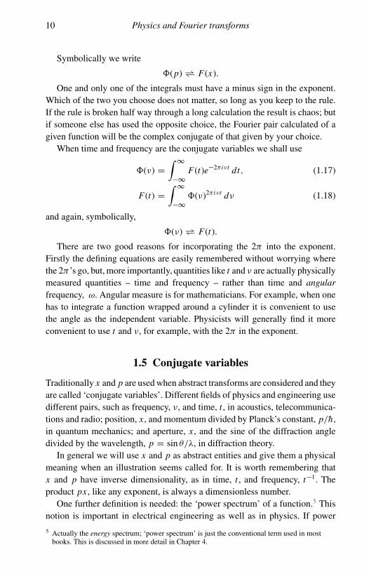
There are other ways of writing the Fourier series. It is convenient occasion-ally, though less often, to write Am D Rm cos φm and Bm D Rm sin φm, so thatequation (1.2) becomes
F (t) DA0
2C
1∑mD1
Rm cos(2πmν0t C φm) (1.8)
and Rm and φm are the amplitude and phase of the mth harmonic. A singlesinusoid then replaces each sine and cosine, and the two quantities needed todefine each harmonic are these amplitudes and phases in place of the previousAm and Bm coefficients. In practice it is usually the amplitude, Rm, which isimportant, since the energy in an oscillator is proportional to the square of theamplitude of oscillation, and jRmj
2 gives a measure of the power contained ineach harmonic of a wave. ‘Phase’ is a simple and important idea. Two wavetrains are ‘in phase’ if wave crests arrive at a certain point together. They are‘out of phase’ if a trough from one arrives at the same time as the crest of theother. (Alternatively, they have 180ı phase difference.) In Fig. 1.4 there are two
2 De l’Hopital’s rule is that, if f (x) ! 0 as x ! 0 and φ(x) ! 0 as x ! 0, the ratio f (x)/φ(x)is indeterminate, but is equal to the ratio (df/dx)/(dφ/dx) as x ! 0.

1.3 The amplitudes of the harmonics 7
Fig. 1.4. Two wave trains with the same period but different amplitudes andphases. The upper has 0.7 times the amplitude of the lower and there is a phase-difference of 70ı.
wave trains. The upper has 0.7 times the amplitude of the other and it lags (notleads, as it appears to do) the lower by 70ı. This is because the horizontal axisof the graph is time, and the vertical axis measures the amplitude at a fixedpoint as it varies with time. Wave crests from the lower wave train arrive earlierthan those from the upper. The important thing is that the ‘phase-difference’between the two is 70ı.
The most common way of writing the series expansion is with complexexponentials instead of trigonometrical functions. This is because the algebraof complex exponentials is easier to manipulate. The two ways are linked, ofcourse, by de Moivre’s theorem. We can write
F (t) D1∑
�1
Cme2πimν0t ,
where the coefficients Cm are now complex numbers in general and Cm D C��m.
(The exact relationship is given in detail in Appendix A.3.) The coefficientsAm, Bm and Cm are obtained from the inversion formulae:
Am D 2ν0
∫ 1/v0
0F (t)cos(2πmν0t)dt,
Bm D 2ν0
∫ 1/v0
0F (t)sin(2πmν0t)dt,
Cm D 2ν0
∫ 1/v0
0F (t)e�2πmν0t dt

8 Physics and Fourier transforms
(the minus sign in the exponent is important) or, if ω0 has been used instead ofν0 (ν0 D ω0/(2π )), then
Am D (ω0/π )∫ 2π/ω0
0F (t)cos(mω0t)dt,
Bm D (ω0/π )∫ 2π/ω0
0F (t)sin(mω0t)dt,
Cm D (2ω0/π )∫ 2π/ω0
0F (t)e�imω0t dt.
The useful mnemonic form to remember for finding the coefficients in a Fourierseries is
Am D2
period
∫one period
F (t)cos
{2πmt
period
}dt, (1.9)
Bm D2
period
∫one period
F (t)sin
{2πmt
period
}dt (1.10)
and remember that the integral can be taken from any starting point, a, providedthat it extends over one period to an upper limit a C P . The integral can besplit into as many subdivisions as needed if, for example, F (t) has differentanalytic forms in different parts of the period.
1.4 Fourier transforms
Whether F (t) is periodic or not, a complete description of F (t) can be givenusing sines and cosines. If F (t) is not periodic it requires all frequencies tobe present if it is to be synthesized. A non-periodic function may be thoughtof as a limiting case of a periodic one, where the period tends to infinity, andconsequently the fundamental frequency tends to zero. The harmonics are moreand more closely spaced and in the limit there is a continuum of harmonics,each one of infinitesimal amplitude, a(ν)dν, for example. The summation signis replaced by an integral sign and we find that
F (t) D∫ 1
�1
a(ν)dν cos(2πνt)C∫ 1
�1
b(ν)dν sin(2πνt) (1.11)
or, equivalently,
F (t) D∫ 1
�1
r(ν)cos(2πνt C φ(ν))dν (1.12)
or, again,
F (t) D∫ 1
�1
�(ν)e2πiνt dν. (1.13)

1.4 Fourier transforms 9
If F (t) is real, that is to say, if the insertion of any value of t into F (t) yieldsa real number, then a(ν) and b(ν) are real too. However, �(ν) may be complexand indeed will be if F (t) is asymmetrical so that F (t) 6D F (�t). This cansometimes cause complications, and these are dealt with in Chapter 8: but F (t)is often symmetrical and then �(ν) is real and F (t) comprises only cosines.We could then write
F (t) D∫ 1
�1
�(ν)cos(2πνt)dν
but, because complex exponentials are easier to manipulate, we take equation(1.13) above as the standard form. Nevertheless, for many practical purposesonly real and symmetrical functions F (t) and �(ν) need be considered.
Just as with Fourier series, the function �(ν) can be recovered from F (t) byinversion. This is the cornerstone of Fourier theory because, astonishingly, theinversion has exactly the same form as the synthesis, and we can write, if �(ν)is real and F (t) is symmetrical,
�(ν) D∫ 1
�1
F (t)cos(2πνt)dt, (1.14)
so that not only is �(ν) the Fourier transform of F (t), but also F (t) is theFourier transform of �(ν). The two together are called a ‘Fourier pair’.
The complete and rigorous proof of this is long and tedious3 and it is notnecessary here; but the formal definition can be given and this is a suitableplace to abandon, for the moment, the physical variables time and frequencyand to change to the pair of abstract variables, x and p, which are usually used.The formal statement of a Fourier transform is then
�(p) D∫ 1
�1
F (x)e2πipx dx, (1.15)
F (x) D∫ 1
�1
�(p)e�2πipx dp (1.16)
and this pair of formulae4 will be used from here on.
3 It is to be found, for example, in E. C. Titchmarsh, Introduction to the Theory of FourierIntegrals, Clarendon Press, Oxford, 1962 or in R. R. Goldberg, Fourier Transforms, CambridgeUniversity Press, Cambridge, 1965.
4 Sometimes one finds
�(p) D1
2π
∫ 1
�1F (x)eipx dx; F (x) D
∫ 1
�1�(p)e�ipx dp
as the defining equations, and again symmetry is preserved by some people by defining thetransform by
�(p) D
{1
2π
}1/2 ∫ 1
�1F (x)eipx dx; F (x) D
{1
2π
}1/2 ∫ 1
�1�(p)e�ipx dp.
10 Physics and Fourier transforms
Symbolically we write
�(p)• F (x).
One and only one of the integrals must have a minus sign in the exponent.Which of the two you choose does not matter, so long as you keep to the rule.If the rule is broken half way through a long calculation the result is chaos; butif someone else has used the opposite choice, the Fourier pair calculated of agiven function will be the complex conjugate of that given by your choice.
When time and frequency are the conjugate variables we shall use
�(ν) D∫ 1
�1
F (t)e�2πiνt dt, (1.17)
F (t) D∫ 1
�1
�(ν)2πiνt dν (1.18)
and again, symbolically,
�(ν)• F (t).
There are two good reasons for incorporating the 2π into the exponent.Firstly the defining equations are easily remembered without worrying wherethe 2π ’s go, but, more importantly, quantities like t and ν are actually physicallymeasured quantities – time and frequency – rather than time and angularfrequency, ω. Angular measure is for mathematicians. For example, when onehas to integrate a function wrapped around a cylinder it is convenient to usethe angle as the independent variable. Physicists will generally find it moreconvenient to use t and ν, for example, with the 2π in the exponent.
1.5 Conjugate variables
Traditionally x and p are used when abstract transforms are considered and theyare called ‘conjugate variables’. Different fields of physics and engineering usedifferent pairs, such as frequency, ν, and time, t , in acoustics, telecommunica-tions and radio; position, x, and momentum divided by Planck’s constant, p/h,in quantum mechanics; and aperture, x, and the sine of the diffraction angledivided by the wavelength, p D sin θ/λ, in diffraction theory.
In general we will use x and p as abstract entities and give them a physicalmeaning when an illustration seems called for. It is worth remembering thatx and p have inverse dimensionality, as in time, t , and frequency, t�1. Theproduct px, like any exponent, is always a dimensionless number.
One further definition is needed: the ‘power spectrum’ of a function.5 Thisnotion is important in electrical engineering as well as in physics. If power
5 Actually the energy spectrum; ‘power spectrum’ is just the conventional term used in mostbooks. This is discussed in more detail in Chapter 4.
1.7 Useful functions 11
is transmitted by electromagnetic radiation (radio waves or light) or by wiresor waveguides, the voltage at a point varies with time as V (t). �(ν), theFourier transform of V (t), may very well be – indeed usually is – complex.However, the power per unit frequency interval being transmitted is propor-tional to �(ν)��(ν), where the constant of proportionality depends on theload impedance. The function S(ν) = �(ν)��(ν) D j�(ν)j2 is called the powerspectrum or the spectral power density (SPD) of F (t). This is what an opticalspectrometer measures, for example.
1.6 Graphical representations
It frequently happens that greater insight into the physical processes which aredescribed by a Fourier transform can be achieved by use of a diagram ratherthan a formula. When a real function F (x) is transformed it generally producesa complex function �(p), which needs an Argand diagram to demonstrate it.Three dimensions are required: Re �(p), Im �(p) and p. A perspective drawingwill display the function, which appears as a more or less sinuous line. If F (x)is symmetrical, the line lies in the Re p-plane, whereas if it is antisymmetrical,the line lies in the Im p-plane. Figures 8.1 and 8.2 in Chapter 8 illustrate thispoint.
Electrical engineering students, in particular, will recognize the end-on viewalong the p-axis as the ‘Nyquist diagram’ of feedback theory. There will beexamples of this graphical representation in later chapters.
1.7 Useful functions
There are some functions which occur again and again in physics, and whoseproperties should be learned. They are extremely useful in the manipulation andgeneral taming of other functions which would otherwise be almost unman-ageable. Chief among these are the following.
1.7.1 The ‘top-hat’ function6
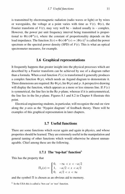
This has the property that
�a(x) D
0, �1 < x < �a/21, �a/2 < x < a/20, a/2 < x <1
and the symbol � is chosen as an obvious aid to memory.
6 In the USA this is called a ‘box-car’ or ‘rect’ function.

12 Physics and Fourier transforms
Fig. 1.5. The top-hat function and its transform, the sinc-function.
Its Fourier pair is obtained by integration:
�(p) D∫ 1
�1
�a(x)e2πipx dx
D
∫ a/2
�a/2e2πipx dx
D1
2πip[eπipa � e�πipa]
D a
{sin(πpa)
πpa
}D a sinc(πpa)
and the ‘sinc-function’, defined7 by sinc(x) = sin x/x, is one which recursthroughout physics (Fig. 1.5). As before, we write symbolically
�a(x)• a sinc(πpa).
1.7.2 The sinc-function
The sinc-function sinc(x) D sin x/x has the value unity at x D 0, and has zeroswhenever x D nπ . The function sinc(πpa) above, the most common form, haszeros when p D 1/a, 2/a, 3/a, . . .
7 Caution: some people define sinc(x) as sin(πx)/(πx), although without noticeable advantageand with occasional confusion when the argument is complicated.

1.7 Useful functions 13
1.665a
0.53/a
Fig. 1.6. The Gaussian function and its transform, another Gaussian with fullwidth at half maximum inversely proportional to that of its Fourier pair.
1.7.3 The Gaussian function
Suppose G(x) D e�x2/a2, where a is the ‘width parameter’ of the function. The
value of G(x) D 1/2 when (x/a)2 D loge2, or x D ˙0.8325a so that the fullwidth at half maximum (FWHM) is 1.665a and (which every scientist shouldknow!)
∫1
�1 e�x2/a2dx D a
pπ.
Its Fourier transform is g(p), given by
g(p) D∫ 1
�1
e�x2/a2e2πipx dx
(Fig. 1.6). The exponent can be rewritten (by ‘completing the square’) as
�(x/a � πipa)2 � π2p2a2

14 Physics and Fourier transforms
and then
g(p) D e�π2p2a2∫ 1
�1
e�(x/a�πipa)2dx.
Put x/a � πipa D z, so that dx D a dz. Then
g(p) D ae�π2p2a2∫ 1
�1
e�z2dz
D ap
πe�π2a2p2
so that g(p) is another Gaussian function, with width parameter 1/(πa).Notice that the wider the original Gaussian, the narrower will be its Fourier
pair.Notice, too, that the value at p D 0 of the Fourier pair is equal to the area
under the original Gaussian.
1.7.4 The exponential decay
This, in physics, is generally the positive part of the function e�x/a . It isasymmetrical, so its Fourier transform is complex:
�(p) D∫ 1
0e�x/ae2πipx dx
D
[e2πipx�x/a
2πip � 1/a
]1
0
D�1
2πip � 1/a.
Usually, with this function, the power spectrum is the most interesting:
j�(p)j2 Da2
4π2p2a2 C 1.
This is a bell-shaped curve, similar in appearance to a Gaussian curve, and isgenerally known as a Lorentz profile.8 Its FWHM is 1/(πa).
It is the shape found in spectrum lines when they are observed at very lowpressure, when collisions between emitting particles are infrequent comparedwith the transition probability. If the line profile is taken as a function offrequency, I (ν), the FWHM, ν, is related to the ‘lifetime of the excited state’,the reciprocal of the transition probability in the atom which undergoes thetransition. In this example, a and x obviously have dimensions of time. Looked
8 It is also known to mathematicians as the ‘Witch of Agnesi’ or more accurately as the ‘curve ofAgnesi’, having been studied by the eighteenth-century mathematician Maria Agnesi(1718–1799). The translator confused versiera – ‘curve’ – with avversiera – witch.
1.7 Useful functions 15
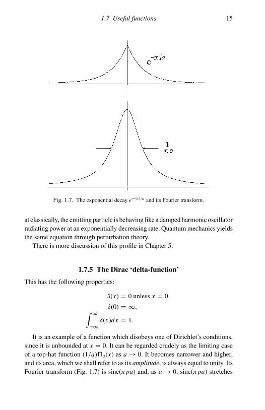
Fig. 1.7. The exponential decay e�jxj/a and its Fourier transform.
at classically, the emitting particle is behaving like a damped harmonic oscillatorradiating power at an exponentially decreasing rate. Quantum mechanics yieldsthe same equation through perturbation theory.
There is more discussion of this profile in Chapter 5.
1.7.5 The Dirac ‘delta-function’
This has the following properties:
δ(x) D 0 unless x D 0,
δ(0) D 1,∫ 1
�1
δ(x)dx D 1.
It is an example of a function which disobeys one of Dirichlet’s conditions,since it is unbounded at x D 0. It can be regarded crudely as the limiting caseof a top-hat function (1/a)�a(x) as a ! 0. It becomes narrower and higher,and its area, which we shall refer to as its amplitude, is always equal to unity. ItsFourier transform (Fig. 1.7) is sinc(πpa) and, as a ! 0, sinc(πpa) stretches

16 Physics and Fourier transforms
and in the limit is a straight line at unit height above the x-axis. In otherwords,
the Fourier transform of a delta-function is unity
and we write
δ(x)• 1.
Alternatively, and more accurately, it is the limiting case of a Gaussianfunction of unit area as it gets narrower and higher. Its Fourier transform thenis another Gaussian of unit height, getting broader and broader until in the limitit is a straight line at unit height above the axis.
Although the function has infinite height, we frequently encounter it multi-plied by a constant. In this case it is convenient, if not strictly accurate, to referto the function aδ(x) as having a ‘height’ a.
The following useful properties of the delta-function (or δ-function) shouldbe memorized. They are
δ(x � a) D 0 unless x D a
and the so-called ‘shift theorem’:∫ 1
�1
f (x)δ(x � a)dx D f (a),
where the product under the integral sign is zero except at x D a, where, onintegration, the δ-function has the amplitude f (a).
It is then easy to show, using this shift theorem, that for positive9 values ofa, b, c and d
δ(x/a � 1) D aδ(x � a).
To show this, put x D au; dx D a du. Then∫ 1
�1
δ(x/a � 1)f (x)dx D a
∫ 1
�1
δ(u � 1)f (au)du
and the integrand is zero except at the point u D 1, so that the result is af (a).Compare this with ∫ 1
�1
δ(x � a)f (x)dx D f (a)
and the substitution is obvious.
9 For negative values of these quantities a minus sign may be needed, bearing in mind that theintegral of a δ-function is always positive, even though a, for example, may be negative.Alternatively, we may write, for example, δ(x/a � 1) D jajδ(x � a).

1.7 Useful functions 17
Similarly, we find
δ(a/b � c/d) D acδ(ad � bc)
D bdδ(ad � bc)
δ(ax) D (1/a)δ(x).
Another important consequence of the shift theorem is that∫ 1
�1
e2πipxδ(x � a)dx D e2πipa
so that we can write
δ(x � a)• e2πipa,
δ(mx � a)• (1/m)e2πipa/m
and a formula which we shall need in Chapter 7:
1
nδ
(p
l�
r
n
)D δ
(pn
l� r
)• e�2πi( pn
l�r).
1.7.6 A pair of δ-functions
If two δ-functions are equally disposed on either side of the origin, the Fouriertransform is a cosine wave:
δ(x � a)C δ(x C a)• e2πipa C e�2πipa
D 2 cos(2πpa).
1.7.7 The Dirac comb
This is an infinite set of equally-spaced δ-functions, usually denoted by theCyrillic letter Ш (shah). Formally, we write
Шa(x) D1∑
nD�1
δ(x � na).
It is useful because it allows us to include Fourier series in the general theoryof Fourier transforms. For example, the convolution (to be described later) ofШa(x) and (1/b)�b(x) (where b < a) is a square wave similar to that in theearlier example, of period a and width b, and with unit area in each rectangle.The Fourier transform is then a Dirac comb, with ‘teeth’ of height am spacedat intervals 1/a. The am are, of course, the coefficients in the series.
If the square wave is allowed to become infinitesimally wide and infinitelyhigh so that the area under each rectangle remains unity, then the coefficients am

18 Physics and Fourier transforms
Fig. 1.8. A rectangular pulse-train with a 4 : 1 ‘mark–space’ ratio.
will all become of the same height, 1/a. In other words, the Fourier transformof a Dirac comb is another Dirac comb:
Шa(x)•1
aШ1/a(p)
and again notice that the period in p-space is the reciprocal of the period inx-space.
This is not a formal demonstration of the Fourier transform of a Dirac comb.A rigorous proof is much more elaborate, but is unnecessary here.
1.8 Worked examples
(1) A train of rectangular pulses, as in Fig. 1.8, has a pulse width equal to 1/4of the pulse period. Show that the 4th, 8th, 12th etc. harmonics are missing.
Taking zero at the centre of one pulse, the function is clearly symmetricalso that there are only cosine amplitudes:
An D2
P
∫ P/8
�P/8h cos
(2πnx
P
)dx
D
(h
πn
)2 sin
(2πn
P�P
8
)
D
(h
2
)sinc
(πn
4
)
so that An D 0 if n D 4, 8, 12, . . .
(2) Find the sine-amplitude of a sawtooth waveform as in Fig. 1.9.By choosing the origin half way up one of the teeth, the function is clearly
made antisymmetrical, so that there are no cosine amplitudes:
Bn D2
P
∫ P/2
�P/2
xh
Psin
(2πnx
P
)dx
D2h
P 2
[�x cos
(2πnx
P
)P
2πnC
P 2
4π2n2sin
(2πnx
P
)]P/2
�P/2
D [�2h/(πn)]cos(πn)

1.8 Worked examples 19
Fig. 1.9. A sawtooth waveform, antisymmetrical about the origin.
since sin(πn) D 0, so that
B0 D 0,
Bn D (�1)nC1[2h/(πn)], n 6D 0.
As a matter of interest, it is worthwhile calculating the sine-amplitudes whenthe origin is taken at the tip of a tooth, to see how changing the position of theorigin changes the amplitudes. It is also worthwhile doing the calculation for asimilar wave, with negative-going slopes instead of positive.

2
2.1 The Dirichlet conditions
Not all functions can be Fourier-transformed. They are transformable if theyfulfil certain conditions, known as the Dirichlet conditions.
The integrals which formally define the Fourier transform in Chapter 1 willexist if the integrands fulfil the following conditions:
� The functions F (x) and �(p) are square-integrable, i.e.∫1
�1 jF (x)j2 dx isfinite, which implies that F (x)! 0 as jxj ! 1.
� F (x) and �(p) are single-valued. For example, a curve such as that inFig. 2.1, despite having a respectable-looking Cartesian equation,1 is notFourier-transformable.
� F (x) and �(p) are ‘piece-wise continuous’. The function can be broken upinto separate pieces, so that there can be isolated discontinuities, as many asyou like, at the junctions, but the functions must be continuous, as definedfor instance by Weierstrass, between these discontinuities.2
� The functions F (x) and �(p) have upper and lower bounds. This is a con-dition which is sufficient but has not been proved necessary. In fact we shallassume that it is not. The Dirac δ-function, for instance, disobeys this con-dition. Figure 2.2 shows another example. No engineer or physicist has yetlost sleep over this one.
In Nature, all the phenomena that can be described mathematically seem torequire only well-behaved functions which obey the Dirichlet conditions. For
1 y D (x � 1)p
x.2 The classical nonconformist example is Dirichlet’s function, W (x), which has the property that
W (x) D 1 if x is rational and W (x) D 0 if x is irrational. It looks like a straight line but it is nottransformable, since it can be shown that between any two rational numbers, however close,there is at least one irrational number, and between any two irrational numbers there is at leastone rational number, so that the function is everywhere discontinuous.
20
Useful properties and theorems

2.1 The Dirichlet conditions 21
Fig. 2.1. A double-valued function like this is not Fourier-transformable.
Fig. 2.2. F (x) D 1/(x � a)2, an unbounded function of x which is not Fourier-transformable.

22 Useful properties and theorems
example, we can describe the electric field of a ‘wave-packet’ by a functionwhich is continuous, finite and single-valued everywhere, and, since the wave-packet contains only a finite amount of energy, the electric field is square-integrable.
2.2 Theorems
There are several theorems which are of great use in manipulating Fourier pairs,and they should be memorized. For the most part the proofs are elementary.The art of practical Fourier-transforming is in the manipulation of functionsusing these theorems, rather than in doing extensive and tiresome elementaryintegrations. It is this, as much as anything, which makes Fourier theory sucha powerful tool for the practical working scientist.
In what follows, we assume that
F1(x)• �1(p); F2(x)• �2(p),
where ‘•’ implies that F1 and �1 are a Fourier pair.The addition theorem states that
F1(x)C F2(x)• �1(p)C�2(p). (2.1)
The shift theorem already mentioned in Chapter 1 has the following lemmas:
F1(x C a)• �1(p)e2πipa,
F1(x � a)• �1(p)e�2πipa, (2.2)
F1(x � a)C F1(x C a)• 2�1(p)cos(2πpa).
In particular, notice that, if F1(x) is a δ-function, the lemmas are
δ(x C a)• e�2πipa,
δ(x � a)• e2πipa,
δ(x � a)C δ(x C a)• 2 cos(2πpa). (2.3)
The third of these is illustrated in Fig. 2.3.
2.3 Convolutions and the convolution theorem
Convolutions are an important concept, especially in practical physics, and theidea of a convolution can be illustrated simply by an example.
Imagine a ‘perfect’ spectrometer, plotting a graph of intensity against wave-length, of a monochromatic source of light of intensity S and wavelength λ0.

2.3 Convolutions and the convolution theorem 23
x = −a
1/a
p
0 x
x = a
Fig. 2.3. A pair of δ-functions and its transform.
Represent the spectral power density (‘the spectrum’, see Fig. 2.4) of the sourceby Sδ(λ � λ0). The spectrometer will plot the graph as kSδ(λ � λ0), where k
is a factor which depends on the throughput of the spectrometer, its geometryand its detector sensitivity.
No spectrometer is perfect in practice, and what a real instrument will plot inresponse to a monochromatic input is a continuous curve kSI (λ � λ0), whereI (λ) is called the ‘instrumental function’ and
∫1
�1 I (λ)dλ D 1.Now we inquire what the instrument will plot in response to a continuous
spectrum input. Suppose that the intensity of the source as a function of wave-length is S(λ). We assume that a monochromatic line at any wavelength λ1
will be plotted as a similarly shaped function kI (λ � λ1). Then an infinitesimalinterval of the spectrum can be considered as a monochromatic line, at λ1, say,and of intensity S(λ1)dλ1 and it is plotted by the spectrometer as a functionof λ:
dO(λ) D kS(λ1)dλ1I (λ � λ1)
and the intensity apparently at another wavelength λ2 is
dO(λ2) D kS(λ1)I (λ2 � λ1)dλ1.

24 Useful properties and theorems
Fig. 2.4. The spectrum of a monochromatic wave (a) entering and (b) leavinga spectrometer. The area under curve (b) must be unity – the same as the ‘area’under the δ-function – in order to preserve the idea of an ‘instrumental function’.
The total power apparently at λ2 is got by integrating this over all wave-lengths:
O(λ2) D k
∫ 1
�1
S(λ1)I (λ2 � λ1)dλ1
or, dropping unnecessary subscripts,
O(λ) D k
∫ 1
�1
S(λ1)I (λ � λ1)dλ1,
and the output curve, O(λ), is said to be the convolution of the spectrum S(λ)with the instrumental function I (λ).
It is the idea of an instrumental function, I (λ), which is important here. Weassume that the same shape I (λ) is given to any monochromatic line input.The idea extends to all sorts of measuring instruments and has various names,such as ‘impulse response’, ‘point-spread function’, ‘Green’s function’ and soon, depending on which branch of physics or electrical engineering is beingdiscussed. In an electronic circuit, for example, it answers the question ‘ifyou put in a sharp pulse, what comes out?’. Most instruments have no fixed

2.3 Convolutions and the convolution theorem 25
unique ‘instrumental function’, but the function often changes slowly enough(with wavelength, in the spectrometer example) that the idea can be used forpractical calculations.
The same idea can be envisaged in two dimensions: a point object – adistant star for instance – is imaged by a camera lens as a small smear of light,the ‘point-spread function’ of the lens. Even a ‘perfect’ lens has a diffractionpattern, so that the best that can be done is to convert a point object into an‘Airy-disc’ – a spot, 1.22f λ/d in diameter, where f is the focal length andd the diameter of the lens. The lens in general, when taking a photograph,gives an image which is the convolution, in two dimensions, of its point-spreadfunction with the object.
The formal definition of a convolution of two functions is then
C(x) D∫ 1
�1
F1(x0)F2(x � x0)dx0 (2.4)
and we write this symbolically as
C(x) D F1(x) � F2(x).
Convolutions obey various rules of arithmetic, and can be manipulated usingthem.
� The commutative rule:
C(x) D F1(x) � F2(x) D F2(x) � F1(x)
or
C(x) D∫ 1
�1
F2(x0)F1(x � x0)dx0
as can be shown by a simple substitution.� The distributive rule:
F1(x) � [F2(x)C F3(x)] D F1(x) � F2(x)C F1(x) � F3(x).
� The associative rule: the idea of a convolution can be extended to three ormore functions, and the order in which the convolutions are done does notmatter:
F1(x) � [F2(x) � F3(x)] D [F1(x) � F2(x)] � F3(x)
and usually the convolution of three functions is written without the squarebrackets:
C(x) D F1(x) � F2(x) � F3(x)
D
∫ 1
�1
∫ 1
�1
F1(x � x0)F2(x0 � x00)F3(x00)dx0 dx00.

26 Useful properties and theorems
In fact a whole algebra of convolutions exists and is very useful in tamingsome of the more fearsome-looking functions that are found in physics. Forexample,
[F1(x)C F2(x)] � [F3(x)C F4(x)] D F1(x) � F3(x)C F1(x) � F4(x)
C F2(x) � F3(x)C F2(x) � F4(x).
There is a way of visualizing a convolution. Draw the graph of F1(x). Draw,on a piece of transparent paper, the graph of F2(x). Turn the transparent graphover about a vertical axis and lay this mirror-image of F2 on top of the graph ofF1. When the two y-axes are displaced by a distance x0, integrate the productof the two functions. The result is one point on the graph of C(x0).
2.3.1 The convolution theorem
With the exception of Fourier’s inversion theorem, the convolution theorem isthe most astonishing result in Fourier theory. It is as follows.
If C(x) is the convolution of F1(x) with F2(x) then its Fourier pair, �(p),is the product of �1(p) and �2(p), the Fourier pairs of F1(x) and F2(x).Symbolically:
F1(x) � F2(x)• �1(p) ��2(p). (2.5)
The applications of this theorem are manifold and profound. Its proof iselementary:
C(x) D∫ 1
�1
F1(x0)F2(x � x0)dx0
by definition.Fourier transform both sides (and note that, because the limits are ˙1, x0
is a dummy variable and can be replaced by any other symbol not already inuse):
�(p) D∫ 1
�1
C(x)e2πipx dx D
∫ 1
�1
∫ 1
�1
F1(x0)F2(x � x0)e2πipx dx0 dx.
(2.6)
Introduce a new variable y D x � x0. Then, during the x-integration, x0 is heldconstant and dx D dy:
�(p) D∫ 1
�1
∫ 1
�1
F1(x0)F2(y)e2πip(x0Cy) dx0 dy,

2.3 Convolutions and the convolution theorem 27
which can be separated to give
�(p) D∫ 1
�1
F1(x0)e2πipx0
dx0 �
∫ 1
�1
F2(y)e2πipy dy
D �1(p) ��2(p).
2.3.2 Examples of convolutions
One of the chief uses of convolutions is to generate new functions which areeasy to transform using the convolution theorem.
Convolution of a function with a δ-function, δ(x � a), gives
C(x) D∫ 1
�1
F (x � x0)δ(x0 � a)dx0 D F (x � a)
by virtue of the properties of δ-functions. This can be written symbolicallyas
F (x) � δ(x � a) D F (x � a).
Applying the convolution theorem to this is instructive since it yields theshift theorem:
F (x)• �(p); δ(x � a)• e�2πipa
so that F (x � a) D F (x) � δ(x � a)• �(p)e�2πipa.
More interesting is the convolution of a pair of δ-functions with anotherfunction:
[δ(x � a)C δ(x C a)]• 2 cos(2πpa).
Hence
[δ(x � a)C δ(x C a)] � F (x)• 2 cos(2πpa) ��(p) (2.7)
and this is illustrated in Fig. 2.5.The Fourier transform of a Gaussian g(x) D e�x2/a2
is, from Chapter 1,ap
πe�π2p2a2. The convolution of two unequal Gaussian curves, e�x2/a2
�
e�x2/b2, can then be done, either as a tiresome exercise in elementary calculus,
or by application of the convolution theorem:
e�x2/a2� e�x2/b2
• abπe�π2p2(a2Cb2)

28 Useful properties and theorems
Fig. 2.5. Convolution of a pair of δ-functions with F (x), and its transform.
Fig. 2.6. The triangle function, �a(x), as the convolution of two top-hat functions.
and the Fourier transform of the right-hand side is
abp
πp
a2 C b2e�x2/(a2Cb2) (2.8)
so that we arrive at a useful practical result:
the convolution of two Gaussians of width parameters a and b
is another Gaussian of width parameterp
a2 C b2
or, to put it another way, the resulting half-width is the Pythagorean sum of thetwo component half-widths.
The convolution of two equal top-hat functions (Fig. 2.6) is a good exampleof the power of the convolution theorem. It can be seen by inspection that theconvolution of two top-hat functions, each of height h and width a, is going tobe a triangle, usually called the ‘triangle function’ and denoted by �a(x), withheight h2a and base length 2a.
The Fourier transform of this triangle function can be done by elementaryintegration, splitting the integral into two parts: x D �a ! 0 and x D 0! a.This, too, is tiresome. On the other hand, it is trivial to see that if h�a(x)•ah sinc(πpa) then h2a�a(x)• a2h2 sinc2(πpa) or, more usefully,
h�a(x)• ah sinc2(πpa)
since the height of the sinc2-function is the area under the triangle.

2.3 Convolutions and the convolution theorem 29
2.3.3 The autocorrelation theorem
This is superficially similar to the convolution theorem but it has a differentphysical interpretation. This will be mentioned later in connection with theWiener–Khinchine theorem. The autocorrelation function of a function F (x)is defined as
A(x) D∫ 1
�1
F (x0)F (x C x0)dx0.
The process of autocorrelation can be thought of as a multiplication of everypoint of a function by another point at distance x0 further on, and then summingall the products; or like a convolution as described earlier, but with identicalfunctions and without taking the mirror-image of one of the two.
There is a theorem similar to the convolution theorem. Beginning with thedefinition
A(x) D∫ 1
�1
F (x0)F (x C x0)dx0
Fourier transform both sides:
�(p) D∫ 1
�1
A(x)e2πipx dx D
∫ 1
�1
∫ 1
�1
F (x0)F (x C x0)e2πipx dx0 dx.
Let x C x0 D y. Then, if x0 is held constant, dx D dy:
�(p) D∫ 1
�1
∫ 1
�1
F (x0)F (y)e2πip(y�x0) dx0 dy,
which can be separated into
�(p) D∫ 1
�1
F (x)e�2πipx0
dx0 �
∫ 1
�1
F (y)e2πipy dy
D � (p) ��(p)
so that
A(x)• j�(p)j2.
It is worth noting that, since � (p) ��(p) is real, an autocorrelation isautomatically a symmetrical function of x. This is something which may beintuitively obvious anyway.
The Wiener–Khinchine theorem, to be described in Chapter 4, may bethought of as a physical version of this theorem. It says that, if F (t) representsa signal, then its autocorrelation is (apart from a constant of proportionality)the Fourier transform of its power spectrum, j�(ν)j2.

30 Useful properties and theorems
2.4 The algebra of convolutions
You can think of convolution as a mathematical operation analogous to addi-tion, subtraction, multiplication, division, integration and differentiation. Thereare rules for combining convolution with the other operations. It cannot be asso-ciated with multiplication for example, and in general
[A(x) � B(x)] � C(x) 6D A(x) � [B(x) � C(x)].
But convolution signs and multiplication signs can be exchanged acrossa Fourier transform symbol, and this is very useful in practice. Forexample,
[A(x) � B(x)] � [C(x) �D(x)]• [a(p) � b(p)] � [c(p) � d(p)].
(Obviously upper-case and lower-case letters have been used to associateFourier pairs.)
As further examples:
A(x) � [B(x) � C(x)]• a(p) � [b(p) � c(p)],
[A(x)C B(x)] � [C(x)CD(x)]• [a(p)C b(p)] � [c(p)C d(p)],
[A(x) � B(x)C C(x) �D(x)] � E(x)• [a(p) � b(p)C c(p) � d(p)] � e(p).
Insofar as we use Fourier transforms in physics and engineering, we are con-cerned mostly with functions and manipulations like this to solve problems, andfluency in this relatively easy algebra is the key to success. Computation, ratherthan calculation, is involved, and there is much software available to computeFourier transforms digitally. However, most computation is done using com-plex exponentials and these involve the full complex transform. A later chapterdeals with this subject.
2.4.1 Convolution of two δ-functions
The convolution of two δ-functions can be regarded as the limiting case of theconvolution of two Gaussians: in other words it is another δ-function,
Aδ(x) � Bδ(x) D ABδ(x),
and this follows, after a few lines of algebra, from the definition of the δ-functionas
lima!0
1
ap
π� e�x2/a2
.

2.5 Other theorems 31
2.5 Other theorems
2.5.1 The derivative theorem
If �(p) and F (x) are a Fourier pair F (x)• �(p), then
dF/dx • �2πip�(p).
Proofs are elementary. You can integrate dF/dx by parts or you can differen-tiate3 F (x):
F (x) D∫ 1
�1
�(p)e�2πipx dp.
Differentiate with respect to x:
dF/dx D
∫ 1
�1
�2πip�(p)e�2πipx dp
D �2πi
∫ 1
�1
p�(p)e�2πipx dp (2.9)
and the right-hand side is �2πi times the Fourier transform of p�(p).
Example 1: The top-hat function �a(x)• a sinc(πpa). If the top-hat func-tion is differentiated with respect to x, the result is a pair of δ-functionsat the points where the slope was infinite:
d�a(x)
dxD δ(x C a/2) � δ(x � a/2).
Transforming both sides gives
δ(x C a/2) � δ(x � a/2)• e�πipa � eπipa D �2i sin(πpa)
D �2πip[a sinc(πpa)].
The theorem extends to further derivatives:
dnF (x)/dxn • (�2πip)n�(p)
and much use is made of this in mathematics.
Example 2: If the moment of inertia about the y-axis of a symmetrical curveis infinite, its Fourier transform has a cusp at the origin. Because∫ 1
1
f (x)dx D φ(0),
3 A word of caution: this works only if F (x) is an analytic function obeying the Dirichletconditions. Do not try it with a δ-function or a Heaviside step-function, for instance.

32 Useful properties and theorems
if (∂2f
∂x2
)xD0
D �4π2∫ 1
�1
p2φ(p)dp D1
there is a discontinuity in (∂f/∂x) at the origin.
Example 3: The differential equation of simple harmonic motion is
md2F (t)/dt2 C kF (t) D 0,
where F (t) is the displacement of the oscillator from equilibrium at timet . If we Fourier-transform this equation, F (t) becomes �(ν) and d2F/dt2
becomes �4π2ν2�(ν). The equation then becomes
�(ν)(k/m � 4π2ν2) D 0,
which, apart from the trivial solution �(ν) D 0, requires
ν D ˙1
2π
√k
m
– and this is just a small taste of the power which is available for thesolution of differential equations using Fourier transforms.
2.5.2 The convolution derivative theorem
d
dx[F1(x) � F2(x)] D F1(x) �
dF2(x)
dxD
dF1(x)
dx� F2(x). (2.10)
The derivative of the convolution of two functions is the convolution ofeither of the two with the derivative of the other. The proof is simple and is leftas an exercise.
2.5.3 Parseval’s theorem
This is met under various guises. It is sometimes called ‘Rayleigh’s theorem’or simply the ‘power theorem’. In general it states that∫ 1
�1
F1(x)F �2 (x)dx D
∫ 1
�1
�1(p)��2 (p)dp, (2.11)
where the superscript � denotes a complex conjugate. The proof of the theoremis given in Appendix A.1.

2.5 Other theorems 33
Fig. 2.7. The sampling theorem.
Two special cases of particular interest are
1
P
∫ P
0jF (x)j2 dx D
1∑�1
(a2n C b2
n) DA2
0
4C
1
2
1∑1
[A2n C B2
n], (2.12)
which is used for finding the power in a periodic waveform, and∫ 1
�1
jF (x)j2 dx D
∫ 1
�1
j�(p)j2 dp (2.13)
for non-periodic Fourier pairs.
2.5.4 The sampling theorem
This is also known as the ‘cardinal theorem’ of interpolary function theory, andoriginated with Whittaker,4 who asked and answered the following question:how often must a signal be measured (sampled) in order that all the frequenciespresent should be detected? The answer is that the sampling interval must bethe reciprocal of twice the highest frequency present.
The theorem is best illustrated with a diagram (Fig. 2.7). The highestfrequency is sometimes called the ‘folding frequency’, or alternatively the‘Nyquist’ frequency, and is given the symbol νf .
Suppose that the frequency spectrum, �(ν), of the signal is symmetricalabout the origin and stretches from �νf to νf . The convolution of this with aDirac comb of period 2ν0 provides a periodic function and the Fourier transform
4 J. M. Whittaker, Interpolary Function Theory, Cambridge University Press, Cambridge, 1935.

34 Useful properties and theorems
of this periodic function is the product of a Dirac comb with the original signal(and, to be strict, its reflection in the origin): in other words it is the setof Fourier coefficients in the series representing the periodic function. Theperiodic function is known, provided that the coefficients are known, and thecoefficients are the values of the original signal F (t), at intervals 1/(2νf ),multiplied by a suitable constant. The more coefficients are known, the moreharmonics can be added to make the spectrum, and the more detail can beseen in the function when it is reconstructed. With the help of the interpolationtheorem (below) all the points between the sample points can be filled in.
Formally, the process can be written with F (t) and �(ν) a Fourier pair asusual. The Fourier transform of F (t)Шa(t) is∫ 1
�1
F (t)Шa(t)e�2πiνt dt D �(ν) �Ш1/a(ν).
Rewrite the left-hand side as∫ 1
�1
F (t)1∑
nD�1
δ(t � na)e�2πiνt dt D
1∑nD�1
∫ 1
�1
F (t)δ(t � na)e�2πiνt dt
D
1∑nD�1
F (na)e�2πiνna D �0(ν).
The left-hand side is now a Fourier series, so that �0(ν) is a periodic function,namely the convolution of �(ν) with a Dirac comb of period 1/a. The constraintis that �(ν) must occupy the interval �1/(2a) to 1/(2a) only; in other words,1/a is twice the highest frequency in the function F (t), in accordance with thesampling theorem.
2.6 Aliasing
In the sampling theorem it is strictly necessary that the signal should containno power at frequencies above the folding frequency. If it does, this power willbe ‘folded’ back into the spectrum and will appear to be at a lower frequency.If the frequency is νf C νa it will appear to be at νf � νa in the spectrum. Ifit is at twice the folding frequency, it will appear to be at zero frequency. Forexample, a sine-wave sampled at intervals a, 2π C a, 4π C a, . . . will give aset of samples which are identical. There are, in effect, ‘beats’ between thefrequency and the sampling rate. It is always necessary to take precautionswhen examining a signal in order to be sure that a given ‘spike’ correspondsto the apparent frequency. This can be done either by deliberate filtering ofthe incoming signal, or by making several measurements at different sampling

2.6 Aliasing 35
Fig. 2.8. A signal occupying a high alias of a fundamental in frequency space,and its recovery by deliberate undersampling or ‘demodulating’.
frequencies. The former is the obvious method but not necessarily the best: ifthe signal is in the form of a pulse and is in a noisy environment, a lot of thepower can be lost by filtering.
Aliasing can be put to good use. If the frequency band stretches from ν0 toν1, the empty frequency band between ν0 and 0 can be divided into a number ofequal frequency intervals each less than 2(ν1 � ν0). The sampling interval thenneed be only 1/[2(ν1 � ν0)] instead of 1/(2ν1). This is a way of demodulatingthe signal, and the spectrum that is recovered appears to occupy the first aliaseven though the original occupied a possibly much higher one. The process isillustrated in Fig. 2.8.
2.6.1 The interpolation theorem
This too comes from Whittaker’s interpolary function theory. If the signalsamples are recorded, the values of the signal in between the sample pointscan be calculated. The spectrum of the signal can be regarded as the productof the periodic function with a top-hat function of width 2νf . In the signal,each sample is replaced by the convolution of the sinc-function with the corre-sponding δ-function. Each sample, anδ(t � tn), is replaced by the sinc-function,an sinc(πνf ), and each sinc-function conveniently has zeros at the positions ofall the other samples (this is hardly a coincidence, of course) so that the signalcan be reconstructed from a knowledge of its samples, which are the coefficientsof the Fourier series which form its spectrum.
This is much used in practical physics, where digital recording of data iscommon, and generally the signal at a point can be well enough recovered by a
36 Useful properties and theorems
sum of sinc-functions over twenty or thirty samples on either side. The reasonfor this is that, unless there is a very large amplitude to a sample at some distantpoint, the sinc-function at a distance of 30π from the sample has fallen to sucha low value that it is lost in the noise. It depends obviously on practical detailssuch as the signal-to-noise ratio in the original data and, more importantly, onthe absence of any power at frequencies higher than the folding frequency.
Stated formally, the signal F (t) sampled at times 0, t0, 2t0, 3t0, 4t0, 5t0, . . .
can be computed at any intermediate point t as the sum
F (nt0 C t) DN∑
mD�N
F f(nCm)t0gsinc[π (m � t/t0)],
where N , infinite in theory, is about 20–30 in practice. The sum cannot becomputed accurately near the ends of the data stream and there is a loss of N
samples at each end unless fewer samples are taken there.
2.6.2 The similarity theorem
This is fairly obvious: if you stretch F (x) so that it is twice as wide, then �(p)will be only half as wide, but twice as high as it was. Formally,
if F (x)• �(p) then F (ax)• j(1/a)j�(p/a).
The proof is trivial, and it is done by substituting x D ay, dx D a dy; p Dz/a, dp D (1/a)dz. Because the integrals are between �1 and 1, the vari-ables for integration are ‘dummy’ variables and can be replaced by any othersymbol not already in use.
2.7 Worked examples
2.7.1 An arithmetical result using Parseval’s theorem
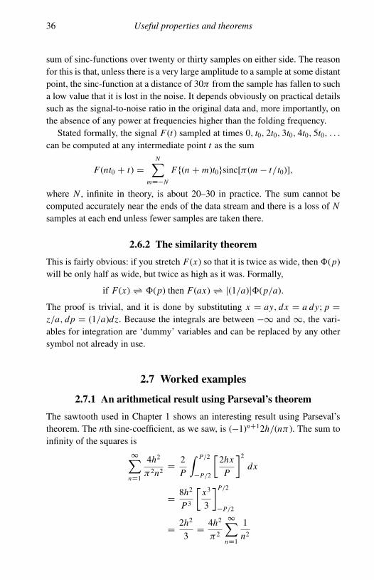
The sawtooth used in Chapter 1 shows an interesting result using Parseval’stheorem. The nth sine-coefficient, as we saw, is (�1)nC12h/(nπ ). The sum toinfinity of the squares is
1∑nD1
4h2
π2n2D
2
P
∫ P/2
�P/2
[2hx
P
]2
dx
D8h2
P 3
[x3
3
]P/2
�P/2
D2h2
3D
4h2
π2
1∑nD1
1
n2

2.7 Worked examples 37
so that finally
1∑nD1
1
n2D
π2
6.
This is an example of an arithmetical result coming from a purely analyticcalculation. As a way of computing π it is not very efficient: it is accurate toonly six significant figures (3.14159) after one million terms. Using the fact thatπ D 6 sin�1(1/2), with sin�1 obtained by integrating 1/
p1 � x2 term-by-term,
is much more efficient.
2.7.2 Alternating pulse-heights
In a rectangular waveform with pulses of length a/4 separated by spacesof length a/4 and with alternate rectangles twice the height of their neigh-bours, the amplitude of the second harmonic is greater than the fundamentalamplitude.
The waveform can be represented by
F (t) D h�a/4(t) � [Шa(t)CШa/2(t)].
The Fourier transform is
�(ν) D (ah/4)sinc(πνa/4) � [(1/a)Ш1/a(ν)C (2/a)Ш2/a(ν)]
and the teeth of this Dirac comb are at ν D 1/a, 2/a, . . . , with heights
(h/4)sinc(π/4), (3h/4)sinc(π/2), (h/4)sinc(3π/4) . . .
and the ratio of heights of the first and second harmonics isp
2 : 3.This effect can be seen in astronomy or radioastronomy when searching
for pulsars using a real-time Fourier transformer. The ‘interpulses’ betweenthe main pulses generate extra power in the second harmonic and can make itlarger than the fundamental (Fig. 2.9).
Fig. 2.9. A square-wave with alternating pulse heights. The Fourier transformwill show more power in the second harmonic than in the fundamental.

38 Useful properties and theorems
Fig. 2.10. The double-sawtooth waveform.
2.7.3 The double-sawtooth waveform
This cannot be regarded as the convolution of two rectangular waveforms ofequal mark–space5 ratio, since the effect of integration is to give an embarrass-ing infinity. Instead it is the convolution of a top-hat of width a with anotheridentical top-hat and with a Dirac comb of period 2a. Thus
�a(t) ��a(t) �Ш2a(t)• (a/2)sinc2(πνa) �Ш1/(2a)(ν).
So the amplitudes, which occur at ν D 1/(2a), 1/a, 3/(2a), . . . , are2a/π2, 0, 2a/(9π2), 0, 2a/(25π2), . . .
2.7.4 Convolution with a sinusoid
Consider an ordinary analytic function of x which obeys the Dirichlet conditionsand is neither symmetrical nor antisymmetrical. Its convolution with a cosineof unit amplitude and period 1/r is formally
C(x) D f (x) � cos(2πrx).
To calculate this convolution, first split the function f (x) into its symmetricaland antisymmetrical parts (see Fig. 8.1 for how to do this). Then
C(x) D [fs(x)C fa(x)] � cos(2πrx).
The Fourier transform of this is
�(p) D [φs(p)C iφa(p)] � [δ(p � r)C δ(p C r)]/2.
5 The term ‘equal mark–space ratio’ comes from radio jargon, and implies that the signal is zerofor the same interval as that during which it is not.

2.7 Worked examples 39
Γ(r ) d (p – r)
Γ(p)
Γ(r) d (p + r)
p
Fig. 2.11. Convolution of a function with a sinusoid. �(p) is the Fourier transformof f (x) and the two δ-functions are the Fourier transform of cos(2πrx), the otherpartner in the convolution. The product is the pair of δ-functions modified in heightby the appropriate Fourier component of �(p).
Notice that the product of a function with a δ-function is still a δ-function,i.e.
φ(p) � δ(p � r) D φ(r)δ(p � r).
Thus
�(p) D1
2[φs(r)δ(p � r)C φs(�r)δ(p C r)
C iφa(r)δ(p � r)C iφa(�r)δ(p C r)]
and, since φs(r) D φs(�r) and φa(r) D �φa(�r), we have
�(p) D1
2fφs(r)[δ(p � r)C δ(p C r)]C iφa(r)[δ(p � r) � δ(p C r)]g
and on transforming back we find
C(x) D φs(r)cos(2πrx)C φa(r)sin(2πrx)
so that C(x) is a sinusoid of amplitude√
φs(r)2 C φa(r)2 and phase-shifted bycomparison with the original sinusoid by an angle α, given by
α D tan�1[φa(r)/φs(r)].
This result (see Fig. 2.11) is important in the next chapter when we considerthe Michelson stellar interferometer and the van Cittert–Zernike theorem.

3
3.1 Fraunhofer diffraction
The application of Fourier theory to Fraunhofer diffraction problems, andto interference phenomena generally, was hardly recognized before the late1950s. Consequently, only textbooks written since then mention the tech-nique. Diffraction theory, of which interference is only a special case, derivesfrom Huygens’ principle: that every point on a wavefront which has comefrom a source can be regarded as a secondary source; and that all the wave-fronts from all these secondary sources combine and interfere to form a newwavefront.
Some precision can be added by using calculus. In Fig. 3.1, suppose that atO there is a source of ‘strength’ q, defined by the fact that at A, a distance r
from O, there is a ‘field’, E, of strength E D q/r . Huygens’ principle is nowas follows:
If we consider an area dS on the surface S we can regard it as a source of strengthE dS giving at B, a distance r 0 from A, a field E0 D q dS/(rr 0). All theseelementary fields at B, summed over the transparent part of the surface S, eachwith its proper phase,1 give the resultant field at B. This is quite general – andvague.
In elementary Fraunhofer diffraction theory we simplify. We assume thefollowing.
� That only two dimensions need be considered. All apertures bounding thetransparent part of the surface S are rectangular and of length unity perpen-dicular to the plane of the diagram.
1 Remember: phase change D (2π/λ) � path change and the paths from different points on thesurface S (which, being a wavefront, is a surface of constant phase) to B are all different.
40
Applications 1: Fraunhofer diffraction

3.1 Fraunhofer diffraction 41
Fig. 3.1. Secondary sources in Fraunhofer diffraction.
Fig. 3.2. Fraunhofer diffraction by a plane aperture.
� That the dimensions of the aperture are small compared with r 0.� That r is very large so that the field E has the same magnitude at all points on
the transparent part of S, and a slowly varying or constant phase. (Anotherway of putting it is to say that plane wavefronts arrive at the surface S froma source at �1.)
� That the aperture S lies in a plane.
To begin, suppose that the source, O, lies on a line perpendicular to thesurface S, the diffracting aperture. Use Cartesian coordinates, x in the plane ofS, and z perpendicular to this (x and z are traditional here; see Fig. 3.2). Thenthe magnitude of the field E at P can be calculated.

42 Applications 1
Consider an infinitesimal strip at Q, of unit length perpendicular to the x, z-plane, of width dx and distance x above the z-axis. Let the field strength2 therebe E D E0e
2πiνt . Then the field strength at P from this source will be
dE(P ) D E0e2πiνt e�2πir 0/λ dx,
where r 0 is the distance QP . The exponent in this last factor is the phasedifference between Q and P .
For convenience, choose a time t so that the phase of the wavefront is zeroat the plane S, i.e. t D 0. Then at P
E(P ) D∫
aperture,SE0e
�2πir 0/λ dx
and the aperture S may have opaque spots or partially transmitting spots, sothat E0 is generally a function of x.
This is not yet a useable expression.Now, because r 0 � x (the condition for Fraunhofer diffraction), we can
write
r 0 � r0 � x sin θ
and then the field E at P is obtained by summing all the infinitesimal contri-butions from the secondary sources like that at Q, and remembering to includethe phase-factor for each. The result is
E D E0e�2πir0/λ
∫aperture
e2πix sin θ/λ dx
and if we write sin θ/λ D p we have, finally,
E D E0e�2πir0/λ
∫ 1
�1
A(x)e2πipx dx,
where A(x) is the ‘aperture function’ which describes the transparent andopaque parts of the screen S. The result of the Fourier transform is to give theamplitude diffracted through an angle θ . Where it appears on a screen dependson the distance to the screen, and on whether the screen is perpendicular to thez-direction and other geometrical factors.3
The important thing to remember is this: that diffraction of a certain wave-length at a certain aperture is always through an angle: the variable p conjugate
2 As usual, we use complex variables to represent real quantities – in this case the electric fieldstrength. This complex variable is called the ‘analytic’ signal and the real part of it representsthe actual physical quantity at any time at any place.
3 This is all an approximation: in fact the field outside the diffracting aperture is not exactly zeroand depends in practice on whether the opaque part of the screen is conducting or insulatingand on the direction of polarization of the passing light. These are subtleties which can safelybe left to post-graduate students.

3.1 Fraunhofer diffraction 43
Fig. 3.3. Oblique incidence from a source not on the z-axis.
to x is sin θ/λ and it is θ which matters. Diffraction theory alone says nothingabout the size of the pattern: that depends on geometry.
Very often, in practice, the diffracting aperture is followed by a lens, andthe pattern is observed at the focal plane of this lens. The approximation thatr 0 D r0 � x sin θ is now exact, since the image of the focal plane, seen fromthe diffracting aperture, is at infinity.
Problems in Fraunhofer diffraction can thus be reduced to writing downthe aperture function, A(x), and taking its Fourier transform. The result givesthe amplitude in the diffraction pattern on a screen at a large distance from theaperture. For example, for a simple parallel-sided slit of width a, the aperturefunction, A(x), is �a(x). For two parallel-sided slits of width a separated by adistance b between their centres, A(x) D �a(x) � [δ(x � b/2)C δ(x C b/2)],and so on. Apertures of various sizes are now encompassed by the same formulaand the amplitude of the light (or sound, or radio waves or water waves)diffracted by the aperture through an angle θ can be calculated. The intensity ofthe wave is given by the r.m.s. value of the amplitude multiplied by its complexconjugate and the factor e2πir0/λ disappears when this is done.
If the original source is not on the z-axis, then the amplitude of E at z D 0contains a phase factor, as in Fig. 3.3.

44 Applications 1
Fig. 3.4. The intensity pattern, sinc2(πa sin θ/λ), from diffraction at a single slit.
W �W 0 is a wavefront (a surface of constant phase) and, if we choose amoment when the phase is zero at the origin, the phase at x at that momentis given by (2π/λ)x � sin φ, and the phase factor that must multiply E0 ise(�2π/λ)x sin φ .
The magnitude at P is then
E D E0e2πir0/λ
∫ 1
�1
A(x)e(�2πi/λ)x(sin θCsin φ) dx
and when the Fourier transform is done, the oblique incidence is accounted forby remembering that p D (sin θ C sin φ)/λ.
3.2 Examples
3.2.1 Single-slit diffraction, normal incidence
For a single slit with parallel sides, of width a, the aperture function is A(x) D�a(x). Then
E D k � sinc(πap) D k � sinc(πa sin θ/λ)
(where k is the constant4 E0ae�2πir0/λ), and the intensity is this multiplied byits complex conjugate:
EE� D I (θ ) D jkj2 � sinc2(πa sin θ/λ). (3.1)
See Fig. 3.4.
4 For most practical purposes, the unimportant constant.

3.2 Examples 45
Fig. 3.5. The intensity pattern from interference between two point sources.
3.2.2 Two point sources at˙b/2 (for example, two antennae,transmitting in phase from the same oscillator)
We have
A(x) D δ(x � b/2)C δ(x C b/2)
and the Fourier transform of this is (Chapter 1, equation (1.19))
E D 2k � cos(πb sin θ/λ)
and the intensity is this amplitude multiplied by its complex conjugate:
I (θ ) D 4jkj2 � cos2(πb sin θ/λ)
D 2jkj2[1C cos(2πb sin θ/λ)].
See Fig. 3.5.
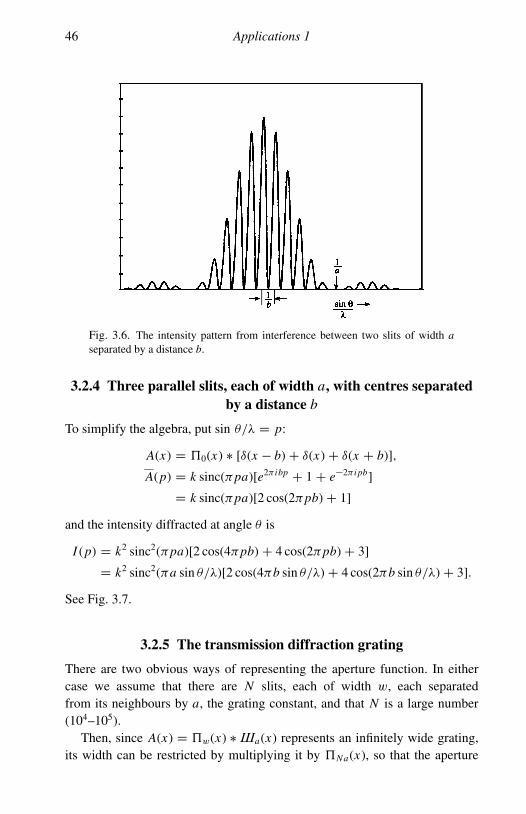
3.2.3 Two slits, each of width a, with centres separated by adistance b (Young’s slits, Fresnel’s biprism, Lloyd’s mirror,
Rayleigh’s refractometer, Billet’s split-lens)
We have
A(x) D �a(x) � [δ(x � b/2)C δ(x C b/2)].
Then, applying the convolution theorem,
I (θ ) D 4k2 sinc2(πa sin θ/λ)cos2(πb sin θ/λ).
See Fig. 3.6.
46 Applications 1
Fig. 3.6. The intensity pattern from interference between two slits of width a
separated by a distance b.
3.2.4 Three parallel slits, each of width a, with centres separatedby a distance b
To simplify the algebra, put sin θ/λ D p:
A(x) D �0(x) � [δ(x � b)C δ(x)C δ(x C b)],
A(p) D k sinc(πpa)[e2πibp C 1C e�2πipb]
D k sinc(πpa)[2 cos(2πpb)C 1]
and the intensity diffracted at angle θ is
I (p) D k2 sinc2(πpa)[2 cos(4πpb)C 4 cos(2πpb)C 3]
D k2 sinc2(πa sin θ/λ)[2 cos(4πb sin θ/λ)C 4 cos(2πb sin θ/λ)C 3].
See Fig. 3.7.
3.2.5 The transmission diffraction grating
There are two obvious ways of representing the aperture function. In eithercase we assume that there are N slits, each of width w, each separatedfrom its neighbours by a, the grating constant, and that N is a large number(104–105).
Then, since A(x) D �w(x) �Шa(x) represents an infinitely wide grating,its width can be restricted by multiplying it by �Na(x), so that the aperture

3.2 Examples 47
Fig. 3.7. The intensity pattern from interference between three slits of width a,separated by b.
function is
A(x) D �Na(x) � [�w(x) �Шa(x)].
Then the diffraction amplitude is
E(θ ) D Na � sinc(πNa sin θ/λ) � [w � sinc(πw sin θ/λ) � (1/a)Ш1/a(sin θ/λ)]
D Nw � sinc(πNa sin θ/λ) � [sinc(πw sin θ/λ) �Ш1/a(sin θ/λ)].
(N.B. The convolution is with respect to sin θ/λ.)A diagram here is helpful, see Fig. 3.8: the second factor (in the square
brackets) is the product of a Dirac comb and a very broad (because w is verysmall) sinc-function; and the convolution of this with the first factor, a verynarrow sinc-function, represents the diffraction produced by the whole apertureof the grating. Since the narrow sinc-function is reduced to insignificance bythe time it has reached as far as the next tooth in the Dirac comb, the intensitydistribution is this very narrow line profile sinc2(πNa sin θ/λ), reproduced ateach tooth position with its intensity reduced by the factor sinc2(πwa sin θ/λ).
This is not precise, but is close enough for all practical purposes. To beprecise, fastidious and pedantic, the aperture function, as described in the olderoptics textbooks, is
A(x) DN�1∑nD0
δ(x � na) ��w(x)

48 Applications 1
Fig. 3.8. The amplitude transmitted by a diffraction grating.
and since δ(x � na)• e2πinpa the diffracted amplitude is
E(θ ) D k � sinc(πwp)N�1∑nD0
e2πinpa,
where k D w � E0e�2πir0/λ. The third factor in the equation is the sum of a
geometrical progression of common ratio e2πipa and, after a few lines of algebra,the equation becomes
E(θ ) D k � sinc(πwp)eπi(N�1)pa sin(πNpa)/sin(πpa)
with p D sin θ/λ as usual.The intensity is given by E(θ )E(θ )�. The exponential factor disappears
together with its own complex conjugate and if we write I0 for E20 the intensity
distribution is
I (θ ) D I0 �
(sin(πNpa)
sin(πpa)
)2
sinc2(πwp). (3.2)
If N is large, the first factor is very similar to a sinc2-function, especially nearthe origin, where sin(πpa) ' πpa, and although it is exact it yields no moreinformation about the diffraction pattern details than the previous approximatederivation. Either way, the factor in the first bracket gives details about theline shape and the resolution to be obtained, and the third factor, the broadsinc2-function, gives information about the intensities of the various diffractionmaxima in the pattern.
In particular, if a maximum for one wavelength λ falls at the same diffrac-tion angle θ as the first zero of an adjacent wavelength λC δλ (the usual

3.2 Examples 49
Fig. 3.9. The shape of a spectrum line from a grating. The profile has the formsinc2(πNap).
criterion for resolution in a grating spectrometer), the two values of p can becompared:
for λ at maximum, sin θ � θ D mλ/a;
for λ at first zero, θ D mλ/a C λ/(Na),
which is the same angle as for λC δλ at maximum, i.e. m(λC δλ)/a,whence
δλ D λ/(mN ),
which gives the theoretical resolution of the grating.Two points are worth noting.
(1) No one expects to get the full theoretical resolution from a grating. Manu-facturing imperfections may reduce it in practice to�70% of the theoreticalvalue.
(2) Although this is the closest spacing for which two wavelengths can stillproduce separate images, more closely spaced wavelengths can be disen-tangled if the combined shape is known. The process of deconvolution canbe used to enhance resolution if need be, although the improvement can bedisappointing.
The sinc2-function in Fig. 3.9 represents the radiation intensity near thediffraction image of a monochromatic spectrum line. Although the diffractionintensity corresponds to a direction, θ , in practice a lens or a mirror will focus

50 Applications 1
Fig. 3.10. A diffraction grating with a diamond-shaped apodizing mask.
all the radiation that comes from the grating at that angle θ to a place on itsfocal surface where the CCD or other photo-sensitive detector is located.
The intensity distribution in the image will be the square modulus of theamplitude distribution, in this case a sinc2-function, which has its width5 deter-mined by the width Na of the grating.
The minima at λ0 and λ00 are at a wavelength difference˙1/(Na), from theproperties of the sinc2-function.
Interesting things can be done to the amplitude of the radiation transmitted(or reflected) by the grating by covering the grating with a mask. A diamond-shaped mask, for example (Fig. 3.10), will change the aperture function from�a(x) to �a(x) and the Fourier transform of the aperture function is then
E(θ ) D k � sinc2(π (aN/2)sin θ/λ) � [sinc(πw sin θ/λ) � (1/a)Ш1/a(sin θ/λ)].
The shape of the image of a monochromatic line is changed. Instead ofsinc2[πNa(sin θ/λ)], it becomes sinc4[(πNa/2)(sin θ/λ)]. The sinc4-functionis nearly twice as wide as the sinc2-function and the peak intensity of the lightis reduced by a factor of 4, but the intensities of the ‘side-lobes’ are reducedfrom 1.6 � 10�3 to 2.56 � 10�6 of the main peak intensity. This reduction isimportant if faint satellite lines are to be identified – for example in studiesof fine structure or Raman-scattered lines, where the satellite intensities are10�6 of the parent or less. The process, which is widely used in optics andradioastronomy, is called apodizing.6
5 By ‘width’ we mean here the full width at half maximum intensity of the spectrum line, usuallydenoted by ‘FWHM’.
6 From the Greek ‘without feet’, implying that the side-lobes are reduced or removed.
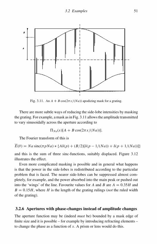
3.2 Examples 51
Fig. 3.11. An A C B cos(2πx/(Na)) apodizing mask for a grating.
There are more subtle ways of reducing the side-lobe intensities by maskingthe grating. For example, a mask as in Fig. 3.11 allows the amplitude transmittedto vary sinusoidally across the aperture according to
�Na(x)[AC B cos(2πx/(Na))].
The Fourier transform of this is
E(θ ) D Na sinc(πpNa) � fAδ(p)C (B/2)[δ(p � 1/(Na))C δ(p C 1/(Na))]g
and this is the sum of three sinc-functions, suitably displaced. Figure 3.12illustrates the effect.
Even more complicated masking is possible and in general what happensis that the power in the side-lobes is redistributed according to the particularproblem that is faced. The nearer side-lobes can be suppressed almost com-pletely, for example, and the power absorbed into the main peak or pushed outinto the ‘wings’ of the line. Favourite values for A and B are A D 0.35H andB D 0.15H , where H is the length of the grating rulings (not the ruled widthof the grating).
3.2.6 Apertures with phase-changes instead of amplitude changes
The aperture function may be (indeed must be) bounded by a mask edge offinite size and it is possible – for example by introducing refracting elements –to change the phase as a function of x. A prism or lens would do this.

52 Applications 1
Fig. 3.12. The intensity-profile of a spectrum line from a grating with a sinusoidalapodizing mask. The upper curve is the lower curve multiplied by 1000 to showthe low level of the secondary maxima.
3.2.7 Diffraction at an aperture with a prism
Because the ‘optical’ path is n times the geometrical path, the passage of lightthrough a distance x in a medium of refractive index n introduces an extra ‘path’(n � 1)x compared with the same length of path in air or vacuum. Consequentlythere is a phase change (2π/λ)(n � 1)x.
There is thus (Fig. 3.13) a variation of phase instead of transmission acrossthe aperture, so that the aperture function is complex. If the prism angle is φ
and the aperture width is a, the thickness of the prism at its base is a tan φ and,when parallel wavefronts coming from�1 have passed through the prism, thephases at the apex and the base of the prism are 0 and (2π/λ)(n � 1)a tan φ.
However, we can choose the phase to be zero at the centre of the aperture,and this is usually a good idea because it saves unnecessary algebra later on.
Then the phase at any point x in the aperture is ζ (x) = (2π/λ)x(n � 1)tan φ
and the aperture function describing the Huygens wavelets is
A(x) D �a(x)e(2πi/λ)x(n�1) tan φ.
The Fourier transform of this, with p D sin θ/λ as usual, is
E(θ ) D A
∫ a/2
�a/2e(2πi/λ)x(n�1)tan φe2πipx dx
so that, after integrating and multiplying the amplitude distribution by its com-plex conjugate, we get
I (θ ) D A2a2 sinc2faπ [p C (n � 1)tan φ/λ]g .

3.2 Examples 53
P
oz
x
Fig. 3.13. A single-slit aperture with a prism and its displaced diffractionpattern.
Notice that if n D 1 we have the same expression as in equation (3.1). Herewe see that the shape of the diffraction function is identical, but that the principalmaximum is shifted to the direction p D sin θ/λ D �(n � 1)tan φ/λ or to thediffraction angle θ D sin�1[(n � 1)tan φ]. This is what would be expected fromelementary geometrical optics when θ and φ are small.
3.2.8 The blazed diffraction grating
It is only a small step to the description of the diffraction produced by a gratingwhich comprises, instead of alternating opaque and transparent strips, a gridof parallel prisms. There are two advantages in such a construction. Firstly theaperture is completely transparent and no light is lost; and secondly the prismarrangement means that, for one wavelength at least, all the incident light isdiffracted into one order of the spectrum.
The aperture function is, as before, the convolution of the function for asingle slit with a Dirac comb, the whole being multiplied by a broad �Na(x)representing the whole width of the grating.
The diffracted intensity is then the same shifted sinc2-function as above, butmultiplied by the convolution of a Dirac comb with a narrow sinc-function, theFourier pair of �Na(x), which represents the shape of a single spectrum line.Now, there is a difference, because the broad sinc-function produced by a singleslit has the same width as the spacing of the teeth in the Dirac comb. The zeros

54 Applications 1
of this broad sinc-function are adjusted accordingly, and for one wavelengththe first order of diffraction falls on its maximum, while all the other ordersfall on its zeros. For this wavelength, all the transmitted light is diffracted intothe first order. For adjacent wavelengths the efficiency is similarly high, and ingeneral the efficiency remains usefully high for wavelengths between 2/3 and3/2 of this wavelength.
This is the ‘blaze wavelength’ of the grating and the corresponding angle θ
is the ‘blaze-angle’.Reflection gratings are made by ruling lines on an aluminium surface with
a diamond scribing tip, held at an angle to the surface so as to produce a seriesof long thin mirrors, one for each ruling. The angle is the ‘blaze-angle’ that thegrating will have, and a similar analysis will show easily that the phase-changeacross one slit is (2π/λ)2a tan β, where β is the ‘blaze-angle’ and a the widthof one ruling (and the separation of adjacent rulings). In practice, gratings areusually used with light incident normally or near-normally on the ruling facets,that is at an incidence angle β to the surface of the grating. There is then aphase-change of zero across one ruling, but a delay (2π/λ)2a sin θ betweenreflections from adjacent rulings. If this phase-change equals 2π then there isa principal maximum in the diffraction pattern.
Transmission gratings, generally found in undergraduate teaching laborato-ries, are usually blazed, and the effect can easily be seen by holding one up tothe eye and looking at a fluorescent lamp through it. The diffracted images invarious colours are much brighter on one side than on the other.
3.3 Babinet’s principle
This is a neglected but useful corollary of Fraunhofer diffraction theory. It says,in effect, that the Fraunhofer diffraction pattern from any aperture is the sameas that from the complementary obstruction. In other words, if the screen isremoved and an opaque object of the same shape as the screen aperture is putin the same place, the same diffraction pattern will be seen. The reasoning issimple: if there were no screen, the amplitude scattered at an angle θ wouldbe zero. If there is a screen with an aperture, there is a (complex) scatteringamplitude A(θ ). It follows then that if the screen is removed an amplitude�A(θ ) has been added to cancel out the first. That amplitude must have comefrom the obstructing part of the screen, and if that alone is diffracting it willhave an amplitude �A(θ ) and an intensity AA� – in other words the same asthat from the original aperture.
(Babinet’s principle fails on the axis, i.e. at zero diffraction angle. Why isthis?)

3.4 Dipole arrays 55
Its practical application was originally in Young’s eriometer, a device whichmeasures the size of blood cells. In modern times its application is in nuclearphysics. Fraunhofer diffraction theory is not confined to light or to electromag-netic radiation generally, but holds true for sound or any other kind of wavemotion. Electron diffraction is well understood. The de Broglie waves of anelectron, neutron or ion beam may be scattered from a particular species ofatomic nucleus to give information, via the differential scattering amplitude,about the shape and structure of the scattering centres.
3.4 Dipole arrays
There is an obvious analogy between the diffraction grating and a lineararray of equally-spaced dipole aerials. A diffraction grating reflects or trans-mits coherent plane wavefronts and the dipole array, fed from a commonradio-frequency oscillator by properly matched transmission lines (in whichthe speed of transmission is a considerable fraction, 1/10 to 3/4, of thespeed of light, depending on the type of line, dielectric constants etc.), isin effect an array of coherent point sources, at least at large distances from thearray.
There are differences which make the aerial array interesting. These arechiefly that the spacing of the individual dipoles is changeable, and that phasedelays can be introduced in the feeds to the individual aerials. We can representthe aerial array by a shah-function corresponding to the aperture function inoptics:
A(x) DШa(x)�Na(x),
where N is the number of dipoles in the array and a is the spacing.The output beam amplitude is the Fourier transform of this:
A(p) D1
aШa(p) � sinc(Nπpa),
where p as before is sin θ/λ and the narrow sinc-function determines the widthof the transmitted beam.
Now here is an opportunity to experiment – on paper at least – with variousarrangements of dipoles, to calculate their behaviour. We have the advantageover the spectroscopists that we can change the phases at the dipoles. Theshah-function Шa(x) may be written, for example, as the sum of two shah-functions, each with twice the spacing but with one of them displaced sidewaysby a distance a:
A(x) D [Ш2a(x)CШ2a(x) � δ(x � a)] ��a(Nx)
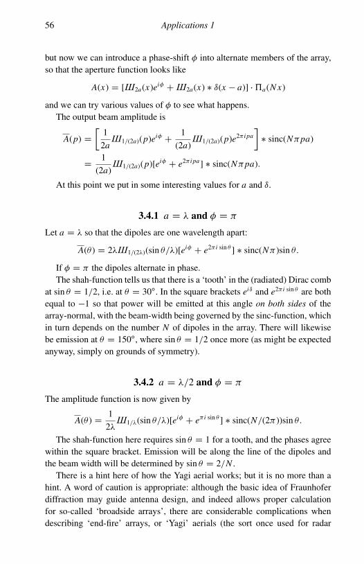
56 Applications 1
but now we can introduce a phase-shift φ into alternate members of the array,so that the aperture function looks like
A(x) D [Ш2a(x)eiφ CШ2a(x) � δ(x � a)] ��a(Nx)
and we can try various values of φ to see what happens.The output beam amplitude is
A(p) D
[1
2aШ1/(2a)(p)eiφ C
1
(2a)Ш1/(2a)(p)e2πipa
]� sinc(Nπpa)
D1
(2a)Ш1/(2a)(p)[eiφ C e2πipa] � sinc(Nπpa).
At this point we put in some interesting values for a and δ.
3.4.1 a D λ and φ D π
Let a D λ so that the dipoles are one wavelength apart:
A(θ ) D 2λШ1/(2λ)(sin θ/λ)[eiφ C e2πi sin θ ] � sinc(Nπ )sin θ.
If φ D π the dipoles alternate in phase.The shah-function tells us that there is a ‘tooth’ in the (radiated) Dirac comb
at sin θ D 1/2, i.e. at θ D 30ı. In the square brackets eiδ and e2πi sin θ are bothequal to �1 so that power will be emitted at this angle on both sides of thearray-normal, with the beam-width being governed by the sinc-function, whichin turn depends on the number N of dipoles in the array. There will likewisebe emission at θ D 150ı, where sin θ D 1/2 once more (as might be expectedanyway, simply on grounds of symmetry).
3.4.2 a D λ/2 and φ D π
The amplitude function is now given by
A(θ ) D1
2λШ1/λ(sin θ/λ)[eiφ C eπi sin θ ] � sinc(N/(2π ))sin θ.
The shah-function here requires sin θ D 1 for a tooth, and the phases agreewithin the square bracket. Emission will be along the line of the dipoles andthe beam width will be determined by sin θ D 2/N .
There is a hint here of how the Yagi aerial works; but it is no more than ahint. A word of caution is appropriate: although the basic idea of Fraunhoferdiffraction may guide antenna design, and indeed allows proper calculationfor so-called ‘broadside arrays’, there are considerable complications whendescribing ‘end-fire’ arrays, or ‘Yagi’ aerials (the sort once used for radar

3.4 Dipole arrays 57
transmission and television reception). The broadside array, which comprisesa number of dipoles (each dipole consisting of two rods, lying along the sameline, each λ/4 long and with an alternating voltage applied in the middle),behaves like a row of point sources of radiation, and the amplitude at dis-tances large compared with a wavelength can be calculated. Both the amplitudeand the relative phase radiated by each dipole can be controlled7 so that theshape of the radiation pattern and the strengths of the side-lobes are undercontrol.
End-fire antennae, on the other hand, have one dipole driven by an oscillatorand rely on resonant oscillation of the other ‘passive’ dipoles to interfere withthe radiation pattern and direct the output power in one direction. The nearestoptical analogue is probably the Fabry–Perot etalon or, which is practically thesame thing, the interference filter. The phase re-radiated by a passive dipoledepends on whether it is really half a wavelength long, on its conductivity, whichis not perfect, and on the dielectric constant of any sheath which may surroundit. Consequently, aerial design tends to be based on experience, experimentand computation, rather than on strict Fraunhofer theory. The passive elementsmay be λ/3 apart, for example, and their lengths will taper along the directionof the aerial, being slightly shorter on the transmission side and longer on thereflecting side of the excited dipole. Spacings are non-uniform, sometimes withthe spacing changing logarithmically or exponentially, with some elementsof peculiar shape, some ‘folded’, some ‘batwinged’ – and so it goes.8 Suchmodifications allow a broader band of radiation to be transmitted or receivedalong a narrow cone possibly only a few degrees wide. Aerial design is a blackart, a path bestrewn with empiricism, with Christmas-tree designs of weirdcomplexity and with patent-infringement law-suits.
3.4.3 To continue . . .
At this point the reader’s curiosity may take up the challenge. For instance theamplitude function may be split into three or more components. For example,
A(x) D[Ш3a(x)eiφ1 CШ3a(x)eiφ2 � δ(x � a)
CШ3a(x)eiφ3 � δ(x � 2a)]��a(Nx)
so that a different phase shift is applied to every third aerial.So far we have considered Dirac combs with uniform spacing between the
teeth. The door is wide open for the exploration of the convolution algebra of
7 This is equivalent to apodizing in optics, but with more flexibility.8 To paraphrase Vonnegut.

58 Applications 1
Fig. 3.14. The polar diagram of a sinc2-function.
delta-function combs with unequal spacing, which may be logarithmic, arith-metic, exponential, Fibonacci and so on, all possibly yielding deeper insightsinto the black art mentioned above.
3.5 Polar diagrams
Since the important feature of Fraunhofer theory is the angle of diffraction, itis sometimes more useful, especially in antenna theory, to draw the intensitypattern on a polar diagram, with intensity as r , the length of the radius vector,and θ as the azimuth angle. The sinc2-function then appears as in Fig. 3.14.Sometimes the logarithm of the intensity is plotted instead, to give the gain ofthe antenna as a function of angle.
3.6 Phase and coherence
Coherence is an important concept, not only in optics, but whenever oscillatorsare compared.
No natural light source is exactly monochromatic, and there are small varia-tions in period and hence wavelength from time to time. Two sources are said tobe coherent when any small variation in one is matched by a similar variationin the other, so that, for example, if a crest of a wave from one arrives at agiven point at the same instant as the trough of a wave from the other, then atall subsequent times troughs and crests will arrive together and there is alwaysdestructive interference between the two.
3.6 Phase and coherence 59
In practice the variations of wavelength and phase in a quasi-monochromaticsource are slow and if the wave train is divided – for example by a beam-splitter, then one wave train will be almost coherent with the other whichhas been delayed by a few wavelengths, as happens in an interferometer. Asthe path-difference is increased, by moving one of the interferometer mirrors,the fringes become less and less distinct and if the path-difference is greatenough they vanish. We have reached the limit of coherence and can referto the coherence length of the wave train. In ‘allowed’ (i.e. dipole) atomictransitions, for example, each individual wave train has a coherence length ofa few metres, corresponding to the time taken for the atom to emit its light.In a laser, where the emitted light is in phase with the stimulating light, thecoherence length may be anything up to a hundred times as long as the lasercavity,9 the length depending on the reflectivity of the laser mirrors. The linewidth is correspondingly narrow, much narrower than the ‘natural’ width of thelight emitted by the gas in the cavity. Similarly one can imagine the coherenceof light from a distant extended source, where no source element is coherentwith any other element. In this case, when light passes through a narrow slit, thewave trains arriving at one edge of the slit will sum to a complicated function oftime, but, if the paths to the other edge of the slit all differ from the first set byless than a few wavelengths, the function of time there will be almost the sameas for the first set and all the wave trains passing through the slit will interfereas if the source were coherent. You can hold close to your eye a spectroscopeslit open a few microns, and look at a distant bright extended source such asa frosted light-bulb: it will show the secondary maxima of the sinc2-functionwhich would be produced if all the source-elements in the bulb were coherent.If the slit is opened slowly, the secondary maxima will crowd in to the principalmaximum and eventually disappear.
In this case we refer to the slit width as the coherence width of the source –it is a property of the source, not of the equipment used to view it. If theexperiment is done in two orthogonal directions the coherence area of thesource can be measured.
The coherence width of the sun in green (λ D 550 nm) light, for example, isabout 60 µm, and with a narrow-band interference filter over the slit (to avoideye-damage!) the familiar sinc2 pattern can be seen with the slit opened to aboutthis width. It is no coincidence of course that plane monochromatic wavefrontsincident on and diffracted through the same slit will show a principal maximumin their diffraction pattern of the same angular width as the extended source.
9 Sometimes much greater. See J. L. Hall’s 2005 Nobel Prize lecture, J. L. Hall, Rev. Mod. Phys.78 (2006), 1279–1295.

60 Applications 1
Fig. 3.15. The vector addition of two analytic wave-vectors representing twocoherent sources. All three vectors are rotating at the same frequency ν. Thethree vectors are described by complex numbers of the form Ae2πiνt , the so-called ‘analytic signal’, but it is the real part of each, the horizontal componentin the graph, which represents the instantaneous value of the electric field of thelight-wave.
A star, on the other hand, has a coherence width of many – perhaps tens orhundreds – of metres and a Young’s-slit interferometer with the apertures spacedby this sort of distance will show interference fringes, with the fringe visibilityfalling slowly as the distance between the apertures is increased. Michelsonused this effect to measure the coherence width and hence the angular diameterof several stars.
3.7 Fringe visibility
An alternative way of describing coherence is by considering the analytic wave-vectors on the Argand plane, which rotate at about 6 � 1014 Hz for green light,but which, for two coherent sources, are rigidly linked by the phase-differencebetween them. If we abandon the time variation, the vector diagram looks likeFig. 3.15 and the resultant amplitude is the vector sum of the components.The resultant amplitude may be zero if the two sources are perfectly coherent,of equal amplitude and opposite in phase. Otherwise the resultant intensity isproportional to the square of the length of this vector.
If the sources are only partially coherent (Fig. 3.16) it means that the ampli-tude and phase angles are varying randomly over angles small compared with2π . Interference fringes from such a pair of sources will show an intensitypattern on a screen given by
I D I1 C I2 C 2�12
√I1I2 cos φ,

3.8 The Michelson stellar interferometer 61
a
b
c
imaginaryaxis
real axis
Fig. 3.16. The analytic vector diagram for two quasi-coherent sources. The twovectors here are varying randomly only in phase. Nevertheless, the resultant vectorvaries both in phase and in amplitude, and wanders randomly within the generalarea of the quadrilateral. Even if the amplitudes were the same and the phasesopposed, there would not be complete cancellation.
where �12 is known as the degree of coherence, the coherence factor or thecoefficient of coherence. �12 is always �1.
As usual, φ is the phase difference, which varies from place to place on thediffraction pattern.
The maximum intensity Imax in the pattern is at places where φ D 2nπ and isgiven by Imax D I1 C I2 C �12. The minimum intensity, where φ D (2nC 1)π ,is Imin D I1 C I2 � �12.
We can now define the visibility, V , of the fringe pattern by
V D (Imax � Imin)/(Imax C Imin)
and clearly, provided that the two sources are of equal intensity, V D �12.
3.8 The Michelson stellar interferometer
This is essentially a Young’s-slit interferometer on an heroic scale. The aper-tures are two mirrors mounted on carriages which run along a beam fixed to theupper end of an astronomical reflecting telescope and they reflect light from abright star to two more mirrors fixed near the centre of the beam, which in turndirect the light to the telescope objective and hence to the focus. At high magni-fication, interference fringes can be seen in the eyepiece, superimposed on the

62 Applications 1
w
I (a)
q aq
Fig. 3.17. Young’s-slit interferometry with a distant extended source. An elementof the source coming from a direction making an angle θ with the optic axis willproduce its own infinitesimal fringe pattern displaced by this angle θ . All thesefringe patterns, incoherent with each other, have their intensities added to form theresultant fringe pattern of lower visibility.
(large!) diffraction-limited image of the star. Atmospheric turbulence causesthe image to move and shimmer, but the fringes move with the stellar imageand remain visible to the observer. The visibility of the fringes diminishes asthe mirror separation increases and may fall to zero at some point.
We now demonstrate that the fringe visibility, measured as a functionof the mirror separation, is the modular Fourier transform of the
intensity distribution across the source.
In Fig. 3.17, a distant, monochromatic point source of intensity S(0) lying onthe optic axis will give fringes and the intensity will vary sinusoidally accordingto
I (α) D S(0)
[1C cos
(2π
λw cos α
)],
where λ is the wavelength, w the slit separation and α the angular variabledescribing the fringe pattern. The period of the pattern is λ/w, and depends onthe slit separation, w.
This, of course, is a standard result in physical optics.

3.8 The Michelson stellar interferometer 63
Another such source, situated at an angle θ to the optic axis, similarlyproduces perfect10 fringes but displaced sideways by the same angle θ on thefringe pattern. The two sources are incoherent, so if they are both present theirintensities are added.
If instead there is an extended distant source with intensity varying as S(θ ),an element of infinitesimal intensity S(θ )dθ will produce its own infinitesimalfringe pattern in the interferometer, displaced sideways by θ .
All these separate fringe patterns must be summed, so that the resultantintensity emerging at angle α to form the fringe pattern will be
I (α) D∫ 1
�1
S(θ )dθ
[1C cos
(2π
λw(α � θ )
)],
which separates to
I (α) D∫ 1
�1
S(θ )dθ C
∫ 1
�1
S(θ )
[cos
(2π
λw(α � θ )
)]dθ,
where the sines of the small angles α and θ have been replaced by the anglesthemselves.
The first term represents the total intensity coming from the extended source.The second term is the convolution of the source intensity distribution S(θ ) withthe cosine, which we write as C(α),
C(α) D S(θ ) � cos(2πpθ ),
and the variable p, conjugate to α, is w/λ.The convolution integral, nominally from �1 to C1, is in practice over
the angular width of the source.The result of the convolution, as we saw11 in Chapter 2, is a sinusoid with
period 1/p, determined by the wavelength λ and the (adjustable) distancew between the two apertures. It has an amplitude A(p), the amplitude ofthe corresponding Fourier component in the transform of the source intensitydistribution. (Bear in mind that in the Fourier transform the variable conjugateto α is p, and A(p)• S(α).) The intensity maxima of the resultant fringepattern are S C A and the minima are S � A so that the fringe visibility, as afunction of p, that is, of w/λ, is
V DA(w/λ)
S(3.3)
and A(w/λ) is the Fourier transform of S(θ ). This is demonstrated in Fig. 3.18.
10 That is, of visibility V D 1. 11 On p. 38.

64 Applications 1
d (p + w/l) d (p – w/l) p
A(p)
S
Fig. 3.18. The fringe visibility as a function of w/λ.
The fringe visibility thus decreases as w increases. When stellar diameterswere measured it was a reasonable assumption that S(θ ) was symmetrical sothat its Fourier transform was real and symmetrical.
Otherwise A(w/λ) was the modular transform, as for example when observ-ing a double-star with components of unequal intensity, but in practice the pointwas academic, since phase-shifts in the fringe pattern would anyway be lostin the atmospheric disturbance, and it is simply the minima or vanishing ofthe fringes that were observed at particular values of w. If, for example, adouble star with two equal components were observed, S(θ ) would be a pairof δ-functions and the fringe visibility as a function of w/λ would decreasesinusoidally to zero, then increase again in inverse phase. The value of w atzero visibility would be observable but the phase inversion would not.
3.9 The van Cittert–Zernike theorem
The original Michelson stellar interferometer12 comprised two 150-mm-diameter plane mirrors mounted with their normals at 45ı to the optic axisof the 10000 Hooker telescope at the Mount Wilson observatory. To vary w,they could be moved on trolleys along a 6-m-long girder fixed to the top ofthe telescope tube, and the light from them was directed to two fixed mirrorsalso at 45ı, whence the light was passed through to the telescope objectiveand hence to the focus. The Young ‘slits’ were thus the two moveable mirrorson the girder, which reflected starlight13 from a star or perhaps a double star.The point of this description is that the orientation of the two apertures couldhave been altered and, if the star had had an ellipsoidal shape, for example,
12 A. A. Michelson and F. G. Pease, Astrophys. J. 53 (1921), 249.13 In fact they began with the red giant Betelgeuse, also known as α-Orionis.

3.9 The van Cittert–Zernike theorem 65
the coherence width would have been greater when the apertures were alignedwith the star’s minor axis. The fringe visibility would measure the degree ofcoherence for that particular separation and that particular orientation. A shape,called the ‘coherence area’ of the star, could in principle be mapped out, and thevan Cittert–Zernike theorem, in its crudest form, states that the fringe visibility,i.e. the degree of coherence, as a function of w and the orientation angle ξ , isthe two-dimensional Fourier transform of the intensity distribution on the skyas a function of α and ξ .
Thus, in its most elementary – and practical – form, the van Cittert–Zerniketheorem is described by equation (3.3) above.
This is not the place for a full rigorous derivation and proof of the theoremwhich considers the complex degree of coherence (as exemplified by the phase-shift of the fringes) and which occupies two pages in Born & Wolf’s Principlesof Optics.14 The idea of a ‘coherence area’ is the important thing. It is not fixedin space (the telescope is moving both with Earth’s orbital speed and with thediurnal rotational speed of the Mount Wilson observatory) but is measured bythe separation of the two apertures. It is the ‘area over which some degree ofcoherence can be observed’.
To put it another way: if there were a circular coherent source of monochro-matic light of the diameter and at the distance of Betelgeuse its ‘Airy disc’ hereon Earth would have a diameter of about 6 m.
14 M. Born and E. Wolf, Principles of Optics, Cambridge University Press, Cambridge, 7th edn,1999, pp. 572–574.

4
communication theory
4.1 Communication channels
Although the concepts involved in communication theory are general enoughto include bush-telegraph drums, alpine yodelling or a ship’s semaphore flags,by ‘communication channel’ is usually meant a single electrical conductor,a waveguide, a fibre-optic cable or a radio-frequency carrier wave. Commu-nication theory covers the same general ground as information theory, whichdiscusses the ‘coding’ of messages (such as Morse code, not to be confused withencryption, which is what spies do) so that they can be transmitted efficiently.Here we are concerned with the physical transmission, by electric currentsor radio waves, of the signal or message that has already been encoded. Thedistinction is that communication is essentially an analogue process, whereasinformation coding is essentially digital.
For the sake of argument, consider an electrical conductor along which issent a varying current, sufficient to produce a potential difference V (t) acrossa terminating impedance of one ohm (1�).
The mean level or time-average of this potential is denoted by the symbolhV (t)i defined by the equation:
hV (t)i D1
2T
∫ T
�T
V (t)dt.
The power delivered by the signal varies from moment to moment, and it toohas a mean value:
hV 2(t)i D1
2T
∫ T
�T
V 2(t)dt.
For convenience, signals are represented by functions like sinusoids which, ingeneral, disobey one of the Dirichlet conditions described at the beginning of
66
Applications 2: signal analysis and

4.1 Communication channels 67
Chapter 2: they are not square-integrable:
limT !1
∫ T
�T
V 2(t)dt !1.
However, in practice, the signal begins and ends at finite times and we regardthe signal as the product of V (t) with a very broad top-hat function. Its Fouriertransform – which tells us about its frequency content – is then the convolutionof the true frequency content with a sinc-function so narrow that it can for mostpurposes be ignored. We thus assume that V (t)! 0 at jt j > T and that∫ 1
�1
V 2(t)dt D
∫ T
�T
V 2(t)dt.
We now define a function C(ν) such that C(ν)• V (t), and Rayleigh’s theoremgives ∫ 1
�1
jC(ν)j2 dν D
∫ 1
�1
V 2(t)dt D
∫ T
�T
V 2(t)dt.
The mean power level in the signal is then
1
2T
∫ T
�T
jV (t)j2 dt
since V 2(t) is the power delivered into unit impedance; and then
1
2T
∫ T
�T
jV (t)j2 dt D
∫ 1
�1
jC(ν)j2
2Tdν
and we define jC(ν)j2/(2T ) D G(ν) to be the spectral power density (SPD) ofthe signal.
4.1.1 The Wiener–Khinchine theorem
The autocorrelation function of V (t) is defined to be
limT !1
1
2T
∫ T
�T
V (t)V (t C τ )dt D hV (t)V (t C τ )i.
Again the integral on the left-hand side diverges and we use the shift theoremand Parseval’s theorem to give∫ T
�T
V (t)V (t C τ )dt D
∫ 1
�1
C�(ν)C(ν)e2πiντ dν.

68 Applications 2
Then
1
2T
∫ T
�T
V (t)V (t C τ )dt D
∫ 1
�1
jC(ν)j2
2Te2πiντ dν D R(τ )
so that, with the definition of G(ν) above,
R(τ ) D∫ 1
�1
G(ν)e2πiντ dν
and finally
R(τ )• G(ν).
In other words,
the spectral power density is the Fourier transform of theautocorrelation function of the signal.
This is the Wiener–Khinchine theorem.
4.2 Noise
The term originally meant the random fluctuation of signal voltage which washeard as a hissing sound in early telephone receivers, and which is still heard inradio receivers which are not tuned to a transmitting frequency. Now it is takento mean any randomly fluctuating signal which carries no message or ‘informa-tion’. If it has equal power density at all frequencies it is called ‘white’ noise.1
Its autocorrelation function is always zero since at any time the signal n(t),being random, is as likely to be negative as to be positive. The only exception isat zero delay, τ D 0, where the integral diverges. The autocorrelation functionis therefore a δ-function and its Fourier transform is unity, in accordance withthe Wiener–Khinchine theorem and with this definition of ‘white’.
In practice the band of frequencies which is received is always finite, sothat the noise power is always finite. There are other types of noise, forexample:
� Electron shot noise, or ‘Johnson noise’, in a resistor, giving a random fluctua-tion of voltage across it: hV 2(t)i D 4πRkT ν, where ν is the bandwidth,R the resistance, k Boltzmann’s constant and T the absolute temperature.2
1 This is a rebarbative use of ‘white’, which really defines a rough surface which reflects all theradiation incident upon it. It is used, less compellingly, to describe the colour of the lightemitted by the Sun or, even less compellingly, to describe light of constant spectral powerdensity in which all wavelengths (or frequencies; take your pick) contribute equal power.
2 hV 2i D 1.3 � 10�10(R ν)1/2 volts in practice.

4.3 Filters 69
� Photo-electron shot noise, which has a normal (Gaussian) distribution ofcount-rate3 at frequencies low compared with the average generation-rateand, more accurately, a Poisson distribution when equal time-samples aretaken. This kind of noise is met chiefly in fibre optics when light is usedfor communication, and only then when the light is weak. Typically, a laserbeam delivers 1018 photons s�1, so that even at 100 MHz there are 1010
photons/sample, or an S/N ratio of 105 : 1.� Semiconductor noise, which gives a time-varying voltage with a spectral
power density which varies as 1/ν – which is why many semiconductordetectors of radiation are best operated at high frequency with a ‘chopper’ toswitch the radiation on and off. There is usually an optimum frequency, sincethe number of photons in a short sample may be small enough to increasephoton shot noise to the level of the semiconductor noise.
4.3 Filters
By ‘filter’ we mean an electrical impedance which depends on the frequencyof the signal current trying to pass. The exact structure of the filter, namelythe arrangement of resistors, capacitors and inductances, is immaterial. Whatmatters is the effect that the filter has on a signal of fixed frequency and unitamplitude. The filter does two things: it attenuates the amplitude and it shiftsthe phase. This is all that it does.4 The frequency-dependence of its impedanceis described by its filter function Z(ν). This is defined to be the ratio of theoutput voltage divided by the input voltage, as a function of frequency:
Z(ν) D Vo/Vi D A(ν)eiφ(ν),
where Vi and Vo are ‘analytic’ representations of the input and output voltages,i.e. they include the phase as well as the amplitude. The impedance is complexsince both the amplitude and the phase of Vo may be different from thoseof Vi. The filter impedance, Z, is usually shown graphically by plotting apolar diagram of the attenuation, A, radially against the angle of phase-shift,eliminating ν as a variable. The result is called a Nyquist diagram (Fig. 4.1).This is the same figure as that which is used to describe a feedback loop inservo-mechanism theory, with the difference that the amplitude A is always lessthan unity in a passive filter, so that there is no fear of the curve encompassingthe point (�1, 0), the criterion for oscillation in a servo-mechanism.
3 Which may be converted into a time-varying voltage by a rate-meter.4 Unless it is ‘active’. Active filters can do other things, such as doubling the frequency of the
input signal.
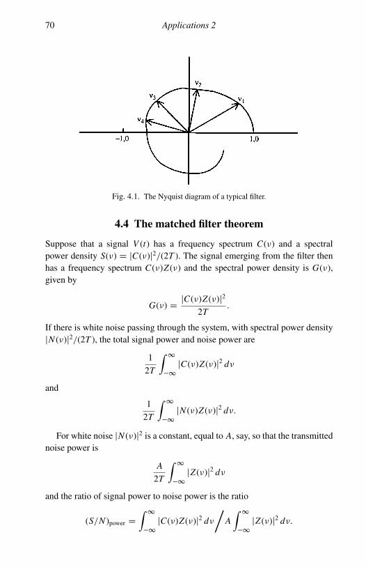
70 Applications 2
Fig. 4.1. The Nyquist diagram of a typical filter.
4.4 The matched filter theorem
Suppose that a signal V (t) has a frequency spectrum C(ν) and a spectralpower density S(ν) D jC(ν)j2/(2T ). The signal emerging from the filter thenhas a frequency spectrum C(ν)Z(ν) and the spectral power density is G(ν),given by
G(ν) DjC(ν)Z(ν)j2
2T.
If there is white noise passing through the system, with spectral power densityjN (ν)j2/(2T ), the total signal power and noise power are
1
2T
∫ 1
�1
jC(ν)Z(ν)j2 dν
and
1
2T
∫ 1
�1
jN (ν)Z(ν)j2 dν.
For white noise jN (ν)j2 is a constant, equal to A, say, so that the transmittednoise power is
A
2T
∫ 1
�1
jZ(ν)j2 dν
and the ratio of signal power to noise power is the ratio
(S/N )power D
∫ 1
�1
jC(ν)Z(ν)j2 dν
/A
∫ 1
�1
jZ(ν)j2 dν.
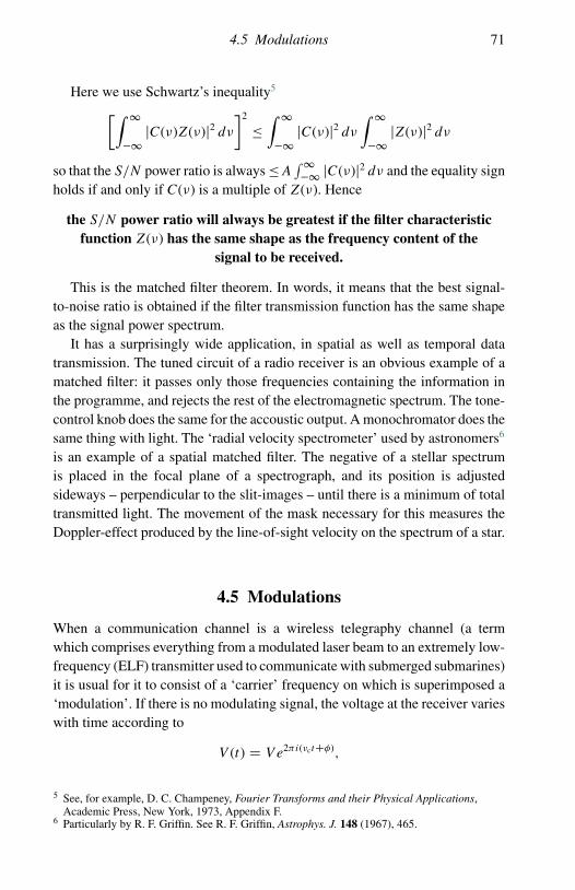
4.5 Modulations 71
Here we use Schwartz’s inequality5
[∫ 1
�1
jC(ν)Z(ν)j2 dν
]2
�
∫ 1
�1
jC(ν)j2 dν
∫ 1
�1
jZ(ν)j2 dν
so that the S/N power ratio is always�A∫1
�1 jC(ν)j2 dν and the equality signholds if and only if C(ν) is a multiple of Z(ν). Hence
the S/N power ratio will always be greatest if the filter characteristicfunction Z(ν) has the same shape as the frequency content of the
signal to be received.
This is the matched filter theorem. In words, it means that the best signal-to-noise ratio is obtained if the filter transmission function has the same shapeas the signal power spectrum.
It has a surprisingly wide application, in spatial as well as temporal datatransmission. The tuned circuit of a radio receiver is an obvious example of amatched filter: it passes only those frequencies containing the information inthe programme, and rejects the rest of the electromagnetic spectrum. The tone-control knob does the same for the accoustic output. A monochromator does thesame thing with light. The ‘radial velocity spectrometer’ used by astronomers6
is an example of a spatial matched filter. The negative of a stellar spectrumis placed in the focal plane of a spectrograph, and its position is adjustedsideways – perpendicular to the slit-images – until there is a minimum of totaltransmitted light. The movement of the mask necessary for this measures theDoppler-effect produced by the line-of-sight velocity on the spectrum of a star.
4.5 Modulations
When a communication channel is a wireless telegraphy channel (a termwhich comprises everything from a modulated laser beam to an extremely low-frequency (ELF) transmitter used to communicate with submerged submarines)it is usual for it to consist of a ‘carrier’ frequency on which is superimposed a‘modulation’. If there is no modulating signal, the voltage at the receiver varieswith time according to
V (t) D V e2πi(νctCφ),
5 See, for example, D. C. Champeney, Fourier Transforms and their Physical Applications,Academic Press, New York, 1973, Appendix F.
6 Particularly by R. F. Griffin. See R. F. Griffin, Astrophys. J. 148 (1967), 465.

72 Applications 2
Fig. 4.2. A carrier wave with amplitude modulation.
vc − nmod nc + nmodncn
A(n)
Fig. 4.3. Various modulating frequencies occupy a band of the spectrum. The timefunction is A C B cos(2πνmodt) and in frequency space the spectrum becomes theconvolution of δ(ν � νc) with Aδ(ν) C B[(δ(ν � νmod) C δ(ν C νmod)]/2.
where νc is the carrier frequency; and the modulation may be carried out bymaking V , νc or φ a function of time.
� Amplitude modulation (Fig. 4.3). If V varies with a modulating frequencyνmod, then V D AC B cos(2πνmodt) and the resulting frequency distributionwill be as in Fig. 4.2 and, as various modulating frequencies from 0! νmax
are transmitted, the frequency spectrum will occupy a band of the spectrumfrom νc � νmax to νc C νmax. If low modulating frequencies predominate inthe signal, the band of frequencies occupied by the channel will have theappearance of Fig. 4.3 and the filter in the receiver should have this profiletoo.
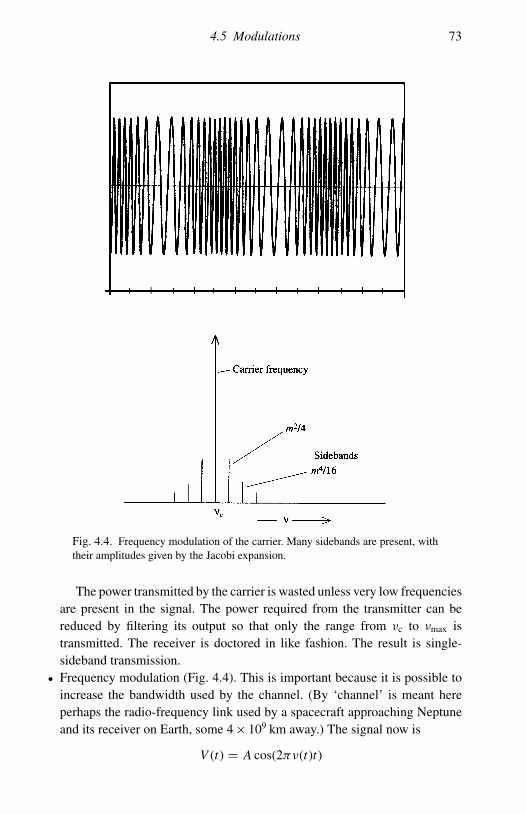
4.5 Modulations 73
Fig. 4.4. Frequency modulation of the carrier. Many sidebands are present, withtheir amplitudes given by the Jacobi expansion.
The power transmitted by the carrier is wasted unless very low frequenciesare present in the signal. The power required from the transmitter can bereduced by filtering its output so that only the range from νc to νmax istransmitted. The receiver is doctored in like fashion. The result is single-sideband transmission.
� Frequency modulation (Fig. 4.4). This is important because it is possible toincrease the bandwidth used by the channel. (By ‘channel’ is meant hereperhaps the radio-frequency link used by a spacecraft approaching Neptuneand its receiver on Earth, some 4 � 109 km away.) The signal now is
V (t) D A cos(2πν(t)t)

74 Applications 2
and ν(t) itself is varying according to ν(t) D νcarrier C µ cos(2πνmod(t)t).The parameter µ can be made very large so that, for example, a voicetelephone signal normally requiring about 3 � 103 Hz bandwidth can be madeto occupy several MHz if necessary. The advantage in doing this is foundin the Hartley–Shannon theorem of information theory, which states that the‘channel capacity’, the rate at which a noisy channel can transmit informationin bits s�1 (‘bauds’), is given by
dB/dt � 2� loge(1C S/N ),
where � is the channel bandwidth, S/N is the power signal-to-noise ratioand dB/dt is the ‘baud-rate’ or bit-transmission rate.
So, to get a high data transmission rate, you need not slave to improve theS/N ratio because only the logarithm of that is involved: instead you increasethe bandwidth of the transmission. In this way the low power available tothe spacecraft transmitter near Neptune is used more effectively than wouldbe possible in an amplitude-modulated transmitter. Theorems in informationtheory, like those in thermodynamics, tend to tell you what is possible, withouttelling you how to do it.
To see how the power is distributed in a frequency-modulated carrier, themessage-signal, a(t), can be written in terms of the phase of the carrier signal,bearing in mind that frequency can be defined as rate of change of phase. Ifthe phase is taken to be zero at time t D 0, then the phase at time t can bewritten as
φ D
∫ t
0
∂φ
∂tdt
and ∂φ/∂t D νc C∫ t
0 a(t)dt and the transmitted signal is
V (t) D ae2πi
[νcC
∫ t
0 a(t)dt
]t.
Consider a single modulating frequency νmod, such that a(t) Dk cos(2πνmodt). Then
2πi
∫ t
0a(t)dt D
2πik
2πνmodsin(2πνmodt),
where k is the depth of modulation, and k/νmod is called the modulationindex, m. Then
V (t) D Ae2πiνct eim sin(2πνmodt).
It is a cardinal rule in applied mathematics that, when you see an exponentialfunction with a sine or cosine in the exponent, there is a Bessel function

4.5 Modulations 75
lurking somewhere. This is no exception. The second factor in the expressionfor V (t) can be expanded in a series of Bessel functions by the Jacobiexpansion7
eim sin(2πνmodt) D
1∑nD�1
Jn(m)e2πinνmodt
and this is easily Fourier transformable to
χ (ν) D1∑
nD�1
Jn(m)δ(ν � nνmod).
The spectrum of the transmitted signal is the convolution of χ (ν) with δ(ν �νc). In other words, χ (ν) is shifted sideways so that the n D 0 tooth of theDirac comb is at ν D νc.
The amplitudes of the Bessel functions must be computed or looked up ina table8 and for small values of the argument m are J0(m) D 1, J1(m) D m/2,J2(m) D m2/4 etc. Each of these Bessel functions multiplies a correspondingtooth in the Dirac comb of period νmod to give the spectrum of the modulatedcarrier. Bearing in mind that m D k/νmod, we see that the channel is notuniformly filled and there is less power in higher frequencies.
As an example of the cross-fertilizing effect of Fourier transforms, thetheory above can equally be applied to the diffraction produced by a gratingin which there is a periodic error in the rulings. In Chapter 3 there was anexpression for the ‘aperture function’ of a grating, which was
A(x) D �Na(x)[�a(x) �Шa(x)],
and if there is a periodic error in the ruling, it is Шa(x) that must be replaced.The rulings, which should have been at x D 0, a, 2a, 3a, . . . , will beat 0, a C α sin(2πβ � a), 2a C α sin(2πβ � 2a), . . . etc. and the Ш-functionis replaced by
G(x) D1∑
�1
δ[x � na � α sin(2πβna)],
where α is the amplitude of the periodic error and 1/β is its ‘pitch’. This hasa Fourier transform
G(p) D1∑
�1
e2πi[naCα sin(2πβna)]
7 See, for example, H. Jeffreys & B. Jeffreys, Methods of Mathematical Physics, 3rd edn,Cambridge University Press, Cambridge, 1999, p. 589.
8 For example, in Jahnke & Emde or Abramowitz & Stegun (see the bibliography).

76 Applications 2
Fig. 4.5. Rowland ghosts in the spectrum produced by a diffraction grating witha period error in its rulings. The spacing of the ghost from its parent line dependson the period of the error, and the intensity depends on the square of the amplitudeof the error.
with p D sin θ/λ as in Chapter 3. There is a clear analogy with V (t) above.The diffraction pattern then contains what are called ‘ghost’ lines9 aroundeach genuine spectrum line as in Fig. 4.5.
The analysis is not quite as simple as in the case of a frequency-modulatedradio wave because the simple sinusoids are replaced by δ-functions. Whathappens is that the infinite sum G(p) can be analysed into a whole set of Diraccombs, of periods slightly above and below the true error-free period, andwith amplitudes decreasing rapidly according to the amplitude of the Besselfunction which multiplies them. The Rowland ghosts are then separatedfrom the parent line by distances which depend on the pitch 1/β of the lead-screw of the grating ruling engine and have amplitudes which depend on thesquare10 of the amplitude α of the periodic error.
These satellites on either side of a spectrum line with intensity π2p2α2
times the height of the parent and separated from it by λ D ˙aβλ arethe first-order Rowland ghosts. The next ones, of height π4p4α4 timesthe parent intensity, are the second-order ghosts, and so on. The anal-ogy with the channel occupation of a frequency-modulated carrier isexact.
There are, of course, many other ways of modulating a carrier, such as phasemodulation, pulse-width modulation, pulse-position modulation, pulse-heightmodulation and so on, quite apart from digital encoding, which is a quiteseparate way of conveying information. Several different kinds of modulationcan be applied simultaneously to the same carrier, each requiring a differ-ent type of demodulating circuit at the receiver. The design of communica-tions channels includes the art of combining and separating these modulators
9 Rowland ghosts, after H. A. Rowland, the inventor of the first effective grating-ruling engine.10 Because G(p) gives the diffraction amplitude.

4.7 Passage of signals through simple filters 77
and ensuring that they do not influence each other with various kinds of‘cross-talk’.
4.6 Multiplex transmission along a channel
There are two ways of sending a number of independent signals along the samecommunication channel. They are known as time-multiplexing and frequency-multiplexing. Frequency multiplexing is the more commonly used. The sig-nals to be sent are used to modulate11 a sub-carrier, which then modulatesthe main carrier. A filter at the receiving end demodulates the main carrierand transmits only the sub-carrier and its sidebands (which contain the mes-sage). Different sub-carriers require different filters and it is usual to leave asmall gap in the frequency spectrum between sub-carriers in order to guardagainst ‘cross-talk’, that is one signal spreading into the pass-band of anothersignal.
Time-multiplexing involves the ‘sampling’ of the carrier at regular timeintervals. If, for example, there are ten separate signals to be sent, the sam-pling rate must be twenty times the highest frequency present in each band.The samples are sent in sequence and switched to ten different channels fordecoding, and there must be some way of collating each message channel atthe transmitting end with its counterpart at the receiving end so that the rightmessage goes to the right recipient. The ‘serial link’ between a computer anda peripheral, which uses only one wire, is an example of this, with about eightchannels,12 one for each bit-position in each byte of data.
4.7 The passage of some signals through simple filters
This is not a comprehensive treatment of the subject, but illustrates the methodsused to solve problems. Firstly we need to know about the Heaviside step-function.
4.7.1 The Heaviside step-function
When a switch is closed in an electric circuit there is a virtually instanta-neous change of voltage on one side. This can be represented by a ‘Heaviside
11 ‘Modulate’ here means that the main carrier signal is multiplied by the message-bearingsub-carrier. Demodulation is the reverse process, in which the sub-carrier and its message areextracted from the transmitted signal by one of various electronic tricks.
12 Anything between five and eleven channels in practice, so long as the transmitter and receiverhave agreed beforehand about the number.

78 Applications 2
0 t
Fig. 4.6. An analytic function approximating to a Heaviside step-function in thelimit a ! 0.
step-function’, H (t). It has the property that H (t) D 0 for t < 0 and H (t) D 1for t > 0.13 Like the delta-function, it can be represented as the limit of ananalytic function (Fig. 4.6), for example
H (t) D lima!0
[1
1C e�2t/a
],
which tends to unity as t tends to 1, tends to zero as t tends to �1 andautomatically takes the value 1/2 at t D 0.
However, this function is not Fourier-transformable because it does notsatisfy the Dirichlet condition of being square-integrable.
Instead we construct a function as follows.We begin with the so-called ‘sgn’-function (Fig. 4.7), defined by
sgn(t) D
{�1, �1 < t < 0,
C1, 0 < t <1
and we divide it by 2 and add 1/2 to give a Heaviside step of unit height.The function sgn(t)/2 likewise does not obey the Dirichlet conditions but
can be approximated in several ways. It may be regarded, for example, as thelimiting case of a pair of ‘ramp’ functions, defined by
f (t) D
lima!0
�(at C 1)
2, �1/a < x < 0,
lima!0
(1 � at)
2, 0 < x < 1/a
and the functions of this pair obey the Dirichlet conditions (at least before we goto the limit!), and together form an antisymmetrical function which, as a ! 0,
13 Its value at x D 0 is the subject of debate, but is usually taken as H (0) D 1/2.

4.7 Passage of signals through simple filters 79
0, 1
0, –1
Fig. 4.7. The sgn function sgn(t).
0, – 12
0,
, 0a
, 0
–1
12
1a
Fig. 4.8. Representation of a Heaviside step-function by two functions whichobey the Dirichlet conditions.
approaches sgn(t)/2. As it does so those parts of its Fourier transform whichhave a factor a all vanish, leaving us with the Fourier transform of sgn(t)/2.Adding 1/2 to give the step function means that we add δ(ν)/2 to the Fouriertransform of sgn(t)/2. (See Fig. 4.8.)
The sum of the Fourier transforms14 of these three components in the limitas a ! 0 is
φ(ν) Dδ(ν)
2C
1
2πiν.
For all practical purposes we can ignore the δ-function since it cancels itselfout when any finite limits appear in the Fourier transform.
14 Remember to do the inverse transform, with �2πiνt in the exponent, when integrating withrespect to t .

80 Applications 2
Alternatively, and this is worth doing as an exercise, we can get the sameresult using a pair of exponentials:15
H (t) D
1
2C lim
a!0
1
2
(eat � 1
), �1 < t < 0,
1
2C lim
a!0
1
2
(1C e�at
), 0 < t <1.
4.7.2 The passage of a voltage step through a ‘perfect’low-pass filter
Suppose that the filter is a ‘low-pass’ filter with no attenuation or phase-shift up to a critical frequency νc and zero transmission thereafter.16 If theheight of the step is V volts, the voltage as a function of time is a Heavisidestep-function, V H (t). Its frequency content is then V/(2πiν) and the outputfrequency spectrum is the product of this with the filter profile: that is, V (ν) DV/(2πiν) ��νc (ν). The output signal, as a function of time, is the Fouriertransform of this, which is
f0(t) D V
∫ νc
�νc
e2πiνt
2πiνdν,
where the top-hat has been replaced by finite limits on the integral.The function to be transformed is antisymmetrical and so there is only a
sine-transform:
f0(t) D iV
∫ νc
�νc
sin(2πνt)
2πiνdν D V t
∫ νc
�νc
sinc(2πνt)dν
D 2V t
∫ νc
0sinc(2πνt)dν D
1
π
∫ 2πνct
0sinc(x)dx
with the obvious substitution x D 2πνt .The integral is a function of t , obviously, and must be computed since
sinc-functions are not directly integrable. The result is shown graphically inFig. 4.9.
The rise-time depends on the filter bandwidth. People who use oscilloscopeson the fastest time-base settings to look at edges will recognize this curve.
15 This pair was pointed out to me by an unknown referee who took me to task for a glaring errorin previous editions of this book: I gave the Fourier transform as a pure imaginary function,despite the fact that H (t) is not antisymmetrical. Mea culpa.
16 Such a filter, known colloquially as a ‘brick-wall’ filter, is impossible practically and there areinevitably phase-shifts tied to the attenuation or ‘roll-off’ rates: nevertheless, variousapproximations abound in the world of electronics.

4.8 The Gibbs phenomenon 81
Fig. 4.9. Passage of a Heaviside step-function through a perfect low-pass filter.The pass band is a top-hat function in frequency space, and this sets the limits onthe integral of the Heaviside step’s transform.
4.8 The Gibbs phenomenon
When you display a square-wave on an oscilloscope, the edges are neverquite sharp (unless they are made so by some subtle and deliberate electronictrick) but show small oscillations which increase in amplitude as the corner isapproached. They may be quite small in a high-bandwidth oscilloscope.
The reason is to be found in the finite bandwidth of the oscilloscope. Thesquare-wave, regarded as the convolution of a top-hat with a Dirac comb, issynthesized from a Dirac comb with tooth-heights modulated by an envelopingsinc-function. To give a perfect square-wave, an infinite number of teeth isrequired, that is to say, the series expansion for F (t) must have an infinitenumber of terms: sharp corners need high frequencies. Since there is an upperlimit to the available frequencies, only a finite number of terms can, in practice,be included. This is equivalent to multiplying the sinc-modulated Dirac combin frequency-space by a top-hat function of width 2νmax, and in t-space, which

82 Applications 2
is what the oscilloscope displays, you see the convolution of the square-wavewith a very narrow sinc-function sinc(2πνmax). Convolution with the leadingedge of the displayed square-wave (effectively with a Heaviside step-function)replaces the sharp edge by the integral of the sinc-function between �1 andt , and the result is shown in Fig. 4.9.
The phenomenon was discovered experimentally by A. A. Michelson andStratton. They designed a mechanical Fourier synthesizer, in which a penposition was controlled by eighty springs pulling together against a master-spring, each controlled by eighty gear-wheels which turned at relative ratesof 1/80, 2/80, 3/80, . . . , 79/80 and 80/80 turns per turn of a crank-handle.The synthesizer could have the spring tensions set to represent the eightyamplitudes of the Fourier coefficients and the pen position gave the sum of theseries. As the operator turned the crank-handle a strip of paper moved uniformlybeneath the pen and the pen drew the graph on it, reproducing, to Michelson’smystification, a square-wave as planned, but showing the Gibbs phenomenon.Michelson assumed, wrongly, that mechanical shortcomings were the cause:Gibbs gave the true explanation in a letter to Nature.17
The machine itself, a marvel of its period, was constructed by Gaertner & Co.of Chicago in 1898. It now languishes in the archives of the South KensingtonScience Museum.
4.8.1 The passage of a train of pulses through a low-pass filter
Suppose that we represent the pulse train by a Ш-function. If the pulse repetitionfrequency is ν0 the train is described by Шa(t), where a D 1/ν0. Suppose thatthe filter, as before, transmits perfectly all frequencies below a certain limit andnothing above that limit. In other words, the filter’s frequency profile or ‘filterfunction’ is the same top-hat function �νf . The Fourier transforms of the signaland the filter function are (1/a)Шν0 (ν) and �νf (ν), respectively. The frequencyspectrum of the output signal is then the product of the input spectrum andthe filter function, (1/a)Шν0 (ν) ��νf (ν), and the output signal is the Fouriertransform of this, namely the convolution of the original train of pulses withsinc(2πνf t). If the filter bandwidth is wide compared with the pulse repetitionfrequency, 1/a, the sinc-function is narrow compared with the separation ofindividual pulses, and each pulse is replaced, in effect, by this narrow sinc-function. On the other hand, if the filter bandwidth is small and contains onlya few harmonics of this fundamental frequency, the pulse-train will resemblea sinusoidal wave. An interesting sidelight is that if the transmission function
17 J. W. Gibbs, Nature 59 (1899), 606.

4.8 The Gibbs phenomenon 83
Fig. 4.10. Attenuation of a pulse train by a narrow-band low-pass filter.
Fig. 4.11. A simple high-pass filter passing a voltage step.
of the filter is a decaying exponential,18 Z(ν) D e�kjνj, then the wave train isthe convolution of Шa(t) with (k/(2π2))/[t2 C (k/(2π ))2]. The square of theresulting function may be familiar to students of the Fabry–Perot etalon as the‘Airy’ profile. (See Fig. 4.10.)
4.8.2 Passage of a voltage step through a simple high-pass filter
This is an example which shows that contour integration has simple practicaluses occasionally.
By Ohm’s law (Fig. 4.11):
Vo D ViR
R C 1/(2πiνC)D Vi
2πiνRC
2πiνRC C 1D Vi
2πiν
2πiν C α,
where R is the resistance, C the capacitance in the circuit and α D 1/(RC).
18 Do the Fourier transform of this in two parts: �1 ! 0 and 0 ! 1.

84 Applications 2
Let the input step have height V so that it is described by the Heavisidestep-function V i(t) D V H (t). Its frequency content is then V/(2πiν) D Vi(ν)and
Vo(ν) DV
2πiν�
2πiν
2πiν C αD
V
2πiν C α.
The time-variation of the output voltage is the Fourier transform of this:
V o(t) D V
∫ 1
�1
e2πiνt
2πiν C αdν.
Replace 2πν by z:
V o(t) DV
2π
∫ 1
�1
eizt
izC αdz
and multiply top and bottom by �i to clear z of any coefficient:
V o(t) D�iV
2π
∫ 1
�1
eizt
z � iαdz.
This integral will not yield to elementary methods (‘quadrature’). So we useCauchy’s integral formula:19 if z is complex, the integral of f (z)/(z � a) anti-clockwise round a closed loop in the Argand plane containing the point a isequal to 2πif (a). The quantity f (a) is the residue of f (z)/(z � a) at the ‘pole’,a. Written formally, it is ∮
f (z)
z � adx D 2πif (a).
Here the pole is at z D iα, so eizt D e�αt and
�iV
2π
∫C
eizt
z � iαdz D �2πi
iV
2πe�αt D V e�αt
and the loop (‘contour’) comprises (a) the real axis, to give the desired integralwith dz D dx, and (b) the positive semicircle at infinite radius where theintegrand vanishes. Along the real axis the integral is
limr!1
�iV
2π
∫ r
�r
eixt
x � iαdx,
which is the integral we want. Along the semicircle at large r , z is complexand so can be written z D eiθ or as r(cos θ C i sin θ ) so that eizt becomeseir(cos θCi sin θ)t . The real part of this is e�rt sin θ , which, for positive values of t ,
19 Which is of fundamental importance and to be found in any book dealing with the functions ofa complex variable.

4.8 The Gibbs phenomenon 85
Fig. 4.12. Vo as a function of time after passing through a simple high-pass filterwhen the input is a Heaviside step-function.
vanishes as r tends to infinity (this is why we choose the positive semicircle –sin θ is positive). The integral around the positive semicircle then contributesnothing to the total.
Thus, for t > 0, the time variation Vo(t) of the output voltage is
Vo(t) D V e�αt .
For negative values of t , the negative semicircle must be used for integrationin order to make the integral vanish. The negative semicircle contains no pole,so the real axis integral is also zero. So the complete picture of the response isthat shown in Fig. 4.12.

5
spectral line shapes
5.1 Interference spectrometry
One of the fundamental formulae of interferometry is the equation giving thecondition for maxima and minima in an optical interference pattern:
2µd cos θ D mλ,
where m must be integer for a maximum and half-integer for a minimum.There are five possible variables in this equation, and by holding three con-
stant, allowing one to be the independent variable and calculating the other,many different types of fringe can be described, sufficient for nearly all inter-ferometers; and nearly all the types of interference fringe referred to in opticstextbooks,1 such as ‘localized’ fringes, fringes of constant inclination, Tolanskyfringes, Edser–Butler fringes etc. are included.
5.2 The Michelson multiplex spectrometer
The Michelson interferometer (Fig. 5.1) dates from about 1887. In the originalversion, a lens collimates light from a source and transmits it through a so-calledbeam-splitter, a half-silvered reflector which transmits and reflects equal ampli-tudes of the incident light. (It also absorbs a considerable fraction.) The twoseparated beams are coherent and are reflected from two flat mirrors, or pos-sibly two reflecting cube-corners, and returned to the beam-splitter. There thetwo beams recombine and equal fractions are again transmitted and reflected.The transmitted fractions are the ones of interest. Because of the coherencethe combined amplitudes may be added, and the addition is vectorial because,
1 For example, M. Born & E. Wolf, Principles of Optics, 7th edn, Cambridge University Press,Cambridge, 2002; or E. Hecht & A. Zajac, Optics, 4th edn, Addison Wesley, New York, 2003.
86
Applications 3: interference spectroscopy and
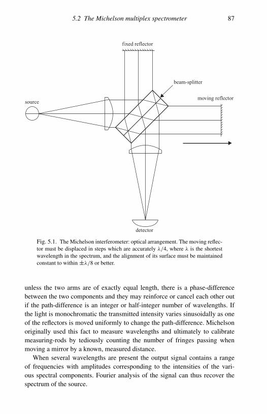
5.2 The Michelson multiplex spectrometer 87
fixed reflector
beam-splitter
moving reflector
detector
source
Fig. 5.1. The Michelson interferometer: optical arrangement. The moving reflec-tor must be displaced in steps which are accurately λ/4, where λ is the shortestwavelength in the spectrum, and the alignment of its surface must be maintainedconstant to within ˙λ/8 or better.
unless the two arms are of exactly equal length, there is a phase-differencebetween the two components and they may reinforce or cancel each other outif the path-difference is an integer or half-integer number of wavelengths. Ifthe light is monochromatic the transmitted intensity varies sinusoidally as oneof the reflectors is moved uniformly to change the path-difference. Michelsonoriginally used this fact to measure wavelengths and ultimately to calibratemeasuring-rods by tediously counting the number of fringes passing whenmoving a mirror by a known, measured distance.
When several wavelengths are present the output signal contains a rangeof frequencies with amplitudes corresponding to the intensities of the vari-ous spectral components. Fourier analysis of the signal can thus recover thespectrum of the source.
88 Applications 3
It was Lord Rayleigh who, in a letter2 to Michelson, pointed out that theintensity of the light in the fringe system is the Fourier transform of the spectrumof the transmitted light, although there were no means at the time of measuringthe intensity, let alone computing its Fourier transform.
With improvements in technology in the latter half of the twentieth cen-tury both light intensity and reflector positions became measurable with thenecessary accuracy. Fourier transforms became computable via the FFT,3 andhigh-resolution Fourier spectrometry became possible. The reasons for doingspectroscopy in this way were two-fold.
(1) The ‘throughput’ or ‘light-grasp’ of an interferometer is greater by a fac-tor of several hundred than that of a grating spectrometer of the sameaperture.
(2) There is a substantial gain in signal-to-noise ratio in infra-red spectroscopy,where electronic noise in the detector is the chief source of noise, since thewhole spectrum is being observed at once instead of having small wave-length intervals selected and measured sequentially by a monochromator.This gain is generally known as the multiplex advantage or the Fellgettadvantage after its discoverer.4
All this allows the analysis of very faint astrophysical or aeronomic sources,or the very rapid measurement of infra-red absorption spectra, sometimesin ‘real-time’ as gaseous fractions come successively through from a gas-chromatograph column to an absorption cell.
There were formidable technical problems to be overcome, since the deviceis mechanically equivalent to a grating-ruling engine with a new grating ruledevery time a spectrum is measured, and a similar precision is needed.
5.2.1 The theory of the Michelson–Fourier spectrometer
In normal adjustment, the focusing lens produces a series of concentric fringesat its focal plane, and there is an aperture through which light from one fringecan pass through to the detector. This aperture is equivalent to the slit of agrating spectrometer. Light of wavenumber ν arriving at the beam splitter canbe described5 by
A D A0e2πiνt
2 Lord Rayleigh, Phil. Mag. 34 (1892), 407. 3 See Chapter 9.4 P. B. Fellgett, Proc. Phys. Soc. B 62 (1949), 529.5 It is more convenient to consider wavenumber rather than wavelength in this type of
spectroscopy.

5.2 The Michelson multiplex spectrometer 89
and immediately after the beam-splitter the two emerging wavefronts, ignoringabsorption, are
A1 D A2 DA0p
2e2πiνt .
If the two beams travel distances d1 and d2 in the two arms of the interfer-ometer, then on recombining they emerge in the transmitted direction as
Atrans D
[A(0)
2e2πiνd1 C
A0
2e2πiνd2
]e2πiνt .
Notice, incidentally, that even if the transmitted and reflected amplitudes arenot equal, each beam experiences one transmission and one reflection and thetwo finally transmitted amplitudes are (or ought to be) the same.
The transmitted intensity, which is what the detector sees, is then
I DjA0j
2
2[1C cos(2πν(d1 � d2))]
and from here on we shall refer to (d1 � d2) as the path-difference .So much for monochromatic light. In reality a monochromatic beam would
convey no power, since power is proportional to bandwidth, and the intensityreceived by the detector from a source of infinitesimal bandwidth, dν, can bedescribed by
I (ν)dν DI0(ν)dν
2[1C cos(2πν)],
again neglecting losses in the beam-splitter, scattering and other practicalmatters.
Now, if a real source of light of spectral power density S(ν) is sent throughthe instrument the power received at the detector is
I () D∫ 1
0
S(ν)dν
2[1C cos(2πν)]
DS
2C
1
2
∫ 1
0S(ν)dν cos(2πν)
and we generally write this expression as
2I () � S D J () D∫ 1
0S(ν)dν cos(2πν),
where S represents the total power delivered to the detector. J (), by itsdefinition, may well be negative when the path-difference is such as to sendhalf the incident power back to the source.

90 Applications 3
More succinctly, we write
J ()• S(ν).
The ‘interferogram’, J (), which is what is recorded, is the Fourier cosinetransform of S(ν), the spectral power density.
Various practical matters intervene. Before the days of the digital computerand even then only after the discovery or invention of the fast Fourier transform(q.v.), there was no real possibility of doing serious Fourier spectroscopy despitethe display of much ingenuity in the invention of analogue devices for carryingout the transform. In modern practice the interferogram is recorded digitally,either as the path-difference is changed continuously by a smooth motionof one of the reflectors, or by a step-by-step change of path-difference, a‘sample’ being taken at each step. Here the sampling theorem intervenes and,in principle, the interferogram should be sampled at intervals of path-differencenot greater than the reciprocal of twice the highest wavenumber in the spectrum.In practice this may be wasteful if the source occupies less than an octave of theelectromagnetic spectrum and an analysis of the complete interferogram wouldonly show that large parts of the spectrum are empty. With suitable opticalfiltering, step-lengths can be made larger and the spectrum recovered from ahigher alias of the true spectrum.
Again, in practice, optical and mechanical shortcomings make it difficultto find the exact position of zero path-difference and there may be wave-length dispersion in the optics, so that the position of zero path-difference iswavenumber-dependent. Various techniques are in use to correct for theseinstrumental defects, for example by using the interpolation theorem to find the‘true’ sample magnitudes (what they would have been if the samples had beentaken exactly from zero path-difference) and by computing the power transform.
The similarity to the mechanism of a grating-ruling engine extends to similarerrors of measurement. If, for example, there is a cyclic variation in the steplength, there will be spurious satellite lines.
The technique generally is valuable only where detector noise predominates.In the visible and ultra-violet, photo-electric detectors are chiefly used andphoto-electron shot noise from the incoming signal is the chief noise source.Then not only is there no multiplex advantage, but there is actually a multiplexdisadvantage, since photo-electron shot noise from a dominant emission lineappears throughout the recovered spectrum and can swamp all the other faintemission lines which may be present.
Other Fourier-transform-related processes are involved in the analysis of theinterferogram. If, for example, the path-difference has been changed smoothlyinstead of step-wise, each sample recorded for the interferogram is accumulated
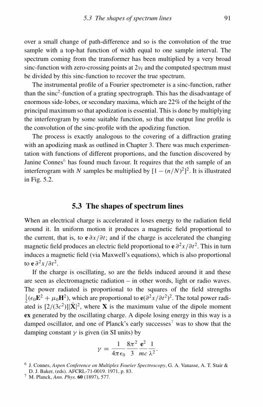
5.3 The shapes of spectrum lines 91
over a small change of path-difference and so is the convolution of the truesample with a top-hat function of width equal to one sample interval. Thespectrum coming from the transformer has been multiplied by a very broadsinc-function with zero-crossing points at 2νf and the computed spectrum mustbe divided by this sinc-function to recover the true spectrum.
The instrumental profile of a Fourier spectrometer is a sinc-function, ratherthan the sinc2-function of a grating spectrograph. This has the disadvantage ofenormous side-lobes, or secondary maxima, which are 22% of the height of theprincipal maximum so that apodization is essential. This is done by multiplyingthe interferogram by some suitable function, so that the output line profile isthe convolution of the sinc-profile with the apodizing function.
The process is exactly analogous to the covering of a diffraction gratingwith an apodizing mask as outlined in Chapter 3. There was much experimen-tation with functions of different proportions, and the function discovered byJanine Connes6 has found much favour. It requires that the nth sample of aninterferogram with N samples be multiplied by [1 � (n/N )2]2. It is illustratedin Fig. 5.2.
5.3 The shapes of spectrum lines
When an electrical charge is accelerated it loses energy to the radiation fieldaround it. In uniform motion it produces a magnetic field proportional tothe current, that is, to e ∂x/∂t ; and if the charge is accelerated the changingmagnetic field produces an electric field proportional to e ∂2x/∂t2. This in turninduces a magnetic field (via Maxwell’s equations), which is also proportionalto e ∂2x/∂t2.
If the charge is oscillating, so are the fields induced around it and theseare seen as electromagnetic radiation – in other words, light or radio waves.The power radiated is proportional to the squares of the field strengths12 (ε0E2 C µ0H2), which are proportional to e(∂2x/∂t2)2. The total power radi-ated is [2/(3c2)]jXXj2, where X is the maximum value of the dipole momentex generated by the oscillating charge. A dipole losing energy in this way is adamped oscillator, and one of Planck’s early successes7 was to show that thedamping constant γ is given (in SI units) by
γ D1
4πε0
8π2
3
e2
mc
1
λ2.
6 J. Connes, Aspen Conference on Multiplex Fourier Spectroscopy, G. A. Vanasse, A. T. Stair &D. J. Baker, (eds). AFCRL-71-0019. 1971, p. 83.
7 M. Planck, Ann. Phys. 60 (1897), 577.

92 Applications 3
Fig. 5.2. The Connes apodizing function for infra-red Fourier spectroscopy andits effect on the instrumental profile. Without it each emission line in the spectrumwould be represented by a sinc-function with secondary maxima �22% of theprincipal maximum in height.
The equation of motion for an oscillating dipole is then the usual dampedharmonic oscillator equation:
x C γ x C Cx D 0,
where C is the ‘elastic’ coefficient, which depends on the particular dipole, andwhich describes its stiffness and the frequency of the oscillation. Here γ is ofcourse the damping coefficient which determines the rate of loss of energy.

5.3 The shapes of spectrum lines 93
The solution of the equation is well known, being
f (t) D e�γ
2 t(Ae2πiν0t C Be�2πiν0t
),
and it is convenient to put A D 0 here so that the amplitude, as a function oftime, is
f (t) D e�γ
2 tBe�2πiν0t .
The Fourier transform of this gives the spectral distribution of amplitude and,when multiplied by its complex conjugate, gives the spectral power density:
φ(ν) D∫ 1
0e�
γ
2 tBe2πiν0t e�2πiνt dt
(the lower limit of integration is 0 because the oscillation is deemed to beginthen). On integrating we get
φ(ν) D e�γ
2 t
[e2πi(ν0�ν)t
2πi(ν0 � ν) � γ /2
]1
0
D1
2πi(ν0 � ν) � γ /2.
The spectral power density is then
I (ν) D1
4π2(ν0 � ν)2 C (γ /2)2
and the line profile is the Lorentz profile discussed in Chapter 1. See Fig. 5.3.The same equation can be derived quantum mechanically8 for the radiation
of an excited atom. The constant γ /2 is now the ‘transition probability’, thereciprocal of the ‘lifetime of the excited state’ if only one downward transitionis possible. The FWHM of a spectrum line emitted by an ‘allowed’ or ‘dipole’atomic transition of this sort is usually called the ‘natural’ width of the line. Theshape occurs yet again in nuclear physics, this time called the ‘Breit–Wignerformula’, and describing in the same way the energy spread in radioactive-decay energy spectra. The underlying physics is obviously the same as in theother cases.
There is thus a direct link between the transition probability and the breadthof a spectrum line, and in principle it is possible to measure transition probabil-ities by measuring this breadth. With typical ‘allowed’ or ‘dipole’ transitions –the sort usually seen in spectral discharge lamps – the transition probabilitiesare in the region of 108 s�1 and the breadth of a spectrum line at 5000 A – in thegreen – is about 0.003 A. This requires high resolution, a Fabry–Perot etalonfor instance, to resolve it. The measurement is quite difficult since atoms in a
8 See, for example, N. F. Mott & I. N. Sneddon, Wave Mechanics and its Applications, OxfordUniversity Press, Oxford, 1948, Chapter 10, Section 48.

94 Applications 3
Fig. 5.3. The amplitude of a damped harmonic oscillator and the correspondingspectrum line profile: a Lorentz function with FWHM γ /(2π ). This would be theshape of a spectrum line emitted by an atomic transition if the atoms were heldperfectly still during their emission.
gas are in violent motion, and a collimated beam of excited atoms is requiredin order to see the natural decay by this means.
The violent motion of atoms or molecules in a gas is described by theMaxwellian distribution of velocities. The kinetic energy has a Boltzmanndistribution, and the fraction of atoms with velocity v in the observer’s line-of-sight has a Gaussian distribution:
n(v) D n0e�mv2/(2kT )

5.3 The shapes of spectrum lines 95
with a proportionate Doppler shift, giving a Gaussian profile to what otherwisewould be a monochromatic line:
I (λ) D I0e�(λ�λ0)2/a2
.
The width parameter, a, comes from the Maxwell velocity distribution anda2 D 2λ2
0kT /(mc2), where k is Boltzmann’s constant, T the temperature, m
the mass of the emitting species and c the speed of light.When we substitute numbers into this formula we find that the inten-
sity profile is a Gaussian with FWHM proportional to wavelength, and withλ/λ D 7.16 � 10�7pT/M , where M is the molecular weight of the emittingspecies.
This Doppler broadening, or temperature broadening, by itself would give adifferent line shape from that caused by radiation damping: a Gaussian profilerather than a Lorentz profile. Unless the emitter has a fairly high molecularweight or the temperature is low, the Doppler width is much greater than thenatural width. However, the line shape that is really observed, after makingallowance for the instrumental function, is the convolution of the two into whatis called a ‘Voigt’ profile,
V (λ) D G(λ) � L(λ).
The Fourier transform will be the product of another Gaussian shape andthe Fourier transform of the Lorentz shape. This Lorentz shape is a spectralpower density and its Fourier transform is, according to the Wiener–Khinchinetheorem, the autocorrelation of the truncated exponential function representingthe decay of the damped oscillator. This autocorrelation is easily calculated.Let s be the variable paired with λ. Then L(λ)• l(s), where
l(s) D∫ 1
s
e�γ
2 s0
e�γ
2 (s0�s) ds0
D
1
γe�
γ
2 s γ > 0,
1
γe
γ
2 s γ < 0.
Autocorrelations are necessarily symmetrical and so we can write
l(s) D2
γe
γ
2 jsj.
For positive values of s, the Fourier transform of the Voigt line profile is theproduct
v(s) D e�π2s2a2e�
γ
2 s

96 Applications 3
and a graph of loge v(s) versus s is a parabola. From this parabola the two quan-tities γ and a can be extracted by elementary methods, and the two componentsof the convolution are separated.
Voigt profiles occur fairly frequently in spectroscopy. Not only is the lineprofile of a damped oscillator a Lorentz curve, but the instrumental profile of aFabry–Perot etalon is the convolution of a Lorentz profile9 with a Dirac comb.Fabry–Perot fringes, when used to measure the temperature of a gas or a plasma,therefore show Voigt profiles and if the instrument is used properly – that iswith the appropriate spacing between the plates for the given experiment – theLorentz half-width will be similar to the Gaussian half-width.
Other causes of spectral line shapes can easily be imagined. If the pressureis high, atoms will collide with each other before they have had time to finishtheir transition. The decaying exponential is then cut short, and the resultingline shape is the convolution of the Lorentz profile with a sinc-function. Thewidth of the sinc-function will be different for every decay, with a Poissondistribution about some average value. The resulting spectrum line then shows‘pressure-broadening’, which increases as the intercollision time diminishes,i.e. as the pressure increases. This is a phenomenon which can be used, forexample, to diagnose conditions in remote plasmas.
9 Because where the transmitted intensity is non-trivial the sine of the phase-angle in the Airyformula can be replaced by the angle itself.

6
6.1 Cartesian coordinates
The extension of the basic ideas to two dimensions is simple and direct. Asbefore, we assume that the function F (x, y) obeys the Dirichlet conditions andwe can write
A(p, q) D∫ 1
yD�1
∫ 1
xD�1
F (x, y)e2πi(pxCqy) dx dy,
F (x, y) D∫ 1
qD�1
∫ 1
pD�1
A(p, q)e�2πi(pxCqy) dp dq.
The space of the transformed function is of course two-dimensional, like theoriginal space. The extension to three or more dimensions is obvious.
It sometimes happens that the function F (x, y) is separable into a productf1(x)f2(y). In this case the Fourier pair, A(p, q), is separable into φ1(p)φ2(q)and we find separately that
f1(x)• φ1(p); f2(y)• φ2(q).
If F (x, y) is not separable in this way then the transform must be done intwo stages:
A(p, q) D∫ 1
�1
e2πiqy
{∫ 1
�1
F (x, y)e2πipx dx
}dy,
and whether the x-integral or the y-integral is done first may depend on theparticular function, F .
97
Two-dimensional Fourier transforms

98 Two-dimensional Fourier transforms
6.2 Polar coordinates
Sometimes – often – there is circular symmetry and polar coordinates can beused. The transform space is also defined by polar coordinates, ρ and φ, andthe substitutions are
x D r cos θ ; y D r sin θ ;
p D ρ cos φ; q D ρ sin φ.
Then
A(ρ, φ) D∫ 1
rD0
∫ 2π
θD0F (r, θ )e2πi(ρ cos φ � r cos θ C ρ sin φ � r sin θ)r dr dθ,
where r dr dθ is now the element of area in the integration, as can be seendirectly or from the Jacobian ∂(x, y)/∂(r, θ ).
This shortens to
A(ρ, φ) D∫ 1
rD0
∫ 2π
θD0F (r, θ )e2πiρr cos(θ�φ)r dr dθ
and, if the function F is separable into P (r)�(θ ), the integrals separate into∫ 1
rD0P (r)
{∫ 2π
θD0�(θ )e2πiρr cos(θ�φ) dθ
}r dr.
If there is circular symmetry A is a function of r only, and �(θ ) D 1. We canwrite
A(ρ, φ) D∫ 1
rD0P (r)
[∫ 2π
θD0e2πiρr cos(θ�φ) dθ
]r dr.
We now put θ � φ D α, a new independent variable, with dα D dφ (the inte-gral, being taken around 2π , does not depend on the value of θ ).
Then the θ -integral becomes∫ 2π
0e2πiρr cos α dα
and this (see Appendix A.2) is equal to 2πJ0(2πρr), where J0 denotes thezeroth-order Bessel function.
Then
A(ρ) D 2π
∫ 1
0P (r)rJ0(2πρr)dr,
which is known as a Hankel transform. It is a close relative of the Fouriertransform.

6.3 Theorems 99
The Bessel functions of any order n, Jn(x), have the property that whenthey are multiplied by x1/2 they form an orthogonal set1 like the trigonometricfunctions: ∫ 1
0xJn(x)Jm(x)dx D δn
m,
where δnm is the usual Kronecker-delta (δn
m D 0 if m 6D n and δmm D 1).
Consequently there is an inversion formula as in the Fourier transform, sothat P (r) can be recovered from
P (r) D 2π
∫ 1
0A(ρ)ρJ0(2πρr)dρ
and the two functions are symbolically linked by
P (r), A(ρ).
6.3 Theorems
Some, but not all, of the theorems derived in Chapter 2 carry over intotwo dimensions. As above, assume that P (r), A(ρ); then we have thefollowing.
� The similarity theorem: P (kr), (1/k2)A(ρ/k).� The addition theorem: P1(r)C P2(r), A1(ρ)C A2(ρ).� Rayleigh’s theorem:∫ 1
0jP (r)j2r dr D
∫ 1
0j�(ρ)j2ρ dρ.
� The convolution theorem. There is a convolution theorem like that in onedimension but one of the functions has to explore the whole plane in twodimensions instead of just sliding over the other. The product integral is doneat each point in the plane to obtain the convolution:
C(r 0) D P1(r) � �P2(r) D∫ 1
rD0
∫ 2π
θD0P1(r)P2(R)r dr dθ,
where R2 D r2 C r 02 � 2rr 0 cos θ and the symbol �� is used to denote atwo-dimensional convolution. Then
C(r), A1(ρ)A2(ρ).
1 A proof of the orthogonality is given by Bracewell (see the bibliography).

100 Two-dimensional Fourier transforms
6.4 Examples of two-dimensional Fourier transforms withcircular symmetry
� The top-hat function, also known as ‘circ’ or ‘disk’:
P (r) D
{h, 0 < r < a,
0, a < r <1,
A(ρ) D 2πh
∫ a
0r � J0(2πρr)dr.
We use the property (see Appendix A.2)
d
dx(xJ1(x)) D xJ0(x).
Let
2πρr D x; 2πρ dr D dx.
Then
A(ρ) D 2πh
∫ 2πaρ
0
x
2πρJ0(x)
dx
2πρ
Dh
2πρ2
∫ 2πaρ
0xJ0(x)dx D
h
2πρ2[xJ1(x)]2πaρ
0
Dah
ρJ1(2πaρ) D πa2h
{2J1(2πaρ)
2πaρ
}
and finally
A(ρ) D πa2h Jinc(2πaρ), where Jinc(x) D2J1(x)
x.
Jinc contains the factor of 2 in order that Jinc(0) D 1.This, with a as the aperture radius and ρ as sin θ/λ, gives the amplitude
of diffraction of light or radio waves at a circular aperture. The intensitydistribution, which is the square modulus of this, is the famous ‘Airy disc’familiar to students of the telescope and other optical imaging instruments.
� The thin annulus. P (r) is a circle of radius a. In optics, for a very thin ringtransmitting light,
P (r) D hδ(r � a).
Then
A(ρ) D 2πh
∫ 1
0rδ(r � a)J0(2πρr)dr
D 2πahJ0(2πaρ).

6.5 Applications 101
6.5 Applications
6.5.1 Fraunhofer diffraction by a rectangular slot
The simple two-dimensional Fraunhofer theory of Chapter 3 can now be elab-orated. There, we assumed that the element dS on the surface S was equal inarea to dx, the width of a slit � unit length perpendicular to the diagram.
Now we can use dS D dx dy, a small rectangle in the diffracting aperture,perpendicular to the direction of propagation, and we can calculate the diffractedamplitude in a direction specified by direction cosines l, m, n. From this wecan calculate the intensity at a point on a plane at a distance z from the aperture.If the amplitude at the element of area dx dy at Q(x, y) is K dx dy, then at P ,on the distant screen, it will be K dx dy e
2πiλ
R0
and, from elementary coordinategeometry, R0 D R � lx �my, where l and m are the direction cosines of theline OP and R is the distance from the origin to the point P on the distantscreen. See Fig. 6.1.
The total disturbance at P is then the sum of all the elementary disturbancesfrom the z D 0 plane, so that we can write
A(p, q) D∫ ∫
apertureK dx dy e
2πi
(Rλ
� lxλ
�my
λ
)
D C
∫ ∫aperture
e�2πi(pxCqy) dx dy,
Fig. 6.1. The two-dimensional diffracting aperture, in Cartesian coordinates.

102 Two-dimensional Fourier transforms
where p D l/λ, q D m/λ and C is a constant which depends on the area of theaperture, and contains the constant phase factors and any other things whichdo not affect the relative intensity in the diffraction pattern.
If the aperture is a rectangle of sides 2a and 2b, the integrals separate:
A(p, q) D C
∫ a
�a
e�2πipx dx
∫ b
�b
e�2πiqy dy,
and the intensity diffracted in the direction whose direction cosines are pλ andqλ is the square-modulus of this:
I (p, q) D I0 sinc2(2πap)sinc2(2πbq).
Notice that, perhaps surprisingly, the intensity at the central peak is proportionalto the square of the area of the aperture.
6.5.2 Fraunhofer diffraction by a circular aperture
If the aperture is circular and of radius a, the Hankel transform is used, withx D r cos θ, y D r sin θ as before and with p D l/λ D ρ cos φ, q D m/λ D
ρ sin φ and ρ2 D p2 C q2.The third direction cosine, n, is given by
n2 D 1 � l2 �m2 D 1 � (pλ)2 � (qλ)2
so that
ρ2 D1
λ2(l2 Cm2) D
1 � n2
λ2
or ρ D sin θ/λ, where θ is the angle between OP and the z-axis.Then, immediately, we have
A(θ ) D A(0)J1(2πa sin θ/λ)
2πa sin θ/λ
and
I (θ ) D I (0)
[J1(2πa sin θ/λ)
2πa sin θ/λ
]2
,
which is the formal equation for the intensity in the Airy disc. Again notice thatI (0) is proportional to the square of the area of the aperture. The total powerin the pattern is of course proportional to the area of the aperture, but as theradius of the diffracting aperture doubles, for example, the pattern on a distantscreen has half the radius and one-quarter the area, out to the first zero-intensityring.

6.6 Solutions without circular symmetry 103
As an exercise, the calculation of the intensity distribution in the diffractionpattern made by an annular aperture can be done. If the inner and outer radii ofthe annulus are a and b, the amplitude function is
A(θ ) D K
[a2 J1(2πa sin θ/λ)
2πa sin θ/λ� b2 J1(2πb sin θ/λ)
2πb sin θ/λ
]
and the intensity distribution is the square of this.A graph of this function shows that the central maximum is narrower than
that of the Airy disc for the same outer radius. A telescope with an annularaperture apparently beats the ‘Rayleigh criterion’ for spatial resolution. How-ever, it does so at the expense of putting a lot of intensity into the ring aroundthe central maximum, and the gain is usually more illusory than real.
6.6 Solutions without circular symmetry
In general, provided that the aperture function can be separated into P (r) and�(θ ), then, as we saw earlier,
A(ρ, φ) D∫ 1
rD0P (r)
{∫ 2π
θD0�(θ )e2πiρr cos(θ�φ) dθ
}r dr.
Consider the interference pattern of a set of apertures – or antennae – equallyspaced around the circumference of a circle. If there are N of them, the θ -dependent function is
�(θ ) DN�1∑
0
δ(θ � 2πn/N )
and the r-dependent part is
P (r) D δ(r � a).
In other words, the sources are equally spaced at angles 2π/N around the circleof radius a
Then
A(ρ, φ) D∫ 1
0rδ(r � a)
N�1∑0
e2πiρr cos(2πn/N�φ) dr
D a
N�1∑0
e2πiρa cos(2πn/N�φ).
This is as far as the analysis can be taken. The pattern, I (ρ, φ), can be computedwithout difficulty from this expression, and is a typical example of a problem

104 Two-dimensional Fourier transforms
Fig. 6.2. The cones of maximum intensity in a two-beam interference pattern.The two interfering sources are on the x-axis, above and below the origin.
solved by computer after analysis fails. The particular case of N D 2 yields thefamiliar pattern of two-beam interference, including the hyperbolic shapes ofthe fringes on a distant plane surface:
A(ρ, φ) D a[e2πiaρ cos φ C e2πiaρ cos(π�φ)]
D 2a cos(2πaρ cos φ),
and the intensity pattern is given by
I (ρ, φ) D 4a2 cos2(2πaρ cos φ),
which has maxima when 2aρ cos φ is integer. Since ρ D sin α/λ, the maximaoccur when φ D nλ/2a sin α. Here α is the angle between the z-axis andthe direction of diffraction, and φ is the azimuth (angle in the p, q-plane),so that interference fringes, the maxima of I (ρ, φ), emerge along directionsdefined by the condition (2a/λ)sin α cos φ D constant, that is to say, on conesof semi-angle φ about the φ D 0-axis (see Fig. 6.2). If they are received ona plane perpendicular to the z-axis they show hyperbolic shapes, but on aplane perpendicular to the x-axis (the φ D 0-axis: the axis containing the twosources) the shapes would be concentric circles.
Other cases, such as N D 4, yield to analysis as well. But in general, toparody Clausewitz, it is best to regard computation as the continuation ofanalysis by other means.

7
The physical world seems to comprise four dimensions of space and time,and other dimensions, such as electrical potential or temperature, are usedoccasionally for drawing graphs. For this reason Fourier transforms in three ormore dimensions can be useful sometimes. The extension is not difficult andcan sometimes give greater insight into what is happening in Nature than canmere geometry. This chapter describes some of the functions and ideas whichare helpful in manipulating multi-dimensional Fourier transforms.
7.1 The Dirac wall
This is described by
f (x, y) D δ(x � a)
and is zero everywhere except on the line x D a, where it is infinite. Despitethis infinity, it may be envisaged as a wall, parallel to the y-axis, of unit height,as in Fig. 7.1.
Its two-dimensional Fourier transform (Fig. 7.2) is given by
φ(p, q) D∫ 1
xD�1
∫ 1
yD�1
δ(x � a)e2πipxe2πiqy dx dy
D
∫ 1
yD�1
e2πipae2πiqy dy
D e2πipaδ(q),
which has a complex amplitude1 and is zero except on the line q D 0.
1 In the sense mentioned in Chapter 1, namely that a δ-function is infinite at each point but itsintegral, which we consider to be its ‘amplitude’, is unity.
105
Multi-dimensional Fourier transforms

106 Multi-dimensional Fourier transforms
Fig. 7.1. A simple Dirac wall, f (x, y) D δ(x � a).
Fig. 7.2. The Fourier tranform of a pair of Dirac walls.

7.1 The Dirac wall 107
A pair of these Dirac walls, equally disposed about the y-axis, has a Fouriertransform given by
φ(p, q) D 2δ(q)cos(2πpa).
A wall standing on a line inclined to the y-axis at an angle θ is described byf (x, y) D δ(lx Cmy � c), where l D cos θ , m D sin θ and c is the length ofthe perpendicular from the origin to the line. The δ-function is zero everywhereon the x, y-plane except on the line and its two-dimensional Fourier transformis
φ(p, q) D∫ 1
xD�1
∫ 1
yD�1
δ(lx Cmy � c)e2πipxe2πiqy dx dy.
Do the y-integration first,2
φ(p, q) D1
m
∫ 1
xD�1
e2πipxe2πiq(c�lx)/m dx,
and notice that ‘integration’ here is a simple replacement of the variable in theexponential by the argument of the δ-function.
Then, rearranging the exponents,
φ(p, q) D1
me2πiqc/m
∫ 1
xD�1
e2πix(p�lq/m) dx
D e2πiqc/mδ(mp � lq),
which is zero except on the line mp � lq D 0 in the p, q-plane.Equally, the y-integration could have been done first, in which case the
Fourier transform would have been
e2πipc/lδ(mp � lq).
The period in the phase-factor is 1/c and it is measured along the direc-tion of the line mp � lq D 0 in p, q-space. As we shall see later, it is possi-ble to envisage a one-dimensional variable u D p/l or q/m, conjugate to c,along that line, and then the above function describes a complex sinusoid ofperiod 1/c along the Dirac wall. Its one-dimensional Fourier transform alongthat line would then be a δ-function at a distance c from the origin, situ-ated at the point lc,mc in x, y-space. This δ-function would lie on the linemx � ly D 0.
This is the place to mention that much insight can be gained by superposingthe two planes so that the p- and q-axes of one coincide with the x- and y-axes
2 Bearing in mind from Chapter 1 that δ(lx C my � c) D (1/m)δ(y � (c � lx)/m).

108 Multi-dimensional Fourier transforms
of the other. In this example, the Fourier transform of the Dirac wall lies on aline in the p, q-plane perpendicular to the wall in the x, y-plane.
A pair of Dirac walls, equally disposed on either side of the origin, has atwo-dimensional Fourier transform given by
δ(lx Cmy � c)C δ(lx Cmy C c)• δ(mp � lq) � 2 cos(2πqc/m),
that is to say, a Dirac wall with a sinusoidally-varying amplitude and lying onthe line mp � lq D 0.
Notice particularly that, with this superposition of the two planes, the func-tion and its transform are related in spatial position, irrespective of the orienta-tion3 of the coordinate systems chosen. In this example they lie on perpendicularDirac walls.
7.2 Computerized axial tomography
A particularly useful application of these ideas is to be found in computerizedtransverse axial scanning tomography, vulgarly known as CAT-scanning orC-T scanning. Imagine a Dirac wall taking a vertical slice through a two-dimensional function F (x, y) lying on the x, y-plane (Fig. 7.3(a)). If the wallstands on the line lx Cmy � c D 0 the product is zero everywhere except onthe line. On the line stands a Dirac wall (Fig. 7.3(b)) with amplitude varying asF (x, (c � lx)/m). The line-integral (Fig. 7.3(c))
Pl(c) D∫ 1
�1
F (x, y)δ(lx Cmy � c)ds (7.1)
(where ds is the line element along the direction defined by l) depends onlyon l and c. Incidentally, Pl(c) is known as the Radon transform4 of F (x, y). Itcan be imagined, as in the previous section, as a δ-function of amplitude Pl(c)standing on the line mx � ly D 0 at a distance c from the origin. With c asvariable it becomes a function of c along the line and this function is called theprojection of F (x, y) in the direction θ where cos θ D l.
Now, as the direction θ rotates from 0 to π , the various functions Pl(c)sweep out a two-dimensional function Q(x, y) on the x, y-plane.
What is more interesting, however, is the function which results from firsttaking the one-dimensional Fourier transform of Pl(c) along the line mx � ly D
0, with c as variable on the x, y-plane and u as its conjugate on the p, q-plane.
3 But not of the position of the origin.4 Vide e.g. S. R. Deans, The Radon Transform and Some of its Applications, John Wiley, New
York, 1983.

7.2 Computerized axial tomography 109
θ
φ1(u)
q
p
q
p
u
um
ul
ΦΦ(ul,um)
F(x,y)
y
x
x
θ
θ
θ
θ
θ
lx + my + c = 0
lx + my + c = 0
F(x,y) δ(lx + my + c)
F(x,y) δ(lx + my + c) dxdyh =
P1(c)
c
x
y
θ
p
hq1/c
y
θ
(a) (e)
(f)
(b)
(c)
(d)
Fig. 7.3. The steps in computerized axial tomography. (a) A Dirac wall through thefunction F (x, y). (b) The slice to be integrated along the line lx C my C c D 0.
(c) The integral of the slice along the line, making one point of the function P (c),the Radon transform of F (x, y). (d) The one-dimensional Fourier transform of thatpoint with c as variable, lying on the line in conjugate p, q-space perpendicularto the Dirac wall. (e) The complete one-dimensional Fourier transform, φ(u), ofP (c) in p, q-space. (f) The point on this function which defines one point of thetwo-dimensional function �(ul, um) which is shown to be the two-dimensionalFourier transform of the original F (x, y).
In the p, q-plane this Fourier transform, φl(u), will lie on the line mp � lq D 0which is superimposed on mx � ly D 0 on the x, y-plane. This set of Fouriertransforms, too, sweeps out a two-dimensional function �(p, q) (the func-tion φl(u) in Fig. 7.3(e)) as the direction of the projection changes from0 to π .
We now demonstrate the remarkable fact that �(p, q) is the two-dimensionalFourier transform of F (x, y).

110 Multi-dimensional Fourier transforms
To do this we first of all write δ(lx Cmy � c) as a one-dimensional Fourierintegral, using c as the variable and u as its conjugate:
δ(lx Cmy � c) D∫ 1
uD�1
e2πi(lxCmy�c)u du
D
∫ 1
uD�1
e2πiu(lxCmy)e�2πicu du,
and if we insert this into the equation for Pl(c) (equation (7.1)) we find
Pl(c) D∫ 1
xD�1
∫ 1
yD�1
F (x, y)∫ 1
uD�1
e2πiu(lxCmy)e�2πicu du dx dy
and, on changing the order of integration,
Pl(c) D∫ 1
uD�1
(∫ 1
xD�1
∫ 1
yD�1
F (x, y)e2πiu(lxCmy) dx dy
)e�2πicu du.
Within the brackets is �(ul, um), the two-dimensional Fourier transform ofF (x, y), and notice (Fig. 7.3(e)) that on the p, q-plane ul D p and um D q.
Thus
Pl(c) D∫ 1
�1
�(ul, um)e�2πicu du,
whence, for a fixed direction θ ,
�(ul, um) D �(p, q) D∫ 1
�1
Pl(c)e2πicu dc.
This is still a one-dimensional transform and it defines �(p, q) along theline mp � lq D 0. In Radon transform theory it is called the projection slicetheorem.
Thus, if we know Pl(c) for all azimuths θ , from 0 to π , and do the completeset of one-dimensional transforms, the two-dimensional function �(p, q) isknown. The original function F (x, y) is then obtained from
F (x, y) D∫ 1
�1
∫ 1
�1
�(p, q)e�2πi(pxCqy) dp dq.
If a three-dimensional object is partially transparent to radiation such as X-rays, visible light or a particle beam, it is possible to make a two-dimensionalmap of the absorption coefficient (α) on a plane section through it. Whenmonochromatic radiation is transmitted through the object it is attenuated

7.2 Computerized axial tomography 111
according to Beer’s law, which states that the intensity of the radiation trans-mitted in the x-direction falls according to
∂I
∂xD �Iα,
where I is the intensity at the point x along the direction of transmission, andα is the absorption coefficient for that wavelength or frequency. The coefficientdepends on the nature of the absorbing material and, if the absorption is constantalong the path, Beer’s law in one dimension takes the form
I (x) D I0e�αx.
If α varies from point to point, then the integral along the transmission path(the ‘line-integral’) must be taken and
I (x) D I0e�∫ x
0 α(x) � dx.
From this the following useful equation emerges:∫ x
0α(x) � dx D ln(I0/I (x)).
The function of computer-aided tomography is to make a two-dimensionalplot – the map – of α in a plane slice through the object. Notice that if thesource and the detector are both outside the object then the line-integral of α isidentical with ∫ 1
�1
α(x) � dx D ln(I0/I (x)).
Consider an absorbing object – a skull, for example – through which anarrow beam of X-rays can be transmitted from a source to a detector. Theline-integral of the absorption coefficient α follows from the logarithm of theratio of the intensity at the source to the intensity at the detector.
We now use this narrow beam as a saw-blade to ‘cut’ a plane section throughthe object.
In Fig. 7.3 the z-axis is used to depict the absorption coefficient, α(x, y), inthe section and the radiation beam is directed along the line lx Cmy � c D 0.We replace the F (x, y) by α(x, y) in equation (7.1):
Pl(c) D∫ 1
�1
α(x, y) � δ(lx Cmy � c)ds.
As the source and detector move together in the x, y-plane in a directionperpendicular to the transmission direction, c is changing while l is constant.

112 Multi-dimensional Fourier transforms
The beam, as it moves, takes a slice through the absorbing object (hence theword ‘tomography’) and there will be a measurement of the line-integral Pl(c)as a function of c (Fig. 7.3(c)).
The one-dimensional Fourier transform, φl(u), of Pl(c) maps out, as thedirection θ of the projection changes, the two-dimensional function �(p, q),the aggregate of these φ-functions over all azimuths and this, as we have seen,is the two-dimensional Fourier transform of α(x, y).
This is the central idea in computerized axial tomography.
The inevitable conclusion is that, provided that Pl(c) is measured for everyazimuth θ (θ D cos�1l) from θ D 0 to θ D 180ı, and the one-dimensionalFourier transforms are taken, then the function �(ul, um) is known over thewhole p, q-plane5 and the inverse transform of �(ul, um) is α(x, y), the orig-inal desired function:
α(x, y) D∫ 1
�1
∫ 1
�1
�(q, p) � e�2πiqxe�2πipy dq � dp.
The function α(x, y) then represents the two-dimensional distribution ofdensity, or absorption cross-section, of X-rays or other exploring radiationbeams by the material through which the radiation passes.
The practical implementations6 of the idea have been manifold and to theuniversal public good. This brief description ignores the extraordinary exten-sions of the idea7 in areas as diverse as cosmology and geophysics, and it mustalso be mentioned that other methods than Fourier transforms may be used torecover the required data. There can have been few inventions more deservingof a Nobel prize than this one.
7.3 A ‘spike’ or ‘nail’
This is described by a two-dimensional δ-function, δ(x � a)δ(y � b), and iszero everywhere in the x, y-plane except at the point (a, b). Being the productof a function of x and a function of y, it is separable and its Fourier transformis e2πipae2πiqb.
5 Or as much of it as the resolution of the source and detector will permit. Instrumentalconsiderations limit the spatial frequencies accessible to a CAT-scanner and only a limitedarea – about 2 mm�2 – of frequency-space (the p, q-plane) is useable in practice with X-raytomography.
6 The 1979 Nobel prize for physiology and medicine was awarded to G. N. Hounsfield andA. Cormack for the invention of CAT-scanning. The prototype CAT-scanner, constructed byEMI, went into service at the Atkinson Morley Hospital, Wimbledon, in 1971.
7 Described, for example, by Herman (see the bibliography).

7.3 A ‘spike’ or ‘nail’ 113
Fig. 7.4. The Fourier transform of a pair of nails at ˙(x, y).
A pair of such nails equally disposed about the origin is described by
f (x, y) D δ(x � a)δ(y � b)C δ(x C a)δ(y C b)
and its Fourier transform is
φ(p, q) D 2 cos[2π (pa C qb)].
This is a corrugated sheet. Lines of constant phase (wave crests) lie on the linespa C qb D integer, and are illustrated in Fig. 7.4 and again, on superposition,the line joining the nails on the x, y-plane is perpendicular to the wave crestson the p, q-plane.

114 Multi-dimensional Fourier transforms
7.4 The Dirac fence
This is an infinite row of equally-spaced δ-functions (the fence-posts) along aline. When it runs along the x-axis and the spacing of the posts is a, the fenceis described by
f (x, y) D
[1∑
nD�1
δ(x � na)
]δ(y) DШa(x)δ(y).
Its Fourier transform follows from the Fourier transform of a Ш-functionmentioned in Chapter 1 and is (1/a)Ш1/a(p), a parallel set of walls, all parallelto the q-axis, with spacing 1/a.
If the fence is inclined to the x-axis at an angle θ , then l D sin θ andm D cos θ define the direction of the line of the fence, and the fence is describedby
f (x, y) D
[1∑
nD�1
δ(lx Cmy � na)
]δ(mx � ly).
The first factor requires the function to be zero except when lx Cmy D na
(thus defining a set of parallel walls) and the second requires that it be zeroexcept on a line perpendicular to the first set, passing through the origin. Thiscan also be written as
f (x, y) DШa(lx Cmy)δ(mx � ly).
The Fourier transform can be seen graphically as the convolution of the twoseparate transforms. The transform of the first factor is
φ1(p, q) D∫ 1
�1
∫ 1
�1
1∑nD�1
δ(lx Cmy � na)e2πipxe2πiqy dx dy
and once more the simple rule for integrating a product which includes aδ-function applies:
φ1(p, q) D1
l
∫ 1
�1
1∑nD�1
e2πip(na�my)/le2πiqy dy
D1
l
1∑nD�1
e2πipna/l
∫ 1
�1
e2πiy(q�pm/l) dy
D δ(ql � pm)1∑
nD�1
e2πipna/l,

7.5 The ‘bed of nails’ 115
Fig. 7.5. (a) A line of fence-posts of spacing c and (b) its Fourier transform, aseries of parallel walls a distance 1/c apart.
which is a row of fence-posts spaced 1/a apart8 lying on the linelq D mp.
The second factor transforms similarly:
φ2(p, q) D∫ 1
�1
∫ 1
�1
δ(mx � ly)e2πipxe2πiqy dx dy
D1
m
∫ 1
�1
e2πip(ly/m)e2πiqy dy
D δ(lp Cmq),
which is a wall passing through the origin, lying on the line lp D �mq, thatis, perpendicular to the fence-post of the first factor when the p, q-plane issuperimposed on the x, y-plane.
The convolution of these two factors, φ1(p, q) � � φ2(p, q) D w(p, q), isan infinite series of parallel walls, spaced 1/a apart, lying on lines parallelto the line lp D �mq. On superposition of the two spaces, these walls areperpendicular to the original fence line. See Fig. 7.5.
7.5 The ‘bed of nails’
Now consider the convolution of two fences, f1 and f2. Let each lie on aline through the origin, at angles θ1 and θ2 and with spacings a1 and a2. Theconvolution, f1 � � f2, will be a two-dimensional array of δ-functions – a ‘bedof nails’ (Fig. 7.6).
8 Actually the product of a wall lying on the line ql D pm and an infinite set of walls of spacinga/l lying perpendicular to the p-axis.

116 Multi-dimensional Fourier transforms
Fig. 7.6. The convolution of two lines of fence-posts, (a) and (b), to give a ‘bedof nails’, (c).
The Fourier transform of this convolution is the product w1w2 of thetwo transforms, each one a series of parallel walls, and differs from zeroonly when both factors are different from zero. This gives another ‘bed ofnails’.
The interesting thing is that the route to w1w2 from f1 � � f2 is not unique.The two-dimensional array w1w2 could have been composed from two differentfactors, both again parallel sets of walls, but transformed from different fencesf 0
1 and f 02 with different spacings a0
1 and a02 and different angles θ 0
1 and θ 02.
But the convolution of this new pair will necessarily yield the same functionf1 � � f2 as before.
The correspondence between the two beds of nails is this: corresponding toany set of parallel lines that can be drawn through points in one plane thereis a point9 in the other. In Fig. 7.7, parallel lines separated by 1/a in oneplane are matched by a point distance a in the other; another set separatedby 1/b correspond to the point distance b, and so on. The whole thing is thetwo-dimensional analogue of the ‘reciprocal lattice’ idea in crystallography.
There is a familiar illustration: seats in a theatre or cinema are arrangedregularly, often staggered so that people do not sit directly behind someone.Alignments of seat-backs can be seen in different directions, and these corre-spond to the lines that can be drawn through beds of nails.
7.6 Parallel-plane delta-functions
In three dimensions the function δ(lx Cmy C nz) describes a function of unitamplitude which is zero except on the plane lx Cmy C nz D 0.
Its three-dimensional Fourier transform is
φ(p, q, r) D∫ 1
�1
∫ 1
�1
∫ 1
�1
δ(lx Cmy C nz)e2πipxe2πiqye2πirz dx dy dz
9 Actually a pair of points – one on either side of the origin.

7.6 Parallel-plane delta-functions 117
Fig. 7.7. Reciprocal lattices: the correspondence between a bed of nails and itsFourier pair. The pair are not unique: dashed lines show other possible Dirac walls,with different spacings, and the letters u and v show the corresponding directionsof the Dirac fences which are their Fourier transforms. In the diagram on the right,u and v are the reciprocals of u and v: the narrow spacing of the walls implies agreater spacing between the fence-posts.
and, after the x-integration,
φ(p, q, r) D1
l
∫ 1
�1
∫ 1
�1
e2πi(p/l)(�my�nz)e2πiqye2πirz dy dz
D1
l
∫ 1
�1
∫ 1
�1
e2πiy(q�mp/l)e2πiz(r�np/l) dy dz,
which is separable into
1
l
∫ 1
�1
e2πiy(q�mp/l) dy
∫ 1
�1
e2πiz(r�np/l) dz
so that
φ(p, q, r) D lδ(lq �mp)δ(lr � np),
a δ-function which, when the coordinate systems are superimposed, is zeroexcept on the line p/l D q/m D r/n, a line through the origin, perpendicularto the original plane in the x, y, z frame.
The extension is intuitive: a pair of parallel planes equally disposed aboutthe origin and each at a distance a from the origin will have as a Fouriertransform a line along which the amplitude varies sinusoidally with period1/a. An infinite sequence of equally separated parallel planes will transformto a row of equally-spaced points along a line passing through the origin and

118 Multi-dimensional Fourier transforms
perpendicular to the planes. It is the three-dimensional version of a Dirac combbut the function differs from zero at isolated points.
7.7 Point arrays
The ideas are even more apparent when transforms are done in three dimen-sions, when point-arrays are defined by products of three three-dimensionalШ-functions. For example, Шa(l1x Cm1y C n1z) defines a set of paral-lel planes on which the function is not zero. The planes have equationsl1x Cm1y C n1z � λa D 0, where l, m and n are direction cosines, λ is anyinteger and a is the perpendicular distance between two adjacent planes.
Two other sets of parallel planes can be defined similarly by Шb(l2x Cm2y C n2z) and Шc(l3x Cm3y C n3z) and the point array or lattice is definedby the product of these three functions.
The Fourier transform of one of these functions is simple:
φ(p, q, r)D∫ 1
�1
∫ 1
�1
∫ 1
�1
1∑λD�1
δ(lxCmyCnz�λa)e2πi(pxCqyCrz) dx dy dz.
Do the x-integral first:
φ(p, q, r) D1
l
1∑λD�1
∫ 1
�1
∫ 1
�1
e2πip(λa�nz�my)/le2πi(qyCrz) dy dz,
where the λ-sum provides the Ш-function and the integral as before is merelythe substitution of the value into the δ-function argument which makes itnon-zero.
The integral is now separable:
φ(p, q, r) D1
l
1∑λD�1
e2πipaλ/l �
∫ 1
�1
e�2πi
(pn
l�r
)zdz
∫ 1
�1
e�2πi
(pm
l�q
)ydy
D1
l
1∑λD�1
e2πipaλ/l �1
nδ(p
l�
r
n
)�
1
mδ(p
l�
q
m
).
The last two factors, the δ-functions, define two planes. The intersection of theplanes defines a line. The sum over λ defines those points on the line where thelattice points exist in p, q, r-space.10
10 By analogy with all the other entities to which the prefix ‘Dirac’ has been attached, the idea ofa ‘Dirac string’ might be advanced to describe a spatial curve on which a three-dimensionalfunction f (x, y, z) is defined, on the understanding that it is zero everywhere except on that

7.8 Lattices 119
Again, if the p, q, r-space is superimposed on the x, y, z-space, we find thatφ(p, q, r) is a set of equispaced points along a line perpendicular to the setof planes defined by δ(lx Cmy C nz � λa) and that the spacing between thepoints is 1/a.
7.8 Lattices
A complete three-dimensional lattice, described by the product of three planarШ-functions of the type Шa(lx Cmy C nz) has as its Fourier transform thetriple convolution of three lines of equispaced points. This gives a new lattice –the reciprocal lattice11 in p, q, r-space, which is used in crystallography. Pointson this reciprocal lattice define various planes in x, y, z-space, which containtwo-dimensional arrays of lattice points. Lines from the origin to points onthe reciprocal lattice define both the orientation and the separation of thecorresponding planes in x, y, z-space.
This now clears up a fundamental problem in describing crystals. The threeШ-functions used to define the crystal lattice in x, y, z-space are not the onlypossible ones. Other sets of planes can be used – an infinite number of possi-bilities exists. The points in the reciprocal lattice define uniquely such sets ofparallel planes. The lines (‘vectors’) from the origin to these points in p, q, r-space are normal to the lattice-planes in x, y, z-space and the length of eachvector is inversely proportional to the separation of the planes in x, y, z-space.The coordinates of the lattice points in p, q, r-space, when multiplied by a fac-tor to make them integer, are the Miller indices, beloved of crystallographers,of the x, y, z-planes.
curve. For example, f (x, y, z)δ(l1x C m1y C n1z)δ(l2x C m2y C n2z) describes a functionwhich is zero everywhere except on the line x/(n1m2 � n2m1) D y/(l1n2 � l2n1) Dz/(l1n2 � l2n1).
11 Vide e.g. H. M. Rosenberg, The Solid State, 3rd edn, Oxford University Press, Oxford, 1988.

8
The formal complex Fourier transform
In physics we are usually concerned with functions of real variables, whichare often experimental curves, data strings, or shapes and patterns. Generallythe function is asymmetrical about the y-axis and so its Fourier transform isa complex function of a real variable; that is, for any value of p, a complexnumber is defined.
Any function obeying the Dirichlet conditions can be divided into asymmetrical and an antisymmetrical part. In Fig. 8.1, for example, and gener-ally, fs(x) D 1
2 [f (x)C f (�x)] and fa(x) D 12 [f (x) � f (�x)]. The symmet-
rical part is synthesized only from cosines and the antisymmetrical part onlyfrom sines. We write
f (x) D fs(x)C fa(x); fs(x)• φs(p); fa(x)• φa(p),
where φs(p), being made of cosines, is real and symmetrical and φa(p) isimaginary and, being made of sines, is antisymmetrical.
We can also define the following.
(a) The phase transform of f (x), which is the function θ (p), where
tan θ (p) D φa(p)/φs(p).
(b) The power transform:
P (p) D jφ(p)j2 D φa(p)2 C φs(p)2.
(c) The modular transform:
M(p) D jφ(p)j D√
φa(p)2 C φs(p)2.
All these have their practical uses, although none of them has a uniqueinverse.
120

The formal complex Fourier transform 121
Fig. 8.1. Dividing a function into symmetrical and antisymmetrical parts.
A useful corollary of the convolution theorem is that if C(x) D f1(x) � f2(x)and C(x)• �(p) then the power transforms of C, f1 and f2, given by j�j2,jφ1j
2 and jφ2j2, are related by
j�j2 D jφ1j2 � jφ2j
2.
A simple example shows the use of phase transforms. Consider for instancea displaced top-hat function (any function would do, in fact), of width a anddisplaced sideways by a distance b.
The function is
f (x) D �a(x) � δ(x � b).
Its Fourier transform is
φ(p) D a sinc(πap) � e2πibp
D a sinc(πap)[
cos(2πbp)C i sin(2πbp)]
and its phase transform is
θ (p) D tan�1(sin(2πpb)/cos(2πpb))
so that θ (p) D 0 when p D 0 and θ (p) D 2π when p D 1/b.Phase transforms are useful when an experimentally measured function,
which should have been symmetrical, has been displaced by an unknownamount from its axis of symmetry – for example by sampling it in the wrongplaces. A quick calculation of a few points on the phase transform will find thedisplacement and allow any adjustments to be made or the true, symmetricalsamples to be computed by interpolation. It also confirms (or not!) that the

122 The formal complex Fourier transform
Fig. 8.2. A top-hat function displaced by half its own width. (a) The dissectionof the top-hat into symmetrical and antisymmetrical parts.
function really is symmetrical, since only then is its phase transform a straightline.
It is worth including here something which will be useful later when con-sidering computing Fourier transforms. Since it is easy to separate the realand imaginary parts of a complex function of x or p and then to divide theseinto their symmetrical and antisymmetrical parts, it is possible to combine tworeal functions of x into a complex function and then separate the combinedcomplex Fourier transform into its constituent parts. This is a useful techniquewhen computing digital Fourier transforms: one can do two transforms for theprice of one.
Written analytically, let the two functions be f1(x) and f2(x) and separateeach into its symmetrical and antisymmetrical parts:
f1(x) D f1s(x)C f1a(x); f2(x) D f2s(x)C f2a(x).

The formal complex Fourier transform 123
Fig. 8.2. (cont.) (b) The cosine transform. (c) The sine transform.
Let
F (x) D f1(x)C if2(x).
Let
F (x)• �(p).
Then
�(p) D∫ 1
�1
[f1(x)C if2(x)]e2πipx dx.

124 The formal complex Fourier transform
Fig. 8.2. (cont.) (d) The transform in perspective. (e) The Nyquist diagram – theview looking along the ν-axis.
Remember that a symmetrical function has only a cosine transform, etc.,
�(p) D∫
f1s(x)cos(2πpx)dx C i
∫f1a(x)sin(2πpx)dx
C i
∫f2s(x)cos(2πpx)dx �
∫f2a(x)sin(2πpx)dx
D φ1s(p)C iφ1a(p)C iφ2s(p) � φ2a(p),
where the meaning of each suffix is the same as in the f -functions.

The formal complex Fourier transform 125
Then
�(p) D [φ1s(p) � φ2a(p)]C i[φ1a(p)C φ2s(p)].
Both the real part and the imaginary part of �(p) now have symmetrical andantisymmetrical components. When �(p) has been computed, it has a real part,�r(p), and an imaginary part, �i(p).
The symmetrical real part is
1
2[�r(p)C�r(�p)] D φ1s(p)
and the antisymmetrical part is
1
2[�r(p) ��r(�p)] D �φ2a(p).
Similarly,
1
2[�i(p) ��i(�p)] D φ1a(p)
and
1
2[�i(p)C�i(�p)] D φ2s(p)
so that, finally,
f1(x)•1
2[�r(p)C�r(�p)]C
(i
2
)[�i(p) ��i(�p)]
•1
2φ1s(p)C
(i
2
)φ1a(p)
and, similarly,
f2(x)•1
2φ2s(p)C
(i
2
)φ2a(p).
In other words, the Fourier transform of f1(x) is 12 � (the symmetrical part of
the real component of �(p) plus i � the antisymmetrical part of the imaginarycomponent of �(p)), and the Fourier transform of f2(x) is 1
2 � (the symmetricalpart of the imaginary component plus i � the antisymmetrical part of the realcomponent). The computer sorts these out without difficulty!
Notice that all the F ’s, �’s, f ’s and φ’s with suffixes are real quantities. Thisis because a computer deals ultimately in real numbers, although its programmay include complex arithmetic. This level of complication is not commonlymet when discussing analytic Fourier transforms. However, computing algo-rithms compute the complex transform whether you like it or not, and the

126 The formal complex Fourier transform
relations above can be used to do tricks in shortening computing time whenyou know that the data represent only real functions.
Diagrammatically, the process can be represented by
f1s(x) cos ! φ1s(p),
f1a i sin! iφ1a,
if2s cos ! iφ2s,
if2a i sin! �φ2a.
A function is said to be Hermitian if its real part is symmetrical and itsimaginary part is antisymmetrical. So, if f1(x) is symmetrical and f2(x) isantisymmetrical, then φ1a 0 and φ2s 0. Then
�(p) D φ1s(p)C φ2a(p)
and is real. Alternatively, the Fourier transform of a real but asymmetricalfunction is Hermitian:
f1(x)• φ1s(p)C iφ1a(p).
9
Discrete and digital Fourier transforms
9.1 History
Fourier transformation is formally an analytic process which uses integral cal-culus. In experimental physics and engineering, however, the integrand maybe a set of experimental data, and the integration is necessarily done artifi-cially. Since a separate integration is needed to give each point of the trans-formed function, the process would become exceedingly tedious if it wereto be attempted manually, and many ingenious devices have been invented forperforming Fourier transforms mechanically, electrically, acoustically and opti-cally. These are all now part of history since the arrival of the digital computerand more particularly since the discovery – or invention – of the ‘fast Fouriertransform’ algorithm or FFT as it is generally called. Using this algorithm, thedata are put (‘read’) into a file (or ‘array’, depending on the computer jargonin use), the transform is carried out, and the array then contains the points ofthe transformed function. It can be achieved by a software program, or by apurpose-built integrated circuit. It can be done very quickly so that vibration-sensitive instruments with Fourier transformers attached can be used for tuningpianos and motor engines, for aircraft and submarine detection and so on. Itmust not be forgotten that the ear is Nature’s own Fourier transformer,1 and,as used by an expert piano-tuner, for example, is probably the equal of anyelectronic simulator in the 20–20 000-Hz range. The diffraction grating, too, isa passive Fourier transformer device, provided that it is used as a spectrographtaking full advantage of the simultaneity of outputs.
The history of the FFT is complicated and has been researched by Brigham2
and, as with many discoveries and inventions, it arrived before the (com-puter) world was ready for it. Its digital apotheosis came with the publication
1 It detects the power transform, and is not sensitive to phase.2 E. O. Brigham, The Fast Fourier Transform, Prentice-Hall, Englewood Cliffs, NJ, 1974.
127

128 Discrete and digital Fourier transforms
of the ‘Cooley–Tukey’ algorithm3 in 1965. Since then other methods havebeen virtually abandoned except for certain specialized cases and this chap-ter is a description of the principles underlying the FFT and how to use it inpractice.
9.2 The discrete Fourier transform
There is a pair of formulae by which sets of numbers [an] and [Am], each sethaving N elements, can be mutually transformed:
A(m) D1
N
N�1∑0
a(n)e2πinm/N ; a(n) DN�1∑
0
A(m)e�2πinm/N . (9.1)
In appearance and indeed in function, these are very similar to the formulaeof the analytic Fourier transform and are generally known as a ‘discrete Fouriertransform’ (DFT). They can be associated with the true Fourier transform bythe following argument.
Suppose, as usual, that f (x) and φ(p) are a Fourier pair. If f (x) is multipliedby a Ш-function of period a then the Fourier transform becomes
�(p) D∫ 1
�1
f (x)Шa(x)e2πipx dx D (1/a)[φ(p) �Ш1/a(p)].
Now suppose that f (x) is negligibly small for all x outside the limits �a/2!(N � 1/2)a, so that there are N teeth in the Dirac comb, and f (x) extends overa range �Na. We rewrite the integral and use the properties of δ-functions sothat
�(p) D∫ 1
�1
1∑nD�1
f (x)e2πipxδ(x � na)dx
D
1∑nD�1
∫ 1
�1
f (x)e2πipxδ(x � na)dx.
Because there are only N teeth in the comb, the sum is finite and the integralmeans substituting the argument of the δ-function as usual.
�(p) DN�1∑nD0
f (na)e2πipna
D (1/a)[φ(p) �Ш1/a(p)].
3 J. W. Cooley & J. W. Tukey, ‘An algorithm for the machine calculation of complex Fourierseries’, Math. Computation 19 (April 1965), 297–301.

9.3 The matrix form of the DFT 129
This in turn is periodic in p with period 1/a, and can be written
�(p) D (1/a)φ(p) �Ш1/a(p)
D (1/a)[φ(p)C φ(p C 1/a)C φ(p � 1/a)
C φ(p C 2/a)C φ(p � 2/a)C � � � ],
and in its first period �(p) is the same as the analytic function (1/a)φ(p).Now consider n small intervals of p, each of width 1/(Na). At the mth such
interval the equation becomes
�(m/(Na)) DN�1∑nD0
f (na)e2πina(m/(Na)) D (1/a)φ(m/(Na))
or, more succinctly,N�1∑nD0
f (n)e2πinm/N D (1/a)φ(m),
and this approximates to the analytic Fourier transform. The approximationis that in its first period the periodic �(p) D φ(p). Theoretically it is not –there is bound to be some overlap since φ(p) is not zero – but practically thediscrepancy can be ignored.4
The choice of the interval �a/2! (N � 1/2)a for f (x) is so as to haveexactly N teeth in the Dirac comb without the embarrassment of having teethat the very edge – where a top-hat function changes from 1 to 0, for example.In theory any interval of the same length would do.
9.3 The matrix form of the DFT
One way of looking at the formula for the discrete Fourier transform is to setit out as a matrix operation. The data set [a(n)] can be written as a columnmatrix or ‘vector’ (in an N -dimensional space), to be multiplied by a squarematrix containing all the exponentials and giving another column matrix withN components, [A(m)], as its result:
A(0)A(1)A(2)A(3)
...A(N � 1)
D
1 1 1 . . . 11 e2πi/N e4πi/N . . . e2(N�1)πi/N
1 e4πi/N e8πi/N . . . e4(N�1)πi/N
1 e6πi/N e12πi/N . . . e6(N�1)πi/N
......
......
...1 . . . . . . . . . e(N�1)22πi/N
a(0)a(1)a(2)a(3)
...a(N � 1)
.
4 It is not possible for a function and its Fourier pair both to be finite in extent – one at least mustextend to ˙1 – but the condition that both be small compared with the values in the region ofinterest is allowable.

130 Discrete and digital Fourier transforms
The process of matrix multiplication requires n2 multiplications for its comple-tion. If large amounts of data are to be processed, this can become inordinate,even for a computer. Some people like to process columns of data with 106 num-bers occasionally, but normally experimenters make do with 1024, althoughthey often require the transform in a few microseconds.
The secret of the fast Fourier transform is that it reduces the number ofmultiplications to be done from N2 to about 2N log2(N ). A data ‘vector’ 106
numbers long then requires 4.2 � 107 multiplications instead of 1012, a gainin speed by a factor of approximately 26 200. In this year of grace 2010, thecomputation time on a desktop computer is reduced from about 2 minutes to afew microseconds.
The way it does this is, in essence, to factorize the matrix of exponentials,but there are easier ways of looking at the process. For example, suppose thatthe number N of components in the vector is the product of two numbers k andl. Instead of writing the subscript of each number in the vector to denote itsposition (0 . . . N � 1), it can be given two subscripts s and t , and written a(s, t),with a(s, t) D a(sk C t), where s takes values from 0 to (l � 1) and t runs from0 to (k � 1). In this way all the numbers in the vector are labelled, but now withtwo suffixes instead of one. There is absolutely no point in doing this exceptfor computational purposes: it is purely a piece of computer-mathematicalmanipulation, and would have struck mathematicians of pre-computer days asludicrous. However, we now write the digital transform as
A(u, v) Dl�1∑sD0
k�1∑tD0
a(s, t)e2πi(skCt)(ulCv)/kl,
where the suffix m in the transformed vector has similarly been dissected intou and v, with m D ul C v. The suffix u runs from 0 to (k � 1) and v runs from0 to (l � 1).
The exponent is now multiplied out and gives
A(u, v) Dl�1∑sD0
k�1∑tD0
a(s, t)e2πisue2πisv/le2πitu/ke2πivt/(kl).
The first exponential factor is unity and is discarded. The double sum canbe rewritten now as
A(u, v) Dl�1∑tD0
e2πitu/ke2πivt/(kl)k�1∑sD0
a(s, t)e2πisv/l,
which is legitimate since only the last exponent contains a factor of s.

9.3 The matrix form of the DFT 131
This sum over k terms gives a new set of numbers [g(v, t)] and we write
A(u, v) Dl�1∑tD0
[g(v, t)e2πivt/(kl)]e2πitu/k.
The array [g(v, t)] is multiplied by e2πivt/(kl) to give an array [g0(v, t)] andfinally the sum
g00(v, u) Dl�1∑tD0
g0(v, t)e2πitu/k
and g00(v, u) D A(u, v). (The reversing of the order of v and u is important.)The transform has been split into two stages. There are k transforms, each
of length l, followed by N multiplications by the exponential factors e2πivt/(kl)
(the ‘twiddle-factors’), followed by l transforms, each of length k: a total ofkl2 C lk2 D N (k C l) multiplications, apart from the relatively small number,N , of multiplications (by e2πivt/(kl)) in the middle.
The lesson is that, provided N can be factorized, the vector [a(n)] can beturned into a rectangular k � l matrix and treated column by column as a set ofshorter transforms. For example, if there were a factor of 2, the even-numbereda’s could be put into one vector of length N/2 and the odd-numbered a’s intoanother. Then each is subjected to a Fourier transform of half the length togive two more vectors, and these, after multiplying by the ‘twiddle-factors’ asabove, can be recombined into a vector of length N .
The same process can be repeated, provided that N/2 can be factorized; andif the factors are always 2, it continues until only 2 � 2 matrices are left, withtrivially easy Fourier transforms (and a multiplicity of twiddle-factors!). Theinteresting thing is that each number in the transformed vector has its address inbit-reversed order. In the example given earlier the final outcome was g00(v, u),so that the two indices have to be reversed – the number g00(v, u) is in thewrong place in the array. This effect is multiplied until, in the 2N transform,the transformed data appear in the wrong addresses, the true address being thebit-reversed order of the apparent address.
The fast Fourier transform is thus usually done with N a power of 2. Thisis not only very efficient in terms of computing time, but also ideally suitedto the binary arithmetic of digital computers. The details of the way programsare written are given by Brigham5 and a BASIC listing of an FFT routine isgiven at the end of this chapter. There are many such routines, the results ofmany hours of research, and sometimes they are very efficient. This one is not
5 E. O. Brigham, The Fast Fourier Transform, Prentice-Hall, Englewood Cliffs, NJ, 1974.

132 Discrete and digital Fourier transforms
Fig. 9.1. The implementation of the FFT using a sinc-function as an example.The two cylinders, unwrapped, represent the input and output data arrays. Do notexpect zero to be in the middle as in the analytic case of a Fourier transform. If theinput data are symmetrical about the centre, these two halves must be exchanged(en-bloc, not mirror-imaged) before and after doing the FFT.
particularly fast but will suffice for practice and is certainly suitable for studentlaboratory work.
The data file for this program must be 2048 words long (1024 complexnumbers, alternately real and imaginary parts), and, if only real data are to betransformed, they should go in the even-numbered elements of the array, from0 to 2046. Some caution is needed: zero frequency is at array element 0. Ifyou want to Fourier transform a sinc-function, for example, the positive partof the function should go at the beginning of the array and the negative partat the end. Figure 9.1 illustrates the point: the output will similarly containthe zero-frequency value in element 0, so that the top-hat appears to be splitbetween the beginning and the end.
Alternatively, you can arrange to have zero frequency at point 1024 in thearray, in which case the input and output arrays must both be transposed, byhaving the first and second halves interchanged (but not flipped over) beforeand after the FFT is done.
Attention to these details saves a lot of confusion! It helps to think of thearray as wrapped around a cylinder, with the beginning of the array at zerofrequency and the end at point (�1) instead of (C1023).
9.3.1 Two-dimensional FFTs
Two-dimensional transforms can be done using the same routines. The dataare in a rectangular array of ‘pixels’ which form the picture which is to betransformed. Each row should first have its right and left halves transposed.Then each column must have the top and bottom halves transposed, so that whatwas perhaps a circle in the middle of the picture becomes four quadrants, one in

9.4 A BASIC FFT routine 133
each corner. Then each row is given the FFT treatment. Then each column inthe resulting array gets the same. Then the rows and finally the columns aretransposed again to give the complete FFT. At this stage periodic features, suchas a TV raster, for example, will appear as Dirac nails (provided that the originalpicture has been sampled often enough) and can be suppressed by altering thecontents of the pixels where they appear. Then the whole procedure is reversedto give the whole ‘clean’ picture.
Apodizing functions can similarly be applied to remove false information,to smooth edges and to improve the picture cosmetically.
Obviously far more elaborate techniques than this have been developed, butthis is the basis of the whole process.
The output can be used in a straightforward way to give the power, phaseor modular transforms, and the data can be presented graphically with simpleroutines which need no description here.
9.4 A BASIC FFT routine
FFT routines can be routinely downloaded from the Web, so that observationalor experimental data can be loaded into them, the handle pulled and, like magic,out comes the Fourier transform. However, there are many people who like toenter the computational fray at a more fundamental level, to load their ownFFT routine into a BASIC, FORTRAN or C++ program and experiment withit. Translation of the instructions between one and another is relatively simpleand so I have resisted the urging of colleagues to delete the BASIC routinewhich was given in previous editions.
9.4.1 A routine for 1024 complex numbers
The listing below is of a simple BASIC routine for the fast Fourier transformof 1024 complex numbers.6 This is a routine which can be incorporated into aprogram which you can write for yourself.
The data to be transformed are put in an array D(I) declared at the begin-ning of the program as ‘DIM D(2047)’. The reals go in the even-numberedplaces, beginning at 0, and the imaginaries in the odd-numbered places. Thetransformed data are found similarly in the same array. The variable G on line131 should be set to 1 for a direct transform and to�1 for an inverse transform.Numbers to be entered into the D(I) array should be in ASCII format. The
6 But N can be changed by changing the first line of the program.
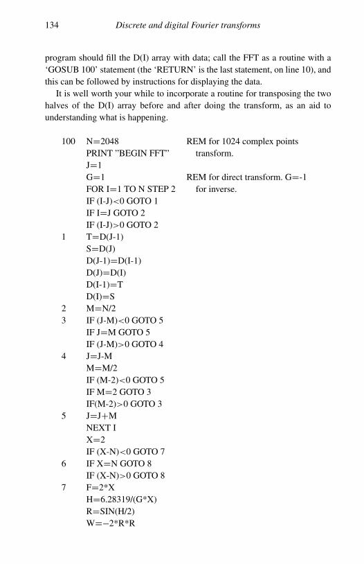
134 Discrete and digital Fourier transforms
program should fill the D(I) array with data; call the FFT as a routine with a‘GOSUB 100’ statement (the ‘RETURN’ is the last statement, on line 10), andthis can be followed by instructions for displaying the data.
It is well worth your while to incorporate a routine for transposing the twohalves of the D(I) array before and after doing the transform, as an aid tounderstanding what is happening.
100 ND2048 REM for 1024 complex pointsPRINT ”BEGIN FFT” transform.JD1GD1 REM for direct transform. GD-1FOR ID1 TO N STEP 2 for inverse.IF (I-J)<0 GOTO 1IF IDJ GOTO 2IF (I-J)>0 GOTO 2
1 TDD(J-1)SDD(J)D(J-1)DD(I-1)D(J)DD(I)D(I-1)DTD(I)DS
2 MDN/23 IF (J-M)<0 GOTO 5
IF JDM GOTO 5IF (J-M)>0 GOTO 4
4 JDJ-MMDM/2IF (M-2)<0 GOTO 5IF MD2 GOTO 3IF(M-2)>0 GOTO 3
5 JDJCMNEXT IXD2IF (X-N)<0 GOTO 7
6 IF XDN GOTO 8IF (X-N)>0 GOTO 8
7 FD2*XHD6.28319/(G*X)RDSIN(H/2)WD�2*R*R

9.4 A BASIC FFT routine 135
VDSIN(H)PD1QD0FOR MD1 TO X STEP 2FOR IDM TO N STEP FJDICXTDP*D(J-1)-Q*D(J)SDP*D(J)CQ*D(J-1)D(J-1)DD(I-1)-TD(J)DD(I)-SD(I-1)DD(I-1)CTD(I)DD(I)CSNEXT ITDPPDP*W-Q*VCPQDQ*WCT*VCQNEXT MXDFGOTO 6
8 CLSFOR ID0 TO N-1D(I)DD(I)/(SQR(N/2))NEXT IPRINT ”FFT DONE”
10 RETURN
Next, here is a short program to generate a file with .DAT extension whichwill contain a top-hat function of any width you choose. The data are generatedin ASCII and can be used directly with the FFT program above.
REM Program to generate a “Top-hat” function.INPUT “input desired file name”, A$INPUT ‘Top-hat Half-width ?’, NPID3.141 592 654DIM B(2047)FOR ID1024-N TO 1024CN STEP 2B(I)D1/(2�N)NEXT IC$D“.DAT”C$DA$CC$PRINT

136 Discrete and digital Fourier transforms
OPEN C$ FOR OUTPUT AS #1FOR ID0 TO 2047PRINT #1,B(I)NEXT ICLOSE #1
The simple file-generating arithmetic in lines 6–8 can obviously be replacedby something else, and this sort of ‘experiment’ is of great help in understandingthe FFT process.
The file thus generated can be read into the FFT program with the following:
REM Subroutine FILELOADREM To open a file and load contents into D(I)GOSUB 24(insert the next stage of the program, e.g. ‘GOSUB 100’, here)CLS:LOCATE 10,26,0PRINT “NAME OF DATA FILE ?”LOCATE 14,26,0INPUT A$ON ERROR GOTO 35OPEN “I”,#1,A$FOR ID0 TO 2047ON ERROR GOTO 35INPUT #1,D(I)NEXT ICLOSE
35 RETURN

Appendix
A.1 Parseval’s theorem and Rayleigh’s theorem
Parseval’s theorem states that∫ 1
�1
f (x)g�(x)dx D
∫ 1
�1
F (p)G�(p)dp.
This proof relies on the fact that if
g(x) D∫ 1
�1
G(p)e2πipx dp
then
g�(x) D∫ 1
�1
G�(p)e�2πipx dp
(simply by taking complex conjugates of everything).Then it follows that
G�(p) D∫ 1
�1
g�(x)e2πipx dx.
The argument of the integral on the left-hand side of the theorem can nowbe written as
f (x)g�(x) D∫ 1
�1
F (q)e2πiqx dq
∫ 1
�1
G�(p)e�2πipx dp.
We integrate both sides with respect to x. If we choose the order of integrationcarefully, we find∫ 1
�1
f (x)g�(x)dx D
∫ 1
�1
{∫ 1
�1
F (q)
[∫ 1
�1
G�(p)e�2πipx dp
]e2πiqx dq
}dx
137

138 Appendix
and, on changing the order of integration,
D
∫ 1
�1
{F (q)
∫ 1
�1
g�(x)e2πiqx dx
}dq
D
∫ 1
�1
F (q)G�(q)dq.
The theorem is often seen in a simplified form, with g(x) D f (x) andG(p) D F (p). Then it is written∫ 1
�1
jf (x)j2 dx D
∫ 1
�1
jF (p)j2 dp.
This is Rayleigh’s theorem.Another version of Parseval’s theorem involves the coefficients of a Fourier
series. In words, it states that the average value of the square of F (t) over oneperiod is the sum of the squares of all the coefficients of the series.
The proof, using the half-range series, is simple:
F (t) DA0
2C
1∑0
An cos
(2πnt
T
)C Bn sin
(2πnt
T
)
and, since all cross-products vanish on integration and
∫ T
0cos2(2πnt)dt D
∫ T
0sin2(2πnt)dt D
1
2,
we have
∫ T
0[F (t)]2 dt D T
[A2
0
4C
1∑1
A2n C B2
n
2
].
A.2 Useful formulae from Bessel-function theory
The Jacobi expansion
eix cos y D J0(x)C 21∑
nD1
inJn(x)cos(ny),
eix sin y D
1∑zD�1
Jz(x)eizy .

Appendix 139
The integral expansion
J0(2πρr) D1
2π
∫ 2π
0e2πiρr cos θ dθ,
which is a particular case of the general formula
Jn(x) Di�n
2π
∫ 2π
0einθ eix cos θ dθ,
d
dx
(xnC1JnC1(x)
)D xnC1Jn(x).
The Hankel transformThis is similar to a Fourier transform, but with polar coordinates, r, θ . TheBessel functions form a set with orthogonality properties similar to those ofthe trigonometrical functions and there are similar inversion formulae. Theseare
F (x) D∫ 1
0pf (p)Jn(px)dp,
f (p) D∫ 1
0xF (x)Jn(px)dx,
where Jn is a Bessel function of any order.Bessel functions are analogous in many ways to the trigonometrical func-
tions sine and cosine. In the same way as sine and cosine are the solutionsof the SHM equation d2y/dx2 C k2y D 0, they are the solutions of Bessel’sequation, which is
x2 d2y
dx2C x
dy
dxC (x2 � n2)y D 0.
In its full glory, n need not be an integer and neither x nor n need be real.The functions are tabulated in various books1 for real x and for integer andhalf-integer n, and can be calculated numerically, as are sines and cosines, bycomputer.
In its simpler form, as shown, the Hankel transform occurs with θ as variablewhen Laplace’s equation is solved in cylindrical polar coordinates and variablesare separated to give functions R(r)�(θ )�(φ), and this is why it proves usefulin Fourier transforms with circular symmetry.
1 For example, in Jahnke & Emde (see the bibliography).

140 Appendix
A.3 Conversion of Fourier-series coefficients into complexexponential form
We use de Moivre’s theorem to do the conversion. Write 2πν0t as θ . Then,expressed as a half-range series, F (t) becomes
F (t) D A0/2C1∑
mD1
Am cos(mθ )C Bm sin(mθ ).
This can also be written as a full-range series:
F (t) D1∑
mD�1
am cos(mθ )C bm sin(mθ ),
where Am D am C a�m and Bm D bm � b�m.Then, by virtue of de Moivre’s theorem, the full-range series becomes
F (t) D1∑
mD�1
am
2(eimθ C e�imθ )C
bm
2i(eimθ � e�imθ )
D
1∑mD�1
am � ibm
2eimθ C
1∑mD�1
am C ibm
2e�imθ .
The two sums are independent and m is a dummy suffix, which means thatit can be replaced by any other suffix not already in use. Here, we replacem D �m in the second sum. Then
F (t) D1∑
mD�1
am � ibm
2eimθ C
1∑mD�1
a�m C ib�m
2eimθ
D
1∑mD�1
eimθ
{Am � iBm
2
}
D
1∑mD�1
eimθCm
and C�m D C�m.

Bibliography
The most popular books on the practical applications of Fourier theory areundoubtedly those of Champeney and Bracewell, and they cover the presentground more thoroughly and in much more detail than here. E. Oran Brigham,on the fast Fourier transform (FFT), is the classic work on the subjects dealtwith in Chapter 9.
Of the more theoretical works, the ‘bible’ is Titchmarsh, but a more readable(and entertaining) work is Korner’s. Whittaker’s (not to be confused with themore prolific E. T. Whittaker) is a specialized work on interpolation, but thatis a subject which is getting more and more important, especially in computergraphics.
Many writers on quantum mechanics, atomic physics and electronic engi-neering like to include an early chapter on Fourier theory. One or two (whoshall be nameless) get it wrong! They confuse ω with ν or leave out a 2π whenthere should be one, or something like that. The specialist books, like thosebelow, are much to be preferred.
Abramowitz, M. & Stegun, I. A. Handbook of Mathematical Functions. Dover, NewYork. 1965A more up-to-date version of Jahnke & Emde, below.
Bracewell, R. N. The Fourier Transform and its Applications. McGraw–Hill, New York.1965This is one of the two most popular books on the subject. Similar in scope to thisbook, but more thorough and comprehensive.
Brigham, E. O. The Fast Fourier Transform. Prentice Hall, New York. 1974The standard work on digital Fourier transforms and their implementation byvarious kinds of FFT program.
Champeney, D. C. Fourier Transforms and Their Physical Applications. AcademicPress, London & New York. 1973Like Bracewell, one of the two most popular books on practical Fourier transform-ing. Covers similar ground, but with some differences in detail.
141
142 Bibliography
Champeney, D. C. A Handbook of Fourier Theorems. Cambridge University Press,Cambridge. 1987
Herman, G. T. Image Reconstruction from Projections. Academic Press, London & NewYork. 1980Includes details of Fourier methods (among others) for computerized tomography,including theory and applications.
Jahnke, E. & Emde, F. Tables of Functions with Formulae and Curves. Dover, NewYork. 1943The classic work on the functions of mathematical physics, with diagrams, chartsand tables of Bessel functions, Legendre polynomials, spherical harmonics etc.
Korner, T. W. Fourier Analysis. Cambridge University Press, Cambridge. 1988One of the more thorough and entertaining works on analytic Fourier theory, butplenty of physical applications: expensive, but firmly recommended for seriousstudents.
Titchmarsh, E. C. An Introduction to the Theory of Fourier Integrals. Clarendon Press,Oxford. 1962The theorists’ standard work on Fourier theory. Unnecessarily difficult for ordinarymortals, but needs consulting occasionally.
Watson, G. N. A Treatise of the Theory of Bessel Functions. Cambridge UniversityPress, Cambridge. 1962Another great theoretical classic: chiefly for consultation by people who haveequations they can’t solve, and which seem likely to involve Bessel functions.
Whittaker, J. M. Interpolary Function Theory. Cambridge University Press, Cambridge.1935A slim volume dealing with (among other things) the sampling theorem and prob-lems of interpolating points between samples of band-limited curves.
Wolf, E. Introduction to the Theory of Coherence and Polarization of Light. CambridgeUniversity Press, Cambridge. 2007Gives more detail about material in Chapter 3, especially regarding coherence andthe van Cittert–Zernike theorem.
Index
f refers to footnote.
addition theorem 22Airy disc 100, 102aliasing 34amplitude 6
coefficients 7diffracted 42in Fourier transforms 8of harmonics 4modulation 72
analytic expansion 5signal 42f, 60wave vector 60
angular frequency 10measure 10
annulus 100antenna
design 56end-fire 56
antisymmetrical 11, 19, 120 et seq.aperture
function 42with phase changes 51
apodizing 50, 57fapodizing masks, 50 et seq.Argand diagram 11associative rule, convolutions 25antisymmetry 120 et seq.autocorrelation
function 68theorem 29
Babinet’s principle 54bandwidth, channel 68, 73, 74, 80, 82BASIC program for FFT 133baud-rate 74bed-of-nails 115
Beer’s law 111Bessel functions 74, 75, 99
Jacobi expansion in 75, 138Bessel’s equation 139bit-reversed order 131blaze
angle 54wavelength 54
blazing of diffraction gratings 53box-car function 11fBreit–Wigner formula 93
cardinal theorem, interpolary function theory,33
Cartesian coordinates 97Cauchy’s integral formula 84circular symmetrycoherence 58
coefficient 61degree of 61length 59partial, and fringe visibility 60
communication channel 66commutative rule, convolutions 25complex exponentials 7, 140computerized axial tomography 108 et seq.conjugate variables 10Connes’ apodizing function 91convolutions 22 et seq.
algebra of 30of two delta-functions 30of two Gaussians 27, 28
convolution theorem 26derivative theorem 32
contour integration 83Cooley–Tukey algorithm 128
143

144 Index
damped oscillator 91, 92damping
coefficient, 92constant, Planck’s 91
decay, exponential 14deconvolution 49de l’Hopital’s rule 6fde Moivre’s theorem 7, 140delta-function, Dirac 15
convolution of two 31convolution with 27parallel-plane 116
derivative theorem 31diffraction
aperture with prism 52, 53Fraunhofer 40grating, transmission 46
blazed 53intensity distribution of 48resolution of 49
single slit 44three slits 46two slits 45
dipolearrays 55 et seq.moment 91radiation, power of 91transitions 93
Dirichletconditions 20, 21, 38, 66function 20f
Diracbed of nails 115comb 17, 18, 47, 53, 75delta-function, defined 15
Fourier transform of 16fence 114point arrays 118spike 112wall 105 et seq.
discrete Fourier transform 128matrix form of 129
distributive rule, convolutions25
Doppler broadening 95
end-fire arrays 56electric charge, accelerated 91eriometer, Young’s 55error, periodic, in grating ruling
75
exponential decay 14, 96exponentials, complex 7, 9
Fabry–Perot etalon 57fringes and Lorentz profile 96
fast Fourier transform (FFT)BASIC routine for 133history of 127
filter 69low-pass 80matched, theorem 70
folding frequency 33Fourier
coefficients 8inversion theorempairs 9series 2, 6, 7, 8, 17synthesizer 82
Fourier transformsdigital 127 et seq.
history of 127fdiscrete 128
matrix form 129formal complex 120 et seq.modular 1, 64, 120multi-dimensional 105phase 120power 120two-dimensional 97, 132
in polar coordinates 98with circular symmetry 100without circular symmetry 103
Fraunhofer diffraction 40 et seq.two-dimensional 101
by circular aperture 102by rectangular slot 101
frequencyangular 10folding 33fundamental 1modulation 73spectrum 70
fringe visibility 60, 61defined 61
FWHM (width parameter) 13, 94, 95
Gaussianfunction 13, 16profile 95
ghosts, Rowland 76Gibbs phenomenon 81

Index 145
Green’s function 24graphical representation
half-width, Gaussian 96Hankel transforms 98, 139harmonics 1, 6
amplitude of 4harmonic oscillator, damped 92 et seq.Hartley–Shannon theorem 74Hermitian functions 126Heaviside step function 77 et seq.history, discrete transforms 127fHuygens’ principle 40
wavelets 52
impulse response 24intensity
in a diffraction grating 48in single-slit diffraction 43of a wave 43
interference spectrometry 86interferogram 90interferometer, Michelson 87interferometry, fundamental formula 86interpolary function theory 33interpolation theorem 35interval, sampling 33instrumental function 23inverse transform 9inversion formulae 7
Hankel transform 99
Jacobi expansion 75, 138jinc-function 100Johnson noise 68
Kronecker-delta 99
lattices 119lifetime of an excited state 93line shapes, spectral 49, 86, 91, 96line width, natural 93Lorentz profile 14, 94
and Fabry–Perot fringes 96low-pass filter 80, 82
matched-filter theorem 70Maxwellian velocity distribution 94Michelson
interferometer 86stellar interferometer 61 et seq.
Michelson and Stratton harmonic integrator82
Miller indices 119modular transformmodulating signalmodulations 71modulation
amplitude 72frequency 73index 74pulse-height 76pulse-width 76
multiplex advantage 88transmission 77
multiplex spectrometer 86multiplex transmission 77multiplexing
frequency 77time 77
nail, Dirac 112pair of 113
noise 68filters 69 et seq.Johnson 68photo-electron shot 69semi-conductor 69white 68
Nyquist diagram 69, 124frequency 33
oblique incidence 43, 44orthogonality
of Bessel functions 139of sines and cosines 4
overtones 1
Parseval’s theorem 32, 67periodic errors 75phase 6f
angle 1f, 60, 69, 96fchange 40fand coherence 58difference 6, 7, 42transform 120
Planck, M. 91point arrays 118point-spread function 24polar coordinates 98
diagrams 58power spectrum, see spectral power density

146 Index
profileGaussian 95instrumental 91line 14Lorentz 14, 93
projection 108slice theorem 110
pulse-train, passage through a filter 82
radiation damping 91Radon transform 108, 109
projection slice theorem 110Rayleigh, Lord 88Rayleigh criterion 103Rayleigh’s theorem 32, 67
in two dimensions 99reciprocal lattice 117, 119rect function 11fresolution, difraction gratingRowland ghosts 76
sampling 77frequency 35rate 34, 77theorem 33under- 35
saw-tooth waveform 19Schwartz’s inequality 71serial link 77sgn function 78shah (Ш )-function 17shift theorem 22, 27, 67signal analysis 66 et seq.signal/noise ratio 69, 74similarity theorem 36sinc-function 12, 44sinusoid, convolution with 38spectral
lines, shapes of 49, 86, 91, 96power density (SPD) 89, 90, 93, 95
spectrometer, perfect 22, 23spike, two-dimensional, FT of 112square-wave 5Stratton, Michelson and, harmonic integrator
82sub-carrier 77superposition of planes 108symmetry 120 et seq.
temperature broadening 95theorems
addition 22autocorrelation 29cardinal, of interpolary function theory
33convolution 26
derivative 32in two-dimensional FTs 99
de Moivre’s 7, 140derivative 31Fourier inversion 9matched filter 70Parseval’s 32, 67, 137power 32projective slice 110Rayleigh’s 32, 137sampling 33similarity 36
in two-dimensional FTs 99shift 22, 27, 67
in two-dimensional FTs 99Van Cittert–Zernike 64Wiener–Khinchine 67
tomography, computer axial 108top-hat function 11, 31
in two-dimensional FT’s 100transition probablity 93triangle function 28twiddle factors 131
Van Cittert–Zernike theorem 64variables
abstract 9conjugate 10physical 9
velocity distribution, Maxwell 95visibility of fringes 60, 61Voigt profile 95
separation of components 95voltage-step, passage through a filter 80
waveformdouble sawtooth 38rectangular 5, 37
wavenumber 88, 90width parameter (FWHM) 13, 14, 95Witch of Agnesi 14fWiener–Khinchine theorem 67
Yagi aerial 56Young’s slits 64
interferometer 61


![[This page intentionally left blank.] - Regina](https://static.fdocuments.in/doc/165x107/61b424db652c60231a4f25af/this-page-intentionally-left-blank-regina.jpg)