http://www.cambridge.org/9780521888868

ii

This page intentionally left blank

ESTUARIES

This volume provides researchers, students, practising engineers and managersaccess to state-of-the-art knowledge, practical formulae and new hypotheses forthe dynamics, mixing, sediment regimes and morphological evolution in estuaries.The objectives are to explain the underlying governing processes and synthesise

these into descriptive formulae which can be used to guide the future developmentof any estuary. Each chapter focuses on different physical aspects of the estuarinesystem – identifying key research questions, outlining theoretical, modelling andobservational approaches, and highlighting the essential quantitative results. Thisallows readers to compare and interpret different estuaries around the world, anddevelop monitoring and modelling strategies for short-term management issues andfor longer-term problems, such as global climate change.The book is written for researchers and students in physical oceanography and

estuarine engineering, and serves as a valuable reference and source of ideas forprofessional research, engineering and management communities concerned withestuaries.

DAVID PRANDLE is currently Honorary Professor at the University of Wales’School of Ocean Sciences, Bangor. He graduated as a civil engineer from theUniversity of Liverpool and studied the propagation of a tidal bore in the RiverHooghly for his Ph.D. at the University of Manchester. He worked for 5 years as aconsultant to Canada’s National Research Council, modelling the St. Lawrence andFraser rivers. He was then recruited to the UK’s Natural Environment ResearchCouncil’s Bidston Observatory to design the operational software for controlling theThames Flood Barrier. He has subsequently carried out observational, modellingand theoretical studies of tide and storm propagation, tidal energy extraction,circulation andmixing, temperatures and water quality in shelf seas and their coastalmargins.

ESTUARIES

Dynamics, Mixing, Sedimentation and Morphology

DAVID PRANDLEUniversity of Wales, UK

CAMBRIDGE UNIVERSITY PRESS

Cambridge, New York, Melbourne, Madrid, Cape Town, Singapore, São Paulo

Cambridge University Press

The Edinburgh Building, Cambridge CB2 8RU, UK

First published in print format

ISBN-13 978-0-521-88886-8

ISBN-13 978-0-511-48101-7

© Jacqueline Broad and Karen Green 2009

2009

Information on this title: www.cambridge.org/9780521888868

This publication is in copyright. Subject to statutory exception and to the

provision of relevant collective licensing agreements, no reproduction of any part

may take place without the written permission of Cambridge University Press.

Cambridge University Press has no responsibility for the persistence or accuracy

of urls for external or third-party internet websites referred to in this publication,

and does not guarantee that any content on such websites is, or will remain,

accurate or appropriate.

Published in the United States of America by Cambridge University Press, New York

www.cambridge.org

eBook (NetLibrary)

hardback

Contents

List of symbols page viii1 Introduction 1

1.1 Objectives and scope 11.2 Challenges 31.3 Contents 51.4 Modelling and observations 131.5 Summary of formulae and theoretical frameworks 16Appendix 1A 17References 21

2 Tidal dynamics 232.1 Introduction 232.2 Equations of motion 242.3 Tidal response – localised 262.4 Tidal response – whole estuary 312.5 Linearisation of the quadratic friction term 382.6 Higher harmonics and residuals 402.7 Surge–tide interactions 442.8 Summary of results and guidelines for application 46References 48

3 Currents 503.1 Introduction 503.2 Tidal current structure – 2D (X-Z) 533.3 Tidal current structure – 3D (X-Y-Z) 593.4 Residual currents 673.5 Summary of results and guidelines for application 71Appendix 3A 73Appendix 3B 75References 76

v

4 Saline intrusion 784.1 Introduction 784.2 Current structure for river flow, mixed and stratified saline

intrusion 844.3 The length of saline intrusion 904.4 Tidal straining and convective overturning 964.5 Stratification 1054.6 Summary of results and guidelines for application 108Appendix 4A 111References 120

5 Sediment regimes 1235.1 Introduction 1235.2 Erosion 1265.3 Deposition 1295.4 Suspended concentrations 1315.5 SPM time series for continuous tidal cycles 1355.6 Observed and modelled SPM time series 1375.7 Summary of results and guidelines for application 142Appendix 5A 145References 149

6 Synchronous estuaries: dynamics, saline intrusion and bathymetry 1516.1 Introduction 1516.2 Tidal dynamics 1526.3 Saline intrusion 1586.4 Estuarine bathymetry: theory 1616.5 Estuarine bathymetry: assessment of theory against

observations 1656.6 Summary of results and guidelines for application 170References 173

7 Synchronous estuaries: sediment trapping and sorting – stablemorphology 1757.1 Introduction 1757.2 Tidal dynamics, saline intrusion and river flow 1797.3 Sediment dynamics 1827.4 Analytical emulator for sediment concentrations and fluxes 1847.5 Component contributions to net sediment flux 1877.6 Import or export of sediments? 1937.7 Estuarine typologies 1967.8 Summary of results and guidelines for application 199References 202

vi Contents

8 Strategies for sustainability 2058.1 Introduction 2058.2 Model study of the Mersey Estuary 2068.3 Impacts of GCC 2188.4 Strategies for modelling, observations and monitoring 2238.5 Summary of results and guidelines for application 226Appendix 8A 228References 231Index 234

Contents vii

Symbols

A cross-sectional areaB channel breadthC concentration in suspensionD water depthE vertical eddy viscosity coefficientEX tidal excursion lengthF linearised bed friction coefficient

dimensionless friction termH total water depth D + ςIF sediment in-fill timeJ dimensionless bed friction parameterKz vertical eddy diffusivity coefficientL estuary lengthLI salinity intrusion lengthLM resonant estuarine lengthM2 principal lunar semi-diurnal tidal constituentM4 M6 over-tides of M2

MS4 MSf over-tides of M2 and S2P tidal periodQ river flowRI Richardson numberSR Strouhal number U*P/DSc Schmid number (Kz/E)St Stratification numberSX relative axial salinity gradient 1/ρ ∂ρ/∂xS dimensionless salinity gradientSL axial bed slopeSP spacing between estuaries

viii

TF flushing timeU axial currentU* tidal current amplitude

Residual current components:U0 river flowUs density-inducedUw wind-inducedV lateral currentW vertical currentWs sediment fall velocityX axial dimensionY lateral axisZ vertical axisc wave celerityd particle diameterf bed friction coefficient (�0.0025)g gravitational constanti (−1)½

surface slopek wave number (2π/λ)m power of axial depth variations (xm)n power of axial breadth variation (xn)s salinityt timet50 half-life of sediment in suspension (α/0.693)y dimensionless distance from mouthz = Z/Dα exponential deposition rate

exponential breadth variation (eαx)tan α side slope gradient (B/2D)β exponential suspended sediment profile

exponential depth variation (eβx)γ sediment erosion coefficientε efficiency of mixingς surface elevationς* tidal elevation amplitudeθ phase advance of ζ* relative to U*λ wavelengthν funnelling parameter (n + 1)/(2 − m)

Symbols ix

π 3.141592ρ densityσ frequencyτ stressφ latitudeφE potential energy anomalyψ ellipse directionω tidal frequency (P/2π)Ω Coriolis parameter (2ωs sinφ)

Superscripts* tidal amplitude– depth mean

Subscripts0 residual1D, 2D, 3D one-, two- and three-dimensional

Note: other notations are occasionally used locally for consistency with referencedpublications. These are defined as they appear.

x Symbols

1

Introduction

1.1 Objectives and scope

This book aims to provide students, researchers, practising engineers and managersaccess to state-of-the-art knowledge, practical formulae and new hypotheses cover-ing dynamics, mixing, sediment regimes and morphological evolution in estuaries.Many of these new developments assume strong tidal action; hence, the emphasis is onmeso- and macro-tidal estuaries (i.e. tidal amplitudes at the mouth greater than 1m).For students and researchers, this book provides deductive descriptions of the-

oretical derivations, starting from basic dynamics through to the latest researchpublications. For engineers and managers, specific developments are presented inthe form of new formulae encapsulated within generalised Theoretical Frameworks.Each chapter is presented in a ‘stand-alone’ style and ends with a concise

‘Summary of Results and Guidelines for Application’ outlining the issues involved,the approach, salient results and how these can be used in practical terms. The goalthroughout is to explain governing processes in a generalised form and synthesiseresults into guideline Frameworks. These provide perspectives to interpret and inter-compare the history and conditions in any specific estuary against comparableexperience elsewhere. Thus, a background can be established for developing mon-itoring strategies and commissioning of modelling studies to address immediateissues alongside longer-term concerns about impacts of global climate change.

1.1.1 Processes

Estuaries are where ‘fresh’ river water and saline sea water mix. They act as bothsinks and sources for pollutants depending on (i) the geographical sources of thecontaminants (marine, fluvial, internal and atmospheric), (ii) their biological andchemical nature and (iii) with temporal variations in tidal amplitude, river flow,seasons, winds and waves.

1

Tides, surges and waves are generally the major sources of energy input intoestuaries. Pronounced seasonal cycles often occur in temperature, light, waves, riverflows, stratification, nutrients, oxygen and plankton. These seasonal cycles alongsideextreme episodic events may be extremely significant for estuarine ecology. As anexample, adjustments in axial intrusion of sea water and variation in vertical stratifica-tion associated with salinity and temperature may lead to rapid colonisation or,conversely, extinction of sensitive species. Likewise, changes to the almost impercep-tible larger-scale background circulations may affect the pathways and hence lead toaccumulation of persistent tracers. Dyer (1997) provides further descriptions of theseprocesses alongside useful definitions of much of the terminology used in this book.Vertical and horizontal shear in tidal currents generate fine-scale turbulence,

which determines the overall rate of mixing. However, interacting three-dimensional(3D) variations in the amplitude and phase of tidal cycles of currents and contaminantsseverely complicate the spatial and temporal patterns of tracer distributions andthereby the associated mixing. On neap tides, near-bed saline intrusion may enhancestability, while on springs, enhanced near-surface advection of sea water can lead tooverturning. Temperature gradients may also be important; solar heating stabilises thevertical density profile, while winds promote surface cooling which can produceoverturning. In highly turbid conditions, density differences associatedwith suspendedsediment concentrations can also be important in suppressing turbulent mixing.The spectrum of tidal energy input is effectively constrained within a few tidal

constituents, and, in mid-latitudes, the lunar M2 constituent is generally greater thanthe sum of all others – providing a convenient basis for linearisation of the equationsfor tidal propagation. However, ‘mixing’ involves a wider spectrum of interactingnon-linear processes and is thus more difficult to simulate. The ‘decay time’ fortidal, surge, wave and associated turbulent energy in estuaries is usually measured inhours. By contrast, the flushing time for river inputs generally extends over days.Hence, simulation of the former is relatively independent of initial conditions, whilesimulation of the latter is complicated by ‘historical’ chronology resulting inaccumulation of errors.

1.1.2 Historical developments

Following the end of the last ice age, retreating ice cover, tectonic rebound and therelated rise in mean sea level (msl) resulted in receding coastlines and consequentmajor changes in both the morphology and the dynamics of estuaries. Large post-glacial melt-water flows gouged deep channels with the rate of subsequent in-fillingdependent on localised availability of sediments. Deforestation and subsequentchanges in farming practices substantially changed the patterns of river flows andboth the quantity and the nature of fluvial sediments. Thus, present-day estuarine

2 Introduction

morphologies reflect adjustments to these longer-term, larger-scale effects along-side more recent, localised impacts from urban development and engineering‘interventions’.Ports and cities have developed on almost all major estuaries, exploiting oppor-

tunities for both inland and coastal navigation, alongside supplies of freshwater andfisheries. In more recent times, the scale of inland navigation has generally declinedand the historic benefit of an estuary counterbalanced by growing threats of flood-ing. Since estuaries often supported major industrial development, the legacy ofcontaminants can threaten ecological diversity and recreational use. The spread ofnational and international legislation relating to water quality can severely restrictdevelopment, not least because linking discharges with resulting concentrations isinvariably complicated by uncertain contributions from wider-area sources andhistorical residues. This combination of legal constraints and uncertainties aboutimpacts from future climate changes threatens planning-blight for estuarine devel-opment. This highlights the need for clearer understanding of the relative sensitivityof estuaries to provide realistic perspectives on their vulnerability to change.

1.2 Challenges

Over the next century, rising sea levels at cities bordering estuaries may requiremajor investment in flood protection or even relocation of strategic facilities. Theimmediate questions concern the changing magnitudes of tides, surges and waves.However, the underlying longer-term (decadal) issue is how estuarine bathymetrieswill adjust to consequent impacts on these dynamics (Fig. 1.1; Prandle, 2004). Inaddition to the pressing flood risk, there is growing concern about sustainableexploitation of estuaries. A common issue is how economic and natural environmentinterests can be reconciled in the face of increasingly larger-scale developments.

1.2.1 Evolving science and technology agendas

Before computers became available, hydraulic scale models were widely used tosimulate dynamics and mixing in estuaries. The scaling principles were based onmaintaining the ratios of the leading terms in the equation describing tidal propaga-tion. Ensuing model ‘validation’ was generally limited to reproduction of tidalheights along the estuary. Subsequent expansion in observational capabilities indi-cated how difficulties arose when such models were used to study saline intrusion,sediment regimes and morphological adjustments.Even today, validation of sophisticated 3D numerical models may be restricted to

simulation of an M2 cycle – providing little guarantee of accurate reproduction ofhigher harmonics or residual features. Likewise, these fine-resolution 3D models

1.2 Challenges 3

may encounter difficulties in reproducing the complexity and diversity of mixingand sedimentary processes. Moreover, the paucity of observational data invariablylimits interpretation of sensitivity tests. However, modelling is relatively cheap andcontinues to advance rapidly, whilst observations are expensive and technologydevelopments often take decades. Thus, a major challenge in any estuary study ishow to use theory to bridge the gaps between modelling and available observations.Both historical and ‘proxy’ data must be exploited, e.g. wave data constructed fromwind records, flood statistics from adjacent locations, sedimentary records of floraand fauna as indicators of saline intrusion and anomalous fossilised bed features asevidence of extreme events.The evolving foci for estuarine research are summarised in Fig. 1.2. These have

evolved alongside successive advances in theory, modelling and observationaltechnologies to address changing political agendas.

1.2.2 Key questions

Successive chapters address the following sequence of key questions:

(Q1) How can strategies for sustainable exploitation of estuaries be developed?(Q2) How do tides in estuaries respond to shape, length, friction and river flow? Why are

some tidal constituents amplified yet others reduced and why does this vary from oneestuary to another?

Tidessurgeswavesmean sea levels

Sediment sourcesink

Dredging

Bank & marshexchange

Underlying geology

River flowfluvial load

Coring

Surficial sediments

Reclamation

Fig. 1.1. Schematic of major factors influencing estuarine bathymetry.

4 Introduction

(Q3) How do tidal currents vary with depth, friction, latitude and tidal period?(Q4) How does salt water intrude and mix and how does this change over the cycles of

Spring–Neap tides and flood-to-drought river flows?(Q5) How are the spectra of suspended sediments determined by estuarine dynamics?(Q6) What determines estuarine shape, length and depth?(Q7) What causes trapping, sorting and high concentrations of suspended sediments?

How does the balance of ebb and flood sediment fluxes adjust to maintain bathymetricstability?

(Q8) How will estuaries adapt to Global Climate Change?

1.3 Contents

1.3.1 Sequence

The chapters follow a deductive sequence describing (2) Tidal Dynamics,(3) Currents, (4) Saline Intrusion, (5) Sediment Regimes, (6) Synchronous Estuary:Dynamics, Saline Intrusion and Bathymetry, (7) Synchronous Estuary: SedimentTrapping and Sorting – Stable Morphology and (8) Strategies for Sustainability.Analytical solutions for the first-order dynamics of estuaries are derived in Chapter 2and provide the basic framework of our understanding. Details of associatedcurrents are described in Chapter 3. Tidal currents and elevations in estuaries arelargely independent of biological, chemical and sedimentary processes – except fortheir influences on the bed friction coefficient. Conversely, these latter processes aregenerally highly dependent on tidal motions. Thus, in Chapters 4 and 5, we considerhow estuarine mixing and sedimentation are influenced by tidal action. Chapters 6and 7 apply these theories to synchronous estuaries, yielding explicit algorithms

Tidegauges

TidesStormsurges

WavesT emperaturesalinity

Sedimentsalgal blooms

primary productivity

Fish stocks

Ecologicalcommunities

NavigationCoastaldefence

Offshoreindustries

Agriculture(marine & terrestr ial)

T ourism

Sustainableexploitation

Defence

19901980 20102000

MeteorologyIn situtelemetry

SatelliteAircraftradarferries

Fig. 1.2. Historical development in key processes, ‘end-users’ and observationaltechnologies.

1.3 Contents 5

for tidal currents, estuarine lengths and depths, sediment sorting and trapping and abathymetric framework based on tidal amplitude and river flow.

1.3.2 Tidal dynamics

Chapter 2 examines the propagation of tides, generated in ocean basins, intoestuaries, explaining how and why tidal elevations and currents vary within estu-aries (Fig. 1.3; Prandle, 2004). The mechanisms by which semi-diurnal and diurnalconstituents of ocean tides produce additional higher-harmonic and residual com-ponents within estuaries are illustrated. Since the expedient of linearising therelevant equations in terms of a predominant (M2) constituent is extensively usedthroughout this book, the details of this process are described. Many earlier textsand much of the literature focus on large, deep estuaries with relatively low frictioneffects. Here, it is indicated how to differentiate between such deep estuaries andshallower frictionally dominated systems and the vast differences in their responsecharacteristics are illustrated.

2ν

3 4 5

2.5

1.0

0.5

51030

5070

90

100

B

A

D G

IE

H

F

C

50

25

10

5.0

2.5

–180° –150°

150°90° 1.0

0.1

0.01

–10°

–1°

–30°

–90°

0.5

30°

050–30°

–90°

100

100

1

2

3

y4

5

6

7

Fig. 1.3. Tidal elevation responses for funnel-shaped estuaries. ν represents degreeof bathymetric funnelling and y distance from the mouth, y= 0. Dashed contoursindicate relative amplitudes and continuous contours relative phases. Lengths,y (for M2), and shapes, ν, for estuaries (A)–(I) shown in Table 2.1.

6 Introduction

1.3.3 Currents

Chapter 3 examines how tidal currents vary along (axially) and across estuariesand from surface to bed. Changes in current speed, direction and phase (timingof peak or slack values) are explained by decomposition of the tidal current ellipseinto clockwise and anti-clockwise rotating components. While the main focus ison explaining the nature and range of tidal currents, the characteristics of wind-and density-driven currents are also described. A particular emphasis is on derivingthe scaling factors which encapsulate the influence of the ambient environmentalparameters, namely depth, friction factor and Coriolis coefficient, i.e. latitude(Fig. 1.4; Prandle, 1982).

1.3.4 Saline intrusion

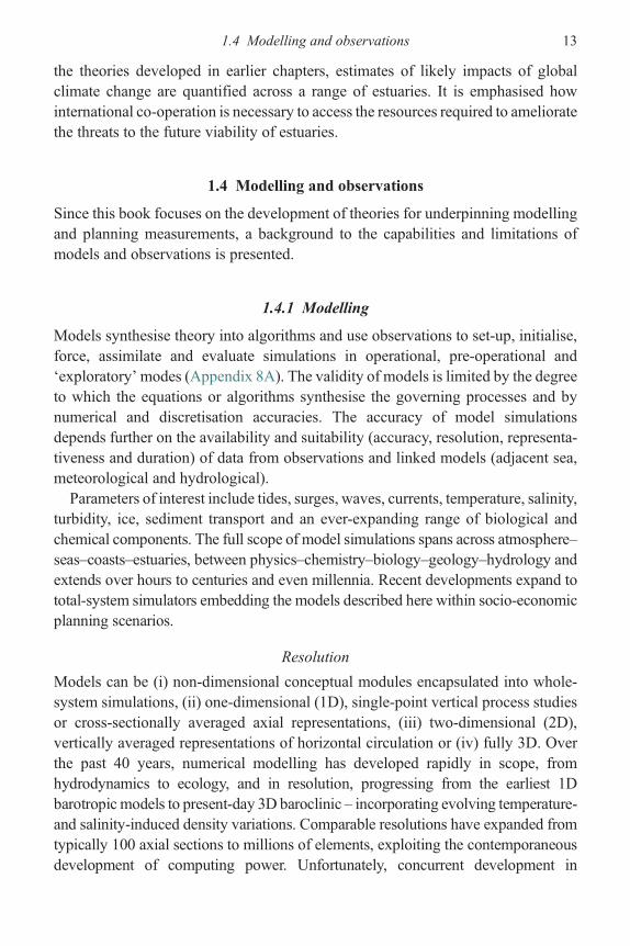
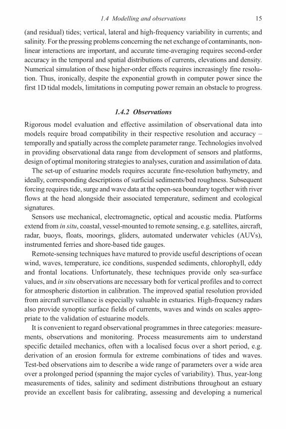
Noting the earlier definition of estuaries as regions where salt and fresh water mix,Chapter 4 examines the details of this mixing. It is shown how existing theoriesderived for saline intrusion in channels of constant cross section can be adaptedfor mixing in funnel-shaped estuaries. Saline intrusion undergoes simultaneousadjustments in axial location and mixing length – explaining traditional problemsin understanding observed variations over spring–neap and flood-drought condi-tions (Fig. 1.5; Liu et al., 2008).

Fig. 1.4. Vertical profiles of tidal current, U*(z)/U*mean, versus the Strouhalnumber, SR, U* tidal current amplitude, P tidal period, D depth, SR =U*P/D.

1.3 Contents 7

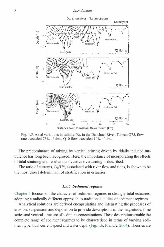
The predominance of mixing by vertical stirring driven by tidally induced tur-bulence has long been recognised. Here, the importance of incorporating the effectsof tidal straining and resultant convective overturning is described.The ratio of currents, U0/U*, associated with river flow and tides, is shown to be

the most direct determinant of stratification in estuaries.

1.3.5 Sediment regimes

Chapter 5 focuses on the character of sediment regimes in strongly tidal estuaries,adopting a radically different approach to traditional studies of sediment regimes.Analytical solutions are derived encapsulating and integrating the processes of

erosion, suspension and deposition to provide descriptions of the magnitude, timeseries and vertical structure of sediment concentrations. These descriptions enable thecomplete range of sediment regimes to be characterised in terms of varying sedi-ment type, tidal current speed and water depth (Fig. 1.6; Prandle, 2004). Theories are

Danshuei river – T ahan stream

–5

–10

–5

–5

0 20 302510 155

–10

–10

Dep

th (

m)

Dep

th (

m)

Dep

th (

m)

Salinity:ppt

Hsin-Hai Bri.

Hsin-Hai Bri.

Hsin-Hai Bri.

T aipei Bri.

T aipei Bri.

T aipei Bri.

Kuan-Du Bri.

Kuan-Du Bri.

Kuan-Du Bri.

River mouth

River mouth

River mouth

Q75 flo w

Qm flo w

Q10 flo w

Distance from Danshuei River mouth (km)

123456791113151719212223242527

29

3031323332

3128

24 2321 19

15

17 1311 9 7 6 5 13

302827

25 2220 18

1513

1412

1110

97

6 4 3 12

Fig. 1.5. Axial variations in salinity,‰, in the Danshuei River, Taiwan Q75, flowrate exceeded 75% of time, Q10 flow exceeded 10% of time.

8 Introduction

developed by which tidal analyses of suspended sediment time series, obtained fromeither model simulations or observations, can be used to explain the underlyingcharacteristics.

1.3.6 Synchronous estuary: dynamics, salineintrusion and bathymetry

A ‘synchronous estuary’ is where the sea surface slope due to the axial gradient inphase of tidal elevation significantly exceeds the gradient from changes in tidalamplitude. The adoption of this assumption in Chapters 6 and 7 enables the theoreticaldevelopments described in earlier chapters to be integrated into an analytical emu-lator, incorporating tidal dynamics, saline intrusion and sediment mechanics.Chapter 6 re-examines the tidal response characteristics for any specific locationwithin an estuary. The ‘synchronous’ assumption yields explicit expressions forboth the amplitude and phase of tidal currents and the slope of the sea bed.Integration of the latter expression provides an estimate of the shape and lengthof an estuary. By combining these results with existing expressions for the lengthof saline intrusion and further assuming that mixing occurs close to the seawardlimit, an expression linking depth at the mouth with river flow is derived. Hence,a framework for estuarine bathymetry is formulated showing how size and shapeare determined by the ‘boundary conditions’ of tidal amplitude and river flow(Fig. 1.7; Prandle et al., 2005).

Fig. 1.6. Spring–neap patterns of sediment concentrations at fractional heightsabove the bed.

1.3 Contents 9

1.3.7 Synchronous estuary: sediment trappingand sorting – stable morphology

Chapter 7 indicates how, in ‘synchronous’ estuaries, bathymetric stability is main-tained via a combination of tidal dynamics and ‘delayed’ settlement of sedimentsin suspension. An analytical emulator integrates explicit formulations for tidal andresidual current structures together with sediment erosion, suspension and deposi-tion. The emulator provides estimates of suspended concentrations and net sedimentfluxes and indicates the nature of their functional dependencies. Scaling analysesreveal the relative impacts of terms related to tidal non-linearities, gravitationalcirculation and ‘delayed’ settling.The emulator is used to derive conditions necessary to maintain zero net flux of

sediments, i.e. bathymetric stability. Thus, it is shown how finer sediments are importedand coarser ones are exported, with more imports on spring tides than on neaps,i.e. selective trapping and sorting and consequent formation of a turbidity maximum.The conditions derived for maintaining stable bathymetry extend earlier concepts offlood- and ebb-dominated regimes. Interestingly, these derived conditions correspondwith maximum sediment suspensions. Moreover, the associated sediment-fall veloci-ties are in close agreement with settling rates observed in many estuaries. Figure 1.8(Lane and Prandle, 2006) encapsulates these results, illustrating the dependency on

Fig. 1.7. Zone of estuarine bathymetry. Coordinates (Q, ς) for Coastal Plain andBar-Built estuaries, Q river Flow and ς elevation amplitude. Bathymetric zonebounded by Ex < L, LI < L and D/U3 < 50m2 s−3.

10 Introduction

delayed settlement (characterised by the half-life in suspension t50) and the phasedifference, θ, between tidal current and elevation. A feedback mechanism betweentidal dynamics and net sedimentation/erosion is identified involving an interactionbetween suspended and deposited sediments.These results from Chapters 6 and 7 are compared with observed bathymetric

and sedimentary conditions over a range of estuaries in the USA, UK and Europe.By encapsulating the results in typological frameworks, the characteristics ofany specific estuary can be immediately compared against these theories and ina perspective of other estuaries. Identification of ‘anomalous’ estuaries can pro-vide insight into ‘peculiar’ conditions and highlight possible enhanced sensitivityto change. Discrepancies between observed and theoretical estuarine depths canbe used to estimate the ‘age’ of estuaries based on the intervening rates of sealevel rise.Importantly, the new dynamical theories for estuarine bathymetry take no account

of the sediment regimes in estuaries. Hence, the success of these theories provokesa reversal of the customary assumption that bathymetries are determined by theirprevailing sediment regimes. Conversely, it is suggested that the prevailing sediment

–90° –45° 0°100

1

0.01

Phase advance, θ, of ζ with respect to Û ˆ

0.1 0.5 0.9 0.99

0

–0.01

–0.1

Import

Exp ort

–0.5

Sand

Silt

10

0.1

4 m

16 m

4 m

16 m

4 m

T idal amplitude ζ = 4 3 2 1 mˆ

Ws = 0.01 0.001 0.0001 m s–1

16 m

Hal

f-lif

e t 5

0 (h)

Fig. 1.8. Net import versus export of sediments as a f (θ, t50). Theoretical contoursfrom (7.33). Specific examples of spring–neap variability for tidal amplitudesς = 1 (open circle), 2, 3 and 4m; fall velocities,Ws = 0.0001, 0.001 and 0.01m s−1

and depths, D = 4 and 16m.

1.3 Contents 11

regimes are in fact the consequence of rather than the determinant for estuarinebathymetries.

1.3.8 Strategies for sustainability

Global climate change threatens to increase the risk of flooding in estuaries world-wide. To address this threat and to maintain a balance between exploitation andconservation, there is an urgent need for improved scientific understanding, expressedin computer-based models that are able to differentiate and predict the impact ofhuman’s activities from natural variability. Long-term data sets are vital for suchunderstanding. Systematic marine-monitoring programmes are required, involvingcombinations of remote sensing, moorings and coastal stations. Likewise, continueddevelopment of Theoretical Frameworks is necessary to interpret ensemble model-ling sensitivity simulations and to reconcile disparate findings from the diverse rangeof estuarine types.In Chapter 8, developments in modelling, observational technologies and theory

are reviewed with a detailed study of the Mersey Estuary used as a test case. Using

Days

Tides

Surges

Waves

T emperature

Salinity

SPM

Chemistry

Ecology

Tide gaugesARGO

BuoysXBT

AVHRR

EstablishV alidity

Improve:AccuracyResolutionForecast period

Months Y ears

Coast

Shelfseas

Increasescope

SeaWiFS

Aircraft AU V

SOO

Ocean

Radar

Fish stocks

Nutrients

Slicks

Blooms

Fig. 1.9. Model evolution: extending parameters, observational technologies, timeand space scales.

12 Introduction

the theories developed in earlier chapters, estimates of likely impacts of globalclimate change are quantified across a range of estuaries. It is emphasised howinternational co-operation is necessary to access the resources required to amelioratethe threats to the future viability of estuaries.

1.4 Modelling and observations

Since this book focuses on the development of theories for underpinning modellingand planning measurements, a background to the capabilities and limitations ofmodels and observations is presented.

1.4.1 Modelling

Models synthesise theory into algorithms and use observations to set-up, initialise,force, assimilate and evaluate simulations in operational, pre-operational and‘exploratory’modes (Appendix 8A). The validity of models is limited by the degreeto which the equations or algorithms synthesise the governing processes and bynumerical and discretisation accuracies. The accuracy of model simulationsdepends further on the availability and suitability (accuracy, resolution, representa-tiveness and duration) of data from observations and linked models (adjacent sea,meteorological and hydrological).Parameters of interest include tides, surges, waves, currents, temperature, salinity,

turbidity, ice, sediment transport and an ever-expanding range of biological andchemical components. The full scope of model simulations spans across atmosphere–seas–coasts–estuaries, between physics–chemistry–biology–geology–hydrology andextends over hours to centuries and even millennia. Recent developments expand tototal-system simulators embedding the models described here within socio-economicplanning scenarios.

Resolution

Models can be (i) non-dimensional conceptual modules encapsulated into whole-system simulations, (ii) one-dimensional (1D), single-point vertical process studiesor cross-sectionally averaged axial representations, (iii) two-dimensional (2D),vertically averaged representations of horizontal circulation or (iv) fully 3D. Overthe past 40 years, numerical modelling has developed rapidly in scope, fromhydrodynamics to ecology, and in resolution, progressing from the earliest 1Dbarotropic models to present-day 3D baroclinic – incorporating evolving temperature-and salinity-induced density variations. Comparable resolutions have expanded fromtypically 100 axial sections to millions of elements, exploiting the contemporaneousdevelopment of computing power. Unfortunately, concurrent development in

1.4 Modelling and observations 13

observational capabilities has not kept pace, despite exciting advances in areas such asremote sensing and sensor technologies.Tidal predictions for sea level at the mouth of estuaries have been available for

more than a century. The dynamics of tidal propagation are almost entirely deter-mined by a combination of tides at the mouth and estuarine bathymetry with somemodulation by bed roughness and river flows. Thus, 1D models, available sincethe 1960s, can provide accurate simulation of the propagation of tidal heights andphases. However, tidal currents vary over much shorter spatial scales reflectinglocalised changes in bathymetry, creating small-scale variability in both the verticaland the horizontal dimensions. Continuous growth in computer power has enabledthese 1D models to be extended to two and three dimensions, providing the resolu-tion necessary to incorporate such variability. The full influence of turbulence onthe dynamics of currents and waves and their interaction with near-bed processesremains to be clearly understood. Presently, most 3D estuarine models use a 1D(vertical) turbulence module. Development of turbulence models is supported bynew measuring techniques like microstructure profilers which provide direct com-parisons with simulated energy dissipation rates.These latest models can accurately predict the immediate impact on tidal eleva-

tions and currents of changes in bathymetry (following dredging or reclamation),river flow or bed roughness (linked to surficial sediments or flora and fauna).Likewise, such models can provide estimates of the variations in salinity distribu-tions (ebb to flood, spring to neap tides, flood to drought river flows), though with areduced level of accuracy. The further step of predicting longer-term sedimentredistributions remains problematic. Against a background of subtly changingchemical and biological mediation of estuarine environments, specific difficultiesarise in prescribing available sources of sediment, rates of erosion and deposition,the dynamics of suspension and interactions between mixed sediment types.Higher resolution can provide immediate improvements in the accuracy of

simulations. Similarly, adaptable and flexible grids alongside more sophisticatednumerical methods can reduce problems of ‘numerical dispersion’. In the horizontal,rectangular grids are widely used, often employing polar coordinates of latitude andlongitude. Irregular grids, generally triangular or curvi-linear, are used for variableresolution. The vertical resolution may be adjusted for detailed descriptions – nearthe bed, near the surface or at the thermocline. The widely used sigma coordinatesystem accommodates bottom-following by making the vertical grid size pro-portional to depth. In computational fluid dynamics, continuously adaptive gridsprovide a wide spectrum of temporal and spatial resolution especially useful inmulti-phase processes.Broadly, first-order dynamics are now well understood and can be accurately

modelled. Hence, research focuses on ‘second-order’ effects, namely higher-order

14 Introduction

(and residual) tides; vertical, lateral and high-frequency variability in currents; andsalinity. For the pressing problems concerning the net exchange of contaminants, non-linear interactions are important, and accurate time-averaging requires second-orderaccuracy in the temporal and spatial distributions of currents, elevations and density.Numerical simulation of these higher-order effects requires increasingly fine resolu-tion. Thus, ironically, despite the exponential growth in computer power since thefirst 1D tidal models, limitations in computing power remain an obstacle to progress.

1.4.2 Observations

Rigorous model evaluation and effective assimilation of observational data intomodels require broad compatibility in their respective resolution and accuracy –

temporally and spatially across the complete parameter range. Technologies involvedin providing observational data range from development of sensors and platforms,design of optimal monitoring strategies to analyses, curation and assimilation of data.The set-up of estuarine models requires accurate fine-resolution bathymetry, and

ideally, corresponding descriptions of surficial sediments/bed roughness. Subsequentforcing requires tide, surge andwave data at the open-sea boundary together with riverflows at the head alongside their associated temperature, sediment and ecologicalsignatures.Sensors use mechanical, electromagnetic, optical and acoustic media. Platforms

extend from in situ, coastal, vessel-mounted to remote sensing, e.g. satellites, aircraft,radar, buoys, floats, moorings, gliders, automated underwater vehicles (AUVs),instrumented ferries and shore-based tide gauges.Remote-sensing techniques have matured to provide useful descriptions of ocean

wind, waves, temperature, ice conditions, suspended sediments, chlorophyll, eddyand frontal locations. Unfortunately, these techniques provide only sea-surfacevalues, and in situ observations are necessary both for vertical profiles and to correctfor atmospheric distortion in calibration. The improved spatial resolution providedfrom aircraft surveillance is especially valuable in estuaries. High-frequency radarsalso provide synoptic surface fields of currents, waves and winds on scales appro-priate to the validation of estuarine models.It is convenient to regard observational programmes in three categories: measure-

ments, observations and monitoring. Process measurements aim to understandspecific detailed mechanics, often with a localised focus over a short period, e.g.derivation of an erosion formula for extreme combinations of tides and waves.Test-bed observations aim to describe a wide range of parameters over a wide areaover a prolonged period (spanning the major cycles of variability). Thus, year-longmeasurements of tides, salinity and sediment distributions throughout an estuaryprovide an excellent basis for calibrating, assessing and developing a numerical

1.4 Modelling and observations 15

modelling programme.Monitoring implies permanent recording, such as tide gauges.Careful site selection, continuous maintenance and sampling frequencies sufficientto resolve significant cycles of variability are essential. A comprehensive monitoringstrategy is likely to embed all three of the above and include duplication and synergyto address quality assurance issues. Models can be used to identify spatial andtemporal modes and scales of coherence to establish sampling resolution and tooptimise the selection of sensors, instruments, platforms and locations. Coastalobservatories now extend observational programmes to include physical, chemicaland biological parameters.

Teleconnections

In addition to the immediate, localised requirements, information may be neededabout possible changes in ocean circulation which may influence regional cli-mates and the supplies and sinks for nutrients, contaminants, thermal energy, etc.Associated data are provided by meteorological, hydrological and shelf-sea models.Ultimately, fully coupled, real-time (operational) global models will emergeincorporating the total water cycle (Appendix 8A). The large depths of the oceansintroduce long inertial lags in impacts from Global Climate Change. By contrast, inshallow estuaries, detection of systematic regional variations may provide earlywarning of impending impacts.

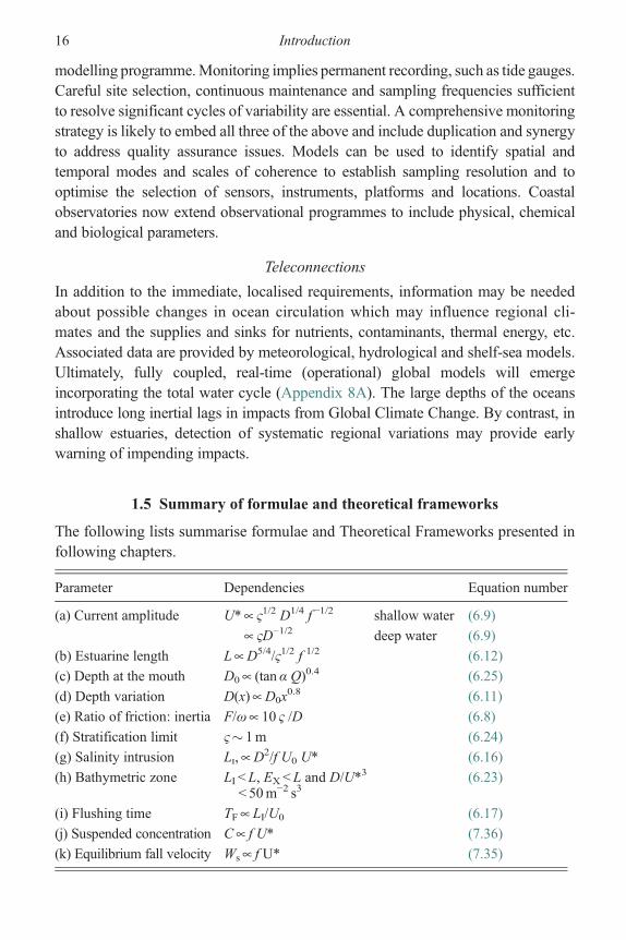
1.5 Summary of formulae and theoretical frameworks

The following lists summarise formulae and Theoretical Frameworks presented infollowing chapters.

Parameter Dependencies Equation number

(a) Current amplitude U*∝ ς1/2 D1/4 f −1/2 shallow water (6.9)

∝ ςD−1/2 deep water (6.9)

(b) Estuarine length L∝D5/4/ς1/2 f 1/2 (6.12)

(c) Depth at the mouth D0∝ (tan α Q)0.4 (6.25)

(d) Depth variation D(x)∝D0x0.8 (6.11)

(e) Ratio of friction: inertia F/ω∝ 10 ς /D (6.8)

(f) Stratification limit ς� 1m (6.24)

(g) Salinity intrusion Li,∝D2/f U0 U* (6.16)

(h) Bathymetric zone LI < L, EX < L and D/U*3

< 50m−2 s3(6.23)

(i) Flushing time TF∝ LI/U0 (6.17)

(j) Suspended concentration C∝ f U* (7.36)

(k) Equilibrium fall velocity Ws∝ f U* (7.35)

16 Introduction

ς is tidal elevation amplitude, f bed friction coefficient, Q river flow with currentspeed U0, tan α lateral inter-tidal slope, F linearised friction coefficient, ω tidalfrequency, Ex tidal excursion.Theoretical frameworks have been established to explain both amplitude and

phase variations of elevations and (cross-sectionally averaged) currents for theprimary tidal constituents. Qualitative descriptions of vertical current structurehave been derived for (i) oscillatory tidal components and (ii) residual componentsassociated with river flow, wind forcing and both well-mixed and fully stratifieddensity gradients. These dynamical results provide the basis for similar frameworksdescribing saline intrusion and sedimentation. Further applications of these theoriesfor synchronous estuaries enable the frameworks to be extended to illustrate con-ditions corresponding to stable bathymetry and sedimentary regimes.

Theoretical Framework Figure Question

(T1) Tidal response 2.5 Q2(T2) Current structure: (a) tidal 3.3 Q3

(b) riverine, wind and density gradient 4.4(T3) Saline mixing 4.13(T4) Sediment concentrations 5.6 Q5(T5) Bathymetry:

(a) Bathymetric zone 6.12 Q6(b) Stability 7.7 Q7(c) Lengths and depths 8.7(d) Ws, C, TF 7.11

Ws is the fall velocity for stable bathymetry, C is mean suspended sedimentconcentration and TF is flushing time. Q2 to Q8 refer to cardinal questions high-lighted in the Summary Sections of Chapters 2 to 8. Equation (4.44) addressesQ4 and Figs 7.9 and 7.10 and Table 8.4 address Q8. Figure 1.2 and Section 1.4summarise the issues concerned in Q1.

Appendix 1A

1A.1 Tide generation

Much of the theory presented here focuses on strongly tidal estuaries where the M2

constituent amplitudes are used as a basis for parameterising the linearised bed-friction coefficient, eddy viscosity and diffusivity together with related half-lives ofsediments in suspension. Figure 1A.1 shows tidal elevations in the Mersey, illustra-ting the predominance of the semi-diurnalM2 constituent. Here, we introduce a briefbackground to the generation of tides, illustrating their spectral and latitudinalvariations. For a rigorous, historical account of the development of tidal theory see

Appendix 1A 17

Cartwright (1999). For pictorial illustrations and simplified deductive steps for thefollowing theory see Dean (1966).Newton’s gravitational theory showed that the attractive force between bodies is

proportional to the product of their mass divided by the square of their distanceapart. This means that only the tidal effects of the Sun and the Moon need beconsidered. Mathematically, it is convenient to regard the Sun as rotating around a‘fixed’ Earth – enabling the same theory to be applied to the attraction from both theSun and the Moon.

1A.2 Non-rotating Earth

The attractive force on the Earth’s surface due to the Moon’s orbit can be separatedinto two components:

tangential3

2gM

E

a

d

� �3

sin 2θ (1A:1)

radial gM

E

a

d

� �3

ð1� 3 cos2 θÞ; (1A:2)

whereM/E is the ratio of the mass of the Moon to that of the Earth, i.e. 1/81, and a/dis the ratio of the radius of the Earth to their distance apart, i.e. 1/60. The longitude,

11.0

Gladstone dock1997

January 1997

10.0

9.0

8.0

7.0

6.0

5.0

Met

res

abov

e A

CD

4.0

3.0

2.0

1.0

0.0

–1.01 2 3 4 5 6 7 8 9 10 11 12 13 14 15 16 17 18 19 20 21 22 23 25 26 27 28 29 30 3124

Fig. 1A.1.Month-long recording of tidal heights at themouth of theMersey Estuary.

18 Introduction

θ, is measured relative to their alignment along the ecliptic plane of the Moon’sorbit. The radial force component is negligible compared with gravity, g.Integrating the tangential force, with the constant of integration determined from

satisfying mass conservation, indicates a surface displacement:

η ¼ a

4

M

E

a

d

� �3

ð3 cos 2θ þ 1Þ: (1A:3)

This corresponds to bulges on the sides of the Earth nearest and furthest from theMoon of about 35 cm, with depressions at the ‘poles’ of about 17 cm.

1A.3 Rotating Earth

Taking account of the Earth’s rotation, cos θ= cos� � cos λ, where � is latitude andλ the angular displacement and hence

η ¼ a

2

M

E

a

d

� �3

ð3 cos2 � cos2 λ� 1Þ: (1A:4)

Thus, we note the generation of two tides per day (semi-diurnal) with maximumamplitude at the equator �= 0 and zero at the poles �= 90°. The period of theprincipal solar semi-diurnal constituent, S2, is 12.00 h. The Moon rotates in 27.3days, extending the period of the principal lunar semi-diurnal constituent to 12.42 h.The ubiquitous spring–neap variations in tides follow from successive intervals ofcoincidence and opposition of the phases of M2 and S2. The two constituents are inphase when the Sun and the Moon are aligned with the Earth, i.e. both at ‘full moon’and ‘new moon’.

1A.4 Declination

The Moon’s orbit is inclined at about 5° to the equator; this introduces a dailyinequality in (1A.4), producing a principal lunar diurnal constituent, O1. The equiva-lent solar declination is 27.3°, producing the principal solar diurnal constituent P1alongside the principal lunar and solar constituent K1. The lunar declination variesover a period of 18.6 years changing the magnitude of the lunar constituents byup to ± 4%.

1A.5 Elliptic orbit

The Moon and the Sun’s orbits show slight ellipticity, changing the distance d in(1A.4). For the Moon, this introduces a lunar ellipse constituent N2, while for theSun constituents at annual, Sa, and semi-annual period, Ssa, are introduced.

Appendix 1A 19

1A.6 Relative magnitude of the Sun’s attraction

Although the ratio of masses, S/E= 3.3 × 105, overshadows that of M/E, this iscounterbalanced by the corresponding ratio of distances ds/dm� 390. Thus, therelative impact of Moon: Sun is given from (1A.4) as (S/M)/(ds/dm )3� 0.46.

1A.7 Equilibrium constituents

In consequence of the above, ‘equilibrium’magnitudes of the principal constituentsrelative to M2 are S2−0.46, N2−0.19, O1−0.42, P1−0.19 and K1−0.58.

1A.8 Tidal amphidromes

The integration of tidal potential over the spatial extent of the deep oceans meansthat ‘direct’ attraction in adjacent shelf seas can be neglected compared with thepropagation of energy from the oceans. In consequence, tides in enclosed seas andlakes tend to be minimal. In practice, the world’s oceans respond dynamically to theabove tidal forces. Responses in ocean basins and within shelf seas take the form ofamphidromic systems – as shown in Fig. 1A.2 (Flather, 1976) for theM2 constituentin the North Sea. The amplitudes of such systems are a maximum along their coastalboundaries, and the phases rotate (either clockwise or anti-clockwise) such that highwater on one side of the basin is balanced by low water on the other side. Whilethese surface displacements propagate around the system in a tidal period, the netebb or flood excursions of individual particles seldom exceeds 20 km.These co-oscillating systems can accumulate energy over a number of cycles (see

Section 2.5.4), resulting in spring tides occurring several days after new or full Moon.Basinmorphology can selectively amplify the amphidromes for different constituents.In general, the observed amplitudes of semi-diurnal constituents relative to diurnalare significantly larger than indicated from their equilibrium ratios shown above.

1A.9 Monthly, fortnightly and quarter-diurnal constituents

In shallow water and close to abrupt changes in bathymetry, tidal constituentsinteract (see Section 2.6). From the trignometric relationship

cosω1 � cosω2 ¼ 0:5 ðcosðω1 þ ω2Þ þ cosðω1 � ω2ÞÞ; ð1A:5Þa product of two constituents ω1 and ω2 results in constituents at their sum anddifference frequencies. Thus, terms involving products of M2 and S2 generateconstituents at the quarter-diurnal frequency MS4 and the fortnightly frequencyMSf. Similarly, M2 and N2 generate constituents at the quarter-diurnal frequencyMN4 and the monthly Mm.

20 Introduction

References

Cartwright, D.E., 1999. Tides: A Scientific History. Cambridge University Press,Cambridge.

Dean, R.G., 1966. Tides and harmonic analysis. In: Ippen, A.T. (ed.), Estuary and CoastlineHydrodynamics. McGraw-Hill, New York, pp. 197–230.

Fig. 1A.2. M2 tidal amphidromes in the north west European continental shelf.

References 21

Dyer, K.R., 1997. Estuaries: A Physical Introduction, 2nd ed. John Wiley, Hoboken, NJ.Flather, R.A., 1976. A tidal model of the north west European Continental Shelf,Memoires

Societe Royale des Sciences de Liege, Ser, 6 (10), 141–164.Lane, A. and Prandle, D., 2006. Random-walk particle modelling for estimating bathymetric

evolution of an estuary. Estuarine, Coastal and Shelf Science, 68 (1–2), 175–187.Liu, W.C., Chen, W.B., Kuo, J-T, and Wu, C., 2008. Numerical determination of residence

time and age in a partially mixed estuary using a three-dimensional hydrodynamicmodel. Continental Shelf Research, 28 (8), 1068–1088.

Prandle, D., 1982. The vertical structure of tidal currents and other oscillatory flows.Continental Shelf Research, 1, 191–207.

Prandle, D., 2004. How tides and river flows determine estuarine bathymetries. Progressin Oceanography, 61, 1–26.

Prandle, D., Lane, A., and Manning, A.J., 2005. Estuaries are not so unique. GeophysicalResearch Letters, 32 (23).

22 Introduction

2

Tidal dynamics

2.1 Introduction

Tidal propagation in estuaries can be accurately simulated using either numericalor hydraulic scale models. However, such models do not directly provide under-standing of the basic mechanisms or insight into the sensitivities of the controllingparameters. Thus, while terms representing friction and bathymetry appear expli-citly in (2.8) and (2.11), it is not immediately evident why tides are greatly amplifiedin certain estuaries yet quickly dissipated in others. The aim here is to deriveanalytical solutions, and thereby Theoretical Frameworks, to guide specific model-ling and monitoring studies and provide insight into and perspective on estuarineresponses generally.Much of the theory developed here assumes that tidal propagation in estuaries

can be represented by the shallow-water wave equations reduced to a 1D cross-sectionally averaged form. Section 2.2 describes the bases of this simplification.By further reducing these equations to a linear form, localised solutions are readilyobtained, these are examined in Section 2.3.It is shown in Section 2.4 that by introducing geometric expressions to approx-

imate estuarine bathymetry, whole-estuary responses can be determined. Tidalresponses in estuaries are shown for geometries approximated by (i) breadth anddepth variations of the form BL(X / λ)n and HL(X / λ)m, where X is the distance fromthe head of the estuary, i.e. the location of the upstream boundary condition at thelimit of tidal influence; (ii) breadth and depth varying exponentially and (iii) a‘synchronous’ estuary. Chapters 6 and 7 provide details of ‘synchronous estuaries’,their geometry is shown to correspond to (i) with m= n= 0.8. By expressing therelevant equations in dimensionless form, these analytical solutions are transposedinto Theoretical Frameworks, describing tidal elevations and currents over a widerange of estuarine conditions. Further details of current responses are described inChapter 3.

23

Where a single (M2) constituent predominates, this provides a robust basis forlinearisation of the friction term as outlined in Section 2.5. Tidal propagation inestuaries often involves large excursions over rapidly varying shallow topography.While first-order tidal propagation is relatively insensitive to small topographicchanges (Ianniello, 1979), Section 2.6 illustrates how the associated non-linearitiesresult in the generation of significant higher harmonic and residual components withpronounced spatial gradients.Finally, Section 2.7 indicates some of the peculiarities of surge–tide interactions.

2.2 Equations of motion

The equations of motion at any height Z (measured vertically upwards abovethe bed) along orthogonal horizontal axes, X and Y, may be written in Cartesianco-ordinates (neglecting vertical accelerations) as follows:Accelerations in X-direction:

@U

@tþU

@U

@Xþ V

@U

@Yþ g

@&

@X� ΩV ¼ @

@ZE@U

@Z(2:1)

Accelerations in Y-direction:

@V

@tþU

@V

@XþV

@V

@Yþ g

@&

@YþΩU ¼ @

@ZE@V

@Z(2:2)

Continuity:

@U

@Xþ @V

@Yþ @W

@Z¼ 0; (2:3)

whereU, VandWare velocities along X, Yand Z, ς is surface elevation,Ω= 2ω sin φis the Coriolis parameter representing the influence of the earth’s rotation (ω=2π/24 h), φ is latitude and E is a vertical eddy viscosity coefficient. Forcing due towind and variations in density or atmospheric pressure is omitted in (2.1) and (2.2).For many applications, it is convenient to vertically integrate between the bed and

the surface. The depth-averaged equations retain the same form except that

(1) the non-linear convective terms U (∂U/∂X) +V (∂U/∂Y) in (2.1) and U (∂V/∂X) +V (∂V/∂Y) in (2.2) are multiplied by coefficients dependent on the vertical structure ofU and V;these coefficients are often assumed to equal 1 for simplicity;

(2) with zero surface stress, the vertical viscosity terms are replaced by bed stress termsτx/ρD and τy/ρD, assumed to be proportional to the respective components of bedvelocity squared, i.e.

τx ¼ �ρfUðU2 þ V2Þ1=2; τy ¼ �ρfVðU2 þ V2Þ1=2; (2:4)

where ρ is water density and f is the bed stress coefficient (≈0.0025)

24 Tidal dynamics

(3) the kinematic boundary condition at the surface and bed is:

Ws ¼ @&

@tþU

@&

@Xþ V

@&

@Y

and

W0 ¼ �U@D

@X� V

@D

@Y: (2:5)

These yield a depth-integrated continuity equation:

Dþ &ð Þ @&@t

þ @

@XU Dþ &ð Þ þ @

@YV Dþ &ð Þ ¼ 0 (2:6)

Ianniello (1977) indicates that transverse velocities can be neglected if the KelvinNumber ΩB/(gD)1/2≪ 1 and the horizontal aspect ratio B2ω2/(gD)≪ 1 (B breadth,ω = 2π/P, P tidal period). Thence adopting X axially, by integrating acrossboth breadth and depth, (2.1) may be rewritten in cross-sectionally averagedparameters as

@U

@tþU

@U

@Xþ g

@&

@Xþ f

UjUjDþ &ð Þ ¼ 0 (2:7)

and the continuity equation (2.6) as

B Dþ &ð Þ @&@t

þ @

@XBUA ¼ 0; (2:8)

where A is the cross-sectional area.Although lateral velocities may be restricted in estuaries, the transverse Coriolis

term ΩU, in (2.2), must be balanced, generally by a lateral surface gradient. Thisgradient produces an elevation phase advance on the right-hand side (lookinglandwards in the northern hemisphere) of the order of BΩ/(2(gD)1/2) radians(Larouche et al., 1987).The relative magnitudes of the terms in (2.7) for a predominant tidal frequency ω

are approximately

ωU� :2πU�2

λ:2π&�gλ

:fU�2

D; (2:9)

where λ is the wavelength over which both U and ς vary. Assuming λ= (gD)½P, therelative magnitudes of the first two terms are

ðgDÞ1=2 : U�: (2:10)

Thus, the ratio of the magnitudes of the convective term and the temporal accelera-tion term is equal to the Froude number for the flow. This is generally small, and

2.2 Equations of motion 25

hence for first-order tidal simulation, the convective terms can be neglected. Therelative magnitude of the friction term to the temporal acceleration term for thesemi-diurnal frequency and f = 0.0025 is approximately 20 U*/D s−1, i.e. predomi-nant in fast-flowing shallow estuaries (see Section 2.3.2). In such estuaries, thefrictional force greatly exceeds the acceleration (inertial) term over most of the tidalcycle and wave propagation is diffusive in character (LeBlond, 1978).

2.3 Tidal response – localised

It is shown in Section 2.4.2 that combining the two equations, (2.7) and (2.8), producesan expression for tidal response along an estuary similar to the spectral response fora linearly damped, single-degree-of-freedom oscillatory system executing ‘simpleharmonic motion’. Thus, we expect harmonic solutions with axial variations in tidalamplitudes and phases described by Bessel functions, as illustrated in Section 2.4.1.

2.3.1 Linearised solution

Neglecting the convective term and linearising the friction term in (2.7) (seeSection 2.5 for details of this linearisation) yields

@U

@tþ g

@&

@Xþ FU ¼ 0: (2:11)

It is readily shown that in a prismatic channel of infinite length and zero friction,(2.8) and (2.11) indicate a wave celerity, c= (gD)1/2 and U* = ς(g/D)1/2 (Lamb,1932). Maximum amplification then occurs for quarter-wave resonance at lengthL= 0.25λ= 0.25 P (gD)1/2. It is shown in Section 2.4.1 that even in damped,funnel-shaped estuaries, maximum amplification often occurs for values of L closeto this value.Introducing a surface gradient for a predominant constituent in the form

@&

@X¼ &�x cosωt (2:12)

from (2.11), we obtain

U� ¼ �g&�xðF2 þ ω2Þ ðF cosωtþ ω sinωtÞ: (2:13)

Thus, for a frictionally dominated system F≫ω,

U� ¼ �g&�x=F cosωt; (2:14)

while for a frictionless system F≪ω,

26 Tidal dynamics

U� ¼ �g&�x =ω sinωt: (2:15)

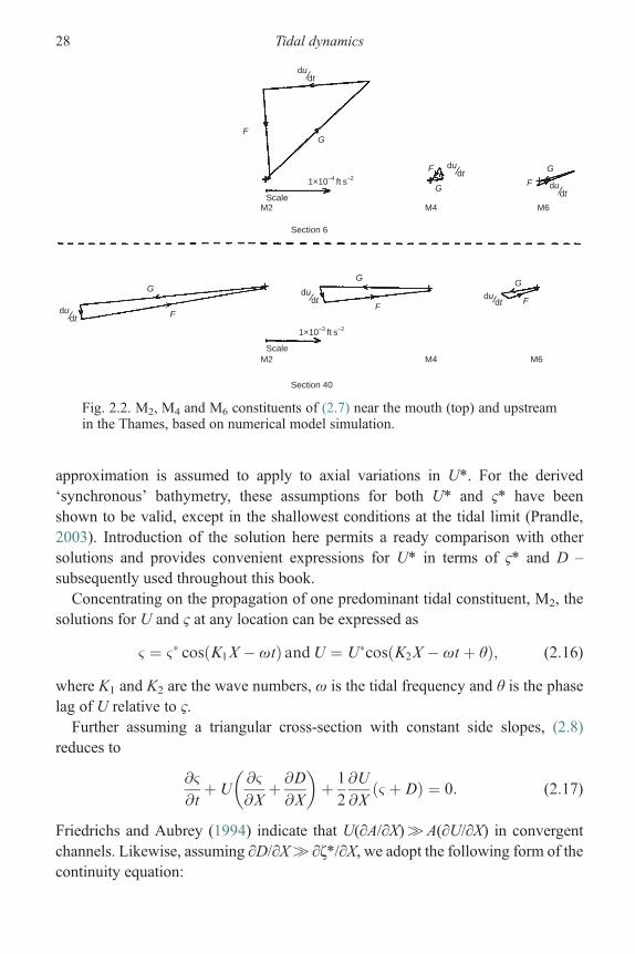
Figure 2.1 indicates the solution of (2.13) for prescribed values of surface gradientup to 0.00025 g and depths of 4, 16 and 64m. For the deepest case, the solutionapproximates (2.15) while the shallowest case approximates (2.14).Figure 2.2 shows the magnitude of the terms in (2.7) at two positions in the Thames

for the predominant M2 constituent and the related higher harmonics M4 and M6, ascalculated in a numerical model simulation (Prandle, 1980). For M2, the inertial andfrictional terms are orthogonal in phase and balance the surface gradient term.By contrast, for M4 and M6, the spatial gradient term is a consequence of ratherthan a driving force for currents (see Section 2.6) and hence different relationshipsapply.

2.3.2 Synchronous estuary solution

A ‘synchronous estuary’ is one where surface gradients associated with axialamplitude variations in ς* are significantly less than those associated with corre-sponding phase variations. In deriving solutions to (2.8) and (2.11), a similar

2.0

1.5

1.0

0.5

Veloc

ity a

mpl

itude

(m

s–1

)

0.00 5.0 × 10–5 1.0 × 10–4

Surface gradient amplitude ( × g)

1.5 × 10–4 2.0 × 10–4 2.5 × 10–4

No friction

Depth = 4 m

No inertia

D = 64 m

D = 16 m

Fig. 2.1. M2 tidal current amplitude as a function of surface gradient. Continuouslines show solution (2.13) for D = 4, 16 and 64 m. Dashed lines show solution(2.14) for D= 4 m and (2.15) for D = 64 m.

2.3 Tidal response – localised 27

approximation is assumed to apply to axial variations in U*. For the derived‘synchronous’ bathymetry, these assumptions for both U* and ς* have beenshown to be valid, except in the shallowest conditions at the tidal limit (Prandle,2003). Introduction of the solution here permits a ready comparison with othersolutions and provides convenient expressions for U* in terms of ς* and D –

subsequently used throughout this book.Concentrating on the propagation of one predominant tidal constituent, M2, the

solutions for U and ς at any location can be expressed as

& ¼ &� cosðK1X� ωtÞ andU ¼ U�cosðK2X� ωtþ θÞ; (2:16)

where K1 and K2 are the wave numbers, ω is the tidal frequency and θ is the phaselag of U relative to ς.Further assuming a triangular cross-section with constant side slopes, (2.8)

reduces to

@&

@tþU

@&

@Xþ @D

@X

� �þ 1

2

@U

@X& þDð Þ ¼ 0: (2:17)

Friedrichs and Aubrey (1994) indicate that U(∂A/∂X)≫A(∂U/∂X) in convergentchannels. Likewise, assuming ∂D/∂X≫ ∂ζ*/∂X, we adopt the following form of thecontinuity equation:

dudt

F

F

F

FF

F

G

G

G

GG

G

Scale

Scale

M2

Section 6

Section 40

1×10 –4 ft s–2

1×10 –3 ft s–2

M4 M6

M2 M4 M6

dudt

dudt du

dt

dudt

dudt

Fig. 2.2. M2, M4 and M6 constituents of (2.7) near the mouth (top) and upstreamin the Thames, based on numerical model simulation.

28 Tidal dynamics

@&

@tþU

@D

@XþD

2

@U

@X¼ 0: (2:18)

Substituting solution (2.16) into Eqs (2.11) and (2.18), four equations (pertaining atany specific location along an estuary) representing components of cosωt and sinωtare obtained. By specifying the synchronous estuary condition that the spatialgradient in tidal elevation amplitude is zero, the condition K1 =K2 = k is derived,i.e. identical wave numbers for axial propagation of ς and U. Then, the followingsolutions for the amplitude, U*, and phase, θ, of tidal current together with bedslope, SL= ∂D/∂X, are obtained:

tan θ ¼ � F

ω¼ SL

0:5Dk; U� ¼ &�g

k

ðω2 þ F2Þ1=2; k ¼ ω

Dg=2ð Þ1=2: (2:19)

Results

The above solutions are consistent with (2.13), the celerity 0.5 (gD)½ follows fromthe assumption of a triangular cross section. Chapter 6 illustrates how these explicitsolutions for U*, θ and SL enable other related parameters, such as estuarine length,to be determined, yielding a range of Theoretical Frameworks in terms of theparameters D and ς*. The parameter ranges selected are ς* (0–4m) and D (0–40m),representing all but the deepest of estuaries.

Current amplitudes U

Figure 2.3 shows the solution (2.19) with current amplitudes extending to 1.5m s−1

(Prandle, 2004).The contours show that maximum values ofU* occur at approximatelyD=5+10 ς* (m); however, these are not pronounced maxima. This figure explainswhy observed values of U* are so often in the range 0.5–1.0 m s−1 despite largevariations in ς* over the spring–neap cycle and the wide range of estuarine depths.

Role of bed friction

Friedrichs and Aubrey (1994) showed the predominance of the friction term instrongly convergent channels, irrespective of depth. Figure 2.4 shows the ratio offriction: inertia, F/ω, from (2.19) (Prandle, 2004). F/ω is approximately equal tounity for ς* =D/10. For ς*≪D/10, currents are insensitive to friction, while forς*≫D/10, tidal dynamics become frictionally dominated and currents decrease bya factor of two as the friction coefficient increases over its typical range from 0.001to 0.004. Prandle (2003) provides a detailed analysis of the sensitivities to thefriction parameter. From (2.19), for F � ω; U�/ &�1=2D1=4f�1=2while forF � ω;U�/ &�D�1=2:

2.3 Tidal response – localised 29

From (2.19), F/ω= 0.1 corresponds to a phase difference between tidal elevationand currents of θ=−6°. Similarly, F/ω= 0.5 corresponds to θ=−27°, 1.0 to −45°,2 to −63°, 5 to −77° and 10 to −84°. These values of θ emphasise how the tidal wavepropagation changes from ‘progressive’ in deeper water closer to the mouth to‘standing’ in shallower water at the head.

Fig. 2.4. Ratio F:ω of the friction term F to the inertial term as a f (D, ς*) (2.19).

Fig. 2.3. Tidal Current amplitude, U* (m s−1), as a f (D, ς*) (2.19).

30 Tidal dynamics

Rate of funnelling in a synchronous estuary

By integration of the solution for bed slope, SL, in (2.19), it can be shown that thesynchronous solution corresponds to depths and breadths proportional to X 0.8, i.e.m= n= 0.8 in (2.20) and (2.21). Comparing the localised synchronous solutionsto the whole-estuary response in Section 2.4.1, this synchronous geometry corre-sponds to ν= 1.5. From Fig. 2.5, this is close to the centre of the range of geometriesencountered (Prandle, 2004). Moreover, the estuarine lengths determined for syn-chronous estuaries, incorporated in Fig. 2.5, range from a small fraction up to closeto that for ‘quarter-wavelength’ (first node), resonance at the M2 frequency.

2.4 Tidal response – whole estuary

This section is concerned with the first-order response of whole estuaries to tidalforcing. The aim is to construct simplified analytical frameworks that answer suchbasic questions as to why (i) tides are large in some estuaries, (ii) semi-diurnalconstituents are sometimes amplified while diurnals are often damped and (iii) someestuaries are sensitive to small changes in bed friction, length or depth. Simplified

Fig. 2.5. Tidal elevation responses (2.24) for s− 2π. ν represents the degree ofbathymetric funnelling and y distance from the mouth, y= 0. Dashed contoursindicate relative amplitudes, continuous contours relative phases. Vertical line atν = 1.5 shows typical lengths of synchronous estuaries (see Chapter 6). Lengths,y (for M2) and shapes, ν, for estuaries (A)–(I) shown in Table 2.1.

2.4 Tidal response – whole estuary 31

analytical solutions to (2.8) and (2.11) have been presented by Taylor (1921),Dorrestein (1961) and Hunt (1964). Here we discuss more generalised solutionsfor (i) breadth and depth varying with powers of distance X (Prandle and Rahman,1980, subsequently Prandle and Rahman, 1980) and (ii) breadth and depth varyingexponentially with X (Prandle, 1985). Since these responses are based on thelinearised equations, they are generally applicable to estuaries with a predominanttidal constituent.Taylor’s frictionless solution for an estuary with linearly varying depth and breadth

represents a special case of (i). Hunt’s analytical solutions for estuaries with expo-nentially increasing breadth and constant depth are presented in Section 2.4.2.

2.4.1 Breadth and depth varying with powers of distance X(Prandle and Rahman, 1980)

Breadth and depth are assumed to vary by

BðXÞ ¼ BLX

λ

� �n

(2:20)

and

HðXÞ ¼ HL

X

λ

� �m

(2:21)

with Xmeasured from the head of the estuary. To convert to a dimensionless format,we adopt λ as a unit of horizontal dimension, HL as a unit of vertical dimension andP, the tidal period, as a unit of time, with

λ ¼ ðgHLÞ1=2P (2:22)

corresponding to the tidal wavelength for HL constant. Dimensionless parametersare introduced as follows:

x ¼ X=λ; t ¼ T=P; h ¼ H=HL; b ¼ B=λ; u ¼ UP=λ; frictional parameter s ¼ FP:

(2:23)

Prandle and Rahman (1980) showed that the substitution of (2.20) and (2.21) into(2.8) and (2.11) yields the following solution for tidal elevation ς at any location x, atany time t, for any tidal period P:

& ¼ &�ky

kyM

� �1�νJν�1ðkyÞJν�1ðkyMÞ e

i2πt; (2:24)

where ς* ei2πt is the tidal elevation at the mouth xM and

32 Tidal dynamics

ν ¼ nþ 1

2�m; k ¼ 1� is

2π

� �1=2

y ¼ 4π2�m

x2�m2 (2:25)

and Jν − 1, is a Bessel function of the first kind and of order v− 1.The solution (2.24) is illustrated in diagrammatic form in Fig. 2.5 for the case of

s= 2π, i.e. F=ω. Prandle and Rahman (1980) show the corresponding solutions fors= 0.2π. Away from the resonant conditions illustrated in Fig. 2.6, the responses forthe two frictional coefficients are essentially similar, with reduced amplitudes andenhanced phase differences for the larger friction coefficient. This figure constitutesa general response diagram showing the variation in amplitude and phase of tidalelevations along the length of an estuary. For the M2 semi-diurnal constituent, thepositions indicated (A)–(I) designate the mouths of the major estuaries listed inTable 2.1.Confidence in the validity of this approach was shown by comparing results for

M2 elevation response for the ten major estuaries listed in Table 2.1. In all of these

s = 0.2π

s = 2π

Fig. 2.6. Frequency response for tidal elevations in the Bay of Fundy (2.24), withs= 0.2π and 2π. Vertical scale shows amplification at the head relative to values atthe shelf edge encircled dots represent observed data.

2.4 Tidal response – whole estuary 33

estuaries, good agreement was found using s= 2π, except for the Bay of Fundy (G),where with depths exceeding 200m better agreement was found for s= 0.2π.Given the funnelling factor v and length yM for a particular estuary, the variation

in amplitude and phase in the estuary can be read along the corresponding verticalline. Moreover, the value of yM is inversely proportional to the tidal period P, thusdoubling P halves yM. Using this relationship, Fig. 2.6 illustrates the spectralresponse for the Bay of Fundy. Strictly, some adjustment is necessary to reflectthe 50% increase in the friction factor appropriate to constituents other than thepredominant M2 – as described in Section 2.5. Similar response diagrams to Fig. 2.5can be constructed for amplitudes and phases of tidal currents.In summary, Fig. 2.5 constitutes a general tidal response diagram indicating

amplitudes and phases (relative to the mouth) at all positions, for all tidal periods,for all estuaries which reasonably correspond to (2.11) and (2.12). This responsediagram explains a number of features commonly encountered:

(1) The quarter-wavelength resonance or primary mode found in sufficiently long estuariesis indicated by the thick line through the amplitude nodes.

(2) For a diurnal tidal constituent, the yMvalues (A)–(I) are halved; hence, we expect relativelysmall amplification of such constituents. For MSf, a 14-day constituent, the reduction inthe yM values would indicate little amplification or phase difference along any estuary.

(3) For quarter-diurnals or other higher harmonics, in relative terms we expect highamplification, large phase differences and one or more nodal positions. However, it isimportant to distinguish between the response to external forcing represented by thepresent analysis versus the internal generation of higher harmonics by non-linear pro-cesses within an estuary discussed in Section 2.6 and illustrated in Fig. 2.2.

Table 2.1 Geometrical parameters for ten estuaries shown in Fig. 2.5

HM (m) L (km) n m ν y0 H0 (m) α β α+ 2β

A Fraser 44 135 −0.7 0.7 0.2 3.0 2.3 −2.8 2.8 2.8B Rotterdam Waterway 13 99 0 0 0.5 1.2 13.0 0 0 0C Hudson 17 248 0.7 0.4 1.1 4.2 4.8 2.2 1.3 4.8D Potomac 13 184 1.0 0.4 1.3 3.7 3.5 3.6 1.4 6.4E Delaware 5 214 2.1 0.3 1.8 5.3 2.3 5.3 0.8 6.9F Miramichi 7.0 55 2.7 0 1.9 0.9 7.0 46.6 0 46.6G Bay Fundy 2000 635 1.5 1.0 2.4 3.8 21.4 3.9 2.6 9.1H Thames 80 95 2.3 0.7 2.5 1.77 2.7 14.1 4.3 22.7I Bristol Channel 5000 623 1.7 1.2 3.4 5.20 12.5 3.4 2.4 8.2J St. Lawrence 300 418 1.5 1.9 19.5 1 1.3 1.6 4.5

Notes: HM depth at mouth, H0 depth at head, L and y0 estuarine lengths (from (2.25))n, m, ν, α and β bathymetric parameters.Source: Prandle and Rahman, 1980; Prandle, 1985

34 Tidal dynamics

Quarter-wavelength resonance

The position of the first nodal line in Fig. 2.5, corresponding to maximum ampli-fication in estuaries with varying degrees of funneling, is approximated by

y ¼ 1:25þ 0:75ν; i:e: x ¼ 3n� 5mþ 13

16π

� �ð2=2�mÞ: (2:26)

The ratio of resonant lengths, (2.26), as a fraction of that for a prismatic channel,(2.22), is x(1−m/2)/0.25.Table 2.2 shows this ratio, for the typical ranges of 0 < n< 2.5 and 0 <m< 1,

including the value m= n= 0.8 corresponding to the solution for a synchronousestuary (Section 2.3.2). These results indicate that upstream reductions in depthsdecrease resonant lengths while breadth convergence has the opposite effect, empha-sising the complexity of tidal response in funnel-shaped estuaries.

2.4.2 Depth and breadth varying exponentially(Hunt, 1964; Prandle, 1985)

Assuming a breadth and depth variation:

BðXÞ ¼ B0 expðnXÞHðXÞ ¼ H0 expðmXÞ; (2:27)

where B0 and H0 are the respective values at the head X= 0, we convert todimensionless units based on the tidal period P as the unit of time. H0 as the verticaldimension and λ the horizontal dimension given by

λ ¼ ðgH0Þ1=2P: (2:28)

Thus, we obtain transformed dimensionless variables: x =X/λ, t = T/P, z = Z/H0,b=B/λ, h =H/H0, u=U(P/λ), s=FP and

bðxÞ ¼ b0 expðαxÞ (2:29)

and

Table 2.2 Resonant lengths for funnel-shaped estuaries, B∝Xn

and D∝Xm, (2.26), as a fraction of the prismatic value (2.22)

m =n 0 0.8 1.0

0 1.04 0.74 0.570.8 1.23 0.91 0.832.5 1.64 1.33 1.26

2.4 Tidal response – whole estuary 35

hðxÞ ¼ expðβxÞ; (2:30)

where α= nλ and β=mλ.Substituting (2.29) and (2.30) into (2.8) and (2.11), these equations may be

rearranged to form separate expressions for either ς or u. The time derivatives inthese expressions may be eliminated by considering amplitudes pertaining to asingle period P, thus

& ¼ &� expði2πtÞ and u ¼ u� expði2πtÞ: (2:31)

The expressions for the tidal amplitudes ς and u are then as follows:

@2

@x2&� þ ðαþ βÞ @&

�

@xþ ð4π2 � 2πisÞ &�

expðβxÞ ¼ 0 (2:32)

@2u�

@x2þ ðαþ 2βÞ @u

�

@xþ βðαþ βÞ þ ð4π2 � 2πisÞ

expðβxÞ� �

u� ¼ 0: (2:33)

By introducing appropriate transformations, the middle terms (involving the singlederivative in x in (2.32) and (2.33)) may be eliminated. The resulting equationsmay then be solved analytically (Gill, 1982, Section 8.12). Such solutions have beenexamined by Xiu (1983); however, their complexity obscures direct understanding.In the following section, we consider simpler analytical solutions relating to certainspecial cases alongside a numerical solution to illustrate the nature of the responses.

(1) Solutions for constant depth, β = 0: Hunt (1964) showed that for this case the solutionsto (2.32) and (2.33) are

& ¼ &�0 exp�α x

2

� �coshωxþ α

2ωsinhωx

� �(2:34)

u ¼ �&�0 exp�α x

2

� � 2πiα

sinhωx; (2:35)

where ω=ω1 + i ω2, ω12−ω2

2 = α2/4 − 4π2, ω1·ω2 = πs and ς*0 is the elevation ampli-tude at the head, x= 0.

(2) Solutions for constant depth, β = 0 and zero friction: For this case, (2.32) and (2.33)described the free vibrations of a damped simple harmonic oscillator. Using thisanalogy, for α < 4π the system is under-damped, α = 4π represents critical dampingwhile α > 4π is over-damped.

For α>4π, the solutions retain the form shown in (2.34) and (2.35)withω12 =α2/4− 4π2

and ω2 = 0.For α < 4π, the solutions simplify to

&� ¼ &�0 exp�αx2

� �cosω2xþ α

2ω2

sinω2x

� �(2:36)

36 Tidal dynamics

u� ¼ �&�0 exp�αx2

� � 2πiω2

sinω2x (2:37)

with ω22 = −α2/4 + 4π2.

For α = 4π, the following specific solutions apply

&� ¼ &�0 expð�2πxÞð1þ 2πxÞ (2:38)

u� ¼ &�0 expð�2πxÞ2πix: (2:39)

(3) Numerical solution for both depth and breadth varying exponentially and friction.The general response diagram is shown in Fig. 2.7 (Prandle, 1985), for s= 2π, the

orthogonal axes refer to the parameters α and β. The contours show the amplificationbetween the amplitude of the tidal elevation at the head of the estuary relative to thevalue at the first nodal position. However, for estuaries with values of α + 2β> 10, nonodal position occurs and in this case the amplification shown is relative to the value forx= 1 where the latter value closely approximates the asymptote at x=∝. This demarca-tion in the response of estuaries at α+ 2β= 10 was not evident in the solution in Section2.4.1. The symbols (A)–(J) again indicate the amplification for all ten major estuaries,listed in Table 2.1, between the head and the first nodal position or x= 1 (not the mouth)for the semi-diurnal constituent M2.

Fig. 2.7. Tidal elevation amplification as a function of α and β, s= 2π (2.32).

2.4 Tidal response – whole estuary 37

To determine the maximum response for other tidal constituents from Fig. 2.7, wenote that the values for α and β are directly proportional to period; thus, for diurnalconstituents α and β are doubled while for quarter-diurnal constituents α and β arehalved. In consequence, we may deduce the following conclusions from the generalresponse diagram, Fig. 2.7 and the analytical solutions in Section 2.4.2.

(a) The response of any estuary may be likened to the free vibrations of a damped simpleharmonic oscillator. Estuaries of type I with α + 2β< 10 are under-damped and elevationamplitudes vary in an oscillatory manner along the x-axis. Estuaries of type II withα + 2β ~ 10 are critically damped and produce maximum amplification. Estuaries of typeIII with α + 2β≫ 10 are over-damped and elevations increase monotonically towardsthe head with little amplification and little sensitivity to frictional effects. The value of10 is approximate, the corresponding value of 4π was determined for the zero-frictioncase in Section 2.4.2(2).

(b) The Bristol Channel (I) and Bay of Fundy (G) both lie close to the demarcation line,α + 2β� 10, in Fig. 2.7, explaining the sensitive ‘near-resonant’ nature of the responseof these two systems. These responses are a consequence of their particular values of αand β (for the M2 constituent) and not simply due to their resonant lengths as generallyassumed.

2.5 Linearisation of the quadratic friction term

2.5.1 Single constituent

The preceding analyses required the quadratic friction term f1U|U| to be approxi-mated by a linear term f2U. For a single constituent U=U1cos ωt, equating energydissipation, proportional to U3, over a tidal cycle requires f2 = (8/3π) f1U1.

2.5.2 Two constituents

Proudman (1923) and Jeffreys (1970) showed that where two tidal stream consti-tuents U1 cos ωt and U1

0 cos ω0t coincide, the friction term is given by

f1ðU1 cosωtþU01 cosω

0 tÞ U1 cosωtþU01 cosω

0t�� ��: (2:40)

Then, for small values ofU 01, the linearised friction component Fω at the frequency

of ω is given, to a first approximation, by

Fω ¼ 8 f13π

� �U2

1 cosωt ¼ f2 U1 cosωt (2:41)

while the component at the frequency ω0 is

Fω0 ¼ 4

π

� �f1 U1 U

01 cosω

0 t ¼ 3

2

� �f2 U0

1 cosω0t: (2:42)

38 Tidal dynamics

In the case of a small residual current U0 coincident with a large tidal streamU1 cosωt, Bowden (1953) showed that, with U1≫U0, the linear friction termassociated with the residual current is given by

F0 ¼ 4

π

� �f1U1 U0 ¼ 3

2

� �f2 U0: (2:43)

Hence, (2.41), (2,42) and (2.43) show that to account for the interaction with apredominant M2 constituent in a linearised model, when simulating separately anyother tidal constituent or a residual flow, the linearised frictional coefficients fR mustbe computed according to

fR ¼ 3

2

� �f2: (2:44)

The magnitude of the tidal streams due to M2 in mid-latitudes is typically of ordertwo or three times the magnitude of the next largest constituent, S2. Hence, it isreasonable, in simulating M2 alone, to neglect the frictional interaction due toother constituents and use (2.41). However, in simulating any other tidal consti-tuent, it is appropriate to linearise the frictional term by reference to the tidalvelocities associated with M2 by using (2.44). Hence, relative to other terms in themomentum equation, the linearised friction coefficient for other constituents, ω0, isa factor 1.5 UM2

=Uω0 larger. In the north west shelf seas, S2 amplitudes aretypically 0.33 of M2, whereas the ratio of their ‘equilibrium’ potentials is 0.46,(Appendix 1A). Thus, increasing the linearised S2 friction factor by a factor of4.5 (relative to that for propagation of M2) appears to reduce S2 amplitudes byabout 1/3.Garrett (1972), Hunter (1975) and Saunders (1977) discuss the extension of the

above results for flow in two dimensions.

2.5.3 Triangular cross section

For the synchronous solution, Section 2.3.2, the component of f (U|U|/D) at thepredominant tidal frequency M2 was approximated by

8

3π25

16fjU�jUD

¼ FU; (2:45)

i.e. F= 1.33 f U*/D, where 8/3π derives from the linearisation of the quadraticvelocity term described above. The factor 25/16 is included to weight the frictionalterm close to the largest flow which occurs in the deepest water where, from (2.19)with F≫ω, the maximum velocity is 5/4 of the cross-sectional mean.

2.5 Linearisation of the quadratic friction term 39

2.5.4 Q factor (Garrett and Munk, 1971)

Analogies between the propagation of tides in a channel and the transmission ofelectrical energy in an AC circuit were made by Van Veen (1947) and Prandle(1980). The analogy links tidal elevations to voltage, tidal streams to current, bedfriction to resistance and, somewhat less directly, inertial effects to inductance andsurface area to capacitance. The analogy is dependent on the assumption that tidalpropagation is sensibly linear and lightly damped. Evidence that tidal propagation isessentially linear in oceans and shelf seas follows from the accuracy of tidal predic-tion techniques, i.e. the harmonic method and, in particular, the response method(Munk and Cartwright, 1966).The relative influence of the friction term in (2.11) was discussed in Section 2.3.

Using the above analogy with an AC electrical circuit, a succinct quantificationof frictional influence is provided by the quantity Q, known as the quality factor(Q factor). An oscillating system dissipates 2π/Q of its energy each cycle. Forsystems near resonance,

Q ¼ ωo

ω2 � ω1

(2:46)

is a measure of the sharpness of resonance, based on the ratio of the natural frequency,ω0, to the frequency difference between points on the response curve, ω2 and ω1,corresponding to half the power dissipation of that at the natural frequency.Godin (1988) showed that for (2.11), the Q factor of tidal basins is given by

Q=ω/F. Thus, the value of s=FP= 2π used in reproducing the responses ofestuaries in Section 2.4 is equivalent to Q= 1 and emphasises that most estuariesare highly dissipative. Conversely, in Fundy, for which s= 0.2π, Q= 10, indicatinga more sharply resonant system. These estuarine values forQmay be compared withthe value of Q ≈ 17 computed for the North Atlantic by Garrett and Greenberg(1977).In ‘spinning-up’ a numerical simulation of tidal propagation starting from

still-water conditions, it similarly follows from (2.11) that cyclical convergence oftidal amplitudes is approached asymptotically at a rate (1– exp(−Ft)).

2.6 Higher harmonics and residuals

The above theories provide robust descriptions of the first-order estuarine responsesfor the primary tidal constituents. However, subsequent chapters emphasise thelonger-term importance to both mixing processes and sediment dynamics of see-mingly ‘second-order’ effects, namely higher-order and residual tides alongsidevertical, lateral and high-frequency variability in currents and salinity. Whilethe first-order effects can be accurately modelled, numerical simulation of these

40 Tidal dynamics

‘second-order’ effects requires increasingly fine resolution in both space and time.Thus, ironically, despite the rapid growth in computer power since the first simple,but successful, numerical tidal models, limitations in computing power remain anobstacle to progress. Here, we explain how these higher harmonic and residualterms are generated.

2.6.1 Trigonometry

Although the tidal forcing at the mouth of an estuary is primarily at the semi-diurnal or diurnal frequencies, the non-linear terms in (2.1) to (2.5) almost alwaysproduce significant higher harmonics in shallow water (Aubrey and Speer, 1985).This process can be understood from simple trigonometry in which

U�1 cosðω1tÞ � U�

2 cosðω2tÞ ¼ U�1U

�2

2cosðω1 � ω2Þtþ cosðω1 þ ω2Þtð Þ:

(2:47)

Thus, terms involving a product of the predominant M2 constituent generate bothM4 and Z0 constituents. Similarly, whenever two large constituents are present (e.g.M2 and S2), the same mechanisms generate constituents at their sum frequency(ω1 +ω2) =ωMS4

and the difference frequency (ω2 –ω1) =ωMSf, i.e. quarter-diurnal

and fortnightly periods, or for (M2 +N2), quarter-diurnal and monthly periods.These residuals and higher harmonics manifest themselves via features such asasymmetry between ebb and flood flows (particularly M4), occasional double highwaters and tidal pumping (in which an estuary exchanges water over a neap–springcycle complicating mass-balance calculations based on observations made over asingle semi-diurnal period). In formulating models to examine these residual andhigher harmonics, it should be recognised that the scaling arguments used to derive(2.11), based on the predominant constituent, may be invalidated. In particular, forhigher harmonics, the wavelength λ associated with the variability ofU and ςmay bedetermined by bathymetry (Zimmerman, 1978).

2.6.2 Non-linear terms in the tidal equations

A convenient device to illustrate the nature of these non-linearities is to rewrite (2.1)and (2.6) in terms of mass transports. These equations then take the following form(Prandle, 1978):

@

@tQx þ @

@X

Q2x

Hþ @

@X

QxQy

HþHg

@&

@Xþ g

f QxðQ2x þQ2

yÞ1=2H2

� ΩQy ¼ 0

(2:48)

2.6 Higher harmonics and residuals 41

@

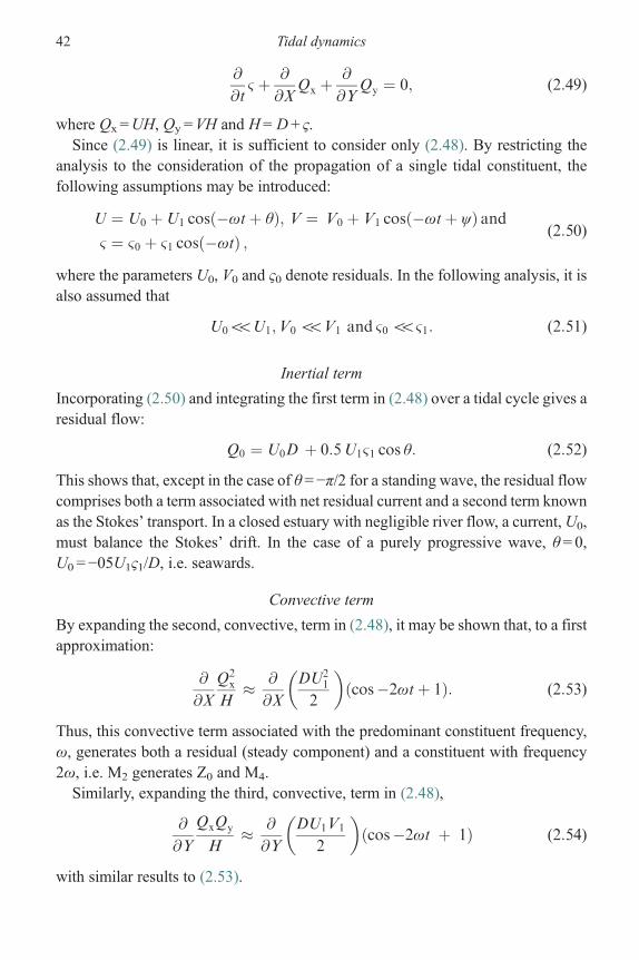
@t& þ @

@XQx þ

@

@YQy ¼ 0; (2:49)

where Qx =UH, Qy =VH and H=D+ ς.Since (2.49) is linear, it is sufficient to consider only (2.48). By restricting the

analysis to the consideration of the propagation of a single tidal constituent, thefollowing assumptions may be introduced:

U ¼ U0 þU1 cosð�ωtþ θÞ; V ¼ V0 þ V1 cosð�ωtþ ψÞ and& ¼ &0 þ &1 cosð�ωtÞ ; (2:50)

where the parameters U0, V0 and ς0 denote residuals. In the following analysis, it isalso assumed that

U055U1;V0 55V1 and &0 55&1: (2:51)

Inertial term

Incorporating (2.50) and integrating the first term in (2.48) over a tidal cycle gives aresidual flow:

Q0 ¼ U0D þ 0:5U1&1 cos θ: (2:52)

This shows that, except in the case of θ=−π/2 for a standing wave, the residual flowcomprises both a term associated with net residual current and a second term knownas the Stokes’ transport. In a closed estuary with negligible river flow, a current,U0,must balance the Stokes’ drift. In the case of a purely progressive wave, θ= 0,U0 =−05U1ς1/D, i.e. seawards.

Convective term

By expanding the second, convective, term in (2.48), it may be shown that, to a firstapproximation:

@

@X

Q2x

H� @

@X

DU21

2

� �cos�2ωtþ 1ð Þ: (2:53)

Thus, this convective term associated with the predominant constituent frequency,ω, generates both a residual (steady component) and a constituent with frequency2ω, i.e. M2 generates Z0 and M4.Similarly, expanding the third, convective, term in (2.48),

@

@Y

QxQy

H� @

@Y

DU1V1

2

� �cos�2ωt þ 1ð Þ (2:54)

with similar results to (2.53).

42 Tidal dynamics

Since, from (2.13), tidal current amplitudes adjust rapidly to changes in bathy-metry, both (2.53) and (2.54) emphasise how bathymetric changes can generatepronounced non-linearities in tidal propagation.

Surface gradient

Expanding the fourth term in (2.48) produces two distinct, residual terms:

Hg@&

@X� gðDþ &0Þ @&0

@Xþ 1

2g&1

@&1@X

: (2:55)

These terms are not obtained explicitly in the corresponding analysis of residualterms associated with (2.7). In the present case, where the equation is in transports,the terms may be considered to represent the non-linearities due to shallow-watereffects in the continuity equation (2.3). The first of the two terms represents thevariation in msl. Nihoul and Ronday (1975) described the second term as ‘tidalradiation stress’ – analogous to ‘set-up’ in wind waves. In an application in thesouthern North Sea, they found that the first and second terms were of the sameorder of magnitude.

Quadratic friction

The modulus in the friction term prevents simple trigonometric expansion, but itcan be shown (Cartwright, 1968) that

U�2 sinωtj sinωtj ¼ 8

3π

� �U�2 ðsinωt� ð1=5Þ sin 3ωt� ð1=35Þ sin 5ωt . . . :Þ:

(2:56)

Thus, the quadratic friction term generates odd harmonics (i.e.M6,M10 etc fromM2).However, approximating 1/(ς+D) in the quadratic bed stress term by (1− ς/D)/D,we see that the combination of the ς/D term with the M2 current in (2.56) can alsolead to significant contributions at the frequency M4 from the friction term.

Coriolis

While the Coriolis term is linear and does not generate residual flows, it can play amajor role in configuring the residuals produced by the non-linear terms.

2.6.3 Ebb–flood asymmetry

Friedrichs and Aubrey (1988) have shown how ebb and flood asymmetries generatenet residual velocities and associated net differential erosion potentials. Tidal recti-fication associated with the phase-locked M2 and M4 constituents is of particularinterest.

2.6 Higher harmonics and residuals 43

Sediment erosion and deposition are related more directly to near-bed velocitiesthan to the magnitude and direction of (depth-integrated) flows. Hence, the relevantparameter generating non-linearities is current rather than flow. In many estuaries,the cross-sectional area at low water is a small fraction of that at high water. Thus,propagation of an oscillatory flow constituent introduces major non-linearities incurrents.Assuming a triangular cross section with constant side slopes, tan α, continuity of

a sinusoidal net ebb and flood flow requires

U1ðtÞA ¼ U1ðtÞ &1ðtÞ þD½ 2tan α

þ U2ðtÞ þU0ðtÞ½ A; (2:57)

where the cross-sectional area at mean water level A=D2/tan α. The currents U2

and U0 are the first higher-harmonic and residual current components required tobalance the oscillatory flows associated with the predominant constituent given by

&1ðtÞ ¼ &�1 cosð�ωtÞ and U1ðtÞ ¼ U�1 cosð�ωtþ θÞ: (2:58)

Then retaining only terms of O(a), where a= ς1*/D, we obtain

U2ðtÞ ¼ �U�1a cosð�2ωtþ θÞ andU0 ¼ �U�

1 a cosðθÞ: (2:59)

Equation (2.59) indicates that a net downstream current accompanies the pro-pagation of the primary tidal constituent. In shallow, macro-tidal estuaries, thesetwo terms are likely to be the most significant non-linear current components.

2.7 Surge–tide interactions

Detailed descriptions of the generation and propagation of storm surges are beyondthe present scope, see Heaps (1967, 1983) for further information. However, thefollowing example of surge–tide interaction is included to illustrate the potentialmagnitude and complexity of interactions when the component terms are of similarmagnitude and ‘period’.

Flooding often involves not only large but ‘peculiar’ surges. The surge threatto London arises when the peak of a large storm surges coincides with the peakof high water on a spring tide. However, maximum surge peaks, defined as thedifference between observed and (tidally) predicted water levels, invariably occuron the rising tide, a few hours before forecasted high water. However, reliance onthis statistical relationship, albeit robust, seemed too precarious and the ThamesFlood Barrier was constructed to protect London.Figure 2.8 shows results from a numerical solution of surge–tide interaction in the

Thames for the flooding of 1970 (Prandle and Wolf, 1978). A conceptual division

44 Tidal dynamics

into separate components of interaction was used to link simultaneous ‘parallel’simulations of tide and surge. Dynamical coupling was introduced via the non-linear terms. Thus, for example US+UT | US+UT | in the quadratic friction termwas represented by the componentUS |US+UT | in the surge model (subscript S) andUT | US+UT | in the tidal model (subscript T).Using this ‘parallel’ model approach, Prandle and Wolf (1978) showed how this

systematic occurrence of surge peaks on the rising tide is due to the advance of thetidal phase as a result of the displacement of the M2 amphidromic system in theadjacent southern North Sea (Fig. 1A.2). This displacement is caused by enhanceddepths due to positive surge levels throughout the North Sea. The subsequentreduction in surge amplitude immediately before the highest water level shown inFig. 2.8 is mainly due to enhanced frictional dissipation. This enhancement isconcentrated in space and time within a shallow coastal region in the outer Thamesapproaches and occurs when maximum values of both surge and tidal currents arealigned concurrently.

Fig. 2.8. Surge-tide interaction at Tower Pier in the Thames. S surge, T tide, S 0 andT 0 components with interaction terms cross linked.

2.7 Surge–tide interactions 45

2.8 Summary of results and guidelines for application

The propagation of tides generated in ocean basin into estuaries is examined,illustrating the variations in elevation and current responses. The controllingmechanisms are described, explaining how the semi-diurnal and diurnal oceanconstituents produce higher-harmonic and residual components within estuaries.The leading questions are:

How do tides in estuaries respond to shape, length, friction factor and river flow?Why are some tidal constituents amplified yet others reduced and why does this vary

from one estuary to another?

These questions are addressed by synthesising the system dynamics withinsimplified equations. This involves linearisation of first-order terms and omissionof ‘second-order’ terms. Omission sets limits of applicability of the derivedanalytical solutions to estuarine regions where processes are within related scalingbounds. Similarly, linearisation only remains valid within restricted parameterranges.In most estuaries, lateral variations in surface elevations are restricted by the large

length to breadth ratio; hence, for ‘first-order’ responses, it is sufficient to concen-trate on axial variations. Axial sea level gradients constitute the effective drivingforce for tidal propagation, and cross-sectionally averaged solutions are appropriateto describe tidal elevations amplitudes, ς*. By contrast, values of the tidal currentamplitude,U*, are sensitive to localised variations in both depth and the bed frictioncoefficient. Hence, values ofU* vary significantly, not only axially but transverselyand vertically, Chapter 3 explores these variations more fully.Proceeding from (2.1) to (2.11), the conditions necessary to reduce the fully 3D

non-linear equations to a 1D linearised form are described. The focus is on tidallydominated estuaries, i.e. meso- and macro-tidal estuaries where ς* at the mouthexceeds 1m. In such estuaries, the principal lunar semi-diurnal tidal constituent,M2, generally predominates, i.e. has an elevation amplitude at the mouth greaterthan the sum of all other constituents. This characteristic enables the relevantequations to be linearised directly, in terms of this M2 constituent. Related detailsof how the quadratic bed friction term is linearised are described in Section 2.5.Similarly, for the axial convective term U ∂U/∂X, Section 2.6 illustrates how sucha product of velocities at one frequency ω produces constituents at zero frequency(Zo, residual) and 2ω (or M4 for ω=M2). The significance of the variationin cross-sectional areas between high and low waters in the generation of both M4

and Z0 constituents is described in Section 2.6.3.Equation (2.13) provides an explicit solution for U* in terms of the elevation

gradient. This solution simplifies for the contrasting extreme cases of estuaries

46 Tidal dynamics

which are (i) shallow and frictionally dominated (2.14) and (ii) deep andfrictionless (2.15). Many earlier studies have focused on the latter. This demar-cation between the relative influences of bed friction and the temporal accel-eration (inertia) is illustrated in Figs. 2.1 and 2.4. The generalised solution (2.13)indicates how these two terms are orthogonal (i.e. have tidal phases separatedby 90°) and together balance the sea level gradient. Figure 2.2 illustrates how thisbalance holds for M2 but not for M4 or M6 where the effective driving forcesis no longer surface gradient but non-linear terms derived from the propagationof M2.Explicit solutions for U* in terms of ς* can be obtained by invoking the

‘synchronous’ estuary approximation, i.e. where surface gradients due to axialvariations in tidal phase are much greater than those due to variations in amplitude.For this approximation, Fig. 2.3 indicates how in most estuaries, tidal velocitiesgenerally range from 0.5 to 1.0 m s−1. Similarly, for these ‘synchronous’ solutions,the ratio of the friction to inertial terms approximates 10 ς*:D, where D is the waterdepth. Further features of this solution, namely phase lag between ς* and U*,estuarine length and bathymetry, are explored in Chapter 6 while Chapter 7 describesrelated sorting and trapping of sediments.Analytical solutions for whole-estuary tidal responses require some functional

specification of geometry. Two cases are examined with axial variations in breadthsand depths described by (i) Xn and Xm (the synchronous approximation is equivalentto m= n= 0.8) and (ii) exp (αX) and exp(βX). The first of these bathymetric app-roximations provides a generalised response diagram (Fig. 2.5), showing amplitudeand phase variations along any such estuary as a function of the funnelling parameterν= (n+1)/(2−m). Maximum amplification occurs for ν= 1 and nodal lengths, ana-logous to ‘quarter-wave length amplification’ in a frictionless prismatic channel, areindicated.The differences in these responses for a range of tidal constituents and variations

in the friction coefficient are illustrated in Fig. 2.6 for the Bay of Fundy. Thisexample illustrates how, typically, diurnals show little amplification, whereas higherharmonics are often greatly amplified.The corresponding solutions for the second case of exponential representations of

bathymetry indicate (Fig. 2.7), how for α+ 2β< 4π, estuarine responses resemblethat of an under-damped oscillator while for α+ 2β> 4π estuaries are over-dampedand will show little change in tidal elevation amplitude.These generalised response Frameworks vary according to the value of the

linearised friction factor, illustrating how bathymetry and friction together deter-mine the nature of tidal propagation in estuaries. Moreover, through the adoption ofdimensionless parameters, the Frameworks can explain the tidal response at anypoint, for all tidal constituents, along any funnel-shaped estuary.

2.8 Summary of results and guidelines for application 47

Fig. 2.8 illustrates surge–tide interaction in the Thames where the surge and tidecomponents were of roughly equal magnitude and ‘periodicities’ – effectivelyprecluding linearisation against the M2 tidal constituent. This example emphasisesthe magnitude and complexity of interactions in such cases.

References

Aubrey, D.C. and Speer, P.E., 1985. A study of nonlinear tidal propagation in shallow inlet/estuarine system Part I: Observations. Estuarine, Coastal and Shelf Science, 21 (2),185–205.

Bowden, K.F., 1953. Note on wind drift in a channel in the presence of tidal currents.Proceedings of the Royal Society of London, A, 219, 426–446.

Cartwright, D.E., 1968. A unified analysis of tides and surges round north and east Britain.Philosophical Transactions of the Royal Society of London, A, 263 (1134), 1–55.

Dorrestein, R., 1961. Amplification of Long Waves in Bays. Engineering progress atUniversity of Florida, Gainesville, 15 (12).

Friedrichs, C.T. and Aubrey, D.G. 1988. Non-linear distortion in shallowwell-mixed estuaries; a synthesis. Estuarine, Coastal and Shelf Science, 27, 521–545.

Friedrichs, C.T. and Aubrey, D.G., 1994. Tidal propagation in strongly convergent channels.Journal of Geophysical Research, 99 (C2), 3321–3336.

Garrett, C., 1972. Tidal resonance in the Bay of Fundy. Nature, 238, 441–443.Garrett, C.J.R. and Greenberg, D.A., 1977. Predicting changes in tidal regime: the open

boundary problem. Journal of Physical Oceanography, 7, 171–181.Garrett, C.J.R. and Munk, W.H., 1971. The age of the tides and the Q of the oceans. Deep

Sea Research, 18, 493–503.Gill, A.E., 1982. Atmosphere-Ocean Dynamics. Academic Press, New York.Godin, G., 1988. The resonant period of the Bay of Fundy. Continental Shelf Research, 8

(8), 1005–1010.Heaps, N.S., 1967. Storm surges. In: Barnes, H. (ed.), Oceanography and Marine Biology

Annual Review, Vol. 5. Allen and Unwin, London, pp. 11–47.Heaps, N.S., 1983. Storm surges, 1967–1982. Geophysical Journal of the Royal

Astronomical Society, 74, 331–376.Hunt, J.N., 1964. Tidal oscillations in estuaries. Geophysical Journal of the Royal

Astronomical Society, 8, 440–455.Hunter, J.R. 1975. A note on quadratic friction in the presence of tides. Estuarine, Coastal

Marine Science, 3, 473–475.Ianniello, J.P., 1977. Tidally-induced residual currents in estuaries of constant breadth and

depth. Journal of Marine Research, 35 (4), 755–786.Ianniello, J.P., 1979. Tidally-induced currents in estuaries of variable breadth and depth.

Journal of Physical Oceanography, 9 (5), 962–974.Jeffreys, H., 1970. The Earth, 5th edn. Cambridge University Press, Cambridge.Lamb, H., 1932. Hydrodynamics, 6th edn. Cambridge University Press, Cambridge.Larouche, P., Koutitonsky V.C., Chanut, J.-P., and El-Sabh, M.I., 1987. Lateral stratification

and dynamic balance at the Matane transect in the lower Saint Lawrence Estuary.Estuarine and Coastal Shelf Science, 24 (6), 859–871.

LeBlond, P.M., 1978. On tidal propagation in shallow rivers. Journal of GeophysicalResearch, 83 (C9), 4717–4721.

Munk, W.H. and Cartwright, D.E., 1966. Tidal spectroscopy and prediction. PhilisophicalTransactions of Royal Society of London, A, 259, 533–581.

48 Tidal dynamics

Nihoul, J.C.J. and Ronday, F.C., 1975. The influence of the tidal stress on the residualcirculation. Tellus, 27, 484–489.

Prandle, D., 1978. Residual flows and elevations in the southern North Sea. Proceedingsof the Royal Society of London, A, 359 (1697), 189–228.

Prandle, D., 1980. Modelling of tidal barrier schemes: an analysis of theopen-boundary problem by reference to AC circuit theory. Estuarine and CoastalMarine Science, 11, 53–71.

Prandle, D., 1985. Classification of tidal response in estuaries from channel geometry.Geophysical Journal of the Royal Astronomical Society, 80 (1), 209–221.

Prandle, D., 2003. Relationship between tidal dynamics and bathymetry in stronglyconvergent estuaries. Journal of Physical Oceanography, 33, 2738–2750.

Prandle, D., 2004. How tides and river flows determine estuarine bathymetries. Progress inOceanography, 61, 1–26.

Prandle, D. and J. Wolf., 1978. The interaction of surge and tide in the North Sea and RiverThames. Geophysical Journal of the Royal Astronomical Society, 55 (1), 203–216.

Prandle, D. and Rahman M., 1980. Tidal response in estuaries. Journal of PhysicalOceanography, 10 (10), 1552–1573.

Proudman, J., 1923. Report of British Association for the Advancement of Science. Reportof the Committee to Assist Work on Tides. pp. 299–304.

Saunders, P.H., 1977. Average drag in an oscillatory flow.Deep Sea Research, 24, 381–384.Taylor, G.I., 1921. Tides in the Bristol Channel. Proceedings of the Cambridge

Philosophical Society/Mathematical and Physical Sciences, 20, 320–325.Van Veen, J., 1947. Analogy between tides and AC electricity. Engineering, 184, 498,

520–544.Xiu, R. 1983. A study of the propagation of tide wave in a basin with variable cross-section.

First Institute of Oceanography, National Bureau of Oceanography. Qingdao/Shandong, China.

Zimmerman, J.T.F., 1978. Topographic generation of residual circulation by oscillatory(tidal) currents. Geophysical and Astrophysical Fluid Dynamics, 11, 35–47.

References 49

3

Currents

3.1 Introduction

The factors determining the magnitudes of depth-averaged tidal currents weredescribed in Chapter 2. Here we explore the vertical structure of both tidal- andwind-driven currents. The structure of density-driven currents is described inChapter 4. These structures are incorporated into subsequent theories relating tosalinity intrusion, Chapter 4; sediment dynamics, Chapter 5 and morphologicalequilibrium, Chapters 6 and 7.Models of tidal propagation involve numerical solutions to the momentum and

continuity equations. In shelf seas, given adequate numerical resolution, the accu-racy of simulations depends primarily on the specification of open-boundary con-ditions and water depths. Thus, the early 2D (vertically averaged) shelf-sea models(Heaps, 1969) paid scant attention to the specification of bed-stress coefficients.By contrast, applications in estuaries and bays often involve extensive calibrationprocedures requiring careful adjustment of bed friction coefficients (McDowell andPrandle, 1972). This predominant influence of frictional dissipation in shallowmacro-tidal estuaries was illustrated in Chapter 2. In the more-recent 3D models,accurate specification of vertical eddy viscosity, E, is similarly essential to repro-duce vertical current structure and related temperature and salinity distributions.Validation of estuarine models of tidal propagation is often limited to com-

parisons against tide gauge recordings of water levels. In large estuaries withappreciable changes in phase and amplitude, accurate simulation of tidal elevationsimplies reasonable reproduction of depth-averaged currents (assuming accuratebathymetry). However, in small estuaries, tidal elevations often show little variationin either phase or amplitude from the open-boundary specifications, and so suchvalidation offers little guarantee of accurate representation of tidal currents.In comparison with tidal elevations, currents are characterised by significant

variability both temporally and spatially. Thus, while observations of water levels inestuaries typically have a (non-tidal component) noise: tidal signal ratio of O (0.2),

50

for currents these components are often of equal magnitudes. In situ currentmeasurements can be made via mechanical, electro-magnetic or acoustic sensors,while surface measurements can be made remotely using H.F. Radar. Such mea-surements are generally more costly, less accurate and less representative than forelevations. The spatial inhomogeneity of currents complicates the use of adjacentobservations in prescribing ‘related constituents’ for tidal analyses of short-termrecordings. Hence, extended observational periods are necessary to accuratelyseparate constituents, especially at the surface where contributions from wind-and wave-driven current components are largest.Since the tidal solutions described in Sections 3.2 and 3.3 omit wind forcing,

density and convective terms, a brief description of their relative magnitudes ispresented. While the following description provides simple scaling analyses, thepresence of significant wind stress or density gradients may radically change themagnitude and vertical distribution of the vertical eddy viscosity coefficient andthus, interactively, the tidal current structure. Souza and Simpson (1996) provide agood example of how the vertical structure of tidal current ellipses can be radicallychanged by pronounced stratification.The depth-averaged axial momentum equation may be written as

dU

dt¼ @U

@tþU

@U

@Xþ V

@U

@Y

¼ �g@&

@X� 0:5D

@ρρ@X

� fUðU2 þ V2Þ1=2D

� fwW2

Dþ ΩV;

(3:1)

where U and V are velocities along axial and transverse horizontal axes X and Y;W is the wind speed; ς is surface elevation; ρ density; D water depth; Ω theCoroilis parameter; f and fW coefficients linked with bed friction and wind drag,respectively.

3.1.1 Convective term

It was shown in Section 2.2 that the ratio of the inertial to the axial convective termcan be approximated by

@U

@t: U

@U

@X� c : U; (3:2)

where c= (gD)1/2 is the wave celerity. Tidal currents only approach ‘critical’celerity, c=U, in confined sections, suggesting that omission of the convectiveterms is generally valid. However, non-linear coupling of tidal constituents intro-duced by this term may often be significant for higher-harmonic constituents, asdescribed in Section 2.6.

3.1 Introduction 51

The transverse convective term V ∂U/∂Y can be significant close to coastlinefeatures and in regions of sharp changes in bathymetry (Pingree and Maddock,1980; Zimmerman, 1978). Prandle and Ryder (1989) present detailed quantitativeanalyses of the roles of convective terms in a fine-resolution numerical modelsimulation. The spatial signatures associated with these terms have been mappedboth by H.F. Radar (Fig. 3.9; Prandle and Player, 1993) and from ADCP currentobservations (Geyer and Signell, 1991).

3.1.2 Density gradients

The influence on current structure of axial density gradients and vertical stratifica-tion associated with saline intrusion is described in Chapter 4. Density stratificationassociated with heat exchange at the water surface may be significant when the (bed)frictional boundary layer does not extend through the whole depth, (Appendix 4A).This is generally confined to the deepest, micro-tidal estuaries.From (3.1), the ratios of the surface gradients associated with elevation and saline

intrusion are in the ratio

2π&λ

: 0:5D0:03

LI

or&

D:0:002λLI

; (3:3)

where LI is the salinity intrusion length and 0.03ρ is the additional density of sea water.Hence, in terms of surface elevation, the saline density gradient will only be

important in micro-tidal, deep estuaries. While salinity intrusion can significantlychange the vertical structure of currents, Prandle (2004) confirmed that it has littleimpact on tidal levels in estuaries.

3.1.3 Wind forcing

The wind-induced stress at the sea surface may be approximated by (Flather, 1984)

τw ¼ 0:0013W2 nm�2: (3:4)

The equivalent bed-stress term for tidal current U is

τB ¼ 0:0025 ρU2: (3:5)

Thus, for wind stress to exceed the bed stress, the wind speed W> 44U.

3.1.4 Approach

In Section 3.2, we assume that flow is confined to the axial direction, X. Then,specifying a surface gradient, the effects on tidal current structure of the bed

52 Currents

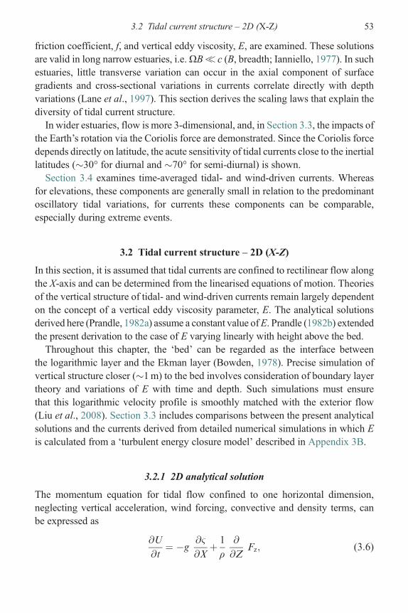
friction coefficient, f, and vertical eddy viscosity, E, are examined. These solutionsare valid in long narrow estuaries, i.e.ΩB≪ c (B, breadth; Ianniello, 1977). In suchestuaries, little transverse variation can occur in the axial component of surfacegradients and cross-sectional variations in currents correlate directly with depthvariations (Lane et al., 1997). This section derives the scaling laws that explain thediversity of tidal current structure.In wider estuaries, flow is more 3-dimensional, and, in Section 3.3, the impacts of

the Earth’s rotation via the Coriolis force are demonstrated. Since the Coriolis forcedepends directly on latitude, the acute sensitivity of tidal currents close to the inertiallatitudes (�30° for diurnal and �70° for semi-diurnal) is shown.Section 3.4 examines time-averaged tidal- and wind-driven currents. Whereas

for elevations, these components are generally small in relation to the predominantoscillatory tidal variations, for currents these components can be comparable,especially during extreme events.

3.2 Tidal current structure – 2D (X-Z)

In this section, it is assumed that tidal currents are confined to rectilinear flow alongthe X-axis and can be determined from the linearised equations of motion. Theoriesof the vertical structure of tidal- and wind-driven currents remain largely dependenton the concept of a vertical eddy viscosity parameter, E. The analytical solutionsderived here (Prandle, 1982a) assume a constant value ofE. Prandle (1982b) extendedthe present derivation to the case of E varying linearly with height above the bed.Throughout this chapter, the ‘bed’ can be regarded as the interface between

the logarithmic layer and the Ekman layer (Bowden, 1978). Precise simulation ofvertical structure closer (�1m) to the bed involves consideration of boundary layertheory and variations of E with time and depth. Such simulations must ensurethat this logarithmic velocity profile is smoothly matched with the exterior flow(Liu et al., 2008). Section 3.3 includes comparisons between the present analyticalsolutions and the currents derived from detailed numerical simulations in which Eis calculated from a ‘turbulent energy closure model’ described in Appendix 3B.

3.2.1 2D analytical solution

The momentum equation for tidal flow confined to one horizontal dimension,neglecting vertical acceleration, wind forcing, convective and density terms, canbe expressed as

@U

@t¼ �g

@&

@Xþ 1

ρ@

@ZFz; (3:6)

3.2 Tidal current structure – 2D (X-Z) 53

where Fz is the component of frictional stress exerted at level Z by the water abovethat level. Expressing the frictional stress in terms of a (constant) vertical eddyviscosity, E, gives

Fz ¼ ρ E@U

@Z: (3:7)

Limiting consideration to a single tidal constituent of frequency, ω, at any position,we assume

Uðz; tÞ ¼ Re½UðZÞeiωt� (3:8)

and

ζ ðtÞ ¼ Re½Weiωt�; (3:9)

where U(Z) and W take a complex form to reflect tidal phase variations.Substituting (3.7), (3.8) and (3.9) into (3.6), we can eliminate the time variation

eiωt to give

iωU ¼ �g@

@XWþ E

@2

@Z2U: (3:10)

Equation (3.10) is satisfied by the solution

U ¼ A1ebz þ A2e

�bz þ C (3:11)

with

b ¼ iωE

� �1=2and C ¼ �g

iω@

@XW: (3:12)

Boundary conditions

At the surface Z=D, the frictional stress Fz = 0, i.e.

A1b ebD � A2b e

�bD ¼ 0

or A1 ¼ A2 e�2bD: (3:13)

At the bed Z= 0, we assume the stress described by (3.7) is equal to the stressdescribed by the linearised quadratic friction law, Section 2.5 (Proudman, 1953,p. 316),

E ðA1b� A2bÞ ¼ 8

3πf U � Uz¼0 ¼ 8

3πf U� ðA1 þ A2 þ CÞ; (3:14)

where U* represents the depth-averaged tidal amplitude.

54 Currents

Continuity

The total flow is given by

U�D ¼ðD

0

U dZ ¼ A1

bebD � 1� �� A2

be�bD � 1� �þ CD: (3:15)

Velocity profiles

Combining (3.11) to (3.15), we obtain the following solution for the velocity U atany height Z,

UðzÞU� ¼ ðebZ þ e�bZþ2yÞ

TþQ; (3:16)

where T ¼ ð1� e2yÞ j� 1

y� 1

� �� 2 e2y (3:17)

and Q ¼ jð1� e2yÞ � 1� e2y½ �T

(3:18)

j ¼ 3 π E b

8 fjU�j (3:19)

y ¼ bD: (3:20)

Letting j = J i½ and y = Y i½, we obtain

J ¼ 3πðEωÞ1=28 f U� (3:21)

and Y ¼ ωE

� �1=2

D: (3:22)

3.2.2 Comparisons with observations

The velocity profile described by (3.16) is a function of two variables, J and Y.Y may be interpreted as a depth parameter converted to a dimensionless form byEkman scaling (Faller and Kaylor, 1969; Munk et al., 1970). J is also dimensionlessand reflects the effect of the quadratic bottom stress through the bed-stress coeffi-cient f and the depth-averaged velocity amplitude U*. It may be shown from (3.16)that when J is large, the velocity distribution is always uniform through depth.For large values of Y, the solution (3.16) approaches an asymptote that is a function

3.2 Tidal current structure – 2D (X-Z) 55

of J only. Thus, the full range of vertical tidal current structure is represented by theparameter ranges 0 < Y< 5 and 0 < J< 10.Figure 3.1 shows, in contour form, the ratio of the velocity at the bed to the

depth-averaged velocity, i.e. |UZ= 0/U*| plotted as a function of Y and J. It alsoshows the phase difference Δθ= θs− θb between velocities at the surface and bed,with Δθ< 0 indicating a phase advance at the bed. Pronounced vertical structureoccurs in the range Y> 1 and J< 2. This latter point is emphasised by Fig. 3.2(Prandle, 1982a) where complete velocity profiles are shown for co-ordinate values,(J, Y)= (a) (0.5,5); (b) (5,5); (c) (0.5,0.5) and (d) (5,0.5).The profiles described by the above theory correspond in character with mea-

sured profiles for tides in rivers, estuaries and shallow seas (Van Veen, 1938). Thedepthmean velocity occurs at a fractional height (z=Z/D), 0.25 < z< 0.42 – validatingthe common engineering assumption that average velocity occurs close to 0.4Dabove the bed. Velocities measured at z=0.4D will provide an estimate of the depthmean value with a maximum error of 4% in amplitude and 1.5° in phase.

0.45

4

3

2

1

01 2 3 4 5

J

y

6 7 8 9 10

0.5 0.6 0.7 0.8 0.9

0.95

Fig. 3.1. Surface to bed differences in amplitude and phase of tidal currents as f(J, Y). (Left) Velocity at the bed as a fraction of the depth-averaged value. (Right)Phase differences between velocities at the surface and bed (negative valuesindicate phase advance at the bed).

56 Currents

The maximum velocity generally occurs close to the surface. However, for Y >4maximum velocity occurs below the surface, and for Y� 5 maximum velocity occursat mid-depth.

3.2.3 Eddy viscosity formulation, Strouhal number

A fuller interpretation of the above theory requires some formulation for eddyviscosity. Two commonly assumed expressions in dimensionally consistent form are

E ¼ αU�D (3:23)

E ¼ βU� 2

ω: (3:24)

Bowden (1953) suggested a formulation similar to (3.23) while Kraav (1969)suggested a formulation similar to (3.24). Substituting (3.23) into (3.21) and(3.22) we obtain

Y ¼ 8

3πfJ

α: (3:25)

5–40°

–30°–20°

–10°

–5°

–1°

4

3

2

1

01 2 3 4 5

J

y

6 7 8 9 10

Fig. 3.1. (cont.)

3.2 Tidal current structure – 2D (X-Z) 57

Similarly, substituting (3.24) into (3.21) gives

J ¼ β1=2

8=3πf: (3:26)

McDowell (1966) presents values of the phase difference θ between surface andbed found for oscillatory flows in a laboratory flume, showing that θ increasescontinuously as the parameter f SR decreased, where SR =U P/D is the Strouhalnumber. Prandle (1982a) showed that these data correspond to Y= 1.7J, thussupporting Bowden’s (1953) formulation for eddy viscosity and from (3.25) sug-gesting a value of α� 0.5f. Using E= α0 | Uz= 0 | D, Bowden found values of α0 inthe range 0.0025–0.0030, thus agreement with the present value for α requires

–20°1.0

0.5Z /D

0 0.5(a) (b)

(c) (d)

1.0

–10° 0° 10° 20°θ

θ

–20°1.0

0.5

0 0.5 1.0

–10° 0° 10° 20°

θ

θ

0.5

–20°1.0

0.5Z /D

0 1.0

–10° 0° 10° 20°θ

θ

Uz = 0 / U�

–20°1.0

0.5

0 0.5 1.0

–10° 0° 10° 20°θ

θ

Uz = 0 / U�

Fig. 3.2. Vertical structure of current amplitude and phase as f (J, Y). Profiles for(J, Y) = (a) (0.5, 5.0), (b) (5.0, 5.0), (c) (0.5, 0.5) and (d) (5.0, 0.5).

58 Currents

|Uz = 0 /U |� 0.5. Prandle (1982b) showed that analytical solutions of (3.6) requireE> 0.5fU*D.Bowden’s (1953) formulation is appropriate in most estuaries when the boundary

layer thickness extends to the surface, whereas in deeper water, Kraav’s (1969)formulation applies. Davies and Furnes (1980) used the latter formulation inmodelling tidal current structure in depths of up to 200m over the UK continentalshelf area.By assuming Bowden’s (1953) formulation for eddy viscosity, with α = f, the

vertical structure (3.16) reduces to a function of the single parameter f SR,with Y� 0.83J� 50/SR

1/2. Figure 3.3 (Prandle, 1982a) shows the resultant ver-tical structure as a function of SR for the case of f = 0.0025. For small values ofSR, i.e. SR < 50, the current structure is uniform except for a small phase advanceclose to the bed. For larger values of SR, the variation in current amplitudeincreases continuously, approaching an asymptote in the region of SR = 1000.The phase variation also increases with increasing SR but reaches a maximumdifference between surface and bed in the region of SR = 350. Thereafter, thephase variation decreases with increasing SR with only 1° difference betweensurface and bed for SR = 10 000. The phase variation is generally concentratedclose to the bed except when 100 < SR < 1000.In a typical strongly tidal estuary with anM2 tidal current amplitudeU*� 1ms−1,

SR > 1000 for D< 40m, and thus the vertical structure will tend towards the asymp-totic solution for large SR shown in Fig. 3.3.

3.3 Tidal current structure – 3D (X-Y-Z)

The fundamental difference in extending the above theory for uni-directional to fully3D currents is the inclusion of the Coriolis force in the momentum equation (3.6).Although for the major tidal constituents in many estuaries, thedepth-integrated effect of this term may be of second order, the (differential)influence on vertical structure can be highly significant.

3.3.1 Tidal ellipse resolved into clockwiseand anti-clockwise components

In a horizontal plane, tidal current vectors rotate and, relative to a fixed origin,describe an elliptical path. A common practice is to resolve the ellipse into twocircular motions, one rotating clockwise (R2, g2) and the other anti-clockwise(R1, g1). Appendix 3A provides a fuller description of this transformation. In vectornotation with X the real axis and Y the orthogonal complex axis, the tidal vector, R,is given by

3.3 Tidal current structure – 3D (X-Y-Z) 59

R ¼ Uþ iV: (3:27)

Resolving R into a clockwise component R2 and an anti-clockwise componentR1 (|R1| and |R2| constant),

R ¼ R1 þ R2: (3:28)

1.0

1.14

1.10

1.07

1.03

1.00

0.90

0.80

0.700.64

1.18

1.01

0.8

0.6

Z /D

Z /D

0.4

0.2

0

1.0

0.8

0.6

0.4

0.2

010 100

s

(b)

1000 10 000

10 100 s

(a)

1000

–5°

–4°–3°

–2°

–1°

1°

2°

3°4°

5°6°

7°8°

0°

10 000

Fig. 3.3. Current profile as a function of the Strouhal number, SR =U* P/D.(a) amplitude U(z)/Umean; (b) phase structure θ(z) – θmean.

60 Currents

3.3.2 3D analytical solution

The linearised equations of motion for flow in two dimensions may be written as

@U

@t�ΩV ¼ �g

@&

@Xþ 1

ρ@

@ZFzx (3:29)

and

@V

@tþΩU ¼ �g

@&

@Yþ 1

ρ@

@ZFzy; (3:30)

whereΩ is the Coriolis parameter and Fzx and Fzy are the components of Fz along Xand Y. These equations can be transformed using (3.27) and (3.28) into the followingequations for the separate rotational components:

anti-clockwise i ðΩþ ωÞ R1 ¼ G1 þ @

@ZE

@

@ZR1 (3:31)

clockwise i ðΩ� ωÞ R2 ¼ G2 þ @

@ZE

@

@ZR2; (3:32)

where G1 and G2 are rotational components of the surface gradient.Comparing (3.31) and (3.32) with (3.10) we see that for E constant through depth,

the equations are analogous. Thus, the solutions will be equivalent with the impor-tant difference that for the anti-clockwise component

b ! B1 ¼ i ðΩþ ωÞE

� 1=2; (3:33)

while for the clockwise component

b ! B2 ¼ i ðΩ� ωÞE

� 1=2: (3:34)

For Ω>ω, the resulting velocity profiles can be deduced directly from the 1Dprofiles described previously by simply replacing ω by ω0 =Ω ±ω. For Ω<ω, theclockwise parameter B2 may be rewritten in the form

B 02 ¼ i

i ðω� ΩÞE

� 1=2: (3:35)

From (3.11), velocity structure is dependent on exp(±bZ) then noting that

ei1=2q ¼ ðeiq2Þ1=2; (3:36)

whereas

3.3 Tidal current structure – 3D (X-Y-Z) 61

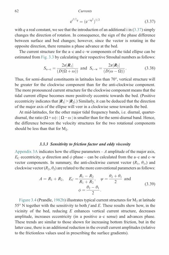
ei3=2q ¼ ðe�iq2Þ1=2 (3:37)

with q a real constant, we see that the introduction of an additional i in (3.37) simplychanges the direction of rotation. In consequence, the sign of the phase differencebetween surface and bed changes; however, since the vector is rotating in theopposite direction, there remains a phase advance at the bed.The current structure for the a–c and c–w components of the tidal ellipse can be

estimated from Fig. 3.3 by calculating their respective Strouhal numbers as follows:

Sa�c ¼ 2π R1j jD Ωþ ωð Þð Þ and Sc�w ¼ 2π R2j j

D ω�Ωð Þð Þ : (3:38)

Thus, for semi-diurnal constituents in latitudes less than 70°, vertical structure willbe greater for the clockwise component than for the anti-clockwise component.The more pronounced current structure for the clockwise component means that thetidal current ellipse becomes more positively eccentric towards the bed. (Positiveeccentricity indicates that |R1| > |R2|.) Similarly, it can be deduced that the directionof the major axis of the ellipse will veer in a clockwise sense towards the bed.At mid-latitudes, for the other major tidal frequency bands, i.e. diurnal, quarter-

diurnal, the ratio (Ω+ω) : |Ω−ω | is smaller than for the semi-diurnal band. Hence,the difference between the velocity structures for the two rotational componentsshould be less than that for M2.

3.3.3 Sensitivity to friction factor and eddy viscosity

Appendix 3A indicates how the ellipse parameters – A amplitude of the major axis,EC eccentricity, ψ direction and � phase – can be calculated from the a–c and c–wvector components. In summary, the anti-clockwise current vector (R1, θ1,) andclockwise vector (R2, θ2) are related to the more conventional parameters as follows:

A ¼ R1 þ R2; EC ¼R1 � R2

R1 þ R2

; ψ ¼ θ2 þ θ12

and

� ¼ θ2 � θ12

:

(3:39)

Figure 3.4 (Prandle, 1982b) illustrates typical current structures for M2 at latitude55° N together with the sensitivity to both f and E. These results show how, in thevicinity of the bed, reducing E enhances vertical current structure, decreasesamplitude, increases eccentricity (in a positive a–c sense) and advances phase.These trends are similar to those shown for increasing bottom friction, but in thelatter case, there is an additional reduction in the overall current amplitudes (relativeto the frictionless values used in prescribing the surface gradients).

62 Currents

3.3.4 Sensitivity to latitude

Figure 3.5 (Prandle, 1997) shows solutions for (3.31) and (3.32) as functions oflatitude and water depth for surface gradients which correspond to a ‘free stream’

rectilinear tidal current R* = 0.32m s−1. (Free stream corresponds to the solution of(3.31) and (3.32) with D infinite or f zero, i.e. in deep, frictionless conditions.) Thefigure emphasises the enhanced influence of the friction term at latitudes corre-sponding to the inertial frequency, i.e. for M2: sin

−1(24/2/12.42)� 75°.Figure 3.6 (Prandle, 1997) extends these results using simulations by Prandle

(1997), from (A) a 2D vertically averaged model and (B) a 3D model incorporatinga Mellor and Yamada (1974) level 2.5 closure scheme as described in Appendix 3B.The simulations cover a range of R*= 0.1, 0.32 and 1.0m s−1. The contour valuesshown are restricted to |R| = 0.9R*, phase and direction = ±10° and eccentricity =±0.1. These can be regarded as representative boundaries between conditions wheretidal propagation is little influenced by friction (in deeper water) and conditionswhere bottom friction becomes increasingly significant (in shallower water).

(a)

(b)

0° –10° –20° –30°–40°φ

0.20 0.4

Ec

0° –10° –20° –30°–40°φ

1.0

0.5

Z0

00 0.5

A

A

ε0 = 0.1

ε0 = 0.5

ε0 = 0.05

1.0 0.20 0.4Ec

0° –10° –20° –30°ψ

ε0 = 0.1

ε0 = 0.5

ε0 = 0.05

Z0

kW0 = 0.4 kW

0 = 0.1

kW0 = 0.02

1.0

0.5

00 0.5 1.0 0° –10° –20° –30°

ψ

kW0 = 0.4

kW0 = 0.1

kW0 = 0.02

Fig. 3.4. Sensitivity of current structure to eddy viscosity and bed friction.A amplitude, Ec eccentricity, ψ direction and � phase.(a) Eddy viscosity E= ε0D

2Ω, ε0 = 0.05, 0.1 and 0.5 (kW0 = 0.1).(b) Bed stress τ= ρfU*U, fU* = kW0ΩD, kW0 = 0.02, 0.1 and 0.4 (ε0 = 0.1).Results for M2 amplitude of 1m s−1 at latitude 55° N.

3.3 Tidal current structure – 3D (X-Y-Z) 63

The qualitative agreement for depth-averaged ellipse parameters between the2D and 3D models indicates how in deeper water these results are very close, whilein shallow water, by suitable adjustment of the bed friction coefficient, 2D modelresults can be adjusted to approximate those of 3Dmodels. It was shown in Section 2.5that for a predominant tidal constituent, i, the quadratic friction term f Ri Ri| can belinearised (in one dimension) to (8/3π) f Ri Ri* (where Ri* is the tidal amplitude). Theequivalent linearisation for other constituents, j, is (4/π) f RjRi*. Thus, the frictionaleffect is linearly proportional to f Ri* for all constituents, and thus any enhancementof f to improve reproduction of the primary constituent in a 2D model should notadversely affect other constituents. The results shown in Fig. 3.6 for f=0.0125 areincluded as an illustration of an enhanced frictional coefficient applicable for asecondary constituent factored by 3/2 Ri*/Rj* in such simulations.

3.3.5 Surface to bed changes in tidal ellipses

Figure 3.7 (Prandle, 1997) indicates the changes in current ellipse parameters betweenthe surface and the bed as calculated frommodels: (B) the level 2.5 closure k–ɛmodel

0.5

0.5

60°

30°

10 25 50Depth (m)

Depth (m)

100

Amplitude

Direction Eccentricity

Latitude

200

10 25 50 100 200

0°

0.6

0.4

0.7

0.3

0.8

0.2

0.9

0.1

0.01

320°

320°

330°

330°

340°

340°

350°

350°

60°

60°

30°

30°

10 25 50Depth (m)

100

Phase

Latitude

Latitude Latitude

200

10 25 50Depth (m)

100 200

0°

0°

60°

30°

0°

Fig. 3.5. Modulation of depth-averaged M2 ellipse due to bed friction, as f (Depth,Latitude). Contours show changes (fractional for amplitude R = 0.32m s−1) relativeto frictionless values of zero eccentricity, phase and direction.

64 Currents

Fig. 3.6. Modulation of depth-averaged M2 ellipse parameters by friction in 2D and3D models.(Left) Bed friction in a 2D model;(Right) bed friction and vertical eddy viscosity (MY 2.5) in a 3D model.Contours show: – amplitude 0.9, - - - - phase 350°, –––– direction 350°, …….eccentricity 0.1 and –– bed friction coefficient f×5= (0.0125). For frictionlessR*=0.1(top), 0.32 (middle), 1.0 (bottom) ms−1.

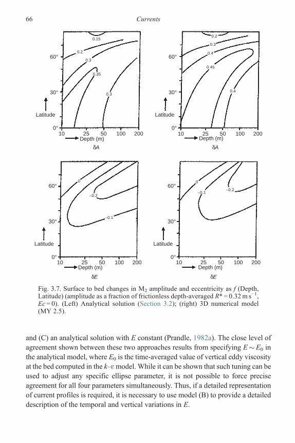
and (C) an analytical solution with E constant (Prandle, 1982a). The close level ofagreement shown between these two approaches results from specifying E�E0 inthe analytical model, where E0 is the time-averaged value of vertical eddy viscosityat the bed computed in the k–ɛmodel. While it can be shown that such tuning can beused to adjust any specific ellipse parameter, it is not possible to force preciseagreement for all four parameters simultaneously. Thus, if a detailed representationof current profiles is required, it is necessary to use model (B) to provide a detaileddescription of the temporal and vertical variations in E.

0.150.2

0.3

0.4

0.45

0.4

0.2

0.3

0.3

0

–0.2

–0.1

0

–0.2–0.1

100°

30°

Latitude

60°

25Depth (m)

δA

50 100 200

100°

30°

Latitude

60°

25Depth (m)

δE

50 100 200 100°

30°

Latitude

60°

25Depth (m)

δE

50 100 200

100°

30°

Latitude

60°

25Depth (m)

δA

50 100 200

0.35

Fig. 3.7. Surface to bed changes in M2 amplitude and eccentricity as f (Depth,Latitude) (amplitude as a fraction of frictionless depth-averaged R* = 0.32m s−1,Ec = 0). (Left) Analytical solution (Section 3.2); (right) 3D numerical model(MY 2.5).

66 Currents

The mean depth-averaged value of E calculated from the k–ɛ model (B) istypically four times larger than the value at the bed E0, and thus specifying this inmodel (C) significantly reduces the vertical structure shown in Fig. 3.7.

3.3.6 Currents across the inter-tidal zone

Successive wetting and drying of inter-tidal areas can generate significant cross-shore currents. If it is assumed that such currents are the primary source of in-fillingand draining, then tidal current speeds over a uniform bank slope SL will havean amplitude of ως*. /SL, where ς* is the amplitude of the surface elevation. For asemi-diurnal current, this corresponds to a maximum cross-shore current amplitudeof 7 cm s−1 for every kilometre of exposed bank. Prandle (1991), shows, from bothmodelling simulations and H.F. Radar observations, how such currents overinter-tidal zones modify tidal ellipse characteristics in the near-shore zone.

3.4 Residual currents

Removal of the oscillatory tidal component from current observations leavesresiduals that may include contributions from ‘rectified’ tidal propagation, direct(localised) wind forcing, indirect (larger scale) wind forcing, surface waves andhorizontal and vertical density gradients. Interaction of any of these componentswith the tidal component can generate significant modulation of the latter, contri-buting an additional non-tidal residual. Selective filtering of the non-tidal currentsinto frequency bands can be used to separate many of these components.Density-driven residual currents are described in Chapter 4. Soulsby et al. (1993)

provide a review of the nature and impact of current interaction with surface waves,quantifying the effect on the bed friction coefficient. Wolf and Prandle (1999)indicate how, in shallow water, such wave impacts can substantially reduce tidalcurrents.

3.4.1 Wind-driven currents

Relating observed wind-driven currents to wind forcing is notoriously difficult.Both the wind itself and the associated currents exhibit appreciable fine-scale(temporal and spatial) variability. In shallower water, wind forcing may be partiallybalanced by surface slopes. In constricted cross sections, these slopes can sub-sequently generate currents which are orders of magnitude greater than indicatedby direct localised surface wind forcing (Prandle and Player, 1993).The response of the sea surface to surface wind forcing under steady-state

conditions was originally studied by Ekman; a convenient summary of results is

3.4 Residual currents 67

given by Defant (1961). The essential features can be described by considering asteady-state solution to (3.31) and (3.32) (Prandle and Matthews, 1990). Thusrewriting these equations in the form

iΩR þ S ¼ E@2R

@Z2; (3:40)

where S is the surface gradient term and E the vertical eddy viscosity is assumedconstant.Surface (Z=D) and bed (Z= 0) boundary conditions are, respectively,

τw ¼ ρ E@R

@Z(3:41)

ρ F Rz¼0 ¼ ρ E@R

@Z; (3:42)

where τw is the surface wind stress and F Rz = 0 a (linearised) representation of bedfriction.A solution in the form of an Ekman spiral,

R ¼ A ebz þ C; (3:43)

is satisfied by

RðzÞ ¼ τwρEb ebD

ebz þ Eb

F� 1

� �; (3:44)

where b2 = i (Ω/E).In deeper water, bD≫ 1, i.e. D≫ (E/Ω)½, the first term in (3.44) predomi-

nates and

Rz¼D ¼ �τw i1=2

ρ ðΩE Þ1=2; (3:45)

i.e. a surface current of magnitude dependent on latitude and veering at 45° clock-wise to the wind stress.In shallow water, the second term predominates and

R ¼ τw e�bD

ρF; (3:46)

i.e. a current of magnitude dependent on the bed friction coefficient and aligned withthe wind.Figure 3.8 shows these wind-driven surface-current responses derived from

statistical analyses of H.F. Radar observations (Prandle and Matthews, 1990).

68 Currents

Substituting (3.4) for wind stress, τ, yields a response in close agreement with thatshown from the Radar observations in Fig. 3.8. The steady-state surface currents aretypically 1 or 2% of wind speed, increasing in deeper water in both magnitude andveering towards the theoretical deep water values of 45° to the right of the wind. Theobserved veering ranges from 3° to 35° (clockwise).

3.4.2 Tidal current residuals

The mechanisms by which tidal energy propagating into estuaries at semi-diurnaland diurnal periods generate higher-order harmonics and residual components isdescribed in Section 2.6. It was shown how determination of residual currents iscomplicated by which parameter is defined to be the (linear) controlling factor.In shallow water, calculation of residual current components is further complicatedby the respective reference systems, e.g. fixed distances above the bed or below thesurface, fractional heights. The continuous profile provided by an Acoustic DopplerCurrent Profiler (ADCP) allows observational data to be readily interpolated onto

Fig. 3.8.Wind-driven surface current for a wind of 1m s−1 eastwards. Derived fromH.F. Radar measurements.

3.4 Residual currents 69

the selected vertical framework. However, for residual and higher harmonics,derived values are especially sensitive to the prescribed framework (Lane et al.,1997).An Euler current at a fixed height above the bed corresponds to the velocity

observed by a moored current meter. The tidally averaged, depth-integrated Eulerresidual is defined as

UE ¼ 1

P

ðP

0

1

Dþ &

ðDþ&

0

UðZÞ dZ0@

1A dt: (3:47)

The tidally averaged, depth-integrated, residual transport current is

UT ¼ 1

DP

ðP

0

ðDþ&

0

UðZÞ dZ0@

1A dt (3:48)

with UT D=Q, the river flow per unit breadth.For uniform flow of a single tidal constituent in one direction, the difference

between the above residual current components is

UT ¼ UE þ 0:5 &� U�=D cos ðθÞ; (3:49)

where θ is the phase difference between ζ andU and the second term is referred to asthe Stokes’ drift. Cheng et al. (1986) provide further details of the differencebetween Eulerian and Lagrangian flows in non-uniform flow fields.Prandle (1975) showed that the depth-integrated net energy propagation can be

approximated by

EN ¼ ρgD 0:5 &� U� cosðθÞ½ �: (3:50)

This implies that net propagation of tidal energy will be accompanied by a smallresidual Stokes’ drift. In open seas, this can produce a persistent residual circulation.Amodelling study by Prandle (1984) showed typical residual currents of 1–3 cm s−1

in the continental shelf around the UK. However, in an enclosed estuary, somecompensating outflow must be present, as noted in Section 2.6.3.As an example of these persistent tidally driven residual currents, Fig. 3.9 shows a

residual surface current gyre measured in a year-long H.F. Radar deployment inthe Dover Strait (Prandle and Player, 1993). Such gyres are not exceptional butrather a characteristic of most coastlines, although rarely identified with conven-tional instruments. Geyer and Signell (1991) mapped a similar headland gyre with avessel-mounted ADCP.

70 Currents

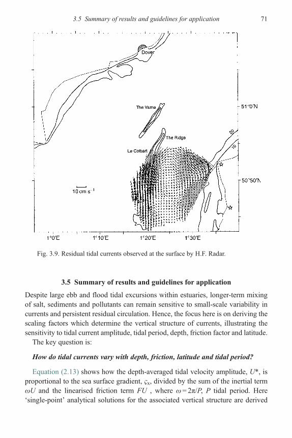
3.5 Summary of results and guidelines for application

Despite large ebb and flood tidal excursions within estuaries, longer-term mixingof salt, sediments and pollutants can remain sensitive to small-scale variability incurrents and persistent residual circulation. Hence, the focus here is on deriving thescaling factors which determine the vertical structure of currents, illustrating thesensitivity to tidal current amplitude, tidal period, depth, friction factor and latitude.The key question is:

How do tidal currents vary with depth, friction, latitude and tidal period?

Equation (2.13) shows how the depth-averaged tidal velocity amplitude, U*, isproportional to the sea surface gradient, ςx, divided by the sum of the inertial termωU and the linearised friction term FU , where ω= 2π/P, P tidal period. Here‘single-point’ analytical solutions for the associated vertical structure are derived

Fig. 3.9. Residual tidal currents observed at the surface by H.F. Radar.

3.5 Summary of results and guidelines for application 71

for specified values of ςx. For the case of a constant eddy viscosity, E, this verticalstructure is shown to be determined by two parameters Y=D(ω/E)1/2 and J= 3π(Eω)1/2/8 f U* (D water depth and f bed friction coefficient). Y is analogous to anEkman height and J introduces the effect of bed friction.From both comparisons of observed structure against these solutions and self-

consistency of the analytical solutions, the approximation E= f U*D is shown to bevalid in strongly tidal, shallow waters where the influence of the bottom boundarylayer extends to the surface. Figure 3.7 shows a comparison of tidal current structuresdetermined using this constant value for E versus detailed numerical simulationsemploying a turbulence closure module (Appendix 3B). The overall level of agree-ment indicates the validity of the approximation.Adopting this approximation for E, the characteristics of vertical structure of tidal

currents can be reduced to dependency on the Strouhal number, SR =UP/D withY� J� 50/SR

1/2 for f = 0.0025. The amplitude structure becomes more pronouncedwith increasing SR up to an asymptotic limit of SR� 350. Accompanying phasevariations are a maximum for this value of SR but decrease for both smaller andlarger values (Fig. 3.3). In meso- andmacro-tidal estuaries, the Strouhal number willbe well in excess of 1000.Commonly observed features explained by this theory include, Figs. 3.1 and 3.3:

(1) depth-mean velocity occurring at fractional height (z= Z/D) above the bed, z= 0.4;(2) phase advance at the bed relative to the surface of up to 20° (at SR� 350). A similar

phase advance at the coastal boundaries relative to the deep mid-section generallyoccurs.

(3) maximum velocities occurring at the surface, except for Y> 4 (SR < 300) where sub-surface maxima occur (although not especially pronounced).

The above solutions ignore the effects of the Earth’s rotation represented by theCoriolis term in (2.1) and (2.2). Even in long narrow estuaries, the Coriolis term issignificant in determining the details of tidal current structure. This significance can beunderstood by noting that tidal currents do not simply ebb and flood along one axis butrotate in an elliptic pattern. The characteristics of these ellipses are represented by theparameters: AMAX amplitude along the principal axis, AMIN amplitude along the(orthogonal) minor axis, ψ direction of the principal axis, φ phase (time of maximumcurrent). The eccentricity EC=AMIN/AMAX with the additional convention of positivefor anti-clockwise (a–c) rotation and negative for clockwise (c–w).Vertical variations in these ellipse parameters calculated from observations can

often appear bewilderingly complex. However, an underlying systematic structureinvariably emerges when the ellipse is separated into its clockwise and anti-clockwise rotational components. (1D flow corresponds to EC =AMIN = 0 andoccurs when the magnitude of the two rotational components are equal). This

72 Currents

separation enables the influence of the Coriolis term to be directly illustrated. Thus,expanding the above theory to include the Coriolis term introduces separateStrouhal Numbers for each rotational component as follows:

Sa�c ¼ 2πUDðωþ ΩÞ and Sc�w ¼ 2πU

Dðω� ΩÞ : (3:51)

For a semi-diurnal constituent, ω� 1.4 × 10−4, while at a latitude of 50°, the Coriolisterm Ω� 1.1 × 10−4. Thus, for such conditions, we see that the c–w Strouhal numberis generally an order of magnitude greater than the a–c value. This results in a muchmore pronounced vertical structure for the c–w component and directly explains thecommonly observed features of

(1) increasing c–w eccentricity towards the surface(2) major axis veering a–c towards the surface.

The acute sensitivity of tidal currents close to inertial latitudes, where ω=Ω(�70° for semi-diurnal constituents and �30° for diurnal), is shown in Fig. 3.5.Although this may be qualified by evidence from Csanady (1976) that the thicknessof the boundary layer and in consequence the vertical eddy viscosity is itself relatedto the Coriolis parameter.The above mathematical approach used in determining the details of tidal current

structure can be usefully applied to derive the steady-state vertical current structureassociated with wind forcing (3.44). This theory explains the observed ‘Ekmanspiral’ patterns of wind-driven currents shown in Fig. 3.8. Maximum surfacecurrents, up to a few percent of the wind speed, occur in deep water, veering 45°to the right of the wind (northern hemisphere). In shallowwater, bed friction reducesthese currents and aligns them more closely with the wind direction.

Appendix 3A

3A.1 Tidal current ellipse

Figure 3A.1 (Prandle, 1982b) illustrates how a current ellipse may be resolved intotwo rotary components. The current vectors are shown at time t= 0.On the left, the anti-clockwise rotating component is given by

R1 ¼ R1j jðcos g1 þ i sin g1Þ: (3A:1)

In the middle, the clockwise rotating component is

R2 ¼ R2j jðcos g2 þ i sin g2Þ: (3A:2)

The maximum current occurs at time tMAX when R1 and R2 are aligned, i.e. when

Appendix 3A 73

ωtMAX þ g1 ¼ �ωtMAX þ g2

or tMAX ¼ g2 � g12ω

: (3A:3)

The phase, φ, is given by

j ¼ ωtMAX (3A:4)

and the maximum amplitude, AMAX, is

AMAX ¼ R1j j þ R2j j: (3A:5)

The inclination, ψ, of the maximum current to the X-axis is given by

ψ ¼ ωtMAX þ g1 ¼ �ωtMAX þ g2 ¼1

2ðg2 þ g1Þ: (3A:6)

The minimum amplitude, AMIN, is when R1 and R2 are opposed, hence

AMIN ¼ R1j j � R2j jj j: (3A:7)

The eccentricity of the ellipse, Ec, is defined as the ratio AMIN:AMAX. However, inaddition, we use the convention of Ec positive for anti-clockwise current rotation|R1| > |R2| and negative for clockwise rotation, | R2| > |R1|. Thus letting μ= |R1|/| R2|,we define Ec as follows:

Ec ¼ μ� 1

μþ 1: (3A:8)

Hence, | Ec | is a minimum when μ= 1 and | Ec | increases as μ increases above thisvalue.

y

x x x

yA

Ψ

y

R1

R2g1

g2

R1 R2 R = R1 + R2

wt

wt

Fig. 3A.1. Decomposition of a tidal current ellipse into anti-clockwise and clockwiserotating components.

74 Currents

Appendix 3B

3B.1 Turbulence model

The Mellor–Yamada level 2.5 mode (MYL 2 5, Mellor and Yamada (1974)) iswidely used to determine the values of the vertical eddy viscosity, KM, and verticaleddy diffusivity,Kq, coefficients. Refinements of thismodel described byDeleersnijderand Luyten (1993) are incorporated here. Umlauf and Burchard (2003) describe morerecent developments.The turbulent kinetic energy (TKE or k) equation is k= q2/2

@

@t

q2

2

� �¼ @

@ZKq

@

@Z

q2

2

� �� ðdiffusionÞ

þKM@U

@Z

� �2

þ @V

@Z

� �2" #

ðshear productionÞ

� q3

B1

¼ 0 ðdissipationÞ; (3B:1)

where B1 = 16.6 and the eddy coefficients are proportional to the mixing length l andassociated stability functions Sq and SH; thus

Kq ¼ lq; Sq ¼ 0:2lq (3B:2)

KM ¼ lq; SM ¼ 0:4lq: (3B:3)

The mixing length l is determined from the related equation

@

@tq2l ¼ @

@ZKq

@

@Zq2l� ��

þ E1l KM

@U

@Z

� �2

þ @V

@Z

� �2" #

�Wq3

B1

: (3B:4)

The wall proximity function W is defined as

W ¼ 1þ E2l2

KvLð Þ2 ; (3B:5)

where E1 = 1.8, E2 = 1.33. Kv is the van Karman constant (�0.4), and L is a functionof the distance to the seabed db and to the sea surface ds; thus

L ¼ ds dbds þ db

: (3B:6)

The boundary conditions specified at the surface and bed are

Appendix 3B 75

KM@R

@Z¼ τB

ρ(3B:7)

KM@R

@Z¼ τ0

ρ; (3B:8)

where the velocity R=U+ iV, τ0 is the applied wind stress and τB is the tidal stress atthe bed (ρfR|R|).At the surface and bed q2l= 0.

References

Bowden, K.F., 1953. Note on wind drift in a channel in the presence of tidal currents.Proceedings of the Royal Society of London, A, 219, 426–446.

Bowden, K.F., 1978. Physical problems of the Benthic Boundary Layer. GeophysicalSurveys, 3, 255–296.

Cheng, R.T., Feng, S., and Pangen, X., 1986. On Lagrangian residual ellipse. In: van deKreeke, J. (ed.), Physics of Shallow Estuaries and Bays (Lecture Notes on Coastal andEstuarine Studies No. 16) Springer-Verlag, Berlin, pp. 102–113.

Csanady, G.T., 1976. Mean circulation in shallow seas. Journal of Geophysical Research,81, 5389–5399.

Davies, A.M. and Furnes, G.K., 1980. Observed and computed M2 tidal currents in theNorth Sea. Journal of Physical Oceanography, 10 (2), 237–257.

Defant, A., 1961. Physical Oceanography, Vol. 1. Pergamon Press, London.Deleersnijder, E. and Luyten, P., 1993. On the Practical Advantages of the

Quasi-Equilibrium Version of the Mellor and Yamada Level 2–5 Turbulence ClosureApplied to Marine Modelling. Contribution No. 69. Institui d’Astronomie et deGeophysique, Universite Catholique de Louvain, Belgium.

Faller, A.J. and Kaylor, R., 1969. Oscillatory and transitory Ekman boundary layers.Deep-Sea Research, Supplement, 16, 45–58.

Flather, R.A., 1984. A numerical model investigation of the storm surge of 31 January and1 February 1953 in the North Sea. Quarterly Journal of the Royal MeteorologicalSociety, 110, 591–612.

Geyer, W.R. and Signell, R., 1991. Measurements and modelling of the spatial structure ofnonlinear tidal flow around a headland. In: Parker, B.B. (ed.), Tidal Hydrodynamics.John Wiley and Sons, New York, pp. 403−418.

Heaps, N.S., 1969. A two-dimensional numerical sea model. Philosophical TransactionsRoyal Society, London, A, 265, 93–137.

Ianniello, J.P., 1977. Tidally-induced residual currents in estuaries of constant breadth anddepth. Journal of Marine Research, 35 (4), 755–786.

Kraav, V.K., 1969. Computations of the semi-diurnal tide and turbulence parameters in theNorth Sea. Oceanology, 9, 332–341.

Lane, A., Prandle, D., Harrison, A.J., Jones, P.D., and Jarvis, C.J., 1997.Measuring fluxes inestuaries: sensitivity to instrumentation and associated data analyses. Estuarine,Coastal and Shelf Science, 45 (4), 433–451.

Liu, W.C., Chen, W.B., Kuo, J-T., and Wu, C., 2008. Numerical determination of residencetime and age in a partially mixed estuary using a three-dimensional hydrodynamicmodel. Continental Shelf Research, 28 (8), 1068–1088.

76 Currents

McDowell, D.M., 1966. Scale effect in hydraulic models with distorted vertical scale.Golden Jubilee Symposia, Vol. 2, Central Water and Power Research Station, India,pp. 15–20.

McDowell, D.M. and Prandle, D., 1972. Mathematical model of the River Hooghly.Proceedings of the American Society of Civil Engineers. Journal of Waterways andHarbours Division, 98, 225–242.

Mellor, G.L. and Yamada, T., 1974. A hierarchy of turbulence closure models for planetaryboundary layers. Journal of the Atmospheric Science, 31, 1791–1806.

Munk, W., Snodgrass, F., and Wimbush, M., 1970. Tides off-shore: Transition fromCalifornia coastal to deep-sea waters. Geophysical Fluid Dynamics, 1, 161–235.

Pingree, R.D. and Maddock, L., 1980. Tidally induced residual flows around an island dueto both frictional and rotational effects.Geophysical Journal of the Royal AstronomicalSociety, 63, 533–546.

Prandle, D., 1975. Storm surges in the southern North Sea and River Thames. Proceeding ofthe Royal Society of London, A, 344, 509–539.

Prandle, D., 1982a. The vertical structure of tidal currents and other oscillatory flows.Continental Shelf Research, 1, 191–207.

Prandle, D., 1982b. The vertical structure of tidal currents. Geophysical and AstrophysicalFluid Dynamics, 22, 29–49.

Prandle, D., 1984. A modelling study of the mixing of 137Cs in the seas of the Europeancontinental shelf. Philosophical Transactions of the Royal Society I of London, A, 310,407–436.

Prandle, D., 1991. A new view of near-shore dynamics based on observations fromH.F. Radar. Progress in Oceanography, 27, 403–438.

Prandle, D., 1997. The influence of bed friction and vertical eddy viscosity on tidalpropagation. Continental Shelf Research, 17 (11), 1367–1374.

Prandle, D., 2004. Saline intrusion in partially mixed estuaries. Estuarine, Coastal and ShelfScience, 59, 385–397.

Prandle, D. and Ryder, D.K., 1989. Comparison of observed (H.F. radar) and modellednear-shore velocities. Continental Shelf Research, 9, 941–963.

Prandle, D. and Matthews, J., 1990. The dynamics of near-shore surface currents generatedby tides, wind and horizontal density gradients. Continental Shelf Research, 10,665–681.

Prandle, D. and Player, R., 1993. Residual currents through the Dover Strait measured byH.F. Radar. Estuarine, Coastal and Shelf Science, 37 (6), 635–653.

Proudman, J., 1953. Dynamical Oceanography. Methuen and Co. Ltd, London.Soulsby, R.L., Hamm, L., Klopman, G., Myrhaug, D., Simons, R.R., and Thomas, G.P.,

1993. Wave–current interaction within and outside the bottom boundary layer. CoastalEngineering, 21, 41–69.

Souza, A.J. and Simpson, J.H., 1996. The modification of tidal ellipses by stratification inthe Rhine ROFI. Continental Shelf Research, 16, 997–1008.

Umlauf, L. and Burchard, H., 2003. A generic length-scale equation for geophysicalturbulence models. Journal of Marine Research, 6, 235–265.

Van Veen J., 1938. Water movements in the Straits of Dover. Journal du Conseil, ConseilInternational pour l’Exploration de la Mer, 14, 130–151.

Wolf, J. and Prandle, D., 1999. Some observations of wave–current interaction. CoastalEngineering, 37, 471–485.

Zimmerman, J.T.F., 1978. Topographic generation of residual circulation by oscillatory(tidal) currents. Geophysical and Astrophysical Fluid Dynamics, 11, 35–47.

References 77

4

Saline intrusion

4.1 Introduction

The nature of saline intrusion in an estuary is governed by tidal amplitude, river flowand bathymetry. The pattern of intrusion may be altered by ‘interventions’ such asdredging, barrier construction or flow regulation alongside impacts from changes inmsl or river flows linked to Global Climate Change. Adjustments to the intrusionmay have important implications for factors such as water quality, sedimentationand dispersion of pollutants. Whereas tidal propagation can be explained fromsimple analytical formula and accurately modelled, it is often difficult to explainobserved changes in intrusion from spring to neap or flood to drought.The laterally averaged mass conservation equation may be written as (Oey,

1984)

@C

@tþU

@C

@XþW

@C

@Z¼ 1

DB

@

@XDBKx

@C

@X

� �þD

@

@ZBKz

@C

@Z

� �� �; (4:1)

where C is concentration,U andW velocities in the axial X and vertical Z directions,D water depth, B breadth, Kx and Kz eddy dispersion coefficients. Lewis (1997)provides detailed descriptions of how advection and dispersion terms in (4.1) interactto promote estuarine mixing.Dispersion of salt involves interacting 3D variations in phase, amplitude andmean

values of both currents and the saline distribution. These variations are sensitiveto the level of density stratification which may vary appreciably – temporally andboth axially and transversally. The spectrum of such spatial and temporal variationsincludes

(1) the tidal cycle, with pronounced vertical mixing occurring on one or both of peak floodand ebb currents due to bottom friction, or at slack tides due to internal friction (Lindenand Simpson, 1988);

(2) the neap–spring cycle, with mixing occurring more readily on spring than neap tides;

78

(3) the hydrological cycle, with variations in both river flow and salinity of sea water at themouth (Godin, 1985);

(4) storm events including storm surges generated both internally and externally (Wangand Elliott, 1978) and surface wave mixing (Olson, 1986);

(5) variations in water density due to other parameters, in particular temperature(Appendix 4A) and suspended sediment load (Chapter 5).

This chapter does not consider the influence of temperature on density. AnAppendix is included describing the seasonal cycle of temperature variations as afunction of water depth and latitude. Nunes and Lennon (1986) indicate how evapora-tion at low latitudes can produce maximum salinities at the head of an estuary –

inverting the customary pattern of saline intrusion.

4.1.1 Classification systems

Pritchard (1955) introduced a classification scheme for estuarine mixing. In classA, ‘highly stratified estuaries’, the dispersion terms on the right-hand side of (4.1)are negligible. For type B, ‘partially mixed estuaries’, vertical dispersion is impor-tant. Types C, wide, and D, narrow, are ‘fully mixed estuaries’ with density profiles∂C/∂Z� 0 and hence only longitudinal dispersion is involved. This latter assertionis inconsistent with subsequent notions of mixing in well-mixed estuaries, forexample the role of tidal straining described in Section 4.4.While Pritchard’s classification system provides useful qualitative descriptions,

in many estuaries the degree of stratification varies appreciably both spatially andtemporally. Figure 4.1 shows a neap–spring time series of salinity variations at threedepths for a single location in the Mersey Estuary. While the tidal signals areevident, longer-term (sub-tidal) influences are much greater than for correspondingelevation or current time series. Figure 4.2 (Liu et al., 2008) shows how axialdistributions in the Danshuei River vary with changing river flows.The stratification diagram derived by Hansen and Rattray (1966) (Fig. 4.3) has

been used to classify the nature of mixing in estuaries and the sensitivity of thestratification to changing conditions. The diagram is based on two parameters: (i) δs/s,the salinity difference between bed and surface divided by the depth-averagedsalinity (mean values over a tidal cycle), and (ii) Us= �U residual velocity at thesurface divided by the depth-mean value. Four estuarine types are identified withsub-divisions into (a) mixed and (b) stratified according to whether δs/s is less orgreater than 0.1. In estuaries of type 1, residual flow is seawards at all depths andconsequently mixing of salt is entirely by diffusion. For type 2, residual flowreverses with depth and mixing is due to both advection and diffusion. For type 3,the vertical structure of the residual flow is so pronounced that advection accountsfor over 99% of the mixing process; in type 3(b), mixing is confined to the

4.1 Introduction 79

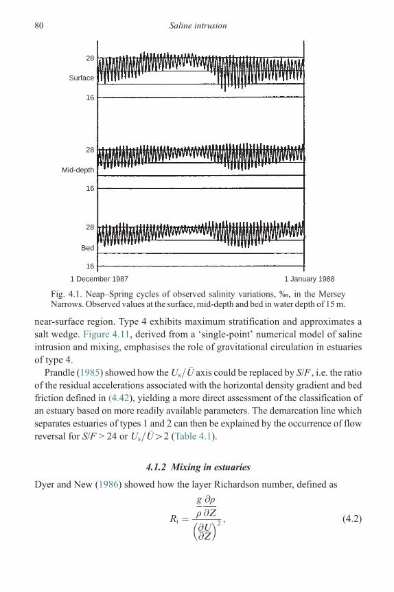
near-surface region. Type 4 exhibits maximum stratification and approximates asalt wedge. Figure 4.11, derived from a ‘single-point’ numerical model of salineintrusion and mixing, emphasises the role of gravitational circulation in estuariesof type 4.Prandle (1985) showed how theUs= �U axis could be replaced by S/F , i.e. the ratio

of the residual accelerations associated with the horizontal density gradient and bedfriction defined in (4.42), yielding a more direct assessment of the classification ofan estuary based on more readily available parameters. The demarcation line whichseparates estuaries of types 1 and 2 can then be explained by the occurrence of flowreversal for S/F > 24 or Us= �U42 (Table 4.1).

4.1.2 Mixing in estuaries

Dyer and New (1986) showed how the layer Richardson number, defined as

Ri ¼g

ρ@ρ@Z

@U@Z

� �2 ; (4:2)

28

16

Surface

28

16

Mid-depth

28

16

1 December 1987 1 January 1988

Bed

Fig. 4.1. Neap–Spring cycles of observed salinity variations, ‰, in the MerseyNarrows. Observed values at the surface, mid-depth and bed in water depth of 15m.

80 Saline intrusion

representing the ratio of buoyancy forces to vertical turbulent force, determinesthe nature of mixing in estuaries. Vertical mixing occurs forRi < 0.25when turbulenceis sufficient to overcome density layering. In determining whether an estuary is likelyto be mixed or stratified, the question arises as to which components of current shearpredominate (tidal, riverine or, circuitously, saline gradient-induced). Linden andSimpson (1988) and Simpson et al. (1990) have emphasised that stratification cannotbe simply linked to the ‘gross’ parameters used in (4.2). The value of Ri variesconsiderably along an estuary and over both the ebb–flood and the spring–neapcycles. We expect nascent stratification at certain times and locations in almostall estuaries. In Section 4.5, we examine conditions likely to sustain, and therebyconsolidate, stratification showing how the ratio of riverine to tidal currents,U0/U*, isthe clearest indicator of stratification.Tidal advection can carry a fluid column several kilometres from its mean position.

The total upstream and downstream excursion for a semi-diurnal tide is approxi-mately 14U* km, for tidal current amplitude, U*, in m s−1. Hence, stratification

Danshuei river – T ahan stream

–5

–10

–5

–5

0 20 302510 155

–10

–10

Dep

th (

m)

Dep

th (

m)

Dep

th (

m)

Salinity:ppt

Hsin-Hai Bri.

Hsin-Hai Bri.

Hsin-Hai Bri.

T aipei Bri.

T aipei Bri.

T aipei Bri.

Kuan-Du Bri.

Kuan-Du Bri.

Kuan-Du Bri.

River mouth

River mouth

River mouth

Q75 flo w

Qm flo w

Q10 flo w

Distance from Danshuei River mouth (km)

123456791113151719212223242527

29

3031323332

3128

24 2321 19

15

17 1311 9 7 6 5 13

302827

25 2220 18

1513

1412

1110

97

6 4 3 12

Fig. 4.2. Axial variations in salinity in the Danshuei River, Taiwan Q75, flow rateexceeded 75% of time, Q10 flow exceeded 10% of time.

4.1 Introduction 81

100

4

0.50 0.75 0.9 0.99 0.999 0.99990.1

0.25

0.500.751.0

d

d

1.0

0.1 1 2

3

0.01

0.001

δs

1 (2)

110(24)

10

100

100

S

Us/U1000 104 105

1000S /F

104 105 106

Fig. 4.3. Hansen and Rattray (1966) Stratification diagram, modified by Prandle(1985). δs/s fractional salinity difference between bed and surface, Us= �Uresidual velocity at the surface: depth-averaged value, S/F ratio of salinity tobed friction terms, d fractional height of interface above the bed, (4.28) in astratified system.

Table 4.1 Residual surface gradients and current components at the surfaceand bed

Surfacegradient

Surfacevelocity

Bedvelocity

(a) River flow Q =U0D −0.89F 1.14U0 0.70U0

(b) Wind stress τW no net flow 1.15W 0.31 (W/F) U0 –0.12 (W/F) U0

(c) Mixed density gradient –0.46S 0.036 (S/F) U0 –0.029 (S/F) U0

(d) Stratified ‘wedge’lower-layer depth dH

–1.56F/(1−d)2

1.26U0

/(1−d)–0.18U0

/(1−d)

Notes: (a) U0 river flow, (4.11) and (4.12), (b) W wind forcing, (4.37) and (4.38), (c) Smixed salinity, (4.15) and (4.16), (d) stratified salinity, (4,31), (4.32) and (4.35). W, Sand friction parameter, F, defined in (4.42).Source: Prandle, 1985.

82 Saline intrusion

observed at one location represents an integration of processes acting over a widearea both axially and transversally. Abraham (1988) indicates that differentialadvection over depth ∂/∂Z (U(∂ρ/∂X)) is important in determining stratification.This process is referred to as ‘tidal straining’, whereby larger currents at thesurface on the flood tide carry denser sea water sufficiently far upstream thatmixing occurs when the surface density exceeds that at the bed, is explored inSection 4.4. Conversely, on the ebb, the greater downstream movement of thesurface waters enhances stability and promotes stratification. However, in highlystratified estuaries, vertical mixing may be a maximum on the ebb tide whencurrent shear due to bottom friction and baroclinic forces augment mixing (Geyerand Smith, 1987).In addition to tidal advection, observed stratification may be influenced by the

propagation of internal waves generated elsewhere (New et al., 1987). Abraham(1988) describes the differing mixing processes associated with external (tidal bedfriction) and internal processes, the latter are shown to be important (around thetimes of slack water) for salt intrusion in the Rotterdam Waterway.

4.1.3 Present approach

The present focus is on establishing analytical solutions to provide theoreticalframeworks to explain and quantify, in scaling terms, the governing processes andthereby interpret detailed model studies. The emphasis is on mixed and partiallymixed estuaries, this permits the assumption of a (temporally and vertically) constantrelative axial density gradient, Sx = (l/ρ)(∂ρ/X), with density linearly proportionalto salinity. The approach follows earlier solutions for tidally averaged linearisedtheories derived by Officer (1976), Bowden (1981) and Prandle (1985).Section 4.2 examines the vertical structure of residual currents associated with

saline intrusion (including the case of a saline ‘wedge’), river flow andwind forcing.The vertical salinity profile, consistent with this current structure for saline intru-sion, is also determined.Section 4.3 examines both observational and theoretical approaches for pre-

dicting intrusion lengths. These include (i) flume studies, (ii) counter-balancing atthe limit of intrusion, upstream residual velocity associated with Sx with down-stream river flow U0 and (iii) a theoretical derivation for a stratified salt wedge. Afurther estimate of intrusion length is obtained from balancing the rate of mixingassociated with vertical diffusion against river inflow. Most such studies apply tochannels of constant breadth and depth. It is shown how the funnelling shape ofestuaries introduces a further ‘degree of freedom’ in determining the axial location,and thereby the length, of the intrusion. This may account for widely reporteddifficulties in interpreting changes in intrusion over spring–neap and flood–drought

4.1 Introduction 83

cycles. The time lag involved in such axial shifts further complicates estimates ofintrusion.In Section 4.4, these tidally averaged linearised theories are extended to take

account of tidal straining and associated convective overturning. Their applicabilityis evaluated by comparisons with a ‘single-point’ numerical model in which boththe depth-averaged tidal current amplitude, U*, and a (temporally and vertically)constant saline gradient, Sx, are specified. The model highlights the importance ofconvective overturning in counteracting unstable density structures introduced bytidal straining. To explore the generality of estuarine responses, the model is run fora range of values of saline intrusion lengths, LI, and water depths, D.Section 4.5 uses the above results to re-examine what indices best represent

stratification levels in estuaries.

4.2 Current structure for river flow, mixedand stratified saline intrusion

Here we examine the residual current profiles associated with (i) river flow, (ii) awell-mixed longitudinal density gradient ∂ρ/∂Z, (iii) a wedge-type intrusion withdensity difference Δρ and no vertical mixing at the interface and, for completeness,(iv) a surface wind stress τw.It is assumed that these separate motions may be described by linear equations,

and hence, a complete flow description can be obtained by simple addition. For thisassumption to be valid (i) the residual component of the bed friction term must beeffectively linearised and (ii) the ratio of tidal elevation to mean water depth must besmall. Condition (i) is satisfied in most tidal estuaries while condition (ii) tendsmerely to qualify the accuracy of the results in shallow, meso- and macro-tidalestuaries.To provide useful quantitative results, two basic assumptions are made. First, we

adopt a value for the bed stress coefficient f = 0.0025. Second, the eddy viscositycoefficient E is assumed to be constant and given by (Prandle, 1982)

E ¼ fU�H; (4:3)

where U* is the depth-mean tidal current amplitude and H is total water depth.Neglecting convective terms, the axial momentum equation at a point Z above the

bed is (3.6)

@U

@tþ g

@&

@Xþ gð& � ZÞ 1

ρ@ρ@X

¼ @

@ZE@U

@Z; (4:4)

where ς is the surface elevation and ∂ρ/∂X the density gradient, assumed here to beconstant over both time and vertically.

84 Saline intrusion

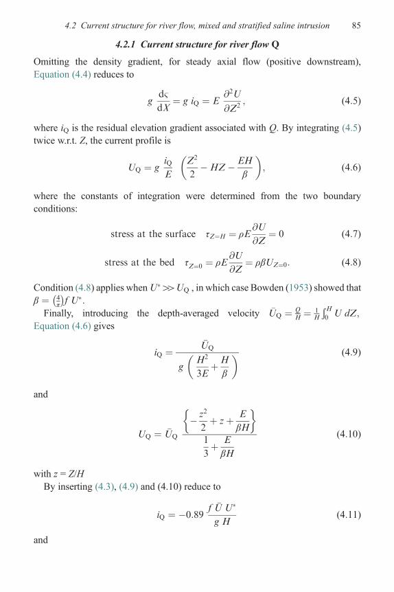
4.2.1 Current structure for river flow Q

Omitting the density gradient, for steady axial flow (positive downstream),Equation (4.4) reduces to

gd&

dX¼ g iQ ¼ E

@2U

@Z2; (4:5)

where iQ is the residual elevation gradient associated with Q. By integrating (4.5)twice w.r.t. Z, the current profile is

UQ ¼ giQE

Z2

2�HZ� EH

β

� �; (4:6)

where the constants of integration were determined from the two boundaryconditions:

stress at the surface τZ¼H ¼ ρE@U

@Z¼ 0 (4:7)

stress at the bed τZ¼0 ¼ ρE@U

@Z¼ ρβUZ¼0: (4:8)

Condition (4.8) applies whenU�44UQ , in which case Bowden (1953) showed thatβ ¼ 4

π

� f U�:

Finally, introducing the depth-averaged velocity �UQ ¼ QH¼ 1

H

ÐH0 U dZ;

Equation (4.6) gives

iQ ¼�UQ

gH2

3EþH

β

� � (4:9)

and

UQ ¼ �UQ

� z2

2þ zþ E

βH

�

1

3þ E

βH

(4:10)

with z = Z/HBy inserting (4.3), (4.9) and (4.10) reduce to

iQ ¼ �0:89f �U U�

g H(4:11)

and

4.2 Current structure for river flow, mixed and stratified saline intrusion 85

UQ ¼ 0:89 �UQ

�z2

2þ zþ π

4

� �: (4:12)

This residual current profile for river flow is illustrated in Fig. 4.4(a) (Prandle, 1985).

4.2.2 Current structure for a well-mixed horizontal density gradient

Again omitting the inertial term before adding a well-mixed longitudinal densitygradient ∂ρ/∂x, the steady state form of (4.4) yields

U ¼ gd&

dX

H2

E

z2

2� z� E

Hβ

� �þ g

ρ@ρ@X

H3

E� z3

6þ z2

2� z

2� E

2Hβ

� �: (4:13)

To isolate the influence of the density gradient, subscript M, we define

d&

dX¼ iQ þ iM: (4:14)

Then subtracting UQ given by (4.10) from (4.13) and applying the condition�UM ¼ 0 and the eddy viscosity formulation (4.3) yields the residual velocitystructure for ‘mixed’ intrusions:

UM ¼ g

ρ@ρ@X

H2

f U U� � z3

6þ 0:269 z2 � 0:037 z� 0:029

� �(4:15)

1.0 1.0 1.0U

Z Z

0.8

0.6

0.4

0.2

0

U / UWU / F SU / F

(c)(b)

Uw Um

(a)

Z

0.80.4 1.2 –0.2 0 0.2 –0.02 0 0.02

Fig. 4.4. Vertical structure for riverine, wind-driven and density-induced residualcurrents. (a) Freshwater flow Q (4.12), point values indicate observed data fromthree positions; (b) wind stress τw (4.37); (c) well-mixed longitudinal densitygradient (4.15). W, F and S defined in (4.42).

86 Saline intrusion

and iM ¼ �0:46H

ρ@ρ@X

: (4:16)

The current profile (4.15) is illustrated in Fig. 4.4(c). The associated net increase inmean sea level over the intrusion length is then approximately 0.013H.

4.2.3 Current structure for a stratified two-layer density regime

Using the notation shown in Fig. 4.5, the pressure at height Z is

in the layer Z � D; p ¼ ρgð& � ZÞ (4:17)

in the bottom layer Z5D; p ¼ ρgð& �DÞ þ ðρþ DρÞg ðD� ZÞ: (4:18)

In addition to the earlier boundary conditions (4.7) and (4.8), we require con-tinuity of both velocity and stress at the interface (subscript I); thus at Z=D,

UI ¼ UB ¼ UT (4:19)

and ρ ET

@UT

@Z¼ ðρþ DρÞ EB

@UB

@Z; (4:20)

where subscripts T and B denote values in the top and bottom layers, respectively.Further assuming:

(a) ρ + Δρ� ρ in mass calculations not involving buoyancy effects,(b) zero net flow in the lower layer, and net flow Q in the top layer,(c) eddy viscosity in the lower layer given by a modified form of (4.3), namely,

EB ¼ fU�dH (4:21)

with d =D/H,(d) eddy viscosity in the top layer given by

ET ¼ γEB: (4:22)

Q

ρ

ρ + ΔρZ

D

H

h

x

ς

Fig. 4.5. Notation for a stratified saline wedge.

4.2 Current structure for river flow, mixed and stratified saline intrusion 87

Then proceeding as in earlier sections, we obtain

UT ¼ �Q"

Hd

1

γz2

2� zþ d� d2

2

� �� 0:308dð1� dÞ

� �(4:23)

UB ¼ �Q"

H

ð1� dÞd2

ð�0:574 z2 þ 0:149 zdþ 0:117d2Þ (4:24)

is ¼ d&

dX¼ �Q" fU�

gH2; (4:25)

where

" ¼ d

ð1� dÞ2 1

3γð1� dÞ þ 0:308d

� � (4:26)

a ¼ 0:149� 1:149d�1 (4:27)

with a ¼Dρρ

dh

dXd&

dX

: (4:28)

From expressions (4.27) and (4.28), the slope of the interface, dh/dX, is alwaysgreater and opposite in sign to the product of surface slope and density difference,(Δρ/ρ dς/dX) except at the surface, d= 1, where they are of equal magnitude.It is difficult to determine a general formulation for γ. Prandle (1985) examined

various possibilities against observed current profiles and suggested the followingexpedient:

γ ¼ 1� d

d: (4:29)

This permits the additional simplifications:

ET ¼ f U�ðH�DÞ (4:30)

iS ¼ �1:56

ð1� dÞ2Q f U�

g H2(4:31)

UT ¼ �1:56Q

H

1

ð1� dÞ3z2

2� z� 0:808d2 þ 1:616d� 0:308

� �(4:32)

UB ¼ �1:56Q

H

1

d2ð1� dÞ �0:574 z2 þ 0:149 zdþ 0:117 d2�

: (4:33)

88 Saline intrusion

4.2.4 Current structure for a constant surface wind stress τw

Proceeding as for net flow Q, but with �UW ¼ 0 and the surface boundary condition

τW ¼ ρE@U

@Z; (4:34)

where τw is an imposed wind stress and subscript W is used to denote wind-drivencomponents, we obtain

UW ¼ τWH

ρE

z2

2

1

2þ E

βH

� �� z

6� 1

6

E

βH

� �

1

3þ E

βH

� � (4:35)

and iW ¼ τWρgH

0:5þ E

βH

� �

1

3þ E

βH

(4:36)

or by introducing (4.3)

UW ¼ τWρfU� 0:574 z2 � 0:149 z� 0:117

� (4:37)

and iw ¼ 1:15τwρgH

: (4:38)

The factor 1.15 in (4.38) lies between the value 1.5 obtained for a no-slip bedcondition and 1.0 for a full-slip condition by Rossiter (1954). The current profile(4.37) is illustrated in Fig. 4.4(b).

4.2.5 Time-averaged vertical salinity structure (mixed)

Scaling analysis can be used to justify the neglect of W ∂C/∂Z in (4.1), andobservations indicate the predominance of the vertical diffusion term. Thence,assuming ∂C/∂X= Sx, omitting time varying terms, we obtain, for Kz constant, thesalinity structure:

sðZÞ ¼ð ð

ρ UMSx

Kz

dZ dZ; (4:39)

i.e. from (4.15), defining vertical variations in salinity as s0(Z) =s(Z) – �S;

s0 ¼ ρgS2

x

EzKz

D5

10 000�83 z5 þ 224 z4 � 62 z3 � 146 z2 þ 33�

: (4:40)

This time-averaged salinity profile is shown in fig. 4.8.

4.2 Current structure for river flow, mixed and stratified saline intrusion 89

4.2.6 Summary

Figure 4.4 shows the residual current profiles (4.12), (4.15) and (4.37) pertaining toriver flow, mixed saline intrusion and wind forcing. Table 4.1 summarises theseresults showing corresponding values at the surface and bed along with relatedgradients in surface elevation.To interpret the magnitudes of these residual flow components, we introduce the

depth-averaged equation of motion for steady state residual flow:

@ζ@X

þ H

2ρ@ρ@X

� τwρgH

þ 4

πfU�U0

gH¼ 0: (4:41)

Then, introducing the dimensionless parameters

S ¼ H@ρρ@X

; W ¼ τWρgH

; F ¼ f U�U0

gH(4:42)

from (4.41), the forcing terms associated with density, wind and bed friction are inthe ratio

S

2: W :

4

πF: (4:43)

FromTable 4.1, the density forcing term S/2 is balanced by a surface gradient – 0.46Swith the remaining component driving a residual circulation of 0.036 SU0/F seawardsat the surface and −0.029 SU0/F (landwards) at the bed. Similarly, the wind stresstermW is counteracted by a surface gradient 1.15Wwith the ‘excess’ balance drivinga circulation of 0.31WU0/F at the surface and −0.12WU0/F at the bed. Clearly, windforcing is more effective in producing a residual circulation than longitudinal densitygradients and both forcings influence elevations to a greater extent than currents.

4.3 The length of saline intrusion

4.3.1 Experimental derivation

Rigter (1973) carried out an extensive study of intrusion lengths both in a laboratoryflume and in the Rotterdam Waterway. The flume was of constant depth andbreadth. Analysis of the experiments resulted in an expression for saline intrusionlength (Prandle, 1985) as follows:

LI ¼ 0:18 g Dρ=ρð ÞD2

f 0 U� U0

¼ 0:005 D2

f U� U0

; (4:44)

where the latter applies for real estuaries with Δρ/ρ� 0.027. Prandle (2004b)indicates that to maintain turbulent Reynolds numbers in flume studies, the friction

90 Saline intrusion

factor must be increased by the same amount as the vertical scale exaggeration,i.e. f 0 = 10f.A comparison of observations from this flume study and computed values for LI

from (4.44) is shown in Fig. 4.6 (Prandle, 1985) for a range of tidal amplitudes, densitydifferences, bed friction coefficients, river flows, water depths and flume lengths. Theexcellent agreement is confirmed by a correlation coefficient calculated as R=0.97,indicating the robustness of (4.44) over a range of parameter sensitivity tests.

4.3.2 Derivations from velocity components

A simple hypothesis for the limit of upstream intrusion is the positionwhere a balanceexists at the bed between (i) the upstream velocity associated with a well-mixedsalinity gradient and (ii) the downstream river velocity. From Table 4.1, this requires

0:029g D2 Sx

f U� ¼ 0:7 U0 (4:45)

i:e: LI ¼ 0:011 D2

f U� U0

; (4:46)

where Sx = 0.027/LI.

0 10

10

20

30

40

50

20LR

LC

30 40 50

Fig. 4.6. Computed versus observed salinity intrusion lengths. Computed, LC (4.44);observed, LR, from flume tests;⊗ reference test, varying: × tidal amplitude,♦ densitydifference,▲ bed friction,★ river flow,■ water depth, + channel length.

4.3 The length of saline intrusion 91

4.3.3 Derivation for a stratified ‘salt wedge’

From integration of the slope of the interface, Prandle (1985) derived the followingexpression for the length of intrusion of a stratified saline wedge

LI ¼ 0:26g D2

f U� U0

Dρρ

¼ 0:07 D2

f U� U0

; (4:47)

where Δρ/ρ� 0.027.This result may be compared with the following expression for the length, LA, of

an arrested saline wedge given by Keulegan (Ippen, 1966, Ch 1):

LA ¼ Ag5=4 D9=4

U5=20

Dρρ

� �5=4

; (4:48)

where A is a parameter which varies with river conditions. Since Keulegan’sexpression was derived from observational data, the correspondence with (4.47)adds useful support to the present theoretical result.Officer (1976, Ch 4) provides alternative derivations for the length of an arrested

salt wedge, the results obtained obviously depend on the particular dynamicalassumptions.

4.3.4 Mean value for saline intrusion length, LI

The above formulations (4.44), (4.46) and (4.47) all show identical expressions forLI but with quantitative values varying by the respective coefficients 0.005, 0.011and 0.07. To reconcile these, we note that the balancing of sea-bed velocity com-ponents in (4.46) should strictly use values of D and U at the landward limit ofthe wedge, resulting in a decrease in the coefficient shown. Likewise, it is widelyobserved that intrusion lengths in stratified conditions are significantly longer thanin mixed. Thus, henceforth we adopt the value (4.44).A subsequent derivation (4.59), based on balancing the mixing rates associated

with the density structure (4.54) with river flow (4.57), provides a further estimatefor LI in close agreement with (4.44).

Observed versus computed values

A major difficulty in assessing the validity of (4.44) is the paucity of accurateobservational data. Practical application of these estimates for saline intrusionslengths are complicated by a wide spectrum of associated response times. Theserange fromminutes for turbulent intensity levels to hours for effective vertical mixing(Section 4.5) and days for estuarine flushing (4.60). Here, we utilise the observationaldata provided by Prandle (1981) from six estuaries (eight data sets) summarised in

92 Saline intrusion

Table 4.2. This data set provides estimates for intrusion length, LI, riverflow, Q, andestuarine bathymetry. Values forD andU0 at the centre of the intrusionwere estimatedfrom power series approximations to breadth (xn) and depth (xm). The values for U*are estimated from (6.9) derived for synchronous estuaries.Figure 4.7 (Prandle, 2004b) shows estimates of LI from (4.44) based on values for

U0, U* and D at successive positions along the estuaries listed in Table 4.2. Thesevalues are summarised in Table 4.3, indicating values of U0, U* and D at thelocations Xc, where the value of LI from (4.44) equals the observed value L0. It isencouraging to note (Table 4.3) that the values of Xc are in reasonable agreementwith the related observational values X0. Values of U0 range from 0.17 to 0.57 cm−1

with the exception of the St. Lawrence where U0 = 1.4 cm−1.

4.3.5 Axial location of saline intrusion

Figure 4.7 also indicates the landward limits of saline intrusion Xu = (Xc – LI/2)/Lcorresponding to successive values of Xc. We note that, with the exception of theHudson and Delaware, the locations of Xc, where observed and computed values ofLI are equal, correspond with or are slightly seawards of maximum values of Xu, i.e.where the landward limit of saline intrusion is a minimum.Adopting this latter result as a criterion to determine the position, xi, where the

saline intrusion will be centred, requires in dimensionless terms, with x=X/L:

@

@xðx� 0:5liÞ ¼ 0; (4:49)

where li = LI/L. Utilising (4.44) and introducing the shallow water approximation,(6.9), for current amplitude in relation to elevation amplitude, ς*,

Table 4.2 Estuarine parameters

n m L(km) LI(km) D(m) B(km) Q(m3 s1) ς*(m)

(A) Hudson 0.7 0.4 248 99 11.6 3.7 99 0.8(B) Potomac 1.0 0.4 184 74 8.4 18 112 0.7(C) Delaware 2.2 0.3 214 43 4.4 28 300 0.6(D) Bristol Ch. 1.7 1.2 138 55 29.3 20 80 4.0(E) Bristol Ch. 138 8500 4.0(F) Thames 2.3 0.7 95 76 12.6 7 480 2.0(G) Thames 38 19 2.0(H) St. Lawrence 1.5 1.9 48 167 74 48 210 1.5

Notes: L estuarine length, LI observed intrusion length; n, m breadth and depth variations(xn, xm), Q river flow, D depth, B breadth and ς* tidal amplitude at the mouth.Source: Prandle, 1981.

4.3 The length of saline intrusion 93

U�2 ¼ &�oð2gDÞ1=21:33f

: (4:50)

Then further assumingQ =U0Di2/tan α, where tan α is the side slope for a triangular

cross section, we obtain

x2i ¼333 Q tan α

D5=20

: (4:51)

1.0(a) (e)

(f)

(g)

(h)

(b)

(c)

(d)

0.5

0.0

–0.5

–1.0

1.0

0.5

0.0

–0.5

–1.0

1.0

0.5

0.0

–0.5

–1.0

1.0

0.5

0.0

–0.5

–1.0

0.0 0.2 0.4 0.6 0.8 1.0

0.0 0.2 0.4 0.6 0.8 1.0

0.0 0.2 0.4 0.6 0.8 1.0

0.0 0.2 0.4 0.6 0.8 1.0

1.0

0.5

0.0

1.0

0.5

0.0

–0.5

–1.00.0 0.2 0.4 0.6 0.8 1.0

1.0

0.5

0.0

1.0

0.5

0.0

–0.5

–1.00.0 0.2 0.4 0.6 0.8 1.0

1.0

0.5

0.0

1.0

0.5

0.0

–0.5

–1.00.0 0.2 0.4 0.6 0.8 1.0

1.0

0.5

0.0

1.0

0.5

0.0

–0.5

–1.00.0 0.2 0.4 0.6 0.8 1.0

1.0

0.5

0.0

1.0

0.5

0.0

1.0

0.5

0.0

1.0

0.5

0.0

Fig. 4.7. Ratio of computed, Lc, to observed, L0, saline intrusion lengths at varyinglocations, Xc. Results for (a) Hudson (b) Potomac (c) Delaware (d) Bristol Channel,Q = 80m3 s−1 (e) Bristol Channel, Q = 480m3 s−1 (f) Thames, Q = 19m3 s−1 (g)Thames, Q= 210m3 s−1 and (h) St. Lawrence. Horizontal axis, XC /L. Point value Xis the centre of observed intrusion. Vertical axis, (LHS) log10 LC/L0, full line, (RHS)landward limit of intrusion; XU= (XC–LI/2)/L, dashed line; LC from (4.44).

94 Saline intrusion

By further introducing the derivation for a synchronous estuary in Chapter 6 thatdepths and breadths vary with x 0.8, the depth, Di at xi is D0xi

0.8 giving a residualvelocity U0 at the centre of the intrusion:

U0 ¼ D1=2i

333m s�1: (4:52)

This expression yields values of U0 = 0.006m s−1 for D = 4m, 0.012m s−1 forD= 16m.Noting that (4.51) corresponds to li = 2/3xi, these values for U0 will increase

by a factor of 2 at the upstream limit and decrease by 40% at the downstreamlimit. Noting also the inaccuracy inherent in measurements of U0, we concludethat these estimates of residual velocity associated with river flow in the salineintrusion region are reasonably consistent with the observed values shown inTable 4.3.If in proceeding from (4.49) to (4.51) we introduce estuarine bathymetry with

breadth B0xn and depth D0x

m, we obtain the following alternative form for (4.51)

xi ¼ 855 Q

D3=20 B0 11m=4þ n� 1ð Þ

!1=ð11m=4Þþn�1

: (4:53)

An especially interesting feature of the results for the axial location of salineintrusion (4.51) and (4.53) and the expression for residual river flow current(4.52) is their independence of both tidal amplitude and bed friction coefficient.(Although there is an implicit requirement that tidal amplitude is sufficient tomaintain partially mixed conditions.) Equations (4.51) and (4.53) emphasise howthe centre of the intrusion adjusts for changes in river flowQ. This ‘axial migration’

Table 4.3 Observed and computed estuarine parameters for saline intrusion

X0 Xc U0 (cm s−1) U* (m s−1) D (m)

(A) Hudson 0.80 0.70 0.35 0.59 9.7(B) Potomac 0.60 0.50 0.20 0.54 6.3(C) Delaware 0.80 1.0 0.29 0.47 4.4(D) Bristol Ch. 0.30 0.40 0.22 1.53 9.5(E) Bristol Ch. 0.55 0.65 0.28 1.70 17.3(F) Thames 0.60 0.55 0.17 1.01 8.0(G) Thames 0.75 0.50 0.57 1.06 10.2(H) St. Lawrence 0.60 0.65 1.4 0.80 30.0

Notes: X0 (fraction of L) centre of observed intrusion, Xc centre of intrusion whenLI (4.44) = L0, observed; D, U0 =Q/area, U* depth, residual and tidal currents at Xc.Source: Prandle, 2004a.

4.3 The length of saline intrusion 95

can severely complicate the sensitivity of saline intrusion beyond the anticipateddirect responses apparent from the expression (4.44) for the length of intrusion, LI.

4.4 Tidal straining and convective overturning

The preceding studies, involving tidally averaged linearised theories relating to thevertical structure of salinity and velocities, are now extended by numerical simula-tions incorporating tidal straining and associated convective overturning.

4.4.1 Rates of mixing

Before describing the modelling study, we first examine rates of mixing associatedwith (i) time-averaged density structure, (ii) tidal straining and (iii) supply of fresh-water velocity.From (4.1), the mean rate of mixing MK associated with the

time-averaged density structure (4.40) is (Simpson et al., 1990)

MK ¼ ρðD

0

@

@ZKz

@s

@Z

�������� dZ ¼ 0:02ρg

S2xD

4

E: (4:54)

Themean rate of overturning to compensate for tidal straining on the flood phaseM0 is

M0 ¼ ρ2

πU� Sx D

ð1

0

0:7þ 0:9z� 0:45z2 � 1�

dz�� (4:55)

¼ 0:12ρSxDU�; (4:56)

where the approximation for the vertical structure of tidal currents is similar to thatof Bowden and Fairbairn (1952). Nunes Vaz and Simpson (1994) derive additionalcontributions to vertical mixing associated with wind, surface heat exchange andevapo-transpiration.For a stationary salinity distribution, the mixing rate MQ to balance freshwater

velocity U0 is

MQ ¼ ρU0SxD: (4:57)

Then to balance MQ, we expect values of U0 of

tidal straining on flood tide 0:12U� (4:58)

vertical salinity difference 0:02gSxD

3

E: (4:59)

96 Saline intrusion

For U* = 0.5m s−1, assuming no mixing on the ebb tide, (4.58) indicates a valueof U0 = 3 cm s−1. Since this value generally exceeds that associated with verticalsalinity differences (4.59), we expect that tidal straining will often eliminate verticalsalinity differences by the end of the flood tide, see Fig. 4.10. Equation (4.59)provides an expression for saline intrusion length LI almost identical to (4.44).For a prismatic channel, the estuarine flushing time, TF can be approximated

by the time taken to replace half of the fresh water in the intrusion zone by riverflow, i.e.

TF ¼ 0:5ðLI=2ÞU0

: (4:60)

For typical values of TF = 2–10 days, this requires U0 varying from 1.5 to 3 cm s−1

over the range of intrusion lengths LI = 12.5 to 100 km considered in Figs 4.11and 4.12.

4.4.2 Modelling approach (Prandle, 2004a)

The significance of tidal straining is evaluated by reference to a ‘single-point’numerical model in which the time-varying cycle of depth-averaged tidal currentamplitude, U*, and a (temporally and vertically) constant saline gradient, Sx, arespecified (Prandle, 2004a). The model illustrates the role of convective overturningin counteracting unstable density structures introduced by tidal straining. Thevalidity of the model is evaluated by simulation of measurements by Rippethet al. (2001).To explore the generality of estuarine responses, the model is run for a wide range

of values of saline intrusion lengths, LI , and water depths,D. Additional sensitivityanalyses are made for changes in U* and the bed stress coefficient, f. The model isused to calculate the following parameters: surface-to-bed differences in bothresidual velocity, δu, and salinity, δs; the potential energy anomaly �M (4.65); theratio of mixing by diffusivity: overturning; the efficiency of mixing ε and the riverflow U0 (required to balance mixing rates). Thus, the model simulations illustrate,over a wide range of estuarine conditions, the impact of tidal straining and, thereby,the significance of its omission in the analytical formulations.

4.4.3 Model formulation

We assume (vertically and temporally) constant coefficients for eddy viscosity anddiffusivity; however, a partial assessment of buoyancymodulation of eddy viscosityand diffusivity is examined by introducing the formulations of Munk and Anderson(1948):

4.4 Tidal straining and convective overturning 97

eddy viscosity Ez ¼ f U� D ð1þ 10RiÞ�1=2 (4:61)

eddy diffusivity Kz ¼ f U� D=Sc ð1þ 3:33RiÞ�3=2; (4:62)

where the Richardson number, Ri, is given by (4.2) and Sc is the Schmidt numberrepresenting the ratio E :Kz. Nunes Vaz and Simpson (1994) describe a wide rangeof such formulations.A single-point numerical model was formulated providing solutions to (4.1) and

(4.4). The model is forced via specification of the depth-averaged semi-diurnaltidal current amplitude, U*, and the (temporally and vertically constant) salinitygradient, Sx. The model was run for a (small) number of tidal cycles to achievecyclic convergence.Boundary conditions were specified as zero stress at the surface and bed

stress

τZ ¼ ρ f U2z¼ 0: (4:63)

The model incorporates convective overturning whenever density decreases withdepth.To distinguish the effect of (i) buoyancy modulation of E and Kz (via (4.61) and

(4.62)) and (ii) convective overturning, three separate simulationsweremade. The firstsimulation used constant values of E= fU*D andKz = ScE. The second modified thesevalues according to (4.61) and (4.62) and the third introduced convective overturning(in addition to (4.61) and (4.62)). Results from the first two simulations showed littledifference, except for applications involving pronounced stratificationwhere (4.1) and(4.4) become invalid. Hence, results are only shown for (i) Simulation 1 whereE= fU*D, Kz = ScE without convective overturning and (ii) Simulation 3 with E andKz from (4.61) and (4.62) and convective overturning included.

4.4.4 Model results

Currents

Figure 4.8(a) shows tidally averaged (residual) current profiles obtained fromSimulations 1 and 3 together with the theoretical profile (4.15). The parameters,U* = 0.6m s−1 f= 0.0025, D= 32m, L= 400 km, Sc = 0.1, were used to correspondto the observations by Rippeth et al. (2001). Without overturning, the modelaccurately reproduced the earlier theoretical vertical profiles of both tidal currentamplitude and phase. The results for model Simulation 1 and the theoretical solution(4.15) are near-identical. By contrast, the results for Simulation 3 show similarprofiles but with the magnitude doubled.

98 Saline intrusion

Sensitivity analyses of Simulation 3 showed little variation with changes in theSchmid number. However, doubling U* produces a one-third reduction in residualvelocities while quadrupling f produces a two-third reduction.

Salinity

Figure 4.8 (Prandle, 2004a) shows tidally averaged salinity profiles (converted topsu) for these same simulations compared with the theoretical profile from (4.40).Again, the theoretical result is near-identical to Simulation 1. However, Simulation3 shows results four times larger with a net surface-to-bed value of δs= 0.25‰similar to the observed values indicated by Rippeth et al. (2001).Figure 4.9 (Prandle, 2004a) shows a tidal cycle of dissipation due to (i) bottom

friction ρfU3/D and (ii) depth-averaged vertical shear ρE(∂U/∂Z)2. The former

1.0

0.8

0.6

0.4

0.2

0.0–0.04 –0.02 0.00 0.02 0.04

1.0

0.8

0.6

0.4

0.2

0.0–0.15 –0.075 0.0 0.075 0.15

1.0

0.8

0.6

0.4

0.2

0.0–0.15 –0.075 0.0 0.075 0.15

1.0

0.8

0.6

0.4

0.2

0.0–0.04 –0.02 0.00 0.02 0.04

(b)

(a)

Fig. 4.8. Vertical profiles of (a) residual velocity (4.15), m s−1, and (b) salinitydifferences (4.40),‰. Left: dashed lines, theory; full lines, numerical model; thin,Simulation 1; thick, Simulation 3. Right: Simulation 3 with thin, f = 0.01; dashed,U* = 1.2m s−1; thick Sc = 1. Values correspond to U* = 0.6m s−1, f = 0.0025,D = 32m, L = 400 km, Sc = 10.

4.4 Tidal straining and convective overturning 99

shows a pattern directly linked to tidal current speed. The vertical shear shows peakvalues on the decelerating phases of both ebb and flood flows but with markedlystronger values on the ebb. Interestingly, the peak values of dissipation, order of (2 ×10−2Wm−3), are similar for both values of the Sc= 10 and 1. Rippeth et al. indicatedcomparable rates of dissipation up to 0.5 × 10−2Wm−3.

Tidal cycle and depth profiles

Figure 4.10 (Prandle, 2004a) shows that tidal cycles of vertical differences forsalinity for the Simulation 3 runs with Sc = 10 and 1.0. For Sc = 1.0, completevertical mixing, due to convective overturning, is shown to start about 1.5 h after thestart of the flood tide and to continue for about one-third of the cycle. Conversely,for Sc = 10, convective overturning only occurs at the end of the flood tide and islimited in extent to near-bed and near-surface.

4.4.5 Model applications for a range of estuarine conditions

Following the above formulation and evaluation of the single-point model, a rangeof simulations were completed corresponding to

depths D = 4, 5.7, 8, 11.3, 16, 22.6, 32, 45.3, 64mdensity gradients Sx= (Δρ/ρ)/LI, LI = 12.5, 17.7, 25, 35.5, 50, 70.7, 100, 141.4, 200kmtidal velocity U* = 0.5, bed friction f = 0.0025, Schmid number Sc = 10

5 × 10–6

4 × 10–6

3 × 10–6

2 × 10–6

1 × 10–6

0

0.025

0.020

0.015

0.010

0.005

0.000

π 2πMaxflood

Maxebb

0

π 2πMaxflood

Maxebb

0

Fig. 4.9. Tidal cycles of mixing and dissipation rates. Top: depth-averaged mixingrates (kg m−3 s−1). Thin, diffusion Sc = 0.1; dashed, diffusion Sc = 1; thick,overturning. Bottom: dissipation rates (Wm−3). Full, internal shear, dashed, bedfriction; thin Sc = 1.0, thick Sc = 10.

100 Saline intrusion

Δρ= 0.027ρ is ocean salinity and LI the length of saline intrusion. Simulationswere limited to conditions where the bed-to-surface salinity difference, δs, estimatedfrom (4.40) was less than 10‰. Prandle (2004a) provides full details of these modelsimulations.

Tidal velocities

Figure 3.3 indicates the form of the solution (3.16) for tidal current profiles. Thedifference in amplitude between surface and bed increases monotonically withlarger values of the Strouhal number (SR =U*P/D), approaching an asymptoteclose to SR = 350. Since Strouhal numbers in almost all meso- and macro-tidalestuaries will be well in excess of this value, the effects of tidal straining are likelyto be broadly similar across a wide range of such estuaries. In simulations extendingfrom SR = 200 to 10 000, the present applications show a close fit between theory

–40

–20

20

0

0

1.0

0.8

0.6

0.4

0.2

0.00 Max

ebbπ 2πMax

flood

1.0

0.8 –120–80

–100

–60–2020

60

60

–140–120

–100

–80–40

040

80100120

140160

80100

120

0.6

0.4

0.2

0.00 Max

ebbπ 2πMax

flood

Fig. 4.10. Depth profiles of salinity differences over a tidal cycle. Top Sc = 10,bottom Sc = 1.0; contours 0.1‰.

4.4 Tidal straining and convective overturning 101

andmodel for both amplitude and phase of tidal currents. Moreover, these results forvertical profiles of tidal current amplitude and phase are largely insensitive tosalinity gradients over the range considered. Hence, further consideration of tidalcurrents is omitted.Souza and Simpson (1997) used H.F. Radar observations of surface tidal ellipses

in a coastal (freshwater) plume region to indicate how a two-layer tidal responsecan develop. In the limit, the surface layer response is effectively frictionless, andthe lower layer responds like a water column reduced in depth to that at theirinterface. While such results may be encountered in estuaries with weak tides, theassociated dynamics involve convective and Coriolis terms omitted from (4.4).

Bed-to-surface residual current differences δuand sea level gradient ∂ς /∂X

Figure 4.11(a) (Prandle, 2004a) shows the values of δu, the bed-to-surface differencein tidally averaged velocities derived from (4.15) and Simulations 1 and 3 (using themodel described in Section 4.4.3). The figure indicates values of δu throughout therange of both intrusion lengths, LI, and water depths, D, noted above. The resultsshown are forU* = 0.5m s−1, f = 0.0025 and Sc = 10. The dots in Figs 4.11 and 4.12represent values of (D, LI) from the eight observational data sets listed in Tables 4.2and 4.3.The use of axes with scales based on log2(200/LI) and log2(D/4) results in contour

distributions with slope a= n/m for a parameter dependent on LImDn. Thus,

for (4.15), where δu∝D2/LI fU*, the slope is − 2 and the spacing is log2 R1/n on

the D-axis and log2 R1/m on the LI axis, where R is the ratio between contour values.

12.5(a) (b)

25

L 1 (k

m)

50

100

2004 8

1

55

10.1

16D (m)

32 64

12.5

25

L 1 (k

m)

50

100

2004 8

0.1

1.01.0

10

0.010.1

16D (m)

32 64

Û = 0.5 m s–1

Sc = 10k = 0.0025

Û = 0.5 m s–1

Sc = 10

ν = 1

ν = 0

k = 0.0025

Fig. 4.11. Bed to surface changes as f (depth, D, and saline intrusion length, LI).(a) residual velocity (cm s−1), (b) salinity (‰). Dashed lines, numerical model, fulllines, theory (4.15) and (4.40). Dots indicate observed values (Prandle, 2004b).Shaded area in (b) indicates 0 < υ < 1, where υ (Hansen and Rattray, 1966), is theratio of salt flux associated with vertical diffusion to that due to gravitationalconvection.

102 Saline intrusion

The values of δu from Simulation 1 (E = f U*D, no overturning) are in closeagreement with the derived expression (4.15), as indicated previously. However, theintroduction of overturning into Simulation 3 significantly enhances values of δurelative to (4.15) while maintaining the theoretical dependence on D2/LI.Associated results for the magnitude of the tidally averaged sea surface gradient

∂ς/∂X from both Simulations 1 and 3 are in precise agreement with the derivedvalues from (4.16). Over the ranges of D and LI considered, ∂ς/∂X is shown toincrease up to 10× 10−6 which corresponds to a net increase in sea level of 1 cmkm−1

of intrusion length.

Bed-to-surface density differences, δs

Figure 4.11(b) shows values of δs, the tidally averaged bed-to-surface differencein salinity. Again, results from Simulation 1 (without overturning) are in closeagreement with the derived expression from (4.40), maintaining the dependencyon D3/LI

2.

12.5

25

L 1 (k

m)

50

1

0.1

0.110

1

10

0.015

0.005

0.001

100

2004 8 16

D (m)32 64

12.5

25

L 1 (k

m)

50

100

200

0.4

0.25

0.1

Mixingoverturning:dispersion

Uo cm s–1

Φ j m–3 ε

2.5

0.12.0

1.5

1.0

4 8 16D (m)

32 64

12.5

25

L 1 (k

m)

50

100

2004 8 16

D (m)32 64

12.5

25

L 1 (k

m)

50

100

2004 8 16

D (m)32 64

Fig. 4.12. Potential energy anomaly, φM; mixing efficiency, ε; overturning:diffusivity; river flow. Contours as for Fig. 4.11.(Top left) Tidal mean potential energy anomaly φM, (4.64), in Jm−3.(Top right) Efficiency of mixing, ε.(Bottom left)Tidalmean ratioofmixingbyconvectiveoverturning : vertical diffusivity.(Bottom right) Balancing river flows,U0 (cm s−1).

4.4 Tidal straining and convective overturning 103

However, as previously indicated in Fig. 4.8, results from Simulation 3 (withoverturning) are radically different with enhanced values of δs. Moreover, thesecontours suggest a dependency onD/LI. The tidal cycles shown in Fig. 4.10 indicatehow overturning eliminates the balancing of ebb–flood tidal straining maintainedin Simulation 1.

4.4.6 Mixing processes

The potential energy anomaly φE, is defined as

φE ¼ 1

D

ðD

0

s0gðZ�DÞdZ; (4:64)

where s0 is determined from the tidal current structure indicated in (4.40).This represents the amount of energy required to mix the water column to a

uniform density and hence, inversely, the effectiveness of vertical mixing.Substituting (4.40) in (4.64), we obtain a time-averaged value of φE associated

with the tidally averaged density structure:

�M ¼ 0:0007ρg2S2xD

6

EKz

: (4:65)

The tidally averaged results for φM shown in Fig. 4.12 correspond to the densitydifferences described in the previous section. For Simulation 1, without overturn-ing, calculated values of φM (not shown) are in close correspondence with (4.65)maintaining a dependency on D2/LI. Whereas, for Simulation 3 with overturning,radically enhanced values of φM are obtained with a dependency closer to D5/3/LI.Typically, larger values of φE are found over much of the tidal cycle, but these arereduced to zero by overturning over as much as one-third of the tidal cycle.Details of the separate mixing processes within the simulations can be quanti-

fied. Figure 4.12 (Prandle, 2004a) shows, for Simulation 3, the ratio of (tidallyaveraged) mixing by convective overturning to that by vertical diffusivity. Themaximum value of this ratio is 0.4 and occurs in shallow water for large values ofLI. This ratio decreases to 0.1 in deeper more stratified conditions.The effectiveness of mixing, ε, is defined by Simpson and Bowers (1981) as the

ratio of work done by mixing to that by tidal friction at the bed. Figure 4.12 shows,for Simulation 3, values of ε ranging from less than 0.001 in well-mixed condi-tions up to 0.015 in more stratified conditions. Here, the total work done includesboth that by bed friction (ρfU3

bed) and that by internal shear ∫ρEz(dU/dZ)2 dZ.

Interestingly, the Simpson and Bowers (1981) estimate of ε ≈ 0.004 lies closeto the centre of the calculated distributions. Hearn (1985) noted the ubiquity of

104 Saline intrusion

ε� 0.003 in shelf seas. He also shows values of ε ranging from 0.003 to 0.016based on observations at three sites (90–100m deep) in the Celtic Sea.Figure 4.12 also shows the value of U0 required to balance the total rate of

mixing. In Simulation 3, these values range from a maximum of 2.5 cm s−1 inshallow water to 1.5 cm s−1 in deeper water. A value of 3 cm s−1 is suggestedfrom (4.58) due to tidally averaged tidal straining and between 0.1 and 1.0 cm s−1

from (4.59) due to vertical density differences. The latter values are closer totypical observed values shown in Tables 4.2 and 4.3 and suggest that somerelaxation of constant Sx may occur that reduces mixing associated with tidalstraining.

4.5 Stratification

4.5.1 Flow ratio, FR

It is generally accepted that stratification strengthens with increased values ofdepth D and river flow Q and with decreased values of breadth B and tidal currentamplitude U*. The flow ratio, FR, is defined as the net freshwater flow over a tidalcycle divided by the tidal prism, TP, entering the estuary each flood tide, i.e.approximately the volume between high and low waters:

FR ¼ QP

TP

� QπU�BD

¼ U0πU� : (4:66)

The above assumes that TP can be approximated by U* A P/π, where A=BD is thecross-sectional area. Schultz and Simmons (1957) suggested that estuaries arewell-mixed for FR < 0.1, i.e. U0 < 0.03 U*.The parameter dependencies in (4.66) confirm the tendencies towards stratifica-

tion noted above – with the exception of the influence of depth D. The followingsection explains this anomaly, illustrating how the kinetic relationship (4.66) needsto be extended to consider the balance between the rate of mixing (often concen-trated near the surface in stratified flow) and the tidal dissipation (concentratedclose to the bed). Chapter 3 shows that for (ωD/fU*) > 0.25, i.e. D/U* > 5 s for asemi-diurnal tide, maximum velocities occur around mid-depth, with little currentshear in the top half of the water. Subsequent sections confirm that, except fordeeper micro-tidal estuaries where mixing scarcely extends to the surface, (4.66) isthe primary indicator of stratification.

4.5.2 Energy and time requirements

The Simpson–Hunter (1974) criteria for stratified conditions is based on the ratiobetween the increase in potential energy due to mixing and the associated work

4.5 Stratification 105

done by tidal friction. The quantitative value indicative of mixing throughout thedepth,

H=U�3555 m2 s3; (4:67)

is based on observational evidence of thermal stratification in shelf seas.Prandle (1997) indicated that stratification levels can be calculated from the time,

D2/Kz, for complete vertical mixing by diffusion of a point source introduced at thesurface or bed. Inserting (4.3) and specifying the time limit as the duration of the ebbor flood phases, stratification requires

D2

Kz

¼ D

Sc f U�46 h or

D

U� 456 Sc s: (4:68)

SinceU* is usually in the range 0.5–1.0m s−1, and Sc between 0.1 and 1, we see thecorrespondence with the Simpson–Hunter criterion. Most estuaries have values ofD2/Kz > 1 h, indicating that some degree of intra-tidal stratification will occur. InChapter 6, it is shown how, for a synchronous estuary, both criteria correspondclosely to stratification occurring for tidal elevation amplitudes ς* ≤ 1m.

4.5.3 Richardson number

Time- and depth-averaged values for Ri (4.2) can be calculated using (4.40) for∂ρ/∂Z and (4.55) for ∂U/∂Z, giving

Ri ¼68gS2

x D4

104 E Kz

0:45U�

D

� �2¼ 100Sc

U0

U�

� �2

: (4:69)

Thus, with E from (4.3), Sx = 0.027/LI, where LI is the saline intrusion length from(4.44). The condition, Ri < 0.25, for mixing to occur, corresponds to U0 < 0.05 U*for Sc = 1 and U0 < 0.016 U* for Sc = 10.

4.5.4 Stratification number

Ippen and Harleman (1961) demonstrated that vertical mixing could be relatedto the balance between turbulence associated with the rate of dissipation of tidalenergy by bed stress, G = ε(4/3π)fρU*3LI, and the energy required to increasethe potential energy level by vertical mixing, J =½ Δρ g H2U0. The parameter εrepresenting the efficiency of mixing, typically �0.004 (Section 4.4.6), is intro-duced here to give a modified stratification number, defined as

106 Saline intrusion

S0T ¼ ST" ¼ "G

J¼ 0:85

" f U�LI

�ρρ gH2U0

¼ 0:017 "U�

U0

� �2

: (4:70)

Thus, the stratification number extends the concept of the Simpson–Hunter criteriondescribed in Section 4.5.2 to balance net mixing of fresh water input over the salineintrusion length. Prandle (1985) showed that estuaries change from mixed to strati-fied as the stratification number decreases from above 400 to below 100 (Fig. 4.13;Prandle, 1985). Adopting the limit ST = 250, then for ε= 0.004, the boundary corre-sponds to ST

` = 1 and U0 < 0.01 U*.

4.5.5 Vertical salinity difference

Hansen and Rattray (1966) indicated that a normalised surface to bed salinitydifferences of δs/s < 0.1 could be adopted as the boundary for mixed and stratifiedestuaries. From Fig. 4.13 and (4.70),

δss¼ 4S�0:5

T ¼ 31U0

U�

� �: (4:71)

Thus, δs/s < 0.1 implies that estuaries will be mixed for U0 < 0.003 U*. Using thesuggested revised demarcation, based on Fig. 4.13, of ST = 250, stratification isdefined as δs/s > 0.25, U0 > 0.01 U*.

10

5

2

1.0

0.1

0.011 2 5 10 100

St

1000 10000

Well-mixedStratified

δs/s

Fig. 4.13. Level of stratification δs/s versus Stratification number ST. ST = 0.017ε (U*/U0)

2, (4.70). • Rigter’s (1973) flume tests, + WES flume tests, ×observations.

4.5 Stratification 107

4.6 Summary of results and guidelines for application

Within estuaries, saline intrusion can impact significantly on flora, fauna, biology,chemistry, sediments, morphology, flushing time, contaminant pathways, etc. Herewe examine the dynamics of mixing, indicating how bathymetry and both marineand fluvial conditions determine the degree of stratification and the extent of axialpenetration. Appendix 4A outlines the characteristics of the related dependency ofwater density on temperature, illustrating how the seasonal cycle varies according tothe level of stratification and latitude.The leading question is:

How does salt water intrude and mix and how does this change over cycles ofspring–neap tides and flood-to-drought river flows?

Apart from an occasional surface scum line, the ebb and flood of saline intrusionin estuaries passes largely unnoticed. Yet, the extent of saline intrusion was often thedetermining factor in the siting of towns or industries reliant on fresh river water.Moreover, the extent and nature of intrusions determines net estuarine concentra-tions of both dissolvedmarine tracers and fluvial contaminants. At the interface withriver water, salt water produces electrolytic attraction between fine suspendedsediments resulting in rapidly settling ‘flocs’ which accumulate at the seaward(ebb) and landward (flood) limits of intrusion.In strongly tidal estuaries, saline intrusion has little impact on tidal propagation

(Prandle, 2004a). Conversely, the nature of saline intrusion is overwhelminglydetermined by the combination of tidal motions alongside the flow of river water.Pritchard (1955) introduced a generalised classification of estuaries according totheir salinity intrusion, varying from fully mixed (vertically) in strongly tidal,shallow estuaries with small river flows through to ‘arrested saline wedge’ in deeper,micro-tidal estuaries with large river flows. Hansen and Rattray (1966) produced ageneralised stratification diagram (Fig. 4.3), converted by Prandle (1985) in terms ofmore readily available parameters. However, this diagram does not directly answerthe above question concerning the range of saline intrusion in estuaries.Stratification is complicated by continuous interactions between the dynamics

promoting mixing and associated adjustments to the background salinity gradients.The Richardson number (4.2), quantifies the ratio of ‘stabilising’ buoyancy inflow tothe rate of turbulent mixing. It has proven a robust indicator of stratification across awide range of fluid dynamics.However, this number can vary appreciably over the tidaland fluvial cycles noted above and frommouth to head and laterally within an estuary.Section 4.3 describes how various approaches for estimating the length of saline

intrusion, LI, all suggest a dependence on D2/f U*U0 (D depth f bed frictioncoefficient, U* tidal current amplitude and U0 residual current associated with

108 Saline intrusion

river flow). Assessments against a range of flume tests indicate the validity androbustness of this formulation. However, this formula fails to account for observedvariations in intrusion lengths (Uncles et al., 2002). The additional factor, whichmust be incorporated in funnel-shaped estuaries, is axial migration of the intrusion.This introduces a complex inter-dependency between the length and the location ofthe intrusion. Analysis of observations suggests that this axial migration adjusts toenable mixing to occur as far seawards as is consistent with containing the mixingwithin the estuary. The time delay for such axial migration of the intrusion is relatedto the estuarine flushing time TF. It is shown in Chapter 6 and from observationsthat TF is in the range of days, and hence changing tidal and river flow conditionsover such periods further complicates the calculation of LI. Clearly, model sim-ulations need to extend adequately in time to accommodate such migrations andincorporate appropriate ‘relaxation’ of both seaward and landward boundaryconditions.Abraham (1988) noted the significance of ‘tidal straining’, whereby on the flood

tide, larger near-surface tidal velocities advect denser more saline water over fresherlower layers leading to mixing by convective overturning. Simpson et al. (1990)provided both theoretical and observational quantification of this phenomenon.However, despite the neglect of this latter effect, ‘tidally averaged’ analyticalsolutions for salinity-induced vertical profiles of residual velocities and salinitiesare found to be widely applicable. The summary of these analytical solutions inSection 4.2.6 and Table 4.1 emphasises how, for steady-state equilibria, the dyna-mical adjustments to saline intrusion involve small (relative to tidal components),residual currents and surface gradients.These solutions provide estimates for residual flow components associated with

(i) river flow Q (4.12), (ii) wind stress τw (4.37), (iii) a well-mixed longitudinaldensity gradient (4.15), and (iv) a fully stratified saline wedge (4.32) and (4.33).The relative magnitudes of each of these components are defined in terms ofdimensionless parameters (4.42). The residual current profiles (i), (ii) and (iii) areshown in Fig. 4.4.From Table 4.1, the density forcing term 0.5S is balanced by a surface gradi-

ent −0.46S with the remaining component driving a residual circulation of 0.036SU0/F seawards at the surface and −0.029S U0/F (landwards) at the bed. Similarly,the wind stress term −W is counteracted by a surface gradient 1.15W with the‘excess’ balance driving a circulation of 0.31W U0/F at the surface and −0.12WU0/F at the bed (W, S and F are defined in (4.42)). Thus, for steady-stateconditions, both wind and density forcing are mainly balanced by surface gradi-ents with only a small fraction of the forcing effective in maintaining a verticalcirculation.

4.6 Summary of results and guidelines for application 109

Section 4.4 uses these analytically derived current and salinity profiles to estimatethe (localised) rates of vertical mixing and compares these alongside the valuesassociated with tidal straining to the rate of supply of river water. These analyticalsolutions are further compared with results from a ‘single-point’ numerical modelwhich incorporates tidal straining and convective overturning whenever densitydecreases with depth. The model also includes the Munk and Anderson (1948)modifications of the eddy diffusivity and eddy viscosity coefficients, E and Kz,based on Richardson number representations of buoyancy effects.The application of this numerical model extends to a range of values of both

intrusion lengths, LI , and water depths, D. Sensitivities to the Schmidt number,expressing the ratio of E:Kz are also explored. Results are shown for surface-to-bed differences in residual velocity, δu, and salinity, δs; potential energy anomaly,φE; the ratio of mixing by diffusivity: overturning; the efficiency of mixing ε andresidual river flow U0 (required to balance mixing rates).Qualitatively, both numerical model and analytical solutions for the residual

currents and salinity profiles are in close agreement. However, the model sug-gests that tidal straining can increase the magnitudes of these currents and salinitystructure several fold. Averaged over a tidal cycle, the component of mixingassociated with overturning is shown to be generally significantly less than mixingby diffusion, typically 0.1−0.4 of the latter. However, the pronounced impact ofoverturning in removing stratification on the flood tide is evident. The model alsoquantifies mixing rates related to bed friction and internal shear. The resultsconfirm Simpson and Bower’s (1981) observational findings that less than 1%of the energy involved in tidal dissipation is effective in promoting vertical mixing.Section 4.5 revisits the issue of indicators for estuarine stratification. New

theories on stratification are reconciled with historical indicators, emphasising thatU0/U* > 0.01 is the common key indicator of stratification. Calculations are made oflikely values ofU0 in the saline intrusion zone based on (i) most seaward location ofmixing (4.52); (ii) a flow ratio, FR =U0 π/U* = 0.1 (4.66); (iii) a Richardson numberRI = 0.25 (4.69); (iv) a balance between gain in potential energy and tidal dissipation(4.70); and (v) observations of stratification (Fig. 4.13). All five approaches indicatevalues of U0 close to 1 cm s−1 in the intrusion zone of ‘mixed’ estuaries – a resultsubsequently further confirmed in Chapter 6. This indicator confirms that stratifica-tion generally increases with larger river flow, narrower breadths and weaker tidalcurrents. However, the indication that stratification increases with shallower water iscounteracted by reduced tidal current shear nearer the surface in deep water and therelated reduced role of tidal straining.Appendix 4A provides expressions for the mean and seasonal variations of both

the water surface and the ambient air as functions of depth, latitude and degree ofstratification.

110 Saline intrusion

Appendix 4A

4A.1 The annual temperature cycle

A generalised theory is developed to describe the annual temperature cycle inestuaries and adjacent seas. A sinusoidal approximation to the annual solar heatingcomponent, S, is assumed and the surface loss term is expressed as a constant, k,times the air-sea temperature difference (Ta – Ts). For vertically mixed conditions,analytical solutions show that in shallow depths, the water temperature followsclosely that of the ambient air temperature with limited separate effect of solarheating. Conversely in greater depths, the water surface temperature variations willbe reduced relative to those of the ambient air. Providing such deep water remainsmixed vertically, the seasonal variation will be inversely proportional to depth andmaximum temperatureswill occur up to 3months after themaximumof solar heating.The annual mean water temperature will exceed the annual mean air temperature bythe annual mean of S divided by k. For wider applications, a numerical model is usedto derive generalised expressions for the mean and amplitude of both air and watersurface temperatures as functions of latitude, depth and tidal current speed.The description of temperature in marine ecological models is important both

directly for its influence on specific parameters and indirectly via its contribution tovertical density variations.Water density can be approximated by ρ=1000 + 0.7S – 0.2 T (kgm−3), where S is

salinity in‰ and T is temperature in °C. Thus, stratification at the demarcation limit,δS� 0.25‰, is equivalent to a surface-to-bed temperature difference of 0.875 °C .Simplified and generalised approaches are used to examine how the seasonal

temperatures vary with (i) the level of solar heating (i.e. cloud cover and latitude), (ii)ambient air temperature, (iii) wind speed (strongly controlling the rate of air-sea heatexchange), (iv) water depth and (v) the degree of vertical stirring. Results from thesesstudies (Prandle and Lane, 1995; Prandle, 1998) can be used to examine the impact ofchanges in any of these parameters that might arise from climate trends, etc.The fundamental simplifications introduced are as follows:

(1) approximation of the annual solar heat input by a mean value plus a sinusoidal term:S0 – S* cosωt;

(2) representation of the heat losses by a term k(Ts – Ta), where Ts is the water surfacetemperature, Ta the air temperature and k a constant coefficient;

(3) assumption of a localised equilibrium, i.e. neglect of horizontal components of advec-tion and dispersion;

(4) representation of vertical mixing processes by an eddy dispersion coefficient encom-passing the effects of vertical mixing processes by both vertical advection and dispersion;

(5) neglect of both the (solar) diurnal and the neap–spring tidal cycles of variability.

Appendix 4A 111

The adoption of a sinusoidal approximation to the annual temperature cycleinvolves phase values with 360° corresponding to 1 year. For convenience, the‘year’ is here shortened to 360 days so that 1° corresponds to 1 day. Where ‘daynumbers’ are cited, strictly, these start at the winter solstice.

4A.2 Components of heat exchange at the sea surface

Goldsmith andBunker (1979) describe four components involved in the heat exchangebetween the atmosphere and the sea, namely

(1) SR – solar radiation, i.e. the primary energy source;(2) LH – latent heat flux, heat lost from the sea by evaporation (occasionally gained by

condensation);(3) IR – infrared back radiation, the net effective ‘reflection’ from the sea;(4) LS – sensible heat flux, heat exchange between air and sea by ‘conduction’.

Figure 4A.1 shows the annual variation of SR, LH, IR and LS at 55°N, 3°E (northernNorth Sea) based on data for 1989 supplied by the UK.Meteorological Office, Cave(1990) and heat exchange terms calculated fromGoldsmith and Bunker (1979). Theeffective value of SR at the sea surface is reduced by cloud cover, this reduction isabout 1/8 for 25% cover, 1/3 for 50% cover and 4/5 for 100% cover. However, theannual cycle (frequency ω) at almost all latitudes can be approximated by

SR ¼ Sð1� β cosotÞ: (4A:1)

The latent heat flux LH is a function of wind speed W, the air–sea temperaturedifference (Ta – Ts) and relative humidity.The effective back radiation IR depends on the absorptive properties of the

atmosphere and both Ta and Ts; however, it is most sensitive to Ta.The sensible heat flux LS is proportional to both wind speedW and (Ts – Ta). Air

gains heat quicker than water as a consequence of their relative thermal conductiv-ities, i.e. 0.0226 and 0.60Wm−1 °C−1, respectively, and hence the assumption of aconstant value for k may be invalid in seas where Ta > Ts for extended periods.For simplicity, we lump together solar radiation SR and infrared back radiation

IR into a single heat gain term S approximated by

SðtÞ ¼ S0 � S� cosot: (4A:2)

Likewise, we lump together the LH and LS into the single heat loss term L where

LðtÞ ¼ �kðTs � TaÞ: (4A:3)

Annual mean solar radiation, S0 in (4A.2) in Wm−2, in the absence of cloud cover,ranges from 317 at the equator to 234 at 45° latitude and 133 at the poles. In

112 Saline intrusion

Corresponding values for S* range from 0 at the equator, to 147 at 45° and 209 at thepoles. A second harmonic, with frequency 2ω, amounts to 16Wm−2 at 60°N, risingto 41 at 70° and 87 at 90°. Thus, the present theoretical approach which assumes justthe first harmonic in (4A.1) is reasonable in latitudes up to 70°. Fig. 4A.1 (Prandleand Lane, 1995) shows a typical annual cycle in the North Sea.

4A.3 Analytical solutions in vertically mixed water

From the assumptions (4A.2) and (4A.3), the rate of change of the sea temperatureTs is

–200

–100

0 Mean

0 2 4 6 8 10 12

100

200E

(W

/M**

2)

Fig. 4A.1. Annual cycle of SR, == solar radiation; – – – – LH, latent heat flux;——IR, infrared back radiation and LS, ---- sensible heat flux, === net. Values for 1989at positions (55° N, 3° E) in the North Sea (Units Wm−2).

Appendix 4A 113

@Ts

@t¼ SðtÞ þ LðTÞ

αD; (4A:4)

where α is the thermal capacity of water (= 3.9 × 106 Jm−3 °C−1).Assuming

Ta ¼ �Ta � T̂a cos ðot� gaÞ; (4A:5)

since the equation is linear, TS must take the form

Ts ¼ �Ts � T̂s cos ðot� gsÞ; (4A:6)

where ga and gs are the phase lags of air and sea surface temperature relative to thesolar radiation cycle (4A.1).Substituting (4A.1), (4A.3), (4A.5) and (4A.6) into (4A.4) gives

αDo T̂s sin ðot� gsÞ ¼ S0 � S� cosotþ kð �Ta � T̂a cos ðot� gaÞ � �Ts þ T̂s cos ðot� gaÞÞ:

(4A:7)

Thus, for the time invariant terms,

�Ts ¼ �Ta þ S0

k(4A:8)

and for the seasonal cycle,

T̂s cos ðot� gs � BÞ ¼ S� cosotþ kT̂a cos ðot� gaÞðk2 þ α2D2o2Þ1=2

; (4A:9)

where B= arctan (−αDω, k).Figure A4.2 (Prandle and Lane, 1995) shows the values of T̂ s =T̂ a for a range

of values of T̂a and D. These results correspond to S0 = S * = 100Wm−2

and k= 50Wm−2 oC−1 with ga = 30°. These results are essentially similar for 0° <ga < 90° and for either S* or k changed by a factor of 2.Referring to (4A.9), four quadrants can be distinguished in Fig. 4A.2 differentiat-

ing shallow and deep water and small and large T̂a:

In quadrant Q1, D≪ k/αω and T̂a ≫ S*/k, thus T̂s → T̂a and gs→ ga.In quadrant Q2, D≫ k/αω and T̂a ≫ S*/k, thus T̂s → T̂ak/Dαω and gs→ ga + 90°.In quadrant Q3, D≪ k/αω and T̂a ≪ S*/k, thus T̂s → S*/k and gs→ 0°.In quadrant Q4, D≫ k/αω and T̂a ≪ S*/k, thus T̂s → S*/Dαω and gs→ 90°.

4A.4 Coupled atmosphere-marine model

A major limitation in using the above analytical results for sensitivity tests arisesfrom the need to prescribe a (fixed) air temperature, thus precluding the feedback

114 Saline intrusion

impact of changes in sea temperature on ambient air temperature. Clearly, there isa close thermal coupling between the atmosphere and the sea with characteristiccycles at daily, monthly and semi-monthly (spring–neap tides) and annual frequen-cies. Prandle (1998) formulated a ‘single point’ coupled air–sea thermal exchangemodel concentrating on reproduction of the annual temperature cycle of the seasurface and ambient air. The following is a brief description of this model.A marine model is linked to an atmospheric model with air–sea exchange rates

from Gill (1982), comprising long wave radiation, evaporation and convection (orsensible heat flux). Vertical exchange within the water column is governed by bothtidal- and wind-forced turbulent intensity levels, modulated by vertical densitygradients. Incident solar radiation is modulated by a reflection coefficient at theouter edge of the atmosphere and thence by internal absorption. The heat lost by thesea surface is subsequently absorbed by the atmosphere, except for 0.3 QL, whichis assumed to radiate directly to space. The atmospheric model effectively formsa ‘surface layer’ to the marine model with external boundary conditions (incident

Fig. 4A.2. The annual temperature cycle in well-mixed waters. (a) Top T̂s/T̂a

(b) bottom gs–ga as functions of T̂a and depth results correspond to S0=S*=100W m−2, k=50W m−2 °C −1, ga = 30 °C.

Appendix 4A 115

solar energy, radiated and reflected thermal energy) specified at the outer edge of theatmosphere. The external heat loss rate from the atmosphere follows Stefan’s law.The salient features are indicated in Fig. 4A.3 and Table 4A.1 (Prandle, 1998).The model parameters, listed in Table 4A.1, were adjusted to reproduce seasonal

temperature cycles of the sea surface and ambient air observed in the North Atlantic,

Reflectedradiation

Stefan’sradiation

Tao

Ta

Ts

Tao

4

0.3QL

Absorption

Absorption

z exp(–z ½ )Air–seathermalexchanges Sea

Net

input (1–r )(1–A)S

Solarradiation

Srs

Qs QE

0.7QL

θ σ

A(1–r)S

Atmosphere

Space

Fig. 4A.3. Schematic representation of atmosphere–marine thermal exchangemodel.

Table 4A.1 Model parameters

Atmospheric reflection r= –0.47 + 0.86 cos λ ½ (λ latitude)Atmospheric absorption coefficient A = 0.11Atmospheric temperature gradient ΔT= 42.5 °CCloud cover C = 0.5Minimum eddy diffusivity Kz = 10

−5 (m2 s−1)Atmospheric height (water equivalent) d= 2.5 (m)Relative humidity R = 0.8Wind speed (m s−1) W= 6(1+(λ/65)2) (1 + 0.5 cosωat)Number vertical grid n= 10 to 100Time step Δt= 900s

116 Saline intrusion

extracted by Isemer and Hasse (1983) over the latitude range 0–65°N. In shallowwater (<200m), the amplitude of this seasonal cycle is modulated by both the waterdepth and the tidal current amplitude with large tidal currents decreasing seasonalamplitudes.

The marine model

Temperatures within the water column are calculated from the vertical dispersionequation:

@

@tT ¼ @

@ZKZ

@T

@ZþQðZÞ

α; (4A:10)

where T is temperature, KZ vertical eddy diffusivity, Q(Z) the atmospheric thermalinput per unit depth at level Z, α the thermal capacity of water, t time and Z thevertical axis.The determination of KZ is via the Mellor–Yamada (1974) level 2.5turbulence closure model (Appendix 3B). The tidal- and wind-driven currents arecalculated from a solution of the momentum equation (Chapter 3).

4A.5 The atmospheric model – solar energy input, reflection,absorption and radiation

Using the notation from Fig. 4A.3, the net solar radiation into the sea is

SR ¼ Sðcos θ ð1� rÞ � AÞ; (4A:11)

where S = 1353Wm2 and the inclination of the sun relative to the vertical isgiven by

cos θ ¼ sin β � sin λ� cos β � cos λ � cosð�þ odtÞ; (4A:12)

where ωd is the frequency of the Earth’s daily rotation, λ latitude and χ longitude:

sin β ¼ sin δ � sinðoat� �oÞ; (4A:13)

where ωa is the frequency of the Earth’s annual rotation, declination δ= 23.5° andthe ‘reference’ longitude χ0� 80° for t measured relative to January 1.The following expression was found necessary to reproduce observed (North

Atlantic) air and sea surface temperatures:

r ¼ �0:47þ 0:86ðcos λÞ1=2: (4A:14)

The global average of solar energy per unit surface area is equal to 0.25 S ascomputed directly from the ratio of aspect πR2 to surface area 4πR2. The globalmean value for the present formulation for the atmospheric reflection factor, r, is0.30, in precise agreement with Gill (1982). The formulation for the atmospheric

Appendix 4A 117

absorption coefficient, A= 0.11, corresponds to a global mean absorption factor of0.15 while Gill estimated 0.19. Some flexibility exists between the respectiveformulations of A and r. A latitudinal variability in A could be introduced in thesame manner as specified for r. A fixed temperature difference, ΔT, of 42.5 °C isassumed between the sea surface and the outer edge of the atmosphere. Thecomputed mean sea surface temperature depends primarily on the prescriptions ofA, r and ΔT.

4A.6 Global expressions

The following generalised expressions were derived from least squares fitting tomodel results:

�Ts ¼ 40 cos λ� 12:5

�Ta ¼ 35 cos λ� 10:0

T̂s ¼ 0:080 λ1� expð�D=50Þ for U�50:2m s�1

T̂s ¼ 0:064 λ1� expð�D=50Þ for U�40:2m s�1

T̂a ¼ 0:086 λ1� expð�D=50Þ for U�50:2m s�1

T̂a ¼ 0:067 λ1� expð�D=50Þ for U�40:2 m s�1: (4A:15)

Temperatures in degrees centigrade, depths D in metres and U* is the tidal currentamplitude.Figure 4A.4 (Prandle, 1998) shows salient results for the annual mean tempera-

tures, �Ts and �Ta. Mean temperatures are overwhelmingly determined by latitude,with little influence of water depth or tidal current amplitude.Figure 4A.5 (Prandle, 1998) shows the values for seasonal amplitudes, T̂s and T̂a,

illustrating the dependence on latitude in combination with an exponential functionof depth. The latter dependency increases T̂s and T̂a dramatically in shallow water.This dependency on water depth reaches an asymptotic limit forD≫100m. In waterdepths D>40m, the values of both T̂s and T̂a increase significantly for the smallesttidal current amplitudeU*= 0.1m s−1. However, forU*> 0.2m s−1, the values of bothT̂s and T̂a converge asymptotically towards the reduced values shown in Fig. 4A.5.The phases for the seasonal cycles indicate that maximum northern hemi-

sphere sea surface temperatures almost always occur between Julian days

118 Saline intrusion

230 and 255 – generally earlier in deeper water. The phases for air temperaturesgenerally follow those of the sea surface with maximum temperatures typically5–10 days later.The coupled model is applicable for latitudes between 0°and 65°N; areas further

polewards introduce particular difficulties with surface icing and with anomaloustemperature–density functions. The model can be used for small-amplitude sensi-tivity analyses to examine, e.g. the impact of changes in cloud cover, wind speed, orrelative humidity or the magnitude and persistence of the impact of a single majorstorm. The generality of the derived expressions for Ts and Ta provides a simpleunderstanding of likely conditions over a range of varying latitudes and withvarying water depths and tidal current amplitudes. Likewise, the model may beusefully adopted for interdisciplinary studies including feedback mechanismswhereby biological and chemical parameters impact on absorption and reflectioncoefficients.In summary, the coupled ocean–atmosphere numerical simulations show that the

mean values of both air and water temperatures are overwhelmingly determined by(the cosine of) latitude, with little influence of water depth or tidal current ampli-tude. By contrast, corresponding seasonal amplitudes vary directly with latitudealongside an exponential function of depth with much larger values in shallowweakly mixed waters. Increased stratification insulates the sea, especially at greaterdepths, from both solar heating and surface heat exchanges. The effect is to lower

00

20

40

Latitude λ

60

T emperature °C 20

Ta

Ts

Fig. 4A.4. Computed annual mean temperatures: �Ts sea surface, �Ta ambient air(4A.15) Bunker Atlas Observations: ⊗ air, + sea surface.

Appendix 4A 119

both the mean and the variability of deeper water temperatures, especially whenautumnal overturning occurs.

References

Abraham, C., 1988. Turbulence and mixing in stratified tidal flows. In: Dronkers, J. andvanLeussen, W. (eds), Physical Processes in Estuaries. Springer Verlag, Berlin,pp. 149–180.

Bowden, K.F., 1953. Note on wind drift in a channel in the presence of tidal currents.Proceedings of the Royal Society of London, A, 219, 426–446.

Bowden, K.F., 1981. Turbulent mixing in estuaries. Ocean Management, 6 (2–3),117–135.

Fig. 4A.5. Seasonal amplitudes for (a) sea-suface temperature T̂s (b) ambient air T̂a

(4A.15). Dashed contours are for tidal current amplitudes U*≥ 0.2m s−1.Continuous contours are for U* < 0.2m s−1. Digital values on the right-hand axisindicate observed values from the Bunker Atlas.

120 Saline intrusion

Bowden, K.F. and Fairbairn, L.A., 1952. A determination of the frictional forces in a tidalcurrent. Proceedings of the Royal Society of London, Series A, 214, 371–392.

Cave W.R., 1990. Re format Procedures and Software for Meteorological Office Data.Unpublished Report. British Oceanographic Data Centre, Bidston Observatory,Birkenhead, UK.

Dyer, K.R. and New, A.L., 1986. Intermittency in estuarine mixing. In: Wolfe, D.A. (ed.),Estuarine Variability. Proceedings of the Eighth Biennial International EstuarineResearch Conference, University of New Hampshire, Durham, 28 July–2 August,1985. Academic Press, Orlando, pp. 321–339.

Geyer, W.R. and Smith, J.D., 1987. Shear instability in a highly stratified estuary. Journal ofPhysical Oceanography, 17 (10), 1668–1679.

Gill A.E., 1982. Atmosphere–Ocean Dynamics. Academic Press, Oxford.Godin, G., 1985. Modification of river tides by the discharge. Journal of Waterway Port

Coastal and Ocean Engineering, 111 (2), 257–274.Goldsmith R.A. and Bunker, A.F., 1979. WHOI Collection of Climatology and Air–Sea

Interaction (CASI) Data, Technical Report.Hansen, D.V. and Rattray, M.J., 1966. New dimensions in estuary classification.

Limonology and Oceanography, 11, 319–326.Hearn, C.J., 1985. On the value of the mixing efficiency in the Simpson–Hunter H/U3

criterion. Deutsche Hydrographische Zeitschrift, 38, 133–145.Ippen, A.T. (ed.), 1966. Estuary and Coastline Hydrodynamics. McGraw-Hill, New York.Ippen, A.T. and Harleman, D.R. F., 1961. One-dimensional analysis of salinity intrusion in

estuaries. Technical Bulletin No. 5, Committee on Tidal Hydraulics WaterwaysExperiment Station, Vicksburg, MS.

Isemer H.J. and Hasse, L., 1983. The Bunker Climate Atlas of the North Atlantic Ocean,Vol. 1, Observations. Springer-Verlag, p. 218.

Lewis, R., 1997.Dispersion in Estuaries andCoastalWaters. JohnWiley and Sons, Chichester.Linden, P.P. and Simpson, J.E., 1988. Modulated mixing and frontogenesis in shallow seas

and estuaries. Continental Shelf Research, 8 (10), 1107–1127.Liu, W.C., Chen, W.B., Kuo, J-T. and Wu, C., 2008. Numerical determination of residence

time and age in a partially mixed estuary using a three-dimensional hydrodynamicmodel. Continental Shelf Research, 28 (8), 1068–1088.

Mellor O.L. and Yamada, T., 1974. A hierarchy of turbulence closure models for planetaryboundary layers. Journal of the Atmospheric Science, 31 (7) 1791–1806.

Munk, W.H. and Anderson, E.R., 1948. Notes on a theory of the thermocline. Journal ofMarine Research, 7, 276–295.

New, A.L., Dyer, K.R. and Lewis, R.E., 1987. Internal waves and intense mixing periods ina partially stratified estuary. Estuarine, Coastal and Shelf Science, 24 (1), 15–34.

Nunes, R.A. and Lennon, G.W., 1986. Physical property distributions and seasonal trends inSpencer Gulf, South Australia: an inverse estuary. Australian Journal of Marine andFreshwater Research, 37 (1), 39–53.

Nunes Vaz, R.A. and Simpson, J.H., 1994. Turbulence closure modelling of estuarinestratification. Journal of Geophysical Research, 95 (C8), 16143–16160.

Oey, L.Y., 1984. On steady salinity distribution and circulation in partially mixed and wellmixed estuaries. Journal of Physical Oceanography, 14 (3), 629–645.

Officer, C.B., 1976. Physical Oceanography of Estuaries. John Wiley and Sons, New York.Olson, P., 1986. The spectrum of sub-tidal variability in Chesapeake Bay circulation.

Estuarine, Coastal and Shelf Science, 23 (4), 527–550.Prandle, D., 1981. Salinity intrusion in estuaries. Journal of Physical Oceanography, 11,

1311–1324.

References 121

Prandle, D., 1982. The vertical structure of tidal currents and other oscillatory flows.Continental Shelf Research, 1 (2), 191–207.

Prandle, D., 1985. On salinity regimes and the vertical structure of residual flows in narrowtidal estuaries. Estuarine Coastal and Shelf Science, 20, 615–633.

Prandle, D., 1997. The dynamics of suspended sediments in tidal waters. Journal of CoastalResearch (Special Issue No. 25), 75–86.

Prandle, D., 1998. Global expressions for seasonal temperatures of the sea surface andambient air: the influence of tidal currents and water depth.Oceanologica Acta, 21 (3),419–428.

Prandle, D., 2004a. Saline intrusion in partially mixed estuaries. Estuarine, Coastal andShelf Science, 59, 385–397.

Prandle, D., 2004b. How tides and river flow determine estuarine bathymetry. Progress inOceanography, 61, 1–26.

Prandle D. and Lane, A., 1995. The annual temperature cycle in shelf seas.Continental ShelfResearch, 15 (6), 681–704.

Pritchard, D.W., 1955. Estuarine circulation patterns. Proceedings of the American Societyof Civil Engineers, 81 (717), 1–11.

Rigter, B.P., 1973. Minimum length of salt intrusion in estuaries. Proceedings of theAmerican Society of Civil Engineers Journal of the Hydraulics Division, 99, (HY9),1475–1496.

Rippeth, T.P., Fisher, N.R., and Simpson, J.H., 2001. The cycle of turbulent dissipation inthe presence of tidal straining. Journal of Physical Oceanography, 31, 2458–2471.

Rossiter, J.R., 1954. The North Sea Storm Surge of 31 January and 1 February 1953.Philosophical Transactions of the Royal Society of London, A, 246, 317–400.

Schultz, E.A. and Simmons, H.B., 1957. Fresh water–salt water density currents, a majorcause of siltation in estuaries. Technical Bulletin, No. 2, Communication on TidalHydraulics, U.S. Army, Corps of Engineers.

Simpson, J.H. and Bowers, D.G., 1981. Models of stratification and frontal movement inshelf seas. Deep-Sea Research, 28, 727–738.

Simpson, J.H. and Hunter, J.R., 1974. Fronts in the Irish Sea. Nature, 250, 404–406.Simpson, J.H., Brown, J., Matthews, J., and Allen, G., 1990. Tidal straining, density

currents and stirring in the control of estuarine stratification. Estuaries, 13 (2),125–132.

Souza, A.J. and Simpson, J.H., 1997. Controls on stratification in the Rhine ROFI system.Journal of Marine Systems, 12, 311–323.

Uncles, R.J., Stephens, J.A. and Smith, R.E., 2002. The dependence of estuarine turbidity ontidal intrusion length, tidal range and residence time. Continental Shelf Research, 22,1835–1856.

Wang, D.P. and Elliott, A.J., 1978. Non-tidal variability in Chesapeake Bay and PotomacRiver: evidence for non-local forcing. Journal of Physical Oceanography, 8 (2),225–232.

122 Saline intrusion

5

Sediment regimes

5.1 Introduction

Understanding and predicting concentrations of suspended particulate matter(SPM) in estuaries are important because of their impact on (i) light occlusion andthereby primary production, (ii) pathways for adsorbed contaminants and (iii) ratesof accretion and erosion and associated bathymetric evolution.Sediments are traditionally classified according to their (mass equivalent) particle

diameter, d, with sizes ranging from clay <4μ, 4μ < silt < 63μ, 63μ < sand < 1000μthrough to gravel and rocks. Importantly, the silt–sand demarcation separatescohesive (mutual attraction by electro-chemical forces) from non-cohesive sedi-ments. In higher concentrations, the former tend to flocculate into multiple assem-blages which can both settle more rapidly and inhibit the upward flux of turbulentenergy from the sea bed (Krone, 1962). In extreme cases, a layer of liquid mud mayform a two-phase flow continuum. Moreover, once deposited, consolidation ofcohesive material can radically change re-erosion rates. Only a few percent of ‘mud’content may strongly influence what might appear to be a cohesionless sandy bed(Winterwerp and van Kesteren, 2004).Over millennia, the inter-glacial rise and fall of sea level effectively determines

estuarine morphology. Over shorter time scales, of interest to coastal engineers andcoastal planners, some quasi-equilibria develop encompassing variations in bathy-metry over ebb to flood and spring to neap tides, alongside seasonal cycles, randomstorms and episodic extreme events. For efficient management of estuaries, we needto understand the associated patterns of sediment movement in order to harmonisedevelopment with natural trends and to mitigate related hazards such as flooding orsilting of navigation channels.

5.1.1 Sediment dynamics

At first sight, sediment dynamics appear deceptively simple – a sequence of erosion,suspension, transport and deposition. However, severe complications can arise

123

when encompassing a mixture of sediment sizes influenced by past and presentdynamics, modulated by chemical and biological processes. The limits of observa-tional technology in measuring parameters such as concentrations, size-spectra,fluxes or net scour/accretion exacerbate these complications.The predominant influences on sediment regimes in estuaries are tidal and storm

currents, enhanced in exposed shallow water by wave stirring. Detailed accounts ofthe mechanics of sediment motion associated with tidal currents and waves can befound in Grant and Madsen (1979), Van Rijn (1993) and Soulsby (1997). Postma(1967) describes general features of the erosion, deposition and intervening trans-port of SPM in tidal regimes. For all but the coarsest grain sediment, several cyclesof ebb and flood movement may occur between erosion and subsequent deposition.Hence, deposition can occur over a wide region beyond the source. Since time insuspension increases for finer, slowly settling material, such mechanisms maycontribute to a residue of fine materials on tidal flats and to trapping of coarsermaterial in deeper channels.

5.1.2 Modelling

Reproducing these characteristics in models remains sensitive to largely empiricalformulae used in prescribing erosion and deposition rates. Bed roughness stronglyinfluences these rates; it is largely determined by the composition (fine to coarse)and form (ripples, waves) of the bed. Sediment processes are complicated by thecontinuous dynamical feedback between this roughness and the overlying verticalstructure of tidal currents and waves and their associated turbulence regimes(Fig. 5.1). Bed roughness can change significantly over both the ebb to flood andthe neap to spring tidal cycles. Associated erosion and deposition rates may then

Eddydiffusivity

Waves

Flocculation –accelerated settlingTurbulence damping –hindered settling

Tidalcurrents

Effective bedroughnessf (grain size, bed form)

ConsolidationBioturbation

Eddyviscosity

Fig. 5.1. Processes determining sediment erosion, transport and deposition.

124 Sediment regimes

vary considerably over these cycles and dramatically over seasons or in the courseof a major event.Conventionally, erosion is assumed to occur when the bed shear forces exceed the

resistance of the bed sediment, characterised by a ‘critical shear stress for erosion’.The rate of erosion is generally assumed to be proportional to the excess of theapplied shear stress over the critical shear stress (Partheniades, 1965). Associatedformulae vary widely, with consequent erosion rates sometimes varying by factorsof 10 or more, emphasising the difficulty in formulating robust portable models.In nature, this threshold depends on particle size distribution and both chemical

and biological modulation, including effects of bioturbation and biological binding.Bioturbation of the top metre or so of surficial sediment may significantly reduceerosion thresholds. Conversely, (surficial) biological binding can have the oppositeeffect – especially in inter-tidal zones (Romano et al., 2003). Erosion depends notonly on the prevailing physical, chemical and biological composition but also on theconditions at the time of deposition and the intervening historical sequence.Subsequent settlement of particles depends on their size, density and the ambient

regime of turbulence and chemical forces in the surrounding water. Sedimentationis usually assumed to occur when quiescent dynamical conditions are below somethreshold for erosion at a rate equal to the product of the near-bed concentrationand the ‘settling velocity’. The latter can be estimated from the density, size andshape of the sediment or determined in laboratory settling tubes.Accurate simulation of sediment fluxes requires an initial prescription of the

distribution of surficial sediments. Simulations over larger and longer space andtime scales need to incorporate sequential changes in these surficial sediments asthese adjust to variations in tidal and wave conditions resulting from trends and cyclesin the inter-related evolving bathymetry. On even longer time scales, likely changes inboth msl and sources of marine and fluvial sediments need to be incorporated.

5.1.3 Approach

Here we focus on tractable elements, namely regimes dominated by tidal forcing.Concentrating on tidal components provides inter-comparisons between results fromtheory, models and observations in terms of robustly determined constituents. Theanalytical solutions obtained are intended to provide insight into mechanisms andthereby complement rather than substitute for existing complex numerical models.SPM concentration models involve the solution of the ‘conservation of mass’

equation:

dC

dt¼ @C

@tþU

@C

@Xþ V

@C

@YþW

@C

@Z¼ @

@ZKz

@C

@Z� sinksþ sources; (5:1)

5.1 Introduction 125

where C is concentration, U, V and W are velocities along orthogonal axes X, Yand Z (vertical) and Kz is a vertical eddy dispersion coefficient.The horizontal advective velocities U and V can be accurately calculated in tidal

models, as described in Chapters 2 and 3. The omission of axial and transversedispersion terms in (5.1) is generally valid inmodels with sufficiently fine resolutionin time and space.Here we assume that erosion is proportional to some power of velocity and no

thresholds are introduced for either erosion or deposition. Moreover, erosionand deposition are allowed to occur simultaneously. Analytical solutions of (5.1)show how suspension is determined by three parameters, namely the settling orfall velocity Ws, vertical turbulent displacements characterised by a vertical eddydispersion coefficient Kz and water depth D. These solutions provide TheoreticalFrameworks illustrating the nature and scaling parameters that determine SPMconcentrations, times in suspension, vertical profiles and the predominant tidalconstituents in time series of SPM.In strongly tidal conditions without pronounced stratification, the magnitude of

the vertical diffusivity may be approximated by that of the vertical eddy viscositycoefficient. For consistency of notation with the original papers by Prandle (1997aand 1997b), henceforth we replace Kz by E. In order to derive simplified analyticalsolutions, it is assumed that E is constant both temporally and vertically.The analytical expressions for erosion and deposition of SPM are presented in

Sections 5.2 and 5.3. The mathematical details involved in combining these intoexpressions for resulting suspended concentrations are shown in Appendix 5A andoutlined in Section 5.4. Section 5.5 describes the effects of integrating continuouscycles of erosion, modulated by an exponential settling rate to determine character-istic tidal spectra of SPM concentrations. Applications of these theories are exam-ined in Section 5.6 against both modelled and observed results. Section 5.7 reflectson related progress towards predicting bathymetric evolution in estuaries.

5.2 Erosion

Erosion ER(t) due to a tidal current U(t) is generally assumed to be of the form

ERðtÞ ¼ γ ρ f jUðtÞjN; for jUðtÞj 4Uc (5:2)

ERðtÞ ¼ 0; for jUðtÞj � Uc; (5:3)

where γ is an empirical coefficient, ρ the density of water, f the bed frictioncoefficient and N is some power of velocity typically in the range of 2–5.The stipulation of a minimum threshold velocity, Uc, below which no erosion

occurs, often has surprisingly little effect in strong tidal conditions where

126 Sediment regimes

velocities exceed 0.5m s−1. As an example, setting Uc = 0.5U* for a tidal velocityU(t) =U* cosωt reduces the net erosion by only 10% for N= 4. Thus, for simplicity,it is convenient henceforth to set Uc = 0. Lavelle et al. (1984) carried out similaranalyses of (5.2) and (5.3) and inferred a value of N= 8 for fine sediment; they alsoomitted Uc. Van Rijn (1993) found transport rates of fine sands proportional topowers of U between 2.5 and 4, dependent on wave conditions.Lane and Prandle (2006) found, for N= 2, a value of γ= 0.0001 (m−1 s) best

reproduced sediment concentrations in the Mersey Estuary.

5.2.2 Spring–neap cycle

A characteristic of tidal currents in mid-latitudes is the predominance of thesemi-diurnal lunar M2 and solar S2 constituents with periods 12.42 h and 12 h,respectively (see Appendix 1A). Although the ratio of their tidal potentials is1 : 0.46, their observed ratio at the coast is generally closer to 1 : 0.33 (related tothe proportionately greater frictional dissipation effective for all constituents otherthan M2). The small difference in their periods produces the widely observed15-day spring (in phase) and neap (out of phase) MSf tidal constituent alongsidethe related quarter-diurnal constituent MS4.For the case ofN=2 andUc = 0, the erosional time series for a combination ofM2 and

S2 tidal currents of amplitude UM and Us, alongside a constant residual velocity U0, is

ðUM cosM2tþUS cos S2tþU0Þ2 ¼ 0:5UM2ð1þ cosM4tÞ

þ 0:5US2ð1þ cos S4tÞ þU0

2

þ 2U0ðUM cosM2tþUS cos S2tÞþUMUSðcosMSf tþ cosMS4tÞ: (5:4)

The frequencies M4 = 2M2, S4 = 2S2 and MS4 =M2 + S2 represent quarter-diurnalconstituents while MSf = S2−M2 has a period of 15 days.Table 5.1 lists the tidal constituents corresponding to (5.4). To illustrate typical

relative magnitudes of these constituents, it is assumed that UM= 3US = 1 (arbitraryunits). Further assumingU0≪UM, the largest erosional constituents are Z0, 0.55M4,0.5 and both MS4 and MSf, 0.33.Thus, while tidal currents predominantly involve M2 and S2 constituents, these

translate into time series of erosion characterised in descending order by Z0, M4,

MS4 and MSf. However, this erosional time series is subsequently modulated by thedeposition phase – resulting in further modulation of the SPM concentrations asdescribed in Section 5.5.The ratio of the erosional amplitudes of M4:MS4 is UM: 2US; thus, the relative

phasing of these constituents over the spring–neap cycle can strongly influence theapparent characteristics of the time series. The two constituents are in phase at

5.2 Erosion 127

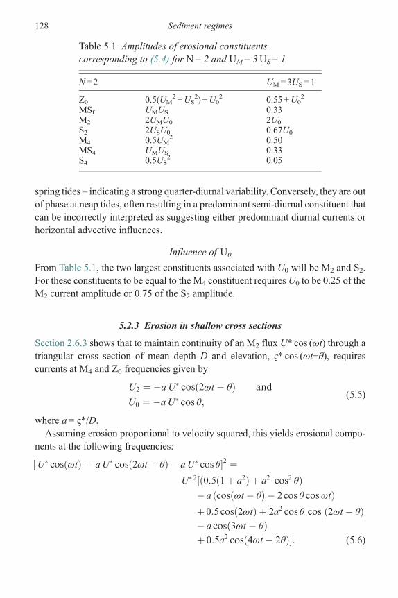
spring tides – indicating a strong quarter-diurnal variability. Conversely, they are outof phase at neap tides, often resulting in a predominant semi-diurnal constituent thatcan be incorrectly interpreted as suggesting either predominant diurnal currents orhorizontal advective influences.

Influence of U0

From Table 5.1, the two largest constituents associated with U0 will be M2 and S2.For these constituents to be equal to the M4 constituent requires U0 to be 0.25 of theM2 current amplitude or 0.75 of the S2 amplitude.

5.2.3 Erosion in shallow cross sections

Section 2.6.3 shows that to maintain continuity of an M2 flux U* cos (ωt) through atriangular cross section of mean depth D and elevation, ς* cos (ωt−θ), requirescurrents at M4 and Z0 frequencies given by

U2 ¼ �aU� cosð2ωt� θÞ and

U0 ¼ �aU� cos θ;(5:5)

where a= ς*/D.Assuming erosion proportional to velocity squared, this yields erosional compo-

nents at the following frequencies:

½U� cosðωtÞ � aU� cosð2ωt� θÞ � aU� cos θ�2 ¼U� 2½ð0:5ð1þ a2Þ þ a2 cos2 θÞ

� a ðcosðωt� θÞ � 2 cos θ cosωtÞþ 0:5 cosð2ωtÞ þ 2a2 cos θ cos ð2ωt� θÞ� a cosð3ωt� θÞþ 0:5a2 cosð4ωt� 2θÞ�: (5:6)

Table 5.1 Amplitudes of erosional constituentscorresponding to (5.4) for N=2 and UM=3US = 1

N = 2 UM=3US = 1

Z0 0.5(UM2 +US

2) +U02 0.55 +U0

2

MSf UMUS 0.33M2 2UMU0 2U0

S2 2USU0 0.67U0

M4 0.5UM2 0.50

MS4 UMUS 0.33S4 0.5US

2 0.05

128 Sediment regimes

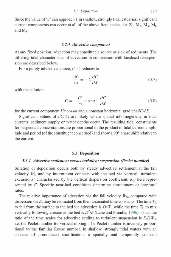
Since the value of ‘a’ can approach 1 in shallow, strongly tidal estuaries, significantcurrent components can occur at all of the above frequencies, i.e. Z0, M2, M4, M6

and M8.

5.2.4 Advective component

At any fixed position, advection may constitute a source or sink of sediments. Thediffering tidal characteristics of advection in comparison with localised resuspen-sion are described below.For a purely advective source, (5.1) reduces to

dC

dt¼ �U

@C

@X(5:7)

with the solution

C ¼ �U�

ωsinωt

@C

@X(5:8)

for the current component U* cosωt and a constant horizontal gradient ∂C/∂X.Significant values of ∂C/∂X are likely where spatial inhomogeneity in tidal

currents, sediment supply or water depths occur. The resulting tidal constituentsfor suspended concentrations are proportional to the product of tidal current ampli-tude and period (of the constituent concerned) and show a 90° phase shift relative tothe current.

5.3 Deposition

5.3.1 Advective settlement versus turbulent suspension (Peclet number)

Siltation or deposition occurs both by steady advective settlement at the fallvelocity WS and by intermittent contacts with the bed via vertical ‘turbulentexcursions’ characterised by the vertical dispersion coefficient, Kz, here repre-sented by E. Specific near-bed conditions determine entrainment or ‘capture’rates.The relative importance of advection via the fall velocity WS, compared with

dispersion via E, may be estimated from their associated time constants. The time TAto fall from the surface to the bed via advection is D/WS while the time TE to mixvertically following erosion at the bed is D2/E (Lane and Prandle, 1996). Thus, theratio of the time scales for advective settling to turbulent suspension is E/DWS,i.e. the Peclet number for vertical mixing. The Peclet number is inversely propor-tional to the familiar Rouse number. In shallow, strongly tidal waters with anabsence of pronounced stratification, a spatially and temporally constant

5.3 Deposition 129

approximation to the vertical eddy viscosity and eddy dispersion coefficients canconveniently be represented by (Prandle, 1982):

Kz ¼ E ¼ fU�D; (5:9)

where f, the bed friction coefficient, is approximately 0.0025 and U* is the tidalcurrent amplitude. The Peclet number is then f U*/WS.Assuming axial and lateral homogeneity allows the terms involving horizontal

advection in (5.1) to be neglected. A ‘single-point’ vertical distribution of sus-pended sediments can then be described by the dispersion equation:

@C

@tþWs

@C

@Z¼ E

@2C

@Z2� sinks þ sources; (5:10)

where the sediment fall velocity Ws replaces the (small) vertical velocity W.

5.3.2 Bottom boundary conditions

Amajor difficulty in numerical simulations of suspended sediments based on (5.10)is the representation of conditions close to the bed, where sharp gradients can existfor both E and Ws (flocculation) and hence in concentration. Appendix 5A showsthat the assumption of settlement at the rate Ws Co is generally twice the valuepertaining with a Gaussian vertical sediment distribution where dispersion counter-acts half of this advective settlement.The use here of an analytical solution avoids the sensitivity, encountered in

numerical schemes, to the precise discretisation of the near-bed region. However,questions still arise as to the extent to which suspended particles rebound or settle oncollision with the bed. Sanford and Halka (1993) provide a comprehensive analysisof alternative bottom boundary conditions.Three conditions are examined in Appendix 5A:

[A] A fully reflective bed. Settlement occurs via advection at the rate 0.5WSCo. Dispersivecollisions with the bed rebound.

[B] A fully absorptive bed. Like condition [A], except that all dispersive collisions settle.[C] Like [A], except that there is additional settlement, by dispersion, of those particles

which have previously been reflected from the surface. This solution is an expedientapproximation, providing solutions intermediate between [A] and [B].

The effect of these three boundary conditions on the rate of deposition is illustratedin Fig. 5.2 (Prandle, 1997a).For E/DWS < 1, Fig. 5.2 and Appendix 5A show that the deposition rate, of

0.5WSC0, is the same for all three conditions.

130 Sediment regimes

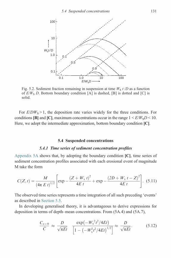
For E/DWS > 1, the deposition rate varies widely for the three conditions. Forconditions [B] and [C], maximum concentrations occur in the range 1 < E/WSD < 10.Here, we adopt the intermediate approximation, bottom boundary condition [C].

5.4 Suspended concentrations

5.4.1 Time series of sediment concentration profiles

Appendix 5A shows that, by adopting the boundary condition [C], time series ofsediment concentration profiles associated with each erosional event of magnitudeM take the form

CðZ; tÞ ¼ M

ð4π E tÞ1=2exp�ðZþWs tÞ2

4E tþ exp�ð2DþWs t� ZÞ2

4E t

" #: (5:11)

The observed time series represents a time integration of all such preceding ‘events’as described in Section 5.5.In developing generalised theory, it is advantageous to derive expressions for

deposition in terms of depth–mean concentrations. From (5A.4) and (5A.7),

Cz¼ 0

�C� Dffiffiffiffiffiffiffiffi

πEtp exp �Ws

2t2=4Et� �

1� �W2s t

2=4Et� �1=2h i � Dffiffiffiffiffiffiffiffi

πEtp : (5:12)

Wst / D

0.1

0.5

0.9

100

10

1.0

0.1

0.1 1.0 10 100E/WsD

Fig. 5.2. Sediment fraction remaining in suspension at time WS t /D as a functionof E/WS D. Bottom boundary condition [A] is dashed, [B] is dotted and [C] issolid.

5.4 Suspended concentrations 131

Thus, a deposition rate expressed asWsCz= 0 transforms to 0:56Ws D=Eð Þ1=2 �C=t1=2� �

when related to depth-averaged concentrations.

5.4.2 Exponential deposition, half-lives in suspension, t50

Approximating deposition of an initial suspended concentration C0 by an exponen-tial loss rate C0e

−αt enables simple analytical expressions to be derived for the timeseries of combined erosion and deposition over successive tidal cycles. Suchan exponential decay rate corresponds to a half-life in suspension t50 = 0.693/α.

For E/WsD < 1.

It is shown in Appendix 5A, (5A.7) and from Fig. 5.2, that the fraction ofsediment remaining in suspension FR approximates

FR ¼ 1� 0:5W2

s t

E

� �1=2

: (5:13)

Equating (5.13) to e− αt for FR = 0.5 requires

α ¼ 0:693W2

s

E:

For E=WsD41

(5:14)

Adopting condition [C], Appendix 5A indicates an expression for thehalf-life t50 = 0.693/α, i.e. the time required for 50% deposition is equivalent to

α ¼ 0:1E

D2: (5:15)

For implementation of (5.14) and (5.15), a continuous transition can be obtained bysimple curve fitting of the results shown in Fig. 5.2. Thus, the parameter α can beclosely approximated by

α ¼ 0:693Ws=D

10x; (5:16)

where x is the root of the equation:

x2 � 0:79xþ jð0:79� jÞ � 0:144 ¼ 0 (5:17)

with j = log10E/WsD.

Assuming the following relationship between fall velocity WS and particlediameter d

Ws ðms�1Þ ¼ 10�6 d 2 ðμmÞ: (5:18)

132 Sediment regimes

Figure 5.3 illustrates corresponding half-lives in suspension for WS = 0.005 and0.0005m s−1, i.e. d= 71 and 22 μ, as functions of tidal current amplitude and depth.Thus, for sand, half-lives range from a minute in sluggish shallow water to 2 h indeep strongly tidal waters. For fine silt, these values range from hours in shallowwater to 2 days in deep water.More generally, using dynamical solutions for a ‘synchronous’ estuary, Fig. 7.6

indicates values of α ranging for sand from l0−3 to 10−2 s−1 corresponding to valuesfor t50 of 10–1m. The equivalent values for fine silt and clay are α from 10−6 to10−4 s−1 for t50 of 200–2 h.An important result is that for the finer sediment, the half-life in suspension is

almost always of order (6 h) or greater. This implies that where estuarine sedimentregimes are maintained by the influx of fine marine sediments, these will remain innear-continuous suspension and so their distributions will share features of acontinuously suspended conservative tracer such as salt.To further illustrate the characteristics and significance of this parameter E/WSD, we

use (2.19) to relate tidal current amplitudes U* to elevation amplitude ζ*. Figure 5.4(Prandle, 2004) then shows, for D=8m, the relationship between WS and E/WSDfor ζ*=1, 2 and 3m, i.e. almost the complete range of tidal conditions encountered.

2 h

1 h

10 h

20 h

50 h

1 h

15 m

5 m

1 m

Fall velocity ws = 0.005 m s–1 Fall velocity ws = 0.0005 m s–1

Tidal

cur

rent

am

plitu

de (

m s

–1)

Tidal

cur

rent

am

plitu

de (

m s

–1)

2.0

1.0

00 10 20 30 40

Depth (m)

2.0

1.0

00 10 20 30 40

Depth (m)

Fig. 5.3. Half-lives, t50, of SPM in suspension as f (D,U*). (Left) Sand,WS = 0.005m s−1, (right) silt, WS = 0.0005m s−1. t50 = 0.693/α, α from (5.16).

5.4 Suspended concentrations 133

This illustrates how the demarcation line of E/WSD ≈ 1 coincides with fall velo-cities of order of (1mm s−1) or, from (5.18), d = 32 μ. It also shows how the valueof E/WS D lies in the range from 0.1 to 10 for sediment diameters in the range20–200 μ. Hence, the approximation, (5.16), for α, based on Fig. 5.2, should bewidely applicable.

5.4.3 Vertical profile of suspended sediments

It is shown in Appendix 5A that for E/DWS < 0.3, less than 1% of particles reach thesea surface, whereas for E/DWS > 10, suspended sediments are well mixed verti-cally. Thus, throughout the range of conditions considered, clay is always likelyto be well mixed vertically, whereas sand will be confined to near-bed regions fortidal velocity amplitudes U*≤ 0.5m s−1. Likewise, pronounced vertical structurethroughout the water column is likely for silt when U* ≤ 0.5m s−1.A continuous functional description of the vertical profiles of suspended sedi-

ment concentrations was calculated by Prandle (2004) by numerical fitting of aprofile e−β z (where z is the fractional height above the bed) to simulations based on(5.12). The following expression for β was derived:

β ¼ 0:91 log10 6:3E

DWs

� �� ��1:7

�1: (5:19)

Figure 5.5(a) (Prandle, 2004) shows values of β over the range E/DWS from 0 to 2.Figure 5.5(b) shows corresponding values of sediment profiles e−βz (1−e−β)/β,

0.05

0.005

0.00050 1 2 3 4 5

E /WsD

ζ = 2 mζ = 1 m

ζ = 3 m

Ws

∧ ∧

∧

Fig. 5.4. Fall velocityWS (m s−1) as a function of E/WsD tidal elevation amplitudesζ* = 1, 2 and 3m; results are for depth D = 8m.

134 Sediment regimes

illustrating how effective complete vertical mixing is achieved for E/DWS > 2, and‘bed load’ only occurs for E/DWS < 0.1. (Concentration profiles are normalisedrelative to the depth-averaged value.)

5.5 SPM time series for continuous tidal cycles

The concentration C(t) associated with erosion varying sinusoidally at a rate ofcosωt subject to an exponential decay rate –αC involves integration over allpreceding time t 0 from –∞ to t, that is

CðtÞ ¼ðt

�1cos ωt0e�αðt�t0Þdt0 ¼ α cosωtþ ω sinωt

α2 þ ω2: (5:20)

Hence, from (5.2), the concentration, Cω, for any erosional constituent, ω, isgiven by

Cω ¼ γ f ρ ½UN�ωDðω2 þ α2Þ1=2

; (5:21)

where [UN]ω is the erosional amplitude at frequency ω as shown in Table 5.1for N= 2.Thus, erosion generated at each of the tidal constituents in the expansion of

source terms is subsequently modulated by an exponential decay rate that involvesan amplitude reduction by the factor (α2 +ω 2)−1/2 and a phase-lag of arctan (ω/α).

0.1

0.9

1

1.1

210

0.5

1

00 1 2

zβ

5(a) (b)

4

3

2

1

00 1 2

K z /WsDK z /WsD

Fig. 5.5. Concentration profiles and values of β described by sediment profile e−βz,(5.19). (a) Values of β as a function of Kz/WSD. (b) Corresponding profiles;contours are fractions of depth-mean concentrations, surface is z = 1.

5.5 SPM time series for continuous tidal cycles 135

The response function represented by (5.20) is shown inFig. 5.6 (Prandle, 1997b) for arange of values ofα andω from10−7 to 1 s−1. For α≫ω, the amplitude of the responseis proportional only to 1/α with zero phase lag. Conversely, for ω≫ α, the amplitudeof the response is proportional only to the period concerned with a 90° phase lag.Thus, for equal amounts of eroded sand (α� 10−3 s−1) and silt/clay (α� 10−6 s−1),

away from the immediate vicinity of the bed, the amplitude ratios of the suspendedsediment tidal signal for sand are always much smaller than for silt/clay.Within this silt/clay fraction, the ratio of the SPM tidal constituent amplitudes is

determined by the product of (i) the ratios shown in Table 5.1 and (ii) the duration ofthe tidal periods concerned. These amplitudes are largely independent of the specificvalue of α (within the range concerned). Likewise, for this silt/clay fraction, thephases are lagged by 90° in the quater-diurnal to diurnal tidal band. Thus, factoringthe amplitudes in Table 5.1 by tidal period, we expect the MSf, 15 days cycle topredominate followed by M4 and MS4. Phase values of up to 90° for MSf indicateassociated maximum suspended sediment concentrations occurring up to 3.5 daysafter maximum currents. Conversely, phase values approaching 0° for M2 and S2indicate associated maximum suspensions in phase with maximum currents.

10–1 101

102

103

5°45°

85°

104

105

106

11

10–2

10–3

10–4

10–5

10–6

ω (s–1)

α (s–1)

10–6 10–5 10–3 10–2 10–1 110s1D15D1Y D/2 D/4

SAND

SILT&CLAY

Fig. 5.6. Concentration amplitudes for unit erosion at cyclic frequencies ω fordeposition rate e−αt. Solid contours indicate relative amplitudes and dashed linesphase lag between SPM and erosion (5.20).

136 Sediment regimes

For ω≫ α, the Z0 constituent is factored by ω/α relative to the tidal frequency.Thus, by using the Z0/MSf ratio derived from observations alongside the expansionsshown in Table 5.1 and (5.20), a direct estimate of α can be obtained.

5.6 Observed and modelled SPM time series

5.6.1 Observational technologies

Observations are crucial to developing and assessing SPM models. In situ con-centrations are routinely monitored acoustically, optically and mechanically.Acoustic backscatter (ABS) probes provide vertical profiles of concentration,multi-frequency probes provide information on grain size – usually at a singlepoint. Pumped samples, bottles and traps are used in mechanical devices. Recentdevelopments of in situ laser particle sizers provide valuable information onparticle spectra non-invasively (mechanical samplers can corrupt these spectra).Available observations suffer from fundamental shortcomings, namely (i) calibra-

tion from sensor units to concentration involving complex sensitivity to particle sizespectra in optical and acoustic instruments and to atmospheric corrections and sunangle effects in remote sensing; (ii) unresolved particle-size spectra and (iii) limitedspatial and temporal coverage relative to the inhomogeneity of sediment distributions.The spatial resolution of in situ concentration measurements is generally limited

to single points (or limited profiles) in optical backscatter (OBS) and ABS sensorsand to surface values from satellite or aircraft sensors. Techniques to circumventthese shortcomings are described by Gerritsen et al. (2000) where the spatialpatterns of surface imagery are used to validate models.Each instrument has its own calibration peculiarities. Moreover, all of these

calibrations vary as the mean particle size changes. Optical devices rely on occlu-sion of light – transmittance or reflectance (OBS). Since this is dependent onthe surface area of the particle, recordings are more sensitive to finer scale particles.Hence, observed concentrations need to be calibrated by reference to some represen-tative particle radius. The plate-like character of flocs complicates such calibrations.Conversely, ABS (in the range of frequencies used in ABS instruments) increases

with particle volume, and hence, these instruments are more sensitive to coarseparticles. The optical instruments also experience fouling, and all of the instrumentscan be swamped above certain concentrations.Satellite images of (surface) SPM concentrations can be used in conjunction with

model simulations to infer the magnitude of discrete sediment sources. Aircraftsurveillance using multi-wavelength imagery can differentiate between the reflec-tance from SPM associated with chlorophyll and that from various sediment frac-tions. However, the need for atmospheric corrections introduces some reliance on insitu calibrations.

5.6 Observed and modelled SPM time series 137

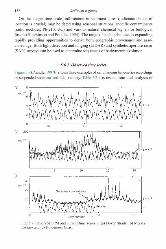
On the longer time scale, information in sediment cores (judicious choice oflocation is crucial) may be dated using seasonal striations, specific contaminants(radio nuclides, Pb-210, etc.) and various natural chemical signals or biologicalfossils (Hutchinson and Prandle, 1994). The range of such techniques is expandingrapidly providing opportunities to derive both geographic provenance and asso-ciated age. Both light detection and ranging (LIDAR) and synthetic aperture radar(SAR) surveys can be used to determine sequences of bathymetric evolution.

5.6.2 Observed time series

Figure 5.7 (Prandle, 1997b) shows three examples of simultaneous time-series recordingsof suspended sediment and tidal velocity. Table 5.2 lists results from tidal analyses of

200

0

30

20

10

0

Day number

Sediment concentration

Velocity

0 5 10 15

0

1 m s –1

0

1 m s –1

5 10 15 20

8

6

4

2

010 15 20

0

2 m s–1

(a)

mg I–1

mg I–1

mg I–1

(b)

(c)

Fig. 5.7. Observed SPM and current time series in (a) Dover Straits, (b) MerseyEstuary and (c) Holderness Coast.

138 Sediment regimes

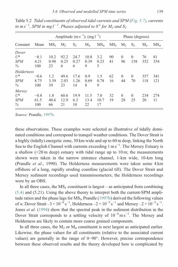
these observations. These examples were selected as illustrative of tidally domi-nated conditions and correspond to tranquil weather conditions. The Dover Strait isa highly (tidally) energetic zone, 30 km wide and up to 60m deep, linking the NorthSea to the English Channel with currents exceeding 1m s−1. The Mersey Estuary isa shallow (<20m deep) estuary with tidal range up to 10m; the measurementsshown were taken in the narrow entrance channel, 1-km wide, 10-km long(Prandle et al., 1990). The Holderness measurements were taken some 4 kmoffshore of a long, rapidly eroding coastline (glacial till). The Dover Strait andMersey sediment recordings used transmissometers; the Holderness recordingswere by an OBS.In all three cases, the MSf constituent is largest – as anticipated from combining

(5.4) and (5.21). Using the above theory to interpret both the current-SPM ampli-tude ratios and the phase lags for MSf, Prandle (1997b) derived the following valuesof α: Dover Strait –3 × 10−6 s−1, Holderness –2 × 10−5 s−1 and Mersey –2 × 10−5 s−1.Jones et al. (1994) show that the spectral peak in the sediment distribution in theDover Strait corresponds to a settling velocity of 10−4m s−1. The Mersey andHolderness are likely to contain more coarse grained components.In all three cases, the M2 or M4 constituent is next largest as anticipated earlier.

Likewise, the phase values for all constituents (relative to the associated currentvalues) are generally in the range of 0−90°. However, precise correspondencebetween these observed results and the theory developed here is complicated by

Table 5.2 Tidal constituents of observed tidal currents and SPM (Fig. 5.7), currentsin m s−1, SPM in mg l −1. Phases adjusted to 0 o for M2 and S2

Amplitude (m s−1); (mg l−1) Phase (degrees)

Constant Mean MSf M2 S2 M4 MS4 MSf M2 S2 M4 MS4

DoverU* −8.1 10.2 92.2 24.7 10.8 3.2 90 0 0 76 81SPM 4.21 0.98 0.25 0.27 0.39 0.23 41 96 158 352 354% 100 23 6 6 9 5

HoldernessU* −0.6 1.2 49.6 17.6 0.9 1.5 62 0 0 357 341SPM 8.75 3.39 2.03 1.26 0.69 0.78 16 44 70 118 121% 100 39 23 14 8 9

MerseyU* −0.8 1.8 60.6 19.9 11.5 7.0 32 0 0 234 274SPM 61.5 40.6 12.9 6.3 13.4 10.7 19 28 25 20 11% 100 66 21 10 22 17

Source: Prandle, 1997b.

5.6 Observed and modelled SPM time series 139

such factors as the spectral width of settling velocities of the particles involved,finite supply, advection and vertical variations in concentration.The mean concentration in the Mersey is an order of magnitude higher than in the

Dover Strait. Concentrations at Holderness lie between these two. Thus, there is asuggestion of limited supply in the Dover Strait; moreover, the phase relationshipfor the M2 constituent is indicative of a significant advective component.

5.6.3 Modelled time series

Figure 5.8 (Prandle, 2004) shows characteristic model-generated spring–neap cyclesof SPMassociatedwith localised resuspension in a tidally dominated estuary (Prandle,1997a) for E=Kz = 0.1 and 10 WSD. For E=0.1 WSD, particles scarcely reach thesurface and with a short half-life in suspension, the quarter-diurnal constituentpredominates. Conversely for E=10 WSD, particles are evenly distributed through

= 0

= 0

= 0

= 0

= 0

E/DWs = 0.1

E/DWs = 10

Con

cent

ratio

nC

once

ntra

tion

C10

C9

C8

C7

C6

C5

C4

C3

C2

C1

Days

0 1 2 3 4 5 6 7 8 9 10 11 12 13 14 15

Fine particle

Coarse particle

C10

C9

C8

C7

C6

C5

C4

C3

C2

C1

Fig. 5.8. Model simulations of SPM over a spring–neap tidal cycle. C1, C2,… , C10concentrations at fractional heights z1/2 = 0.05–0.95. (Top) Kz /DWS = 0.1; (bottom)Kz /DWS = 10.

140 Sediment regimes

the water column and the extended half-life in suspension amplifies the MSfconstituent relative to M4.

Fine resolution 3D estuarine models of tidal propagation can provide reliable andaccurate simulations of water levels and flows, often limited only by inadequacies inthe accuracy and resolution of the bathymetry. Likewise, recent developments incoupling these tidal dynamics with turbulence-closure modules provide good,detailed descriptions of current structure. However, fundamental uncertainties inmodelling SPM fluxes arise from (i) insufficient information on surficial sedimentdistributions; (ii) the inherent complexities of erosion and deposition processes –especially regarding the influence of flocculation and (iii) the paucity of observa-tional data for calibration/evaluation. Algorithms relating bed stresses with rates oferosion are plentiful but cannot easily embrace the full range and mixture of bedmaterials or the chemical and biological influences. Likewise, in conditions of high(near-bed) concentrations, sediment particles interact (flocculation and hinderedsettlement) modifying both the dynamics and the wider sediment regime.The biggest difficulty in long-term simulations of SPM in estuaries is the

specification of the available sources of sediments – internal, coastal, riverine andorganic. Lack of information on particle size distributions of suspended sediments isa major deficiency along with ignorance of the nature and distribution for surficialsediments. The use of aircraft surveillance to provide SPM distributions (sea sur-face) may, via assimilation techniques, help to address this issue. While large area,long-term model simulations can link these sources, specific sequences of eventsneed to be reproduced – resulting in practice in accumulation of errors.The ultimate goal is to understand the evolving morphological equilibrium

between bathymetry and the prevailing tidal currents, waves and mean sea level.Simulating net long-term bathymetric evolution is especially difficult, since itinvolves the net temporal integration of the spatial divergence of all simulations.The requirement for models to reproduce near-zero net accretion and erosionprovides a demanding criterion. It is generally concluded that extrapolation usingprimitive equation (bottom-up) models is severely limited. Arguably, such modelsshould only be used to indicate pathways and likelihoods of erosion/accretion forperiods of a few years ahead. Further extrapolation often makes use of geomorpho-logical (top-down) models which derive stability rules based on geological evidenceof coastal movements. Bottom-up models can be used to test the validity of thesetop-down rules in any particular estuary.The scope of monitoring, modelling and theoretical developments described

highlights the need for collaboration interdisciplinary and internationally. Thevalue of basic process studies in near-full scale flumes alongside extended estuarialobservational campaigns is evident. Such data need to be quality assured and storedsystematically for accessible dissemination. Permanent comprehensive observational

5.6 Observed and modelled SPM time series 141

networks exploiting synergistic aspects of a range of instruments/platforms inte-grally linked to modelling requirements/capabilities are especially valuable. Theultimate derivation of robust, portable SPM models depends on the availability ofa range of such data sets from a wide range of estuaries, i.e. parallel programmesacross estuaries with varying latitudes, scales, geological types and environmentalexposures.

5.7 Summary of results and guidelines for application

Focusing on strongly tidal estuaries, by integrating erosion, suspension and deposition,analytical solutions are derived describing suspended sediment time series andtheirvertical structure. The related scaling parameters indicate the sensitivities to sedimenttype, tidal current speed and water depth, providing insight into and interpretation ofsediment regimes obtained from observations or numerical simulations.

The leading question addressed is:

How are the spectra of suspended sediments determined by estuarine dynamics?

The major interest with sediment regimes in estuaries generally concernsbathymetric evolution. Additional ecological interests include (i) the transport ofcontaminants by adsorption onto fine sediments and (ii) light occlusion from highconcentrations of suspended sediments. Geologists examine morphological evolutionover millions of years and geomorphologists over millennia. Conversely, coastalengineers are concerned with relatively immediate impacts following extreme‘events’ or ‘interventions’ and decadal adjustments to changes in msl and otherlong-term trends. Chapter 7 introduces a link between present-day morphologicalequilibria and historical changes in msl since the last ice age.The earliest engineering studies of sediment transport were concerned with

maintaining bathymetric equilibrium in the unidirectional flow regimes of irrigationand navigation canals. By contrast, one of the notable features in strongly tidaloscillatory regimes is the persistence over decades and re-emergence (after extremeevents or ‘intervention’) of bathymetric features such as spits, pits and systematicinter-tidal forms.Compared with tidal elevations, currents and salinity, suspended sediments

exhibit extreme variability. This embraces (i) size, ranging from fine to coarsewith particle diameters ranging from clay < 4 μ, silt < 60 μ, sand < 1000 μ togravels; (ii) temporal, spanning flood to ebb, neap to spring tides, from tranquil tostorm conditions with related extreme values of water levels, velocities, waves andriver flows; (iii) spatial, extending vertically, axially and transversally. Even withoutthe technical difficulties of measuring concentrations of SPM, conditions justmetres apart can show dramatic differences, reflecting the sensitivity to water

142 Sediment regimes

depth, current speed, waves, turbulence intensity and surficial sediment distribu-tions with their attendant bed features.Recognising such intrinsic variability, the present approach is limited in scope,

concentrating on first-order effects in strongly tidal regimes. This focus represents atractable component of sediment dynamics, involving variability in concentrationson logarithmic scales and exploiting robustly determinable tidal characteristics.For a wider perspective, many additional features need to be considered, includingthe chemistry of fine particles (Partheniades, 1965), near-bed interactions betweenflow dynamics and sediments for coarse particles (Soulsby, 1997), wave–currentinteractions (Grant and Madsen, 1979) and the impacts of bed features (Van Rijn,1993). Useful summaries are described by Davies and Thorne (2008) and Van Rijn(2007(a),(b) and (c)).Postma (1967) emphasised the significance, in estuaries, of the separation

between erosion at one location and the subsequent ‘delayed’ settlement at positionsas far apart as the tidal excursion. Here, we aim to determine representative valuesof these delays, encapsulated by the ‘half-life’ of sediment in suspension, t50.Rejecting the traditional demarcation into periods of erosion and deposition sepa-rated by thresholds of velocity or bed stress, ‘single-point’ analytical solutions forthe simultaneous processes of erosion, suspension and deposition are derived.Similarly, the plethora of complicated formulae for erosion and settlement aresimplified, with erosion related to some power of tidal velocity and deposition tothe depth–mean concentration multiplied by an exponent based on the half-life insuspension.By assuming that eddy diffusivity Kz and eddy viscosity E can be approximated by

Kz =E= fU*D, (3.23), these solutions indicate how the essential scaling of sedimentmotion is synthesised in the dimensionless parameter E/WSD as shown in Figs (5.4),(5.5) and (5.8), (where f is the bed friction coefficient, D is water depth, U* tidalcurrent amplitude andWS sediment fall velocity). Turbulent diffusion, parameterisedby the coefficient E, promotes the suspension of particles by random vertical oscilla-tions, whereas the fall velocity WS represents steady advective settlement. The timetaken for a particle to mix vertically by dispersion is D2/E whereas settlement byvertical advection occurs withinD/WS. Thus, the ratio of E :WSD reflects the relativetimes of deposition by advective settlement to that by diffusive vertical excursions.

5.7.1 Sediment suspension

For E < 0.1 WS D, particles are confined to the near-bed region, whereas for E >10WS D, particles are evenly distributed throughout the water column (Fig. 5.8).Approximating settling velocities by sand, WS = 10

−2m s−l; silt, WS = 10−4m s−1;

and clay, WS = 10−6m s−1, it is shown that generally, sand is concentrated near the

5.7 Summary of results and guidelines for application 143

bed, clay is well mixed vertically and silt shows significant vertical structure.Assuming a sediment concentration profile e−βz, an expression, (5.19), for β interms of E/WS D is derived. Corresponding vertical profiles are shown in Fig. 5.5.

5.7.2 Deposition

The rate of deposition is expressed by the function Ce−αt, where α= 0.693/t50represents the exponential settling rate.For E≪WSD, deposition is by advective settlement at a rate (1/2)WSC0

and α� 0.7 WS2/E, (5.14). The fractional rate of deposition is determined by (l/2)

[(WS2t)/E]1/2, i.e. 10% after 0.04E/WS

2, 50% after E/WS2 and 90% after 3.2E/WS

2

(Appendix 5A).For E≫WSD, deposition is independent of WS but dependent on both

the magnitude of the vertical dispersion coefficient and the precise near-bed condi-tions. Using an expedient bottom boundary condition, the value α� 0.1E/D2 isderived (5.15).As E→WS D, the mean time in suspension approaches a maximum and hence

both mean concentration and net transport will increase. Section 7.3.1 shows thatthis condition occurs for WS� 1mm s−1, i.e. particle diameter d� 30 μ.Equation (5.17) provides a continuous expression for α across the full range of

E/WSD.

5.7.3 Tidal spectra of SPM

By integrating the above analytical solutions for SPM concentrations over succes-sive tidal cycles, the spectrum of suspended sediments is calculated, (5.20). Thecharacteristics of this spectrum are determined by the ratio of the exponentialsettlement rate, α, to the frequency of the erosional tidal currents, ω (Fig. 5.6). Forα > 10ω, the suspended sediment tidal amplitude is proportional to 1/α with zerophase lag of SPM relative to current. Whereas, for ω > l0α, the amplitude isproportional to tidal period (1/ω) with a 90° phase lag.From (5.18) and Fig. 5.3, for sand 10−2 > α > 10−3 s−1 and 1m < t50 < 10m, hence

the former condition applies and the amplitude response at all tidal frequencies ismuch reduced.For silt and clay, 10−4 > α > 10−6 s−1 and 2 h < t50 < 200 h. Since the major tidal

constituents lie in the range ω ≥ 10−4 s−1, the cyclical amplitude response is rela-tively independent of α but proportional to tidal period, resulting in an enhancementof longer period constituents. Wherever there is a plentiful supply of erodiblesediment of a wide size distribution, the resulting suspended sediment time seriesaway from the immediate near-bed area is likely to be dominated by silt–clay.

144 Sediment regimes

In the absence of significant residual currents, the erosional time series for anM2−S2-dominated tidal regime will show pronounced components at M4, MS4, MSfand Z0 frequencies, (5.4) and Table 5.1. These latter components are generated bynon-linear combinations of M2 and S2 currents and not by any (usually small) tidalcurrent amplitudes at these emergent frequencies. The similarity in amplitudes ofthe M4 and MS4 constituents may reduce the quarter-diurnal signal at neap tides(when their phases are opposed) and thereby suggest an enhanced semi-diurnalsediment signal that might be wrongly interpreted as indicating horizontal advectionor a large diurnal current component. When ‘residual currents’ increase to a level oforder 10% of the M2 amplitude (as in strongly tidal shallow waters), the suspendedsediment time series will include M2 and S2 constituents of comparable magnitudeto those described for M4, MS4 and MSf. Over a spring–neap tidal cycle, for E > 10WS D, the peak in suspended sediment concentration will generally occur 2–3 daysafter the occurrence of maximum tidal currents.In summary, the theory (Table 5.1 and Fig. 5.6) explains how tidal spectra

shown in SPM observations (Table 5.2 and Fig. 5.7) are modulated relative to thatof the generating current spectra. The associated amplitude ratios and phase lagsshown in such observations can be used to infer both the nature of the predominantsediment type and the roles of localised resuspension versus advection.

Appendix 5A

5A.1 Analytical expression for sediment suspension

An expression is derived for the time sequence of sediment suspension, linkingerosion through to deposition as a function of three variables, namely settlingvelocity WS, vertical dispersion coefficient E and water depth D.

5A.2 Dispersion equation

It is assumed that the distribution of suspended sediments can be described by thedispersion equation; moreover, in the present application, consideration is limited tomotion in one horizontal direction, X. Thence, the version of (5.1) representing therate of change in concentration C is

dC

dt¼ @C

@tþU

@C

@XþW

@C

@Z¼ @

@ZE@C

@Z� sinksþ sources; (5A:1)

where t is time,U horizontal velocity,W vertical velocity, Z the vertical axis measuredupwards from the bed and E a vertical dispersion coefficient. Horizontal dispersion isnot considered, and E is assumed to remain constant both temporally and vertically.Equation (5A.1) can be converted to convenient variables as follows:

Appendix 5A 145

z ¼ Z

D; w ¼ W

D; e ¼ E

D2;

where D is the water depth, z= 0 is the bed and z= 1 the surface. By assuminghorizontal homogeneity, i.e. ∂C/∂X= 0, (5A.1) may be rewritten:

@C

@tþ w

@C

@z¼ e

@2C

@z2� sinksþ sources: (5A:2)

Equation (5A.2) can then be used to describe the transport of particulate material bysetting the vertical velocity W in (5A.1) equal to the settling velocity −Ws.

5A.3 Analytical solutions

Fischer et al. (1979) show that the general solution for dispersion of a tracer of massM (confined to 1D Z) released at Z= 0, t = 0 in a fluid moving at a velocity W is

CðZ; tÞ ¼ Mffiffiffiffiffiffiffiffiffiffi4πEt

p exp�ðZ�WtÞ24Et

: (5A:3)

It is convenient to introduce variables t0 =ws t and z0 = z + ws t. Rewriting (5A.3) inthese variables, the concentration at z0 is

Cðz0; tÞ ¼ M

Dffiffiffiffiffiffiffiffiffiffiffiffiffi4π e

wst0

q exp�z02

4 ewst0

!: (5A:4)

Since (Fischer et al., 1979),

ðz

0

e�z2dz ¼ffiffiffiπ

p2

ERFðzÞ; (5A:5)

the net amount of sediment in suspension between z0 = 0 and z0 is

TS ¼ D

ðz0

0

CðzÞ dz ¼ M0 ERFz0ffiffiffiffiffiffiffiffiffiffiffi4 ewst0

q

0B@

1CA; (5A:6)

where M 0= M/2 corresponds to the amount of eroded suspended above the bedat t = 0.The value of the error function in (5A.6) must always be less than 1. Then, since

for 0 < x < 1, ERF(x)� x, the net amount deposited at z= 0 after time t0 is given bysubstituting z0 = t0 in (5A.6), i.e.

146 Sediment regimes

TS � M0

2

t0

ð ewst0Þ1=2

: (5A:7)

From (5A.7), after t0 = 0.04 e/ws, TS= 0.1M0; after t0 = e/ws, TS= 0.5M0 while aftert0 = 3.2 e/ws, TS= 0.9M0. These deposits can be separated into an advective compo-nent due to Ws in (5A.3) and a dispersive component associated with E.By successively differentiating the corresponding top and bottom terms in (5A.7)w.r.t. t, it follows that the advective deposition is a factor of 2 greater and of oppositesign to the dispersive ‘erosion’. From differentiation of (5A.6) w.r.t. z, the rate ofadvective deposition isWS C(z′= 0), i.e. the anticipated net deposition for an absorp-tive bed that retains all particles making contact. The 50% return rate, implicit in(5A.3), infers a continuing dynamic relationship at the bed that persists up to some4e/ws after erosion. Wiberg and Smith (1985) used a ‘rebound coefficient’ ofaround 0.5 to account for partially elastic collisions between moving grains andthe bed.

5A.4 Boundary condition at the surface z= 1

At the surface, a simple reflective boundary condition is introduced involving aghost source (of equal magnitude to the original source) located at z= 2+ wst, i.e.equidistant from the original source at z=−ws t. The ‘first’ (l% of M 0) particlespassing the surface corresponds to

1

M0

ðDð1þwstÞ

0

CðZÞ dZ ¼ 0:99 ¼ ERF

1þ t0ffiffiffiffiffiffiffiffiffiffiffiffi4e

ws

t0r

0B@

1CA: (5A:8)

Equation (5A.8) requires the argument of the error function to equal 1.83, hence realsolutions for t0 require e/ws > 0.3. Thus, for smaller values of e/ws, less than 1% ofparticles reach the surface.

5A.5 Boundary condition at the bed z= 2, 4, 6, etc.

Sediments ‘reflected’ from the surface arrive back at the bed where they may bedeposited or resuspended so long as, by analogy with (5A.8), (2 + t 0) / (4et 0/ws)

1/2 <1.83, i.e. e/ws > 0.6.The ratio, R, of suspended sediments reflected from the surface towards the

bed (i.e. between z0 = 1 + wst and z0 = 2 + wst) to those yet to reach the surface(i.e. between z0 =wst and z0 = 1+ wst) is

Appendix 5A 147

R ¼ Rs

RB

¼ERF

2þ wstffiffiffiffiffiffiffi4et

p� �

� ERF1þ wstffiffiffiffiffiffiffi

4etp

� �

ERF1þ wstffiffiffiffiffiffiffi

4etp

� �� ERF

wstffiffiffiffiffiffiffi4et

p� � : (5A:9)

This ratio shows that for e/ws < 0.1 almost no particles reach the surface.Conversely, for e/ws > 10, there will be little vertical variation in the suspendedsediment concentrations.Three approximations are considered for the bottom boundary condition as

described below.

[A] Fully reflective bedSources of equal magnitude at

INITIALSOURCE

REFLECTIONFROM BED

REFLECTIONFROM SURFACE

z ¼ �wst (1) initial sourceð2þ wstÞ (2) reflection of (1)

�ð2þ wstÞ (3) reflection of (2)

||

�ð2ðn� 1Þ þ wstÞ (2n− 1) reflection of(2n − 2)

ð2nþ wstÞ (2n) reflection of (2n− 1)

Numerically, this series continues until the contribution from the last two terms isnegligible. The condition implies that deposition only occurs at z0 = 0, hence thesolutions to (5A.6) shown by the dashed line in Fig. 5.2 indicate the rate of deposition.

[B] Fully absorptive bedThis requires zero effective concentration at the bed for those sediments arriving afterreflection from the surface, i.e. sources of equal magnitude but opposite sign. Thisresults in a series of sources/sinks as in boundary condition [A], combinations 3, 4; 7, 8,etc. representing sinks.

[C] Termination of the series after two termsSources at

INITIALSOURCE

REFLECTIONFROM BED

REFLECTION FROMSURFACE

z ¼ �wst (1) initial sourceð2þ wstÞ (2) reflection of (1)

Figure 5.2 illustrates the fraction of sediments remaining in suspension at time,wst, after erosion for these three boundary conditions. The three lines that correspondto the bottom boundary conditions [A] is dashed, [B] is dotted and [C] is solid.For values of e/ws < 1.0, the results show little difference since it was shown

earlier that little sediment passes beyond z= 2 for this condition. However, for

148 Sediment regimes

e/ws > 10, the results differ widely and, for the latter two boundary conditions,suspension times decrease with increasing values of e/ws. This implies a greater‘capture rate’ as a result of increased collisions with the bed.As a convenient expedient, we subsequently adopt the third boundary condition

as being someway intermediate between the other two extremes. However, it isrecognised that this expedient reduces the validity of results presented for therange e/ws≫ 1. In practice, the appropriate boundary condition will be a functionof the benthic boundary layer dynamics and of the sediment characteristics andconcentration.Thus, subsequently, we assume sediment concentrations given by

Cðz; tÞ ¼ M

Dð4πetÞ1=2exp � ðzþ wstÞ2

4etþ exp � ð2þ wst� zÞ2

4et

" #: (5A:10)

References

Davies, A.G. and Thorne, P.D., 2008. Advances in the study of moving sediments andevolving seabeds. Surveys in Geophysics, doi:10.1007/S10712-008-9039-X, 36pp.

Fischer, H.B., List, E.J., Koh, R.C.Y., Imberger, J., and Brocks, N.K., 1979. Mixing inInland and Coastal Waters. Academic Press, New York.

Gerritsen, H., Vos, R.J., van der Kaaij, T., Lane, A., and Boon, J.G., 2000. Suspendedsediment modelling in a shelf sea (North Sea). Coastal Engineering, 41, 317–352.

Grant, W.D. and Madsen, O.S., 1979. Combined wave and current interaction with a roughbottom. Journal of Geophysical Research, 84 (C4), 1797–1808.

Hutchinson, S.M. and Prandle, D., 1994. Siltation in the salt marsh of the Dee estuaryderived from 137Cs analyses of short cores. Estuarine, Coastal and Shelf Science,38 (5), 471–478.

Jones, S.E., Jago, C.F., Prandle, D., and Flatt, D., 1994. Suspended sediment dynamics, theirmeasurement and modelling in the Dover Strait. In: (Beven, K.J., Chatwin, P.C.,and Millbank, J.H. (eds), Mixing and Transport in the Environment, John Wiley andSons, New York, pp. 183–202.

Krone, R.B., 1962. Flume Studies on the Transport of Sediments in Estuarine ShoalingProcesses. Hydraulic Engineering Laboratories, University of Berkeley, CA.

Lane, A. and Prandle, D., 1996. Inter-annual variability in the temperature of the North Sea.Continental Shelf Research, 16 (11), 1489–1507.

Lane, A. and Prandle, D., 2006. Random-walk particle modelling for estimating bathymetricevolution of an estuary. Estuarine, Coastal and Shelf Science, 68 (1–2), 175–187.

Lavelle, J.W., Mojfeld, H.O., and Baker, E.T., 1984. An in-situ erosion rate for afine-grained marine sediment. Journal of Geophysical Research, 89 (4), 6543–6552.

Partheniades, E., 1965. Erosion and deposition of cohesive soils. Journal of HydraulicsDivision ASCE, 91, 469–481.

Postma, H., 1967. Sediment transport and sedimentation in the estuarine environment. In:Lauff, G.H. (ed.), Estuaries. American Association for the Advancement of Science,Washington, DC, pp. 158–180.

Prandle, D., 1982. The vertical structure of tidal currents and other oscillatory flows.Continental Shelf Research, 1 (2), 191–207.

References 149

Prandle, D., 1997a. The dynamics of suspended sediments in tidal waters. Journal ofCoastal Research, 40 (Special Issue No 25), 75–86.

Prandle, D., 1997b. Tidal characteristics of suspended sediment concentration. Journal ofHydraulic Engineering, ASCE, 123 (4), 341–350.

Prandle, D., 2004. Sediment trapping, turbidity maxima and bathymetric stability in tidalestuaries. Journal of Geophysical Research, 109 (C8).

Prandle, D., Murray, A. and Johnson, R., 1990. Analysis of flux measurements inthe Mersey River. In: Cheng, R.T. (ed.), Residual currents and Long TermTransport. Coastal and Estuarine Studies, Vol. 38. Springer-Verlag, New York,pp. 413–430.

Romano, C., Widdows, J., Brimley, M.D., and Staff, F.J., 2003. Impact of Enteromorpha onnear-bed currents and sediment dynamics: flume studies. Marine Ecology ProgressSeries, 256, 63–74.

Sanford, L.P. and Halka, J.P., 1993. Assessing the paradigm of mutually exclusive erosionand deposition of mud, with examples from upper Chesapeake Bay. MarineGeotechnics, 114 (1–2), 37–57.

Soulsby, R.L., 1997. Dynamics of Marine Sands: a Manual for Practical Applications.Telford, London.

Van Rijn, L.C., 1993. Principles of Sediment Transport in Rivers, Estuaries and CoastalSeas. Aqua Publications, Amsterdam.

Van Rijn, L.C., 2007a. Unified view of sediment transport by currents and waves. 1:Initiation of motion, bed roughness and bed-load transport. Journal of HydraulicEngineering, 133 (6), 649–667, doi:10.1061/(ASCE)0733-9429(2007)133:6(649).

Van Rijn, L.C., 2007b. Unified view of sediment transport by currents and waves. 2:Suspended transport. Journal of Hydraulic Engineering, 133 (6), 668–689,doi:10.1061/(ASCE)0733-9429(2007)133:6(668).

Van Rijn, L.C., 2007c. Unified view of sediment transport by currents and waves. 3: Gradedbeds. Journal of Hydraulic Engineering, 133 (7), 761–775, doi:10.1061/(ASCE)0733-9429(2007)133:7(761).

Wiberg, P.L. and Smith, J.D., 1985. A theoretical model for saltating grains in water. Journalof Geophysical Research, 90 (4), 7341–7354.

Winterwerp, J.C. and van Kesteren, W.G.M., 2004. Introduction to the Physics of CohesiveSediments in the Marine Environment. Developments in Sedimentology, Vol. 56.Elsevier, Amsterdam, p. 466.

150 Sediment regimes

6

Synchronous estuaries: dynamics, saline intrusionand bathymetry

6.1 Introduction

Previous chapters illustrated the nature of tidal elevations, currents, saline intrusionand sediment regimes in estuaries of varying sizes and shapes over a range of tidal,alluvial and river flow conditions. Here, we address the more fundamental questionof how morphology is itself determined and maintained by the combined actions oftidal dynamics and the mixing of river and salt waters.As in these earlier chapters, considerable simplifications are necessary to obtain

generic analytical solutions to the governing equations. Here, we restrict consid-eration to strongly tidal, funnel-shaped ‘synchronous’ estuaries. Adopting the line-arised 1D momentum and continuity equations, the focus is on propagation of asingle predominant (M2) tidal constituent. Since estuaries often involve significantdifferences in surface areas between low and high water, a triangular cross section isassumed.Section 6.2 indicates how these approximations enable localised values for the

amplitude and phase of tidal current U* to be determined in terms of depth, D andelevation amplitude, ς*. A further expression for the slope of the sea bed, SL,enables both the shape and the length, L, of an estuary to be similarly determined.Various derivations for the length of saline intrusion, LI, were discussed in

Chapter 4, based on the expedient assumption of a constant (in time and depth)axial density gradient Sx. All indicated a dependency onD

2/fU*U0, whereU0 is theresidual river flow velocity and f is the bed friction coefficient. Moreover, axialmigration of the intrusion zone was recognised as vital in explaining observedvariations in LI over the cycles of spring to neap tides and flood to drought riverflows. The deduction, introduced in Section 6.3, that mixing occurs at a minimum inlandward intrusion of salt is used here alongside expressions for L and LI to derivean expression for Di, the depth at the centre of the intrusion, in terms of U0. Thisanalysis indicates that U0 is always close to 1 cm s−1, as commonly observed.Linking U0 to river flow, Q, provides a morphological expression for depth at

151

the mouth of an estuary as a function of Q (with an additional dependence on sideslope gradients).In Section 6.4, the above results are converted into bathymetric Frameworks,

mapping gross estuarine characteristics against ς* and Q (or D). In this way,a ‘bathymetric zone’ is postulated bounded by three conditions: LI/L< 1, Ex/L< 1(Ex is the tidal excursion) alongside the Simpson-Hunter (1974) criteria for mixedestuaries D/U*3 < 50m2 s−3.In Section 6.5, the validity of these new theories is assessed by comparison against

observed bathymetries for 80 estuaries in England and Wales.Peculiarly, the results derived in this chapter take no account of the associated

sediment regimes. Chapter 7 considers the consequent implications for the prevail-ing sediment regime and rates of morphological adjustment.

6.2 Tidal dynamics

6.2.1 Synchronous estuary approach

In Chapter 2, it was shown how the essential characteristics of tidal dynamics inestuaries can be readily explained from analytical solutions. These dynamics arealmost entirely determined by a combination of tides at the mouth and estuarinebathymetry with some modulation by bed roughness and, close to the head, riverflows.Dyer (1997) describes how frictional and energy conservation effects can com-

bine in funnel-shaped bathymetry to produce a ‘synchronous estuary’ with constanttidal elevation amplitudes ς*. Prandle (2003) assessed the validity of the ‘synchro-nous’ solutions using numerical simulations. It was shown that for many convergentbathymetries, the assumption that ∂ς*/∂X→ 0 remains valid except for a smallsection at the tidal limit. Moreover, it was shown in Fig. 2.5 that the shape andlengths derived for a synchronous estuary are in the centre of the observed range forfunnel-shaped estuaries.The present approach explores localised dynamics in terms of tidal elevation

amplitude and water depth. The ‘synchronous’ assumption enables elevationgradients to be determined directly from tidal elevation amplitude. The solutionsobtained are for a triangular-shaped estuary. Equivalent results for a rectangularcross section involve substitution of celerity c= (gD)1/2 for the present resultc= (0.5 gD)1/2. The dynamical solutions reduce to explicit functions of ς*, D andbed friction coefficient f. The solutions are independent of the actual value of theside slopes; while their inclination can be asymmetric, they must remain (locally)constant. The analytical solutions assume that (i) tidal forcing predominates and canbe approximated by the cross-sectionally averaged axial propagation of a single

152 Synchronous estuaries

semi-diurnal tidal constituent; (ii) convective and density gradient terms can beneglected and (iii) the friction term can be sensibly linearised.

6.2.2 Analytical solution for 1D momentum and continuityequations (Prandle, 2003)

Omitting the convective term from the momentum equation, we can describe tidalpropagation in an estuary by:

@U

@tþ g

@B@X

þ fUjUjH

¼ 0 (6:1)

B@B@t

þ @

@XAU ¼ 0; (6:2)

whereU is velocity in the X-direction, ς is the water level, D is the water depth, H isthe total water depth (H=D+ ς), f is the bed friction coefficient (~0.0025), B isthe channel breadth, A is the cross-sectional area, g is the gravitational accelerationand t is the time.Concentrating on the propagation of one predominant tidal constituent (M2), the

solutions for U and ς at any location can be expressed as

& ¼ &� cos ðK1X� ωtÞ (6:3)

U ¼ U� cos ðK2 X� ωtþ θÞ; (6:4)

where K1 and K2 are the wave numbers, ω is the tidal frequency and θ is the phaselag of U relative to ς. The synchronous estuary assumption is that axial variationsin ς* are small. In deriving solutions to (6.1) and (6.2), a similar approximation isassumed to apply to U*. The resulting solutions for U* (Fig. 6.1) indicate that thisadditional assumption is valid, except in the shallowest waters. Further assuming atriangular cross section with constant side slopes, (6.2) reduces to

@B@t

þU@B@X

þ @D

@X

� �þ 1

2

@U

@X& þDÞð ¼ 0: (6:5)

Friedrichs and Aubrey (1994) indicate that U*(∂A/∂X)≫A(∂U*/∂X) in convergentchannels. Likewise assuming (∂D/∂X)≫ (∂ς*/∂X), we adopt the following form ofthe continuity equation:

@&

@tþU

@D

@XþD

2

@U

@X¼ 0: (6:6)

The component of f U |U| /H at the predominant tidal frequency M2 may be approxi-mated by

6.2 Tidal dynamics 153

8

3π

25

16fjU�jUD

¼ FU (6:7)

with F= 1.33 fU*/D, where 8/3π derives from the linearisation of the quadraticfriction term (Section 2.5). The factor 25/16 is derived by assuming that the tidalvelocity at any transverse location is given by a balance between the quadraticfriction term (with localised depth) and a (transversally constant) surface slope –

yielding a cross-sectionally averaged velocity of 4/5 of the velocity at the deepestsection.Substituting solutions (6.3) and (6.4) into (6.1) and (6.6) with the frictional

representation (6.7), four equations (pertaining at any specific location along anestuary) are obtained, representing components of cos (ωt) and sin (ωt) in (6.1) and(6.6). By specifying the synchronous estuary condition that the spatial gradient intidal elevation amplitude is zero, we derive K1 =K2 = k, i.e. identical wave numbersfor axial propagation of ς and U, thence

tan θ ¼ � F

ω¼ SL

0:5 D k; (6:8)

where SL = ∂D/∂X

U� ¼ &�g k

ðω2 þ F2Þ1=2(6:9)

k ¼ ω

ð0:5DgÞ1=2: (6:10)

4

3

2(m)

1

00 10 20

D (m)30 40

1.5

1.0

0.5

Fig. 6.1. Tidal Current amplitude, U*(m s−1), as f (D, ς*). From (6.9) withf = 0.0025.

154 Synchronous estuaries

6.2.3 Explicit formulae for tidal currents, estuarinelength and depth profile

A particular advantage of the above solutions is that they enable the values of awide range of estuarine parameters to be calculated and illustrated as direct functionsofD and ς*. The ranges selected for illustration here are ς* (0–4m) andD (0–40m);these represent all but the deepest of estuaries.

Current amplitudes U*

Figure 6.1 (Prandle, 2004) shows the solution (6.9) with current amplitudesextending to 1.5m s−1. As subsequently shown from Fig. 6.3, for ς*≪D/10,these currents are insensitive to f. For ς*≫D/10, these currents change by a factorof 2 over the range f = 0.001–0.004. Noting that for F≫ω, (6.9) indicates thatU*∝ ς*½ D¼ f −½, thus illustrating why observed variations in U* are generallysmaller than for ς*. Conversely, for F≪ω, (6.9) indicates that U*∝ ς* D−½. Thecontours show that maximum values of U* occur at approximately D = 5 + 10 ς*;however, these are not pronounced maxima.

Depth profile and estuarine length L

In Fig. 6.2 (Prandle, 2004), utilising the values of SL from (6.8), the length, L, of anestuary is calculated numerically by successively updating SL as D reduces alongthe estuary (assuming a constant value of ς*). By assuming F≫ω, an equivalentsimple analytical solution can be determined

410

2550

100

250

1000

3

Tidalelevationamplitude

ζ(m)

2

1

0 10 20Depth (m)

30 40

Fig. 6.2. Estuarine length, L (km), as a f(D, ς*), (6.12), with f= 0.0025.

6.2 Tidal dynamics 155

D ¼ 5

4

ð1:33 &� f ωÞ1=2ð2 gÞ1=4

!4=5

x0 4=5; (6:11)

where x0 = L−X.Substituting X= 0 and D=D0 at the mouth, estuarine lengths are given by

L ¼ D5=40

B�01=24

5

ð2 gÞ1=4ð1:33 fωÞ1=2

� 2460D

5=40

&�01=2for f ¼ 0:0025 (6:12)

(units m, subscripts 0 denote values at the mouth).The dependency onD5/4/ς*1/2 in (6.12) and Fig. 6.2 indicates that estuarine lengths

are significantly more sensitive to D than to ς*. Prandle (2003) shows that thisexpression for estuarine length is in broad agreement with data from some 50estuaries (randomly selected using previously published data) located around thecoasts of the UK and the eastern USA. For the UK estuaries, estimates of mudcontent were available, enabling some of the discrepancies between observed andestimated values of L to be reconciled by introducing an expression for f based onrelative mud content.

6.2.4 Sensitivity to bed friction coefficient (f)

As indicated by (6.8) and (6.9), the sensitivities of the three parameters shown inTable 6.1 to the value of the bed friction coefficient f depend on the value of F/ω.The ratios of the change in parameters correspond to changes in bed frictioncoefficient f 0 = εf. The effective extreme range of ε is from 0.2 to 5. Prandle et al.(2001) showed how increased bed friction due to wave–current interaction reducedtidal current amplitudes by up to 70%.Figure 6.3 (Prandle, 2004) illustrates thatF/ω, the ratio of the friction to inertial terms

determined from (6.8), is approximately equal to unity for ς*=D/10. For values ofς*≫D/10, tidal dynamics become frictionally dominated, whereas for ς*≪D/10friction becomes insignificant. Friedrichs andAubrey (1994) showed the predominance

Table 6.1 Sensitivity to bed friction coefficient f 0 = ε f

F/ω≫ 1 or F/ω≪ 1 orς*≫D/10 ς*≫D/10

Current amplitude U ε−1/2 1Seabed slope SL ε1/2 εEstuarine length L ε−1/2 ε−1

156 Synchronous estuaries

of the friction term in convergent channels, irrespective of depth – this accords withlarge values of SL in (6.8).

6.2.5 Rate of funnelling in a synchronous estuary

Chapter 2 described generalised frameworks for tidal response in funnel-shapedestuaries based on analytical solutions for (6.1) and (6.2). Using the bathymetricapproximations of depth proportional to Xm and breadth to Xn, Prandle and Rahman(1980) produced a response framework (Fig. 2.5), showing relative tidal amplituderesponse and associated phases across a wide range of estuarine bathymetries. Here,we calculate how the estuarine lengths and shapes derived for synchronous estuariesfit within this framework. The ‘funnelling factor’ ν is given by

ν ¼ nþ 1

2�m: (6:13)

Since (6.11) corresponds to m= n= 0.8, the synchronous estuary solution corre-sponds to ν= 1.5, i.e. close to the centre of values encountered.The vertical axis in Fig. 2.5 represents a transformation of the distance from the

head of the estuary given by

y ¼ 4π2�m

X

gDð Þ1=2P

!ð2�mÞ=2

; (6:14)

where P is the tidal period. Hence for X= L, m= 0.8, from (6.12)

410 5

2

1

0.5

0.1

3

2

1

00

10 20

D (m)

30 40

(m)

Fig. 6.3. Ratio of the friction term F to the inertial term ω as a f (D, ς*), (6.8).

6.2 Tidal dynamics 157

y ¼ 0:9D3=4

&�1=2

� �0:6

: (6:15)

Taking D= 5, ς* = 4 (m) together with D= 20, ς* = 2 (m) as representative ofminimum and maximum values of y in ‘mixed’ estuaries, these correspond toy= 1.22 and y= 2.8. Figure 2.5 shows that this range of values for y is also represen-tative of observed lengths, extending from a small fraction to almost a quarterwavelength for the M2 constituent.

6.3 Saline intrusion

We restrict interest to mixed or partially mixed estuaries and assume a, temporallyand vertically, constant relative axial density gradient, Sx= (l/ρ)(∂ρ/∂X), withdensity linearly proportional to salinity. In Chapter 4, the following expression,(4.44), for saline intrusion length, LI, in mixed estuaries was derived (Prandle,1985):

LI ¼ 0:005 D2

f U� U0

: (6:16)

Here we link the above to a further expression determining the location of theintrusion along the estuary to derive salient characteristics within the intrusion zone.In conjunction with the results from Section 6.2, this provides an expression for thedepth at the mouth of an estuary as a function of river flow.

6.3.1 Stratification levels and flushing times

The earlier derivation of tidal current amplitudes (6.9) enables direct estimation ofthe Simpson and Hunter (1974) criterion D/U*3 > 50m2 s−3 for stratification topersist. The results, shown in Fig. 6.4 (Prandle, 2004), indicate that this impliesthat estuaries with tidal elevation amplitudes ς* > 1m will generally be mixed.An additional indication of stratification levels can be calculated from the time,

TK, for complete vertical mixing by diffusion of a point source – estimated byPrandle (1997) as TK = D2/KZ (KZ is the vertical diffusivity). Approximating KZ =f U*D yields TK=D/fU*, estimates of which are shown in Fig. 6.5 (Prandle, 2004).This approach produces results consistent with those in Fig. 6.4. Noting that, forsemi-diurnal constituents, whenever TK>P/2 ~ 6 h, stratification is likely to persistbeyond consecutive peaks of mixing on flood and ebb tides. Conversely forTK < 1 h, little stratification is likely. For intermediate values, 1 h < TK < 6 h,intra-tidal stratification is likely – especially via tidal straining on the flood tide(Simpson et al., 1990).

158 Synchronous estuaries

An estimate of salinity flushing rates based on the time for river water to replacehalf of the salinity content of an estuary is given by

TF ¼ 0:5 ðLI=2ÞU0

¼ 0:0013 D2

f U� U20

: (6:17)

Fig. 6.4. Simpson–Hunter stratification parameter D/U*3 m2 s−3.

Fig. 6.5. Time for vertical mixing by diffusion D2/Kz, Kz = fU*D with U* from(6.9).

6.3 Saline intrusion 159

6.3.2 Location of mixing zone, residual currentassociated with river flow

In Chapter 4, estimates of the landward limits of saline intrusion xu = (Xi − LI/2)/Lcorresponding to successive values of xi = (Xi/L), the centre of the intrusion, werecompared with observations in eight estuaries. The best agreement occurred whenthe landward limit of saline intrusion was a minimum.Adopting this latter result as a criterion to determine the position, xi, where the

saline intrusion will be centred, requires in dimensionless terms

@

@xðx� 0:5 liÞ ¼ 0: (6:18)

Substituting li = LI/L, utilising (6.16) and (6.12) and introducing the shallow waterapproximation to (6.9), yields

U�2 ¼ B� ω ð 2 g D Þ1=21:33 f

: (6:19)

Then assuming Q = U0Di2/tan α, where tan α is the side slope of the triangular cross

section, we obtain

x2i ¼ 333Q tan α

D5=20

: (6:20)

Noting that the depth, Di, at xi is D0 xi0.8, we obtain

U0 ¼ D1=2i

333m s�1: (6:21)

For depths ranging from a few metres to tens of metres, (6.21) yields values ofU0 close to 1 cm s−1, as commonly observed. Noting that (6.20) corresponds toli = 2/3xi, these values for U0 will increase by a factor of 2 at the upstream limit anddecrease by 40% at the downstream limit.If we introduce estuarine bathymetry of the form breadth B0x

n and depth D0xm,

we obtain the following alternative form for (6.20):

xi ¼ 855Q

D3=20 B0 ð11m=4þ n� 1Þ

!1=ð11m=4þn�1Þ

: (6:22)

An especially interesting feature of the results for the axial location of salineintrusion, (6.20) and (6.22), and the expression for residual river flow current,(6.21), is their independence of both tidal amplitude and bed friction coefficient,

160 Synchronous estuaries

although there is an implicit requirement that tidal amplitude is sufficientto maintain partially mixed conditions. Equations (6.20) and (6.22) emphasisehow the centre of the intrusion adjusts for changes in river flow Q. This ‘axialmigration’ can severely complicate the sensitivity of saline intrusion beyond theanticipated direct responses apparent from the expression (6.16) for the length ofintrusion, LI.

6.4 Estuarine bathymetry: theory

6.4.1 Morphological zone determined by tidaldynamics and stratification

Using the above result that the riverine component of velocity in the saline intrusionregion approximates 1 cms−1, Fig. 6.6 (Prandle, 2004) illustrates typical values of thelengths of saline intrusion obtained from (6.16).Moreover, combining this latter resultwith that for estuarine length, L, (6.12), Fig. 6.7 (Prandle, 2004) shows the ratio LI/L.

Similarly, Fig. 6.8 (Prandle, 2004) shows the ratio of tidal excursion Ex, (6.24), asa fraction of L for a tracer released at the mouth on the flood tide. These values for Ex

include compensation for the reduction in tidal velocity with decreasing (upstreamdepths) but ignore axial variations in phase.By introducing requirements for saline mixing to be contained within an estuary,

we can define a ‘bathymetric zone’ bounded by

Fig. 6.6. Saline intrusion length, LI (km), (6.16). Values scale by 0.01/U0, U0

in m s−1.

6.4 Estuarine bathymetry: theory 161

ðiÞ LI

L51;

ðiiÞ Ex

L51 and

ðiiiÞ D

U�3 550m�2 s3; (6:23)

Fig. 6.8. Ratios of tidal excursion to estuarine length, Ex/L, (6.24) and (6.12).

Fig. 6.7. Ratios of saline intrusion to estuarine length, LI/L, (6.16) and (6.12).

162 Synchronous estuaries

where the tidal excursion

Ex ¼ 2

π

� �U�P: (6:24)

This zone, shown in Fig. 6.9 (Prandle, 2004), is reasonably consistent with thesuperimposed distribution of (D, ς*) values from 25 UK estuaries (Prandle, 2003).

6.4.2 Estuarine depths as a function of river flow

The results for xi and Di, (6.21) and (6.22) in Section 6.3.2, can be used to obtainestimates of the depth D0 at the mouth of the estuary. Noting that with li = 2/3 xi, forthe intrusion to be confined to the estuary, the maximum value for xi = 0.75.Inserting this value for xi into (6.21), we obtain

D0 ¼ 12:8 ðQ tan αÞ0:4: (6:25)

Combining this result with (6.12), the estuarine length, L, is given by

L ¼ 2980Q tan αf &�

� �1=2: (6:26)

Where estuarine bathymetries were established under historical conditions withmuch larger (glacial melt) values of Q, we might expect saline mixing to startlandwards of the mouth. Conversely, where saline mixing involves an offshore

Fig. 6.9. Zone of estuarine bathymetries. Bounded by Ex < L, LI < L andD/U*3 < 50m2 s−3, (6.23).

6.4 Estuarine bathymetry: theory 163

plume, we postulate either exceptionally large values of Q or that bathymetricerosion to balance existing river flow is hindered.The results for U0, (6.21), and D0, (6.25), are independent of both the friction

coefficient, f, and the tidal amplitude, ς*. O’Brien (1969) noted that the minimumflow area of tidal inlets was effectively independent of the type of bed material.However, the two expressions for estuarine length, (6.12) and (6.26), are dependenton the inverse square root of both f and ς*.

Observed versus computed estuarine bathymetries

Examination of a range ofUK estuaries indicated that in general, 0.02 > tanα> 0.002,(6.25) then corresponds to

2:68Q0:44D0 4 1:07Q0:4: (6:27)

Figure 6.10 shows results from UK, USA and European estuaries (Prandle, 2004).For the steeper side slope, (6.27) yields values forD0 of 2.7m forQ= 1m3 s−1; 6.7mfor Q= 10m3 s−1; 16.9m for Q= 100m3 s−1 and 42.4m for Q= 1000m3 s−1.Comparable figures for the smaller side slope are depths of 1.1, 2.7, 6.7 and16.9m. Figure 6.10 shows that the envelope described by (6.27) encompassesalmost all of the observed estuarine co-ordinates of (Q, D).The mean discharge of the world’s largest river, the Amazon, is 200 000m3 s−1,

representing 20% of net global freshwater flow.Moreover, the cumulative discharge

10

10

7 83

9 18

20 19

16

21

2212

24

5

X

X X X

X

x

xx

x

e

f

h

j

Xi

g

db

a

c

20

Depth(m)

10 100River flow Q (m3 s–1)

1000 10 000

Fig. 6.10. Depth at the mouth as a function of river flow. Theoretical envelope(6.27), observed values from Prandle (2004). UK estuaries are labelled by numbers,others by letters.

164 Synchronous estuaries

of the next nine largest rivers amounts to a similar total (Schubel and Hirschberg,1982). Outside of these ten largest rivers, Q<15 000m3 s−1, from (6.25) this corre-sponds to D=50–125m. Thus, the range of values shown in Fig. 6.10 clearlyrepresents the vast majority of estuaries. Moreover, we note from Fig. 6.7 that thelarger estuaries with D>10m will often involve freshwater plumes extendingseawards.

6.5 Estuarine bathymetry: assessment of theoryagainst observations

The above theories for estuarine bathymetry provide formulations for

(1) depth at the mouth, D versus river flow, Q, (6.25);(2) tidal length L versus D and ς* (tidal amplitude), (6.12);(3) a bathymetric zone, delineated on a framework of D and ς* (Fig. 6.9).

A morphological data set (Future-Coast, Burgess et al., 2002) for 80 estuaries inEngland and Wales, Fig. 6.11(Buck and Davidson, 1997), was used to assess thevalidity of the above theories. The UK estuaries include large inter-tidal zones, withbreadths at high tide typically three or more times low tide values. Hence, as for theearlier theoretical developments, the following analyses of observed morphologiesassume triangular cross sections with side-slope tan α= 2D/B. To separate results fordiffering geomorphological types in this assessment, we use the same morpholo-gical classifications as Buck and Davidson (1997), i.e. Rias, Coastal Plain andBar-Built. For these estuarine types, mean observed values of the estuarine para-meters – D, ς*, Q, breadth B and side-slope tan α – are shown in Table 6.2.

6.5.1 Statistical analyses

The observational data set extends over a diverse range of estuaries with attendantuncertainties and inaccuracies introduced both during the original data collectionand in the subsequent syntheses of the data. All statistical fits removed two outliersas determined by iterative calculations. The subsequent analyses are sub-dividedinto four categories: (i) all estuaries, (ii) Rias, (iii) Coastal Plain and (iv) Bar-Built.The numbers, N, in each category are as follows: 80(28), 15(61), 30(45) and 35(42)with the bracketed figures indicating percentage significant correlation at the99% level.An estimate of percentage of variance (PVA) accounted for is used where

PVA ¼ 100� 1�X

O2i � X2

i

�� ��� ��XO2

i

� �(6:28)

6.5 Estuarine bathymetry: assessment of theory against observations 165

with Oi observed and Xi the ‘best’ statistical fit over the range of estuaries i = 1–N.The use of normalised PVA is appropriate for the large parameter ranges involved.The statistical fit is assumed to take the form y = AxP, with A calculated from leastsquares over the range −3 <P< 3 (in increments of 0.01) and with P chosen toreflect the maximum value for PVA.

Fig. 6.11. Estuaries of England and Wales.

166 Synchronous estuaries

The numerical optimisation calculates r1/q versus sq, where r and s are any fittedparameter and q=P ½, this ensures that the fit applies when the order of the parametersis reversed.Mean values for river flow velocity, U0, were calculated from the values for

Q tan α/D2 shown in Table 6.2. These are as follows (in cm s−1): all estuaries, 0.5;Rias, 0.04; Coastal Plain, 0.3 and Bar-Built, 1.0, i.e. consistent with estimatesfrom (6.21). Prandle (2004) showed that values of U0 derived both from observa-tions worldwide and from numerical model calculations are generally in the range0.2–1.5 cm s−1. The much lower values for Rias reflect their peculiar morpholo-gical development.

6.5.2 Theory versus observed morphologies

The summary of observed estuarine bathymetries shown in Table 6.2 usefullyencapsulates the descriptions of estuarine types outlined by Davidson and Buck(1997). Thus, in general, Rias are short, deep and steep-sided with small river flows.Coastal Plain estuaries are long and funnel-shaped with gently sloping triangularcross sections providing extensive inter-tidal zones. Bar-Built estuaries are shortand shallow with small values of both river flow and tidal range. Prandle (2003)noted that sandy estuaries tend to be short and muddy estuaries tend to be long. Insedimentary terms, Bar-Built estuaries are located along coasts with plentifulsupplies of marine sediments and, consequently, are close to present-day equili-brium. Coastal Plain estuaries are continuing to infill following ‘over-deepening’via post-glacial river flows while Rias are drowned river valleys (with related crosssections) as a consequence of (relative) sea level rise.

Table 6.2 Observed estuarine lengths, L, depths, D, river flows, Q, andside-slope, tan α

Type No. L ~AD p R (PVA)MeanL (km) D~AQp R (PVA)

MeanD (m)

MeanQ (m3s−1)

Mean(tan α)

All 80 1.28D1.24 0.69 20 3.3Q0.47 0.55 6.5 14.9 0.013Ria 15 0.99D1.10 0.89 12 5.1Q0.32 0.74 9.3 6.3 0.037Coastal

Plain30 1.95D1.12 0.69 33 3.0Q0.38 0.67 8.1 17.9 0.011

Bar-built 35 1.92D1.15 0.66 9 2.4Q0.35 0.72 3.6 9.5 0.014Theory 1.83D1.25 2.3Q0.40

Note: Best statistical Fits and correlation (PVA, percentage of variance accounted for).Theoretical values are from (6.12) and (6.25) with mean values ς* = 1.8m and tan α = 0.013.Source: Prandle et al., 2006.

6.5 Estuarine bathymetry: assessment of theory against observations 167

Length (L ~ADP) and depth (D)

The powers, 1.12 and 1.15 of D, shown in Table 6.2 for Coastal Plain andBar-Built estuaries lie close to the theoretical value of 1.25 as do the coefficients1.95 and 1.92 to the theoretical 1.83. The power, 1.10, ofD for Rias is in reasonableagreement with the theoretical value of 1.25, but the reduced value 0.99 of thecoefficient reflects the shorter lengths of these estuaries.Overall, we note statistically significant relationships between all of these estuar-

ine parameters in all types of estuaries indicating the tendency for estuarinemorphologies to be confined within restricted parameter ranges.

Depth (D ~AQP) and river flow (Q)

The powers of Q, 0.32 for Rias and 0.38 for both Coastal Plain and Bar-Builtestuaries, are all close to the theoretical value of 0.40. Likewise, the related valuesfor the coefficient A are close to the theory except for Rias where the highercoefficient reflects their greater depths.The relationships between L andD shown in Table 6.2 can be used to estimate the

power m for the Prandle and Rahman (1980) estuarine response, Fig. 2.5, in whichD∝ xm. Prandle (2006) extended these statistical analyses to calculate correspondingrelationships between L and breadth, B, thereby providing estimates of n for B∝ xn.Together, from (6.13), these values of m and n indicate the following values of the‘funelling factor’ ν: All, 1.85; Ria, 1.72; Coastal Plain, 2.07 and Bar-Built, 2.25.Maximum tidal amplification occurs for ν= 1 with considerable reduction of thispeak for ν > 2. Thus, tidal elevations and currents are likely to be more spatiallyhomogeneous in Bar-Built estuaries reflecting conditions closer to equilibrium.

Bathymetric zone

Figure 6.12 (Prandle et al., 2005) shows the ‘zone of estuarine bathymetries’ boundedby (6.23). This encompasses most of the observed estuaries. For ς* > 3m, Fig. 6.1shows that tidal current amplitudes can exceed 1.5m s−1 and the axial slope of the bedincreases significantly. Consequently, such estuaries are generally in the form of deepcontiguous bay-estuary systems such as the Bristol Channel or Bay of Fundy.

6.5.3 Minimum depths and flows for estuarine functioning

Figures 6.4 and 6.5 indicate that ς* >1m for a ‘mixed’ estuary, this translates to aminimum value of D= 1m and from (6.12) L� 2.5 km, for an estuary to functionover a complete tidal cycle.This minimum length requirement corresponds to D > ς*0.4. Then, by substitut-

ing the values for transverse slope, tan α, from Table 6.1 into (6.25) we deriveminimum values of Q in m3 s−1 for ς* = 1, 2 and 4m as shown in Table 6.3.

168 Synchronous estuaries

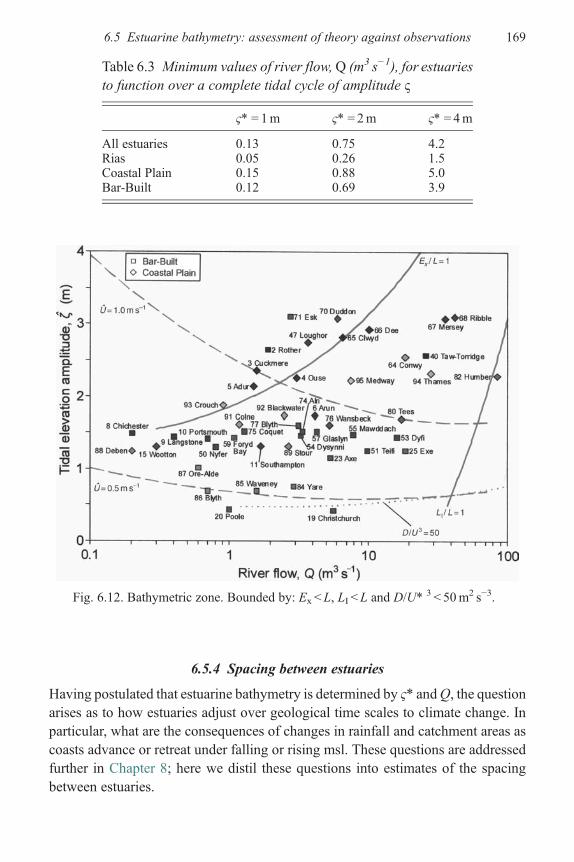
6.5.4 Spacing between estuaries

Having postulated that estuarine bathymetry is determined by ς* andQ, the questionarises as to how estuaries adjust over geological time scales to climate change. Inparticular, what are the consequences of changes in rainfall and catchment areas ascoasts advance or retreat under falling or rising msl. These questions are addressedfurther in Chapter 8; here we distil these questions into estimates of the spacingbetween estuaries.

Table 6.3 Minimum values of river flow,Q (m3 s−1), for estuariesto function over a complete tidal cycle of amplitude ς

ς* = 1m ς* = 2m ς* = 4m

All estuaries 0.13 0.75 4.2Rias 0.05 0.26 1.5Coastal Plain 0.15 0.88 5.0Bar-Built 0.12 0.69 3.9

Fig. 6.12. Bathymetric zone. Bounded by: Ex < L, LI < L and D/U* 3 < 50m2 s−3.

6.5 Estuarine bathymetry: assessment of theory against observations 169

For a long straight coastline with spacing, SP (km), between estuaries and arectangular catchment of landward extent CT (km), the river flow Q is given by

Q ¼ 0:032SP�CT�R; (6:29)

where R is the annual rainfall reaching the river (m a−1). Thus, typical UK values ofSP=10 km, CT= 50 km and Q= 15m3 s−1 indicate that R ~ 0.9m a−1, which is inbroad agreement with observations.By introducing (6.25) with tan α= 0.013 (Table 6.2), we obtain the following

expression for spacing between estuaries:

SP ¼ 41D5=2

R�CT: (6:30)

We note from Table 6.2 and from global observational data shown by Prandle(2004) that few estuaries have values of D > 20m. Hence, to avoid small valuesof SP for continental land masses with large values of CT, we anticipate theformation of deltas or multiple ‘sub-estuaries’ linked to the sea by tidal basinssuch as in Chesapeake Bay.

6.6 Summary of results and guidelines for application

By introducing the assumption of a ‘synchronous’ estuary (where the surface slopedue to the gradient in phase of tidal elevations significantly exceeds that fromchanges in amplitude ς*), explicit localised expressions are obtained for boththe amplitude and phase of tidal currents and the slope of the sea bed, SL, in termsof (D, ς*) where D is water depth. Integration of the expression for SL provides anestimate of the shape and length, L, of an estuary. By further combining these resultswith (4.44) for the length of saline intrusion, LI, an expression linking the depth at theestuarinemouth with river flow,Q, is derived, i.e. a morphological framework linkingthe size and shape of any estuary to river flow and tidal amplitude.

Recent attempts to forecast how estuarine bathymetries may evolve as a con-sequence of Global Climate Change have prompted the more fundamentalquestion:

What determines estuarine shape, length and depth?

Estuaries form an interface between the rise and fall of the tide at the coast and theriver discharges. Hence, we expect bathymetries must reflect a combination of tidalamplitude, ς*, and river flow, Q, alongside some representation of the alluvium.However, geological adjustment rates are extremely slow in comparison withthe (relatively) rapid changes in msl (and hence water depth) and Q. Thus, we

170 Synchronous estuaries

anticipate that bathymetries reflect some intermediate adjustment between ante-cedent formative conditions and subsequent present-day dynamic equilibrium.This adjustment rate will depend on both the supply of sediments for depositionand the ‘hardness’ of the geology for erosion.

Tidal currents and frictional influence

By introducing the ‘synchronous’ estuary assumption, Section 6.2 derives localisedexpressions, (6.8) and (6.9), for the amplitude and phase of tidal currents in termsof ς* and D, illustrating why U* is invariably in the range 0.5 <U* < 1.5m s−1

(Fig. 6.1). These synchronous solutions also explicitly quantify the issue raised inChapter 2 concerning the ratio of the frictional to inertial terms. Figure 6.3 showshow this ratio approximates 10 ζ* : D.

Lengths and shape

The expression (6.8) for the slope of the sea bed, SL, provides an estimate of theshape of an estuary (6.11). By subsequent integration of these slopes, Fig. 6.2 showsestuarine lengths, L (6.12), as a function of ς* andD and the bed friction coefficient,f, where the latter introduces some representation of the alluvium.

Range of estuarine morphologies

By combining these results for U* and L with the expression (6.16) for the lengthof saline intrusion, LI, a ‘bathymetric zone’ for ‘mixed’ estuaries is determinedenveloped by the conditions, LI/L< 1, Ex/L< 1 (Ex tidal excursion length) and theSimpson-Hunter (1974) criterion for vertical mixing (D/U*3< 50m−2 s3). Figures 6.5and 6.6 use the expression (6.9) for U* to indicate how the latter criterion fordetermining mixed versus stratified estuaries closely approximate the conditionς*� 1m.By introducing the observation that mixing occurs at a minimum in landward

intrusion of salt, an expression linking the depth at the mouth of an estuary D0 withriver flow, Q, is derived, (6.21) and (6.25). Interestingly, this expression is inde-pendent of both ς* and f. Assuming a triangular cross section with side slopes, tan α,between 0.02 and 0.002, Fig. 6.10 illustrates the resultant envelope of D0 as afunction of Q. This envelope supports the conclusion, derived in Chapter 4, that theriver flow velocity within the saline intrusion zone in mixed estuaries is invariablyof the order of (1 cm s−1).In Section 6.5, it is shown that for ‘mixed’ estuaries to function over the complete

tidal cycle requires minimum values of D ≈ ς*0.4 and Q ≈ 0.25m3 s−1. Typicalmaximum values of around D ≈ 20m and ς* ≈ 3m can be postulated and used tosuggest the formation of deltas and composite estuaries in the draining of largecontinental land masses.

6.6 Summary of results and guidelines for application 171

Assessment of bathymetric framework

Using the above relationship between D0 and Q, the earlier ‘bathymetric zone’ isconverted into a framework for estuarine morphology in terms of the ‘boundaryconditions’ ς* andQ, quantifying how tides and river flows determine estuarine sizeand shape. This framework, Fig. 6.12, is assessed against an observational data setextending to 80 UK estuaries.While individual estuaries exhibit localised features (related to underlying geol-

ogy, flora and fauna, historical development and ‘intervention’), the overall valuesof depth, length and (funnelling) shape are shown to be consistent with the newdynamical theories. Moreover, the morphological features which characterise Rias,Coastal Plain and Bar-Built estuaries can be rationalised by reference to thesetheories.The derived theoretical proportionality of L to D0

1.25 was substantiated for allthree estuarine types. For both Coastal Plain and Bar-Built estuaries, magnitudes ofL are in close agreement with the theory while Rias indicate significantly reducedvalues for L.Similarly, the theoretical proportionality of D0 to Q0.4 was substantiated for all

three estuarine types, with good magnitude agreement for Coastal Plain and Bar-Built estuaries while Rias indicated significantly larger values of D.

Theoretical Frameworks

Results derived in this chapter are synthesised into comprehensive TheoreticalFrameworks describing estuarine dynamics, salinity intrusion and bathymetry interms of the ‘natural’ boundary conditionsQ, ς* and f. The underlying relationshipsare as follows.

(a) Current amplitude U*∝ ς*½ D¼ f −½ Shallow water (6.9)∝ς* D−1/2 Deep water

(b) Estuarine length L∝D5/4/ς*½ f ½ (6.12)(c) Depth variation D(x)∝ x0.8 (6.11)(d) Depth at the mouth D0∝ (aQ)0.4 (6.25)(e) Ratio of friction: inertia F/ω∝ 10ς*/D (6.8)(f) Stratification limit D/U*3 ~ ς* = 1m (6.24)(g) Salinity intrusion Li,∝D2/fU0U* (6.16)(h) Bathymetric zone Bounded by LI < L, Ex < L

and D/U*3 < 50m−2 s3(6.23)

(i) Flushing time TF∝ LI/U0 (6.17)

These Frameworks provide perspectives against which to assess the morphologyof any particular estuary. By identifying ‘anomalous’ estuaries, possible causes canbe explored such as distinct regional patterns of historical evolution, engineer-ing ‘interventions’, ‘hard’ geology, dynamics or mixing inconsistent with the

172 Synchronous estuaries

theoretical assumptions, non-representative observational data, vagaries of sedi-ment supply and wave impact.The impact of flora and fauna has long been recognised as influencing the supply,

consolidation and bio-turbation of bed sediments. Section 6.2 shows how associatedvariations in the effective bed friction factor, f, have a major impact on dynamics andthence on both morphology and the sediment regime.

Corollary

The validation of these new theories provokes a paradigm shift, explored inChapter 7,suggesting that prevailing estuarine sediment regimes are the consequence of rather thanthe determinant for bathymetries.

References

Buck, A.L. and Davidson, N.C., 1997. An Inventory of UK Estuaries. Vol. 1.Introduction and Methodology. Joint Nature Conservancy Committee,Peterborough, UK.

Burgess, K.A., Balson, P., Dyer, K.R., Orford, J., and Townend, I.H., 2002. Futurecoastthe integration of knowledge to assess future coastal evolution at a national scale. In:28th International Conference on Coastal Engineering. American Society of CivilEngineering, Vol. 3, Cardiff, UK, pp. 3221–3233.

Davidson, N.C. and Buck, A.L., 1997. An inventory of UK estuaries. Vol. 1. Introductionand Methodology. Joint Nature Conservation Committee, Peterborough, UK.

Dyer, K.R., 1997. Estuaries: a Physical Introduction, 2nd ed. John Wiley, Hoboken, NJ.Friedrichs, C.T. and Aubrey, D.G., 1994. Tidal propagation in strongly convergent channels.

Journal of Geophysical Research, 99 (C2), 3321–3336.O’Brien, M.P., 1969. Equilibrium flow area of inlets and sandy coasts. Journal of

Waterways and Coastal Engineering Division ASCE, 95, 43–52.Prandle, D., 1985. On salinity regimes and the vertical structure of residual flows in narrow

tidal estuaries. Estuarine Coastal and Shelf Science, 20, 615–633.Prandle, D., 1997. The dynamics of suspended sediments in tidal waters. Journal of Coastal

Research, 25, 75–86.Prandle, D., 2003. Relationships between tidal dynamics and bathymetry in strongly

convergent estuaries. Journal of Physical Oceanography, 33 (12), 2738–2750.Prandle, D., 2004. How tides and river flows determine estuarine bathymetries. Progress in

Oceanography, 61, 1–26.Prandle, D., 2006. Dynamical controls on estuarine bathymetry: assessment against UK data

base. Estuarine Coastal and Shelf Science, 68 (1–2), 282–288.Prandle, D. and Rahman, M., 1980. Tidal response in estuaries. Journal of Physical

Oceanography, 70 (10), 1552–1573.Prandle, D., Lane, A., and Manning, A.J., 2006. New typologies for estuarine morphology.

Geomorphology, 81 (3–4), 309–315.Prandle, D., Lane, A., and Wolf, J., 2001. Holderness coastal erosion – Offshore movement

by tides and waves. In: Huntley, D.A., Leeks, G.J.J., and Walling, D.E. (eds),Land–Ocean Interaction, Measuring and Modelling Fluxes from River Basins toCoastal Seas. IWA publishing London, pp. 209–240.

References 173

Simpson, J.H. and Hunter, J.R., 1974. Fronts in the Irish Sea. Nature, 250, 404–406.Simpson, J.H., Brown, J., Matthews, J., and Allen, G., 1990. Tidal straining, density

currents and stirring in the control of estuarine stratification. Estuaries, 13 (2),125–132.

Schubel, J.R. and Hirschberg, D.J., 1982. The Chang Jiang (Yangtze) estuary: establishingits place in the community of estuaries. In: Kennedy, V.S. (ed.), EstuarineComparisons. Academic Press, New York, pp. 649–654.

174 Synchronous estuaries

7

Synchronous estuaries: sediment trappingand sorting – stable morphology

7.1 Introduction

Suspended sediments in estuaries generally increase upstream to produce a ‘turbid-ity maximum’ (TM) in the vicinity of the upstream limit of saline intrusion, withconcentrations hugely increased relative to open-sea conditions. Uncles et al. (2002)summarise observational studies of these TM and discuss mechanisms responsiblefor their formation. Here, for the case of strongly tidal estuaries, we develop genericquantitative expressions to represent the mechanisms producing these high sedi-ment concentrations. The aim is to identify the scaling parameters which determinethe sensitivities to sediment type (sand to clay), spring to neap tides and drought toflood river flows. Recognising the long-term stability of estuarine bathymetry,despite the continuous large ebb and flood sediment fluxes, an additional aim is toidentify feedback processes that maintain this stability.Postma (1967) first described the mechanisms responsible for estuarine trapping

of fine sediments, namely gravitational circulation, non-linearities in the tidaldynamics and delays between resuspension and settlement. However, these respec-tive roles are difficult to isolate either from observations or from models. Hence, ithas been difficult to gain a clear insight into the scaling of these processes and toestimate their sensitivities to changes in either marine or fluvial forcing or to internalparameters.

7.1.1 Earlier studies

Postma (1967) described the nature of sediment distributions in tidal estuaries andindicated likely controlling mechanisms. Salient characteristics identified byPostma include

(1) concentrations in suspension of fine sediments that are much higher than in relatedmarine or fluvial sources;

175

(2) provenance, both of suspended and of surficial bed sediments, is overwhelmingly ofmarine origin;

(3) evidence of lags between peaks in current and concentration, up to 4 days for the spring–neap cycle;

(4) lags that are associated with cumulative erosion and delayed settling for finer particles;(5) lags that are negligible for particles with diameters d ≥ 100 μm (settling velocity

Ws ≥ 0.01m s−1) and(6) peak suspended concentrations (TM) are widely observed, often related to the upstream

limit of gravitational circulation (saline intrusion) and with particle sizes typically100 > d > 8 μm.

Postma states that while estuaries may contain both coarse and fine material, it is thecharacteristics of the latter which generally predominate in determining bathymetryin conjunction with tidal amplitude, river flows and sediment supplies. Postma alsonotes the impacts of both flocculation and waves on sediment regimes. While theselatter impacts are widely acknowledged, the details of these processes are notconsidered here.Dronkers and Van de Kreeke (1986) observed that even in tidal bays with no

effective river flow, a landward increase in SPM is often observed. They showed howPostma’s (1967) concepts of ebb–flood asymmetry can be quantified to determine thenet transport of fine sediments.Festa and Hansen (1978), using a 2D laterally averaged model, indicated how

TM could be generated by gravitational circulation. Their study effectivelyassumed a rectangular cross section and involved tidally averaged dynamics.Using a steady-state numerical model with river flow UR = 0.02m s−1 (omittingboth erosion and deposition), they found that the strength and location of theTM depended critically on settling velocity, with pronounced TM for Ws >5 × 10−6 m s−1. Dyer and Evans (1989) incorporated sequential erosion anddeposition into a vertically averaged estuarine model and showed how the speci-fication of the erosion threshold influenced the balance of import and export ofsuspended sediments.The widely observed occurrence of TM close to the upstream limit of saline

intrusion led to assumptions that gravitational circulation was the generatingmechanism. Jay and Musiak (1994) emphasised the roles of both barotropic andbaroclinic mechanisms and the need to incorporate axial and vertical components ofthese in estimating net sediment fluxes. Jay and Kukulka (2003) quantified netresidual sediment fluxes associated with coupling between tidal variations in currentand SPM. They show how these fluxes can far exceed the fluxes derived from aproduct of net residual current and tidally averaged concentration. Their analysis issimilar to the present one, except that for partially stratified systems, baroclinicmodifications to tidal current profiles are more significant.

176 Synchronous estuaries

Markofsky et al. (1986) showed that the TM in the Weser traps silt, acting as afilter within the estuary. Utilising observed time series of suspended sediments inthe Weser, Grabemann and Krause (1989) showed that localised deposition andresuspension are dominant processes in the TM, with systematic repetition ofconditions over disparate cycles of tides and river flows. Lang et al. (1989) devel-oped a 3D numerical model to reproduce these observations, incorporating a settlingvelocity Ws = 5 × 10

–4m s−1. They suggested that some correlation might existbetween patterns of energy dissipation and source distributions of suspendedsediments.Hamblin (1989) indicated that local resuspension, ebb–flood asymmetry and

saline intrusion all contribute to TM in the St. Lawrence River. A model simulationspecified Ws = 3 × 10

−4m s −l, consistent with observed particle diameters in therange 10 < d < 20 μm.Uncles and Stephens (1989) describe extensive measurement of TM in the Tamar

River, where tidal range varies between 2 and 6m. They noted an order of magni-tude difference in TM concentrations over the spring–neap cycle. They also noted apreponderance of silt 20 < d < 40 μm, both suspended and deposited within the TMregion. They suggested that resuspension, tidal pumping and gravitational circula-tion may all be contributing mechanisms. The authors also note the importance offlocculation of fine sediments in suspension and of the rapid change in density/porosity of recently deposited sediments.In a subsequent investigation of TM in the Tamar River, Friedrichs et al.

(1998) determined that TM were primarily linked to internally generatednon-linearities with three dominant effects: (i) flood-dominant asymmetry, (ii)river flow and (iii) settling lag effected via breadth convergence. Conversely,axial variations in depth were not found to be important. An axially varying bederodability was found to be necessary to maintain an overall sediment budget.Their model introduces a time lag between peaks in current speed and concen-tration of 45min.Aubrey (1986) emphasised the role of tidal distortions associated with

channel geometry and bed friction in producing flood or ebb dominance inshallow estuaries. Aubrey noted the dependence of the magnitude of these distor-tions on ς*/D. Here, we concentrate on estuaries with large tidal amplitude–depth ratios in shallow, triangular cross sections with associated strong verticalmixing.

7.1.2 Approach

The present approach involves direct integration of expressions for tidaldynamics, salinity intrusion and sediment motions into an analytical emulator.

7.1 Introduction 177

The emulator is applicable within strongly tidal (hence mixed) funnel-shapedestuaries and incorporates processes that are pronounced in shallow estuarieswith triangular cross sections. It provides clear illustrations of parameter depen-dencies and enables conditions of zero net sediment flux to be determined. Whilethese results are, to some degree, dependent on a priori assumptions, the approachhas the advantage of (i) relatively straightforward mathematics, (ii) genericapplication over a wide range of parameters, namely tidal elevation amplitudeς*, water depth D, river flow Q, sediment type or fall velocity Ws and frictioncoefficient f.The primary objective is to integrate into an ‘analytical emulator’ simplified

descriptions of the salient mechanisms of

(1) tidal and residual currents associated with saline intrusion, river flow and tidal non-linearities;

(2) sediment erosion, suspension and deposition

to produce expressions for mean concentrations and net cross-sectional fluxesof SPM.Section 7.2 summarises results for (1) as described previously in Chapters 4

and 6. Similarly, Section 7.3 summarises results for (2 ), based on Chapter 5 ,introducing continuous functional representations (7.22) for the half-life of sedi-ments in suspension, t50, and for their vertical profile e

−βz, (7.24). In Section 7.4, thevalidity of the resulting expressions for sediment concentrations and net fluxes areassessed against numerical model simulations (Fig. 7.1; Prandle, 2004c).Section 7.5 examines component contributions to net sediment flux with atten-

dant sensitivity analyses. It is shown how separate current components fromthe tidal non-linearities, involving cos θ and sin θ, largely determine the balancebetween import and export, where θ is the phase difference between tidal elevation,ς* and current, U*. The combinations of parameter values which produce zero netsediment fluxes are then determined.Section 7.6 summarises these earlier results indicating in Fig. 7.8 how, for fall

velocities of 0.0001, 0.001 and 0.01m s−1, the balance between net import orexport changes as tidal amplitudes vary from 1 to 4m (indicative of neap to springvariations). Proceeding upstream from deep to shallow water, the balance betweenimport of fine sediments and export of coarser ones becomes finer, i.e. selective‘sorting’ and trapping. Likewise, more imports, extending to a coarser fraction,occur on spring than on neap tides.In Section 7.7, the above results are encapsulated into new estuarine typology

framework (Figs 7.9–7.11) comparing observed versus theoretical dynamics, bathy-metry and sediment regimes for a wide range of estuaries.

178 Synchronous estuaries

7.2 Tidal dynamics, saline intrusion and river flow

Estuarine dynamics are largely determined by tides and estuarine bathymetry withsome modulation by river flow evident close to the tidal limit. For the case of asynchronous estuary, Chapter 6 presents localised solutions for the amplitude andphase of tidal currents expressed in terms of tidal elevation amplitude and waterdepth. For completeness, these solutions are summarised here. Similarly, the salientfeatures of the dynamics associated with saline intrusion and river flow, described inChapter 4, are summarised.These solutions apply to the case of a single (predominant) tidal constituent in a

triangular-shaped estuary. Convective and density gradient terms are neglected, and

0.05(a) Sand

Silt

Clay

1

10

100

400

0.005

0.0005

D(m)

4 8 16

Ws(m s–1)

(b)–10

–100

–500

0

500

1000

0.05 Sand

Silt

Clay

0.005

0.0005

D(m)

4 8 16

Ws(m s–1)

(c)

–10

–100

–500

0

1000

0.05 Sand

Silt

Clay

0.005

0.0005

D(m)

4 8 16

Ws(m s–1)

Fig. 7.1. Analytical Emulator versus Numerical Model values of suspendedconcentrations and net fluxes.Model (solid contour), analytical emulator (7.29a) (dashed);(a) Depth- and time-averaged concentrations (mg l−1),(b) net depth-integrated sediment fluxes from the numerical model;(c) net depth-integrated sediment fluxes from the analytical emulator (7.31).Values are for ζ*= 2m and f=0.0025. Fluxes are in tm−1 width per year, positivelandward.

7.2 Tidal dynamics, saline intrusion and river flow 179

the friction term is linearised. It can be shown (Prandle, 2004b) that tidal propaga-tion in ‘mixed’ estuaries is almost entirely unaffected by saline intrusion.

7.2.1 Analytical solution for 1D tidal propagation(Chapter 6; Prandle, 2003)

Omitting the convective term from the momentum equation, we can describe tidalpropagation in an estuary by

@U

@tþ g

@&

@Xþ f

UjUjH

¼ 0 (7:1)

B@B@t

þ @

@XAU ¼ 0; (7:2)

where U is velocity in the X direction, ς is water level, D is water depth, H is thetotal water depth (H=D+ ς), f is the bed friction coefficient (~0.0025), B is thechannel breadth, A is the cross-sectional area, g is gravitational acceleration and t istime.Concentrating on the propagation of one predominant tidal constituent, M2, the

solutions for U and ς at any location can be expressed as

& ¼ &� cos ðK1 X� ω tÞ (7:3)

U ¼ U� cos ðK2X� ω tþ θÞ; (7:4)

where K1 and K2 are the wave numbers, ω is the tidal frequency and θ the phase lagof U* relative to ς*.Further assuming a triangular cross section with constant side slopes, where

U∂A/∂X≫ ∂U/∂X and ∂D/∂X≫ ∂ς/∂X, we simplify the continuity equation to

@&

@tþU

@D

@XþD

2

@U

@X¼ 0: (7:5)

The component of f U|U|/H at the predominant tidal frequency M2 may be approxi-mated by (Prandle, 2004a):

8

3π25

16fjU�jUD

¼ FU; (7:6)

with F= 1.33 f U*/D. By specifying the synchronous estuary condition thatthe spatial gradient in tidal elevation amplitude is zero, we derive K1 =K2 = k,i.e. identical wave numbers for axial propagation of ς and U. Thus,

tan θ ¼ F

ω¼ � SL

0:5 D K(7:7)

180 Synchronous estuaries

U� ¼ &�g k

ðω2 þ F2Þ1=2; (7:8)

where SL= ∂D/∂X, and

k ¼ ω

ð0:5DgÞ1=2: (7:9)

Thus, in shallow water, values of U* are proportional to D1/4(ς*/f )1/2 and tan θ isproportional to D−3/4(ς* f)1/2.

7.2.2 Saline intrusion (Chapter 4)

For the case of a well-mixed estuary with a constant axial salinity gradient, Sx, thefollowing expression for residual velocities associated with saline intrusion, Us, atfractional height z (=Z/D) above the bed was derived using (4.15), Prandle (1985):

Us ¼ g SxD3

Kz

�z3

6þ 0:269z2 � 0:0373z� 0:0293

� �; (7:10)

where Kz is the vertical eddy diffusivity.For well-mixed conditions, the length of saline intrusion LI is given by (4.44):

LI ¼ 0:005 D

f U� UR

; (7:11)

where UR is the residual velocity component associated with river flow and Sx maybe approximated by the ‘relative’ salinity gradient:

Sx ¼ 0:027

LI

: (7:12)

Here we assume that the eddy diffusivity coefficient equals the eddy viscositycoefficient and is given by

KZ ¼ E ¼ f U� D: (7:13)

Then from (7.10), (7.11), (7.12) and (7.13), we estimate Us at the bed as

US ¼ �1:55UR; (7:14)

independent of f,U* orD. Moreover, it was shown in Chapter 5 thatUR is generallyorder of (1 cm s−1); hence, we anticipate values of residual currents associated withan axial salinity gradient of typically 1 or 2 cm s−1. Prandle (2004b) showed that theneglect of convective overturning in deriving (7.10) results in an underestimation ofUs by a factor of up to 2. Figures 6.4 and 6.5 (Prandle, 2004a) show that for a

7.2 Tidal dynamics, saline intrusion and river flow 181

synchronous estuary, stratification is generally confined to ς* < 1m. However, someelement of intra-tidal stratificationwill occur for larger values of ς*. Such stratificationcan significantly increase values of Us; for example, Dronkers and Van de Kreeke(1986) show values of Us up to 10 cms−1 in the partially stratified Volkerak estuary.

7.2.3 River flow

Equation (4.12) provides the following approximation for the vertical profile ofriver flow in a strongly tidal estuary:

UR ¼ 0:89 �UR � z2

2þ zþ π

4

� �: (7:15)

7.3 Sediment dynamics

Chapter 5 describes localised solutions for suspended sediment concentrations.These are summarised here prior to incorporation alongside synchronous estuarysolutions in Section 7.4.

7.3.1 Suspension, erosion, deposition and vertical profiles

Neglecting horizontal components of advection and dispersion, a localised distribu-tion of suspended sediments can be described by the dispersion equation

@C

@t�WS

@C

@Z¼ KZ

@2C

@Z2� Sk þ Sc; (7:16)

where Sk and Sc are sinks and sources of sediment. Following Prandle (1997a and1997b), we assume sediment concentration time series associated with each ero-sional event of magnitude M, (5.11):

CðZ; tÞ ¼ M

ð4πKztÞ1=2exp�ðZþWstÞ2

4Kztþ exp�ð2DþWst� ZÞ2

4Kzt

" #: (7:17)

This assumes deposition at the bed both by advection and dispersion for particlesthat return to the bed following ‘reflection’ at the surface. An observed time seriesrepresents a time integration of all such preceding ‘events’.

Erosion

Erosion ER(t), due to a tidal current U(t), is assumed to be of the form

ERðtÞ ¼ fγ ρ Uj jN; (7:18)

182 Synchronous estuaries

where N is some power of velocity typically in the range of 2–5 and ρ is waterdensity. For N= 2, Prandle et al. (2001) derived γ= 0.0001m−1 s; for convenience,this formulation is adopted here. This implies a rate of erosion directly proportionalto frictional bed stress.

Deposition

Chapter 5 describes solutions of (7.16), showing that deposition can be approxi-mated by an exponential function e−αtwith ‘half-life’ t50 = 0.693/α, where α is givenby the larger of (5.14) and (5.15), i.e.

α ¼ 0:693W2

s

KZ

(7:19)

α ¼ 0:1Kz

D2: (7:20)

The parameter Kz/WsD, which characterises the governing mechanics, is inver-sely proportional to the familiar Rouse number. It is shown in Chapter 5 thatmaximum half-lives occur at Kz/Ws D= 2.5. For Kz/WsD≫ 1, dispersion predomi-nates, and sediments are well mixed vertically. Conversely, for Kz/WsD≪ 1, advec-tive settling predominates, and sediments remain close to the bed. Figure 5.4 showsthe relationship betweenWs and Kz/WsD for a range of values of ς* (utilising (7.8)and (7.13)). This illustrates how the demarcation line ofKz/WsD ~ 1 coincides withfall velocities of order of (1mm s−1) or, for

Wsðms�1Þ ¼ 10�6 d 2ðμÞ (7:21)

a particle diameter d of order of (30 μm). It is shown in Section 7.5 that the sedimentbalance in estuaries is especially sensitive to sediments in this range.To construct an analytical emulator, we need a continuous transition between

conditions (7.19) and (7.20). By simple curve fitting, the results shown in Fig. 5.2can be closely approximated by (5.17):

α ¼ 0:693Ws=D

10x; (7:22)

where x is the root of the equation

x2 � 0:79xþ jð0:79� jÞ � 0:144 ¼ 0 (7:23)

with j = log10 Kz/WsD.

Vertical profile of suspended sediments

In subsequent estimates of net tidal fluxes, continuous functional descriptions of thevertical profiles of suspended sediment concentrations are required. By numerical

7.3 Sediment dynamics 183

fitting of a profile e−βz to simulations based on (7.17), the following expression for βwas derived using (5.19):

β¼ 0:91 log10 6:3Kz

WsD

� �� ��1:7

� 1: (7:24)

Figure 5.5 shows, for a range of values of Kz/WsD, values of β from (7.24)alongside related sediment profiles. These results illustrate how effective com-plete vertical mixing is achieved for Kz/WsD > 2, and ‘bed load’ only occurs forKz/Ws D < 0.1.

7.4 Analytical emulator for sediment concentrations and fluxes

Here, the dynamical results described in Section 7.2 are integrated with the sedimentsolutions from Section 7.3 to form an ‘analytical emulator’ for determining netsediment fluxes (Prandle, 2004c). Erosion, assumed proportional to velocitysquared, is modulated by an exponential settling rate to yield mean and tidallyvarying components of sediment concentration. The approach assumes that contin-uous cyclical erosion and deposition coexist without threshold values. Figure 7.7summarises how these flux components are determined from the product of tidaland residual velocities (modified for vertical structure components) with theseconstituents of sediment concentration (likewise modified for vertical structure).

7.4.1 Erosional velocity components

Section 2.6.3 shows that to maintain continuity in a tidally varying cross sectionwhere net flux isU1 times the mean cross-sectional area, theM2 currentU1* cos (ωt)given by (7.4) must be accompanied by both M4 and Z0 (residual) components:

U�2 ¼ �aU�

1 cos 2ωt� θð Þ½ �U0

0 ¼ �aU�1 cos θ;

(7:25)

where a= ς*/D for a triangular channel and a= 0.5 ς*/D for a rectangular channel.

Mean concentration

Henceforth for clarity of other symbols, the asterisks used to designate tidalamplitudes, ς* and U*, are omitted.Assuming erosion is proportional to velocity V squared, the expansion of M2, M4

and Z0 velocity constituents gives

V2 ¼ ½U1 cosωtþU2 cos ð2ωt� θÞ þU0�2; (7:26)

184 Synchronous estuaries

where U0 = U00 + UR + Us, with U2 and U0

0 from (7.25) and UR and Us from (7.15)and (7.10), respectively. This yields suspended mass components at the followingtidal frequencies (scaled by fγρ from (7.18)):

ðU1 cosωtþU2 cosð2ωt� θÞ þU0Þ2 ¼ V20 þ V2

ω þ V22ω þ V2

3ω þ V24ω

with V20 ¼ 0:5ðU2

1 þU22Þ þU2

0

V2ω ¼ U1U2 cos ðωt� θÞ þ 2U0U1 cosωt

V22ω¼ 2U0U2 cos ð2ωt� θÞ þ 0:5U2

1 cos 2ωt

V23ω¼ U1U2 cos ð3ωt� θÞ

V24ω¼ 0:5U2

2 cos ð4ωt� 2θÞ:

(7:27)

7.4.2 Mass of sediments in suspension

From Section 5.5, the mass in suspension for each cyclical erosion component atfrequency ω, when modulated by deposition at the rate e− αt, is given by (5.20):

CðtÞ ¼ðt

�1cosωt0e�αðt�t0Þ dt0 ¼ α cosωtþ ω sinωt

α2 þ ω2; (7:28)

where the integral sums backward in time to represent all remaining contributions tosuspended concentration.Thus, (7.28) modulates the erosion at any frequency to yield a concentration

proportional to 1/(α2 + ω2)1/2. From (7.27), (7.28) and (7.18), we note that the netmass in suspension includes components at frequencies σ as follows:

σ ¼ 0; massMCI CD ¼ fγρU2

0 þ 0:5 U21 þU2

2

� �� α

(7:29a)

σ ¼ ω; mass MC2 CD ¼ fγρU1U2

α2 þ ω2½α cosðωt�θÞ þ ω sinðωt�θÞ� (7:29b)

σ ¼ ω; mass MC3 CD ¼ fγρ2 U0 U2

α2 þ ω2½α cosωtþ ω sinωt�: (7:29c)

Additional components can be shown not to contribute to net sediment flux and,hence, are omitted in (7.29).Figure 7.1a (Prandle, 2004c) shows the correspondingmean concentrations obtained

from (i) a cyclical tidal numerical model simulation of (7.17) and (ii) the σ=0 compo-nen t of (7 .29) . Goo d agr eement i s s hown ov er a ra nge of va lues o f both Ws andD. Theseresults are for ς*=2m, f=0.0025 and UR=0.01ms−1, with U1 calculated from (7.8).

7.4 Analytical emulator for sediment concentrations and fluxes 185

The full concentration time series can be calculated by summing each of thecomponents, σ= 0, ω to 4ω, in (7.27) with their modulation by deposition at therate e−αt as indicated in (7.28).

7.4.3 Net sediment fluxes

Sediment fluxes involve the product of erosion, from (7.27), modulated bydeposition, via (7.28), multiplied by the velocity component appropriate to an(assumed) constant depth i.e. U1 cosωt + URS, where URS =UR + US. The verticalstructure of concentrations is approximated by e−βz, with β estimated from (7.24).The resulting concentration time series can be calculated by summing each of thefive components in (7.27) together with their modulation by deposition at the ratee−αt (Section 7.3).The vertical structure of the velocity components associated with salinity intru-

sion and river flow are specified from (7.10) and (7.15), respectively. The verticalstructure for the M2 tidal constituent is approximated by

UðzÞ ¼ �U 0:7þ 0:9 z� 0:45 z2� �

; (7:30)

where �U is the depth-averaged tidal velocity amplitude.No account of vertical phase variations is considered. For the M4 constituent,

it can be shown that only the ratio of bed to depth mean value is required; forsimplicity, a uniform vertical structure is assumed.The parameters U1, U2 and U0, describing erosion in (7.26), represent velocities

at the bed. We introduce the coefficients P and Q to represent depth variations(relative to the bed) in U1 and URS, respectively. From (7.30) the value of P ~ 1/0.7,while from (7.14) and (7.15)Q ~ 1/− 0.69. Net sediment fluxes are then obtained bymultiplying the erosional components (7.27), modulated via the suspension expres-sion (7.28), and the vertical profile (7.24) by the velocity component (PU1 cosωt +QURS). The latter is consistent with the assumption of a net semi-diurnal waterflux plus river and salinity components. This yields residual sediment fluxes (F) asfollows:

F1 ¼ 1

αQ URS U2

0 þ 0:5 ðU21 þU2

2Þ�

(7:31a)

for mass MC1 and flow QURS.

F2 ¼ 1

α2 þ ω2P U2

1 U2 ð0:5 α cos θ�0:5 ω sin θÞ (7:31b)

for mass MC2 and flow PU1 cosωt.

186 Synchronous estuaries

F3 ¼ 1

α2 þ ω2P U2

1 U0 α (7:31c)

for mass MC3 and flow PU1 cosωt.For (7.31), flux magnitudes are again scaled by fγρ, and concentrations are

modulated by the vertical structure of the concentration βe−βz/(l − e−β).The first component, Fl (mass component MC1), represents the flux associated

with the product of (i) time-averaged SPM concentration, MC1 in (7.29), and(ii) residual currents associated with river flow and saline intrusion. The secondcomponent, F2 (mass component MC2), results from (iii) the semi-diurnal SPMcomponent generated by the combination ofU1 cosωt andU2 cos (2ωt− θ) in (7.26)advected by (iv) the semi-diurnal current U1 cosωt. The first (cos θ) part of theresulting flux may be interpreted as representing the downstream (U2 is negativefrom (7.25)) export of coarser (large α) sediments. Equivalently, the secondpart (sin θ) represents upstream import of finer sediments (small α). The thirdcomponent, F3 (mass component MC3), is similar to the second, except thatthe semi-diurnal SPM component (v) arises from the combination of U0 andU1 cosωt in (7.26), i.e. MC3 in (7.29). Since U0 ~U 0

0 ~U2 cos θ, this third fluxcomponent effectively increases the (cos θ) term in component (ii) by a factor of 3(see Section 7.5).Depth-integrated fluxes, corresponding to the conditions for Fig. 7.1(a), are

shown (i) in Fig. 7.1(b) for a cyclical tidal numerical simulation and (ii) inFig. 7.1(c) for the above analytical expansion (7.31). For these fluxes, agreementis not as close as for concentrations. However, the essential patterns and generalmagnitudes are sufficiently similar to warrant adoption of the analytical emulator forsubsequent analyses of the characteristics and sensitivities of net sediment fluxes intidal estuaries.Figure 7.1(b) and (c) shows maximum upstream sediment fluxes exceeding

1000 tm−1 width per year occurring for the finest sediment in the shallowest water.This value reduces for coarser material and in deeper water, reversing direction forWs > 0.002m s−1, with maximum downstream flux forWs ~ 0.005m s−1. By compar-ison, estimates of sediment deposition in the Mersey River over the last centuryinvolve net sediment fluxes of order of (1000 t year−1m−1) (Lane, 2004).

7.5 Component contributions to net sediment flux

Having demonstrated the validity of the analytical emulator in Section 7.4, we nowapply the emulator to examine the component contributions to net sediment fluxesand, specifically, to identify conditions consistent with zero net fluxes, i.e. bathy-metric stability.

7.5 Component contributions to net sediment flux 187

7.5.1 Components of sediment flux: river flow, salinity and tidalcurrent constituents

We note, from Section 7.2, that the components of residual velocities UR and Us

associated with both river flow and salinity are typically two orders of magnitudeless than U1. Prandle (2003) calculated, for a random selection of 25 UK estuaries,an average value on extreme spring tides of a= ς/D= 2/3. Then from (7.25), weestimate that the components ofU0 andU2 related to varying estuarine cross sectionare typically as follows: (i) for U2, comparable but less than U1 and (ii) for U0, anorder of magnitude less than U1.For ς* = 2m and f= 0.0025, Fig. 7.2(a) and (b) (Prandle, 2004c) shows residual

sediment fluxes associated with (i) river flow UR =− 0.01m s−1 and (ii) salinityvelocity US from (7.10). River flow produces net downstream fluxes whichincrease with greater water depths and with finer sediments. Saline intrusionproduces upstream fluxes increasing with greater depths and shows a maximumfor Ws ~ 0.002 m s− 1 . We s ee tha t the n et f luxes ass oci ate d with F1 in (7.31) ar esignificantly less than for F2 and F3.Figure 7.2(c) and (d) shows net fluxes associated with the the tidal coupling

terms, F2 and F3. The relative magnitude of these coupling terms is directly related

0.05(a) (c)

(d)(b)

–10

1010

100

1000

3000

100

250

–10

–100–1000

–2000

–100

–500

0.005

0.0005

4 8 16

D(m)

Ws(m s–1)

0.05

0.005

0.0005

Ws(m s–1)

4 8 16

D(m)

Fig. 7.2. Components of net depth-integrated sediment flux from (7.31).(a) F1, river flow UR=− 0.01m s−1;(b) F1, saline intrusion velocities, (7.10);(c) cosine terms in components F2 and F3 of (7.31);(d) sine terms in component F2.Conditions, conventions and units as for Fig. 7.1.

188 Synchronous estuaries

to the phase difference θ between M2 tidal elevation and current. The generalnature of this balance between the ‘cosine’ and ‘sine’ terms is shown in Fig. 7.3over a range of values of half-life in suspension, t50, and θ. Their contributions varyin a complex fashion given the counteracting sensitivities of U1 and θ to changes indepth, (7.7) and (7.8). Likewise, their sensitivity to half-lives in suspension, t50(or Ws), is reflected in the dependence of the cosine and sine terms on α/(α2 +ω2)andω/(α2 +ω2), respectively. Combining the sensitivities of these terms in (7.31) toboth α and θ, we anticipate that for the finest sediment in shallow water (θ →90°),the sin θ term will predominate, while for coarser sediments in deeper waters(θ→0°), the cos θ term will predominate.From (7.31), assuming the term involving U1 predominates in F1 and that

U0 ~U 00 =− aU1 cos θ, then the ratio of F1 to F2 + F3 terms can be simplified to

0:5 U21 URS=α

0:5 aU31 ð3 α cos θ�ω sin θÞ=ðα2 þ ω2Þ (7:32)

(neglecting the parameters Q and P and the effect of vertical profiles in concentra-tion); noting that URS ~− 0.01m s−1and letting r=ω/α, (7.32), simplifies to

�0:01

�aU1

3 cos θ1þ r2

� r sin θ1þ r2

�� : (7:33)

–0.01–0.5

–1

–2

–3(a)

100

1

0.01

t50(h)

0.50.25

0.1

0.01(b)

90° 60° 30° 0°90° 60° 30° 0°

90°

0.1

0.5

–0.1 –1 –2–3

0

100

1

0.01(c)

t50(h)

60° 30° 0°θ

θ θ

Fig.7.3. Values of net import (+ve) and export terms in (7.31) as f ( θ, t50). (a) Cosineterms, (b) sine term and (c) summation of (a) and (b).

7.5 Component contributions to net sediment flux 189

Figure 7.3(a) (Prandle, 2004c) represents (−3 cos θ)/(l + r2), Fig. 7.3(b) represents(r sin θ)/(l + r2) and Fig. 7.3(c) represents the summation of these.We note that theseterms balance in the region 1< t50 < 10 h when t50 ~ 10(1− θ/90) h. Further descrip-tion of the significance of the parameter r follows in Section 7.7.

7.5.2 Conditions for zero net flux of sediments

To convert from the generalised scaling results shown above to more specific estuarineconditions, we adopt the dynamical solutions for synchronous estuaries. This enablesresults to be presented in termsof the immediately familiar parameters, ς* (tidal elevationamplitude) andD (water depth), pertaining at any selected section of such estuaries.Then for any combination of (D, ς*), by scanning across a range of settling

velocities, Ws, a balance between the predominant landward and the seaward tidalcoupling terms in (7.33) can be found. Figure 7.4 (Prandle, 2004c) shows these ‘zeroflux’ values for a (i) half-life t50; (ii) particle diameter d, (7.21); (iii) fall velocity Ws,(7.22) and (iv) mean concentration, (7.29). The indicated range of values for particlediameter, 30< d <50μm, is reasonably consistent with results described in Section7.1.1 fromPostma (1967), Uncles and Stephens (1989) andHamblin (1989). Likewise,the range of values for settling velocity, 1 <Ws < 2.5mm s−1, is close to the value

4

(a) (c)

(d)(b)

3

2

1

0

1.5

1.0

2.02.5

4

3

2

1

04 8

D(m)

ζ(m)^

ζ(m)^

D(m)16 32

30

40

200

0.51

2 3

100

4 8 16 32

150 20050

Fig. 7.4. Conditions for zero net sediment flux as f(D, ς*), with U0 = − 0.01m s−1

and f = 0.0025.(a) Half-life t50 (h),(b) particle diameter (μm),(c) fall velocity Ws (mm s−1) and(d) mean sediment concentration (mg l−1).

190 Synchronous estuaries

adopted for the Weser River by Lang et al. (1989). Moreover, there is recentevidence (Manning, 2004) from a number of estuaries of predominant settlement,via flocculation, at values of Ws ~ 1mm s−1. The mean depth and tidally averagedsuspended concentrations, 50 <C < 200mg l−1, are within the lower range ofobserved maximum concentrations, 10–10 000mg l−1, found in TM (Uncleset al., 2002). However, these estimates may be substantially increased byvariations in the effective friction coefficient, here taken as f = 0.0025. An inter-esting feature of these results is the near constancy of the parameter Kz/Ws D ~ 1.6throughout the range of (D, ς*). It was noted earlier that maximum half-livescorrespond to Kz/Ws D = 2.5, which coincides with Ws ~ 1mm s −1. This indicatesthe coexistence of maximum concentrations with conditions of morphologicalstability.

7.5.3 Sensitivity to fall velocity, Ws

Figure 7.5(a) and (b) shows net sediment fluxes and mean suspended concentra-tions, calculated from (7.31) and (7.26), for the values Ws = 1 and 2mm s−1,suggested from Fig. 7.4(c) to be consistent with stable morphology. For the finermaterial, net fluxes are upstream for all but the lowest tides and deepest water.Moreover, these upstream fluxes increase roughly in proportion to ς3. Conversely,

4

(a) (b)

3

2

1

0

0

4 8 16 4 8 16

10

50

100

150 200

–100

–500

–100

0 10002000

D(m) D(m)

–100

1000

10,000

500400

250

100

5000

ζ(m)^

4

3

2

1

0

ζ(m)^

3000

Fig. 7.5. Sediment fluxes (top) in t year−1m−1 and concentrations (bottom)in mg l−1 as f(D, ς*). (a) Left, WS = 0.001m s−1 and (b) right, WS= 0.002m s−1.D depth, ς tidal elevation amplitude.

7.5 Component contributions to net sediment flux 191

for the coarser material, net fluxes are downstream for all but the largest tides anddeepest water. These results clearly illustrate how both the direction and themagnitude of the net sediment fluxes can vary abruptly between spring and neaptides, from mouth to head, and for different sediment sizes.

7.5.4 Sensitivity to bed friction, f , and fall velocity, Ws

Corresponding calculations were made for the component contributions to thesenet fluxes. However, the scaling of the components shows less variation with eitherς or D than for variations inWs and the bed frictional coefficient f. To illustrate this,

Fig. 7.6. Sensitivity of dynamics, sediment concentrations and net fluxes to fallvelocityWS and friction factor f. Results for ς* = 3m and D= 8m.(a)–(c). Percentage of net sediment flux in (7.31).(a) F1,(b) cosine flux term in F2 and F3,(c) sine term in F2,(d) tidal velocity U* and phase θ,(e) net flux Fl + F2 + F3 (t year−1 m−1),(f) concentrations (mg l−1) and(g) half-life t50 (h).

192 Synchronous estuaries

Fig. 7.6 (Prandle, 2004c) shows, for the case of ς = 3m and D= 8m, these propor-tional components (in percentages) associated with (a) URS (b) cos θ and (c) sin θ in(7.33) for 0.0005 <Ws < 0.05m s−1 and 0.0005 < f< 0.0125. These results show,consistent with Figs 7.4 and 7.5 and (7.28), that the cosine term predominatesoverall, producing a maximum (proportional) seaward flux for coarse sedimentsover the smoothest beds. Conversely, the sine term produces net upstream fluxesfor the finest sediments over the roughest beds. Both of these results emphasise thereinforcement of axial sediment sorting noted in Section 7.5. By contrast, the role ofthe river and saline velocity components is generally negligible in all but the deepestwaters. Moreover, while the salinity component predominates over the riverinecomponent in transporting (near-bed) coarser material landward, the opposite occursfor (more uniformly distributed) finer sediments.The significant sensitivity of both U* and θ to changes in bed friction is evident in

Fig. 7.6(d)with consequent influences on concentrations and fluxes. Figure 7.6(e)–(g)indicates the related sensitivities of net flux, mean concentration and half-life insuspension.

7.6 Import or export of sediments?

This section summarises and interprets the application of earlier results for zero netsediment fluxes. Figure 7.7 presents a schematic of the dynamical and sedimentarycomponents integrated into the analytical emulator used above to derive conditionscorresponding to zero net flux of sediments, i.e. stable bathymetry.

Fig. 7.7. Dynamical and sedimentary components integrated into the analyticalemulator.

7.6 Import or export of sediments? 193

7.6.1 Sensitivity to half-life, t50, and phase difference, θ,between tidal elevation and current

The sensitivity of conditions corresponding to zero net flux of sediments areillustrated in Fig. 7.8 for (i) changes in sediment size, (ii) over the length of anestuary (indicated by changing depths) and (iii) over the spring–neap tidal cycle. Nettransports of fine sediments are quantified in (7.33) and illustrated in Fig. 7.3(c). InFig. 7.8 (Prandle et al., 2005), loci of spring–neap variations for tidal elevationamplitudes ς = 1, 2, 3 and 4m are superimposed onto these results. These loci are fordepthsD= 4 and 16m and for fall velocitiesWS = 0.01, 0.001 and 0.0001m s−1. Thevalues for θ are from (7.7) adopting the assumption for bed friction coefficientf= 0.001 (d/10)½, where d is particle diameter in micrometre and (7.21) relatesWS tod. Corresponding values for t50 are from (7.22).Progressing from neap to spring tides increases (the absolute value of) θ and

hence reduces the export or increases the import of sediments. This same trend isfound in shallower depths, emphasising how estuaries can trap sediments inupstream sections. However, as more finer sediments are trapped, the effectivevalue of f decreases, resulting, (6.12), in a tendency to increase estuarine length.Hence, some equilibriumwill prevail, governed by the balance between the type and

–90° –45° 0°100

1

0.010.1 0.5 0.9 0.99

0

–0.01

–0.1

Import

Exp ort

–0.5

Sand

Silt

10

0.1

4 m

16 m

4 m

16 m

4 m

= 4 3 2 1 m T idal amplitude ζ̂

Ws = 0.01 0.001 0.0001 m s�1

16 m

Hal

f life

t 50

(h)

Phase advance, θ, of ζ with respect to Ûˆ

Fig. 7.8. Spring–neap variability in net import versus export of sediments (7.33), asa f (t50, θ). Variability over elevation amplitude ς* = 1, 2, 3 and 4m, fall velocitiesWS= 0.0001, 0.001 and 0.01m s−1 for depths D = 4 and 16m.

194 Synchronous estuaries

the quantity of (marine) sediment supply, enhanced trapping of fine sediments andconsequent more energetic dynamics attempting to increase depths.From Fig. 5.2, for Kz/WsD< 2, we can approximate α=Ws

2/Kz, i.e.r=ω/α= 3.5 × 10−7U*D/Ws

2. For typical values of U* ~ 1m s−1 and D ~ 10m,then r < 1 for Ws > 2 × 10−3 m s−1. Hence from (7.33), river flow and associatedsalinity intrusion (involving velocities of a few centimetres per second) will havelittle impact for sediments coarser than the above and as long as (aU*)≫ 0.01m s−1,i.e. a= ς /D≫ 0.01 (for the M2 constituent).Within these regions where tidal influences predominate, the ratio of sediment

import (IM) to export (EX) is given by the denominator terms in brackets in (7.33):

IM

EX¼ r

3tan θ ¼ 0:4

f U�

Ws

� �2(7:34)

on the basis of the above approximation for α and substituting for tan θ from (7.7).Zero net flux then corresponds to

Ws ¼ 0:6 f U�� 0:0015 U� (7:35)

(for f = 0.0025). This estimate forWs is in close agreement with the values shown inFig. 7.4(c).The distribution for mean sediment concentration may be approximated by

inserting Ws from (7.35) in (7.29), neglecting U0 and using the above values forα, thus

C ¼ γ ρ f U�2=Dα � γ ρ U�ð1þ a2Þ: (7:36)

Noting, as indicated in Section 7.2, that in shallow water, U* is proportional to(ς/f )½D1/4, we see that for conditions of stable morphology, maximum concentra-tions will generally occur for large values of a= ς/D and small values of f. Thissensitivity to a is broadly substantiated in the concentrations shown in Fig. 7.5(a).However, the comparable sensitivities to f shown for the specific conditions ofFig. 7.6 indicate a more complex relationship.

7.6.2 Sediment trapping and turbidity maxima

From the above, we conclude that strongly tidal estuaries of the shape considered herewill transport fine sediments upstream via non-linear tidal rectification terms. Thisprocess will be limited either by the absence of corresponding bed sediments forresuspension or by the counteracting influence of river flow close to the tidal limit.Assuming that neap to spring tidal variations can be characterised as a single

semi-diurnal constituent of varying amplitude, then springs will transport signifi-cantly more sediments; moreover, the maximum sediment size to be moved

7.6 Import or export of sediments? 195

landward will be larger than at neaps (Fig. 7.8). To maintain morphological stability,these net spring and neap fluxes must balance. Hence, we anticipate a widedistribution and more continuous suspension of sediment sizes corresponding tothis spring–neap varying demarcation, i.e. from Fig. 7.4(b) sediment diameters oftypically 30–50 μm. Thus, in combination, these processes will produce trappingand ‘sorting’ of sediments with associated patterns varying over spring–neapand (close to the tidal limit) drought–flood cycles. However, this simplified approx-imation of the spring–neap cycle overlooks the role of accompanying constituents,in particular, the MSf component, which can significantly enhance the (apparent) z0constituent in this simplified examination of neap–spring variability.The acute sensitivity of net fluxes to bed roughness shown in Fig. 7.6 also

emphasises the feedback links to bed sediment distributions. These can occur overcycles of ebb and flood and spring and neaps tides as well as with gradual long-term changes and episodic extreme events.The sorting mechanisms and axial accumulation of trapping over the cycles

described will determine the size fraction and hence concentrations within theTM region. However, the location is likely to coincide with a maximum of ς/D,modulated by the eventual predominance of river flow over tidal action towards thetidal limit.

7.6.3 Link to tidal energetics

Having shown that the balance of import to export of sediments depends directly onthe phase lag, θ, between tidal elevation and current, we note the direct corrspon-dence with net tidal energy dissipation which is proportional to U* cos θ. Thus, weidentify a relationship between the whole estuary tidal energy balance and thelocalised cross-sectional sediment flux balance. Such relationships have been sug-gested previously (Bagnold, 1963), and minimising net tidal energy dissipation isused as a stability condition in some morphological models.

7.7 Estuarine typologies

7.7.1 Bathymetry

Figures 7.9 and 7.10 (Prandle et al., 2005) show observed lengths, L, and depths at themouth,D, from 50 UK estuaries plotted as functions of (Q, ς*), i.e. the mean river flowand theM2 tidal amplitude at themouth. The estuaries are restricted to those classified aseither bar-built or coastal plain (Davidson and Buck, 1997). Corresponding theoreticalvalues for L, (6.12), and D, (6.25) are shown for comparison. Overall, the observedvalues of depths and lengths are broadly consistent with the new dynamical theories.

196 Synchronous estuaries

The smaller depths in bar-built estuaries are clearly demonstrated. By identifyingestuaries where depths diverge significantly from the theory, estimates can be madeof the much larger flows existent in their post-glaciation formation. Regional discre-pancies can also be used for inferring coasts with scarcity or plentiful supplies ofsediment for infilling.

Fig. 7.9. Observed versus theoretical estuarine lengths, L(km), as f(Q, ς). Contoursshow theoretical values for L (6.12). Observed data from estuaries shown inFig. 6.12.

Fig. 7.10. Observed versus theoretical estuarine depths, D(m), (at the mouth) asf (Q, ς). Top axis shows theoretical values forD (6.25), for side slope tan α = 0.013.Observed data from estuaries shown in Fig. 6.12.

7.7 Estuarine typologies 197

Assuming no in-fill but deepening via msl rise, Prandle et al. (2005) estimated the‘age’, N years, of estuaries, by least squares fitting of the expression DT(n) =DO(n)−N S(n), where subscript T denotes theoretical and subscript O observeddepths. S(n) is the estimate, for each estuary, of the annual rate of relative msl rise,extracted for the estuaries shown in Fig. 6.12 from Shennan (1989). The msl trendsvary from −5 to 2.0mm per year; over 10 000 years, this is equivalent to changesof −5 to 20m in estuarine depths. The resulting values were as follows: Rias,N~ 11 000 years; for coastal plain estuaries, N~ 15000 years while for bar-builtestuaries, N~ 100 years. These results broadly confirm the morphological descrip-tions of their development, (Section 6.5.2).

7.7.2 Sediment regimes

This bathymetric typology is extended in Fig. 7.11 (Prandle et al., 2005) torepresentations of the (depth and tidal) mean SPM concentrations (7.36) and thefall velocities consistent with zero net sediment flux (7.35). Additional observa-tional data from three European estuaries are also included (Manning, 2004).

C = 500 mg l–1

C = 250 mg l–1

Ws = 3 mm s–1

Ws = 1 mm s–1

Fall vel(mm s–1)Sed conc(mg l–1)

tf = 2 days tf = 10 days5.6, 1652

4.7, 7844.5, 657

2.4, 380

4.9, 269

5.5, 136

3.3, 146

0,0

3.7, 64

3.8, 102T amar

(UK) macro

T amar(UK) meso

Medway (UK)

2.1, 32

1.6, 10

Dollard (NL/D)

3.3, 43

1.8, 18

2.2, 49

Schelde (B/NL)

Severn(UK)

Gironde(F)

Bar-BuiltCoastal Plain

River flow, Q (m3 s–1)

Tidal

ele

vatio

n am

plitu

de,

(m)

0.10

1

2

3

4

1 10 100

Fig. 7.11. ‘Equilibrium’ values of sediment concentrations and fall velocities.Estuarine flushing times. Observed versus equilibrium theory for: sedimentconcentrations C (7.36) (dashed contours) and fall velocities WS (7.35) (fullcontours). Observed values for WS and C in Dollard, Gironde, Medway, Schelde,Severn and Tamar (Manning, 2004). • spring, ° neap tides. Flushing times from(7.37), dotted contour.

198 Synchronous estuaries

Note from (7.35) and (7.36) that the curves for fall velocity, WS, and concentra-tion, C, align directly with those for tidal current amplitude,U* (7.8). This typologyillustrates why many estuaries show high levels of fine suspended sediments. Theresults for Ws suggest a narrow range of fall velocities, typically between 1 and3mms−1.The results from Manning (2004) shown in Fig. 7.11 are representative of

observed settlement of fine sediments in a wide range of European estuaries.These studies indicated that settling was primarily via the formation of micro- andmacro-flocs, invariably close to the range suggested by the present theory. Likewise,prevailing observed suspended sediment concentrations are in good agreement withtheoretical values.Figure 7.11 also shows loci of representative flushing times, TF , (4.60):

TF ¼ 0:5LI=2

U0

(7:37)

with LI from (7.11).For river-borne dissolved or suspended sediments, the indicated values generally

lie between 2 and 10 days (for residual current U0 = 1 cm s−1). These values areconsistent with the range indicated from observations by Balls (1994) and Dyer(1997). Flushing times greater than the principal semi-diurnal tidal period providevaluable longer-term persistence of marine-derived nutrients, while flushing timesless than the 15-day spring–neap cycle yield effective flushing of contaminants.Hence, there might be some ecological advantage to the bathymetric envelopedefined by these two flushing times.Assuming that fine marine sediment enters an estuary in almost continuous

suspension (like salt) and none leaves, an estimate of minimum in-fill rates, IF,can be obtained from (Prandle, 2004a):

IF ¼ ρsTF

0:69C; (7:38)

where ρs is the density of the deposited sediment and C is the mean suspendedconcentration from (7.36).Prandle (2003) showed that for U0 ~ 0.01m s−1, (7.38) indicates in-fill times

ranging from 25 to 5000 years for depths from 5 to 30m. Noting that ‘capture rates’are typically only a few percent of entry rates (Lane and Prandle, 2006), we expectthese minimum times to increase by one or two orders of magnitude.

7.8 Summary of results and guidelines for application

Synchronous estuary solutions for tidal dynamics and salinity intrusion derived inChapter 6 are extended to include erosion, suspension and deposition of sediments.Integrating these processes into an ‘analytical emulator’ yields explicit expressions

7.8 Summary of results and guidelines for application 199

for cross-sectional fluxes of suspended sediments – enabling conditions of zero netflux (bathymetric stability) to be identified. Thus, it is shown how the exchange ofsediments switches from export towards import as the ratio of tidal amplitude todepth increases and as sediment size decreases, providing quantitative explanationsfor trapping, sorting and TM in estuaries.The leading questions are:

What causes trapping, sorting and high concentrations of suspendedsediments?How does the balance of ebb and flood sediment fluxes adjust to maintain

bathymetric stability?

Suspended concentrations of fine sediments in tidal estuaries typically range from100 to more than 1000mg 1−1, whereas concentrations in shelf seas are invariablyless than 10mg l−1. Moreover, observational and numerical modelling studies,Chapter 8, indicate that only a small fraction of the net tidal flux of sedimentsis permanently deposited. By introducing a ‘synchronous estuary’ assumption,Chapter 6 showed how estuarine bathymetries are determined by the tidal elevationamplitude, ζ*, and river flow, Q, alongside the bed friction coefficient f (a proxyrepresentation of the alluvium). Since this theory takes no account of the prevailingsediment regime, a paradigm reversal emerged – suggesting that sediment regimesare a consequence of, rather than a determinant for bathymetry.To explain and explore this new paradigm and address the above questions, here

we extend these ‘synchronous’ solutions for tidal dynamics and salinity intrusion toinclude sediment dynamics. (A synchronous estuary is one where axial surfacegradients associated with phase changes greatly exceed those from amplitudevariations.) Sediment erosion is reduced to its simplest format, i.e. proportional tovelocity at the bed squared. Postma’s (1967) description of delayed settlement insuspension is introduced by the adoption of exponential settling rates, with asso-ciated half-lives, t50, based on a localised ‘vertical dispersion-advective settling’model described in Chapter 5. This sediment module is combined with the dyna-mical solutions from Chapter 6 to form an ‘analytical emulator’, providing explicitexpressions for concentrations and cross-sectional fluxes of sediment. The validityof these analytical expressions is assessed by comparison with detailed numericalmodel simulations. Figure 7.1 shows good agreement for both concentrations andnet fluxes over a wide range of fall velocities, Ws, and water depths, D.

7.8.1 Component contributions and sensitivity analyses

Net contributions to sediment fluxes from residual currents associated with salinityintrusion, river flow and tidal non-linearities are shown in Fig. 7.2. Sediment fluxes

200 Synchronous estuaries

were estimated by the product of these residual currents,Us +UR+UM2 (as functionsof depth) with related constituents of sediment concentration and their respectiveexponential depth variations. The resulting fluxes indicate complex patterns of netupstream or downstream movement acutely sensitive to Ws and f. For estuaries withsignificant ratios of ζ* : D, i.e. substantial variations in cross-sectional area betweenhigh and low tidal levels, the contribution from the related generation of higherharmonic and residual current components, (7.25), far exceeds the other components.

7.8.2 Conditions for zero net flux of sediments (i.e. bathymetric stability)

Figure 7.3 illustrates how separate components from these tidal non-linearities,involving cos θ and sin θ (where θ is the phase difference between ζ* and currentU*), determine the balance between import and export. From (7.32), combinationsof θ and t50 corresponding to zero net flux of sediments can be determined.Figure 7.4 shows ‘zero flux’ values for t50, particle diameter d and fall velocityWs alongside the related suspended sediment concentrations C as functions ofζ* and D.To illustrate the acute sensitivity to Ws, Fig. 7.5 shows how these flux balances

vary for a doubling of Ws from 0.001 to 0.002m s−1. This sensitivity indicateshow selective sorting occurs and explains how estuaries trap material in a size range30–50 μm. It is shown that for zero net flux, Ws ~ f U*. This latter relationshipcoincides with values of KZ/WSD (the basic scaling parameter characterising sus-pended sediments), in the range 0.1–2.0 , i.e. close to conditions corresponding tomaximum suspended sediment concentrations.Figure 7.6 illustrates the sensitivity to the bed friction coefficient, f, of the compo-

nents of net flux; suspended concentrations; tidal current amplitude and phase (ς*, θ);and the half-life in suspension, t50. Since net tidal energy dissipation is directlyproportional to cos θ , this sensitivity of θ to f highlights a feedback link betweenthe stability of estuarine-wide dynamics and both suspended and deposited sediments.

7.8.3 Neap to spring, coarse to fine, mouth to head variationsin net import versus export

Figure 7.8 summarises these earlier results, illustrating how the balance between netimport or export varies for depths from 4 to 16m; fall velocities of 0.0001, 0.001and 0.01m s−1 and tidal amplitudes from 1 to 4m (representative of neap to springvariations). This indicates how in proceeding upstream from deep to shallow water,the balance between import of fine sediments and export of coarser ones becomesfiner, i.e. selective ‘sorting’ and trapping. Likewise, more imports, extending to acoarser fraction, occur on spring than on neap tides.

7.8 Summary of results and guidelines for application 201

Overall, the emulator provides new insights into the balance between tides, riverflow and bathymetry and on the relationship of these with the prevailing sedimentregime. The conditions derived for maintaining stable bathymetry extend earlierconcepts of flood- and ebb-dominated regimes, with sediment import and exportshown to vary axially, with sediment type, and over the spring to neap tidal cycle.These stable conditions are shown to correspond both with conditions for maximumSPM concentrations and with observations of the predominant settling rates in manyestuaries.

7.8.4 Typological frameworks

These developments enable the bathymetric frameworks, developed for dynamicsand saline intrusion in synchronous estuaries in Chapter 6, to be extended to indicatethe nature of the sedimentary regimes consistent with bathymetric stability.Comparisons of these extended typological frameworks against observational dataare shown in Figs 7.9–7.11.By relating the difference between observed and theoretical depths to the years of

(relative) sea level change since an estuary was formed, representative ages for Rias,Coastal Plain and Bar-Built estuaries are calculated.The characteristics of dynamical and bathymetric estuarine parameters for ‘mixed’

estuaries, listed as (a) to (i) in Section 6.6, can be further extended to include thefollowing sedimentary parameters:

ðjÞ Suspended concentration C / f U� (7:39)

ðkÞ Equilibrium fall velocity Ws / fU� (7:40)

Overall, the fit found between observed and theoretical bathymetries substantiatesthe earlier paradigm reversal (Chapter 6) that prevailing sediment dynamics are aconsequence of selective sorting and trapping by the existing dynamics and bathy-metry. It is then postulated that associated bathymetric evolution will be determinedby changes in tidal amplitude, river flow and bed roughness. The rate of change willbe modulated, or even superseded, by the supply of sediments and regional changesin relative sea level.

References

Aubrey, D.G., 1986. Hydrodynamic controls on sediment transport in well-mixed baysand estuaries. In: Van de Kreeke, J. (ed.), Physics of Shallow Estuaries and Bays.Springer-Verlag, New York, pp. 245–285.

Bagnold, P.A., 1963. Mechanics of marine sedimentation. In: Hill, M.N. (ed.), The Sea:Ideas and Observations on Progress in the Study of the Seas, Vol. 3, The Earth Beneaththe Sea: History. John Wiley, Hoboken, NJ, pp. 507–582.

202 Synchronous estuaries

Balls, P.W., 1994. Nutrient inputs to estuaries from nine Scottish East Coast Rivers:Influence of estuarine processes on inputs to the North Sea. Estuarine, Coastal andShelf Science, 39, 329–352.

Davidson, N.C. and Buck, A.L., 1997. An Inventory of UK Estuaries. Vol. 1. Introductionand Methodology. Joint Nature Conservatory Communication, Peterborough, UK.

Dronkers, J. and Van de Kreek, J., 1986. Experimental determination of salt intrusionmechanisms in the Volkerak estuary, Netherlands. Journal Sea Research, 20 (1), 1–19.

Dyer, K.R., 1997. Estuaries: A Physical Introduction, 2nd edn. John Wiley, Hoboken, NJ.Dyer, K. and Evans, E.M., 1989. Dynamics of turbidity maximum in a homogeneous tidal

channel. Journal of Coastal Research, 5, 23–30.Festa, J.F. and Hansen, D.V.C., 1978. Turbidity maxima in partially mixed estuaries: a

two-dimensional numerical model. Estuarine, Coastal and Marine Science, 7, 347–359.Friedrichs, C.T, Armbrust, B.D., and de Swart, H.E., 1998. Hydrodynamics and equilibrium

sediment dynamics of shallow, funnel-shaped tidal estuaries. In: Dronkers, J.and Schaffers, M. (eds), Physics of Estuaries and Coastal Seas, A.A. Balkema,Brookfield, Vt. pp. 315–328.

Grabemann, I. and Krause, G., 1989. Transport processes of suspended matter derived fromtime series in a tidal estuary. Journal of Geophysical Research, 94, 14373–14380.

Hamblin, P.F., 1989. Observations and model of sediment transport near the turbiditymaximum of the upper Saint Lawrence estuary. Journal of Geophysical Research, 94,14419–14428.

Jay, D.A. and Kukulka, T., 2003. Revising the paradigm of tidal analysis: The uses ofnon-stationary data. Ocean Dynamics, 53, 110–123.

Jay, D.A. andMusiak, J.D., 1994. Particle trapping in estuarine turbidity maxima. Journal ofGeophyical Research, 99, 20446–20461.

Lane, A., 2004. Morphological evolution in the Mersey estuary, UK 1906–1997: Causesand effects. Estuarine Coastal and Shelf Science, 59, 249–263.

Lane, A. and Prandle, D., 2006. Random-walk particle modelling for estimating bathymetricevolution of an estuary. Estuarine, Coastal and Shelf Science, 68 (1–2), 175–187.

Lang, G., Schubert, R., Markofsky, M., Fanger, H-U., Grabemann, I., Krasemann, H.L.,Neumann, L.J.R., and Riethmuller, R., 1989. Data interpretation and numericalmodeling of the mud and suspended sediment experiment 1985. Journal ofGeophysical Research, 94, 14381–14393.

Manning, A.J., 2004. Observations of the properties of flocculated cohesive sediments inthree western European estuaries. In Sediment Transport in European Estuaries.Journal of Coastal Research, SI 41, 70–81.

Markofsky, M., Lang, G., and Schubert, R., 1986. Suspended sediment transport in riversand estuaries. In: Van de Kreeke, J. (ed.) Physics of Shallow Estuaries and Bays.Springer-Verlag, New York, pp. 210–227.

Postma, H., 1967. Sediment transport and sedimentation in the estuarine environment. In:Lauff, G.H. (ed.), Estuaries, Publication No. 83. American Association for theAdvancement of Science, Washington, DC, pp. 158–179.

Prandle, D., 1985. On salinity regimes and the vertical structure of residual flows in narrowtidal estuaries. Estuarine, Coastal and Shelf Science, 20, 615–633.

Prandle, D., 1997a. The dynamics of suspended sediments in tidal waters. Journal ofCoastal Research, 25, 75–86.

Prandle. D., 1997b. Tidal characteristics of suspended sediment concentrations. Journal ofHydraulic Engineering, 123 (4), 341–350.

Prandle, D., 2003. Relationships between tidal dynamics and bathymetry in stronglyconvergent estuaries. Journal of Physical Oceanography, 33 (12), 2738–2750.

References 203

Prandle, D., 2004a. How tides and river flows determine estuarine bathymetries. Progress inOceanography, 61, 1–26.

Prandle, D., 2004b. Saline intrusion in partially mixed estuaries. Estuarine, Coastal andShelf Science, 59 (3), 385–397.

Prandle, D., 2004c. Sediment trapping, turbidity maxima and bathymetric stability inmacro-tidal estuaries. Journal of Geophysical Research, 109 (C08001), 13pp.

Prandle, D., Lane, A. and Manning, A.J., 2005. Estuaries are not so unique. GeophysicalResearch Letters, 32 (23), L23614.

Prandle, D., Lane, A., and Wolf, J., 2001. Holderness coastal erosion – Offshore movementby tides and waves. In: Huntley, D.A., Leeks, G.J.J., and Walling, D.E. (ed), Land-Ocean Interaction, Measuring and Modelling Fluxes from River Basins to CoastalSeas. IWA publishing, London, pp. 209–240.

Shennan, I., 1989. Holocene crustal movements and sea-level changes in Great Britain.Journal of Quaternary Science, 4 (1), 77–89.

Uncles, R.J. and Stephens, J.A., 1989. Distributions of suspended sediment at high water ina macrotidal estuary. Journal of Geophysical Research, 94, 14395–14405.

Uncles, R.J., Stephens, J.A., and Smith, R.E., 2002. The dependence of estuarine turbidityon tidal intrusion length, tidal range and residence times. Continental Shelf Research,22, 1835–1856.

204 Synchronous estuaries

8

Strategies for sustainability

8.1 Introduction

Rising sea levels and enhanced storminess, resulting from Global Climate Change(GCC), pose serious concerns about the viability of estuaries worldwide. This bookhas shown how related impacts are manifested via evolving interactions betweentidal dynamics, salinity intrusion, sedimentation and morphology.Drawing on a case study of the Mersey Estuary, Section 8.2 assesses the cap-

abilities of a fine-resolution 3D model against the perspective of a 100-year recordof changes in tides, sediments and estuarine bathymetries. Both historical and recentobservations are used alongside the Theoretical Frameworks, described in preced-ing chapters, to interpret ensemble simulations of parameter sensitivities and soreduce levels of uncertainty surrounding future forecasts.There is an urgent need to develop models that can indicate the possible nature,

extent and rate of morphological changes. With accurate information on bathymetryand surficial sediment distribution, ‘Bottom-Up’ numerical models (i.e. solvingmomentum and continuity equations as in the Mersey study) can accurately repro-duce water levels and currents. However, simulation of sediment regimes involvesnet fluxes generally determined by non-linear coupling between flow and sedimentsuspension, i.e. processes over much wider spectral scales. Future forecasts mustencapsulate a broad spectrum of changing conditions, consequently the range ofpossible future morphologies widens sharply. While ‘Bottom-Up’ numerical modelscan be used for sensitivity analyses to identify areas susceptible to erosion or deposi-tion, longer-term extrapolations become increasingly chaotic. As an alternative to‘Bottom-Up’ models for forecasting bathymetric evolution, geomorphologists use‘Top-Down’, ‘rule-based’models (Pethick, 1984). A number of ‘stability criteria’ areused, based generally on fitting observed bathymetry to simplified dynamical criteria.Since this fitting often extends over millennia, these ‘Top-Down’ approaches providevaluable long-term perspectives.

205

In Section 8.3, the explicit formulae and Theoretical Frameworks are used tomakefuture predictions regarding likely impacts from GCC. Quantitative estimates aremade of possible changes in estuarine bathymetries up to 2100. Attendant conse-quences for tides, storms, salinity intrusion and sediment regimes are discussed.Section 8.4 indicates strategies for long-term management of estuaries, with

sections on modelling, observations, monitoring and forecasting. Appendix 8Aemphasises the potential of operational modelling and monitoring in global-scaleefforts to address GCC.

8.2 Model study of the Mersey Estuary

This case study illustrates how the formulation and validation of a detailed numericalmodel can utilise observational data ranging from process ‘measurements’, extended‘observations’ to permanent ‘monitoring’. Likewise, it shows how the TheoreticalFrameworks, described in earlier chapters, are used to interpret ensemble sensitivitysimulations.

8.2.1 Tidal dynamics, sediment regime and bathymetricevolution of the Mersey

Tidal ranges in theMersey vary from 4 to 10m over the extremes from neap to spring.The estuary has been widely studied because of its vital role in shipping. The‘Narrows’ at the mouth of the 45-km long estuary is approximately 1.5-km widewith a mean depth (below chart datum) of 15m (Fig. 8.1; Lane and Prandle, 2006).Tidal currents through this section can exceed 2ms−1. Further upstream in the innerestuary basin, the width can be as much as 5 km, and extensive areas are exposed atlow water. Freshwater flow into the estuary, Q, varies from 25 to 300m3 s−1 with amean ‘flow ratio’ (Q×12.42 h/volume between high and lowwater) of approximately0.01. Flow ratios of less than 0.1 usually indicate well-mixed conditions (4.66), thoughin certain sections during part of the tidal cycle, the Mersey is only partially mixed.

Suspended sediments and net deposition

Figure 8.2 ( Lane and Prandle, 2006) shows observed suspended sediment time seriesfrom locations in the Narrows recorded in 1986 and 1992; Table 8.1 summarises theseresults. The 1986 observations included five simultaneous moorings across theNarrows, providing estimates of net spring and neap tidal fluxes of sediments.Prandle et al. (1990) analysed four sets of observations of SPM indicating tidallyaveraged cross-sectional mean concentrations varying as a function of tidal ampli-tudes, ς*, as follows: 32mg l−1 for ς*= 2.6m, 100mg l−1 for ς*= 3.1m, 200mg l−1 forς*= 3.6m and 213mg l−1 for ς*= 4.0m. These values correspond to a tidal flux

206 Strategies for sustainability

(on ebb or flood) of 40 000 t on a mean tide, reducing to as little as 2500 t at neap andincreasing by up to 200 000 t on springs – in reasonable agreement with earlierestimates from a hydraulic model study by Price and Kendrick (1963).Hutchinson and Prandle (1994) used contaminant sequences in sediment cores

(analogous to tree-ringing) to estimate net accretion rates in the adjacent and thesimilarly sized Dee Estuary. These amounted to 0.3Mt a−1 between 1970 and 1990and 0.6Mt a−1 between 1950 and 1970. Using in situ bottle samples, Hill et al.(2003) derived settling velocities, WS, of 0.0035m s−1 for spring tidal conditionsand 0.008m s−1 for neaps. Noting that particle diameter d (μm)� 1000WS

½ (m s−1),these correspond to d= 59 and 89 μm, respectively.

Bathymetry

Data were available from surveys carried out by the Mersey Docks and HarbourCompany in 1906, 1936, 1956, 1977 and 1997. Differences in net volumewithin theNarrows are of the order of a few percent from one data set to the next. The largestchanges appear in the inter-tidal regions of the inner estuary basin, particularly fromHale and Stanlow to Runcorn where the lowwater channel positions change readily,and volume differences between successive surveys exceed 10%. The overall

MerseyNarrows

Inner estuarybasin

Upperestuary

50

Kilometres

GladstoneLock

Rock lighthouse(New Brighton)

PRINCES PIER

RockFerry

Garston

Eastham

StanlowInce

Hale

Fiddler’sFerry

Widnes

Runcorn

Warrington

5

20

2

2

0

0 0

00

–2

5

52

0

2

–2

–2

0

-2

–2

–2 –5

–5

–5

–5

2

2

10

10

101020

20

20

1515

Transectline

Alfred Lock

Wallasey

Birkenhead

River Dee

River Ribble

River

Mersey

Liverpool

Wirral

Warrington

Runcorn

Birkenhead

England

Wales

Liverpool Bay

Kilometres

1003°W

53.5°N

3°W

N

LiverpoolGreatSankey

Estuarymodelboundary

P2 P3

Fig. 8.1. Liverpool Bay and the Mersey Estuary location map. The 1992 transectline corresponds to positions P2, P3; tide gauges are marked with dots. Depths(1997 bathymetry) are in metres below Ordnance Datum Newlyn (ODN). Chartdatum is approximately the lowest astronomical tide level and is 4.93m belowODN.

8.2 Model study of the Mersey Estuary 207

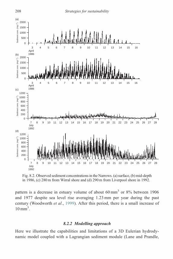
pattern is a decrease in estuary volume of about 60mm3 or 8% between 1906and 1977 despite sea level rise averaging 1.23mm per year during the pastcentury (Woodworth et al., 1999). After this period, there is a small increase of10mm3.

8.2.2 Modelling approach

Here we illustrate the capabilities and limitations of a 3D Eulerian hydrody-namic model coupled with a Lagrangian sediment module (Lane and Prandle,

(a)

(b)

(c)

(d)

Sed

imen

t con

c. (

mg

l–1)

Sed

imen

t con

c. (

mg

l–1)

Sed

imen

t con

c. (

mg

l–1)

Sed

imen

t con

c. (

mg

l–1)

2000

1500

1000

500

0

3April1986

April1986

July1992

July1992

4 5 6 7 8 9 10 11 12 13 14 15 16

3 4 5 6 7 8 9 10 11 12 13 14 15 16

7 8 9 10 11 12 13 14 15 16 17 18 19 20 21 22 23 24 25 26 27 28

7 8 9 10 11 12 13 14 15 16 17 18 19 20 21 22 23 24 25 26 27 28

2000

1500

1000

500

0

1200

1000

800

600

400

200

0

1200

1000

800

600

400

200

0

Fig. 8.2. Observed sediment concentrations in theNarrows. (a) surface, (b)mid-depthin 1986, (c) 280m from Wirral shore and (d) 290m from Liverpool shore in 1992.

208 Strategies for sustainability

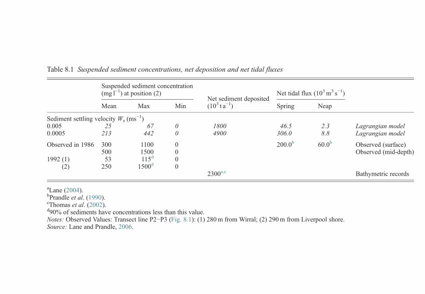
Table 8.1 Suspended sediment concentrations, net deposition and net tidal fluxes

Suspended sediment concentration(mg l−1) at position (2)

Net sediment depositedNet tidal flux (103m3 s−1)

Mean Max Min (103 t a−1) Spring Neap

Sediment settling velocity Ws (ms−1)0.005 25 67 0 1800 46.5 2.3 Lagrangian model0.0005 213 442 0 4900 306.0 8.8 Lagrangian model

Observed in 1986 300 1100 0 200.0b 60.0b Observed (surface)500 1500 0 Observed (mid-depth)

1992 (1) 53 115d 0(2) 250 1500d 0

2300a,c Bathymetric records

aLane (2004).bPrandle et al. (1990).cThomas et al. (2002).d90% of sediments have concentrations less than this value.Notes: Observed Values: Transect line P2−P3 (Fig. 8.1): (1) 280m from Wirral; (2) 290m from Liverpool shore.Source: Lane and Prandle, 2006.

2006) to quantify impacts on the estuarine sediment regime and indicate therate and nature of bathymetric evolution. Particular emphasis is on quantifyingthe variations in sediment concentrations and fluxes in sensitivity tests of bedroughness, eddy viscosity, sediment supply (particle sizes 10–100 μm), salinityintrusion and 2D versus 3D formulations of the hydrodynamic model. Themodel was not intended to reproduce bed-load transport associated with coarsersediments.Recognising the limited capabilities to monitor the often extremely heteroge-

neous SPM, a wide range of observational data were used for assessing modelperformance. These include suspended concentrations (axial profiles of mean and‘90th percentile’), tidal and residual fluxes at cross sections, estuary-wide netsuspension and deposition on spring and neap tides, surficial sediment distributionsand sequences of bathymetric evolution.The Eulerian hydrodynamic model provides velocities, elevations and diffusivity

coefficients for the Lagrangian ‘random-walk’ particle model in which up to amillion particles represent the sediment movements. It includes a wetting-and-dryingscheme to account for the extensive inter-tidal areas. Forcing involved specifyingtidal elevation constituents at the seaward limit in the Mersey Narrows, and riverflow at the head. The model uses a 120-m rectangular grid horizontally and a10-level sigma-coordinate scheme in the vertical.Calibration of the model (Lane, 2004) involved simulating effects of ‘perturba-

tions’, i.e. varying the msl, bed friction coefficients, vertical eddy viscosity and theriver flow. The optimum combination to minimise differences between observedandmodelled tidal elevation constituents was then determined. The model was mostsensitive to changes in bathymetries and bed friction coefficients, particularly in theinner basin. River flow only has an appreciable effect for discharges significantlyhigher than those usually encountered.

8.2.3 Lagrangian, random-walk particle modulefor non-cohesive sediment

Random-walk particle models replicate solutions of the Eulerian advection–diffusionequation by calculating, for successive time steps Δt, the height above the bed, Z,and horizontal location of each particle following

(1) a vertical advective movement – WS Δt (downwards),(2) a diffusive displacement l (up or down),(3) horizontal advection.

The displacement length l = √(2KzΔt) (Fischer et al., 1979), with the verticaleddy viscosity coefficient Kz approximated by fU*D, where f is the bed friction

210 Strategies for sustainability

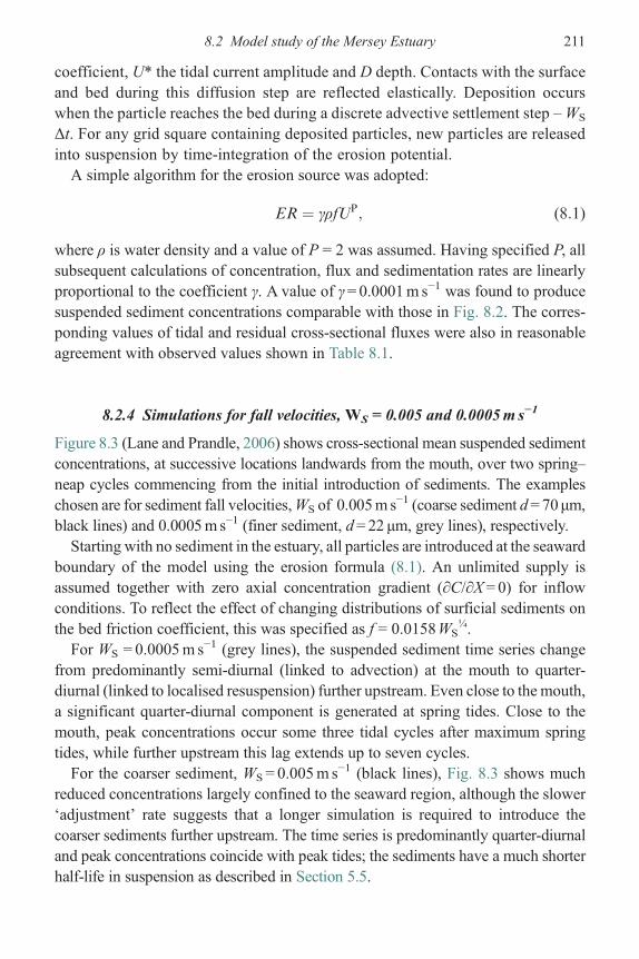
coefficient, U* the tidal current amplitude and D depth. Contacts with the surfaceand bed during this diffusion step are reflected elastically. Deposition occurswhen the particle reaches the bed during a discrete advective settlement step –WS

Δt. For any grid square containing deposited particles, new particles are releasedinto suspension by time-integration of the erosion potential.A simple algorithm for the erosion source was adopted:

ER ¼ γρfUP; (8:1)

where ρ is water density and a value of P = 2 was assumed. Having specified P, allsubsequent calculations of concentration, flux and sedimentation rates are linearlyproportional to the coefficient γ. A value of γ= 0.0001m s−1 was found to producesuspended sediment concentrations comparable with those in Fig. 8.2. The corres-ponding values of tidal and residual cross-sectional fluxes were also in reasonableagreement with observed values shown in Table 8.1.

8.2.4 Simulations for fall velocities, WS = 0.005 and 0.0005m s−1

Figure 8.3 (Lane and Prandle, 2006) shows cross-sectional mean suspended sedimentconcentrations, at successive locations landwards from the mouth, over two spring–neap cycles commencing from the initial introduction of sediments. The exampleschosen are for sediment fall velocities,WS of 0.005m s−1 (coarse sediment d=70μm,black lines) and 0.0005m s−1 (finer sediment, d=22μm, grey lines), respectively.Starting with no sediment in the estuary, all particles are introduced at the seaward

boundary of the model using the erosion formula (8.1). An unlimited supply isassumed together with zero axial concentration gradient (∂C/∂X= 0) for inflowconditions. To reflect the effect of changing distributions of surficial sediments onthe bed friction coefficient, this was specified as f = 0.0158WS

¼.For WS = 0.0005m s−1 (grey lines), the suspended sediment time series change

from predominantly semi-diurnal (linked to advection) at the mouth to quarter-diurnal (linked to localised resuspension) further upstream. Even close to the mouth,a significant quarter-diurnal component is generated at spring tides. Close to themouth, peak concentrations occur some three tidal cycles after maximum springtides, while further upstream this lag extends up to seven cycles.For the coarser sediment, WS = 0.005m s−1 (black lines), Fig. 8.3 shows much

reduced concentrations largely confined to the seaward region, although the slower‘adjustment’ rate suggests that a longer simulation is required to introduce thecoarser sediments further upstream. The time series is predominantly quarter-diurnaland peak concentrations coincide with peak tides; the sediments have a much shorterhalf-life in suspension as described in Section 5.5.

8.2 Model study of the Mersey Estuary 211

Figure 8.4(a) (Lane and Prandle, 2006) shows corresponding time series ofcumulative inflow and outflow of sediments across the mouth of the estuary model.Differences between inflow and outflow, in Fig. 8.4(b), indicate net suspension (highfrequency) and net deposition (low frequency). ForWS = 0.0005ms−1, the mean tidalexchange of sediments is around 110 000 t per tide, of which approximately 6% isretained amounting to 7000 t per tide. For WS = 0.005m s−1, the mean exchange is22 000 tonnes of which approximately 12% is retained or about 3000 t per tide.

Neap

1000

500

01000

500

01000

500

01000

500

01000

500

0500

0500

0500

500

500

500

500

0

0

0

0

00 2 4 6 8 10 12 14 16 18 20 22 24 26 28 30 32 34 36 38 40 42 44 46 48 50 52 54 56 58

Spring Neap

1

2

3

4

5

6

7

8

9

10

11

12

Semi-diurnal tidal cycles

Spring NeapNeap

Sus

pend

ed s

edim

ent c

once

ntra

tions

(m

g I–1

)

Fig. 8.3. Suspended sediment concentrations at 12 positions along the Mersey1 the mouth, 12 the head; grey lines settling velocityWS = 0.0005m s−1; black linesWS = 0.005m s−1.

212 Strategies for sustainability

8.2.5 Sensitivity to sediment size

Full details of the sensitivity tests are shown by Lane and Prandle (2006), these aresummarised in Tables 8.2 and 8.3. For a more extensive quantitative evaluation ofthe model, single neap–spring tidal cycle simulations were used. Results are sum-marised in Table 8.2 for particle diameters d from10 to 100μm.The model reveals that mean suspended sediment concentrations vary approxi-

mately with d −2. Equation (7.29a) indicates variability ranging from d0 to d−4 forfiner to coarser sediments. The extent of landward intrusion increases progressivelyfor finer sediments. A minimum capture rate of 2.8% occurs for d= 30 μm with

10(a)

(b)1.0

Net

dep

osite

d se

dim

ent (

mill

ion

tonn

es)

0.8

0.6

0.4

0.2

0

8

6

4

Cum

ulat

ive

sedi

men

t inf

low

/out

flow

(mill

ion

tonn

es)

2

00 2 4 6 8 10 12 14 16 18 20 22 24 26 28

Semi-diurnal tidal cycles

SpringNeap Neap

30 32 34 36

ws = 0.0005 m s–1

ws = 0.0005 m s–1

ws = 0.005 m s–1

ws = 0.005 m s–1

Inflow

Inflow

Outflow

outflow

Running-averageover tidal cycle

38 40 42 44 46 48 50 52 54 56 58

0 2 4 6 8 10 12 14 16 18 20 22 24 26 28Semi-diurnal tidal cycles

SpringNeap Neap

30 32 34 36 38 40 42 44 46 48 50 52 54 56 58

Fig. 8.4. Sediment fluxes at the mouth and net estuarine suspension and erosion.(a) Cumulative inflow and outflow at the mouth of the Mersey. (b) Net suspension(high frequency) and deposition (low frequency).

8.2 Model study of the Mersey Estuary 213

Table 8.2 Sensitivity of modelled sediments to particle diameters d from 10 to 100 μm for (a) maximum (90th percentile)concentrations; (b) mean concentrations; (c) estuarine-wide mean suspended and net deposited sediments on neap and springtides

(a)d(μm) 90th percentile suspended sediment concentrations (mg 1−1) at 2 km intervals upstream from the mouth

10 4186 3896 3804 3366 3274 3167 2471 1525 1052 714 560 470 500 348 309 217 16220 369 344 325 297 258 240 218 183 140 84 52 37 36 20 19 20 1230 169 148 133 101 89 67 47 29 12 6 3 2 2 – – – –40 140 118 103 75 64 45 26 12 5 3 2 1 1 – – – –50 108 95 83 62 53 35 16 7 4 3 2 1 1 – – – –60 83 72 65 47 39 22 8 3 1 – – – – – – – –70 63 56 50 38 29 16 5 1 – – – – – – – – –80 50 45 40 30 22 11 2 – – – – – – – – – –90 39 35 29 22 16 7 – – – – – – – – – – –

100 31 29 25 17 12 4 – – – – – – – – – – –

(b)d(μm) Mean suspended sediment concentrations (mg 1−1) at 2 km intervals upstream from the mouth

10 1645 1465 1423 1183 1118 1049 875 669 562 418 252 177 173 119 106 81 9220 176 157 151 128 120 108 93 75 60 43 27 17 15 8 7 5 530 68 56 47 34 27 20 14 8 4 2 1 – – – – – –40 51 41 33 22 17 11 6 3 1 1 – – – – – – –50 41 33 27 19 14 8 4 2 1 – – – – – – – –60 32 26 20 14 10 5 2 – – – – – – – – – –70 23 19 15 10 7 3 – – – – – – – – – – –80 18 14 11 7 5 2 – – – – – – – – – – –90 13 10 8 5 3 1 – – – – – – – – – – –100 10 8 6 3 2 – – – – – – – – – – – –

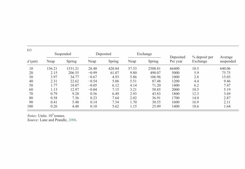
(c)Suspended Deposited Exchange

DepositedPer year

% deposit perExchange

Averagesuspendedd (μm) Neap Spring Neap Spring Neap Spring

10 156.21 1531.21 28.40 420.84 57.53 2508.81 66400 10.5 640.0620 2.15 206.55 −0.99 61.07 9.80 490.07 5000 5.9 75.7530 3.97 34.77 −0.67 4.93 5.86 106.96 1000 2.8 15.0340 2.31 22.62 −0.54 5.06 5.51 87.48 1200 4.4 9.4650 1.77 18.07 −0.05 6.12 4.14 71.20 1400 6.2 7.4760 1.13 12.97 −0.04 7.15 3.21 58.85 2000 10.5 5.1970 0.79 9.28 0.56 6.49 2.93 43.83 1800 12.3 3.6980 0.58 7.36 0.23 7.64 2.02 36.91 1700 14.0 2.8790 0.41 5.48 0.14 7.54 1.70 30.55 1600 16.9 2.11

100 0.26 4.48 0.10 5.62 1.15 25.09 1400 18.6 1.64

Notes: Units: 103 tonnes.Source: Lane and Prandle, 2006.

a corresponding deposition rate of 1Mt per year. While capture rates increaseprogressively with increasing sediment size (above d= 30 μm), correspondingdecreases in concentration yield a maximum deposition at 60 μm of 2Mt per year.This maximum is close to the preponderance of sediments with WS = 0.003m s−1

Table 8.3 Sensitivity of modelled sediments, R1–R8, forWS=0.0005m s −1 (d= 22μ)

(a)

RunMean suspended sediment concentrations (mg 1−1) at 2 km intervals upstream fromthe mouth

(1) 127 109 98 77 67 58 47 34 25 16 10 6 4 2 2 1 1(2) 333 304 301 263 253 234 205 171 141 106 71 50 49 35 29 23 25(3) 132 117 112 95 89 79 69 58 48 36 26 17 17 8 7 5 5(4) 127 112 104 84 76 69 56 43 32 21 12 7 5 2 2 1 1(5) 48 42 40 33 31 28 22 17 14 10 7 5 4 1 1 1 1(6) 196 171 155 127 116 105 86 60 42 24 12 7 5 2 1 1 1(7) 73 65 60 49 44 38 30 23 16 10 5 2 2 – 1 – –(8) 125 109 102 84 76 67 55 44 34 23 14 8 7 3 2 2 1

(b)

Run90th percentile suspended sediment concentrations (mg 1−1) at 2 km intervalsupstream from the mouth

(1) 290 250 229 182 166 144 118 86 63 40 24 16 16 10 9 7 9(2) 807 783 799 742 703 615 534 420 336 206 147 111 98 72 63 55 45(3) 279 259 257 218 208 186 171 148 114 81 63 48 52 31 24 22 18(4) 277 249 237 188 177 165 141 115 77 44 24 17 15 8 6 4 3(5) 90 84 82 70 67 62 53 44 37 28 18 16 16 8 6 7 5(6) 388 347 328 265 254 240 210 151 90 55 33 22 17 8 7 5 1(7) 149 137 133 107 99 93 81 59 36 18 11 8 7 4 4 1 1(8) 278 250 245 199 183 163 148 121 82 46 29 21 19 10 7 8 5

(c)Suspended Deposited Exchange

Depositedper year

% depositexchange

AveragesuspendedRun Neap Spring Neap Spring Neap Spring

(1) 8.58 70.21 −0.88 10.73 9.14 182.69 2200 3.8 31.03(2) 21.91 476.73 −1.20 118.22 11.49 1020.43 9300 5.9 167.55(3) 8.60 124.63 −1.17 30.70 8.41 289.48 3200 5.1 47.21(4) 7.78 121.18 −0.99 26.61 7.72 285.81 2700 4.3 45.21(5) 4.08 23.55 −0.58 2.83 4.44 60.80 800 3.5 11.84(6) 19.11 134.84 −1.51 23.94 17.92 310.08 3000 3.6 62.73(7) 6.62 61.39 −0.48 6.31 5.28 134.45 800 2.6 26.10(8) 8.32 116.75 −1.59 24.30 6.71 271.36 2500 4.2 44.54

Note: Units: 103 tonnesParameters as in Table 8.2.Diameter 22 μm, Ws = 0.0005m s−1.Source: Lane and Prandle, 2006.

216 Strategies for sustainability

(d= 54 μm) found by Hill et al. (2003). In Section 7.5, it was shown that the size ofsuspended sediments corresponding to ‘equilibrium’ conditions of zero net deposi-tion or erosion is in the range 20–50 µm. Throughout the range of d = 30–100 μm,net sedimentation remains surprisingly constant at between 1 and 2Mt per year.This sedimentation rate is in close agreement with observational evidence(Table 8.1).

8.2.6 Sensitivity to model parameters

Themodel’s responses to the following parameters were quantified: vertical structureof currents, eddy diffusivity, salinity, the bed friction coefficient and sediment supply.Table 8.3 shows, forWS = 0.0005m s−1 (d = 22 μm), the sensitivity to Run

numbers:

(R1) – No vertical current shear, i.e. a 2D hydrodynamic model.(R2) – Depth-varying eddy diffusivity , Kz(z) =Kz (−3z

2 + 2z+ 1), i.e. depth-mean value Kz

at the bed, 1.33Kz at z= Z/D = 0.33 and 0 at the surface(R3) – A time varying value of Kz(t), with a quarter-diurnal variation of amplitude 0.25Kz

producing a peak value 1 h after peak currents.(R4) – Mean salinity-driven residual current profile (4.15) Uz = gSxD

3/Kz (−0.1667z3 +

0.2687z2− 0.0373z− 0.0293), where the salinity gradient Sx was specified over a40 km axial length.

(R5) – Bed friction coefficient halved, f = 0.5 × 0.0158Ws¼.

(R6) – Bed friction coefficient doubled, f = 2.0 × 0.0158Ws¼.

(R7) – Erosion rate at the mouth 0.5 γ, i.e. halving the rate of supply of marine sediments.(R8) – Baseline simulation.

While the calculated values of sediment concentration and net fluxes varied widelyand irregularly, the net deposition remained much more constant. The acute andcomplex sensitivity to bed roughness and related levels of eddy diffusivity andviscosity is evident from Table 8.3. The acute sensitivity to bed roughnessand sediment supply leads to concern that migration of new flora and fauna mightlead to ‘modal shifts’ with potentially dramatic consequences.To comprehend these sensitivities, in shallow water we can approximate, from

Prandle (2004), the following dependencies on the friction factor f :

Tidal velocity amplitude U*� f −1/2

Sediment concentration C� f 1/2

Tidal sediment flux U*C� f 0

Residual sediment flux <UC>�U*C cos θ� f 1/2,

where θ is the phase lag of tidal elevation relative to currents and residual sedimentflux corresponds to net upstream deposition. These theoretical results are consistent

8.2 Model study of the Mersey Estuary 217

with the increases in concentration and residual fluxes for larger values of f shownby the model for both sediment types.

8.2.7 Summary

A century of bathymetric surveys indicate a net loss of estuarine volume of about0.1%, or 1 million cubic metres, per year. Similar percentage losses are found inmany of the large estuaries of NW Europe. Sea level rise of 1.2mma−1 representsonly a 0.02% annual increase. This relative stability persists in a highly dynamicregime with suspended sediment concentrations exceeding 2000mg 1−1 and springtide fluxes of order 200 000 t. Detailed analyses of the bathymetric sequencesindicate that most significant changes occur in the upper estuary and in inter-tidalzones. Long-period, up to 63 years, tidal elevation records in the lower estuary showalmost no changes to the predominant M2 and S2 constituents.A 3D Eulerian fine-resolution hydrodynamic model coupled with a Lagrangian,

random-walk sediment module was used to show how the dominant fluxes involvefine (silt) sediments on spring tides. The closest agreement between observed andmodel estimates of net imports of sediments occurs for sediments of diameter ofapproximately 50 μm – both dredging records and in situ observations indicatethat sediments of this kind predominate. The model showed little influence of riverflow, saline intrusion or channel deepening on the sediment regime. Conversely, thenet fluxes were sensitive to both the bed friction coefficient, f, and the phasedifference, θ, between elevation tidal velocity and elevation.Upper-bound rates of infill of up to 10Mt a−1 are indicated by the model,

comparable with annual dredging rates of up to 5Mt. The limited mobility ofcoarse sediments was contrasted with the near-continuously suspended nature ofthe finest clay. While the model indicated that sedimentation rates might increasesignificantly for much finer particles, this is likely to be restricted by the limitedavailability of such material in the adjacent coastal zone. The present approachcan be readily extended to study changes in biological mediation of bottomsediments, impacts of waves, consolidation and the interactions between mixedsediments.

8.3 Impacts of GCC

By 2050, GCC could significantly change mean sea levels, storminess, river flowsand, hence, sediment supply in estuaries (IPCC, 2001). The tidal and surge responsewithin any estuary will be further modified by accompanying natural morphological(post-Holocene) adjustments alongside impacts from past and present ‘interventions’.Generally, relatively small and gradual morphological adjustments are expected.

218 Strategies for sustainability

As an illustration, deposition per tide of a depth-mean concentration of 100mg l−1

in 10m water depth amounts to about 0.35mm, or 25 cm per year. In reality, asshown in the Mersey, ‘capture rates’ (upstream deposition as a proportion of thenet tidal inflow of suspended sediments) are typically only a few percent. Thus,simulations need to extend over decades to embrace responses over the full range offorcing cycles involved. However, as noted previously, longer-term extrapolationswith ‘Bottom-Up’ models become increasingly chaotic, and hence, here we exam-ine impacts from GCC by using the Theoretical Frameworks developed in earlierchapters.

8.3.1 Impacts on tide and surge heights

The response Framework, Fig. 2.5, based on analytical expressions derived byPrandle and Rahman (1980), provides immediate indications of likely changes inthe estuarine response of tides and surges. Figure 2.5 shows that amplification oftides (and surges) between the first ‘node’ and the head of the estuary can be up to afactor of 2.5. Concern focuses on conditions in estuaries where, for the excitation‘period’, P, the bathymetric dimensions (length, depth and shape) result in theestuarine mouth coinciding with this node with consequent resonant amplification.This occurs when, (2.26),

y ¼ 0:75 νþ 1:25; (8:2)

where y ¼ 4πL

Pð2�mÞðgDÞ1=2and v ¼ nþ 1

2�m:

L andD are the estuarine length and depth (at the mouth), andm is the power of axialdepth variation and n of breadth variation.The estuarine length, LR, for maximum amplification is then

LR ¼ ð2�mÞð0:75νþ 1:25Þ g1=2D1=2 P

ð4πÞ : (8:3)

The Framework extends from 0 < ν < 5 encompassing the following range ofshapes and associated resonant lengths:

ðaÞ canal m¼n¼ 0; ν ¼ 0:5 Lc ¼ 0:25ðgDÞ1=2PðbÞ embayment m¼n¼ 0:5; ν ¼ 1 L¼ 3=3:25Lc

ðcÞ linear m¼n¼ 1; ν ¼ 2 L¼ 2:75=3:25Lc

ðdÞ funnel m¼n¼ 1:5; ν ¼ 5 L¼ 2:5=3:25Lc:

(8:4)

Thus, as shown in Section 2.4.1, the range of funnelling (b) to (d) results in arelatively small reduction in the ‘quarter-wavelength’ resonant length applicable fora prismatic channel. Figure 8.5 indicates corresponding resonant periods for a

8.3 Impacts of GCC 219

semi-diurnal tidal period for a ‘linear’ estuary with m = n = 1. From (8.4), theseresults are broadly applicable for a wide range of estuarine shapes. The figureshows that even for a depth at the mouth of 4m, resonance at semi-diurnalfrequencies will only occur for LR > 60 km, while for D = 16m, LR > 100 km.From (8.3), for a synchronous estuary (m = n = 0.8, ν = 1.5), LR = 37 D1/2 (km) or94 km for the mean observed depth, D = 6.5m. This emphasises that onlythe longest of UK estuaries, such as the Bristol Channel, are likely to exhibitsignificant tidal amplification.Using the expression (6.12) for the length of a synchronous estuary

L ¼ 120D5=4

ðf&�Þ1=2(8:5)

with the bed friction coefficient f= 0.0025 and ς* tidal elevation amplitude. Byinserting (8.3) into (8.5), we derive the following expressions for resonant values ofLR and DR in terms of tidal amplitude, ς*:

LRðkmÞ � 180 &�1=3 (8:6)

and

DRðmÞ � 31&�2=3: (8:7)

Hence, for ς* = 1m, LR = 180 km and DR = 31m while for ς* = 4m, LR = 285 kmand DR = 78m.Thus, we only anticipate resonance at the semi-diurnal frequency in deep systems

such as the Bristol Channel where the estuarine ‘resonance’ extends to the adjacentshelf sea. Hence, we do not expect dramatic changes in tidal or surge responses in

12.5

25

50

100

2004 8

D (m)

L I (

km)

16 32 64

24

12

6

3

1.5

Fig. 8.5. Resonant periods (h) as a function of depth (at the mouth) and length.Results are for linear axial variations in depth and breadth, but from (8.4) are morewidely applicable.

220 Strategies for sustainability

estuaries for anticipated changes in sea level of up to 1m. Thus, increases in floodlevels due to rises in msl are likely to be of the same order as the respective increasesin adjacent open-sea conditions. Exceptions to the above are possible for surgeresponse to secondary depressions which can have effective periodicities of sig-nificantly less than 12 h and hence corresponding reductions in ‘resonant’ estuarinelengths.

8.3.2 Bathymetric adjustments

Chapter 6 shows how, for ‘synchronous’ estuaries, a ‘zone of estuarine bathymetry’can be determined bounded by

Ex

L51;

L1

L51 and

D

U3550m�2s3; (8:8)

corresponding to both tidal excursion, Ex, and salinity intrusion length, LI, beingless than estuarine length L and the Simpson–Hunter (1974) criterion, D/U3, for a‘mixed’ estuary.Figure 6.12 shows how Bar-Built and Coastal Plain estuaries in the UK generally

fit within this bathymetric zone. By introducing the expression (6.25) linking depthat the mouth to river flow and side slope gradient tan α

D0 ¼ 12:8ðQ tan αÞ0:4: (8:9)

Figures 7.9 and 7.10 show comparisons between observed lengths and depths (at themouth) against the theoretical values (8.5) and (8.9). The observed values wereextracted by Prandle et al. (2006) from the ‘FutureCoast’ database (Burgess et al.,2002).These Frameworks, Figs 6.12, 7.9 and 7.10, then provide immediate visual

indications of the likely stability and sensitivity of any particular estuary to changesinD,Q or ς*. Estuaries located within the bathymetric zone in Fig. 6.12, with depthsand lengths in broad agreement with the theoretical values in Figs 7.9 and 7.10,might be regarded as in present-day dynamic equilibrium. Consequently, futuremorphological adjustments might be expected to remain consistent with thesetheories and follow relatively rapidly. By contrast, estuaries outside the zone orwhere either depth or length is inconsistent with the theories might suggest anom-alous characteristics. By identifying the bases of such anomalies, the implicationsfor future morphology can be assessed.Clearly a sea level rise, of say 1m, will have a much bigger impact on shallow

estuaries than deep. Prandle (1989) examined the change in tidal response inestuaries due to variations in msl, where the locations of the coastal boundaries

8.3 Impacts of GCC 221

remained fixed (i.e. construction of flood protection walls). The results showed thelargest impacts in long, shallow estuaries.The theories synthesised in Figs 6.12, 7.9 and 7.10 do not consider sedimentation.

Changes in the nature and supply of marine sediments can lead to abrupt changes inestuarine morphology. This supply can directly determine the nature of the surficialsediments and thereby bed roughness. Changing flora and fauna can, via theireffects on sea-bed roughness and associated erosion and deposition rates, haveabrupt and substantial impacts on dynamics and bathymetry. Peculiarly, the relation-ship (8.9) between depth at the mouth and river flow is independent of both tidalamplitude and bed roughness. However, from (8.5), the associated estuarine lengthwill shorten as sediments become coarser.

8.3.3 Depth, breadth and length changes for 2100 variationsin msl and river flow

Estimates of ‘precautionary’ changes in msl by 2100 (Defra/Environment AgencyTechnical Summaries, 2003 and 2004) amount to an increase of 50 cm. Correspondingestimates for river fluxes include both increases and decreases of up to 25%.Inserting these changes in river flow, Q, into (8.9) and the resulting changes in

depth, δD, into (8.5), we can estimate the changes in length, δL. Likewise, thechanges in breadth, δB, associated with the changes in D can be estimated byassuming the side-slope gradients, tan α, are unchanged. Table 8.4 provides quanti-tative indications of the resultant changes. The representative values of D, L and Bover the range of estuarine geomorphologies were calculated from the FutureCoastdata set (Prandle, 2006).The changes δD correspond to δQ0.4, changes δL to (δQ0.4)1.25 and δB to 2δD/

tan α. The results show that, on average, the ‘dynamical’ adjustment to a 25%change in river flows may change depths by as much as the projected sea level

Table 8.4 Changes in depth, length and breadth for a 25% change in river flowand 0.5m increase in msl

Estuary type D (m) δDQ (±) L (km) δLQ (±) δLmsl (+) B (m) δBQ (±) δBmsl (+)

All minimum 2.5 0.25 5 0.62 1.28 130 38 77Mean 6.5 0.65 20 2.50 1.94 970 100 77All maximum 17.3 1.73 41 5.12 1.49 3800 266 77Coastal Plain 8.1 0.81 33 4.12 2.57 1500 147 91Bar-Built 3.6 0.36 9 1.12 1.59 510 51 71

Notes: Change in river flow – subscript ‘Q’, 0.5m increase in msl – subscript ‘msl’.Source: Prandle, 2006.

222 Strategies for sustainability

rise – with this effect reduced in smaller estuaries and significantly increased inlarger ones. The resulting changes in estuarine lengths and breadths follow similarpatterns with the bigger ‘dynamical’ changes occurring in the larger estuaries wherethey are significantly greater than those due to the specified sea level rise. Overall,we anticipate changes in estuarine lengths of the order of 0.5–5 km and breadths ofthe order 50–250m due to the 25% change in river flow. Corresponding changesdue a sea level rise of the order 50 cm involve increases in both lengths of order1–2.5 km and breadths of order 70–100m.

8.3.4 Impacts on currents, stratification, salinity,flushing and sediments

Indicative impacts of GCC on the above parameters can be similarly calculatedusing the respective parameter dependencies and Theoretical Frameworks sum-marised in Section 1.5. While the peculiar conditions in any specific estuary willdetermine the actual response, such immediate indications can provide usefulperspectives.

8.4 Strategies for modelling, observations and monitoring

8.4.1 Modelling

Coupled hydrodynamic and mixing models are required as the basis for transport-ing and mixing contaminants both horizontally and vertically. The dynamicalprocesses involved occur over time scales of seconds (turbulent motions), to hours(tidal oscillations), to months (seasonal variations) with corresponding space scalesfrom millimetres to kilometres. In addition to these hydrodynamic and mixingmodels, sediment and ecological models are required with robust algorithmsfor sources, sinks and biological/chemical reactive exchanges for longer-termsimulations.Both proprietary and public-domain model codes typically involve investment

of tens of years in software development and continued maintenance by sizeableteams. Such effort is increasingly beyond the resources of most modelling groups,and standardised, generic modules in readily available public-domain codes arelikely to be widely adopted. The development of such modules has removed muchof the mystique that traditionally surrounded modelling of marine processes. Thediversity of estuaries makes it unlikely that a single integrated model will evolve.Moreover, retention of flexibility at the module level is both necessary and desirableto accommodate a wide range of applications and to provide ensemble forecasts.Further developments of Theoretical Frameworks are important to interpret suchensemble simulations.

8.4 Strategies for modelling, observations and monitoring 223

To understand and quantify the full range of threats from GCC, whole-systemmodels are required – incorporating the impacts on marine biota and their potentialbiogeographic consequences. The introduction of various ‘Water FrameworkDirectives’ for governance of regional seas and coasts emphasises the need fordevelopment of well-validated, reliable models for simulating water quality, ecologyand, ultimately, fisheries. A systems approach is needed, capable of integratingmarinemodules and linking these into holistic simulators (geological, socio-economic, etc.).Rationalisation of modules to ensure consistency with the latter is an importantgoal, together with standardisation of prescribed inputs such as bathymetry andtidal boundary conditions. Such enhanced rationalisation will enable the essentialcharacteristics of various types of models to be elucidated including the inherentlimits to predictability.In practice, coupling might be limited to sub-set representations (statistical emu-

lators) encapsulating integrated parameters such as stratification levels or flushingtimes. To overcome the limitations of individual modules in such total-systemsimulations, methodologies are required both to quantify and to incorporate therange of uncertainties associated with model set-up, parameterisation and (futurescenario) forcing. This requirement can be achieved by ensemble simulations pro-viding relative probabilities of various outcomes linked to specific estimates of risk.Model simulations and assessments should extend beyond a single ebb and

flood cycle to include the spring–neap tidal cycle and seasonal variations in riverflows and related density structures. Clearer insights and understanding of scalingissues should emerge by comparing modelling results with the new TheoreticalFrameworks and against as wide a range of observational data as can be obtained.

8.4.2 Observations

Successful applications of models are generally limited by the paucity of resolutionin observational data (especially bathymetry) used for setting-up, initialising, for-cing (meteorological and along model boundaries), assimilation and validation.This paucity of data is a critical constraint in environmental applications. Moreand better observational data, extending over longer periods, are essential if model-ling accuracy and capabilities are to be enhanced.Instrumentation is lagging seriously behind model development and application,

and this gap is expected to widen. A new generation of instrumentation is needed forthe validation of species-resolving ecosystem models. Despite recent advances, therange of marine parameters that can be accurately measured is severely restrictedand the cost of observations is orders of magnitude greater than that associated withmodels.

224 Strategies for sustainability

Comprehensive observational networks are needed exploiting synergistic aspectsof the complete range of instruments and platforms and integrally linked to model-ling requirements. Permanent in situ monitoring is likely to be the most expensivecomponent of any observational network, and it is important to optimise suchnetworks in relation to the modelling system for the requisite forecasts.To define estuarine boundary conditions, there is a related requirement for

accurate (model) descriptions of the state of adjacent shelf seas. Permanent coastalmonitoring networks have been established in coastal seas and estuaries measuringwater levels, currents profiles, surface winds, waves, temperature, SPM, salinity,nutrients, etc. using tide gauges, mooring and drifting buoys, platforms, ferriesalongside remote sensing from satellites, radar and aircraft. Regional monitoringnetworks are being established via the Global Oceanographic Observing System(GOOS) networks, (UNESCO, 2003).Up-scaling of knowledge from small-scale experimental measurements is required

to provide larger- and longer-term algorithms employed in numerical models.Test-bed observational programmes are needed to assess model developments,these should ideally extend to water levels, currents, temperature and salinity,waves, turbulence, bed features, sedimentary, botanical, biological and chemicalconstituents. To maximise the value of such observations to the wider community,results should be made available in complete, consistent, documented and accessibleformats.

8.4.3 Monitoring

A basic monitoring strategy for studying bathymetric changes, capable of betterresolving processes operating in estuaries, should include the following:

(1) shore-based tide gauges throughout the length of an estuary, supplemented by waterlevel recorders in the deeper channels;

(2) regular bathymetric surveys, e.g. 10-year intervals with more frequent re-surveying inregions of the estuary where low water channels are mobile;

(3) a network of moored platforms with instruments for measuring currents, waves, sedi-ment concentrations, temperature and salinity.

Maximum use should be made of the synergy between satellite, aircraft, ship, seasurface, seabed and coastal (radar) instrumentation (Prandle and Flemming, 1998).Likewise, new assimilation techniques should be used for bridging gaps in monitor-ing capabilities. Observer systems sensitivity experiments can be used to determinethe value of the existence or omission of specific components in a new or existingmonitoring system.

8.4 Strategies for modelling, observations and monitoring 225

8.5 Summary of results and guidelines for application

Strategic planning to address long-term sustainability of estuaries needs to make fulluse of developments in modelling, monitoring and theory. New TheoreticalFrameworks provide a perspective on the threat from GCC.

The leading question is:How will estuaries adapt to GCC?

8.5.1 Challenges

Management challenges include

(1) promoting sustainable exploitation, i.e. permitting commercial and industrial developmentsubject to assessment of associated impacts, e.g. dredging, reclamation and fish-farming

(2) satisfying national and international legislation and protocols relating to discharges;(3) improving and promoting the marine environment, monitoring water quality, support-

ing diverse habitats and expanding recreational facilities;(4) reducing risks in relation to flooding, navigation and industrial accidents;(5) long-term strategic planning to address future trends including GCC.

A major difficulty in estuarine management is the general uncertainty in linkingspecific actions to subsequent responses over the local to wider scales and from theimmediate to longer time scales. For example, it has generally proved difficult topredict improvements to estuarine water quality following clean-up campaigns dueto leaching of contaminants from historical residues in bed sediments. Similarly, thefull impacts from ‘interventions’ may manifest themselves in unforeseen ways atremote sites at a much later time. While such uncertainties can never be entirelyovercome, the pragmatic objective is to arrive at a balanced perspective. Thisperspective should provide indications of the scale of vulnerability based on anensemble of ‘approaches’ using theory, measurements and modelling to draw onpresent and past behaviour of the estuary concerned and on related experiences inadjacent systems and in similar estuaries elsewhere.

8.5.2 Modelling case study

Section 8.2 describes a case study of a modelling simulation of the Mersey Estuary,indicating how theory and observational data are used to assess the model resultsand interpret parameter sensitivity tests. Figures 8.2 and Table 8.1 illustrate the useof results from earlier modelling and observational studies. Figures 8.3 and 8.4show results from a random-walk particle representation of sediment transport.This study highlights the value of long-term observational data sets. Unfortunately,

226 Strategies for sustainability

such data sets are overwhelmingly from large (navigable) estuaries and, as such, canbe misleading in relation to experience in smaller, shallower estuaries. Thus, inSection 8.3, the acute sensitivity of ‘near-resonant’ tidal responses in the Bayof Fundy (Garrett, 1972) and the Bristol Channel (Prandle, 1980) are shown tobe exceptional. Figure 8.5 indicates that resonant response for semi-diurnal tidalconstituents only occurs in estuaries greater than 60 km in length. The relateddemarcation between ‘inertially dominated’ systems and the much more commonlyencountered, shorter and shallower ‘frictionally dominated’ systems was shown inFig. 6.3.

8.5.3 Strategic planning

Section 8.4 considers future modelling and observational strategies. Strategicplanning for estuarine sustainability must encompass the wide spectra of tem-poral, spatial and parameter scales encompassing physics to ecology andmicro-turbulence to whole estuary circulation. Advantage must be taken of therapid advances in numerical modelling with the associated growth in computa-tional power, monitoring technologies and scientific understanding. However,securing investment in such advances generally requires demonstrable benefitsto end users.Faced with specific planning issues such as a proposed engineering ‘intervention’

or the need to improve flood protection, managers will often commission a model-ling study. The range of models available and their requirements was outlined inSection 1.4. It was indicated that the selection of an appropriate model depends onthe availability of observational data to set-up, initialise, force, validate and assesssimulations. Obtaining data is almost always much more expensive than a modelstudy.It is important to distinguish between model studies which involve ‘interpolation’

as opposed to ‘extrapolation’. The results illustrated in Tables 8.2–8.4 are essen-tially ‘interpolation’, i.e. examining small perturbations close to existing parameterranges. By contrast, ‘extrapolation’ involves larger perturbations which can changethe ranking of controlling processes and introduce new elements outside of therange of validity of the model.Ideally, an estuarine manager should have access to a range of modelling cap-

abilities, routinely assessed by a wide range of continuously monitored data.Confidence in future predictions then rests on the degree to which such modellingsystems can reproduce observed cycles, patterns and trends and interpret theseagainst Theoretical Frameworks. Development of a strategic programme needs toexploit all such technologies to provide the robust perspective required both forlong-term strategic planning and addressing specific day-to-day issues.

8.5 Summary of results and guidelines for application 227

8.5.4 Impacts of GCC

The success of new theories in explaining the evolution of morphologies over the past10000 years of Holocene adjustments lends confidence for their use in extrapolationover the next few decades. The explicit analytical formulae and Theoretical Frameworks,summarised in Section 1.5, can provide guidance on the relative sensitivity of an estuaryto both local ‘intervention’ and wider-scale impacts such as GCC. Figures 6.12, 7.9 and7.10 represent newmorphological frameworks. For any particular estuary, examining theloci on such frameworks frommouth to head and over the range of prevailing conditionscan provide a perspective on the relative stability. Where these loci extend outside of thetheoretical zones, the possibility of anomalous responses can be anticipated.We do not expect drastic changes in estuarine responses to tides or surges from

the projected impacts of GCC over the next few decades. Some enhanced sensitivitymight be found in relation to shorter ‘period’ (6 h) surges associated with secondarydepressions, particularly in larger estuaries. Maintaining fixed boundaries in theface of continuous increases in msl may enhance surge response in the shallowestestuaries (Prandle, 1989).In the absence of ‘hard geology’, enhanced river flowsmay result in small increases

in estuarine lengths and depths, developing over decades. By 2100, we anticipatechanges inUKestuaries due to (precautionary) projected 25%changes in river flow: oforder 0.5–5 km in lengths and of order 50–250m in breadths. Corresponding changesdue to a projected sea level rise of 50 cm are increases in lengths of order 1–2.5 km andbreadths of order 70–100m. In both cases, bigger changes will occur in largerestuaries. Althoughwe do not expect dramatic impacts on sediment regimes, changingflora and fauna could, through their effect on sea-bed roughness and associated erosionand deposition rates, have abrupt and substantial impacts on dynamics and bathymetry.Ultimately, an international approach is necessary to quantify the contribution to

and effect from GCC. This extends to development of models and instruments (andtheir platforms), planning of monitoring strategies, exchange of data, etc. The paceof progress will depend on successful collaboration in developing structuredresearch, development and evaluation programmes. The ultimate goal is a fusionof environmental data and knowledge, utilising fully the continuous development ofcommunications and computational capacities. Appendix 8A indicates technologieslikely to be widely available to estuarine managers in the next decade or so.

Appendix 8A

8A.1 Operational oceanography

Operational oceanography is defined as the activity of routinely making, dissemi-nating and interpreting measurements of coasts, seas, oceans and the atmosphereto provide forecasts, nowcasts and hindcasts.

228 Strategies for sustainability

8A.2 Forecasting, nowcasting, hindcasting and assimilation

Forecasting

Forecasting includes real-time numerical prediction of processes such as stormsurges, wave spectra and sea ice occurrence. Forecasts on a climatic or statisticalbasis may extend forward for hours days, months, years or even decades.Accumulation of errors, both from model inaccuracies and from uncertainties inforcing, limits realistic future extrapolations.

Nowcasting

In nowcasting, observations are assimilated in numerical models and the results areused to create the best estimates of fields at the present time, without forecasting.These observations may involve daily or monthly descriptions of sea ice, sea surfacetemperature, toxic algal blooms, state of stratification, depth of the mixed layer orwind–wave data.

Hindcasting

Observational data for hindcasting are assimilated into models to compile sets ofhistoric fields and distributions (typically monthly or annually) of variables such assea surface elevation, water temperature, salinity, nutrients, radio-nuclides, metalsand fish stock assessments.

Assimilation

Data assimilation forms the interface between models, observation and theory and,thus, is an essential component in simulation systems (Fig. 8A.1). Assimilationis used to transfer observed information to update the model state, the modelforcing and/or the model coefficients. The challenge is to take advantage of thecomplementary character of models and observations, i.e. the generic, dynamicallycontinuous character of process knowledge embedded in models alongside thespecific character of observed data.

Coupled models

ASSIMILATION

Set-up dataOperational

modelApplication End

user

AtmosphereOceanCoast

Monitoringnetwork

Bathymetry

SatelliteShipsBuoys, etc.

Initial conditions

Fig. 8A.1. Components of an operational modelling system.

Appendix 8A 229

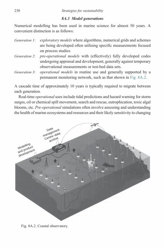
8A.3 Model generations

Numerical modelling has been used in marine science for almost 50 years. Aconvenient distinction is as follows:

Generation 1: exploratory models where algorithms, numerical grids and schemesare being developed often utilising specific measurements focusedon process studies.

Generation 2: pre-operational models with (effectively) fully developed codesundergoing appraisal and development, generally against temporaryobservational measurements or test-bed data sets.

Generation 3: operational models in routine use and generally supported by apermanent monitoring network, such as that shown in Fig. 8A.2.

A cascade time of approximately 10 years is typically required to migrate betweeneach generation.Real-time operational uses include tidal predictions and hazard warning for storm

surges, oil or chemical spill movement, search and rescue, eutrophication, toxic algalblooms, etc. Pre-operational simulations often involve assessing and understandingthe health of marine ecosystems and resources and their likely sensitivity to changing

Data

management

Centre–data

archive

Modelling

and product

development

Fig. 8A.2. Coastal observatory.

230 Strategies for sustainability

conditions. These are typically concerned with assessment of absorptive capacityfor licensing of discharges, evaluating environmental impacts of intervention (recla-mation, dredging, etc.) and climate change. Exploratory applications extend fromformulation of environmental management policies to developing the underpinningscience and technology to address both anthropogenic influences and natural trends.

8A.4 Forecasting

Even though the immediate issues of concern may seem far-removed from real-time‘operational’ forecasting, recognition of global-scale developments in modellingof marine systems is important. Ultimately, estuarine research needs to be linked tothe parallel progress in operational oceanography on both regional and global scalesdirected by GOOS (UNESCO, 2003). Effective operation of real-time forecastsrequires the resources of a meteorological agency for communications, processingand dissemination of forcing data, alongside oceanographic data centres responsiblefor dissemination of quality-controlled marine data.Amajor objective of operational oceanography is to minimise damage from future

events by reducing uncertainties in forecasting, ranging from storms on a shorttime scale to rising sea levels and temperatures over the longer term. Operationaloceanography is central to sustainable exploitation and management of our marineresources.Progress in aircraft and satellite remote sensing (Johannessen et al., 2000) will

dictate the rate of development of operational oceanography for many parameters.Lead times of a decade or more are required for development of new sensors,commercial production of prototype instruments and international agreement onnew satellite programmes. Remotely sensed data must be processed in hours if it isto be useful in operational forecasting. The need for enhanced information fromatmospheric models is a high-priority item in operational forecasting. As an exam-ple, accuracy and extent, in time ahead, of wind forecasts are the primary limitingfactors for wave and surge forecasting. The ultimate goal is dynamical coupling ofestuaries–seas–ocean marine models through to terrestial and atmospheric modules,i.e. global integration of water, thermal and chemical budgets (Prandle et al., 2005).

References

Burgess, K.A., Balson, P., Dyer, K.R., Orford, J., and Townend, I.H., 2002. FutureCoast –The integration of knowledge to assess future coastal evolution at a national scale. In:The 28th International Conference on Coastal Engineering. American Society of CivilEngineering, Vol. 3. Cardiff, UK, New York, pp. 3221–3233.

Defra/Environment Agency, 2003. Climate Change Scenarios UKCIP02: Implementationfor Flood and Coastal Defence. R&D Technical Summary W5B-029/TS.

References 231

Defra/Environment Agency, 2004. Impact of Climate Change on Flood Flows in RiverCatchments. Technical Summary W5-032/TS.

Fischer, H.B., List, E.J., Koh, R.C.Y., Imberger, J., and Brooks, N.H., 1979. Mixing inInland and Coastal Waters. Academic Press, New York.

Garrett, C., 1972. Tidal resonance in the Bay of Fundy. Nature, 238, 441–443.Hill, D.C., Jones, S.E., and Prandle, D., 2003. Dervivation of sediment resuspension rates

from acoustic backscatter time-series in tidal waters. Continental Shelf Research,23 (1), 19–40, doi:10.1016/S0278-4343(02) 00170-X.

Hutchinson, S.M. and Prandle, D., 1994. Siltation in the saltmarsh of the Dee Estuaryderived from 137Cs analysis of shallow cores. Estuarine, Coastal and Shelf Science,38 (5), 471–478.

IPCC, 2001. Edited by Watson, R.T. and Core Writing Team. Climate Change 2001:Synthesis Report. A Contribution of Working Groups I, II, and III to the ThirdAssessment Report of the Intergovernmental Panel on Climate Change. CambridgeUniversity Press, Cambridge, United Kingdom, and New York.

Johannessen, O.M., Sandven, S., Jenkins, A.D., Durand, D., Petterson, L.H., Espedal, H.,Evensen, G., and Hamre, T., 2000. Satellite earth observations in OperationalOceanography. Coastal Engineering, 41 (1–3), 125–154.

Lane, A., 2004. Bathymetric evolution of the Mersey Estuary, UK, 1906–1997: causes andeffects. Estuarine, Coastal and Shelf Science, 59 (2), 249–263.

Lane, A. and Prandle, D., 2006. Random-walk particle modelling for estimating bathymetricevolution of an estuary. Estuarine, Coastal and Shelf Science, 68 (1–2), 175–187,doi:10.1016/j.ecss.2006.01.016.

Pethick, J.S., 1984. An Introduction to Coastal Geomorphology. Arnold, London.Prandle, D., 1980. Modelling of tidal barrier schemes: an analysis of the open-boundary

problem by reference to AC circuit theory. Estuarine and Coastal Marine Science,11, 53–71.

Prandle, D., 1989. The Impact of Mean Sea Level Change on Estuarine Dynamics.C7-C14 in Hydraulics and the environment, Technical Section C: MaritimeHydraulics. Proceedings of the 23rd Congress of the IAHR, Ottawa, Canada.

Prandle, D., 2004. How tides and river flows determine estuarine bathymetries. Progress inOceanography, 61, 1–26, doi:10.1016/j.pocean.2004.03.001.

Prandle, D., 2006. Dynamical controls on estuarine bathymetries: assessment against UKdatabase. Estuarine, Coastal and Shelf Science, 68 (1–2), 282–288, doi:10.1016/j.ecss.2006.02.009.

Prandle, D. and Flemming, N.C. (eds.), 1998. The Science Base of EuroGOOS. EuroGOOS,Publication, No. 6. Southampton Oceanography Centre, Southampton.

Prandle, D. and Rahman, M., 1980. Tidal response in estuaries. Journal of PhysicalOceanography, 10 (10), 1522–1573.

Prandle, D., Lane, A., and Manning, A.J., 2006, New typologies for estuarine morphology.Geomorphology, 81 (3–4), 309–315.

Prandle, D., Los, H., Pohlmann, T., de Roeck Y-H., and Stipa, T., 2005. Modelling inCoastal and Shelf Seas – European Challenge. ESF Marine Board Postion Paper 7.European Science Foundation, Marine Board.

Prandle, D., Murray, A., and Johnson, R., 1990. Analyses of flux measurements in the RiverMersey. pp 413–430 In: Cheng, R.T. (ed.), Residual Currents and Long TermTransport, Coastal and Estuarine Studies, Vol. 38. Springer-Verlag, New York.

Price, W.A. and Kendrick, M.P., 1963. Field and model investigation into the reasons forsiltation in the Mersey Estuary. Proceedings of the Institute of Civil Engineers, 24,473–517.

232 Strategies for sustainability

Simpson, J.H. and Hunter, J.R., 1974. Fronts in the Irish Sea. Nature, 250, 404–406.Thomas, C.G., Spearman, J.R., and Turnbull, M.J., 2002. Historical morphological change

in the Mersey Estuary. Continental Shelf Research, 22 (11–13), 1775–1794,doi:10.1016/S0278-4343(02)00037-7.

UNESCO, 2003. The Integrated Strategic Design Plan for the Coastal Ocean ObservationModule of the Global Ocean Observation System. GOOS Report No. 125. IOCInformation Documents Series No. 1183.

Woodworth, P.L., Tsimplis, M.N., Flather, R.A., and Shennan, I., 1999. A review of thetrends observed in British Isles mean sea level data measured by tide gauges.Geophysical Journal International, 136 (3), 651–670.

References 233

Index

Annual Temperature Cycle 111–120global expressions air and sea surface

118–120heat-exchange components:

solar radiation 111, 112, 114, 117,latent heat flux 112infra-red back-radiation 112sensible heat flux 112

Analytical emulator 9, 10, 177–178, 184–187Asymmetry ebb-flood 40–44

Bathymetric: stability 10,Zone 16

Bathymetryexponential 35–38, 47power law 32–35, 47synchronous 27–31under-damped 36, 38over-damped 36, 38critical-damping 36, 38

Bed roughness 124–125Bessel Function 33

Circulation 2Climate Change 3, 12, 13, 16Coastal Observatory 16Convective overturning 84, 96–105,Coriolis 24Current componentsdensity-driven 52depth-mean 56maximum 57residual 69–70surface-bed changes 64–67tidal 53

amplitude 16related constituents 51structure 17

wind-driven 52, 67–69, 73Current ellipse 7, 59–62, 73–74a-c and c-w 61–62maximum amplitude 74minimum amplitude 74

direction 74phase 74eccentricity 74

Currents, sensitivity toeddy viscosity 62friction 62inter-tidal zone 67latitude 63–64tidal constituent 64

Decay time 2Declination 19Deposition/settlement rate 125, 144

boundary conditions: 130–131reflective bed 130, 143, 148absorptive bed 130, 148

delayed 143, 148exponential 132–134

Differential advection 83Dissipation

bottom friction 99vertical shear 99

Eddy diffusivity 97Eddy viscosity: 97

model 75–76formulation 57–59

Ekman Spiral 68, 73,Elliptic orbit 19Episodic events 2Equations of motion 24–25

1D momentum equation 1531D continuity equation 153

linearised friction term 153electrical-analogy 40,momentum 51, 53, 84steady state 90terms:

convective 42–43, 51–52Coriolis’ 72, 73density gradient 52inertial 42friction 43

234

non-linear 41–43surface-gradient 43

Equilibrium tide 20Erosion rate 125, 126–129

advective component 129in shallow water 128–129spring-neap cycle 127–128

Estuaries:age 11definition 1depth 16,length 16minimum depth and flow 168tidal dynamics 152–158

Estuary Response Diagram 33Estuary typologies: 196–199

bathymetry 196–198in-fill rates 199sediment regimes 198–199spacing between 169–170Theoretical Frameworks 205

Eulerian currents 70

Fall velocity 132Feed-back mechanism 11Flow Ratio 105–106Flushing time 2, 16, 97Friction 16, 47

linearization 38–39Froude Number 25

Gaussian distribution 130Global Climate Change 228

bathymetric adjustments 221–222changes to 222–223environmental effects 218impacts on tides and surges

219–221quarter-wavelength resonance 219

H F Radar 15, 68, 70Higher harmonics 3Hydraulic Scale Model 3

Inertia 16Inertial latitudes 53, 73,Internal waves 83

Kelvin Number 25

Lagrangian currents 70

Management Strategies 231modelling 223–224monitoring 225observations 224–225

Mean Sea Level 2, 11Mersey Estuary Study: 206–218

bathymetry 207–208hydrodynamic model 208–210Lagrangian sediment model 210–211

sediment regime: 206–207concentration & fluxes 211–212sensitivity to : particle size 213–217

model parameters 217–218tidal dynamics 206

Mixing 2classification:

Hansen-Rattray 79, 108Pritchard 79

effectiveness 104–105rates: 96–97

mixed salinity 96tidal straining 96river flow 96convective overturning : diffusivity 104

Models: 97–105forcing 15global 16resolution 13, 14, 15scope 13set-up 15validity 13development stage:

exploratory 230operational 228–231,pre-operational 230

modes of applicationassimilation 229forecasting 229, 231hindcasting 229nowcasting 229

types:Bottom-up 205Top-down 205

Monitoring : 16programme 12, 15sensors 15strategy 15, 16

Morphology 2

Net energy propagation 70Noise:Signal ratio 50

Observations 15Overturning 2

Peclet Number 129Potential Energy Anomaly 104Proxy data 4Phase difference(currents : elevation) 11

Process measurements 15

Q Factor 40Quarter wavelength resonance 26, 31, 34, 35

Residuals 3Remote sensing 15Richardson Number 80, 90, 106, 108Rouse Number 183Rotterdam Waterway 83

Index 235

Salinity intrusion 2, 16axial location 93–96, 160–161flushing times 159length 83, 90–96, 108, 158

derivations – experimental 90–91velocity components 91salt-wedge 92observations 93

residual current 86–88stratification 158

Schmidt Number 98Sea level gradient:river flow 85mixed-density gradient 86–87stratified density gradient 88wind-driven 89

Sediment characteristics 175–176concentration 16, 132delayed settlement 10, 176fall velocity 16flood-ebb dominance 177gravitational circulation 176half-life 11, 183suspended concentration 16, 132

analytical solution 131, 145–142sea-bed solution 131tidal spectra 135–137, 144–149vertical profile 134–135

trapping and sorting 10, 195–196sensitivity to:

coarse-fine 201–202half-life t50 194–195mouth-head 201–202neap-spring 201–202phase lag θ 194–195

turbidity maximum 176, 195–196vertical profile 183–184

Sediment fluxes: 186–190,equilibrium conditions 190–191erosion components 184–185export vs import : 178, 180–181, 193–195link to energetics 196suspension 185–186

sensitivity to: fall velocity 191–193bed friction 192–193

Sediment transport:modelling 124–125, 140–145observations 137–140

Seasonal cycles 2, 111–120Shear 2Spin-up time 24Stratification 16, 105–107, 110Number 106–107Simpson-Hunter 105–106Prandle 106

Stokes’ drift 70Strouhal Number 58–59, 62, 72,

73, 101Surface-to-bed differences:

velocity 99, 102–103, 107salinity 103–104

Sustainable exploitation 4Synchronous estuary: 9 14

bathymetric determinants 163–164definition 152Morphological Zone 161–163, 168observation vs theory 164–168shape 157–158solutions 27–31, 47, 154

current amplitude 29, 155depth profile 155estuarine length 155–156friction to inertia ratio 156saline intrusion 181–182sediment dynamics 182–184sensitivity to bed friction 29–30,

156–157tidal propagation 178, 180–181

Temperature 2, 111–120Test-bed data sets 15Theoretical Frameworks 17, 172–173Tides:

amphidrome 20constituents 19, 20,currents 14energy 2generation 17meso 1micro 1M2 constituent 2propagation 14straining 8, 83, 84, 96–105, 109

Tidal Responsediurnal 34higher-harmonics 40–44quarter-diurnal 34, 36semi-diurnal 33–34, 38, 46

Turbidity 2Turbidity Maximum 10, 195–196Turbulence 2, 14Turbulence model 64–67, 75–76

Vertical Structure:Salinity 89Currents 83, 101, 102–103

river flow 85–86mixed density gradient 86–87stratified density gradient 87–88wind-driven 89

236 Index