(This is a sample cover image for this issue. The actual ... greening, also called Huanglongbing...

(This is a sample cover image for this issue. The actual cover is not yet available at this time.)

This article appeared in a journal published by Elsevier. The attachedcopy is furnished to the author for internal non-commercial researchand education use, including for instruction at the authors institution

and sharing with colleagues.

Other uses, including reproduction and distribution, or selling orlicensing copies, or posting to personal, institutional or third party

websites are prohibited.

In most cases authors are permitted to post their version of thearticle (e.g. in Word or Tex form) to their personal website orinstitutional repository. Authors requiring further information

regarding Elsevier’s archiving and manuscript policies areencouraged to visit:

http://www.elsevier.com/copyright

http://www.elsevier.com/copyright

Author's personal copy

Spectral difference analysis and airborne imaging classification for citrusgreening infected trees

Xiuhua Li a,b, Won Suk Lee b,⇑, Minzan Li a, Reza Ehsani c, Ashish Ratn Mishra c, Chenghai Yang d, Robert L.Mangan d

a Key Laboratory of Modern Precision Agriculture Integration Research, MOE, China Agricultural University, Beijing 100083, Chinab Department of Agricultural & Biological Engineering, University of Florida, Gainesville, FL 32611, United Statesc Citrus Research and Education Center, University of Florida, 700 Experiment Station Road, Lake Alfred, FL 33850, United Statesd USDA-ARS, Kika de la Garza Subtropical Agricultural Research Center, Weslaco, TX 78596, United States

a r t i c l e i n f o

Article history:Received 4 September 2011Received in revised form 29 December 2011Accepted 16 January 2012

Keywords:Airborne imagingCitrus greeningDisease detectionImage classificationSpectral analysis

a b s t r a c t

Citrus greening, also called Huanglongbing (HLB), became a devastating disease spread through citrusgroves in Florida, since it was first found in 2005. Multispectral (MS) and hyperspectral (HS) airborneimages of citrus groves in Florida were acquired to detect citrus greening infected trees in 2007 and2010. Ground truthing including field and indoor spectral measurement, infection status along withGPS coordinates was conducted for both healthy and infected trees. Ground spectral measurementsshowed that healthy canopy had higher reflectance in the visible range, and lower reflectance in thenear-infrared (NIR) range than HLB infected canopy. Red edge position (REP) also showed notable differ-ence between healthy and HLB canopy. But the difference in the NIR range and REP were comparablymore sensitive to the environment or the background noise. Accuracy for separating HLB and healthysamples reached more than 90% when a simple REP threshold method was implemented in the groundreflectance datasets, regardless of field or indoor measurement; but it did not work well with the HSimages because of its low spatial resolution. Support vector machine (SVM) was able to provide a fast,easy and adoptable way to build a mask for tree canopy. High positioning error of the ground truth inthe 2007 HS image led to validation accuracy of less than 50% for most of classification methods. Inthe 2010 image from Southern Gardens (SG) grove, with better ground truth records, higher classificationaccuracies (about 90% in training sets, more than 60% in validation sets for most of the methods) wereachieved. Disease density maps were also generated from the classification results of each method; mostof them were able to identify the severely infected areas. Simpler classification methods such as mini-mum distance (MinDist) and Mahalanobis distance (MahaDist) showed more stable and balanced detec-tion accuracy between the training and validation sets in the 2010 images. Their similar infection trendwith ground scouted maps showed a promising future to manage HLB disease with airborne spectralimaging.

� 2012 Elsevier B.V. All rights reserved.

1. Introduction

1.1. Citrus Industry and HLB

As a major fruit crop in Florida, citrus produced about $1.47 bil-lion in 2009–2010, compared to $2.88 billion throughout the US,according to the citrus statistics by National Agricultural StatisticsServices (USDA, 2010). The whole citrus industry has about $9 bil-lion economic impact in Florida where nearly 569,000 acres of cit-rus groves exist.

However, this citrus industry is now greatly threatened by thecitrus greening disease (also known as Huanglongbing or HLB in

short). By February 2010, more than 3000 sections (one section isone square mile) were found infected by this disease in 34 countiesas shown in Fig. 1a (DPI, 2010). HLB infected trees have the initialappearance of asymmetric yellow patches on some of its leaves(Fig. 1b). As the bacteria spread within the tree, the entire canopyprogressively turns yellowish which may superficially resemblezinc deficiency. Fruit from severely infected trees are small, bitter,and often irregular in shape, which will totally destroy their eco-nomic value. The vector Diaphorina citri Kuwayama which origi-nated from Asia was discovered in June 1998 in Florida (Halbertand Manjunath, 2004), and the disease itself was first found inAugust 2005 in south Miami-Dade County, Florida (Manjunathet al., 2008).

The definitive diagnosis methods are mainly based on geneticmethodology such as polymerase chain reaction (PCR) (Jagoueix

0168-1699/$ - see front matter � 2012 Elsevier B.V. All rights reserved.doi:10.1016/j.compag.2012.01.010

⇑ Corresponding author.E-mail address: [email protected] (W.S. Lee).

Computers and Electronics in Agriculture 83 (2012) 32–46

Contents lists available at SciVerse ScienceDirect

Computers and Electronics in Agriculture

journal homepage: www.elsevier .com/locate /compag


et al., 1996). No effective and environmentally sound cure methodhas been found yet. The only preventative measure implementedtill now to slow down or reduce further infection is to removethe infected trees.

1.2. Citrus greening detection technologies

Although PCR test is so far the most accurate method to confirmHLB, samples should be first collected by trained workers, and thentested individually in a laboratory. The sampling and analysis pro-cess turns out to be highly labor intensive and time consuming,especially considering the wide grove area and the large numberof trees. So it is urgently required to find some other ways toquickly and accurately detect the infected trees.

Spectral reflectance (commonly measured in the visible andnear-infrared (NIR) spectral range) differs when the chemical com-ponents in the surface or subsurface of crop canopy change. Thiscausality provided researchers a nondestructive way to sense thechange happening inside the object. In agriculture, many studiesrelated to spectral features have been conducted to predict cropleaf chlorophyll content, nitrogen content, canopy diseases, etc.Pydipati (2004) and Qin et al. (2009) used color camera and hyper-spectral imaging system to differentiate some common symptom-atic citrus diseases by taking pictures of citrus’ leaves and fruitunder laboratory environment. Since one of the most obvioussymptoms of HLB is the change of canopy color to lighter greenand yellow, this imaging method could also be applied to detectHLB disease. Gonzalez-Mora et al. (2010) set up a ground basedprototype of hyperspectral sensing system which was designedto identify HLB infected trees, but the experimental result wasmuch affected by unrealistic illumination condition and unfavor-able timing. Fourier transform infrared–attenuated total reflection(FT-IR–ATR) spectroscopy was used by Hawkins et al. (2010) to testthe HLB disease in its earlier pre-symptomatic stages. As a substi-tute method of a PCR test, it took only minutes rather than hours totest a sample, and had a very high accuracy of 95%. However, forthis method, leaf samples needed to be collected, dried, and groundbefore analyzed.

Although the methods based on machine vision and spectrora-diometer mentioned above had a promising accuracy to distinguish

the diseased fruit or trees from healthy ones, it is still timeconsuming when applied to a large citrus grove due to their groundbased detection. Another extreme choice is satellite imagery whichhas a large field of view and has also been widely used in agricul-tural applications, such as vineyard leaf area estimation (Johnsonet al., 2003), sugarcane harvest detection (Hajj et al., 2009), etc.But it is difficult to conduct tree-based disease detection due toits coarse spatial resolution. This problem can be solved by adopt-ing airborne imaging which has a good balance of area coverageand image resolution compared to either ground measurementor satellite imagery.

Many studies on hyperspectral (HS) and multispectral (MS) im-age processing have been conducted in recent years, since satelliteand aircraft remote images are becoming easier to acquire. Noisereduction is one of the most important preprocessing steps, espe-cially for HS image which has large amount of correlated redun-dancy among its hundreds of different wavelength bands.Approaches such as principle component analysis (PCA), minimumnoise fraction (MNF), artificial neural network (ANN), etc. could beused for noise reduction or bands selection (Bajwa et al., 2004;Boardman and Kruse, 1994; Green et al., 1988).

Kumar et al. (2010) investigated several endmember detectionalgorithms to distinguish HLB infected citrus trees from healthyones based on MS and HS images, but more sufficient and convinc-ing ground spectral analysis is needed, and the classification accu-racy needs to be further improved. Huang et al. (2007) derivedphotochemical reflectance index (PRI) from both in-situ spectralreflectance measurement and airborne HS image to evaluate theyellow rust infection status in wheat, and the coefficients of deter-mination between PRI and infection severity reached to 0.97 and0.91 using in-situ spectral reflectance and airborne HS image,respectively.

Artificial neural network and support vector machines (SVMs)are also used in image pixel classification. In order to find outwhich method is more suitable for land use classification, Candadeand Dixon (2004) compared the application result with remote-sensing image classification by using these pattern recognitiontechniques.

In a study conducted by Plaza et al. (2009), good classificationperformance was demonstrated by SVMs using spectral signatures

Fig. 1. HLB infected sections and disease symptom: (a) HLB infected sections (marked in red) in Florida (DPI, 2010), and (b) HLB symptom on leaves and fruit. (Forinterpretation of the references to color in this figure legend, the reader is referred to the web version of this article.)

X. Li et al. / Computers and Electronics in Agriculture 83 (2012) 32–46 33


as input features, and was further improved by taking advantage ofsemi-supervised learning and contextual information. Several clas-sification algorithms for pattern recognition had also been tested inthe mapping of tropical forest cover using airborne HS data in a re-search conducted by Shafri et al. (2007). Results of maximum like-lihood, spectral angle mapping (SAM), artificial neural network(ANN), and decision tree classifiers were compared and evaluated.

Vegetation indices are also widely used for crop status evalua-tion or classification. Shafri and Hamdan (2009) used vegetationindices and red edge techniques derived from airborne hyperspec-tral image to detect ganoderma basal stem rot disease in oil palmplantations, and reported that red edge based techniques reachedthe highest accuracy of more than 80%. Qin and Zhang (2005) usedratio indices and stand difference indices from the four-band mul-tispectral airborne image to detect rice sheath blight disease, andreached a highest correlation coefficient of 0.68 with field diseaseindex. Tian et al. (2011) improved a technique to calculate red edgeposition (REP) for leaf nitrogen concentration (LNC) prediction inrice, and compared the accuracy with other techniques such as lin-ear extrapolation, Lagrangian technique, etc. by applying to aHyperion image, and reached higher coefficient of determinationwith leaf area index and leaf nitrogen concentration than othertechniques.

Although so many studies about remote sensing technologieshave been conducted, its application on HLB detection in citrusgroves was just started. In this study, advantages of both groundand airborne remote sensing were utilized to find the spectral dif-ferences between HLB and healthy citrus canopies. Several classifi-cation and spectral mapping methods were later implemented inairborne MS and HS images. Their performances and adaptabilityto detect HLB infected canopy in citrus groves were then comparedand evaluated.

2. Materials and methods

2.1. Image acquisition in 2007 and 2010

Airborne MS and HS images were acquired in 2007 and 2010, ata commercial citrus grove named Southern Garden (SG) in HendryCounty, FL, and a research grove in the Citrus Research and Educa-tion Center (CREC, affiliated to the University of Florida), LakeAlfred, FL.

The 2007 HS image was taken at northern part of the SG groveon November 3rd. The region of interest (ROI) spread across morethan 730 ha. The center coordinates were 26.385523�N,80.956000�W. Two orange varieties, Valencia and Hamlin, weregrown in this area. An AISA Eagle sensor was configured to collectthe HS data with 128 bands (ranging from 397 to 995 nm with aninterval of 4.7 nm). The raw data were radiometrically calibrated toradiance and then atmospherically corrected to reflectance by theFLAASH module in ENVI software (version 4.6, ITT VSI, WhitePlains, NY, USA). The final reflectance percentage values were mul-tiplied a factor of 100. The calibrated data were then georeferencedusing corresponding GPS and inertial measurement unit (IMU)information. The final mosaic image which was presented inUTM N17 projection with the datum of WGS-84 had a spatial res-olution of 0.7 m, and the estimated accuracy was approximately 1–2 pixels.

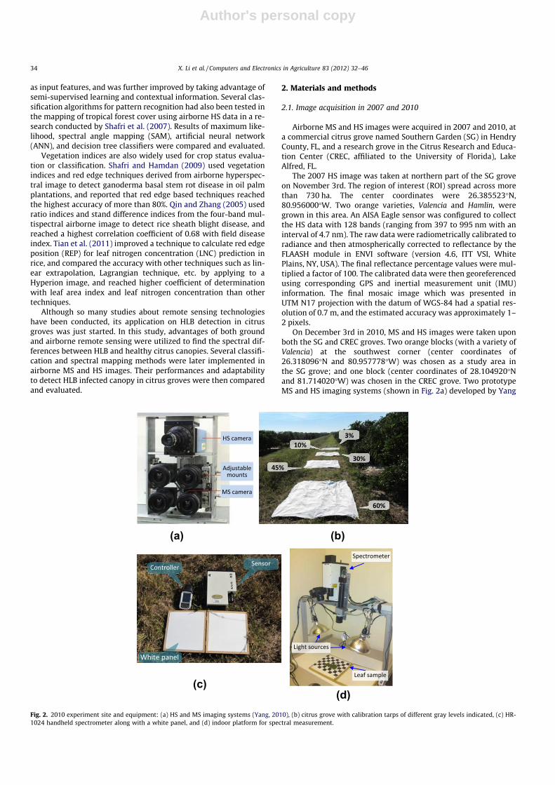
On December 3rd in 2010, MS and HS images were taken uponboth the SG and CREC groves. Two orange blocks (with a variety ofValencia) at the southwest corner (center coordinates of26.318096�N and 80.957778�W) was chosen as a study area inthe SG grove; and one block (center coordinates of 28.104920�Nand 81.714020�W) was chosen in the CREC grove. Two prototypeMS and HS imaging systems (shown in Fig. 2a) developed by Yang

(a) (b)

(c)(d)

Fig. 2. 2010 experiment site and equipment: (a) HS and MS imaging systems (Yang, 2010), (b) citrus grove with calibration tarps of different gray levels indicated, (c) HR-1024 handheld spectrometer along with a white panel, and (d) indoor platform for spectral measurement.

34 X. Li et al. / Computers and Electronics in Agriculture 83 (2012) 32–46


et al. (2003) and Yang (2010) were used in this experiment. The MSsystem consisted of four high resolution CCD cameras with fourband-pass filters at the wavebands of blue (430–470 nm), green(530–570 nm), red (630–670 nm), and NIR (810–850 nm). The HSimaging system integrated a CCD camera and an imaging spectro-graph which dispersed radiation into 128 bands in the range of457.2–921.7 nm (with an interval of 3.6 nm), and scanned in thealong-track direction. Alignment for the MS images and geometriccorrection for the HS images were conducted. For atmospheric cal-ibration, five 3 m � 3 m tarps with different gray levels (3%, 10%,30%, 45%, and 60%) were placed at an open area next to the citrusblocks while taking images, as shown in Fig. 2b. Their groundreflectance was also measured in both groves with a handheldspectrometer (HR-1024, Spectra Vista Corporation, Poughkeepsie,NY, USA, more detailed information found in Section 2.2)(Fig. 2c). By matching the ground reflectance of those tarps withtheir ROIs from images, empirical line was developed to radiomet-rically calibrate the raw digital number (DN) to reflectance. Withcorner coordinates collected with an RTK GPS equipment (HiPerXT, Topcon, Livermore, CA, USA), all the MS and HS images weregeoreferenced to UTM N17 projection with the datum of WGS-84. The MS images were resampled with 0.5 m resolution, andthe HS images were resampled with 1 m resolution. Basic informa-tion of these five images is listed in Table 1.

2.2. Ground truth measurement

In the 2007 experiment, the whole ROI was scouted by thegrove workers to check the infection status of each tree; howeverno PCR tests were performed to confirm the HLB infection. A totalof 7972 HLB infected trees along with their GPS coordinates wererecorded, however the positioning error was about 1–3 m. Noground spectral reflectance was measured. The 2007 experimentwas only used as a counterexample to prove the importanceof the ground truthing. In the 2010 experiment, four classes of

infection status were established based on symptom visibilityand PCR results at the SG grove; another five classes only basedon tree infection severity were established at the CREC grove.Table 2 lists the detailed information for all the classes.

Three types of ground truthing were investigated:

(a) Field and indoor spectral reflectance measurement for all theclasses.

(b) PCR tests to confirm HLB infected status of leaf samples.(c) Coordinates recording for all the measured trees by using an

RTK GPS receiver (HiPer XT, Topcon, Livermore, CA, USA)with a static horizontal accuracy of 3 mm.

Both field and indoor reflectance at the SG grove were measuredby the handheld spectrometer which was also used in the tarpmeasurement. It has a spectral range of 348–2505 nm with aninterval of 3 nm. A white reference panel made from polytetrafluo-roethylene (PTFE) material was used for calibration. The field mea-surement took advantage of solar radiation, and the indoormeasurement adopted an artificial light source.

The field measurement at the CREC grove was also carried outwith the same handheld spectrometer, but indoor measurementfor leaf samples, as well as branch and fruit samples was conductedwith another UV–VIS–NIR spectrophotometer (Cary 500 Scan, Var-ian, Palo Alto, CA, USA), which had better spectral resolution and anintegrating sphere for reflectance measurement. The spectral rangewas 200–2500 nm with a 1 nm interval.

2.3. Spectral feature analysis

Spectral features derived from original reflectance, such asabsorption and reflectance characteristics, first derivative (1D),red edge position, etc. from both ground measurement and air-borne images were analyzed and discussed.

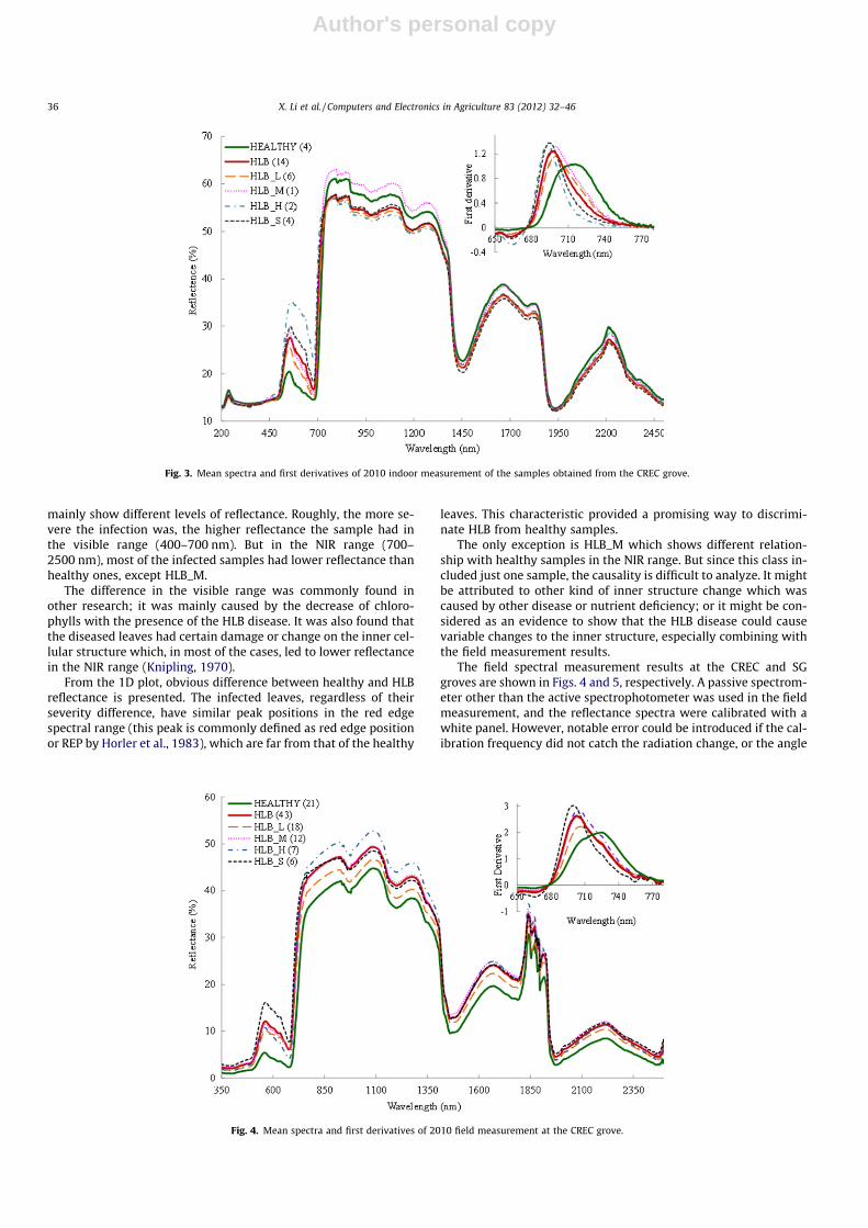
2.3.1. Spectral feature analysis from ground measurementMean spectra and 1D of every canopy class from the 2010 in-

door measurements in the CREC grove were calculated and areshown in Fig. 3. In the main plots, the dashed and dotted lines rep-resent classes with different HLB infection severity. The green andred solid lines represent the mean spectra for all the healthy andHLB infected samples, respectively. Those numbers in the paren-theses are the sample numbers for each class. The upper right sub-plot shows the 1D signature which was pre-processed with 11-stepmoving average for each class.

The indoor spectra shown in Fig. 3 were all about leaf samplesinstead of canopy. The spectrophotometer used in the indoorexperiment had its own light source, and every leaf sample wasplaced in an enclosed chamber, thus the result was very preciseand reliable. In Fig. 3, samples with different infection severity

Table 1Basic information for images used to detect HLB diseased canopy.

Images Spectral bands Spatialresolution (m)

2007 SG_HS 128-band HS image from 397 to 995 nm(4.7 nm interval)

0.7

2010 SG_HS 128-band HS image from 457.2 to921.7 nm (3.6 nm interval), acquired atthe Southern Gardens grove and CREC,respectively

1.02010 CREC_HS

2010 SG_MS 4-band MS image (at 450, 550, 650, and830 nm), acquired at the SouthernGardens grove and CREC, respectively

0.52010 CREC_MS

Table 2Brief description of four classes of leaf samples: only the class marked with ‘⁄’ was used to build a healthy library, and the class marked with ‘⁄⁄’ was used to build a HLB library.The other classes were not used in any library development. In the SG grove, ‘‘HEA’’ stands for ‘‘healthy’’, ‘‘S’’ stands for ‘‘symptom’’, ‘‘NS’’ stands for ‘‘non-symptom’’, ‘‘P’’ stands for‘‘positive’’, and ‘‘N’’ stands for ‘‘negative’’.

Imaging location Classes Tree infection status Infection status of sampled leaves

SG grove HEA_PCR_N� Healthy No HLB symptom, PCR tested negativeS_PCR_P�� HLB infected With HLB symptom, PCR tested positiveNS_PCR_N HLB infected No HLB symptom and PCR tested negativeNS_PCR_P HLB infected No HLB symptom but PCR tested positive

CREC grove HEALTHY Healthy No HLB symptom and PCR tested negativeHLB_L HLB infected Low HLB infection, PCR tested positiveHLB_M HLB infected Medium HLB infection, PCR tested positiveHLB_H HLB infected High HLB infection, PCR tested positiveHLB_S HLB infected Severe HLB infection, PCR tested positive



mainly show different levels of reflectance. Roughly, the more se-vere the infection was, the higher reflectance the sample had inthe visible range (400–700 nm). But in the NIR range (700–2500 nm), most of the infected samples had lower reflectance thanhealthy ones, except HLB_M.

The difference in the visible range was commonly found inother research; it was mainly caused by the decrease of chloro-phylls with the presence of the HLB disease. It was also found thatthe diseased leaves had certain damage or change on the inner cel-lular structure which, in most of the cases, led to lower reflectancein the NIR range (Knipling, 1970).

From the 1D plot, obvious difference between healthy and HLBreflectance is presented. The infected leaves, regardless of theirseverity difference, have similar peak positions in the red edgespectral range (this peak is commonly defined as red edge positionor REP by Horler et al., 1983), which are far from that of the healthy

leaves. This characteristic provided a promising way to discrimi-nate HLB from healthy samples.

The only exception is HLB_M which shows different relation-ship with healthy samples in the NIR range. But since this class in-cluded just one sample, the causality is difficult to analyze. It mightbe attributed to other kind of inner structure change which wascaused by other disease or nutrient deficiency; or it might be con-sidered as an evidence to show that the HLB disease could causevariable changes to the inner structure, especially combining withthe field measurement results.

The field spectral measurement results at the CREC and SGgroves are shown in Figs. 4 and 5, respectively. A passive spectrom-eter other than the active spectrophotometer was used in the fieldmeasurement, and the reflectance spectra were calibrated with awhite panel. However, notable error could be introduced if the cal-ibration frequency did not catch the radiation change, or the angle

Fig. 3. Mean spectra and first derivatives of 2010 indoor measurement of the samples obtained from the CREC grove.

Fig. 4. Mean spectra and first derivatives of 2010 field measurement at the CREC grove.



between solar incident light and object surface varied a lot. Onemore important difference from spectrophotometer measurementwas that even the spectrometer had a field of view (FOV) of only 4�,the targeting area still contained other background informationand radiation scattered from nearby objects. In the CREC experi-ment, calibration was conducted before every canopy measure-ment, and the white panel was kept at the same direction astargeted leaf surface. But in the SG experiment, calibration wasonly conducted once in a while.

In the CREC field result, the relationships between HLB andhealthy canopies in the visible and REP range are almost consistentwith the CREC indoor result, but quite different in the NIR range. Inthe SG field result, the REP difference was not as clear as in otherexperiments, showing that this indicator was also sensitive tobackground. The different relationship in the NIR range, on onehand, supported the conclusion that HLB disease can cause variablechanges in the NIR range; on the other hand, it also implied thatthe background had a qualitative influence on the reflectance inthe NIR range.

Since the samples were categorized by the symptom visibilityand PCR result in the SG experiment, the NS_PCR_P was consideredas being in the early stage of HLB disease because no visible symp-tom had been developed yet. Then another interesting point couldbe noticed in Fig. 5 that even though NS_PCR_P did not have anyvisible symptom, it still showed similar spectral reflectance withsymptomatic samples (S_PCR_P), suggesting a possibility to detectthe disease at early stage.

2.3.2. Spectral feature analysis from MS and HS imagesENVI (version 4.8, ITT VSI, White Plains, NY, USA) was used for

the MS and HS image analysis. First, pixels for different classes andland covers were collected to compare their spectral difference. Inthe 2007 hyperspectral image, due to the notable ground truthpositioning error, only infected trees rather than specific infectedcanopies could possibly be determined. In this case, four neighborpixels from the center of each infected tree were collected to buildan HLB infected library. Five other libraries for healthy tree canopy,grass, sand (bare ground in white color), soil (bare ground in siennacolor), and shadow were also manually collected from this image.Trees which were not marked in the ground truthing were consid-ered as healthy ones, and were randomly picked to build a healthy

canopy library. Grass was found between rows and at the edge ofevery block, and large area of shadow was formed at the east sideof every tree since the image was taken around 4 PM.

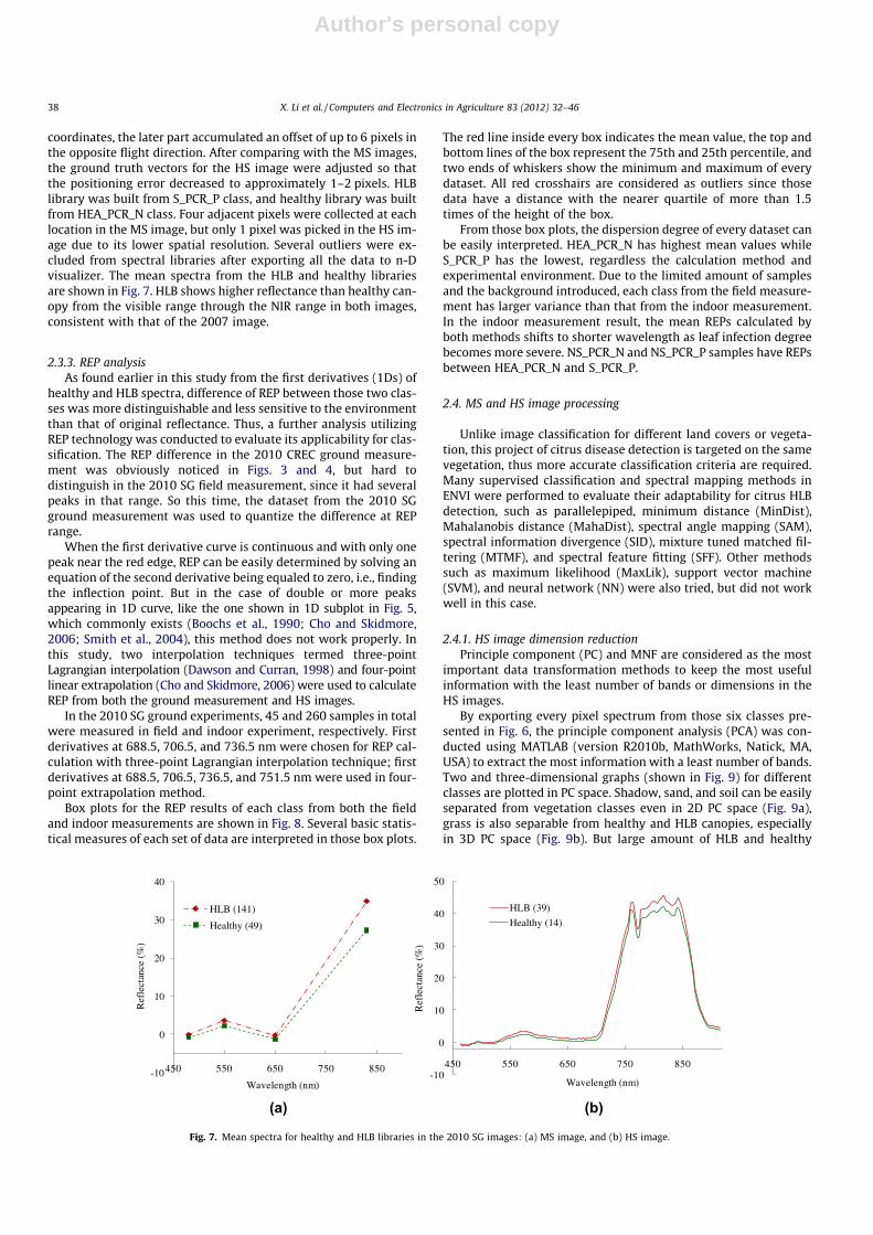
Mean spectra for those six libraries are plotted in Fig. 6. Num-bers in the parentheses in the legend area indicate the number ofpixels used for the mean calculation. This plot shows that sand,soil, shadow, and grass have obvious spectral difference than treecanopies, but HLB infected and healthy canopies have much lessdifference between them. The mean reflectance of HLB pixels isslightly higher than that of healthy ones in both the visible andNIR range. This trend is the same as the results of the 2010 CRECfield measurement.

In the 2010 images, more accurate ground truthing was imple-mented. However, the hyperspectral image from the CREC grovewas severely distorted that it was not suitable for classification,so only images from the SG grove were used for further analysis.The HS image from the SG grove, though, which was acquired bya pushbroom HS imaging prototype, still had an along-track distor-tion due to the decreasing flight speed. As a result, the later part ofthe original HS image had slightly higher spatial resolution thanthe previous one. After being georeferenced with corner

0

10

20

30

40

50

60

350 600 850 1100 1350 1600 1850 2100 2350

Ref

lect

ance

(%)

Wavelength (nm)

NS_PCR_P (10) NS_PCR_N (6)S_PCR_P (15) HEA_PCR_N (10)PCR_P (25) PCR_N (16)

3

6

9

12

15

400 500 600 700

Ref

lect

ance

(%)

Wavelength (nm)

-1

0

1

2

3

670 695 720 745

Fir

st d

eriv

ativ

e

Wavelength (nm)

Fig. 5. Mean spectra and first derivatives of 2010 field measurement at the SG grove.

0

20

40

60

80

100

120

400 500 600 700 800 900 1000

Ref

eclta

nce

(%)

Wavelength (nm)

Healthy (154)HLB (180)Grass (212)Shadow (319)Sand (191)Soil (99)

Fig. 6. Mean spectra of each class in the 2007 HS image.



coordinates, the later part accumulated an offset of up to 6 pixels inthe opposite flight direction. After comparing with the MS images,the ground truth vectors for the HS image were adjusted so thatthe positioning error decreased to approximately 1–2 pixels. HLBlibrary was built from S_PCR_P class, and healthy library was builtfrom HEA_PCR_N class. Four adjacent pixels were collected at eachlocation in the MS image, but only 1 pixel was picked in the HS im-age due to its lower spatial resolution. Several outliers were ex-cluded from spectral libraries after exporting all the data to n-Dvisualizer. The mean spectra from the HLB and healthy librariesare shown in Fig. 7. HLB shows higher reflectance than healthy can-opy from the visible range through the NIR range in both images,consistent with that of the 2007 image.

2.3.3. REP analysisAs found earlier in this study from the first derivatives (1Ds) of

healthy and HLB spectra, difference of REP between those two clas-ses was more distinguishable and less sensitive to the environmentthan that of original reflectance. Thus, a further analysis utilizingREP technology was conducted to evaluate its applicability for clas-sification. The REP difference in the 2010 CREC ground measure-ment was obviously noticed in Figs. 3 and 4, but hard todistinguish in the 2010 SG field measurement, since it had severalpeaks in that range. So this time, the dataset from the 2010 SGground measurement was used to quantize the difference at REPrange.

When the first derivative curve is continuous and with only onepeak near the red edge, REP can be easily determined by solving anequation of the second derivative being equaled to zero, i.e., findingthe inflection point. But in the case of double or more peaksappearing in 1D curve, like the one shown in 1D subplot in Fig. 5,which commonly exists (Boochs et al., 1990; Cho and Skidmore,2006; Smith et al., 2004), this method does not work properly. Inthis study, two interpolation techniques termed three-pointLagrangian interpolation (Dawson and Curran, 1998) and four-pointlinear extrapolation (Cho and Skidmore, 2006) were used to calculateREP from both the ground measurement and HS images.

In the 2010 SG ground experiments, 45 and 260 samples in totalwere measured in field and indoor experiment, respectively. Firstderivatives at 688.5, 706.5, and 736.5 nm were chosen for REP cal-culation with three-point Lagrangian interpolation technique; firstderivatives at 688.5, 706.5, 736.5, and 751.5 nm were used in four-point extrapolation method.

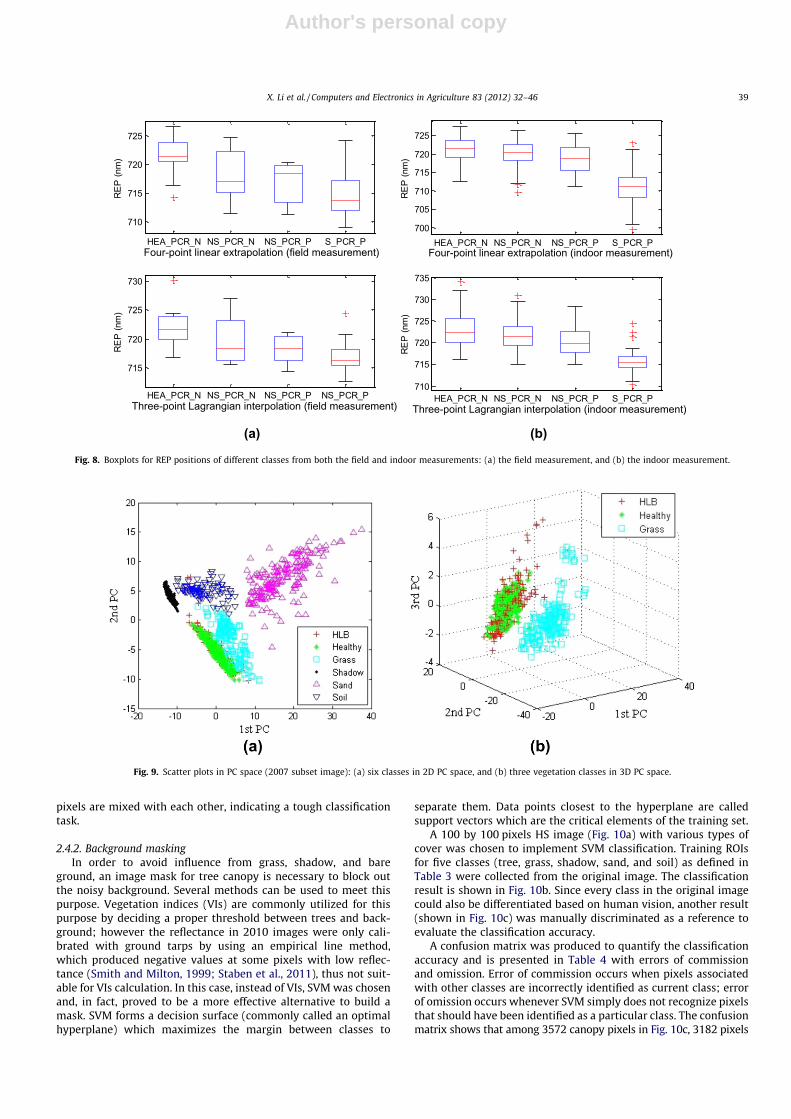
Box plots for the REP results of each class from both the fieldand indoor measurements are shown in Fig. 8. Several basic statis-tical measures of each set of data are interpreted in those box plots.

The red line inside every box indicates the mean value, the top andbottom lines of the box represent the 75th and 25th percentile, andtwo ends of whiskers show the minimum and maximum of everydataset. All red crosshairs are considered as outliers since thosedata have a distance with the nearer quartile of more than 1.5times of the height of the box.

From those box plots, the dispersion degree of every dataset canbe easily interpreted. HEA_PCR_N has highest mean values whileS_PCR_P has the lowest, regardless the calculation method andexperimental environment. Due to the limited amount of samplesand the background introduced, each class from the field measure-ment has larger variance than that from the indoor measurement.In the indoor measurement result, the mean REPs calculated byboth methods shifts to shorter wavelength as leaf infection degreebecomes more severe. NS_PCR_N and NS_PCR_P samples have REPsbetween HEA_PCR_N and S_PCR_P.

2.4. MS and HS image processing

Unlike image classification for different land covers or vegeta-tion, this project of citrus disease detection is targeted on the samevegetation, thus more accurate classification criteria are required.Many supervised classification and spectral mapping methods inENVI were performed to evaluate their adaptability for citrus HLBdetection, such as parallelepiped, minimum distance (MinDist),Mahalanobis distance (MahaDist), spectral angle mapping (SAM),spectral information divergence (SID), mixture tuned matched fil-tering (MTMF), and spectral feature fitting (SFF). Other methodssuch as maximum likelihood (MaxLik), support vector machine(SVM), and neural network (NN) were also tried, but did not workwell in this case.

2.4.1. HS image dimension reductionPrinciple component (PC) and MNF are considered as the most

important data transformation methods to keep the most usefulinformation with the least number of bands or dimensions in theHS images.

By exporting every pixel spectrum from those six classes pre-sented in Fig. 6, the principle component analysis (PCA) was con-ducted using MATLAB (version R2010b, MathWorks, Natick, MA,USA) to extract the most information with a least number of bands.Two and three-dimensional graphs (shown in Fig. 9) for differentclasses are plotted in PC space. Shadow, sand, and soil can be easilyseparated from vegetation classes even in 2D PC space (Fig. 9a),grass is also separable from healthy and HLB canopies, especiallyin 3D PC space (Fig. 9b). But large amount of HLB and healthy

(a) (b)

-10

0

10

20

30

40

450 550 650 750 850

Ref

lect

ance

(%

)

Wavelength (nm)

HLB (141)

Healthy (49)

-10

0

10

20

30

40

50

450 550 650 750 850

Ref

lect

ance

(%

)

Wavelength (nm)

HLB (39)

Healthy (14)

Fig. 7. Mean spectra for healthy and HLB libraries in the 2010 SG images: (a) MS image, and (b) HS image.



pixels are mixed with each other, indicating a tough classificationtask.

2.4.2. Background maskingIn order to avoid influence from grass, shadow, and bare

ground, an image mask for tree canopy is necessary to block outthe noisy background. Several methods can be used to meet thispurpose. Vegetation indices (VIs) are commonly utilized for thispurpose by deciding a proper threshold between trees and back-ground; however the reflectance in 2010 images were only cali-brated with ground tarps by using an empirical line method,which produced negative values at some pixels with low reflec-tance (Smith and Milton, 1999; Staben et al., 2011), thus not suit-able for VIs calculation. In this case, instead of VIs, SVM was chosenand, in fact, proved to be a more effective alternative to build amask. SVM forms a decision surface (commonly called an optimalhyperplane) which maximizes the margin between classes to

separate them. Data points closest to the hyperplane are calledsupport vectors which are the critical elements of the training set.

A 100 by 100 pixels HS image (Fig. 10a) with various types ofcover was chosen to implement SVM classification. Training ROIsfor five classes (tree, grass, shadow, sand, and soil) as defined inTable 3 were collected from the original image. The classificationresult is shown in Fig. 10b. Since every class in the original imagecould also be differentiated based on human vision, another result(shown in Fig. 10c) was manually discriminated as a reference toevaluate the classification accuracy.

A confusion matrix was produced to quantify the classificationaccuracy and is presented in Table 4 with errors of commissionand omission. Error of commission occurs when pixels associatedwith other classes are incorrectly identified as current class; errorof omission occurs whenever SVM simply does not recognize pixelsthat should have been identified as a particular class. The confusionmatrix shows that among 3572 canopy pixels in Fig. 10c, 3182 pixels

(a) (b)

HEA_PCR_N NS_PCR_N NS_PCR_P S_PCR_P

710

715

720

725

Four-point linear extrapolation (field measurement)

RE

P (n

m)

HEA_PCR_N NS_PCR_N NS_PCR_P NS_PCR_P

715

720

725

730

Three-point Lagrangian interpolation (field measurement)

RE

P (n

m)

HEA_PCR_N NS_PCR_N NS_PCR_P S_PCR_P700

705

710

715

720

725

Four-point linear extrapolation (indoor measurement)

RE

P (n

m)

HEA_PCR_N NS_PCR_N NS_PCR_P S_PCR_P710

715

720

725

730

735

Three-point Lagrangian interpolation (indoor measurement)R

EP

(nm

)

Fig. 8. Boxplots for REP positions of different classes from both the field and indoor measurements: (a) the field measurement, and (b) the indoor measurement.

Fig. 9. Scatter plots in PC space (2007 subset image): (a) six classes in 2D PC space, and (b) three vegetation classes in 3D PC space.



were classified correctly as tree canopy; 314, 75, and 1 pixelswere incorrectly classified as shadow, grass, and soil, respectively.The error of omission for tree class was 10.9%. However, most ofmisclassification happened between tree and shadow, which isobviously caused by the unclear boundary between those two clas-ses. Since this study was only concentrated on the bright canopyarea, this ambiguous area actually did not affect much on the finalresult. By ignoring this uncertain area, a modified error of omissionand commission for tree class can be re-calculated by Eq. (1) and(2), which were highly improved. The classification result for treecanopy was then used to build a mask for further HLB detection.

Modified error of omission for tree class :75þ 13572

� 100%

¼ 2:1% ð1Þ

Modified error of commission for tree class :242þ 91þ 6

3890� 100% ¼ 8:7% ð2Þ

2.4.3. Image classificationThe 2010 CREC images were not chosen for classification analy-

sis due to an obvious uncorrectable distortion observed in the HSimage. In the 2007 HS image, five 100 by 100 pixels subset images

were randomly chosen to implement classification methods. Twoof them were used as a training set, and the remaining threeformed a validation set. Eighty-two and 94 HLB infected trees werefound in the training and validation sets, respectively; the rest ofthe trees were considered healthy. HLB and healthy pixels fromthe training set were collected as libraries. In the 2010 SG images,most of the ground truth was concentrated in a small area shownin Fig. 11a. This area had 200 by 200 pixels in MS image and 100 by100 pixels in HS image. The right half area (200 by 100 for MS im-age, 100 by 50 for HS image) was used as a training set, and the lefthalf as a validation set. Pixels from S_PCR_P (39 samples) in thetraining area were collected as an HLB library (marked with redcrosshairs in Fig. 11a), and pixels from HEA_PCR_N (14 samples)in the training area (marked with white crosshairs in Fig. 11a)formed a healthy library.

Different classification methods were carried out through bothtraining and validation sets by using the library built from thetraining area. The classification result which best fit the groundtruth in the training set was then used to compare with the groundtruth in the validation set to calculate detection accuracy. In the2010 SG image, both S_PCR_P and NS_PCR_P classes were consid-ered as HLB infected trees (41 in the training area and 42 in the val-idation area) when calculating the detection accuracy.

A visualized plot of HLB and healthy training pixels in MS bandspace is shown in Fig. 11b. An overlap can be spotted between HLBpixels (red crosshairs) and healthy pixels (green ‘x’ marks).

To develop a better algorithm for HLB detection, the followingmethods were compared and evaluated: parallelepiped, minimumdistance (MinDist), Mahalanobis distance (MahaDist), spectral an-gle mapping (SAM), spectral information divergence (SID), spectralfeature fitting (SFF), and mixture tuned matched filtering (MTMF).

Parallelepiped classification forms a simple decision boundarywhich is an n-dimensional box or parallelepiped in image dataspace to classify data. MinDist actually refers to minimum distanceto class means; it is another simple method which only calculatesthe Euclidean distance between each unknown pixel vector andthe mean vector of each class. Compared to MinDist, MahaDistclassification not only calculates the Euclidean distance betweenunknown pixel and the mean, but also has directional sensitivity.It takes into account how noteworthy this distance is by calculat-ing statistical information of each dataset, but yet fast (Richardsand Jia, 2006).

SAM is a physical-based spectral classification method that usesan n-dimensional angle to match pixels to reference spectra. It wasdeveloped by Boardman (Kruse et al., 1993) which determined thesimilarity between two spectra by calculating the angle and treat-

Fig. 10. SVM classification accuracy evaluation (2007 subset image): (a) original subset image, (b) SVM classification result, and (c) manually defined ROIs by human vision.

Table 3ROI colors in the classification images and theircorresponding classes.

ROI color Class

Green Tree canopyCyan GrassRed, black ShadowBlue SoilMagenta Sand

Table 4Confusion matrix for SVM classification result.

Class (pixel) Tree Grass Soil Sand Shadow Commission (%)

SVM_Tree 3182 242 91 6 369 18.2SVM_Grass 75 781 19 2 23 13.2SVM_Soil 1 62 484 42 41 23.2SVM_Sand 0 0 15 245 0 5.8SVM_Shadow 314 89 288 8 3631 16.1

Total 3572 1174 897 303 4064Omission (%) 10.9 33.5 46.0 19.1 10.7



ing them as vectors in a space with dimensionality equals to thenumber of bands in use (Richards and Jia, 2006). All the four clas-sification methods mentioned above (parallelepiped, MinDist,MahaDist, and SAM) need to input proper threshold parameters.

SID is a stochastic spectral information measuring method. Itconsiders a spectrum as a random variable and measures the diver-gence between spectra. Smaller divergence indicates higher simi-larity (Chang, 1999; Du et al., 2004). Qin et al. (2009) found ahigh accuracy of 96.2% to detect citrus canker from normal peelsand other conditions based on the hyperspectral images taken ina laboratory condition.

Continuum removal is a newly developed method which is usedto normalize the band depth of spectra so that the depth differenceof each class can be more obvious and comparable. It mainly workson spectral absorption range, in other words, the reflectance spec-tra must have a concave in the range of interest (Kokaly and Clark,1999). The absorption feature retrieved in this method was foundto have a significant correlation with leaf nitrogen content, vegeta-tion coverage, etc. (Huang et al., 2004; Wen et al., 2008). SFF clas-sification method is directly based on this technology. A scaleimage and root mean square (RMS) image are outputted for each

class. Higher scale value and lower RMS error indicate a bettermatch with the library.

MNF transform was performed on all the HS images beforeimplementing MTMF. Every MNF band has an eigenvalue, whichrapidly decreases with band number (shown as Fig. 12). The largerthe eigenvalue is, the more abundant the information is. The first20 MNF bands were chosen to carry out MTMF mapping methodsince they had more significant eigenvalues. MTMF conductsmatched filtering (MF) on image and additionally adds an infeasi-bility image to the results which could be used to reduce the falsepositives found by MF. Pixels with a high infeasibility are likely tobe MF false positives. Parker Williams and Hunt (2002) analyzedthe coverage of leafy spurge by using MTMF method, and a highdetermination coefficient of 0.79 was reached when comparingwith the ground truth.

3. Results and discussion

3.1. Ground spectral separation result by REP technologies

To separate HEA_PCR_N and S_PCR_P samples by using groundreflectance spectra (dataset interpreted in Fig. 6), a simple methodof REP threshold could reach fairly high accuracy. Table 5 showsthe overall separation result. The indoor dataset (about 95%)reached higher accuracy than outdoor dataset (about 90%), becauseindoor measurement had more ideal environment and larger num-ber of samples. Four-point linear extrapolation technique yieldedbetter performance than three-point Lagrangian interpolation.Fig. 13a shows the REP result by four-point linear extrapolationfrom the 2010 SG indoor measurement. This result shows thatREP technique is a promising classification method, at least forground measurement.

Same techniques were then applied to the 2010 SG HS image,from where, 52 HEA_PCR_N pixels and 109 S_PCR_P pixels werechosen to calculate their REP by Lagrangian interpolation and lin-ear extrapolation, respectively. But neither of those methods pro-duced good result as shown in Fig. 13b which contains the resultcalculated by linear extrapolation, and little difference could befound. This is probably caused by the low spatial resolution of

Fig. 11. Subset image for classification and n-D Visualizer for the HLB and healthy libraries (from 2010 SG MS image): (a) true color image of the subset area; red crosshairsinfer to HLB infected tree samples, white crosshairs infer to healthy tree samples; the right half for training and left half for validation; (b) n-D Visualizer for HLB (red plus)and healthy (green cross) canopy libraries; Axes 1–4 represent the blue (480 nm), green (550 nm), red (650 nm), and NIR (830 nm) band in the MS image, respectively. (Forinterpretation of the references to color in this figure legend, the reader is referred to the web version of this article.)

Fig. 12. Eigenvalues for each band after MNF transform (from 2010 SG HS subsetimage).



the image which blurred out the characteristic found in groundmeasurement.

3.2. Image classification result

Fig. 14a1 shows part of the result conducted with MinDistmethod from the 2010 HS image. The green areas indicate healthytree canopies, and the red rectangles are the HLB detection results.

T-hec-

rosshairs show the infected trees which were confirmed by PCRtest. Fig. 14b shows part of the classification result by MinDist fromthe 2010 MS image.

Ground measured reflectance for HLB and healthy canopieswere used as libraries in SID and SFF spectral mapping methods.Fig. 15a shows the mean spectral library of HLB and healthy classesfrom the ground truth. The classification result by SID from the2010 HS subset image is shown in Fig. 15b.

Fig. 16 shows the classification result by SFF method. A scatterplot is presented in Fig. 16a, in which, x-axis represents the valuesfrom the scale image and y-axis represents the values from the

Table 5Separation results between HEA_PCR_N and S_PCR_P classes by using simple REP thresholds, where ‘‘LI’’ means Lagrangian interpolation, ‘‘LE’’ means linear extrapolation.

Experiment REP method Threshold (nm) Accuracy

Number of samples Pct. (%)

2010 SG field measurement (total sample number: 24) Three-point LI 719.8 21 87.5Four-point LE 720.0 22 91.7

2010 SG indoor measurement (total sample number: 136) Three-point LI 718.2 129 94.5Four-point LE 716.5 130 95.6

690

700

710

720

730

740

0 20 40 60 80

RE

P (n

m)

Sample number

HEA_PCR_N (52)

S_PCR_P (84)

715

720

725

730

735

740

0 20 40 60 80 100

RE

P (n

m)

Sample number

HEA_PCR_N (52)

S_PCR_P (109)

(a) (b)

Fig. 13. REP calculation results in the 2010 SG experiment: (a) REP calculated by four-point linear extrapolation from the indoor measurement, (b) REP calculated by four-point linear extrapolation from the HS image.

Fig. 14. MinDist and MahaDist classification results: (a) MinDist result from the 2010 HS image, and (b) MahaDist result from the 2010 MS image (validation set).

1 For interpretation of color in Figs. 3, 8, 14, 16, and 18, the reader is referred to theweb version of this article.



RMS image. Higher scale and lower RMS value indicates a bettermatch to the library. The lower right corner in Fig. 16a was selectedas infected pixels which are also marked out (red rectangles) inFig. 16b.

As shown in Fig. 17, a similar scatter plot was generated whenMTMF was implemented. x-axis is the MF score, and y-axis is theinfeasibility. Every pixel was plotted in the scatter plot accordingto their MF scores and infeasibility values which were calculatedby MTMF mapping method. Pixels which had high MF scores andlow infeasibility values (mapping in the lower-right corner in the

scatter plot) were selected out as the infected pixels. Fig. 17bshows the corresponding pixels marked in Fig. 17a.

3.3. Classification result comparison

Since all the ground truth coordinates could only reach tree-le-vel positioning accuracy, average values of neighboring pixels wereadopted to build the HLB and healthy libraries, therefore, only tree-based accuracy rather than pixel-based accuracy could be calcu-lated in the classification results. Even though the whole SG grove

Training setValidation set-10

0

10

20

30

40

50

60

460 560 660 760 860

Wavelength (nm)

HLBHealthy

(a) (b)

Ref

lect

ance

(%)

Fig. 15. SID classification result from the 2010 HS image: (a) imported library from the ground measured reflectance, and (b) SID classification result.

Training setValidation set

0.1

0.2

0.3

0.4

0 0.2 0.4 0.6

RM

S (H

LB)

Scale (HLB)

(a) (b)

Fig. 16. SFF classification result from the 2010 HS image: (a) SFF scatter plot, and (b) SFF classification result.

0

4

8

12

16

20

-2 -1 0 1 2

Infe

asib

ility

(HLB

)

MF Score (HLB) Validation set Training set

(a) (b)

Fig. 17. MTMF mapping result from the 2010 HS image: (a) MTMF scatter plot, and (b) MTMF classification result.



were roughly scouted, and infected trees were recorded by grow-ers, but no PCR tests were conducted to ensure their infection sta-tus. Also the positioning errors were too notable to ignore. So itwas difficult to count the overall detection accuracy, and onlydetection accuracy about the PCR confirmed trees could be calcu-lated. Table 6 includes all the tree-based classification accuracy

for both training and validation sets in the images taken at theSG grove.

The classification results for the 2007 HS image are not good.The highest correct identification rates are 75.6% for the trainingset, and 53.2% for the validation set. The main reasons for theselow accuracies are: (a) HLB and healthy libraries built from theground truth in the 2007 experiment were not accurate due tothe high positioning error; (b) the 2007 HS image had five subsetimages from different areas, radiometric differences between eachsubset (may be caused by the geographic changes, atmosphericparticulate variation, etc.) also had negative influence on the clas-sification results.

The 2010 images yielded much better results than the 2007 im-age. SFF showed very good accuracy of 95.1% in the training set and90.2% in the validation set in the 2010 HS image, but it did notwork well in the MS image, implying that SFF was not a good ideafor this four-band MS image. More (but not too many) bands wouldbe needed for a better result. SID yielded abnormal result in the2010 MS image (detection accuracy in the validation set was muchhigher than that in the training set), which indicated unstable per-formance in this application. SAM performed very well in the train-ing set, but its accuracy decreased significantly in the validationset. Simpler classification methods like MinDist and MahaDistshowed more stable performance in the 2010 images, as theyhad more balanced accuracies between the training and the valida-tion sets.

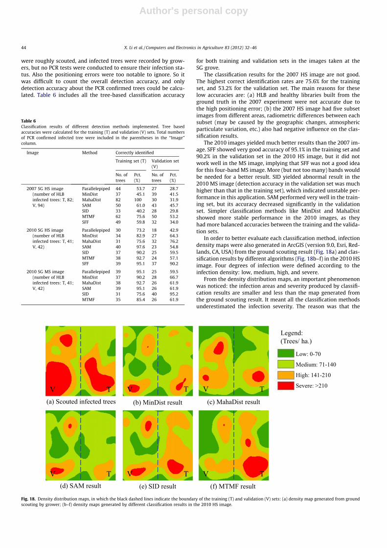
In order to better evaluate each classification method, infectiondensity maps were also generated in ArcGIS (version 9.0, Esri, Red-lands, CA, USA) from the ground scouting result (Fig. 18a) and clas-sification results by different algorithms (Fig. 18b–f) in the 2010 HSimage. Four degrees of infection were defined according to theinfection density: low, medium, high, and severe.

From the density distribution maps, an important phenomenonwas noticed: the infection areas and severity produced by classifi-cation results are smaller and less than the map generated fromthe ground scouting result. It meant all the classification methodsunderestimated the infection severity. The reason was that the

Table 6Classification results of different detection methods implemented. Tree basedaccuracies were calculated for the training (T) and validation (V) sets. Total numbersof PCR confirmed infected tree were included in the parentheses in the ‘‘Image’’column.

Image Method Correctly identified

Training set (T) Validation set(V)

No. oftrees

Pct.(%)

No. oftrees

Pct.(%)

2007 SG HS image(number of HLBinfected trees: T, 82;V, 94)

Parallelepiped 44 53.7 27 28.7MinDist 37 45.1 39 41.5MahaDist 82 100 30 31.9SAM 50 61.0 43 45.7SID 33 40.2 28 29.8MTMF 62 75.6 50 53.2SFF 49 59.8 32 34.0

2010 SG HS image(number of HLBinfected trees: T, 41;V, 42)

Parallelepiped 30 73.2 18 42.9MinDist 34 82.9 27 64.3MahaDist 31 75.6 32 76.2SAM 40 97.6 23 54.8SID 37 90.2 25 59.5MTMF 38 92.7 24 57.1SFF 39 95.1 37 90.2

2010 SG MS image(number of HLBinfected trees: T, 41;V, 42)

Parallelepiped 39 95.1 25 59.5MinDist 37 90.2 28 66.7MahaDist 38 92.7 26 61.9SAM 39 95.1 26 61.9SID 31 75.6 40 95.2MTMF 35 85.4 26 61.9

Legend:(Trees/ ha.)

(a) Scouted infected trees (b) MinDist result (c) MahaDist result

(d) SAM result (e) SID result (f) MTMF result

V T V T V T

V T V T V T

Low: 0-70

Medium: 71-140

High: 141-210

Severe: >210

Fig. 18. Density distribution maps, in which the black dashed lines indicate the boundary of the training (T) and validation (V) sets: (a) density map generated from groundscouting by grower; (b–f) density maps generated by different classification results in the 2010 HS image.



classification thresholds were only determined to maximallymatch the PCR confirmed ground truth which was not fully inves-tigated for all the trees. This problem can be solved by investigat-ing ground truth comprehensively in the training area.

Putting aside the difference of infection severity, MahaDistyielded the best match with the trend of the ground scouted truthmap. Since MinDist measures the Euclidean distance from librarymean, and SAM is essentially the Euclidean distance (Du et al.,2004) when the spectral angle is small (which is exactly the casein this study because this HLB disease detection is actually basedon the same kind of canopy), they produced very similar resultswith each other. SID and MTMF relatively overestimated the infec-tion situation in the training set and underestimated it in the val-idation set, indicating an over-fitting problem. But no matterwhich method was used, the most severely infected areas (redareas in Fig. 18a) were all pointed out, showing a great potentialto support citrus grove management. This also indicated that themore severe the disease is, the easier it can be identified. In oneword, airborne image could be used to assist citrus grove manage-ment since it was capable of detecting the HLB disease with obvi-ous symptom and infection area. Fast and semi-automaticdetection procedure could be developed as long as the groundtruth in the training area could be investigated as the input.Thresholds in the classification methods could be manuallydecided. More comprehensive and precise ground truth investiga-tion would produce higher accuracy.

From both the quantified accuracy results and the density maps,the relatively simpler methods – MinDist and MahaDist showedmore stable and balanced performance than the rest, thus theywere highly recommended in a future study.

Some problems were encountered during this research, espe-cially in the field experiments. To get better results, the followingimprovements or suggestions needed to be taken intoconsideration:

(1) Low classification accuracy and high false positive werehighly related with large positioning error of the groundtruth. More precise ground truthing must be conducted.For example, specific infected canopy locations and areasother than the center coordinates of infected trees shouldbe recorded to exactly pinpoint the research targets. Reliableimaging system was another critical concern to ensure highquality images.

(2) Except MTMF, all other classification or spectral mappingmethods were carried out in the original band space, how-ever other data spaces such as MNF space, PC space, etc.should be further considered for better classification results.

4. Conclusions

The MS and HS airborne images of citrus groves were acquiredto detect HLB infected trees. Ground truthing including groundreflectance measurement, tree infection status confirmation, andGPS coordinates recording was implemented to analyze the spec-tral features and build proper libraries for HLB infected and healthycanopies. The following are major findings:

(1) Spectral reflectance was analyzed. Ideally, the healthy can-opy had higher reflectance in the visible range, and lowerin the NIR range than the infected canopy. But the relation-ship in the NIR range was easily affected by measuring con-dition or environment.

(2) REP was comparably less sensitive to the environment thanthe reflectance in the NIR range. Separation accuracy of morethan 90% was reached when simple threshold method was

implemented within ground spectral datasets, regardless offield or indoor measurement; but still did not work wellwith HS images due to its low spatial resolution.

(3) SVM provided a fast, easy and adoptable way to build maskfor tree canopy to block out background pixels for furtherimaging classification.

(4) Several classification and spectral mapping methods wereconducted to evaluate their applicability for HLB detection.High positioning error of the ground truth in the 2007 HSimage led the validation accuracy to less than 50% for mostof the classification methods. However, with better groundtruthing data, the 2010 SG images reached higher accuraciesranging from 43% to 95%. Simpler classification methods,MinDist and MahaDist, showed more stable and balancedperformance between the training and validation sets, thusthose two methods were highly recommended in a futurestudy.

(5) Most of the methods were able to detect the severelyinfected areas in the density maps, and their similar infec-tion trend with that of scouted map could provide a promis-ing way to assist HLB disease management. Using theground truthing in the training area as the prior knowledge,procedures could be developed for rapid detection of theHLB disease.

Acknowledgements

The authors thank Ms. Ce Yang, Mr. Asish Skaria, Mr. FerhatKurtulmus, Mr. Anurag Katti, and Mr. John Simmons in the Preci-sion Agriculture Laboratory, Agricultural and Biological Engineer-ing Department, University of Florida for their kind support andassistance on the ground truthing experiment, statistical analysis,MATLAB programming, etc. This project was funded by the CitrusResearch and Development Foundation, Inc.

References

Bajwa, S.G., Bajcsy, P., Groves, P., Tian, L.F., 2004. Hyperspectral image data miningfor band selection in agricultural applications. Transactions of the ASAE 47 (3),895–907.

Boardman, J.W., Kruse, F.A., 1994. Automated spectral analysis: a geologic exampleusing AVIRIS data, north Grapevine Mountains, Nevada. Proceedings of theThematic Conference on Geologic Remote Sensing 10 (1), 407–418.

Boochs, F., Kupfer, G., Dockter, K., Kühbauch, W., 1990. Shape of the red edge asvitality indicator for plants. International Journal of Remote Sensing 11 (10),1741–1753.

Candade, N., Dixon, B., 2004. Multispectral classification of Landsat images: acomparison of support vector machine and neural network classifiers. In: ASPRSAnnual Conference Proceedings. Denver, Colorado.

Chang, C.I., 1999. Spectral information divergence for hyperspectral image analysis.Geoscience and Remote Sensing Symposium 1, 509–511.

Cho, M.A., Skidmore, A.K., 2006. A new technique for extracting the red edgeposition from hyperspectral data: the linear extrapolation method. RemoteSensing of Environment 101 (2), 181–193.

Dawson, T.P., Curran, P.J., 1998. A new technique for interpolating the reflectancered edge position. International Journal of Remote Sensing 19 (11), 2133–2139.

DPI, 2010. Section positive for Huanglongbing in Florida, HLB Bibliographicaldatabase, FDACS. Available from: <www.crec.ifas.ufl.edu/>.

Du, Y., Chang, C.I., Ren, H., Chang, C.C., Jensen, J.O., D’Amico, F.M., 2004. Newhyperspectral discrimination measure for spectral characterization. OpticalEngineering 43 (8), 1777–1786.

Gonzalez-Mora, J., Vallespi, C., Dima, C.S., Ehsani, R., 2010. HLB detection usinghyperspectral radiometry. In: 10th ICPA Proceedings. Available from: <http://www.andrew.cmu.edu/user/jlibby/robotany/Gonzalez-Mora-2010.pdf/>.

Green, A.A., Berman, M., Switzer, P., Craig, M.D., 1988. A transformation for orderingmultispectral data in terms of image quality with implications for noiseremoval. IEEE Transactions on Geoscience and Remote Sensing 26 (1), 65–74.

Hajj, M.E., Begue, A., Guillaume, S., Martine, J.F., 2009. Integrating SPOT-5 timeseries, crop growth modeling and expert knowledge for monitoring agriculturalpractices – the case of sugarcane harvest on Reunion Island. Remote Sensing ofEnvironment 113 (10), 2052–2061.

Halbert, S.E., Manjunath, K.L., 2004. Asian citrus psyllids (Sternorrhyncha, Psyllidae)and greening disease of citrus: a literature review and assessment of risk inFlorida. Florida Entomologist 87 (3), 330–353.



Hawkins, S.A., Park, B., Poole, G.H., Gottwald, T., Windham, W.R., Lawrence, K.C.,2010. Detection of citrus huanglongbing by Fourier transform infrared–attenuated total reflection spectroscopy. Applied Spectroscopy 64 (1), 100–103.

Horler, D.N.H., Dockray, M., Barber, J., 1983. The red edge of plant leaf reflectance.International Journal of Remote Sensing 4, 273–288.

Huang, W., Lamb, D.W., Niu, Z., Zhang, Y., Liu, L., Wang, J., 2007. Identification ofyellow rust in wheat using in-situ spectral reflectance measurements andairborne hyperspectral imaging. Precision Agriculture 8 (4–5), 187–197.

Huang, Z., Turner, B.J., Dury, S.J., Wallis, I.R., Foley, W.J., 2004. Estimating foliagenitrogen concentration from HYMAP data using continuum removal analysis.Remote Sensing of Environment 93, 18–29.

Jagoueix, S., Bove J.M., Garnier, M., 1996. Techniques for the specific detection of thetwo Huanglongbing (greening) liberobacter species, DNA/DNA hybridizationand DNA amplification by PCR. In: 13th IOCV Conference.

Johnson, L.F., Roczen, D.E., Youkhana, S.K., Nemani, R.R., Bosch, D.F., 2003. Mappingvineyard leaf area with multispectral satellite imagery. Computers andElectronics in Agriculture 38 (1), 33–44.

Knipling, E.B., 1970. Physical and physiological basis for the reflectance of visibleand near-infrared radiation from vegetation. Remote Sensing of Environment 1(3), 155–159.

Kokaly, R.F., Clark, R.N., 1999. Spectroscopic determination of leaf biochemistryusing band-depth analysis of absorption features and stepwise multiple linearregression. Remote Sensing of Environment 67, 267–287.

Kruse, F.A., Lefkoff, A.B., Boardman, J.W., Heidebrecht, K.B., Shapiro, A.T., Barloon,P.J., Goetz, A.F.H., 1993. The spectral image processing system (SIPS) –interactive visualization and analysis of imaging spectrometer data. RemoteSensing of Environment 44 (2–3), 145–163.

Kumar, A., Lee, W.S., Ehsani, R., Albrigo, L.G., Yang, C., Mangan, R.L., 2010. Citrusgreening disease detection using airborne multispectral and hyperspectralimaging. In: International Conference on Precision Agriculture.

Manjunath, K.L., Halbert, S.E., Ramadugu, C., Webb, S., Lee, R.F., 2008. Detection of‘Candidatus Liberibacter asiaticus’ in Diaphorina citri and its importance in themanagement of citrus Huanglongbing in Florida. Phytopathology 98 (4), 387–396.

Parker Williams, A., Hunt, E.R., 2002. Estimation of leafy spurge cover fromhyperspectral imagery using mixture tuned matched filtering. Remote Sensingof Environment 82 (2002), 446–456.

Plaza, A., Benediktsson, J.A., Boardman, J.W., Brazile, J., Bruzzone, L., Camps-Valls, G.,Chanussot, J., Fauvel, M., Gamba, P., Gualtieri, A., Marconcini, M., Tilton, J.C.,Trianni, G., 2009. Recent advances in techniques for hyperspectral imageprocessing. Remote Sensing of Environment 113 (S1), 110–122.

Pydipati, R., 2004. Evaluation of classifiers for automatic disease detection in citrusleaves using machine vision. MS thesis. University of Florida, Gainesville, FL.

Qin, J., Burks, T.F., Ritenour, M.A., Bonn, W.G., 2009. Detection of citrus canker usinghyperspectral reflectance imaging with spectral information divergence.Journal of Food Engineering 93 (2), 183–191.

Qin, Z., Zhang, M., 2005. Detection of rice sheath blight for in-season diseasemanagement using multispectral remote sensing. International Journal ofApplied Earth Observation and Geoinformation 7, 115–128.

Richards, J.A., Jia, X., 2006. Remote Sensing Digital Image Analysis: An Introduction.Birkhäuser.

Shafri, H.Z.M., Hamdan, N., 2009. Hyperspectral imagery for mapping diseaseinfection in oil palm plantation using vegetation indices and red edgetechniques. American Journal of Applied Sciences 6 (6), 1031–1035.

Shafri, H.Z.M., Suhaili, A., Mansor, S., 2007. The performance of maximumlikelihood, spectral angle mapper, neural network and decision tree classifiersin hyperspectral image analysis. Journal of Computer Science 3 (6), 419–423.

Smith, G.M., Milton, E.J., 1999. The use of the empirical line method to calibrateremotely sensed data to reflectance. International Journal of Remote Sensing 20(13), 2653–2662.

Smith, K.L., Steven, M.D., Colls, J.J., 2004. Use of hyperspectral derivative ratios in thered-edge region to identify plant stress responses to gas leaks. Remote Sensingof Environment 92 (2), 207–217.

Staben, G.W., Pfitzner, K., Bartolo, R., Lucieer, A., 2011. Calibration of WorldView-2satellite imagery to reflectance data using an empirical line method. In: 34thInternational Symposium on Remote Sensing of Environment. Sydney,Australia.

Tian, Y.C., Yao, X., Yang, J., Cao, W.X., Hannaway, D.B., Zhu, Y., 2011. Assessing newlydeveloped and published vegetation indices for estimating rice leaf nitrogenconcentration with ground- and space-based hyperspectral reflectance. FieldCrops Research 120 (2), 299–310.

USDA, 2010. Citrus Fruits 2010 Summary, National Agricultural Statistics Database.USDA National Agricultural Statistics Service, Washington, DC. Available from:<www.nass.usda.gov/>.

Wen, X., Hu, G., Yang, X., 2008. Extraction vegetation coverage from hyperspectralremote sensing image using spectral feature fitting. Geography and Geo-Information Science 24 (1), 27–30.

Yang, C., 2010. An airborne four-camera imaging system for agriculturalapplications. ASABE Paper No. 1008855, St. Joseph, Michigan.

Yang, C., Everitt, J.H., Davis, M.R., Mao, C., 2003. A CCD camera-based hyperspectralimaging system for stationary and airborne applications. Geocarto International18 (2), 71–80.


(This is a sample cover image for this issue. The actual ... greening, also called Huanglongbing...

Documents

Transcript of (This is a sample cover image for this issue. The actual ... greening, also called Huanglongbing...