This file can be found on the course web page: geodesy.eng.ohio-state/course/gs609

Civil and Environmental Engineering and Geodetic Science

This file can be found on the course web page:

http://geodesy.eng.ohio-state.edu/course/gs609/

Where also GPS reference links are provided

Part III

POINT POSITIONING

DIFFERENTIAL GPS

GS609


GPS Positioning(point positioning with pseudoranges)

t

signal transmittedsignal received

range, = ct


Point Positioning with PseudorangesPoint Positioning with Pseudorangeski

kii

ki

ki

kik

ik

i eMbdtdtcTf

IP 2,)(

2

1

• Assume that ionospheric effect is removed from the equation by applying the model provided by the navigation message, or it is simply neglected

• Assume that tropospheric effect is removed from the equation by estimating the dry+wet effect based on the tropospheric model (e.g., by Saastamoinen, Goad and Goodman, Chao, Lanyi)

• Satellite clock correction is also applied based on the navigation message

• Multipath and interchannel bias are neglected

• The resulting equation :

kii

ki

ki

kii

ki

kkik

ik

i

ecdtP

ecdtcdtf

ITP

0,

2

1

corrected observable


Point Positioning with PseudorangesPoint Positioning with Pseudoranges

• Linearized observation equation

5.0222

0,

00,

ik

ik

ikk

i

iii

ki

ii

ki

ii

kik

ik

i

ZZYYXX

cdtZZ

YY

XX

P

• Geometric distance obtained from known satellite coordinates (broadcast ephemeris) and approximated station coordinates

• Objective: drive (“observed – computed” term) to zero by iterating the solution from the sufficient number of satellites (see next slide)

ki

kiP 0,0,


Point Positioning with PseudorangesPoint Positioning with Pseudoranges

)1(

0,0,

0,0,

0,0,

0,0,

i

i

i

i

i

ni

i

ni

i

ni

i

mi

i

mi

i

mi

i

li

i

li

i

li

i

ki

i

ki

i

ki

ni

ni

mi

mi

li

li

ki

ki

dt

Z

Y

X

cZYX

cZYX

cZYX

cZYX

P

P

P

P

• Minimum of four independent observations to four satellites k, l, m, n is needed to solve for station i coordinates and the receiver clock correction

• Iterations: reset station coordinates, compute better approximation of the geometric range

• Solve again until left hand side of the above system is driven to zero

ji 0,

i

i

i

i

edapproximati

i

i

i

updatedi

i

i

i

dt

Z

Y

X

dt

Z

Y

X

dt

Z

Y

X


• In the case of multiple epochs of observation (or more than 4 satellites) Least Squares Adjustment problem!

• Number of unknowns: 3 coordinates + n receiver clock error terms, each corresponding to a separate epoch of observation 1 to n


Point Positioning with PseudorangesPoint Positioning with PseudorangesPoint Positioning with PseudorangesPoint Positioning with Pseudoranges

)1(

0,0,

0,0,

0,0,

a

Z

Y

X

ZYX

ZYX

ZYX

P

P

P

i

i

i

i

mi

i

mi

i

mi

i

li

i

li

i

li

i

ki

i

ki

i

ki

mi

mi

li

li

ki

ki

• Minimum of three independent observations to three satellites k, l, m is needed to solve for station i coordinates when the receiver clock error is neglected

• Iterations: reset station coordinates, compute better approximation of the geometric range

• Solve again until left hand side of the above system is driven to zero

i

i

i

edapproximati

i

i

updatedi

i

i

Z

Y

X

Z

Y

X

Z

Y

Xji 0,


• If point is occupied for a longer period of time receiver clock error will vary in time, thus multiple estimates are needed

• New clock correction is estimated at every epoch for total of n epochs

• Multiple satellites are observed at every epoch (can vary from epoch to epoch)

)2(

0000

0000

0000

0000

)1,3(

3

2

1

)3,(

333

222

111

)1,(0,0,

30,

30,

20,

20,

10,

10,

n

ni

i

i

i

i

i

i

nmni

ni

i

ni

i

ni

i

i

i

i

i

i

i

i

i

i

i

i

i

i

i

i

i

i

mn

ni

ni

ii

ii

ii

dt

dt

dt

dtZ

Y

X

cZYX

cZYX

cZYX

cZYX

P

P

P

P

• Superscripts 1,2,…,n denote epochs; thus rows in the above system represent a single epoch (all m satellites observed at the epoch) in the form of eq. (1) two slides back

• [c] is a column of c with the number of rows equal the number of satellites, m, observed at the given epoch


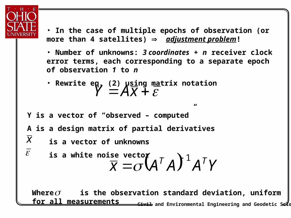
• In the case of multiple epochs of observation (or more than 4 satellites) adjustment problem!

• Number of unknowns: 3 coordinates + n receiver clock error terms, each corresponding to a separate epoch of observation 1 to n

• Rewrite eq. (2) using matrix notation

xAY

Y is a vector of “observed – computed”

A is a design matrix of partial derivatives

is a vector of unknowns

is a white noise vector

x

YAAAx TT 1

Where is the observation standard deviation, uniform for all measurements


)3(

0000

0000

0000

0000

3

2

1

333

3

222

2

111

1

0,0,

30,

30,

20,

20,

10,

10,

i

i

i

ni

i

i

i

i

ni

i

ni

i

ni

n

i

i

i

i

i

i

i

i

i

i

i

i

i

i

i

i

i

i

ni

ni

ii

ii

ii

Z

Y

X

dtc

dtc

dtc

dtc

ZYXB

ZYXB

ZYXB

ZYXB

P

P

P

P

Bj=[1 1 1 … 1]T where the number of 1 equal to the number of satellites (1,…,m) observed at epoch j (j=1,…,n)

• Rearranging terms in eq. (2) leads to a simplified form of a design matrix A, and subsequently to a normal matrix easy to handle by Gaussian elimination


• Where is a vector of unknown station coordinates [Xi Yi Zi] and matrices Ai (size (m,3)) are of the form of (1a), written for m satellites (ranges) observed at the epoch

• yj is a m-element vector of the form where j is the epoch between 1 and n

• Final system of normal equations following from eq. (3)

x

dtc

dtc

dtc

AB

AB

AB

AB

y

y

y

y

i

i

i

xnn

3

2

1

33

22

11

3

2

1

0000

0000

0000

0000

x

ji

jiP 0,0,

Rewrite eq. (3) in the following form:

VERIFY !

n

ii

Ti

nTn

T

T

n

ii

Tin

Tn

TT

nTnn

Tn

TT

TT

TT

yA

yB

yB

yB

x

cdt

cdt

cdt

AABABABA

ABBB

ABBB

ABBB

YAxAA

1

22

11

1

1

1

12211

2222

1111

00

00

00

mBB jTj

Where m is number of observations at one epoch


Dilution of PrecisionDilution of Precision

Accuracy of GPS positioning depends on:

• the accuracy of the range observables

• the geometric configuration of the satellites used (design matrix)

• the relation between the measurement error and the positioning error: pos = DOP• obs

• DOP is called dilution of precision

• for 3D positioning, PDOP (position dilution of precision), is defined as a square root of a sum of the diagonal elements of the normal matrix (ATA)-1 (corresponding to x, y and z unknowns)



PDOP is interpreted as the reciprocal value of the volume of tetrahedron that is formed from the satellite and user positions

ReceiverReceiver

Good PDOP Bad PDOPPosition error p= r PDOP, where r is the observation error (or standard deviation)



• The observation error (or standard deviation) denoted as r or obs is the number that best describes the quality of the pseudorange (or phase) observation, thus is is about 0.2 – 1.0 m for P-code range and reaches a few meters for the C/A-code pseudorange.

• Thus, DOP is a geometric factor that amplifies the single range observation error to show the factual positioning accuracy obtained from multiple observations

• It is very important to use the right numbers for r to properly describe the factual quality of your measurements.

• However, most of the time, these values are pre-defined within the GPS processing software (remember that Geomatics Office never asked you about the observation error (or standard deviation)) and user has no way to manipulate that. This values are derived as average for a particular class of receivers (and it works well for most applications!)


Dilution of PrecisionDilution of Precision• DOP concept is of most interest to navigation. If a four channel receiver is used, the best four-satellite configuration will be used automatically based on the lowest DOP (however, most of modern receivers have more than 4 channels)

• This is also an important issue for differential GPS, as both stations must use the same satellites (actually with the current full constellation the common observability is not a problematic issue, even for very long baselines)

• DOP is not that crucial for surveying results, where multiple (redundant) satellites are used, and where the Least Squares Adjustment is used to arrive at the most optimal solution

• However, DOP is very important in the surveying planning and control (especially for kinematic and fast static modes), where the best observability window can be selected based on the highest number of satellites and the best geometry (lowest DOP); check the Quick Plan option under Utilities menu in Geomatics Office


Differential GPS (DGPS)

• DGPS is applied in geodesy and surveying (for the highest accuracy, cm-level) as well as in GIS-type of data collection (sub meter or less accuracy required)

• Data collected simultaneously by two stations (one with known location) can be processed in a differential mode, by differing respective observables from both stations

• The user can set up his own base (reference) station for DGPS or use differential services provided by, for example, Coast Guard, which provides differential correction to reduce the pseudorange error in the user’s observable


By differencing observables with respect to simultaneously tracking receivers, satellites and time epochs, a significant reduction of errors affecting the observables due to:

• satellite and receiver clock biases,

• atmospheric as well as SA effects (for short baselines),

• inter-channel biases

is achieved

DGPS: Objectives and Benefits


Differential GPSDifferential GPS

• Selective Availability (SA), if it is on• Satellite clock and orbit errors• Atmospheric effects (for short baselines)

Using data from two receivers observing the same satellite simultaneously removes (or significantly decreases) common errors, including:

Base station with known location

Unknown positionSingle difference

mode


Differential GPS

• Receiver clock errors• Atmospheric effects

(ionosphere, troposphere)• Receiver interchannel bias

Using two satellites in the differencing process, further removes common errors such as:

Base station with known location

Unknown position

Double difference mode


Consider two stations i and j observing L1 pseudorange to the same two GPS satellites k and l:

lj

ljj

lj

lj

ljl

jlj

kj

kjj

kj

kj

kjk

jkj

li

lii

li

li

lil

il

i

ki

kii

ki

ki

kik

ik

i

eMbdtdtcTf

IP

eMbdtdtcTf

IP

eMbdtdtcTf

IP

eMbdtdtcTf

IP

1,1,2,1,

1,1,2,1,

1,1,2,1,

1,1,2,1,

)(

)(

)(

)(

2

1

2

1

2

1

2

1


lj

ljj

llj

lj

lj

ljl

jlj

kj

kjj

kkj

kj

kj

kjk

jkj

li

lii

lli

li

li

lil

ili

ki

kii

kki

ki

ki

kik

iki

mdtdtcNTf

I

mdtdtcNTf

I

mdtdtcNTf

I

mdtdtcNTf

I

1,1,011,11,

1,1,011,11,

1,1,011,11,

1,1,011,11,

02

1

02

1

02

1

02

1

)(

)(

)(

)(

Consider two stations i and j observing L1 phase range to the same two GPS satellites k and l:


Let’s consider differential pseudoranging first

• The single-differenced (SD) measurement is obtained by differencing two observable of the satellite k , tracked simultaneously by two stations i and j:

kij

eMij

bij

dtckij

Tf

kij

Ikij

kij

P kji 1,2,2

11,

1,

• It significantly reduces the atmospheric errors and removes the satellite clock and orbital errors; differential effects are still there (like iono, tropo and multipath, and the difference between the clock errors between the receivers)

• In the actual data processing the differential tropospheric and multipath errors are neglected, while remaining ionospheric, differential clock error, and interchannel biases might be estimated (if possible)


DGPS in Geodesy and Surveying• The single-differencedsingle-differenced measurement is obtained by differencing two observables of the satellite k , tracked simultaneously by two stations i and j:

kij

eMij

bij

dtckij

Tf

kij

Ikij

kij

P

kij

mij

dtckij

Nkij

Tf

kij

Ikij

kij

kji

kji

1,2,21

1,

1,

*1,2

11,

1,

1,1

),,(1,

*1, 11 00 jtit

kij

Nkij

N Non-integer ambiguity !


DGPS Concept, cont.• By differencing one-way observable from two receivers, i and j, observing two satellites, k and l, or simply by differencing two single differences to satellites k and l, one arrives at the double-differenced (DD) measurement:

klij

eMklij

Tf

klij

Iklij

klij

P klji 1,2

11, 1,

lij

eMij

bij

dtclij

Tf

lij

Ilij

lij

P

kij

eMij

bij

dtckij

Tf

kij

Ikij

kij

P

lji

kji

1,2,21

1,

1,2,21

1,

1,

1,

• In the actual data processing the differential tropospheric, ionospheric and multipath errors are neglected; the only unknowns are the station coordinates

Double difference

Two single differences


Differential Phase Observations

1,

*1,2

11,

1,

*1,2

11,

1,1

1,1

lij

mij

dtclij

Nlij

Tf

lij

Ilij

lij

kij

mij

dtckij

Nkij

Tf

kij

Ikij

kij

lji

kji

1,1,2

11, 1,1

klij

mklij

Nklij

Tf

klij

Iklij

klij

klji

),,(1,

*1, 11 00 jtit

kij

Nkij

N

Double difference

Two single differences

Single difference ambiguity


DGPS in Geodesy and Surveying

• By differencing one-way observable from two receivers, i and j, observing two satellites, k and l, or simply by differencing two single differences to satellites k and l, one arrives at the double-differenceddouble-differenced measurement:

ijkl

ijkl

Iijkl

fTijkl N

ijkl m

ijkl

Pijkl

ijkl

Iijkl

fTijkl M e

ijkl

ji

kl

ji

kl

, , ,

, ,

,

,

112 1 1

112 1

1 1

1


Differential Phase Observations

• Double differenced (DD) mode is the most popular for phase data processing

• In DD the unknowns are station coordinates and the integer ambiguities

• In DD the differential atmospheric and multipath effects are very small and are neglected

• The achievable accuracy is cm-level for short baselines (below 10-15 km); for longer distances, DD ionospheric-free combination is used (see the future notes for reference!)

• Single differencing is also used, however, the problem there is non-integer ambiguity term (see previous slide), which does not provide such strong constraints into the solution as the integer ambiguity for DD


Triple Difference Observable

Differencing two double differences, separated by the time interval dt provides triple-differenced measurement, that in case of phase observables effectively cancels the phase ambiguity biases, N1 and N2

ij dtkl

ij dtkl

Iij dtkl

fTij dtkl m

ji dtkl

ij dtkl

Pij dtkl

ij dtkl

Iij dtkl

fTij dtkl M

ji dtkl e

ij dtkl

, , ,,

, , , , ,

, , ,,

, , , , ,

112 1 1

112 1 1

In both equations the differential effects are neglected and the station coordinates are the only unknowns


Note: Observed phases (in cycles) are converted to so-called phase ranges (in meters) by multiplying the raw phase by the respective wavelength of L1 or L2 signals

Thus, the units in the above equations are meters!

Positioning with phase ranges is much more accurate as compared to pseudoranges, but more complicated since integer ambiguities (such as DD ambiguities) must be fixed before the positioning can be achieved

Triple difference (TD) equation does not contain ambiguities, but its noise level is much higher as compared to SD or DD, so it is not recommended if the highest accuracy is expected


St. 1

St. 2

2 (base)3 4

1

11

12 2

1

22

31

32

42

41

Positioning with phase observations: A ConceptPositioning with phase observations: A Concept


41

42

412

31

32

312

21

22

212

11

12

112

:sdifference singlefour

SD

SD

SD

SD

41

42

21

22

4212

31

32

21

22

3212

11

12

21

22

1212

DD

DD

DD

:sdifference double three

Positioning with phase observations: A ConceptPositioning with phase observations: A Concept

• Three double difference (based on four satellites) is a minimum to do DGPS with phase ranges after ambiguities have been fixed to their integer values

• Minimum of five simultaneously observed satellites is needed to resolve ambiguities

• Thus, ambiguities must be resolved first, then positioning step can be performed

• Ambiguities stay fixed and unchanged until cycle slip (CS) happens


phasesway -onefor matrix covariance diagonalgiven

DDs and SDsfor matrix covariance Find

22

41

42

412

31

32

312

21

22

212

11

12

112

TA AAσΣI

SD

SD

SD

SD

41

42

21

22

4212

31

32

21

22

3212

11

12

21

22

1212

DD

DD

DD

Covariance Matrix for Phase CombinationCovariance Matrix for Phase Combination

Four single differences Three double differences

Where A is a differencing operator matrix


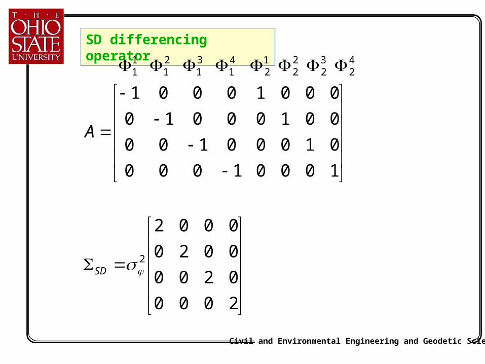
SD differencing operator

2000

0200

0020

0002

10001000

01000100

00100010

00010001

2

42

32

22

12

41

31

21

11

SD

A


422

242

224

10101010

01100110

00110011

2

42

32

22

12

41

31

21

11

SDD

A

DD differencing operator

• Thus DD covariance matrix is a full matrix for one epoch

• For several epochs – it will be a block diagonal matrix


• We have talked so far about single, double and triple differences of GPS observable (predominantly phase), which are nothing else but linear combinations of direct measurements. These linear combinations become very handy in removal (or at least significant reduction) of various error sources and nuisance parameters, making positioning process rather simple (at least for short baselines). Keep in mind that the covariance matrix becomes more complicated, but that is a small price to pay for a limited number of unknowns offered in double differencing!

• There are, however, even more “advanced” linear combinations whose specific objectives would be to further eliminate some errors that might still be present in differential form in the, for example, double difference equation, and to simplify (or enable) certain actions – such as ambiguity resolution (we know that ambiguities must be resolved before we can do positioning with GPS phase observations).

• So, let’s take a look at some of the most useful linear combinations (you can create any combination you like, the point is to make it in a smart way so that it would make your life easier!


Useful linear combinationsUseful linear combinations

• Created usually from double-differenced phase observations

• Ion-free combination based on L1 and L2 observable eliminates ionospheric effects (actually, the first order only)

• Ion-only combination based on L1 and L2 observable, (useful for cycle slip tracking) eliminates all effects except for the ionosphere, thus can be used to estimate the ionospheric effect

• Widelane – its long wavelength of 86.2 cm supports ambiguity resolution; based on L1 and L2 observable


Ionosphere-free combinationIonosphere-free combination

• ionosphere-free phase measurement

1 2 1 1 2 2

1 1 1 2 2 2 1 1 2 2

,

T N N

11

2

1

2

2

2

22

2

1

2

2

2

f

f f

f

f f

• similarly, ionosphere-free pseudorange can be obtained

• The conditions applied are that sum of ionospheric effects on both frequencies multiplied by constants to be determined must be zero; second condition is for example that sum of the constants is 1, or one constant is set to 1 (verify!)

221

22

12,1 Rf

fRR


Ionosphere-free combinationIonosphere-free combination

0

1

0

22

22

121

1

21

22

221

1

f

I

f

I

f

I

thus

f

I

f

I

22

21

22

2

22

21

21

1

22

22

21

21

22

1

:

1

:

ff

f

ff

f

finally

fff

ff

gsimplifyin

Take the ionospheric terms on L1 and L2 and assume that they meet the following conditions (where 1 and 2 are the “to be determined” coefficients defining the iono-free combination:

However, we only considered the 1st order ionospheric term here!


Estimated ionospheric group delay for GPS signal (see the table)• The first order effects are most significant• In the phase/range equation we use only 1st order ionospheric terms• Thus the iono-free combination is in fact only ion 1st order iono-free

L1 L2 Residual Range Error

First Order: 1/f 2

16.2 m 26.7 m 0.0

Second Order: 1/f 3

~ 1.6 cm ~ 3.3 cm ~ -1.1 cm

Third Order: 1/f 4

~ 0.86 mm ~ 2.4 mm ~ -0.66 mm

Calibrated 1/f 3

Term Based on a Thin Layer Ionospheric Model

~ 1-2 mm

The phase advance can be obtained from the above table by multiplying each number by -1, -0.5 and -1/3 for the 1/f 2, 1/f 3 and 1/f 4 term, respectively


index refractive phase 2

1

signal) GPS code assuch waves,of (groupindex refractive group 2

1

33

22

33

22

f

c

f

cn

f

c

f

cn

ph

gr

• Integration of the refractive index renders the measured range, and the ionospheric terms for range and phase (see earlier notes)

• Denoting the 1st and 2nd order iono term as follows (after the integration, in cycles; a and be are constants):

• We can now consider forming so-called iono-free combination phase equation, but including the second order iono term (see the enclosed hand-out)

• Based on the L1 and L2 frequencies, and assuming the proposed third GPS frequency called L5, we can form two iono-free combinations, and combine them further to derive a 2nd order ion-free linear combination (future!)

2kkk

ionok

f

b

f

a


• Notice that the two 1st order iono-free combinations and

used here, were derived under the assumption that 1 was set to 1, as opposed to

our condition used earlier that 1+2=1 (see also the handout)

• We can now derive the 2nd order ionospheric term as follows (by using the above ion-free combinations for the ionospheirc terms only, including the 2nd order, as shown on the slide above):

Now, the general form of the 2nd order iono-free combination is as follows:

Where the inospheric terms above are used to estimate the n1 and n2 under the assumption that the final iono term in the linear combination will disappear

2nd order ion-free combination

251

5112

1

21 ][][ n

f

fn

f

f ijijijij

211

2

2

2

1

1 *)60/17(

f

b

f

fionoiono

2

11

5

5

5

1

1 *)115/39(

f

b

f

fionoiono

ijij

f

f2

1

21 ijij

f

f5

1

51


Assuming n1 =1 and using the conditions above we can write:

And finally arrive at the n2 value for this combination:

))(1/())(1(3

1

2

12 f

f

f

fn

2nd order ion-free combination

251

512

1

21 ][][ n

f

f

f

f ijijijij thus

Represents the 2nd order ionosphere-free linear combination (future!)

Notice the non-integer ambiguity!

0)*)115/39(

(*)60/17(

21

221

f

bn

f

b


Other useful linear combinationsOther useful linear combinations

• widelanewidelane where is in cycles

the corresponding wavelength

klwij

klij

klw

klij

klijkl

ijkl

wij NNTf

f

f

Iij ,2,

2

1, 1,2

1

w cm 1 2

2 1

86 2.

ionospheric-onlyionospheric-only (geometry-free) combination is obtained by differencing two phase ranges [m] belonging to the frequencies L1 and L2

w 1 2

[meter]

[meter]kl

onlyionoijklij

klij

klij

klij

klij

klonlyionoij NN

ff

ffI

,2,21,12

22

1

22

21

2,1,, )(

Non-integer ambiguity!


WidelaneWidelane

2

12

121,12

12

12

1

22

121

1221

21

12

1221

22

2121

1221

21

12

122

2

21

2121

1221

21

12

22

222

212

111

121

11

11

11

f

f

f

ITNN

f

ITNN

f

ITNN

f

f

f

ITNN

T

f

IN

T

f

IN

ww

• Difference between phase observable on L1 and L2 (in cycles)

w cm 1 2

2 1

86 2.

Widelane in [m]

Widelane wavelength


• Phase observable, although very accurate, must have an initial integer ambiguity resolved before it can be used for positioning.

• Any time we loose lock to the satellite or so called cycle slip happens, we need to re-establish the ambiguity value before we can continue with positioning!

• What is a cycle slip and what do we do to fix it?

• The ambiguity resolution algorithm is coming soon!


Cycle Slips• Sudden jump in the carrier phase observable by an integer number of cycles

• All observations after CS are shifted by the same integer amount

• Due to signal blockage (trees, buildings, bridges)

• Receiver malfunction (due to severe ionospheric distortion, multipath or high dynamics that pushes the signal beyond the receiver’s bandwidth)

• Interference

• Jamming (intentional interference)

• Consequently, the new ambiguities must be found


time

Initial ambiguity

Phase observations with cycle slip at epoch t0

t0

New ambiguity

Cycle slips must be found and fixed before we can use the data (at the given epoch and beyond) for positioning


Cycle Slip Detection and Fixing• Use ionosphere-only combination

• under normal conditions, ionosphere changes smoothly with time, so any abrupt changes in ionosphere-only combination indicates cycle slip

• Single, double or triple difference residuals can be tested

• Phase and range combination can also be used, however, this will not detect small cycle slips due to large noise on pseudorange

• Receivers try to resolve CS using extrapolation, flag the data with possible cycle slips

ij iono only

kl

ij

kl

ij

kl

ij

kl

ij

kl

ij

kl

ij iono only

klIf f

f fN N, , , , , ,( )

1 2

1 2

1 2

1 1 2 2

21

1,1,1,1, 2f

INR j

iij

iji


Cycle Slip Detection and Fixing

• Cycle slips can be located by comparing either one of the listed quantities between two consecutive epochs (jump occurs)

• Also, a time series of the testing quantity can be examined (1st, 2nd, 3rd and 4th differences of the series of testing quantity)

• To find the correct size of CS the curve fit to the testing quantity is performed before and after CS

• Shift between the curves indicates the cycle slip amount

• Kalman filter prediction can also be used (predicted value – observed value indicates the size of CS)

• The testing quantities are then corrected by adding the size of CS to all the subsequent quantities


Cycle Slip Detection and Fixing, Final Solution

• A good method is to carry out a triple difference solution first

• Since only one TD is affected it can be treated as a blunder, and a least squares solution can still be obtained

• The residuals of converged TD solution indicate the size of cycle slips

• Before using DD for the final solution, DD should be corrected for CS

• Least squares solution with non-integer ambiguities (float solution)

• Fix ambiguities

• Final Least squares solution with integer ambiguities (constraints)


• Differential Global Positioning System (DGPS) is a method of providing differential corrections to a GPS receiver in order to improve the accuracy of the navigation solution.

• DGPS corrections originate from a reference station at a known location. The receivers in these reference stations can estimate errors in the GPS observable because, unlike the general population of GPS receivers, they have an accurate knowledge of their position.

• As a result of applying DGPS corrections, the horizontal accuracy of the system can be improved from 10-15 m (100m under SA), 95% of the time, to better than 1m (95% of the time).

Differential GPS (DGPS) ServicesDifferential GPS (DGPS) Services


Differential GPS (DGPS) Services

• There exists a reference station with a known location that can determine the range corrections (due to atmospheric, orbital and clock errors), and transmit them to the users equipped with proper radio modem.

• The DGPS reference station transmits pseudorange correction information for each satellite in view on a separate radio frequency carrier in real time.

• DGPS is normally limited to about 100 km separation between stations.

• Improves positioning with ranges by 100 times (to sub-meter level)


Some DGPS Services

• Starfix II OMNI-STAR (John E. Chance & Assoc, Inc.)

• U.S. Coast Guard• Federal Aviation Administration• GLOBAL SURVEYOR™ II NATIONAL,

Natural Resources Canada• Differential Global Positioning

System (DGPS) Service, AMSA, Australia


Wide Area Differential GPS Wide Area Differential GPS (WADGPS)(WADGPS)

• Differential GPS operation over a wider region that employs a set of monitor stations spread out geographically, with a central control or monitor station.

• WADGPS uses geostationary satellites to transmit the corrections in real time (5-10 sec delay).

• For example: OMNISTAR, Differential Corrections Inc., WAAS (FAA-developed Wide Area Augmentation System)


Atmospheric layer

A Schematic of the WAASA Schematic of the WAAS


• The WAAS improves the accuracy, integrity, and availability of the basic GPS signals

• A WAAS-capable receiver can give you a position accuracy of better than three meters, 95 percent of the time

• This system should allow GPS to be used as a primary means of navigation for enroute travel and non-precision approaches in the U.S., as well as for Category I approaches to selected airports throughout the nation

• The wide area of coverage for this system includes the entire United States and some outlying areas such as Canada and Mexico.

• The Wide Area Augmentation System is currently under development and test prior to FAA certification for safety-of-flight applications.

WAASWAAS


• Total correction estimation is accomplished by the use of one or more GPS Base Stations that measure the errors in GPS pseudo-ranges to all satellites in view, and generate corrections

• Subsequently, the corrections are sent to the users

• Thus, real-time DGPS always involves some type of wireless transmission system (one-way, i.e., the user does not send any info back)

• VHF systems for short ranges (FM Broadcast)

• low frequency transmitters for medium ranges (Beacons)

• geostationary satellites (OmniSTAR) for coverage of entire continents.

• So, we know how to communicate with DGPS (or WADGPS) services, but how does the system generate the actual corrections, and how do they get customized for the user’s location?

WADGPS: operational aspectsWADGPS: operational aspects


• A GPS base station tracks all GPS satellites that are in view at its location.

• Given the precise surveyed location of the base station antenna, and the location in space of all GPS satellites at any time from the ephemeris data (navigation message broadcast from all GPS satellites), an expected (or “theoretical”)range to each satellite can be computed for any time

• The difference between that computed range and the measured range is the range error

• If that information can quickly be transmitted to other nearby users, they can use those values as corrections to their own measured GPS ranges to the same satellites (DGPS)

• In case of WADGPS, the local base stations send their corrections to the master station that is responsible for the communication via the geostationary satellite

• Thus, the satellite would receive and disseminate a set of corrections coming from all the WADGPS network base stations



How does the user get customized/optimized correction?

• For example, OmniSTAR user sets receive these packets of data from the satellite transponder (an exact duplicate of the data as it was generated at each base station)

• Next, the atmospheric errors must be corrected. Every base station automatically corrects for atmospheric errors at its location, because it is a part of the overall range error; but the user is likely to be not at any of those locations, so the corrections are not optimized for the user.

• Also, the OmniSTAR system has no information about each individual's location So, if these corrections are to be automatically optimized for each user's location, then it must be done in each user's Omnistar.



• For this reason, each OmniSTAR user set must be given an approximation of its location (from the GPS receiver being a part of OmniSTAR set)

• Given that information, the OmniSTAR user set can use a Model to compute and remove most of the atmospheric correction contained in satellite range corrections from each Base Station message, and substitute a correction for its own location.

• After the OmniSTAR processor has taken care of the atmospheric corrections, it then uses its location - versus the eleven base station locations, in an inverse distance-weighted least-squares solution.

• The output of that least-squares calculation is a synthesized Correction Message that is optimized for the user's location.

• This technique of optimizing the corrections for each user's location is called the Virtual Base Station Solution



• All WADGPS systems generate range and range rate correction

• The range correction is an absolute value, in meters, for a given satellite at a given time of day.

• The range-rate term is the rate that correction is changing, in meters per second. That allows GPS users to continue to use the "correction, plus the rate-of-change" for some period of time while waiting for a new message.

• In practice, OmniSTAR would allow about 12 seconds in the "age of correction" before the error from that term would cause a one-meter position error.

• OmniSTAR transmits a new correction message every two and one/half seconds, so even if an occasional message is missed, the user's "age of data" is still well below 12 seconds.



OmniSTAR's unique "Virtual Base Station" technology generates corrections optimized for the user's location. OmniSTAR receivers output both high quality RTCM-SC104 (Radio Technical Commission for Maritime Services) Version 2 corrections and differentially corrected Lat/Long in NMEA format (National Marine Electronics Association).


OmniSTAR receiver


Radio Modems

This file can be found on the course web page: geodesy.eng.ohio-state/course/gs609

Documents

Transcript of This file can be found on the course web page: geodesy.eng.ohio-state/course/gs609