This article was originally published in Treatise on...
46
This article was originally published in Treatise on Geophysics, Second Edition, published by Elsevier, and the attached copy is provided by Elsevier for the author's benefit and for the benefit of the author's institution, for non-commercial research and educational use including without limitation use in instruction at your institution, sending it to specific colleagues who you know, and providing a copy to your institution’s administrator. All other uses, reproduction and distribution, including without limitation commercial reprints, selling or licensing copies or access, or posting on open internet sites, your personal or institution’s website or repository, are prohibited. For exceptions, permission may be sought for such use through Elsevier's permissions site at: http://www.elsevier.com/locate/permissionusematerial Schmitt D.R Geophysical Properties of the Near Surface Earth: Seismic Properties. In: Gerald Schubert (editor-in-chief) Treatise on Geophysics, 2 nd edition, Vol 11. Oxford: Elsevier; 2015. p. 43-87.
Transcript of This article was originally published in Treatise on...

This article was originally published in Treatise on Geophysics, Second Edition, published by Elsevier, and the attached copy is provided by Elsevier for the author's benefit and for the benefit of the author's institution, for non-commercial research and educational use including without limitation use in instruction at your institution, sending it to specific colleagues who you know, and providing a copy to your institution’s administrator.
All other uses, reproduction and distribution, including without limitation commercial reprints, selling or licensing copies or access, or posting on open internet sites, your
personal or institution’s website or repository, are prohibited. For exceptions, permission may be sought for such use through Elsevier's permissions site at:
http://www.elsevier.com/locate/permissionusematerial
Schmitt D.R Geophysical Properties of the Near Surface Earth: Seismic Properties. In: Gerald Schubert (editor-in-chief) Treatise on Geophysics, 2nd edition, Vol 11. Oxford:
Elsevier; 2015. p. 43-87.

Tre
Author's personal copy
11.03 Geophysical Properties of the Near Surface Earth: Seismic PropertiesDR Schmitt, University of Alberta, Edmonton, AB, Canada
ã 2015 Elsevier B.V. All rights reserved.
11.03.1 Introduction 4411.03.2 Basic Theory 4511.03.2.1 Hooke’s Constitutive Relationship and Moduli 4511.03.3 Mineral Building Blocks 4711.03.3.1 Elastic Properties of Minerals 4711.03.3.2 Bounds on Isotropic Mixtures of Anisotropic Minerals 4811.03.3.3 Isothermal Versus Adiabatic Moduli 4911.03.3.4 Effects of Pressure and Temperature on Mineral Moduli 5111.03.3.5 Mineral Densities 5111.03.4 Fluid Properties 5311.03.4.1 Phase Relations for Fluids 5411.03.4.2 Equations of State for Fluids 5411.03.4.2.1 Ideal gas law 5611.03.4.2.2 Adiabatic and isothermal fluid moduli 5611.03.4.2.3 The van der Waals model 5711.03.4.2.4 The Peng–Robinson EOS 5711.03.4.2.5 Correlative EOS models 5811.03.4.2.6 Determining Kf from equations of state 5811.03.4.3 Mixtures and Solutions 5911.03.4.3.1 Frozen mixtures 5911.03.4.3.2 Miscible fluid mixtures 6011.03.5 The Rock Frame 6511.03.5.1 Essential Characteristics 6511.03.5.2 The Pore-Free Solid Portion 6611.03.5.3 Influence of Porosity 6711.03.5.4 Influence of Crack-Like Porosity 6911.03.5.5 Pressure Dependence in Granular Materials 7211.03.5.6 Implications of Pressure Dependence 7311.03.5.6.1 Stress-induced anisotropy (acoustoelastic effect) 7311.03.5.6.2 Influence of pore pressure 7411.03.6 Seismic Waves in Fluid-Saturated Rocks 7411.03.6.1 Gassmann’s Equation 7511.03.6.2 Frequency-Dependent Models 7611.03.6.2.1 Global flow (biot) model 7711.03.6.2.2 Local flow (squirt) models 7811.03.7 Empirical Relations and Data Compilations 7811.03.8 The Road Ahead 81Acknowledgments 81References 81
GlossaryAdiabat An adiabatic path in P–V–T space.
Adiabatic A thermodynamic process in which no heat is
allowed to transfer into or out of the system. The local
compression and rarefaction and corresponding increase
and decrease of both pressure and temperature of a material
as compressional wave passes are assumed to be an adiabatic
process.
Anisotropy The condition in which the physical properties
of a material will depend on direction.
Aspect ratio x (dimensionless) In the context of crack-like
porosity, this refers to the aperture width of the crack to its
length.
Bulk modulus K (Pa) Also called the incompressibility.
Ameasure of the resistance of a material to deformation for a
given change in pressure.
Compliances Sij (Pa�1) The elastic mechanical parameters
that generally relate stresses to strains.
Compressibility (Pa�1) Inverse of the bulk modulus.
atise on Geophysics, Second Edition http://dx.doi.org/10.1016/B978-0-444-538
Treatise on Geophysics, 2nd editio
02-4.00190-1 43n, (2015), vol. 11, pp. 43-87
44 Geophysical Properties of the Near Surface Earth: Seismic Properties
Author's personal copy
Cricondenbar For fluid mixtures. The greatest pressure at
which both liquid and vapor phases can coexist. Above the
cricondenbar, the mixture must be either a liquid or a
supercritical fluid phase.
Critical point For pure fluids, a point in P–V–T space at
which the liquid–vapor phase line terminates. The fluid will
be in the supercritical state for pressures and temperatures
above the critical pressure Pc and temperature Tc. At the
critical point the fluid will have the critical specific volume
Vc or equivalently the critical density rc¼M/Vc, where M is
the chemical molecular weight.
Cricondentherm For fluid mixtures. The greatest
temperature at which both liquid phase and vapor phase can
still coexist. Above this temperature, the fluid will be either
vapor or supercritical fluid phase.
Density r (kg m�3) Mass per unit volume.
Equation of state A theoretical or empirical function or set
of functions that describes the material’s specific volume as a
function of pressure and temperature.
Hooke’s law The mathematical relationship between stress
and strain via the elastic stiffnesses or conversely the strains
and the stresses via the elastic compliances.
Isentropic A thermodynamic process in which the entropy
of the system remains constant. A reversible adiabatic
process is also isentropic.
Isochor A thermodynamic path in P–V–T space in
which the specific volume Vm or the density r remains
constant.
Isotherm A thermodynamic path in P–V–T space in
which the temperature T remains constant. These are
often the conditions employed in conventional
measurements of fluid properties particularly in the
petroleum industry.
Lame parameters l and m (Pa). The two elastic parameters
relating stresses to strains in the Lame mathematical
formulation of Hooke’s law.
Poisson’s ratio n (dimensionless) The negative of the ratio
between the radial and the axial strains induced by an axial
stress.
Polycrystal A material that is a mixture of mineral crystals
and that, often, is assumed to be free of pores. The properties
of the polycrystal are then taken to be representative of those
for the solid portion of the rock.
Pseudocritical point For fluid mixtures, a point in P–V–T
space where the bubble and dew lines meet. This point
depends on the composition of the mixture and occurs at
the pseudocritical pressure PPC and temperature TPC.
Saturated The condition where the pore space of the rock is
filled with fluids.
Saturation The fraction of the pore space that is filled with a
given fluid. If only one fluid fills the pore volume, it will have
a saturation of 1. If the pore volume is equally filled with two
different fluids, they each will have a saturation of 0.5.
Shear modulus m (Pa) The elastic mechanical parameter
relating shear stress to shear strain.
Stiffness Cij (Pa) The elastic mechanical parameters that
generally relate strains to stresses.
Strain eij or gij (dimensionless) Measures of the
deformation of a material.
Stress sij or tij (Pa) The ratio of an applied force to the area
over which it is applied. Normal stresses sij are directedperpendicularly to the surface. Shear stresses tij are directedalong the plane of the surface.
Supercritical The condition for a fluid encountered in P–V–T
space in which it is no longer considered a liquid or a vapor
(gas) but a fluid with the characteristics of both. For single-
component fluids, the supercritical phase exists above the
critical point at the critical pressure Pc and temperature Tc.
Young’s modulus E (Pa) Also often referred to as the
modulus of elasticity. The elastic mechanical parameter
relating the linear axial strain induced to the applied axial
normal stress.
Treatise on Geophysics, 2nd edition,
11.03.1 Introduction
Geophysicists measure the spatial and temporal variations in
electromagnetic, magnetic, and gravitational potentials and
seismic wave fields in order to make inferences regarding the
internal structure of the Earth in terms of, respectively, its
electrical resistivity (See Chapters 2.25, 11.04, 11.08, and
11.10), its magnetism (See Chapters 2.24, 5.08, 11.05,
11.11), its density (See Chapter 3.03, 11.05, 11.12), and its
elasticity (See Chapters 1.26 and 2.12). In seismology the
most basic observation is that of a seismic wave’s travel time
from its source to the point of measurement. Seismologists
continue to develop increasingly sophisticated analyses to con-
vert this basic observation into seismic velocities from which
the Earth’s structure may be deduced. This holds true for the
simplest 1-D seismic refraction analysis to the most compli-
cated modern 3-D whole Earth tomogram. The influence of
this velocity is not so directly apparent in seismic reflection
profiles, but proper imaging depends critically on solid knowl-
edge of the in situ seismic velocity structure. Indeed, as
computational power grows, the differences between inversion
and advanced prestack migration in imaging will become less
distinct.
Velocity, as it is used in the geophysical community for
wave speed, would certainly first come to a geophysicist’s
mind as a seismic property. It is also the seismic property that
is most often used to infer lithology. Liberally, compressional
wave velocities that can exist in crustal materials can range
from a few hundred meters per second in air-saturated uncon-
solidated sediments to upward of 8 km s�1 for high-grade
metamorphosed rocks at the top of the mantle. Typically
then, within a given geologic context, the velocities themselves
or additional parameters derived from them such as the
compressional/shear wave speed ratio VP/VS, Poisson’s ratio
n, or the seismic parameter ’¼ VP2� 4VS
2/3 are useful indicators
of lithology. Unfortunately, the seismic velocities of any given
lithology are not unique. Seismic velocities are affected by
numerous factors such as mineralogical composition, texture,
porosity, fluids, confining stress, pressure, and temperature, all
of which contribute by differing degrees to the value of the
(2015), vol. 11, pp. 43-87

Geophysical Properties of the Near Surface Earth: Seismic Properties 45
Author's personal copy
observed wave speed. Seismic anisotropy, being the variation
of the wave speeds with direction of propagation through the
medium, may also need to be included (Chapter 2.20). With
attenuation, even the frequency at which the observation is
made should be considered.
With a particular focus on the porous and fluid-filled Earth
materials near the Earth’s surface, the purpose of this contri-
bution is to review ‘seismic properties.’ To most workers, this
will again mean the measurable ‘seismic velocity.’ Such veloc-
ities are what we, as remote observers, can measure. More
fundamentally, however, the seismic velocities are a manifes-
tation of the competition between a material’s internal forces
(represented in a continuum via the elastic moduli) and inertia
(through density). Without derivation, the relationships
between the compressional P and S waves and the material’s
moduli and bulk density r are
VP ¼ffiffiffiffiffiffiffiffiffiffiffiffiffiffiffiffiffiffiK +4m=3
r
s[1]
VS ¼ffiffiffimr
r[2]
where K and m are the bulk and shear moduli for an isotropic
medium, respectively. As fluids cannot support a shear stress,
their m¼0 and eqn [1] reduces to the simpler longitudinal
elastic wave of speed VL
VL ¼ffiffiffiffiK
r
s[3]
first derived by Newton and thermodynamically corrected by
Laplace. Care must be exercised in the choice of K particularly
for fluids; much of the task of this contribution will not be in
the examination of the wave speeds so much as attempting to
understand the material’s elastic moduli.
Later, when discussing a fluid-filled porous rock, the K and
m to be used in eqns [1] and [2] will necessarily be those of the
bulk mixture of solids and fluids and will appropriately be
denoted Ksat and msat, respectively.A given wave speed depends on the ratio between the
moduli and density. One cannot understand the meaning of
an observed seismic velocity, nor calculate it, without sufficient
knowledge of these underlying moduli and density. Not sur-
prisingly, then, the complexity of the physics needed to
describe a wave velocity increases with the number of the
material’s characteristics considered. In particular, the intro-
duction to the problem of porosity and mobile fluids multi-
plies the number of free parameters that can influence the
material’s moduli and density. Properly describing a near-
surface material is substantially more difficult than trying to
predict variations in, for example, the Earth’s mantle where
excursions of only a few percent are considered large!
This review is also carried out from the perspective of rock
physics, the factors affecting wave speeds and the models used
to predict them are presented. This is all done from the
viewpoint of an experimentalist concerned with attempting
to test such theories. That said, it must be recognized that
often, one cannot have all of the information necessary, nor
Treatise on Geophysics, 2nd editio
are the models sufficiently sophisticated, to properly predict a
given velocity. This will more often than not be the case in
seismic investigations of the near surface for resource explo-
ration or engineering and environmental characterization. As
such, at the end, a number of empirical relationships are also
described. The basics of elasticity, anisotropy, and
poroelasticity are briefly covered in order to set the stage for
understanding how wave speeds relate to moduli. In attempting
to understand the seismic properties of a fluid-saturated crustal
rock, one must first have some understanding of the physical
properties of the rock’s constituent solid minerals, its saturating
fluids, and finally its ‘frame.’ Minerals and fluids are the basic
components in rocks in the upper crust and their behavior first
must be studied. This is followed by a review of the factors
affecting the rock’s frame properties. Finally, these different
components affecting rock properties are then integrated using
various theories to arrive at estimates of the seismic properties.
However, one may not always have available sufficient informa-
tion to allow for the calculation of the physical properties, and
for this case, a number of empirical relations and references to
published compilations of observed results are provided. Lack of
space restricts delving in detail into the range of issues related to
seismic properties, so I conclude with some thoughts about the
topics that will be important in the coming decade. A short
glossary of terms that are not normally encountered in the
geophysical literature is also provided.
11.03.2 Basic Theory
Any understanding of the propagation of mechanical waves
rests on basic elasticity theory. The number of texts on this
topic is large and little is to be gained here by repeating the
basic concepts of stress and strain, the development of
Hooke’s law, or the construction of the wave equations link-
ing elasticity to wave velocities. I assume the reader will have
some basic understanding of elasticity. Some recommended
texts covering the basic governing equations at different levels
of sophistication include Bower (2010), Fung (1965), and
Tadmor et al. (2012). Stein and Wysession (2002) gave a
particularly cogent exposition of both isotropic elasticity
and the solution to the wave equation particularly as it relates
to seismology. Auld (1990) provided an excellent advanced
overview of elasticity with good emphasis on elastic
anisotropy; the notation styles employed here follow largely
from this text. For understanding of more complicated
materials, the essentials of poroelasticity can be found in
Wang (2000), Bourbie et al. (1987), and Gueguen and
Bouteca (2004); of anelasticity in Lakes (2009) and
Carcione (2007); and of hyperelasticity (nonlinear elasticity)
in Holzapfel (2000). These texts will well cover the details,
and only the necessary definitions of moduli within the Voigt
representation of Hooke’s law are provided.
11.03.2.1 Hooke’s Constitutive Relationship and Moduli
In this contribution, we assume all strains are infinitesimal and
describe to the first order the material’s deformation via the
strain tensor e
n, (2015), vol. 11, pp. 43-87

Vo
Vo (1 + q )
szz
szz
wo
wo (1 + exx)
l o(1
+e z
z)
(a)
(b)
(c)
P
x
y
z
txy
gxyl o
Figure 1 Illustration of the three basic deformations that allow theisotropic elastic moduli to be described. The original dimensions of theobject are in light red with the deformed version in transparent purple.(a) Change in volume yVo upon application of uniform pressure Pdefining the bulk modulus K¼�P/y, there is no change in shape. (b)Change in the length loEyy and width woExx upon application of a uniaxialstress syy defining the Young’s modulus E¼syy/Eyy and Poisson’s ration¼�Exx/Eyy. Both the shape and volume change and (c) the change inshape described by the angle g¼2Exy upon application of a simpleshear stress txy defining the shear modulus m¼txy/Exy. There is nochange in volume.
46 Geophysical Properties of the Near Surface Earth: Seismic Properties
Author's personal copy
E x, y, zð Þ¼Exx Exy ExzEyx Eyy EyzEzx Ezy Ezz
264
375
¼
@ux@x
1
2
@ux@y
+@uy@x
� �1
2
@ux@z
+@uz@x
� �1
2
@uy@x
+@ux@y
� �@uy@y
1
2
@uy@z
+@uz@y
� �1
2
@uz@x
+@ux@z
� �1
2
@uz@y
+@uy@z
� �@uz@z
2666666664
3777777775
[4]
where the displacement of the particle originally at (x, y, z) is
given by the vector u¼uxi+uyj+uzk. Forces within the mate-
rials are defined by the stress tensor s:
s x, y, zð Þ¼sxx txy txztyx syy tyztzx tzy szz
24
35 [5]
where normal and shear stresses are represented by sii and tij,respectively. Hooke’s law is the linear constitutive relationship
between strain equation [4] and stress equation [5]. The sim-
plest case of an isotopic medium is most commonly assumed
in studies of wave propagation. In this case, Hooke’s law may
be written in the abbreviated Voigt notation as using the math-
ematical simplifications afforded by the use of the Lame
parameters l and m :
sxxsyyszztyztzxtxy
26666664
37777775¼
l+ 2m l l 0 0 0l l +2m l 0 0 0l l l+ 2m 0 0 00 0 0 m 0 00 0 0 0 m 00 0 0 0 0 m
26666664
37777775
ExxEyyEzz2Eyz2Ezx2Exy
26666664
37777775
[6]
The reader should take note of the pattern relating the
tensors of eqns [4] and [5] to the stress and strain vectors of
the Voigt abbreviated notation of eqn [6] in which the shear
strains are multiplied by the awkward factor of 2. The Lame
formulation is mathematically elegant and simple. This sim-
plicity comes with some cost, however, in that l cannot be
directly measured in a simple experiment. In contrast, the
second Lame parameter m is the shear modulus, which is the
simple ratio between an applied shear stress t and the resulting
shear strain gij¼2Eij, a value that can readily be experimentally
measured (Figure 1(c)).
Two other important moduli in isotropic media are Young’s
modulus E and the already introduced bulk modulus K. These
can be found by conducting simple experiments with clear
physical interpretations. E is the ratio between an applied
uniaxial stress and its corresponding resulting coaxial linear
strain (Figure 1(b)). K is the ratio between an applied uniform
(hydrostatic) pressure P and the consequent volumetric strain
y¼ Exx+ Eyy+ Ezz. Poisson’s ratio n is not a modulus but it too is
an important and popular measure of a material’s deformation
under stress. It is simply the negative of the ratio between the
lateral Exx and axial Eyy strains observed during the same test
used to measure E (Figure 1(b)).
E, K, l, m, or n can be calculated if any of the other two
moduli or parameters are known; extensive conversion tables
are readily found (e.g., Birch, 1961; Mavko et al., 2003). Some
of these relations are, for convenience,
Treatise on Geophysics, 2nd edition,
E¼ 9Km3K + m
K ¼ l+2m=3
m¼ 3
2K�lð Þ
n¼ 3K�E
6K
[7]
In the case of a liquid, m¼0 and l can be assigned a physical
interpretation as it collapses to the bulk modulus K.
Although we will not be directly addressing issues of seis-
mic reflectivity here, one can also consider the acoustic imped-
ances Zi¼riVi, where i indicates either the P or the S wave, as a
physical property in their own right.
Most of the theoretical models that will follow attempt to
develop expressions for K and m. With this in mind, Hooke’s
(2015), vol. 11, pp. 43-87

2666666664
Geophysical Properties of the Near Surface Earth: Seismic Properties 47
Author's personal copy
law (eqn [6]) may alternatively be expressed less elegantly but
more physically as
sxxsyyszztyztzxtxy
26666664
37777775¼
K +4
3m K�2
3m K�2
3m 0 0 0
K�2
3m K +
4
3m K�2
3m 0 0 0
K�2
3m K�2
3m K +
4
3m 0 0 0
0 0 0 m 0 0
0 0 0 0 m 0
0 0 0 0 0 m
266666666666664
377777777777775
ExxEyyEzz2Eyz2Ezx2Exy
26666664
37777775
[8]
A comparison of eqns [1] and [7] also allows the moduli to
be written in terms of the wave speeds as
m¼ rV2S ,
K ¼ r V2P �
4
3V2S
� �,
n¼ 1
2
V2P �2V2
S
V2P �V2
S
� � [9]
11.03.3 Mineral Building Blocks
11.03.3.1 Elastic Properties of Minerals
The majority of seismological studies assume that the elastic
responses of Earth materials behave according to eqn [6]. In
reality, however, isotropy is the exception; all minerals and
most rocks are elastically anisotropic. We introduce this
topic early as it is key to understanding how we arrive at the
physical properties of the minerals that constitute the rocks.
To include this anisotropy, eqn [8] may more generally be
rewritten as
sxxsyyszztyztzxtxy
3777777775¼ s¼
C11 C12 C13 C14 C15 C16
C21 C22 C23 C24 C25 C26
C31 C32 C33 C34 C35 C36
C41 C42 C43 C44 C45 C46
C51 C52 C53 C54 C55 C56
C61 C62 C63 C64 C65 C66
2666666664
3777777775¼
ExxEyyEzz2Eyz2Ezx2Exy
2666666664
3777777775¼ c½ �E [10]
where each of the matrix components Cij is called the elastic
stiffnesses. More formally, eqn [10] condenses the expression
of Hooke’s law through the fourth-order tensor components
sij¼ cijklEkl with the condensed subscripts following the rules:
xx!1, yy !2, zz ! 3, yz !4, xz!5, and xy ! 6 [11]
and with the full stiffness matrix represented by [c]. E and srepresent the corresponding stress and strain vectors, respec-
tively, within this abbreviated notation. Further, Cij¼Cji mak-
ing [c] symmetrical such that there are at most 21 independent
elastic stiffnesses. The total number depends on the degree of
symmetry of the system varying from only 2 for the isotropic
case just shown to the full 21 for the least symmetrical triclinic
crystals as will be discussed shortly. Conversely, the strains can
be written in terms of the applied stresses using the elastic
compliances Sij with their matrix similarly represented by [s]
Treatise on Geophysics, 2nd editio
ExxEyyEzz2Eyz2Ezx2Exy
26666664
37777775¼ E¼
S11 S12 S13 S14 S15 S16S21 S22 S23 S24 S25 S26S31 S32 S33 S34 S35 S36S41 S42 S43 S44 S45 S46S51 S52 S53 S54 S55 S56S61 S62 S63 S64 S65 S66
26666664
37777775
sxxsyyszztyztzxtxy
26666664
37777775¼ s½ �s [12]
The author takes no responsibility for the fact that conven-
tionally [s] and [c] are used to, respectively, denote the com-
pliances and the stiffnesses. Regardless, the Voigt form is
particularly useful because
c½ � ¼ s½ ��1 [13]
where the superscript ‘�1’ indicates the matrix inverse opera-
tion (Auld, 1990). We note that an important property of the
tensor (in its abbreviated form here) is its transformation upon
change of the basis coordinate system. The mathematics
describing this is beyond the needs of this contribution but
Walker and Wookey (2012) provided convenient MATLAB®
codes to carry out these otherwise tedious calculations.
Using this form, eqn [8] for the isotropic case is
sxxsyyszztyztzxtxy
26666664
37777775¼
C11 C12 C12 0 0 0C12 C11 C12 0 0 0C12 C12 C11 0 0 00 0 0 C44 0 00 0 0 0 C44 00 0 0 0 0 C44
26666664
37777775
ExxEyyEzz2Eyz2Ezx2Exy
26666664
37777775
[14]
with only C11 and C12 necessary and C44¼(C11�C12)/2. The
symmetry of [c] across the main diagonal should be kept
in mind.
Some of the hypothetical experiments that could be car-
ried out in order to find some of the rarer off-axis elastic
stiffnesses that couple normal stresses to shear strains and
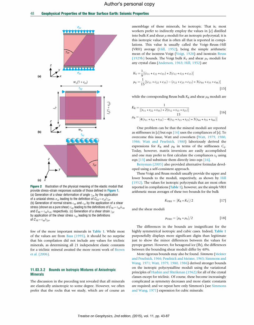
vice versa are illustrated in Figure 2. Hearmon (1946) gave
the geometry for a number of such static measurements that
could be used to fill [c].
For anisotropic materials, the configuration of [c] depends
on the material’s degree of symmetry. Such symmetry is classi-
fied within the six crystal systems listed in terms of diminishing
symmetry: cubic (or isometric), hexagonal, tetragonal, ortho-
rhombic, monoclinic, and triclinic. The literature is not neces-
sarily consistent on how many crystal systems there are, and
many authors divide the hexagonal system into separate hex-
agonal and trigonal systems for a total of 7. This classification
is used here following Auld (1990) and Tinder (2007). Regard-
less of the preference, nine different sets of stiffnesses [c] can be
defined. This is larger than the seven classes because two
unique sets exist in both the trigonal and the tetragonal sys-
tems depending on the slightly different symmetries. The lower
the symmetry, the greater the number of independent elastic
stiffnesses required. The organization of the nine different sets
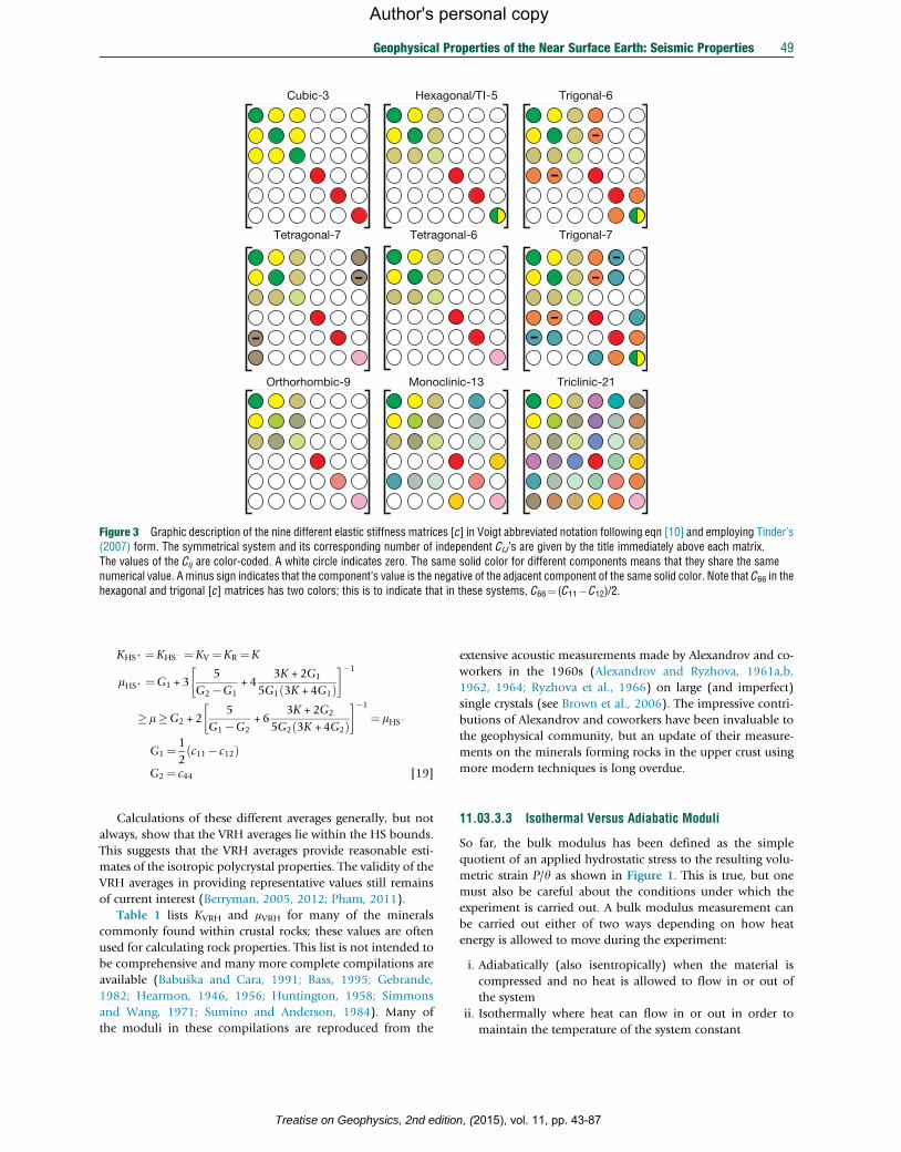
of [c] is shown symbolically in Figure 3.
Bass (1995) had compiled an extensive collection of Cij for
many minerals up to 1995, and Angel et al. (2009) provided an
overview of the techniques used to obtain these elastic con-
stants. The full sets of the values in [c] are repeated here for a
n, (2015), vol. 11, pp. 43-87
szz
szz
wo
wo(1 + exx)
I o(1
+e z
z)
(a)
(b)
(c)
x
x
x
y
y
y
z
z
z
txy
txy
g zx
gyz
l o
Figure 2 Illustration of the physical meaning of the elastic moduli thatprovide stress–strain responses outside of those defined in Figure 1.(a) Generation of a shear deformation of angle gzx by the applicationof a uniaxial stress szz leading to the definition of C53¼szz/gzx.(b) Generation of normal strains Exx and Ezz by the application of a shearstress (shown as a pure shear) txy leading to the definitions of C16¼txy/Exxand C36¼txy/Ezz, respectively. (c) Generation of a shear strain gyzby application of the shear stress txy leading to the definitionsof C16¼txy/gyz.
48 Geophysical Properties of the Near Surface Earth: Seismic Properties
Author's personal copy
few of the more important minerals in Table 1. While most
of the values are from Bass (1995), it should be no surprise
that his compilation did not include any values for triclinic
minerals, as determining all 21 independent elastic constants
for a triclinic mineral awaited the more recent work of Brown
et al. (2006).
11.03.3.2 Bounds on Isotropic Mixtures of AnisotropicMinerals
The discussion in the preceding text revealed that all minerals
are elastically anisotropic to some degree. However, we often
prefer that the rocks that we study, which are of course an
Treatise on Geophysics, 2nd edition,
assemblage of these minerals, be isotropic. That is, most
workers prefer to indirectly employ the values in [c] distilled
into bulk K and shear mmoduli for an isotropic polycrystal; it is
this isotropic value that is often all that is reported in compi-
lations. This value is usually called the Voigt–Reuss–Hill
(VRH) average (Hill, 1952), being the simple arithmetic
mean of the isostress Voigt (Voigt, 1928) and isostrain Reuss
(1929b) bounds. The Voigt bulk KV and shear mV moduli for
any crystal class (Anderson, 1963; Hill, 1952) are
KV ¼ 1
9c11 + c22 + c33ð Þ+2 c12 + c23 + c13ð Þ½ �
mV ¼1
15c11 + c22 + c33ð Þ� c12 + c23 + c13ð Þ +3 c44 + c55 + c66ð Þ½ �
[15]
while the corresponding Reuss bulk KR and shear mR moduli are
KR ¼ 1
s11 + s22 + s33ð Þ +2 s12 + s13 + s23ð Þ½ �mR ¼
15
4 s11 + s22 + s33ð Þ�4 s12 + s13 + s23ð Þ +3 s44 + s55 + s66ð Þ½ �[16]
One problem can be that the mineral moduli are reported
as stiffnesses in [c] but eqn [16] uses the compliances of [s]. To
overcome this issue, Watt and coworkers (Watt, 1979, 1980,
1986; Watt and Peselnick, 1980) laboriously derived the
expressions for KR and mR in terms of the stiffnesses Cij.
Today, however, matrix inversions are easily accomplished
and one may prefer to first calculate the compliances sij using
eqn [13] and substitute them directly into eqn [16].
Berryman (2005) also provided alternative formulas devel-
oped using a self-consistent approach.
These Voigt and Reuss moduli usually provide the upper and
lower bounds to the moduli, respectively, as shown by Hill
(1952). The values for isotropic polycrystals that are most often
reported in compilations (Table 1), however, are the simple VRH
arithmetic mean averages of these two bounds for the bulk
KVRH ¼ KR +KV½ �=2 [17]
and the shear moduli
mVRH ¼ mR +mV½ �=2 [18]
The differences in the bounds are insignificant for the
highly symmetrical isotropic and cubic cases. Indeed, Table 1
purposefully displays more significant digits than legitimate
just to show the minor differences between the values for
pyrope garnet. However, for hexagonal ice (Ih), the differences
between the bounding shear moduli differ by 40%.
More rigorous bounds may also be found. Simmons (Meister
and Peselnick, 1966; Peselnick andMeister, 1965; Simmons and
Wang, 1971; Watt, 1979, 1980, 1986) derived stronger bounds
on the isotropic polycrystalline moduli using the variational
principles of Hashin and Shtrikman (1962) for all of the crystal
classes except for triclinic. Of course, these become increasingly
complicated as symmetry decreases and more elastic constants
are required; and we repeat here only Simmon’s (see Simmons
and Wang, 1971) expression for cubic minerals:
(2015), vol. 11, pp. 43-87
Tetragonal-6
Cubic-3
Orthorhombic-9 Monoclinic-13
Hexagonal/TI-5
-
-
Trigonal-6
Tetragonal-7
-
-
-
-
Trigonal-7
Triclinic-21
-
-
Figure 3 Graphic description of the nine different elastic stiffness matrices [c] in Voigt abbreviated notation following eqn [10] and employing Tinder’s(2007) form. The symmetrical system and its corresponding number of independent CIJ’s are given by the title immediately above each matrix.The values of the Cij are color-coded. A white circle indicates zero. The same solid color for different components means that they share the samenumerical value. A minus sign indicates that the component’s value is the negative of the adjacent component of the same solid color. Note that C66 in thehexagonal and trigonal [c] matrices has two colors; this is to indicate that in these systems, C66¼ (C11�C12)/2.
Geophysical Properties of the Near Surface Earth: Seismic Properties 49
Author's personal copy
KHS+ ¼KHS� ¼KV ¼KR ¼K
mHS+ ¼G1 + 35
G2�G1+ 4
3K +2G1
5G1 3K +4G1ð Þ� ��1
� m�G2 + 25
G1�G2+ 6
3K + 2G2
5G2 3K +4G2ð Þ� ��1
¼ mHS�
G1 ¼ 1
2c11� c12ð Þ
G2 ¼ c44 [19]
Calculations of these different averages generally, but not
always, show that the VRH averages lie within the HS bounds.
This suggests that the VRH averages provide reasonable esti-
mates of the isotropic polycrystal properties. The validity of the
VRH averages in providing representative values still remains
of current interest (Berryman, 2005, 2012; Pham, 2011).
Table 1 lists KVRH and mVRH for many of the minerals
commonly found within crustal rocks; these values are often
used for calculating rock properties. This list is not intended to
be comprehensive and many more complete compilations are
available (Babuska and Cara, 1991; Bass, 1995; Gebrande,
1982; Hearmon, 1946, 1956; Huntington, 1958; Simmons
and Wang, 1971; Sumino and Anderson, 1984). Many of
the moduli in these compilations are reproduced from the
Treatise on Geophysics, 2nd editio
extensive acoustic measurements made by Alexandrov and co-
workers in the 1960s (Alexandrov and Ryzhova, 1961a,b,
1962, 1964; Ryzhova et al., 1966) on large (and imperfect)
single crystals (see Brown et al., 2006). The impressive contri-
butions of Alexandrov and coworkers have been invaluable to
the geophysical community, but an update of their measure-
ments on the minerals forming rocks in the upper crust using
more modern techniques is long overdue.
11.03.3.3 Isothermal Versus Adiabatic Moduli
So far, the bulk modulus has been defined as the simple
quotient of an applied hydrostatic stress to the resulting volu-
metric strain P/y as shown in Figure 1. This is true, but one
must also be careful about the conditions under which the
experiment is carried out. A bulk modulus measurement can
be carried out either of two ways depending on how heat
energy is allowed to move during the experiment:
i. Adiabatically (also isentropically) when the material is
compressed and no heat is allowed to flow in or out of
the system
ii. Isothermally where heat can flow in or out in order to
maintain the temperature of the system constant
n, (2015), vol. 11, pp. 43-87

Table 1 Values of the elastic stiffnesses for select materials displaying varying degrees of symmetry
Isot
rop
ic F
used
SIO
2
'ij' Cub
icP
yrop
e
hexa
gona
l ice
(Ih)
(257
K)
Trig
onal
- 6
α-q
uart
z
Trig
onal
- 7
Dol
omite
Tetr
agon
al -
6R
utile
Tetr
agon
al -
7W
ulfe
nite
Orh
torh
omb
icE
nsta
tite
Mon
oclin
icM
usco
vite
Tric
linic
Low
Alb
ite
Stiffnesses in GPa
11 78.08 296.2 13.5 86.6 205 269 109 225 183 69.9
22 78.08 296.2 13.5 86.6 205 269 109 178 178 183.5
33 78.08 296.2 14.9 106.1 113 480 92 214 59.1 179.5
44 31.38 91.6 3.09 57.8 39.8 124 26.7 77.6 16 24.9
55 31.38 91.6 3.09 57.8 39.8 124 26.7 75.9 17.6 26.8
66 31.38 91.6 3.5 40 67 192 33.7 81.6 72.4 33.5
12 15.32 111.1 6.5 6.7 71 177 68 72.4 48.3 34
13 15.32 111.1 5.9 12.6 57.4 146 53 54.1 23.8 30.8
23 15.32 111.1 5.9 12.6 57.4 146 53 52.7 21.7 5.5
14 0 0 0 −17.8 −19.5 0 0 0 0 5.1
15 0 0 0 0 13.7 0 0 0 −2 −2.4
16 0 0 0 0 0 0 −13.6 0 0 −0.9
24 0 0 0 17.8 19.5 0 0 0 0 −3.9
25 0 0 0 0 −13.7 0 0 0 3.9 −7.7
26 0 0 0 0 0 0 13.6 0 0 −5.8
34 0 0 0 0 0 0 0 0 0 −8.7
35 0 0 0 0 0 0 0 0 1.2 7.1
36 0 0 0 0 13.7 0 0 0 0 −9.8
45 0 0 0 0 0 0 0 0 0 −2.4
46 0 0 0 0 0 0 0 0 0.5 −7.2
56 0 0 0 −17.8 −19.5 0 0 0 0 0.5
KV
36.24 172.8
8.722 38.1 99.4 217 73.11 108 67.5 63.8
KR 8.717 37.6 89.1 209 71.58 107 48.7 55.2
KH 8.72 37.85 94.25 213 72.35 108 58.1 59.50
mV
31.38
91.98 3.5093 47.6 51.8 124.6 19.75 76.2 43 41.2
mR 91.98 5.689 41 40 98.7 25.33 75.2 27.6 29.8
mH 92.0 4.60 44.3 45.9 111.7 22.5 75.7 35.3 35.5
MV
78.08
295.4 13.4 101.6 168.5 383.1 99.44 210 125 118.7
MR 295.4 13.3 92.2 142.4 340 105.4 208 85.4 94.93
MH 295.4 13.4 96.9 155.5 361.6 102.4 209 105 106.8
Cell color fills correlate to the symbolic representation of the Voigt elastic stiffness matrices in Figure 3. Values are taken from Bass (1995) except for isotropic fused SiO2(Ohno et al., 2000) and triclinic low albite (Brown et al., 2006). Values in bold are calculated from the other elastic stiffnesses.
50 Geophysical Properties of the Near Surface Earth: Seismic Properties
Author's personal copy
A propagating compressional wave consists of alternating
zones of high pressure and low pressure that are slightly hotter
and colder, respectively, than the initial ambient temperature.
An isothermal state could only be achieved if during a half-
period, the heat could fully conduct from the high- to the low-
pressure regions. This is in fact difficult to achieve (Condon,
1933; Fletcher, 1974, 1976) with the somewhat paradoxical
result that isothermal conditions can only be reached at
Treatise on Geophysics, 2nd edition,
extremely high frequencies where, in a gas, the wavelengths
are comparable to the mean free path of the molecules
(Condon, 1933).
Table 2 is typical of the types of data presented in the
literature for such properties but its simplicity does hide a
number of complications that the reader, usually simply look-
ing for a value to use, should still keep in mind. The first is that
the values reported are usually the VRH averages as just noted.
(2015), vol. 11, pp. 43-87

Geophysical Properties of the Near Surface Earth: Seismic Properties 51
Author's personal copy
The values reported are also usually the adiabatic bulk moduli
as would be measured using acoustic techniques.
In most of the solid crystalline materials, this will insignif-
icantly differ from the isothermal bulk modulus KT obtained
from static measurements carried out at constant temperature.
Voigt (1928) (p. 788; see also Hearmon (1946)) provided the
relationship between the isothermal ikT and the adiabatic sij
compliances:
sTik ¼ sik +aiakTrCP
[20]
where r is the density, T is the absolute temperature in �K, CP is
the heat capacity at constant pressure, and ai is the appropriatecomponent of the thermal expansion tensor (see Landau and
Lifshitz, 1970, Section 10). This difference can often be ignored
for most minerals, although for KCl, the two S12 values differ
by 18%. The reader may be able to obtain appropriate values
for ai and CP and formulas for their correction to pressure and
temperature in the compilations of Holland and Powell
(1998). It is important to note, however, that these differences
cannot generally so easily be ignored for fluids. This issue will
be discussed in more detail later.
11.03.3.4 Effects of Pressure and Temperature on MineralModuli
The values in Table 2 are for the most part provided under
standard or room conditions. In many cases, in the upper crust,
the use of such values as ‘constants’ is generally valid as the
variations with pressure and temperature will be small. For
example, the variations in the properties are usually ignored
in petroleum and near-surface seismology. Those studying
shallow and high-temperature geothermal systems may, how-
ever, need to take such variations into account.
Even though we can often ignore their effects, the moduli for
various minerals are not constants and do depend on both the
temperature and the confining pressure. With increasing confin-
ing pressure, minerals become stiffer and more rigid, and the
first-order derivatives of the bulk dK/dP and dm/dP are positive
and the range for most minerals is between 4–6 Pa Pa�1 and
0.5–2 Pa Pa�1, respectively. Conversely, the moduli decrease
Table 2 Density, isotropic bulk moduli, and isotropic polycrystalline wav
Material Density (kg m�3)Adiabatic bulkmodulus K (GPa)
Tectosilicatesa-Quartz 2648 37.8b-Quartza 2522 42.97Albite 2610b 56.9Anorthite 2765b 84.2Orthoclase 2571b 62Microcline 2567 55.4NeosilicatesForsterite 3221 129.5Fayalite 4380 134Fo91Fa9 3325 129.5Grossular 3602 168.4Pyrope 3567 172.8Inosilicates
Treatise on Geophysics, 2nd editio
with temperature with dK/dT��5 MPa �K�1 to�30 MPa �K�1.
As such, within the crust, temperature will usually influence the
moduli more than pressure. The changes in the moduli and
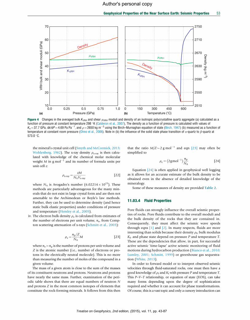
density of an isotropic polycrystalline quartz compact with pres-
sure and temperature are shown for purposes of illustration in
Figure 4. These suggest that the effects of pressure and temper-
ature tend to cancel each other out, although in areas with steep
thermal gradients, the changes in temperature can significantly
alter the bulk modulus and the density of the quartz. The range
of temperatures is intentionally shown to reflect the larger var-
iations in the physical properties of the quartz in the vicinity of
the a-quartz to b-quartz phase transition.
11.03.3.5 Mineral Densities
Equations [1] and [2] also include the material’s bulk density
r. Consider a rock composed of m separate mineral phases
each with density ri and fi of the fractional volume of the
material (with Sfi¼1). The density for this rock takes the form
r¼Xmi¼1
firi [21]
Our knowledge of mineral density is often taken for
granted, but in reality, it may not always be so easy to deter-
mine and a number of different methods are applied. While
usually the differences are small, one may still need to take care
to know how the number is derived. The methods used to
determine density include the following:
i. Archimedean fluid displacement in which the mineral
sample’s volume is found from the amount of reference
fluid volume that it displaces. The density so determined is
referred to as the specific gravity and it is simply equal to
the ratio of the sample’s measured mass to the volume of
the fluid displaced.
ii. Boyle’s law pyncnometry where the sample volume is
determined by in a measurement of the deviation of the
gas pressure in a container of a known volume (Lowell
et al., 2004). The noble gas helium is usually used.
iii. x-Ray and neutron scattering crystallography that provide
information on the dimensions and hence volume Vx-ray of
e speeds
Shear modulusm (GPa)
Poisson’sratio n VP (m s�1) VS (m s�1)
44.3 0.079 6048 409041.41 0.135 6239 405228.6 0.285 6034 331039.9 0.295 7049 379929.3 0.296 6270 337628.1 0.283 6015 3309
81.1 0.241 8589 501850.7 0.332 6784 340277.6 0.250 8370 4831108.9 0.234 9331 549892 0.274 9101 5079
(Continued)
n, (2015), vol. 11, pp. 43-87

Table 2 (Continued)
Material Density (kg m�3)Adiabatic bulkmodulus K (GPa)
Shear modulusm (GPa)
Poisson’sratio n VP (m s�1) VS (m s�1)
Hornblende 3150 93.3 49.3 0.275 7105 3956Augite 3320 95 59 0.243 7233 4216Ferrosilite 4002 101 52 0.280 6524 3605Enstatite 3272 107.8 75.7 0.215 7987 4810PhyllosilicatesMuscovite (Illite?c) 2844 58.2 35.3 0.248 6084 3523Biotite 3050 50.5d 27.4d 0.270 5342 2997Kaolinite 2669b 71.1e 31.2e 0.309 6498 3419Na montmorillonite, dry 2700f 82g 32g 0.327 6795 3443Na montmorillonite, wet 1700f 36g 16.5g 0.301 5841 3115Talch 2793 41.6 22.6 0.270 5068 2845Lizarditei 2516 61 33.9 0.265 6400 3600Antigoritej 2668 69 34.0 0.288 6520 3570EvaporitesCalcite 2712 73.3 32 0.309 6539 3435Aragonite 2930 46.9 38.5 0.178 5790 3625Dolomite 3795 94.9 45.7 0.293 6408 3470Anhydrite 2963 54.9 29.3 0.273 5631 3145Gypsum 2317 42 15.4 0.337 5195 2578Halite 2163 24.9 14.7 0.253 4536 2607Sylvite 1987 18.1 9.4 0.279 3926 2175Barite 4473 55 22.8 0.318 4369 2258OxidesCorundum 3982 253.5 163.2 0.235 10877 6402Magnetite 5206 161 91.4 0.261 7371 4190Periclase 3584 160 130.3 0.180 9650 6030Ice-I (270 K) 917.5 8.73 3.4 0.328 3802 1925SulfidesPyrite 5016 142.7 125.7 0.160 7865 5006Galena 7597 58.6 31.9 0.270 3649 2049Sphalerite 4088 77.1 31.5 0.320 5398 2776OthersDiamond 3512 443 535.7 0.069 18153 12350Graphite 2260 161.0 109.3 0.223 11650 6954FluidsAir (STP) dryk 1.31 0.00014311 – – 330.2 –Water (STP)l 999.84 1.97 – – 1402.4 –Seawater (STP), 35% salinitym 1032.8 2.17 – – 1449.1 –Light oil (1 atm, 26 �C)n 750 1.15 – – 1237 –Heavy oil (1 atm, 26 �C)n 1037 2.71 – – 1616 –Tholeiitic basalt 1505 �Ko 2650 17.9 – – 2599 –Andesite melt 1553 �Ko 2440 16.1 – – 2569 –Rhyolite melt 1553 �Ko 2310 13.5 – – 2417 –
Unless otherwise indicated, the densities, adiabatic bulk moduli, and shear moduli are all from Bass (1995). The seismic velocities are calculated using eqns [1] and [2].aFrom Table 4 of Ohno et al. (2006) at 575.5 �C.bDensities from Smyth and McCormick (1995).cSee discussion in Cholach and Schmitt (2006).dValue is the Voigt–Reuss–Hill average calculated assuming hexagonal symmetry (Watt and Peselni, 1980) using the values reported in Bass (1995).eValue is the Voigt–Reuss–Hill average calculated assuming hexagonal symmetry (Watt and Peselni, 1980) using the values reported in Karmous (2011). See also Militzer et al. (2011)
and Sato et al. (2005).fDensities of a dry and saturated montmorillonite as updated by Chitale and Sigal (2000).gValue is the Voigt–Reuss–Hill average calculated assuming hexagonal symmetry (Watt and Peselni, 1980) using the elastic stiffness calculated in Ebrahimi et al. (2012).hDensity and estimates of moduli in Bailey and Holloway (2000).iEstimates from Auzende et al. (2006). See also Schmitt et al. (2007).jFrom measurements described in Christensen (2004). See also recent modeling by Mookherjee and Stixrude (2009).kFrom Lemmon et al. (2000).lOnline calculation Lemmon et al. (2012a) derived from the model of Wagner and Pruss (2002).mFrom Wong and Zhu (1995) and Safarov et al. (2012).nFrom ultrasonic measurements of Wang et al. (1990).oZero frequency (relaxed) estimates based on ultrasonic measurement of Rivers and Carmichael (1987) as reported in Bass (1995).
52 Geophysical Properties of the Near Surface Earth: Seismic Properties
Treatise on Geophysics, 2nd edition, (2015), vol. 11, pp. 43-87
Author's personal copy
0.0 0.25 0.5 0.75 1.010
20
30
40
50
60
70
2510
2550
2590
2630
2670
2710
2750
0 150 300 450 600
KVRHKVRH
VR
H b
ulk
and
she
ar m
odul
i (G
Pa)
Density (kg m
−3)
Temperature (�C)
Density
Density
mVRHmVRH
(a) (b)Pressure (GPa)
Figure 4 Changes in the averaged bulk KVRH and shear mVRH moduli and density of an isotropic polycrystalline quartz aggregate (a) calculated as afunction of pressure at constant temperature 298 �K (Calderon et al., 2007), The density as a function of pressure is calculated with values ofKo¼37.7 GPa, dk/dP¼4.69 Pa Pa�1, and r¼2650 kg m�3 using the Birch–Murnaghan equation of state (Birch, 1947) (b) measured as a function oftemperature at constant room pressure (Ohno et al., 2006). Note in (b) the influence of the solid state phase transition of a-quartz to b-quartz at573.0 �C.
Geophysical Properties of the Near Surface Earth: Seismic Properties 53
Author's personal copy
the mineral’s crystal unit cell (Smyth and McCormick, 2013;
Wohlenberg, 1982). The x-ray density rx-ray is then calcu-
lated with knowledge of the chemical molar molecular
weight M in g mol�1 and its number of formula units per
unit cell z:
rx-ray ¼zM
NAVx-ray[22]
where NA is Avogadro’s number (6.02214�1023). These
methods are particularly advantageous for the many min-
erals that do not exist in large crystal form and are then not
amenable to the Archimedean or Boyle’s law methods.
Further, they can be used to determine density (and hence
static bulk elastic properties) under conditions of pressure
and temperature (Hemley et al., 2005).
iv. The electron bulk density re is calculated from estimates of
the number of electrons per unit volume, ne, from Comp-
ton scattering attenuation of x-rays (Schmitt et al., 2003):
re ¼np=Z
NAM [23]
where ne¼np is the number of protons per unit volume and
Z is the atomic number (i.e., number of electrons or pro-
tons in the electrically neutral molecule). This is no more
than measuring the number of moles of the compound in a
given volume.
The mass of a given atom is close to the sum of the masses
of its constituent neutrons and protons. Neutrons and protons
have nearly the same mass. Further, examination of the peri-
odic table shows that there are equal numbers of neutron N
and protons Z in the most common isotopes of elements that
constitute the rock-forming minerals. It follows from this then
Treatise on Geophysics, 2nd editio
that the ratio M/Z�2 g mol�1 and eqn [23] may often be
simplified to
re ¼ 2gmol�1� � np
NA[24]
Equation [24] is often applied in geophysical well logging
as it allows for an accurate estimate of the bulk density to be
obtained even in the absence of detailed knowledge of the
mineralogy.
Some of these measures of density are provided Table 2.
11.03.4 Fluid Properties
Pore fluids can strongly influence the overall seismic proper-
ties of rocks. Pore fluids contribute to the overall moduli and
the bulk density of the rocks that they are contained in.
Consequently, they must affect the seismic wave speeds
through eqns [1] and [2]. In many respects, fluids are more
interesting than solids because their density rf, bulk modulus
Kf, and phase state depend on pressure P and temperature T.
These are the dependencies that allow, in part, for successful
active seismic ‘time-lapse’ active seismic monitoring of fluid
motions during hydrocarbon production (Bianco et al., 2010;
Lumley, 2001; Schmitt, 1999) or greenhouse gas sequestra-
tion (White, 2013).
In order to forward model or to interpret observed seismic
velocities through fluid-saturated rocks, one must then have a
good knowledge of rf and Kf with pressure P and temperature T.
This P–V–T relationship, or equation of state (EOS), can take
many forms depending upon the degree of sophistication
required and whether it can account for phase transformations.
Of course, this is a vast topic and only a cursory introduction can
n, (2015), vol. 11, pp. 43-87
54 Geophysical Properties of the Near Surface Earth: Seismic Properties
Author's personal copy
be given here with particular focus on some key fluids that
researchers would encounter including water, carbon dioxide,
and methane. While as geophysicists we would prefer to be
handed easily obtained values for the desired properties, this
may not always be possible and some work may be required to
obtain appropriate representative values. The reader should not
necessarily look for quick answers here, but this contribution
attempts to at least lead the way to the relevant literature where
answers might be found. An important contribution of Batzle
and Wang (1992), for example, has distilled some of these
complex relations into more readily applicable formulas. Their
equations have been incorporated into numerous fluid property
calculators for use in seismic fluid substitution calculations;
because they are so widely used, these too will be provided
where appropriate. This section attempts to give some appreci-
ation of how complicated and interesting fluid properties are,
particularly relative to the more consistent minerals.
11.03.4.1 Phase Relations for Fluids
Before proceeding further, it is important to review the pressure
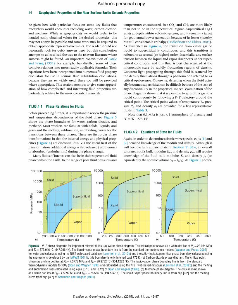
and temperature dependencies of the fluid phase. Figure 5
shows the phase boundaries for water, carbon dioxide, and
methane. Most workers are familiar with solids, liquids, and
gases and the melting, sublimation, and boiling curves for the
transitions between these phases. These are first-order phase
transformations in that the internal energy and physical prop-
erties (Figure 6) are discontinuous. Via the latent heat of the
transformation, additional energy is also released (exothermic)
or absorbed (endothermic) during the phase change.
Many fluids of interest can also be in their supercritical fluid
phase within the Earth. In the range of pore fluid pressures and
Temperature (K) Temp400 500 600 700 800 900
Ice VII
Ice VII
Solid
Liquid
Vapor
Supercritical
0.1
1
10
100
1000
10 000
200
Solid
Liquid
250 3000.1
1
10
100
1000
10 000
100 000
Pre
ssur
e (M
Pa)
200 300
Ice
1Ic
e III
Ice
V Ic
e VI
(a) (b)
Figure 5 P–T phase diagrams for important relevant fluids. (a) Water phaseand TC¼373.946 �C (647.096 �K). The liquid–vapor phase boundary line is ffor water and calculated using the NIST web-based database (Lemmon et al., 2the expressions developed by the IAPWS (2011); this boundary is only inferrshown as a white dot lies at PC¼7.3773 MPa and TC¼30.9782 �C (304.1282thermodynamic models for CO2 (Span and Wagner, 1996) and calculated usinand sublimation lines calculated using eqns [3.10] and [3.12] of Span and Was a white dot lies at PC¼4.5992 MPa and TC¼�78.586 �C (194.564 �K). Tcurve from eqn [3.7] of Setzmann and Wagner (1991).
Treatise on Geophysics, 2nd edition,
temperatures encountered, free CO2 and CH4 are more likely
than not to be in the supercritical regime. Supercritical H2O
exists at depth within volcanic systems, and it remains a target
for geothermal power generation because of its lower viscosity
but still considerable enthalpy (Fridleifsson and Elders, 2005).
As illustrated in Figure 6, the transition from either gas or
liquid to supercritical is continuous, and this transition is
referred to as second (or higher)-order. Essentially, any surface
tension between the liquid and vapor disappears under super-
critical conditions, and this fluid is best characterized at the
microscopic scale by rapidly fluctuating regions of density.
Coherent light propagating through this fluid is scattered by
the density fluctuations through a phenomenon referred to as
critical opalescence. Otherwise, detecting when the fluid actu-
ally becomes supercritical can be difficult because of the lack of
any discontinuity in the properties. Indeed, examination of the
phase diagrams shows that it is possible to go from a gas to a
liquid continuously by following a P–T trajectory around the
critical point. The critical point values of temperature Tc, pres-
sure Pc, and density rc are provided for a few representative
fluids in Table 3.
Note that 0.1 MPa is just <1 atmosphere of pressure and�C¼�K�273.15�.
11.03.4.2 Equations of State for Fluids
Again, in order to determine seismic wave speeds, eqns [1] and
[2] demand knowledge of the moduli and density. Although it
will become fully apparent later in Section 11.03.6, an overall
saturated rock’s bulk modulus Ksat and density rsat will requireknowledge of the fluid bulk modulus Kf and density rf (orequivalently the specific volume Vf¼1/rf). As Figure 6 shows,
erature (K) Temperature (K)350 400 450 500
Supercritical
0.1
1
10
100
1000
10 000
50 150
Solid
Vapor
250 350 450 550
Supercritical
Vapor
Liquid
(c)
diagram: The critical point shown as a white dot lies at PC¼22.064 MParom the standard thermodynamic models (Wagner and Pruss, 2002)012b) and the solid–liquid/supercritical phase boundary calculated usinged past 775 K. (b) Carbon dioxide phase diagram: The critical point�K). The liquid–vapor phase boundary line is from the standardg the NIST web-based database (Lemmon et al., 2012b) and the meltingagner (1996). (c) Methane phase diagram: The critical point shownhe liquid–vapor phase boundary line is from eqn [3.2] and the melting
(2015), vol. 11, pp. 43-87
0200
400
600
800
1000
Pressure (MPa)
Pressure (MPa)
Press
ure (
MPa)
Pressure (MPa)
Density (kg
m-3)
0100
200
300
400
500
0.00
5
0.03
0.05
5
0.08
0.10
5
1015202530
Enthalpy (kJm
ol –1)
Tem
perat
ure (
C)
Tempera
ture (C
)
Temperature (C)
Temperature (C
)
Viscosity cP
Bulk m
odulus (M
Pa)
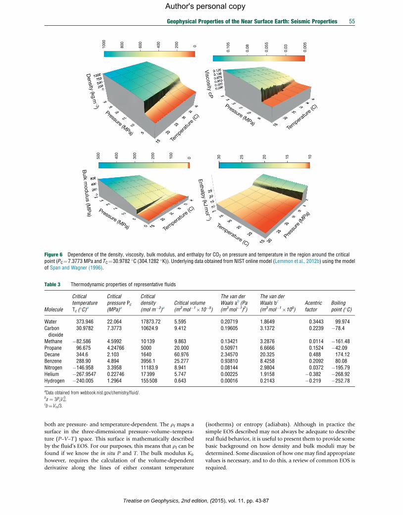
Figure 6 Dependence of the density, viscosity, bulk modulus, and enthalpy for CO2 on pressure and temperature in the region around the criticalpoint (PC¼7.3773 MPa and TC¼30.9782 �C (304.1282 �K)). Underlying data obtained from NIST online model (Lemmon et al., 2012b) using the modelof Span and Wagner (1996).
Table 3 Thermodynamic properties of representative fluids
Molecule
CriticaltemperatureTc (�C)a
Criticalpressure Pc(MPa)a
Criticaldensity(mol m�3)a
Critical volume(m3mol�1�10�5)
The van derWaals ab (Pa(m3mol�1)2)
The van derWaals bc
(m3mol�1�105)Acentricfactor
Boilingpoint (�C)
Water 373.946 22.064 17873.72 5.595 0.20719 1.8649 0.3443 99.974Carbondioxide
30.9782 7.3773 10624.9 9.412 0.19605 3.1372 0.2239 �78.4
Methane �82.586 4.5992 10139 9.863 0.13421 3.2876 0.0114 �161.48Propane 96.675 4.24766 5000 20.000 0.50971 6.6666 0.1524 �42.09Decane 344.6 2.103 1640 60.976 2.34570 20.325 0.488 174.12Benzene 288.90 4.894 3956.1 25.277 0.93810 8.4258 0.2092 80.08Nitrogen �146.958 3.3958 11183.9 8.941 0.08144 2.9804 0.0372 �195.79Helium �267.9547 0.22746 17399 5.747 0.00225 1.9158 �0.382 �268.92Hydrogen �240.005 1.2964 155508 0.643 0.00016 0.2143 �0.219 �252.78
aData obtained from webbook.nist.gov/chemistry/fluid/.ba ¼ 3PcVm
3.cb¼Vm/3.
Geophysical Properties of the Near Surface Earth: Seismic Properties 55
Author's personal copy
both are pressure- and temperature-dependent. The rf maps a
surface in the three-dimensional pressure–volume–tempera-
ture (P–V–T ) space. This surface is mathematically described
by the fluid’s EOS. For our purposes, this means that rf can be
found if we know the in situ P and T. The bulk modulus Kf,
however, requires the calculation of the volume-dependent
derivative along the lines of either constant temperature
Treatise on Geophysics, 2nd editio
(isotherms) or entropy (adiabats). Although in practice the
simple EOS described may not always be adequate to describe
real fluid behavior, it is useful to present them to provide some
basic background on how density and bulk moduli may be
determined. Some discussion of how onemay find appropriate
values is necessary, and to do this, a review of common EOS is
required.
n, (2015), vol. 11, pp. 43-87
56 Geophysical Properties of the Near Surface Earth: Seismic Properties
Author's personal copy
11.03.4.2.1 Ideal gas lawThe simplest EOS is that for a perfect gas that considers the gas
molecules to be point masses of no volume such that
PVm ¼RT [25]
where R¼8.3144621(7575) J mol�1�K�1 is the gas constant,
Vm is the molar volume in m3mol�1, and T is the temperature
in degrees kelvin. Note that rf¼1/Vf¼M/Vm. The P–Vm rela-
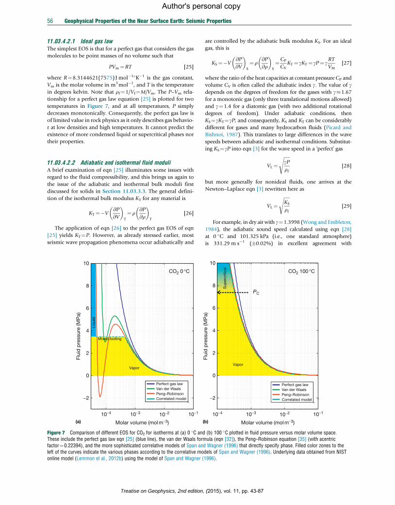
tionship for a perfect gas law equation [25] is plotted for two
temperatures in Figure 7, and at all temperatures, P simply
decreases monotonically. Consequently, the perfect gas law is
of limited value in rock physics as it only describes gas behavio-
r at low densities and high temperatures. It cannot predict the
existence of more condensed liquid or supercritical phases nor
their properties.
11.03.4.2.2 Adiabatic and isothermal fluid moduliA brief examination of eqn [25] illuminates some issues with
regard to the fluid compressibility, and this brings us again to
the issue of the adiabatic and isothermal bulk moduli first
discussed for solids in Section 11.03.3.3. The general defini-
tion of the isothermal bulk modulus KT for any material is
KT ¼�V@P
@V
� �T
¼ r@P
@r
� �T
[26]
The application of eqn [26] to the perfect gas EOS of eqn
[25] yields KT¼P. However, as already stressed earlier, most
seismic wave propagation phenomena occur adiabatically and
10-4 10-3 10-2 10-1
−2
0
2
4
6
8
10
Molar volume (mol m-3)
Flui
d p
ress
ure
(MP
a)
Perfect gas law
Peng–RobinsonCorrelated model
Liq
uid
Vapor
CO2 0 °C
Mixed-boiling
(a) (
Van der Waals
Figure 7 Comparison of different EOS for CO2 for isotherms at (a) 0 �C andThese include the perfect gas law eqn [25] (blue line), the van der Waals formfactor¼0.22394), and the more sophisticated correlative models of Span andleft of the curves indicate the various phases according to the correlative moonline model (Lemmon et al., 2012b) using the model of Span and Wagner (
Treatise on Geophysics, 2nd edition,
are controlled by the adiabatic bulk modulus KS. For an ideal
gas, this is
KS ¼�V@P
@V
� �S
¼ r@P
@r
� �S
¼CP
CVKT ¼ gKT ¼ gP¼ g
RT
VM[27]
where the ratio of the heat capacities at constant pressure CP and
volume CV is often called the adiabatic index g. The value of gdepends on the degrees of freedom for the gases with g�1.67
for a monotonic gas (only three translational motions allowed)
and g¼1.4 for a diatomic gas (with two additional rotational
degrees of freedom). Under adiabatic conditions, then
KS¼gKT¼gP; and consequently, KS and KT can be considerably
different for gases and many hydrocarbon fluids (Picard and
Bishnoi, 1987). This translates to large differences in the wave
speeds between adiabatic and isothermal conditions. Substitut-
ing KS¼gP into eqn [3] for the wave speed in a ‘perfect’ gas
VL ¼ffiffiffiffiffigPrf
s[28]
but more generally for nonideal fluids, one arrives at the
Newton–Laplace eqn [3] rewritten here as
VL ¼ffiffiffiffiffiKS
rf
s[29]
For example, in dry air with g¼1.3998 (Wong and Embleton,
1984), the adiabatic sound speed calculated using eqn [28]
at 0 �C and 101.325 kPa (i.e., one standard atmosphere)
is 331.29 m s�1 (0.02%) in excellent agreement with
10-4 10-3 10-2 10-1
Molar volume (mol m-3)
Flui
d p
ress
ure
(MP
a)
Sup
ercr
itica
l
Vapor
CO2 100 °C
0
2
4
6
8
10
-2
PC
b)
Perfect gas law
Peng–RobinsonCorrelated model
Van der Waals
(b) 100 �C plotted in fluid pressure versus molar volume space.ula (eqn [32]), the Peng–Robinson equation [35] (with acentricWagner (1996) that directly specify phase. Filled color zones to the
dels of Span and Wagner (1996). Underlying data obtained from NIST1996).
(2015), vol. 11, pp. 43-87

Geophysical Properties of the Near Surface Earth: Seismic Properties 57
Author's personal copy
experimental observations. In contrast, the isothermal sound
speed first predicted by Newton would be only �280 m s�1.
As will be apparent later, an appropriate value for the fluid
bulk modulus Kf is necessary to calculate the saturated rock
properties. In the following discussions, we will assume that
the fluid bulk modulus Kf that needs to be found is the adia-
batic, or isentropic, bulk modulus KS. It is worth mentioning
that VL as defined by eqn [29] is at low frequencies with the
system at equilibrium a thermodynamic property in its own
right; in the fluid physics and engineering communities, VL is
called the thermodynamic sound speed (Castier, 2011; Picard
and Bishnoi, 1987).
Similarly to eqn [20], adiabatic and isothermal bulk moduli
are related through
1
KS¼ 1
KT� a2TrCP
[30]
where a is the coefficient of thermal expansion, T is the tem-
perature in K, r is the density, and CP is the isobaric (i.e.,
constant pressure) heat capacity (Clark, 1992; Kieffer, 1977).
11.03.4.2.3 The van der Waals modelThe deficiencies of the perfect gas law of equation [25] were
recognized early. In order to attempt to resolve these problems,
van der Waals (1873) adapted eqn [25] by assigning the mol-
ecules a finite molar volume b and allowing them minor self-
attractive ‘van der Waals’ forces to develop his EOS
P + a=V2m
� �Vm�bð Þ¼RT [31]
that may alternatively be displayed in its polynomial
cubic form
V3m� b+
RTcPc
� �V2m +
a
PcVm�ab
Pc¼ 0 [32]
Factor a describes the weak self-attraction of the gas mole-
cules to one another, and a is proportional to the liquid’s
vaporization energy. Factor b is roughly equivalent to the
molar volume of the liquid. These constants may be found
from the fluid’s Tc and Pc:
a¼ RTcð Þ264Pc
b¼RTc8Pc
[33]
The reader will note in Figure 7 that the isotherm of the van
der Waals curve at 0 �C (i.e., below the critical temperature Tcwhere two phases can exist at a given pressure) displays cubic
behavior with three possible real roots. The smallest and largest
solutions provide the molar volumes of the liquid and the
vapor, respectively, while the intermediate root has no real
physical meaning. At sufficiently high temperatures or at low
pressures, only one real root exists. While not obvious to the
more casual reader, this shape allows for the prediction of
liquid, gas, and supercritical regimes. The real fluid does not
follow the trajectory in the region of the function’s trough and
peak, which is actually a mixed-phase region where the liquid
and vapor coexist until either condensation or boiling is com-
plete. Castellan (1971) contains a particularly clear discussion
of the information that may be obtained from the van der
Treatise on Geophysics, 2nd editio
Waals curves that are beyond the scope of the discussion
here. Carcione et al. (2006) had applied the van der Waals
formula to obtain appropriate fluid moduli and density for use
in modeling of the seismic behavior of CO2 saturated rocks.
11.03.4.2.4 The Peng–Robinson EOSThe development of the van der Waals equation [31] was a
major improvement over the perfect gas law equation [25], but
as examination of Figure 7(a) shows, it is not at all accurate in
the fluid state; and a plethora of additional formulas have been
developed to overcome this to varying degrees of complication.
The Peng and Robinson (1976) modification to the van der
Waals formula
P +aPRaPR
V2m + 2bPRVm�b2PR
� �Vm�bPRð Þ¼RT [34]
remains one of the most popular in that it retains much of the
simplicity of the van der Waals EOS but provides better esti-
mates of the P–V–T relations. In eqn [34], there are three
factors that are obtained from tabulated values that include
the Peng–Robinson aPR and bPR
aPR ¼ 0:45724RTcð Þ2Pc
bPR ¼ 0:07780RTc8Pc
[35]
and the acentric factor o that accounts for nonsphericity of the
molecule (Bett et al., 2003). The effects of the acentricity and
temperature are included in aPR:
aPR ¼ 1+ 0:37464+ 1:5422o�0:26992o2� �
1�ffiffiffiffiffiffiffiffiffiffiT=Tc
p h i2[36]
The cubic form of the Peng–Robinson equation [34] is
most often for simplicity given in terms of the compressibility
factor Z¼PVm/RT with
Z3� 1�Bð ÞZ2 + A�3B2�2B� �
Z� AB�B2�B3� �¼ 0 [37]
where
A¼ aPRP
RTð Þ2
B¼ bPRP
RT
[38]
and, as for the van der Waals equation, in the two-phase region
below Tc, the largest and smallest roots correspond to the vapor
and liquid molar volumes, respectively.
The Peng–Robinson equation [34] predicts well the P–V–T
relationship for in the vapor and supercritical regimes. The
liquid properties are not as precise but depending on
the application may be sufficient. In Figure 7, for example,
the Peng–Robinson EOS value for Vm at the boiling point
exceeds that observed by about 7%. It too shows cubic behav-
ior below Tc and the same arguments used for the van der
Waals equation [32] hold. The Peng–Robinson equation [34]
was a seminal development, and a very large literature of
adaptations and additional corrections to it has emerged. It is
particularly heavily used in the petroleum industry to describe
P–V–T relations of both in situ and produced hydrocarbons.
n, (2015), vol. 11, pp. 43-87

58 Geophysical Properties of the Near Surface Earth: Seismic Properties
Author's personal copy
11.03.4.2.5 Correlative EOS modelsThe best models, at least for monomolecular fluids, are those
constructed by fitting of actual observed experimental measure-
ments. As such, these correlative models rely on the existence of
solid experimental observations of P–V–T relations and phase
boundaries and of course can only be as good as the quality of
the data and are limited by the ranges of conditions over which
measurements have been made (Setzmann and Wagner, 1989).
Models exist for important geophysical fluids including water
(Wagner and Pruss, 2002), CO2 (Span and Wagner, 1996; see
also Han et al. (2010, 2011)), and methane (Kunz and Wagner,
2012; Setzmann andWagner, 1991). The formulas used in these
models are extensive and are not repeated here as they are
lengthy and dependent on the phase state. The correlative
model for CO2 is shown as the ‘reference’ against which the
other simpler models are compared in Figure 7. Online calcu-
lation of isotherms (P–V–T paths of constant temperature), iso-
bars (P–V–T paths of constant pressure), and isochors (P–V–T
paths of constant volume or density) is available from Lemmon
et al. (2012b) for a number of important fluids. Independent
software for water properties may also be found for water (NIST,
2010b) and for other fluids and mixtures of interest to geophys-
ics (NIST, 2010a).
Pure water has been extensively studied and numerous less
complicated expressions exist with validity over more limited
Treatise on Geophysics, 2nd edition,
ranges of P and T and a large literature exists. A few of the
contributions in this area for liquid water in include those of
Del Grosso and Mader (1972) and Kell (1975).
Batzle and Wang (1992) provided a number of simplified
equations for the acoustic properties of water based on earlier
experimental work of many authors (Helgeson and Kirkham,
1974; Rowe and Chou, 1970; Wilson, 1959). For example,
based on Rowe and Chou’s (1970) compilation, they derived
a formula for the density of pure water rw (in g cm�3) as a
function of pressure P (in MPa) and temperature T (in �C)
rw ¼ 1 +10�6 �80T�3:3T2 + 0:00175T3 + 489P�2TPð
+ 0:016T2P�1:3�10�5T3P�0:333P2�0:002TP2Þ [39]
and provided Wilson’s (1959) empirical regression for the
speed of sound Vw (longitudinal wave in m s�1) in pure water
Vw ¼ 1 P P2 P3� � w00 w10 w20 w30 w40
w01 w11 w21 w31 w41
w02 w12 w22 w32 w42
w03 w13 w23 w33 w43
2664
3775
1TT2
T3
T4
266664
377775 [40]
with the coefficients wij
w00 w10 w20 w30 w40
w01 w11 w21 w31 w41
w02 w12 w22 w32 w42
w03 w13 w23 w33 w43
2666664
3777775¼
1402:85 4:871 �0:04783 1:487�10�4 �2:197�10�7
1:524 �0:0111 2:747�10�4 �6:503�10�7 7:987�10�10
3:437�10�3 1:739�10�4 �2:135�10�6 �1:455�10�8 5:230�10�11
�1:197�10�5 �1:628�10�6 1:237�10�8 1:327�10�10 �4:614�10�13
2666664
3777775 [41]
2.2
2.3
2.4
Adia
batic
Isotherm
BW
dul
us (G
Pa)
Wilson’s equation [40] may be adequate for fluid substitution
use under field conditions (Chen and Millero, 1976), whereas
in the laboratory, the more recent correlation models
(Lemmon et al., 2012a; Wagner and Pruss, 2002) or more
recent formulas (Belogol’skii et al., 1999; Lin and Trusler,
2012; Vance and Brown, 2010) may be preferable if greater
accuracy is desired. That said, the adiabatic bulk modulus
predicted using eqns [39] and [40] from Batzle and Wang
(1992) agrees well with other models (Figure 8).
1.9
2.0
2.1
0 20 40 60 80 100
al
Bul
k m
o
Temperature (�C)
Figure 8 Comparison of the bulk moduli of liquid water at 1atmosphere from 0 to 100 �C for (i) isothermal KT (blue line) calculatedusing expressions in Kell (1975), the adiabatic KS (green line) ascalculated from the correlative model sound speeds and densities fromLemmon et al. (2012b), and a second adiabatic KS (red line) calculatedfrom the Batzle and Wang (1992) formulas for density (eqn [40]) andsound speed (eqn [41]). Note that the peak in the bulk moduli arises fromthe unique behavior of water.
11.03.4.2.6 Determining Kf from equations of stateIdeally, the best way to obtain the adiabatic fluid bulkmodulus
Kf is from direct determinations of the sound speed and density
in the fluid subject to the appropriate P–T conditions (Clark,
1992; Picard and Bishnoi, 1987). Equations [26] and [27]
provide the definitions of the isothermal KT and adiabatic KS
bulk moduli as the partial derivative of P with Vm. In principle
then, one may simply obtain KT or KS by appropriately
differentiating, respectively, either an isotherm (such as
shown in Figure 7) or a corresponding adiabat. This is done
relatively easily for the isotherms for which we can write
explicit equations as in the preceding text, and, ignoring imper-
fections in the EOS itself, KT can then be easily obtained.
Unfortunately, for purposes of seismic wave propagation, KS
is the one required as discussed in Section 11.03.3.3. From the
EOS, KS can be determined in different ways:
(2015), vol. 11, pp. 43-87

Geophysical Properties of the Near Surface Earth: Seismic Properties 59
Author's personal copy
i. Assuming that the differences are small such that KS�KT.
This may be true in some cases, but even for liquid water at
1 atmosphere, the two deviate above 20 �C (Figure 8). This
assumption becomes even more problematic for hydrocar-
bon fluids. In practical interpretation of seismic data, the
errors in determining seismic velocities may be greater than
the differences produced by using KT, but workers should
still take care when assuming KT is sufficient.
ii. Obtaining KT by derivation of the isotherm and then apply-
ing eqn [30] assuming appropriate knowledge of CP and a.One problem with this approach is that the knowledge of
these parameters may be incomplete or erroneous.
iii. Numerically converting the P–V isotherms to P–V isentropes
and taking the derivative of these directly (Picard and
Bishnoi, 1987). Again, this approach can be fraught with
additional error. Clark (1992) noted that this may be the
only way to obtain a value for KS particularly for complex
multiphase fluids but it should be recognized that the EOSs
are usually imperfect (as demonstrated in Figure 7). She
recommended that, if possible, workers should find KS by
measuring the sound speeds in the fluids directly with eqn
[29]. Plantier et al. (2008) also echoed this caveat on the
direct application of thermodynamic relations to predict
wave speeds or bulk moduli in heavy oils.
An alternative strategy to calculate the isentropic compress-
ibility and hence the fluid’s thermodynamic sound speed has
recently been developed by Nichita et al. (2010). They obtain-
ed the relevant parameters from partial derivatives of the total
enthalpy with respect to temperature at constant pressure and
composition.
11.03.4.3 Mixtures and Solutions
The discussion in the preceding text focuses primarily on sim-
ple fluids with a single chemical component, but in the Earth,
this will rarely be the case. Pore waters are never pure and
usually contain numerous solvated ions and absorbed gases
(van Weert and van der Gun, 2012). Hydrocarbon-saturated
rocks actually contain a complex mixture of different organic
species mixed both miscibly and immiscibly, with water and
free gas often residing separately from the oil in the same pore.
Perhaps most importantly, the pore space can hold the fluid in
pockets of liquids and gas, a mixture with unexpected mechan-
ical properties (the so-called ‘patchy’ saturation). Conse-
quently, we must look at the topic of fluid mixtures from a
number of different perspectives as solutions, mixtures of
immiscible fluids, and mixed phases.
11.03.4.3.1 Frozen mixtures‘Frozen’ fluid mixtures can consist of either (i) a mix of immis-
cible and nonchemically interacting fluids or (ii) a mix of
vapor and liquid phases of the same fluid, the proportions of
which do not vary during passage of the seismic wave. In his
classic text, Wood (1955) developed the formula for the wave
speed in a bubbly fluid with liquid and gas phases in pro-
portions of fl and fg, respectively, and of bulk moduli Kl
and Kg, respectively (Wilson, 2005),
Treatise on Geophysics, 2nd editio
Vf ¼ffiffiffiffiffiffiffiffiffiffiffiffiffiffiffiffiffiffiffiffiffiffiffiffiffiffiffiffiffiffiffiffiffiffiffiffiffiffiffiffiffiffiffiffiffiffiffiffiffiffiffiffiffiffiffiffiffiffiffiffiffiffi
1
flrl +fgrg
fl=Kl +fg=Kg
vuut [42]
where he assumed no chemical interaction between the phases
and that the Laplace surface tension pressure in the gas bubbles
was negligible (i.e., the bubbles were sufficiently large
approximately >0.1 mm in water). By analogy to eqn [29],
the bulk modulus is
Kf ¼ fl=Kl +fg=Kg
�1[43]
In the rock physics literature, eqn [43] has been extended to
mixtures of n fluids and further generalized to include sus-
pended solids within the liquid. It is often assumed to be an
exact representation:
Kf ¼Xni¼1
fi=Ki
!�1
[44]
For purposes of illustration and following Wood’s example,
consider a mixture of air and water. The density of the mixture
increases linearly from that for air to that for water but its bulk
modulus remains much closer to that for air and only rises to
that for water in at near 100% water content (Figure 9(a)).
Conversely, a few bubbles within the water have a large influ-
ence on diminishing the mixture’s bulk modulus. This leads to
the unexpected result that the wave speed in the mixture is
substantially less than that in either air or water (Figure 9(b)),
a consequence of the competition between stiffness and den-
sity in eqn [3].
As noted, the results of Figure 9 obtained using Wood’s
equation [42] are presumed to be valid at low frequencies, but
the formula is applied nearly universally in the geophysical
literature. Nichita et al. (2010) had recently questioned even
this assumption. In reality, the physics of the problem is quite
complex with numerous additional considerations needing to
be accounted for including changes to the bulk modulus of the
gas due to Laplace internal pressure in the bubbles (e.g.,
Kieffer, 1977; Landau and Lifshitz, 1959) and of dispersion
due to a wide variety of thermal and mechanical factors (Carey
and Evans, 2011), the literature of which is too large to
review here.
One of the more popular models that considers wave speed
dispersion is that of Commander and Prosperetti (1989). This
model includes the bubble size and corresponding resonance
frequency, thermal diffusivity, and the Laplace bubble pres-
sure. Because of these factors, this model is able to determine
both mixture wave speed and attenuation with frequency. This
model, too, has another unexpected result that, while Wood’s
equation [42] appears to predict the velocities well for this case
below a few hundred Hz, above the resonance frequency for
the bubbles, the stiffness of the mixture increases dramatically
with surprisingly unexpected wave speeds above 15000 m s�1
(Figure 10). Cheyne et al. (1995) provided a heuristic descrip-
tion of this phenomenon. The minimum near 3 kHz is at the
bubble resonance frequency; and the subresonant (‘Wood’s
regime’) and superresonant regimes will shift left and right as
the mean bubble dimensions increase and decrease, respec-
tively. The point of showing these phenomena is not so
n, (2015), vol. 11, pp. 43-87
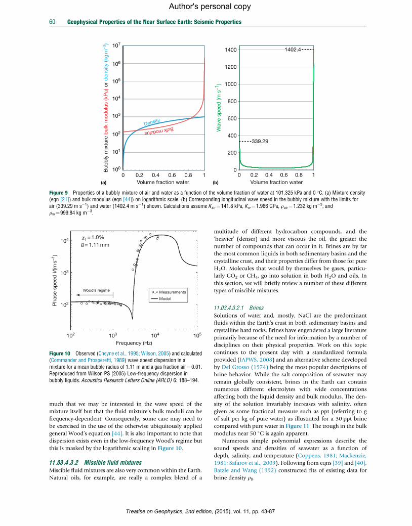
107
106
105
104
103
102
101
100Bub
bly
mix
ture
bul
k m
odul
us (k
Pa)
or
den
sity
(kg
m-3
)
Density
Bulkmodulus
0
200
400
600
800
1000
1200
1400
Wav
e sp
eed
(m s-1
)
339.29
1402.4
Volume fraction water Volume fraction water0 0.2 0.4 0.6 0.8 1 0 0.2 0.4 0.6 0.8 1
(a) (b)
Figure 9 Properties of a bubbly mixture of air and water as a function of the volume fraction of water at 101.325 kPa and 0 �C. (a) Mixture density(eqn [21]) and bulk modulus (eqn [44]) on logarithmic scale. (b) Corresponding longitudinal wave speed in the bubbly mixture with the limits forair (339.29 m s�1) and water (1402.4 m s�1) shown. Calculations assume Kair¼141.8 kPa, Kw¼1.966 GPa, rair¼1.232 kg m�3, andrw¼999.84 kg m�3.
Frequency (Hz)
Wood’s regime Measurements
Model
Pha
se s
pee
d V
(ms−1
)
102
102
103
103
104
104
105
c1= 1.0%a = 1.11 mm
Figure 10 Observed (Cheyne et al., 1995; Wilson, 2005) and calculated(Commander and Prosperetti, 1989) wave speed dispersion in amixture for a mean bubble radius of 1.11 m and a gas fraction air¼0.01.Reproduced from Wilson PS (2005) Low-frequency dispersion inbubbly liquids. Acoustics Research Letters Online (ARLO) 6: 188–194.
60 Geophysical Properties of the Near Surface Earth: Seismic Properties
Author's personal copy
much that we may be interested in the wave speed of the
mixture itself but that the fluid mixture’s bulk moduli can be
frequency-dependent. Consequently, some care may need to
be exercised in the use of the otherwise ubiquitously applied
general Wood’s equation [44]. It is also important to note that
dispersion exists even in the low-frequency Wood’s regime but
this is masked by the logarithmic scaling in Figure 10.
11.03.4.3.2 Miscible fluid mixturesMiscible fluid mixtures are also very common within the Earth.
Natural oils, for example, are really a complex blend of a
Treatise on Geophysics, 2nd edition,
multitude of different hydrocarbon compounds, and the
‘heavier’ (denser) and more viscous the oil, the greater the
number of compounds that can occur in it. Brines are by far
the most common liquids in both sedimentary basins and the
crystalline crust, and their properties differ from those for pure
H2O. Molecules that would by themselves be gases, particu-
larly CO2 or CH4, go into solution in both H2O and oils. In
this section, we will briefly review a number of these different
types of miscible mixtures.
11.03.4.3.2.1 Brines
Solutions of water and, mostly, NaCl are the predominant
fluids within the Earth’s crust in both sedimentary basins and
crystalline hard rocks. Brines have engendered a large literature
primarily because of the need for information by a number of
disciplines on their physical properties. Work on this topic
continues to the present day with a standardized formula
provided (IAPWS, 2008) and an alternative scheme developed
by Del Grosso (1974) being the most popular descriptions of
brine behavior. While the salt composition of seawater may
remain globally consistent, brines in the Earth can contain
numerous different electrolytes with wide concentrations
affecting both the liquid density and bulk modulus. The den-
sity of the solution invariably increases with salinity, often
given as some fractional measure such as ppt (referring to g
of salt per kg of pure water) as illustrated for a 30 ppt brine
compared with pure water in Figure 11. The trough in the bulk
modulus near 50 �C is again apparent.
Numerous simple polynomial expressions describe the
sound speeds and densities of seawater as a function of
depth, salinity, and temperature (Coppens, 1981; Mackenzie,
1981; Safarov et al., 2009). Following from eqns [39] and [40],
Batzle and Wang (1992) constructed fits of existing data for
brine density rB
(2015), vol. 11, pp. 43-87
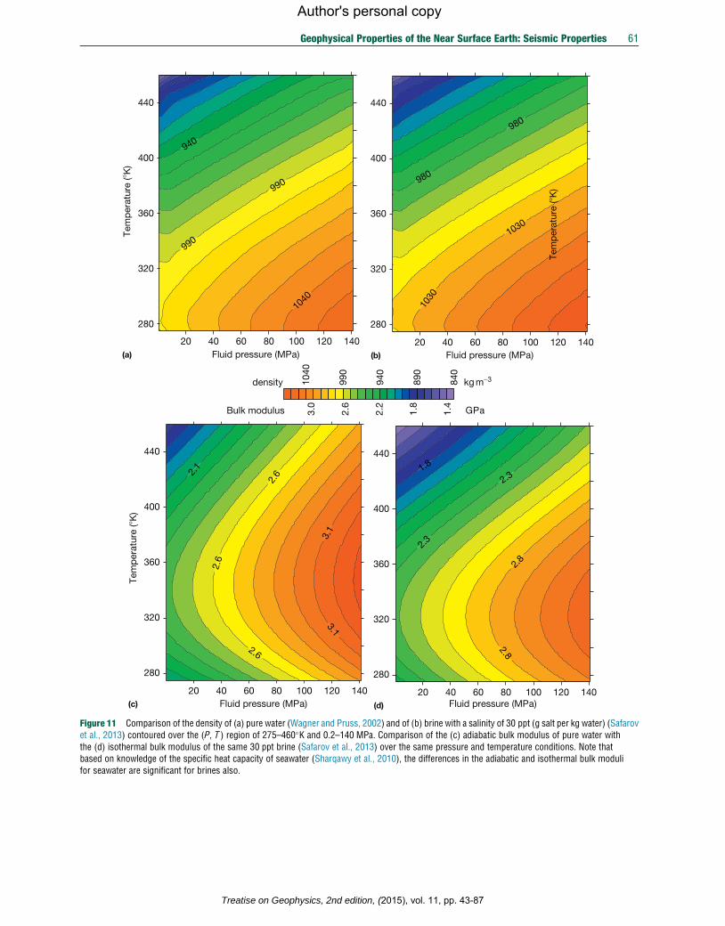
20 40
1030
1030
980
980
60 80 100 120 140
280
320
360
400
440
840
890
940
990
1040
1.4
1.8
2.2
2.6
3.0
20(a) (b)
(c) (d)
40 60 80 100 120 140
1040
990
990
940
280
320
360
400
440
Tem
per
atur
e (�
K)
Tem
per
atur
e (�
K)
Tem
per
atur
e (�
K)
20 40 60 80 100 120 14020 40 60 80 100 120 140
280
320
360
400
440
280
320
360
400
440
Bulk modulus
density kg m−3
GPa
Fluid pressure (MPa) Fluid pressure (MPa)
Fluid pressure (MPa)Fluid pressure (MPa)
2.1
2.6
2.6
3.1
3.1
2.6
1.8
2.3
2.3
2.8
2.8
Figure 11 Comparison of the density of (a) pure water (Wagner and Pruss, 2002) and of (b) brine with a salinity of 30 ppt (g salt per kg water) (Safarovet al., 2013) contoured over the (P, T ) region of 275–460�K and 0.2–140 MPa. Comparison of the (c) adiabatic bulk modulus of pure water withthe (d) isothermal bulk modulus of the same 30 ppt brine (Safarov et al., 2013) over the same pressure and temperature conditions. Note thatbased on knowledge of the specific heat capacity of seawater (Sharqawy et al., 2010), the differences in the adiabatic and isothermal bulk modulifor seawater are significant for brines also.
Geophysical Properties of the Near Surface Earth: Seismic Properties 61
Treatise on Geophysics, 2nd edition, (2015), vol. 11, pp. 43-87
Author's personal copy

Bubble
poin
t line
100%
Liqu
id
Dew point line
80%
60%
40%
20%
Cricod
entherm
Pure
fluid
A
Pure fluid B
C
Vapor
Liquid
Supercritical
Temperature
Pre
ssur
e
Pre
ssur
e (p
sia)
Temperature (�F)
M
N
O
P
(a)
(b)
Cricodenbar
1400
1200
1000
800
600
400
200
00 100 200 300 400 500
A2A3
A1
C1
C2
C3
C7A
B1 B2B3B
C
Bubblepoint line
Dewpo
int lin
e
n-Hep
tane
Etha
ne
No. wt% EthaneC 100.00C1 90.22C2 50.25C3 9.78C7 n-Heptane
Composition
Figure 12 (a) Illustration of the phase boundaries for a 50–50multicomponent mixture of pure fluids A and B with liquid, vapor, andsupercritical regions adapted from Ezekwe (2010). The boiling lines andcritical points for the two pure fluids are shown in red and green forfluids A and B, respectively. Point C is the pseudocritical point for the
62 Geophysical Properties of the Near Surface Earth: Seismic Properties
Author's personal copy
rB ¼ rw + S1 0:668+0:44S +10�6�
� 300P�2400PS +T 80+ 3T�3300S�13P +47PSð Þ½ �Þ[45]
and sound speed VB
VB ¼Vw + S 1170�9:6T +0:055T2�8:5�10�5T3�
+2:6P�0:0029TP�0:0476P2Þ+ S1:5 780�10P +0:16P2
� ��820S2 [46]
where S is the salinity in terms of the weight fraction in ppm/
106. They noted that these were for NaCl concentrations and
could be in significant error for other electrolytes particularly
with divalent anions.
The lack of information on the properties of more concen-
trated brines is an important gap in our knowledge. The exten-
sive work of Safarov et al. (2013) only reaches 30 ppt, but in
situ natural brines can reach full salt saturations with salinities
approaching 300 ppt. Data at higher concentrations are more
difficult to find, but some appropriate density information
might be obtained to 5.5 molal (320 ppt) in Rogers and
Pitzer (1982), Gucker et al. (1975), and LaLiberte and
Cooper (2004). Formation waters in the Earth too also can
have quite different compositions than seawater, with a wide
variety of ions including the cations Na+, Ca2+, Mg2+, Fe2+, K+,
Ba2+, Li+, and Sr2+ and anions Cl�, SO42�, HCO3, CO3
2�,NO3
�, Br�, I�, and S2�. Kumar (2003) measured wave speeds
in KCl solutions but there is little in the literature on the effect
of these ions on the acoustic properties of the solution. These
few citations are in no way intended to be exhaustive, and there
are many contributions that discuss the properties of brines.
However, most of the work is performed under conditions,
particularly of pressure, that are below what is needed in situ,
and workers may need to take care in regard to the range of
applicability of a given formulation.
mixture. Percentages represent the saturation proportions of liquid togas in the mixed-phase region between the bubble and dew point lines.(b) Mixed-phase envelopes for various proportions of ethane andn-heptane. The single-component boiling lines for ethane and n-heptaneare shown in red and purple, respectively, in analogy to (a). The phasecurves for three differing mixture compositions 1, 2, and 3 are shownwith the bubble and dew point lines in blue and green and with theircorresponding pseudocritical point. The yellow line is an envelope of thecritical points and highlights the compositional dependence of themixture’s critical points. Adapted from Ezekwe N (2010) PetroleumReservoir Engineering Practice. New York: Prentice Hall; Figure 4.5.
11.03.4.3.2.2 Multicomponent fluid mixtures
Multicomponent mixtures in this section refer to miscible
combinations of different gases and liquids, that is, a single-
phase solution that is formed from two or more fluids. Car-
bonated water is one example. Natural hydrocarbon oils are
another; they are quite complex and will literally contain thou-
sands of different molecules. Indeed, we expect that such mix-
tures are likely the rule, not the exception, within the Earth.
Such mixtures have many of the same characteristics as the
pure fluids described in the preceding text, but with significant
complications.
In addition to pressure P, volume V, and temperature T, the
proportions xi of the different fluids in the mixture and their
respective solubilities must also now be considered. As such,
the literature on the study of the behavior of such mixtures is
immense and the field remains an active area of research.
Consider a mixture of two fluids A and B. The phase dia-
gram of this multicomponent system in Figure 12 is broadly
similar to that for the single components shown in Figure 5
except for the zone in P–T space separating the pure fluid
and the vapor phases from one another. For the pure com-
pounds of Figure 5, this boundary is only a line. For a miscible
mixture in Figure 12, the boundary instead becomes an area in
P–T space in which both liquid and vapor coexist. This
Treatise on Geophysics, 2nd edition,
mixed-phase zone lies between the single-component boiling
lines of the two pure fluids A and B.
For purposes of illustration, it is useful to follow the
changes of a 50–50 mixture of two fluids along a hypothetical
pathM–N–O–P in P–T space in Figure 12. AtM, the mixture is
a homogeneous liquid. It remains a homogeneous liquid with
decreasing pressure until point N is reached. Here, the path
meets the bubble point line whereupon the first trace of vapor
phase appears. From the appearance of this first gas bubble at
N, the phase transformation progresses with varying satura-
tions (i.e., proportions of liquid to gas) as one travels from N
toO. At O, called the dew point, the last vestige of liquid phase
remains. Past the dew point O and downward in pressure to P,
the fluid is a homogenous vapor.
(2015), vol. 11, pp. 43-87
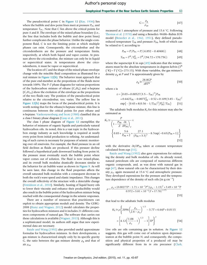
Geophysical Properties of the Near Surface Earth: Seismic Properties 63
Author's personal copy
The pseudocritical point C in Figure 12 (Kay, 1936) lies
where the bubble and dew point lines meet at pressure PPC and
temperature TPC. Note that C lies above the critical points for
pure A and B. The envelope of the mixed-phase boundary (i.e.,
the line that includes both the bubble and dew point lines)
further complicates the phase behavior. Unlike the single-com-
ponent fluid, C is not the limiting point at which multiple
phases can exist. Consequently, the cricondenbar and the
cricondentherm are the pressure and temperature limits,
respectively, at which both liquid and vapor coexist. At pres-
sure above the cricondenbar, the mixture can only be in liquid
or supercritical states. At temperatures above the crico-
ndentherm, it must be vapor or supercritical.
The location ofC and the shape of themixed-phase envelope
change with the miscible fluid composition as illustrated for a
real mixture in Figure 12(b). The behavior must approach that
of the pure end-member as the proportions of the fluids move
towards 100%. The P–T phase diagrams for various proportions
of the hydrocarbon mixture of ethane (C2H6) and n-heptane
(C7H16) show the evolution of the envelope as the proportions
of the two fluids vary. The position of the pseudocritical point
relative to the cricondenbar, too, varies. The yellow line in
Figure 12(b) maps the locus of the pseudocritical points. It is
worth noting that for the ethane/n-heptane mixture, this line is
continuous between the critical points for pure ethane and
n-heptane. Vankonynenburg and Scott (1980) classified this as
a class I binary phase diagram (Gray et al., 2011).
The class I phase diagram of Figure 12 exemplifies the
behavior of mixtures of organic liquids and particularly natural
hydrocarbon oils. As noted, this is a vast topic in the hydrocar-
bon energy industry as such knowledge is required at nearly
every point from initial production to refining. An understand-
ing of such curves is necessary for purposes of seismic monitor-
ing over oil reservoirs. For example, the fluid pressure in an oil
field declines as fluids are produced. If this pressure decline
followed a hypothetical path downward leading from point M,
the pressure must eventually reach the bubble point where
vapor comes out of solution. The fluid is now mixed-phase,
and its overall bulk modulus drastically decreases similar to
the behavior for air bubble water as shown in Figure 9. As will
be seen later, this change in the fluid properties affects the
overall saturated bulk modulus with a consequent decrease in
both the rock’s wave speed and elastic impedance. This changes
the overall reflectivity of the structure with a detectable change
(Fereidoon et al., 2010). Similarly, heating of liquid heavy oils
to lower their viscosity and enhance their producibility would
also result in the bubble point of the hydrocarbonmixture being
reached with the consequential change in the seismic responses.
There are a number of resources that practitioners can
exploit to obtain appropriate moduli and density. The GERG-
2008 (Kunz and Wagner, 2012) model calculates the proper-
ties for hydrocarbon mixtures and it includes 21 different com-
mon components of natural gas. The software that carries out
these calculations is available (Wagner, 2013). Although this is
a sophisticated model, its authors still argue that new experi-
mental data are necessary.
Batzle and Wang (1992) also provided useful approximate
formulas for hydrocarbon mixtures. In their developments, a
gas mixture is characterized simply only by its specific gravity
G, the ratio between the gas mixture density rg and that of
air rair
Treatise on Geophysics, 2nd editio
G¼ rgrair
[47]
measured at 1 atmosphere of pressure and 15.6 �C. FollowingThomas et al. (1970) and using a Benedict–Webb–Rubin EOS
model (Benedict et al., 1942, 1951), they defined pseudo-
reduced temperature TPR and pressure PPR, both of which can
be related to G according to
PPR ¼ P=PPC ¼ P= 4:892�0:4048Gð Þ [48]
TPR ¼ TK=TKPC ¼ TK= 94:72 +170:75Gð Þ [49]
where the superscript K in eqn [49] indicates that the temper-
atures must be the absolute temperatures in degrees kelvin (TK
(�K)¼T (�C)+273.15). With these variables, the gas mixture’s
density rg at P and T is approximately given by
rg ffi28:8GP
zRTK[50]
where z is
z¼ 0:03 +0:00527 3:5�TPRð Þ3� �PPR
+ 0:642TPR �0:007T4PR �0:52 + 0:109 3:85�TPRð Þ2
exp � 0:45 +8 0:56�1=TPRð Þ2� �P1:2PR =TPR
�[51]
The adiabatic bulk modulus KS for this mixture may also be
estimated as
KS ffi P
1�PPRZ
@z
@PPR
� �T
�
0:85 +5:6
PPR + 2+
27:1
PPR + 3:5ð Þ2�8:7exp �0:65 PPR + 1ð Þ½ �( )
[52]
with the derivative @z/@PPR taken at constant temperature
calculated from eqn [51].
Batzle and Wang (1992) also gave expressions for estimat-
ing the density and bulk modulus of oils. As already noted,
natural petroleum oils are composed of numerous different
organic compounds, and, as was done with natural gas in
eqn [47], these natural oils can be characterized by their den-
sity ro, again measured at 15.6 �C and atmospheric pressure.
They developed expressions for the pressure and the tempera-
ture dependence of the density of such oils (in g cm�3)
r¼ ro + 0:00277P�1:71�10�7P3ð Þ ro�1:15ð Þ2 + 3:49�10�4P
0:972 + 3:81�10�4 T + 17:78ð Þ1:175[53]
that lead to the adiabatic bulk modulus
KS ffi r 2096ro
2:6�ro
� �1=2
�3:7T +4:64P + 0:0115
(
� 4:121:08
ro�1
� �1=2
�1
" #TP
)2
[54]
Live oils are oils containing gas in solution. As Figure 12
suggests, this gas will come out of solution upon depressur-
ization at the bubble point N; and consequently, the compo-
sition and physical properties of a produced oil may be
significantly different from its in situ precursor (Clark,
n, (2015), vol. 11, pp. 43-87
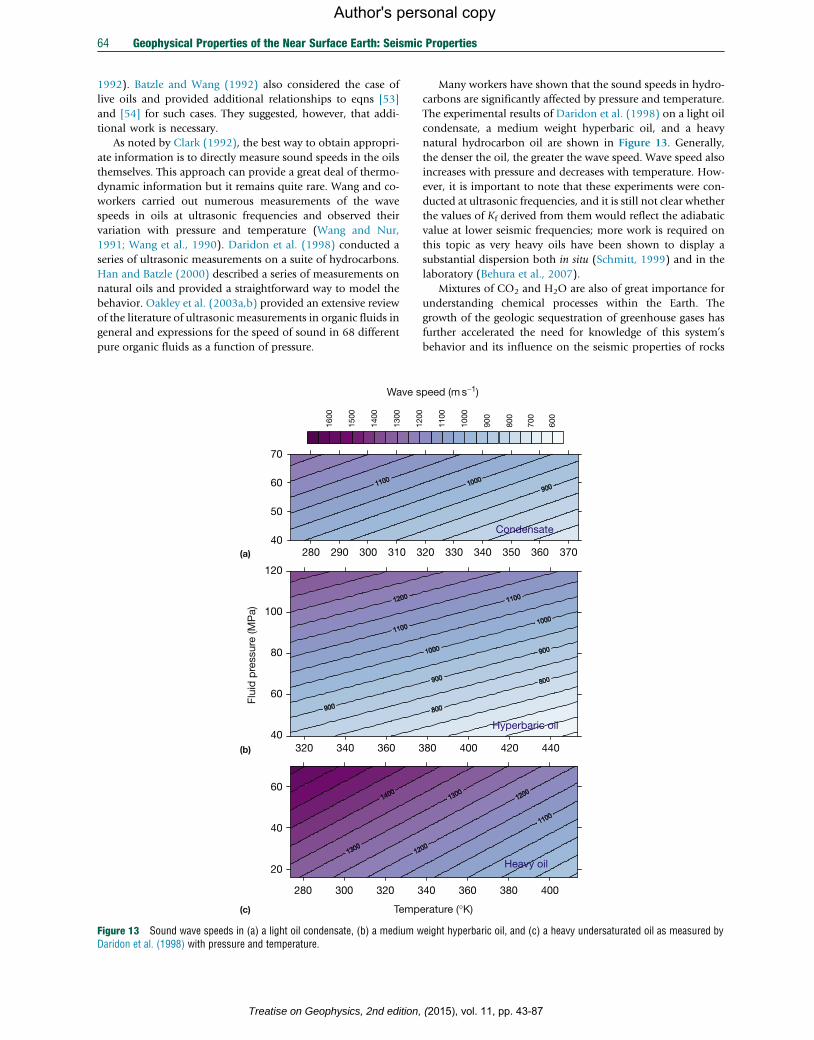
64 Geophysical Properties of the Near Surface Earth: Seismic Properties
Author's personal copy
1992). Batzle and Wang (1992) also considered the case of
live oils and provided additional relationships to eqns [53]
and [54] for such cases. They suggested, however, that addi-
tional work is necessary.
As noted by Clark (1992), the best way to obtain appropri-
ate information is to directly measure sound speeds in the oils
themselves. This approach can provide a great deal of thermo-
dynamic information but it remains quite rare. Wang and co-
workers carried out numerous measurements of the wave
speeds in oils at ultrasonic frequencies and observed their
variation with pressure and temperature (Wang and Nur,
1991; Wang et al., 1990). Daridon et al. (1998) conducted a
series of ultrasonic measurements on a suite of hydrocarbons.
Han and Batzle (2000) described a series of measurements on
natural oils and provided a straightforward way to model the
behavior. Oakley et al. (2003a,b) provided an extensive review
of the literature of ultrasonic measurements in organic fluids in
general and expressions for the speed of sound in 68 different
pure organic fluids as a function of pressure.
280 300 320 3
20
40
60
320 340 360 340
60
80
100
120
1300
1400
1500
1600
280 290 300 310 340
50
60
70
Temp
Wave s
Flui
d p
ress
ure
(MP
a)
(a)
(b)
(c)
Figure 13 Sound wave speeds in (a) a light oil condensate, (b) a medium wDaridon et al. (1998) with pressure and temperature.
Treatise on Geophysics, 2nd edition,
Many workers have shown that the sound speeds in hydro-
carbons are significantly affected by pressure and temperature.
The experimental results of Daridon et al. (1998) on a light oil
condensate, a medium weight hyperbaric oil, and a heavy
natural hydrocarbon oil are shown in Figure 13. Generally,
the denser the oil, the greater the wave speed. Wave speed also
increases with pressure and decreases with temperature. How-
ever, it is important to note that these experiments were con-
ducted at ultrasonic frequencies, and it is still not clear whether
the values of Kf derived from them would reflect the adiabatic
value at lower seismic frequencies; more work is required on
this topic as very heavy oils have been shown to display a
substantial dispersion both in situ (Schmitt, 1999) and in the
laboratory (Behura et al., 2007).
Mixtures of CO2 and H2O are also of great importance for
understanding chemical processes within the Earth. The
growth of the geologic sequestration of greenhouse gases has
further accelerated the need for knowledge of this system’s
behavior and its influence on the seismic properties of rocks
40 360 380 400
80 400 420 440
900
1000
1100
1200
600
700
800
20 330 340 350 360 370
erature (°K)
peed (m s−1)
Condensate
Hyperbaric oil
Heavy oil
eight hyperbaric oil, and (c) a heavy undersaturated oil as measured by
(2015), vol. 11, pp. 43-87
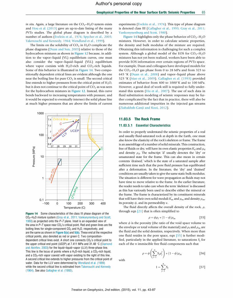
Geophysical Properties of the Near Surface Earth: Seismic Properties 65
Author's personal copy
in situ. Again, a large literature on the CO2–H2O system exists
and Hou et al. (2013) gave an up-to-date listing of the many
PVTx studies. The global phase diagram is described by a
number of authors (Evelein et al., 1976; Spycher et al., 2003;
Takenouchi and Kennedy, 1964; Wendland et al., 1999).
The limits on the solubility of CO2 in H2O complicate the
phase diagrams (Duan and Sun, 2003) relative to those of the
hydrocarbon mixtures as shown in Figure 12 because, in addi-
tion to the vapor–liquid (VL) equilibrium curves, one must
also consider the vapor–liquid–liquid (VLL) equilibrium
where vapor coexists with H2O-rich and CO2-rich liquids.
Some of this behavior is illustrated in Figure 14. Two compo-
sitionally dependent critical lines are evident although the one
near the boiling line for pure CO2 is small. The second critical
line extends to higher pressures from the critical point of H2O,
but it does not continue to the critical point of CO2 as was seen
for the hydrocarbon mixtures in Figure 12. Instead, this curve
bends backward to increasing temperatures with pressure, and
it would be expected to eventually intersect the solid phase line
at much higher pressures that are above the limits of current
0.1
1
10
100
1000
-100 100 200 300 400
6.6
6.8
7
7.2
7.4
27 28 29 30 31
LLVUCEP
C
Critical line
Critica
l line
C
Pre
ssur
e (M
Pa)
Temperature (C)0
Pure H
2O
Pur
e C
O2
Pure CO 2
Figure 14 Some characteristics of the class III phase diagram of theCO2–H2O mixture system (Gray et al., 2011; Vankonynenburg and Scott,1980) as projected onto the P–T plane. Inset is an expanded view ofthe area in P–T space near CO2’s critical point. Red and green lines are theboiling lines for single-component CO2 and H2O, respectively, andare the same as shown in Figure 5(a) and 5(b). These end at the respectivecritical points, also denoted as red or green C. Two composition-dependent critical lines exist. A short one connects CO2’s critical point tothe upper critical end point (UCEP) at 7.411 MPa and 31.48 �C (Diamondand Akinfiev, 2003) for the liquid–liquid–vapor (LLV) three-phase line.This line is the locus of points where a H2O-rich liquid, a CO2-rich liquid,and a CO2-rich vapor coexist with vapor existing to the right of this line.A second critical line extends to higher pressures from the critical point ofwater. Data for the LLV were determined by Wendland et al. (1999)while the second critical line is estimated from Takenouchi and Kennedy(1964). See also Gallagher et al. (1993).
Treatise on Geophysics, 2nd editio
experiments (Evelein et al., 1976). This type of phase diagram
is denoted class III (Gallagher et al., 1993; Gray et al., 2011;
Vankonynenburg and Scott, 1980).
Figure 14 highlights only the phase behavior of CO2–H2O
mixtures. However, in order to calculate seismic properties,
the density and bulk modulus of the mixture are required.
Obtaining this information is challenging for such a complex
system. Although a global model of the EOS for CO2–H2O
mixtures has not yet been realized, workers have been able to
provide EOS information over certain regions of PVTx space.
For example, Duan and colleagues have developed models for
the CO2–H2O gas phase from 0 to 28 MPa and from 323 to
645 �K (Duan et al., 2008) and vapor–liquid phase above
523 �K (Mao et al., 2009). Gallagher et al. (1993) provided
estimates of behavior from 400 to 1000�K and to 100 MPa.
However, a good deal of work still is required to fully under-
stand this system (Hu et al., 2007). The use of such data in
fluid substitution modeling of seismic responses may be fur-
ther complicated by the fact that in practice, there will also be
numerous additional impurities in the injected gas streams
(Ziabakhsh-Ganji and Kooi, 2012).
11.03.5 The Rock Frame
11.03.5.1 Essential Characteristics
In order to properly understand the seismic properties of a real
and usually fluid-saturated rock at depth in the Earth, one must
also know the elasticity of the rock’s skeleton or frame. The frame
is anassemblage of a number of solidminerals. This construction,
free of fluids or dry, will have its own elastic properties Kd and mdand density rd. The subscript ‘d’ usually denotes the ‘dry’ or
unsaturated state for the frame. This can also mean in certain
contexts ‘drained,’ which is the state of a saturated sample after
sufficient time such that the pore fluid pressure has equilibrated
after a deformation. In the literature, the ‘dry’ and ‘drained’
conditions are usually taken to give the same static bulkmodulus.
The situation is different for wave propagation as fluids may not
have time to move relative to the frame. In the earlier literature,
the reader needs to take care when the term ‘skeleton’ is discussed
as this has variously been used to describe either the mineral or
the frame. The frame is characterized by its constituent minerals
that will have their own solid moduli Km and mm and density rm,its porosity f, and its permeability k.
The fluid directly affects the overall density of the rock, r,through eqn [21] that is often simplified to
r¼frf + 1�fð Þrm [55]
where f is the porosity (the ratio of the void space volume to
the envelope or total volume of the material) and rf and rm are
the fluid and the solid densities, respectively. When more than
one fluid resides in the pore space, eqn [55] is further modi-
fied, particularly in the applied literature, to saturations Sj for
each of the n immiscible free fluid components such that
r¼fXnj¼1
Sjrfj
!+ 1�fð Þrm [56]
with
1¼Xnj¼1
Sj [57]
n, (2015), vol. 11, pp. 43-87

66 Geophysical Properties of the Near Surface Earth: Seismic Properties
Author's personal copy
and where rjf is the respective fluid component density.
Usually, the saturations are assigned more directly to the dif-
ferent fluid phases such as Sw, So, and Sg for water, oil, and gas,
respectively.
With these definitions out of the way, we proceed in this
section to discuss the elastic properties of the rock frame. These
frame properties are key to understanding the elasticity, and
hence the wave propagation, through rocks. Again, there is a
large literature on this topic as the study of wave propagation in
porous fluid-saturated media is important in many disciplines.
11.03.5.2 The Pore-Free Solid Portion
In this section, we are interested in the effective elastic proper-
ties of the solid frame by itself. Rocks are most commonly a
mixture of a number of minerals, and often, knowledge of the
effective bulk Km and shear mm moduli for the solid mineral
portion is a first prerequisite to the more sophisticated calcu-
lations incorporating porosity and fluids. To obtain these,
workers often assume that on average, the rock’s minerals are
randomly oriented such that the effective material is elastically
isotropic. The simplest approaches to calculating the effective
mineral moduli of the pore-free composite were derived by
Voigt (1887) and by Reuss (1929a) who, respectively, assumed
constant strain or stress within each of the components. Con-
sequently, the Voigt and Reuss formulations are mixing rules
for the stiffnesses or the compliances, respectively, such that for
N isotropic components,
KV ¼XNi¼1
fiKi �Km �XNi¼1
fi=Ki
" #�1
¼KR [58]
and
mV ¼XNi¼1
fimi � mm �XNi¼1
fi=mi
" #�1
¼ mR [59]
In eqns [58] and [59], the values of Ki and mi could be taken
from Table 2 or more extensive compilations (Bass, 1995).
Hill (1952) demonstrated that the Voigt and Reuss values
bound the composite’s effective bulk Km and shear mm moduli.
Various authors (see Watt et al. (1976)) have argued over
which of the bounds or averages provide the best values. In
practice, Hill’s simple arithmetic mean of the bounds
KVRH¼ [KR+KV]/2 and mVRH¼ [mR+mV]/2 is most usually calcu-
lated to give Km and mm as done similarly in Section 11.03.3.2
for isotropic composites of polycrystals made of a single min-
eral phase. The difference here is that the bounds are assumed
to be mixtures of isotropic materials.
Hashin and Shtrikman’s (1962) approach may also be
applied to estimating the composite’s elasticmoduli according to
K +HS ¼K1 +
f2
K2�K1ð Þ�1 +f1 K1 +4
3m1
� ��1 �Km
�K2 +f1
K1�K2ð Þ�1 +f2 K2 +4
3m2
� �¼K�HS [60]
and
Treatise on Geophysics, 2nd edition,
m +HS ¼ m1 +
f2
m2�m1ð Þ�1 +2f1 K1 + 2m1ð Þ5m1 K1 +
4
3m1
� �� mm
� m2 +f1
m1�m2ð Þ�1 +2f2 K2 + 2m2ð Þ5m2 K2 +
4
3m2
� �¼ m�HS [61]
Equations [60] and [61] are valid for only two mineral
components, but Hashin and Shtrikman (1963) also provided
the methodology to carry out the calculations for N compo-
nents (Berryman, 1995; Watt et al., 1976).
Calculations using eqns [58] through [61] are carried out
for a hypothetical mixture of quartz and calcite for purposes of
illustration in Figure 15. Such a quartz–calcite mixture is not
expected to exist naturally, but these two minerals were chosen
only because of the large differences in their elastic moduli and
because of the unusual differences between Km and mm. Equa-tion [59] gives similar values of the shear moduli with the
largest deviation between mV and mR being<3% at fquartz¼0.5.
In contrast, the Voigt and Reuss bulk moduli from eqn [58]
differ by nearly 11% at the same quartz proportion. In contrast,
the Hashin–Shtrikman bounds for both moduli of eqns [60]
and [61] differ by only a fraction of a percent. This translates
into tighter differences for the wave speeds that vary by at most
by 3.5% and 1.4% for VP and VS, respectively. Consequently,
eqns [58] through [61] are widely used to estimate Km and mmfor the rock, and there appears to be good experimental evi-
dence of their applicability to pore-free metal composites
(Hashin and Shtrikman, 1963; Umekawa and Sherby, 1966)
and to an assortment of rocks (Brace, 1965; Ji et al., 2002)
subject to high pressures.
One caveat is that in many rocks, the minerals have a
preferential crystallographic alignment due to sedimentary
deposition or metamorphic deformation. In such cases, the
minerals are no longer crystallographically randomly oriented;
and their intrinsic anisotropy affects the overall anisotropy
of the composite. These preferential mineral alignments
are variously called lattice-preferred orientations (LPO) or
crystallographic-preferred orientations (CPO) in the literature.
This requires that the various mixing theories be modified to
account for the crystal symmetries and the statistics of their
orientations with respect to that of the material.
There is insufficient room to go into details of the proce-
dures used and only a brief listing of the relevant literature is
given. Different averaging techniques were described by a vari-
ety of workers (Babuska, 1972; Bunge, 1974; Crosson and Lin,
1971; Kumazawa, 1969; Thomsen, 1972). Mainprice (1990)
provided computer programs that utilized these ideas and
applied it to a textured plagioclase rock.
Noting that the results from the Voigt and Ruess averages
are not invertible to each other (i.e., eqn [13] does not hold),
Matthies and Humbert (1993) developed the geometric mean
average that was then used by Mainprice and Humbert (1994)
on polycrystals of feldspar and biotite and by Cholach and
Schmitt (2006) to explore the effects of the strength of phyllo-
silicate orientations on the seismic anisotropy of shales and
schists. The ability to quantitatively obtain mineralogical ori-
entation distribution functions has grown greatly in the last
(2015), vol. 11, pp. 43-87
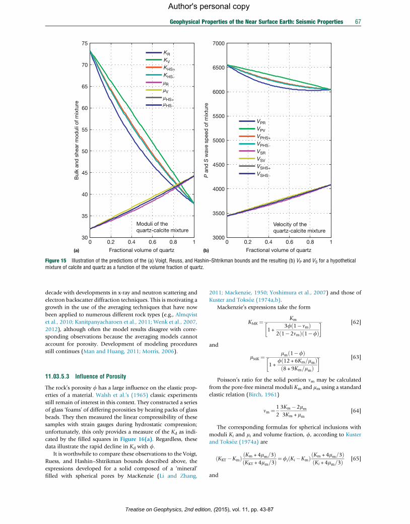
0 0.2 0.4 0.6 0.8 130
35
40
45
50
55
60
65
70
75
Bul
k an
d s
hear
mod
uli o
f mix
ture
Moduli of thequartz-calcite mixture
KR
KV
KHS+
KHS-
0 0.2 0.4 0.6 0.8 13000
3500
4000
4500
5000
5500
6000
6500
7000
P a
nd S
wav
e sp
eed
of m
ixtu
re
Velocity of thequartz-calcite mixture
VPR
VPV
VPHS+
VPHS-
VSR
VSV
VSHS+
VSHS-
mR
mV
mHS+mHS-
Fractional volume of quartz(a) (b) Fractional volume of quartz
Figure 15 Illustration of the predictions of the (a) Voigt, Reuss, and Hashin–Shtrikman bounds and the resulting (b) VP and VS for a hypotheticalmixture of calcite and quartz as a function of the volume fraction of quartz.
Geophysical Properties of the Near Surface Earth: Seismic Properties 67
Author's personal copy
decade with developments in x-ray and neutron scattering and
electron backscatter diffraction techniques. This is motivating a
growth in the use of the averaging techniques that have now
been applied to numerous different rock types (e.g., Almqvist
et al., 2010; Kanitpanyacharoen et al., 2011; Wenk et al., 2007,
2012), although often the model results disagree with corre-
sponding observations because the averaging models cannot
account for porosity. Development of modeling procedures
still continues (Man and Huang, 2011; Morris, 2006).
11.03.5.3 Influence of Porosity
The rock’s porosity f has a large influence on the elastic prop-
erties of a material. Walsh et al.’s (1965) classic experiments
still remain of interest in this context. They constructed a series
of glass ‘foams’ of differing porosities by heating packs of glass
beads. They then measured the linear compressibility of these
samples with strain gauges during hydrostatic compression;
unfortunately, this only provides a measure of the Kd as indi-
cated by the filled squares in Figure 16(a). Regardless, these
data illustrate the rapid decline in Kd with f.It is worthwhile to compare these observations to the Voigt,
Ruess, and Hashin–Shtrikman bounds described above, the
expressions developed for a solid composed of a ‘mineral’
filled with spherical pores by MacKenzie (Li and Zhang,
Treatise on Geophysics, 2nd editio
2011; Mackenzie, 1950; Yoshimura et al., 2007) and those of
Kuster and Toks€oz (1974a,b).
Mackenzie’s expressions take the form
KMK ¼ Km
1+3f 1� nmð Þ
2 1�2nmð Þ 1�fð Þ� � [62]
and
mMK ¼mm 1�fð Þ
1+f 12 +6Km=mmð Þ8 +9Km=mmð Þ
� � [63]
Poisson’s ratio for the solid portion nm may be calculated
from the pore-free mineral moduli Km and mm using a standard
elastic relation (Birch, 1961)
nm ¼ 1
2
3Km�2mm3Km +mm
[64]
The corresponding formulas for spherical inclusions with
moduli Ki and mi and volume fraction, f, according to Kuster
and Toks€oz (1974a) are
KKT�Kmð Þ Km +4mm=3ð ÞKKT + 4mm=3ð Þ¼fi Ki�Kmð Þ Km + 4mm=3ð Þ
Ki +4mm=3ð Þ [65]
and
n, (2015), vol. 11, pp. 43-87

0
10
20
30
40
50
0.4 0.6 0.8 10 0.2 0.4 0.6 0.8 10 0.2Porosity
She
ar m
odul
us (G
Pa)
WalshBerge
0
10
20
30
(a) (b)
Bul
k m
odul
us (G
Pa)
Porosity
Berge
KR and KHS–mR and mHS–
KKT & K
HS+ & K
MK
mKT & m
HS+ & m
MK
Kv
mv
Figure 16 Comparison of experimentally observed (a) bulk modulus and (b) shear modulus versus air-filled porosity in sintered porous glasscomposites from Walsh (1965) and Berge et al. (1995). Subscripts on the moduli are R, Ruess bound; V, Voigt bound; HS� and HS+,Hashin–Shtrikman bounds; KT, Kuster–Toks€oz; and MK, Mackenzie.
68 Geophysical Properties of the Near Surface Earth: Seismic Properties
Author's personal copy
mKT�mm� � mm + zmð Þ
mKT + zmð Þ¼fi mi�mmð Þ mm + zmð Þmi + zmð Þ [66]
where
zm ¼ mm 9Km + 8mmð Þ6 Km +2mmð Þ [67]
The moduli for the inclusions are taken to be zero for the
calculations shown in Figure 16. For this particular case (and
also for cases in which the spherical voids are filled with a fluid
for which mi¼0), the Reuss and the lower Hashin–Shtrikman
bounds coincide. Further, the Kuster–Toks€oz and the upper
Hashin–Shtrikman bound values also are the same, and these
are also close to those calculated using Mackenzie’s equations.
One important observation from Figure 16 is that unlike the
calculations for a nonporous mixture of solids (Figure 15), the
Voigt–Reuss bounds are less useful in predicting the moduli for
porous materials. One reason for this is the large divergence
between the vanishing moduli in the empty pore. The Hashin–
Shtrikman bounds, too, have a wide variance although the
upper bounds appear to match Walsh et al.’s (1965) bulk mod-
ulus observations reasonably well.
There is some scatter in Walsh et al.’s (1965) experimental
results in Figure 16(a), but they do trend close to but slightly
lower than the KKT�KHS+�KMK prediction line. The reason for
this most likely lies in the fact that both the Kuster–Toks€oz and
Mackenzie formulations assume ‘dilute’ amounts of spherical
voids that are sufficiently removed from one another such that
the interactions between their concentrated stress and strains
may be ignored. Interaction of the elastic fields from individual
spheres cannot be avoided once the spheres become suffi-
ciently proximate.
Numerous authors have attempted to overcome these limi-
tations by addressing such interactions by two main groups of
Treatise on Geophysics, 2nd edition,
approaches: that of an effectivematrix or that of an effective field
(Carvalho and Labuz, 1996; Mavko et al., 2003). The effective
matrix approaches are often further subdivided either into ‘self-
consistent’ methods (Budiansky and O’Connell, 1976; Hill,
1965; Wu, 1966) that consider the solids and pores as a whole
or by ‘differential effective medium’ methods in which pores are
incrementally added to a matrix in order to update its modulus,
and this revised modulus is then that of the new matrix for the
next iteration (e.g., Berryman et al., 2002; David and
Zimmerman, 2011; Kachanov, 1980; Li and Zhang, 2011;
Norris, 1985; Zimmerman, 1984). The effective field methods
developed by Mori and Tanaka (1973) place a pore in the
nonporous solid to which a stress field is then applied. The
advantage of this approach is that more complex stress fields
can be applied within the material accounting directly for the
existence of the holes. These techniques have been widely
applied in the composite materials literature but have not seen
as much application in rock physics (Sayers and Kachanov,
1995), although Kachanov et al. (1994) suggested that the
Mori–Tanaka approach may be superior. Berryman and Berge
(1996) noted the exclusivity of the use of the Mori–Tanaka
approach in the engineering literature and contrasted it with
the Kuster–Toks€oz model employed in geophysics indicating
that both are likely only valid for f<0.3. Yan et al. (2011)
gave a recent example of the use of the Mori–Tanaka approach
in estimating the frame moduli of sandstones.
The literature on modeling of rock properties using the
various developments presented earlier in the text is large and
only a small view of it is possible here. Mavko et al. (2003)
provided some starting points for further investigations.
The porosity-dependent variations in moduli transfer
through to the wave speeds according to eqns [1] and [2]. An
illustration of this effect in a suite of carbonates, primarily
clean limestones, shows the significant changes in both VP
and VS with increasing porosity. Both wave speeds decrease
(2015), vol. 11, pp. 43-87
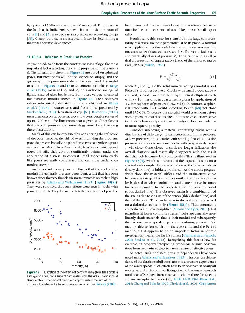
Geophysical Properties of the Near Surface Earth: Seismic Properties 69
Author's personal copy
by upward of 50% over the range of fmeasured. This is despite
the fact that the bulk density, r, which is in the denominator of
eqns [1] and [2], also decreases as f increases according to eqn
[55]. Cleary, porosity is an important factor in determining a
material’s seismic wave speeds.
11.03.5.4 Influence of Crack-Like Porosity
As just noted, aside from the constituent mineralogy, the most
important factor affecting the elastic properties of the frame is
f. The calculations shown in Figure 16 are based on spherical
pores, but most pores will not be shaped so simply; and the
geometry of the pores needs also to be considered. It is useful
to return to Figures 16 and 17 to see some of such effects. Berge
et al. (1995) measured VP and VS on sandstone analogs of
lightly sintered glass beads and, from these values, calculated
the dynamic moduli shown in Figure 16. Their observed
values substantially deviate from those obtained in Walsh
et al.’s (1965) measurements and from those predicted by
Mackenzie’s (1950) derivation of eqn [62]. Bakhorji’s (2009)
measurements on carbonates, too, show considerable scatter of
up to 1700 m s�1 for limestones near a given f. Other factors
that simplify porosity and mineralogy must be influencing
these observations.
Much of this can be explained by considering the influence
of the pore shape. At the risk of oversimplifying the problem,
pore shapes can broadly be placed into two categories: equant
or crack-like. Much like a Roman arch, large aspect ratio equant
pores are stiff; they do not significantly deform under the
application of a stress. In contrast, small aspect ratio crack-
like pores are easily compressed and can close under even
modest stresses.
An important consequence of this is that the rock elastic
moduli are generally pressure-dependent, a fact that has been
known since the very first elastic measurements on rock to high
pressures by Adams and Williamson (1923) (Figure 18(a)).
They were surprised that such effects were seen in rocks with
porosities <1%. They theoretically tested a number of possible
0 10 20 30 401000
2000
3000
4000
Dry
vel
ocity
(ms−1
)
5000
6000
7000
Porosity(%)
VpVs
Figure 17 Illustration of the effects of porosity on VP (blue filled circles)and VS (red stars) for a suite of carbonates from the Arab D formation ofSaudi Arabia. Experimental errors are approximately the size of thesymbols. Unpublished ultrasonic measurements from Bakhorji (2009).
Treatise on Geophysics, 2nd editio
hypotheses and finally inferred that this nonlinear behavior
must be due to the existence of crack-like pores of small aspect
ratio.
Heuristically, this behavior stems from the large compress-
ibility of a crack-like pore perpendicular to its plane. A normal
stress applied across the crack face pushes the surfaces towards
one another. As this stress increases, the effective crack shortens
and eventually closes at pressure Pc. For a crack with an ellip-
tical cross-section of aspect ratio w (ratio of the minor to major
axes), this is (Walsh, 1965)
Pc ¼ pEmw4 1� n2m� � [68]
where Em and nm are the solid mineral Young’s modulus and
Poisson’s ratio, respectively. Cracks with small aspect ratios ware easily closed. For example, a hypothetical elliptical crack
with w�10�3 residing in quartz matrix closes by application of
<2 atmospheres of pressure (�0.2 MPa). In contrast, a spher-
ical ‘crack’ with w¼1 would according to eqn [68] not close
until 172 GPa. Of course, the material would crush long before
such a pressure could be reached, but these calculations serve
to illustrate how easily crack-like porosity can be closed relative
to more equant porosity.
Consider subjecting a material containing cracks with a
distribution of different w’s to an increasing confining pressure.
At low pressures, those cracks with small w first close. As the
pressure continues to increase, cracks with progressively larger
w will close. Once closed, a crack no longer influences the
overall elasticity and essentially disappears with the result
that the rock becomes less compressible. This is illustrated in
Figure 18(b), which is a cartoon of the expected strains on a
cracked rock sample. As pressure increases, the observed strain
(heavy dark line) is initially nonlinear. As the cracks progres-
sively close, the material stiffens and the strain–stress curve
becomes less steep. This continues until all of the crack poros-
ity is closed at which point the strain–stress curve becomes
linear and parallel to that expected for the pore-free solid
(thick dashed line). The observed strain is a combination of
the strains due to closure of the cracks (thick dashed line) and
that of the solid. This can be seen in the real strains observed
on a dolomite rock sample (Figure 18(c)). These arguments
are perhaps a bit oversimplified (Stroisz and Fjaer, 2013), but
regardless at lower confining stresses, rocks are generally non-
linearly elastic materials, that is, their moduli and subsequently
their seismic wave speeds depend on confining pressure. One
may be able to ignore this in the deep crust and the Earth’s
mantle, but it appears to be an important factor in seismic
investigations nearer the Earth’s surface (Crampin and Peacock,
2008; Schijns et al., 2012). Recognizing this fact is key, for
example, in properly interpreting time-lapse seismic observa-
tions from reservoirs subject to varying states of effective stress.
As noted, such nonlinear pressure dependencies have been
noted since Adams andWilliamson (1923). This pressure depen-
dence of the elastic moduli translates into a pressure dependence
of the waves speeds. Such effects have been observed in nearly all
rock types and an incomplete listing of contributions where such
nonlinear effects have been observed includes those for igneous
andmetamorphic hard rocks (e.g., Birch, 1960, 1961; Blake et al.,
2013;ChengandToks€oz, 1979;Cholach et al., 2005;Christensen
n, (2015), vol. 11, pp. 43-87

70 Geophysical Properties of the Near Surface Earth: Seismic Properties
Author's personal copy
and Stanley, 2003; Goddard, 1990; Kern, 1982; Lyakhovsky et al.,
1997; Todd and Simmons, 1972), sandstones (e.g., Christensen
and Wang, 1985; Gomez et al., 2010; Jones and Nur, 1983;
Khazanehdari and McCann, 2005; Khazanehdari and Sothcott,
0
0
0
0
−1
−1
−2
−2
−3
−3
−4
−5
50
50
100
100
150
150
200
200
Hydrostatic confining stress (MPa)
Observed
Solid
Hydrostatic confining stress (MPa)
Line
ar s
trai
n (m
stra
in)
Line
ar s
trai
n (m
stra
in)
Com
pre
ssib
ility
, β X
106
Pressure in megabars(a)
(b)
(c)
0
1
2
3
4
5
2000 4000 6000 8000 10000
Crack
12000
Granites
Diorites
PeridotitesGabbros
Perpendicular
Parallel
Figure 18 Effect of cracks on the elastic properties of rocks. (a) Earlyobservations of compressibility of a series of rocks, as shown in theredrafting of Figure 7 of Adams and Williamson (1923). The gray areasrepresent the spread of the moduli they expected due to mineralogicaldifferences within a given geologically defined rock type. Note thattheir definition of a megabar¼1.0197 kg cm�2¼0.9869 atm�0.1 MPaand should not be confused with the modern Mbar¼100 GPa.(b) Illustration of the partitioning of the total observed strain intocomponents due to the cracks and the minerals as a function of pressure(redrafted from Schmitt and Li, 1995). (c) Observed strains parallel andperpendicular to the sedimentary layering in a cracked dolomite as afunction of hydrostatic confining pressure. (data from Schmittand Li, 1995).
Treatise on Geophysics, 2nd edition,
2003; Lo et al., 1986; Prasad andManghnani, 1997; Sayers, 2002;
Sayers et al., 1990; Smith et al., 2010;Wyllie et al., 1958; Xu et al.,
2006), carbonates (e.g., Alam et al., 2012; Azeemuddin et al.,
2001; Fabricius et al., 2008; Melendez Martinez and Schmitt,
2013), and mudstones (Freund, 1992; Kwon et al., 2001;
Sayers, 1999). For example, the wave speeds in a highly cracked
sandstone (Figure 19(b)) from the Cadotte formation in Alberta
vary greatly even over the relatively modest range of confining
pressures to 60 MPa (He, 2006). It is interesting to contrast this
rock’s behavior with that for a comparison brass sample that over
this pressure range has a wave speed that increases slightly due to
the pressure-dependent increase in the intrinsic crystal moduli as
described in the section on minerals in the preceding text.
Many workers have focused on different ways to describe
this nonlinearity including the use of curve fitting (Carcione
and Tinivella, 2001; Eberhart-Phillips et al., 1989; Freund,
1992; Khaksar et al., 1999; Kirstetter et al., 2006; Prasad and
Manghnani, 1997; Prikryl et al., 2005; Zimmerman, 1985),
Birch–Murnaghan equations of state (Birch, 1961), differential
2000
2500
3000
3500
4000
4500
5000
Ultr
ason
ic v
eloc
ities
(m s- 1
)
Confining pressure (MPa)
VP
Vs
(a)
(b)
VP= 5193-2147e -0.034 Peff
VS= 3046-1506e -0.0309 Peff
0 20 40 60
VP Brass
Figure 19 Example of the effects of pressure on wave speeds in acracked rock. (a) Ultrasonically determined VP (blue diamonds) and VS(red squares) as a function of hydrostatic confining pressure. VP fornonporous brass (green triangles) is shown for comparison. The fitsto eqn [70] are shown. (b) Photomicrograph (2�2 cm) undertransmitted light of the Cadotte sandstone showing its highly crackednature. Despite differences in the color of the pebbles, they are nearlypure microcrystalline quartz. Unpublished data (for sample SB009 from2457.7 m depth) and image from He (2006).
(2015), vol. 11, pp. 43-87

10-4 10-3 10-2
10-4 10-3 10-2
0
10
20
30
35
45
50
Crack porosity
Bul
k or
she
ar m
odul
us (G
Pa)
0
1000
2000
3000
4000
5000
6000
7000
Crack porosity
(a)
(b)
VP o
r V
S (m
s-1
)
mm
Km
a= 0.01a= 0.001a= 0.0001
a= 0.01a= 0.001a= 0.0001
Figure 20 Illustration of the influence of crack porosity for elliptical poreswith a¼1 mm and with aspect ratios c/a¼0.01 (blue lines), 0.001(green lines), and 0.0001 (red lines) in a quartz solid on (a) the elasticmoduli Kd (solid lines) and md (dashed lines) and (b) the wave speedsVP (dashed lines) and VS (solid lines) according to self-consistent models.
Geophysical Properties of the Near Surface Earth: Seismic Properties 71
Author's personal copy
approaches (Ciz and Shapiro, 2009), crack damage
(Lyakhovsky et al., 1997), and third-order elastic moduli
(Payan et al., 2009; Sayers and Kachanov, 1995; Sinha and
Kostek, 1996). In describing the pressure dependence of a
velocity in such rocks, often workers will use an empirical
expression of the form
Vi ¼A+CPeff �Be�DPeff [69]
where Vi can be either VP or VS, Peff is the effective pressure (to
be described shortly) applied to the material, and A, B, C, and
D are simply parametric fitting parameters. C is often left as
zero as it can result in unreasonable values at elevated pressures
(Khaksar et al., 1999). This is convenient when the only infor-
mation available might be laboratory measurements on the
core samples. While eqn [69] is essentially devoid of any
physics, it does well describe the shapes of the curves shown
in Figure 19 differing from the observed values by <15 m s�1
(He, 2006).
A number of approaches have been employed to more
fundamentally explain the effects of cracks on elastic moduli
and velocities. The already mentioned self-consistent approach
(Budiansky and O’Connell, 1976; O’Connell and Budiansky,
1974) remains popular because of its relative ease of applica-
tion. Consider the case of flat circular cracks of radius a and
with an elliptical cross-section of minor axis c and with a�c.
The crack density parameter is E�N<a3>whereN is the num-
ber of cracks per unit volume. It can only be related to the crack
porosity fc if one assigns values to a and c so that vc¼4pa2c/3 if
all the cracks have the same dimensions whereupon fc¼Nvc.
Once E is set, the effective Poisson’s ratio of the cracked solid ndmust first be found from
E¼ 45
16
nm� ndð Þ 2� ndð Þ1� n2d� �
10nm�3nmnd� ndð Þ [70]
whereupon the moduli
Kd ¼Km 1�16
9
1� n2d1�2nd
� �E
� �[71]
and
md ¼ mm 1�32
45
1� ndð Þ 5� ndð Þ2� ndð Þ E
� �[72]
are easily calculated. For purposes of illustration, this self-
consistent approach is applied by placing cracks with major
axis diameter of a¼1 mm for three different and small aspect
ratios a¼ c/a in Figure 20. We choose to plot the moduli and
wave speeds as function of the crack porosity fc because the
physical meaning of the crack density parameter E is less intu-itive. Examination of Figure 20 shows that smaller aspect ratio
cracks have a disproportionate influence on the overall elastic
moduli and velocities. Further, even a vanishingly small crack
porosity of <1% has a substantially larger effect than the
equivalent more equant porosity. This is particularly apparent
when the theoretical results for spherical pores of Figure 16 are
compared to the equivalent crack porosities in Figure 20.
While we have used here the O’Connell and Budiansky
(1974) self-consistent forms to illustrate the large influence of
crack-like porosity on rock properties, it must be noted that
there are also many competing models. Again, geophysicists
Treatise on Geophysics, 2nd editio
will often employ the Kuster and Toks€oz (1974a) model
adjusted to employ small a ellipsoids. Horii and Nemat-Nasser
(1983) extended the self-consistent approach by including
crack–crack interactions, crack closure, and frictional sliding
along the planes of closed cracks to show that the loading
history may be important. Berryman et al. (2002) developed a
differential effective medium model to account for dry and
fluid-filled cracks. Hudson (1981) used a mean field approach
to account for the dynamic effects of both aligned and randomly
oriented cracks, and an advantage of his formulation is that he
can account for seismic attenuation. Mavko and Nur (1978)
carried out an analysis that employed dislocation theory to
solve for the deformations associated with a more realistic
n, (2015), vol. 11, pp. 43-87
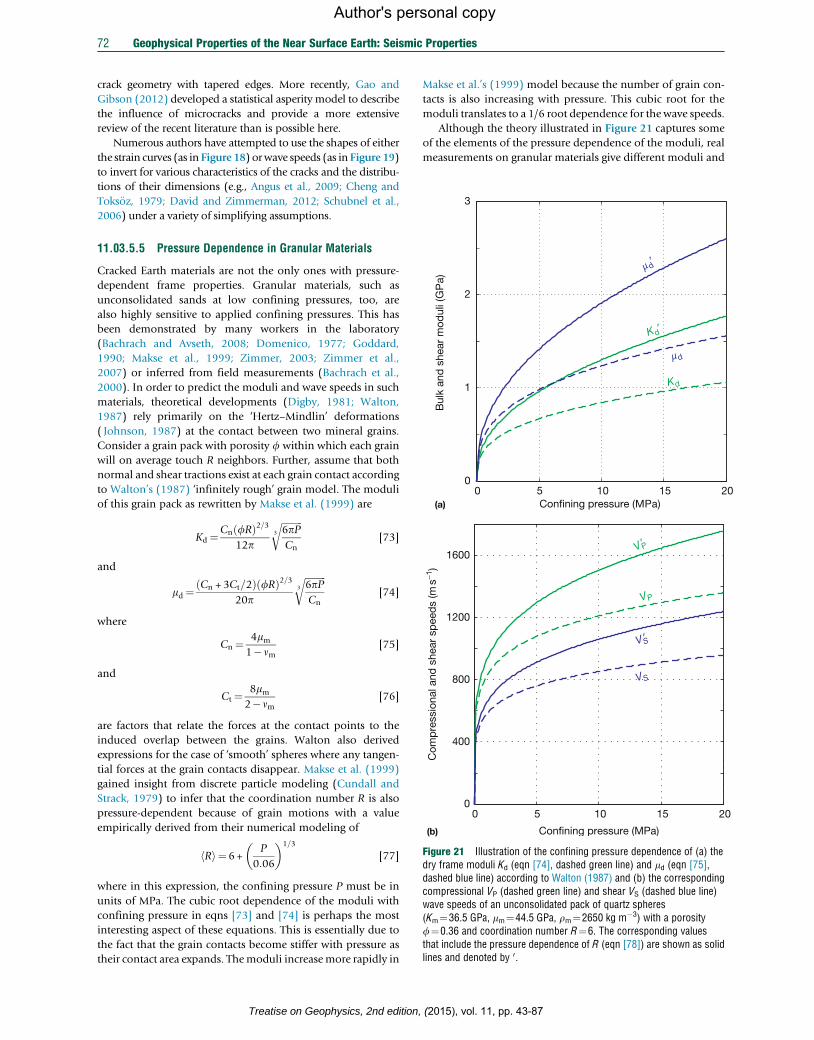
0
1
2
3
Confining pressure (MPa)
Bul
k an
d s
hear
mod
uli (
GP
a)
0 5 10 15 20(a)
VS′
VS
(b)
0 5 10 15 200
400
800
1200
1600
Confining pressure (MPa)
Com
pre
ssio
nal a
nd s
hear
sp
eed
s (m
s−1)
m d′
V P′
VP
Kd′
md
Kd
Figure 21 Illustration of the confining pressure dependence of (a) thedry frame moduli Kd (eqn [74], dashed green line) and md (eqn [75],dashed blue line) according to Walton (1987) and (b) the correspondingcompressional VP (dashed green line) and shear VS (dashed blue line)wave speeds of an unconsolidated pack of quartz spheres(Km¼36.5 GPa, mm¼44.5 GPa, rm¼2650 kg m�3) with a porosityf¼0.36 and coordination number R¼6. The corresponding valuesthat include the pressure dependence of R (eqn [78]) are shown as solidlines and denoted by 0.
72 Geophysical Properties of the Near Surface Earth: Seismic Properties
Author's personal copy
crack geometry with tapered edges. More recently, Gao and
Gibson (2012) developed a statistical asperity model to describe
the influence of microcracks and provide a more extensive
review of the recent literature than is possible here.
Numerous authors have attempted to use the shapes of either
the strain curves (as in Figure 18) orwave speeds (as in Figure 19)
to invert for various characteristics of the cracks and the distribu-
tions of their dimensions (e.g., Angus et al., 2009; Cheng and
Toks€oz, 1979; David and Zimmerman, 2012; Schubnel et al.,
2006) under a variety of simplifying assumptions.
11.03.5.5 Pressure Dependence in Granular Materials
Cracked Earth materials are not the only ones with pressure-
dependent frame properties. Granular materials, such as
unconsolidated sands at low confining pressures, too, are
also highly sensitive to applied confining pressures. This has
been demonstrated by many workers in the laboratory
(Bachrach and Avseth, 2008; Domenico, 1977; Goddard,
1990; Makse et al., 1999; Zimmer, 2003; Zimmer et al.,
2007) or inferred from field measurements (Bachrach et al.,
2000). In order to predict the moduli and wave speeds in such
materials, theoretical developments (Digby, 1981; Walton,
1987) rely primarily on the ‘Hertz–Mindlin’ deformations
( Johnson, 1987) at the contact between two mineral grains.
Consider a grain pack with porosity f within which each grain
will on average touch R neighbors. Further, assume that both
normal and shear tractions exist at each grain contact according
to Walton’s (1987) ‘infinitely rough’ grain model. The moduli
of this grain pack as rewritten by Makse et al. (1999) are
Kd ¼Cn fRð Þ2=312p
ffiffiffiffiffiffiffiffiffi6pPCn
3
r[73]
and
md ¼Cn + 3Ct=2ð Þ fRð Þ2=3
20p
ffiffiffiffiffiffiffiffiffi6pPCn
3
r[74]
where
Cn ¼ 4mm1� nm
[75]
and
Ct ¼ 8mm2� nm
[76]
are factors that relate the forces at the contact points to the
induced overlap between the grains. Walton also derived
expressions for the case of ‘smooth’ spheres where any tangen-
tial forces at the grain contacts disappear. Makse et al. (1999)
gained insight from discrete particle modeling (Cundall and
Strack, 1979) to infer that the coordination number R is also
pressure-dependent because of grain motions with a value
empirically derived from their numerical modeling of
Rh i¼ 6+P
0:06
� �1=3
[77]
where in this expression, the confining pressure P must be in
units of MPa. The cubic root dependence of the moduli with
confining pressure in eqns [73] and [74] is perhaps the most
interesting aspect of these equations. This is essentially due to
the fact that the grain contacts become stiffer with pressure as
their contact area expands. Themoduli increasemore rapidly in
Treatise on Geophysics, 2nd edition,
Makse et al.’s (1999) model because the number of grain con-
tacts is also increasing with pressure. This cubic root for the
moduli translates to a 1/6 root dependence for the wave speeds.
Although the theory illustrated in Figure 21 captures some
of the elements of the pressure dependence of the moduli, real
measurements on granular materials give different moduli and
(2015), vol. 11, pp. 43-87

x/a
-4 -3 -2 -1 0 1 2 3 44
3
2
1
0
-1
-2
-3
-4(a)
(b)
(c)
km s-1
km s-1
y/a
y
-4
-3
-2
-1
0
1
2
3
4
sxx sxx
44
44
33
33
22
22
11
11
33 22 11
VSH
V PO VP
VSV
VSO
Figure 22 Two-dimensional description of crack-induced elasticanisotropy. (a) Initial cracked medium with random orientation of cracks.(b) Distribution of remaining open cracks after application ofhorizontal compression stress sxx (modified from Schmitt DR,Currie CA, and Zhang L (2012) Crustal stress determination fromboreholes and rock cores: Fundamental principles. Tectonophysics580: 1–26). (c) Hypothetical wave velocity surfaces before (circlesoutlined with dashed lines) and after (solid lines) application of sxx.VPO and VSO are the original isotropic compressional and shear wavespeeds material of (a). VP, VSV, and VSH are the induced anisotropicwave surfaces for the compressional, the vertically polarized shear
Geophysical Properties of the Near Surface Earth: Seismic Properties 73
Treatise on Geophysics, 2nd editio
Author's personal copy
velocities (Hardin and Blandford, 1989). On the basis of an
extensive series of ultrasonic wave speed measurements on a
wide variety of different packs of synthetic and natural grains,
(Zimmer, 2003; Zimmer et al., 2007) found exponents that
were significantly <1/6. Recently, Andersen and Johansen
(2010) found that Walton’s (1987) model overpredicts the
observed sonic log wave speeds in unconsolidated sands by
more than a factor of 1.5, and they suggested empirically
derived curves (e.g., Fam and Santamarina, 1997) may be best.
11.03.5.6 Implications of Pressure Dependence
The pressure sensitivity of moduli and wave speeds has two
important implications. The first is that the application of
nonhydrostatic or deviatoric stress states affects the rock’s elas-
tic anisotropy. The second is that the properties are also highly
sensitive to a pore pressure. Both of these factors can strongly
affect the seismic observations.
11.03.5.6.1 Stress-induced anisotropy (acoustoelasticeffect)All of the discussions to this point have assumed that the
materials are subject to a uniform hydrostatic confining pres-
sure P. In the Earth, however, a deviatoric state of stress is the
general case. Such states of stress produce wave speed anisot-
ropy in both granular (Sayers, 2002, 2007; Walton, 1987) and
cracked (Horii and Nemat-Nasser, 1983; Sayers and Kachanov,
1995) rocks. In the former, the anisotropy results from the
stiffening of the contacts in the direction parallel to the greater
compression. In the latter, the anisotropy is primarily a conse-
quence of the preferred closure of those cracks whose plane is
aligned normal to the greatest principle compression. Nur and
Simmons (1969) may have been the first to observe these
phenomena although the stress concentrations in their circular
sample subject to a uniaxial force were not uniform. Since then
the effect has been documented by many workers under more
controlled stress state conditions (e.g., Babuska and Pros,
1984; Becker et al., 2007; Bonner, 1974; Gurevich et al.,
2011; Johnson and Rasolofosaon, 1996; Stanek et al., 2013)
in cracked rock, (Nur, 1971) in granular rock (e.g., Dillen et al.,
1999; Khidas and Jia, 2010; Prioul et al., 2004; Rai and
Hanson, 1988; Roesler, 1979) and numerically (Gallop,
2013; Hu et al., 2010). At the field scale, Schijns et al. (2012)
were able to explain the observed seismic anisotropy in a
1300 m thick section of the Outokumpu biotite gneiss on the
basis of oriented microcracks and mineral CPO (Elbra et al.,
2011; Kern et al., 2009; Lassila et al., 2010; Wenk et al., 2012).
The basis of this effect again derives from the progressive
closure of the crack-like porosity with compression. Consider
an unstressed rock mass containing numerous narrow cracks,
the orientations of which are randomly but uniformly distrib-
uted (Figure 22(a)). Application of an appropriately large
uniaxial stress sxx to the mass closes those cracks whose planes
are perpendicular or nearly so to the direction of sxx (Berg,
1965; Walsh, 1965) while leaving the cracks whose planes are
(i.e., in the plane of the figure), and the horizontally polarizedshear (i.e., perpendicular to the plane of the figure) wave modes,respectively. In (c), the wave speed is represented by the distancefrom the origin.
n, (2015), vol. 11, pp. 43-87

2000
2500
3000
3500
4000
4500
5000
Total confining pressure (MPa)
Ob
serv
ed w
ave
spee
ds
(ms-
1 )
V PV S
0 20 40 60
Peff= 30 Mpa
Peff= 30 Mpa
Peff= 15 Mpa
Peff= 15 Mpa
Figure 23 Observed ultrasonic velocities in a water-saturated sampleof the Cadotte sandstone (see Figure 19) versus the total confiningpressure. The solid lines are the velocities for VP (blue) and VS (red) forthe sample with a small and constant pore pressure. Dashed and dottedlines and open circles and squares indicate the observations when thedifferential pressure P�PP is held constant at either 15 or 30 MPa,respectively. Data for sample SB007 of He (2006).
74 Geophysical Properties of the Near Surface Earth: Seismic Properties
Author's personal copy
aligned to the stress open as shown in Figure 22(b). This
transforms the initially isotropic rock into a transversely iso-
tropic one (Fuck and Tsvankin, 2009) with directionally
dependent relative wave speeds as shown in Figure 22(c).
Stress-induced anisotropy is important in many geophysi-
cal problems from complicated stress conditions near a well-
bore (Schmitt et al., 1989; Winkler, 1996), in mines (Holmes
et al., 2000a; Holmes et al., 2000b), over petroleum reservoirs
(Wuestefeld et al., 2011), and in stress changes related to
seismicity. (Crampin, 1994; Crampin and Peacock, 2008) in
particular had championed the interpretation of shear wave
splitting to infer stress states for reservoir monitoring and
earthquake forecasting.
11.03.5.6.2 Influence of pore pressureAlthough we are not yet considering the effects on the dynamic
seismic properties of fluids in the pore space of the rocks, the
fluid pore pressure Pp has an important effect on the static
elastic properties of the frame that must be taken account of
in most cases. Numerous laboratory experiments have shown
that the frame properties of rocks depend not on the confining
pressure P per se but on the effective pressure Pe:
Pe ¼ P�xPp [78]
where x the pore pressure coefficient. More generally, for a set
of total or confining stresses sij, the effective stresses seij eqn[78] can be written as
seij ¼ sij�dijxPp [79]
where dij is the Kronecker delta; the pore fluid does not influ-
ence the shear stresses.
What this means is that the frame moduli Kd and md and
consequently the wave speeds VP and VS are generally func-
tions of Pe. A corollary to this is that the dry moduli do not
change (to the first approximation) if Pe remains constant. The
measurements of He (2006) on the Cadotte sandstone illus-
trate these effects well (Figure 23). In his tests, he first mea-
sured VP and VS through a water-saturated sample of the
Cadotte sandstone at confining pressures to 60 MPa while
maintaining the pore pressure Pp¼0. This yields the highly
nonlinear curve of velocities versus confining pressure as was
already encountered for a similar dry sample in Figure 19.
Once this was accomplished, He repeated the measurements
in suites where the differential pressure was held constant first
at 15 MPa and then at 30 MPa. In both of these, the wave
speeds remain constant, meaning that x¼1 over this pressure
range to within experimental error.
The concept of effective pressure can be confusing in part
because a worker must take care to consider which definition
of effective pressure one truly requires for the phenomena at
hand. More directly, this usually means one must have the
appropriate value of x for the physical process being studied
(Berryman, 1992; Berryman, 1993). The effective pressure/
stress concept was first developed by Terzaghi with x¼1. How-
ever, the apparent x will deviate from unity depending on the
rock structure and potential of chemical interaction (e.g., swell-
ing clays) (Bernabe, 1987; Zoback and Byerlee, 1975), on the
rates at which pore pressures can recharge during rapid defor-
mation and dilatancy leading to failure (Brace and Martin,
Treatise on Geophysics, 2nd edition,
1968; Schmitt and Zoback, 1992), and on the linear strains
and volumetric deformation of the material itself (Biot and
Willis, 1957; Nur and Byerlee, 1971). With regard to the last
item, the Biot–Willis effective stress coefficient for poroelastic
strain is
x¼ 1� Kd
Km[80]
Unfortunately, the use of eqn [80] in determining the
appropriate effective pressure or stress in determining VP or
VS has propagated through the rock physics literature. This
usage is incorrect, as emphasized by Mavko and Vanorio
(2010), and can lead to significant error particularly in com-
pressible materials. For purposes of finding moduli or wave
speeds, it is more proper to assume x�1 in the absence of
additional information on the material behavior.
The influence of effective pressure on seismic responses is of
particular interest in time-lapse seismology. Pore pressures Ppin reservoirs will vary as fluids are injected or produced and
this results in a change in the effective stress and, hence, VP and
VS and the consequent seismic reflectivity. Proper interpreta-
tion of time-lapse observations cannot easily ignore the
changes in the effective pressure or stress (Herwanger and
Horne, 2005; Sayers, 2004).
11.03.6 Seismic Waves in Fluid-Saturated Rocks
Most commonly, a worker requires a prediction of the seismic
wave speeds under the in situ conditions in the Earth where the
rock is subject to various stresses, pore pressures, and fluid
saturations. After providing information on the behavior of
(2015), vol. 11, pp. 43-87

Geophysical Properties of the Near Surface Earth: Seismic Properties 75
Author's personal copy
the rock’s various components of the mineral solid, the fluid,
and the rock’s frame in the preceding sections, we are now
ready to review the approaches to understanding the seismic
properties of fluid-saturated rocks. This is often referred to as a
fluid substitution analysis. To summarize, the building blocks
needed to determine the fluid-saturated bulk Ksat and shear msatmoduli that are necessary to calculate VP and VS with eqns [1]
and [2] are as follows:
• The elastic moduli Km and mm and density rm of the solid
mineral constituents.
• The saturating fluid’s adiabatic bulk modulus Kf and its
density rf. If velocity dispersion is included, then one
must also include the viscosity z.
• The rock frame’s elastic dry or drained elastic moduli Kd
and md and its porosity f. If frequency is considered, then
one must also include additional factors such as the tortu-
osity t, the permeability k, and somemeasure of the dimen-
sions of the pore.
Of course, one must remember that most of these depend
on stress, pressure, and temperature as discussed in the previ-
ous sections and the values need to be appropriately chosen for
the case at hand. After the intensive earlier discussions of
the various mineral, fluid, and frame properties, the fluid-
saturated expressions to come may seem anticlimactic. Often,
finding the appropriate values of the inputs may take the most
effort.
In this section, we review a number of the more important
expressions that allow for the calculation of the saturated rock
elastic moduli. This begins with Gassmann’s widely employed
formula and progresses through brief surveys of the local and
global flow models that account for frequency effects.
11.03.6.1 Gassmann’s Equation
Gassmann (1951) constructed expressions for the moduli of a
fluid-saturated porous material. These expressions are rela-
tively simple, and because of this, they are used almost exclu-
sively in practice. His development is essentially that for an
undrained poroelastic solid (Berryman, 1999; Rice and Cleary,
1976; Smith et al., 2003; Wang, 2000) and as such is strictly
valid for static deformations. In developing his equations, he
assumed the minerals and fluids interacted only mechanically,
that the material was fully saturated and isotropic, that it was
monomineralic, and, importantly, that the shear modulus is
not influenced by the pore fluid. This last assumption leads to
the expression for the saturated shear modulus msat
msat ¼ md [81]
and the saturated bulk modulus Ksat
Ksat ¼Kd +x2
fKf
+x�fKm
[82]
where x is the poroelastic pore pressure coefficient of eqn [80].
Gassmann looked at the problem more as a superposition of
interrelated volumetric strains of the frame, the minerals, and
the fluid. The same result can be found independently as the
undrained modulus from poroelasticity. Gassmann’s formulas
Treatise on Geophysics, 2nd editio
are written in many different ways, but one advantage of eqn
[82] is that it highlights that the fluid effects are essentially a
correction to Kd (Han and Batzle, 2004).
For the sake of convenience it is also worth rewriting an
inverted form of Gassmann’s equation [82]:
Kd ¼fKm
Kf+ 1�f
� �Ksat�Km
fKm
Kf�1�f +
Ksat
Km
[83]
which is particularly useful in estimating Kd from sonic log
information (Carcione et al., 2006).
Physically, the application of Gassmann’s equations [81]
and [82] assumes that during the passage of a wave over a small
(relative to the wavelength) but representative volume VR of
the saturated rock, the frequency is sufficiently low that the
pore pressure remains uniform throughout VR. With no varia-
tions in pressure, there can be no fluid exchange between VR
and its neighboring representative volumes.
There are a number of salient points arising from
Gassmann’s equations including the following:
i. Ksat�Kd. That is, a fluid-saturated rock is always less com-
pressible than the dry frame by itself.
ii. 1�x�0. The upper bound occurs as Kd vanishes for
increasingly compressible materials such as unconsolidated
sands. It is interesting to note by examination that as x!1,
Ksat approaches the Voigt bound equation [58] for the
mixture of fluid and solid. The lower bound is approached
as Kd!Km where the rock is very stiff. Consequently, the
influence of fluids diminishes as the frame stiffens.
iii. Km�Kf.. As Tables 1 and 2 show, typical mineral moduli
are mostly >30 GPa. In contrast, most typical liquid mod-
uli are �1–3 GPa and gas moduli are �0.1–100 MPa
(Table 3). As such, for real materials, Ksat is substantially
more sensitive to Kf than to Km. A corollary to this is that a
compressible fluid (i.e., gas) has less effect than does a
stiffer fluid (liquid).
iv. VS will decrease upon saturation. The decrease, although it
may only be small, occurs because, by definition, the shear
modulus does not change but the bulk density r as given in
eqns [55] and [56] must increase.
v. VP will usually, but not necessarily, increase upon satura-
tion. This increase is primarily due to the larger value of
Ksat. However, one must always keep in mind that rsat alsorises, and should rf be sufficiently large, it is quite possible
that VP will decrease upon saturation. This happens, for
example, with pure CO2 (e.g., see Njiekak et al., 2013).
It is worthwhile investigating the implications of
Gassmann’s equations. Figure 24(a) shows a suite of dry elas-
tic moduli that might represent the values for a number of
limestones with a range of porosities 0 f 0.4. Both Kd and
md decrease substantially with porosity as expected. Ksat is
calculated using eqn [82]; it is always greater than Kd but the
two continue to diverge from one another with porosity and
Ksat is nearly twice Kd once a porosity f¼0.35 is reached. The
dry and saturated shear moduli are exactly the same according
to Gassmann’s assumptions in eqn [81].
The seismic wave speeds may subsequently be calculated
using eqns [1] and [2] (Figure 24(b)). VS decreases a small
n, (2015), vol. 11, pp. 43-87

00
1000
2000
3000
4000
5000
6000
7000
Velo
city
(ms−1
)
0.1 0.2 0.3 0.4Porosity
0.2 0.3 0.4
Porosity
0.100
10
20
30
40
50
60
70
Mod
uli (
GP
a)
2
3
4
5
0 0.1 0.2 0.31
Porosity0.4
0.3
0.35
0.4
0.45
0.5
Poisson’s ratios
md =m
sat
VP/V
S R
atio
s
Ksat
Kd
VP sat
VSsat
VPdry
VSdry
V P/V S s
at
VP/VS dry
νsatνdry
(a)
(b)
(c)
Figure 24 Illustration of the application of Gassmann’s equations to aseries of hypothetical rocks of increasing porosity. (a) Comparison of
76 Geophysical Properties of the Near Surface Earth: Seismic Properties
Treatise on Geophysics, 2nd edition,
Author's personal copy
amount upon substitution because of the increase in the bulk
density as already noted. For this case, however, VP increases
relative to that for the dry frame; the increase in the bulk
modulus has managed to overwhelm the increase in the den-
sity. At the greater porosities (or equivalently smaller Kd), the
saturating water has a greater influence on VPsat. These differ-
ences would be further amplified for the acoustic impedances.
It is these types of differences that hold the key to the time-
lapse seismic surveying.
Figure 24(c) shows the two parameters that are often
derived from the wave speeds, the direct VP/VS ratio and
Poisson’s ratio equation [9]. These can serve as proxy indica-
tors of the saturation state of the rock in part because of the
relative impacts of saturation on VPsat and VSsat. For example,
the VP/VS ratio for water saturation is substantially greater than
that for the dry (or nearly equivalently gas-filled) conditions.
This difference is even greater for Poisson’s ratio n with a larger
Poisson’s ratio, indicating liquid saturation.
11.03.6.2 Frequency-Dependent Models
Gassmann’s equations remain popular, but as noted, they
strictly apply only under static conditions. However, in
reality, researchers must work over a large range of frequencies.
In the broadest sense, ‘seismic’ investigations center on fre-
quencies of 1 MHz, 10 kHz, and 100 Hz for ultrasonic labora-
tory measurements, borehole sonic log readings, and applied
seismic investigations, respectively.
In the laboratory, Gassmann’s equations rarely reproduce
the observed wave speeds particularly at low confining pres-
sures. An example of this, again taken from measurements on
the Cadotte sandstone (He, 2006), is given in Figure 25 that
shows the observed dry and water-saturated measurements as a
function of the effective confining pressure. The observed VPsat
are greater than VPdry as expected but they exceed those values
predicted using Gassmann’s equations significantly. Similar
anomalies are seen for VSsat that again is much greater than
VSdry; this is in opposition to Gassmann’s predicted values that
are slightly smaller than VSdry because of the increased density
of the bulk saturatedmaterial. It is important to note that as the
crack-like porosity closes, the observed and predicted values
begin to approach one another. Indeed, even at the pressure of
only 60 MPa, VSsat has nearly intersected with VSdry. Clearly,
there is a large discrepancy between the observed and predicted
saturated wave speeds particularly at the low confining pres-
sures where the cracks remain most open (see also Mavko and
Jizba (1991) for similar evidence).
An extreme case of wave speed dispersion is seen from
recent VP and VS measurements through a highly porous,
CO2-saturated medium of sintered alumina (Yam, 2011; Yam
and Schmitt, 2011). Figure 26 shows the variations of the
observed ultrasonic (1 MHz) VPsat and VSsat with pore pressure
Pp for a suite of measurements carried out at constant differ-
ential effective stress Peff¼P�Pp of 15 MPa. As noted in the
the dry frame modulus bulk Kd (blue) to the saturated bulk modulus Ksat.Note that by definition, the dry md and saturated msat shear moduli areequal. (b) Corresponding compressional and shear waves speeds forthe dry and saturated cases. (c) Corresponding VP/VS and Poisson’sratios for the dry and saturated cases.
(2015), vol. 11, pp. 43-87

2000
2500
3000
3500
4000
4500
5000
Total confining pressure (MPa)
Ob
serv
ed a
nd p
red
icte
d w
ave
spee
ds
(m s
−1)
0 20 40 60
V Sdr
y
V Ssa
t
V Psa
t
V Pdr
y
Figure 25 Observed VP (blue) and VS (red) wave speeds in Cadottesandstone SB007 for dry (filled squares) and water-saturated (filledcircles) situations. Theoretical Gassmann’s wave speeds calculated usingthe dry moduli are also shown as lines.
10 15 20 25 30
3200
3300
3400
3500
3600
3700
1900
2000
2100
2200
2300
Pore fluid pressure (MPa)Lo
ngitu
din
al w
ave
spee
d (m
s− 1)
Tran
sver
se w
ave
spee
d (m
s−1)
Gas Liquid
Biot
Biot
0 5
Figure 26 Comparison of observed ultrasonic wave speeds in aCO2-saturated porous sintered alumina held at a constant differentialpressure of Peff¼15 MPa and temperature T¼28 ºC. The porepressure is varied in order to effect the gas–liquid phase transition thatoccurs at 6.144 MPa. Observed values of VPsat and VSsat are indicatedby red upside down triangles. Calculated values of the wave speedsaccording to the Biot formulations at 100 and 1 MHz are shown asdashed and solid black lines, respectively. For this case, the fluidsubstitution calculations using Gassmann’s zero frequency equationscannot be distinguished from the 100 Hz Biot calculations. Theviolet-filled zones indicate the range of wave speed dispersion that existsbetween 100 Hz (Gassmann) and 1 MHz (Biot). Data and calculationsfrom Yam (2011).
Geophysical Properties of the Near Surface Earth: Seismic Properties 77
Author's personal copy
preceding text, carrying out the measurements at constant
differential pressure should minimize any pressure-dependent
effects of the rock frame of wave speeds and most of
the variation will be due to changes in the fluid properties.
Figure 26 also shows the corresponding wave speeds predicted
by Gassmann’s equations from fluid substitution calculations
that employ knowledge of the fluid, solid, and dry frame
properties. Gassmann’s predictions are always less than the
observations. This difference is relatively small when CO2 gas
saturates the pores but it grows to over 6% when the CO2 is in
the liquid state.
In the case shown, the differences between the observed
and the predicted wave speeds at low frequencies arise primar-
ily because the latter does not account for differential motions
between the solid and fluid as the wave passes. We briefly
survey the two main models in the succeeding text that do
admit fluid motions. These are usually referred to as the global
and local flow models.
11.03.6.2.1 Global flow (biot) modelBuilding on his work in the consolidation of porous media, Biot
(1956a,b) constructed a seminalmodel to account for frequency-
dependent wave propagation through a fluid-saturated porous
and permeable medium. A full description of the model is
beyond the needs here but readers can find more information
in numerous contributions (Bourbie et al., 1987; Johnson, 1984;
Smeulders, 2005). A most interesting outcome of this theory is
that a third ‘slow’ longitudinal wave mode P2 exists in such
porous media because the fluid and solid are allowed to move
independently of one another. This out-of-phase motion
Treatise on Geophysics, 2nd editio
between the two admits a newdegree of freedom to the equations
of which the slow wave speed is the consequence.
This wave mode is difficult to observe in nature because the
differential fluid–solid motions result in large viscous losses.
Plona (1980) first observed this wave in acoustic refraction
experiments through highly porous sintered glass beads.
Figure 27 shows the results from similar recently conducted
tests (Bouzidi and Schmitt, 2009) that highlight well the exis-
tence of all three modes. It is interesting to note the loss of the
fast P1 wave past its critical angle. The P2 mode, which travels
substantially more slowly than the surrounding water, has no
critical angle and exists at all angles.
At this point, it is important to return to the CO2-saturated
measurements of Figure 26 where the Biot model has been
used to predict the observed VPsat and VSsat. The theory and
observations match well as the observed and calculated values
of VSsat agree to within experimental uncertainty. Those for
VPsat are only 20 m s�1 different. This agreement strongly sug-
gests that the Biot model and its low-frequency limit given by
Gassmann’s equations adequately predict the behavior with
frequency in highly porous and permeable materials. Although
not shown here, the Biot formulas also allowed attenuation to
be modeled satisfactorily (Yam, 2011).
n, (2015), vol. 11, pp. 43-87
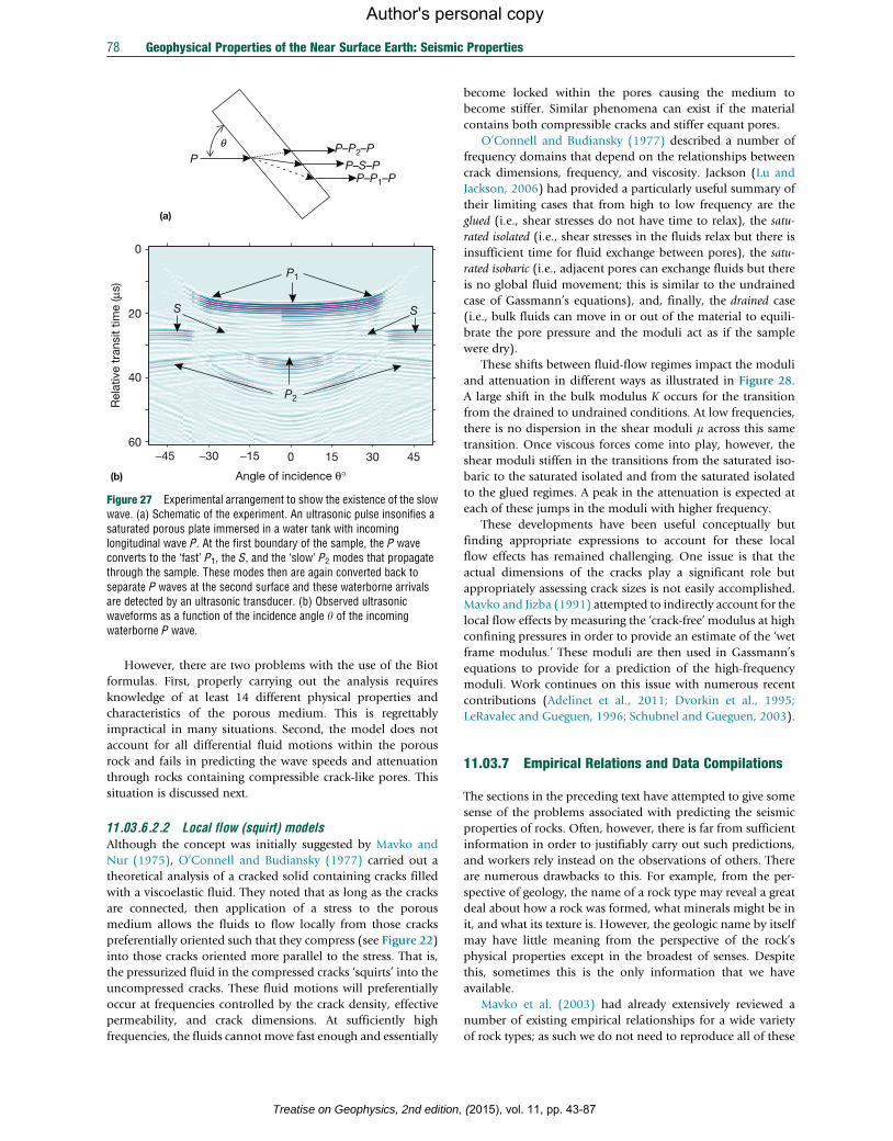
P–S–PP–P1–P
P–P2–PP
P1
P2
S S
Angle of incidence θ°
Rel
ativ
e tr
ansi
t tim
e ( μ
s)
0
20
40
60
q
−45 −30 0−15 15 30 45
(a)
(b)
Figure 27 Experimental arrangement to show the existence of the slowwave. (a) Schematic of the experiment. An ultrasonic pulse insonifies asaturated porous plate immersed in a water tank with incominglongitudinal wave P. At the first boundary of the sample, the P waveconverts to the ‘fast’ P1, the S, and the ‘slow’ P2 modes that propagatethrough the sample. These modes then are again converted back toseparate P waves at the second surface and these waterborne arrivalsare detected by an ultrasonic transducer. (b) Observed ultrasonicwaveforms as a function of the incidence angle y of the incomingwaterborne P wave.
78 Geophysical Properties of the Near Surface Earth: Seismic Properties
Author's personal copy
However, there are two problems with the use of the Biot
formulas. First, properly carrying out the analysis requires
knowledge of at least 14 different physical properties and
characteristics of the porous medium. This is regrettably
impractical in many situations. Second, the model does not
account for all differential fluid motions within the porous
rock and fails in predicting the wave speeds and attenuation
through rocks containing compressible crack-like pores. This
situation is discussed next.
11.03.6.2.2 Local flow (squirt) modelsAlthough the concept was initially suggested by Mavko and
Nur (1975), O’Connell and Budiansky (1977) carried out a
theoretical analysis of a cracked solid containing cracks filled
with a viscoelastic fluid. They noted that as long as the cracks
are connected, then application of a stress to the porous
medium allows the fluids to flow locally from those cracks
preferentially oriented such that they compress (see Figure 22)
into those cracks oriented more parallel to the stress. That is,
the pressurized fluid in the compressed cracks ‘squirts’ into the
uncompressed cracks. These fluid motions will preferentially
occur at frequencies controlled by the crack density, effective
permeability, and crack dimensions. At sufficiently high
frequencies, the fluids cannot move fast enough and essentially
Treatise on Geophysics, 2nd edition,
become locked within the pores causing the medium to
become stiffer. Similar phenomena can exist if the material
contains both compressible cracks and stiffer equant pores.
O’Connell and Budiansky (1977) described a number of
frequency domains that depend on the relationships between
crack dimensions, frequency, and viscosity. Jackson (Lu and
Jackson, 2006) had provided a particularly useful summary of
their limiting cases that from high to low frequency are the
glued (i.e., shear stresses do not have time to relax), the satu-
rated isolated (i.e., shear stresses in the fluids relax but there is
insufficient time for fluid exchange between pores), the satu-
rated isobaric (i.e., adjacent pores can exchange fluids but there
is no global fluid movement; this is similar to the undrained
case of Gassmann’s equations), and, finally, the drained case
(i.e., bulk fluids can move in or out of the material to equili-
brate the pore pressure and the moduli act as if the sample
were dry).
These shifts between fluid-flow regimes impact the moduli
and attenuation in different ways as illustrated in Figure 28.
A large shift in the bulk modulus K occurs for the transition
from the drained to undrained conditions. At low frequencies,
there is no dispersion in the shear moduli m across this same
transition. Once viscous forces come into play, however, the
shear moduli stiffen in the transitions from the saturated iso-
baric to the saturated isolated and from the saturated isolated
to the glued regimes. A peak in the attenuation is expected at
each of these jumps in the moduli with higher frequency.
These developments have been useful conceptually but
finding appropriate expressions to account for these local
flow effects has remained challenging. One issue is that the
actual dimensions of the cracks play a significant role but
appropriately assessing crack sizes is not easily accomplished.
Mavko and Jizba (1991) attempted to indirectly account for the
local flow effects by measuring the ‘crack-free’ modulus at high
confining pressures in order to provide an estimate of the ‘wet
frame modulus.’ These moduli are then used in Gassmann’s
equations to provide for a prediction of the high-frequency
moduli. Work continues on this issue with numerous recent
contributions (Adelinet et al., 2011; Dvorkin et al., 1995;
LeRavalec and Gueguen, 1996; Schubnel and Gueguen, 2003).
11.03.7 Empirical Relations and Data Compilations
The sections in the preceding text have attempted to give some
sense of the problems associated with predicting the seismic
properties of rocks. Often, however, there is far from sufficient
information in order to justifiably carry out such predictions,
and workers rely instead on the observations of others. There
are numerous drawbacks to this. For example, from the per-
spective of geology, the name of a rock type may reveal a great
deal about how a rock was formed, what minerals might be in
it, and what its texture is. However, the geologic name by itself
may have little meaning from the perspective of the rock’s
physical properties except in the broadest of senses. Despite
this, sometimes this is the only information that we have
available.
Mavko et al. (2003) had already extensively reviewed a
number of existing empirical relationships for a wide variety
of rock types; as such we do not need to reproduce all of these
(2015), vol. 11, pp. 43-87
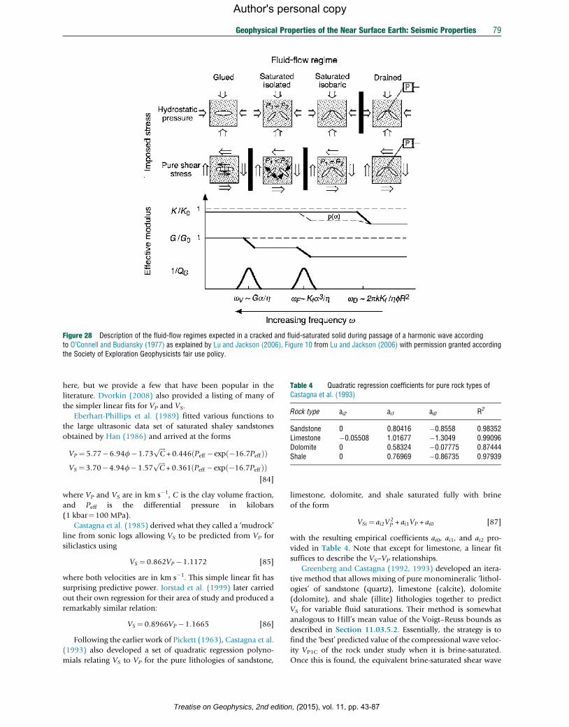
Figure 28 Description of the fluid-flow regimes expected in a cracked and fluid-saturated solid during passage of a harmonic wave accordingto O’Connell and Budiansky (1977) as explained by Lu and Jackson (2006). Figure 10 from Lu and Jackson (2006) with permission granted accordingthe Society of Exploration Geophysicists fair use policy.
Table 4 Quadratic regression coefficients for pure rock types ofCastagna et al. (1993)
Rock type ai2 ai1 ai0 R2
Sandstone 0 0.80416 �0.8558 0.98352Limestone �0.05508 1.01677 �1.3049 0.99096Dolomite 0 0.58324 �0.07775 0.87444Shale 0 0.76969 �0.86735 0.97939
Geophysical Properties of the Near Surface Earth: Seismic Properties 79
Author's personal copy
here, but we provide a few that have been popular in the
literature. Dvorkin (2008) also provided a listing of many of
the simpler linear fits for VP and VS.
Eberhart-Phillips et al. (1989) fitted various functions to
the large ultrasonic data set of saturated shaley sandstones
obtained by Han (1986) and arrived at the forms
VP ¼ 5:77�6:94f�1:73ffiffiffiffiC
p+ 0:446 Peff �exp �16:7Peffð Þð Þ
VS ¼ 3:70�4:94f�1:57ffiffiffiffiC
p+0:361 Peff �exp �16:7Peffð Þð Þ
[84]
where VP and VS are in km s�1, C is the clay volume fraction,
and Peff is the differential pressure in kilobars
(1 kbar¼100 MPa).
Castagna et al. (1985) derived what they called a ‘mudrock’
line from sonic logs allowing VS to be predicted from VP for
siliclastics using
VS ¼ 0:862VP �1:1172 [85]
where both velocities are in km s�1. This simple linear fit has
surprising predictive power. Jorstad et al. (1999) later carried
out their own regression for their area of study and produced a
remarkably similar relation:
VS ¼ 0:8966VP�1:1665 [86]
Following the earlier work of Pickett (1963), Castagna et al.
(1993) also developed a set of quadratic regression polyno-
mials relating VS to VP for the pure lithologies of sandstone,
Treatise on Geophysics, 2nd editio
limestone, dolomite, and shale saturated fully with brine
of the form
VSi ¼ ai2V2P + ai1VP + ai0 [87]
with the resulting empirical coefficients ai0, ai1, and ai2 pro-
vided in Table 4. Note that except for limestone, a linear fit
suffices to describe the VS–VP relationships.
Greenberg and Castagna (1992, 1993) developed an itera-
tive method that allows mixing of pure monomineralic ‘lithol-
ogies’ of sandstone (quartz), limestone (calcite), dolomite
(dolomite), and shale (illite) lithologies together to predict
VS for variable fluid saturations. Their method is somewhat
analogous to Hill’s mean value of the Voigt–Reuss bounds as
described in Section 11.03.5.2. Essentially, the strategy is to
find the ‘best’ predicted value of the compressional wave veloc-
ity VP1C of the rock under study when it is brine-saturated.
Once this is found, the equivalent brine-saturated shear wave
n, (2015), vol. 11, pp. 43-87

80 Geophysical Properties of the Near Surface Earth: Seismic Properties
Author's personal copy
velocity is calculated using the empirical regressions of Equa-
tion [87] just described. With knowledge of the brine-saturated
density, one can easily calculate the rock’s shear modulus mdthat in turn can be used to calculate the proper shear wave
velocity for the saturation at the proper saturation state using
the rock’s density rsat.Hence, the basis of the method is to make a proper estimate
of VP1C. To carry this out, one must have appropriate knowl-
edge of the rock’s porosity f, its in situ saturations Sw, So,
and Sg (see eqns [56] and [57]), and its observed in situ com-
pressional velocity VPsat. Further, the solid volume fractions Xi
of the L different ‘lithologies’
XLi¼0
Xi ¼ 1 [88]
forming the rock’s frame must also be found.
In the Greenberg and Castagna method, they first guess a
value of the compressional wave speed VP1C for the rock fully
saturated with brine (i.e., Sw¼1). With the guess VP1C, one
can directly calculate the expected values VSi for each of the
lithologies using eqn [87] and Table 4. Using these VSi,
the shear wave velocity for the brine-saturated rock VS1C is
calculated in a manner analogous to the Voigt–Reuss–Hill
calculations:
VS1C ¼ 1
2
XLi¼0
XiVSi
" #+XLi¼0
Xi
VSi
" #�1( )[89]
The density of the brine-saturated rock r1C is calculated
using an adaptation of eqn [55]:
r1C ¼frw + 1�fð ÞXLi¼1
Xirmi [90]
where the brine density must be determined for the appropriate
conditions as discussed in Section 11.03.4.3.2.1. Note that the
Greenberg and Castagna (1992) lithologies are sandstone, lime-
stone, dolomite, and shale. The mineral densities rmi that they
employed for these lithologies are, respectively, those for quartz,
calcite, dolomite, and illite as could be obtained from Table 2.
The in situ saturated density rsat can be either directly observed
or calculated with an additional adaptation of eqn [56]:
rsat ¼fXnj¼1
Sjrfj
!+ 1�fð Þ
XLi¼1
Xirmi [91]
With the values of VS1C and r1C, the drained shear modulus
md using eqn [2]
md ¼V2S1Cr1C [92]
may be calculated. The saturated bulk modulus Ksat of the rock
in situ with its proper saturation is then from eqn [1]:
Ksat ¼V2Psatrsat�
4
3md [93]
The drained frame modulus Kd may then be determined
using the inverse Gassmann’s equation [83] with knowledge of
the appropriate Kf for the pore fluids and Km for the mineral
solids discussed in earlier sections. Now, the calculations are
run somewhat backward in order to provide an updated value
for the fully brine-saturated (Sw¼1) compressional wave speed
V 0P1C using eqn [1]:
Treatise on Geophysics, 2nd edition,
V 0P1C ¼ Kd +
x2
fKw
+ x�fKm
!+4
3md
" #r�11C
( )1=2
[94]
with the bulk modulus of the brine Kw taking the place of Kf in
Gassmann’s equation [82]. V 0P1C can then be used as the new
VP1C and the calculation repeated. This process can iterate until
V 0P1C and VP1C converge within acceptable limits. Once the
convergence is complete, the current value of md is accepted
and the final estimate of the shear wave velocity VSsat is simply
calculated using eqn [2]:
VSsat ¼ffiffiffiffiffiffiffimdrsat
r[95]
Raymer et al. (1980) also using well log information devel-
oped a piecewise relationship to predict velocity from knowl-
edge of porosity and the intrinsic compressional wave speeds
VPm and Vf for the constituent mineral and solid, respectively.
This formula is
VP ¼ 1�fð Þ2VPm +fVf , f< 0:37
1
rV2P
¼ frf V
2f
+1�frmV
2Pm
, f> 0:47
1
VP¼ 0:47�f
0:10
1
V37+f�0:37
0:10
1
V47, 0:37<f< 0:47
[96]
where V37 and V47 are the velocities of the saturated rock for
f¼37% and f¼47%, respectively. Dvorkin (2008) more
recently came up with a similar relation to predict shear wave
velocities:
VS ¼ 1�fð Þ2VSm1�fð Þrm
1�fð Þrm +frf
� �[97]
given knowledge of the intrinsic mineral shear wave velocity
VSm and the fluid and intrinsic mineral densities, rf and rm,respectively.
Hamilton (1979) derived a number of expressions for
velocities in marine sediments (primarily silt–clays, turbidites,
and mudstone shales); one of these relates VP (in km s�1) to
depth D (in km) by
VP ¼ 1:511+ 1:304D�0:741D2 + 0:257D3 [98]
which is accurate to about 800 m depth.
The general empirical relationship between density and
seismic velocity fit by Gardner et al. (Gardner et al., 1974;
Sayers and den Boer, 2011) is still widely applied in seismic
studies particularly if only one of the other logs is available
from a borehole
r� 1:741V0:25P [99]
with VP in km s�1 and r in g cm�3.
More recently, Christensen and Stanley (2003) carried out a
fit of VP and VS versus r from a compilation of laboratory
measurements on a variety of igneous, metamorphic, and sed-
imentary rocks yielding
VP ¼ 2:8r�1:5752 [100]
and
VS ¼ 1:4r�0:4019 [101]
where again the velocities are in km s�1 and r in g cm�3.
(2015), vol. 11, pp. 43-87

Geophysical Properties of the Near Surface Earth: Seismic Properties 81
Author's personal copy
Examination of these regressions shows that, for the most
part, they do not contain any physical principles. Hence, the
reader must take care when applying these formulas and know
their limitations.
Compilations of observed values of velocities and densities
are also important sources of information. The densities of
rocks and minerals are covered extensively by Wohlenberg
(1982), while in the same series, Gebrande (1982) and Kern
(1982) provided exhaustive listings of wave speeds as func-
tions of pressure for various rock types. Christensen (1982,
1989) had provided the results of thousands of ultrasonic
velocity laboratory measurements that have been used to create
sophisticated models of the continental crust (Christensen and
Mooney, 1995). Ji et al.’s (2002) compilation is perhaps the
most complete in that it contains the results of both modeling
and measurements for a wide variety of different rock types.
Most recently, Gercek (2007) had compiled values of Poisson’s
ratio for a number of different Earth materials.
11.03.8 The Road Ahead
Studies related to ‘seismic properties’ continue to rapidly
expand, and in reality, each of the topics touched on in the
preceding text could be easily be turned into textbooks on their
own. In writing such a review, some important issues were
overlooked. The listing in the succeeding text contains impor-
tant directions of investigation that I believe will be of increas-
ing importance in the coming decade. These include the
following:
i. Seismic anisotropy was touched on only in the context of
mineral properties, but in general, rock is an anisotropic
medium. Since the 1980s, geophysicists have dominated
the literature on elastic anisotropy. As noted earlier, we do
not really have a good understanding of the anisotropy of
‘shales.’ This is in part because the physical properties of
clay mineralogical constituents are still not well known.
Characterizing the clay mineralogy within a given sample
remains problematic. The clay minerals themselves are dif-
ficult to study as the ‘crystals’ are often no more than a few
nanometers in dimension. The effects of cracks and frac-
tures on seismic responses still remain elusive. Being able to
deconvolve seismic observations to detect and characterize
fractures remains a goal for the future.
ii. Although it has been hinted at in the discussions earlier in
the text, we currently do not have a good handle on seismic
velocity dispersion in the Earth. Progress in this field
should come more rapidly with the development of a vari-
ety of forcing-function stress–strain techniques that can
allow the complex elastic moduli to be found at seismic
frequencies.
iii. We have seen earlier that most rocks display nonlinear
stress–strain or stress–velocity behavior. Despite this, we
still cling to attempting to analyze much of our observed
seismic data under the linearly elastic assumption. Cur-
rently, only a handful of workers are studying the often
unexpected effects of wave propagation in nonlinear mate-
rials. It is likely that this field can gain from the much larger
community of workers in nonlinear optics.
Treatise on Geophysics, 2nd editio
iv. In the laboratory, we often work on decimeter-scale sam-
ples that appear uniform and homogeneous. We then
attempt to extend this assumption of homogeneity to
much larger scales over many tens of meters (about the
seismic wavelengths). However, there are subtle dispersion
effects introduced by the scale of the heterogeneity of a rock
mass relative to the interrogating seismic waves. For exam-
ple, we most usually work under the ray theory paradigm
that assumes the wavelengths are small relative to the
dimensions of the heterogeneity. This is likely only rarely
true, and in many cases, the waves we observe may more
actually be revealing an effective medium. Much work
remains to be done on assessing to what degree effective
medium concepts may need to be incorporated to our field
observations.
v. Finally, the remarkable growth in computing power and in
easily employed parallel multiphysics numerical modeling
together with parallel technical developments in benchtop
x-ray tomography systems with micrometer-scale resolving
power is leading to the rapid growth of ‘digital rock
physics.’ These techniques allow one to calculate a variety
of physical properties from the 3-D microtomograms. Esti-
mation of electrical conductivity and permeability has been
most successful so far, but accurate predictions of the elastic
moduli and wave speeds have not yet been adequately
solved. This is in part because for the most part, workers
have focused on continuum approaches to solving such
problems. Now, however, one can build actual models
mimicking the true architecture of the minerals and pore
space and more thought needs to go on with regard to
actual physical phenomena in porous media at that scale
before the seismic properties can be adequately modeled.
Taken together, there still remains a great deal to learn with
regard to seismic properties of rocks. The new computational,
imaging, and experimental tools now at our disposal will allow
for rapid progress over the next decade.
Acknowledgments
The help of the many graduate students, postdoctoral
researchers, and technical staff in making many of the mea-
surements described in the preceding text is greatly appreci-
ated. DRS is supported by the Canada Research Chairs
Program. The author thanks T. Smith and the Editor L. Slater
for providing ideas on improving the manuscript.
References
Adams LH and Williamson ED (1923) On the compressibility of minerals and rocks athigh pressures. Journal of the Franklin Institute 195: 475–529.
Adelinet M, Fortin J, and Gueguen Y (2011) Dispersion of elastic moduli in a porous-cracked rock: Theoretical predictions for squirt-flow. Tectonophysics503: 173–181.
Alam MM, Fabricius IL, and Christensen HF (2012) Static and dynamic effective stresscoefficient of chalk. Geophysics 77: L1–L11.
Alexandrov KS and Ryzhova TV (1961a) The elastic properties of rock forming mineralsI: Pyroxenes and amphiboles. Bulletin (izvestiya), Academy of Sciences, USSR.Geophysics Series, vol. 9, pp. 871–875.
Alexandrov KS and Ryzhova TV (1961b) The elastic properties of rock forming mineralsII: Layered silicates. Bulletin (izvestiya), Academy of Sciences, USSR. GeophysicsSeries, vol. 12, pp. 1799–1804.
n, (2015), vol. 11, pp. 43-87

82 Geophysical Properties of the Near Surface Earth: Seismic Properties
Author's personal copy
Alexandrov KS and Ryzhova TV (1962) The elastic properties of rock forming mineralsIII: Feldspars. Bulletin (izvestiya), Academy of Sciences, USSR. Geophysics Series,vol. 2, pp. 186–189.
Alexandrov KS and Ryzhova TV (1964) The elastic properties of pyroxenes. SovietPhysics – Crystallography 8: 589–591.
Almqvist BSG, Burlini L, Mainprice D, and Hirt AM (2010) Elastic properties ofanisotropic synthetic calcite-muscovite aggregates. Journal of GeophysicalResearch, Solid Earth 115: B08203.
Andersen CF and Johansen TA (2010) Test of rock physics models for prediction ofseismic velocities in shallow unconsolidated sands: A well log data case.Geophysical Prospecting 58: 1083–1098.
Anderson OL (1963) A simplified method for calculating debye temperature from elasticconstants. Journal of Physics and Chemistry of Solids 24: 909–917.
Angel RJ, Jackson JM, Reichmann HJ, and Speziale S (2009) Elasticity measurementson minerals: A review. European Journal of Mineralogy 21: 525–550.
Angus DA, Verdon JP, Fisher QJ, and Kendall JM (2009) Exploring trends inmicrocrack properties of sedimentary rocks: An audit of dry-core velocity-stressmeasurements. Geophysics 74: E193–E203.
Auld BA (1990) Acoustic Fields and Waves in Solids, 2nd edn., p. 432. New York: JohnWiley and Sons.
Auzende AL, Pellenq RJM, Devouard B, Baronnet A, and Grauby O (2006) Atomisticcalculations of structural and elastic properties of serpentine minerals: The case oflizardite. Physics and Chemistry of Minerals 33: 266–275.
Azeemuddin M, Scott TE, Zaman M, and Roegiers JC (2001) Stress-Dependent Biot’sConstant Through Dynamic Measurements on Ekofisk Chalk. Paper presented at38th Symposium on Rock Mechanics: DC Rocks 2001. New York: Balkema.
Babuska V (1972) Elasticity and anisotropy of dunite and bronzitite. Journal ofGeophysical Research 77: 6955–6965.
Babuska V and Cara M (1991) Seismic Anisotropy in the Earth. Netherlands: Springer.Babuska V and Pros Z (1984) Velocity anisotropy in granodiorite and quartzite due to
the distribution of microcracks. Geophysical Journal of the Royal AstronomicalSociety 76: 113–119.
Bachrach R and Avseth P (2008) Rock physics modeling of unconsolidated sands:Accounting for nonuniform contacts and heterogeneous stress fields in the effectivemedia approximation with applications to hydrocarbon exploration. Geophysics73: E197–E209.
Bachrach R, Dvorkin J, and Nur AM (2000) Seismic velocities and poisson’s ratio ofshallow unconsolidated sands. Geophysics 65: 559–564.
Bailey E and Holloway JR (2000) Experimental determination of elastic properties of talcto 800 degrees C, 0.5 GPa; Calculations of the effect on hydrated peridotite, andimplications for cold subduction zones. Earth and Planetary Science Letters183: 487–498.
Bakhorji A (2009) Laboratory Measurements of Static and Dynamic Elastic Properties inCarbonate. PhD, University of Alberta.
Bass JD (1995) Elasticity of minerals, glasses, and melts. In: Ahrens TJ (ed.) MineralPhysics and Crystallography: A Handbook of Physical Constants, pp. 45–63.Washington, DC: American Geophysical Union.
Batzle M and Wang ZJ (1992) Seismic properties of pore fluids. Geophysics57: 1396–1408.
Becker K, Shapiro SA, Stanchits S, Dresen G, and Vinciguerra S (2007) Stress inducedelastic anisotropy of the Etnean basalt: Theoretical and laboratory examination.Geophysical Research Letters 34: L11307.
Behura J, Batzle M, Hofmann R, and Dorgan J (2007) Heavy oils: Their shear story.Geophysics 72: E175–E183.
Belogol’skii VA, Sekoyan SS, Samorukova LM, Stefanov SR, and Levtsov VI (1999)Pressure dependence of the sound velocity in distilled water. MeasurementTechniques 42: 406–413.
Benedict M, Webb GB, and Rubin LC (1942) An empirical equation for thermodynamicproperties of light hydrocarbons and their mixtures II. Mixtures of methane, ethane,propane, and n-butane. Journal of Chemical Physics 10: 747–758.
Benedict M, Webb GB, and Rubin LC (1951) An empirical equation for thermodynamicproperties of light hydrocarbons and their mixtures – Constants for12 hydrocarbons. Chemical Engineering Progress 47: 419–422.
Berg CA (1965) Deformation of fine cracks under high pressure and shear. Journal ofGeophysical Research 70: 3447–3452.
Berge PA, Bonner BP, and Berryman JG (1995) Ultrasonic velocity porosityrelationships for sandstone analogs made from fused glass-beads. Geophysics60: 108–119.
Bernabe Y (1987) The effective pressure law for permeability during pore pressure andconfining pressure cycling of several crystalline rocks. Journal of GeophysicalResearch-Solid Earth and Planets 92: 649–657.
Berryman JG (1992) Effective stress for transport-properties of inhomogeneous porousrock. Journal of Geophysical Research, Solid Earth 97: 17409–17424.
Treatise on Geophysics, 2nd edition,
Berryman JG (1993) Effective-stress rules for pore-fluid transport in rocks containing 2minerals. International Journal of Rock Mechanics and Mining Sciences &Geomechanics Abstracts 30: 1165–1168.
Berryman JG (1995) Mixture theories for rock properties. In: Rock Physics & PhaseRelations, pp. 205–228. Washington, DC: American Geophysical Union.
Berryman JG (1999) Origin of gassmann’s equations. Geophysics 64: 1627–1629.Berryman JG (2005) Bounds and self-consistent estimates for elastic constants of
random polycrystals with hexagonal, trigonal, and tetragonal symmetries. Journal ofthe Mechanics and Physics of Solids 53: 2141–2173.
Berryman JG (2012) Evaluating bounds and estimators for constants of randompolycrystals composed of orthotropic elastic materials. International Journal ofEngineering Science 58: 11–20.
Berryman JG and Berge PA (1996) Critique of two explicit schemes for estimatingelastic properties of multiphase composites. Mechanics of Materials 22: 149–164.
Berryman JG, Pride SR, and Wang HF (2002) A differential scheme for elastic propertiesof rocks with dry or saturated cracks. Geophysical Journal International151: 597–611.
Bett KE, Rowlinson JS, and Saville G (2003) Thermodynamics for Chemical Engineers.Cambridge: MIT Press.
Bianco E, Kaplan S, and Schmitt DR (2010) Seismic rock physics of steam injection inbituminous-oil reservoirs – Chapter 6. In: Batzle ML, Chopra S, Lines LR, andSchmitt DR (eds.) Heavy Oils: Reservoir Characterization and ProductionMonitoring, pp. 105–110. Tulsa: Society of Exploration Geophysicists.
Biot MA (1956a) Theory of propagation of elastic waves in a fluid-saturated porous solid.1.Low-frequency range. Journal of the Acoustical Society of America 28: 168–178.
Biot MA (1956b) Theory of propagation of elastic waves in a fluid-saturated poroussolid.2. Higher frequency range. Journal of the Acoustical Society of America28: 179–191.
Biot MA and Willis D (1957) The elastic coefficients of the theory of consolidation.Journal of Applied Mechanics-Transactions of the ASME 24: 594–601.
Birch F (1947) Finite elastic strain of cubic crystals. Physical Review 71: 809–824.Birch F (1960) The velocity of compressional waves in rocks to 10-kilobars.1. Journal
of Geophysical Research 65: 1083–1102.Birch F (1961) The velocity of compressional waves in rocks to 10 kilobars, part 2.
Journal of Geophysical Research 66: 2199–2224.Blake OO, Faulkner DR, and Rietbrock A (2013) The effect of varying damage history in
crystalline rocks on the P- and S-wave velocity under hydrostatic confiningpressure. Pure and Applied Geophysics 170: 493–505.
Bonner BP (1974) Shear wave birefringence in dilating granite. Geophysical ResearchLetters 1: 217–220.
Bourbie T, Coussy O, and Zinszner B (1987) Acoustics of Porous Media. Houston, TX:Gulf.
Bouzidi YS and Schmitt DR (2009) Measurement of the speed and attenuation of thebiot slow wave using a large ultrasonic transmitter. Journal of Geophysical Research114: B08201.
Bower AF (2010) Applied Mechanics of Solids. Boca Raton: Taylor and Francis.Brace WF (1965) Some new measurements of linear compressibility of rocks. Journal of
Geophysical Research 70: 391–398.Brace WF and Martin RJ (1968) A test of law of effective stress for crystalline rocks of
low porosity. International Journal of Rock Mechanics and Mining Sciences5: 415–426.
Brown JM, Abramson EH, and Angel RJ (2006) Triclinic elastic constants for low albite.Physics and Chemistry of Minerals 33: 256–265.
Budiansky B and O’Connell RJ (1976) Elastic-moduli of a cracked solid. InternationalJournal of Solids and Structures 12: 81–97.
Bunge H (1974) The effective elastic constants of textured polycrystals in second orderapproximation. Kristall und Technik 9: 413–424.
Calderon E, Gauthier M, Decremps F, Hamel G, Syfosse G, and Polian A (2007)Complete determination of the elastic moduli of alpha-quartz under hydrostaticpressure up to 1 GPa: An ultrasonic study. Journal of Physics: Condensed Matter19: 436228.
Carcione JM (2007) Wave Fields in Real Media: Wave Propagation in Anisotropic,Anelastic, Porous and Electromagnetic Media. Amsterdam: Elsevier Science.
Carcione JM, Picotti S, Gei D, and Rossi G (2006) Physics and seismic modeling formonitoring CO2 storage. Pure and Applied Geophysics 163: 175–207.
Carcione JM and Tinivella U (2001) The seismic response to overpressure: A modellingstudy based on laboratory, well and seismic data. Geophysical Prospecting49: 523–539.
Carey WM and Evans RB (2011) A Review of the Sonic Properties of Bubbly Liquids.New York: Springer.
Carvalho FCS and Labuz JF (1996) Experiments on effective elastic modulus of two-dimensional solids with cracks and holes. International Journal of Solids andStructures 33: 4119–4130.
(2015), vol. 11, pp. 43-87
Geophysical Properties of the Near Surface Earth: Seismic Properties 83
Author's personal copy
Castagna JP, Batzle ML, and Eastwood RL (1985) Relationships betweencompressional-wave and shear-wave velocities in clastic silicate rocks. Geophysics50: 571–581.
Castagna JP, Batzle ML, and Kan TK (1993) Rock physics – The link between rockproperties and AVO response. In: Castagna JP and Backus M (eds.) Offset-Dependent Reflectivity – Theory and Practice of AVO Analysis, pp. 135–171. Tulsa:Society of Exploration Geophysicists.
Castellan GW (1971) Physical Chemistry, 2nd edn. New York: Addison-Wesley.Castier M (2011) Thermodynamic speed of sound in multiphase systems. Fluid Phase
Equilibria 306: 204–211.Chen C-T and Millero F (1976) Reevaluation of Wilson’s sound-speed measurements
for pure water. The Journal of the Acoustical Society of America 60: 1270–1273.Cheng C and Toks€oz M (1979) Inversion of seismic velocities for the pore aspect ratio
spectrum of a rock. Journal of Geophysical Research, Solid Earth 84: 7533–7543.Cheyne SA, Stebbings CT, and Roy RA (1995) Phase-velocity measurements in bubbly
liquids using a fiber optic laser interferometer. Journal of the Acoustical Society ofAmerica 97: 1621–1624.
Chitale DV and Sigal R (2000) NMR characterization of the water adsorbed bymontmorillonite: Impact on the analysis of porosity logs: Spe 62531. In: SPE/AAPGWestern Regional Meeting, Long Beach: Society of Petroleum Engineers.
Cholach PY, Molyneux JB, and Schmitt DR (2005) Flin flon belt seismic anisotropy:Elastic symmetry, heterogeneity, and shear-wave splitting. Canadian Journal ofEarth Sciences 42: 533–554.
Cholach PY and Schmitt DR (2006) Intrinsic elasticity of a textured transverselyisotropic muscovite aggregate: Comparisons to the seismic anisotropy of schistsand shales. Journal of Geophysical Research, Solid Earth 30: 111–116.
Christensen NI (1982) Seismic velocities. In: Carmichael RS (ed.) Handbook of PhysicalProperties of Rocks, vol. II, pp. 1–228. Boca Raton: CRC Press.
Christensen NI (1989) Seismic velocities. In: Carmichael R (ed.) Practical Handbook ofPhysical Properties of Rocks and Minerals, pp. 429–546. Boca Raton: CRC.
Christensen NI (2004) Serpentinites, peridotites, and seismology. International GeologyReview 46: 795–816.
Christensen NI and Mooney WD (1995) Seismic velocity structure and composition ofthe continental-crust – A global view. Journal of Geophysical Research, Solid Earth100: 9761–9788.
Christensen NI and Stanley D (2003) Seismic velocities and densities of rocks.In: Lee W, Kanamori H, Jennings P, and Kissinger C (eds.) International Handbookof Earthquake and Engineering Seismology, pp. 1587–1594. New York: AcademicPress.
Christensen NI and Wang HF (1985) The influence of pore pressure and confiningpressure on dynamic elastic properties of berea sandstone. Geophysics 50: 207–213.
Ciz R and Shapiro SA (2009) Stress-dependent anisotropy in transversely isotropicrocks: Comparison between theory and laboratory experiment on shale. Geophysics74: D7–D12.
Clark VA (1992) The effect of oil under in situ conditions on the seismic properties ofrocks. Geophysics 57: 894–901.
Commander KW and Prosperetti A (1989) Linear pressure waves in bubbly liquids –Comparison between theory and experiments. Journal of the Acoustical Society ofAmerica 85: 732–746.
Condon E (1933) Note on the velocity of sound. American Journal of Physics 1: 18.Coppens A (1981) Simple equations for the speed of sound in neptunian waters. The
Journal of the Acoustical Society of America 69: 862–863.Crampin S (1994) The fracture criticality of crustal rocks. Geophysical Journal
International 118: 428–438.Crampin S and Peacock S (2008) A review of the current understanding of seismic
shear-wave splitting in the earth’s crust and common fallacies in interpretation.Wave Motion 45: 675–722.
Crosson R and Lin J (1971) Voigt and reuss prediction of anisotropic elasticity ofdunite. Journal of Geophysical Research 76: 570–578.
Cundall PA and Strack ODL (1979) Discrete numerical-model for granular assemblies.Geotechnique 29: 47–65.
Daridon JL, Lagourette B, Xans P, and Montel F (1998) Petroleum characterization fromultrasonic measurement. Journal of Petroleum Science and Engineering 19: 281–293.
David EC and Zimmerman RW (2011) Elastic moduli of solids containing spheroidalpores. International Journal of Engineering Science 49: 544–560.
David EC and Zimmerman RW (2012) Pore structure model for elastic wave velocities influid-saturated sandstones. Journal of Geophysical Research, Solid Earth117: B07210.
Del Grosso VA (1974) New equation for speed of sound in natural-waters (withcomparisons to other equations). Journal of the Acoustical Society of America56: 1084–1091.
Del Grosso VA and Mader CW (1972) Speed of sound in pure water. Journal of theAcoustical Society of America 52: 1442–1446.
Treatise on Geophysics, 2nd editio
Diamond LW and Akinfiev NN (2003) Solubility of CO2 in water from �1.5 to 100degrees c and from 0.1 to 100 MPa: Evaluation of literature data and thermodynamicmodelling. Fluid Phase Equilibria 208: 265–290.
Digby PJ (1981) The effective elastic-moduli of porous granular rocks. Journal ofApplied Mechanics-Transactions of the ASME 48: 803–808.
Dillen MWP, Cruts HMA, Groenenboom J, Fokkema JT, and Duijndam AJW (1999)Ultrasonic velocity and shear-wave splitting behavior of a colton sandstone under achanging triaxial stress. Geophysics 64: 1603–1607.
Domenico S (1977) Elastic properties of unconsolidated porous sand reservoirs.Geophysics 42: 1339–1368.
Duan Z, Hu J, Li D, and Mao S (2008) Densities of the CO2–H2O and CO2–H2O–NaClsystems up to 647 K and 100 MPa. Energy & Fuels 22: 1666–1674.
Duan ZH and Sun R (2003) An improved model calculating CO2 solubility in pure waterand aqueous NaCl solutions from 273 to 533 k and from 0 to 2000 bar. ChemicalGeology 193: 257–271.
Dvorkin JP (2008) Yet another Vs equation. Geophysics 73: E35–E39.Dvorkin J, Mavko G, and Nur A (1995) Squirt flow in fully saturated rocks. Geophysics
60: 97–107.Eberhart-Phillips D, Han DH, and Zoback MD (1989) Empirical relationships among
seismic velocity, effective pressure, porosity, and clay content in sandstone.Geophysics 54: 82–89.
Ebrahimi D, Pellenq RJM, and Whittle AJ (2012) Nanoscale elastic properties ofmontmorillonite upon water adsorption. Langmuir 28: 16855–16863.
Elbra T, Karlqvist R, Lassila I, Haeggstrom E, and Pesonen LJ (2011) Laboratorymeasurements of the seismic velocities and other petrophysical properties of theOutokumpu deep drill core samples, eastern Finland. Geophysical JournalInternational 184: 405–415.
Evelein K, Moore R, and Heidemann R (1976) Correlation of phase behavior in systemshydrogen-sulfide – Water and carbon-dioxide–water. Industrial & EngineeringChemistry Process Design and Development 15: 423–428.
Ezekwe N (2010) Petroleum Reservoir Engineering Practice. New York: Prentice Hall.Fabricius IL, Gommesen L, Krogsboll A, and Olsen D (2008) Chalk porosity and sonic
velocity versus burial depth: Influence of fluid pressure, hydrocarbons, andmineralogy. AAPG Bulletin 92: 201–223.
Fam M and Santamarina JC (1997) A study of consolidation using mechanical andelectromagnetic waves. Geotechnique 47: 203–219.
Fereidoon V, Embleton J, and Lines LR (2010) The effects of cold production onseismic response. In: Chopra S, Lines LR, Schmitt DR, and Batzle M (eds.) HeavyOils: Reservoir Characterization and Production Monitoring, pp. 237–241. Tulsa:Society of Exploration Geophysicists, ch. 18.
Fletcher NH (1974) Adiabatic assumption for wave-propagation. American Journal ofPhysics 42: 487–489.
Fletcher N (1976) Adiabatic assumption for wave propagation. American Journal ofPhysics 44: 486–487.
Freund D (1992) Ultrasonic compressional and shear velocities in dry clastic rocks as afunction of porosity, clay content, and confining pressure. Geophysical JournalInternational 108: 125–135.
Fridleifsson GO and Elders WA (2005) The iceland deep drilling project: A search fordeep unconventional geothermal resources. Geothermics 34: 269–285.
Fuck RF and Tsvankin I (2009) Analysis of the symmetry of a stressed medium usingnonlinear elasticity. Geophysics 74: WB79–WB87.
Fung YC (1965) Foundations of Solid Mechanics. New York: Prentice Hall.Gallagher JS, Crovetto R, and Sengers J (1993) The thermodynamic behavior of the
CO2–H2O system from 400-K to 1000-K, up to 100 MPa and 30-percentmole fraction of CO2. Journal of Physical and Chemical Reference Data22: 431–513.
Gallop J (2013) Extended walton third-order elastic coefficients modified by ananisotropic and stress-dependent coordination number. Geophysics78: D545–D556.
Gao K and Gibson RL Jr. (2012) Pressure-dependent seismic velocities based oneffective compliance theory and an asperity deformation model. Geophysics77: D229–D243.
Gardner GHF, Gardner LW, and Gregory AR (1974) Formation velocity and density –Diagnostic basics for stratigraphic traps. Geophysics 39: 770–780.
Gassmann F (1951) Uber die elastizitat por€oser medien. Vierteljahrsschrift derNaturforschenden Gesellschaft in Zurich 96: 1–23.
Gebrande H (1982) Elastic wave velocities and constants of elasticity at normalconditions. In: The Landolt-Bornstein Database, pp. 1–99. Berlin: Springer-Verlag.
Gercek H (2007) Poisson’s ratio values for rocks. International Journal of RockMechanics and Mining Sciences 44: 1–13.
Goddard JD (1990) Nonlinear elasticity and pressure-dependent wave speeds ingranular media. Proceedings of The Royal Society A Mathematical Physical andEngineering Sciences 430: 105–131.
n, (2015), vol. 11, pp. 43-87
84 Geophysical Properties of the Near Surface Earth: Seismic Properties
Author's personal copy
Gomez CT, Dvorkin J, and Vanorio T (2010) Laboratory measurements of porosity,permeability, resistivity, and velocity on fontainebleau sandstones. Geophysics75: E191–E204.
Gray C, Gubbins K, and Joslin C (2011) Thermodynamic properties of mixtures.In: Gray C, Gubbins K, and Joslin C (eds.) Theory of Molecular Fluids. Applications,vol. 2, pp. 761–886. New York: Oxford University Press.
Greenberg ML and Castagna JP (1992) Shear-wave velocity estimation in porous rocks– Theoretical formulation, preliminary verification and applications. GeophysicalProspecting 40: 195–209.
Greenberg ML and Castagna JP (1993) Shear-wave velocity estimation in porous rocks– Theoretical formulation, preliminary verification and applications (vol 40, pg 195,1992). Geophysical Prospecting 41: 515.
Gucker FT, Stubley D, and Hill DJ (1975) Isentropic compressibilities of aqueous-solutions of some alkali-halides at 298.15 K. Journal of Chemical Thermodynamics7: 865–873.
Gueguen Y and Bouteca M (2004) Mechanics of Fluid-Saturated Rocks. Amsterdam/Boston: Elsevier/Academic Press.
Gurevich B, Pervukhina M, and Makarynska D (2011) An analytic model for the stress-induced anisotropy of dry rocks. Geophysics 76: WA125–WA133.
Hamilton EL (1979) Vp�Vs and Poisson ratios in marine-sediments and rocks. Journalof the Acoustical Society of America 66: 1093–1101.
Han DH (1986) Effects of Porosity and Clay Content on Acoustic Properties ofSandstones and Unconsolidated Sediments. PhD, Stanford University.
Han D-H and Batzle M (2000) Velocity, density and modulus of hydrocarbon fluids –Data measurement. In: Society of Exploration Geophysicists 70th Annual Meetingand Exposition, Calgary: Society of Exploration Geophysicist.
Han DH and Batzle ML (2004) Gassmann’s equation and fluid-saturation effects onseismic velocities. Geophysics 69: 398–405.
Han D-H, Sun M, and Batzle M (2010) CO2 velocity measurement and models fortemperatures up to 200 degrees C and pressures up to 100 MPa. Geophysics75: E123–E129.
Han D-H, Sun M, and Batzle M (2011) CO2 velocity measurement and models fortemperatures up to 200 degrees C and pressures up to 100 MPa. Geophysics75: e123–e129.
Hardin BO and Blandford GE (1989) Elasticity of particulate materials. Journal ofGeotechnical Engineering, ASCE 115: 788–805.
Hashin Z and Shtrikman S (1962) On some variational principles in anisotropic andnonhomogeneous elasticity. Journal of the Mechanics and Physics of Solids10: 335–342.
Hashin Z and Shtrikman S (1963) A variational approach to the theory of the elasticbehaviour of multiphase materials. Journal of the Mechanics and Physics of Solids11: 127–140.
He T (2006) P and S Wave Velocity Measurement and Pressure Sensitivity Analysis ofAVA Response. MSc, University of Alberta.
Hearmon RFS (1946) The elastic constants of anisotropic materials. Reviews of ModernPhysics 18: 409–440.
Hearmon RFS (1956) The elastic constants of anisotropic materials – II. Advances inPhysics 5: 323–382.
Helgeson HC and Kirkham DH (1974) Theoretical prediction of thermodynamicbehavior of aqueous electrolytes at high pressures and temperatures. 1. Summary ofthermodynamic-electrostatic properties of solvent. American Journal of Science274: 1089–1198.
Hemley RJ, Mao HK, and Struzhkin VV (2005) Synchrotron radiation and high pressure:New light on materials under extreme conditions. Journal of Synchrotron Radiation12: 135–154.
Herwanger J and Horne S (2005) Predicting time-lapse stress effects in seismic data.The Leading Edge 24: 1234–1242.
Hill R (1952) The elastic behaviour of a crystalline aggregate. Proceedings of thePhysical Society. Section A 65: 349–355.
Hill R (1965) A self-consistent mechanics of composite materials. Journal of theMechanics and Physics of Solids 13: 213–222.
Holland TJB and Powell R (1998) An internally consistent thermodynamic data set forphases of petrological interest. Journal of Metamorphic Geology 16: 309–343.
Holmes GM, Crampin S, and Young RP (2000a) Controlled sources for shear-wavesurveys in mines. Geophysical Prospecting 48: 399–414.
Holmes GM, Crampin S, and Young RP (2000b) Seismic anisotropy in granite atthe underground research laboratory, Manitoba. Geophysical Prospecting48: 415–435.
Holzapfel GA (2000) Nonlinear Solid Mechanics: A Continuum Approach forEngineering. Chichester, NY: Wiley.
Horii H and Nemat-Nasser S (1983) Overall moduli of solids with microcracks:Load-induced anisotropy. Journal of the Mechanics and Physics of Solids31: 155–171.
Treatise on Geophysics, 2nd edition,
Hou SX, Maitland GC, and Trusler JPM (2013) Measurement and modeling of thephase behavior of the (carbon dioxide plus water) mixture at temperatures from298.15 K to 448.15 K. Journal of Supercritical Fluids 73: 87–96.
Hu J, Duan Z, Zhu C, and Chou IM (2007) Pvtx properties of the CO2–H2O and CO2–H2O–NaCl systems below 647 K: Assessment of experimental data andthermodynamic models. Chemical Geology 238: 249–267.
Hu M, O’sullivan C, Jardine R, and Jiang M (2010) Stress-induced anisotropy in sandunder cyclic loading. Granular Matter 12: 469–476.
Hudson JA (1981) Wave speeds and attenuation of elastic-waves in material containingcracks. Geophysical Journal of the Royal Astronomical Society 64: 133–150.
Huntington HB (1958) The elastic constants of crystals. Solid State Physics: Advancesin Research and Applications 7: 213–351.
IAPWS (2008) Release on the IAPWS Formulation 2008 for the ThermodynamicProperties of Seawater. Berlin: International Association for the Properties of Waterand Steam.
IAPWS (2011) Revised Release on the Pressure along the Melting and SublimationCurves of Ordinary Water Substance, Available: http://www.iapws.org/relguide/MeltSub2011.pdf (accessed 25 June 2013).
Ji SC, Wang Q, and Xia B (2002) Handbook of Seismic Properties of Minerals, Rocksand Ores. Montreal: Polytechnic International Press.
Johnson DL (1984) Recent developments in the acoustic properties of porous media.In: Sette D (ed.) Frontiers in Physical Acoustics, Proceedings of the InternationalSchool of Physics “Enrico Fermi” Course XCIII, pp. 255–290.
Johnson K (1987) Contact Mechanics. New York: Cambridge University Press.Johnson PA and Rasolofosaon PNJ (1996) Nonlinear elasticity and stress-
induced anisotropy in rock. Journal of Geophysical Research, Solid Earth101: 3113–3124.
Jones T and Nur A (1983) Velocity and attenuation in sandstone at elevated-temperatures and pressures. Geophysical Research Letters 10: 140–143.
Jorstad A, Mukerji T, and Mavko G (1999) Model-based shear-wave velocity estimationversus empirical regressions. Geophysical Prospecting 47: 785–797.
Kachanov M (1980) Continuum model of medium with cracks. Journal of theEngineering Mechanics Division, ASCE 106: 1039–1051.
Kachanov M, Tsukrov I, and Shafiro B (1994) Effective moduli of solids with cavities ofvarious shapes. Applied Mechanics Reviews 1: S151–S174.
Kanitpanyacharoen W, Wenk HR, Kets F, Lehr C, and Wirth R (2011) Texture andanisotropy analysis of qusaiba shales. Geophysical Prospecting 59: 536–556.
Karmous MS (2011) Theoretical study of kaolinite structure; energy minimizationand crystal properties. The World Journal of Nano Science and Engineering 1: 62–66.
Kay WB (1936) Density of hydrocarbon gases and vapors at high temperature andpressure. Industrial and Engineering Chemistry 28: 1014–1019.
Kell GS (1975) Density, thermal expansivity, and compressibility of liquid water from0 degrees to 150 degrees. Correlations and tables for atmospheric-pressure andsaturation reviewed and expressed on 1968 temperature scale. Journal of Chemicaland Engineering Data 20: 97–105.
Kern H (1982) Elastic wave velocities and constants of elasticity of rocks at elevatedpressures and temperatures. In: The Landolt-Bornstein Database, pp. 99–140.Berlin: Springer-Verlag.
Kern H, Mengel K, Strauss KW, Ivankina TI, Nikitin AN, and Kukkonen IT (2009) Elasticwave velocities, chemistry and modal mineralogy of crustal rocks sampled by theoutokumpu scientific drill hole: Evidence from lab measurements and modeling.Physics of the Earth and Planetary Interiors 175: 151–166.
Khaksar A, Griffiths CM, and Mccann C (1999) Compressional- and shear-wavevelocities as a function of confining stress in dry sandstones. GeophysicalProspecting 47: 487–508.
Khazanehdari J and Mccann C (2005) Acoustic and petrophysical relationships in low-shale sandstone reservoir rocks. Geophysical Prospecting 53: 447–461.
Khazanehdari J and Sothcott J (2003) Variation in dynamic elastic shear modulus ofsandstone upon fluid saturation and substitution. Geophysics 68: 472–481.
Khidas Y and Jia XP (2010) Anisotropic nonlinear elasticity in a spherical-bead pack:Influence of the fabric anisotropy. Physical Review E 81: 021303.
Kieffer SW (1977) Sound speed in liquid-gas mixtures – Water-air and water-steam.Journal of Geophysical Research 82: 2895–2904.
Kirstetter O, Corbett P, Somerville J, and Macbeth C (2006) Elasticity/saturationrelationships using flow simulation from an outcrop analogue for 4D seismicmodelling. Petroleum Geoscience 12: 205–219.
Kumar A (2003) Speed of sound in concentrated aqueous KCl solutions from 278.15 to338.15 K. Journal of Chemical and Engineering Data 48: 388–391.
Kumazawa M (1969) The elastic constant of polycrystalline rocks and nonelasticbehavior inherent to them. Journal of Geophysical Research 74: 5311–5320.
Kunz O and Wagner W (2012) The gerg-2008 wide-range equation of state for naturalgases and other mixtures: An expansion of gerg-2004. Journal of Chemical andEngineering Data 57: 3032–3091.
(2015), vol. 11, pp. 43-87
Geophysical Properties of the Near Surface Earth: Seismic Properties 85
Author's personal copy
Kuster GT and Toks€oz MN (1974a) Velocity and attenuation of seismic-waves in2-phase media. 1. Theoretical formulations. Geophysics 39: 587–606.
Kuster GT and Toks€oz MN (1974b) Velocity and attenuation of seismic-waves in2-phase media. 2. Experimental results. Geophysics 39: 607–618.
Kwon O, Kronenberg AK, Gangi AF, and Johnson B (2001) Permeability of wilcox shaleand its effective pressure law. Journal of Geophysical Research, Solid Earth106: 19339–19353.
Lakes RS (2009) Viscoelastic Materials. New York: Cambridge University Press.Laliberte M and Cooper WE (2004) Model for calculating the density of
aqueous electrolyte solutions. Journal of Chemical and Engineering Data49: 1141–1151.
Landau LD and Lifshitz EM (1959) Fluid Mechanics. New York: Pergamon Press.Landau LD and Lifshitz EM (1970) Theory of Elasticity. Oxford: Pergamon Press.Lassila I, Karlqvist R, Elbra T, Gates FK, Pesonen LJ, and Haeggstrom E (2010)
Ultrasonic velocity of the upper gneiss series rocks from the outokumpu deep drillhole, fennoscandian shield – Comparing uniaxial to triaxial loading. Journal ofApplied Geophysics 72: 178–183.
Lemmon EW, Jacobsen RT, Penoncello SG, and Friend DG (2000) Thermodynamicproperties of air and mixtures of nitrogen, argon, and oxygen from 60 to 2000 k atpressures to 2000 MPa. Journal of Physical and Chemical Reference Data29: 331–385.
Lemmon EW, Mclinden MO, and Friend DG (2012a) Thermophysical properties of fluidsystems. In: Lindstrom PJ and Mallard WG (eds.) NIST Chemistry WebBook, NISTStandard Reference Database Number 69. Gaithersburg, MD: National Institute ofStandards and Technology.
Lemmon EW, Mclinden MO, and Friend DG (eds.) (2012b) Thermophysical Propertiesof Fluid Systems. Gaithersburg, MD: National Institute of Standards andTechnology.
Leravalec M and Gueguen Y (1996) High- and low-frequency elastic moduli for asaturated porous/cracked rock – Differential self-consistent and poroelastictheories. Geophysics 61: 1080–1094.
Li HB and Zhang JJ (2011) Elastic moduli of dry rocks containing spheroidal poresbased on differential effective medium theory. Journal of Applied Geophysics75: 671–678.
Lin C-W and Trusler JPM (2012) The speed of sound and derived thermodynamicproperties of pure water at temperatures between (253 and 473) k and at pressuresup to 400 MPa. Journal of Chemical Physics 136: 094511.
Lo TW, Coyner KB, and Toks€oz MN (1986) Experimental-determination of elastic-anisotropy of berea sandstone, chicopee shale, and chelmsford granite. Geophysics51: 164–171.
Lowell S, Shields JE, Thomas MA, and Thommes M (2004) Characterization of PorousSolids and Powders: Surface Area, Pore Size and Density. Amsterdam: Springer.
Lu C and Jackson I (2006) Low-frequency seismic properties of thermally cracked andargon-saturated granite. Geophysics 71: F147–F159.
Lumley DE (2001) Time-lapse seismic reservoir monitoring. Geophysics 66: 50–53.Lyakhovsky V, Reches Z, Weinberger R, and Scott TE (1997) Non-linear elastic
behaviour of damaged rocks. Geophysical Journal International 130: 157–166.Mackenzie JK (1950) The elastic constants of a solid containing spherical holes.
Proceedings of the Physical Society. Section B 63: 2–11.Mackenzie KV (1981) 9-term equation for sound speed in the oceans. Journal of the
Acoustical Society of America 70: 807–812.Mainprice D (1990) A fortran program to calculate seismic anisotropy from
the lattice preferred orientation of minerals. Computers & Geosciences16: 385–393.
Mainprice D and Humbert M (1994) Methods of calculating petrophysical propertiesfrom lattice preferred orientation data. Surveys in Geophysics 15: 575–592.
Makse HA, Gland N, Johnson DL, and Schwartz LM (1999) Why effective mediumtheory fails in granular materials. Physical Review Letters 83: 5070–5073.
Man CS and Huang MJ (2011) A simple explicit formula for the Voigt–Reuss–Hillaverage of elastic polycrystals with arbitrary crystal and texture symmetries. Journalof Elasticity 105: 29–48.
Mao S, Duan Z, and Hu W (2009) A vapor-liquid phase equilibrium model for binaryCO2–H2O and CH4–H2O systems above 523 K for application to fluid inclusions.The Journal of Supercritical Fluids 50: 13–21.
Matthies S and Humbert M (1993) The realization of the concept of a geometric meanfor calculating physical constants of polycrystalline materials. Physica Status SolidiB: Basic Research 177: K47–K50.
Mavko G and Jizba D (1991) Estimating grain-scale fluid effects on velocity dispersionin rocks. Geophysics 56: 1940–1949.
Mavko G, Mukerji T, and Dvorkin J (2003) The Rock Physics Handbook: Tools forSeismic Analysis in Porous Media. New York: Cambridge University Press.
Mavko G and Nur A (1975) Melt squirt in asthenosphere. Journal of GeophysicalResearch 80: 1444–1448.
Treatise on Geophysics, 2nd editio
Mavko GM and Nur A (1978) The effect of nonelliptical cracks on the compressibility ofrocks. Journal of Geophysical Research, Solid Earth 83: 4459–4468.
Mavko G and Vanorio T (2010) The influence of pore fluids and frequency on apparenteffective stress behavior of seismic velocities. Geophysics 75: N1–N7.
Meister R and Peselnick L (1966) Variational method of determining effective moduli ofpolycrystals with tetragonal symmetry. Journal of Applied Physics 37: 4121–4125.
Melendez Martinez J and Schmitt DR (2013) Anisotropic elastic moduli of carbonatesand evaporites from the Weyburn-Midale reservoir and seal rocks. GeophysicalProspecting 61: 363–379.
Militzer B, Wenk H-R, Stackhouse S, and Stixrude L (2011) First-principles calculationof the elastic moduli of sheet silicates and their application to shale anisotropy.American Mineralogist 96: 125–137.
Mookherjee M and Stixrude L (2009) Structure and elasticity of serpentine at high-pressure. Earth and Planetary Science Letters 279: 11–19.
Mori T and Tanaka K (1973) Average stress in matrix and average elastic energy ofmaterials with misfitting inclusions. Acta Metallurgica 21: 571–574.
Morris PR (2006) Polycrystal elastic constants for triclinic crystal and physicalsymmetry. Journal of Applied Crystallography 39: 502–508.
Nichita DV, Khalid P, and Broseta D (2010) Calculation of isentropic compressibilityand sound velocity in two-phase fluids. Fluid Phase Equilibria 291: 95–102.
Nist (2010a) NIST Reference Fluid Thermodynamic and Transport Properties Database(RefProp): Version 9.1 [Online]. Gaithersburg, MD: National Institute of Standardsand Technology, Available: http://www.nist.gov/srd/nist23.cfm.
Nist (2010b) NIST/ASME Steam Properties Database: Version 3.0, the Latest IAPWSStandard Formulation [Online]. Gaithersburg, MD: National Institute of Standardsand Technology, Available: http://www.nist.gov/srd/nist10.cfm.
Njiekak G, Schmitt DR, Yam H, and Kofman RS (2013) CO2 rock physics as part of theWeyburn-Midale geological storage project. International Journal of GreenhouseGas Control 16S: S118–S133.
Norris AN (1985) A differential scheme for the effective moduli of composites.Mechanics of Materials 4: 1–16.
Nur A (1971) Effects of stress on velocity anisotropy in rocks with cracks. Journal ofGeophysical Research 76: 2022–2034.
Nur A and Byerlee JD (1971) An exact effective stress law for elastic deformation of rockwith fluids. Journal of Geophysical Research 76: 6414–6419.
Nur A and Simmons G (1969) Stress-induced velocity anisotropy in rock – Anexperimental study. Journal of Geophysical Research 74: 6667–6674.
O’Connell RJ and Budiansky B (1977) Viscoelastic properties of fluid-saturated crackedsolids. Journal of Geophysical Research 82: 5719–5735.
Oakley BA, Barber G, Worden T, and Hanna D (2003a) Ultrasonic parameters as afunction of absolute hydrostatic pressure. I. A review of the data for organic liquids.Journal of Physical and Chemical Reference Data 32: 1501–1533.
Oakley BA, Hanna D, Shillor M, and Barber G (2003b) Ultrasonic parameters as afunction of absolute hydrostatic pressure. II. Mathematical models of the speed ofsound in organic liquids. Journal of Physical and Chemical Reference Data32: 1535–1544.
O’Connell RJ and Budiansky B (1974) Seismic velocities in dry and saturated crackedsolids. Journal of Geophysical Research 79: 5412–5426.
Ohno I, Abe M, Kimura M, Hanayama Y, Oda H, and Suzuki I (2000) Elasticitymeasurement of silica glass under gas pressure. American Mineralogist85: 288–291.
Ohno I, Harada K, and Yoshitomi C (2006) Temperature variation of elastic constantsof quartz across the alpha-beta transition. Physics and Chemistry of Minerals33: 1–9.
Payan C, Garnier V, Moysan J, and Johnson PA (2009) Determination of third orderelastic constants in a complex solid applying coda wave interferometry. AppliedPhysics Letters 94: 011904.
Peng DY and Robinson DB (1976) A new two-constant equation of state. Industrial andEngineering Chemistry Fundamentals 15: 59–64.
Peselnick L and Meister R (1965) Variational method of determining effective moduli ofpolycrystals – (a) Hexagonal symmetry (b) trigonal symmetry. Journal of AppliedPhysics 36: 2879–2884.
Pham DC (2011) On the scatter ranges for the elastic moduli of random aggregates ofgeneral anisotropic crystals. Philosophical Magazine 91: 609–627.
Picard DJ and Bishnoi PR (1987) Calculation of the thermodynamic sound-velocity in2-phase multicomponent fluids. International Journal of Multiphase Flow13: 295–308.
Pickett GR (1963) Acoustic character logs and their applications in formationevaluation. Transactions of the Society of Petroleum Engineers of AIME228: 659–667.
Plantier F, Bessieres D, Daridon JL, and Montel F (2008) Structure and thermodynamicconsistency of heavy oils: A study on the basis of acoustic measurements. Fuel87: 196–201.
n, (2015), vol. 11, pp. 43-87
86 Geophysical Properties of the Near Surface Earth: Seismic Properties
Author's personal copy
Plona TJ (1980) Observation of a 2nd bulk compressional wave in a porous-medium atultrasonic frequencies. Applied Physics Letters 36: 259–261.
Prasad M and Manghnani MH (1997) Effects of pore and differential pressure oncompressional wave velocity and quality factor in berea and michigan sandstones.Geophysics 62: 1163–1176.
Prikryl R, Klima K, Lokajicek T, and Pros Z (2005) Non-linearity in multidirectionalP-wave velocity; confining pressure behaviour based on real 3D laboratorymeasurements, and its mathematical approximation. In: Brewer TS, Pezard PA,Petrov VA, and Harvey PK (eds.) Petrophysical Properties of Crystalline Rocks,pp. 323–334. London: Geological Society of London.
Prioul R, Bakulin A, and Bakulin V (2004) Nonlinear rock physics model for estimationof 3d subsurface stress in anisotropic formations: Theory and laboratoryverification. Geophysics 69: 415–425.
Rai CS and Hanson KE (1988) Shear-wave velocity anisotropy in sedimentary-rocks –A laboratory study. Geophysics 53: 800–806.
Raymer L, Hunt ER, and Gardner J (1980) An improved sonic transit time-to-porositytransform. In: Paper P (ed.) 21st Annual Logging Symposium, Layfayette: Soc. ofWell Log Analysts.
Reuss A (1929a) Berechnung der fließgrenze von mischkristallen auf grund derplastizitatsbedingung fur einkristalle. Journal of Applied Mathematics andMechanics (Z. Angew. Math. Mech) 9: 49–58.
Reuss A (1929b) Berechnungd er fliessgrenzey on mischkristallen auf grund derplastiziffitsbedingunfagr einkristall. Zeitschrift fur Angewandte Mathematik undMechanik 9: 49–58.
Rice JR and Cleary MP (1976) Some basic stress diffusion solutions for fluid-saturatedelastic porous-media with compressible constituents. Reviews of Geophysics14: 227–241.
Rivers ML and Carmichael ISE (1987) Ultrasonic studies of silicate melts. Journal ofGeophysical Research-Solid Earth and Planets 92: 9247–9270.
Roesler SK (1979) Anisotropic shear modulus due to stress anisotropy. Journal of theGeotechnical Engineering Division, ASCE 105: 871–880.
Rogers PSZ and Pitzer KS (1982) Volumetric properties of aqueous sodium-chloridesolutions. Journal of Physical and Chemical Reference Data 11: 15–81.
Rowe AM and Chou JCS (1970) Pressure–volume–temperature–concentration relationof aqueous NaCl solutions. Journal of Chemical and Engineering Data 15: 61–66.
Ryzhova TV, Alexandrov KS, and Korobkova VM (1966) The elastic properties of rockforming minerals v. Additional data on silicates. Izvestiya, Earth Physics 2: 63–65.
Safarov J, Berndt S, Millero F, Feistel R, Heintz A, and Hassel E (2012) (p, r, t)properties of seawater: Extensions to high salinities. Deep Sea Research Part I:Oceanographic Research Papers 65: 146–156.
Safarov J, Berndt S, Millero FJ, Feistel R, Heintz A, and Hassel E (2013) (p, r, t)properties of seawater at brackish salinities: Extension to high temperatures andpressures. Deep-Sea Research Part 1 78: 95–101.
Safarov J, Millero F, Feistel R, Heintz A, and Hassel E (2009) Thermodynamic propertiesof standard seawater: Extensions to high temperatures and pressures. OceanScience 5: 235–246.
Sato H, Ono K, Johnston CT, and Yamagishi A (2005) First-principles studies on theelastic constants of a 1:1 layered kaolinite mineral. American Mineralogist90: 1824–1826.
Sayers CM (1999) Stress-dependent seismic anisotropy of shales. Geophysics 64: 93–98.Sayers CM (2002) Stress-dependent elastic anisotropy of sandstones. Geophysical
Prospecting 50: 85–95.Sayers C (2004) Monitoring production – Induced stress changes using seismic waves.
SEG Technical Program Expanded Abstracts 2004: 2287–2290.Sayers CM (2007) Effects of borehole stress concentration on elastic wave velocities in
sandstones. International Journal of Rock Mechanics and Mining Sciences44: 1045–1052.
Sayers CM and Den Boer LD (2011) Rock physics-based relations for density andS-velocity versus P-velocity in deepwater subsalt Gulf of Mexico shales. TheLeading Edge 30: 1376–1381.
Sayers CM and Kachanov M (1995) Microcrack-induced elastic wave anisotropy ofbrittle rocks. Journal of Geophysical Research, Solid Earth 100: 4149–4156.
Sayers CM, Vanmunster JG, and King MS (1990) Stress-induced ultrasonic anisotropyin Berea sandstone. International Journal of Rock Mechanics and MiningSciences & Geomechanics Abstracts 27: 429–436.
Schijns H, Schmitt DR, Heikkinen PJ, and Kukkonen IT (2012) Seismic anisotropy in thecrystalline upper crust: Observations and modelling from the outokumpu scientificborehole, finland. Geophysical Journal International 189: 541–553.
Schmitt DR (1999) Seismic attributes for monitoring of a shallow heated heavy oilreservoir: A case study. Geophysics 64: 368–377.
Schmitt DR, Han Z, Kravchinsky VA, and Escartin J (2007) Seismic and magneticanisotropy of serpentinized ophiolite: Implications for oceanic spreading ratedependent anisotropy. Earth and Planetary Science Letters 261: 590–601.
Treatise on Geophysics, 2nd edition,
Schmitt DR and Li Y (1995) A high-pressure technique for determining the microcrackporosities of damaged brittle materials. Canadian Journal of Physics 73: 330–337.
Schmitt DR, Mwenifumbo J, Pflug KA, and Meglis IL (2003) Geophysical logging forelastic properties in hard rock: A tutorial. In: Eaton DW, Milkereit B, andSalisbury MH (eds.) Hardrock Seismic Exploration, pp. 20–41. Tulsa: Society ofExploration Geophysicists.
Schmitt DR, Smither C, and Ahrens TJ (1989) In situ holographic elastic-modulimeasurements from boreholes. Geophysics 54: 468–477.
Schmitt DR and Zoback MD (1992) Diminished pore pressure in low-porositycrystalline rock under tensional failure – Apparent strengthening by dilatancy.Journal of Geophysical Research, Solid Earth 97: 273–288.
Schubnel A, Benson PM, Thompson BD, Hazzard JF, and Young RP (2006) Quantifyingdamage, saturation and anisotropy in cracked rocks by inverting elastic wavevelocities. Pure and Applied Geophysics 163: 947–973.
Schubnel A and Gueguen Y (2003) Dispersion and anisotropy of elasticwaves in cracked rocks. Journal of Geophysical Research, Solid Earth108: 2101–2116.
Setzmann U and Wagner W (1989) A new method for optimizing the structure ofthermodynamic correlation equations. International Journal of Thermophysics10: 1103–1126.
Setzmann U and Wagner W (1991) A new equation of state and tables of thermodynamicproperties for methane covering the range from the melting line to 625-K atpressures up to 1000-MPa. Journal of Physical and Chemical Reference Data20: 1061–1155.
Sharqawy MH, Lienhard JH, and Zubair SM (2010) Thermophysical properties ofseawater: A review of existing correlations and data. Desalination and WaterTreatment 16: 354–380.
Simmons G and Wang HF (1971) Single Crystal Elastic Constants and CalculatedAggregate Properties: A Handbook. Cambridge, MA: MIT Press.
Sinha BK and Kostek S (1996) Stress-induced azimuthal anisotropy in borehole flexuralwaves. Geophysics 61: 1899–1907.
Smeulders DMJ (2005) Experimental evidence for slow compressional waves. Journalof Engineering Mechanics, ASCE 131: 908–917.
Smith TM, Sondergeld CH, and Rai CS (2003) Gassmann fluid substitutions: A tutorial.Geophysics 68: 430–440.
Smith T, Sondergeld C, and Tinni A (2010) Microstructural controls on electric andacoustic properties in tight gas sandstones; some empirical data and observations.The Leading Edge 29: 1470–1474.
Smyth JR and Mccormick TC (1995) Crystallographic data for minerals. In: Ahrens TJ(ed.) Mineral Physics and Crystallography: A Handbook of Physical Constants,pp. 1–17. Washington, DC: American Geophysical Union.
Smyth JR and Mccormick TC (2013) Crystallographic data for minerals. In: MineralPhysics & Crystallography: A Handbook of Physical Constants, pp. 1–17.Washington, DC: American Geophysical Union.
Span R and Wagner W (1996) A new equation of state for carbon dioxide covering thefluid region from the triple-point temperature to 1100 K at pressures up to 800 MPa.Journal of Physical and Chemical Reference Data 25: 1509–1596.
Spycher N, Pruess K, and Ennis-King J (2003) CO2–H2O mixtures in the geologicalsequestration of CO2. I. Assessment and calculation of mutual solubilities from12 to 100 degrees c and up to 600 bar. Geochimica et Cosmochimica Acta67: 3015–3031.
Stanek M, Geraud Y, Lexa O, Spacek P, Ulrich S, and Diraison M (2013) Elasticanisotropy and pore space geometry of schlieren granite: Direct 3-D measurementsat high confining pressure combined with microfabric analysis. Geophysical JournalInternational 194: 383–394.
Stein S and Wysession M (2002) An Introduction to Seismology, Earthquakes, andEarth Structure. New York: Wiley-Blackwell.
Stroisz AM and Fjaer E (2013) Tracing causes for the stress sensitivity of elastic wavevelocities in dry castlegate sandstone. Geophysical Journal International192: 137–147.
Sumino Y and Anderson OL (1984) Elastic constants of minerals. In: Carmichael RS(ed.) Handbook of Physical Properties or Rocks, III Boca Raton, FL: CRC Press.
Tadmor EB, Miller RE, and Elliot RS (2012) Continuum Mechanics andThermodynamics: From Fundamental Concepts to Governing Equations. New York:Cambridge University Press.
Takenouchi S and Kennedy GC (1964) Binary system H2O–CO2 at high temperatures+pressures. American Journal of Science 262: 1055–1074.
Thomas LK, Hankinson RW, and Phillips KA (1970) Determination of acoustic velocitiesfor natural gas. Journal of Petroleum Technology 22: 889–892.
Thomsen L (1972) Elasticity of polycrystals and rocks. Journal of Geophysical Research77: 315–327.
Tinder RF (2007) Tensor properties of solids, part two: Transport properties of solids.Synthesis Lectures on Engineering, vol. 2, pp. 145–236.
(2015), vol. 11, pp. 43-87
Geophysical Properties of the Near Surface Earth: Seismic Properties 87
Author's personal copy
Todd T and Simmons G (1972) Effect of pore pressure on velocity of compressionalwaves in low-porosity rocks. Journal of Geophysical Research 77: 3731–3743.
Umekawa S and Sherby O (1966) Young’s modulus of eutectic alloy systems withspecial emphasis on silver-lead system. Journal of the Mechanics and Physics ofSolids 14: 65.
van Der Waals JD (1873) Over de continuiteit van den gas- en vloeistoftoestand (on thecontinuity of the gas and liquid state). PhD, Leiden.
Van Weert F and Van Der Gun J (2012) Saline and brackish groundwater at shallow andintermediate depths: Genesis and worldwide occurrence. In: 39th InternationalAssociation of Hydrologists, Niagara Falls: International Association ofHydrologists.
Vance S and Brown JM (2010) Sound velocities and thermodynamic properties of waterto 700 MPa and �10 to 100 degrees C. Journal of the Acoustical Society ofAmerica 127: 174–180.
Vankonynenburg PH and Scott RL (1980) Critical lines and phase equilibria in binaryvan der waals mixtures. Philosophical Transactions of the Royal Society Series A:Mathematical Physical and Engineering Sciences 298: 495–540.
Voigt W (1887) Theoretische studien uber die elasticitatsverhaltnisse der krystalle.Abhandlungen der K€oniglichen Gesellschaft der Wissenschaften zu G€ottingen34: 3–51.
Voigt W (1928) Lehrbuch der kristallphysik (mit ausschluss der kristalloptik). Leipzig:B.G. Teubner.
Wagner W (2013) Software for the Reference Equation of State Gerg-2008 for NaturalGases and Other Mixtures [Online]. Bochum: Ruhr-Universitat Bochum, Available:http://www.thermo.rub.de/en/prof-w-wagner/software/gerg-2004-gerg-2008.html.
Wagner W and Pruss A (2002) The iapws formulation 1995 for the thermodynamicproperties of ordinary water substance for general and scientific use. Journal ofPhysical and Chemical Reference Data 31: 387–535.
Walker AM and Wookey J (2012) Msat-a new toolkit for the analysis of elastic andseismic anisotropy. Computers & Geosciences 49: 81–90.
Walsh JB (1965) Effect of cracks on compressibility of rock. Journal of GeophysicalResearch 70: 381–389.
Walsh JB, Brace WF, and England AW (1965) Effect of porosity on compressibility ofglass. Journal of the American Ceramic Society 48: 605–608.
Walton K (1987) The effective elastic-moduli of a random packing of spheres. Journal ofthe Mechanics and Physics of Solids 35: 213–226.
Wang HF (2000) The Linear Theory of Poroelasticity with Applications to Geomechanicsand Hydrology. Princeton: Princeton University Press.
Wang ZJ and Nur A (1991) Ultrasonic velocities in pure hydrocarbons and mixtures.Journal of the Acoustical Society of America 89: 2725–2730.
Wang ZJ, Nur AM, and Batzle ML (1990) Acoustic velocities in petroleum oils. Journalof Petroleum Technology 42: 192–200.
Watt JP (1979) Hashin–shtrikman bounds on the effective elastic-moduli of polycrystalswith orthorhombic symmetry. Journal of Applied Physics 50: 6290–6295.
Watt JP (1980) Hashin–shtrikman bounds on the effective elastic-moduli of polycrystalswith monoclinic symmetry. Journal of Applied Physics 51: 1520–1524.
Watt JP (1986) Hashin–shtrikman bounds on the effective elastic-moduli of polycrystalswith trigonal (3,3 bar) and tetragonal (4,4 bar,4m) symmetry. Journal of AppliedPhysics 60: 3120–3124.
Watt JP, Davies GF, and O’Connell RJ (1976) Elastic properties of composite-materials.Reviews of Geophysics 14: 541–563.
Watt JP and Peselnick L (1980) Clarification of the Hashin–Shtrikman bounds on theeffective elastic-moduli of polycrystals with hexagonal, trigonal, and tetragonalsymmetries. Journal of Applied Physics 51: 1525–1531.
Wendland M, Hasse H, and Maurer G (1999) Experimental pressure–temperature dataon three- and four-phase equilibria of fluid, hydrate, and ice phases in the systemcarbon dioxide-water. Journal of Chemical and Engineering Data 44: 901–906.
Wenk HR, Lonardelli I, Franz H, Nihei K, and Nakagawa S (2007) Preferred orientationand elastic anisotropy of illite-rich shale. Geophysics 72: E69–E75.
Treatise on Geophysics, 2nd editio
Wenk HR, Vasin RN, Kern H, Matthies S, Vogel SC, and Ivankina TI (2012) Revisitingelastic anisotropy of biotite gneiss from the Outokumpu scientific drill hole based onnew texture measurements and texture-based velocity calculations. Tectonophysics570: 123–134.
White D (2013) Seismic characterization and time-lapse imaging during seven years ofCO2 flood in the Weyburn field, Saskatchewan, Canada. International Journal ofGreenhouse Gas Control 16(supplement 1): S78–S94.
Wilson WD (1959) Speed of sound in distilled water as a function of temperature andpressure. Journal of the Acoustical Society of America 31: 1067–1072.
Wilson PS (2005) Low-frequency dispersion in bubbly liquids. Acoustics ResearchLetters Online (ARLO) 6: 188–194.
Winkler KW (1996) Azimuthal velocity variations caused by borehole stressconcentrations. Journal of Geophysical Research, Solid Earth 101: 8615–8621.
Wohlenberg J (1982) Density of rocks. In: Hellwege K-H (ed.) Landolt–BornsteinNumerical Data and Functional Relationships in Science and Technology,pp. 11–199. Berlin: Springer-Verlag.
Wong GSK and Embleton TFW (1984) Variation of specific-heats and of specific-heat ratio in air with humidity. Journal of the Acoustical Society of America76: 555–559.
Wong GSK and Zhu SM (1995) Speed of sound in seawater as a function of salinity,temperature, and pressure. Journal of the Acoustical Society of America97: 1732–1736.
Wood AB (1955) A Textbook of Sound. London: George Bell & Sons.Wu T (1966) The effect of inclusion shape on the elastic moduli of a two-phase material.
International Journal of Solids and Structures 2: 1–8.Wuestefeld A, Verdon JP, Kendall JM, Rutledge J, Clarke H, and Wookey J (2011)
Inferring rock fracture evolution during reservoir stimulation from seismicanisotropy. Geophysics 76: WC157–WC166.
Wyllie M, Gregory A, and Gardner G (1958) An experimental investigationof factors affecting elastic wave velocities in porous media. Geophysics23: 459–493.
Xu XX, Hofmann R, Batzle M, and Tshering T (2006) Influence of pore pressure onvelocity in low-porosity sandstone: Implications for time-lapse feasibility and pore-pressure study. Geophysical Prospecting 54: 565–573.
Yam H (2011) CO2 Rock Physics: A Laboratory Study. MSc, University of Alberta.Yam H and Schmitt DR (2011) CO2 rock physics: A laboratory study. InSite Magazine
30: 13–16.Yan XF, Yao FC, Cao H, Ba J, Hu LL, and Yang ZF (2011) Analyzing the mid-low
porosity sandstone dry frame in central Sichuan based on effective medium theory.Applied Geophysics 8: 163–170.
Yoshimura HN, Molisani AL, Narita NE, Cesar PF, and Goldstein H (2007) Porositydependence of elastic constants in aluminum nitride ceramics. Materials Research10: 127–133.
Ziabakhsh-Ganji Z and Kooi H (2012) An equation of state for thermodynamicequilibrium of gas mixtures and brines to allow simulation of the effects ofimpurities in subsurface CO2 storage. International Journal of Greenhouse GasControl 11: S21–S34.
Zimmer M (2003) Seismic Velocities in Unconsolidated Sands: Measurements ofPressure, Sorting, and Compaction Effects. PhD, Stanford University.
Zimmer M, Prasad M, Mavko G, and Nur A (2007) Seismic velocities of unconsolidatedsands: Part 1 – Pressure trends from. Geophysics 72: E1–E13.
Zimmerman RW (1984) Elastic-moduli of a solid with spherical pores – New self-consistent method. International Journal of Rock Mechanics and Mining Sciences21: 339–343.
Zimmerman RW (1985) The effect of microcracks on the elastic-moduli of brittlematerials. Journal of Materials Science Letters 4: 1457–1460, AAPG Bulletin-American Association of Petroleum Geologists 59: 154–158.
Zoback MD and Byerlee JD (1975) Permeability and effective stress. AAPG Bulletin-American Association of Petroleum Geologists 59(1): 154–158.
n, (2015), vol. 11, pp. 43-87