THESIS RECIPROCATING COMPRESSOR LUBRICATION …

THESIS

RECIPROCATING COMPRESSOR LUBRICATION – LUBRICANT DILUTION WITH NATURAL

GAS SPECIES AND THE IMPACT ON LUBRICATION RATES AT VARIOUS OPERATING

CONDITIONS

Submitted By

Jesse Jamison Schulthess

Department of Mechanical Engineering

In partial fulfillment of the requirements

For the Degree of Master of Science

Colorado State University

Fort Collins, Colorado

Spring 2021

Master’s Committee:

Advisor: Bret Windom Dan Olsen Ted Watson

Copyright by Jesse Jamison Schulthess 2021

All Rights Reserved

ii

ABSTRACT

RECIPROCATING COMPRESSOR LUBRICATION – LUBRICANT DILUTION WITH NATURAL

GAS SPECIES AND THE IMPACT ON LUBRICATION RATES AT VARIOUS OPERATING

CONDITIONS

Reciprocating compressors are ubiquitous in the natural gas industry as they provide much of

the pressure necessary to move natural gas from the wellhead to the customer. Many of these

compressors use lubricants to reduce friction and wear at the piston-cylinder interface. These

lubricants have a difficult job for many reasons, but one phenomenon is often overlooked: gas

solubility. Natural gas is soluble in the lubricant at high pressures and mixes with, or dilutes, the

lubricant. Recent research has demonstrated that this dilution may reduce a lubricant’s viscosity

so far that the lubricant cannot adequately protect the compressor. However, questions remain.

First, how quickly do a gas and lubricant mix? Second, are results from previous studies

applicable to the field? Third, how much lubricant is required for proper compressor lubrication?

To address the first question, an experiment was devised to measure the dilution of a lubricant

while it mixed with natural gas. This “dilution rate” was measured for multiple lubricants

subjected to a range of temperatures and pressures. These experiments indicated that

lubricants quickly obtain equilibrium with the gas stream which implies that the equilibrium

viscosity of the gas-lubricant mixture is an accurate estimate of the lubricant’s viscosity inside

an operating compressor.

To answer the second question, samples of used lubricant were collected from the field at

various operating conditions. These samples were subsequently depressurized in an enclosed

chamber allowing for an analysis of the gas dissolved in the lubricant. Results showed that the

iii

lubricant absorbed higher proportions of heavier hydrocarbons (C2+) than methane even when

the natural gas stream was mostly methane.

To answer the third question, a model of the piston-cylinder interface was created to estimate

the lubricant film thickness in a reciprocating compressor. Many prior researchers have

measured or estimated the lubricant film thickness for internal combustion engines but the

piston ring geometry in a reciprocating compressor is drastically different. Suggestions for

lubricants and lubrication rates are made using this model and compared with current industry

experience.

iv

ACKNOWLEDGEMENTS

As with any work, the support of many people allowed the author to complete this work. First,

the author would like to acknowledge and thank his advisor, Dr. Bret Windom for his patience

and trust over the past two years. The author would also like to acknowledge the support of

Brye Windell for his assistance in the data collection process. Conversations with Clint Lingel

(Ariel) proved invaluable to the modeling work presented here. Similarly, the author thanks Chris

Seeton (Shrieve Chemical) for sharing his experience and data from previous studies which

made a large part of this work possible.

The author would also like to thank the many industry partners that provided information,

samples, and site visits for the projects described in this work. They include Cambridge

Viscosity, Ariel Corporation, Dresser-Rand (Siemens), Sloan Lubrication Systems, Exxon Mobil

Corporation, Shrieve Chemical, DCP Midstream, and Williams.

I would especially like to thank my fiancé, Kathleen, for her unwavering patience and support

throughout this process. I would like to thank my friend Isaac Armstrong for showing me the

world of research and for the healthy conversations along the way. I would also like to thank my

friends Sam and Laura Seitz and my family for their support during this time.

This research was supported by the Gas Machinery Research Council.

v

TABLE OF CONTENTS

ABSTRACT ................................................................................................................................. ii

ACKNOWLEDGEMENTS .......................................................................................................... iv

LIST OF TABLES ..................................................................................................................... viii

LIST OF FIGURES .................................................................................................................... ix

Chapter 1 – Natural Gas and Gas Compressors ........................................................................ 1

1.1 – Natural Gas Processing and Transmission .................................................................... 3

1.2 – Reciprocating Gas Compressor Essentials .................................................................... 6

1.3 – Reciprocating Compressor Lubricants and Lube Rates ................................................ 8

1.3.1 - Lubricants ...............................................................................................................10

1.3.2 - Lube Rate ...............................................................................................................10

1.4 – Natural Gas Compressor Lubrication and Maintenance Costs .....................................11

Chapter 2 – Previous work on Lubricant Dilution and Lubrication Theory ..................................13

2.1 - Current Lubricant and Lubrication Rate Suggestions .....................................................13

2.1.1 - Compressor Handbook ...........................................................................................13

2.1.2 - Ariel Corporation .....................................................................................................16

2.1.3 - Dresser-Rand (A Siemens Business) ......................................................................20

2.1.4 - Sloan Lubrication Systems ......................................................................................23

2.1.5 - Comparison of the Four Sources ............................................................................24

2.1.6 - Overview of the Physical Phenomena Considered ..................................................25

2.2 - Fluid Viscosity ...............................................................................................................26

2.3 - Lubrication Theory Applied to Reciprocating Compressors............................................30

2.3.1 - Converging Section .................................................................................................33

2.3.2 - Diverging Section ....................................................................................................38

2.3.3 - Parallel Section .......................................................................................................39

2.4 - Lubricant Viscosity and Gas Dilution Estimation ............................................................42

vi

2.4.1 - Gas Solubility in Lubricants .....................................................................................44

2.4.2 - Viscosity Prediction of Gas-Lubricant Mixtures........................................................48

2.5 - Dilution rate and Gas Mixtures ......................................................................................50

Chapter 3 – Lubricant Absorption of Natural Gas – Results from the Laboratory .......................52

3.1 - Examining Prior Work ....................................................................................................52

3.2 - Experimental Setup .......................................................................................................53

3.3 - Experimental Data Analysis ...........................................................................................57

3.3.1 - Pressure .................................................................................................................57

3.3.2 - Temperature ...........................................................................................................62

3.4 - Dilution Rates and Implications for Compressors ..........................................................64

3.5 - Viscosity - Comparison with Previous Work ...................................................................69

Chapter 4 – Lubricant Absorption of Natural Gas – Results from the Field ................................73

4.1 - Purpose of Field Study ..................................................................................................73

4.2 - Locations and Lessons Learned ....................................................................................74

4.3 - Sample Analysis ............................................................................................................77

4.4 – Lubricant Degassing Results ........................................................................................79

4.4.1 - Coalescing Filter .....................................................................................................79

4.4.2 - Discharge Manifold .................................................................................................81

4.4.3 - Effects of Sample Heating .......................................................................................83

4.5 - Solubility - Comparison with Previous Work ..................................................................84

Chapter 5 – Modeling Compressor Lubrication .........................................................................89

5.1 – Model Purpose and Description ....................................................................................89

5.2 – Model Equations and Process ......................................................................................92

5.3 – Results of Modeling work ..............................................................................................96

5.3.1 – Lubricant Viscosity .................................................................................................97

5.3.2 – Lubricant Volume ................................................................................................. 101

vii

Chapter 6 – Suggestions for Lubricants and Lubrication Rates for Reciprocating Compressors

............................................................................................................................................... 107

6.1 – Compressor Lubricant Viscosity – Comparisons and Suggestions .............................. 107

6.2 – Compressor Lubrication Rates – Comparisons and Suggestions................................ 109

6.3 – Suggestions for Future Work ...................................................................................... 111

6.3.1 – Lubricant Foaming and Atomization into Gas Stream ........................................... 111

6.3.2 – Lubricant Washing with Liquid in Gas Stream ...................................................... 112

6.3.3 – Modeling Lubricant Fluid Dynamics ...................................................................... 112

Bibliography ............................................................................................................................ 113

viii

LIST OF TABLES

Table 1: Some typical natural gas compositions. Adapted from (Eser, n.d.) ............................... 3

Table 2: Typical Pipeline Gas Specifications. Adapted from (Mokhatab, Poe, & Mak, 2015) ...... 4

Table 3: Expenses of equipment failures. Adapted from: (Yance, Justin; Hagan, Joe; Ariel

Corporation, n.d.) ......................................................................................................................12

Table 4: Suggested lubricant specifications for various operating conditions. (Yance, Justin;

Hagan, Joe; Ariel Corporation, n.d.) ..........................................................................................17

Table 5: Siemens compressor cylinder lubricant selection table. Source: (Dresser-Rand (A

Siemens Business), 2015) ........................................................................................................21

Table 6: Table of relevant studies on the solubility of gases in lubricants from the oil and gas

industry .....................................................................................................................................46

Table 7:Table of relevant studies on the solubility of gases in lubricants from the refrigeration

industry .....................................................................................................................................47

Table 8: Coefficients determined for the Barus equation at 50°C, 100°C, and 150°C ................61

Table 9: Natural gas molar composition determined through GC-FID and GC-TCD analysis ....64

Table 10: Amount of cycle that is properly lubricated vs. the lubricant's viscosity ......................98

Table 11: Increase in total volume of lubricant required to lubricate one cycle vs. the lubricant's

viscosity .................................................................................................................................. 100

Table 12: Increase in average power loss during one cycle vs. the lubricant's viscosity .......... 101

ix

LIST OF FIGURES

Figure 1: U.S. natural gas production (1936-2019). Source: (U.S. Energy Information

Administration, 2021) ................................................................................................................. 2

Figure 2: 2018 U.S. natural gas consumption by end use. Source: (U.S. Energy Information

Administration, 2021) ................................................................................................................. 2

Figure 3: Inter/Intrastate pipelines in the lower 48. Source: (U.S. Energy Information

Administration, 2009) ................................................................................................................. 5

Figure 4: U.S. pipeline network compressors. Source: (U.S. Energy Information Administration,

2008) ......................................................................................................................................... 5

Figure 5: A typical reciprocating compressor. Source: (Ariel Corporation) .................................. 7

Figure 6: Reciprocating Compressor Cross-Section. Adapted from (Stewart, 2019), original

Dresser-Rand image .................................................................................................................. 7

Figure 7: Detail of the piston-ring cylinder interface. Adapted from: (Ariel Corporation, n.d.) ...... 9

Figure 8: A piston with six (smaller) piston rings and two (wider) rider bands. Source:

(Burckhardt Compression, 2021)................................................................................................ 9

Figure 9: "Oil Feed Rate" as presented by Hanlon (2001) .........................................................14

Figure 10: A comparison of packing and piston ring lifetime versus lube rate from (Hanlon,

2001) ........................................................................................................................................16

Figure 11: Cigarette Paper Test Result - An indication of an overlubricated cylinder as

presented in: .............................................................................................................................19

Figure 12: Cigarette Paper Test Result - An indication of an “adequately lubricated cylinder" ...19

Figure 13: Suggested lube rates for compressor break-in with water-saturated gas: (Dresser-

Rand (A Siemens Business), 2015) ..........................................................................................22

Figure 14: Dresser-Rand (Siemens) compressor speed correction factor: (Dresser-Rand (A

Siemens Business), 2015) ........................................................................................................22

Figure 15: Dresser-Rand (Siemens) gas density correction factor: (Dresser-Rand (A Siemens

Business), 2015) .......................................................................................................................23

Figure 16: A differential fluid element between two plates .........................................................27

Figure 17: The sheared fluid element after some differential time step (dt) ...............................27

Figure 18: A comparison of fluids with different rheological properties ......................................28

Figure 19: An engine piston ring geometry investigated by (Overgaard, 2018)..........................30

Figure 20: Cross-section of a used PTFE piston ring at 42.9X magnification. Courtesy: C. Lingel

- Ariel Corporation .....................................................................................................................30

x

Figure 21: Cross-section of a used PTFE piston ring at 300X magnification (Note: 0.0021in =

53.3µm). ...................................................................................................................................31

Figure 22: Cross-sectional view of a PTFE piston ring in a reciprocating compressor ...............32

Figure 23: Piston ring geometry for use in derivations ...............................................................33

Figure 24: Comparison of the canonical slipper pad problem and the current situation. ............34

Figure 25: experimental setup to dilute a lubricant with gas. Gas flows from left to right as shown

by the blue arrows, oil circulates clockwise with the red arrows shown. Components: 1. 3-way

valve, 2. Pressure relief valve, 3. Inlet throttling valve, 4. System pressure probe, 5. Gas-liquid

interaction chamber, 6. Liquid gear pump, 7. Liquid sampling/drain valve, 8. Oscillating piston

viscometer, 9. Outlet throttling valve, 10. Gas flow meter ..........................................................53

Figure 26: a diagram of the gas-lubricant interaction zone in the experiment ............................54

Figure 27: Diagram of the oscillating piston viscometer used in this study. Adapted from

(Cambridge Viscosity, 2012) .....................................................................................................55

Figure 28: Chart of Ostwald Coefficients at varying temperatures. Adapted from ASTM D2779-

92(2020). Red box shows temperature range investigated .......................................................58

Figure 29: Estimated and measured viscosity-pressure dependence at 50°C for Mobil Pegasus

805 Ultra ...................................................................................................................................60


805 Ultra ...................................................................................................................................60


805 Ultra ...................................................................................................................................61

Figure 32: A typical data set showing the decrease in a lubricant's viscosity as a gas (natural

gas) is absorbed .......................................................................................................................62

Figure 33: An example of the removal of the pressure effects on the lubricant's viscosity .........63

Figure 34: A typical data point scaled after the removal of the pressure effects. .......................63

Figure 35: Repeatability of Mobil Pegasus 805 Ultra dilution with natural gas at 100°C ............65

Figure 36: Mobil Pegasus 805 Ultra dilution with natural gas at various temperatures and

pressures ..................................................................................................................................66

Figure 37: Scaled dilution data for various temperatures and pressures ...................................66

Figure 38: Comparison of the volume and gas-liquid interaction area in the experimental

apparatus and a compressor .....................................................................................................67

Figure 39: Comparison of measured and calculated viscosities for a natural gas- Pegasus 805

Ultra mixture at 100°C ...............................................................................................................70

xi





Figure 42: Sample bottles on a discharge bottle (left) and the discharge manifold (right) ..........74

Figure 43: Inlet Gas Sampling Point (upstream of compressor scrubber) ..................................74

Figure 44: Discharge bottle sampling point ...............................................................................75

Figure 45: Traces of used lubricant on discharge bottle drain plugs ..........................................76

Figure 46: Compressor discharge manifold low point drain (under insulation) ...........................76

Figure 47: Coalescing filter (left) and coalescing filter drain sampling point (right) .....................77

Figure 48: Sample degassing apparatus ...................................................................................78

Figure 49: Gas composition at compressor inlet on each visit. Note: Scale is logarithmic to show

traces of heavier hydrocarbons in gas stream. ..........................................................................79

Figure 50: Composition of gas absorbed in the lubricant at the coalescing filter on each visit.

Note: Scale is logarithmic to show traces of heavier hydrocarbons in gas stream. Small error

bars on 6/5 and 6/9 come from only having one data point. ......................................................80

Figure 51: Gas composition entrained in lubricant collected at the coalescing filter. Values

expressed as a percentage of the gas stream at the compressor inlet. .....................................81

Figure 52: Gas composition at compressor inlet on each visit. Note: Scale is logarithmic to show

traces of heavier hydrocarbons in gas stream. ..........................................................................82

Figure 53: Composition of gas absorbed in the lubricant at the discharge manifold on two visits.

Note: Scale is logarithmic to show traces of heavier hydrocarbons in gas stream. Small error

bars on 6/5 data come from only having one data point. ...........................................................82

Figure 54: Gas composition entrained in the lubricant as a percentage of the gas stream at the

compressor inlet. .......................................................................................................................83

Figure 55: Gas composition entrained in lubricant collected at the coalescing filter for samples at

room temperature prior to degassing (left) and samples preheated to 100°C (212°F) prior to

degassing (right). Note: Scale is logarithmic to show traces of heavier hydrocarbons in gas

stream. ......................................................................................................................................84

Figure 56: Comparison of gas entrained in diluted lubricant vs. expected composition at 26.6

bara (386 psia) and 77°C (170°F). Note: Scale is logarithmic to show traces of heavier

hydrocarbons. ...........................................................................................................................85

xii

Figure 57: Comparison of gas entrained in diluted lubricant vs. expected composition at 64.9

bara (942 psia) and 100°C (212°F). Note: Scale is logarithmic to show traces of heavier

hydrocarbons. ...........................................................................................................................85

Figure 58: Comparison of the measured (left) and calculated (right) composition of gas

absorbed in the lubricant at the discharge manifold. Note: Scale is logarithmic to show traces of

heavier hydrocarbons. ...............................................................................................................86

Figure 59: Used, depressurized lubricant collected after degassing ..........................................87

Figure 60: Density of a used, degassed lubricant compared to the neat lubricant .....................87

Figure 61: Diagram of the compressor piston-cylinder system modeled. Note: components in

diagram are not to scale ............................................................................................................90

Figure 62: Pressure fluctuations in the model compressor ........................................................91

Figure 63: Flow chart describing model inputs usage ................................................................94

Figure 64: Forces acting on the compressor piston ring ............................................................95

Figure 65: Film thickness iterative solution procedure ...............................................................95

Figure 66: Procedure to calculate the lubricant flow rate and friction force ................................96

Figure 67: Film thicknesses for varying viscosities ....................................................................98

Figure 68: Lubricant flowrates for varying lubricant viscosities ..................................................99

Figure 69: Frictional power loss for varying lubricant viscosities .............................................. 100

Figure 70: Comparison of fully flooded (left) and starved (right) lubrication conditions ............ 102

Figure 71: Effect of lubricant starvation. Compressor lubrication using the same volume of

lubricant. ................................................................................................................................. 103

Figure 72: Effect of lubricant starvation. Providing similar compressor protection with a lower

volume of lubricant. ................................................................................................................. 104

Figure 73: Percent of cycle adequately lubricated depending on starvation condition ............. 105

Figure 74: A comparison of packing and piston ring lifetime versus lube rate from (Hanlon,

2001), copy of Figure 10 ......................................................................................................... 109

Figure 75: Percent of cycle adequately lubricated depending on starvation condition, copy of

Figure 73 ................................................................................................................................. 110

1

Chapter 1 – Natural Gas and Gas Compressors

Natural gas is a mixture of light hydrocarbon gases that initially confounded humans. In seeping

through porous rocks or fissures and mixing with the atmosphere, it produced flames that

compelled the creation of mythical and religious stories regarding the origin of those flames.

Some notable examples from antiquity are the chimaera whose story is suspected to have

originated from the flames in Olympos Coastal National Park in Turkey (Hosgormez, Etiope, &

Yalcin, 2008) and the Oracle of Delphi in ancient Greece where the natural gas vapors may

have done more than fuel the temple’s eternal flame (National Geographic, 2001).

In the 1800s, natural gas was nothing more than a waste product from the refinement of crude

oil, but recent human wants for heat and electricity have turned this subterranean gas into a

significant source of energy. In 2018, natural gas provided 31% of the energy needs for the

United States (U.S. Energy Information Administration, 2019). Recent advances in drilling

technology have drastically increased the supply of this resource in the United States (U.S.

Energy Information Administration, 2016) where its annual production has more than doubled

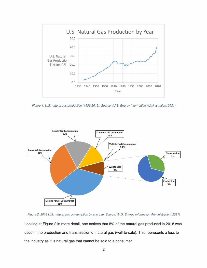
since 1967 as shown in Figure 1.

As the demand for affordable energy in the United States has increased, so has the production

and use of natural gas. Natural gas is commonly used as a heat source for power plants and

industrial processes as well as commercial and residential heating systems. A breakdown of

natural gas consumption in the United States in 2018 is shown below in Figure 2.

2

Figure 1: U.S. natural gas production (1936-2019). Source: (U.S. Energy Information Administration, 2021)

Figure 2: 2018 U.S. natural gas consumption by end use. Source: (U.S. Energy Information Administration, 2021)

Looking at Figure 2 in more detail, one notices that 8% of the natural gas produced in 2018 was

used in the production and transmission of natural gas (well-to-sale). This represents a loss to

the industry as it is natural gas that cannot be sold to a consumer.

0.0

10.0

20.0

30.0

40.0

50.0

1930 1940 1950 1960 1970 1980 1990 2000 2010 2020

U.S. Natural

Gas Production

[Trillion ft3]

Year

U.S. Natural Gas Production by Year

3

1.1 – Natural Gas Processing and Transmission

Natural gas, similar to other materials extracted from the earth, needs to be processed before it

is ready for use in power plants, residential hot water heaters, and furnaces among other things.

The processing of natural gas typically includes the removal of water, oil, and non-hydrocarbon

gases such as carbon dioxide and hydrogen sulfide. Some examples of what a natural gas

mixture may look like at the wellhead are shown in Table 1.

Table 1: Some typical natural gas compositions. Adapted from (Eser, n.d.)

Gas Canada Kansas Texas

methane (CH4) 77.1 73 65.8

ethane (C2H6) 6.6 6.3 3.8

propane (C3H8) 3.1 3.7 1.7

butane (C4H10) 2 1.4 0.8

pentane (C5H12) + 3 0.6 0.5

hydrogen sulfide (H2S) 3.3 0 0

carbon dioxide (CO2) 1.7 0 0

nitrogen (N2) 3.2 14.7 25.6

helium (He) 0 0.5 1.8

Additional cryogenic processing may occur to liquefy heavier hydrocarbons such as butane,

propane, and ethane for sale as other products (U.S. Energy Information Administration, 2021),

(Mokhatab, Poe, & Mak, 2015). The resulting gas mixture is mostly alkanes with the majority

molar fraction being methane with subsequently smaller fractions of heavier hydrocarbons. The

processed natural gas must meet strict specifications before it is ready for transportation in a

pipeline with typical “pipeline quality” specifications for natural gas shown in Table 2.

4

Table 2: Typical Pipeline Gas Specifications. Adapted from (Mokhatab, Poe, & Mak, 2015)

Characteristic Specification

Water content 4-7 lbm H2O/MMscf of gas

Hydrogen sulfide content 0.25-1.0 grain/100 scf

Gross heating value 950-1200 Btu/scf

Hydrocarbon dewpoint 14-40°F at specified pressure

Mercaptans content 0.25-1.0 grain/100 scf

Total sulfur content 0.5-20 grain/100 scf

Carbon dioxide content 2-4 mol%

Oxygen content 0.01 mol% (max)

Nitrogen content 4-5 mol%

Total inerts content (N2+CO2) 4-5 mol%

Sand, dust, gums, and free liquid None

Typical delivery temperature Ambient

Typical delivery pressure 400-1200 psig

Once the natural gas is processed to meet pipeline standards, it is ready for transmission. This

is critical as most natural gas wells and processing plants are far from end users. To transmit

the processed natural gas, vast networks of natural gas pipelines have been constructed across

the United States totaling 305,000 miles which connect over 11,000 delivery points (U.S. Energy

Information Administration, 2008). An overview of the interstate and intrastate pipelines in the

lower 48 can be seen in Figure 3. To ensure that the natural gas is continuously flowing

through the interstate and intrastate pipelines, over 1,400 compressor stations are used to

maintain the pipeline pressure as shown in Figure 4. Note that these are only the mainline

compressor stations and each compressor station typically has more than one compressor.

5

Figure 3: Inter/Intrastate pipelines in the lower 48. Source: (U.S. Energy Information Administration, 2009)

Figure 4: U.S. pipeline network compressors. Source: (U.S. Energy Information Administration, 2008)

6

One source estimated in 2018 that there are “approximately 1,700 midstream natural gas

pipeline compressor stations with a total of 5,000-7,000 compressors” (Brun, 2018). In addition

to this, the “US has approximately 13,000-15,000 smaller compressors in upstream and 2,000-

3,000 compressors (all sizes) in downstream oil & gas and LNG applications” (Brun, 2018). This

implies that there are somewhere between twenty to twenty-five thousand compressors in the

United States that continuously provide the pressures necessary to ensure that natural gas

makes the journey from the well head to the processing facilities, through the entire processing

facility, and eventually through the pipeline infrastructure to get the product to the customer.

Thus, compressors are integral to ensuring that natural gas is continuously flowing to provide

electricity and heat for the United States not to mention other countries.

1.2 – Reciprocating Gas Compressor Essentials

Although there are many different types of gas compressors, the focus of this thesis will be on

reciprocating compressors as they are ubiquitous in the natural gas industry. Reciprocating

compressors are a type of positive displacement compressor that employ a piston – cylinder

setup to increase the pressure of a gas by reducing the volume of the gas in an enclosed space.

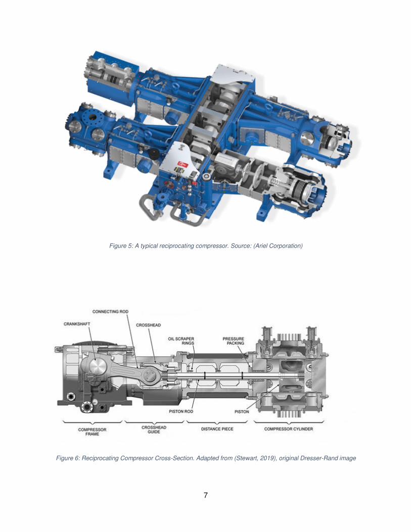
Figure 5 and Figure 6 show cutaway and cross-sectional views respectively of typical

reciprocating compressors.

7

Figure 5: A typical reciprocating compressor. Source: (Ariel Corporation)

Figure 6: Reciprocating Compressor Cross-Section. Adapted from (Stewart, 2019), original Dresser-Rand image

8

Referring to Figure 6 and working from left to right, natural gas engines or electric motors are

used to turn the compressor’s crankshaft. The power from the crankshaft is transmitted through

the connecting rod to the crosshead which is directly connected to the piston by the piston rod.

This causes the piston to cycle back and forth as the crankshaft revolves similar to an

automobile engine except that the power is transmitted in the opposite direction. For those

familiar with automobile engines, the horizontal orientation of these compressors is cause for

substituting the notion of Top-Dead-Center (TDC) and Bottom-Dead-Center (BDC) with Outer-

Dead-Center (ODC) and Inner-Dead-Center (IDC) respectively.

It is common for the moving parts of a machine to use a lubricant to ensure the parts do not

wear down during operation and reciprocating compressors are not exempt from this. Again,

referring to Figure 6, we will draw our attention to the oil scraper rings which can be found

between the crosshead guide and the distance piece. These rings ensure that any lubricant

escaping the moving parts to the left of the oil scraper rings are returned to the sump of the

compressor frame after use. This allows the lubricant in this part of the compressor to be pulled

from the frame sump and reused exactly how a lubricant is reused in an automobile engine with

regular oil changes, sampling, and level checks possible.

1.3 – Reciprocating Compressor Lubricants and Lube Rates

In contrast to the compressor frame and crosshead, the lubricant used in the rest of the

compressor cannot be reused. The lubricant injected into the pressure packing (or simply

“packing”) to prevent wear between the packing and the piston rod is lost to the distance piece

drain or the compressor cylinder. Similarly, lubricant is injected into the compressor cylinder to

prevent wear between the piston rings and the compressor cylinder wall but this lubricant is

eventually swept into the compressor discharge and carried away with the high-pressure gas

9

where it must be filtered out to meet the specifications shown in Table 2. These components are

shown in more detail in Figure 7 and Figure 8.

Figure 7: Detail of the piston-ring cylinder interface. Adapted from: (Ariel Corporation, n.d.)

Figure 8: A piston with six (smaller) piston rings and two (wider) rider bands. Source: (Burckhardt Compression, 2021)

The lubricant injected into the compressor cylinder is subjected to harsher conditions than in the

compressor frame and crosshead guide as it must prevent wear while subjected to a gas at high

temperatures and pressures.

10

1.3.1 - Lubricants

Lubricants are typically selected to have properties that meet the specific requirements of an

application. These typically include viscosity characteristics and chemical material compatibility

among other properties and lubricants used in reciprocating gas compressors are no different.

The lubricant used in these portions of the compressor must meet a viscosity standard but with

the added complication that gases at high pressures are can be absorbed into liquids. As the

high-pressure gas mixes into the lubricant, it reduces the lubricant’s viscosity. This

phenomenon, hereafter referred to as “dilution”, will be discussed in detail in later chapters.

Thus, the lubricants used in these areas of the compressor must meet their viscosity

requirements while resisting the chemical attack from the gas. These lubricants must also

prevent corrosion of the compressor cylinder as natural gas is often water saturated (Hanlon,

2001).

1.3.2 - Lube Rate

The compressor cylinder and packing see high gas pressures, requiring a force feed lubrication

pump to inject the lubricant into the cylinder and packing as a passive lubrication system would

not overcome the pressure. This injection of lubricant occurs at set intervals based on the

compressor’s operating speed and the settings on the force feed lubrication pump. The regular

injection of lubricant is known as the “lube rate” and can be varied by the operator of the

compressor.

At first pass, it may seem most reasonable to inject a large amount of lubricant that has a high

enough viscosity to withstand dilution from the gas. This would protect the compressor

components and prevent unnecessary wear or even failures. However, one must be wary of two

things: where the lubricant ends up and the price of the lubricant. Any lubricant injected into

these portions of the compressor must be removed from the high-pressure gas stream or the

11

distance piece drain and then disposed of properly. Thus, injecting excessive amounts of

lubricant has the potential to overload downstream gas filtration equipment in addition to

increasing disposal costs. On top of this, compressor lubricant prices range between $7 and

$50 per gallon (Yance, Justin; Hagan, Joe; Ariel Corporation, n.d.). This creates a significant,

up-front expense for a lubricant that may only lubricate the components for a matter of minutes

on its once-through use in the system. Here lies a tradeoff; lubricant must be injected into the

cylinder to prevent the piston rings and cylinder from wearing down. However, if too much

lubricant is injected into the cylinder, it can overload downstream filtration equipment causing a

shut down while wasting money. So, a compressor operator must balance the need to prevent

costly equipment failures with the need to prevent costly shutdowns for overloaded filtration

equipment. So, what do these costs look like to an operator?

1.4 – Natural Gas Compressor Lubrication and Maintenance Costs

The value of a natural gas compressor is relative to the amount of gas it pumps and the value of

that gas at that time. Thus, the natural gas compressor operator is most concerned with a

compressor’s up time as that provides value to their customer. To provide consistent

compressor operation, the operator knows the compressor must be properly lubricated to avoid

wearing down the moving parts prematurely. Yance & Hagan note that “[a] 1000 horsepower

compressor can consume 2,000 gallons of oil annually while larger compressors can approach

6,000 gallons annually” and lubricants can cost “$7 to $15 per gallon for mineral oils and $20 to

$50 per gallon for synthetic lubricants”. Assuming a compressor consumes 6,000 gallons of

lubricant annually, implies a lubricant cost anywhere from $42,000 to $300,000 annually per

compressor depending on the lubricant used. This sounds expensive but Yance & Hagan

estimate the costs associated with a compressor failure to be much higher as shown in Table 3.

12

Table 3: Expenses of equipment failures. Adapted from: (Yance, Justin; Hagan, Joe; Ariel Corporation, n.d.)

Expense Cost

Labor (overtime) $2000/day

Packing and piston ring replacement $3,000

Expedited shipping $4,000

Cylinder replacement $25,000

Lost production $40,000/day

Using these numbers, the cost-benefit analysis for the lubricant becomes apparent. The cost of

the lubricant for this compressor would at most total $300,000 annually if using a synthetic

lubricant at a premium of $50/gallon. However, this is far cheaper than failing a compressor as

even eight days of lost production for repairs would cost more than the annual cost of premium

lubricant. Thus, operators are inclined to err on the side of overlubricating their compressors to

prevent costly compressor failures, shutdowns, and repairs but in doing so may be missing out

on savings from reducing lubricant consumption and reduced processing needs downstream.

Given the criticality of the compressor lubricant, how can an operator select an effective

lubricant and lubrication rate for a specific compressor? The focus of this thesis will be to

identify and analyze the resources currently available to determine reciprocating compressor

lubricant and lubrication rate suggestions. In addition to this, an investigation of how the

thermophysical properties of a lubricant affect these suggestions will be presented. This will be

done by showing how the thermophysical properties of a lubricant can change when in contact

with a high-pressure gas environment as measured through a laboratory investigation as well as

a field study. Finally, a computer model of how the thermophysical properties of a lubricant

affect the lubricant flow under a piston ring will be discussed.

13

Chapter 2 – Previous work on Lubricant Dilution and Lubrication

Theory

2.1 - Current Lubricant and Lubrication Rate Suggestions

There are many resources available to an operator when selecting a lubricant and lube rate for

a reciprocating compressor including compressor handbooks, OEM manuals, and aftermarket

lubrication system manufacturers, among others. However, these resources can provide

drastically different suggestions due to the numerous factors that can affect the lubricant and

lube rate required for a specific compressor. As one source puts it, “No formula or graph can

cover all possible conditions, pressures, speeds, gases, and ring materials” (Hanlon, 2001).

Starting with this rather pessimistic conclusion, let us compare a few of these sources to see

how they match up.

2.1.1 - Compressor Handbook

In the “Compressor Handbook”, Hanlon (2001) provides the aforementioned quote on the state

of lubrication rates but also makes suggestions for how to select a lubricant for use in a

reciprocating compressor based on:

1. The “cold flow” temperature of the lubricant which is given as “6,000 to 10,000 SUS”

equivalent to 1295 to 2185 cSt.

2. The compressor discharge temperature.

3. The minimum oil viscosity noting “when lubricating oil reaches the viscosity equivalent to

water, the oil film no longer supports dynamic loads resulting in rapid failure. This

minimum viscosity is recognized as about 36 SUS” or 3cSt.

14

4. Gas absorption of the compressed gas into the lubricant.

5. Lubricant washing with liquid hydrocarbons.

6. Additives that may improve the lubricant’s performance for a specific application.

Moving on to lubrication rates, Hanlon (2001) presents the diagram shown in Figure 9 as a

graphical means to calculate the lubrication rate for a specific compressor.

Figure 9: "Oil Feed Rate" as presented by Hanlon (2001)

Upon investigation of this diagram, we see that it accounts for five things:

1. The compressor’s bore.

2. The compressor’s stroke.

15

3. The compressor’s speed.

4. The compressor’s discharge pressure.

5. The gas composition, piston ring material, and lubricant type/injection manner.

This appears to be a rather comprehensive treatment of lubricants and lubrication rates.

However, on the topic of lubricant gas dilution, it notes that the “gas dilution effect is hard to

accurately measure and/or predict without time-consuming laboratory tests using the actual gas

stream components elevated to the operating cylinder pressure and temperature.” Additionally,

the lube rate diagram allows for only three possible gas types including “Wet Field Gases”, “Wet

CO2”, and “Transmission Gases”. “Transmission Gases” can be roughly confined to a range of

gas compositions by the pipeline standards mentioned previously. However, the composition of

“Wet Field Gases” and “Wet CO2” can vary and the chart only provides a multiplication factor of

3.3 or 2.5 for each case, respectively. Since both factors would drastically increase the lubricant

consumption of the compressor, it would make sense to put some example gas compositions or

describe how these factors may vary for different gas compositions. For instance, “Wet CO2”

may contain water vapor at anywhere from 0-100 relative humidity (Tanneberger & Feldmann,

1983) and the main identifier for a “Wet Field Gas” is any composition with less than 85%

methane (Schlumberger, 2021). However, this still presents a lot of variability if the remaining

15% is mostly ethane versus a heavier hydrocarbon. This presents the issue with lubrication

rates – namely that they are based on extensive knowledge of the industry but are not an exact

science. This is further evidenced by Figure 10 where Hanlon (2001) present how the lifetime of

a piston ring or packing depends on an unscaled lube rate.

16

Figure 10: A comparison of packing and piston ring lifetime versus lube rate from (Hanlon, 2001)

2.1.2 - Ariel Corporation

Ariel Corporation is a reciprocating compressor manufacturer that provides guidance on

lubricants and lube rates for their customers. Reviewing Ariel’s publicly available documents

shows suggestions for lubricant selection as well as a trial-and-error method to determine

proper lubrication rates (Yance, Justin; Hagan, Joe; Ariel Corporation, n.d.). To guide lubricant

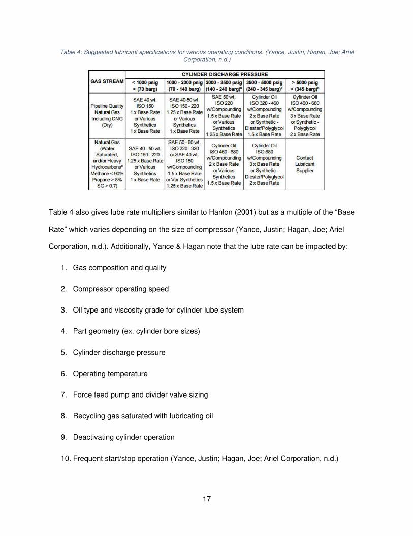
selection, the authors provide Table 4.

17

Table 4: Suggested lubricant specifications for various operating conditions. (Yance, Justin; Hagan, Joe; Ariel Corporation, n.d.)

Table 4 also gives lube rate multipliers similar to Hanlon (2001) but as a multiple of the “Base

Rate” which varies depending on the size of compressor (Yance, Justin; Hagan, Joe; Ariel

Corporation, n.d.). Additionally, Yance & Hagan note that the lube rate can be impacted by:

1. Gas composition and quality

2. Compressor operating speed

3. Oil type and viscosity grade for cylinder lube system

4. Part geometry (ex. cylinder bore sizes)

5. Cylinder discharge pressure

6. Operating temperature

7. Force feed pump and divider valve sizing

8. Recycling gas saturated with lubricating oil

9. Deactivating cylinder operation

10. Frequent start/stop operation (Yance, Justin; Hagan, Joe; Ariel Corporation, n.d.)

18

Due to the large variations in operating conditions these compressors may see, the authors

introduce what shall be referred to as the Cigarette Paper Test for the remainder of this thesis.

The Cigarette Paper Test is a trial-and-error method to determine proper lubrication rates and

Yance & Hagan describe the procedure as follows:

“This test estimates the amount of oil present on the cylinder bore by transferring oil from

the bore to thin layers of unwaxed cigarette paper. The paper test should be performed

within one hour of stopping the unit to get the best representation of cylinder oil film

during operation. The test is carried out by the following steps:

1. Using light pressure, wipe the cylinder bore with two layers of regular unwaxed

cigarette paper together. Begin at the top and wipe downward about 20°

(between 1/4” to 4-5/8” depending on bore size) along the bore circumference.

The paper against the bore surface should be stained (wetted with oil), but the

second paper should not be soaked through.

2. Repeat the test at both sides of the bore at about 90° from the top, using two

clean papers for each side. Paper against the bore surface not stained through

may indicate under-lubrication; both papers stained through may indicate over-

lubrication.”

For the reader’s reference, Yance & Hagan provide results from the Cigarette Paper Test that

indicate an overlubricated and a properly lubricated compressor cylinder as shown in Figure 11

and Figure 12, respectively.

19

Figure 11: Cigarette Paper Test Result - An indication of an overlubricated cylinder as presented in:

(Yance, Justin; Hagan, Joe; Ariel Corporation, n.d.)

Figure 12: Cigarette Paper Test Result - An indication of an “adequately lubricated cylinder"

(Yance, Justin; Hagan, Joe; Ariel Corporation, n.d.)

20

This Cigarette Paper Test is done in tandem with visual inspections of the lubricated

components as well as leak checking the packing. If the results of the Cigarette Paper Test

indicate an overlubricated cylinder, the lube rate is decreased by 10% and the compressor

operates for another month. Then the compressor is shut down and the Cigarette Paper Test

commences again with an overlubricated result leading to another 10% reduction in the lube

rate. This procedure is repeated until an “adequately lubricated” result is determined assuming

no components show visible or measurable signs of wear or leaking.

Though this information has proven itself in the field, it unfortunately is only possible to

determine during a compressor shut down. Thus, any changes in operating conditions could

affect whether the compressor is properly lubricated or not and the operator cannot afford to

shut down the compressor to verify proper cylinder lubrication every time operating conditions

change. In addition to this, another Ariel manual notes that “The paper test indicates only oil film

quantity. Aftermarket devices exist that measure flow. Neither method indicates viscosity quality.

Oils diluted with water, hydrocarbons, or other constituents may appear to produce an adequate

film or flow, but dilution will reduce lubricant effectiveness below requirements” (Ariel

Corporation, 2020). This indicates that the operator needs to know how the gas being

compressed will affect the viscosity of the lubricant in the compressor cylinder.

2.1.3 - Dresser-Rand (A Siemens Business)

Dresser-Rand, a part of Siemens AG since 2014 (Siemens, 2014), is also a reciprocating

compressor manufacturer. Reviewing some of their publicly available materials indicates that

lube rates and lubricant selection can be impacted by:

• The internal surface area of the compressor cylinder

• The compressor’s pressure

• The compressor’s speed

21

• The type of gas

• The compressor’s differential pressure

• The lubricant’s viscosity

• The compressor’s discharge temperature

• The lubricant’s chemical composition (Dresser-Rand (A Siemens Business), 2015)

They provide Table 5 to aid in the lubricant selection process.

Table 5: Siemens compressor cylinder lubricant selection table. Source: (Dresser-Rand (A Siemens Business), 2015)

For suggesting lubrication rates, three charts are provided which account for the compressor’s

diameter and discharge pressure, speed, and the density of the gas being compressed as

shown in Figure 13, Figure 14, and Figure 15 respectively.

22

Figure 13: Suggested lube rates for compressor break-in with water-saturated gas: (Dresser-Rand (A Siemens Business), 2015)

Figure 14: Dresser-Rand (Siemens) compressor speed correction factor: (Dresser-Rand (A Siemens Business), 2015)

23

Figure 15: Dresser-Rand (Siemens) gas density correction factor: (Dresser-Rand (A Siemens Business), 2015)

The specification mentions quite clearly “[t]his standard has been developed empirically and is

the result of input from several service and engineering sources” again indicating the use of

industrial experience. Additionally, the Cigarette Paper Test is presented in the same manner as

in Yance & Hagan but with a 5% suggested change in lube rates depending on the results of the

test in contrast to Ariel’s 10%. Similar to Ariel, the Dresser-Rand manual also gives the caveat

that the Cigarette Paper Test does not give an indication of the lubricant’s viscosity (Dresser-

Rand (A Siemens Business), 2015).

2.1.4 - Sloan Lubrication Systems

Sloan Lubrication Systems provides aftermarket lubrication systems for reciprocating

compressors (among other equipment) that claim significant reductions in lubricant consumption

when compared to OEM recommendations. In a conference paper presented at the 2018 Gas

Machinery Conference, Sloan claims an “over 90% reduction in compressor lubricant

24

consumption” (Sloan, 2018). The analysis presents Equation 1 as a method to determine

proper lubrication rates.

Equation 1

Of note is that this formula takes into account the compressor’s bore (B), stroke (S), and speed

(R) in addition to the denominator (X) which “varies depending on oil type/viscosity, cylinder

discharge pressure/temperature, and gas composition” (Sloan, 2018). Again, it is noted that the

selection of the denominator (X) for a specific application determined through “knowledge

gained through years of experience” (Sloan, 2018). Similar to the compressor manufacturers,

the Cigarette Paper Test is called out to determine proper cylinder lubrication with the caveat

that “Discharge pressure and temperature become factors because the hydrocarbon gases are

soluble in lubricants, decreasing the oil viscosity at elevated pressure and temperature” (Sloan,

2018).

In addition to these four sources, there are numerous other suggestions for selecting the proper

lubricant for a reciprocating compressor and interested parties can investigate the products

offered by any lubricant manufacturer in addition to other literature sources such as those by

Summers-Smith (1967) and even online resources (Scott, 2003).

2.1.5 - Comparison of the Four Sources

So, let us compare what these four sources would suggest for a compressor with an 8-inch

bore, an 8-inch stroke, running at 1000 rpm with pure methane at a discharge pressure of 1500

psia.

Hanlon suggests 1.4-2.8 pints/day assuming PTFE piston rings. Ariel suggests a base rate of

2.4-4 pints/day depending on the size of the compressor frame. Dresser-Rand/Siemens

25

suggests 10.8 pints/day as the break in rate with a reduction to “somewhere between 67% to

50% of the original "break-in" rates” after proceeding with the cigarette paper test. This implies a

final lube rate of 5.4-7.2 pints/day. Finally, using the formula from [Sloan] gives a suggested

lube rate of 2 pints/day assuming the value for the denominator (X) given in the paper holds for

this case.

This provides rather promising results for the operator of this compressor as the suggested lube

rates are on the same order of magnitude but may still vary by up to a factor of five. Thus,

determining and utilizing an optimum lubrication rate could result in significant savings.

2.1.6 - Overview of the Physical Phenomena Considered

All four sources produced similar values for the previous example compressor and account for

various operating conditions that can impact the required lubricant and lubrication rate. These

variations in operating conditions can be broadly grouped into two categories:

1. Compressor specifics. This includes the compressor’s bore, stroke, and operating

speed. Although accounted for in different manners, each source notes the obvious

correlation that increasing the compressor’s bore, stroke, and/or operating speed will

inherently require an increase in the lube rate. This physically correlates to the surface

area which must be properly lubricated and the rate at which the piston travels across

this surface. These correlations will not be addressed in detail in this thesis.

2. Lubricant properties. Again, each source accounts for this differently but empirically

recognizes the following physics that can affect the lubricant in the compressor cylinder:

i. The lubricant’s viscosity is important to preventing wear to the compressor’s

parts.

ii. The lubricant’s viscosity is affected by the compressor’s operating temperature.

This is due to the dependence of viscosity on temperature.

26

iii. The lubricant’s viscosity is affected by the composition of the gas and the

pressure of the gas in the compressor cylinder in two ways – dilution and

washing. Dilution refers to the reduction in a lubricant’s viscosity as it absorbs a

gas, while washing refers to the removal of lubricant from the cylinder wall due to

liquids in the gas stream. Dilution will be discussed in detail through the rest of

this thesis while washing will only be briefly mentioned.

2.2 - Fluid Viscosity

Three of the four previous sources note the importance of using the cigarette paper test to

ensure the compressor cylinders are properly lubricated. However, the cigarette paper test

comes with the complication that it does not account for reductions in the lubricant’s viscosity at

the compressor’s operating conditions. Let us first examine the concept of viscosity and the

implications it would have for a reciprocating compressor.

The viscosity of a fluid is defined by Merriam-Webster as: “the property of resistance to flow in

any material with fluid properties” or “the mathematical ratio of the tangential frictional force per

unit area to the velocity gradient perpendicular to the direction of flow of a liquid” (Merriam-

Webster, n.d.). The first definition provides the simplest description of a fluid’s resistance to

flow; implying that honey and water have different viscosities. The second definition would be

best appreciated in tandem with an illustration and we will begin a derivation of viscosity here

using Figure 16 as a reference.

27

Figure 16: A differential fluid element between two plates

Figure 16 depicts a volume of fluid between two plates separated by a distance 𝑑𝑧. The lower

plate is held stationary. The upper plate is then moved to the right at a constant speed

producing a linear velocity gradient in the fluid as shown in Figure 17.

Figure 17: The sheared fluid element after some differential time step (dt)

The shear on the fluid element is given by the angle 𝛾 which can be calculated as:

𝑠ℎ𝑒𝑎𝑟 = 𝛾 = tan−1 𝑑𝑥𝑑𝑧 Equation 2

28

Using the small angle approximation reduces this to:

𝑠ℎ𝑒𝑎𝑟 = 𝛾 = 𝑑𝑥𝑑𝑧 Equation 3

Using the velocity of the upper plate and the differential time step allows us to write:

𝑠ℎ𝑒𝑎𝑟 = 𝛾 = 𝑑𝑈𝑑𝑡𝑑𝑧 Equation 4

We then define the shear rate as the change in the shear with respect to time:

𝑠ℎ𝑒𝑎𝑟 𝑟𝑎𝑡𝑒 = �̇� = 𝑑𝑈 𝑑𝑡𝑑𝑧 𝑑𝑡 = 𝑑𝑈𝑑𝑧 Equation 5

Measuring the velocity of the upper plate and the separation distance between the two plates

allows for a calculation of the shear rate. Additionally, the force required to move the plate can

be measured to calculate the shear stress acting on the fluid. In rheology, fluids are subjected to

increasing shear stresses while the shear rate in the fluid is measured. This allows for a plot of

the shear stress versus the shear rate in the fluid as shown in Figure 18.

Figure 18: A comparison of fluids with different rheological properties

29

The relationship between the shear stress and the shear rate is termed the dynamic viscosity.

The dynamic viscosity is represented symbolically by the small, Greek letter mu or eta and is

defined as:

𝜇 = 𝜂 = 𝜏�̇� = [𝑀𝐿𝑇] Equation 6

The counterpart to the dynamic viscosity is the kinematic viscosity represented symbolically by

the small, Greek letter nu or eta and is defined as:

𝜐 = 𝜇𝜌 = [𝐿2𝑇 ] Equation 7

Substituting the shear rate from Equation 5 into Equation 6 and rearranging yields:

𝜏 = 𝜇 ( 𝑑𝑈𝑑𝑧) Equation 8

This fluid property indicates how a shear stress applied to a fluid will cause the fluid to shear.

Figure 18, depicts a Newtonian fluid (e.g. water, normal alkanes) in comparison to a shear-

thickening fluid (e.g. cornstarch and water) and a shear thinning fluid (e.g. paint). A Newtonian

fluid is defined as having a linear relationship between the shear stress and shear rate.

However, the viscosity can also be dependent on the shear stress in the case of shear-

thickening and shear-thinning fluids.

In addition to these descriptions of viscosity, anyone familiar with fluids such as honey or syrups

would point out that the viscosities of these fluids are highly temperature dependent. In fact,

viscosity is a function of both the temperature and pressure of a fluid (Spectris, PLC, 2016).

From this derivation one notes that a higher viscosity results in less deformation of a fluid

element but what does this imply for a reciprocating natural gas compressor?

30

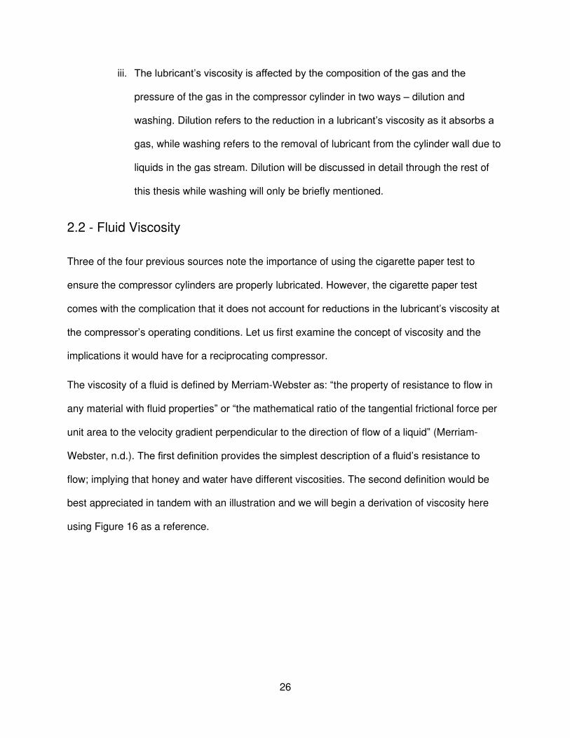
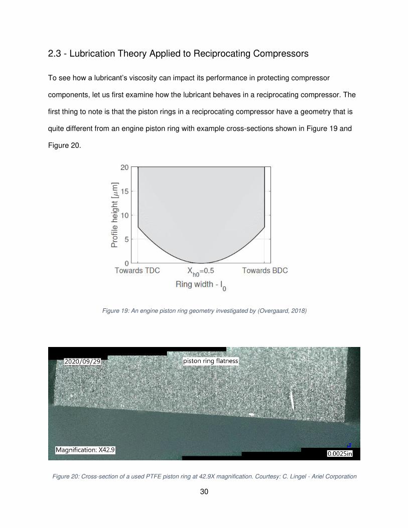
2.3 - Lubrication Theory Applied to Reciprocating Compressors

To see how a lubricant’s viscosity can impact its performance in protecting compressor

components, let us first examine how the lubricant behaves in a reciprocating compressor. The

first thing to note is that the piston rings in a reciprocating compressor have a geometry that is

quite different from an engine piston ring with example cross-sections shown in Figure 19 and

Figure 20.

Figure 19: An engine piston ring geometry investigated by (Overgaard, 2018)

Figure 20: Cross-section of a used PTFE piston ring at 42.9X magnification. Courtesy: C. Lingel - Ariel Corporation

31

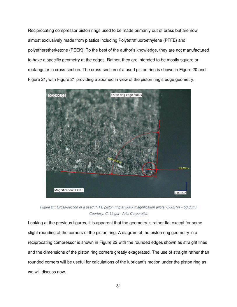
Reciprocating compressor piston rings used to be made primarily out of brass but are now

almost exclusively made from plastics including Polytetrafluoroethylene (PTFE) and

polyetheretherketone (PEEK). To the best of the author’s knowledge, they are not manufactured

to have a specific geometry at the edges. Rather, they are intended to be mostly square or

rectangular in cross-section. The cross-section of a used piston ring is shown in Figure 20 and

Figure 21, with Figure 21 providing a zoomed in view of the piston ring’s edge geometry.

Figure 21: Cross-section of a used PTFE piston ring at 300X magnification (Note: 0.0021in = 53.3µm).

Courtesy: C. Lingel - Ariel Corporation

Looking at the previous figures, it is apparent that the geometry is rather flat except for some

slight rounding at the corners of the piston ring. A diagram of the piston ring geometry in a

reciprocating compressor is shown in Figure 22 with the rounded edges shown as straight lines

and the dimensions of the piston ring corners greatly exagerated. The use of straight rather than

rounded corners will be useful for calculations of the lubricant’s motion under the piston ring as

we will discuss now.

32

Figure 22: Cross-sectional view of a PTFE piston ring in a reciprocating compressor

Lubrication theory is a section of fluid dynamics where the viscous and pressure forces

dominate the flow. In these situations, the Navier-Stokes equations can be condensed into

another form known as the Reynold’s equation. Here we will begin our investigation with the

integrated incompressible, iso-viscous, steady-state form of Reynold’s equation given as:

𝑑𝑃𝑑𝑥 = 6𝜇𝑈 ℎ − ℎ𝑚ℎ3 − 𝑤ℎ𝑒𝑟𝑒 − 𝑑𝑃𝑑𝑥|ℎ=ℎ𝑚 = 0

Equation 9

Where 𝑃 represents the pressure, 𝑥 represents the direction parallel to the piston ring’s motion, 𝜇 represents the lubricant’s dynamic viscosity, 𝑈 represents the speed of the piston ring, ℎ

represents the separation between the compressor cylinder and the piston ring, and ℎ𝑚

33

represents the film thickness where the first derivative of pressure with respect to 𝑥 is zero. The

piston ring geometry is shown in more detail in Figure 23 with the x-axis representing the

compressor cylinder.

Figure 23: Piston ring geometry for use in derivations

2.3.1 - Converging Section

Looking closely at Figure 23, one notices that the left side of the piston ring will be subjected to

the same physics as a fixed-inclined slider with only some slight differences on the boundary

conditions as shown in Figure 24.

34

Figure 24: Comparison of the canonical slipper pad problem and the current situation.

Investigating Figure 24 in more detail shows that with a few change in variables, the canonical

fixed-incline slider bearing can be converted to the left hand side of the piston ring currently

under investigation. Aside from the variable changes, there is also a change of the boundary

conditions. The canonical situation assumes the inlet and outlet gas pressures are equal to

atmospheric pressure while our situation assumes only the inlet gas pressure is known. This

presents an added difficulty that will be addressed shortly.

We now follow the canonical solution for the fixed-incline slider as presented by Hamrock,

Schmid, and Jacobson (2004) with some slight changes. First, the geometry of the inclined

slider is defined as:

ℎ = ℎ0 + 𝑠ℎ (1 − 𝑥𝑙)

Equation 10

35

Equation 9 and Equation 10 are often nondimensionalized as demonstrated Hamrock, Schmid,

and Jacobson (2004) using:

�̅� = 𝑃𝑠ℎ2𝜇𝑈𝑙 𝐻 = ℎ𝑠ℎ 𝐻𝑚 = ℎ𝑚𝑠ℎ 𝐻0 = ℎ0𝑠ℎ 𝑋 = 𝑥𝑙

Equation 11

Which produces:

𝑑�̅�𝑑𝑥 = 6 (𝐻 − 𝐻𝑚𝐻3 ) Equation 12

𝐻 = 𝐻0 + 1 − 𝑋

Equation 13

𝑑𝐻𝑑𝑋 = −1

Equation 14

Integrating Equation 12 yields:

�̅� = 6 (1𝐻 − 𝐻𝑚2𝐻2) + �̅� Equation 15

This leaves one equation with two unknowns; 𝐻𝑚 which is the nondimensionalized film

thickness where the first derivative of pressure with respect to 𝑥 is zero and an integration

constant �̅�. Now, the canonical solution calls for the application of the following boundary

conditions:

36

�̅� = 0 𝑤ℎ𝑒𝑛 𝑋 = 0 𝑜𝑟 𝐻 = 𝐻0 + 1 Equation 16

�̅� = 0 𝑤ℎ𝑒𝑛 𝑋 = 1 𝑜𝑟 𝐻 = 𝐻0 Equation 17

This is where our path must diverge from the canonical solution as we do not have the same

boundary conditions. We have a similar pressure boundary condition at the inlet allowing us to

write:

�̅� = �̅�1,𝑔𝑎𝑠 𝑤ℎ𝑒𝑛 𝑋 = 0 𝑜𝑟 𝐻 = 𝐻0 + 1 Equation 18

However, now we must come up with another boundary condition. For the right boundary

condition, the pressure is unknown. However, upon inspection of Figure 23, we can say one

thing about the pressure at this location: it must be a maximum. This is evident from a

knowledge of flows between parallel, flat plates as the flat portion of the piston ring cannot build

up any pressure. Similarly, the sloped section on the right side of the piston ring cannot build up

any pressure. This allows us to return to Equation 9 and say that we now know the value of ℎ𝑚

must be equivalent to the height at the outlet (ℎ0) which allows us to write:

ℎ𝑚 = ℎ0 → 𝐻𝑚 = 𝐻0 Equation 19

Substituting Equation 18 and Equation 19 into Equation 15 yields:

�̅�1,𝑔𝑎𝑠 = 6( 1𝐻0 + 1 − 𝐻02(𝐻0 + 1)2) + �̅� Equation 20

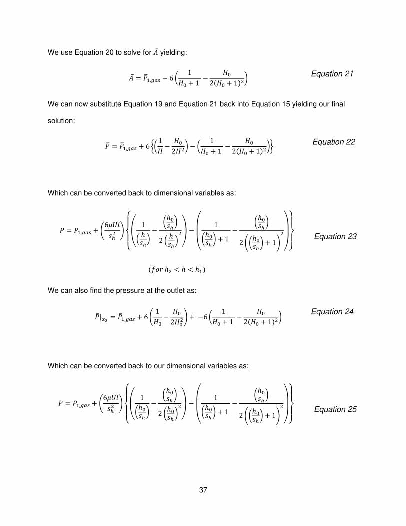
37

We use Equation 20 to solve for �̅� yielding:

�̅� = �̅�1,𝑔𝑎𝑠 − 6( 1𝐻0 + 1 − 𝐻02(𝐻0 + 1)2) Equation 21

We can now substitute Equation 19 and Equation 21 back into Equation 15 yielding our final

solution:

�̅� = �̅�1,𝑔𝑎𝑠 + 6 {(1𝐻 − 𝐻02𝐻2) − ( 1𝐻0 + 1 − 𝐻02(𝐻0 + 1)2)} Equation 22

Which can be converted back to dimensional variables as:

𝑃 = 𝑃1,𝑔𝑎𝑠 + (6𝜇𝑈𝑙𝑠ℎ2 ){ ( 1( ℎ𝑠ℎ) −

(ℎ0𝑠ℎ)2 ( ℎ𝑠ℎ)2) −( 1(ℎ0𝑠ℎ) + 1 −

(ℎ0𝑠ℎ)2((ℎ0𝑠ℎ) + 1)2) }

(𝑓𝑜𝑟 ℎ2 < ℎ < ℎ1)

Equation 23

We can also find the pressure at the outlet as:

�̅�|𝑥3 = �̅�1,𝑔𝑎𝑠 + 6( 1𝐻0 − 𝐻02𝐻02)+ −6( 1𝐻0 + 1 − 𝐻02(𝐻0 + 1)2) Equation 24

Which can be converted back to our dimensional variables as:

𝑃 = 𝑃1,𝑔𝑎𝑠 + (6𝜇𝑈𝑙𝑠ℎ2 ){ ( 1(ℎ0𝑠ℎ) −

(ℎ0𝑠ℎ)2 (ℎ0𝑠ℎ)2) −( 1(ℎ0𝑠ℎ) + 1 −

(ℎ0𝑠ℎ)2((ℎ0𝑠ℎ) + 1)2) }

Equation 25

38

From here a variable substitution can convert between the solution for the fixed-incline slider or

the piston ring entrance as shown in Figure 24.

2.3.2 - Diverging Section

For the diverging section on the right hand side of the piston ring in Figure 24, we note that the

slope is the opposite from the previously investigated section. We will again begin with the

integrated incompressible, iso-viscous, steady-state form of Reynold’s equation given as:

𝑑𝑃𝑑𝑥 = 6𝜇𝑈 ℎ − ℎ𝑚ℎ3 − 𝑤ℎ𝑒𝑟𝑒 − 𝑑𝑃𝑑𝑥|ℎ=ℎ𝑚 = 0 Equation 26

Again, we do not have the pressure at the point where the flat portion of the ring meets the

sloped section (𝑥3). However, here we will assume the Reynold’s or Gümbel’s boundary

condition at the right-most side of the piston ring (𝑥4). Reynold’s or Gümbel’s boundary

condition states that the fluid pressure gradually turns into the outlet pressure which is

mathematically given by:

𝑃|𝑥=𝑥4 = 𝑃2,𝑔𝑎𝑠 − 𝑎𝑛𝑑 − 𝛿𝑃𝛿𝑥|𝑥=𝑥4 = 0 Equation 27

This allows us to write:

ℎ𝑚 = ℎ4 → 𝑑𝑃𝑑𝑥|ℎ=ℎ4 = 6𝜇𝑈 ℎ4 − ℎ4ℎ3 = 0 Equation 28

∴ 𝑑𝑃𝑑𝑥 = 6𝜇𝑈 ℎ − ℎ4ℎ3 Equation 29

39

Similar to the method proposed by (Kruse, 1974), we calculate the slope of the diverging section (𝑚2) as:

𝑚2 = 𝑑ℎ𝑑𝑥 (𝑓𝑜𝑟 𝑥3 < 𝑥 < 𝑥4) = ℎ4 − ℎ3𝑥4 − 𝑥3

Equation 30

Separating variables and substituting Equation 30 into Equation 29 yields:

𝑑𝑃 = 6𝜇𝑈 ℎ − ℎ4ℎ3 𝑑𝑥 = 6𝜇𝑈𝑚2 (ℎ − ℎ4ℎ3 )𝑑ℎ Equation 31

Integrating across the diverging region allows us to write with our known pressure as the

boundary condition:

∫ 𝑑𝑃𝑃2,𝑔𝑎𝑠𝑃 = 6𝜇𝑈𝑚2 ∫ (ℎ−2 − ℎ4ℎ−3)𝑑ℎℎ4ℎ Equation 32

Which simplifies to:

𝑃 = 𝑃2,𝑔𝑎𝑠 + (6𝜇𝑈𝑚2 ) [ ℎ42ℎ2 − 1ℎ + 12ℎ4] (𝑓𝑜𝑟 ℎ3 < ℎ < ℎ4)

Equation 33

2.3.3 - Parallel Section

Between Equation 23 and Equation 33 we can now find the pressures at the edges of the flat

portion of the piston ring (𝑥2 and 𝑥3) using only the pressures on either side of the piston ring

and the piston ring geometry. Now the center section of the piston ring that is parallel to the

40

compressor cylinder is the only section left to evaluate. Using the same assumptions as for the

previous equations, the flow under this section of the piston ring can be described simply as a

flow between two parallel flat plates with a constant pressure drop. This gives the pressure drop

under the flat portion of the ring as:

𝑑𝑃𝑑𝑥 = 𝑃|𝑥=𝑥3 − 𝑃|𝑥=𝑥2𝑥3 − 𝑥2

Equation 34

Which can be integrated to yield:

𝑃 = 𝑃|𝑥=𝑥3 − 𝑃|𝑥=𝑥2𝑥3 − 𝑥2 (𝑥 − 𝑥2) + 𝑃|𝑥=𝑥2 (𝑓𝑜𝑟 𝑥2 < 𝑥 < 𝑥3)

Equation 35

Additionally, the flow rate and fluid velocity through this portion of the piston ring are given by

Hamrock, Schmid, and Jacobson (2004) as:

𝑞′ = − ℎ312𝜇 𝑑𝑃𝑑𝑥 + 𝑈ℎ2 (𝑓𝑜𝑟 𝑥2 < 𝑥 < 𝑥3)

Equation 36

𝑢 = 12𝜇 𝑑𝑃𝑑𝑥 (𝑦2 − 𝑦ℎ) + 𝑈𝑦ℎ (𝑓𝑜𝑟 0 ≤ 𝑦 ≤ ℎ)

Equation 37

From here, we will use Newton’s Postulate to find the frictional force per unit length for the flat

section of the piston ring. Where Newton’s Postulate is given as:

𝑓 = 𝜇𝐴𝑈ℎ Equation 38

41

The pressure difference in this portion of the piston ring forces causes the fluid velocity to lose

linearity thus requiring integration across the gap between the piston ring and the compressor

cylinder as:

𝑓 = 𝜇𝐴𝑈ℎ = 𝜇𝐴 𝑑𝑢𝑑𝑦

Equation 39

Substituting the derivative of Equation 37 yields:

𝑓 = 𝜇𝐴 ( 12𝜇 𝑑𝑃𝑑𝑥 (2𝑦 − ℎ) + 𝑈ℎ)

Equation 40

From here, we note that the area (𝐴) the friction force acts on is the bottom edge of the piston

ring multiplied by the circumference of the piston ring. Since we are doing this for a one-

dimensional cross-section, we remove the piston ring’s circumference to make the friction force

per unit length and evaluate the remaining equation at (𝑦 = ℎ) yielding:

𝑓′ = (𝑥3 − 𝑥2) (ℎ2 𝑑𝑃𝑑𝑥 + 𝜇𝑈ℎ )

Equation 41

Now we have the frictional force acting on a majority of the piston ring’s area (Equation 40) in

addition to the lubricant flowrate under the piston ring (Equation 36) and the hydrodynamic

pressure generated under the piston ring (Equation 23, Equation 33, and Equation 35). This

provides a sufficient starting point with which to model a compressor piston ring as detailed in

Chapter 5 – Modeling Compressor Lubrication. However, let us first make note of the

importance of viscosity in the equations above and its influence on compressor lubrication.

42

1. Increasing the lubricant’s viscosity increases the hydrodynamic force built up under the

piston ring (see Equation 23 and Equation 33). This increases the separation gap (ℎ) between the piston ring and the compressor cylinder to prevent wear.

2. Increasing the lubricant’s viscosity increases the frictional force acting against the piston

rings’ motion (see Equation 41).

3. Increasing the lubricant’s viscosity has counteracting effects on the lubricant flowrate

under the piston ring (see Equation 36). Increasing the lubricant’s viscosity increased the

value in the denominator of Equation 36 but also increases the separation gap (ℎ) between the piston ring and the compressor cylinder.

Reviewing the equations in relation to an operating compressor, it is evident that the

compressor operator cannot vary the geometry of the piston rings and typically does not want to

vary the compressor’s speed. Thus, the lubricant viscosity and lube rate are the only

parameters the operator has control over. Contemplating the equations governing the

hydrodynamic pressure (Equation 23, Equation 33, and Equation 35), one will note that once

the lubricant’s viscosity is too low, there is no amount of lubricant that can be supplied to keep

proper separation between the cylinder wall and the piston ring. Thus, higher viscosity lubricants

are typically suggested for harsher operating conditions as can be seen by investigating Table 4

and Table 5. There are many more sources besides the ones previously mentioned to aid an

operator in selecting the correct lubricant for a certain application. However, how can an

operator be sure these suggestions are correct for their specific application?

2.4 - Lubricant Viscosity and Gas Dilution Estimation

The lubricant viscosity and lubrication rate are the only controls an operator has to protect their

operating compressor. There are many suggestions for proper lubricants and lubrication rates

but how can the operator know these suggestions are correct for their specific application? Is

43

there a way to measure or calculate the viscosity of the lubricant in the compressor? The high

temperatures and pressures in a compressor preclude the use of many types of sensors that

could measure the lubricant’s viscosity in-situ. This leaves calculations or laboratory

measurements. Addressing the first, the lubricant’s viscosity will depend on the compressor’s

temperature which the operator can estimate to be somewhere between the compressor’s

suction and discharge temperatures. However, the temperature will not provide the whole

picture as the high-pressure gases in the compressor are soluble in liquids (including lubricants)

which can cause the lubricant to be diluted with the gas in the cylinder. So, the operator needs a

way to estimate the amount of a gas that will dissolve into a lubricant and, using the amount of

dissolved gas, estimate the viscosity of the lubricant in the compressor. Unfortunately, there is

still one limitation to this method described nicely by Seeton (2009):

“Given the nature and diversity of lubricants, there are no reliable prediction models

to estimate the solubility of liquefied gases in lubricants across the broad spectrum

of lubricant types and blends. Lubricating oils are generally made-up of a blend of

basestock fluids to reach a desired viscosity, viscosity index and lubricity for the final

product. This blending makes it possible to efficiently tailor products for different

applications; however, blending also makes it difficult to generalize the solubility of

gases into these blends within the same manufactures product line, and across

different manufactures of the same type classification. Therefore, solubility data must

be experimentally measured for specific combinations of interest to have accurate

information for the system of interest” (p 36).

So, it appears that the operator is stuck relying on recommendations from the lubricant

manufacturer or needs to experimentally measure the viscosity of multiple lubricants when

subjected to their specific natural gas stream to see what is best for their specific application.

The focus of this thesis is on the experimental determination of a lubricant’s viscosity when

44

diluted with natural gas components. Before addressing this though, let us first discuss the

solubility data that does exist for similar gas-lubricant systems and ways to estimate how the

dissolved gas will affect the viscosity of the lubricant.

2.4.1 - Gas Solubility in Lubricants

The topic of gas solubility in liquids was of great interest to early chemists in the 1800s. As

such, many measurements were taken with various instruments to determine the amount of gas

dissolved in certain solvents but the range of measurement techniques unfortunately ended in

many different systems for denoting the solubility as discussed in (Markham & Kobe, 1941) ,

(Battino & Clever, 1966), and (Battino R. , 1984). ASTM standard D2779 addresses these

issues by providing conversions between the many different types of solubility definitions

including Henry’s Law constants, Ostwald Coefficients, and Bunsen Coefficients. ASTM

standard D2779 also provides estimates of the solubility of gases in petroleum liquids with a

density around 0.85g/mL and ASTM standard D3827 provides solubility estimates of gases in

petroleum. Both standards note that “gas solubility is of extreme importance in the lubrication of

gas compressors” (ASTM International, 2020). These standards do not cover all gases that may

be found in natural gas but do include methane, hydrogen sulfide, carbon dioxide, nitrogen, and

hydrogen. These calculations allow for predictions of gas solubility in lubricants at the elevated

temperatures and pressures seen in natural gas compressors. However, one must be wary of

the assumptions used in these calculations – namely the use of Henry’s Law at elevated

pressures where the gas solubility may not be linearly dependent on the partial pressure of the

gas. An additional limitation is that both standards focus on hydrocarbon-based lubricants and

thus may not provide accurate solubility estimates for polyolester (POE), polyalphaolefin (PAO),

or polyalkylene glycol (PAG) lubricants.

Given the potential for errors in extrapolating these calculations to higher pressures or different

gas-lubricant combinations, a literature review of experimental solubility data was conducted for

45

systems of natural gas components in lubricant solvents. The previous research can be broadly

categorized into two groups: oilfield and refrigeration. Beginning with oilfield applications, the

determination of the solubility of gases in liquids is important for processes such as enhanced

oil recovery (EOR), drilling rig “gas kick”, and developing equations of state (EOS) to describe

crude mixtures. Articles focusing on EOR were not evaluated in this paper as they typically

focus more on carbon dioxide and nitrogen solubility in crude and these gases are minority mole

components in natural gas. Table 6 documents studies from the oilfield that provide data

relevant to this thesis.

Looking at the sources listed in Table 6, it is evident that extensive research on the solubility of

gases in a range of hydrocarbon liquids was conducted in the 1930s. Though many of these

sources give a great starting point for examining solubility values, they often use archaic

solvents including “gas oil”, “crystal oil”, and “spray oils”. Additionally, the compositions of these

solvents are not stated and, in one case, even the composition of the “dry natural gas” was not

stated (Lacey, Sage, & Kircher, Jr., 1934). The last four studies listed in Table 6 are more

recent investigations that provide the compositions of both the gases and lubricants used in

their experiments.

46

Table 6: Table of relevant studies on the solubility of gases in lubricants from the oil and gas industry

Gas(es) Relevant

Solvent(s)

Temperature

°F (°C)

Pressure

psia (bara)

Reference

methane, nitrogen,

propane, hydrogen

sulfide

"Gas Oil" 77(25) 2939 (202.7) (Frolich, Tauch,

Hogan, & Peer, 1931)

dry natural gas Crude 100, 200 (38, 93) 3000* (207.9) (Lacey, Sage, &

Kircher, Jr., 1934)

propane "Crystal

Oil", Crude

70-200 (21-93) 300* (21.7) (Sage, Lacey, &

Schaafsma, 1934)

methane, propane "Spray Oil",

Crude

86-140 (30-60) 3000* (207.9) (Hill, 1934)

ethane "Crystal Oil" 70-220 (21-104) 3000 (207.9) (Sage, Davies,

Sherborne, & Lacey,

1936)

methane, ethane,

nitrogen, carbon

dioxide, natural gas

Mentor 28

Base Oil

100-300 (38-149) 3000 (207.9) (O'bryan, 1988)

methane Diesel oil,

mineral oil,

olefin oil,

ester oil

194 (90) 5076 (350) (Berthezene,

Hemptinne, Audibert,

& Argillier, 1999)

methane Alkanes,

esters

158,194 (70,90) 10153 (700) (Ribeiro, Pessôa-

Filho, Lomba, &

J.Bonet, 2006)

methane White oil,

PAO

158 (70) 4351 (300) (Feng, Fu, Chen, Du,

& Qin, 2016)

*Pressures are not explicitly stated to be absolute or gauge pressures in article

47

In addition to the oil and gas industry, the solubility of refrigerant gases in lubricants is a

common research topic for the refrigeration industry. Though this may at first pass seem distant

from the focus of this thesis, propane (R290), butane (R600), and isobutane (R600a) have been

investigated as refrigerants and thus efforts have been made to evaluate the solubility of these

gases in a range of lubricants as detailed in Table 7.

Table 7:Table of relevant studies on the solubility of gases in lubricants from the refrigeration industry

Gas(es) Relevant

Solvent(s)

Temperatures

°F (°C)

Pressures

psia (bara)

Reference

R-290 (propane)

R-600a (isobutane)

Mineral Oil

&

Synthetic *

86-212

(30-100)*

*

(Spauschus, Henderson,

& Grasshoff, 1994)

R-600a (isobutane) MO 86-194 (30-90) 247 (17) (Zhelezny, Zhelezny,

Procenko, & Ancherbak,

2007)

R600a (isobutane) POE 50-140 (10-60) 131 (9) (Neto & Barbosa, Jr.,

2008)

R-290 (propane)

MO 3-129 (-16-54) 276 (19) (Wu, Chen, Lin, & Li,

2018)

R-290 (propane) POE 50-176(10-80) 326 (22.5) (Czubinski, Sanchez,

Silva, Neto, & Barbosa,

Jr., 2020)

R-290 (propane)

MO -4-158(-20-70) 168 (11.6) (Wang, Jia, & Wang,

2021)

*Unable to find reference article, information obtained from (Neto & Barbosa, Jr., 2008)

Of note in Table 7 is that the pressures are much lower than would be seen in a natural gas

compressor but the partial pressure of propane or butane in natural gas should be well below

48

these values for most applications. Additionally, propane and butane are typically only minor

components in the natural gas stream. (Spauschus & Henderson, 1990) note that propane and

isobutane can reduce a lubricant’s viscosity but give measures of apparent miscibility rather

than solubility or viscosity.

Thus, there is an assortment of solubility data for most of the components of natural gas in

various lubricants as discussed above with some online resources even addressing the topic

(G.E. Totten & R. J. Bishop, 2002). Assuming these solubility measurements could be

generalized, the next task is to determine the effect a dissolved gas will have on the viscosity of

the lubricant into which it is dissolved.

2.4.2 - Viscosity Prediction of Gas-Lubricant Mixtures

The importance of estimating the viscosity of a mixture is apparent for our purpose but also for

other processes in the oil and gas and refrigeration industries as mentioned previously. Seeton

(2009) does a comprehensive literature review for this topic and points to the use of ASTM

standard D7152 combined with ASTM standard D341 for a method to estimate the viscosity of a

mixture. In this method though, it is noted that ASTM standard D341 fails for chemicals with a

viscosity under 0.21cSt which is common for gases at high temperatures and thus an improved

equation for linearizing the viscosity is presented which allows for continued used of the

blending method provided in ASTM standard D7152 (Seeton C. J., 2009). In addition to this,

Seeton (2009) also notes the dearth of experimental viscosity data for supercritical gases and

suggests using the viscosity of the gas at the critical point as an effective estimate of the

supercritical gas viscosity. As the review presented by Seeton (2009) was extensive, we shall

move on from this topic.

At this point, we have shown that there is experimental data on the solubility of gases in some

lubricants and there are methods for estimating how the gas dissolved in a lubricant will affect

49

its viscosity. However, for the case of a specific natural gas blend in a specific lubricant, one

would have to assume some manner of mixture parameters based on the composition of the

gas and the lubricant and, as mentioned previously, the composition of a lubricant is often not

known by anyone aside from the lubricant manufacturer and the composition can change

depending on the base stocks used. As such, many generalizations and assumptions would

have to be made to calculate a final viscosity estimate which often reduces the usefulness of

such calculations and thus experimental methods are typically employed to determine the

viscosity of a specific lubricant when saturated with a specific natural gas species or blend.

In this area, research has been rather sparse. In addition to the work of Sage, Lacey, and

Schaafsma (1934), Swearingen and Redding (1942) present some of the first measurements of

a lubricant’s viscosity at high gas pressures and temperatures. They published the viscosity of

various lubricants when diluted with a specified natural gas mixture at pressure up to 3500 psig

(242 bara) at temperatures up to 86°C (186°F). Again, the composition of the lubricants is not

provided presenting the complication of using these results for other lubricants. Matthews

(1987) presents two viscosity data points: one for an ISO 680 mineral oil and one for a 200 cSt

PAG both saturated with methane at 340 bar and 100°C as part of a small paragraph on this

topic. As data in this area was rather sparse and archaic, recent work measured the viscosity,

density, and solubility of multiple lubricants currently used in natural gas compressors when

diluted with methane, ethane, propane, butane, and pentane (Seeton C. J., 2019). This work

presented excellent equilibrium viscosity data for the industry with industrially relevant lubricants

and single gas components. However, two questions remained: (1) how long would it take for a

lubricant to reach equilibrium with a natural gas species or mixture in a compressor and (2) how

would a natural gas mixture affect the viscosity of a lubricant as compared to a single natural

gas species?

50

2.5 - Dilution rate and Gas Mixtures

The challenges affecting the previous sections also hold true for these topics. Diffusion rates

have been measured for many gas-liquid combinations to give estimates of the rate at which a

gas and liquid will mix. Research mentioned previously measured the rate of solution of

methane and propane into “spray oil” and various samples of crude (Hill, 1934). Again though,

these measurements are specific to the gas-liquid combination and the composition of the liquid

is not well defined. Additionally, mixing rules and diffusion coefficients for alkane mixtures have

been investigated in depth but determining how these apply to a lubricant with an unknown

composition implies that physical measurements would be better than the use of theoretical

calculations. On top of all this, the lubricant film thickness through which the gas would diffuse in

a reciprocating compressor has never been published. Research is currently underway on this

topic and interested parties should inquire with the Gas Machinery Research Council (GMRC). It

is assumed that these films would be rather thin – on the order of tens of micrometers. This

precludes the use of the infinite dilution assumption commonly employed in diffusion

calculations while simultaneously not presenting a specific value for the diffusion length.

In light of all these complications with calculations, this work sets about to investigate two topics:

1) the rate at which a natural gas species or mixture dilutes or mixes with a specific

lubricant and how this may apply to various film thicknesses in a reciprocating

compressor

2) how a natural gas mixture may produce a different equilibrium viscosity than calculated

by ideal mixture assumptions coupled with the previously mentioned experimental data

from Seeton (2019).

Three studies were undertaken to address these topics. The first was a laboratory study to

measure the rate at which a gas mixed with (or diluted) a lubricant. The second focused on

51

gathering used oil samples from the field and determining the composition of the gas absorbed

by the lubricant to see if it matched ideal mixing assumptions. The third study was to model the

lubricant flow under a reciprocating compressor ring to give an estimate of the lubricant film

thickness and identify how variations in lubricant viscosity would affect the lubricant film

thickness and lubrication rates. We will discuss these in the order stated.

52

Chapter 3 – Lubricant Absorption of Natural Gas – Results from

the Laboratory

3.1 - Examining Prior Work

Before beginning the experimental work for this study, the work of Seeton (2009) was

investigated in detail. The experimental apparatus described therein presented an excellent

starting point for measuring the viscosity of a lubricant at high temperatures and pressures

when diluted with a gas. However, the experimental apparatus sprayed lubricant through a

volume of gas to quickly absorb the gas and obtain equilibrium. While this allowed for a

determination of a lubricant’s diluted viscosity in just a few minutes, it presented the potential to

incur errors related to the lubricant’s properties and spray pattern (surface tension, viscosity,

droplet size, distribution, etc.) when applied to the purposes of this study. In order to avoid these

complications and mimic how a gas and lubricant interact in a reciprocating compressor, it was

determined that slowly circulating a measured amount of lubricant in a loop while the lubricant

was exposed to a gas stream would provide a highly controlled vapor-liquid interface.

In addition to this, Seeton (2019) measured the properties of lubricants that were diluted with a

single natural gas component. Natural gas mixtures were not evaluated in that study as the

experimental apparatus began each test with a constant charge of lubricant and gas evaluated

on a mass fraction basis. This prevented the used of gas mixtures in the experiment as the

lubricant could preferentially absorb certain components of the gas mixture (e.g. pentane,

butane) which posed the potential to significantly change the composition of the gas in the

experiment. Thus, an open system that allowed gas to flow in and out of the experimental

53

apparatus was designed so the lubricant would be exposed to as much gas as necessary to

obtain equilibrium with each component in a gas mixture.

3.2 - Experimental Setup

Beginning with these considerations, a system was designed to allow a gas and lubricant to mix

through a vapor-liquid interface while measuring the viscosity of the liquid phase over time to

observe the difference between the initial “neat” viscosity and the final “diluted” viscosity of the

lubricant at a specific temperature and pressure. The viscosity was chosen as the measure of

how long it takes a gas to dilute a lubricant as it is the basis of many of the specifications. To

measure the lubricant viscosity at conditions relevant to operating compressors, components

were selected to withstand temperatures up to 150°C (302°F) and pressures up to 86.2 bara

(1250 psia). A schematic of the experiment is shown in Figure 25.

Figure 25: experimental setup to dilute a lubricant with gas. Gas flows from left to right as shown by the blue arrows, oil circulates clockwise with the red arrows shown. Components: 1. 3-way valve, 2. Pressure relief valve, 3. Inlet

throttling valve, 4. System pressure probe, 5. Gas-liquid interaction chamber, 6. Liquid gear pump, 7. Liquid sampling/drain valve, 8. Oscillating piston viscometer, 9. Outlet throttling valve, 10. Gas flow meter

54

The experimental apparatus circulates lubricant in a clockwise fashion around the loop indicated

by the red arrows in Figure 25. The lubricant is continuously recirculated through the experiment

such that it will eventually attain equilibrium with the gas stream allowing for equilibrium

properties to be measured at the end of the test. To maintain a constant flow of gas to the

experiment, the gas travels out of the interaction zone and is replaced by new gas as indicated

by the blue arrows in Figure 25. The gas and lubricant mix in the gas-liquid interaction zone

labeled as component 5 in Figure 25. In this zone, the gas and lubricant flow counter to one

another with an idealization shown in Figure 26.

Figure 26: a diagram of the gas-lubricant interaction zone in the experiment

The liquid and gas flowrates in the interaction tube were maintained as slow as possible to

produce laminar flows with the liquid Reynold’s number never exceeding 200 and the gas

Reynold’s number never exceeding 800. This provided a controlled interaction between the two

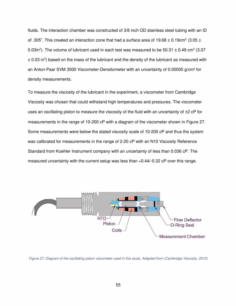
55

fluids. The interaction chamber was constructed of 3/8 inch OD stainless steel tubing with an ID

of .305”. This created an interaction zone that had a surface area of 19.68 ± 0.19cm2 (3.05 ±

0.03in2). The volume of lubricant used in each test was measured to be 50.31 ± 0.49 cm3 (3.07

± 0.03 in3) based on the mass of the lubricant and the density of the lubricant as measured with

an Anton-Paar SVM 3000 Viscometer-Densitometer with an uncertainty of 0.00005 g/cm³ for

density measurements.

To measure the viscosity of the lubricant in the experiment, a viscometer from Cambridge

Viscosity was chosen that could withstand high temperatures and pressures. The viscometer

uses an oscillating piston to measure the viscosity of the fluid with an uncertainty of ±2 cP for

measurements in the range of 10-200 cP with a diagram of the viscometer shown in Figure 27.

Some measurements were below the stated viscosity scale of 10-200 cP and thus the system

was calibrated for measurements in the range of 2-20 cP with an N10 Viscosity Reference

Standard from Koehler Instrument company with an uncertainty of less than 0.036 cP. The

measured uncertainty with the current setup was less than +0.44/-0.32 cP over this range.

Figure 27: Diagram of the oscillating piston viscometer used in this study. Adapted from (Cambridge Viscosity, 2012)

56

The temperature in the experimental apparatus was measured using a Pt100 Resistance

Temperature Detector (RTD) installed in the base of the Cambridge Viscosity viscometer as

shown in Figure 27. The RTD has an accuracy of ±0.15°C for the range of 0-200°C (32-392°F).

A PX119 Series Pressure Transducer from Omega Engineering with a range of 0-103.4 bara (0-

1500 psia) and an accuracy of ±0.52 bara (±7.5 psia) measured the pressure in the experiment.

The gear pump used to circulate the lubricant through the experiment was a GAH series from

Micropump capable of withstanding pressures up to 344.7 bara (5000psia) and temperatures

between -46 to 177°C (-50 to 350°F). The flowrate of lubricant through the experiment was

calculated using the data given from the manufacturer for the specific gears used (0.042 ml/rev

or 0.01 gal/1000*rev) and the revolutions were measured with the tachometer output signal from

the pump motor. As noted above, the liquid Reynold’s number was calculated to be well below

200 for every test ensuring laminar flow conditions.

The flowrate of gas through the experiment was measured using a GFC mass flow controller

from Aalborg capable of measuring gas flowrates from 0-1000mL/minute (0-61in3/min) with an

accuracy of ±6 mL/min from 0-200mL/minute and ±15 mL/min from 200-1000mL/minute. The

GFC mass flow controller can withstand pressures up to 68.9 bara (1000psia) but was installed

downstream of the outlet throttling valve so testing at higher pressures could be carried out. The

gas flowing through gas flowmeter was assumed to be at atmospheric pressure (roughly 0.84

bara or 12.2 psia at the laboratory location) and room temperature (between 16 and 27°C or 60

and 80°F depending on the season). The gas flow meter relies on a thermal gradient created in

the moving gas and thus varies depending on the specific heat and density of the gas flowing

through the meter. The ambient pressure and temperature along with the specific heat and

density of each gas were used to correct the measurements for each experiment. The low-

pressure flowrate measurements were used to calculate the high-pressure gas velocity for each

57

experiment to ensure the flow was laminar. As noted above, the gas Reynold’s number was

calculated to be well below 800 for every test ensuring laminar flow conditions.

Multiple lubricants were used during the course of this thesis with data collected for Mobil DTE

Extra Heavy, Mobil Pegasus 805 Ultra, Mobil Teresstic 150, PROGILINE® LPG-WS-150 from

Shrieve Chemical, and BT22 Biosynthetic® Base Oil from Biosynthetic Technologies. This

thesis will focus on the results for Mobil Pegasus 805 Ultra. All lubricants were used as

delivered from the supplier.

As the viscosity is highly dependent on the mixture composition, great care was taken to clean

the experimental apparatus after each test. The cleaning procedure began by draining the gas-

lubricant mixture from the experiment. After this, the system was flushed with hexane followed

by acetone until the hexane and acetone drained from the experiment had no signs of dissolved

lubricant. The system was then purged with gaseous nitrogen with a purity of 99.999% to

remove any residual hexane or acetone. Finally, the system was evacuated below 0.04 bara

(0.6 psia) to remove any residual vapors.

3.3 - Experimental Data Analysis

As this work focused on measuring how a gas reduced a lubricant’s viscosity at different

temperatures and pressures, some analysis was necessary to remove the impact that pressure

and temperature could have on the viscosity to allow for comparisons at different pressures and

temperatures.

3.3.1 - Pressure

Early testing noted that pressure had a non-negligible impact on the lubricant’s viscosity. As this

presented a potential source of error when measuring how quickly the lubricant viscosity

decreased, the system was originally filled with the required amount of lubricant and then

58

pressurized with gaseous nitrogen to the desired pressure. The lubricant was then allowed to

obtain equilibrium with the gaseous nitrogen before the gas flowing through the experiment was

switched over to the test gas. Though this initially proved fruitful, ASTM standard D2779-

92(2020) was consulted and it was noted that nitrogen solubility was on the same order of

magnitude as methane solubility for the temperature range under consideration as shown in

Figure 28.

Figure 28: Chart of Ostwald Coefficients at varying temperatures. Adapted from ASTM D2779-92(2020). Red box shows temperature range investigated

This meant that rather than mixing the test gas with a lubricant at high pressure, the test gas

was being mixed with a solution of lubricant and gaseous nitrogen. It was determined that this

procedure was not desirable as the test gas took many hours to equilibrate with the lubricant-

59

gaseous nitrogen mixture while taking less than one-half hour to equilibrate the test gas with the

lubricant when no nitrogen precursor was used. Thus, the nitrogen in the experiment was

affecting how the dilution process occurred and made conditions dissimilar to what would be

seen in the field. The nitrogen precursor was abandoned after for further testing.

As it was still of interest to determine the relationship between viscosity and pressure, the

primary lubricant studied in this work (Mobil Pegasus 805 Ultra) was pressurized with nitrogen

without the gear pump circulating the lubricant. This prevented the nitrogen from fully mixing

with the lubricant and allowed for a determination of the impact of the pressure on the lubricant’s

viscosity. The lubricant was then depressurized to ensure that there were no residual effects

from the nitrogen left in the lubricant. The lubricant’s viscosity was measured as the pressure

increased and decreased. Small variations in temperature were accounted for to discern the

pressure effects on viscosity. These tests were completed at temperatures of 50, 100, and

150°C and pressures up to 86.2 bara. Coefficients were determined at each temperature for the

Barus equation which is given by:

𝜇 = 𝜇0𝑒𝛼𝑃

Equation

42

Where 𝜇0 is the viscosity at atmospheric pressure and 𝛼 represents the pressure-viscosity

coefficient (Barus, 1893). Use of the Barus equation allowed for the pressure dependency to be

effectively removed allowing for comparisons of dilution data collected at different pressures

with a comparison of the measured and fitted viscosity data shown in Figure 29, Figure 30, and

Figure 31.

60

Figure 29: Estimated and measured viscosity-pressure dependence at 50°C for Mobil Pegasus 805 Ultra


61


Table 8: Coefficients determined for the Barus equation at 50°C, 100°C, and 150°C

Temperature

[°C]

Pressure-Viscosity Coefficient (α)

[bara-1]

50 0.0024

100 0.0019

150 0.0017

The coefficients shown in Table 8 were used to fit the data shown in Figure 29, Figure 30, and

Figure 31. The pressure-viscosity coefficients have the same order of magnitude as those

measured for other lubricants (van Leeuwen, 2009) and were used to account for pressure

fluctuations in the primary lubricant studied in this work (Mobil Pegasus 805 Ultra). The study of

the dependence of viscosity on pressure is typically of interest for extreme pressures seen in

62

bearing contacts. The coefficients shown in Table 8 indicate that the pressures in this

experiment can increase the viscosity by up to 23%.

3.3.2 - Temperature

While pressure can affect the lubricant’s viscosity as shown previously, it pales in comparison to

a lubricant’s temperature dependency as the viscosity can change by up to two orders of

magnitude over a range of 100°C (212°F). The viscosity’s dependence on temperature is

indicated by a Viscosity Index (VI) which can be calculated using ASTM D2270-10(2016). To

mitigate the effects of temperature, each test was conducted at a constant temperature ±1°C for

the duration of the test. However, it was of interest to compare dilution data at different

temperatures. Thus, each dilution data set was linearly scaled with the neat viscosity at that

temperature equal to unity (or 100%) and the diluted viscosity equal to zero (or 0%) after the

pressure effects were removed. The application of the pressure effect removal and temperature

scaling applied to a typical data point is shown below in Figure 32, Figure 33, and Figure 34.

Figure 32: A typical data set showing the decrease in a lubricant's viscosity as a gas (natural gas) is absorbed

63

Figure 33: An example of the removal of the pressure effects on the lubricant's viscosity

Figure 34: A typical data point scaled after the removal of the pressure effects.

64

Figure 34 shows the same viscosity data as Figure 33 but scaled to remove the effects of

temperature and pressure. Applying this scaling procedure allows for a comparison of data

points collected a different temperatures and pressures.

3.4 - Dilution Rates and Implications for Compressors

Testing was conducted with a natural gas mixture and the Mobil Pegasus 805 Ultra lubricant.

The molar composition of the natural gas was determined using a gas chromatography flame

ionization detector (GC-FID). As the GC-FID method only measures combustible gas species,

the composition was double checked with a gas chromatography thermal conductivity detector

(GC-TCD) which showed the amounts of nitrogen and carbon dioxide in the mixture. The gas

composition determined by both methods is shown in Table 9.

Table 9: Natural gas molar composition determined through GC-FID and GC-TCD analysis

Component

Molar Composition [%]

(GC-FID)

Molar Composition [%]

(GC-TCD)

methane 86.46 84.42

ethane 11.12 10.86

propane 2.05 2.00

butanes 0.34 0.33

pentanes 0.03 0.03

hexanes <0.01 0.013

carbon dioxide - 1.85

nitrogen - 0.5

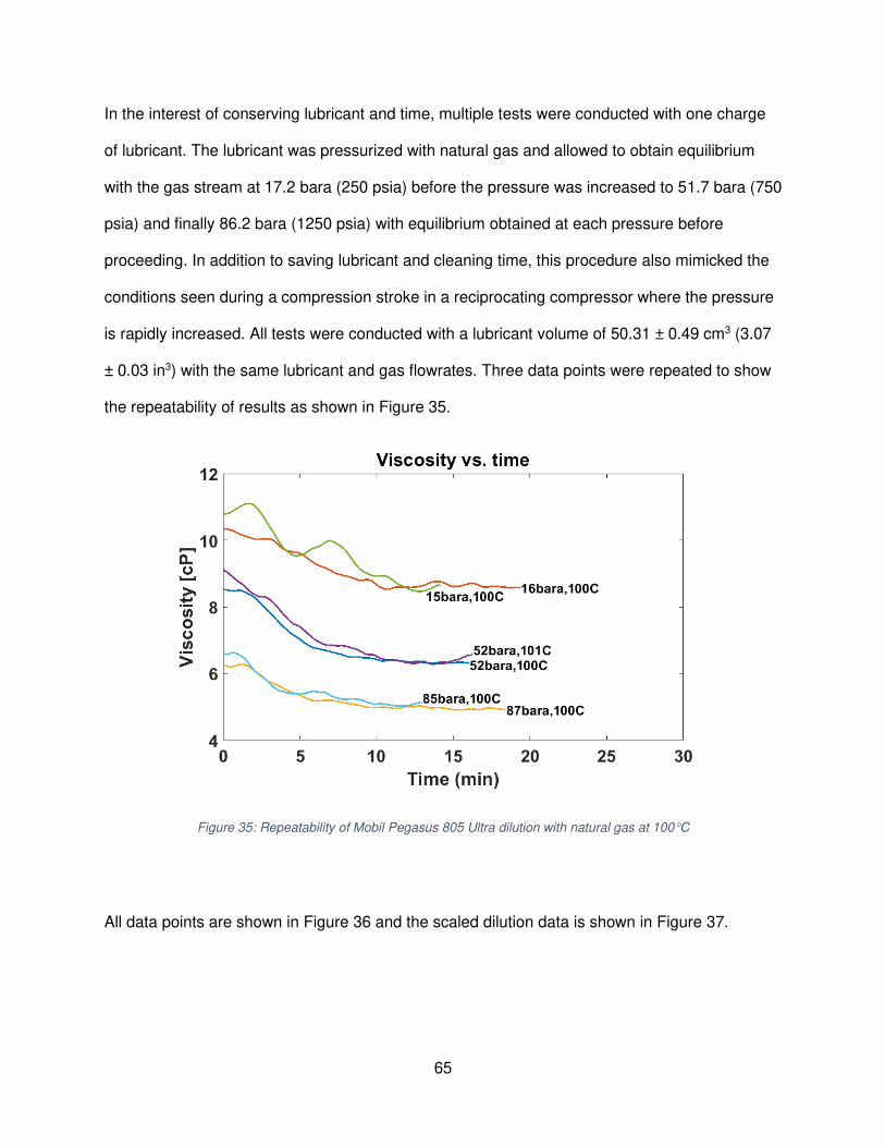
65

In the interest of conserving lubricant and time, multiple tests were conducted with one charge

of lubricant. The lubricant was pressurized with natural gas and allowed to obtain equilibrium

with the gas stream at 17.2 bara (250 psia) before the pressure was increased to 51.7 bara (750

psia) and finally 86.2 bara (1250 psia) with equilibrium obtained at each pressure before

proceeding. In addition to saving lubricant and cleaning time, this procedure also mimicked the

conditions seen during a compression stroke in a reciprocating compressor where the pressure

is rapidly increased. All tests were conducted with a lubricant volume of 50.31 ± 0.49 cm3 (3.07

± 0.03 in3) with the same lubricant and gas flowrates. Three data points were repeated to show

the repeatability of results as shown in Figure 35.

Figure 35: Repeatability of Mobil Pegasus 805 Ultra dilution with natural gas at 100°C

All data points are shown in Figure 36 and the scaled dilution data is shown in Figure 37.

66

Figure 36: Mobil Pegasus 805 Ultra dilution with natural gas at various temperatures and pressures

Figure 37: Scaled dilution data for various temperatures and pressures

67

Figure 37 shows that all test points reach full dilution between 10.7 and 23.7 minutes after

pressurization. The data does not provide any evidence of how variations in temperature or

pressure may affect the dilution rate due to the small sample size. However, an analysis of the

overall time to reach maximum dilution will still prove advantageous.

The experimental apparatus described in section 3.2 - Experimental Setup, though intended to

mimic the conditions inside a reciprocating compressor, is inherently not an actual reciprocating

compressor. One of the most apparent differences is the sheer size and dimensions of a

reciprocating compressor compared to the experimental apparatus. The volume of lubricant and

surface area through which the gas and lubricant interact in the experiment is compared to a

compressor cylinder with an 8-inch bore and an 8-inch stroke in Figure 38.

Figure 38: Comparison of the volume and gas-liquid interaction area in the experimental apparatus and a compressor

68

The large difference in scales between the experiment and a reciprocating compressor indicates

a difference of scale when applying the results from the experiment to a compressor.

Investigating Figure 38 shows that a typical compressor would have a gas-liquid interaction area

roughly 66 times larger than that in the experiment. Similarly, the volume of lubricant in the

compressor would at most equal the volume in the experiment assuming a lubricant film

thickness ten times larger than any film experimentally measured (Fatjo, Smith, & Sherrington,

2018). Both factors imply that the lubricant in a reciprocating compressor will be diluted much

faster than in the experiment described here.

The time to reach full dilution ranged from 10.7 to 23.7 minutes with an average of 15.7 minutes

in the experiment. Assuming a linear relation with the surface area would imply that a

reciprocating compressor with a surface area 66 times larger than the experiment and the same

volume of lubricant would have its lubricant fully diluted in 9.7-21.5 seconds. Looking at this

another way, we return to the lube rate calculations from section 2.1.5 - Comparison of the Four

Sources. This indicated a lube rate of 1.4 to 10.8 pints per day for this size of compressor which

equates to 28-213 cm3 of lubricant injected into the compressor cylinder every hour. Modifying

the experiment to hold a larger volume with the same surface area would theoretically allow a

volume of 127-282 cm3 of lubricant to be fully diluted in one hour.

Scaling up the experimental results based solely on the geometric scale of the experiment and a

compressor provides best-case scenarios as the experiment used a very slow, laminar flow of

gas at a constant pressure and temperature as well as a laminar flow of lubricant. This is in

contrast to a reciprocating compressor that has a highly turbulent gas stream, fluctuating

pressures, and convection in the lubricant due to thermal gradients or piston ring motion which

will all aid in diluting the lubricant with the natural gas. Due to these factors left unaccounted for,

the author highly suspects that the lubricant in an operating compressor is diluted much faster

than the estimates given above if not instantaneously.

69

If these claims have yet to convince the reader that the lubricant is fully diluted in the

compressor cylinder, let us investigate this question from an economic perspective. Yance &

Hagan indicate that costs related to compressor failure far outweigh the annual cost of even an

expensive lubricant. Thus, if data exists that a lubricant diluted with a gas fails to meet the

viscosity requirements of the compressor, operators should select a better lubricant in the

interest of reliability. Attempting to use a lubricant that does not meet the viscosity requirements

of the compressor when diluted with the process gas presents the potential to rapidly wear the

compressor components which makes a cheaper lubricant less cost effective.

With these factors in mind, what are the implications for lubricants and lube rates? As

mentioned above, the lubricants are estimated to absorb components of the process gas quickly

when used in an operating compressor. This implies that lubricant manufacturers and

compressor operators should be aware of their lubricant’s viscosity when mixed with the

process gas at the pressures and temperatures typically seen in each specific compressor.

Previous work (Seeton C. J., 2019) could serve as a valid starting point for the lubricants in that

study. Following we investigate the efficacy of applying those data and methods to a

multicomponent gas mixture and other lubricants. As for lubrication rates, this study implies that

lubricants are rapidly diluted in reciprocating compressors which implies that injecting extra

lubricant into a cylinder may not be as beneficial as injecting a lubricant with the best properties

for that specific application.

3.5 - Viscosity - Comparison with Previous Work

In addition to monitoring the rate at which the natural gas was absorbed, the equilibrium

viscosity of the mixture was measured at the end of each test. As mentioned previously, the

work of Seeton (2019) was completed for single gas components mixed with a lubricant. Thus,

to compare the results of this study with the results of Seeton (2019) requires some assumption

70

of how the mixture will behave. Ideal mixing based on Dalton’s law of partial pressures and the

mass fractions provided by Seeton (2019) was assumed allowing for a direct comparison. A

comparison of the results of this study and the predictions based on the data from Seeton

(2019) are presented in Figure 39, Figure 40, and Figure 41.

Figure 39: Comparison of measured and calculated viscosities for a natural gas- Pegasus 805 Ultra mixture at 100°C


71


Three tests were conducted at similar temperatures (100.6+1.3/-0.7°C) and pressures

(51.7±0.3 bara) to determine the repeatability of the results. The expected variation of the

diluted viscosity was ±0.1cP from the calculations at the different conditions but a variation of

±0.5cP was seen in the measurements. All measurements were less than 20cP and the

expected variation in this range was +0.44/-0.32cP based on calibration with a standard test

fluid. As the variation seen was outside of the expected range based on the calibration, error

bars of ±0.5cP were applied to all measurements. The maximum variation between the

measured and calculated viscosity was 1.04cP. It is noted that in eight out of nine tests, the

measured viscosity is higher than the predicted viscosity. Although the predicted viscosities are

outside of the error bounds of the measurements, they are still within 1.04cP and typically

predict a lower viscosity than was measured. Thus, the predicted viscosity based on ideal

mixing rules and the data from (Seeton C. J., 2019) serves as a good estimate of the viscosity a

lubricant diluted with a natural gas mixture for temperatures from 100-150C and pressures up to

72

87 bara with minimal differences observed. As the predicted values are slightly lower than the

measured values, the prediction method provides if nothing else, a margin of safety when

compared to the measured viscosity.

73

Chapter 4 – Lubricant Absorption of Natural Gas – Results from

the Field

4.1 - Purpose of Field Study

As mentioned previously, the work of Seeton (2019) did not investigate natural gas mixtures

over concerns that the lubricant would preferentially absorb certain parts of the gas mixture

which could not be replenished in the system. Thus, a field study was undertaken to collect

samples of used lubricant from the field that had seen a constant stream of natural gas.

Samples of used lubricant and natural gas were collected from a vapor recovery unit (VRU) in

Weld County, Colorado approximately forty miles from Colorado State University’s Powerhouse

Energy Campus. The compressors identified for sampling were two-stage, four-throw Ariel

compressors running Mobil Pegasus 805 Ultra as the lubricant. The first stage suction pressure

ranged from 24.9 to 27.2 bara (346 to 380 psig). The second stage discharge pressure ranged

from 78.2 to 81.0 bara (1120 to 1160 psig) with the discharge gas temperature varying from 93

to 116°C (200 to 240°F). Sample collection for this project was unique in that the samples had

to be collected under pressure. A pressure decrease would result in the lubricant releasing the

dissolved gases similar to how a carbonated beverage fizzes upon the container’s opening. To

capture the high-pressure gas or lubricant, thirteen sampling cylinders were constructed using a

piece of 3/8” OD tubing and two Swagelok needle valves. The sample bottles have a volume of

3.05±0.11 mL (0.1±0.004 ounces) which was determined through gravimetric analysis. Two

examples of the sampling cylinders in use are shown in Figure 42 below.

74

Figure 42: Sample bottles on a discharge bottle (left) and the discharge manifold (right)

4.2 - Locations and Lessons Learned

The industry partner identified for this project installed equipment allowing for sampling of the

inlet gas stream as well as the used lubricant. Multiple visits were made between January and

June 2020 to obtain samples and identify optimal sampling points. The goal was to find sample

locations close to the compressor to ensure that the pressure and temperature matched the

compressor’s operating conditions, but where sufficient amounts of used lubricant would drop

out of the gas stream and collect. The inlet gas stream was sampled upstream of the inlet

scrubber as shown in Figure 43.

Figure 43: Inlet Gas Sampling Point (upstream of compressor scrubber)

75

To obtain samples of used lubricant, it was imperative to sample from a low point drain near the

compressor discharge to ensure the temperature and pressure closely matched the conditions

seen in the compressor. Three sampling points were identified: 1) the low point drain on each

compressor discharge bottle, 2) a low point drain downstream from the second-stage discharge

manifold, and 3) a low point drain on the coalescing filter liquid discharge line. The discharge

bottles were initially suspected to be the best spot to collect used lubricant due to their proximity

to the compressors. Sampling valves were installed in the discharge bottle drain plugs as shown

in Figure 44.

Figure 44: Discharge bottle sampling point

When the sampling valves were initially installed, the drain plugs had very little lubricant on

them as seen in Figure 45. Initial samples pulled from this location were comprised of mainly

gas with a small amount of lubricant. Even after nearly five months of continuous operation, an

insufficient amount of oil had collected at this location to fully fill the small sample bottles used.

This was unfortunate as this location’s pressure and temperature were as close to the

compressor’s conditions as possible without retrofitting the compressor. The conditions at this

sampling location flucated between site visits with the pressure ranging from 78.2 to 81.0 bara

(1120 to 1160 psig) and the temperature ranging from 93 to 121°C (200 to 250°F).

76

Figure 45: Traces of used lubricant on discharge bottle drain plugs

Moving downstream from the compressor discharge bottles, the discharge gas (and used

lubricant) from each compressor flows into a single, central manifold. Directly after this manifold,

a low point drain was located with a sufficient amount of liquid for analysis as seen in Figure 46.

Figure 46: Compressor discharge manifold low point drain (under insulation)

The gas conditions at this sampling location flucated between site visits with the pressure

ranging from 79.2 to 80.4 (1134 to 1152 psig) and the temperature ranging from 104 to 116°C

(220 to 240°F). The author noted that although the sample point was under insulation and the

conditions in the pipe were known, this sampling location was exposed to the ambient

conditions. Thus, the temperature of the sampling point was documented on each visit ranging

between 27 and 60°C (80 and 140°F).

Moving further downstream, the natural gas and used lubricant travel through a cooler and then

through a coalescing filter. A large amount of the lubricant is removed in the coalescing filter

77

which must be periodically drained to prevent the buildup of liquids. A sampling point with a

sufficient amount of liquids was identified on the coalescing filter drain as seen in Figure 47.

Figure 47: Coalescing filter (left) and coalescing filter drain sampling point (right)

The gas conditions at this sampling location flucated between site visits with the pressure

ranging from 78.2 to 80.3 bara (1120 to 1150 psig) and the temperature ranging from 31 to 38°C

(87 and 100°F). Similar to the previous sampling point, the research team noted that this

sampling location was also exposed to the ambient conditions. Thus, the temperature of the

sampling point was documented on each visit ranging between 7.8 to 27°C (46 and 80°F) due

to the large temperature variations between the seasons.

4.3 - Sample Analysis

Samples gathered from the locations mentioned above, whether filled with used lubricant or the

compressor inlet gas, were taken back to the lab for analysis. As mentioned previously, any

decrease in the sample’s pressure would result in a release of the dissolved gas. To take

advantage of this, an apparatus capable of capturing the gas upon depressurization was

designed and built. A schematic of the system is shown in Figure 48.

78

Figure 48: Sample degassing apparatus

The analysis of the pressurized samples begins with connecting the oil containing sample

cylinder to the bottom of the expansion tank. The system is then evacuated below 0.002 bara

(0.024 psia) before the sample is depressurized into the enclosed, low pressure environment.

This converts a high-pressure gas sample into a low-pressure sample or allows gas entrained in

a lubricant sample to escape. The pressure in the system is monitored until the pressure obtains

a constant value. At this point, a portion of the gas in the expansion tank is extracted and

analyzed using a gas chromatograph (GC). The degassing system is then cleaned to remove

any residual gas or lubricant in preparation for the next test.

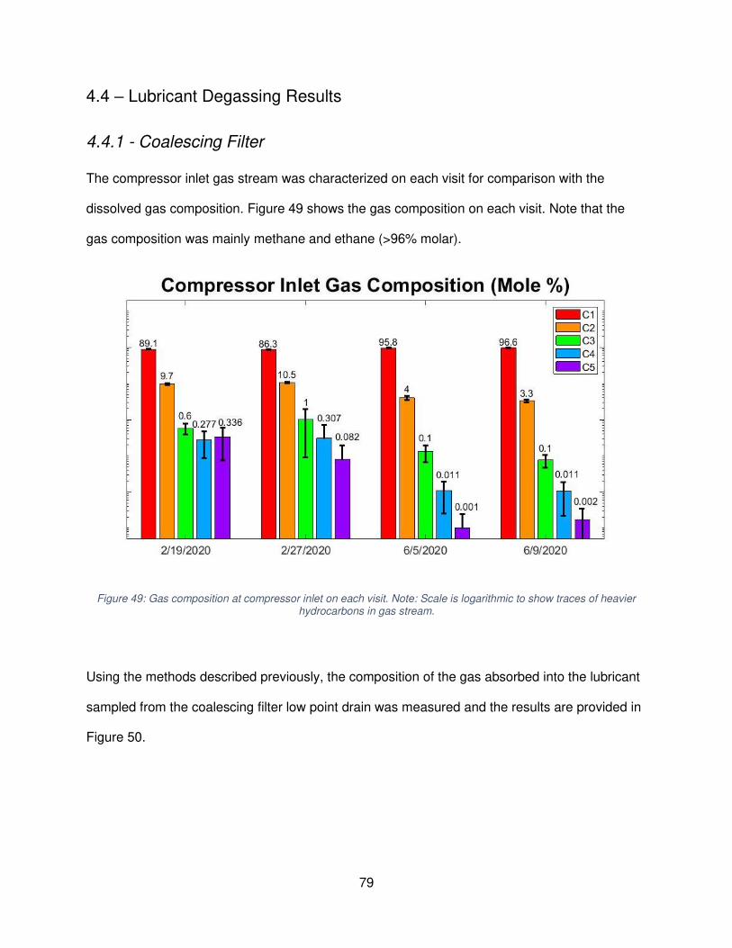
79

4.4 – Lubricant Degassing Results

4.4.1 - Coalescing Filter

The compressor inlet gas stream was characterized on each visit for comparison with the

dissolved gas composition. Figure 49 shows the gas composition on each visit. Note that the

gas composition was mainly methane and ethane (>96% molar).

Figure 49: Gas composition at compressor inlet on each visit. Note: Scale is logarithmic to show traces of heavier hydrocarbons in gas stream.

Using the methods described previously, the composition of the gas absorbed into the lubricant

sampled from the coalescing filter low point drain was measured and the results are provided in

Figure 50.

80

Figure 50: Composition of gas absorbed in the lubricant at the coalescing filter on each visit. Note: Scale is logarithmic to show traces of heavier hydrocarbons in gas stream. Small error bars on 6/5 and 6/9 come from only

having one data point.

Comparing Figure 49 and Figure 50, it is apparent that the lubricant absorbed substantially

more of the heavier hydrocarbons than the methane relative to the natural gas stream. Figure

51 shows the percent change relative to the inlet gas stream. The figure shows that the lubricant

tends to absorb higher proportions of the components heavier than methane as indicated by

positive percentages in Figure 51. The only exception is for the pentanes measured in the

2/27/2020 data. This is likely due to the large standard deviation of the measured gas stream

composition on that date.

81

Figure 51: Gas composition entrained in lubricant collected at the coalescing filter. Values expressed as a percentage of the gas stream at the compressor inlet.

4.4.2 - Discharge Manifold

The previous datasets were for samples collected from the discharge coalescing filter that was

far downstream and at a much lower temperature than the compressors. This is important to

note because the gas solubility in the lubricant is highly temperature dependent – the natural

gas components are much more soluble in the lubricant at lower temperature. Samples were

later collected from the discharge manifold low point drain, which was much closer to the

compressors both physically and in terms of operating conditions. The inlet gas composition and

the dissolved gas composition are shown in Figure 52 and Figure 53 respectively.

82

Figure 52: Gas composition at compressor inlet on each visit. Note: Scale is logarithmic to show traces of heavier hydrocarbons in gas stream.

Figure 53: Composition of gas absorbed in the lubricant at the discharge manifold on two visits. Note: Scale is logarithmic to show traces of heavier hydrocarbons in gas stream. Small error bars on 6/5 data come from only

having one data point.

83

Figure 54: Gas composition entrained in the lubricant as a percentage of the gas stream at the compressor inlet.

Again, a similar trend to the coalescing filter samples is observed with the lubricant absorbing a

higher amount of the heavier hydrocarbons than methane. Figure 54 shows the percent change

relative to the inlet gas stream. It is noted that the lubricant absorbs higher proportions of the

components heavier than methane as indicated by the positive percentages. Note that the

discharge manifold samples analyzed in this section were preheated prior to depressurization

and gas analysis.

4.4.3 - Effects of Sample Heating

Between the February and June site visits, the question was raised as to if heating the samples

prior to degassing would have any effect on the findings. To investigate this, some samples

from the June site visits were heated to 100°C (212°F) prior to depressurizing the samples. The

results of this can be seen in Figure 55.

84

Figure 55: Gas composition entrained in lubricant collected at the coalescing filter for samples at room temperature prior to degassing (left) and samples preheated to 100°C (212°F) prior to degassing (right). Note: Scale is logarithmic

to show traces of heavier hydrocarbons in gas stream.

Looking closely at Figure 55 shows that heating the samples prior to depressurizing them

releases the heavier hydrocarbons in higher concentrations than when the samples were not

heated. The data shown in Figure 55 compares two samples collected from the discharge

coalescing filter but a similar trend was observed for samples collected from the discharge

manifold.

4.5 - Solubility - Comparison with Previous Work

The results from the field study were promising but some issues were noted. First, the lubricant

and gas had been in contact for an unknown amount of time in the field. Second, it was

unknown if past gas compositions, temperature, or pressures at the field site could affect the

results. In contrast, the experimental apparatus described in section 3.2 - Experimental Setup

presented the opportunity to expose the lubricant to a known composition of natural gas for a

known amount of time under constant conditions. Due to these advantages, diluted lubricant

samples were also collected from the experiment at the end of two tests conducted with natural

gas. The samples were analyzed using the methods described in section 4.3 - Sample Analysis.

The results were then compared to a calculated gas composition assuming ideal mixing based

85

on the partial pressure of each gas species and the data provided by Seeton (2019). These

comparisons are shown in Figure 56 and Figure 57.

Figure 56: Comparison of gas entrained in diluted lubricant vs. expected composition at 26.6 bara (386 psia) and 77°C (170°F). Note: Scale is logarithmic to show traces of heavier hydrocarbons.

Figure 57: Comparison of gas entrained in diluted lubricant vs. expected composition at 64.9 bara (942 psia) and 100°C (212°F). Note: Scale is logarithmic to show traces of heavier hydrocarbons.

Figure 56 and Figure 57 show results from the laboratory dilution experiment and in both cases

show the same trend – the measurements showed higher concentrations of methane and

ethane while showing lower concentrations of the heavier hydrocarbons than expected from the

calculations. The gas molar composition for the experiment is shown in Table 9.

86

A similar comparison was done for a sample collected from the field study using the measured

pressure and molar gas composition with the comparison shown in Figure 58.

Figure 58: Comparison of the measured (left) and calculated (right) composition of gas absorbed in the lubricant at the discharge manifold. Note: Scale is logarithmic to show traces of heavier hydrocarbons.

In contrast, the measurements shown in Figure 58 show a lower concentration of methane, a

higher concentration of ethane, and a lower concentration of the heavier hydrocarbons than

expected. The gas molar composition for this field visit was 96.6% methane, 3.3% ethane, 0.1%

propane, 0.011% butanes, and 0.002% pentanes. Large variations were observed between the

measured and expected values for both the experimental results and the field study. Thus, the

degassed lubricant was collected as shown in Figure 59 and analyzed for residual gas species.

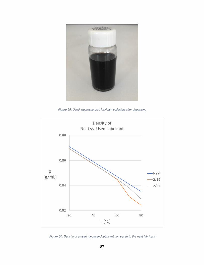
87

Figure 59: Used, depressurized lubricant collected after degassing

Figure 60: Density of a used, degassed lubricant compared to the neat lubricant

88

The density of the degassed lubricant was measured with an Anton-Paar SVM 3000

Viscometer-Densitometer with an uncertainty of 0.00005 g/cm³ for density measurements. This

was done at temperatures from 20-80°C (68-176°F) with the results shown in Figure 60.

Looking at Figure 60 in detail, one notes that the used lubricant had a density that was slightly

lower than the neat lubricant up to a temperature of 60°C. At temperatures above 60°C, the

density began to diverge from the linearity seen at lower temperatures. Upon inspection, it was

noted that bubbles were forming in the densitometer at temperatures above 60°C indicating that

there was some gas still dissolved in the lubricant even after the degassing process. This

indicates that this method for determining solubility may not be ideal and the author points to the

use of viscosity mixing rules and the data from Seeton (2019) as a better source as described in

section 3.5 - Viscosity - Comparison with Previous Work. Following is a list of potential sources

of error in the current study and potential mitigation techniques for future studies.

1) Hydrocarbon gases are still entrained in the lubricant sample after pre-heating and

depressurization into an evacuated chamber. Future researchers should identify better

separation techniques than those listed here.

2) The sampling process allowed partial flashing of the samples allowing some dissolved

gas to come out of solution. This could be mitigated by using a sampling cylinder with

back-pressure regulation capabilities.

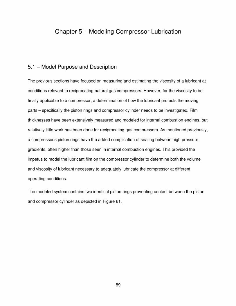
89

Chapter 5 – Modeling Compressor Lubrication

5.1 – Model Purpose and Description

The previous sections have focused on measuring and estimating the viscosity of a lubricant at

conditions relevant to reciprocating natural gas compressors. However, for the viscosity to be

finally applicable to a compressor, a determination of how the lubricant protects the moving

parts – specifically the piston rings and compressor cylinder needs to be investigated. Film

thicknesses have been extensively measured and modeled for internal combustion engines, but

relatively little work has been done for reciprocating gas compressors. As mentioned previously,

a compressor’s piston rings have the added complication of sealing between high pressure

gradients, often higher than those seen in internal combustion engines. This provided the

impetus to model the lubricant film on the compressor cylinder to determine both the volume

and viscosity of lubricant necessary to adequately lubricate the compressor at different

operating conditions.

The modeled system contains two identical piston rings preventing contact between the piston

and compressor cylinder as depicted in Figure 61.

90

Figure 61: Diagram of the compressor piston-cylinder system modeled. Note: components in diagram are not to scale

The two piston rings create three volumes where gas is trapped. Volumes 1 and 3 cycle

between just below the suction pressure and just above the discharge pressure while volume 2

cycles between two intermediate pressures. The data for the model was extracted from Hanlon

(2001) and is shown in Figure 62 with the horizontal, black lines representing the discharge

pressure (upper line) and suction (lower line) pressure.

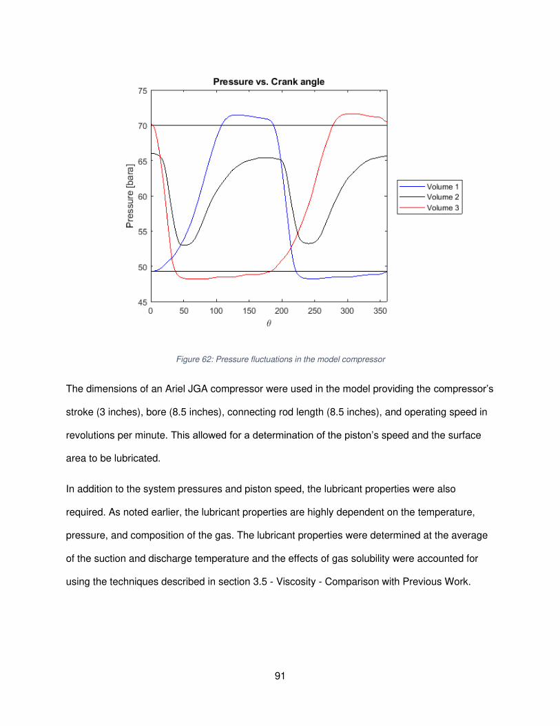
91

Figure 62: Pressure fluctuations in the model compressor

The dimensions of an Ariel JGA compressor were used in the model providing the compressor’s

stroke (3 inches), bore (8.5 inches), connecting rod length (8.5 inches), and operating speed in

revolutions per minute. This allowed for a determination of the piston’s speed and the surface

area to be lubricated.

In addition to the system pressures and piston speed, the lubricant properties were also

required. As noted earlier, the lubricant properties are highly dependent on the temperature,

pressure, and composition of the gas. The lubricant properties were determined at the average

of the suction and discharge temperature and the effects of gas solubility were accounted for

using the techniques described in section 3.5 - Viscosity - Comparison with Previous Work.

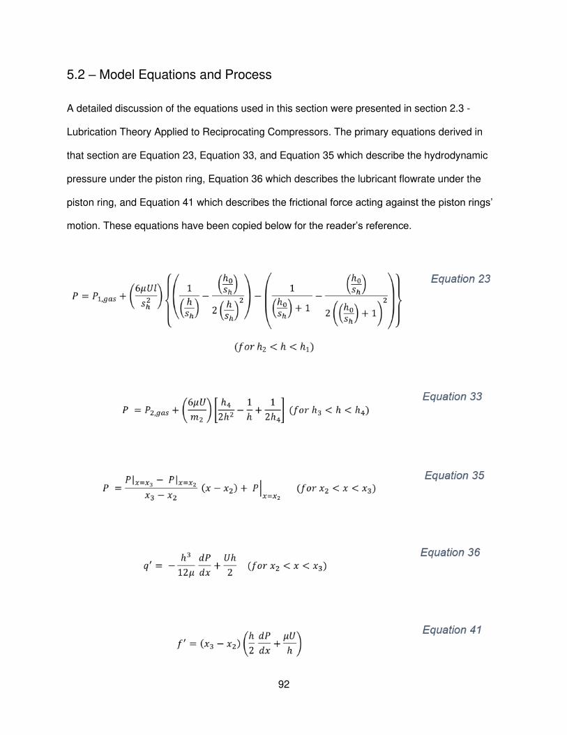
92

5.2 – Model Equations and Process

A detailed discussion of the equations used in this section were presented in section 2.3 -

Lubrication Theory Applied to Reciprocating Compressors. The primary equations derived in

that section are Equation 23, Equation 33, and Equation 35 which describe the hydrodynamic

pressure under the piston ring, Equation 36 which describes the lubricant flowrate under the

piston ring, and Equation 41 which describes the frictional force acting against the piston rings’

motion. These equations have been copied below for the reader’s reference.

93

The equations all depend on a set of variables which define the inputs to the model, and we

group these by where the variables come from physically:

1. Piston ring geometry: The variables 𝑙, 𝑠ℎ ,𝑚2, 𝑥2, and 𝑥3 all depend on the geometry of

the piston ring as described in detail in section 2.3 - Lubrication Theory Applied to

Reciprocating Compressors.

2. Compressor size and speed: The variable 𝑈 represents the speed of the piston ring

which will vary throughout the compressor’s stroke reaching up to 5.9 m/s (1167

feet/min) in some compressors. This variable depends on many compressor specifics

requiring new variables including: the length of the compressor’s stroke (𝑆), the length of

the compressor’s connecting rod (𝐿), and the speed of the compressor’s crankshaft (𝑟𝑝𝑚). Integral engine-compressors run as slow as 200 rpm (Sloan, 2018) while newer

compressors can operate at speeds up to 1800 rpm. In addition to this, the compressor’s

bore (𝐵) will aid in determining the volume of lubricant flowing under the piston ring as

well as the friction force acting on the piston ring.

3. Compressor application: The variables 𝑃1,𝑔𝑎𝑠 and 𝑃2,𝑔𝑎𝑠 depend on the suction and

discharge pressure of the specific compressor application and the fluctuation between

these pressures during the compression or suction stroke. In addition to this, the

compressor’s operating temperature (𝑇) is assumed to be the average of the suction

and discharge gas temperatures and the gas composition (𝜒𝑖) will impact the lubricant’s

viscosity.

4. Lubricant properties: The variable 𝜇 represents the lubricant’s viscosity which will

depend on the compressor’s operating temperature, gas pressure, and gas composition

as described in detail in previous sections.

A flow chart of how the input variables are used is presented in Figure 63.

94

Figure 63: Flow chart describing model inputs usage

The careful reader will note that we still have not addressed one variable: the lubricant film

thickness. This is represented by the variable ℎ and is by far the most important variable as

every equation depends on it. This variable cannot be solved for analytically as it must be found

by equilibrating the hydrodynamic force under the piston ring with the force on top of the piston

ring as shown in Figure 64. The solution procedure to calculate the film thickness is shown in

Figure 65.

95

Figure 64: Forces acting on the compressor piston ring

Figure 65: Film thickness iterative solution procedure

96

Once the film thickness has been determined, it can be used with the compressor bore and

Equation 36 and Equation 41 to determine the flowrate under the piston ring and the friction

force as shown in Figure 66.

Figure 66: Procedure to calculate the lubricant flow rate and friction force

As noted in Figure 66, this procedure is done for each Crank-Angle-Degree (CAD) in the

compressor’s stroke allowing for a determination of the film thickness, lubricant flow rate, and

friction force along the entire stroke. The friction force is easily converted to a power loss by

multiplying the friction force by the piston’s instantaneous speed.

5.3 – Results of Modeling work

The model contains many variables to account for different compressor sizes and operating

conditions. However, the interest of this section was to determine the effects of just two

variables: the lubricant viscosity and the amount of lubricant on the cylinder wall. Thus, it was

necessary to hold all other variable constant and a system was modeled with a suction pressure

of 49.3 bara (700 psig), a discharge pressure of 70 bara (1000 psig), a mean temperature of

100°C (212°F) with the compressor dimensions mentioned previously operating at 1000 rpm.

The viscosity of the lubricant and the volume of lubricant were then varied independently to

determine how those two factors impacted the compressor’s lubrication.

97

5.3.1 – Lubricant Viscosity

As discussed in section 2.3 - Lubrication Theory Applied to Reciprocating Compressors,

increasing the lubricant’s viscosity increases the separation gap or lubricant film thickness

between the moving parts. In relation to reciprocating compressors, the purpose of this film is to

prevent asperity contact between the piston ring and the compressor cylinder wall. It is common

to assume that a lubricant film that is three times thicker than the average roughness of the

moving parts will provide proper, hydrodynamic lubrication. A contact familiar with the machining

process at Ariel Inc. (C. Lingel, personal communication, 2020) indicated that the compressor

cylinder bore has an average roughness of 0.813 microns (32 microinches). This implies that a

lubricating film thickness of at least 2.44 microns (96 microinches) is required to properly

prevent contact between the compressor cylinder wall and piston rings.

To investigate how a lubricant’s viscosity affects the film thickness, lubricant flow rate, and

power loss, the viscosity was varied across a range of values. For the reader’s reference, liquid

water at 100°C has a viscosity around 0.3 cP. Additionally, the data from Seeton (2019)

measured the viscosity of Mobil Pegasus 805 Ultra to be 7.65 cP when diluted with pure

methane at 70 bara (1000 psig) and 100°C (212°F) while PROGILINE® LPG-WS-150 from

Shrieve Chemical had a viscosity of 20.86 cP at the same conditions. Viscosity values of 0.3,

7.65, and 20.86 cP were chosen to show the effects of the lubricant’s viscosity with results

shown in Figure 67, Figure 68, and Figure 69.

98

Figure 67: Film thicknesses for varying viscosities

Figure 67 shows the expected trend: increasing the lubricant viscosity increases the lubricant

film thickness. Looking at Figure 67 in detail shows that every lubricant produces a film

thickness that is too small to prevent asperity contact for at least part of a cycle. However,

comparing the amount of the cycle that the piston spends properly lubricated shows the

importance of using a lubricant with the proper viscosity as shown in Table 10.

Table 10: Amount of cycle that is properly lubricated vs. the lubricant's viscosity

Viscosity [cP] Reference Fluid % of Stroke with Adequate Lubrication

0.3 Water 1.1%

7.65 Pegasus 805 Diluted Methane 40.2%

20.86 PROGILINE® LPG WS-150 Diluted Methane 77.6%

0

5

10

15

20

25

30

0 90 180 270 360

Film Thickness

[µm]

CAD

Film Thickness vs. CAD

Water

Pegasus 805 Ultra

Progiline WS-150

Asperity Contact

99

Table 10 shows that selecting a lubricant with a higher viscosity protects the piston rings and

compressor cylinder over a larger fraction of the piston’s motion. Additionally, Hanlon (2001)

claimed that “when lubricating oil reaches the viscosity equivalent to water, the oil film no longer

supports dynamic loads resulting in rapid failure” and this is indeed validated by the results

shown in Table 10. Going off viscosity alone indicates that a lubricant with a higher viscosity

should be selected for every application. However, increasing the viscosity also increases the

volume of lubricant flowing under the piston ring and the frictional power losses in the

compressor – both of which may be undesirable.

Figure 68: Lubricant flowrates for varying lubricant viscosities

-0.003

-0.002

-0.001

0

0.001

0.002

0.003

0.004

0.005

0 90 180 270 360

Flowrate

[mL/CAD]

CAD

Flowrate vs. CAD

Water

Pegasus 805 Ultra

Progiline WS-150

100

Figure 69: Frictional power loss for varying lubricant viscosities

Figure 68 and Figure 69 also show the expected trends: increasing the lubricant viscosity

increases the volume of lubricant flowing under the piston ring, and the frictional power loss.

Although these increases may seem detrimental at first, they must be kept in comparison to the

benefit provided as shown in Table 10. Thus, Table 11 and Table 12 are presented for

comparison.

Table 11: Increase in total volume of lubricant required to lubricate one cycle vs. the lubricant's viscosity

Viscosity [cP] Reference Fluid Total Lubricant Volume per cycle [mL]

0.3 Water 0.03

7.65 Pegasus 805 Diluted Methane 0.13

20.86 PROGILINE® LPG WS-150 Diluted Methane 0.21

0

100

200

300

400

500

600

700

0 90 180 270 360

Frictional

Power Loss

[W]

CAD

Power Loss vs. CAD

Water

Pegasus 805 Ultra

Progiline WS-150

101

Table 12: Increase in average power loss during one cycle vs. the lubricant's viscosity

Viscosity [cP] Reference Fluid Mean Power Loss [W]

0.3 Water 30

7.65 Pegasus 805 Diluted Methane 153

20.86 PROGILINE® LPG WS-150 Diluted Methane 253

For a simple comparison, Table 10 shows that increasing the lubricant viscosity from 7.65 to

20.86 cP nearly doubles the amount of the cycle that is properly lubricated (93% increase).

Table 11 and Table 12 show that this same increase in viscosity does not approach the same

increase in the volume of lubricant flowing under the piston ring (a 62% increase) or the average

power loss over the cycle (a 65% increase). To put the power losses into perspective, the JGA

compressor that was modeled is rated at 140 horsepower per throw (Ariel Corporation). The

mean power losses shown in Table 12 equate to 0.04, 0.21, and 0.34 horsepower for water,

Mobil Pegasus 805 Ultra, and PROGILINE® LPG WS-150 respectively. Thus, increasing the

lubricant’s viscosity (including dilution effects) is an effective method for preventing wear to the

moving parts with minimal side effects. However, this section has only considered situations

where there is an adequate amount of lubricant on the compressor cylinder to fully flood the

inlet of the compressor piston ring – what happens if not enough lubricant is supplied to the

cylinder or the lubricant is washed from the cylinder wall before it is used?

5.3.2 – Lubricant Volume

The previous section only considered the case when the piston ring is “fully flooded” which

implies that there is a sufficient volume of lubricant ahead of the piston ring to fully fill the cavity

under the leading edge of the piston ring. This is in contrast to a “starved” condition where there

102

is an insufficient volume of lubricant ahead of the piston ring such that the leading edge of the

piston ring is not entirely filled with lubricant. The two conditions are depicted in Figure 70.

Figure 70: Comparison of fully flooded (left) and starved (right) lubrication conditions

Whether or not the gap on the leading edge is fully filled with lubricant makes a large difference

on the hydrodynamic pressure built up under the piston ring which impacts the separation gap

between the moving parts. Varying the lubricant starvation allows for a better comparison

between dissimilar lubricants. Figure 68 showed that a larger volume of lubricant could flow

under the piston ring for a lubricant with a higher viscosity which implies that more lubricant is

required for a fully flooded condition. Increasing the starvation for the lubricant with the higher

viscosity allows for a comparison of how the compressor is lubricated with the same volume of

lubricant as shown in Figure 71.

103

Figure 71: Effect of lubricant starvation. Compressor lubrication using the same volume of lubricant.

Figure 71 shows that using a lubricant with a higher viscosity provides protection from asperity

contact over a larger portion of the stroke as compared to a lower viscosity lubricant (58%

above the asperity contact line as compared to 45%). This implies that the higher viscosity

lubricant is used more efficiently on a volumetric basis. Moving on from this comparison, it is

also possible to increase the starvation of the higher viscosity lubricant such that the lubricants

both protect the compressor over the same percentage of the stroke as shown in Figure 72.

0

4

8

12

16

20

0 45 90 135 180

Film Thickness

[µm]

CAD

Effects of Starvation

Flooded - Pegasus 805 Ultra

Starved - Progiline WS-150

Asperity Contact

104

Figure 72: Effect of lubricant starvation. Providing similar compressor protection with a lower volume of lubricant.

Calculating the total volume of the lubricant used in the two cases shown in Figure 72 shows a

9% reduction in the volume of lubricant required by the higher viscosity lubricant. This shows

that selecting a lubricant with a higher viscosity makes it possible to reduce lubricant

consumption in a compressor while still providing the same protection to the compressor

cylinder and piston rings. Comparing the amount of the cycle that the piston is properly

lubricated provides a useful metric for comparing different operating conditions. Varying the

percent of the inlet gap that is fully flooded for the two lubricants produces Figure 73.

0

4

8

12

16

20

0 45 90 135 180

Film Thickness

[µm]

CAD

Reduced Lubricant Consumption

Flooded - Pegasus 805 Ultra

Starved - Progiline WS-150

Asperity Contact

105

Figure 73: Percent of cycle adequately lubricated depending on starvation condition

Figure 71, Figure 72, and Figure 73 all demonstrate that choosing a lubricant with a higher

viscosity is important to providing proper lubrication over a larger portion of the piston’s motion

but an insufficient amount any lubricant will reduce the time the piston is adequately lubricated.

This makes it apparent that the amount of lubricant on the cylinder wall can be just as important

as the viscosity of the lubricant. This work has focused on the viscosity of the lubricant and its

impact on proper compressor lubrication, but how can an operator be sure that there is a

sufficient amount of lubricant on the cylinder wall? Part of the answer is that the operator must

be sure that the lube rate is high enough to supply lubricant to the compressor cylinder.

However, this only captures half of the answer as the operator needs to balance this lube rate

with the rate at which the lubricant is removed from the cylinder. Simple calculations show that

for the modeled lubricants, the lubricant on the cylinder wall is not removed on every stroke as

that would imply 373-607 liters (99-160 gallons) of lubricant would be consumed each day. The

rate at which the lubricant is removed from the cylinder wall will depend on how the gas stream

washes the lubricant from the cylinder wall in addition to the fluid dynamics of how the lubricant

flows down to the compressor valves. Experimental work investigating how liquid heptane

0%

20%

40%

60%

80%

100%

0% 20% 40% 60% 80% 100%

% of Stroke

Adequately

Lubricated

% Fully Flooded

% of Stroke Adequately Lubricated vs.

% of Fully Flooded Condition

Progiline WS-150

Pegasus 805 Ultra

106

washes a lubricant from the cylinder wall was presented by Matthews (1987) but the literature is

rather scarce about addressing how a gas stream can wash away a lubricant with little more

than mentions of this idea existing in the literature (Vanderkelen, King, & Batch, 1974).

Experimental or modeling studies investigating how lubricant flows down the compressor

cylinder and how different gas streams may wash a lubricant from the cylinder wall should be

investigated in greater detail to provide a better understanding of proper lubrication rates.

107

Chapter 6 – Suggestions for Lubricants and Lubrication Rates for

Reciprocating Compressors

Following is a summary of the results presented in this thesis, how the results of the current

study relate to the current methods used in the natural gas compression industry, and ideas for

future areas of study.

6.1 – Compressor Lubricant Viscosity – Comparisons and Suggestions

The viscosity of a lubricant is one of the most important properties when selecting a lubricant for

a reciprocating compressor. However, high pressure gases can dilute lubricants, reducing their

viscosity. This thesis has presented and validated methods to calculate the viscosity of a

lubricant diluted with a natural gas mixture combining the work of Seeton (2009), (2019) with an

ideal mixing assumption as presented in section Chapter 3 – Lubricant Absorption of Natural

Gas – Results from the Laboratory. Seeton (2019) details accurate measurements for Mobil

DTE Extra Heavy, Mobil Pegasus 805 Ultra, and PROGILINE® LPG-WS-150 from Shrieve

Chemical. Mixture viscosities have been validated in this work for Mobil Pegasus 805 Ultra, but

the author suggests that this method should apply for other two lubricants as well. Extrapolation

of this data from Seeton (2019) to other lubricants should be investigated in more detail

acknowledging that the Mobil products are mineral oils (MOs) and the Shrieve product is a

polyalkylene glycol (PAG).

In addition to calculating the viscosity of a lubricant diluted with natural gas, this work also

presented a model capable of calculating the lubricant film thickness in a reciprocating

compressor in Chapter 5 – Modeling Compressor Lubrication. This model takes into

consideration the size and operating conditions of the compressor in addition to the properties

108

of the lubricant including the dilution effect. This method allows an operator to calculate the

minimum viscosity required for their compressor to ensure that asperity contact is not a common

occurrence for their specific operating conditions.

A review of current knowledge of this topic is presented in section 2.1. This work compares well

with current industry experience in the following ways:

• Hanlon (2001) notes that “when lubricating oil reaches the viscosity equivalent to water,

the oil film no longer supports dynamic loads resulting in rapid failure” and this is indeed

validated by the results shown in Table 10.

• Ariel Corporation and Dresser-Rand (A Siemens Business) both present methods to

select a lubricant based on the operating conditions. Ariel uses the gas composition and

pressure as shown in (Table 4) and Dresser-Rand uses the discharge pressure,

temperature, and the potential to find liquids in the gas (Table 5). Liquids in the gas

refers to the phenomenon of washing and is not considered in this work. However, the

rest of these factors are all accounted for in the methods described in Chapter 3 –

Lubricant Absorption of Natural Gas – Results from the Laboratory.

• Ariel Corporation, Dresser-Rand (A Siemens Business), and Sloan (2018) all indicate

that the Cigarette Paper Test provides a method to determine proper lubricant rates but

not proper lubricant viscosity which is easily validated with the methods discussed here

in combination with the work of Seeton (2019).

In making suggestions for lubricant viscosity requirements for reciprocating compressor, the

author focuses on the results of Chapter 5 – Modeling Compressor Lubrication. This section

shows that increasing the lubricant viscosity substantially increases the lubricant film thickness

providing protection for the compressor components over a larger portion of the piston’s motion.

The average power loss and total lubricant volume required for adequate lubrication do not

increase linearly with the increase in compressor protection. Rather, the average power loss

109

and total lubricant volume increase less rapidly than the increase in compressor protection

implying that a lubricant with a higher viscosity should always be selected when possible with

the caveat that there are diminishing returns on protection as the viscosity increases.

6.2 – Compressor Lubrication Rates – Comparisons and Suggestions

In addition to selecting the correct lubricant viscosity, adding an adequate amount of lubricant to

the compressor is necessary. The use of too little lubricant can have the same results as using

a lubricant with a low viscosity – increased wear and reduced component lifetime. Again, current

knowledge of this topic is presented in section 2.1. This work compares well with current

industry experience in the following ways:

• Hanlon (2001) presents a figure (Figure 74) on how the lifetime of piston rings and

packings depend on an unscaled lube rate. Though not an exact comparison, this trend

corresponds very well with Figure 75 which correlates the amount of the piston’s stroke

that is properly lubricated versus the how close the piston ring is to obtaining a fully

flooded inlet condition.

Figure 74: A comparison of packing and piston ring lifetime versus lube rate from (Hanlon, 2001), copy of Figure 10

110

Figure 75: Percent of cycle adequately lubricated depending on starvation condition, copy of Figure 73

• Hanlon (2001), Ariel Corporation, Dresser-Rand (A Siemens Business), and Sloan

(2018) all account for the surface area that requires lubrication. Ariel Corporation does

make not explicit mention of the compressor’s operating speed and focuses only on the

compressor’s bore size. Hanlon, Dresser-Rand, and Sloan all account for the

compressor’s bore size and operating speed. All four sources indicate that increasing

the bore size increases the required lubrication rate. Hanlon, Dresser-Rand, and Sloan

indicate that increasing the compressor’s speed also increases the required lubrication

rate. The model presented in this thesis agrees qualitatively with both results. This is

demonstrated by the appearance of the bore size in the equations. The equations also

show that the compressor’s speed increases the lubricant film thickness which requires

more lubricant to fully flood the piston ring inlet at higher operating speeds.

• Quantitative correlations were made in Chapter 5 – Modeling Compressor Lubrication for

suggesting lubrication rates. However, a simple calculation was presented for the

volume of lubricant required for every cycle and how much lubricant would be required

0%

20%

40%

60%

80%

100%

0% 20% 40% 60% 80% 100%

% of Stroke

Adequately

Lubricated

% Fully Flooded

% of Stroke Adequately Lubricated vs.

% of Fully Flooded Condition

Progiline WS-150

Pegasus 805 Ultra

111

per day if this volume of lubricant was removed on every stroke. This gave an upper

bound for the maximum amount of lubricant a compressor could need in a day and was

high above the lubrication rates presented by Hanlon, Ariel Corporation, Dresser-Rand,

and Sloan.

6.3 – Suggestions for Future Work

This thesis focused on measuring and calculating the viscosities of lubricants diluted with

natural gas at pressures and temperatures seen in operating compressors and how the

viscosity impacted the lubricant film thickness and protection of the compressor’s piston rings

and cylinder wall. The topic of lubrication rates was not investigated to the same depth and the

author would like to suggest areas for future that could have the most impact for correlating

lubrication rates to operating conditions.

6.3.1 – Lubricant Foaming and Atomization into Gas Stream

The required lube rate in the compressor cylinder should roughly, if not exactly, equal the rate at

which lubricant is removed from the compressor cylinder. The rate at which a gas stream

removes a lubricant from the cylinder wall has not, to the best of this author’s knowledge, been

investigated in detail. It is suspected that the rate at which a lubricant is removed from the

cylinder wall will depend on the lubricant’s viscosity and surface tension in addition to the gas

solubility in the lubricant. Lubricants may foam when the pressure in the cylinder is reduced

presenting the opportunity for the lubricant to be atomized into the gas stream. These properties

will all depend on the specific lubricant and gas composition under consideration in addition to

the pressure and temperature at which these analyses are conducted. Experimental or

modeling studies investigating how gas-lubricant mixtures behave when depressurized under

different conditions may provide a better understanding of proper lubrication rates.

112

6.3.2 – Lubricant Washing with Liquid in Gas Stream

Experimental work investigating how liquid heptane washes a lubricant from the cylinder wall

was presented by Matthews (1987) but these tests were conducted at room temperature and

pressure. The literature is rather scarce about addressing how a gas stream can wash away a

lubricant. A variety of gas compositions and lubricants should be investigated to see the effects

of washing a MO or PAG lubricant with a natural gas saturated with water, carbon dioxide, or

heavy hydrocarbons. Experimental or modeling studies should investigate how liquids in the gas

stream can wash lubricant off the cylinder wall at temperatures and pressures relevant to

operating compressors to provide a better understanding of proper lubrication rates.

6.3.3 – Modeling Lubricant Fluid Dynamics

Although the Reynold’s equation is presented as the governing equation for the modeling work

in this thesis, it is noted that the effects of gravity will be important for long-term lubricant flow

rates. Compressor discharge valves lie on the lower half of the cylinder and thus the lubricant

will move towards these valves over time. Modeling or experimental work investigating how the

lubricant’s viscosity impacts the rate at which the lubricant travels down the compressor cylinder

could provide valuable insight for selecting proper lubrication rates.

113

Bibliography

Ariel Corporation. (2020, December). JGU-JGZ Manual - Section 3 - Maintenance. Retrieved

from Ariel Corporation: https://www.arielcorp.com/Support/Manuals/JGU-JGZ/Section-3/

Ariel Corporation. (n.d.). ARIEL NATURAL GAS COMPRESSORS. Retrieved 2019, from Ariel

Corporation: https://www.arielcorp.com/compressors/compressor-landing-page.html

Ariel Corporation. (n.d.). DOWNSTREAM & REFINERY. Retrieved from Ariel Corporation:

https://www.arielcorp.com/compressors/compressor-applications/downstream-and-

refinery.html

Ariel Corporation. (n.d.). The Ariel JG/JGA. Retrieved 2021, from Ariel Corporation:

https://www.arielcorp.com/compressors/compressor-landing-page/jg-jga.html

ASTM International. (2016). D2270-10(2016) Standard Practice for Calculating Viscosity Index

from Kinematic Viscosity at 40 °C and 100 °C. Retrieved from

https://compass.astm.org/EDIT/html_annot.cgi?D2270+10(2016)

ASTM International. (2016). D7152-11(2016)e1 - Standard Practice for Calculating Viscosity of

a Blend of Petroleum Products. doi:doi: https://doi.org/10.1520/D7152-11R16E01

ASTM International. (2020). D2779-92(2020) Standard Test Method for Estimation of Solubility

of Gases in Petroleum Liquids. Retrieved from Retrieved from

https://doi.org/10.1520/D2779-92R20

ASTM International. (2020). D341 - 20e1 - Standard Practice for Viscosity-Temperature

Equations and Charts for Liquid Petroleum or Hydrocarbon Products.

doi:https://doi.org/10.1520/D0341-20E01

ASTM International. (2020). D3827 - 92(2020) Standard Test Method for Estimation of Solubility

of Gases in Petroleum and Other Organic Liquids. Retrieved from

https://compass.astm.org/EDIT/html_annot.cgi?D3827+92(2020)

Barus, C. (1893). Isothermals, isopiestics and isometrics relative to viscosity. American Journal

of Science, 45, 87-96. Retrieved from

https://search.proquest.com/openview/e14e9b6e42a1eb160fdf32c89ffd3280/1/advanced

114

Battino, R. (1984). THE OSTWALD COEFFICIENT OF GAS SOLUBILITY. Fluid Phase

Equilibria, 231-240. Retrieved from

https://www.sciencedirect.com/science/article/pii/0378381284870090?via%3Dihub

Battino, R., & Clever, H. L. (1966). The Solubility of Gases in Liquids. Chemical Reviews, 395-

463. Retrieved from https://pubs.acs.org/doi/10.1021/cr60242a003

Berthezene, N., Hemptinne, J. d., Audibert, A., & Argillier, J. F. (1999). Methane solubility in

synthetic oil-based drilling muds. Journal of Petroleum Science and Engineering, 71-81.

Retrieved from https://www.sciencedirect.com/science/article/pii/S092041059900008X

Brun, K. (2018, October). The US Natural Gas Compression Infrastructure: Opportunities for

Efficiency Improvements. Retrieved from netl.doe.gov:

https://netl.doe.gov/sites/default/files/netl-file/Brun.pdf

Burckhardt Compression. (2021). COMPRESSOR COMPONENTS. Retrieved February 11,

2021, from Burckhardt Compression:

https://www.burckhardtcompression.com/media/downloads/compressor-components/

Cambridge Viscosity. (2012). In-Line Explosion Proof Sensors - Viscosity Sensors.

Czubinski, F. F., Sanchez, C. J., Silva, A. K., Neto, M. A., & Barbosa, Jr., J. R. (2020). Phase

equilibrium and liquid viscosity data for R-290/POE ISO 22 mixtures between 283 and

353 K. International Journal of Refrigeration, 114, 79-87.

doi:https://doi.org/10.1016/j.ijrefrig.2020.02.029.

Dresser-Rand (A Siemens Business). (2015). Packager Guidelines, Index. Retrieved February

2, 2021, from https://assets.new.siemens.com/siemens/assets/api/uuid:ac0df0e9-308b-

478f-8c12-35a36a3526c4/complete-packager-guidelines.pdf

Enbridge Gas Inc. (2021). Chemical Composition of Natural Gas. Retrieved from

UnionGas/Enbridge: https://www.uniongas.com/about-us/about-natural-gas/chemical-

composition-of-natural-gas

Eser, S. (n.d.). Natural Gas Composition and Specifications. Retrieved February 9, 2021, from

PennState - FSC 432 - Petroleum Processing: https://www.e-

education.psu.edu/fsc432/content/natural-gas-composition-and-specifications

115

Fatjo, G. G.-A., Smith, E. H., & Sherrington, I. (2018). Piston-ring film thickness: Theory and

experiment compared. Journal of Engineering Tribology, 232(5), 550–567. Retrieved

from https://journals.sagepub.com/doi/full/10.1177/1350650117722257

Feng, J., Fu, J., Chen, P., Du, Z., & Qin, L. (2016). Experimental study and molecular simulation

of gas dissolution and diffusion behavior in drilling fluid. Journal of Natural Gas Science

and Engineering, 424-433. Retrieved from

https://www.sciencedirect.com/science/article/pii/S1875510016307983

Frolich, K., Tauch, E. J., Hogan, J. J., & Peer, A. A. (1931). Solubilities of Gases in Liquids at

High Pressure. INDUSTRIAL AND ENGINEERING CHEMISTRY, 23(5), 548-550.

Retrieved from https://pubs.acs.org/doi/pdf/10.1021/ie50257a019

G.E. Totten, G. T., & R. J. Bishop, D. C. (2002, September). Natural Gas Compressor

Maintenance and Lubricant Requirements. Retrieved from Machinery Lubrication:

https://www.machinerylubrication.com/Read/393/natural-gas-compressors-maintenance

Hamrock, B. J., Schmid, S. R., & Jacobson, B. O. (2004). Fundamentals of Fluid Film

Lubrication (Second ed.). USA: Marcei Dekker, Inc. doi:ISBN: 0-8247-5371-2

Hanlon, P. C. (Ed.). (2001). Compressor Handbook. McGraw-Hill Companies, Inc.

Hill, E. S. (1934). The Rate of Solution of Methane and Propane in Hydrocarbon Oils. Doctoral

Thesis. Retrieved from https://thesis.library.caltech.edu/10728/1/Hill_WC_1934.pdf

Hosgormez, H., Etiope, G., & Yalcin, M. N. (2008). New evidence for a mixed inorganic and

organic origin of the Olympic Chimaera fire (Turkey): a large onshore seepage of

abiogenic gas. Geofluids, 8(4), 263-273. doi:https://doi.org/10.1111/j.1468-

8123.2008.00226.x

Kruse, H. (1974). Calculation of the Hydrodynamic Lubrication of Piston and Piston Rings in

Refrigeration Compressors. International Compressor Engineering Conference. Paper

101. Retrieved from https://docs.lib.purdue.edu/icec/101

Lacey, W. N., Sage, B. H., & Kircher, Jr., C. E. (1934). Phase Equilibria in Hydrocarbon

Systems III. Solubility of a Dry Natural Gas in Crude Oil. INDUSTRIAL AND

ENGINEERING CHEMISTRY, 26(6), 652-654. Retrieved from

https://pubs.acs.org/doi/pdf/10.1021/ie50294a014

116

Markham, A. E., & Kobe, K. A. (1941). THE SOLUBILITY OF GASES IN LIQUIDS. Chemical

Reviews, 519-588. Retrieved from https://doi.org/10.1021/cr60091a003

Matthews, P. (1987). Lu b ricat i on of Rec i p roc at i ng Compressors. Chester,England: Shell

Research Ltd,Thornton Research Centre. Retrieved from

https://onlinelibrary.wiley.com/doi/abs/10.1002/jsl.3000050404

Merriam-Webster. (n.d.). Viscosity. Retrieved 02 08, 2021, from https://www.merriam-

webster.com/dictionary/viscosity

Mokhatab, S., Poe, W. A., & Mak, J. Y. (2015). Chapter 3 - Basic Concepts of Natural Gas

Processing. In Handbook of Natural Gas Transmission and Processing (Third Edition)

(Third ed., pp. 123-135). Gulf Professional Publishing. doi:https://doi.org/10.1016/B978-

0-12-801499-8.00003-1

National Geographic. (2001, August 14). Delphic Oracle's Lips May Have Been Loosened by

Gas Vapors. Retrieved from National Geographic/Science:

https://www.nationalgeographic.com/science/2001/08/greece-delphi-oracle-gas-vapors-

science/

Neto, M. A., & Barbosa, Jr., J. R. (2008, January). Solubility, density and viscosity of a mixture

of R-600a and polyol ester oil. International Journal of Refrigeration, 31(1), 34-44.

Retrieved from https://www.sciencedirect.com/science/article/pii/S0140700707001624

O'bryan, P. L. (1988, May). Well Control Problems Associated With Gas Solubility in Oil-Based

Drilling Fluids. Retrieved from

https://digitalcommons.lsu.edu/cgi/viewcontent.cgi?referer=https://scholar.google.com/&

httpsredir=1&article=5523&context=gradschool_disstheses

Overgaard, H. T. (2018, September). Lubricant Transport across Piston Rings in Large Two-

Stroke Diesel Engines - Theory and Experiments. PhD Thesis.

Ribeiro, P. R., Pessôa-Filho, P. A., Lomba, R. F., & J.Bonet, E. (2006). Measurement and

modeling of methane dissolution in synthetic liquids applied to drilling fluid formulation

for deep and ultradeep water wells. Journal of Petroleum Science and Engineering,

51(1-2), 37-44. Retrieved from


117

Sage, B. H., Davies, J. A., Sherborne, J. E., & Lacey, W. N. (1936). Phase Equilibria XVII.

Ethane-Crystal Oil System. INDUSTRIAL AND ENGINEERING CHEMISTRY, 28(11), -

1333. Retrieved from https://pubs.acs.org/doi/pdf/10.1021/ie50323a023

Sage, B. H., Lacey, W. N., & Schaafsma, J. G. (1934). Phase Equilibria in Hydrocarbon

Systems IV. Solubility of Propane in Two Different Oils. INDUSTRIAL AND

ENGINEERING CHEMISTRY, 26(8), 874-877. Retrieved from

https://pubs.acs.org/doi/pdf/10.1021/ie50296a016

Schlumberger. (2021). wet gas. Retrieved from Explore the new Oilfield Glossary:

https://www.glossary.oilfield.slb.com/en/terms/w/wet_gas

Scott, R. (2003, November). Reciprocating Natural Gas Compressors. Retrieved from

Machinery Lubrication: https://www.machinerylubrication.com/Read/552/reciprocating-

natural-gas-compressors

Seeton, C. J. (2009). CO2-LUBRICANT TWO-PHASE FLOW PATTERNS IN SMALL

HORIZONTAL WETTED WALL CHANNELS; THE EFFECTS OF

REFRIGERANT/LUBRICANT THERMOPHYSICAL PROPERTIES. DISSERTATION.

Retrieved from https://www.ideals.illinois.edu/handle/2142/83940

Seeton, C. J. (2019). Lubricants for Industrial Natural Gas Compression – Oilfield, Pipeline, and

Separation Facilities. Gas Machinery Conference.

Siemens. (2014, September 22). Siemens announces agreement to acquire Dresser-Rand.

Munich, Germany. Retrieved from

https://press.siemens.com/global/en/pressrelease/siemens-announces-agreement-

acquire-dresser-rand

Sloan, C. J. (2018). Innovations in Compressor Cylinder and Rod Packing Lubrication:

Approaches and Results. Gas Machinery Conference.

Spauschus, H. O., & Henderson, D. R. (1990). New Methods of Determining Viscosity and

Pressure of Refrigerant/Lubricant. International Refrigeration and Air Conditioning

Conference. Paper 99. Retrieved from http://docs.lib.purdue.edu/iracc/99

Spauschus, H., Henderson, D., & Grasshoff, H. (1994). Lubricants for hydrocarbon refrigerants.

Proceedings of the IIF-IIR Conference, new applications of natural working fluids in

refrigeration and air conditioning, (p. 153). Hanover, Germany. doi:ISBN 2 903 633 68 1

118

Spectris, PLC. (2016). A Basic Introduction to Rheology. Retrieved 01 08, 2021, from

https://cdn.technologynetworks.com/TN/Resources/PDF/WP160620BasicIntroRheology.

pdf

Stewart, M. (2019). 9 - Reciprocating compressors. In Surface Production Operations Volume

IV - Pump and Compressor Systems: Mechanical Design and Specification (pp. 655-

778). doi:https://doi.org/10.1016/B978-0-12-809895-0.00009-0

Summers-Smith, D. (1967). SELECTION OF LUBRICANT VISCOSITY GRADE FOR

RECIPROCATING GAS COMPRESSORS. Proceedings of the Institution of Mechanical

Engineers, 182. Retrieved from

https://journals.sagepub.com/doi/pdf/10.1243/PIME_CONF_1967_182_401_02

Swearingen, J. S., & Redding, E. D. (1942). Viscosity Characteristics of Lubricating Oils

Saturated with Natural Gases at High Pressures. Industrial and Engineering Chemistry,

34(12), 1496-1498. Retrieved from https://pubs.acs.org/doi/pdf/10.1021/ie50396a017

Tanneberger, F., & Feldmann, J. (1983). Compression of Wet CO2 in Reciprocating

Compressors. SPE Annual Technical Conference and Exhibition.

doi:https://doi.org/10.2118/12207-MS

U.S. Energy Information Administration. (2008). About U.S. Natural Gas Pipelines -

Transporting Natural Gas . Retrieved from U.S. Energy Information Administration:

https://www.eia.gov/naturalgas/archive/analysis_publications/ngpipeline/index.html

U.S. Energy Information Administration. (2008). U.S. Natural Gas Pipeline Compressor Stations

Illustration, 2008. Retrieved from U.S. Energy Information Administration:

https://www.eia.gov/naturalgas/archive/analysis_publications/ngpipeline/compressorMap

.html

U.S. Energy Information Administration. (2009). U.S. Natural Gas Pipeline Network, 2009.

Retrieved from U.S. Energy Information Administration:

https://www.eia.gov/naturalgas/archive/analysis_publications/ngpipeline/ngpipelines_ma

p.html

U.S. Energy Information Administration. (2016, May 5). Hydraulically fractured wells provide

two-thirds of U.S. natural gas production. Retrieved from U.S. Energy Information

Administration: https://www.eia.gov/todayinenergy/detail.php?id=26112

119

U.S. Energy Information Administration. (2019, August 28). EIA updates its U.S. energy

consumption by source and sector chart. Retrieved from U.S. Energy Information

Administration:

https://www.eia.gov/todayinenergy/detail.php?id=41093#:~:text=In%202018%2C%20the

%20U.S.%20residential,%25)%20and%20electricity%20(50%25)

U.S. Energy Information Administration. (2021, January 29). NATURAL GAS - Natural Gas

Consumption by End Use. Retrieved from U.S. Energy Information Administration:

https://www.eia.gov/dnav/ng/ng_cons_sum_dcu_nus_a.htm

U.S. Energy Information Administration. (2021, January 2021). NATURAL GAS - U.S. Natural

Gas Gross Withdrawals. Retrieved from U.S. Energy Information Administration:

https://www.eia.gov/dnav/ng/hist/n9010us2A.htm

U.S. Energy Information Administration. (2021, January 15). Natural gas explained - Delivery

and storage of natural gas. Retrieved from U.S. Energy Information Administration:

https://www.eia.gov/energyexplained/natural-gas/delivery-and-storage.php

van Leeuwen, H. (2009). The determination of the pressure–viscosity coefficient of a lubricant

through an accurate film thickness formula and accurate film thickness measurements.

Journal of Engineering Tribology, 1143-1163.

doi:https://doi.org/10.1243/13506501JET504

Vanderkelen, J. B., King, F., & Batch, M. L. (1974). Compressor Lubrication. International

Compressor Engineering Conference, (p. Paper 104). Retrieved from

https://docs.lib.purdue.edu/cgi/viewcontent.cgi?article=1103&context=icec

Wang, X., Jia, X., & Wang, D. (2021). Experimental investigation on the solubility of R290 in two

mineral oils. International Journal of Refrigeration, 124, 13-19. Retrieved from


Wu, J., Chen, Z., Lin, J., & Li, J. (2018). Experimental analysis on R290 solubility and R290/oil

mixture viscosity in oil sump of the rotary compressor. International Journal of

Refrigeration, 94, 24-32. Retrieved from


Yance, Justin; Hagan, Joe; Ariel Corporation. (n.d.). Lube Reduction in Reciprocating

Compressors. Retrieved January 27, 2021, from Ariel Corporation:

120

http://ru.arielcorp.com/templates/SplitLayout.aspx?pageid=12884907236&rdr=true&Lang

Type=1049

Zhelezny, P. V., Zhelezny, V. P., Procenko, D. A., & Ancherbak, S. N. (2007). An experimental

investigation and modelling of the thermodynamic properties of isobutane–compressor

oil solutions: Some aspects of experimental methodology. International Journal of

Refrigeration, 30(3), 433-445. Retrieved from


THESIS RECIPROCATING COMPRESSOR LUBRICATION …

Documents

Transcript of THESIS RECIPROCATING COMPRESSOR LUBRICATION …