1

THERMOPHYSICS ’99

Meeting of the Thermophysical SocietyWorking Group of the Slovak Physical Society

Bratislava, October 22, 1999

Editor Libor Vozár

Constantine the Philosopher University in NitraFaculty of Natural Sciences

1999

2

© CPU Nitra, 1999

THERMOPHYSICS ‘99Proceedings of the Meeting of the Thermophysical Society - WorkingGroup of the Slovak Physical SocietyBratislava, October 22, 1999

Editor Libor Vozár

Issued by Constantine the Philosopher University in NitraFirst EditionReleased in 1999Printed by Car Print Nitra

Published with the support by the Slovak Science Grant Agency under the contract1/6115/99.

ISBN 80-8050-284-6

3

CONTENTS

PERFACE 5Ľudovít Kubičár

EFFECTIVE HEAT EQUATION IN PARTICULATE COMPOSITE 7Štefan Barta

MEASURING THE TEMPERATURE-DEPENDENT THERMALCONDUCTIVITY AND HEAT CAPACITY IN BUILDING MATERIALS 13Jozefa Lukovičová, Jozef Zámečník

THE LINEAR THERMAL EXPANSION OF BUILDING MATERIALSAT HIGH TEMPERATURES 19Jan Toman, Robert Černý

MEASUREMENT OF THERMOPHYSICAL PROPERTIES OF MATERIALSBY THE DYNAMIC PLANE SOURCE METHOD 25Gabriela Labudová

AN ACCURACY OF MEASUREMENT THE THERMAL DIFFUSIVITYOF TWO-LAYERED COMPOSITE 29Libor Vozár, Wolfgang Hohenauer

STEADY-STATE THERMAL CONDUCTIVITY DETERMINATION OF NON-METALLIC MATERIALS AT CONSTANT SURFACE HEAT SOURCE 35Peter Matiašovský, Oľga Koronthályová

METHODOLOGY OF STEP – WISE METHOD FOR MEASURINGTHERMOPHYSICAL PARAMETERS OF MATERIALS 41Ľudovít Kubičár, Vlastimil Boháč

MATRIX SOLUTION OF THE HEAT CONDUCTION IN MULTI-LAYEREDSTRUCTURES IN GENERAL CASE 49Aba Teleki

4

5

PERFACEDear colleagues,

Just four years ago our activity due to the Workshop on Measuring the ThermophysicalProperties has started. Prof. Barta organized the first meeting on January 22, 1996 at theDepartment of Physics, Faculty of Electrical Engineering and Information Technologyat the Slovak Technical University in Bratislava. Participants coming from universitiesand research institutes have given information regarding contemporary state inmeasuring methods and specimen geometry that have used in their laboratories. One ofthe conclusions of this workshop was the recommendation regarding regular meetingsthat should be organized every year.

Dr. Kubičár from the Institute of Physics organized the second workshop on June 13,1997. The researchers from the Departments of Physics of the Slovak TechnicalUniversity in Bratislava and the Department of Physics of the Constantine thePhilosopher University in Nitra, Institute of Metrology, Institute of Construction andArchitecture, Institute of Measurement Science and Institute of Physics of the SlovakAcademy of Sciences in Bratislava participated in this workshop. Several interestingcontributions were presented and were devoted to the theory of measurements,experimental technique as well as to the investigations of the heat transport in in-homogenous materials. A decision was done that the Thermophysical Society – societythat includes researchers working in thermophysics should be created. Thermophysicalresearch has had a long tradition and good reputation in Slovakia especially due to thepioneer works of Prof. Krempaský acting at the Department of Physics, Faculty ofElectrical Engineering and Information Technology of the Slovak Technical Universityin Bratislava. Prof. Krempaský together with his scientific school has written severalfundamental works that has been devoted to rapidly developing area of transientmethods.

Thermophysical Society should bring together researchers that are active or shouldbe active in future in the following areas:

- study of the heat transport,- investigation of thermophysical properties of materials,- development of the theory of measurement methods,- development of experimental techniques for measuring the thermophysical

properties,- application of thermophysics in technology, etc.An annual workshop should be an occasion where the members present contributions

and share experiences regarding to their activity in research. Web page was constructedin which all activity of Thermophysical Society is consecutively recorded.Thermophysical Society has been accepted as a regular Working Group within theframework of the Slovak Physical Society.

Activity of the Thermophysical Society continued again in 1998 due to the workshopheld on October 2 1998 at Institute of Physics. Prof. Černý and Prof. Toman from theDepartment of Physics, Faculty of Civil Engineering at the Czech Technical Universityin Prague participated in this workshop, too. In addition, Dr. Gustafsson from theUniversity of Gothenburg visited Institute of Physics on November 20 1998 and he gavea talk “Measuring Technique by Hot Disc Method”. Later in 1999 Prof. Assael from theFaculty of Chemical Engineering of the Aristotle University of Thessaloniki visited

6

Constantine the Philosopher University in Nitra and on April 7 he gave a talk“Transport Properties of Fluids: Research Activities in Greece”.

In 1999 the Workshop was held on October 22 at the Institute of Physics.Traditionally, researcher from the Slovak Technical University in Bratislava,Constantine the Philosopher University in Nitra, Institute of Construction andArchitecture, Institute of Measurement Science, Institute of Physics and Institute ofMetrology of the Slovak Academy of Sciences in Bratislava participated on the programby interesting contributions and discussion. In contrary to previous meetings aproceedings is released where the contributions are printed. The aim of the proceedingsis to present activities of the working group. Similar proceedings will be publishedevery year.

Next year, the workshop will be held in Nitra. Prof. Vozár should continue theorganization of traditional workshops. We wish him a good success in the organizing ofthe following meetings.

I was acting as the chairman of Thermophysical Society in the years 1997 – 1999.Prof. Vozár was appointed to be a chairman for the next period 2000 – 2003. Let’s wishhim good start in his activities within the framework of Thermophysical Society.

Ľudovít Kubičár

7

EFFECTIVE HEAT EQUATION IN PARTICULATECOMPOSITEŠtefan Barta

Department of Physics, Faculty of Electrical Engineering and Information Technology,Slovak Technical University, Ilkovičova 3, SK-812 19 Bratislava, SlovakiaEmail: bartas@elf.stuba.sk

Abstract

The effective heat equation and the formula for effective thermal conductivity ina particulate composite are derived in this paper.

Key words: effective heat equation, effective thermal conductivity, particulatecomposite

1 Introduction

The aim of this paper is to derive the heat equation, which describes the heat conductionin composite materials. The composite materials are regarded as those ones, consistingof grains of the various components possibly located in matrix. For the understandingand interpretation of the properties of composite materials one has to notice thestructure of grains on the submacroscopic level, i.e. on the level of the linear dimensionof grains. At this level the structure of grains shows the random arrangement. We willconsider the following assumptions:

Assumption I.: Ensemble of samples which was made with the same technologicalprocedure and has the same geometrical dimension and volume fractions or massfractions of the individual components and shows the same values of their parameterson the macroscopic level.Assumption II.: Composite materials on the macroscopic level are homogeneous andisotropic.

In these cases the structure on the submacroscopic level can be determined onlystatistically [1]. The local values of parameters of composite materials are dependent onthe space co-ordinates and there are also random quantities, and therefore the heatequation is a stochastic equation. Its solution is a formidable task. In such cases one isobliged to use the approximation methods.

The justification of the use of the phenomenological equation for description of theirreversible process requires that the geometrical dimensions of grains to be larger thanthe free path of the carries of energy and charge. If these conditions are fulfilled then theheat equation for the composite material has the following form

( ) ( ) ( ) TtTc ∇λ∇=

∂∂

ρ rrr . , (1)

where ( )rρ is the density, ( )rc is the specific heat at constant pressure, ( )rλ is thethermal conductivity.

8

The experimenter uses standard methods for the determination of the parameters ofthe composite material on the macroscopic level. From this reason, it is very importantfor him to know in which cases the composite material on the macroscopic level may becharacterised by effective parameters. Because only in these cases it is justifiable to usethe standard methods for their measurement. The necessary and sufficient conditions forusing effective parameters are discussed in [1]. In further text we will assume that theconditions for using effective parameters are fulfilled. In such cases, there is also aproblem to determine how the effective parameters depend on the structure of thecomposite material on a submacroscopic level and also how they depend on thequantities, which characterise individual components of the particulate composite. Nowwe can formulate the aims of this paper. They are the following: To derive the effectiveheat equation and to derive the formula for the effective parameters.

The standard methods for determination of the thermophysical parameters of theparticulate composite are based on the use of the following relation

( ) ><∇λ−>=< Teffrq (2)

where ( )rq is the heat current density, effλ is the effective thermal conductivity, <>means the averaging of certain random quantity through a representative volume

V∆ which is large enough in order to contain many grains and it must be very smallcompared to all dimensions of the specimen and perhaps to other lengths which areimportant in experiment . Our task will be to derive relation (2) and from it we obtainthe formula for effλ .

2 Derivation of effective of heat equation for particulate composite

After an application of the Laplace’s transformation to equation (1) we obtain

( ) ( )[ ] ( ) TTTp ~.,0~ ∇λ∇=−γ rrr (3)

where ( ) ( ) ( )rrr cρ=γ , ( )∫∞

−=0

.,~ dttTeT pt r We introduce the following equation

( )[ ] pppp TTTp ~,0~ ∆λ=−γ r (4)

We will consider that the solution of equation (3) and (4) is given not only at the sameinitial conditions but also at the same boundary ones. According to relation (2) we wantto show at which conditions >=<TTp

~~ and effp λ=λ . For the following calculation it

will be suitable to introduce the denotations ( ) ,pλ−λ=λ′ r ( ) ,pγ−γ=γ′ r .~~~pTTT −=′

With the help of equation (3) and (4) it may be show that

( )

λγ′

+

λγ′

−∇λλ ′′

∇

λγ−∇

λλ ′

∇+∆−=′−

r,0~..~1

TTppTp

ppppp

(5)

or

( )

λγ′

−

λγ

−∆

λγ′

−∇λλ ′

∇+λγ

−∆=−

r,0~.~1

TTpppTp

pp

p

ppp

p (6)

9

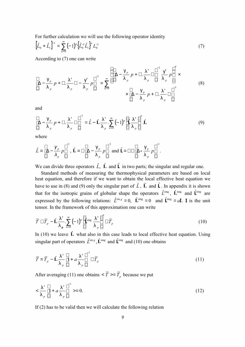
For further calculation we will use the following operator identity

[ ] ( ) ∑∞

=

−−−−=+

0

101

10

1

10ˆˆ1ˆˆ

n

nn LLLLL (7)

According to (7) one can write

∑∞

= −

−

−

∇

λλ ′

∇+λγ

−∆×

×

λγ′

∇

λλ ′

∇+λγ

−∆

=

λγ′

−∇λλ ′

∇+λγ

−∆0 1

1

1

.

.

.n

pp

p

n

ppp

p

ppp

p

p

pp

pp (8)

and

( )∑∞

=

−

λλ ′

−λλ ′

−=

∇

λλ ′

∇+λγ

−∆0

1

ˆ.ˆ1.ˆˆ.n

n

p

n

ppp

p Lp LL L (9)

where

,ˆ1−

−∆= pL

p

p

λγ

1

ˆ−

λγ

−∆∇= pp

pL and .ˆ1−

λγ

∆∇∇= pp

p-L

We can divide three operators ,L L and L in two parts; the singular and regular one.Standard methods of measuring the thermophysical parameters are based on local

heat equation, and therefore if we want to obtain the local effective heat equation wehave to use in (8) and (9) only the singular part of L , L~ and L . In appendix it is shownthat for the isotropic grains of globular shape the operators singL , singL and singL areexpressed by the following relations: ,0ˆsin =gL 0ˆ sing =L and IL a=singˆ . I is the unittensor. In the framework of this approximation one can write

( )∑∞

=

∇

λλ ′

−λλ′

−≅0

sing ~ˆ1.ˆ~~n

p

n

p

np TTT L

p

L (10)

In (10) we leave L what also in this case leads to local effective heat equation. Usingsingular part of operators singsin ˆ,ˆ LgL and singL and (10) one obtains

ppp

p TaTT ~1ˆ~~1

∇

λλ ′

+λλ ′

−=−

L (11)

After averaging (11) one obtains pTT ~~ >=< because we put

.011

>=

λλ ′

+λλ ′

<−

pp

a (12)

If (2) has to be valid then we will calculate the following relation

10

( ) ( ) ><λ−>=∇λ<−>=< TT p~~~ rrq , (13)

where we used (11). Comparing (2) and (13) we obtain .effp λ=λ It still remains for us

to determine .~ >γ< T Using (10) we can write

pp

p TaTT ~1~~~1

∇>

λλ ′

+λλ ′

γ<−>γ>=<γ<−

p

L (14)

If we substitute the singL instead L in (14) we obtain

>><γ=<>γ>=<γ< TTT p~~~ (15)

Introducing (13) and (15) into (3) one obtains

( )[ ] ><∆λ=−><>γ< TTTp eff~,0~ r (16)

or

><∆λ=∂

><∂>γ< TtT

eff (17)

Equation (17) represents the local effective heat equation.

3 Determination of >< γ and effλ

Comparing equations (3) and (16) and using effp λ=λ we obtain that .pγ>=λ< Thereis some difference between pλ and .pγ In regard to >γ=<γ p we see that >λ≠<λ p

because effλ depends on the paths of the transport of the energy.

According to assumption II. the probability that in a certain place there is located the

ith component is expressed by volume fraction VVi of the ith components. From this fact

it follows that

( )∑=

ρ>=γ<n

i

iii V

Vc1

r (18)

and

( ) .01

11

1

=λ+λ−

λ−λ>=

λλ ′

+λλ ′′

< ∑=

−n

i ieff

effii

pp aaVV

a (19)

Finally we will interpretate relation (18). The average density is expressed by therelation

11

∑ ∑= =

==ρ>=ρ<n

i

n

i

i

i

iii V

MVV

VM

c1 1

(20)

where ∑=

=n

iiMM

1

and iM is the mass of ith component. Further

∑=

=><n

iiiw wcc

1

, (21)

where MMw i

i = is the mass fraction of ith component. Introducing mass fractions into

(21) one obtains

∑=

==><n

i

i

i

iw M

QMM

MQ

c1

(22)

where Qi is the heat needful for the increase of temperature of ith component about 1K.Now we can write

∑ ∑= =

>><ρ=<=ρ>=γ<n

i

n

iw

i

i

i

i

iiii c

VV

MQ

VM

VV

c1 1

. (23)

Relation (23) is due to Assumption II.

4 Conclusion

The effective non-stationary heat equation and the formula for the effective thermalconductivity were derived.

Appendix

Operator L is defined in the following way: ( ) ( ) ( )∫ ′′′−= rrrrr dfGfL . Applying

operator

λγ

−∆ pp

p we obtain ( ) [ ] ( ) ( )∫ ′′′−−∆= λγ rrrrr dfGpf

p

p . If the last equation

has to be fulfilled then the following equation has to hold

[ ] ( ) ( )rrrr ′−δ=′−−∆ λγ Gp

p

p (24)

The solution of equation is expressed in form

( )

λ

γ−

π−= rp

rG

p

pexp141r

12

With the help of the function ( )rG the operators gLsinˆ , singL and singL are defined in the

following way: ( )∫Ω

→=

R

dGLR

defg rr

0

sin limˆ 1 ; ( )∫Ω

→∇=

R

dGR

g 1limˆ0

defsin rrL ;

( )∫Ω

→∇∇=

R

dGR

def1lim

~0

sing rrL ; where RΩ is the region of spherical shape. From the above

definitions of the singular operators one can easy prove that ,0ˆsin =gL ,0ˆ sing =L

1ˆsing IL a= , where a31= .

Acknowledgement

Authors wish to thank the Slovak Science Grant Agency for the financial support underthe contract 4256/99.

References

[1] Beran M J, 1974 Application of Statistical Theories for the Determination ofThermal, Electrical and Magnetic Properties of Heterogenous Materials. InComposite Materials, Vol.2. (New York, Academic Press) p.209

13

MEASURING THE TEMPERATURE-DEPENDENTTHERMAL CONDUCTIVITY AND HEATCAPACITY IN BUILDING MATERIALSJozefa Lukovičová, Jozef Zámečník

Department of Physics, Faculty of Civil Engineering, Slovak Technical University,Radlinského 11, SK-813 68 Bratislava, SlovakiaEmail: lukovico@svf.stuba.sk, zamecnik@svf.stuba.sk

Abstract

The method for measuring the temperature dependent thermal conductivity and heatcapacity is based on the solution of the nonlinear inverse problem of a parameteridentification. The solution of the corresponding direct problem is obtained using a timemarching boundary element method. The determination of this thermal propertiesrequires boundary and initial data and a set of temperature measurements at a singlesensor location inside the heat conducting body. The application of this method isillustrated for one dimensional heat conductivity in the building material furnance slag -based concrete.

Keywords: thermal conductivity, heat capacity, inverse problem, building materials

1 Introduction

Many theoretical and experimental methods for measuring the thermophysicalproperties are developed in the literature, they include, among others, the steady-statemethod, the probe method, the periodic heating method, the least squares method andpulse heating method. This paper deals with the method for measuring temperature-dependent thermal conductivity and heat capacity based on the inverse problem ofidentification of parameters. The method can be considered as a reasonable alternativeto the classical methods for measuring thermal properties, because for wide temperaturerange it is possible to determine thermal properties as functions of temperature.

The determination of the mater parameters from some global measurements belongsto the class of inverse problems, which are known to be ill-posed. The effectiveness ofthe inverse solution is substantially dependent on numerical realization of the directproblem’s solution and on its precision.

Theoretical studies of the identification of parameters were investigated by Cannon[1]. However, these studies, in order to make the identification heat conduction problemwell-posed, introduce strong hypotheses on the input data which are seldom satisfied inpractical experiments. Huang [2] employed a weighted finite difference method for thesolution of the direct problem as part of the inverse problem that should be modified, formixed boundary condition. Such modification is not required if the boundary elementmethod (BEM) is used. A review of BEM can be found in Brebbia [3]. Ingham [4]implemented the BEM in the direct nonlinear case of the inverse identification situation.We use modified Ingham’s idea.

14

2 Formulation of the problem

We consider the one-dimensional, nonlinear heat conduction problem in slab geometry.The dimensionless mathematical formulation of this problem can be expressed as

)),()((),()( 0 xtxTTk

xF

ttxTTC

∂∂

∂∂=

∂∂ ( , ) ( , ) ( , ]x t ∈ ×0 1 0 1 (1a)

)(),()( 0 tqx

txTTk =∂

∂− at x = 0 , t ∈ ( , ]0 1 (1b)

)(),( 1 tTtxT = at x =1, t ∈ ( , ]0 1 (1c)

)(),( 0 xTtxT = for t = 0 , x ∈ [ , ]0 1 (1d)

where T is the temperature, x

txTTkq∂

∂= ),()( is the heat flux, k T( ) is the thermal

conductivity, C T( ) is the heat capacity per unit volume, q t0 ( ) , T t1 ( ) , T x0 ( ) are knownfunctions. The temperature, distance, time, heat capacity and thermal conductivity aredimensionless with respect to Tr (a reference temperature), L (length of the slab), t f

(final time of interest during which a specific practical heat conduction experiment isperformed), Cr , and kr (reference value), respectively. The Fourier number

)/()( 20 LCtkF rfr= .

A temperature sensor is installed at an arbitrary spatial position )1,0(∈= dx andtemperature measurements T tm( ) ( ) are recorded in time, namely

T x t T tm( , ) ( )( )= at x d= , t ∈ ( , ]0 1 (2)

For the inverse problem, the thermal properties k T( ) and C T( ) are regarded as beingunknown, but everything else in equation (1) is known. The determination of k T( ) andC T( ) from boundary and initial data and temperature measurements T m( ) is needed tomake by utilizing an inverse analysis.

3 Direct problem solution

The first step of inverse analysis is to develop the corresponding direct solution for theproblem (1). A boundary element method is employed for solution of the nonlinearsystem (1) . By using the Kirchhoff transformation

∫=T

dTTkTu0

)()( (3)

denoting )),((),( txTutxu = , ]1,0[)1,0(),( ×∈tx , equations (1) in the new variableu can be written as

2

2 ),()),((),(x

txutxTat

txu∂

∂=∂

∂ , ]1,0()1,0(),( ×∈tx (4a)

))((),(0 tqu

xtxu =

∂∂− at x = 0 , ]1,0(∈t (4b)

15

))((),( 1 tTutxu = at x =1, ]1,0(∈t (4c)

))((),( 0 xTutxu = for t = 0 , x ∈ [ , ]0 1 (4d)

where

)()()( 0 TC

TkFTa = (5)

is the dimensionless thermal diffusivity.According to weighted residuals method, the residue of (4a) weighted with

fundamental solution u* and integrated over the domain produces zero

0))(( *2

2

=τ∂∂−

∂∂

∫∫ dxdutu

xuTa

Ltt f

(6)

If the thermal diffusivity a is constant, then for (4a) a fundamental solution is available

)())(4

)(exp())(4(

1),;,(2

*

21 τ−

τ−ξ−−

τ−π=τξ tH

tax

tatxu

where H is the Heaviside function and ξ and τ are generic space and time variables,respectively. In the case of non-constant thermal diffusivity the use of the fundamentalsolution (6) is accompanied by a time marching technique in which a T( ) is assumedconstant at the beginning of each time step. Therefore, starting from the initial timet0 0= , over each time element [ , ]t ti i−1 , the value of ai is taken as the mean average

∫ −==1

0 1)),(()( dxtxTaTaa ii (7)

Therefore, over each time step nonlinear partial differential equation is linearized.Applying the Gaussian reciprocity theorem, using the fundamental solution u* andapproximation (7), equation (6) is transformed into following integral equation for eachtime step [ , ]t ti i−1 , see Brebbia.[5]

∫∫−

τττ+τττ=η−

i

i

t

t i

i

i i dtxuuadtxuuatxux1

),1;,(),1(),0;,(),0(),()( *'

1

*' -

+τττ−τττ ∫∫−

i

i

i

i

t

t i

t

t i dtxuuadtxuua1

),1;,(),1(),0;,(),0( *'*'

∑ ∫=

−−−

0

111

*1 ),,,(),(

N

j

y

y iij

jdytytxutyu , ],[ 1 ii ttt −∈ , )1,0(, ∈yx (8)

where primes denote differentiation with respect to x and η( )x is a coefficient which isequal to1 for )1,0(∈x and 0.5 if 1,0∈x .

Assuming that the temperature and the heat flux are constant over each time step[ , ]t ti i−1 , the constant approximation of integral equation (8) and of equations (4b) and(4c), can be written in the form

∫∫−

ττ+ττ=η−

i

i

t

t iii

i

i iiii dtxuatudtxuatutxux1

),1;~,()~,1(),0;~,()~,0()~,()( *'

1

*' -

16

+ττ−ττ ∫∫−

i

i

i

i

t

t iii

t

t iii dtxuatudtxuatu1

),1;~,()~,1(),0;~,()~,0( *'*'

∑ ∫=

−−−

0

1111 ),,~,()~,~(

N

j

y

y iiijj

jdytytxutyu , x y, ( , )∈ 0 1 (9a)

))(()~,0( 0 ii tqutu =′− , t t ti i∈ −[ , ]1 (9b)

))~,1(()~,1( 0 ii tTutu = , t t ti i∈ −[ , ]1 (9c)

where ~ ( ) /t t ti i i= +−1 2 is midpoint of the element ii tt ,1− and 2/)(~1 jjj yyy += − for

j =1to N , are the midpoints of the elements y yj j−1 , which are used to discretise thesegment [ , ]0 1 into N elements. The integrals in (9) are calculated analytically.

For calculating temperature function u x t( , ) at any point inside the layer[ , ] [ , ]0 1 1× −t ti i it is needed to find heat flux u ti

' ( , ~ )0 , u ti' ( , ~ )1 and transformed

temperature u ti( , ~ )0 , u ti( , ~ )1 on the boundaries x = 0 and x =1, which can be obtainedby solving a system of four equations (9b,c) and (9a)- if point x tend to 0 and to 1 .Once the values of u x t( , ) are obtained, the temperature T x t( , ) is calculated byinverting the transformation (3), namely

)),((),( 1 txuutxT −= , ( , ) [ , ] [ . ]x t t ti i∈ × −0 1 1 (10)

and boundary heat fluxes are given by

q x t q x t u x ti i( , ) ( , ~ ) '( , ~ )= = x ∈ , 0 1 , t t ti i∈ −[ , ]1 (11)

In particular, the values of u y tj i( ~ , ) for j =1to N , need to be calculated in order toprovide the ‘initial’ condition at the time t i and to proceed to the next time step[ , ]t ti i+1 . Also the corresponding values of the temperature, T y tj i(~ , ) for j =1to N ,are required in order to calculate the new constant value of the thermal diffusiviy ai+1 ,given by (7) at the time t i .Based on this time marching technique the BEM providesthe values of u and C at any point in the solution domain.

4 Inverse problem

For the inverse problem, the thermal properties k(T) and C(T) are regarded as beingunknown, but everything else in equations (1) is known. In addition temperaturereadings T tm( ) ( ) taken at arbitrary spatial position x d= ∈ ( , )0 1 are consideredavailable.

For a given k(T) and C(T) (initial guesses of k(T) and C(T)) is denoted the solution of(9) by T x t C k( , ; , ) and the solution at x d= , T tc( ) ( ) . The solution of the presentinverse problem is to be obtained in such a way that the least-squares normT Tc m( ) ( )−

2 is minimized. In practice, only a finite set of time measurements may be

available at some discrete times, t i' , namely

T d t T t Tim

i im( , ) ( )' ( ) ' ( )= = , i =1to M (12)

17

Requiring that the continuous functions k(T) and C(T) be determined from only a finiteset of data (12) results in a non-unique solution problem. In order to be able to achieve aunique solution, the unknown functions k(T) and C(T) are parameterized. Theparameterization is performed by assuming that the k(T) and C(T) are taken as a set ofpolynomials,

C T C Tjj

j

R

( ) = −

=∑ 1

1and k T k Tj

j

j

R

( ) = −

=∑ 1

1(13)

Then the least-squares norm in discretised form becomes

S C k T T C kim

ic

i

M

( , ) [ ( , )]( ) ( )= −=∑ 2

1(14)

where C C j= ( ) and k k j= ( ) , for j =1to R , are the unknown vectors of the thermal

conductivity and heat capacity, and T C kic( ) ( , ) is the calculated value of the temperature

at t t i= ′ , for i =1to M , obtained from the BEM solution of the direct problem (9), byusing the estimated values of the ( , )C k . The unknown parameters k j and C j are thendetermined as the solution of the minimization nonlinear least-squares norm (13) usingthe Newton -Raphson method, by the package LSODA[6].

Temperature dependent uniqueness conditions applicable to the problem ofestimating C T( ) and k T( ) are very difficult, see Cannon [1] and as simple alternative,in order to be able to obtain a unique solution, C T( ) and k T( ) are fixed at some points.The stability oft the solution is ensured since the number of independent parameterswhich are to be estimated is, in general, small and no further regularization terms isneeded.

6 Experimental results

The experiments were performed on the furnace-slag-based concrete. The measuredsample is an alloy geometry of length L = 0 2. m , with reference thermal conductivitykr W / mK= −10 1 , heat capacity Cr

3J / m K=106 , temperature T T Tro C= − =max 0 180

and is subject to a heat transfer experiment with q t T0 0 2( ) .= and T t T1 0 20 180( ) /= =over a period of time t f = ×36 103. s , the Fourier number F0 0 9= . . The heat flux q t0 ( )

is known at a prescribed rate of ∆ ∆t t tf* = , temperature T m( ) is recorded at sampling

rate of ∆t t Mf'* /= .

The inverse determination of the heat capacity and the thermal conductivity startinginitially with the guesses:

2321)( TCTCCTC ++= and k T k k T k T( ) = + +1 2 3

2

where C1 1= , C2 0 75= . , C3 125= . , k2 4= , k3 4 75= .For the time step ∆t = 0 01. and number of measurements M = 60, numericaldimensionless results are obtained as follows:

C T T T( ) . . .= + +13 0 203 0 6015 2 and k T T T( ) . . .= + +3 4 11821 3 4521 2

18

Real physical values are shown on Fig.1

Fig 1 Thermal conductivity and heat capacity as a function of temperature

Precise tests of accuracy and stability of the method as well as the sensitivity to theexperimental errors are tested by Lukovičová and Zámečník in [7].

7 Conclusion

The presented method for simultaneous determining the thermal conductivity and heatcapacity as a function of temperature is found by means of the solution of an inverseheat conduction problem. The method is suited for practical calculating of thermalproperties of porous materials and for analyzing of heat conduction measurementproblems.

Acknowledgment

Authors are grateful to VEGA (Grant No.1/4063/79) for financial support of this work.

References

[1] Cannon J R, 1964 Determination of certain parameters in heat conductionproblems, J. Math. Anal. Appl. 8, 188-201

[2] Huang C H, Yan J Y, 1995 An inverse problem in simultaneously measuringtemperature-dependent thermal conductivity and heat capacity, Int. J. Heat MassTransfer 38, 3433-3441

[3] Brebbia C A, 1984 Application of the boundary element method for heat transferproblems, in Proc.Conf. Model et Simulation en Thermique (Poitiers:Ensma) p.1

[4] Ingham D B, Yuan Y, 1993 The solution of nonlinear inverse problem in heattransfer, IMA J. Appl. Math. 50, 113-132

[5] Brebbia C A, Telles J C F, Wrobel L C, 1984 Boundary element Techniques:Theory and Application in Engineering, (Berlin: Springer-Verlag)

[6] Constales D, Automatic differentiation in lsoda. In preparation[7] Lukovičová J, Zámečník J, 1999 Determinination of thermophysical coefficients in

nonlinear heat conducting porous material, Slovak J. Civil Eng., In preparation

19

THE LINEAR THERMAL EXPANSION OFBUILDING MATERIALS AT HIGHTEMPERATURESJan Toman1, Robert Černý2

1 Department of Physics, Faculty of Civil Engineering, Czech Technical University,Thákurova 7, 166 29 Prague 6, Czech Republic2 Department of Structural Mechanics, Faculty of Civil Engineering, CzechTechnical University, Thákurova 7, 166 29 Prague 6, Czech RepublicEmail: toman@fsv.cvut.cz, cernyr@fsv.cvut.cz

Abstract

A method for measuring linear thermal expansion of porous materials in the hightemperature range up to 1000oC is introduced in the paper. The measuring device isbased on the application of a comparative technique. A bar sample of the studiedmaterial is put into a cylindrical, vertically oriented electric furnace. As it is technicallydifficult to perform length measurements directly in the furnace, a thin ceramic rod,which passes through the furnace cover is fixed on the top side of the measured sample.The length changes can be determined outside the furnace in this way provided themeasurement is performed at the same time on the sample of a standard material.A practical application of the method is demonstrated with two types of common porousbuilding materials, cement mortar and refractory concrete.

Key words: thermal expansion, high temperatures, building materials

1 Introduction

Thermal expansion of solid materials is measured by commercially produceddilatometers mostly. Various treatments are employed, for instance the methods basedon variations of electric resistance, capacity, inductance or the interference methods (seefor instance [1-3] for details). Among most commonly used laboratory devices formeasuring thermal dilatation of bar solid samples belong Edelmann dilatometer andvarious comparators.

The most of the mentioned methods are suitable for relatively small samples,typically up to 10 mm in standard experimental setups. For this reason, they can beapplied for measuring metals, glass, various polymers and other materials which arehomogeneous in this length scale, but for porous building materials with characteristicdimensions of nonhomogeneities as high as several mm or cm are they practicallyinapplicable. Therefore, some modifications of standard treatments are necessary inorder to achieve a sufficient accuracy in measuring thermal expansion of thesematerials.

Two examples of such modifications are described in [4]. The first of them is basedon the application of a contact comparator, the second one employs an opticalcomparative treatment and consists in measuring the positions of microtargets on thesamples through the window of the climatizing chamber using cathetometric reading.

20

Both methods are supposed to measure linear thermal expansion coeffiient in thetemperature range of -50oC to 200oC.

In this paper we introduce a method for measuring linear thermal expansion ofporous building materials in the high temperature range, up to 1000oC in the currentexperimental setup.

2 Theoretical relations

The infinitesimal change of length due to the change of temperature is defined by

dTldl α= 0 , (1)

where lo is the length at the reference temperature To, α is the linear thermal expansioncoefficient.

From (1) it follows that

dTdl

l0

1=α ; (2)

and is generally a function of temperature, α = α(T). Assuming lo = const. we obtainanother useful relation from Eq. (2),

dTd

dTlld

ε=

=α 0 , (3)

where ε is the relative elongation, ε = ε (T).Integrating (3) we arrive at

∫ ττα=εT

T

dT0

)()( . (4)

In small temperature intervals, where T → To we can assume

.0 const=α=α , (5)

00 TT −

ε=α , (6)

and αo can be calculated from a single experiment consisting in heating the sample fromthe initial temperature To to the final temperature T and measuring the relativeelongation ε.

In wider temperature ranges, the assumption (5) is no longer valid, and we have toemploy the general definition relation (3). We choose a reference temperature To, heatthe samples to the temperatures Ti, i = 1,...,n covering the desired temperature range anddetermine the corresponding values εi; i = 1,...,n. The pointwise given function εi = f(Ti)is then approximated using a regression analysis and its continuous representation ε (T)is obtained. Finally, the linear thermal expansion coefficient α(T) is calculated using (3)as the first derivative of the ε(T) function with respect to temperature.

21

3 Experimental setup

The measuring device for determining the linear thermal expansion of porous materialsin high temperature range is based on the application of a comparative technique. A barsample of the studied material is put into a cylindrical, vertically oriented electricfurnace. As it is technically difficult to perform length measurements directly in thefurnace, a thin ceramic rod, which passes through the furnace cover, is fixed on the topside of the measured sample. The length changes can be determined outside the furnacein this way, for instance by a dial indicator, but on the other hand, the temperature fieldin the ceramic rod is very badly defined, and it is not possible to determine directly,which part of the total change of length is due to the measured sample and due to theceramic rod.

Therefore, the measurement is performed at the same time on the sample of astandard material (such as copper or iron where the α(T) function is known) which isput into the furnace together with the studied material and is provided with an identicalceramic rod passing through the cover. The change of length of the ceramic rod can bedetermined in this way, and consequently also the length change of the measuredsample.

It should be noted that temperature field is not constant in the whole volume of thefurnace due to the differences of heat loss in the heated walls and in the cover.Therefore, temperature field in the furnace is measured by thermocouples, and anaverage value of temperature is considered in the α calculations.

4 Practical application

A practical measurement of the linear thermal expansion coefficient of a porousmaterial on the device proposed in the previous Section can be described as follows.The measured sample and the standard are put into the furnace, provided by the contactceramic rods, and the initial reading on the dial indicators is performed. Then, the powerof the electric heating is adjusted for the desired temperature Ti in the furnace using aregulating transformer, and the length changes are monitored on the dial indicators.After the steady state is achieved, i.e. no temperature changes in the furnace and nolength changes of both measured sample and the standard are observed, the finalreadings of length changes are done. The length change of the measured sample iscalculated from the formula

∫ ττα+∆−∆=∆iT

Tsisimi dlTlTlTl

0

)()()()( so, (7)

where ∆lm, ∆ls are the final readings of total length changes of the studied material andof the standard including the length changes of the ceramic rods, respectively, lo,s is theinitial length of the standard, αs is the known linear thermal expansion coefficient of thestandard, and the corresponding value of relative elongation can be expressed in theform

mo,

)()(

lTl

T ii

∆=ε , (8)

where lo,m is the initial length of the measured sample.

22

Fig 1 The dependence of the temperature in the furnace on timeFig 2 The dependence of the elongation of iron and refractory concrete on time

The measurements are then repeated with other chosen values of furnacetemperatures Ti, and the calculation of the α(T) function of the measured material isperformed as explained in Section 2.

5 Experimental results

At first, a series of experimental measurements was performed to verify the designedmethod. Not only parameters of temperature and length changes, but also timedependencies of these quantities were studied. Examples of these dependencies areshown in Figs 1,2. The time necessary for the stabilization of the measuring device canbe identified from these figures. In the case of T = 700oC it was approximately 4 hours.

Then, set of comparative experiments on one hand with two samples of the samematerial, and on the other hand with two different standard materials was done. Fig 3shows a comparison of length changes of two cylindrical iron bars with two differentdiameters in dependence on temperature. Apparently, the length changes of bothsamples are very close each other, the maximum difference being 2%.

In the second part of our measurements we have performed experiments with thesamples of two different types of porous building materials, cement mortar andrefractory concrete. While cement mortar is designed for using in normal temperatureconditions, the refractory concrete is supposed to be used in blast furnaces, andtherefore it should have not only high temperature resistance, but also low thermalexpansion coefficient in wide temperature range.

Fig 4 shows that the changes of linear thermal expansion coefficient of cementmortar with temperature are in a reasonable range only up to ~ 200oC, then a dramaticcourse of the α(T) function with a maximum at ~ 500oC followed by a fast decrease canbe observed. Apparently, the samples of cement mortar do not resist to hightemperatures very much. Structural changes and chemical reactions take place in thematerial if the temperatures grow higher than to ~ 200oC, and the original structure isdamaged. On the other hand, the refractory concrete was proved to be a suitablematerial for its designed application. Fig 5 shows that its linear thermal expansion

23

Fig 3 The dependence of the elongation of two iron samples with the differentdiameters d on temperature

Fig 4 The dependence of the linear thermal expansion coefficient of cementmortar on temperature

coefficient is significantly lower than for cement mortar already in the lowertemperature range, and the increase of with temperature is relatively very slow.

6 Conclusions

A simple comparative method for measuring high temperature linear thermal expansioncoefficient of porous materials which is suitable for application with relatively largesamples up to 120 mm long was designed. A basic verification of the proper functionand reliability of the method was done by the measurements with standard materialswith the known α(T) functions. The practical measurements on cement mortar andrefractory concrete have shown a good practical applicability of the proposed methodwhich is significantly cheaper compared to the available commercial devices. Themethod can provide useful information for example in the design of building structuresfrom the point of view of the fire security.

Acknowledgement

This paper is based upon work supported by the Grant Agency of the Czech Republic,under grants # 103/97/0094 and 103/97/K003.

24

Fig 5 The dependence of the linear thermal expansion coefficientof refractory concrete on temperature

References

[1] Brož J et al, 1983 Fundamentals of Physical Measurements (in Czech, Prague:SPN)

[2] Gobrecht H et al, 1990 Bergman-Schaefer Lehrbuch der Experimentalphysik,Band I, 10th Edition (New York: Walter de Gruyter)

[3] Horák J, 1958 Practical Physics (in Czech, Prague: SNTL)[4] Toman J, Černý R, 1996 Coupled Thermal and Moisture Expansion of Porous

Materials, Int. J. Thermophysics 17, 271-277

25

MEASUREMENT OF THERMOPHYSICALPROPERTIES OF MATERIALS BY THE DYNAMICPLANE SOURCE METHODGabriela Labudová

Department of Physics, Faculty of Natural Sciences, Constantine the PhilosopherUniversity, Tr. A. Hlinku 1, SK-94974 Nitra, SlovakiaEmail: glabudova@ukf.sk

Abstract

The paper deals with the measurement of effusivity of materials using the dynamicplane source (DPS) method. The measurement of effusivity has been performed on airat room temperature on samples made from organic glass.

Key words: dynamic plane source method, adiabatic and isothermal conditions,effusivity

1 Introduction

Nowadays a lot of measuring methods for measurement thermophysical properties ofmaterials have appeared in literature. Among others the dynamic plane source method(DPS) based on using an ideal plane sensor (PS). The PS sensor acts both as heat sourceand temperature detector. The dynamic plane source method is arranged for a one–dimensional heat flow into a finite sample. The outer (rear) surface of the sample is incontact with a poor heat conducting material so that the boundary condition of thesample is close to being adiabatic. In particular, the adiabatic method appears to beuseful especially for measurement of materials with thermal conductivity in the range2<λ<200 W.m-1.K-1. The experimental arrangement is modified by exchanging theinsulating material on the rear surface of the sample with a very good heat conductingmaterial (heat sink) which makes the measurement possible also for samples withλ≤2 W.m-1.K-1. The presence of the heat sink on the rear surface of the sample makesthat the heat conduction process through the sample after a defined time periodapproaches the steady – state condition. The adiabatic and the isothermal method giveeffusivity of materials, which includes information about thermal conductivity andthermal diffusivity of investigated material.

2 Theory

The theory considers ideal experimental conditions - the ideal heater (negligiblethickness and mass), perfect thermal contact between PS sensor and the sample, zerothermal resistance between the sample and the material surrounding the sample, zeroheat losses from the lateral surfaces of the sample [1].

If q is the total output of power per unit area dissipated by the heater, then thetemperature increase as a function of time is given by [2]

26

( )

λ=

taxtaq

txT2

ierf2, , (1)

where a is the thermal diffusivity, λ the thermal conductivity of the sample and ierfc theerror function [3].

We consider the PS sensor, which is placed between two identical samples havingthe same cross section as the sensor in the plane x = 0. The temperature increase in thesample as a function of time conforms

( ) taqtTπλ

=,0 , (2)

which corresponds to the linear heat flow into an infinite medium [3,4]. The slope of thegraph of ∆T(t) against t gives the effusivity of the sample [5]

λρ=λ= ca

e (3)

The real experiment can contribute to the deviation of the experimental curve fromthe ideal one [6]. Some of the distortions can be eliminated by the proper choice of theevaluation time interval while the others require further modifications of Eq. (1).

3 Experimental arrangement

Between two identical samples which forms a disk with the diameter of 3.10-2 m the PSsensor having the same cross section as the samples is placed. The sensor is made of aNi – foil, 23 µm thick protected from both sides by an insulating layer made of kaptonof 25 µm thick (Institute of Physics, SAS Bratislava). The sensor acts both as heatsource and temperature detector, so the experimental arrangement is considerablysimplified (Fig. 1) [7]. Providing adiabatic DPS method we have used polyurethanefoam as a relatively good heat insulator for the sample, as the adjacent material andproviding isothermal DPS method the samples were connected to a thermal sink, weremade of Al blocks. The effusivity of the samples is obtained from the time history of thetemperature rise of the sensor during an application of the electrical current. Thetemperature changes of the sensor result in changes of its resistance and, hence thevoltage ∆U(t) across it accords to

( ) ( )tTRItU ∆=∆ α00 (4)

Here I0 is the current flowing through the PS sensor since t = 0 s, R0 is the initialresistance of the PS sensor and α is the temperature coefficient of resistivity of thenickel the PS sensor consists from.

27

Fig. 1. The experimental setup (1 – PS sensor, 2 – samples,3 – current source, 4 – milivoltmeter)

4 Results and discussion

The adiabatic and the isothermal DPS method has been tested on the samples of organicglass. The measurement of the effusivity has been performed on air at roomtemperature. The resistance of the Ni – heating element was about 1,221 Ω and thetemperature coefficient of resistivity of the heater was 0,0047 K-1. The effusivity of thesample was obtained from the slope of the graph ∆T(t) against t according to the Eq.(2). The experimental garphics were compared with the theoretical graphics and weinvestigated that for short time are this graphics identical, in Fig. 2. a), b) .

Fig. 2 Experimental (T) and theoretical (Y) dependence of the temperature increase∆T(t) as a function of the time, a) adiabatic method, b) isothermal method.

The results of the measurements are presented in Table 1. The values are the meanvalues of ten independent measurements on several organic glass samples.

From the comparison of the experimental results and the effusivity, which iscalculated from the thermal conductivity and the thermal diffusivity of the material fromtabular data we can see that both adiabatic and isothermal DPS method give very closeresults.

0.0

0.5

1.0

1.5

2.0

0 30 60 90 120 150

t [ s ]

T [ K

]

T

Y

0.0

0.2

0.4

0.6

0.8

1.0

1.2

0 30 60 90 120 150

t [ s ]

T [ K ]

T

Y

28

Table 1. Experimental results (L - the sample length, e1 (e2) - the effusivity obtainedfrom adiabatic (isothermal) DPS method, e3 - the effusivity calculated fromtabular data of thermal conductivity and thermal diffusivity , I - the current,diff e1 (e3), diff e2(e3) – the difference between the measured and calculatedeffusivities).

Mate-rial

Lm

e1Ws1/2m-2K-1

e2Ws1/2m-2K-1

IA

e3

Ws1/2m-2K-1

diff e1(e3)%

diff e2(e3)%

Org. glass 10-2 568.8

+/-3.0571.1+/-3.7 0.267 570.73 0.333 0.061

Acknowledgement

Author wishes to thank the Slovak Science Grant Agency and the ministry of Educationfor the financial support under the contracts 1/6115/99 and Gr/Sl/L80.

References

[1] Karawacki E, Suleiman, B M, ul-Hag I, Nhi B T, 1992 An extension to theDynamic Plane Source Technique for Measuring Thermal Conductivity, ThermalDiffusivity and Specific Heat of Dielectric Solids, Rev. Sci. Instrum., 63, 4390-4397

[2] Beck J V, Arnold K J, Parameter Estimation in Engineering and Science, (NewYork, John Wiley and Sons) p.448

[3] Carslaw H S., Jaeger J C, 1959 Conduction of Heat in Solids, (Oxford, ClarendonPress)

[4] Karawacki E, Suleiman B M, 1991 Dynamic Plane-Source Technique for the Studyof the Thermal Transport Properties of Solids, High Temp. High Press. 23, 215-223

[5] Kubičár L, Boháč V, 1997 Review of Several Dynamic Methods of MeasuringThermophysical Parameters, in Thermal Conductivity 24, (Pittsburgh, TechnomicPublication Company, Inc.) p.135

[6] Kubičár L, 1990 Pulse Method of Measuring Basic Thermophysical Parameters,Comprehensive Analytical Chemistry, Vol XII, Thermal Analysis, Part E, (Ed:Svehla G, Amsterdam, Oxford, New York, Tokyo, Elsevier )

[7] Labudová G, Malinarič S, Vozár L, 1999 A Simple Apparatus for Measurement ofThermophysical Properties of Composites, in Proceedings of the 9th Joint SeminarDevelopment of Materials Science in Research and Education, (Bratislava, STU )p.46

29

AN ACCURACY OF MEASUREMENT THETHERMAL DIFFUSIVITY OF TWO-LAYEREDCOMPOSITELibor Vozár1, Wolfgang Hohenauer2

1 Department of Physics, Faculty of Natural Sciences, Constantine the PhilosopherUniversity, Tr. A. Hlinku 1, SK-94974 Nitra, Slovakia2 Department of Materials Technology, Austrian Research Centers, A-2444 Seibersdorf,AustriaEmail: vozar@uvt.uniag.sk, wolfgang.hohenauer@arcs.ac.at

Abstract

The paper deals with an investigation of two-layered systems using the laser flashmethod. The attention is dedicated to the study of the composites with the ideal thermalcontact stated by zero thermal contact resistance.

It is well known that an estimation of the thermal diffusivity of a layer in a compositerequires besides the knowledge of other relevant properties to know the thermaldiffusivity of the remained layer. The inaccuracy of this ‘known’ thermal diffusivitysignificantly influences the accuracy of the unknown thermal diffusivity estimation. Thepaper summarizes the performed simulations that indicate error propagation and it guessthe accuracy and measurement limits on an ideal two-layered system.

Key words: layered structures, thermal diffusivity, thermal contact resistance, flashmethod

1 Introduction

An application of various composites, especially ‚two-layered‘ coatings on substrates,has increased in a number of applications, such as thermal barriers, emissivity controls,electric insulation and wear, and erosion and corrosion resistance protection. Becausesuch systems are being utilized under different thermal conditions, the knowledge oftheir thermophysical properties is of a great importance. In situ measurement on layeredsystems allow to test how thermophysical properties (the thermal conductivity and thethermal diffusivity) of components differ from those values received for bulk materials.

Determination of the thermal diffusivity of a component on a two-layered compositeusing the flash method can be viewed as a dependent measurement [1]. An estimation ofthe thermal diffusivity of one layer besides the knowledge of other relevant properties(the density, the heat capacity and the thickness of components) requires to know thethermal diffusivity of the remained layer. Errors in measurement of these ‘additional’parameters are propagated through the data reduction and result as inaccuracy of thethermal diffusivity determination. This phenomenon influences the measurement limitsthat exist for an experimental apparatus and sample dimensions also in the case ofmeasurement of homogeneous materials.

This paper presents results of the study of the influence of the inaccuracy of the‘known’ thermal diffusivity to the accuracy of the unknown thermal diffusivity

30

estimation. The methodology proposed in [1] is here applied to copper/alumina basedtwo-layered systems.

2 The flash method

In the flash method, the front face of a disk-shaped sample is subjected to a pulse ofradiant energy coming from a laser [2]. If material boundaries are flat and parallel to thesample front and rear surfaces and if there are no heat losses from the radial surfaceone-dimensional heat transfer occurs across the sample. Analyzing the resultingtemperature rise on the opposite (rear) face of the sample any thermophysical propertyvalue (thermal diffusivity of one layer, or the thermal contact resistance) can becomputed [3,4].

2.1 Theory

The analytical model assumes one-dimensional heat flow through the two-layeredsample that consists of two layers of thickness e1 and e2. We consider a good thermalcontact between the layers stated by zero thermal contact resistance. We assume to haveuniform and constant thermal properties and densities of both layers and that the frontface (at x=-e1) is uniformly subjected to the instantaneous heat pulse with the heat Qsupplied to the unit area. In case of non-ideal experimental conditions - when heatlosses from the front and rear face should be taken into account, appropriate boundaryconditions include heat flux terms with the heat transfer coefficients h1 and h2. Theexpression for the transient temperature rise at the sample rear face (x=-e2) can bewritten in the non-dimensional normalized form [5,1] as

∑∞

=∞ +

ηω

γ−+==θ

1k 0

22

21

2kexp

)1(2)()(edd

t

PUT

tTt . (1)

Here T∞ is the adiabatic limit temperature – the temperature the sample would havereceived under ideal adiabatic conditions

222111 ececQT

ρ+ρ=∞ .

Here ρ is the density, c the heat capacity and

2

22 a

e=η ,

with a the thermal diffusivity and

)cos()cos( kk0 γ+γ= UPUd

[ ] [ ]

[ ] [ ] )cos()cos()sin()sin(2

)cos()cos()sin()sin(

kkkkk3k

21

k2k12k

1k2k1

k

1

γ−γγ−γ−γγω+

+γ+γγω+γ+γ

γω=

UPUUPZ

UPYYUPUYYde

!

!

and γk is the kth positive root of

31

[ ] 0)sin()sin()cos()cos()sin()sin( 121

1 =

γ−γγω+γ+γ

γω−γ+γ PZUPYYUP

The definition of other parameters is written in the Appendix.

2.2 Data reduction

An original software package for experimental ‘flash method’ data processing has beendeveloped [6]. The software currently allows studying of two-layered materials withzero or non-zero thermal contact resistance, respectively, as well as three-layeredmaterials with the ideal thermal contact (uniform - zero thermal contact resistance). Theapplied theory considers either the ideal adiabatic boundary conditions or heat lossescan be taken into account, respectively.

The data reduction consists of a least-squares-fitting the measured temperature risevs. time evolution. Because we have semi-linear fitting tasks - working expressionslinearly depend on the normalization factor - adiabatic limit temperature T∞, thealgorithm described elsewhere [7,8] that shifts the fitting to solving a set of algebraicequations has been reliable implemented.

Results of sensitivity analysis in the case of the presented ideal two-layeredcomposite show that normalized sensitivity to front layer diffusivity a1 and sensitivity torear layer diffusivity a2 vs. time curves are close to being linearly dependent. Thisindicates that these parameters can’t be estimated simultaneously in a simple flashmethod experiment [6]. The sensitivity to Biot number Bi and the temperature rise curvethat is equal to the sensitivity to the adiabatic limit temperature T∞ and sensitivity to rearlayer diffusivity have different shape. This facts confirm that a simultaneous uniqueestimation of the adiabatic limit temperature T∞, of the Biot number Bi and one of thethermal diffusivities a1 and a2, respectively, can be performed successfully.

2 Accuracy limits

In order to investigate conditions for the thermal diffusivity determination and accuracylimits the following analyses were performed. We took the two-layered model andcalculated various simulated temperature rise vs. time curves. We assumed to havecopper and alumina two-layered composite with their relevant (bulk) properties and weconsidered random heat losses at the level that corresponds to a real laser flashexperiment. We calculated simulated temperature rise vs. time curves for variousthickness ratios eCu/(eCu+ealumina) while we considered the total thickness e=eCu+ealuminato have constant. We analyzed how is an estimation of the thermal diffusivity of onelayer sensitive to inaccuracy of knowledge the second layer thermal diffusivity. Fig 1presents results of an estimation of the thermal diffusivity of alumina when the thermaldiffusivity of the supplementary component - copper changes in a range of ±1-3%. Wesee that the accuracy of the determination of the thermal diffusivity of alumina increaseswhen its thickness (ealumina) increases. Similar results can be received for the thermaldiffusivity of copper estimation which result varies as a result of deviation of aluminathermal diffusivity. Difference consists in fact, that the accuracy of the determination ofthe thermal diffusivity of the poorer thermal conductive material (alumina) is muchhigher that the determination of the higher conductive component. [1].

32

Fig 1 Variation of the thermal diffusivity of alumina vs. thickness ratio caused bydeviations of the thermal diffusivity of copper (±3%)

If one performs similar analyses for different component thermal diffusivities ratiosthe following quantitative relations between the accuracy of the thermal diffusivityestimation and layers thickness ratio can be received. Fig 1 shows that in case the errorin the copper thermal diffusivity is less than 3% (2% or 1%, respectively) the accuracyof the thermal diffusivity of alumina estimation better than 1% can be achieved onlywhen the condition eCu/(eCu+ealumina)<0.67 (0.74 or 0.82, respectively) is fulfilled.The choice of the alumina estimation accuracy (1%) we considered is influenced by thefact, that we have not assumed any other disturbing phenomena, as for instance arandom noise that can increase the inaccuracy of the measurement to a usual level.Performing similar analyses for different thermal diffusivity ratios, the accuracy limitcurves for an estimation of alumina- or copper-like material could be calculated asillustrated in Fig 2 and 3.

Here we note that all the achieved results could be generalized only with a great care.In our analyses, we have not considered variation of the density and the heat capacity.Because of a strong correlation between the thermal diffusivity and the heat capacity -density product in a layered model [8] the achieved accuracy limit curves should beslightly modified. Although any other disturbing phenomena were not taken intoaccount, the achieved results are suitable basis for predetermination of real estimationaccuracy limits.

5 Conclusion

The paper shows connection between the inaccuracy of the thermal diffusivities ofcomponents on an ideal two-layered composite and their layer-thickness- and thermal-diffusivity-ratios. The proposed approach gives a possibility to relate quantitatively theaccuracy of the thermal diffusivity estimation of one layer on a layered composite.Although there were not taken into account other disturbing phenomena (variation ofthe density and the heat capacity, noise, etc.) the achieved results give suitable basis forpredetermination of real estimation accuracy limits.

-2

-1

0

1

2

0 0.2 0.4 0.6 0.8 1

eCu/(eCu+ealum)

δa a

lum/a

alum

a Cu1.01*a Cu1.02*a Cu1.03*a Cu0.99*a Cu0.98*a Cu0.97*a Cu

33

Fig 2 Accuracy limit curves of the thermal diffusivity of alumina estimation as a func-tion of the thermal diffusivity ratios and thermal diffusivity of copper variation (±1-3%)

Fig 3 Accuracy limit curves of the thermal diffusivity of copper estimation as a functionof the thermal diffusivity ratios and thermal diffusivity of alumina variation (±1-3%)

Appendix

Parameters in the text are defined as follows

Hi= A ρi ci ei

i

ii a

e=η

where A is the cross-sectional area of the sample and

Hi/j = Hi/Hj

η2/1=η2/η1

X1=H1/2 η2/1+1

X2=H1/2 η2/1-1

ω1= η1/2+1

ω2= η1/2-1

1

2

XX

P =

1

2

ωω

=U

iii

iii ρ

=caehBi

2

12/1 Bi

BiBi =

+

η= 1

2/1

2/121

BiBiY

−

η= 1

2/1

2/122

BiBiY

2/1

2/122 η

=Bi

BiZ

Acknowledgement

Authors wish to thank the Slovak Science Grant Agency and the Hertha FirnbergFoundation of the ARCS for their financial support.

0

0.2

0.4

0.6

0.8

1

0 5 10 15

aCu/aalum

e Cu/(

e Cu+

e alu

m)

δ3%δ2%δ1%

0

0.1

0.2

0.3

0.4

0.5

0 5 10 15

aCu/aalum

e Cu/(

e Cu+

e alu

m)

δ1%

δ2%

δ3%

34

References

[1] Hohenauer W, Vozár L, An Estimation of Thermophysical Properties of LayeredMaterials using the Laser Flash Method, High Temp. High Press. (accepted)

[2] Parker W J, Jenkins R J, Butler C P and Abbott G L, 1961 Flash Method ofDetermining Thermal Diffusivity, Heat Capacity and Thermal Conductivity,J. Appl. Phys. 32, 1679-1684

[3] Balageas D L, 1989 Thermal Diffusivity Measurement by Pulsed Methods, HighTemp. - High Press. 21, 85-96

[4] Maglić K D, Taylor R E, 1992 The Apparatus for Thermal DiffusivityMeasurement by the Laser Pulse Method, in Compendium of ThermophysicalProperty Measurement Methods Vol.2 Recommended Measurement Techniques andPractices, Eds K D Maglić, A Cezairliyan, V E Peletsky (New York: PlenumPublishing Corp.) p.281

[5] Sweet J N, 1989 in Thermal Conductivity 20 Ed D P H Hasselman, J R Thomas, Jr.(New-York: Plenum) pp. 287-304

[6] Vozár L, 1999 Measurement of the Thermal Diffusivity and the Contact ThermalResistance of Two- and Three-Layered Composite Materials Using the FlashMethod, Progress report ARC Seibersdorf, CPU Nitra

[7] Gembarovič, J., Vozár, L., Majerník, V., 1990 Using the Least Squares Method forData Reduction in the Flash Method, Int. J. Heat Mass Transfer 33 1563-1565

[8] Vozár, L., Šrámková, T., 1997 Two data Reduction Methods for Evaluation ofThermal Diffusivity from Step Heating Measurements, Int. J. Heat Mass Transfer40 1647-1656

[9] Koski J A, 1985 in Thermal Conductivity 18, Ed T Ashworth, D R Smith (New-York: Plenum) pp. 525-536

35

STEADY-STATE THERMAL CONDUCTIVITYDETERMINATION OF NON-METALLICMATERIALS AT CONSTANT SURFACE HEATSOURCEPeter Matiašovský, Oľga Koronthályová

Department of Building Physics, Institute of Construction and Architecture, SlovakAcademy of Sciences, Dúbravská cesta 9, 842 20 Bratislavausarmat@savba.sk, usarkoro@savba.sk

Abstract

In determination of thermal conductivity generally the important problem is to realizesatisfactorily defined conditions on the boundaries of a specimen. A possible solution isto realize steady-state boundary conditions of 3rd kind defining heat transfer coefficientbetween specimen and measuring device. Determination of thermal conductivity is thenpossible from analytical solution of Laplace equation for the case of three-dimensionalbody heated by square surface heat source. The thermal conductivity is calculated frommeasured data on heat flow and temperature difference.

Key words: building materials, thermal conductivity, stationary measuring methods

1 Introduction

Porous building materials are characterised by densities in the range 20 - 2 500 kg/m3

and thermal conductivities in the range 0.03 - 1.5 W/m.K. Commonly used methods ofthermal conductivity determination for porous building materials are plate methods andprobe methods. Each type of the methods has its own merits and insufficiencies. Platemethods require relatively long measuring times, large specimens and ideal thermalcontact mainly in the case of thin highly conductive specimens. Probe methods arequick but they are not able to evaluate heterogeneous materials and they require idealthermal contact between specimen and probe too. For practical use a simple and quickmeasuring method should have following properties: satisfactorily large contact area, nolimitations regarding the specimen dimensions and shape, no problems with realizationof thermal contact. A possible solution is method based on steady state heating ofspecimen surface by constant heat flow with defined square thermal contact area andheat transfer coefficient. Measuring device providing these conditions have beendeveloped and tested.

36

2 Theory

We consider infinite homogeneous plate of thickness H. At a surface of the plate aconstant heat source of square area is placed. Temperature of environment is ta (Fig. 1).The thermal conductivity of the plate is detemined from analytical steady-state solutionof the Laplace equation. The mathematical formulation of the problem is given byfollowing equations:Laplace equation:

0zt

yt

xt

2

2

2

2

2

2

=∂∂+

∂∂+

∂∂ (1)

Temperature of the contact face of square heat source:

t = t for 0 <| x|<L2

and 0 <| y|B2

i ≤ (2)

Temperature of the environment:

t = t for L2

| x| and B2

| y|a < ≤ ∞ < ≤ ∞ (3)

Temperature of the opposite non-heated surface:

t = t e (4)

Boundary conditions of 2nd kind at the surfaces perpendicular to the heated one areprovided by sufficiently large x1, y1. If the dimensions of the plate are higher than x1, y1the problem can be applied for the body of finite dimensions: rectangularparallellepiped, finite cylinder, etc.

0nt

=∂∂

(5)

Boundary conditions of 3rd kind at the surface with the heat source:

[ ]z y,0)F(x, y,0)F(x,-y)t(x,

∂∂⋅λ−=⋅α (6)

The solution of the steady state problem for heat flow into the plate [1] is:

( ) ),,FUNK(ttL tL=Q aia τηρ⋅−⋅⋅λ+

αλ+

−⋅⋅λH

te (7)

( )w4

w40n 0i

3

e1we12

18=FUNK

⋅ρ⋅µ⋅π⋅−

⋅ρ⋅µ⋅π⋅−

∞

=

∞

=

+⋅−+µ⋅π⋅τ⋅

⋅⋅µπµπµπ

τηρ ∑∑ 22 i)i..sin(

n)n..sin(),,( (8)

where:

37

w ni

= +η

(9)

BL=η (10)

L and B are dimensions of the square heat source [m]

11 y2B

x2L

⋅=

⋅=µ (11)

x1, y1 are dimensions of the sample in the plane of the heat source [m]

BH=ρ (12)

H is thickness of the sample [m]

B⋅αλ=τ (13)

λ is thermal conductivity of the sample [W/m.K], α is heat transfer coefficient betweenthe source and the sample and between the sample and its surroundings [W/m2.K]. Thedefined constant value of heat transfer coefficient over the whole exposed surface areais provided by construction of the measuring device.

Thermal conductivity of the specimen is calculated as a root of transcendentalequation (7) considering that the measured heat flow Q and temperature difference ti - taare parameters.

3 Measuring device

Schematic description of the measuring set is in Fig. 1. The measuring device consistsof three components: heat source plate, temperature sensor plate and heat flow metercomposed in series in the direction of heat flow. Dimensions of the device are of0.03x0.03x0.0082 m and it operates simultaneously as heating and measuring unit.

The standard part of the measuring set is aluminium guard frame. During themeasurement the guard frame is affixed to the heated specimen surface in order toprovide the same heat transfer coefficient value on the whole specimen’s exposedsurface as the contact heat transfer coefficient between the contact face of the measuringunit and the specimen.

The problem of edge heat loss along the perimeter of the measuring unit is solved byconstruction solution, which provides that the heat loss is proportional to heating input.The heat loss of a measuring device as well as the heat transfer coefficient value can bedetermined from the etalon measurements. The calibrations have been carried out fromexperiments with etalons of expanded polystyrene, polymethylmethacrylat, aeratedautoclaved concrete, clay brick and concrete. The edge heat loss as a function of totalheating is shown in Fig. 2. The heat transfer coefficient has value ca 130 W/m2.K in thecase of porous materials as a result of non-ideal contact.

38

The sample can have practically arbitrary shape and dimensions: semiinfinite body,infinite plate, plate of finite dimensions, parallelepiped etc. The range of possibledetermined thermal conductivities is 0.025 - 1.5 W/m.K, practical temperature interval50 do 85 °C.

4 Conclusion

Simple steady-state method for determination of thermal conductivity during specimenheating by constant square surface heat source is applicable for thermal conductivitiesbetween 0.04 - 1.5 W/m.K.

The specific feature of the method is possibility to use defined heat transfer on thecontacts between the specimen and heat source and between the specimen and itsenvironment instead the realization of an ideal thermal contact.

Heat loss at the edge of contact plane between the specimen and the device iscalibrated.The size of used specimens is practically unlimited and the measuring device can beutilised as for the plane structures in situ as for small specimens in laboratoryconditions.

The time of one measurement is ca 20 minutes.

Acknowledgement

The authors are grateful to VEGA (Grant No. 2/5105/99) for the supporting of thiswork.

References[1] Krischer O, 1934 Die Wärmeaufnahme der Grundflächen nicht unterkellerter

Räume. Gesundheitsingenieur 39, 513-521

39

Fig. 1 Schematic description of the measuring device

Heat source

Temperaturesensor

Heat flowmeter

Guard

Specimen

ti

te

Q

x1, y1

l,b

H

ta

40

0.0 0.2 0.4 0.6 0.8 1.0Total thermal input of the source [W]

0.0

0.1

0.2

0.3

0.4

0.5

Hea

t los

s al

ong

the

edge

of c

onta

ct fa

ce w

ith th

e sp

ecim

en [W

]

Fig. 2 Dependence of heat loss along the edge of the contact facewith the specimen on the total heat source input

41

METHODOLOGY OF STEP – WISE METHOD FORMEASURING THERMOPHYSICAL PARAMETERSOF MATERIALSĽudovít Kubičár, Vlastimil Boháč

Institute of Physics, Slovak Academy of Sciences, Dúbravská cesta 9, 842 28Bratislava, SlovakiaEmail: fyzikubo@nic.savba.sk, fyzibohc@nic.savba.sk

Abstract. A version of transient method for measuring specific heat, thermal diffusivityand thermal conductivity is presented. The dynamic temperature field is generated bythe passage of the electric current through a plane electrical resistance made of thinmetallic foil. The heat is produced in the form of step – wise function. Theory of themethod, its experimental arrangement and the measuring regime considering sensitivitycoefficients are presented. Experimental data obtained on PERSPEX are inter-comparedwith recommended and published data. Data of thermal conductivity agrees within ±0.7% while specific heat is shifted in average within -5.2% and thermal diffusivitywithin +3.5% when measurements were realized in vacuum

Keywords: transient method, step-wise method, specific heat, thermal diffusivity,thermal conductivity

1 Introduction

Various methods are used for measurement of specific heat cp, thermal diffusivity a, andthermal conductivity λ. Most of them give one parameter, only. Maglic, Cezayirliyanand Peletsky [1] has given a review of the recommended measuring techniques. Kubicarand Bohac has given an overview of the transient methods [2].

Transient methods are based on the generation of a dynamic temperature field insidethe specimen. The measuring process can be described as follows: The temperature ofthe specimen is stabilized and uniform. Then a small disturbance in the form of a pulseof heat or a heat flux in the form of a step-wise function is applied to the specimen.From the temperature response to this small disturbance the thermophysical parameterscan be calculated according to the model used.

The presented paper is focused on the step-wise transient method that belongs to theclass of transient ones. Theory and the experimental technique of the step – wisetransient will be presented. Considerations are concentrated to the measuring regime,data analysis and inter – comparison measurements made on PERSPEX(polymethylmetacrylate) using published and recommended data.

42

2 Theory

The principle of the step – wise transient is shown in Fig. 1. The specimen is cut intothree pieces. The dynamic temperature field is generated by the passage of the electriccurrent through a plane electrical resistance made of thin metallic foil.

current

I

heat source thermocoupleh

specimen

II IIII

time

tem

pera

ture

Fig. 1 Principle of the step–wise transient method

The temperature response is measured by a thermocouple. Both the thermocouple andthe heat source are placed between the cut surfaces of the specimen.

The model of the method is characterized by the temperature function [3]

−−πρ

= )2

1(21)

41exp(

21),(

Ferfc

FF

acqhhFTi (1)

where F = at/h2 , ρ is density, 20 RIq = is a heat supplied from the unit area of the heat

source into the specimen, R is electrical resistance of the unit area of the heat source,and other symbols are shown in Fig. 2.

specimen

thermocouple heat source0 h x

modelheat source thermometer

Fig. 2 Model and the experimental set when using step – wise transient.A part of the specimen is cut to show the form of the heat source.

Solution (1) is given for ideal model. Real experimental set up is shown at the rightside while ideal model on the left side of the Fig. 2. Clear differences exist between themodel and the experimental set up. The heat is produced in a metallic foil having a realthickness and different thermophysical properties in comparison to the specimen whileideal model assumes that heat source of zero thickness has thermophysical properties

43

identical with those of the specimen. A contact thermal resistance exists between theheat source and the specimen. Similar situation can be found at the contact where thethermocouple is placed. Moreover, model assumes non-limited body while realexperiment works with limited specimen. Thus, specimen surfaces might influence themeasurement process. Therefore the theoretical analysis has to be performed in whichthe initial and boundary conditions would be formulated in a more realistic way. Theanalysis of such type of solutions gives criteria when ideal model, in fact the function(1), can be used.

The thermophysical parameters can be found using the temperature function (1) overthe temperature response by appropriate fitting technique. Two problems exist, namelyhow long should be the temperature response scanned and what time period for fittingshould be used. The sensitivity coefficients give measuring time (time during which thetemperature response is scanned). Moreover sensitivity coefficients and the analysis ofthe correlation give time window in which the evaluation technique can be applied overthe temperature response.

The sensitivity coefficient βp is given by [4]

phFT

p ip ∂

∂=β

),((2)

where p is parameter to be analyzed and Ti(F,h) is the temperature function (1).

0 1 2 3 4 5-1.0

-0.5

0.0

0.5

1.0

1.5

2.0

βc (F)

βa (F)

γ (F)

T(F,h)

T i(F,h

), β a (F

), β c (F

), γ (

F)

F(t)

Fig. 3 Correlation γ(t) = βa/ βc and sensitivity coefficients βa and βc as functionsof the Fourier number F = at/h2. Curves are calculated for PERSPEX .

The correlation was analysed in two ways namely by the function γ(t) = βa(t)/ βc(t)[5] and by difference analysis. Fig. 3 shows the temperature response, sensitivitycoefficients βa, βc and the result of the correlation analysis given by function γ(t).Theoretical points using function (6) and parameters corresponding to PERSPEX, i.e.thermal diffusivity a = 0.12 10-6 m2 sec-1, density ρ = 1184 kg m-3, specific heatcp = 1254 J kg-1 K-1 and specimen thickness h = 0.005 m were calculated. Four digitswere used, only to model a real experiment. Sensitivity coefficient βa has a maximum at

44

F = 0.5 while βc is changed systematically. For high correlation, the function γ(t) isapproaching γ(t) → const. It is a region for F > 2. Difference analysis is based on thefitting of the function (1) over the theoretical points. The points were calculated every0.2 sec up to 1000 sec. A strobe (time interval) of 10 sec was chosen in which the fittingprocedure was applied over a part of the theoretical response using, again, function (1).The strobe was consecutively shifted over theoretical temperature response startingfrom 0.2 sec (the first used strobe 0.2 – 10 sec) up to 500 sec (the last used strobe 490 –500 sec) in steps 0.2 sec. Fitted values of specific heat and thermal diffusivity are shownin figure 4a, b as functions of the Fourier number F that corresponds to the mean timeof the strobe. The fitting procedure works with T and t variables (relation (1)) whileresults shown in figure 4a,b are shown in variables T and F . This causes multiplevalues when correlation exists. Data stability is poor outside the interval 0.9 < F < 1.7where high correlation exists even the function (1) is fitted over its theoretical points.

The temperature response is scanned up to the moment when the correlation of thesensitivity coefficients starts to be high, i.e. up to F ~ 2. This criterion gives themeasuring time. Low correlation represents situation when the sensitivity coefficientsare linearly independent. It is the interval 0.7 < F < 1.7. Time window in which thefitting procedure can be applied is 0.7 < F < 1.7 considering results of differenceanalysis.

0.0 0.5 1.0 1.5 2.0 2.5

1386138813901392139413961398140014021404

c p , J kg

-1 K

-1

F0.0 0.5 1.0 1.5 2.0 2.5

0.118

0.120

0.122

0.124

0.126

0.128

106 *

a, m

2 sec

-1

F

Fig. 4(a,b) Specific heat and thermal diffusivity as a function of the middle timeof the strobe. Strobe was chosen to be 10 sec (ΔF = 0.12).

3 Experiment

The diameter of the specimen is 30 mm. The specimen is cut into three pieces (figure 2).The heat source is made of nickel foil of thickness 20 μm and diameter 30 mm. Theelectrical resistance of the heat source was ~ 2 Ω. A thermometer, made ofthermocouple Chromel – Alumel of thickness of 50 μm, is placed apart of the heatsource in a distance of 5 mm. A heat sink paste (Midland Silicones Barry Glamorgan) isused to improve the thermal contact between the individual parts of the specimen set. AThermophysical Transient Tester Model RT 1.02 (Institute of Physics SAS) was usedfor measurement of thermophysical parameters.

45

4 Results and discussion

A test of correlation was made to find experimentally the measuring time and the timewindow suitable for evaluation in the following way: The temperature response wasscanned over 1000 sec (measuring time up to F = 10). Time difference between twoscans was 3.3 sec. A strobe of 60 sec (ΔF = 0.3) was chosen in which the specific heatand thermal diffusivity was found by fitting procedure. Smaller strobe causes datascattering (figure 5a, b).

0 1 2 3 4 5 6 7 8

1100

1150

1200

1250

1300

1350

c, J k

g-1

K-1

F0 1 2 3 4 5 6 7 8

0.10

0.15

0.20

0.25

0.30

0.35

106 *

a, m

2 sec

-1

F

Fig. 5(a, b) Specific heat (a) and thermal diffusivity (b) as a functionof the middle time of the strobe. Strobe is 60 sec (ΔF = 0.3).

The strobe was applied over the whole temperature response by shifting it in stepsfrom the beginning to the end. One step represents a shift of 3.3 sec. While values of thespecific heat are stabile in 0.8 < F < 1.4 thermal diffusivity values change over thewhole measuring time. An average value of thermal diffusivity will be obtained whenusing time window 0.8 < F < 1.4.

The measurements were performed in the measuring cycles. The measuring time(time period during which the temperature field is generated and the temperatureresponse is scanned) tmeas and the length of the measuring cycle tcycle was chosen tmeas =400 sec (F = 1.92) and tcycle = 1 hour, respectively. A fitting procedure was applied inthe time window 166 – 291 sec to find values of the specific heat and thermaldiffusivity.

Averaged values and standard deviations are plotted in figure 6 as a function of thesequence number namely in the upper part for thermal diffusivity, in the middle forspecific heat and at the bottom for thermal conductivity. Averaging was made upon datathat were obtained at the same heat output of the heat source. Lines represent publishedvalues for specific heat and thermal diffusivity [6] and recommended data for thermalconductivity given by NPL [7].

Differences in values of transport parameters (thermal conductivity and diffusivity)measured in air and in vacuum was found. Clearly, heat loss from the specimen surfaceinfluences the measuring process in air for longer time. The criterion of ideal model wasfulfilled for vacuum, only when heat losses from the specimen surface was suppressed.

46

Deviations exist in values of specific heat within – 5.2% and thermal diffusivity within+3.5%. A more detailed study has to be done to find the reason of data shift.

0.10

0.11

0.12

a08

a08

a08

a08

vacuum

airair

vacuum

10 6 *

a, m

2 se

c-1

1300

1400

1500

cp ,

J kg-

1 K-1

1 2 3 4

0.16

0.18

0.20

λ, W

m-1

K-1

Sequence counter

Fig. 6 Thermal diffusivity, specific heat and thermal conductivity of PERSPEX as afunction of the measurement sequence. Recommended value for thermalconductivity (NPL [7]) and published values for specific heat and thermal diffusivity[6] are marked by horizontal lines. Specimen temperature T = 25oC.

5 Conclusions

Data of thermophysical parameters of PERSPEX, namely specific heat, thermaldiffusivity and thermal conductivity were obtained by step – wise transient method.Deviations exist in values of specific heat within – 5.2% and thermal diffusivity within+3.5%. A more detailed study has to be done to find the reason of data shift.

Acknowledgements

The authors are grateful to the Thermophysical Properties Section at the NationalPhysical Laboratory for providing specimens PERSPEX, and their comments on earlydraft of this paper. This work was supported by grant agency VEGA under Nr.2/5084/98.

References

[1] Maglić K D, Cezairliyan A and Peletsky V E, 1992 Compendium ofThermophysical Property Measurement Methods Vol 2 RecommendedMeasurement Techniques and Practices (New York: Plenum)

47

[2] Kubičár L, Boháč V, 1997 Review of Several Dynamic Methods of MeasuringThermophysical Parameters, in Thermal Conductivity 24 (Pittsburgh: TechnomicPublication Company, Inc.) p.135

[3] Carslaw H S, Jaeger J C, 1959 Conduction of Heat in Solids (London: ClarendomPress)

[4] Beck J V, Arnold K J, 1977 Parameter Estimation in Engineering and Sciences(New York, London, Sidney, Toronto: John Willey)

[5] Raynaund M, 1999 Strategy for Experimental Design and the Estimation ofParameters, High Temp. High Press. 31, 1105–1119

[6] Vasiliev L L, Tanajev S A, 1971 Teplofiziceskije svojstva poristich materialov(Minsk: Nauka i Technika)

[7] Salmon D R, 1999 personal communication National Physical LaboratoryTeddington TW11 0LW UK

48

49

MATRIX SOLUTION OF THE HEATCONDUCTION IN MULTI-LAYEREDSTRUCTURES IN GENERAL CASEAba Teleki

Department of Physics, Faculty of Natural Sciences, Constantine the PhilosopherUniversity, Tr. A. Hlinku 1, SK-94974 Nitra, SlovakiaEmail: ateleki@ukf.sk

Abstract

It is useful to solve the thermophysical properties of layered materials by the method ofso-called matrix–form formalism ([1], [2]). This one is used for two- and free-layeredsystem with one source on the form of Dirac´s function to modeling the experimentaldata (see [1]). The solution for n sandwich multi-layer sytem was given in the case ofone dimensional flow. No heat loss from the sample surface, no thermal contactresistance between layers were assumed there. Further homogenous layers and constantthermophysical properties of each layer (see [2]) were pressumed. We studied the moregeneral case here. We show the multi-pole solution of temperature conduction in thecase of one dimensional heat flow with heat loss from the sample surface, assumingthermal contact resistance between layers, heat input on the surfaces between everylayer and in the body of the slabs also. Homogoneous, isotropic layers with constantthemophysical properties of each layers were assumed also.

Key words: layered structures, multipole solution, general solution, Laplace transform

1 Introduction

The interesting features of composite materials require studies of their heat conductionproperties. The native form of these studies is the modeling of heat conduction in multi-layered structures. One of the more convenient methods of modeling is using matrix-form of the solutions (see [1], [2]). The system of equations of heat conduction ispresented in a series of matrices in this case. There are clear and strong relation betweenthe physical situation in every slab and the corresponding subset of this matrix series.A similar method used in [2] where they assume no heat sources in slabs, and trivialinitial conditions of the temperature in t=0. The only one heat source was placed on theouter surface of the first slab.

The main goal of this article is to show the compact form and the structuralcorrespondence between slabs (their internal or boundary properties) and matrix–formsolutions in more general case. Therefore we are not looking for final solution (byprobing to invert the Laplace transform of the solutions).

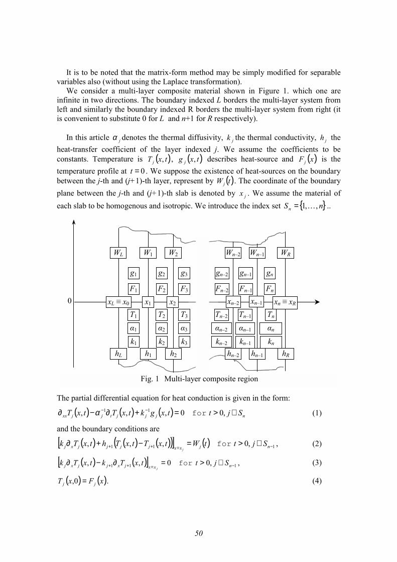
50

It is to be noted that the matrix-form method may be simply modified for separablevariables also (without using the Laplace transformation).

We consider a multi-layer composite material shown in Figure 1. which one areinfinite in two directions. The boundary indexed L borders the multi-layer system fromleft and similarly the boundary indexed R borders the multi-layer system from right (itis convenient to substitute 0 for L and n+1 for R respectively).

In this article jα denotes the thermal diffusivity, jk the thermal conductivity, jh theheat-transfer coefficient of the layer indexed j. We assume the coefficients to beconstants. Temperature is ( )txT j , , ( )txg j , describes heat-source and ( )xF j is thetemperature profile at 0=t . We suppose the existence of heat-sources on the boundarybetween the j-th and (j+1)-th layer, represent by ( )tWj . The coordinate of the boundaryplane between the j-th and (j+1)-th slab is denoted by jx . We assume the material ofeach slab to be homogenous and isotropic. We introduce the index set nSn ,,1 "= ..

The partial differential equation for heat conduction is given in the form:

( ) ( ) ( ) njjjtjjxx SjttxgktxTtxT ∈>=+∂−∂ −− ,00,,, 11 forα (1)

and the boundary conditions are

( ) ( ) ( )( )[ ] ( ) ,,0,,, 111 −=++ ∈>=−+∂ njxxjjjjxj SjttWtxTtxThtxTkj

for (2)

( ) ( )[ ] ,,00,, 111 −=++ ∈>=∂−∂ nxxjxjjxj SjttxTktxTkj

for (3)

( ) ( ).0, xFxT jj = (4)

0 xL ≡ x0 x1 x2 xn–1 xn ≡ xR

g1 g2 gn–1 gn

WL W1 W2 WRWn–1Wn–2

xn–2

g3 gn–2

F1 F2 Fn–1 FnF3 Fn–2

hL h1 h2 hRhn–1hn–2

T1 T2 Tn–1 TnT3 Tn–2

α1 α2 αn–1 αnα3 αn–2

k1 k2 kn–1 knk3 kn–2

Fig. 1 Multi-layer composite region

51

For the left and right boundaries we have

( ) ( )[ ] ( ),,, 11 tWtxThtxTk LxxLxL L=−∂ = (5)

( ) ( )[ ] ( ).,, tWtxThtxTk RxxnRnxR R=+∂ = (6)

The Laplace transform sL of these equations gives the following differentialequations

( ) ( ) ( )( ) ( ) ( ) ( ) ( ) ( ) ( ) ,,,,,,,,

0,,,1

1

txgsxsxkxFsxtxTsx

Sjsxsxssx

jjjjjjjj

njjjjxx

ss LL ≡+≡Γ≡

∈=Γ+−∂−

−

γγθ

θαθ

and

wherefor

(7)

( ) ( ) ( )( )[ ] ( )( ) ( ) ,

,,, 111

tWs

Sjssxsxhsxk

jsj

njxxjjjjxjj

L≡

∈=−+∂ −=++

ω

ωθθθ wherefor(8)

( ) ( )[ ] ,0,, 111 −=++ ∈=∂−∂ nxxjxjjxj Sjsxksxkj

forθθ (9)

( ) ( )[ ] ( ) ( ) ( ) andwhere tWsssxhsxk LsLLxxLxL LL≡=−∂ = ωωθθ ,, 11 (10)

( ) ( )[ ] ( ) ( ) ( ) .,, tWLsssxhsxk RsRRxxnRnxR R≡=+∂ = ωωθθ where (11)

We can write the general solutions of the system of differential equations (7) in theform

( ) ( ) ( ) ( ) npjjjjjj SjsxsxAsxAsx ∈++= ++−− ,,,, θθθθ (12)

where ( ) ( )sxsx jj ,, ++ θθ and are independent solutions of the homogenous equations

obtained from (7). Functions ( )sxpj ,θ are partial solutions of the inhomogeneous system

of equations in the interval (xj–1, xj). One of the forms of independent homogenoussolutions is:

( ) ( ) .cosh,sinh, nj

jj

j Sjxssxxssx ∈

=

= +−

αθ

αθ and (13)

We keep the general form of the solutions for farther calculations:

2 The matrix-form solutions

We can express the system of differential equations (8), (9), (10) and (11) using (12), asa system of linear equations for the set of 2n unknown variables

nSjjj AA∈

+− , as follows

.ZM.A = (14)

The matrix M is a band-diagonal square matrix with block elements

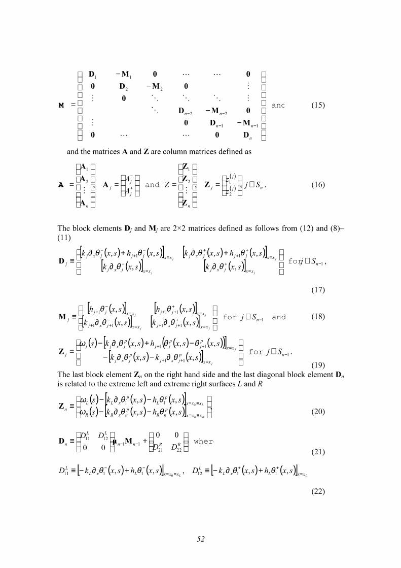
52

and

−−

−−

=

−−

−−

n

nn

nn

D00MD00MD

00MD0

00MD

!!

#

$

#$$$#

#

!!

11

22

22

11

M (15)

and the matrices A and Z are column matrices defined as

( )

( ) .,,,2

12

1

2

1

nj

j

j

n

j

jj

n

Sjzz

ZAA

∈

=

=

=

= +

−

Z

Z

ZZ

A

A

AA

##andA (16)

The block elements Dj and Mj are 2×2 matrices defined as follows from (12) and (8)–(11)

( ) ( )[ ] ( ) ( )[ ]( )[ ] ( )[ ] ,

,,

,,,,1

11

−=

+=

−=

++

+=

−+

−

∈

∂∂

+∂+∂≡ n

xxjxjxxjxj

xxjjjxjxxjjjxj

j Sjsxksxk

sxhsxksxhsxk

jj

jj forθθ

θθθθD

(17)

( )[ ] ( )[ ]( )[ ] ( )[ ] andfor 1

1111

111

,,

,,−

=+++=

−++

=+++=

−+

∈

∂∂≡ n

xxjxjxxjxj

xxjjxxjj

j Sjsxksxk

sxhsxh

jj

jj

θθ

θθM (18)

( ) ( ) ( ) ( )( )[ ]( ) ( )[ ] .

,,

,,,1

11

11

−=++

=++∈

∂−∂−

−+∂−= n

xxpjxj

pjxj

xxpj

pjj

pjxjj

j Sjsxksxk

sxsxhsxks

j

j forθθ

θθθωZ

(19)The last block element Zn on the right hand side and the last diagonal block element Dnis related to the extreme left and extreme right surfaces L and R

( ) ( ) ( )[ ]( ) ( ) ( )[ ] ,

,,,,

011

−∂−−∂−

≡≡=

≡=

Rn

L

xxxp

nRp

nxRR

xxxp

Lp

xLLn sxhsxks

sxhsxksθθωθθω

Z(20)

where

+

≡ −− RRnn

LL

n DDDD

222111

1211 0000

MμD(21)

( ) ( )[ ] ( ) ( )[ ]LL xxLxL

LxxxLxL

L sxhsxkDsxhsxkD =++

≡=−− +∂−≡+∂−≡ ,,,,, 11121111 0

θθθθ

(22)

53

( ) ( )[ ] ( ) ( )[ ]RRn xxnRnxR

RxxxnRnxR

R sxhsxkDsxhsxkD =++

≡=−− +∂≡+∂≡ ,,,,, 2221 θθθθ (23)

further

( )( ) ( ) .2, 11

112

121

11

111 njjjjj ≤≤== −

−−

−−−− forDMDMDMDμDμ " (24)

The regularity of all matrices Dj and Mj-1 follows from the independent ness of+−jandθθ j – see (17), (18).

We obtain the solution for An from (15)

.1nnn ZDA −= (25)

Further we obtain

1111

+−−− += jjjjjj AMDZDA (26)

The relation between A1 and Aj is given by

where111 , −+ ∈+= njjjj SjAMμζA (27)

nSl

lljjj Sjj

∈=+++= ∑∈

ZμZμZμZμζ "2211

(28)

3 Special matrix-form solution with two heat-sources

Consider a multi-layer system of slabs defined in this article with an additionalassumption, that the only heat source is on the extreme left or extreme right slabindexed as L and R respectively. The temperature is equal to zero everywhere in themulti-layer system at t = 0. In this case the following conditions are fulfilled

( )( )( ) .00

,00,

,,0

1−∈>≡

∈>≡

∈≡

nj

nj

nj

SjttWSjttxg

SjxF

andallfor

andallfor (29)

In this case

,0 1−∈≡ nj Sjallfor ζ (30)

therefore:

.,,2

,

111

11

11

111111

1

njnnnnjjj

nnnnnnn

nnn

"==

==

=

−−−

−−

−−

−−−−−

−

ZDMμμMAZDMμAMμA

ZDAfinal and (31)

54

4 Conclusion

We present the matrix-form method of solving heat conduction in a multi-layeredsystem that consists of n plan-parallel slabs. The great advantage of the matrix-formsolutions is evident for multi-layer systems with analogous boundary conditions andinitial conditions for all the slabs of the system.

The solution is completed if we know all the 2n coefficients −jA and +

jA . Thestarting point is given by the solution of the equation (25). We obtain all the A-coefficients using the relations (26 – 28). The solution is found in Laplace-space (see13).

The structure of the solutions reflects the structure of physical properties andconditions in the slabs. The matrices Dj, Mj and Zj represent the physical reality of theconnection between adjoining slabs. The matrix-form representation is convenient formodeling by the method of multi-pole approach of the solutions (see [3]), or any othermethods.

Acknowledgement

Authors wish to thank the Slovak Science Grant Agency for the financial support underthe contract 1/6115/99.

References

[1] Hohenauer W, Vozár L, 1999 An Estimation of Thermophysical Properties ofLayered Materials using the Laser Flash Method, High Temp. High Press, preprint

[2] Araki N, Makino A, Ishiguro A and Mihara J; 1992 An Analytical Solution of theTemperature Response in Multilayered Materials for Transient Methods; Int. J.Thermophys., 13, 515-538

[3] Carslaw H S., Jaeger J C, 1959 Conduction of Heat in Solids, (Oxford, ClarendonPress)