HAL Id: hal-01152775https://hal-mines-paristech.archives-ouvertes.fr/hal-01152775

Submitted on 12 Jan 2016

HAL is a multi-disciplinary open accessarchive for the deposit and dissemination of sci-entific research documents, whether they are pub-lished or not. The documents may come fromteaching and research institutions in France orabroad, or from public or private research centers.

L’archive ouverte pluridisciplinaire HAL, estdestinée au dépôt et à la diffusion de documentsscientifiques de niveau recherche, publiés ou non,émanant des établissements d’enseignement et derecherche français ou étrangers, des laboratoirespublics ou privés.

Thermophysical Properties, Hydrate and PhaseBehaviour Modelling in Acid Gas-Rich Systems

Antonin Chapoy, Rod Burgass, Bahman Tohidi, Martha Hajiw, ChristopheCoquelet

To cite this version:Antonin Chapoy, Rod Burgass, Bahman Tohidi, Martha Hajiw, Christophe Coquelet. Thermophys-ical Properties, Hydrate and Phase Behaviour Modelling in Acid Gas-Rich Systems . AGIS - 5thInternational Acid Gas Injection, May 2015, BANFF, Canada. �hal-01152775�

Thermophysical Properties, Hydrate and Phase Behaviour Modelling in

Acid Gas-Rich Systems

Antonin Chapoy1,2*

, Rod Burgass1, Bahman Tohidi

1

Martha Hajiw1,2

, Christophe Coquelet2

1Hydrates, Flow Assurance & Phase Equilibria Research Group, Institute of Petroleum

Engineering, Heriot-Watt University, Edinburgh EH14 4AS, Scotland, UK 2Mines ParisTech, PSL Research University CTP, Centre Thermodynamique des Procédés -

Département Énergétique et Procédés, Fontainebleau, France

Abstract In this communication we present experimental techniques, equipment and

thermodynamic modelling for investigating systems with high acid gas concentrations and

discuss experimental results on the phase behaviour and thermo-physical properties of acid

gas-rich systems. The effect of high CO2 concentration on density and viscosity were

experimentally and theoretically investigated over a wide range of temperature and pressures.

A corresponding-state model was developed to predict the viscosity of the stream and a

volume corrected equation of state approach was used to calculate densities. The phase

envelope and the hydrate stability (in water saturated and under-saturated conditions to assess

dehydration requirements) of some acid gas-rich fluids were also experimentally determined

to test a generalized model, which was developed to predict the phase behaviour, hydrate

dissociation pressures and the dehydration requirements of acid gas rich gases.

1.1 Introduction As the global demand for natural gas is forecasted to steadily grow, the demand will be met

by supplies produced from “unconventional” gases. With sour gas fields worldwide

accounting for some 40% of natural gas reserves, the development and production of these

reserves are under very serious consideration (Lallemand et al. 2012). The main challenges

facing companies developing these fields with high concentrations of acid gases are reservoir

engineering, phase behaviour predictions, processing and their removal from hydrocarbon

streams, transportation and storage.

Due to the huge quantities of these gases produced and more stringent environmental

regulations these gases cannot be flared, thus one of the most viable options is to inject them

back into the reservoir for storage as well as enhance oil recovery (EOR). For acid gases, the

disposal alternatives are: injection of compressed acid gas into the formation; disposal of acid

gases with the formation water or solubilise acid gases into a light hydrocarbon solvent and

use the solvent as a miscible flood EOR (Jamaluddin et al., 1996). In fields with high

concentration of H2S dehydration using glycols may lead to additional problems such as

corrosion and the release of H2S when it is regenerated. In such cases the knowledge of

* To whom correspondence should be addressed: e-mail: antonin.chapoy@pet.hw.ac.uk

multicomponent gas water content and the optimum injection pressure will be essential.

Furthermore reinjection into new reservoirs (such as Kashagan field in Kazakhstan) will

require extremely high pressures. The design of such compressors requires accurate thermo-

physical properties of multicomponent mixtures.

However limited data are available on the phase and hydrate behaviours of CO2-rich or

acid gas systems to validate existing thermodynamic models. Therefore the applicability of

the existing models and their uncertainties can lead to over or undersized designs. In this

communication we present experimental techniques, equipment and thermodynamic

modelling for investigating systems with high CO2 or H2S concentrations, including gas

reservoirs with high CO2 content and/or CO2-rich systems from capture processes. In

particular, experimental measurements of the locus of incipient hydrate-liquid water-vapour

curve for a methane – H2S binary system and a CO2-rich natural gas (70 mole % of CO2 and

30 mole % of light hydrocarbons C1 to nC4) in equilibrium with liquid water are presented at

pressures up to 35 MPa. Experimental data are reported for water content in equilibrium with

hydrates at about 150 bar and temperature range from 233 to 283 K. Density and viscosity of

the mixture were also measured from 253 to 423 K at pressure up to 124 MPa. An example of

dry ice formation in a CO2-rich natural gas will be also described.

The Cubic-Plus-Association (CPA-EoS) or the Soave-Redlich-Kwong (SRK) equation

of state combined with the solid solution theory of van der Waals and Platteeuw (1959) as

developed by Parrish and Prausnitz (1972) was employed to model the fluid and hydrate

phase equilibria as previously described by Chapoy et al. (2012). The predictions of the

thermodynamic model were compared with the experimentally measured properties

(saturation pressure, dew point, frost points, hydrates). A corresponding state model

developed to predict viscosity of the CO2-rich stream (Chapoy et al. 2013) was used to

evaluate the new viscosity data.

1.2 Experimental Setups and Procedures

The majority of the setups and procedures used in this paper were described in detail in

Chapoy et al. (2005), Chapoy et al. (2012), Chapoy et al. (2013) and Hajiw et al. (2014). A

brief description of each setup is given below.

1.2.1 Saturation and Dew Pressure Measurements and Procedures

The equilibrium setup consisted of a piston-type variable volume (maximum effective

volume of 300 ml), titanium cylindrical pressure vessel with mixing ball, mounted on a

horizontal pivot with associated stand for pneumatic controlled rocking mechanism. Rocking

of the cell through 180 degrees at a constant rate, and the subsequent movement of the

mixing ball within it, ensured adequate mixing of the cell fluids. Cell volume, hence pressure,

can be adjusted by injecting/withdrawal of liquid behind the moving piston. The rig has a

working temperature range of 210 to 370 K, with a maximum operating pressure of 69 MPa.

System temperature is controlled by circulating coolant from a cryostat within a jacket

surrounding the cell. The equilibrium cell and pipework were thoroughly insulated to ensure

constant temperature. The temperature was measured and monitored by means of a PRT

(Platinum Resistance Thermometers) located within the cooling jacket of the cell (accuracy

of ±0.05 K). A Quartzdyne pressure transducer with an accuracy of ± 0.05 MPa was used to

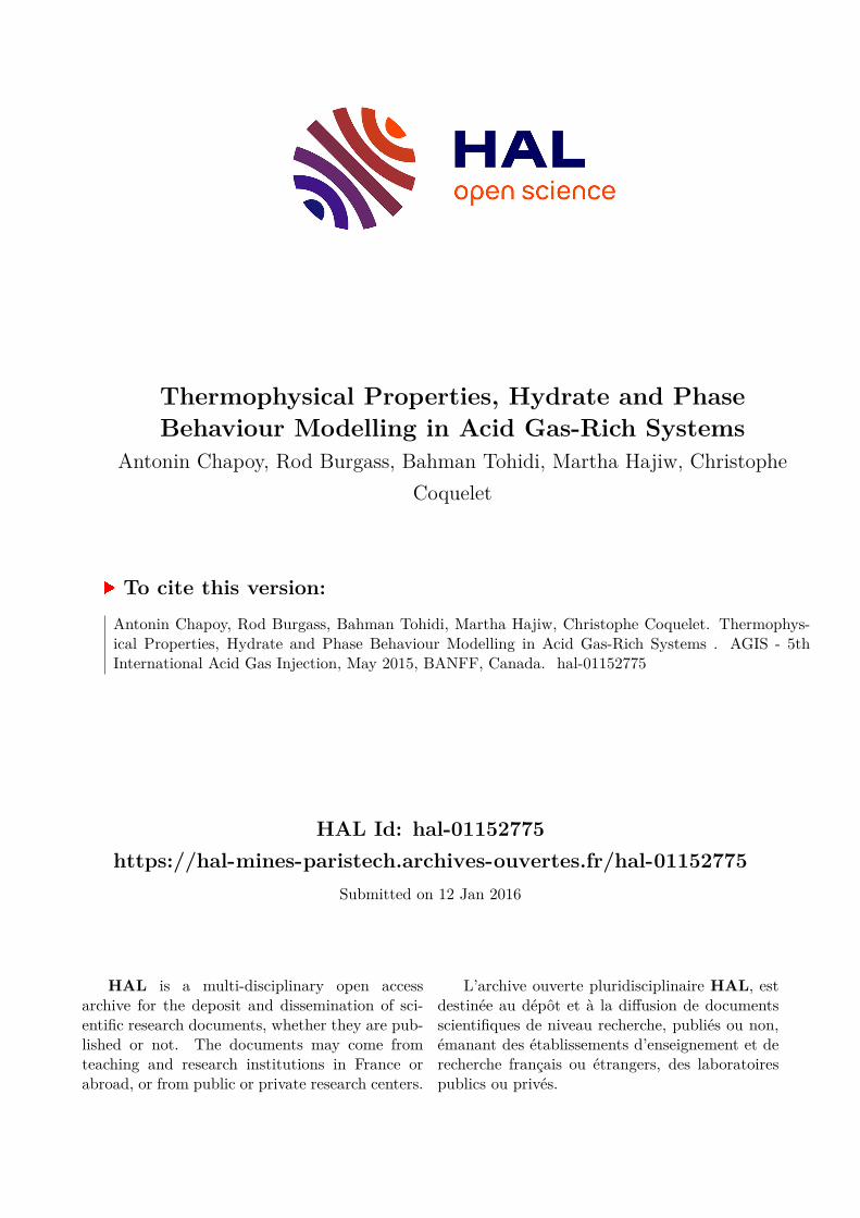
monitor pressure. The bubble point was determined by changing the volume of the cell and

finding the break over point in the pressure vs. volume curve as shown in Figure 1.

A typical test to determine the dew point is as follows: To obtain the dew point using

the isochoric method the cell is loaded with the test sample and is set to 5 degrees above the

estimated dew point temperature. The cell is cooled until the system has clearly become two

phase. The cell temperature is then step heated, allowing sufficient time for equilibration,

until the system has clearly become single phase again. Throughout the process the cell is

rocked using a pneumatic pivoting system to ensure all of the cell constituents are thoroughly

mixed and equilibrium is reached. The system pressure and temperature are recorded every

minute using a logging program. The recorded data is then processed to determine the system

pressure at each temperature step. This process results in two traces with very different slopes

on a pressure versus temperature (P/T) plot, one in the single phase and one in the 2 phases

region. The point where these two traces intersect is taken as the dew point (Figure 2).

Pre

ssu

re

Volume / cm3

2 Phases Region

Single Phase Region

Figure 1. Plot showing an example of bubble point determination from plot of change in cell

pressure versus volume

Pre

ssu

re

Temperature

Cooling

Heating

Dew Point

Single Phase Region

2 Phases Region

Figure 2. Plot showing an example of dew point determinations from equilibrium step-

heating data using the isochoric method.

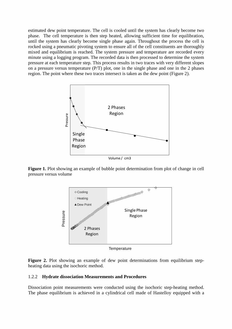
1.2.2 Hydrate dissociation Measurements and Procedures

Dissociation point measurements were conducted using the isochoric step-heating method.

The phase equilibrium is achieved in a cylindrical cell made of Hastelloy equipped with a

pressure magnetic mixer. A detailed description of the apparatus and test procedure can be

found elsewhere (Hajiw et al., 2014; Chapoy et al., 2013). The weight of the fluids (i.e.,

water and the multicomponent fluid) injected are recorded prior to any measurements and the

overall feed composition can thus be calculated.

A typical test to determine the dissociation point is as follows: the cell is cleaned and dried.

About half of the volume of the cell is initially preloaded with water, prior to applying

vacuum to the system. Then, the fluids are loaded into the cell to reach the first desired

pressure the temperature is then increased stepwise, slowly enough to allow equilibrium to be

achieved at each temperature step. At temperatures below the point of complete dissociation,

gas is released from decomposing hydrates, giving a marked rise in the cell pressure with

each temperature step (Figure 3). However, once the cell temperature has passed the final

hydrate dissociation point, and all hydrates have disappeared from the system, a further rise

in the temperature will result only in a relatively small pressure rise due to thermal expansion.

This process results in two traces with very different slopes on a pressure versus temperature

(P/T) plot; one before and one after the dissociation point. The point where these two traces

intersect (i.e., an abrupt change in the slope of the P/T plot) is taken was the dissociation

point (see Figure 3).

For a full discussion on accuracy and uncertainties of hydrate dissociations measurements the

reader is invited to check the work of Stringari et al. (2014) or Hajiw, (2014).

T

P

Hydrate dissociation + Thermal expansion

Thermal expansion

Dissociation Point

No hydrate

Hydrate dissociation

and gas release

Figure 3. Dissociation point determination from equilibrium step-heating data. The

equilibrium dissociation point is determined as being the intersection between the hydrate

dissociation (pressure increase as a result of gas release due to temperature increase and

hydrate dissociation, as well as thermal expansion) and the linear thermal expansion (no

hydrate) curves.

1.2.3 Water Content Measurements and Procedures

The core of the equipment for water content measurement has been originally described by

Chapoy et al. (2012) and Burgass et al. (2014). The setup comprises of an equilibrium cell

and a device for measuring the water content of equilibrated fluids passed from the cell. The

equilibrium cell is similar to the one described in the saturation pressure measurements. The

moisture/water content measurement set-up consists of a heated line, a Tuneable Diode Laser

Adsorption Spectroscopy (TDLAS) from Yokogawa and a flow meter. The estimated

experimental accuracy of water content is ±5 ppm mole.

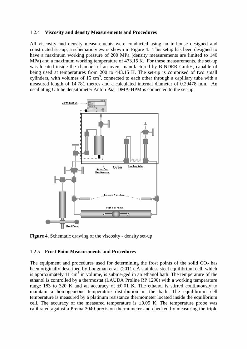
1.2.4 Viscosity and density Measurements and Procedures

All viscosity and density measurements were conducted using an in-house designed and

constructed set-up; a schematic view is shown in Figure 4. This setup has been designed to

have a maximum working pressure of 200 MPa (density measurements are limited to 140

MPa) and a maximum working temperature of 473.15 K. For these measurements, the set-up

was located inside the chamber of an oven, manufactured by BINDER GmbH, capable of

being used at temperatures from 200 to 443.15 K. The set-up is comprised of two small

cylinders, with volumes of 15 cm3, connected to each other through a capillary tube with a

measured length of 14.781 metres and a calculated internal diameter of 0.29478 mm. An

oscillating U tube densitometer Anton Paar DMA-HPM is connected to the set-up.

Figure 4. Schematic drawing of the viscosity - density set-up

1.2.5 Frost Point Measurements and Procedures

The equipment and procedures used for determining the frost points of the solid CO2 has

been originally described by Longman et al. (2011). A stainless steel equilibrium cell, which

is approximately 11 cm3 in volume, is submerged in an ethanol bath. The temperature of the

ethanol is controlled by a thermostat (LAUDA Proline RP 1290) with a working temperature

range 183 to 320 K and an accuracy of ±0.01 K. The ethanol is stirred continuously to

maintain a homogeneous temperature distribution in the bath. The equilibrium cell

temperature is measured by a platinum resistance thermometer located inside the equilibrium

cell. The accuracy of the measured temperature is ±0.05 K. The temperature probe was

calibrated against a Prema 3040 precision thermometer and checked by measuring the triple

point of pure CO2. The equilibrium cell pressure is measured by a Quartzdyne pressure

transducer.

1.2.6 Materials

Methane and hydrogen sulphide were purchased from Air Liquide with 99.995 vol%

certified purity for methane and 99.5 vol% for hydrogen sulphide. Deionised water was used

in all experiments. Carbon dioxide (CO2) has been purchased from BOC with a certified

purity higher than 99.995 vol%. Compositions of the synthetic mixtures are given in Table 3.

Table 1. Composition, mole% each component, of the multicomponent mixtures

Components Synthetic Mix 1

(from Hajiw et al., 2014)

Synthetic Mix 2

(from Chapoy et al., 2013) Synthetic Mix 3

CO2 - Balance (89.83) Balance (69.99)

H2S 20.0 - -

Methane 80.0 - 20.02 (±0.11%)

Ethane - - 6.612 (±0.034%)

Propane - - 2.58 (±0.013%)

i-Butane - - 0.3998 (±0.004%)

n-Butane - - 0.3997(±0.004%)

Nitrogen - 3.07(±0.04%) -

Oxygen - 5.05(±0.01%) -

Argon - 2.05(±0.06%) -

Total 100 100 100

1.3 Thermodynamic and Viscosity Modelling

1.3.1 Fluid and Hydrate Phase Equilibria Model

A detailed description of the original thermodynamic framework used in this work

can be found elsewhere (Haghighi et al., 2009; Chapoy et al., 2014). In summary, the

thermodynamic model is based on the uniformity of fugacity of each component throughout

all the phases. The CPA-EoS or the SRK-EoS (if no water is present) is used to determine

the component fugacities in fluid phases. The hydrate phase is modelled using the solid

solution theory of van der Waals and Platteeuw (1954) as developed by Parrish and Prausnitz

(1972). The CPA-EoS binary interaction parameters between components were determined

using the group contribution method developed by Jaubert and co-workers. The model to

calculate frost points was described by Longman et al. (2011). The developed model can

predict accurately the distribution of water in the CO2 or H2S-rich phase and solubility of

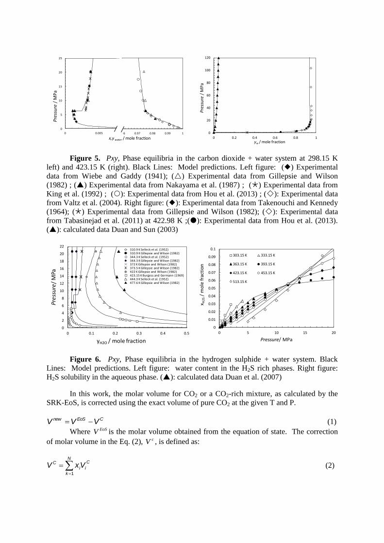
CO2 or H2S in the aqueous phase below and above the critical point of pure CO2 as shown in

Figures 5 and 6.

0

5

10

15

20

25

0 0.005

Pre

ssu

re/

MP

a

x,y water / mole fraction0.96 0.97 0.98 0.99 1

0

20

40

60

80

100

120

0 0.2 0.4 0.6 0.8 1

Pre

ssu

re/

MP

a

yw / mole fraction

Figure 5. Pxy, Phase equilibria in the carbon dioxide + water system at 298.15 K

left) and 423.15 K (right). Black Lines: Model predictions. Left figure: () Experimental

data from Wiebe and Gaddy (1941); () Experimental data from Gillepsie and Wilson

(1982) ; () Experimental data from Nakayama et al. (1987) ; () Experimental data from

King et al. (1992) ; (): Experimental data from Hou et al. (2013) ; (): Experimental data

from Valtz et al. (2004). Right figure: (): Experimental data from Takenouchi and Kennedy

(1964); () Experimental data from Gillepsie and Wilson (1982); (): Experimental data

from Tabasinejad et al. (2011) at 422.98 K ;(): Experimental data from Hou et al. (2013).

(): calculated data Duan and Sun (2003)

0

2

4

6

8

10

12

14

16

18

20

22

0 0.1 0.2 0.3 0.4 0.5

Pre

ssu

re/

MPa

yH2O / mole fraction

310.9 K Selleck et al. (1952)310.9 K Gillepsie and Wilson (1982)344.3 K Selleck et al. (1952)344.3 K Gillepsie and Wilson (1982)372 K Gillepsie and Wilson (1982)373.5 K Gillepsie and Wilson (1982)422 K Gillepsie and Wilson (1982)423.15 K Burgess and Germann (1969)444.3 K Selleck et al. (1952)477.6 K Gillepsie and Wilson (1982)

0

0.01

0.02

0.03

0.04

0.05

0.06

0.07

0.08

0.09

0.1

0 5 10 15 20

x H2S

/ m

ole

fra

ctio

n

Pressure/ MPa

303.15 K 333.15 K

363.15 K 393.15 K

423.15 K 453.15 K

513.15 K

Figure 6. Pxy, Phase equilibria in the hydrogen sulphide + water system. Black

Lines: Model predictions. Left figure: water content in the H2S rich phases. Right figure:

H2S solubility in the aqueous phase. (): calculated data Duan et al. (2007)

In this work, the molar volume for CO2 or a CO2-rich mixture, as calculated by the

SRK-EoS, is corrected using the exact volume of pure CO2 at the given T and P.

CEoSnew VVV (1)

Where EoSV is the molar volume obtained from the equation of state. The correction

of molar volume in the Eq. (2), cV , is defined as:

C

i

N

k

i

C VxV

1

(2)

xi is the composition of component i in the phase in which the volume is calculated. For CO2, c

iV is defined by

MBWREoS

COPure

C

CO VVV 22

(3)

For the other components, c

iV was set to 0. The carbon dioxide density is computed from the

MBWR equation in the form suggested by Ely et al. (1987):

29 15

2 17

1 10

( ) ( )n n

n n

n n

P a T a T e

(4)

1.3.2 Viscosity Model

To model viscosity, our proposed model is a modification of the corresponding state viscosity

model described in Pedersen and Christensen (2007). According to the corresponding states

principles applied to viscosity, the reduced viscosity, C

r

PT

),( , for two components at

the same reduced pressure,C

r PPP and reduced temperature,

Cr T

TT ,will be the same.

),( rrr PTf (5)

Based on the dilute gases considerations and kinetic theory, viscosity at critical point can be

approximated as:

6/1

2/13/2

c

cc

T

MP (6)

Where, M denotes the Molecular weight. Thus, the reduced viscosity can be expressed as:

2/13/2

6/1),(),(

MP

TPTPT

c

c

C

r

(7)

For one component as a reference component if the function f in Eq. (5) is known, it is

possible to calculate the viscosity of any other components, such as component i, at any

pressure and temperature. Thus,

ic

co

ic

co

oc

ic

o

i

oc

ic

iP

PP

T

TT

T

T

M

M

P

P

,,

06

1

,

,

21

32

,

,

, (8)

Where, 0 refers to the reference component. Methane with the viscosity data published by

Hanley et al. (1975) was selected as the reference fluid in the original Pedersen model. In

this work, CO2 with the viscosity data published by Fenghour et al. (1998) has been selected

as the reference fluid as CO2 is the major constituent of the stream. The viscosity of CO2 as a

function of density at given T and P can be calculated from the following equation:

),()(),( 0 TTT (9)

Where, η0(T) is the zero-density viscosity which can be obtained from the following

equation:

)(

00697.1 2/1

0

T

TT

(10)

In this equation, the zero-density viscosity is in units of Pa.s and temperature, T, in K. The

reduced effective cross section, )( T , is represented by the empirical equation:

4

0

)(lnlni

i

i TaT (11)

Where the reduced temperature, T*, is given by:

T*=kT/ε (12)

And the energy scaling parameter, ε/k =251.196 K. The coefficients ai are listed in Table 1.

The second contribution in Eq. (9) is the excess viscosity, ),( T , which describes how the

viscosity can change as a function of density outside of the critical region. The excess

viscosity term can be correlated as follows:

*

8

828

813*

6

642

2111,T

dd

T

dddT

(13)

Where, the temperature is in Kelvin, the density in kg/m3 and the excess viscosity in Pa.s.

The coefficients dij are shown in Table 2.

Table 1. Values of Coefficients ai for CO2 in

Eq. (11)

Table 2. Values of coefficients dij in Eq. (13)

i ai

0 0.235156

1 -0.491266

2 5.211155 x 10-2

3 5.347906 x 10-2

4 -1.537102 x 10-2

dij Value

d11 0.4071119 x 10-2

d21 0.7198037 x 10-4

d64 0.2411697 x 10-16

d81 0.2971072 x 10-22

d82 -0.1627888 x 10-22

The corresponding states principle expressed in Eq. (8) for the viscosity of pure components

works well for mixtures. Pedersen et al. (1984) have used the following expression to

calculate the viscosity of mixtures at any pressure and temperature.

0006

1

,

,

21

32

,

,

,PT

T

T

M

M

P

P

o

mix

oc

mixc

o

mix

oc

mixc

mix

(14)

Where

mixmixc

coo

P

PPP

0

,

and mixmixc

coo

T

TTT

0

,

(15)

The critical temperature and pressure for mixtures, according to recommended mixing rules

by Murad and Gubbins (1977), can be found from:

N

i

N

j jc

jc

ic

icji

N

ijcic

N

j jc

jc

ic

icji

mixc

P

T

P

Tzz

TTP

T

P

Tzz

T33/1

,

,

3/1

,

,

,,

33/1

,

,

3/1

,

,

, (16)

233/1

,

,

3/1

,

,

,,

33/1

,

,

3/1

,

,

,

8

N

i

N

j jc

jc

ic

icji

N

ijcic

N

j jc

jc

ic

icji

mixc

P

T

P

Tzz

TTP

T

P

Tzz

P (17)

The mixture molecular weight is found from

nnwmix MMMM 303.2303.2410304.1 (18)

Where wM and nM are the weight average and number average molecular weights,

respectively.

N

iii

N

iii

w

Mz

Mz

M

2

(19)

N

i

iin MzM (20)

The parameter for mixtures in Eq. (14) can be found from: 5173.0847.1310378.7000.1 mixrmix M (21)

Also, for the reference fluid can be found from Eq. (21) by replacing the molecular weight

of the mixture with that of the reference fluid, carbon dioxide. The reduced density, ρr, is

defined as:

0

,,

0 ,

c

mixc

co

mixc

co

r

P

PP

T

TT

(22)

The critical density of carbon dioxide, ρ0, is equal to 467.69 kg/m3. The Modified Benedict–

Webb–Rubin (MBWR) equation of state has been applied for computing the reference fluid

density, ρ0, at the desired pressure and temperature of mixc

co

P

PP

,

, mixc

co

T

TT

,

.

The procedure below should be followed to calculate the viscosity of CO2 systems with

impurities by the proposed corresponding state principle model:

1. Calculate the Tcmix, Pcmix and Mmix from Eq. (16), (17) and (18), respectively.

2. Obtain the CO2 density at mixc

co

P

PP

,

, mixc

co

T

TT

,

from the MBWR EOS and calculate the

reduced density from Equation (22).

3. The mixture parameter, mix, and 0 should be calculated from Eq. (21).

4. The reference pressure and temperature, P0 and T0, should be calculated from

Equation (15).

5. Calculate the CO2 reference fluid, ),( 000 TP in Eq. (14) from Eq. (9).

6. Calculate the mixture viscosity from Eq. (14).

1.4 Results and Discussions

All results were compared where possible with experimental values for pure methane, pure

carbon dioxide, a synthetic CO2-rich fluid (CO2: 89.83 mole%; O2: 5.05 mole%; Ar: 2.05

mole%; N2: 3.07 mole% from Chapoy et al., 2013) and a typical North Sea natural gas.

For a model to predict accurately the hydrate phase behaviour or transport properties,

it is essential that the phase behaviour is correctly predicted, i.e. the phase region, bubble and

dew lines. For example for hydrate calculation, the hydrate stability has very sharp

temperature dependency above the bubble point, an error in estimating the saturation pressure

will lead to high deviations in the hydrate phase behaviour. Viscosity models are also

dependant on good density predictions, if a vapour-liquid behaviour is predicted instead of a

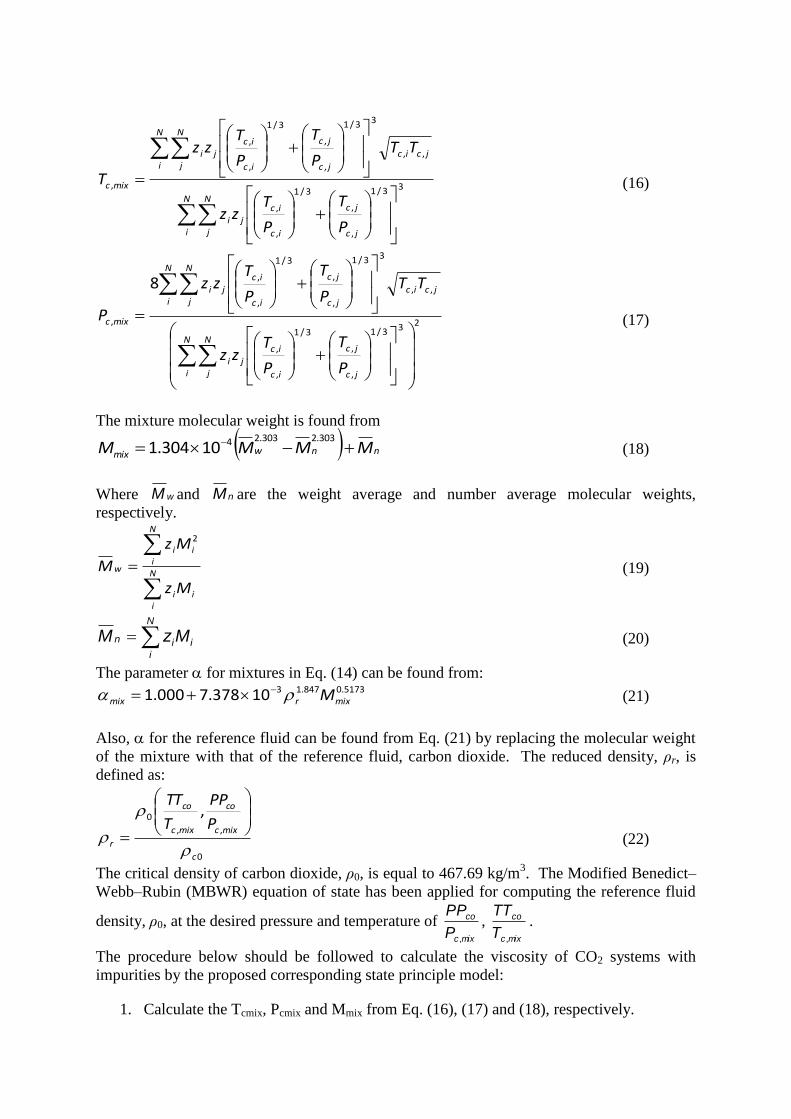
saturated liquid it will also lead to very high deviations in viscosities. As shown in Figure 7,

the SRK-EoS model combined with the group contribution for kij can predict the phase

envelope of the multicomponent systems with good accuracy. The predictions are of greater

accuracy for the system containing less carbon dioxide.

0

1

2

3

4

5

6

7

8

9

10

223.15 243.15 263.15 283.15 303.15

Pre

ssu

re/M

Pa

Temperature / K

Figure 7. Experimental and predicted phase envelope of the CO2-rich mixture. (),Synthetic

Mix 3. (), Synthetic Mix 2. Black lines: bubble lines predictions using the SRK-EoS;

Dotted black lines: dew lines predictions using the SRK-EoS; Grey broken lines: predicted

vapour pressure of pure CO2 using the SRK-EoS.

0

5

10

15

20

25

30

35

40

273.15 283.15 293.15 303.15 313.15

Pre

ssu

re/M

Pa

Temperature / K

Figure 8. Experimental and predicted hydrate stability of CO2, H2S and methane in

equilibrium with liquid water. (), pure CO2 hydrate stability zone (Chapoy et al. 2011);

(), pure H2S hydrate stability zone (Selleck et al. 1952); (): pure CH4 hydrate stability

zone (Nixdorf and Oellrich, 1997) ;(), pure CH4 hydrate stability zone (Marshall et al.

1964).

Methane, carbon dioxide and hydrogen sulphide are well known structure I hydrate

formers. Hydrate phase equilibria of these systems have been extensively investigated and

can be predicted with very high accuracy as seen in Figure 8. Multicomponent systems

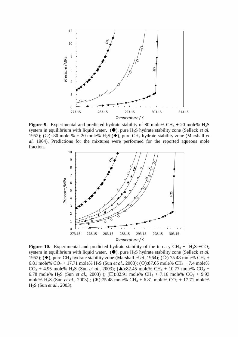
containing hydrogen sulphide are far scarcer. Hajiw et al. (2014) measured the hydrate

dissociation conditions for a mixture of methane and hydrogen sulphide. Composition of the

fluid is given in Table 1. As the solubility difference between methane and hydrogen

sulphide is of several order of magnitude, the hydrate stability zone of this mixture is highly

dependent on the fluid to water ratio as seen in Figure 9. The model has also been evaluated

with the methane + hydrogen sulphide + carbon dioxide hydrate data reported by Sun et al.

(2003). Like methane, carbon dioxide and hydrogen sulphide, and all their mixtures are

predicted to form structure I hydrate. For these systems, the thermodynamic model is in

excellent agreement with these experimental data (within 0.5 K). The ratio between the water

mole fraction and the mixture fraction can have a large effect if the concentration of H2S and

CO2 is in excess of 10 mole%.

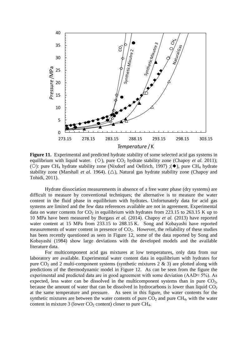
The experimental hydrate dissociation conditions for the synthetic mixtures 2 and 3 in

equilibrium with water are plotted in Figure 11. Pure CO2, CH4 and synthetic mixture 2 form

structure I hydrate whereas synthetic mixture 3 is predicted to form structure II because of the

presence of larger hydrocarbon molecules (propane, i-butane and n-butane). It is also

interesting to note that this system, depending on the water to gas ratio, should just enter the

phase envelope of the system but displays at higher pressure a liquid like hydrate locus. The

system is, over the full pressure range, more stable than pure CO2 or synthetic mixture, which

form structure I. At low and intermediate pressure (P<14 MPa), the system is also more

stable than pure CH4 hydrate, however at higher pressures where hydrates are in equilibrium

with a denser supercritical fluid, pure CH4 hydrates are more stable.

0

2

4

6

8

10

12

273.15 283.15 293.15 303.15 313.15

Pre

ssu

re/M

Pa

Temperature / K

H2S

Figure 9. Experimental and predicted hydrate stability of 80 mole% CH4 + 20 mole% H2S

system in equilibrium with liquid water. (), pure H2S hydrate stability zone (Selleck et al.

1952); (): 80 mole % + 20 mole% H2S;(), pure CH4 hydrate stability zone (Marshall et

al. 1964). Predictions for the mixtures were performed for the reported aqueous mole

fraction.

0

1

2

3

4

5

6

7

8

9

10

273.15 278.15 283.15 288.15 293.15 298.15 303.15

Pre

ssu

re/M

Pa

Temperature / K

H2S

Figure 10. Experimental and predicted hydrate stability of the ternary CH4 + H2S +CO2

system in equilibrium with liquid water. (), pure H2S hydrate stability zone (Selleck et al.

1952); (), pure CH4 hydrate stability zone (Marshall et al. 1964); () 75.48 mole% CH4 +

6.81 mole% CO2 + 17.71 mole% H2S (Sun et al., 2003); ():87.65 mole% CH4 + 7.4 mole%

CO2 + 4.95 mole% H2S (Sun et al., 2003); ():82.45 mole% CH4 + 10.77 mole% CO2 +

6.78 mole% H2S (Sun et al., 2003) ); ():82.91 mole% CH4 + 7.16 mole% CO2 + 9.93

mole% H2S (Sun et al., 2003) ; ():75.48 mole% CH4 + 6.81 mole% CO2 + 17.71 mole%

H2S (Sun et al., 2003).

0

5

10

15

20

25

30

35

40

273.15 278.15 283.15 288.15 293.15 298.15 303.15

Pre

ssu

re/M

Pa

Temperature / K

Figure 11. Experimental and predicted hydrate stability of some selected acid gas systems in

equilibrium with liquid water. (), pure CO2 hydrate stability zone (Chapoy et al. 2011);

(): pure CH4 hydrate stability zone (Nixdorf and Oellrich, 1997) ;(), pure CH4 hydrate

stability zone (Marshall et al. 1964). (), Natural gas hydrate stability zone (Chapoy and

Tohidi, 2011).

Hydrate dissociation measurements in absence of a free water phase (dry systems) are

difficult to measure by conventional techniques; the alternative is to measure the water

content in the fluid phase in equilibrium with hydrates. Unfortunately data for acid gas

systems are limited and the few data references available are not in agreement. Experimental

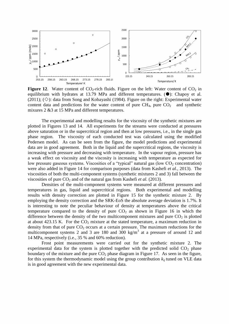
data on water contents for CO2 in equilibrium with hydrates from 223.15 to 263.15 K up to

10 MPa have been measured by Burgass et al. (2014). Chapoy et al. (2013) have reported

water content at 15 MPa from 233.15 to 288.15 K. Song and Kobayashi have reported

measurements of water content in presence of CO2. However, the reliability of these studies

has been recently questioned as seen in Figure 12, some of the data reported by Song and

Kobayashi (1984) show large deviations with the developed models and the available

literature data.

For multicomponent acid gas mixtures at low temperatures, only data from our

laboratory are available. Experimental water content data in equilibrium with hydrates for

pure CO2 and 2 multi-component systems (synthetic mixtures 2 & 3) are plotted along with

predictions of the thermodynamic model in Figure 12. As can be seen from the figure the

experimental and predicted data are in good agreement with some deviation (AAD≈ 5%). As

expected, less water can be dissolved in the multicomponent systems than in pure CO2,

because the amount of water that can be dissolved in hydrocarbons is lower than liquid CO2

at the same temperature and pressure. As seen in this figure, the water contents for the

synthetic mixtures are between the water contents of pure CO2 and pure CH4, with the water

content in mixture 3 (lower CO2 content) closer to pure CH4.

0

500

1000

1500

2000

2500

3000

253.15 258.15 263.15 268.15 273.15 278.15 283.15

yw

/ ppm

(m

ole

)

Temperature/ K

0

500

1000

1500

2000

2500

223.15 243.15 263.15 283.15

yw

/ p

pm

Temperature/ K

Figure 12. Water content of CO2-rich fluids. Figure on the left: Water content of CO2 in

equilibrium with hydrates at 13.79 MPa and different temperatures. (): Chapoy et al.

(2011); (): data from Song and Kobayashi (1984). Figure on the right: Experimental water

content data and predictions for the water content of pure CH4, pure CO2 and synthetic

mixures 2 &3 at 15 MPa and different temperatures.

The experimental and modelling results for the viscosity of the synthetic mixtures are

plotted in Figures 13 and 14. All experiments for the streams were conducted at pressures

above saturation or in the supercritical region and then at low pressures, i.e., in the single gas

phase region. The viscosity of each conducted test was calculated using the modified

Pedersen model. As can be seen from the figure, the model predictions and experimental

data are in good agreement. Both in the liquid and the supercritical regions, the viscosity is

increasing with pressure and decreasing with temperature. In the vapour region, pressure has

a weak effect on viscosity and the viscosity is increasing with temperature as expected for

low pressure gaseous systems. Viscosities of a “typical” natural gas (low CO2 concentration)

were also added in Figure 14 for comparison purposes (data from Kashefi et al., 2013). The

viscosities of both the multi-component systems (synthetic mixtures 2 and 3) fall between the

viscosities of pure CO2 and of the natural gas from Kashefi et al. (2013).

Densities of the multi-component systems were measured at different pressures and

temperatures in gas, liquid and supercritical regions. Both experimental and modelling

results with density correction are plotted in Figure 15 for the synthetic mixture 2. By

employing the density correction and the SRK-EoS the absolute average deviation is 1.7%. It

is interesting to note the peculiar behaviour of density at temperatures above the critical

temperature compared to the density of pure CO2 as shown in Figure 16 in which the

difference between the density of the two multicomponent mixtures and pure CO2 is plotted

at about 423.15 K. For the CO2 mixture at the stated temperature, a maximum reduction in

density from that of pure CO2 occurs at a certain pressure. The maximum reductions for the

multicomponent systems 2 and 3 are 180 and 300 kg/m3 at a pressure of around 12 and

14 MPa, respectively (i.e., 35 % and 60% reduction).

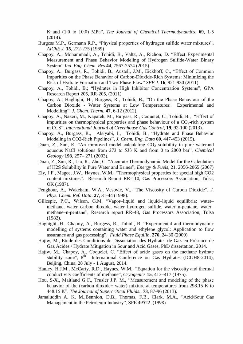
Frost point measurements were carried out for the synthetic mixture 2. The

experimental data for the system is plotted together with the predicted solid CO2 phase

boundary of the mixture and the pure CO2 phase diagram in Figure 17. As seen in the figure,

for this system the thermodynamic model using the group contribution kij tuned on VLE data

is in good agreement with the new experimental data.

0

50

100

150

200

250

300

350

0 25 50 75 100 125 150

Vis

cosi

ty, η

/

Pa.

s

P / MPa

0

20

40

60

80

100

120

140

160

180

200

0 10 20 30 40 50 60 70 80 90 100 110 120

Vis

cosi

ty, η

/

Pa.

s

Pressure / MPa Figure 13. Predicted and experimental

viscosity of synthetic mixture 2. Black

lines: Predictions using CSP model. Black

Dotted lines: Predictions using CSP model

at the bubble and dew pressures of the

system. Data inside the grey box are plotted

in Fig. 9. This work: (), T = 243.15 K

(), T = 253.15 K (), T = 273.15 K (),

T = 283.15 K (), T = 298.15 K (), T =

323.15 K (), T = 373.15 K (), T =

423.15 K

Figure 14. Predicted and experimental

viscosity of synthetic mixtures 2 and 3 at

323.15 K. Black and dotted lines: Predictions

using the modified CSP model. Grey lines:

pure CO2 viscosity. Grey broken lines:

Predictions using the original CSP model.

(), synthetic mixture 2; (),synthetic

mixture 3; () data from Kashefi et al. (2013)

for a Natural gas (in mole% C1: 88.83; C2:

5.18; C3:1.64; iC4: 0.16; nC4: 0.27; iC5: 0.04;

CO2: 2.24; N2: 1.6)

0

250

500

750

1000

1250

0 25 50 75 100 125 150

Den

sity

, ρ/

kg.

m-3

Pressure / MPa

-350

-300

-250

-200

-150

-100

-50

0

0 25 50 75 100 125 150

ρ

/ k

g.m

-3

Pressure / MPa Figure 15. Predicted and experimental

density of synthetic mixture 2. Black lines:

Predictions using the corrected SRK-EoS

model. Black Dotted lines: Predictions

using the corrected SRK-EoS model at the

bubble and dew pressures of the

system.(), T = 273.26 K (), T = 283.31

K (), T = 298.39 K (), T = 323.48 K

(), T = 373.54 K (), T = 423.43 K.

Figure 16. Predicted and experimental

density difference ρ= ρMIX

–ρCO2

, between

synthetic mixture 2 (),synthetic mixture 3

()and pure CO2 density at 323.15 K. Lines:

Predictions using the corrected SRK-EoS

model (Grey line is for methane).

0

1

2

3

4

5

6

7

8

9

10

200 220 240 260 280 300

Pre

ssu

re/M

Pa

Temperature / K

CO

2

Figure 17. Experimental and predicted phase envelope of the synthetic mixture 2. (), bubble/dew

points. (), Frost points. Black lines: bubble lines predictions using the SRK-EoS; Dotted black

lines: dew lines predictions using the SRK-EoS; Grey broken lines: phase diagram of pure CO2.

1.5 Conclusions

Knowledge on the phase behaviour and thermophysical properties of CO2-rich and acid gas

systems is of great importance for CCS and developing sour gas reservoirs, as well as testing

predictive models. However, limited published data sets are available for such systems. In

this communication the phase behaviour and some properties of different acid gas streams

have been studied, such as the phase envelope, the hydrate stability, dehydration requirement,

viscosity and density of the mixture. Models have been developed to calculate and predict

these properties.

Future work will concentrate on the determination/measurement and modelling of properties

for other types of natural gases (different CO2 concentrations, impact of H2S, etc.).

Acknowledgements This research work was part of a Joint Industrial Project (JIP) conducted jointly at the

Institute of Petroleum Engineering, Heriot-Watt University and the CTP laboratory of

MINES ParisTech. The JIPs supported by Chevron, GALP Energia, Linde AG, OMV,

Petroleum Experts, Statoil, TOTAL and National Grid Carbon Ltd, which is gratefully

acknowledged. The participation of National Grid Carbon in the JIP was funded by the

European Commission’s European Energy Programme for Recovery. The authors would also

like to thank the members of the steering committee for their fruitful comments and

discussions.

References Burgass, R., Chapoy, A., Duchet-Suchaux, P., Tohidi, B. “Experimental water content

measurements of carbon dioxide in equilibrium with hydrates at (223.15 to 263.15)

K and (1.0 to 10.0) MPa”, The Journal of Chemical Thermodynamics, 69, 1-5

(2014).

Burgess M.P., Germann R.P., “Physical properties of hydrogen sulfide water mixtures”,

AIChE J. 15, 272-275 (1969)

Chapoy, A., Mohammadi, A., Tohidi, B., Valtz, A., Richon, D. “Effect Experimental

Measurement and Phase Behavior Modeling of Hydrogen Sulfide-Water Binary

System” Ind. Eng. Chem. Res.44, 7567-7574 (2015).

Chapoy, A., Burgass, R., Tohidi, B., Austell, J.M., Eickhoff, C., “Effect of Common

Impurities on the Phase Behavior of Carbon-Dioxide-Rich Systems: Minimizing the

Risk of Hydrate Formation and Two-Phase Flow” SPE J. 16, 921-930 (2011).

Chapoy, A., Tohidi, B.; “Hydrates in High Inhibitor Concentration Systems”, GPA

Research Report 205, RR-205, (2011).

Chapoy, A., Haghighi, H., Burgess, R., Tohidi, B., “On the Phase Behaviour of the

Carbon Dioxide - Water Systems at Low Temperatures: Experimental and

Modelling”, J. Chem. Therm. 47, 6-12 (2012).

Chapoy, A., Nazeri, M., Kapateh, M., Burgass, R., Coquelet, C., Tohidi, B., “Effect of

impurities on thermophysical properties and phase behaviour of a CO2-rich system

in CCS”, International Journal of Greenhouse Gas Control, 19, 92-100 (2013).

Chapoy, A., Burgass, R., Alsiyabi, I., Tohidi, B., “Hydrate and Phase Behavior

Modeling in CO2-Rich Pipelines”, J. Chem. Eng. Data 60, 447-453 (2015).

Duan, Z., Sun, R. “An improved model calculating CO2 solubility in pure waterand

aqueous NaCl solutions from 273 to 533 K and from 0 to 2000 bar”, Chemical

Geology 193, 257– 271 (2003).

Duan, Z., Sun, R., Liu, R., Zhu, C. “Accurate Thermodynamic Model for the Calculation

of H2S Solubility in Pure Water and Brines”, Energy & Fuels, 21, 2056-2065 (2007)

Ely, J.F., Magee, J.W., Haynes, W.M.. “Thermophysical properties for special high CO2

content mixtures”. Research Report RR-110, Gas Processors Association, Tulsa,

OK (1987).

Fenghour, A., Wakeham, W.A., Vesovic, V., “The Viscosity of Carbon Dioxide”. J.

Phys. Chem. Ref. Data. 27, 31-44 (1998).

Gillespie, P.C., Wilson, G.M. “Vapor–liquid and liquid–liquid equilibria: water–

methane, water–carbon dioxide, water–hydrogen sulfide, water–n-pentane, water–

methane–n-pentane”, Research report RR-48, Gas Processors Association, Tulsa

(1982).

Haghighi, H., Chapoy, A., Burgess, R., Tohidi, B. “Experimental and thermodynamic

modelling of systems containing water and ethylene glycol: Application to flow

assurance and gas processing”. Fluid Phase Equilib. 276, 24-30 (2009).

Hajiw, M., Etude des Conditions de Dissociation des Hydrates de Gaz en Présence de

Gaz Acides / Hydrate Mitigation in Sour and Acid Gases, PhD dissertation, 2014.

Hajiw, M., Chapoy, A., Coquelet, C. “Effect of acide gases on the methane hydrate

stability zone”, 8th

International Conference on Gas Hydrates (ICGH8-2014),

Beijing, China, 28 July - 1 August, 2014.

Hanley, H.J.M., McCarty, R.D., Haynes, W.M., “Equation for the viscosity and thermal

conductivity coefficients of methane”, Cryogenics 15, 413–417 (1975).

Hou, S-X., Maitland G.C., Trusler J.P. M., “Measurement and modeling of the phase

behavior of the (carbon dioxide+ water) mixture at temperatures from 298.15 K to

448.15 K”. The Journal of Supercritical Fluids., 73, 87-96 (2013).

Jamaluddin A. K. M.,Bennion, D.B., Thomas, F.B., Clark, M.A., “Acid/Sour Gas

Management in the Petroleum Industry”, SPE 49522, (1998).

Jaubert, J-N., Privat, R., “Relationship between the binary interaction parameters (kij) of

the Peng–Robinson and those of the Soave–Redlich–Kwong equations of state:

Application to the definition of the PR2SRK model”, Fluid Phase Equilibria 295,

26–37 (2010).

Kashefi, K., Chapoy, A., Bell, K., Tohidi, B., “Viscosity of binary and multicomponent

hydrocarbon fluids at high pressure and high temperature conditions: Measurements

and predictions”, Journal of Petroleum Science and Engineering 112, 153–160

(2013).

King, MB., Mubarak, A., Kim, JD., Bott, TR. “The mutual solubilites of water with

supercritical and liquid carbon dioxide”. J. Supercrit. Fluids. 5, 296-302 (1992).

Lallemand F. et al. “Solutions for the treatment of highly sour gases”, Digital Refining,

April 2012.

Longman, L., Burgass, R., Chapoy, A., Tohidi, B., Solbraa, E. Measurement and

Modeling of CO2 Frost Points in the CO2–Methane Systems, Journal of Chemical &

Engineering Data, 2011. 56(6), 2971-2975.

Marshall, D. R., Daito, S, Kobayashi, R. “Hydrates at High Pressures: Part I. Methane-

Water, Argon-Water, and Nitrogen-Water Systems”, AIChE J. 10, 202-205 (1964).

Murad, S., Gubbins, K.E., 1977. Corresponding states correlation for thermal

conductivity of dense fluids. Chem. Eng. Sci., 32, 499–505.

Nakayama, T., Sagara, H., Arai, K., Saito, S. “High pressure liquid-liquid equilibria for

the system of water, ethanol and 1,1-difluoroethane at 323.2 K”. Fluid Phase

Equilibria, 38,109-127 (1987).

Nixdorf, J.; Oellrich, L. R. “Experimental determination of hydrate equilibrium

conditions for pure gases, binary and ternary mixtures and natural gases”, Fluid

Phase Equilibria, 139, 325-333 (1997).

Parrish, W.R., Prausnitz, J.M., “Dissociation pressures of gas hydrates formed by gas

mixtures”, Ind. Eng. Chem. Process. Des. Develop. 11, 26-34 (1972).

Pedersen, K.S., Christensen, P.L., 2007. Phase behaviour of petroleum reservoir fluids.

CRC Press, Taylor & Francis Group.

Selleck, F.T.; Carmichael, L.T.; Sage, B.H., “Phase behavior in the hydrogen sulfide –

water system”, Ind.Eng.Chem. 44(9), 2219-2226 (1952).

Song, K.Y., Kobayashi, R., “The water content of CO2-rich fluids in equilibrium with

liquid water and/or hydrates”. Research Report RR-88, (1984) Gas Processors

Association, Tulsa, OK. Also published in K.Y. Song, R. Kobayashi, Water content

of CO2-rich fluids in equilibrium with liquid water or hydrate. Research Report RR-

99, (1986) Gas Processors Association, Tulsa, OK.

Stringari, P., Valtz, A., Chapoy, A., “ Study of factors influencing equilibrium and

uncertainty in isochoric hydrate dissociation measurements”, 8th

International

Conference on Gas Hydrates (ICGH8-2014), Beijing, China, 28 July - 1 August,

2014.

Sun, C.Y., “Hydrate Formation Conditions of Sour Natural Gases”, J. Chem Eng. Data

48(3) 600-602 (2003).

Tabasinejad, F., Moore R. G., Mehta S. A., Van Fraassen, K. C., Barzin, Y., Rushing J.

A., Newsham, K. E., “Water Solubility in Supercritical Methane, Nitrogen, and

Carbon Dioxide: Measurement and Modeling from 422 to 483 K and Pressures from

3.6 to 134 MPa”. Ind. Eng. Chem. Res. 50, 4029–4041 (2011).

Valtz, A., Chapoy, A., Coquelet, C., Paricaud, P., Richon, D. “Vapour - liquid equilibria

in the carbon dioxide – water system, measurement and modelling from 278.2 to

318.2 K”. Fluid Phase Equilibria. 226, 333-344 (2004).

Van der Waals, J.H. Platteeuw, J.C., “Clathrate solutions”, Adv. Chem. Phys. 2, 2-57

(1959).

Wiebe, R., Gaddy, VL. “Vapor phase composition of the carbon dioxide-water mixtures

at various temperatures and at pressures to 700 atm”. J. Am .Chem. Soc. 63, 475-477

(1941).