Thermographic Phosphors for High Temperature Measurements ...
72
Sensors 2008, 8, 5673-5744; DOI: 10.3390/s8095673 sensors ISSN 1424-8220 www.mdpi.org/sensors Review Thermographic Phosphors for High Temperature Measurements: Principles, Current State of the Art and Recent Applications Ashiq Hussain Khalid* and Konstantinos Kontis School of Mechanical, Aerospace and Civil Engineering, University of Manchester, England, UK; E-mail: [email protected] * Author to whom correspondence should be addressed; E-mail: [email protected] Received: 25 July 2008; in revised form: 1 September 2008 / Accepted: 5 September 2008 / Published: 15 September 2008 Abstract: This paper reviews the state of phosphor thermometry, focusing on developments in the past 15 years. The fundamental principles and theory are presented, and the various spectral and temporal modes, including the lifetime decay, rise time and intensity ratio, are discussed. The entire phosphor measurement system, including relative advantages to conventional methods, choice of phosphors, bonding techniques, excitation sources and emission detection, is reviewed. Special attention is given to issues that may arise at high temperatures. A number of recent developments and applications are surveyed, with examples including: measurements in engines, hypersonic wind tunnel experiments, pyrolysis studies and droplet/spray/gas temperature determination. They show the technique is flexible and successful in measuring temperatures where conventional methods may prove to be unsuitable. Keywords: Thermographic, phosphors, temperature, measurement, applications, laser, fluorescence, phosphorescence, luminescence, thermometry 1. Introduction This paper aspires to review the current state of temperature measurement using thermographic phosphors including fundamental principles and a survey of recent applications. Many of the techniques utilised in phosphor thermometry are similar in nature to organic pressure/temperature OPEN ACCESS
Transcript of Thermographic Phosphors for High Temperature Measurements ...

Sensors 2008, 8, 5673-5744; DOI: 10.3390/s8095673
sensors ISSN 1424-8220
www.mdpi.org/sensors Review
Thermographic Phosphors for High Temperature Measurements: Principles, Current State of the Art and Recent Applications
Ashiq Hussain Khalid* and Konstantinos Kontis
School of Mechanical, Aerospace and Civil Engineering, University of Manchester, England, UK;
E-mail: [email protected]
* Author to whom correspondence should be addressed;
E-mail: [email protected]
Received: 25 July 2008; in revised form: 1 September 2008 / Accepted: 5 September 2008 /
Published: 15 September 2008
Abstract: This paper reviews the state of phosphor thermometry, focusing on
developments in the past 15 years. The fundamental principles and theory are presented,
and the various spectral and temporal modes, including the lifetime decay, rise time and
intensity ratio, are discussed. The entire phosphor measurement system, including relative
advantages to conventional methods, choice of phosphors, bonding techniques, excitation
sources and emission detection, is reviewed. Special attention is given to issues that may
arise at high temperatures. A number of recent developments and applications are
surveyed, with examples including: measurements in engines, hypersonic wind tunnel
experiments, pyrolysis studies and droplet/spray/gas temperature determination. They show
the technique is flexible and successful in measuring temperatures where conventional
methods may prove to be unsuitable.
Keywords: Thermographic, phosphors, temperature, measurement, applications, laser,
fluorescence, phosphorescence, luminescence, thermometry
1. Introduction
This paper aspires to review the current state of temperature measurement using thermographic
phosphors including fundamental principles and a survey of recent applications. Many of the
techniques utilised in phosphor thermometry are similar in nature to organic pressure/temperature
OPEN ACCESS

Sensors 2008, 8
5674
sensitive paints (PSP, TSP) [1]. These have advantages in certain situations, but unfortunately have a
modest upper temperature limit, typically no higher than 300 oC. Inorganic phosphor materials have
much higher temperature tolerances and this review focuses on temperatures beyond the current limit
of organic TSPs to around 2,000 K. The review starts with a brief introduction and history of
luminescence, which is followed by the generic phosphor thermometry system. Next, the theory and
fundamental principles behind phosphor thermometry are described. There are many different ways in
which a phosphor can reveal temperature; these different response modes are discussed. A very good
review was written a decade ago by Allison and Gillies [2]; thus the present review aims to focus on
recent developments in the past 15 years. Later sections review the current state-of-the-art
instrumentation/apparatus that are commercially available for a thermographic phosphor system,
including detectors and excitation sources. The last section surveys a few applications where
thermographic phosphors have been recently used and cited in the literature.
2. Historical Background
Luminescence is created from sources apart from heat and is distinct from incandescence and
blackbody radiation, or other effects that cause materials to glow at high temperatures. This
phenomenon has been observed and reported throughout history. Early Indian and Chinese scriptures
dating prior to 1,500 BC refer to light emission from fireflies and glow worms. Aristotle in the fourth
century BC observed luminescence from bacteria, fungus and fish and reported the distinction from
incandescence: “some things, though they are not in their nature fire, nor any species of fire, yet seem
to produce light” [3-5]. Nicolas Monardes, in the 16th century, observed blue emissions from a wood
extract and great scientists including Robert Boyle and Isaac Newton tried to explain its occurrence;
however, it was George Stokes who successfully explained this phenomenon as luminescence in 1852
[5].
Luminescence involves the promotion of electrons to higher energy states with subsequent
emissions of light. The 19th century has categorised various types of luminescence, usually dependent
on the triggering source of energy. Table 1 illustrates a few examples.
Luminescence induced by light energy is termed photoluminescence and is formally divided into
two categories: fluorescence and phosphorescence. Phosphorescence has longer excited state lifetimes
than fluorescence; it is usually this that is used for determining temperature in a thermographic
phosphor system. Eilhard Wiedemann introduced the term “luminescence” in 1888 to include all light
emission including both fluorescence and phosphorescence [6]. The two terms are still open for
discussion. Earlier literature refers to phosphorescence for emissions with lifetimes > 10-3 s, whereas
recent literature suggests lifetimes > 10-8 s.
Phosphors
Phosphors are usually white in appearance and exhibit luminescence when excited. Nowadays they
have wide range of applications from CRT tubing, plasma displays. light bulbs and x-ray conversion
screens. Alchemists were the first to synthesize luminescent materials, mainly by accident in their
attempts to make gold [3, 5]. In 1603, Vincenzo Cascariolo created a material that glowed purple at

Sensors 2008, 8
5675
night having been exposed to sunlight during the day. Later, La Galla in 1612 wrote the first
publication on synthetic luminescent material. Another important publication in 1640 termed the word
“phosphor” to mean any ‘microcrystalline solid luminescent material’. To distinguish it from the
element phosphorous that was later discovered in 1669, long-lived luminescence became known as
“phosphorescence” [5]. The synthesised phosphor was probably barium sulphide with a low efficiency.
A more stable phosphor was synthesised in 1866 by Theodore Sidot by heating zinc-oxide in a stream
of hydrogen sulphide. Soon it was known that these sulphides do not luminance in their pure state, but
do when they contain small quantities of activators.
Table 1. Examples of various types of luminescence.
Energy Supplier: Examples Chemi-luminescence Chemical reactions Glow in the dark
plastic tubes, emergency light
Bio-luminescence A form of chemi-luminescence where is the energy is supplied by living organisms.
Fireflies, glow-worms
Electro-luminescence Electric current Certain watch displays e.g. IndigloTM
Cathode luminescence Electron beam CRT, televisions, Radio-luminescence Nuclear radiation Old glow in dark
paints Mechanoluminescence Is light emission resulting from any
mechanical action on a solid
Triboluminescence Some minerals glow when rubbed or scratched
Quartz crystal.
Fractoluminescence Caused by stress that results in the formation of fractures.
Sonoluminescence The emission of short bursts of light from imploding bubbles in a liquid when excited by sound.
Photoluminescence Light energy. Commonly UV or visible light. Also includes laser induced fluorescence.
Phosphors, pressure sensitive paints.
In the 18th and 19th centuries, phosphors were mainly used for detecting invisible particles (UV
photons, cathode rays, x-rays and alpha particles) [5]. At this time, with many concurrent advances in
other scientific fields such as vacuum science, ceramics, glass working, and electromagnetism, Karl
Ferdinand Braun introduced the idea of the cathode ray tube in 1897 and won the Nobel Prize in
Physics in 1909 for his contributions [7]. After the introduction of the fluorescent lamp by GEC in
1938, the demand for efficient lighting increased. The need for better CRTs and more efficient lighting
accelerated research into properties of phosphors and luminescence.
During the 19th century, Phillip Lenard and co workers synthesised phosphors by firing metallic/rare
earth ions impurities (activators) that formed luminescent centres in the host [8]. P.W. Pohl and F.

Sensors 2008, 8
5676
Sietz introduced the configurational coordinate model of luminescence centres, establishing the basis
of modern-day luminescence physics [8]. Another figure that helped us understand luminescence is
Alexander Jablonski whose work resulted in the Jablonski energy diagram, a tool that can be used to
explain the kinetics and spectra of fluorescence, phosphorescence, and delayed fluorescence. Other key
figures include Frank Condon and Fonger and Struck, who have helped us to understand certain
temporal properties of luminescence.
Thermographic Properties
Phosphors are thermographic if they exhibit emission-changing characteristics with temperature.
The idea of emission analysis for sensing technology is not new. For the case of pressure
measurements, the Stern-Volmer relationship between emission intensity and air pressure dates back to
as early as 1919. The idea of using phosphors for temperature measurement was first cited in 1937 [9]
during the development of the fluorescent lamp where a loss of luminescence was observed with
increasing temperature. Although Neubert suggested the idea, it was not until the early 1950’s when
Urbach and Bradley, cited in Allison and Gillies [2], first utilised phosphors to obtain temperature
distributions on a flat wedge. Czysz and Dixson carried out tests producing thermal maps of models in
wind tunnels [10, 11]. By applying a phosphor at the tip of an optical fibre, Wickersheim and co-
workers investigated many phosphors with a variety of applications and their work led to the
commercialisation of fluorescence-based thermometry systems [12]. Grattan and associates also
investigated a variety of fibre tip thermometry systems based on a variety of phosphors. Cates [13] and
co-workers developed remote measurement systems by adhering a layer of phosphor onto a surface of
interest rather than at the end of a fibre [14], offering the system greater flexibility and allowing remote
measurements of moving surfaces.
The capture and analysis of fast pulses was mainly nuclear and particle physics territory and
required very expensive and sophisticated instrumentation. Over the past two decades, advances in
technology, electro-optics and electronics have opened up new techniques and possibilities.
Affordable, new detection systems that allow time resolution measurements in the picosecond regime,
and newer short pulsed laser systems with increasingly higher pulse energies are being used to devise
more elaborate systems that enable greater accuracy and range, opening up newer application areas.
Due to the sensitive emission profiles, spatial resolution and high specificity of luminescence,
florescence spectroscopy is rapidly becoming an important tool in sensing technology, spanning across
many scientific disciplines. It is now very common for biomedical and aerospace applications for
detecting oxygen levels, pressure, temperature and even cancer cells.
There are many organisations, joint collaborations and universities that are advancing the field of
phosphor thermometry. Examples include Oak Ridge National Laboratory, NASA, Southside Thermal
Sciences, Rolls Royce, Pratt and Whitney, University of Lund, University of Manchester, Imperial
College and Cranfield University; with key researchers that include: S. Allison, S. Alaruri, B. Noel, M.
Cates, G. Gillies, D.L Beshears. A.L Heyes, Seefeldt, J. Feist, T. Bencic and A. Omrane.

Sensors 2008, 8
5677
3. Physical Principles of Luminescence
3.1 Basics of Luminescence
This section introduces the fundamental physics of luminescence, later specialising into the
luminescence in phosphors. It will attempt to explain various responses that change with temperature,
giving phosphors their sensing properties. It will start off with the Jablonski diagram which explains
luminescence in general, and later moves on to the configurational coordinate diagram and the charge
transfer curve model that helps in the understanding of the sensing properties of thermographic
phosphors.
Luminescent processes are governed by a few important events that occur on timescales orders of
magnitude apart. In general, excitation causes the energy of luminescent molecules to jump to higher
electronic states. However, the configuration does not permanently remain excited. Vibration
relaxation, internal conversion, intersystem crossing and emissions soon follow, resulting in the excited
state returning back to the ground or an intermediate state. This process can be neatly summarised with
a Jablonski energy-level diagram (Figure 1).
For any particular molecule, several electronic states exist. There are a combination of different
available orbits (singlet states – S0, S1, S2, ) and spin orientations (triplet/intermediate states – T1, T2),
represented by thick lines, that are further divided into a number of vibrational and rotational energy
levels, represented by the thinner lines in Figure 1.
Figure 1. Jablonski energy level diagram showing the luminescence process.
S2
T1
S0
S1
Fluorescence
Internal
Conversion
Phosphorescence
Intersystem Crossing
Quenching Quenching
Non-radiative relaxation
States:
Vibrational State
Electronic State
Conversion/Crossing
Internal Conversion
Intersystem Crossing
Energy Changes
Excitation; Emission
(florescence and
phosphorescence)
Vibrational Relaxation
Quenching
Other non-radiative relaxation
Non-radiative relaxation

Sensors 2008, 8
5678
Excitation (e.g. S0 to S1, S2) involves the absorption of sufficient energy to raise a molecule’s
electrons into electronic states of S1 or S2. This molecule does not remain excited continually.
According to Bell et al. [15], the ground state (So) is the only stable state with all other states decaying
back to this state. According to the conversation of energy principle, the amount of energy absorbed
must be released. This happens via:
• emissions of photons equal to the energy-level difference
• energy transfer via quantised vibrational exchange (phonons) in the material
• other complex energy transfer mechanisms [2].
These energy transfers are further detailed as follows, with typical timescales summarised in Table
2.
Vibrational Relaxation: Absorption can cause molecules to be excited into higher vibrational states
within an excited electronic state (for example S1 level 4); in this case, the most likely transition will be
the relaxation to the lowest vibrational energy level (S1 level 0). This can be seen as vibrations occurring
in the crystal lattice, sometimes referred as the emission of phonons in quantum physical terms, so that
energy is lost as heat [16].
Internal conversion: The lowest vibrational level from a excited state can be converted to the highest
vibrational energy state of a lower electronic state (for example S2 level 0 can turn into S1
level 5) This
usually occurs when two electronic energy levels are sufficiently close. According to Bell [15], internal
conversion results in vibrational relaxation with energy eventually being lost as heat.
Fluorescence: This radiative transition from an excited state is accomplished by the emission of a
photon. This is generally proceeded from a state of thermal equilibrium to various vibrational levels
The emission wavelength, calculated by Planck’s equation (dE = hv = hc/λ), is found to be less than
the excitation wavelength due to energy level differences, resulting in emissions of longer wavelengths
(Stokes shift).
Quenching: There are several non-radiative relaxation processes/transitions that compete with radiative
processes. One such transition is quenching. This occurs when energy is transferred to another nearby
molecule. Oxygen is an effective quencher. The probability of occurrence is dependent on the
quenching substance and concentration. By increasing the probability of quenching, the probability of
radiative emission (luminescence) will decrease. This principle forms the basis of oxygen and pressure
sensitive paints [15].
Intersystem crossing: This is a transition from S1 to T1. Intersystem transitions require changes in
electron spin and generally have an extremely low probability of occurrence. According to Turro [17],
molecular structure and higher atomic size increases this probability; therefore, molecules containing
heavy atoms (e.g. transitional metals) often facilitate intersystem crossing, making these as common as
internal conversions. Many efficient phosphors originate from a deliberately added impurity [2]. At this
point if the molecule has not returned to its ground state, further possibilities may occur:

Sensors 2008, 8
5679
• Phosphorescence transition to S0. This process is orders of magnitude slower than
fluorescence. The energy level of T1 is lower than that of S1 and therefore the emission
wavelength of phosphorescence is higher than that of fluorescence.
• Intersystem crossing from T1 to S0
• Quenching and other non-radiative transitions
• Delayed Florescence - This is when there is an intersystem transition back to S1. At this
point, the entire process of relaxation back to the ground state starts again. If fluorescence
occurs after this (from S1 to S0), this is known as ‘delayed florescence’. This has the
spectrum of fluorescence but the time of phosphorescence.
From the description, one may think that every atom has the potential to exhibit luminescence;
according to Sant and Merienne [18] practically all existing materials are luminescent. However,
luminescent behaviour depends on relative probabilities of alternatives processes by which excited
atoms can return to ground state. According to Heyes [16] the persistence of phosphorescence implies
that electrons occupy excited energy levels for extended periods. This allows interactions between
excited atoms and the surroundings to have an influence on the nature of the emission. Some
influences are thermally driven, making them sensitive to temperature.
Table 2. Summary of typical process times from excitation to emission.
Transition Example Process Rate Typical Timescale So → S1 Excitation, Absorption k(e) Femtoseconds, 10-15 s Internal Conversion k(ic) Picoseconds, 10-12 s Vibrational Relaxation k(vr) Picoseconds, 10-12 s S1 → S0 (radiative) Florescence k(f) Typically less than 10-8 s S1 → S0 (non radiative) Quenching and other non
radiative processes k(nr), k(q) 10-7 – 10-5 s
S1 → T1 Intersystem Crossing k(pt) 10-10 – 10-8 s T1 → S0 Phosphorescence k(p) 10-3 – 100 s (earlier literature)
> 10-8 s (recent literature)
The Jablonski model is useful for understanding luminescence in general, and is sufficient to
explain oxygen quenching behaviour for pressure sensitive paints (PSPs). However, to understand
thermographic principles, the chemical nature of the phosphor and the understanding of the
configuration coordinate diagram is necessary.
3.1 Luminescence in Phosphors
Phosphors can take a number of forms usually consisting of a host material/matrix doped with
activator atoms. Many of the materials that fluoresce efficiently are those that originate from a
deliberately added impurity [2]. The added activator atoms are usually rare earth (lanthanides) ions or
transition metals, seen in Table 3. Other luminescence centres include antinides, heavy metals,
electron-hole centres and ZnS-type semiconductors. Thermographic phosphors for high temperature
application usually have rare-earth ion centres in ceramic hosts.

Sensors 2008, 8
5680
Example hosts include:
- Yttrium garnets e.g. Y3(Al,Ga)5012 , YAG - Yttrium oxides e.g. Y2O3 - Oxysulfides e.g. La2O2S, Gd2O2S, Y2O2S - Vanadates e.g. VO3, VO4,V2O7 - Yttrium/Lutetium phosphates e.g. YPO4, LuPO4 - Others include: Al2O3, ZnS:Ag:Cl, LiGdF4, BeAl2O4
The potential number of phosphor combinations is very large.
Table 3. Elements in the a) lanthanide series; b) transition metals series.
a) Lanthanides (rare earth ions) b) Transition Metals
Ce Cerium Sc Scandium Cd Cadmium
Pr Praseodymium Ti Titanium Hf Hafnium
Nd Neodymium V Vanadium Ta Tantalum
Pm Promethium Cr Chromium W Tungsten
Sm Samarium Mn Manganese Re Rhenium
Eu Europium Fe Iron Os Osmium
Gd Gadolinium Co Cobalt Ir Iridium
Tb Terbium Ni Nickel Pt Platinum
Dy Dysprosium Cu Copper Au Gold
Ho Holmium Zn Zinc Hg Mercury
Er Erbuim Y Yttrium Rf Rutherfordium
Tm Thulium Zr Zirconium Db Dubnium
Yb Ytterbium Nb Niobium Gg Seaborgium
Lu Lutetium Mo Molybdenum Bh Bohrium
Tc Technetium Hs Hassium
Ru Ruthenium Mt Meitnerium
Rh Rhodium Uun Ununnilium
Pd Palladium Uuu Unununium
Ag Silver Uub Ununbium
Lanthanide ions, found in the 6th period of the periodic table, are characterised by an incomplete 4f
shell that is shielded from the effects of the crystal lattice by outer filled shells. Therefore, when a rare
earth is mixed into a host lattice in low concentrations it can be treated as a free ion [16]. An example
described in Allison and Gillies [2] is that the host material Al2O3 is transparent and non-fluorescent
until Cr3+ is added. Luminescent centres are said to be isolated if the dopant concentrations are a few
percent [2]. Although this is the case, according to Heyes [16], the host lattice has a profound effect on
the thermal response of the phosphor. The influence on the processes of absorption and emission can
be explained with the aid of a configurational coordinate diagram (Figure 3). The environment of a
luminescent centre is not static and the diagram shows the potential energy curves as a function of a
configuration coordinate (deviation from the ion equilibrium distance). Although the model is very

Sensors 2008, 8
5681
simplistic and the shapes of the curves are not parabolic in reality, it shares many features from the
Jablonski diagram (Figure 1), and can illustrate several physical phenomena including Stokes Shift. In
addition it can also illustrate:
• Absorption and emission band widths
• Understanding of thermal quenching
Figure 2. Energy level diagrams for some various rare earth materials. Taken from Allison
and Gillies [2].
Like the Jablonski diagram (Figure 1) energy potentials and vibrational energy levels are
represented by horizontal lines; similarly, absorption and emission transitions are indicated by vertical
lines. After excitation, electrons occupying an upper vibrational level of an excited state (point B) will
relax to the ground vibrational level of that state (C) losing energy via the release of phonons [16].
Following radiative emission, the electrons reaching a higher vibrational level of the ground state (D)
will further lose energy (phonons) on their return to their ground state equilibrium (A). The difference
in excitation and emission energy levels can be seen in the diagram illustrating Stokes Shift.
The Frank-Condon principle states that electronic state transition times are much shorter than
vibrational relaxation and therefore assumed to occur in static conditions. Based on this, excitation
occurs to vibrationally excited levels of the excited electronic state. According to Royer [19],

Sensors 2008, 8
5682
emissions occur from the lowest vibrational level of the excited state, because relaxation from excited
vibrational states is much faster than emission.
Figure 3. Configuration co-ordinate diagram.
According to Heyes [16], at temperatures above 0 K, electrons are distributed over different
vibrational levels according to the Boltzmann’s law.
∆−= kT
E
groundexcited nn (1)
where ‘n’ is the electron population at a given state; ‘E’ is the energy difference between these states;
‘k’ is the Boltzmann constant and ‘T’ is the temperature.
If the temperature is high enough, electrons in the excited state can intersect the ground state curve
(point E) allowing vibrational relaxation via phonon release to the ground state without any radiative
emission. Ranson [20] describes this as the absorption of thermal energy (phonon) from point C,
which excites the electrons to the intersection point E. Since non-radiative processes can now also take
place, the observed luminescence intensity from a large quantity of excited ions will diminish,
explaining the thermal quenching behaviour that is observed for most thermographic phosphors.
When the temperature is elevated, electrons are spread over a number of vibrational levels in the
excited state. Since radiative transitions that can take place between any of the vibrational states in the
excited and ground states, a broadening of the of the emission lines is expected [16].
Photo excitation alone can sometimes promote electrons into high vibrational levels at points
beyond the intersection point (E) which results in a purely non-radiative emission, with no
Ground State
Excited State
Intersection Point
Vibrational levels
Exc
itatio
n
Em
ission
Equilibrium distance of ground state
A
D
B E
C
Activation or thermal energy
Energy
Configurational Coordinate
Equilibrium distance of the excited state

Sensors 2008, 8
5683
luminescence being observed. In some cases this may explain why higher energy photons (lower
wavelengths) can actually dampen observed luminescence.
An add-on to the configurational coordinate model that explains quenching behaviour in different
host materials is proposed by Fonger and Struck [21]. According to these authors, the outer crystal
field, which is highly dependent on the chosen host, causes another energy potential (charge transfer
state) that can be added on to the existing configuration coordinate diagram (Figure 3). Excited
electrons can now return to the ground state via the charge transfer (CT) curve. Suppose an excited
electron reaches an excited state of E3; it would normally return to the ground state by radiative
emission. However, if the electrons are further excited by elevated temperatures (thermal activation),
the electrons can intersect the crossover point of the CT curve, enabling the transfer of electrons to a
lower energy level of E2 without any radiative emission. Likewise, electrons in E2 or E1 states can
transfer its energy to the ground state in the same way. Different hosts will have the CT curve in
slightly different places, thus explaining the different behaviour from various hosts.
Figure 4. Configuration co-ordinate diagram showing the effect from the charge transfer
state (CTS) curve.
Ground state
Charge Transfer
Excited states E1
E3
E2
Energy
Configurational Coordinate
4. Generic phosphor thermometry system and comparison with other techniques
A generic phosphor thermometry system comprises of components illustrated in Figure 5. An
excitation source is used to excite the phosphor that is bonded onto the surface of interest. The
subsequent emission is passed through an optical filter to separate and filter out unwanted emission
wavelengths. The data are stored for later analysis and comparisons with pre-calibrated data to
determine temperature. Sometimes, the entire system is controlled by software, such as Labview, that
can control the gating time of the detector, the triggering of the excitation source, and sometimes also
the heat generating source/phenomena.

Sensors 2008, 8
5684
Figure 5. Generic layout for a thermographic phosphor system.
HEAT SOURCE Eg Gas Flows, Impinging Flame,
Control and Timing Triggers
Thermographic Phosphor on the
surface of interest
Signal Conditioning and Data Acquisition
Hardware
Emission
Pre –Calibration Data
Emission Detector PMT Photodiodes CCD/CMOS Imagers
Filter
Excitation
Excitation Source Continuous/ Pulsed LASER LED Flash lamps
Analysis Software MATLAB LABVIEW
The system design in terms of the choice of phosphor, excitation source and detector, will depend
on the application and the response mode the user is trying to capture. There are a variety of phosphors
each with different responses that can be matched to a variety of different applications. In terms of light
sources, intensity methods usually require a continuous beam, and lifetime methods usually require a
pulsed source. However, due to increasing blackbody radiation levels at high temperatures, intensity
mode researchers are also resorting to pulsed sources since the energy/pulse can be made much higher.
For detection, there are a range of choices from point measurement PMTs to CCD imagers.
A comparison of the thermographic phosphor technique to conventional techniques is again
dependant on application. There is a mix of characteristics such as accuracy, cost, time, feasibility,
durability and intrusiveness, which will ensure some techniques to be more favourable than others. At
high temperatures, in excess of 500oC, the environment places severe demands on thermometry
apparatus and techniques. Examples of alternative established techniques include the use of
thermocouples, RTDs, pyrometry, temperature sensitive paints, liquid crystals and thermal paints.
Thermocouples are usually cheap, accurate and easy to install. However, in complex flow conditions,
and in rotating environments, such as those experienced in gas turbines, thermocouples can be
intrusive, difficult to install with routing of the wires being problematic, and the measurement could
lack detail, since it is only provides discrete measurements. In such cases, remote non-contact sensing
may be more appropriate. Table 4 highlights some key considerations of alternative technologies in
such situation.

Sensors 2008, 8
5685
Table 4. Overview of the limitations of the temperature measurement techniques in gas
turbines. Taken from Feist et al. [22].
Method Disadvantage/Limitation Thermocouples Intrusive
Limited number Costly installation Bonding to ceramic surfaces Electromagnetic Interference Difficult to use on rotating components
Thermal Paints Intrusive Time consuming (calibration and experiment) Irreversible Discrete values and poor resolution Costly
Pyrometry Sensitive to stray light Changes in emissivity Translucency of ceramic coatings Cleanness of optics
Thermographic Phosphor
Decreasing signals with increasing temperatures Bonding of the phosphor Phosphor coating can be intrusive
Competing non-contact techniques include radiometric infrared thermography and pyrometry.
Radiation pyrometry is the current standard for such measurements and offers many advantages over
thermocouples including:
• No upper temperature limit since radiation energy increases with temperature
• Fast response and does not have inherent thermal inertia of thermocouples
• Non-intrusive
• Routing problems are reduced
• Immunity to electromagnetic interferences from surrounding environment [23].
Despite these advantages, there still remains sources of error that limit its use. These include: Issues
with emittance variation with temperature, reflected radiation and gas stream/flame interference,
making them very sensitive to the environment [23]. Phosphor thermometry is largely immune to these
errors, allowing it to be used in such environments and other environments where conventional
methods prove to be impractical.
Another effective technique used for high temperature measurements, especially in gas turbines, is
the use of thermal paints and melts. Thermal paints undergo permanent colour changes as the
temperature increases. Thermal melts, containing layers of various metals alloys, can be used to
determine temperatures by observing the molten surface. However, this technique requires skill and
experience from the operator for accurate measurements. Due to irreversibility, this method can be very
expensive, only providing peak temperature information for a single test.

Sensors 2008, 8
5686
The disadvantage of the phosphor thermometry technique is that it requires the phosphor to be
bonded on the surface of interest. The phosphor coating, regardless of thickness, may possess sufficient
heat capacity and thermal conductivity to alter its thermal environment, exhibiting a certain level of
intrusiveness. This may not be a problem at ambient temperatures, where heat fluxes are low and
effects of blackbody and emissivity are negligible. However, at high temperatures, especially in gas
turbine environments, it may be necessary to develop a thermal model to determine whether heat
transfer will impose a limit to the accuracy of the measurement [2]. Bonding may also be problem if
vapour deposition methods are to be utilised, limiting the area that can be coated. Another problem
with the thermographic phosphor technique is that there is an upper temperature limit due to increasing
blackbody radiation and reducing phosphor signals at higher temperatures. At the moment, the highest
temperature recorded is 1,706oC under laboratory conditions [24].
5. Different Response Modes
Temperature can affect the response of a phosphor in several ways. This gives the phosphors their
temperature sensing characteristics. This section reviews all known responses that are illustrated in
Figure 6.
Figure 6. Different response modes for thermographic phosphors.
Decay lifetime analysis
Emission line shift and line width analysis.
Rise time analysis
Ratio of emission lines
Absorption of excitation wavelength
Spectral Temporal
Spectral Intensity
Intensity of emission
Thermographic phosphor
characteristics
5.1 Intensity Mode
When a continuous light source is used to excite the phosphor, electron populations are constantly
being excited to higher states and returning back to their ground states. An equilibrium level is usually
reached, indicated by a steady level of emission intensity. If the temperature is large enough, then
probability of deactivation via a non-radiative process is more likely; this will be observed in a

Sensors 2008, 8
5687
reduction in intensity. Various authors have investigated the effects of temperature on intensity for
various phosphors and their emissions lines, and this has shown to be true for most cases. Figure 7
shows an example of intensity variations of some emission lines of La2O2S:Eu phosphor [2]. Most
emission lines show a decrease in intensity with temperature. However, there are some emission lines
where there is an increase in intensity over a certain temperature range. This may be due to increases in
absorption at that wavelength. The will be explained further in section 5.5.
By calibrating the intensity response over a temperature range, temperature measurements can be
made. A complete 2D acquisition can be achieved using CCD cameras with each pixel serving as a
separate sensor. For a 1MP CCD, 1 million points can be monitored.
Figure 7. Variation of emission intensity with increasing temperature. Taken from [2].
A common problem with intensity based techniques is that the observed intensity is also a function
of other variables. If they are not taken into account, large errors can remain. Examples of such factors
include: non-homogenous illumination, light source instabilities, phosphor coating thickness and
densities, distance and detector viewing angle, surface curvature, reflections and shadings. These
problems are documented especially in literature relating to pressure sensitive paints. Researchers have
attempted to correct for these errors by using by reference imaging and by other mathematical means
[25]. However, a better intensity approach that eliminates many of these issues is the intensity ratio
approach.
5.1 Intensity Ratio
The intensity ratio mode relies on taking a ratio of two emission lines. By doing this a number of errors
can be eliminated. In pressure-sensitive-paint (PSP) literature, pressure sensitive paints were added with
pressure insensitive reference dyes to make binary paints. The insensitive dye acts as an intensity monitor.
Bell et al. [15] reports this technique to be the most successful approach for illumination compensation.

Sensors 2008, 8
5688
Figure 8. Typical emission spectrum of a typical binary PSP paint.
The same methodology can be applied to thermographic phosphors. Some phosphors exhibit a
multiple emission response with some emission lines being insensitive/less sensitive to temperature.
Ideally, the intensity of one of the emission lines should be independent of temperature. Figure 9
shows an ideal intensity variation of the two emission lines with temperature. Phosphors with these
characteristics can act as binary paints, and a calibration between the ratio of emissions can be
indicative of temperature. It is important that the reference can be excited with the same light and
show emissions at different wavelengths so that they can easily be differentiated.
Figure 9. Ideal intensity variations for the intensity ratio response.
Emission
Intensity
Wavelength
I2 at T2
I1 at T1
I3 at T3
I4 at T4
Intensity variation with
temperature
I1 at T1, T2, T3, T4,
Constant intensity with
temperature
For low temperatures Chyu and Bizzak calibrated a 2D intensity measurement ratio for La2O2S:Eu
to make surface heat transfer measurements for a hot jet impinging on a circular plate [26, 27]. The
system reported a range of 292K-333K with an accuracy of 0.5K and repeatability of 0.15K. The
cooling effectiveness was also determined from a row of cooling holes [28]. Until recently, dysprosium
was the only known rare-earth activator to exhibit an intensity ratio response at high temperatures.
Fiest and Heyes [29] showed similar response with samarium-doped phosphors. The main mechanism
behind this phenomenon is thermailisation [30]. When two energy levels are closely separated by a

Sensors 2008, 8
5689
difference of approximately 1,000 cm-1, the upper level will not fluorescence at low temperatures due
to high multi-photon relaxation that quenches the energy. As the temperature increases, the upper level
becomes more populated and hence the fluorescence from this level gradually increases. Figure 10
illustrates the similarities between the energy diagram of free Dy and Sm ions. The diagram is only
indicative of the physical principles, and in reality there will be host interactions that resulting in
variations in the energy levels which could lead to energy splitting, line broadening and shifting [29].
Figure 11 illustrates the emission spectra of YAG:Dy and Y2O2S:Sm.
Figure 10. Energy level diagram for free ions of Dy and Sm. Taken from [31] cited in [29].
Figure 11. Emission spectra at different temperatures. Left: YAG:Dy [30]; Right: Y202S:Sm [29].
For YAG:Dy, the absorbed laser light excites the dysprosium into an excited state which relaxes to
the 4F9/2 level. This level undergoes fast thermal equilibrium and pumps a proportion of its population
to the nearby 4I15/2 level. As the temperature increases, there is a gradual build-up of the population to
this level, and hence level of fluorescence. However, above a certain temperature, luminescence slowly
begins to decrease due to the charge transfer state (CTS) transitions [32]. The 4F9/2 level emission
(496nm) almost stays constant with increasing temperature, and therefore can be used as an internal
reference for calibration for level emission. This allows temperature determination as a relative, rather
than a absolute measurement eliminating significant sources of error [30].

Sensors 2008, 8
5690
These two discrete energy states produce two distinct emission lines. According to Heyes [16], the
electron population follows the Boltzmann’s relation and is dependant on the temperature and the
energy gap. The ratio of the two emission lines can be easily determined by monitoring the increase in
fluorescence relative to the lower level.
( ) kT
E
g
e
I
IETR
∆−==∆ 1, (2)
The intensity ratio technique using thermographic phosphors was first cited in Gross et al. [30]
using YAG:Dy3 with a reported temperature range of 300K-1,500K and an accuracy of ±9 to ±50K.
Kontis et al. [32], reported a similar system utilising two gated ICCD cameras. Temperature calibration
was made between 295K-1,350K, with a reported accuracy and repeatability of ±2.5K and <0.3%. The
system was used for thermal measurements on a ceramic plate exposed to an impinging jet flame [32],
and surface heat transfer measurements in a supersonic combustor [33].
Heyes, Feist and Seedfeldt [34] investigated the intensity ratio for dysprosium using YAG and YSZ
hosts. Temperature calibration was made between 300-900K, with data repeatability around ±0.6%
[34]. The system was used for temperature measurement on ceramic and alloy plates that were heated
by flame impingement. YSZ is used for making gas turbine thermal barrier coating; the tests
demonstrated the capability of making ‘smart TBCs’ with instrumentation abilities. The same authors
have also investigated Y2O2S:Sm phosphors using the intensity ratio mode between 300-1,100K and
showed an uncertainty of ±1%; they also tested the lifetime decay response mode from 900-1,425K and
showed an uncertainty of ±1% and 0.1% at higher temperatures [29].
The drawback of intensity ratio response is that two separate detections are required. The
conventional way to achieve this is by using two cameras with appropriate optical filters to detected the
intensity of the desired wavelength. Another way to achieve this is by using a filter wheel. Table 5
compares these techniques.
Table 5. Comparison of the ‘conventional two camera’ approach and the ‘filter wheel
approach’ detection for the two-mode intensity method.
Two camera Filter Wheel + Single camera Schematic
Signal capture This system measures signals simultaneously.
This system measures both signals sequentially. Software is used separates out individual signals.
Alignment between images
Physical 3D alignment is required and errors may be induced.
The same camera and its position can eliminate many errors caused by alignment and CCD defects.
Camera B Camera A
Camera

Sensors 2008, 8
5691
Table 5. Cont.
Mechanics No moving parts Reliable mechanical parts are required with repeatability to enable good signal separation.
Other Flat field correction is required.
More recent approaches include the use of a cube beam splitter to ensure that the images are
spatially identical. This approach was used by Kontis [32], with the schematic shown in Figure 10. The
total intensity will split two ways and a reduction in the intensity would be expected.
Figure 12. Schematic of the intensity ratio thermal imaging system [32].
Stereoscopes have also been used. A stereoscope has two apertures which allow two images to be
independently filtered using a single camera. It provides similar advantages as the ‘filter wheel’
approach, with the additional advantage of having no moving parts. This approach was adopted by
Heyes et al. [34] to image the dual emission ratio response of a YAG:Dy and YSZ:Dy. The system was
later enhanced to also allow the simultaneous measurement of lifetime decay response. This system
allows the cross checking of temperature using the two methods, and also extends the dynamic range of
measurement [35]. Similar two mode response systems have been reported by Omrane and Hasegawa
[36].
5.2 Lifetime Decay Analysis
This method is based on the decay mechanism of phosphor emission. The method is a well
established technique for studying emissions of fluorescent molecules, and is used in a number of
disciplines. It eliminates many of the issues related with intensity based approaches. The approach is:
• Insensitive to non-uniform excitation
• Insensitive to dye concentrations/surface curvature/paint and thickness
• The approach can be used in high ambient light environments
• The system can take into account photo-degradation [25].

Sensors 2008, 8
5692
Reponses are usually observed using fast responding detectors, such as PMTs. This method is
extremely effective and current detectors can observe decay lifetimes as short as a few hundred
picoseconds with single photon counting capability.
Excitation promotes a large number of electrons into an excited state. When excitation is ceased,
electrons return to their ground equilibrium level. For simplicity, this is either a radiative or non
radiative transition. The rate of the electron population returning to the ground state can be expressed
mathematically as:
NdT
dN λ= (3)
with the solution yielding to t
oeN λ− (4)
where N(t) is the quantity of electrons at a given time, N0 is the initial quantity of excited electrons at
t=0, and λ is the decay constant, the rate at which electrons make this transition.
The mean lifetime of which an electron remains in the excited state can be easily calculated.
λτ 1= (5)
Since the two transition pathways (radiative and non-radiative) compete and mutually exclusive, the
decay constant can be written as the sum of the two possible rates of transitions. The analysis excludes
the effects of interaction between activators, impurities in the host that can lead to further processes
and change the simple exponential decay signature.
nrr kk +=λ (6)
The radiative rate (kr) is an temperature independent term and can be considered as being a constant,
whilst the non-radiative (knr) transition becomes highly temperature dependant after the quenching
temperature. For a given temperature, the probability of an single electron taking a transition pathway
can be calculated from basic probability theory, resulting in:
Probability of radiative emissions: nrr
rr kk
kP
+= (7)
Probability of non-radiative emissions: nrr
nrnr kk
kP
+= (8)
If the temperature is increased, the decay rate via non-radiative means (knr) also increases. This has
the following consequences highlighted in Table 6.
In summary, the probability of radiative transition will decrease whilst the probability of non-
radiative transition will increase. By assuming the electron population is proportional to the observed
luminescent intensity. The lifetime decay relation can be represented as:
τt
oeItI−
=)( (9)
where Io is the initial intensity at time t = 0, and τ is the decay constant.

Sensors 2008, 8
5693
Table 6: Effect of increasing temperature on the probability of radiative (Pr) and non-
radiative (Pnr) decay.
Equation Effect if the knr value (or temperature) is increased
nrr kk +=λ
λτ 1=
(the decay rate constant) will be increased. Hence, the decay lifetime of the transition will be decreased
nrr
rr kk
kP
+=
If the knr term is increased, the probability of radiative transition will be decreased. If the temperature is very high, this probability will yield to zero. (impossible)
nrr
nrnr kk
kP
+=
If the knr term is increased, the probability of non-radiative transition will increase, yielding to 1 (certainty) at high temperatures.
Figure 13 illustrates typical lifetime characteristics with increasing temperature. The graph shows
faster decays with temperature. The relation is only held after the quenching temperature. Researchers
have also observed variation in intensity levels with temperature that is not shown in the figure. Figure
14 illustrates the decrease in lifetime decay with temperature for a range of phosphors. It also shows
the quenching temperature for some of the phosphors.
Figure 13. Typical lifetime characteristics with increasing temperature.
Since the lifetime approach is independent of illumination energy, the problems associated with
model deformation, movement, shading and uneven light distribution do not exist [25]. In terms of
disadvantages, the lifetime method suffers a lack of signal strength [37] as excitation light, in pulsed
form, is only available for fractions of the time. To compensate for this, high-powered laser pulses are
commonly used. Increasing the pulse strength risks the destruction of the paint. This is true for pressure
sensitive paints; however, phosphors have much higher damage tolerances.
Sensors 2008, 8
5694
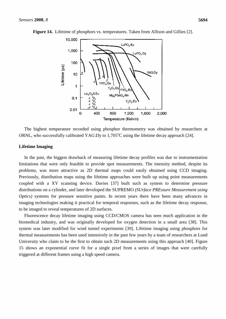
Figure 14. Lifetime of phosphors vs. temperatures. Taken from Allison and Gillies [2].
The highest temperature recorded using phosphor thermometry was obtained by researchers at
ORNL, who successfully calibrated YAG:Dy to 1,705oC using the lifetime decay approach [24].
Lifetime Imaging
In the past, the biggest drawback of measuring lifetime decay profiles was due to instrumentation
limitations that were only feasible to provide spot measurements. The intensity method, despite its
problems, was more attractive as 2D thermal maps could easily obtained using CCD imaging.
Previously, distribution maps using the lifetime approaches were built up using point measurements
coupled with a XY scanning device. Davies [37] built such as system to determine pressure
distributions on a cylinder, and later developed the SUPREMO (SUrface PREssure Measurement using
Optics) systems for pressure sensitive paints. In recent years there have been many advances in
imaging technologies making it practical for temporal responses, such as the lifetime decay response,
to be imaged to reveal temperatures of 2D surfaces.
Fluorescence decay lifetime imaging using CCD/CMOS camera has seen much application in the
biomedical industry, and was originally developed for oxygen detection in a small area [38]. This
system was later modified for wind tunnel experiments [39]. Lifetime imaging using phosphors for
thermal measurements has been used intensively in the past few years by a team of researchers at Lund
University who claim to be the first to obtain such 2D measurements using this approach [40]. Figure
15 shows an exponential curve fit for a single pixel from a series of images that were carefully
triggered at different frames using a high speed camera.

Sensors 2008, 8
5695
Figure 15. Curve fit for a single pixel from a series of images obtained from 8 CCD
detectors [40].
Frequency Domain Lifetime Decay
It is possible to determine decay lifetimes in the frequency domain using a specimen excited by a
continuous wave. The resulting wave will have a different amplitude and phase due to various time
lags of certain luminescent processes. The advantage of this, opposed to a pulsing system, is that
luminescent intensity is expected to higher since the phosphor is being illuminated for 50% of the time.
Figure 16 exemplifies the response for different lifetimes, indicating both changes in phase and
amplitude. Phase lag is proportional to the lifetime and can be determined; an in-depth analysis can be
found in Liu and Sullivan [25]. Burns and Sullivan [41] implemented this technique to map surface
pressure measurements. Temperature measurements using phosphors can also be made, and Allison et
al. [42] reports to have used this technique using blue LEDs.
Figure 16. Phase shifts for different lifetimes.

Sensors 2008, 8
5696
5.3 Risetime Analysis
An investigation by Rhys-Williams and Fuller [43] noted that there are rise times associated with
the response of thermographic phosphors. Their research showed that it was dependant on activator
concentrations. The phosphor under investigation was Y2O3:Eu at room temperature. Ranson later
analysed risetime characteristics in the late nineties and realised that it could be used for detecting
temperature [44].
Ranson et al. [45], notes that the crystal structure of Y2O3:Eu has two sites of symmetry producing
energy levels shown in Figure 17. They note the previous work of Heber et al. [46] who gives evidence
for three potential energy transfers (a,b and c) to level D0. The energy transitions of paths ‘a’ and ‘b’
have been observed to be very fast compared to that of ‘c’ [47]. It is this transition that gives this
phosphor the rise time characteristics.
Figure 17. Energy levels of Y2O3:Eu at symmetry sites C2 ad C3i.
The emission of 611 nm (path d) follows the lifetime decay relation shown previously in section 5.2.
d
t
oeNtN τ−
=)( (10)
where N0, in this case, is the total number of electrons at D0. This is not fixed and depends on the
transition paths ‘a’, ‘b’ and ‘c’. The fast transitions ‘a’ and ‘b’ can be modelled as being instantaneous;
but the transition of ‘c’ is dependant on the decay of electrons from C3i to D0 which decay at
d
t
cic eNtN τ−
=)(3 (11)
Thus, the number of electrons accumulated from path ‘c’ as a function of time is:
−=−=
−−rr
t
c
t
ccc eNeNNtN ττ 1)( (12)
The total number of electrons at Do is then:
−+=
−r
t
cab eNNtN τ1)(0 (13)

Sensors 2008, 8
5697
Combining the equations yields the full characterisation of the decay:
dr
tt
cab eeNNtN ττ−−
−+= 1)( (14)
where τd = lifetime decay, τr is the risetime, Nab and Nc are the number of electrons by transitions a, b
and c, respectively.
The investigations were carried out were carried out using Y2O3:Eu phosphor with approximately
3% Eu concentration. Previous investigations by Rhys-Williams and Fuller [43] noted that rise times
ranged from 60 µs at 5% mole concentration to 320 µs at 0.27% mole concentration. Recent work by
Allison et al. [48] underwent investigations at 0.5% Eu. The results shown in Figure 18 clearly
demonstrate the effects of temperature on risetime, showing a noticeable clear decrease in risetime due
to increasing temperatures. Another temperature related response, that is further discussed section 5.5,
is also shown; there is an increase in luminescence strength due to increasing temperatures. According
to Allison et al. [48], this is due to increased phosphor absorption at the excitation wavelength (337 nm
nitrogen laser).
Figure 18. Risetime variation with temperature. Taken from Allison et al. [48].

Sensors 2008, 8
5698
Figure 18. Cont.
5.4 Line Shift/Width Method
According to Gross et al. [30] temperature can cause the crystal lattice containing the rare-earth to
vibrate creating a changing crystal field that produces a broadening of emission linewidths. Frequency
shift of the spectral lines can also occur due to thermal expansion of the crystal lattice [30]. Both lines
shift variation and broadening can be calibrated to reveal temperature. However, these effects are
usually small. The variation in the line shift at 1,000K is only 3 nm, making the sensitivity very small
and difficult to detect [16]. Kusama et al. [49] utilised this approach for measuring temperature using
Y2O2S:Eu phosphor and the following graph shows variations at -15oC and 72oC. Kusama et al. [49]
suggested quadratic shift according to the equation:
E = A + BT2 (15)
where ‘E’ is the expected energy, ‘A’ is the ground energy at 0K, ‘B’ is a constant, and ‘T’ is the
temperature in Kelvin.
Figure 19. Emmsion lineshift and linewidth variation with temperature [2].
Sensors 2008, 8
5699
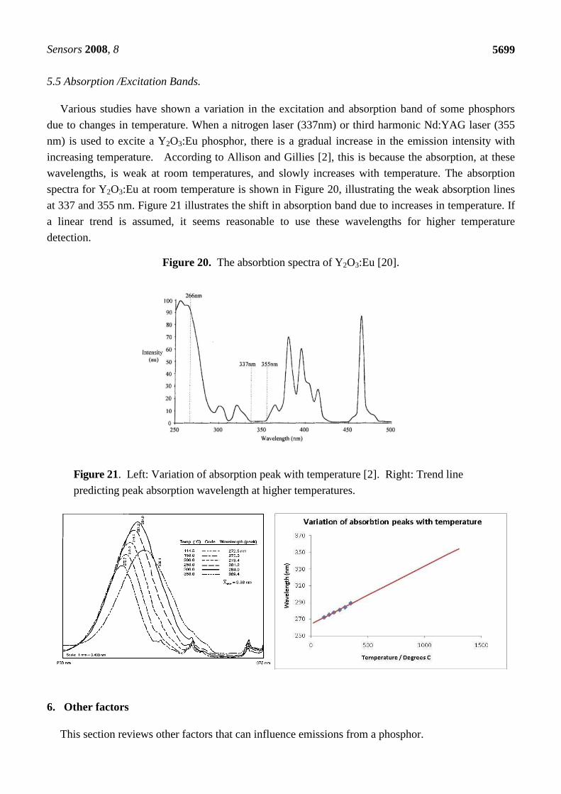
5.5 Absorption /Excitation Bands.
Various studies have shown a variation in the excitation and absorption band of some phosphors
due to changes in temperature. When a nitrogen laser (337nm) or third harmonic Nd:YAG laser (355
nm) is used to excite a Y2O3:Eu phosphor, there is a gradual increase in the emission intensity with
increasing temperature. According to Allison and Gillies [2], this is because the absorption, at these
wavelengths, is weak at room temperatures, and slowly increases with temperature. The absorption
spectra for Y2O3:Eu at room temperature is shown in Figure 20, illustrating the weak absorption lines
at 337 and 355 nm. Figure 21 illustrates the shift in absorption band due to increases in temperature. If
a linear trend is assumed, it seems reasonable to use these wavelengths for higher temperature
detection.
Figure 20. The absorbtion spectra of Y2O3:Eu [20].
Figure 21. Left: Variation of absorption peak with temperature [2]. Right: Trend line
predicting peak absorption wavelength at higher temperatures.
6. Other factors
This section reviews other factors that can influence emissions from a phosphor.

Sensors 2008, 8
5700
6.1 Activator concentrations
It has been shown that the activator concentration affects the temporal decay profile and the
intensity of the emission. Y2O3:Eu concentrations less than 5% leads to strongest lines of shortest
wavelength [16]. Greater concentrations lead to dispersion with no sharp lines being observable. With
increasing concentrations, the energy gap between lines is reduced so electrons reach lower levels from
neighbouring ions by non-radiative means. Allison and Gillies [2] notes that higher activator
concentrations may alter the fluorescent decay so that it follows a multi-exponential rather than a
simple exponential profile, making measurements more difficult to characterise and prone to errors.
As previously discussed, the risetime of the phosphor’s response is also affected by the activator
concentration. Reducing the dopant concentration increases the rise time for Y2O3:Eu phosphor [43].
Not much information is available to see whether this is universally true for other phosphors.
It most applications, it can be assumed that thin coatings of the phosphor exhibit the same
temperature as the surface of interest. However, in some applications, where temperatures are changing
at fast rates, knowledge of the phosphors thermal response is required to properly unfold the
temperature [24]. In YAG phosphors, increasing the dopant concentration reduces the thermal
conductivity. Kontis [32] notes that most 1% dopant YAG phosphors has a thermal conductivity of 4
Wm-1K-1, which is reduced to 2 Wm-1K-1 when the concentration is increased to 3%.
6.2 Saturation Effects
High excitation energies can lead to luminescence saturation. This is where the luminescent
intensity does not change with increasing energy from the source. In fact, above a threshold, there have
been reported cases where luminescent intensity actually decreases with faster decay profiles. There are
a number of explanations for this. The laser beam can induce an increase in temperature [50]; in this
case thermodynamic consideration must be given for these beam related effects. According to Allison
and Gillies [2], this is probably due to the increased probability of two ions being excited in close
proximities. This increases the chances of the energy being transferred from one ion to the other, with
only one photon being emitted instead of two.
6.3 Oxygen quenching / Pressure
Pressure sensitive paints respond to both thermal changes and changes in the level of oxygen.
Thermographic phosphors were originally thought to be independent of oxygen changes. Recent
investigations are challenging this assumption. These investigations are important if phosphors are to
be utilised in areas where the partial oxygen level is likely to change e.g. consumption of oxygen in
combustion chambers.
Feist et al. [51] investigated the oxygen quenching of Y2O3:Eu and YAG:Dy. Volumetric
percentage of oxygen was changed from 21% to 5% by flooding the furnace with nitrogen. No absolute
changes were noted, but the readings resulted in increased uncertainties in temperature measurement.
For Y2O3:Eu, the uncertainties, due to changes in oxygen, were an order of magnitude greater than
uncertainties at fixed concentrations, providing a convincing case for oxygen quenching. However, for

Sensors 2008, 8
5701
YAG:Dy, the uncertainty was the same order of magnitude, and so the results for this case may be
considered as being inconclusive.
A more recent investigation by Brubach et al. [52] showed the effects of various gas compositions
on three different phosphors. The results show that variations in oxygen, nitrogen, helium, carbon
dioxide, water vapour and methane concentrations do not influence the decay time of Mg4FGeO6:Mn
and La2O2S:Eu phosphors. (Figure 22 a,b). These phosphors are only influenced by thermal quenching
and are suitable for environments where changing gas environments are expected. Y2O3:Eu (Figure
22c) however showed high sensitivity to oxygen.
Figure 22. Effects of different gases on the lifetime decay of different phosphors at
different temperatures. Phosphors a) La2O2S:Eu, b) Mg4FGeO6:Mn, c) Y2O3:Eu [52].
b) Mg4FGeO6:Mn
a) La2O2S:Eu

Sensors 2008, 8
5702
Figure 22. Cont.
Apart from pressure causing an increase in partial oxygen levels, there is also evidence that
application of pressure/strain can affect luminescent properties of thermographic phosphors. This
phenomenon is not very well understood but becomes very relevant when extreme pressures are
concerned. The application of pressure can be viewed as the imposition of compressive strain that can
result in changes in both chemical bonds and atomic level orbital configurations. The decay time of
Gd2O2S:Tb decreased by an order of magnitude with application of 2 GPa, while the decay time of
La2O2S:Eu increased by an order of magnitude with application of 3.5 GPa [2].
Although some phosphors may not exhibit oxygen sensitivity, for example La2O2S:Eu [52], they
may possess pressure sensitivity; it is important that both parameters are treated independently.
However, in most flow conditions, it is unlikely that these sorts of pressures will be reached (1GPa =
10,000 Bar). Although, Brubach et al. [52] investigations showed no change in lifetime for La2O2S:Eu
up to a pressure of 10 Bar (1 MPa), the results presented in
Figure 23, illustrates the decrease in decay lifetime at higher pressures (0 – 50 MPa). In very harsh
flows, such as those experienced in gas turbine engines, the maximum pressure is around 50 bar (5
MPa), and the effects of this phenomena may become relevant.
Figure 23. Variation in lifetime decay time of La2O2S:Eu phosphor with increasing pressure [53].
c) Y2O3:Eu

Sensors 2008, 8
5703
Y2O3:Eu phosphor showed sensitivity to oxygen quenching and showed irreversible changes after
the absolute pressure was increased to 6 Bar [52]. According to these findings, Y2O3:Eu, which has
been a very popular choice of phosphor for turbine engine thermometry, is unsuitable for environments
where the pressure and oxygen level is expected to change.
6.4 Impurities and Sensitizers
Impurities in the phosphor can affect luminescence. In a simple case, excitation energy acts directly
on the activator, as shown in Figure 24, which consequently produces radiative emissions with some
energy being lost by other non-radiative means. Impurities in the host material can change atomic
electronic environment experienced by the activators. Transition metal impurities, even at low
concentrations (1 ppm), can decrease luminescence due to them extracting energy that would otherwise
be used to produce radiative emissions. A representation is shown in Figure 25. Since there is a change
in the probability of non-radiative and radiative energy transfers, the decay rate of luminescence is also
expected to be altered.
Figure 24. UV Excitation energy acting directly on the activator.
A UV Excitation
Heat
Luminescence
Figure 25. Interactions between excitation energy, impurities and activator.
A UV Excitation
Heat
Luminescence
I Non radiative
energy transfer
It is possible for the energy transfer to act in the other way. UV radiation on impurities can further
excite the activator by energy transfer. These added impurities are termed sensitizers if their presence
increases luminescence. In some cases, the activator only produces radiative emissions with a sensitizer
is present. (Figure 26– case A). The host lattice can itself act as a sensitizer, for example YVO4:Eu3+.
In other cases, both the activator and the sensitiser can be directly excited, (case B), and the sensitizer
can also be luminescent (case C). The sensitisers could be additional activators, which further
complicates the analysis. Some experiments have revealed that the addition of small amounts of other
activators, such as Dy and Tb or Pr, to Y2O3:Eu decreased the lifetime decay by a factor of 3, with little
change in the quantum efficiency [2].
The energy transfer from the sensitizer to the activator is termed Resonance Energy Transfer (RET).
RET is also possible when the emission spectra of the sensitizer (donor) overlaps the absorption
spectra of the activator (acceptor). The transfer is manifested by the quenching of the donor and the
increased absorption from the activator that consequently results in increased emissions. These
complex mechanisms can be used to explain risetimes and complex multi-exponential decay profiles.

Sensors 2008, 8
5704
Figure 26. Examples of interactions between excitation energy, sensitizer and the
activator.
6.5 Particle size
There have been a number of studies to suggest that lifetime decay and intensity changes with
phosphors particle size. Investigations into nano-crystalline and coarse grain particles of Y2O3:Eu
phosphors reveal that the excited state parabola on the configuration coordinate diagram may be
affected. Konrad et al. [54], explains there is an increasing slope of the excited parabola with reducing
particle size, shown in Figure 27.
Figure 27. Effects of reducing the particle size [54].
S
UV
Excitation
Heat
Luminescence
A
Heat
Energy Transfer
UV Excitation
Case A
Case B
Case C
S
UV
Excitation
Heat
Luminescence
A
Heat
Energy Transfer
S
UV Excitation
Heat
Luminescence A
Heat
Energy Transfer

Sensors 2008, 8
5705
This results in the intersection point between the excited and ground state being increased.
Consequently, the quenching temperature is expected to be higher and the lifetime decays are expected
to last longer. Work by Christensen et al. [55], has shown an increase in lifetime ranging between 436-
598 µs, due to reductions in particle size from 0.42 to 0.11 µm. As different preparation and surface
bonding techniques produce particle sizes, it seem reasonable to assume that the decay lifetime is not
absolute, and therefore it is important that calibration is deployed for that type of preparation or
bonding technique.
7. Bonding Techniques
Adhering the phosphor to the surface of interest is vital for the successful application of phosphor
thermometry. The method should be durable and capable of surviving the exposed environmental
conditions, including the maximum operating the temperature. The method should be inert and should
not change the spectral and thermographic properties of the phosphor. The phosphor coating should
ideally be non-intrusive to the temperature measurement, and therefore provide good thermal contact,
which becomes very important, especially when thermal transients need to be measured. This section
reviews various bonding techniques that have been used at high temperatures.
7.1 Chemical Bonding
This process involves mixing powdered phosphors with chemical bonding agents to create a paint
that can be either brushed or air-sprayed on to a surface. The nature of the binder will depend on the
surface and the operating temperature range. Epoxy binders have a temperature limit that is reached at
a few hundred degrees. Apart from survivability at higher temperatures, chemical binders must allow
transmission characteristics that enable the phosphor to be excited and emissions to be detected.
Chemically bonded phosphors usually require curing by raising the temperature to 700oC and slowly
bringing it back down to room temperature. In the past few years, a variety of commercially available
binders have been investigated [56-58]. Propriety binders manufactured by thermal paints experts at
Rolls-Royce Plc have been successfully tested up to 1,100oC [16]. Some of the higher surviving
commercially available binders include ZYP-ZAP and Coltronics-Resbond, which have shown
survivability and fluorescence detection up to 1,600oC [59]. Table 7 compares some of these binders.
Goedeke et al. [59] notes that although ZYP-ZAP has stronger survivability, the observed fluorescence
is higher in Resbond at 1,500oC.
Problems with chemical binders include the possibility of changing the phosphor’s atomic
configuration, and hence luminescence and thermographic properties. Ideally, chemical binders should
suspend the phosphor without changing atomic properties.
Problems associated at high temperatures include differences in thermal expansion that causes the
paint and substrate to expand at different rates. According to Allison et al. [56], one of the most
challenging surface for bonding is high strength nickel alloy due to high differences in the thermal
expansion coefficients. At high temperatures, this causes the paint to flake off. To increase the thermal
conductivity of the paint, to reduce thermal shock and increase survivability of the paint, tests were
conducted with the addition of MgO2 in the binder.

Sensors 2008, 8
5706
Table 7. Comparison of various high temperature chemical binders [59].
Binder Composition Max temp of both survivability and observed fluorescence. (oC)
Sperex SP115 Silicone Resin About 1,000 Sauerisen thinning liquid
Soluble sodium silicate Water based
1,204
ZYP – BNSL Glassy carbon and magnesium aluminium silicate Alcohol and acetone based
ZYP – HPC magnesium aluminium silicate water based
1,500
ZYP – LK 75% SiO2, 20% K2O, 5% LiO2. Water based
1,100
ZYP-LRC Water based Tested successfully up to 1,400 ZYP – ZAP water-alcohol-based binder Up to 1,600 (YAG:Dy) Coltronics Resbond 791, 792 Silicate Glass,
793 Silica Oxide 795 -Alumina Oxide
up to 1,600
Another problem associated with chemical binders is the effects due to thermal exposure. Figure 28
demonstrates the reduction in emission intensity of Y2O3:Eu phosphor with Resbond 793 binder at
1,400oC after 4 hours of thermal exposure [59]. Similar results were reported by Ranson et al. [60]
using a different chemical binder. The results showed a reduction in intensity to approximately 10% of
their initial value following thermal exposure at 1,200oC for two hours. The reason for this could be
simply due to the paint layer flaking off. Other cases report the paint transitioning to a yellow/brown
colour, and is still unclear whether it is problems with the optical transmission of UV, or the optical
passing of emissions, or a combination of the two that is responsible for the reduction in intensity.
Thermal exposure for long periods may force chemical reactions within the phosphor changing its
characteristics.
Figure 28. Left: emission spectra of Y2O3 phosphor in Resbond binder after thermal
exposure to 1,400oC [59]. Right: Intensity of the peak emission of Y2O3 phosphor after
thermal exposure to 1,200oC [60].

Sensors 2008, 8
5707
Chemical binders allow the use of spray painting. The advantage of this is that large areas of various
sizes and shapes can easily be covered. However, maintaining a uniform surface and controlling the
thickness and roughness can be difficult. Tests indicate a variation in intensity across different test
pieces [61].
The disadvantage of having binder paints is that the minimum coating size that can be produced is
around 10 µm (typical is around 30-60 µm). This is relatively large compared to the vapour deposition
and plasma spraying techniques. Greater thicknesses provide greater thermal gradients between the
phosphor coating and substrate, constituting to a greater error in measurement.
7.1 Vapour Deposition
In this process, a coating is applied by vaporising the phosphor and allowing it to condense on the
surface of interest. There are a variety of ways this can be achieved including electron beam (EB-
PVD), pulsed laser disposition (PLD), chemical vapour deposition (CVD) and RF-frequency
sputtering. No chemical binders are required and therefore there is no interference or problems
concerning optical transmittability of UV and emission wavelengths. The resulting coatings are very
robust and long-lived with fluorescent intensity being constant throughout its life. They can be made
very thin compared to chemical binder paints, and can be finely controlled to have a uniform surface
finish. However, the equipment required to produce these coatings can be very expensive and the
coatings areas are usually very limited.
During vapour deposition, dopant atoms can be situated in a variety of positions and rotations
within the hosts crystal structure and therefore experience a variety of crystal field effects, leading to
weaker and wider spectral emissions. Post annealing is required to realign the ions to restore crystalline
quality and increase luminescent intensity. Allison et al. [2] notes that the high temperatures generated
during vapour deposition can irreversibly break down some phosphors, such as oxy-sulphides, and post
annealing will offer no benefit.
Ranson et al. [60] investigated thin coatings (0.1 µm – 3 µm) produced by RF sputtering and thick
coatings produced by binder paints. They found that emission intensity was related to coating
thickness, up to a certain level. It was shown that 0.7 µm post annealed coatings provided the same
level of intensity as thick coatings (approx 10 µm) produced by chemical binders. These tests were
undertaken for Y2O3:Eu phosphors, and whether this is true for other phosphors is yet to be
investigated.
While thick coating produced by binder paints show declining intensity with thermal exposure,
Ranson et al. [60] showed that thin coatings produced by vapour deposition show no decline in
intensity level. Figure 30 compares shows the variation in luminescent intensity as a function of time
hours of constant thermal exposure at 1,200oC. The results show that the binder paints showed a very
quick decline in intensity, whilst thin coatings produced by vapour deposition showed no change in
intensity.

Sensors 2008, 8
5708
Figure 29. Intensity of thin coatings (0.1 µm-3 µm) after annealing at 1,200oC compared
to thick film (10 µm) and powdered Y2O3:Eu phosphor [60].
Figure 30. The variation in intensity with time (hours) at a constant thermal exposure of
1,200oC for thin coatings (0.1 µm-3 µm) and thick film coatings (10 µm) [60].
7.2 Flame /Plasma Spray
Flame spraying is portable and applicable to objects of diverse geometries, but has a lower impact
velocity than plasma spray [1]. Plasma spraying involves injecting powdered phosphors into an
electrical discharge to liquefy them. The technique allows robust, well-adhered coatings made up from
a multiplicity of solidified droplets [16]. It is usually used to produce thicker films than vapour
deposition methods and can produce coatings exceeding a millimetre. Like vapour deposition,
annealing is also necessary to restore crystalline quality and improve luminescent efficiency.
8. Consideration factors for high temperature measurements
If a system is used at high temperatures, there are certain factors that will make detection difficult.
Many phosphors have reducing intensity whilst exhibiting faster decays. An upper temperature
measurement capability will be reached when the phosphor signals eventually becomes too weak
relative to the noise inherent in the detection system. There is also increasing blackbody radiation that
will eventually become too large making it difficult to separate from the phosphor signal. This
radiation can be predicted using Planck’s radiation law, and Figure 31 illustrates the increasing amount
of radiation as function of wavelength at various temperatures.

Sensors 2008, 8
5709
Figure 31. Distribution of blackbody radiation at different temperatures.
There are a number of approaches that can be adopted to reduce these effects and maximise the
performance of the measurement system. The use of interference filters at the peak emission
wavelengths to filter out the blackbody radiation. The amount of detected radiation is an integration of
both the blackbody radiation and phosphor emission. If a large band filter is used, this radiation can
still be large in comparison to the spiky emission from the phosphor. Figure 32 demonstrates the
amount of blackbody radiation that will be detected if wide and narrow band filters are used. As
shown, the use narrow band filters at the precise peak of phosphor emission can reduce the proportion
of blackbody radiation passing through the filter, yielding better phosphor signal to blackbody radiation
ratios, and hence overall SNR. The downside to this is that there is usually a reduction in the amount of
light passing through to the detector, and therefore a compromise will have be made between the
choice of filter and the system’s ability to detect lowlight level changes. Another complication is that
the phosphor’s peak emission wavelength may vary with temperature, and a very narrowband filter
may not detect the emission at all temperatures. Emission spectra at various temperatures will help
decide the best choice of filter.
Figure 32. Figure to show the amount of background radiation (shaded area) collected
using wide and narrow band filters.
Wavelength Integration using a wide band filter
Inte
nsi
ty
Phosphor emission
Blackbody radiation
Wavelength Integration using a narrow band
filter
Inte
nsi
ty
Phosphor
−=
1)/exp(
12),(
5
2
kThc
hcTW
λλπλ
W is the spectral radiant emittance (Wm-2)
h is the planks constant (Js)
k is the Boltzmann’s Constant (JK-1)
c is the speed of light (ms-1)
λ is the wavelength of light (m);
T is the temperature (K);

Sensors 2008, 8
5710
For any given temperature, the background radiation in is higher at longer wavelengths as seen in
Figure 31. Therefore, it is more effective to use phosphors whose emission wavelength is as low as
possible. Ranson [20] notes that the level of blackbody radiation at 544 nm, the peak emission of
YAG:Tb, is a factor of approximately 5x less than 611 nm, the peak emission for Y2O3:Eu; Allison and
Gillies [2] notes that at 488 nm, one of the peak emissions for YAG:Dy, has an order of magnitude less
blackbody radiation than the peak for Y2O3:Eu. Figure 33 illustrates the intensity that would be
required to maintain the same level of signal to blackbody ratio for each phosphor. The quantum
efficiency of the phosphor at given temperatures must also be considered. Ranson [20] notes that the
strong intensity exhibited by Y2O3:Eu outweighs the advantage of YAG:Tb in terms of blackbody
radiation.
Figure 33. Phosphor intensity (at their peak emission wavelengths) required to maintain
similar signal to blackbody radiation.
Phosphor emissions can be increased if more energy is put into the system, by increasing the
excitation energy. At some point, it is expected that luminescence may saturate, and show no change in
luminescence intensity with increasing energy. Further increases may actually reduce the luminescent
intensity (Section 6.2). In either case, it seems reasonable to find the peak excitation energy that
maximises intensity. In many optical laser systems, this peak is usually not met, and for this reason, a
relatively high energy pulsed light source (usually laser) is more suited.
Apart from the increasing blackbody radiation at higher temperatures, there are other limitations in
temporal approaches, such as the lifetime decay approach, that will cause an upper temperature limit
due to the systems incapability to measure fast decays. The key contributors to this include:
• The limits of data acquisition sampling resolution is reached
• The detectors response time exceed
• Excitation pulse fall times can interfering with the decay time of the phosphor. The energy from a
laser is relatively large and even through high optical density narrow band filters are used to block
any reflected laser light, some light usually leaks through. If the luminescent decay lifetime is on

Sensors 2008, 8
5711
the same order of magnitude as the fall curve of the laser pulse, then it may be difficult to
discriminate between the two. The ideal pulsed light source should have very fast fall times.
9. Emissions Detection
This section reviews various different detectors that are commercially available that can be used for
luminescence detection. It is split into two sections; the first section looks at point detection, and is
followed by imaging.
9.1 Point Detection
For point measurements, there are a number of detectors that can be used, with the main ones being
PMTs, silicon and avalanche photodiodes, and newly developed Si-Photomultipliers. This section
compares these, and the main findings and typical characteristics are highlighted in Table 8.
Photomultiplier Tube (PMT): The PMT has been the most widely used instrument for phosphor
emission measurements. They are very sensitive and responsive, with typical rise and fall times in the
1ns regime. The principle of operation is demonstrated in Figure 34. Photons strike a photo emissive
cathode which emits electrons that are collected at the anode. These electrons are then accelerated
towards a series of additional electrodes (dynodes) that are maintained at a higher potential, generating
additional electrons. This cascading effect creates 105 to 107 electrons for each photon hitting the first
cathode. This amplified signal is finally collected at the anode where it can be measured. PMTs have
large detection areas and can offer a high gain and superior SNR compared to its competitors.
Figure 34. Schematic of a PMT.
Micro channel plate PMT: A MCP-PMT contains an electron multiplier consisting of an array of
millions of glass capillaries fused into a thin disk less than 1mm thick. MCP-PMTs are very fast. The

Sensors 2008, 8
5712
time between the generation of the primary emissive electron at the cathode and the arrival of the
corresponding bunch of electrons at the anode is very small, with response times in the region of 100
picoseconds, making them around 10X faster than conventional PMTs. In the past MCPs were only
available for the detection of VUV, soft X-ray photons and neutrons. They have now been engineered
for visible light detection [62].
Photodiodes: These are semiconductor light sensors. They feature excellent linearity with respect to
incident light, have wide spectral response, are compact, mechanically rugged and have a long life.
Response times typically vary from hundred nanoseconds to a few microseconds, making them slower
than PMTs. However, recent developments enable them to operate at similar bandwidths.
The signal generated by photodiodes is very small relative to noise inherent in the system, resulting
in poor SNR, especially when they are operated at high bandwidths or low light levels. In order to
detect lower light levels, it is usual to increase the gain by increasing the feedback circuit resistor
value. This has unwanted consequences lowering response speed and increasing thermal noise [63]. A
high-speed preamplifier can ensure a wide response speed and lower noise. Avalanche photodiodes
have some intrinsic gain and offer lower noise characteristics than standard electronic amplification,
making them more suited to lower light conditions [63]. The shot noise is often higher; therefore SNR
is not usually improved. However, for low-level detection, gain can be increased to improve SNR,
whilst maintaining response speed, until shot noise reaches thermal noise level [63].
The quantum efficiency of these devices is much higher than that of PMT. However, these detectors
have much smaller detection areas, and it is likely that more light will be lost in collection optics than
gained by quantum efficiency.
Si Photomultipliers (SPM): These are relatively new solid-state devices and have had considerable
amount of research over the past decade. Their performance is superior to that of standard and
avalanche photodiodes in terms of sensitivity, and is approaching that of PMT detectors [64-66]. In
many applications, their performance surpasses that of PMTs. SPM detectors have a number of
advantages over PMTs including: small size, low bias voltage operation, magnetic field insensitivity, a
higher degree of robustness and immunity to damage from high light condition overexposure. The core
of these devices are arrays of APDs operated in Geiger Mode. This technology is thought to eventually
replace conventional PMTs. Further details can be found in the references.
9.2 Imaging
CCD-Charge-Coupled Device: CCDs contain photosensitive elements called pixels that converts
photons into charge. The quantum efficiency for these devices can be as large as 90% for back
illuminated devices. Conversely, the full-well capacity indicates the upper limit can be detected before
electrons spill into neighbouring pixels, smearing the image. In phosphor thermometry, this will be an
important factor, since the level of blackbody radiation becomes increasingly intense at higher
temperatures.

Sensors 2008, 8
5713
Table 8. Comparison of different light detectors.
Standard Photo-diodes
Avalanche Photodiodes APD
Conventional Photo Multiplier Tubes (PMTs)
Micro-channel plate PMT ( MCP-PMTs )
Si Photo-multipliers (SPM, SiPM)
Gain None Low gain (x10-300)
High Gain (106) High Gain (106) Typical = 5 x10⁵
High Gain (106) Much higher gains than APDs. Same region as PMTs.
Bias V High (800V)
High (kV) Low (30V)
Sensitivity Typically < 1 A/W
25 A/W @ 520 nm
30 A/W @ 1,064 nm
40,000 A/W @ 520 nm (SensL)[67]
Sensitivity: 110 uA/lm
Anode sens:
500 A/lm (nominal);
2,000 A/lm (max)
Very high Cathode sensitivity
>1,200 uA/lm (min), 1,500 (typical)
(Burle)[62]
60,000 A/W @ 520 nm (micro)
130,000 A/W @520 nm (mini)
1,000 A/W @ 1,064nm
Response to excess light
Some PIN damaged
Some APDs are damaged
Damage Tolerant
Area Small Small Large diameters- e.g. 46mm.
Arrays are impossible
Small (1x1 mm2)
large areas up to 9mm2 available.
Building larger arrays is possible.
Rise/Fall Times - response
Trise = 0.1 microseconds
Can be operated at 2,000 MHz. (therefore ns)
Rise time: 1 ns. Faster than PMTs.
100 picoseconds
<5ns
Quantum Efficiencies
Higher than PMTs
Higher than PMTs
20-30% at peak >20% at peak 40% @ 520 nm at peak
SNR (signal to noise)
Low
Low.
High
PMTs offer a higher gain, larger detection area and superior SNR compared to APDs
High –
SNR to be similar, and in some cases better than PMTs.
Other notes Robust Robust Fragile, affected by magnetic, electromagnetic interference.
Excellent for pulsed light.
Robust

Sensors 2008, 8
5714
Figure 35. Comparison of different CCD cameras. Pictures taken from Hamamatsu [63].
Frame Transfer (FT) Charge generated in the active area is transferred at high speed to the storage section for each frame; the photosensitive vertical shift register acts as a photo electric converter. The storage section performs signal transfer through horizontal shift registers for each line in the storage section during the horizontal blanking period.
Interline Transfer (IT) These contain a photosensitive section consisting of photodiodes and MOS structure. Vertical shift registers are arranged alongside the photodiode arrays and are comprised of respective output sections that include a horizontal shift register. There is a transfer gate that sits between the arrays and vertical shift transfer. The charge is transferred for all pixels simultaneously. This is then transferred to the horizontal shift transfer for every line.
Full Frame Transfer (FFT) This has the same structure as the frame transfer CCD, except the storage section is removed. The FFT is used in conjunction with an external shutter mechanism. Since the storage is removed, the FFT- CCD can be fabricated to have more pixels or a larger active area per pixel.
Frame Interline Transfer (FIT) These were developed to solve problems of interline CCDs. After the photoelectric charge is transferred to the vertical shift register, the register is clocked and the pixel accumulates the next signal charge. With so many carriers in close proximity, signals leaks into the vertical register causing smears. A storage section was added to reduce this. Now the CCD transfers the signal charge at high speed to the storage section from the vertical shift registers as soon as the signal is received.
Phosphor thermometry using intensity-based methods can be relatively straight forward, where fast
transfers are not required. Fast transfers will be essential for unsteady cases, or when using temporal
approaches. CCDs contain vertical and horizontal registers and an output section. It takes time to read
the charge off the CCD and can be approximated by clocking speeds (10-50 million pixels per second).
Noise is proportional to clocking speeds. Full frame transfer (FFT) devices are optimised for low noise
operation by slowing the scan rate. Figure 35 compares common CCD architectures.

Sensors 2008, 8
5715
CMOS Imagers: Like CCDs, these imagers are made from silicon. Unlike CCDs, each pixel has its
own integrated amplifier. Where CCDs pixels always transfer charge, CMOS pixels converts this to a
voltage, enabling faster clocking speeds and hence frame rates. The relative advantages/disadvantages
are described in Figure 36 and Figure 37. Since CMOS sensors have readout transistors at every pixel,
the active pixel area (fill factor) is reduced. Typical CCD cameras have 5 to 10 times the sensitivity of
CMOS cameras, making them more suited for faint/low light conditions. They compensate for this by
taking longer exposures, and stacking more frames. Binning is also often used to increases sensitivity.
This technique combines the charge from adjacent pixels at the expense of spatial resolution.
Figure 36. Comparison of CCD (left) and CMOS (right) cameras.
Figure 37. Comparison of CCD and CMOS cameras.
Multi-port/Multi-gate CCDs: These devices use multiple amplifiers so that parallel readouts can be
performed. This significantly improve frame rates, and like CMOS cameras fast frame rates up to 10
KHz can be achieved.
Intensified CCD (ICCD): ICCDs utilise an image intensifier coupled to a CCD. They offer high
sensitivity in ultra-low-light-level conditions. Since the intensity is increased, the exposure time can be
reduced and gating methods can be utilized to provide better temporal resolution, allowing the capture
of transient events. These cameras are also suited for lifetime imaging.
Advantages Of CMOS Disadvantages Standard fabrication is lower – on chip integration Low power consumption Random access to pixel regions of interest. Adds flexibility Intra pixel amplification and on chip conversion means faster frame rates.
The fill factor refers to the percentage that is sensitive to light. This is lower in CMOS devices The noise is often more than CCD devices.
CMOS CCD Windowing Yes No Power Low High Integration High Low Speed High Low Blooming No Yes Cost Low High Fill factor Mid/Low High Noise Mid/High Low
Shuttering Difficult Easy

Sensors 2008, 8
5716
Digital APDs/Photon Imagers: Another contender to the ICCD is the digital APD or photon imagers.
Si-Photomultiplier technology has been combined with CMOS technology to form a new generation of
low light cameras currently under development by SensL [67]. The significant difference between this
architecture and traditional CMOS/CCDs is that these devices operate in Geiger mode, allowing them
to be extremely sensitive to individual photons of light. These systems will have the capability to
photon count at the pixel level, making them very sensitive. This could allow for exposure times to be
reduced even further, allowing the capture at finer timescales.
Time delay integration (TDI): This is an effective method for imaging moving objects. Normally, an
image is detected as a signal charge of each pixel. The image must stay fixed during the charge
integration time. If an object is moving, the image can become smeary. The TDI’s CCD has rows of
pixels with charge transfers that are synchronized with the speed of the moving object. This technique
allows clear imaging of objects moving at line rates up to 100kHz [63]. Future improvements of this
technique may prove useful for applications such as high speed turbine blade imaging.
Noise: Noise is unwanted signal that prevents accurate measurements and evaluation. The main
contributors are summarised in Figure 38.
Figure 38. Noise from CCDs.
.
10. Excitation Sources
The energy for excitation can be supplied to luminescent molecules by a variety of ways. Examples
include electromagnetic radiation (lasers and LEDs), particle beams (electrons, neutron, ions) and
electrical current. This section only reviews electromagnetic radiation, focusing mainly on UV lasers.
Fixed pattern Noise (NF). Response variation between pixels caused by differences in sensitivity. Chip defects also contribute to this.
Readout Noise This is electrical noise created from amplifiers and readout circuits. This determines the lower detection limit. The readout noise is usually independent of signal quality but is frequency dependant
Dark shot noise Pixels are subject to thermal effects just like any other electric device. A CCD exhibits a small output even in the dark. (dark current). thermally cooling the device by 5-7K halves the dark current.
Photon Shot Noise Associated with the statistical changes in the number of photons incident of the CCD.
....
ηφAt
vhnphoton =
φ = light power,
hv = photon energy t = exposure time A = Pixel Area η = quantum efficiency
TOTAL NOISE
)(
2222readoutdarkphoton nnnnf ++ +

Sensors 2008, 8
5717
10.1 Pulsed Laser Systems
Nd:YAG Laser Systems: The advantage of temporal approaches, such as the lifetime decay analysis, is
that it is independent of illumination intensity, phosphor concentrations and thickness, and therefore
less prone to errors common in the conventional intensity method. The disadvantage of this method is
that it lacks signal strength, since the excitation light is only available for only fractions of the time.
From the literature, it seems that most researchers have used nitrogen lasers (337 nm) or Nd:YAG
lasers in the third (355 nm) or fourth harmonics (266 nm) to produce high energy pulsed UV light.
These lasers have been an excellent choice for phosphor illumination. The state of this technology has
advanced in the past few decades, and present Q-switched solid state laser system can be expected to
deliver around 500 mJ at 355 nm and 200 mJ at 266 nm with repetition rates of around 20 Hz and
pulse duration of 10 ns [68, 69]. Other newer technologies include diode pumped solid state (DPSS)
Nd:YAG lasers. High powered pulsed laser systems may not be suited for phosphor illumination as
fluence (energy/area) may be too great for the phosphor and issues such as sputtering and the
breakdown of air may become more relevant at energies >30 mJ. However, high-energy laser beams
could easily be expanded to reduce fluence and be used to produce large UV illumination areas suited
for lifetime imaging purposes.
Q switched diode pumped solid state (DPSS) laser: These lasers have laser diodes, instead of flash
lamps, to pump the solid gain medium. They have replaced many flashlamp lasers in many scientific
applications. Pumping efficiencies are greater since the diode’s narrow wavelength is usually optimised
for peak absorption. Flash lamps generate broader wavelengths, with additional light that is not
adsorbed. Typical high energy systems deliver 1 mJ per pulse in the UV range. This is relatively lower
than flashlamp-pumped alternatives. NASA is currently developing the state of the art DPSS laser
system with the goal of transmitting pulse energies greater than 200 mJ in the UV range [70]. DPSS
lasers offer higher repetition rates (500 to 5,000 Hz). Lot-Oriel Group [71] have produced a DPSS
Nd:YAG laser capable of delivering 250 mJ/pulse at 1,064 nm with a repetition rate of 400 Hz and a
pulse width of 800 ps. Assuming a typical reduction in power by an order of magnitude to frequency
triple, or quadruple the laser beam to produce UV wavelengths, this equates to approximately 25
mJ/pulse.
Excimer Lasers: These are gas lasers formed by a mixture of three different gases: a rare earth gas
(e.g. Ar, Kr, Xe), a halogen (either F or Cl), and a bath gas (Ne or He). An advantage of excimer lasers
is that they produce high power pulse outputs directly in UV range, and no frequency
tripling/quadrupling is required, that typically reduces the energy by an order of magnitude. Typical
high energy excimer lasers produce 200 mJ energy/pulse at wavelengths ranging from 157-351 nm
[72]. They typically operate with at a repetition rate of around 500-1000 Hz, with pulse duration near
10 ns. More powerful models, such as Coherent SX series, offer an impressive 1000 mJ/pulse at 300
Hz [73]. According to Junger and Schmidt [74], excimer lasers still remain unchallenged as the only
source laser to deliver high pulse energies and high average powers at UV wavelengths.
In the past, excimer lasers had issues with working lifetimes, laser pulse stabilities and performance.
However, they have vastly advanced in the past few decades with increased gas, tube life and pulse

Sensors 2008, 8
5718
homogeneity [74]. Pulse stabilities have improved from ±12% to ±2%, with a jitter of less than 2ns.
This performance is still slightly lower than Nd:YAG systems with typically stabilities of 1% and jitter
of 0.5 ns. Recent improvements in Junger and Schmidt [74] have reported energy stabilities to have
improved to ±0.5%.
Excimer lasers produce quasi-rectangular beams, typically 8×20 mm, with a near-Gaussian profile
in the short axis, and a super-Gaussian profile in the long axis (Figure 39). Due to the shape and
intensity profile, transformations cannot be made using the same optical systems used for round
Gaussian beams. Most applications require the beam to be modified by homogenizing and then
reshaping the profile to match the application. This can add complexity in the optical system.
Figure 39. Typical rectangular excimer laser profile.
10.2 Continuous lasers/light sources
Continuous lasers and other light sources are suitable for intensity measurements. Pulsing can be
introduced to enable lifetime mode analysis. One way is to use a mechanical shuttering mechanism.
There are limits on how fast these can operate. Previous mechanisms operated in the sub milliseconds
regime, and were considered too slow and unsuitable to detect lifetimes shorter than this. Newer
optical choppers/mechanical shutters can provide sub-microsecond [75] pulses, and now there are a
range of optical shutters (LCDs) that can provide responses faster than this. The problem with
continuous lasers is that the energy per pulse is relatively low. For example, to obtain the same power
as you would from a typical 266 nm 10 ns 10 mJ Q switched Nd:YAG laser pulse, you will need a
continuous laser operating continually with 1 MW of power at that wavelength. Typical high energy
laser systems only operate with average powers of 5 KW. This lack of power from continuous sources
have lead to researchers resorting to high peak power pulsed laser systems, even when they are utilising
the intensity mode [29, 33, 76].
10.3 Fibre Lasers
Fibre lasers are increasing becoming more popular due to increased reliable up-time, beam quality,
reduced running costs and servicing operation. In principal, fibre lasers are similar to DPSS lasers. The
generic design includes laser diodes for pumping; a scheme for coupling the pump energy into the gain
medium; a fibre based resonator configuration with brag gratings instead of mirrors; and a method for
getting rid of excess heat. In a fibre laser, the laser is created directly inside a fibre. Therefore, there is
no need for optical setup that requires the beam to delivered to a target via a series of steering mirrors.
The use of fibre optics opens up areas of application that may have restricted optical access. Fibre

Sensors 2008, 8
5719
lasers eliminate the need to for fibre optic coupling from a conventional laser. Fianium Ltd has recently
created the worlds’ first commercial high-powered 266 and 355 nm UV fibre laser [77]. The system is
capable of producing 1W average power at 100 MHz, with a pulse width of 10 ps. This yields to 0.01
uJ/pulse and a peak power of 1 KW, which is relatively low.
10.4 UV LEDS
Allison et al. [78] reports that high energy UV LEDs could be used to excite phosphors. They can
be used in continuous or pulsed mode. In the pulsed mode, even though they have relatively low
powers, they can be operated with pulse widths to increase the total amount of pulse energy. They have
fall times of a few ns, and have emissions spectra much broader than that of a laser. This may be
absorbed better by the phosphor, and may produce intensities that are of similar magnitude. Newly
developed high powered UV LEDs can produce 450 mW of continuous 380 nm UV light [79]. In
pulsed mode at a pulse width of 1 µs yields to energies of around 0.45 µJ/pulse. This is relatively low
and would therefore be unsuitable for high temperature measurements where blackbody radiation
becomes significant. It may be suitable in applications where relatively low temperatures are
concerned.
LEDs have been very successful and have replaced lasers in many applications including pressure-
sensitive-paints and fluorescence detection for biological purposes [80]. Since the pulse widths can be
finely controlled, the decay lifetime can be determined using the frequency domain approach
highlighted in Section 5.2. A sinusoidal wave using blue LEDs was used to excite the phosphor and
determine lifetime in experiments conduced by Allison et al. [42].
Figure 40. Sinusoidal wave used to excite phosphor. Taken from Allison et al. [42].
11. Survey of recent applications using thermographic phosphor
The use of thermographic phosphors to determine temperature has been successful for a number of
applications. This section briefly surveys some that have been reported in the past few years.
11.1 Impinging Jet Flame Experiment
Kontis et al. [32] investigated a turbulent flame that was impinged onto a 100 µm YAG:Dy
phosphor coated onto an alumina ceramic disc of thickness 0.05 m and diameter of 0.035 m. The

Sensors 2008, 8
5720
intensity ratio method was utilised to map the temperature every 2.5 s for a total of 142.5 s for heating,
and 150 s for the cooling of the plate. The system used was previously shown in Figure 12. The results
show that the maximum temperature (1250K) was attained after 135 s of initial flame impingement.
The temporal variations in the temperature profiles around the centre of the disc is an indication of the
strong and localised effects of hot jets, and the transient heat over the entire disc surface. Kontis et al.
[32] notes that such systems can be used to evaluate the local heat transfer coefficients by using an
appropriate theoretical model of the thermal response to heat flux of the configuration under
consideration.
Figure 41. Centre region radial temperature profiles during a) jet impingement; b)
cooling [32].
Similar transient heating experiments using the intensity ratio method was also undertaken by
Heyes et al. [34]. A ceramic plate was brush-painted with YAG:Dy forming a thickness of 150-200
µm. A Nimonic alloy was coated with YSZ:Dy using plasma spray, producing a thickness of 100 µm.
A Bunsen burner was ignited after 20 s, and was used to heat the rear surface the plates for 60 s. A K-
type thermocouple was mounted on the front surface for comparative analysis. A Nd:YAG laser, with a
pulse energy of 50 mJ, was used to excite the phosphors. Ten pulses were averaged for each
measurement with a sampling period of 1 s.
Results, shown in Figure 42 and Figure 43, for the ceramic plate heating indicate that the front
surface of the plate continued to heat up after the heat was removed. This is to be expected from
ceramic material that has low thermal conductivity. The maximum temperature recorded was at 390K
at 207 s. Results for the Nimonic plate indicate that the maximum temperature was observed at 840K
after 82 s. Thermocouple measurements were in good agreement below 400K (5K difference). At
higher temperatures there were larger differences, highlighting the difficulty of accurately measuring
temperature of hot surfaces using conventional methods. Heyes et al. [34] notes that thermocouples are
expected to under-predict the temperature due to changes in the local temperature caused by
thermocouples acting as a heat sink, imperfect contact, heat loss by thermocouple convention and
radiation, with additional errors caused by the thermocouple junction being above the surface.

Sensors 2008, 8
5721
Figure 42. 2D temperature map for ceramic and nimonic plate at different times. Taken
from Heyes et al. [34].
Figure 43. Temperature history for ceramic and nimonic plates. Taken from Heyes et al. [34].
11.2 After burner experiments
Phosphor thermometry to measure the temperatures of surfaces within operating turbine engines
dates back at least 20 years. Noel et al. [81] proposed such system in 1986. In a study by Saner et al.
[82], optical temperature diagnostics was performed on the afterburner of an Volvo RM12, the engine
used in the Gripen fighterjet. The intensity ratio mode of YAG:Dy was used to map the temperature
inside an afterburner. HPC binder paint was used to attach the phosphor on to the surface of interest. A
355nm Nd:YAG laser was used to excite approx 100 mm2. The phosphorescence signal was sampled
using a stereoscope and an ICCD, allowing the simultaneous imaging of two spectrally filtered images.
The ICCD was gated at 100 µm to suppress background radiation. The images of 455 nm and 493 nm

Sensors 2008, 8
5722
were digital divided to obtain a ratio at each pixel that was processed through a calibration curve to
reveal temperature. Temperature maps were taken at different engine running conditions. Figure 44
shows thermal maps at full afterburner load.
Figure 44. Surface temperature map of a section inside an afterburner [82].
The measurements corresponded well to previous measurements made with thermocouples. This
experiment demonstrates phosphor thermometry could be used in very harsh environments. In addition
to increasing blackbody radiation at high temperatures, another problems that was encountered was
that of flame emissions that overlapped emissions from the YAG:Dy phosphor. The flame emissions
peaked at approx 415 nm. Although, background images were subtracted, it would have been more
beneficial to use phosphors with emission wavelengths that did not interfere with the environment. In
more recent experiments involving afterburner temperatures, the lifetime approach was used to
determine temperature using an 266 nm Nd:YAG laser, a PMT and Mg3FGeO4:Mn phosphor [83].
11.3 Combustor Rig and Film Cooling.
Surface temperature measurements were made in a laboratory combustion rig by researchers at
Imperial College, London [22]. The system was used to assess whether thermographic phosphors could
be used for surface temperature measurements in gas turbines, and to evaluate film cooling. Film
cooling involves the ejection of air over a surface, and is generally used to cool combustor liners,
turbine blades and nozzle guide vanes in gas turbines. It provides thermal protection from high gas
temperatures that usually exceeds the materials melting point, and would otherwise cause failure.
The combustor rig had a quartz window for optical access. Cooling air was directed over the
window by a row of holes to enable it to survive the temperature, while keeping it free from wetting
and carbon build up. The system was first tested using 20 µm Y2O3:Eu paint, prepared by Roll-Royce
Plc, over an underlying TBC of thickness 250 µm. The phosphor was also applied within the
depression of the cooling hole exits. The optical setup was arranged so the lifetime decay response
could be measured using a PMT (Figure 45). A camera lens was used to focus the detection on a single
point, and a traverse was used to successively scan an area of 8mm2 with 128 point measurements.

Sensors 2008, 8
5723
Figure 45. Optical arrangement for combustor measurement [22].
This system evolved and was later modified to simultaneously measure both the intensity ratio and
the decay response of YAG:Dy phosphor, allowing temperature to be determined by two independent
methods [84]. A dichroic mirror was used to split the light equally to two PMTs that had spectrally
different filters capture the relevant wavelengths of 455 nm and 494 nm. A schematic is shown in
Figure 48.
Figure 46. Modified system for simultaneous measurements of the intensity ratio and
lifetime decay response modes [84].
The results (Figure 47) indicate a temperature distribution ranging from 300–600oC, with the
uncertainty reported to be better than 2% [22]. The effects of film cooling holes can be clearly seen,
demonstrating phosphor thermometry’s capability in measuring such phenomena.
Both efficiency (fuel economy) and performance (thrust) can be improved without increasing the
size of the engine if higher turbine inlet temperatures are achieved [85]. However, there are
consequences; a few degrees of operation at over-temperature can result in drastic reductions in blade
life. Therefore, the operating temperature is prescribed by the balance between the benefits of thermal
efficiency at higher temperatures and material stability and life.

Sensors 2008, 8
5724
Figure 47. Results showing the temperature distribution/cooling effectiveness inside the
combustor: (left)Contour map [22]; (Right)Colour thermal map [84].
At the moment, Khalid and Kontis at the University of Manchester are researching into methods of
successfully measuring surface temperatures on both rotating and static components of development
aeroengines using phosphor thermometry. This will eventually help predict heat transfer distributions,
verify the effects of design changes, cooling effectiveness, and aid designers optimise aeroengine
designs to enable higher temperature operation.
11.4 2D surface - Thermal lifetime imaging
Lifetime imaging for thermal measurements using thermographic phosphors has been intensively
used by a team of researchers at Lund University. They claim to be the first to obtain such 2D
measurements [40]. A high speed framing camera (Imacon-Hadland), containing an eight faced prism
is used to split light to eight independent intensified CCD cameras, where the exposure time and time
separation between images can all be precisely configured.
Figure 48. Architecture of the framing camera, showing the eight faced prism splitting the
light equally to eight ICCD cameras [86].

Sensors 2008, 8
5725
Figure 48 shows a schematic of the framing camera. Using these images, an exponential curve can
be fitted for each pixel, and evaluated against a calibration curve (Figure 49). This produces a complete
2D thermal map that was determined using lifetime decay analysis.
Figure 49. Left: Curve fit for each pixel from intensities integrated from 8 CCD detectors;
Right: Schematic for temperature measurement. Pictures taken from [40].
The group have obtained 2D surface measurements on low density fibre boards covered with
Mg4FGeO6:Mn phosphor. Burning alcohol was used to heat the sample because it generates less soot
that could interfere with measurements.
Figure 50. Temperature measurements during flame spread. 2D surface temperature
measurement of low density fibreboard (LDF) [86].

Sensors 2008, 8
5726
The radiation energy was 24 mJ/pulse which was expanded to an area of 100 cm2 yielding a fluence
of 0.25 mJ/cm2. The results obtained showed a standard deviation of ±5K (less than 1%) at
temperatures between 680-780K [40]. Recent experiments involved measurement of combustible and
non-combustible surfaces using both the intensity ratio and lifetime imaging modes [86]. Figure 50
shows thermal temperature maps during a flame spread experiment at various times.
11.5 Surface Temperature Measurements of decomposing materials
The surface temperature is a key parameter for modelling the decomposition of solid materials. It
has a strong influence on the heat flow into and out of the material, and also determines the ignition
temperature. Omrane et al. [87] used phosphor thermometry for surface temperature measurements in
pyrolysis studies. Pyrolysis is the chemical decomposition of organic materials by heating in the
absence of oxygen or any other reagents. According to the authors, accurate measurement using
conventional methods prove to be problematic. Thermocouples and thermistors require direct contact,
and may suffer heat losses and induce catalytic effects. Pyromerty can be difficult because emissivity
of the surface may not be known and may be changing during the investigation.
Figure 51. Schematic and results from the pyrolysis study for birchwood [40].
Phosphor particles were deposited on the material under investigation and were placed inside a high
temperature reactor that was pre-stabilised at a temperature of 733K [40]. A 266 nm Nd:YAG laser
was used to excite the sample with subsequent emissions collected by a PMT, ICCD and a
spectrograph, for both temporal and spectral analysis. A schematic is shown in Figure 51. The results
show that the surface temperature increased to reach the temperature of the reactor.
In later work, pyrolysis on construction materials were studied. These included low-density fibre
boards (LFB), medium fibre boards (MDF), particle board (PB) and polymethylmetharcrylate (PMMA)
[87]. Cubic samples (5 mm3) were doped into Mg4FGeO6:Mn phosphor that was dispersed in ethanol
or toluene. The samples were dried at 95oC and inserted through an air cooled fall tube onto to a
holder. This was connected to a balance to monitor weight of during the investigation. A molecular
beam mass spectrometer was used to monitor gas composition and ensure oxygen levels stayed below
0.1%.

Sensors 2008, 8
5727
Figure 52. Schematic to study the pyrolysis of construction materials [87].
The rapid pyrolysis of construction materials was successfully monitored using phosphor
thermometry. The results covered a temperature range of 300-600oC. This covers pyrolysis initiation
and completion for most construction materials during typical fire spread situations. The results are
another demonstration of phosphor thermometry for detailed temperature measurements during these
complex combustion-related situations where common techniques fail.
11.6 Internal Combustion Engine valve/piston temperature measurement
Temperature measurement of internal component surfaces enhances understanding of the processes
inside the combustion engine. Armfield et al. [88], cited in Allison et al. [53], reports the use of
thermographic phosphors for temperature measurements of an intake value and a piston.
Figure 53. Schematic for intake value measurements.
For the intake value experiments, LaO2S:Eu phosphor was coated on the stem-side of the value. A
nitrogen laser was delivered through a 1mm optical fibre accessed through the head of the car. The

Sensors 2008, 8
5728
same fibre was used to direct the luminescent emissions to a PMT. The lifetime decay response was
used to determine temperature. A schematic is shown in Figure 53. For piston measurements, a quartz
window was used to gain direct optical access as shown in Figure 54.
Figure 54. Schematic for piston measurements [53].
The results shown in Figure 55 indicate show that in both cases, there is a rapid increase in
temperature and is followed by a slower steady increase.
Similar temperature measurements of the intake and exhaust values of an optically accessible
laboratory engine was conducted by Omrane [86]. Measurement would increase the understanding of
fuel evaporation process when it is in contact with high temperature surfaces. In the investigation, the
engine was operated at 1,200 RPM using gasoline and iso-octane fuel.
Figure 55. Results for piston and intake value experiments [53].
A thermographic phosphor was bonded onto the values using commercial binder. A fourth harmonic
Nd:YAG (266 nm) was used to excite the phosphor through a quartz window. The emission signals
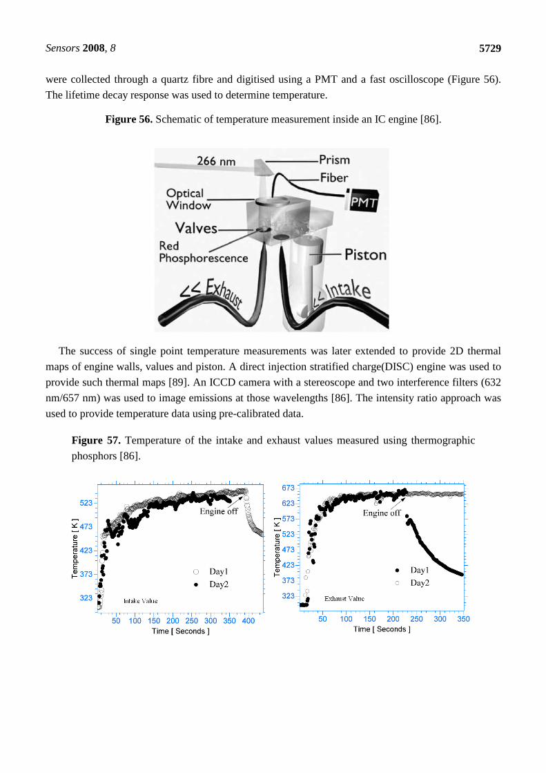
Sensors 2008, 8
5729
were collected through a quartz fibre and digitised using a PMT and a fast oscilloscope (Figure 56).
The lifetime decay response was used to determine temperature.
Figure 56. Schematic of temperature measurement inside an IC engine [86].
The success of single point temperature measurements was later extended to provide 2D thermal
maps of engine walls, values and piston. A direct injection stratified charge(DISC) engine was used to
provide such thermal maps [89]. An ICCD camera with a stereoscope and two interference filters (632
nm/657 nm) was used to image emissions at those wavelengths [86]. The intensity ratio approach was
used to provide temperature data using pre-calibrated data.
Figure 57. Temperature of the intake and exhaust values measured using thermographic
phosphors [86].

Sensors 2008, 8
5730
Figure 58. Temperature images of the intake(upper quadrant) and exhaust values(lower
quadrant) measured using thermographic phosphors [86].
Both results, shown in Figure 57 and Figure 58 illustrate the exhaust values start to heat up earlier
than the intake value, and also reaches a higher temperature. This is due to new fresh air entering the
intake value allowing it to be cooled. In addition, the exhaust value also experiences burned gases
from the combustion chamber that heat up the value [76].
11.7 2D Gas Temperatures
The thermographic phosphor method has recently been used to measure gas temperatures.
Hasegawa et al. [36] investigated the intensity ratio of YAG:Dy for such measurements with the
ultimate aim of measuring the gas temperatures in an operational engine.
Figure 59. Experimental setup for temperature measurement for steady gas flow [36].
A static calibration, followed by a steady flow validation, was conducted before actual engine tests.
In the calibration procedure, an imaging stereoscope and two band pass filters were used in front of an
ICCD. The lifetime of the phosphor was also detected using a PMT to optimise the gate times for the

Sensors 2008, 8
5731
ICCD. In gas flow validation experiments, phosphor-seeded air was passed through a 10 mm diameter
exit at a velocity of 80 cm/s. A temperature-controlled heater was used to heat the flow to 573K 15 mm
below the tube exit. A schematic is shown in Figure 59.
Figure 60. Gas temperature caparisons between thermocouple readings, lifetime method
and intensity ratio method [36].
Figure 60 compares three different methods of measurement. The thermocouple readings were
lower, as expected, since its intrusiveness perturbs the flow field with ambient room temperature,
decreasing its temperature. According to Hasegawa et al. [36], the fluctuations in the intensity ratio
method are mainly due to heterogeneity of gas seeding, causing a temperature error of around 5%.
During engine tests, a four cylinder diesel engine running at 1,200 RPM was used. A 355 nm
Nd:YAG laser was used at 80 mJ/pulse and a homebuilt seeding device was used to obtain
homogenous seeding. According to the authors, the intrusion of the phosphor caused an average drop
in temperature by 2%. It was shown that phosphor thermometry could be used to measure temperatures
of un-burnt gas flows. In turbulent combustion conditions inside the engine, phosphor temperature data
agreed well within 5% error with the thermodynamic calculated data. However, chemi-luminescence
effects caused measurements to be restricted after 10o after top dead centre. Further details on this can
be found in the reference.
11.8 Droplets and Spray thermography
Laser induced phosphoresce from thermographic phosphors was used to measure temperature of
single falling droplets [90]. The droplets were excited using 266 nm Nd:YAG. The resulting emissions
were evaluated spectrally, using a stereograph and Mg3FGeO4:Mn phosphor; and temporally, using a
PMT and La2O2S:Eu phosphor. Phosphor (1%, by weight) was added to the liquid under investigation.
A Nd:YAG laser was triggered when a droplet crossed a He-Ne beam. The setup is shown in Figure

Sensors 2008, 8
5732
61. The droplets were approx 3-4 mm in diameter. The temperature of the liquid was controlled using a
thermocouple and heating wires around the container.
Figure 61. Experimental set up for droplet temperature measurement using thermographic
phosphors [86].
The results for both spectral and temporal methods are presented in Figure 62. The phosphor
determined temperatures correspond well with the thermocouple readings from inside the tank. The
thermocouple readings do not take into consideration the cooling and heat exchange to the surrounding
air after it has left the nozzle.
Figure 62. Temperature comparisons from thermocouple values, predicted model values,
and actual phosphor measurements [86].

Sensors 2008, 8
5733
To compensate for this, a model from Kinciad and Longley [91] was used. The results from the
phosphors agreed very well to this with deviations less than 1%. Although the temperature of the
droplets is of relatively low temperature, it does demonstrate the principle and may be used to measure
much higher temperatures.
The same methodology was extended to form 2D thermal measurements of droplets using fast
framing ICCD cameras and decay lifetime imaging. The temperature at each pixel was evaluated using
calibration procedure of lifetime against temperature. The technique was first applied to free falling
water-based droplets, then to a suspended droplet in an ultrasonic levitator [92], and later to sprays
[93]. Figure 63 illustrates some example of results that were obtained. Brubach et al. [94] also
performed 2D spray and droplet thermometry using the intensity ratio approach using a
Mg4GeO5.5F:Me thermographic phosphor. Further details can be found in the references.
Figure 63. Examples of 2D droplet (left) and spray (right) thermometry using lifetime
imaging [86].
11.9 Supersonic Combustor experiments
Kontis [33] investigated surface transfer measurements inside a supersonic combustor. The
experiment was conducted on a blown-down design supersonic wind tunnel. The run time was
approximately 8 s with 4 s of steady state flow conditions at nominal values. The schematic of the test
section can be seen in Figure 64 with further details explained in the reference. Hydrogen fuel was
injected through a slit located along the back surface of the step. Two alumina ceramic pieces were
secured using a high temperature adhesive both upstream and downstream of the step. These were
coated with a thin layer (<50 µm) of YAG:Dy. The total thickness of the phosphor + ceramic was
approx 0.01 m. Frequency tripled Nd:YAG laser (355 nm) was used to excite the phosphor after 1 s,
allowing time for hydrogen fuel combustion. Emission profiles were then recorded every second using
the intensity ratio method.
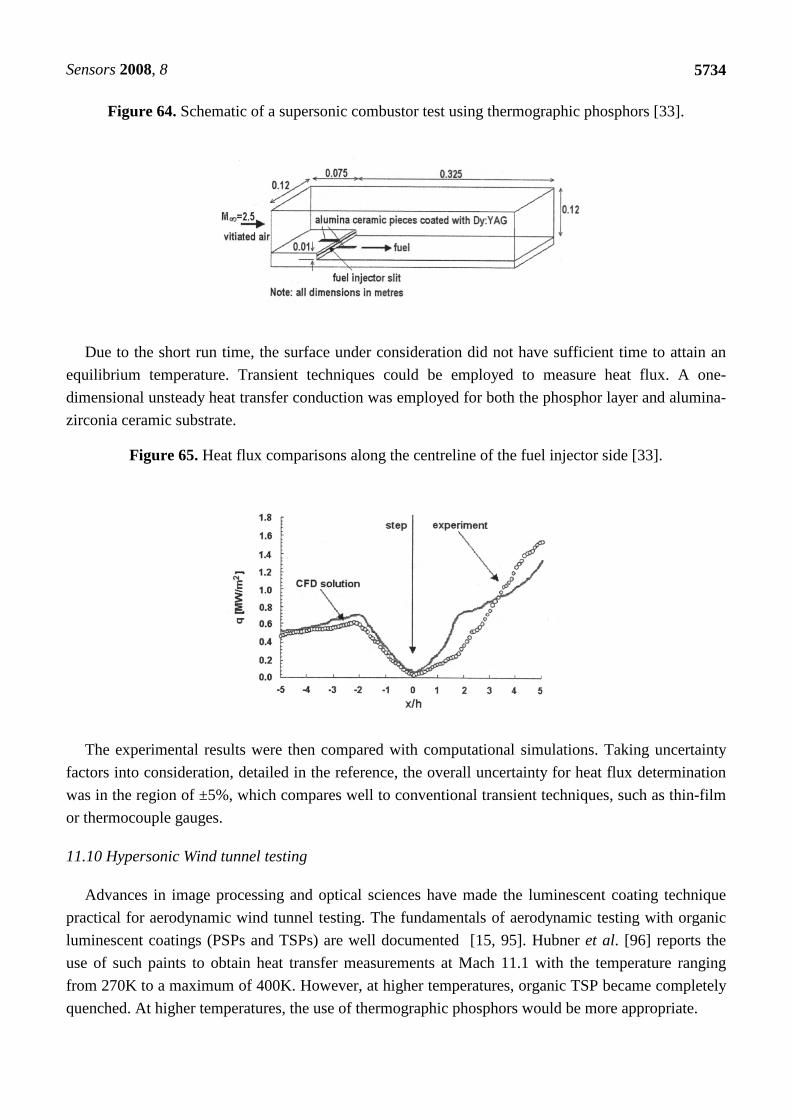
Sensors 2008, 8
5734
Figure 64. Schematic of a supersonic combustor test using thermographic phosphors [33].
Due to the short run time, the surface under consideration did not have sufficient time to attain an
equilibrium temperature. Transient techniques could be employed to measure heat flux. A one-
dimensional unsteady heat transfer conduction was employed for both the phosphor layer and alumina-
zirconia ceramic substrate.
Figure 65. Heat flux comparisons along the centreline of the fuel injector side [33].
The experimental results were then compared with computational simulations. Taking uncertainty
factors into consideration, detailed in the reference, the overall uncertainty for heat flux determination
was in the region of ±5%, which compares well to conventional transient techniques, such as thin-film
or thermocouple gauges.
11.10 Hypersonic Wind tunnel testing
Advances in image processing and optical sciences have made the luminescent coating technique
practical for aerodynamic wind tunnel testing. The fundamentals of aerodynamic testing with organic
luminescent coatings (PSPs and TSPs) are well documented [15, 95]. Hubner et al. [96] reports the
use of such paints to obtain heat transfer measurements at Mach 11.1 with the temperature ranging
from 270K to a maximum of 400K. However, at higher temperatures, organic TSP became completely
quenched. At higher temperatures, the use of thermographic phosphors would be more appropriate.

Sensors 2008, 8
5735
NASA Langley Research Centre has been using the relative-intensity two-colour phosphor
thermography system for at least 15 years. It has become a standard technique to measure temperature
and flux. An UV illuminated phosphor coated model is exposed to the wind tunnel flow. Subsequent
emissions from two wavelengths are observed and converted to surface temperature maps using pre-
calibrated data. With temperature maps acquired at different times during the run, global heat transfer
images can be computed, assuming an one-dimensional semi-infinite heat conduction model. Scaled
hypersonic models of X-33 [97], X-34 [98], X-38 [99, 100] and X-43 [101] have all been tested in
wind tunnels using phosphor thermometry at Mach 6 and 10 in air, and some have been tested at Mach
20 in Helium [97]. Further details can be found in the references.
According to NASA, the primary advantage of thermographic phosphors is the global resolution of
the quantitative heat transfer data which can be used to identify heating footprints of complex, 3D flow
phenomena, including transitional fronts, turbulent wedges and boundary layer vortices, that are
extremely difficult to resolve using discrete measurement techniques. In addition, the technique does
not need corrections that are required for infrared thermometry.
According to Hovarth et al. [97], measurement accuracy via phosphor thermometry is believed to
better than around 8%, and the overall experimental uncertainty in heating data due to all factors is
estimated to be around 15%, including uncertainties in the in the thermo-physical properties of the
ceramic model. This is somewhat similar to that of thin films. Repeatability was found to be generally
better, around 4% [100]. Merski [102] notes that the total uncertainties associated with the phosphor
technique is shown to be approximately 7–10% in NASA’s 31-Inch Mach 10 Tunnel and 8–10% in the
20-Inch Mach 6 Tunnel. A comparison with thin film measurements showed phosphor data to be
within 7% and agreed better than CFD predictions. Figure 66 illustrates an example of the match
between experimental phosphor data and predicted CFD data.
The phosphor technique provides a wealth of information critical to the design of thermal protection
systems for applications involving engine design, re-entry vehicles, missiles and supersonic and
hypersonic transport. Further research and work with phosphor thermometry at hypersonic speeds is
planned at the University of Manchester in the near future.
Figure 66. Comparison of extrapolated turbulent experimental data with predicted CFD
data. Taken from Horvath et al. [100].

Sensors 2008, 8
5736
Figure 66. Cont.
11.11 Smart Thermal Barrier Coatings
Thermal Barrier Coatings (TBCs) provide thermal protection. They are usually found in very hot
regions of a gas turbine engine. TBCs consist of a thin bond coat and an insulating layer, usually YSZ.
They have a thickness in the order of 250 µm. TBC can be modified to behave like thermographic
phosphors[103], exhibiting temperature dependable properties. The advantage of this is that no
additional phosphor layers are required for temperature measurement. This concept was first proposed
by Choy, Feist and Heyes [104].
YSZ:Eu and YSZ:Dy have been investigated both in powdered form and various forms of vapour
depositions. Powdered YSZ:Eu response was observed with a dynamic range of 50-800oC with a
repeatability of ±0.1% using the lifetime method. YSZ:Dy was investigated using the intensity ratio
method and was calibrated through a temperature range of 300-900K. This showed a repeatability of
data around ±0.6% [34].
Using this methodology, it is possible to measure the temperature of the TBC. However, at high
temperatures, there is a huge temperature gradient across the TBC, with temperatures being 200oC
higher than that of the actual substrate. Figure 67 illustrates typical temperature variation across a TBC
that is attached to a turbine blade experiencing high temperature flows. The actual substrate
temperature is important for designers because it is this that determines material failures.
Thermographic TBC may be created from multi-laminar construction layers as illustrated in Figure
68. With this arrangement, discreet points in the coating could be measured, including the temperature
of the bond coat. The actual doped YSZ could be sandwiched in between the undoped YSZ allowing
temperature measurement at various distances through the TBC. This information could be used to
determine the health of thermal barrier coatings. Southside Thermal Sciences, UK are further
developing this concept.

Sensors 2008, 8
5737
Figure 67. Temperature variation across the section of a TBC deposited on a substrate [105].
Figure 68. Phosphor thermometry at different distances though a YSZ-TBC.
11.13 Galvanneal Process
The protective galvanneal process involves the dipping and heating of steel into molten zinc until
the iron and zinc atoms form an alloy on the surface. The metals surface temperature may vary in the
furnace, causing product quality and non-uniformity problems. Researchers at the ORNL developed a
measurement system, based on the lifetime decay mechanism of phosphor thermometry to strictly
control surface temperature, enabling the production of uniform, high-quality galvanneal steel [106].
The system, shown in Figure 69, includes a computerized phosphor-deposition device that is used to
dust phosphor powder on the steel sheet. A portable nitrogen laser (377 nm, 0.3 mJ/pulse, 30Hz) is
used to excite the phosphor, and subsequent emissions are detected and analysed in real time to
Bond Coat (Pt)
Undoped YSZ
Doped YSZ
Undoped YSZ
Substrate – Ni Alloy
TBC
Doped Layer can be at any distance above the bond coat
Excitation through TBC
Emission through TBC

Sensors 2008, 8
5738
evaluate and control the surface temperature by adjusting furnace settings. In 1998, the system was
successfully installed and tested at Bethlehem Steel's facility in Burns Harbor, Indiana.
Figure 69. Schematic of the Galvanneal temperature measurement system [107].
12. Conclusions
The idea of using phosphors for temperature measurements dates back to 1938. The capture and
analysis of fast pulses required very expensive and sophisticated instrumentation. Over the past few
decades there have been many advances in science and technology that allowed the phosphor
technology to flourish and reach newer application areas. The fundamental principles of luminescence
and phosphor thermometry were presented and various intensity, temporal and spectral approaches
were discussed. Various other factors affecting the luminescence process were also discussed.
Phosphor thermometry is largely immune from errors common in pyrometry, such as emissivity and
sensitivity to stray light. However, it requires bonding to the surface of interest, causing intrusiveness
that can become relevant in complex situations. There is also an upper temperature limit due to
increasing blackbody radiation and generally reducing phosphor signals at higher temperatures.
Recent developments and applications demonstrate phosphor thermometry being very flexible and
successful in measuring temperatures in many different applications areas ranging from gas turbine
measurements, internal combustion engine piston and value measurements, pyrolysis studies, to
supersonic and hypersonic wind tunnel experiments. Apart from surface measurements, the technique
has also been extended to measure temperatures of droplets, sprays and gases.
Acknowledgements
The authors would like to thank the Engineering and Physical Sciences Research Council (EPSRC)
and Rolls-Royce Plc, especially Colin Bird, for technical advice and financial support.

Sensors 2008, 8
5739
References
1. Kontis, K. A review of some current research on pressure sensitive and thermographic phosphor
techniques. The Aeronautical Journal 2007, August, 3162, 495-508
2. Allison, S.W.; Gillies, G.T. Remote thermometry with thermographic phosphors: Instrumentation
and applications. Review of Scientific Instruments 1997, 68, 7, 2615-2650
3. Arpiarian, N. The Centenary of the Discovery of Luminescent Zinc Sulphide. Proceedings of the
International Conference on Luminescence. Budapest. 1966. pp. 903-906.
4. Harvey, E.N. A History of Luminescence From the Earliest Times Until 1900, J.H., Furst
Company, Baltimore, Maryland, 1957.
5. Leverenz, H.W., An Introduction to Luminescence of Solids, Dover Publications, New York,
1968.
6. Larach, S.; Hardy, A. Cathode-Ray-Tube Phosphors: Principles and Applications. Proceedings of
the IEEE 1973, 61, 7, 915-926
7. Keller, P.A. The 100th Anniversary of the Cathode-Ray Tube. Information Display 1997, 12-16
8. Yen, W.M.; Shinoya, S.; Yamamoto, H., The Phosphor Handbook - Second Edition, Taylor &
Francis Ltd, CRC Press, Boca Raton, Florida, 2006.
9. Nuebert, P. Device for indicating the temperature distribution of hot bodies - US Patent No.
2,071,471. 1937, 10. Czysz, P.A.; Dixson, W.P. Thermographic heat transfer measurement. Instrumentation Control
Systems 1968, 41, 71,
11. Czysz, P.A.; Dixson, W.P. Quantitative Heat Transfer Measurement Using Thermographic
Phosphors. SPIE 1969, 7, 3, 77-79
12. Wickersheim, K.; Alves, R. Ind. Res. Dev 1979, 21, 82,
13. Cates, M.R. Applications of pulsed laser techniques and thermographic phosphors to dynamic
thermometry of rotating surfaces. ICALEO 84: Proceedings: Inspection, Measurement and
Control. 1984. 45, pp. 4-10.
14. Alaruri, S.; McFarland, D.; Brewington, A.; Thomas, M.; Sallee, N. Development of a fiber-optic
probe for thermographic phosphor measurements in turbine engines. Optics and Laser
Engineering 1995, 22, 17-31
15. Bell, J. H.; Schairer, E. T.; Hand, L. A.; Metha, R. D. Surface pressure measurements using
luminescent coatings. Annual Review of Fluid Mechanics 2001, 33, 155-206
16. Heyes, A. L. Thermographic Phosphor thermometry for gas turbines. Advanced Measurement
techniques for aeroengines and stationary gas turbines. Von Karmen Institute for fluid dynamics.
March 1-5. 2004.
17. Turro, N. J., Modern Molecular Photochemistry, Benjamin/Cummings, Menlo Park, CA, 1978.
18. Sant, Y. L.; Merienne, M. C. Surface Pressure Measurements by Using Pressure-Sensitive Paints.
Aerospace Science Technology 2005, 9, 3, 285-299
19. Royer, C. A. Approaches to teaching fluorescence spectroscopy. Biophysical Journal 1995, 68,
1191-1195
20. Ranson, R. M., PHD Thesis - Investigation into thermographic phosphors, Nottingham Trent
University, 1999.

Sensors 2008, 8
5740
21. Fonger, W.H.; Struck, C.W. Eu3+ 5D Resonance Quenching to the Charge Transfer States in
Y2O3S, La, La2O2S, LaOCl The Journal of Chemical Physics 1970, 52, 12, 6364
22. Feist, J.P.; Heyes, A.L.; Seefeldt, S. Thermographic phosphor thermometry for film cooling
studies in gas combustors. Proceedings of the Institution of Mechanical Engineers, Part A:
Journal of Power and Engineering. 2003, 217, 2, 193-200
23. Kerr, C.; Ivey, P. An overview of the measurement errors associated with gas turbine aeroengine
pyrometer systems. Measurement Science Technology 2002, 13, 837-881
24. Cates, M.R.; Allison, S.W.; Jaiswal, S.L.; Beshears, D.L. YAG:Dy and YAG:Tm fluorescence to
1700oC. The 49th International Instrumentation Symposium - The Instrumentation, Systems, and
Automation Society. Orlando, Florida. May. 2003.
25. Liu, T.; Sullivan, J.P., Pressure and Temperature Sensitive Paints, Springer, Berlin, 2005.
26. Bizzak, D.J.; Chyu, M.K. Use of a laser induced fluorescence thermal imaging system for local jet
impinging heat transfer measurement International Journal of Heat and Mass Transfer 1995, 32,
2, 267-274
27. Chyu, M.K.; Bizzak, D.J. Surface temperature measurement using a laser induced fluorescence
thermal imaging. Journal of Heat Transfer 1994, 116, 263-266
28. Chyu, M.K.; Hsing, Y.C. The use of a thermographic phosphor imaging system for simultaneous
measurement of film cooling effectiveness and heat transfer coefficients. Proceedings of the
international gas turbine and aeroengine congress and exposition. Birmingham. 1996.
29. Feist, J.P.; Heyes, A.L. The characterisation of Y2O2S:Sm powder as a thermographic phosphor
for high temperature applications. Measurement Science Technology 2000, 11, 942-947
30. Gross, G.P.; Smith, A.A.; Post, M.E. Surface Thermometry by laser induced fluorescence. Review
of Scientific Instruments 1989, 60, 12,
31. Carnall, W.T.; Rajnak, K. Electronic energy levels in the trivalent lanthanide aquo ions. Journal
of Chemical Physics 1968, 49, 4424-4442
32. Kontis, K.; Syogenji, Y.; Yoshikawa, N. Surface thermometry by laser induced fluorescence of
Dy3+:YAG The Aeronautical Journal 2002, 106, 1062, 453-457
33. Kontis, K. Surface Heat transfer measurements inside a supersonic combustor by laser induced
fluorescence. Journal of Thermophys Heat Transfer 2003, 17, 3, 320-325
34. Heyes, A.L.; Seedfeldt, S.; Feist, J.P. Two-colour phosphor thermometry for surface temperature
measurement Optics and Laser Technology 2006, 38, 4-6
35. Feist, J.P.; Heyes, A.L.; Seefeldt, S., in 11th International symposium on Application of Laser
Techniques to Fluid Mechanics, Lisbon, Portugal, 2002. 36. Hasegawa, R.; Sakata, I.; Yanagihara, H.; Johansson, B.; Omrane, A.; Alden, M. Two-
dimensional gas phase temperature measurements using phosphor thermometry. Applied Physics
B - Laser and Optics 2007, 88, 291-296
37. Davies, A.G. Recent developments in pressure sensitive measurements. Proceedings of wind
tunnels and wind tunnel tests technique Conference. Cambridge. 1997.
38. Szmacinski, H.; Lakowicz, J.R. Fluorescence lifetime based sensing and imaging. Sensors and
Actuators B 1995, 29, 16-24

Sensors 2008, 8
5741
39. Holmes, J.W. Analysis of radiometric, lifetime and fluorescent lifetime imaging for pressure
sensitive paints. The Aeronautical Journal 1998, April, 189-194
40. Omrane, A.; Ossler, F.; Alden, M. Two-Dimensional Surface Temperature Measurement of
burning materials. Proceedings of the Combustion Institute. 2002. 29, pp. 2653-2659.
41. Burns, S.; Sullivan, J.P. The use of pressure sensitive paints on rotating machinery. Proceedings
of the16th International Congress on Instrumentation in Aerospace Simulation Facilities
(ICIASF), IEEE. Wright-Patterson Air Force Base, Dayton, USA. 1995. pp. 32.1-32.14.
42. Allison, S.W.; Beshears, D.L.; Cates, M.R.; Paranthaman, M. LED-induced fluorescence
diagnostics for turbine and combustion engine thermometry. Proc. SPIE. International Society for
optical engineering 2001. 4448, pp. 28-35.
43. Rhys-Williams, A.T.; Fuller, M.J. The use of a computer controlled luminescence spectrometer in
a study of the time resolved emission of trivalent europium in yttrium oxide. Computer Enhanced
Spectroscopy 1983, 1,, 145,
44. Ranson, R.M.; Thomas, C.B.; McClean, I.P. Phosphor thermography sensing using rise time
analysis - UK PATENT NO: GB 9723018.9. 1997, 45. Ranson, R.M.; Evangelou, E.; Thomas, C.B. Modelling the fluorescent lifetime of Y203:Eu.
Applied Physics Letters 1998, 72, 21, 2663-2664
46. Heber, J.; Hellewege, K.H.; Kobler, V.; Murmann, H. Energy level and interaction between Eu3+
ions at lattice sites of symmetry C2, and C3i in Y203. Zeitschrift für Physik 1970, 114, 237
47. Hunt, R.B.; Pappalardo, R.G. Fast excited state relaxation of Eu-Eu pairs in commercial Y2O3
phosphors. Journal of Luminescence 1985, 34, 133-146
48. Allison, S.W.; Goedeke, S.M.; Cates, M.R.; Hollerman, W.A.; Eldridge, J. I.; Bencic, T. J.
Fluorescence Rise Time Measurements for High Temperature Fluorescence-Based Thermometry.
Oak Ridge National Laboratories Report 2005, R05-123055; USDOE,
49. Kusama, H.; Ojar, J.S.; Taisuke, Y. Lineshift Method for phosphor temperature measurements.
Japanese Journal of Applied Physics 1976, 15, 12, 2345
50. Imanaga, S.; Yokono, S.; Hoshima, T. Luminescence Saturation Effects in Y2O2S:Eu. Japanese
Journal of Applied Physics 1980, 19, 41,
51. Feist, J.P.; Heyes, A.L.; Seedfeldt, S. Oxygen Quenching of phosphorescence from thermographic
phosphors. Measurement Science Technology 2003, 14, N17-N20
52. Brubach, J.; Dreizler, A.; Janica, J. Gas compositional and pressure effects on thermographic
phosphor thermometry. Measurement Science Technology 2007, 18, 767-770
53. Allison, S.W.; Cates, M.R.; Beshears, D.L.; Gillies, G.T. Phosphor Thermometry at ORNL. AIP
Conference. Proceedings - Temperature: Its Measurement and Control in Science and Industry;
Volume VII; Eighth Temperature Symposium. September 29. 2003. 684, pp. 1033-1038.
54. Konrad, A.; Herr, U.; Tidecks, R.; Kummer, F.; Samwer, K. Luminescence of bulk and
nanocrystalline cubic yttria. Journal Of Applied Physics 2001, 90, 7,
55. Christensen, N.P.; Gabbe, D.R.; Jenssen, H.P. Fluorescence lifetimes for neodymium-doped
yttrium aluminium garret and yttruim oxide powders. Physical Review B - Condensed Matter
1982, 25, 3, 1467 - 1473

Sensors 2008, 8
5742
56. Allison, S.W.; Beshears, D.L.; Bencic, T.J.; Hollerman, W.A.; Boudreaux, P. Development of
temperature sensitive paints for high temperature aeropropulsion applications. Proceedings of the
37th AIAA, ASME, SAE, ASEE Joint Propulsion Conference. Salt Lake City, Utah, 8-11 July.
2001.
57. Allison, S.W.; Beshears, D.L.; Gatford, T.; Bencic, T.J.; Eldridge, J.I.; Hollerman, W.A.;
Boudreaux, P. High temperature surface measurements using lifetime imaging of thermographic
phosphors: Bonding Tests. 19th International Conference on Instrumentation in Aerospace
Simulation Facilities. August 27-30. 2001.
58. Allison, S.W.; Goedeke, S.M.; Beshears, D.L.; Cates, M.R.; Hollerman, W.A.; Womak, F.N.;
Bergeron, N.P.; Bencic, T.J.; Mercer, C.R.; Eldridge, J.I. Advances in High Temperature
phosphor thermometry for aerospace applications. Proceedings of the 39th AIAA, ASME, SAE,
ASEE Joint Propulsion Conference. Huntsville, AL -20-23 July. 2003.
59. Goedeke, S.M.; Hollerman, W.A.; Bergeron, N.P.; Allison, S.W.; Cates, M.R.; Bencic, T.J.;
Mercer, C.R.; Eldridge, J.I. Study of Resbond ceramic binders used for high temperature non-
contact thermometry. 106th Annual Meeting of American Ceramic Society,. Indianapolis, USA.
18th -21 April. 2004.
60. Ranson, R.M.; Thomas, C.B.; Craven, M.R. A thin film coating for phosphor thermometry.
Measurement Science Technology 1998, 9, 1947-1950
61. Simmons, A. J.; Thomas, C. B. Phosphor Thermography -A feasibility study. University of
Bradford -SERC/MOD Research Ref GR/F29509. 1992.
62. Burle Industries - www.burle.com. 2007, 63. Hamamatsu - www.hamamatsu.com. 2007, 64. Golovin, V.; Saveliev, V. Novel type of avalanche photodetector with Geiger mode operation.
Nuclear Instruments and Methods in Physics Research - A 2004, 518, 560-564
65. Stewart, A.G.; Green-O’Sullivan, E.; Herbert, D.J.; Saveliev, V.; Quinlan, F.; Wall, L.; Hughes,
P. J.; Mathewson, A.; Jackson, J.C. Study of the Properties of New SPM Detectors. Proceedings
of SPIE. 2006. 6119, pp. 84-93.
66. Stewart, A.G.; Saveliev, V.; Bellis, S.J.; Herbert, D.J.; Hughes, P.J.; Jackson, J.C. Performance of
1mm2 Silicon Photomultiplier. Journal of Quantum Electronics 2008, 44, 2, 157-164
67. SensL - www.sensl.com. 2007, 68. EKSPLA Lasers - www.ekspla.com. 2007, 69. Quanta Systems - www.quantasystem.com. 2007, 70. Prasad, N.S.; Singh, U.N.; Hovis, F.; Armstrong, D.J. High energy single-mode all-solid-state,
tunable UV laser transmitter. Proceedings of the SPIE, Laser Radar Technology and Applications
XI. Kissimmee, Florida, USA. 19-20 April 2006. 6214, pp. 1-11.
71. Lot -Oriel - www.lot-oriel.com. 2007, 72. GAM Lasers -www.gamlasers.com. 2007, 73. Coherent Inc- www.coherent.com. 2007, 74. Junger, J.; Schmidt, K. Excimer Lasers: Reliability and higher powers are the key product trends.
Laser Tecknik Journal 2007, 3,

Sensors 2008, 8
5743
75. Gembicky, M.; Oss, D.; Fuchs, R.; Coppensa, P. A fast mechanical shutter for submicrosecond
time-resolved synchrotron experiments. Journal of Synchrotron Radiation 2005, 12, 665-669
76. Omrane, A.; Sarner, G.; Engstrom, J.; Alden, M. Development of temperature measurements
using thermographic phosphors: Applications for combustion diagnostics. ECM (European
Combustion Meeting). 2005. 76.
77. Fianium - www.fianium.com. 2007, 78. Allison, S.W.; Cates, M.R.; Beshears, D.L. Excitation of thermographic phosphors with a blue
LED. Proceedings of the 45th International Symposium, Instrument Society of America. 1999. pp.
243-252.
79. Nichia - www.nichia.com. 2007, 80. McGuineness, C.D.; Sagoo, K.; McLoskey, D.; Birch, D.J. A new sub-nano second LED at
280nm: Application to protein fluorescence. Measurement Science Technology 2004, Vol 15, No.
11,
81. Noel, B.W.; Borella, H.M.; Frank, L.A.; Marshall, B.R.; Allison, S.W.; Cates, M.R.; Stange,
W.A. Proposed Laser-Induced Fluorescence method for remote thermometry in turbine engines.
21st Joint Propulsion Conference. Monterey, CA. . July 8-10. 1986. 85.
82. Sarner, G.; Omrane, A.; Seyfried, H.; Richter, M.; Schmidt, H.; Alden, M. Laser Diagnostics
applied to a Full-size fighter jet afterburner. ECM (European Combustion Meeting). 2005.
83. Seyfried, H.; Richter, M.; Alden, M. Laser-Induced Phosphorescence for Surface Thermometry in
the afterburner of an aircraft engine. AIAA Journal 2007, 45, 12, 2966-2971
84. Feist, J.P.; Heyes, A.L.; Seefeldt, S. Thermographic phosphors for gas turbines: instrumentation
development and measurement uncertainties. 11th International symposium on Application of
Laser Techniques to Fluid Mechanics. Lisbon, Portugal. July. 2002.
85. Kerr, C.; Ivey, P. Optical Pyrometry for gas turbine aeroengines. Sensor Review 2004, 24 378-386
86. Omrane, A.; Ossler, F.; Alden, M. Temperature Measurements of combustible and non-
combustible surfaces using laser induced fluorescence. Experimental Thermal and Fluid Science
2004, 28, 669-676
87. Omrane, A.; Ossler, F.; Alden, M.; Sevenson, J.; Pettersson, J.B.C. Surface temperature of
decomposing construction materials by laser induced phosphorescence Fire and Materials 2004, 29, 39-51
88. Armfield, J.S.; Domingo, N.; Storey, J.M.; Allison, S.W.; Beshears, D.L.; Cates, M. R. SAE-Eng
Tech Paper # 97642. SAE - Spring Fuel and Lubricants Meeting, . Deborn, MI. May 5-7. 1997.
89. Omrane, A.; Johlin, G.; Alden, M.; Jossefsson, B.; Timothy, B.; Engstrom, J. Two Dimensional
temperature characterisation of values and pistons of an GDI optical engine. SAE 2004, 2004-01-
0609,
90. Omrane, A.; Juhlin, G.; Ossler, F.; Alden, M. Temperature Measurement of single droplets by the
use of laser-induced phosphorescence. Applied Optics 2004, 43, 17, 3523-3529
91. Kincaid, D.C.; Longley, T.S. A water droplet evaporation and temperature model. Transactions of
the ASAE 1989, 32, 2, 457-463
92. Omrane, A.; Santesson, S.; Alden, M. Laser techniques applied to acoustically levitated droplets.
Lab on a Chip 2004, 4, 4, 287-291

Sensors 2008, 8
5744
93. Omrane, A.; Särner, G.; Alden, M. 2Dtemperature imaging of single droplets and sprays using
thermographic phosphors. Applied Physics B, 2004, 79, 4, 431-434
94. Brubach, J.; Patt, A.; Dreizler, A. Spray thermometry using thermographic phosphors. Applied
Physics B 2006, 83, 499-502
95. Lui, T.; Cambell, B.T.; Burns, S.P.; Sullivan, J.P. Temperature and Pressure sensitive paints in
aerodynamics. Applied Mechanical Review 1997, Vol 50, No.4, pp 227-246,
96. Hubner, J.P.; Carroll, B.F.; Schanze, K.S. Heat transfer measurements in Hypersonic Flow using
Luminescent coating techniques. Journal of Thermophys Heat Transfer 2002, 16, 4, 516-522
97. Horvath, T.J.; Berry, S.A.; Hollis, B.R.; Liechty, D.S.; Hamilton II, H.H.; Merski, N.R. X-33
Experimental Aeroheating at Mach 6 using phosphor thermometry - AIAA 99-3558. AIAA - 33rd
Thermophysics Conference. Norfolk, VA. 28th June - 1st July. 1999.
98. Berry, S.A.; Horvath, T.J.; DiFulvio, M.; Glass, C.; Merski, N.R. X-34 Experimental Aeroheating
at Mach 6 and Mach 10. Journal of Spacecraft and Rockets 1999, 36, 2, 171-178
99. Berry, S.A.; Horvath, T.J.; Roback, V.E.; Williams, G.B. Results of Aerothermodynamic and
boundary layer transition testing of 0.0362-Scale X-38 vehicle in NASA Langley 20 inch Mach 6
Tunnel. NASA TM - 112857 1997, Sept 1997,
100. Horvath, T.J.; Berry, S.A.; Merski, N.R.; Fitzgerald, S.M. X-38 Experimental
Aerothermodynamics Journal of Spacecraft and Rockets 2004, 41, 2, 272-292
101. Berry, S.A.; Auslende, A.H.; Dilley, A.D.; Calleja, J.F. Hypersonic Boundary-Layer Trip
Development for Hyper-X. Journal of Spacecraft and Rockets 2001, 38 6,
102. Merski, N. R. Global Aeroheating Wind-Tunnel Measurements Using Improved Two-Color
Phosphor Thermography Method. Journal of Spacecraft and Rockets 1999, 36, 2,
103. Chen, X.; Mutasim, Z.; Price, J.; Feist, J.P.; Heyes, A.L.; Seedfeldt, S. Industrial Sensor TBCs:
Studies on temperature detection and durability. International Journal of Applied Ceramic
Technology 2005, 2, 5, 414-421
104. Choy, K.L.; Feist, J.P.; Heyes, A.L. Smart Thermal Barrier coatings for gas turbines. UK Patent
No. 9823749,
105. Sourmail, T. Coatings for Turbine Blades. Notes from Cambridge University 2007.
106. Beshears, D.L.; Abston, R.A.; Allison, S.W. Application of phosphor thermometry to galvanneal
processing. 43rd Annual international instrumentation symposium of the Aerospace Industries and
the Test Measurement Divisions of the Instrument Society of America. Orlando, FL, USA 4-8
May. 1997.
107. Manges, W.W.; Allison, S.W.; Vehec, J.R. Galanneal thermometry with a thermographic
phosphor system. Iron and Steel Engineer 1997, 74, 12, 33-36
© 2008 by the authors; licensee Molecular Diversity Preservation International, Basel, Switzerland.
This article is an open-access article distributed under the terms and conditions of the Creative
Commons Attribution license (http://creativecommons.org/licenses/by/3.0/).