General rights Copyright and moral rights for the publications made accessible in the public portal are retained by the authors and/or other copyright owners and it is a condition of accessing publications that users recognise and abide by the legal requirements associated with these rights.

Users may download and print one copy of any publication from the public portal for the purpose of private study or research.

You may not further distribute the material or use it for any profit-making activity or commercial gain

You may freely distribute the URL identifying the publication in the public portal If you believe that this document breaches copyright please contact us providing details, and we will remove access to the work immediately and investigate your claim.

Downloaded from orbit.dtu.dk on: Aug 14, 2020

Thermoeconomic optimization of a Kalina cycle for a central receiver concentratingsolar power plant

Modi, Anish; Kærn, Martin Ryhl; Andreasen, Jesper Graa; Haglind, Fredrik

Published in:Energy Conversion and Management

Link to article, DOI:10.1016/j.enconman.2016.02.063

Publication date:2016

Document VersionPeer reviewed version

Link back to DTU Orbit

Citation (APA):Modi, A., Kærn, M. R., Andreasen, J. G., & Haglind, F. (2016). Thermoeconomic optimization of a Kalina cyclefor a central receiver concentrating solar power plant. Energy Conversion and Management, 115, 276-287.https://doi.org/10.1016/j.enconman.2016.02.063

Thermoeconomic optimization of a Kalina cycle for a central receiverconcentrating solar power plant

Anish Modi∗, Martin Ryhl Kærn, Jesper Graa Andreasen, Fredrik Haglind

Department of Mechanical Engineering, Technical University of Denmark, Nils Koppels Alle, Building 403, DK-2800 Kgs.Lyngby, Denmark

Abstract

Concentrating solar power plants use a number of reflecting mirrors to focus and convert the incidentsolar energy to heat, and a power cycle to convert this heat into electricity. This paper evaluates the useof a high temperature Kalina cycle for a central receiver concentrating solar power plant with direct vapourgeneration and without storage. The use of the ammonia-water mixture as the power cycle working fluidwith non-isothermal evaporation and condensation presents the potential to improve the overall performanceof the plant. This however comes at a price of requiring larger heat exchangers because of lower thermalpinch and heat transfer degradation for mixtures as compared with using a pure fluid in a conventionalsteam Rankine cycle, and the necessity to use a complex cycle arrangement. Most of the previous studieson the Kalina cycle focused solely on the thermodynamic aspects of the cycle, thereby comparing cycleswhich require different investment costs. In this study, the economic aspect and the part-load performanceare also considered for a thorough evaluation of the Kalina cycle. A thermoeconomic optimization wasperformed by minimizing the levelized cost of electricity. The different Kalina cycle simulations resulted inthe levelized costs of electricity between 212.2 $ MWh−1 and 218.9 $ MWh−1. For a plant of same ratedcapacity, the state-of-the-art steam Rankine cycle has a levelized cost of electricity of 181.0 $ MWh−1.Therefore, when considering both the thermodynamic and the economic perspectives, the results suggestthat it is not beneficial to use the Kalina cycle for high temperature concentrating solar power plants.

Keywords: Kalina cycle, Ammonia-water mixture, Thermoeconomic optimization, Concentrating solarpower, Central receiver

1. Introduction

Concentrating solar power (CSP) plants are regarded as a viable solution for large scale clean electricityproduction [1]. One of the biggest challenges faced by the CSP industry today, as compared with thecontemporary fossil fuel based alternatives, is the high cost of electricity production. A CSP plant uses anumber of reflecting mirrors to focus and convert the incident solar energy to heat, and a power cycle to5

convert this heat into electricity. In addition, a thermal energy storage system could also be present to storeexcess heat and use it in times of little or no sunshine. The large investment costs of the CSP plants can bedriven down by research in any of these areas through the development of more cost-effective componentsand improved system designs. One such possibility is the use of ammonia-water mixtures in the CSP plantwith a Kalina cycle. The Kalina cycle was introduced in 1984 [2] as an alternative to the conventional steam10

Rankine cycle to be used as a bottoming cycle for combined cycle power plants. The composition of theammonia-water mixture used in the cycle is defined by the ammonia mass fraction, i.e. the ratio of themass of ammonia in the mixture to the total mass of the mixture. The change in the mixture composition

∗Corresponding author. Tel.: +45 45251910Email address: anmod@mek.dtu.dk (Anish Modi)

Preprint submitted to Energy Conversion and Management May 9, 2016

affects the thermodynamic and the transport properties of the mixture [3]. Since its introduction, severaluses for the Kalina cycle have been proposed in the literature for low temperature applications. Examples15

include their use in geothermal power plants [4], for waste heat recovery [5–8], for exhaust heat recovery ina gas turbine modular helium reactor [9], in combined heat and power plants [10,11], with a coal-fired steampower plant for exhaust heat recovery [12], as a part of Brayton-Rankine-Kalina triple cycle [13], and in solarplants [14–16]. For high temperature applications, the Kalina cycles have been investigated to be used asgas turbine bottoming cycles [17–20], for industrial waste heat recovery, biomass based cogeneration and gas20

engine waste heat recovery [21], for direct-fired cogeneration applications [22], and in CSP plants [23–26].The feasibility of using ammonia-water mixtures at high temperatures has been questioned due to the

nitridation effect resulting in the corrosion of the equipment [27]. However, the use of an ammonia-watermixture as the working fluid at high temperature has been successfully demonstrated at the Canoga Parkdemonstration plant with turbine inlet conditions of 515 ◦C and 110 bar [28]. Moreover, a patent by25

Kalina [29] claims the stability of ammonia-water mixtures along with the prevention of nitridation forplant operation preferably up to 1093 ◦C and 689.5 bar using suitable additives. Water itself prevents theammonia in the mixture from corroding the equipment up to about 400 ◦C, and above this temperature theamount of the additive is far below the damage threshold [30].

The motivation behind the current study is that the irreversibility during a heat transfer process can be30

reduced by using a zeotropic mixture, which evaporates and condenses at a varying temperature, contraryto the isothermal evaporation and condensation of a pure fluid [31]. In addition, using a mixture insteadof a pure fluid presents an additional degree of freedom in terms of varying the mixture composition inorder to obtain better performance from the power cycle. In the previous studies, the Kalina cycle has beenevaluated primarily considering the thermodynamic performance of the cycle based on the cycle energy and35

exergy efficiencies. The reduction in the irreversibility during the heat transfer process with a fluid mixturehowever comes at a price of increased heat exchanger areas and the need to use a complex cycle layout.These compromises have economic consequences as compared with using a pure fluid. This study focuseson the quantification of these consequences. The primary objective of this paper is to thermoeconomicallyevaluate the use of a Kalina cycle for a central receiver CSP plant with direct vapour generation and without40

storage. The presented thermoeconomic optimization methodology includes (1) the thermodynamic designof the Kalina cycle and the solar field, (2) their part-load performances, and (3) the economic modelincluding the cost functions for estimating the capital investment and the operations and maintenance(O&M) costs. The results from the thermoeconomic optimization of the Kalina cycle are presented andbriefly compared with those for a state-of-the-art steam Rankine cycle. To the authors’ knowledge, this is45

the first attempt at evaluating a high temperature Kalina cycle from both the thermodynamic and economicaspects considering both the design and part-load performances. In the paper, Section 2 explains the powercycle and the solar field models used in the thermoeconomic optimization. Section 3 presents the results fromthe thermoeconomic optimization and a sensitivity analysis on the various plant costs, Section 4 discussesthe results, and Section 5 concludes the paper.50

2. Methods

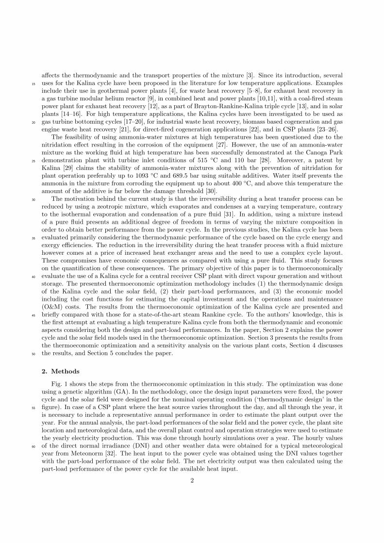
Fig. 1 shows the steps from the thermoeconomic optimization in this study. The optimization was doneusing a genetic algorithm (GA). In the methodology, once the design input parameters were fixed, the powercycle and the solar field were designed for the nominal operating condition (‘thermodynamic design’ in thefigure). In case of a CSP plant where the heat source varies throughout the day, and all through the year, it55

is necessary to include a representative annual performance in order to estimate the plant output over theyear. For the annual analysis, the part-load performances of the solar field and the power cycle, the plant sitelocation and meteorological data, and the overall plant control and operation strategies were used to estimatethe yearly electricity production. This was done through hourly simulations over a year. The hourly valuesof the direct normal irradiance (DNI) and other weather data were obtained for a typical meteorological60

year from Meteonorm [32]. The heat input to the power cycle was obtained using the DNI values togetherwith the part-load performance of the solar field. The net electricity output was then calculated using thepart-load performance of the power cycle for the available heat input.

2

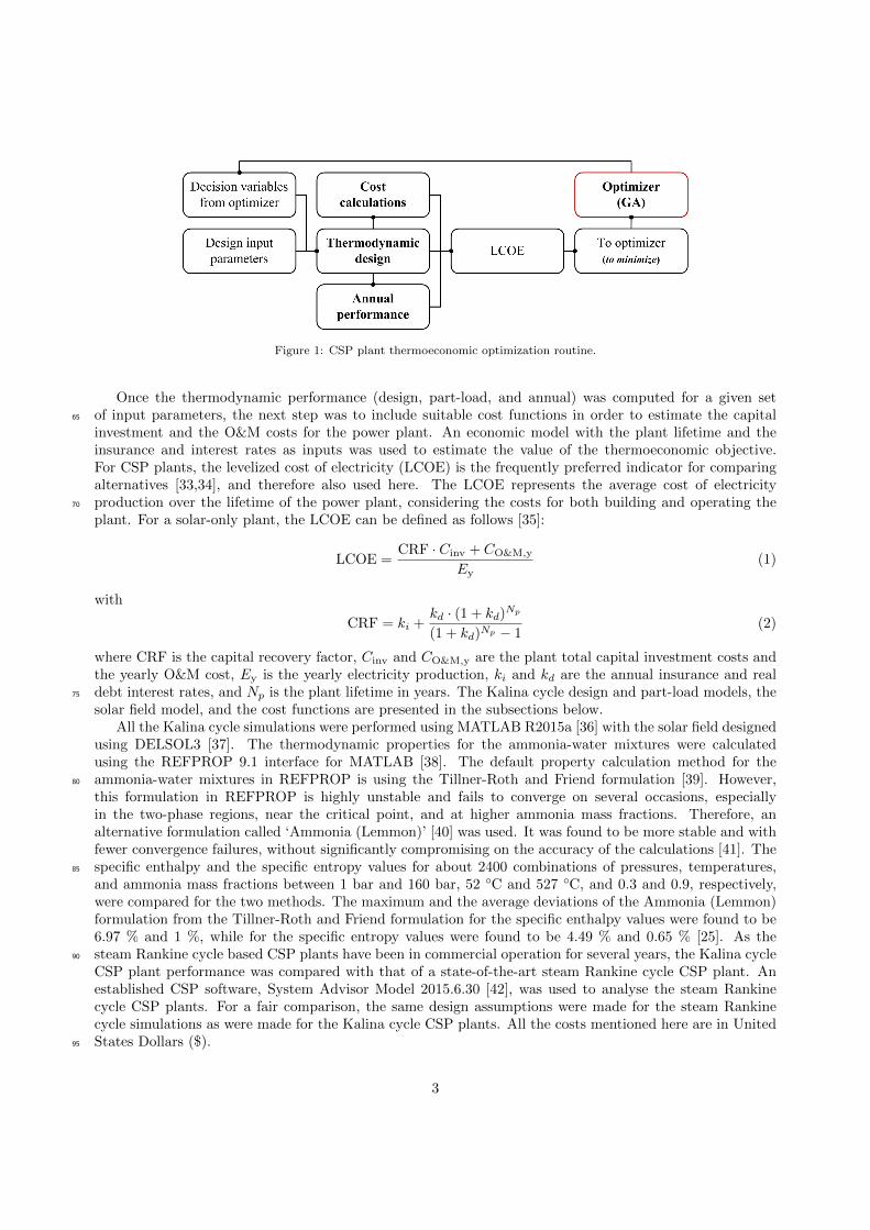
Figure 1: CSP plant thermoeconomic optimization routine.

Once the thermodynamic performance (design, part-load, and annual) was computed for a given setof input parameters, the next step was to include suitable cost functions in order to estimate the capital65

investment and the O&M costs for the power plant. An economic model with the plant lifetime and theinsurance and interest rates as inputs was used to estimate the value of the thermoeconomic objective.For CSP plants, the levelized cost of electricity (LCOE) is the frequently preferred indicator for comparingalternatives [33,34], and therefore also used here. The LCOE represents the average cost of electricityproduction over the lifetime of the power plant, considering the costs for both building and operating the70

plant. For a solar-only plant, the LCOE can be defined as follows [35]:

LCOE =CRF · Cinv + CO&M,y

Ey(1)

with

CRF = ki +kd · (1 + kd)Np

(1 + kd)Np − 1(2)

where CRF is the capital recovery factor, Cinv and CO&M,y are the plant total capital investment costs andthe yearly O&M cost, Ey is the yearly electricity production, ki and kd are the annual insurance and realdebt interest rates, and Np is the plant lifetime in years. The Kalina cycle design and part-load models, the75

solar field model, and the cost functions are presented in the subsections below.All the Kalina cycle simulations were performed using MATLAB R2015a [36] with the solar field designed

using DELSOL3 [37]. The thermodynamic properties for the ammonia-water mixtures were calculatedusing the REFPROP 9.1 interface for MATLAB [38]. The default property calculation method for theammonia-water mixtures in REFPROP is using the Tillner-Roth and Friend formulation [39]. However,80

this formulation in REFPROP is highly unstable and fails to converge on several occasions, especiallyin the two-phase regions, near the critical point, and at higher ammonia mass fractions. Therefore, analternative formulation called ‘Ammonia (Lemmon)’ [40] was used. It was found to be more stable and withfewer convergence failures, without significantly compromising on the accuracy of the calculations [41]. Thespecific enthalpy and the specific entropy values for about 2400 combinations of pressures, temperatures,85

and ammonia mass fractions between 1 bar and 160 bar, 52 ◦C and 527 ◦C, and 0.3 and 0.9, respectively,were compared for the two methods. The maximum and the average deviations of the Ammonia (Lemmon)formulation from the Tillner-Roth and Friend formulation for the specific enthalpy values were found to be6.97 % and 1 %, while for the specific entropy values were found to be 4.49 % and 0.65 % [25]. As thesteam Rankine cycle based CSP plants have been in commercial operation for several years, the Kalina cycle90

CSP plant performance was compared with that of a state-of-the-art steam Rankine cycle CSP plant. Anestablished CSP software, System Advisor Model 2015.6.30 [42], was used to analyse the steam Rankinecycle CSP plants. For a fair comparison, the same design assumptions were made for the steam Rankinecycle simulations as were made for the Kalina cycle CSP plants. All the costs mentioned here are in UnitedStates Dollars ($).95

3

2.1. Kalina cycle

The Kalina cycle layout investigated in this paper, named KC12 [25], is shown in Fig. 2. The cyclecomponents in the layout are shown in abbreviated forms where REC is the receiver/boiler, TUR is theturbine, GEN is the generator, SEP is the vapour-liquid separator, RE∗ is the recuperator, PU∗ is the pump,CD∗ is the condenser, MX∗ is the mixer (where ‘∗’ denotes the respective component number), SPL is the100

splitter, and THV is the throttling valve.

Figure 2: Kalina cycle KC12.

In the cycle, the superheated ammonia-water mixture (stream 1), i.e. the working solution, expands inthe turbine and is subsequently mixed in the mixer MX1 with the ammonia lean liquid from the separatorSEP to lower the ammonia mass fraction in the condenser CD1. The fluid after the mixer MX1 is called thebasic solution. The ammonia rich vapour from the separator SEP is mixed in the mixer MX2 with a part105

of the basic solution from the splitter SPL in order to obtain the working solution ammonia mass fraction.This working solution then passes through the condenser CD2 and the pump PU2. The external heat inputto the working fluid is provided in the solar receiver REC.

A methodology to obtain the nominal operating condition for the Kalina cycle KC12 was presented indetail by Modi et al. [26]. The validation of the general solution algorithm for the high temperature Kalina110

cycles was also presented [26]. The following assumptions were made for the thermodynamic design of theKalina cycle CSP plant [25,35]. The plant was designed for a net electrical power output (Wnet) of 20 MW.

4

Figure 3: Solution algorithm for the thermodynamic design of the Kalina cycle KC12.

The turbine inlet temperature (T1) was fixed at 500 ◦C. The design point isentropic efficiency was 85 %for the turbine (ηtur,is) and 70 % for the pumps (ηpu,is). The turbine mechanical efficiency (ηtur,m)and thegenerator efficiency (ηgen) were both 98 %. The minimum allowed vapour quality at the turbine outlet115

(X2,min) was 90 %. The condenser cooling water inlet (Tcw,in) and outlet (Tcw,out) temperatures were fixedat 20 ◦C and 30 ◦C, respectively. The recuperators (∆Tpp,re,min) and the condensers (∆Tpp,cd,min) had aminimum pinch point temperature difference of 8 ◦C and 4 ◦C, respectively. The minimum separator inletvapour quality (X10,min) was fixed at 5 %, and the pressure drops and heat losses were neglected. For theeconomic model, the plant lifetime (Np) was assumed to be 30 years and the annual insurance rate (ki) and120

the real debt interest rate (kd) were assumed to be 1 % and 8 %, respectively [35].For brevity, the methodology to obtain the nominal operating condition for the Kalina cycle KC12 is

presented as a flow chart in Fig. 3. In general, the following steps were used to solve the Kalina cycle foreach iteration of the optimization process [26]. The turbine TUR was solved first to obtain the state atthe turbine outlet. Assuming a condenser pressure for the condenser CD2, the mass flow rates were then125

obtained using a simplified configuration as presented in Marston [17] and elaborated in Modi et al. [26]for the KC12 layout. Once the mass flow rates at different points in the cycle were known, and it wasmade sure that the inlet stream to the separator SEP is in two-phase flow, then the pumps, the mixers,the recuperators, and the condensers were solved using the equations as presented in Modi et al. [26], whilesatisfying all the design constraints.130

In addition to the cycle thermodynamic design, the heat exchanger areas were also estimated in orderto assess the associated costs. The heat exchangers were modelled following the general approach presented

5

by Kærn et al. [43]. For large heat transfer capacities, it is common to use shell-and-tube type heatexchangers [44], therefore all the heat exchangers in this study were modelled as shell-and-tube type withcounter-flow arrangement. The heat exchangers were assumed to have a single shell pass and a single tube135

pass. The fluid with higher pressure was always put on the tube side as it is less expensive to have highpressure tubes than high pressure shells; and wherever possible, the two-phase flow would be put on the tubeside so as to avoid high variation in the mixture composition at different parts of the heat exchanger [45,46].In case there was a two-phase to two-phase heat transfer, the evaporating fluid was put on the tube sidewhile the condensing fluid was put on the shell side, mainly because the evaporating sides are usually the140

high pressure sides in the considered cycle layout (Fig. 2).The maximum flow velocities for the heat exchanger design were fixed based on the recommended values

by Nag [44] and Sinnott [46], in order to attain a reasonable compromise between the heat transfer andpressure drop based on industrial experience. The maximum shell and tube side liquid velocities were fixedat 0.8 m s−1 and 2 m s−1, respectively [46]. The maximum vapour velocity on both the shell and the tube145

sides was fixed at 22 m s−1 [44] for the low and intermediate pressure heat exchangers (recuperator RE2 andthe condensers CD1 and CD2). The same was fixed at 10 m s−1 [46] for the high pressure heat exchanger(recuperator RE1). The tube outside diameter was assumed to be 20 mm while the tube thickness wasassumed to be 1.6 mm for the low and intermediate pressure heat exchangers, and 2.6 mm for the highpressure heat exchangers, two of the common standard tube sizes [46]. The 45 degrees square pattern was150

assumed for the tube arrangement to maximize the heat transfer [46]. The tube pitch to tube outer diameterratio was maintained between 1.25 and 1.5, and a baffle cut of 25 % was fixed for the heat exchanger areacalculations, two common design assumptions for shell-and-tube heat exchangers [46]. Using the geometricalconstraints and the design mass flow rates, the required number of tubes was minimized until the maximumallowable flow velocity was reached on either the shell or the tube side. As the temperature profiles in the155

heat exchangers were not always linear, the heat exchangers were discretized into 50 control volumes on thebasis of the heat transfer rate for pinch calculation. The total area of the heat exchanger would then be thesum of the areas of all the control volumes. Table 1 provides an overview of the heat transfer correlationsused in this study.

Table 1: Heat transfer correlations used in the estimation of the heat exchanger area.

Description Correlation

Single phase in-tube flow Gnielinski (1976) [47]Condensing in-tube flow Shah (2013) with Silver-Bell-Ghaly (1972) correction for

mixtures [48,49]Evaporating in-tube flow Shah (1982) [50]

Single phase shell-side flow Kern (1950) as presented in Smith (2005) [45,51]Condensing shell-side flow Kern (1950) as presented in Smith (2005), with Silver-Bell-

Ghaly (1972) correction for mixtures [45,49,51]

Once the thermodynamic states, the different mass flow rates, and the heat exchanger areas were esti-160

mated from the cycle design, the part-load calculations were performed as elaborated in Modi et al. [26]. Forthe part-load operation, the following control strategy was used. A sliding pressure operation was assumedwhile maintaining the turbine inlet temperature at the design value. In order to obtain the highest part-loadperformance from the cycle, the separator inlet ammonia mass fraction was varied. In practice, it is easier tomeasure the temperatures and pressures in the cycle than to measure the ammonia mass fraction, especially165

when the mixture is in two-phase flow. Since the pressure at the pump PU1 outlet is governed by thecondenser CD2, the splitter SPL split fraction (i.e. the ratio of the mass flow rate of stream 9 to that ofstream 7 in Fig. 2) needs to be varied to obtain the required optimal separator inlet ammonia mass fraction.This split fraction can be varied by changing the splitter SPL valve position, and this position in turndetermines the separator inlet ammonia mass fraction. For a given value of the pump PU1 outlet pressure170

(which is also the separator SEP inlet pressure), there will be only one combination of the temperature and

6

the ammonia mass fraction at the separator SEP inlet which results in the highest part-load performance.Thus, the separator SEP inlet temperature can be monitored in order to specify the optimal splitter valveposition (and thus the optimal split fraction) for the different part-load operating conditions. The differentplant equipment were modelled in part load as follows. The turbine was modelled in part load using the175

Stodola’s ellipse law which relates the temperature, pressure, and mass flow rate at the turbine inlet, andthe pressure at the turbine outlet [52] through a turbine constant (ktur) as shown below:

ktur =m1 ·

√T1√

p21 − p2

2

(3)

while the off-design isentropic efficiency of the turbine was estimated from [53]:

ηtur,is = ηtur,is,d − 2 ·

[Ntur

Ntur,d·

√∆his,tur,d

∆his,tur− 1

]2

(4)

where ηtur,is and ηtur,is,d are the turbine isentropic efficiencies at part-load and design conditions, Ntur andNtur,d are the turbine rotational speeds at part-load and design conditions, and ∆his,tur and ∆his,tur,d are180

the isentropic specific enthalpy differences across the turbine at part-load and design conditions. The turbinespeed in a power plant is always maintained at the design value in order to maintain the frequency of thegenerated electricity at a constant value, and therefore the ratio of the speeds in Eq. 4 is taken as unity [53].Although the mechanical losses typically remain constant in absolute terms during part-load operation, themechanical efficiency of the turbine was assumed to stay the same as its design value for simplification.185

The off-design isentropic efficiency of the pumps was obtained from [54]:

ηpu,is = ηpu,is,d ·

[2 · mpu

mpu,d−(mpu

mpu,d

)2]

(5)

where ηpu,is and ηpu,is,d are pump efficiencies at part-load and design conditions, and mpu and mpu,d arethe mass flow rate through the pump at part-load and design conditions.

The off-design generator efficiency was obtained from [55]:

ηgen =ηgen,d · ζgen

ηgen,d · ζgen + (1− ηgen,d) ·[(1− Fcu) + Fcu · ζ2

gen

] (6)

where Fcu is the copper loss fraction (assumed 0.43 [55]), ηgen and ηgen,d are the generator efficiencies at190

part-load and design conditions, and ζgen is the generator load relative to the design value.The heat exchangers were again discretized in the part-load conditions to obtain the temperature profiles

so as to ensure that there were no pinch violations. The UA values in part load were obtained using thepower law as shown below [26]:

(UA)i = (UA)i,d ·(m

md

)0.8

(7)

where (UA)i and (UA)i,d are the UA values at part-load and design conditions for the ith control volume, U195

is the overall heat transfer coefficient, A is the heat transfer area based on the tube outside diameter, andm and md are the mass flow rates of the cold fluid at part-load and design conditions.

2.2. Solar field

A central receiver solar field includes a number of heliostats with two-axis tracking to follow the sunand concentrate the sunlight on a receiver placed on the top of a tower. For the current study, an external200

cylindrical receiver with direct vapour generation and a surrounding heliostat field were assumed [56]. Thecentral receiver solar field was designed with Seville, Spain as the plant location (37.25◦N, 5.54◦W). Thislocation was considered as there are already several CSP plants that have been built in the region, and are

7

currently in operation [57]. A design DNI value of 900 W m−2 and a solar multiple of 1.3 were assumed [34].Fig. 4 highlights the various losses between the energy in the incident DNI and the final heat absorbed by205

the heat transfer fluid in the receiver. For the direct vapour generation configuration in this study, thereceiver heat transfer fluid is the same as the power cycle working fluid.

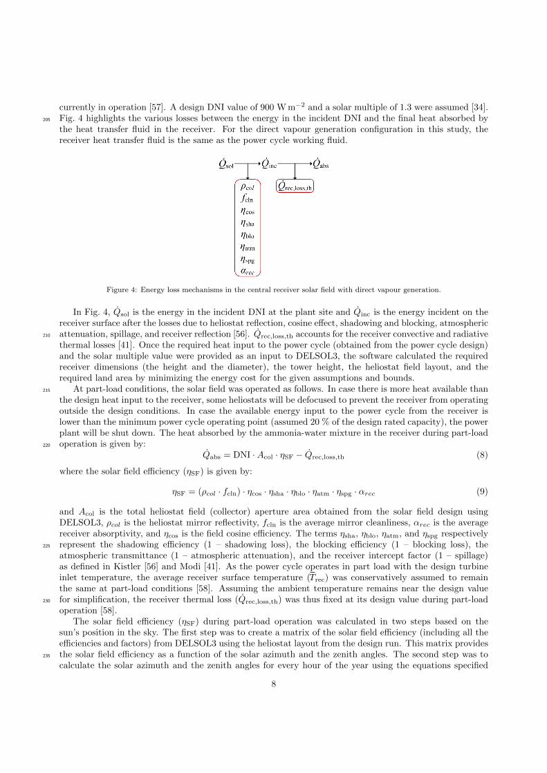
Figure 4: Energy loss mechanisms in the central receiver solar field with direct vapour generation.

In Fig. 4, Qsol is the energy in the incident DNI at the plant site and Qinc is the energy incident on thereceiver surface after the losses due to heliostat reflection, cosine effect, shadowing and blocking, atmosphericattenuation, spillage, and receiver reflection [56]. Qrec,loss,th accounts for the receiver convective and radiative210

thermal losses [41]. Once the required heat input to the power cycle (obtained from the power cycle design)and the solar multiple value were provided as an input to DELSOL3, the software calculated the requiredreceiver dimensions (the height and the diameter), the tower height, the heliostat field layout, and therequired land area by minimizing the energy cost for the given assumptions and bounds.

At part-load conditions, the solar field was operated as follows. In case there is more heat available than215

the design heat input to the receiver, some heliostats will be defocused to prevent the receiver from operatingoutside the design conditions. In case the available energy input to the power cycle from the receiver islower than the minimum power cycle operating point (assumed 20 % of the design rated capacity), the powerplant will be shut down. The heat absorbed by the ammonia-water mixture in the receiver during part-loadoperation is given by:220

Qabs = DNI ·Acol · ηSF − Qrec,loss,th (8)

where the solar field efficiency (ηSF) is given by:

ηSF = (ρcol · fcln) · ηcos · ηsha · ηblo · ηatm · ηspg · αrec (9)

and Acol is the total heliostat field (collector) aperture area obtained from the solar field design usingDELSOL3, ρcol is the heliostat mirror reflectivity, fcln is the average mirror cleanliness, αrec is the averagereceiver absorptivity, and ηcos is the field cosine efficiency. The terms ηsha, ηblo, ηatm, and ηspg respectivelyrepresent the shadowing efficiency (1 – shadowing loss), the blocking efficiency (1 – blocking loss), the225

atmospheric transmittance (1 – atmospheric attenuation), and the receiver intercept factor (1 – spillage)as defined in Kistler [56] and Modi [41]. As the power cycle operates in part load with the design turbineinlet temperature, the average receiver surface temperature (Trec) was conservatively assumed to remainthe same at part-load conditions [58]. Assuming the ambient temperature remains near the design valuefor simplification, the receiver thermal loss (Qrec,loss,th) was thus fixed at its design value during part-load230

operation [58].The solar field efficiency (ηSF) during part-load operation was calculated in two steps based on the

sun’s position in the sky. The first step was to create a matrix of the solar field efficiency (including all theefficiencies and factors) from DELSOL3 using the heliostat layout from the design run. This matrix providesthe solar field efficiency as a function of the solar azimuth and the zenith angles. The second step was to235

calculate the solar azimuth and the zenith angles for every hour of the year using the equations specified

8

in Duffie and Beckman [59], and interpolate the solar field efficiency for any hour from the matrix obtainedfrom DELSOL3. In this study, the solar angles were calculated at the beginning of every hour for their usein the annual performance calculations.

2.3. Cost functions240

The cost functions used to estimate the capital investment and the O&M costs are presented in thissection. In order to consider the effect of inflation since the cost functions were first published, all thecapital investment costs were scaled by the Marshall and Swift equipment cost indices to represent the costsin January 2014 values [60], except for the ones taken from NREL [42] as they were already from a 2015version of the software, and therefore maintained at the current values as a conservative assumption. The245

cost scaling was done by multiplying the cost obtained from the cost function by the equipment cost indexmultiplication factor, i.e. the ratio of the Marshall and Swift equipment cost index from January 2014, tothat of the year when the cost function was first published. An example is shown below:

C = CCF ·

(f2014

M&S

fCF,yM&S

)(10)

where C is the January 2014 cost, CCF is the cost estimated using the cost function, and f2014M&S and fCF,y

M&S

are the Marshall and Swift cost indices respectively for January 2014 and the year in which the cost function250

was first published. For brevity, all the capital cost functions are mentioned here without the equipmentcost index multiplication factor.

The total capital investment cost (Cinv) for the Kalina cycle CSP plant was estimated as the sum of thepower cycle cost (CPC), the solar field cost (CSF), the land purchasing cost (Cland), and the contingenciesover these three costs (Ccnt) as shown below:255

Cinv = CPC + CSF + Cland + Ccnt (11)

The power cycle cost was calculated using Eq. (12) as the sum of the equipment cost (CPC,eqp) and themiscellaneous cost (CPC,misc). The equipment cost (CPC,eqp) consisted of the capital investment cost forthe turbine (Ctur), the generator (Cgen), the pumps (Cpu), the heat exchangers – recuperators (Cre) andcondensers (Ccd), and the vapour-liquid separator (Csep), as shown in Eq. 13. The miscellaneous cost(CPC,misc) included the piping cost (CPC,pip), the instrumentation and control system cost (CPC,insc), theelectrical equipment and materials cost (CPC,el), and the installation cost (CPC,inst), as shown in Eq. 14.

CPC = CPC,eqp + CPC,misc (12)

CPC,eqp = Ctur + Cgen +∑

Cpu +∑

Cre +∑

Ccd + Csep (13)

CPC,misc = CPC,pip + CPC,insc + CPC,el + CPC,inst (14)

The Kalina cycle turbine and pump costs, with the turbine power output (Wtur) and the required pumppower (Wpu) in kW, were estimated using the correlations from Dorj [61]:

Ctur = 4405 · W 0.7tur (15)

Cpu = 1120 · W 0.7pu (16)

where the turbine power output (Wtur) and the required pump power (Wpu) were obtained as explained inModi et al. [26].

The cost of the generator and electrical auxiliaries were estimated using the generator electrical poweroutput (Wgen) in kW with the correlation by Pelster [62]:

Cgen = 10× 106 ·

(Wgen

160× 103

)0.7

(17)

9

The cost of the various heat exchangers in the cycle (the recuperators and the condensers) were estimated260

using the heat exchanger area (Ahx) with the correlation by Smith [45]:

Chx = 32 800 ·(Ahx

80

)0.8

· fpres · ftemp (18)

where the pressure (fpres) and the temperature (ftemp) correction factors were calculated as suggested inSmith [45].

The separator cost (Csep) was estimated assuming it to be a vertical vessel using the following equa-tion [63,64]:265

Csep = fpres · 10fs1+fs2·log10 Hsep+fs3·(log10 Hsep)2 (19)

where the height of the separator (Hsep) was calculated using the volumetric flow rate at the separatorinlet assuming a residence time of 3 min and a height to diameter ratio equal to 3, common specificationassumptions in commercial models [65]. The pressure correction factor (fpres) and the other cost factors(fs1, fs2, and fs3) were calculated as suggested in Ulrich [63]. The piping cost (CPC,pip), the instrumentationand control system cost (CPC,insc), the electrical equipment and material cost (CPC,el), and the installation270

cost (CPC,inst) were respectively assumed to be 66 %, 10 %, 10 %, and 45 % of the power cycle equipmentcosts (CPC,eqp) as suggested in Bejan et al. [66].

The total solar field cost (CSF) included the cost of the heliostat mirror collectors (Ccol), the tower(Ctow), the receiver (Crec), and site improvement (Csite) given by [42]:

CSF = Ccol + Ctow + Crec + Csite (20)

Ccol = 170 ·Acol (21)

Ctow = 3× 106 · exp

[0.0113 ·

(Htow −Hrec

2+Hcol

2

)](22)

Crec = 55 402 800 ·(π ·Drec ·Hrec

1110

)0.7

(23)

Csite = 15 ·Acol (24)

where Acol is the heliostat field total aperture area, Htow, Hrec, and Hcol are respectively the tower height,the receiver height, and the heliostat mirror height, and Drec is the receiver diameter.

The yearly O&M cost (CO&M,y) was the sum of the fixed and variable components. The yearly fixed275

O&M cost was $ 50 per kW of the plant rated capacity, while the variable O&M cost factor was $ 4 perMWh of the generated electricity [42]. The land purchasing cost (Cland) was assumed to be $ 10 000 peracre as suggested by NREL [42], where 1 acre is 4046.825 m2. The contingency cost (Ccnt) was assumed tobe 20 % of the sum of the solar field capital investment cost, the power cycle capital investment cost, andthe land purchase cost as suggested in the ECOSTAR report [35]:280

Ccnt = 0.2 · (CPC + CSF + Cland) (25)

A sensitivity analysis on the results of the thermoeconomic optimization was performed in order toidentify the parameters that affect the cost of the CSP plant the most. For the sensitivity analysis, thedifferent cost parameters for the Kalina cycle CSP plant were varied by ± 30 % from their optimal valuesand their effect on the LCOE was assessed. The varied parameters were the solar field capital investment cost(CSF), the power cycle capital investment cost (CPC), the land purchase cost (Cland), the contingency cost285

(Ccnt), and the fixed and variable O&M costs (CO&M,fix and CO&M,var). In addition, the capital investmentcost for the various solar field and power cycle components were also varied for a better insight into theresults.

10

3. Results

Fig. 5 shows the variation of the LCOE for different turbine inlet pressures and ammonia mass fractions290

at a turbine inlet temperature of 500 ◦C. The results suggest that the LCOE is relatively more sensitive tothe turbine inlet pressure than the turbine inlet ammonia mass fraction. All the combinations of the turbineinlet pressures and ammonia mass fractions result in a close range of LCOE values, between 212.2 $ MWh−1

and 218.9 $ MWh−1. This is because of the large share of the solar field in the capital investment cost(about 53 %) which governs the overall cost structure of the plant. The total plant specific investment cost295

(Cinv) for the different Kalina cycle cases is between 5322.7 $ kW−1 and 5559.8 $ kW−1. The values of thekey parameters from the thermoeconomic optimization are shown in Appendix A (Table A.1). For a similarcapacity plant, the state-of-the-art steam Rankine cycle had an LCOE of 181.0 $ MWh−1 with the plantspecific investment cost (Cinv) equal to 4822.3 $ kW−1.

Figure 5: Optimal LCOE values for the Kalina cycle central receiver CSP plant for various combinations of the turbine inletpressures and ammonia mass fractions.

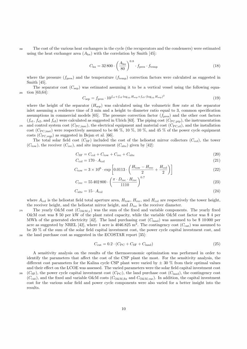
Among the various specific investment costs, the solar field specific investment cost (CSF) is directly300

related to the power cycle efficiency. A cycle with a lower efficiency requires a higher heat input for thesame net electrical power output. This required heat input then governs the solar field design, and as aresult the capital investment cost. This trend may be observed by comparing the respective power cycleefficiency (ηcy) and the solar field specific investment cost (CSF) values, and is shown in Fig. 6 for all thesimulated combinations of turbine inlet pressures and ammonia mass fractions.305

11

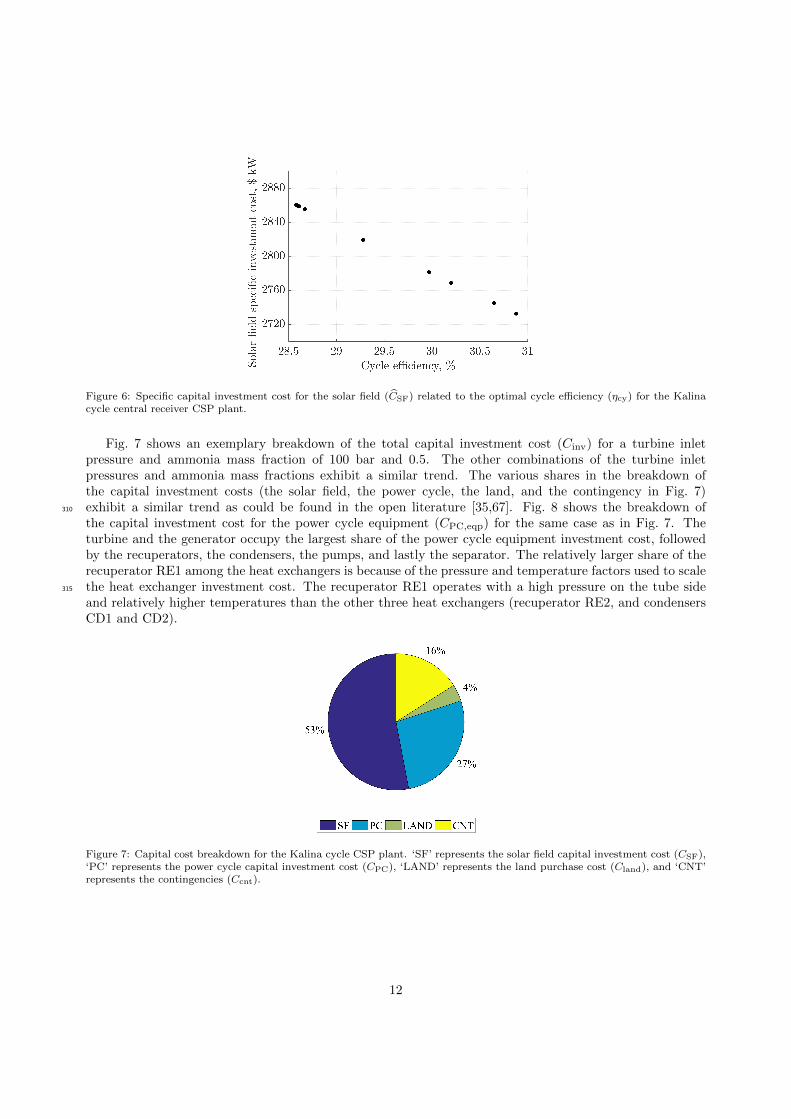
Figure 6: Specific capital investment cost for the solar field (CSF) related to the optimal cycle efficiency (ηcy) for the Kalinacycle central receiver CSP plant.

Fig. 7 shows an exemplary breakdown of the total capital investment cost (Cinv) for a turbine inletpressure and ammonia mass fraction of 100 bar and 0.5. The other combinations of the turbine inletpressures and ammonia mass fractions exhibit a similar trend. The various shares in the breakdown ofthe capital investment costs (the solar field, the power cycle, the land, and the contingency in Fig. 7)exhibit a similar trend as could be found in the open literature [35,67]. Fig. 8 shows the breakdown of310

the capital investment cost for the power cycle equipment (CPC,eqp) for the same case as in Fig. 7. Theturbine and the generator occupy the largest share of the power cycle equipment investment cost, followedby the recuperators, the condensers, the pumps, and lastly the separator. The relatively larger share of therecuperator RE1 among the heat exchangers is because of the pressure and temperature factors used to scalethe heat exchanger investment cost. The recuperator RE1 operates with a high pressure on the tube side315

and relatively higher temperatures than the other three heat exchangers (recuperator RE2, and condensersCD1 and CD2).

Figure 7: Capital cost breakdown for the Kalina cycle CSP plant. ‘SF’ represents the solar field capital investment cost (CSF),‘PC’ represents the power cycle capital investment cost (CPC), ‘LAND’ represents the land purchase cost (Cland), and ‘CNT’represents the contingencies (Ccnt).

12

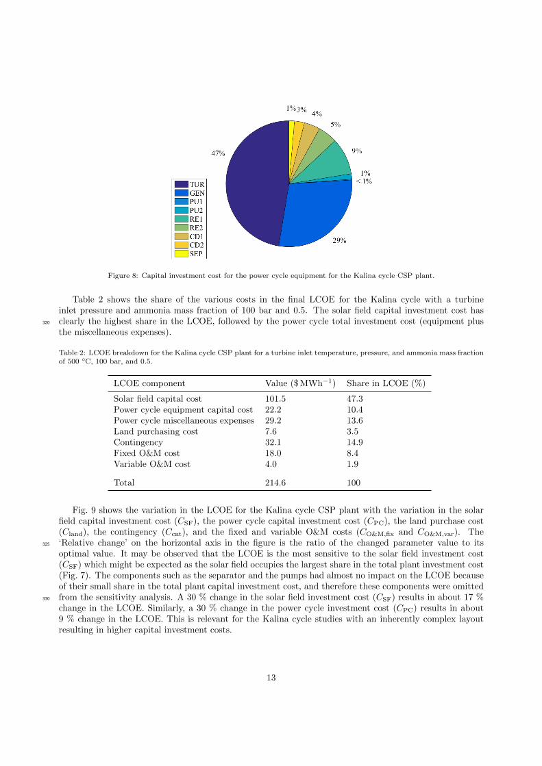
Figure 8: Capital investment cost for the power cycle equipment for the Kalina cycle CSP plant.

Table 2 shows the share of the various costs in the final LCOE for the Kalina cycle with a turbineinlet pressure and ammonia mass fraction of 100 bar and 0.5. The solar field capital investment cost hasclearly the highest share in the LCOE, followed by the power cycle total investment cost (equipment plus320

the miscellaneous expenses).

Table 2: LCOE breakdown for the Kalina cycle CSP plant for a turbine inlet temperature, pressure, and ammonia mass fractionof 500 ◦C, 100 bar, and 0.5.

LCOE component Value ($ MWh−1) Share in LCOE (%)

Solar field capital cost 101.5 47.3Power cycle equipment capital cost 22.2 10.4Power cycle miscellaneous expenses 29.2 13.6Land purchasing cost 7.6 3.5Contingency 32.1 14.9Fixed O&M cost 18.0 8.4Variable O&M cost 4.0 1.9

Total 214.6 100

Fig. 9 shows the variation in the LCOE for the Kalina cycle CSP plant with the variation in the solarfield capital investment cost (CSF), the power cycle capital investment cost (CPC), the land purchase cost(Cland), the contingency (Ccnt), and the fixed and variable O&M costs (CO&M,fix and CO&M,var). The‘Relative change’ on the horizontal axis in the figure is the ratio of the changed parameter value to its325

optimal value. It may be observed that the LCOE is the most sensitive to the solar field investment cost(CSF) which might be expected as the solar field occupies the largest share in the total plant investment cost(Fig. 7). The components such as the separator and the pumps had almost no impact on the LCOE becauseof their small share in the total plant capital investment cost, and therefore these components were omittedfrom the sensitivity analysis. A 30 % change in the solar field investment cost (CSF) results in about 17 %330

change in the LCOE. Similarly, a 30 % change in the power cycle investment cost (CPC) results in about9 % change in the LCOE. This is relevant for the Kalina cycle studies with an inherently complex layoutresulting in higher capital investment costs.

13

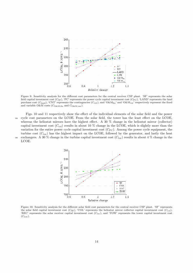
Figure 9: Sensitivity analysis for the different cost parameters for the central receiver CSP plant. ‘SF’ represents the solarfield capital investment cost (CSF), ‘PC’ represents the power cycle capital investment cost (CPC), ‘LAND’ represents the landpurchase cost (Cland), ‘CNT’ represents the contingencies (Ccnt), and ‘O&Mfix’ and ‘O&Mvar’ respectively represent the fixedand variable O&M costs (CO&M,fix and CO&M,var).

Figs. 10 and 11 respectively show the effect of the individual elements of the solar field and the powercycle cost parameters on the LCOE. From the solar field, the tower has the least effect on the LCOE,335

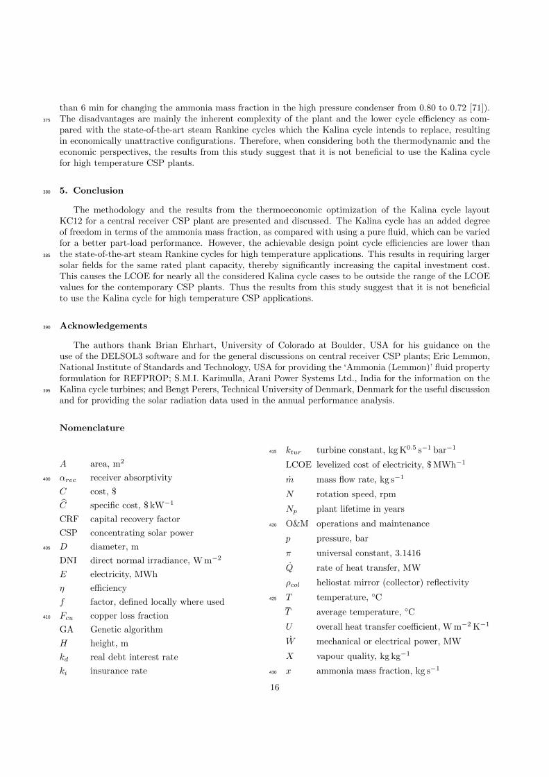
whereas the heliostat mirrors have the highest effect. A 30 % change in the heliostat mirror (collector)capital investment cost (Ccol) results in about 10 % change in the LCOE, which is slightly more than thevariation for the entire power cycle capital investment cost (CPC). Among the power cycle equipment, theturbine cost (Ctur) has the highest impact on the LCOE, followed by the generator, and lastly the heatexchangers. A 30 % change in the turbine capital investment cost (Ctur) results in about 4 % change in the340

LCOE.

Figure 10: Sensitivity analysis for the different solar field cost parameters for the central receiver CSP plant. ‘SF’ representsthe solar field capital investment cost (CSF), ‘COL’ represents the heliostat mirror collector capital investment cost (Ccol),‘REC’ represents the solar receiver capital investment cost (Crec), and ‘TOW’ represents the tower capital investment cost(Ctow).

14

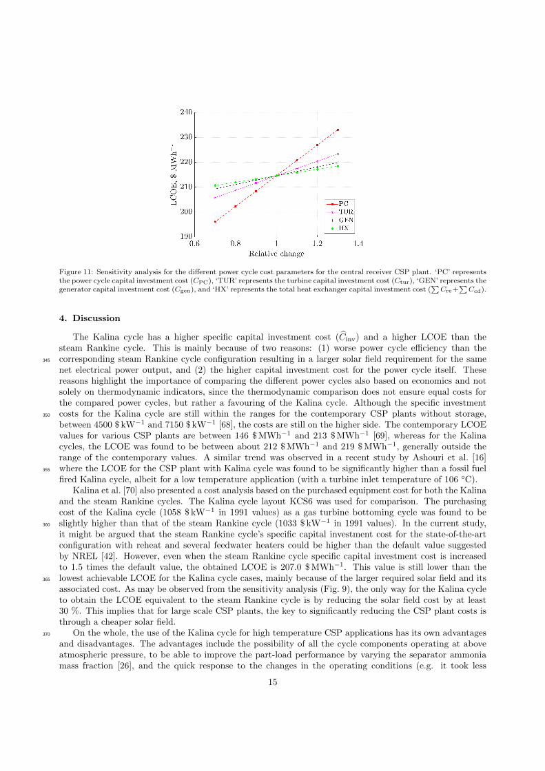
Figure 11: Sensitivity analysis for the different power cycle cost parameters for the central receiver CSP plant. ‘PC’ representsthe power cycle capital investment cost (CPC), ‘TUR’ represents the turbine capital investment cost (Ctur), ‘GEN’ represents thegenerator capital investment cost (Cgen), and ‘HX’ represents the total heat exchanger capital investment cost (

∑Cre+

∑Ccd).

4. Discussion

The Kalina cycle has a higher specific capital investment cost (Cinv) and a higher LCOE than thesteam Rankine cycle. This is mainly because of two reasons: (1) worse power cycle efficiency than thecorresponding steam Rankine cycle configuration resulting in a larger solar field requirement for the same345

net electrical power output, and (2) the higher capital investment cost for the power cycle itself. Thesereasons highlight the importance of comparing the different power cycles also based on economics and notsolely on thermodynamic indicators, since the thermodynamic comparison does not ensure equal costs forthe compared power cycles, but rather a favouring of the Kalina cycle. Although the specific investmentcosts for the Kalina cycle are still within the ranges for the contemporary CSP plants without storage,350

between 4500 $ kW−1 and 7150 $ kW−1 [68], the costs are still on the higher side. The contemporary LCOEvalues for various CSP plants are between 146 $ MWh−1 and 213 $ MWh−1 [69], whereas for the Kalinacycles, the LCOE was found to be between about 212 $ MWh−1 and 219 $ MWh−1, generally outside therange of the contemporary values. A similar trend was observed in a recent study by Ashouri et al. [16]where the LCOE for the CSP plant with Kalina cycle was found to be significantly higher than a fossil fuel355

fired Kalina cycle, albeit for a low temperature application (with a turbine inlet temperature of 106 ◦C).Kalina et al. [70] also presented a cost analysis based on the purchased equipment cost for both the Kalina

and the steam Rankine cycles. The Kalina cycle layout KCS6 was used for comparison. The purchasingcost of the Kalina cycle (1058 $ kW−1 in 1991 values) as a gas turbine bottoming cycle was found to beslightly higher than that of the steam Rankine cycle (1033 $ kW−1 in 1991 values). In the current study,360

it might be argued that the steam Rankine cycle’s specific capital investment cost for the state-of-the-artconfiguration with reheat and several feedwater heaters could be higher than the default value suggestedby NREL [42]. However, even when the steam Rankine cycle specific capital investment cost is increasedto 1.5 times the default value, the obtained LCOE is 207.0 $ MWh−1. This value is still lower than thelowest achievable LCOE for the Kalina cycle cases, mainly because of the larger required solar field and its365

associated cost. As may be observed from the sensitivity analysis (Fig. 9), the only way for the Kalina cycleto obtain the LCOE equivalent to the steam Rankine cycle is by reducing the solar field cost by at least30 %. This implies that for large scale CSP plants, the key to significantly reducing the CSP plant costs isthrough a cheaper solar field.

On the whole, the use of the Kalina cycle for high temperature CSP applications has its own advantages370

and disadvantages. The advantages include the possibility of all the cycle components operating at aboveatmospheric pressure, to be able to improve the part-load performance by varying the separator ammoniamass fraction [26], and the quick response to the changes in the operating conditions (e.g. it took less

15

than 6 min for changing the ammonia mass fraction in the high pressure condenser from 0.80 to 0.72 [71]).The disadvantages are mainly the inherent complexity of the plant and the lower cycle efficiency as com-375

pared with the state-of-the-art steam Rankine cycles which the Kalina cycle intends to replace, resultingin economically unattractive configurations. Therefore, when considering both the thermodynamic and theeconomic perspectives, the results from this study suggest that it is not beneficial to use the Kalina cyclefor high temperature CSP plants.

5. Conclusion380

The methodology and the results from the thermoeconomic optimization of the Kalina cycle layoutKC12 for a central receiver CSP plant are presented and discussed. The Kalina cycle has an added degreeof freedom in terms of the ammonia mass fraction, as compared with using a pure fluid, which can be variedfor a better part-load performance. However, the achievable design point cycle efficiencies are lower thanthe state-of-the-art steam Rankine cycles for high temperature applications. This results in requiring larger385

solar fields for the same rated plant capacity, thereby significantly increasing the capital investment cost.This causes the LCOE for nearly all the considered Kalina cycle cases to be outside the range of the LCOEvalues for the contemporary CSP plants. Thus the results from this study suggest that it is not beneficialto use the Kalina cycle for high temperature CSP applications.

Acknowledgements390

The authors thank Brian Ehrhart, University of Colorado at Boulder, USA for his guidance on theuse of the DELSOL3 software and for the general discussions on central receiver CSP plants; Eric Lemmon,National Institute of Standards and Technology, USA for providing the ‘Ammonia (Lemmon)’ fluid propertyformulation for REFPROP; S.M.I. Karimulla, Arani Power Systems Ltd., India for the information on theKalina cycle turbines; and Bengt Perers, Technical University of Denmark, Denmark for the useful discussion395

and for providing the solar radiation data used in the annual performance analysis.

Nomenclature

A area, m2

αrec receiver absorptivity400

C cost, $

C specific cost, $ kW−1

CRF capital recovery factor

CSP concentrating solar power

D diameter, m405

DNI direct normal irradiance, W m−2

E electricity, MWh

η efficiency

f factor, defined locally where used

Fcu copper loss fraction410

GA Genetic algorithm

H height, m

kd real debt interest rate

ki insurance rate

ktur turbine constant, kg K0.5 s−1 bar−1415

LCOE levelized cost of electricity, $ MWh−1

m mass flow rate, kg s−1

N rotation speed, rpm

Np plant lifetime in years

O&M operations and maintenance420

p pressure, bar

π universal constant, 3.1416

Q rate of heat transfer, MW

ρcol heliostat mirror (collector) reflectivity

T temperature, ◦C425

T average temperature, ◦C

U overall heat transfer coefficient, W m−2 K−1

W mechanical or electrical power, MW

X vapour quality, kg kg−1

x ammonia mass fraction, kg s−1430

16

ζ relative load

Subscripts and components

abs absorbed energy by receiver working fluid

atm atmospheric transmittance

blo blocking435

cd condenser

CF cost function

cln mirror cleanliness

cnt contingency

col heliostat mirror collector440

cos cosine effect

cw condenser cooling water

d design

el electrical equipment and material

eqp power cycle equipment445

fix fixed

gen generator

hx heat exchanger

inc energy available on the receiver surface be-fore receiver thermal loss450

insc instrumentation and control

inst installation

inv investment

is isentropic

land required land area455

loss loss

m mechanical

M&S Marshall and Swift equipment cost index

min minimum

misc power cycle miscellaneous cost460

mx mixer

net net electrical power output

PC power cycle

pip piping

pp pinch point465

pres pressure

pu pump

re recuperator

rec solar central receiver

sep separator470

SF solar field

sha shadowing

site plant site improvement

sol available solar energy

spg spillage475

spl splitter

temp temperature

th thermal

thv throttle valve

tow tower480

tur turbine

var variable

y yearly or annual

Appendix

Fig. A.1 shows the cycle nominal operating state for an exemplary thermoeconomically optimal solution485

for a turbine inlet temperature, pressure, and ammonia mass fraction of 500 ◦C, 100 bar, and 0.5. Themain results from the thermoeconomic optimization of the Kalina cycle central receiver CSP plant for allthe simulated combinations of the turbine inlet pressures and ammonia mass fractions at a turbine inlettemperature of 500 ◦C are shown in Table A.1.

17

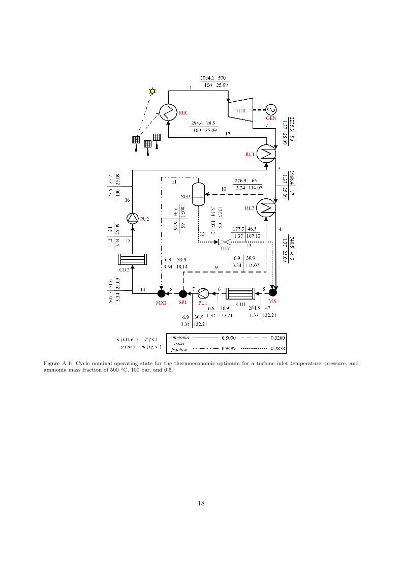
Figure A.1: Cycle nominal operating state for the thermoeconomic optimum for a turbine inlet temperature, pressure, andammonia mass fraction of 500 ◦C, 100 bar, and 0.5.

18

Table A.1: Thermoeconomic optimization results for the Kalina cycle central receiver CSP plant at a turbine inlet temperatureof 500 ◦C.

x1 p1 ηcy Cinv CSF CPC Cland Ccnt LCOE(bar) (%) ($ kW−1) ($ kW−1) ($ kW−1) ($ kW−1) ($ kW−1) ($ MWh−1)

0.5 100 28.58 5427.3 2860.8 1447.9 214.1 904.6 214.6120 28.67 5380.3 2855.5 1414.6 213.9 896.7 213.5140 28.58 5359.8 2860.8 1391.7 214.1 893.3 212.2

0.6 100 28.61 5559.8 2859.0 1560.3 213.9 926.6 218.9120 28.60 5482.2 2859.0 1495.6 213.9 913.7 216.2140 28.59 5428.7 2859.9 1450.1 214.0 904.8 214.2

0.7 100 28.58 5530.0 2860.8 1533.5 214.1 921.7 218.9120 29.28 5463.8 2819.3 1524.1 209.8 910.6 219.1140 30.20 5445.3 2768.9 1564.1 204.7 907.5 217.5

0.8 100 29.97 5432.3 2781.3 1539.7 206.0 905.4 218.8120 30.65 5372.6 2745.1 1529.7 202.4 895.4 216.0140 30.88 5322.7 2732.7 1501.7 201.2 887.1 214.1

References490

[1] Greenpeace International, SolarPACES, and ESTELA. Concentrating Solar Power: Global Outlook 2009. Technicalreport, Amsterdam, Netherlands, 2009.

[2] A.I. Kalina. Combined-cycle system with novel bottoming cycle. Journal of Engineering for Gas Turbines and Power,106:737–742, 1984.

[3] M.R. Kærn, A. Modi, J.K. Jensen, and F. Haglind. An assessment of transport property estimation methods for ammonia-495

water mixtures and their influence on heat exchanger size. International Journal of Thermophysics, 36(7):1468–1497, 2015.[4] A. Coskun, A. Bolatturk, and M. Kanoglu. Thermodynamic and economic analysis and optimization of power cycles for

a medium temperature geothermal resource. Energy Conversion and Management, 78:39–49, 2014.[5] P. Bombarda, C.M. Invernizzi, and C. Pietra. Heat recovery from diesel engines: A thermodynamic comparison between

Kalina and ORC cycles. Applied Thermal Engineering, 30(2-3):212–219, 2010.500

[6] H. Junye, C. Yaping, and W. Jiafeng. Thermal performance of a modified ammonia-water power cycle for reclaimingmid/low-grade waste heat. Energy Conversion and Management, 85:453–459, 2014.

[7] C. Yue, D. Han, W. Pu, and W. He. Comparative analysis of a bottoming transcritical ORC and a Kalina cycle for engineexhaust heat recovery. Energy Conversion and Management, 89:764–774, 2015.

[8] P. Zhao, J. Wang, and Y. Dai. Thermodynamic analysis of an integrated energy system based on compressed air energy505

storage (CAES) system and Kalina cycle. Energy Conversion and Management, 98:161–172, 2015.[9] V. Zare, S.M.S. Mahmoudi, and M. Yari. On the exergoeconomic assessment of employing Kalina cycle for GT-MHR

waste heat utilization. Energy Conversion and Management, 90:364–374, 2015.[10] S. Ogriseck. Integration of Kalina cycle in a combined heat and power plant, a case study. Applied Thermal Engineering,

29(14-15):2843–2848, 2009.510

[11] Z. Zhang, Z. Guo, Y. Chen, J. Wu, and J. Hua. Power generation and heating performances of integrated system ofammonia-water Kalina-Rankine cycle. Energy Conversion and Management, 92:517–522, 2015.

[12] O.K. Singh and S.C. Kaushik. Energy and exergy analysis and optimization of Kalina cycle coupled with a coal firedsteam power plant. Applied Thermal Engineering, 51(1-2):787–800, 2013.

[13] O.K. Singh and S.C. Kaushik. Thermoeconomic evaluation and optimization of a Brayton-Rankine-Kalina combined triple515

power cycle. Energy Conversion and Management, 71:32–42, 2013.[14] J. Wang, Z. Yan, E. Zhou, and Y. Dai. Parametric analysis and optimization of a Kalina cycle driven by solar energy.

Applied Thermal Engineering, 50(1):408–415, 2013.[15] F. Sun, W. Zhou, Y. Ikegami, K. Nakagami, and X. Su. Energy-exergy analysis and optimization of the solar-boosted

Kalina cycle system 11 (KCS-11). Renewable Energy, 66:268–279, 2014.520

[16] M. Ashouri, A.M. Khoshkar Vandani, M. Mehrpooya, M.H. Ahmadi, and A. Abdollahpour. Techno-economic assessmentof a Kalina cycle driven by a parabolic Trough solar collector. Energy Conversion and Management, 105:1328–1339, 2015.

[17] C.H. Marston. Parametric analysis of the Kalina cycle. Journal of Engineering for Gas Turbines and Power, 112:107–116,1990.

[18] C.H. Marston and M. Hyre. Gas turbine bottoming cycles: Triple-pressure steam versus Kalina. Journal of Engineering525

for Gas Turbines and Power, 117(January):10–15, 1995.

19

[19] M.B. Ibrahim and R.M. Kovach. A Kalina cycle application for power generation. Energy, 18(9):961–969, 1993.[20] P.K. Nag and A.V.S.S.K.S. Gupta. Exergy analysis of the Kalina cycle. Applied Thermal Engineering, 18(6):427–439,

1998.[21] E. Thorin. Power cycles with ammonia-water mixtures as working fluid. Phd thesis, KTH Royal Institute of Technology,530

Stockholm, Sweden, 2000.[22] C. Dejfors, E. Thorin, and G. Svedberg. Ammonia-water power cycles for direct-fired cogeneration applications. Energy

Conversion and Management, 39(16-18):1675–1681, 1998.[23] A. Modi, T. Knudsen, F. Haglind, and L.R. Clausen. Feasibility of using ammonia-water mixture in high temperature

concentrated solar power plants with direct vapour generation. Energy Procedia, 57:391–400, 2014.535

[24] A. Modi and F. Haglind. Performance analysis of a Kalina cycle for a central receiver solar thermal power plant withdirect steam generation. Applied Thermal Engineering, 65(1-2):201–208, 2014.

[25] A. Modi and F. Haglind. Thermodynamic optimisation and analysis of four Kalina cycle layouts for high temperatureapplications. Applied Thermal Engineering, 76:196–205, 2015.

[26] A. Modi, J.G. Andreasen, M.R. Kærn, and F. Haglind. Part-load performance of a high temperature Kalina cycle. Energy540

Conversion and Management, 105:453–461, 2015.[27] X. Zhang, M. He, and Y. Zhang. A review of research on the Kalina cycle. Renewable and Sustainable Energy Reviews,

16(7):5309–5318, 2012.[28] M.D. Mirolli. Kalina cycle power systems in waste heat recovery applications. www.globalcement.com/magazine/articles/

721-kalina-cycle-power-systems-in-waste-heat-recovery-applications. Accessed: 2015-07-08.545

[29] A.I. Kalina. Method of preventing nitridation or carburization of metals. United States Patent 6482272 B2, 2002.[30] Kalex LLC. Kalina cycle power systems for solar-thermal applications. www.kalexsystems.com/

KalexSolarThermalBrochure7-11.pdf. Accessed: 2015-06-13.[31] H. Chen, D.Y. Goswami, M.M. Rahman, and E.K. Stefanakos. A supercritical Rankine cycle using zeotropic mixture

working fluids for the conversion of low-grade heat into power. Energy, 36(1):549–555, 2011.550

[32] Meteotest. Meteonorm. www.meteonorm.com. Accessed: 2015-09-10.[33] C.-J. Winter, R.L. Sizmann, and L.L. Vant-Hull, editors. Solar power plants. Springer-Verlag, Heidelberg, Germany, 1st

edition, 1991.[34] K. Lovegrove and W. Stein, editors. Concentrating solar power technology: Principles, Developments and Applications.

Woodhead Publishing Limited, Cambridge, UK, 1st edition, 2012.555

[35] R. Pitz-Paal, J. Dersch, and B. Milow. ECOSTAR European Concentrated Solar Thermal Road-Mapping. Technicalreport, DLR, 2005.

[36] MathWorks. MATLAB. www.mathworks.se/products/matlab. Accessed: 2015-03-16.[37] Sandia National Laboratories. DELSOL. http://energy.sandia.gov/energy/renewable-energy/solar-energy/csp-2/

csp-codes-and-tools/. Accessed: 2015-06-24.560

[38] National Institute for Standards and Technology. REFPROP MATLAB Interface. www.boulder.nist.gov/div838/theory/refprop/LINKING/Linking.htm#MatLabApplications. Accessed: 2015-04-08.

[39] R. Tillner-Roth and D.G. Friend. A Helmholtz free energy formulation of the thermodynamic properties of the mixture{water+ammonia}. Journal of Physical and Chemical Reference Data, 27(1):63–96, 1998.

[40] E. Lemmon. National Institute of Standards and Technology. Private communication, 2013.565

[41] A. Modi. Numerical evaluation of the Kalina cycle for concentrating solar power plants. Phd thesis, Technical Universityof Denmark, Kongens Lngyby, Denmark, 2015.

[42] NREL. System Advisor Model. www.sam.nrel.gov. Accessed: 2015-06-25.[43] M.R. Kærn, A. Modi, J.K. Jensen, J.G. Andreasen, and F. Haglind. An assessment of in-tube flow boiling correlations

for ammonia-water mixtures and their influence on heat exchanger size. Applied Thermal Engineering, 93:623–638, 2016.570

[44] P.K. Nag. Power plant engineering. Tata Mc-Graw Hill Publishing Company Limited, New Delhi, India, 3rd edition,2008.

[45] R. Smith. Chemical Process - Design and Integration. John Wiley & Sons, Ltd., West Sussex, 2005.[46] R.K. Sinnott. Coulson & Richardson’s Chemical Engineering Volume 6. Elsevier Butterworth-Heinemann, Oxford, UK,

4th edition, 2005.575

[47] T.L. Bergman, A.S. Lavine, F.P. Incropera, and D.P. Dewitt. Fundamentals of heat and mass transfer. John Wiley &Sons, Inc., Jefferson City, USA, 7th edition, 2011.

[48] M.M. Shah, A.M. Mahmoud, and J. Lee. An assessment of some predictive methods for in-tube condensation heat transferof refrigerant mixtures. ASHRAE Transactions, 119(2):38–51, 2013.

[49] K.J. Bell and M.A. Ghaly. An approximate generalized design method for multicomponent/partial condensers. In 13th580

National Heat Transfer Conference, Denver, Colorado, USA, 1972. AIChE-ASME.[50] M.M. Shah. Chart correlation for saturated boiling heat transfer: equations and further study. ASHRAE Transactions,

88(1):185–196, 1982.[51] D.Q. Kern. Process Heat Transfer. McGraw-Hill Book Company, Singapore, 1950.[52] D.H. Cooke. Modeling of off-design multistage turbine pressures by Stodola’s ellipse. In Energy Incorporated PEPSE585

User’s Group Meeting, pages 205–234, Richmond, Virginia, USA, 1983. Bechtel Power Corporation.[53] A. Ray. Dynamic modelling of power plant turbines for controller design. Applied Mathematical Modelling, 4(2):109–112,

1980.[54] F. Lippke. Simulation of the part-load behavior of a 30 MWe SEGS plant. Technical report, Sandia National Laboratories,

SAND95-1293, 1995.590

[55] F. Haglind and B. Elmegaard. Methodologies for predicting the part-load performance of aero-derivative gas turbines.

20

Energy, 34(10):1484–1492, 2009.[56] B.L. Kistler. A user’s manual for DELSOL3: A computer code for calculating the optical performance and optimal system

design for solar thermal central receiver plants. Technical report, Sandia National Laboratories, Livermore, USA, 1986.[57] NREL. CSP projects. www.nrel.gov/csp/solarpaces/. Accessed: 2015-07-28.595

[58] B. Ehrhart. Univeristy of Colorado, Boulder. Private communication, 2015.[59] J.A. Duffie and W.A. Beckman. Solar Engineering of thermal processes. John Wiley & Sons, Inc., Hoboken, New Jersey,

USA, 4th edition, 2013.[60] Marshall Valuation Services. Comparative cost indexes, 2014.[61] P. Dorj. Thermoeconomic analysis of a new geothermal utilization CHP plant in Tsetserleg, Mongolia. Master thesis,600

The United Nations University, Reykjavik, Iceland, 2005.[62] S. Pelster. Environomic modelling and optimization of advanced combined cycle cogeneration power plants including CO2

separation options. Phd thesis, Ecole Polytechnique Federale de Lausanne, Lausanne, Switzerland, 1998.[63] G.D. Ulrich. A Guide to Chemical Engineering Process Design and Economics. John Wiley & Sons, Inc., New Jersey,

USA, 1984.605

[64] R. Turton, R.C. Bailie, W.B. Whiting, J.A. Shaeiwitz, and D. Bhattacharyya. Analysis, synthesis and design of chemicalprocesses. Prentice Hall, New Jersey, USA, 4th edition, 2012.

[65] The Alstrom Corporation. Two-phase flow separators. www.alstromcorp.com/PDFCatalogue/SECTION5/ALMUS.pdf. Ac-cessed: 2015-02-26.

[66] A. Bejan, G. Tsatsaronis, and M. Moran. Thermal Design & Optimization. John Wiley & Sons, Inc., 1st edition, 1996.610

[67] J.T. Hinkley, J.A. Hayward, B. Curtin, A. Wonhas, R. Boyd, C. Grima, A. Tadros, R. Hall, and K. Naicker. An analysisof the costs and opportunities for concentrating solar power in Australia. Renewable Energy, 57:653–661, 2013.

[68] IRENA. Renewable energy Technologies: Cost Analysis Series - Concentrating solar power. Technical report, InternationalRenewable Energy Agency, 2012.

[69] OECD and IEA. Technology roadmap - Solar thermal electricity. Technical report, International Energy Agency, Paris615

Cedex, France, 2014.[70] A.I. Kalina, H.M. Leibowitz, D.W. Markus, and R.I. Pelletier. Further technical aspects and economics of a utility-size

Kalina bottoming cycle. In Gas Turbine and Aeroengine Congress and Exposition, Orlando, Florida, USA, 1991. ASME.[71] C.H. Marston. Development of the adjustable proportion fluid mixture cycle. Mechanical Engineering, 114(9):76–81, 1992.

21