Thermodynamics of Restricted Boltzmann …Thermodynamics of Restricted Boltzmann Machines and...
40
Thermodynamics of Restricted Boltzmann Machines and Related Learning Dynamics Aur´ elien Decelle, Giancarlo Fissore, Cyril Furtlehner INRIA, LRI, Universit´ e Paris-Saclay TAU team
Transcript of Thermodynamics of Restricted Boltzmann …Thermodynamics of Restricted Boltzmann Machines and...

Thermodynamics of Restricted Boltzmann
Machines and Related Learning Dynamics
Aurelien Decelle, Giancarlo Fissore, Cyril Furtlehner
INRIA, LRI, Universite Paris-Saclay
TAU team
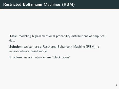
Restricted Boltzmann Machines (RBM)
Task: modeling high-dimensional probability distributions of empirical
data
Solution: we can use a Restricted Boltzmann Machine (RBM), a
neural-network based model
Problem: neural networks are ”black boxes”
1
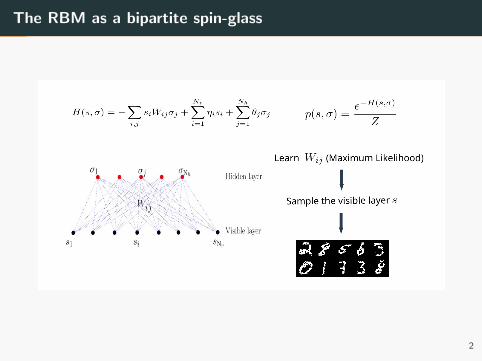
The RBM as a bipartite spin-glass
2

Linearized mean-field equations
Mean-field equation for the visible layer of the RBM:
mvi = sigm
ηi +∑
j
wijmhj −
∑j
wij
(mv = 〈s〉,mh = 〈σ〉
)Expanding over Singular Value Decomposition (SVD) components:
wij =∑α
wαui,αvj,α mvα =
∑i
ui,αmvi
⇓
mvα '
1
4wαm
hα
Magnetizations related to strong wα are amplified
3

Dynamics & statistical ensemble
• Dynamical evolution
dwαdt
= 〈sασα〉data − 〈sασα〉model , sα =∑
i
siui,α
• We need to define a statistical ensemble
wij =K∑α=1
wαui,αvj,α + rij
wα: singular values
ui,αvj,α: singular vectors components
rij : gaussian noise
Note: we average with respect to ui , vj and the noise rij keeping
sα, σα fixed.
4

Non-linear mean-field
• Thouless-Anderson-Palmer (TAP) free energy - ”numerical”
FTAP (mv ,mh) = + S(mv ) + S(mh)
−∑
i
ηimvi −
∑j
θjmhj −
∑i,j
wijmvi m
hj
+∑i,j
w2ij
2
(1−mv
i2)(
1−mhj
2)
• Replica symmetry framework - ”theoretical”
mvα =
(wαm
hα − ηα
)(1− qv
α)
mhα = (wαm
vα − θα)
(1− qh
α
)mvα = Eu,v ,r (〈sα〉) mh
α = Eu,v ,r (〈σα〉)qvα, q
hα: spin-glass order parameters 5
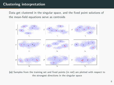
Clustering interpretation
Data get clustered in the singular space, and the fixed point solutions of
the mean-field equations serve as centroids
(a) Samples from the training set and fixed points (in red) are plotted with respect to
the strongest directions in the singular space
6
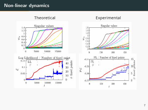
Non-linear dynamics
7
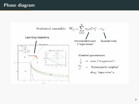
Phase diagram
8
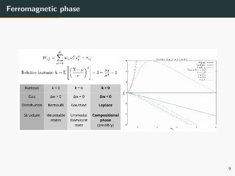
Ferromagnetic phase
9
Conclusion
Outcomes:
• comprehensive theoretical description of the model, both in linear
and non-linear regimes
• precise characterization of the learning dynamics (and definition of a
deterministic learning trajectory)
• assessment of the role and importance of the fixed point solutions of
the mean-field equations
• clustering interpretation of the training process
• characterization of the statistical properties of the weights of the
model
Perspectives:
• introducing symmetries: translational (and rotational) invariance
• dealing with lossy datasets
10

Thank you!
10

Overview of the RBM model

Definition of the model
RBM model: a neural network structured as a a bipartite graph
Specifically:
• a layer of hidden units hj and a layer of visible units vi are present
• data are represented as configurations of the visible layer
• there are not connections among units in the same layer
• we restrict our treatment to the case of binary units hi , vi = 0, 1
11

RBM training
• The probability of a visible configuration is given by
P(v) =∑
h
P(h, v) =e−Fc (v)
Z, Z =
∑v
e−Fc (v)
• We want to maximize P(v) for the samples belonging to the training
set
=⇒ gradient ascent over the log-likelihood logP(v)
Update rule
∆W = α(〈vhT 〉data − 〈vhT 〉model
)Problem: the term 〈·〉model is intractable
Best approximate algorithm: persistence contrastive divergence
(PCD), a Monte Carlo based method
12

The RBM and Statistical Physics
The RBM model is mapped to a Statistical Physics model by the
definition of an energy function
E (h, v) = −∑
i
aivi −∑
j
bjhj −∑i,j
viwijhj
P(h, v; W) =e−E(h,v)
Z
This let us borrow analytical and algorithmic tools from statistical
physics! In particular mean-field methods.
Remark: wij are the links connecting visible and hidden units and serve as
parameters of the model
13

Extended Mean Field (EMF) training
• The log-likelihood can be expressed as
logP(v) = loge−Fc (v)
Z= −
tractable︷ ︸︸ ︷Fc (v) − logZ︸ ︷︷ ︸
intractable
• F = logZ is the free energy of the system and it can be
approximated exploiting a high-temperature expansion1
New update rule
∆W = α
〈vhT 〉data −∂FTAP (mv , mh)
∂wij︸ ︷︷ ︸tractable
1A. Georges, J. S. Yedidia,
”How to expand around mean-field theory using high-temperature expansions”,
Journal of Physics A: Mathematical and General, Volume 24, Number 9, 1991.
14
EMF training
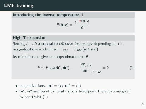
Introducing the inverse temperature β
P(h, v) =e−βE(h,v)
Z
High-T expansion
Setting β → 0 a tractable effective free energy depending on the
magnetizations is obtained: FTAP = FTAP (mv ,mh)
Its minimization gives an approximation to F :
F ' FTAP (mv , mh),dFTAP
dm
∣∣∣∣mv ,mh
= 0 (1)
• magnetizations: mv = 〈v〉,mh = 〈h〉• mv , mh are found by iterating to a fixed point the equations given
by constraint (1)
15
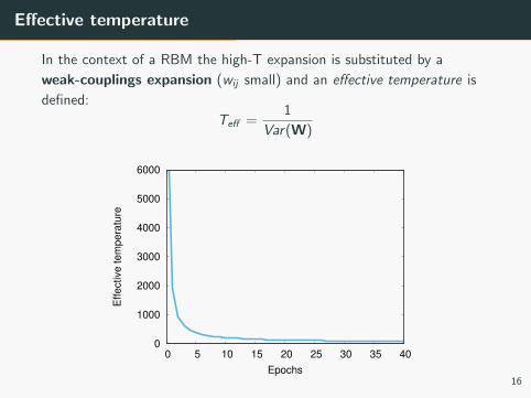
Effective temperature
In the context of a RBM the high-T expansion is substituted by a
weak-couplings expansion (wij small) and an effective temperature is
defined:
Teff =1
Var(W)
0
1000
2000
3000
4000
5000
6000
0 5 10 15 20 25 30 35 40
Effective tem
pera
ture
Epochs16

Comparison of PCD and EMF trainings
0
2
4
6
8
10
12
-0.6 -0.4 -0.2 0 0.2 0.4 0.6
Gaussian random matrix (σ = 0.01)
0
2
4
6
8
10
12
-0.6 -0.4 -0.2 0 0.2 0.4 0.6
PCD-5 - 50 epochs
0
2
4
6
8
10
12
-0.6 -0.4 -0.2 0 0.2 0.4 0.6
EMF - 50 epochs
(a) PCD features (b) EMF features
(c) MNIST
(d) PCD
(e) EMF
Learning dynamics are independent on the training procedure 17
Singular Value Decomposition (SVD)
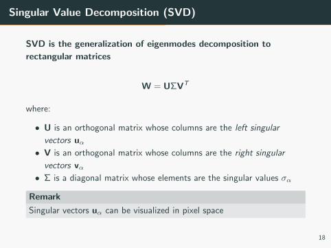
SVD is the generalization of eigenmodes decomposition to
rectangular matrices
W = UΣVT
where:
• U is an orthogonal matrix whose columns are the left singular
vectors uα• V is an orthogonal matrix whose columns are the right singular
vectors vα• Σ is a diagonal matrix whose elements are the singular values σα
Remark
Singular vectors uα can be visualized in pixel space
18
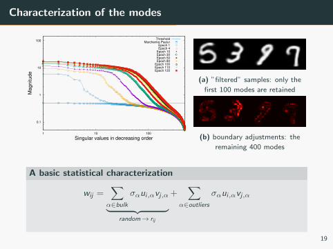
Characterization of the modes
0.1
1
10
100
1 10 100
Magnitude
Singular values in decreasing order
ThresholdMarchenko-Pastur
Epoch 1Epoch 4
Epoch 10Epoch 30Epoch 50Epoch 80
Epoch 100Epoch 110Epoch 120
(a) ”filtered” samples: only the
first 100 modes are retained
(b) boundary adjustments: the
remaining 400 modes
A basic statistical characterization
wij =∑α∈bulk
σαui,αvj,α︸ ︷︷ ︸random→ rij
+∑
α∈outliers
σαui,αvj,α
19
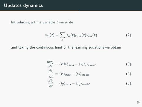
Updates dynamics
Introducing a time variable t we write
wij (t) =∑α
σα(t)µi,α(t)νj,α(t) (2)
and taking the continuous limit of the learning equations we obtain
dwij
dt= 〈vihj〉data − 〈vihj〉model (3)
dai
dt= 〈vi 〉data − 〈vi 〉model (4)
dbj
dt= 〈hj〉data − 〈hj〉model (5)
20
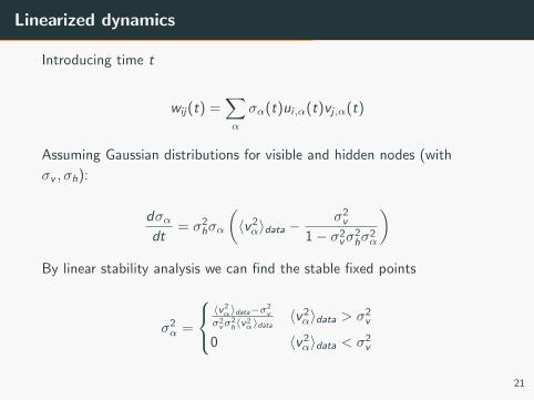
Linearized dynamics
Introducing time t
wij (t) =∑α
σα(t)ui,α(t)vj,α(t)
Assuming Gaussian distributions for visible and hidden nodes (with
σv , σh):
dσαdt
= σ2hσα
(〈v2α〉data −
σ2v
1− σ2vσ
2hσ
2α
)By linear stability analysis we can find the stable fixed points
σ2α =
〈v 2
α〉data−σ2v
σ2vσ
2h〈v 2
α〉data〈v2α〉data > σ2
v
0 〈v2α〉data < σ2
v
21
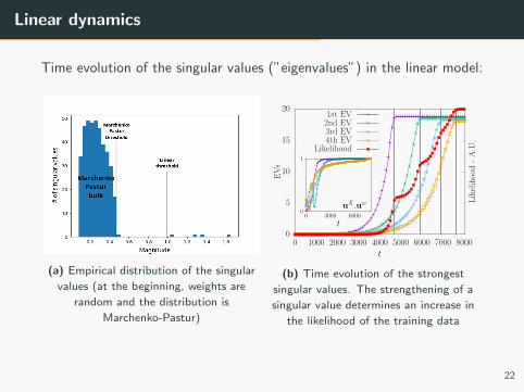
Linear dynamics
Time evolution of the singular values (”eigenvalues”) in the linear model:
(a) Empirical distribution of the singular
values (at the beginning, weights are
random and the distribution is
Marchenko-Pastur)
0
5
10
15
20
0 1000 2000 3000 4000 5000 6000 7000 8000
0
1
0 3000 6000uX.uw
EVs
Like
lihoo
d-A
.U.
t
1st EV2nd EV3rd EV4th EV
Likelihood
t
(b) Time evolution of the strongest
singular values. The strengthening of a
singular value determines an increase in
the likelihood of the training data
22
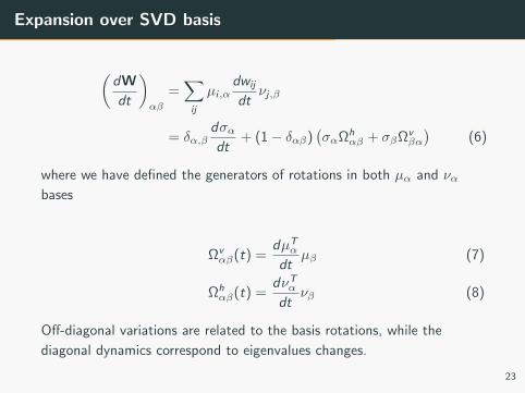
Expansion over SVD basis
(dW
dt
)αβ
=∑
ij
µi,αdwij
dtνj,β
= δα,βdσαdt
+ (1− δαβ)(σαΩh
αβ + σβΩvβα
)(6)
where we have defined the generators of rotations in both µα and ναbases
Ωvαβ(t) =
dµTα
dtµβ (7)
Ωhαβ(t) =
dνTα
dtνβ (8)
Off-diagonal variations are related to the basis rotations, while the
diagonal dynamics correspond to eigenvalues changes.
23

Update equations in SVD basis
Projecting the full learning equations on the SVD basis we obtain
(dW
dt
)αβ
= 〈vαhβ〉data − 〈vαhβ〉model (9)(da
dt
)α
= 〈vα〉data − 〈vα〉model (10)(db
dt
)α
= 〈hα〉data − 〈hα〉model (11)
with
vα =∑
i
viµi,α , hα =∑
j
hjνj,α (12)
24

Naive mean-field free energy
F (mv ,mh) =1
2
N∑i=1
(1 + mvi ) log(1 + mv
i ) + (1−mvi ) log(1−mv
i )
+1
2
M∑j=1
(1 + mhj ) log(1 + mh
j ) + (1−mhj ) log(1−mh
j )
−∑i,j
wijmvi m
hj +
N∑i=1
aimvi +
M∑j=1
bjmhj
' 1
2
N∑i=1
(mvi )2 +
1
2
M∑j=1
(mh
j
)2 −∑
ij
wijmvi m
hj
+N∑
i=1
aimvi +
M∑j=1
bjmhj (13)
25

Non-linear mean-field
• Thouless-Anderson-Palmer (TAP) free energy
FTAP (mv ,mh) = + S(mv ) + S(mh)
−∑
i
ηimvi −
∑j
θjmhj −
∑i,j
wijmvi m
hj
+∑i,j
w2ij
2
(1−mv
i2)(
1−mhj
2)
(14)
• Replica symmetry framework
mvα =
(σαm
hα − aα
)(1− qv
α)
mhα = (σαm
vα − bα)
(1− qh
α
)mvα = Eu,v ,r (〈vα〉) mh
α = Eu,v ,r (〈hα〉)
26

Gaussian approximation
cov(mv,mh) =
σ−2h
σ−2v σ−2
h −WWTW 1
σ−2v σ−2
h −WTW
WT 1σ−2
v σ−2h −WWT
σ−2h
σ−2v σ−2
h −WWT
(15)
⇓
〈vαhβ〉data = σ2hσβ〈vαvβ〉data = σ2
hσβ cov(vα, vβ) (16)
⇓
dσαdt
= σ2hσα
(〈v2α〉data −
σ2v
1− σ2vσ
2hσ
2α
)(17)
27
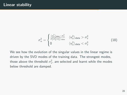
Linear stability
σ2α =
〈v 2
α〉data−σ2v
σ2vσ
2h〈v 2
α〉data〈v2α〉data > σ2
v
0 〈v2α〉data < σ2
v
(18)
We see how the evolution of the singular values in the linear regime is
driven by the SVD modes of the training data. The strongest modes,
those above the threshold σ2v , are selected and learnt while the modes
below threshold are damped.
28

Quenched mean-field equations
Statistical Physics kicks in! The Replica trick is used to get the
mean-field equations for the non-linear regime (in Replica Symmetry
setting)
mvα =
(σαm
hα − aα
)(1− qv
α)
mhα = (σαm
vα − bα)
(1− qh
α
)
mvα = Eu,v ,r (〈vα〉) mh
α = Eu,v ,r (〈hα〉)
where qvα, q
hα are spin-glass order parameters
Note: averages are taken with respect to ui , vj and the noise rij . The
specific realization of the weights is not important, just their distribution
is.
29
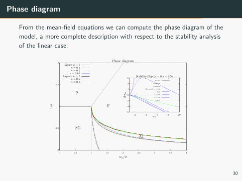
Phase diagram
From the mean-field equations we can compute the phase diagram of the
model, a more complete description with respect to the stability analysis
of the linear case:
0
0.5
1
1.5
2
0 0.5 1 1.5 2 2.5 3 3.5 4
1/σ
wα/σ
Phase diagram
F
P
SG
AT
-6
-4
-2
0
2
4
6
2 4 6 8 10
∆w
α
wα
Stability Gap (σ = 0 κ = 0.5)
Gauss κ = 1κ = 0.5κ = 0.1κ = 0.01
Laplace κ = 1κ = 0.5κ = 0.1
Gauss
Uniform
Laplace
Bernoulli r = 0.2
r = 1/3
r = 0.5
r = 0.9
r = 1
30
SVD analysis

Singular values evolution
Figure 10
31
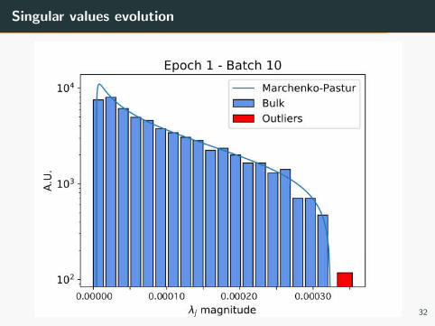
Singular values evolution
Figure 11
32

Singular values evolution
Figure 12
33
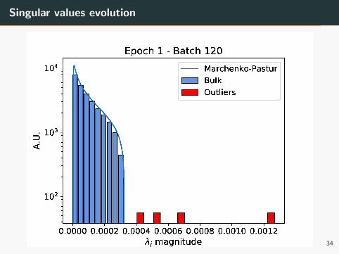
Singular values evolution
Figure 13
34
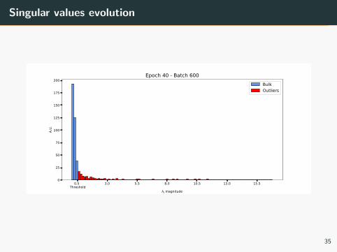
Singular values evolution
0.5 Threshold
3.0 5.5 8.0 10.5 13.0 15.5
λj magnitude
0
25
50
75
100
125
150
175
200
A.U.
Epoch 40 - Batch 600BulkOutliers
35

SVD modes
(a) SVD modes extracted from the training set
(b) The first 10 SVD modes of a RBM trained for 1 epoch
(c) Same as (b) but after a 10 epochs training
36


![Deep Restricted Boltzmann Networks - arXiv · learning. Restricted Boltzmann machine (RBM) [5] is one of such models that is simple but powerful. However, its restricted form also](https://static.fdocuments.in/doc/165x107/5ed27e2c773cd410be4fde3d/deep-restricted-boltzmann-networks-arxiv-learning-restricted-boltzmann-machine.jpg)