Te

Wa

b

a

ARAA

KIPMPE

1

icnif(maco

mmibebtrcsa

0d

Electrochimica Acta 56 (2010) 531–542

Contents lists available at ScienceDirect

Electrochimica Acta

journa l homepage: www.e lsev ier .com/ locate /e lec tac ta

hermodynamics and kinetics of phase transformation in intercalation batterylectrodes – phenomenological modeling

ei Laia,∗, Francesco Ciuccib

Department of Chemical Engineering and Materials Science, Michigan State University, East Lansing, MI 48824, USAHeidelberg Graduate School of Mathematical and Computational Methods for the Sciences, University of Heidelberg, INF 368 D – 69120 Heidelberg, Germany

r t i c l e i n f o

rticle history:eceived 3 September 2010ccepted 7 September 2010

a b s t r a c t

Thermodynamics and kinetics of phase transformation in intercalation battery electrodes are investigatedby phenomenological models which include a mean-field lattice-gas thermodynamic model and a gener-alized Poisson–Nernst–Planck equation set based on linear irreversible thermodynamics. The application

vailable online 21 September 2010

eywords:ntercalationhase transformationean-field lattice-gas model

of modeling to a porous intercalation electrode leads to a hierarchical equivalent circuit with elements ofexplicit physical meanings. The equivalent circuit corresponding to the intercalation particle of planar,cylindrical and spherical symmetry is reduced to a diffusion equation with concentration dependent dif-fusivity. The numerical analysis of the diffusion equation suggests the front propagation behavior duringphase transformation. The present treatment is also compared with the conventional moving boundary

es.

oisson–Nernst–Planckquivalent circuit

and phase field approach

. Introduction

Many battery electrodes undergo a phase transformation dur-ng the intercalation/insertion or deintercalation/extraction of thehemical species such as H, Li, Na etc. In the case of Li, this phe-omenon encompasses almost all the materials currently used

n commercial lithium ion batteries, such as three dimensionalramework compounds (LixMn2O4, LixTi5O12), layered compoundsLixCoO2, LixC6), and polyanion compounds (LixFePO4). In these

aterials, single or multiple phase transformation steps are actu-lly a universal phenomenon occurring for a wide range of Liomposition, x, while the formation of a solid solution is rare andnly exists for certain narrow ranges of x [1–8].

During phase transformation, a phase boundary develops andoves between coexisting phases. Two main approaches thatodel phase boundaries under phase transitions have emerged

n the literature. The first approach treats the phase boundaryetween two neighboring phases as a sharp interface and tracksxplicitly the movement of this interface. An example in lithiumattery electrode is the shrinking-core model [9]. In this model,he intercalation of Li species from the outer surface of the mate-

ial, which is taken to be a sphere, causes phase separation into aore–shell structure. Fick’s second law is used to describe the diffu-ion in the shell phase while the concentration in the core phase isssumed to be uniform. The movement of interface is determined

∗ Corresponding author. Tel.: +1 517 355 5126.E-mail address: laiwei@msu.edu (W. Lai).

013-4686/$ – see front matter © 2010 Elsevier Ltd. All rights reserved.oi:10.1016/j.electacta.2010.09.015

© 2010 Elsevier Ltd. All rights reserved.

by mass balance. This model was later extended to incorporate corediffusion by adding an additional equation to Fick’s second law [10].Recently, the mass balance at the interface was replaced by kineticequations, which consider the overpotential and mobility of theinterface [11]. In applied mathematics this moving boundary prob-lem is set up as two coupled partial differential equations and itis usually called Stefan’s problem [12]. Two common methods ofsolution are the Landau transformation that changes the movingboundary to a fixed boundary condition [10,13], and the movingmesh method [14,15].

The second approach, the phase field method, employs a phasefield variable to describe the smooth transition from one phase toanother and can be considered as a diffuse interface approach [16].In addition to its widespread application in solidification [17], thephase field method has recently been applied to the study of phasetransformation in battery electrodes [18–20]. It usually starts withCahn-Hilliard equation [21], which incorporates a concentrationgradient term to describe the interfacial energy and applies linearresponse theory to account for the driving force of the concentra-tion gradient.

The purpose of the present work is to develop a generalframework to study the phase transformation of intercalation bat-tery electrodes, on the basis of phenomenological thermodynamicmodels. The concept is that once a thermodynamic description

is established, the evolution of the system under the externalperturbation is completely determined by linear (assuming asmall driving force) irreversible thermodynamics. In Section 2,“Thermodynamics”, a simple lattice-gas model with mean-fieldapproximation is chosen to describe the thermodynamics of both

532 W. Lai, F. Ciucci / Electrochimica

Nomenclature

b mobilityc concentrationCchem chemical capacitanceCdis displacement/dielectric capacitanceD diffusivityD̃ chemical diffusivityF volumetric energyg interaction parameter in a lattice-gas modelI currentJm molar fluxj dimensionless current densityJ current densitym order of symmetryq volumetric charge densityr characteristic length along the planar, cylindrical

and spherical symmetryR resistancev velocityx dimensionless lengthX fraction of occupied sites in a latticez number of charges

Greek lettersεr relative permittivity� electrical potential� chemical potential�* reduced chemical potential�̃ electrochemical potential�̃∗ reduced electrochemical potential� geometrical factor

s“uPkcpmtdpat

2

wwltdmiaIwmi

� conductivity� dimensionless time

olid solution and phase transformation materials. In Section 3,Linear Irreversible Thermodynamics”, phenomenological modelsnder the driving force of electrochemical potential, generalizedoisson–Nernst–Planck (PNP) equations, is used to describe theinetics. It was found that PNP equations of a composite electrodean be mapped to a hierarchical equivalent circuit with explicithysical meanings. In Section 4, the application of lattice-gas ther-odynamic model of Section 2 to PNP equations of Section 3 lead

o a concentration dependent diffusion equation in the solid. Thisiffusion equation generates the front propagation behavior duringhase transformation. A qualitative comparison among the presentpproach, the moving boundary and phase field method is madehroughout the discussion.

. Thermodynamics

In this work, a lithium intercalation battery electrode particleill be taken as the example even though the general frame-ork described applies to other intercalation systems. When a

ithium ion (+) intercalates into a crystal structure, it can onlyake certain energetically favorable interstitial sites, e.g. tetrahe-ral, octahedral etc., while an electron (−) will go to the transitionetal ion as a large or small polaron. On the basis of this phys-

cal intuition a lattice-gas model with site exclusion seems to be

ppropriate to describe the thermodynamics of the lithium ion.n the present work, a simple statistical thermodynamic model

ith Bragg-Williams approximation [22] and mean-field approxi-ation [23], also called regular-solution model [19,21], is used for

llustration. This model is also named as Frumkin isotherm model

Acta 56 (2010) 531–542

[23–25] because the intercalation is a process in many ways similarto adsorption of atoms on a surface lattice. The description of thismodel is well documented in the literature so no derivation willbe given in this work. In this model, the volumetric free energy isgiven as [23]

F(X) = F0c0X + kBTc0 [X ln X + (1 − X) ln (1 − X)]

+ 12

kBTc0gX2, X = c

c0(1)

where F0 is the site energy, X is the fraction of occupied site con-centration c with respect to the total number of available sites c0,and g is the mean-field interaction parameter. kB is the Boltzmannconstant and T is the absolute temperature. The first term in (1) isthe internal energy, the second is the entropic term of mixing andthe third is the mean-field interaction term. gkBT represents theinteraction energy of an occupied site with its surroundings. Theinteraction is repulsive when g is positive and it is attractive inter-action when g is negative. The derivative of free energy with respectof the concentration gives the chemical potential. Specifically, forlithium ion, �+ is written as

�+ = �0+ + kBT ln

X

1 − X+ kBTg (X − 0.5) , X = c+

c0+(2)

where �0+ is the standard chemical potential. The second term in (2)is the entropic term featuring site exclusion (Fermi-Dirac statistics).The third term is anti-symmetrical about X = 0.5. When the inter-action parameter g is 0, it is reduced to the Langmuir isotherm andwhen X is small, it further reduces to the ideal-solution model. Itis noted that usually the concentration is written as a function ofchemical potential in isotherm model. In the regular solution model[19,21], the free energy is taking a different form as

F(X) = F1c0X + F2c0 (1 − X) + kBTc0 [X ln X + (1 − X) ln (1 − X)]

− 1/2kBTc0gX (1 − X) (3)

where F1 and F2 are the site energies of occupied and empty sitesrespectively. kBTg represents the interaction energy that includesoccupied versus occupied sites, empty versus empty sites and occu-pied versus empty sites. This energy form gives the same result forchemical potential as in equation (2).

The mathematical treatment of the intercalation electron ismore complicated because it depends on whether the electron islocalized and delocalized and on what the interaction terms are.The study of the electronic structure is generally necessary to pro-vide a complete picture of the chemical potential of the electron.For simplicity, the chemical potential of electron is assumed to beindependent of concentration in this work.

While the chemical potential is the derivative of the free energywith respect of the concentration, the derivative of chemical poten-tial with respect of concentration generates the thermodynamicfactor. The inverse of thermodynamic factor is physically moreinteresting since it is closely related to the concept of charge stor-age. In analogy to dielectric capacitance, a volumetric chemicalcapacitance term is introduced to reflect the change of charge uponthe change of chemical potential [26–28]

Cchemi = ∂qi

∂�∗i

= zie∂ci

∂�∗i

(4)

where zi is the number of charges per carrier, e is the electron charge

and qi is the volumetric charge density as zieci. �∗

i is called “reducedchemical potential” and has the unit of voltage as

�∗i = �i

zie(5)

W. Lai, F. Ciucci / Electrochimica

Fiap

a

C

1

23

aettrtcrcstsptcttL

ig. 1. (a) Dimensionless thermodynamic properties, chemical potential and chem-cal capacitance, and (b) dimensionless kinetic properties, chemical diffusivity, asfunction of concentration X. Different curves correspond to different interactionarameter of g explained in the text.

For the above simple lattice-gas model with lithium ion, Eqs. (2)nd (4) give

chem+ = e2c0+

kBT

[1

X (1 − X)+ g

]−1(6)

It is informative to plot the following dimensionless terms

. The chemical potential ln[X/(1 − X)

]+ g(X − 0.5) of (2),

. The chemical capacitance[1/(X(1 − X)) + g

]−1in (6),

. The chemical diffusivity 1 + gX(1 − X), see also (45).

s a function of X in Fig. 1 for three characteristic interaction param-ters of 0, −4, and −6. These three numbers are chosen to representhe solid solution, transition point between solid solution and phaseransition, and phase transformation with spinodal decompositionespectively. The two thermodynamic properties, chemical poten-ial and capacitance are shown in Fig. 1(a). It can be seen that thehemical potential has a monotonous dependence on X where g = 0,epresenting the solid solution behavior. When g = −6, the chemi-al potential exhibits spinodal decomposition behavior, where thepinodal points are those with local minimum or maximum inhe plot of chemical potential and are characterized by vanishingecond derivative of the free energy. When g = −4, the chemicalotential shows a “plateau” for the intermediate range of X. From

he viewpoint of thermodynamics, the chemical potential of Li inoexisting phases during a phase transformation is fixed; fromhe viewpoint of electrochemistry, the constant chemical poten-ial will lead to constant voltage versus the reference electrode, e.g.i/Li+, which exhibits as plateau in the voltage-composition plot.

Acta 56 (2010) 531–542 533

The kinetic property, chemical diffusivity, is shown in Fig. 1(b). Thechemical diffusivity shows no dependence on X when g = 0. This isthe usual case with constant chemical coefficient. Both g = −4 andg = −6 show concentration dependent diffusivity with a minimumat X = 0.5, with the minimum being 0 and −1/2 respectively.

For the electron, since the chemical potential is assumed to be aconstant, the chemical capacitance is infinite. Alternatively, underthe approximation of electroneutrality that will be shown later, itis useful to compare between the chemical capacitance due to theion (+) and the electron (−).

Cchem+Cchem−

= ∂c+∂�∗+

∂�∗−∂c−

= ∂�∗−∂�∗+

(7)

Here the electroneutrality condition reads c+ = c−. If it is assumedthat the change of electron chemical potential is much smaller thanthe change of ion chemical potential, then

Cchem+Cchem−

≈ 0 (8)

In either case, the chemical capacitance of lithium ion is muchsmaller than that of electron. This last expression is a key step inthe present derivation.

It is worth commenting on the limitations of (2) at this stageof the paper. Equation (2) corresponds to filling one regular latticeunder the assumption of mean-field. This mean-field approach isequivalent to considering only nearest neighbor interactions. Thesimple lattice-gas model can be easily extended to filling multi-ple sites and considering also second, third nearest neighbors byMonte Carlo simulation [29–35]. However, it was shown that themean-field approximation and Monte Carlo simulation give similarthermodynamic results [31]. Furthermore, strain accommodationenergy of different forms can be added to the expression of the freeenergy [11,20]. It is also worth comparing equations (1) or (2) withthe form used in the phase field. In the phase field method, the freeenergy term is equation (1) plus an interfacial energy term, whichis proportional the square of concentration gradient ( ∇ c)2 as inCahn-Hilliard equation [21]. This specific form is used to accountfor the thermodynamics of nonuniform systems. Mathematically,it can be considered as a Taylor expansion of free energy aroundequation (1), for a perturbation of concentration gradient ∇c. Thecoefficient of first order expansion vanishes due to symmetry [21].In other words, equation (1) and Cahn-Hilliard free energy termcan be considered as zero order and second order expansions for aperturbation of ∇c. Nonetheless, the special case g = −4 in the formof equation (2) is the focus of the current work and it will be shownthat the effective diffusivity has an analytical expression, whichexemplifies the situation of phase transition.

3. Linear irreversible thermodynamics

3.1. Generalized Poisson–Nernst–Planck equation set

Once the thermodynamic description of the system is estab-lished, understanding how the system will evolve under theexternal chemical, electrical, mechanical or coupled perturbation,is of primary theoretical and practical interest. In the present studylinear irreversible thermodynamics will be used. While mobile car-riers typically are treated as neutral species in the literature, herethey are taken to be charged and are considered to be movingunder electrochemical potentials as driving forces. The correla-

tion between the two treatments, neutral species under chemicalpotential versus charge carriers under electrochemical potentialwill be shown in later sections of this paper.

When the driving force is an electrochemical potential, theresult of linear irreversible thermodynamics is the generalized

5 himica

Pi(bbii[idh

cimtii

J

wtp

�

∇scmiei

a

�

J

w

�

t

z

C

−

wtowtwps

34 W. Lai, F. Ciucci / Electroc

oisson–Nernst–Planck (PNP) equation set. This equation setncludes Poisson equation (electrostatics), Nernst–Planck equationflux equation) and continuity equation and it is the theoreticalasis for modeling semiconductor devices [36], biological mem-ranes [37], electrochemistry [38] etc. The Nernst–Planck equation

s also called drift-diffusion in the field of semiconductors [36] andt is known as the diffusion-migration equation in electrochemistry38,39]. The complete description of PNP equation set can be foundn many literature references, with or without the assumption ofilute solution [26,27,40–42]. A brief discussion is still includedere for completeness.

By definition, molar flux of species i, Jmi , is the product of its

oncentration ci and its velocity vi. Under the theory of linearrreversible thermodynamics [43], the velocity is the product of

obility bi and the driving force. In the case of charge carriers,he driving force is the gradient of electrochemical potential �̃i,f convection and Onsager’s cross coefficients are ignored [39,43],.e.

mi = civi = −cibi∇�̃i (9)

here the electrochemical potential is the sum of chemical poten-ial �i and electrical energy zie�, in which � is the electricalotential.

˜ i = �i + zie� (10)

Just as the free energy can be considered as an expansion overc in the above discussion, the flux can be considered as an expan-

ion over the driving force ∇�̃i around zero flux (the equilibriumondition). The second order coefficient vanishes due to the sym-etry (the flux will change sign when the direction of driving force

s switched) so third order terms have to be used in order to correctquation (9). In the present work, only the first order term (linearrreversible thermodynamics) is used.

By introducing parameters such as current density, Ji = zieJmi

nd “reduced electrochemical potential”

˜ ∗i = �̃i

zie(11)

equation (9) can be written as

i = −�i∇�̃∗i = −�i∇�∗

i − �i∇� (12)

ith conductivity given by

i = (zie)2cibi = (zie)ci(ziebi) (13)

The reduced electrochemical �̃∗i

and chemical potential �∗i

havehe unit of voltages and ziebi is the definition electrical mobility.

Continuity equation reads

ie∂ci

∂t+ ∇ · J i = 0 (14)

With (4), the continuity equation can be written as

chemi

∂�∗i

∂t+ ∇ · J i = 0 (15)

The Poisson equation is

εrε0� =∑

i

zieci (16)

here εr and ε0 are the relative and vacuum permittivity and ishe Laplacian. εr is taken to be constant so a mechanistic discussionn the dielectric polarization is not made. The Poisson equation

ith the second spatial derivative, along with the continuity equa-

ion, can be transformed to a set of two equations in the sameay as in reference [26,27,41]. The first equation describes the dis-lacement current density Jdis. The second equation states that theum of all faradaic current densities and the non-faradaic current

Acta 56 (2010) 531–542

density (displacement current density) is the total current densityJT.

Then the generalized Poisson–Nernst–Planck equations havethe form of

J i = −�i∇�̃∗i

Cchemi

∂�∗i

∂t+ ∇ · J i = 0

Jdis = −εrε0∂

∂t(∇�)

JT = Jdis +∑

i

J i

(17)

The advantage of this formulation is that voltage and currentdensity terms are used instead of concentration terms. Thus, it isbe easier to construct equivalent circuits as shown later. However,for the purpose of comparison, it is still worthwhile to look at theflux equation in the form of concentration gradients. Converting thecurrent density back to the molar flux and utilizing the chemicaldiffusivity, (12) or the first equation in (17) becomes

Jmi = −D̃i∇ci − �i

zie∇� (18)

Here the definition of chemical diffusivity is

D̃i = �i

Cchemi

(19)

In the latter the chemical capacitance is a thermodynamicproperty while the conductivity is a kinetic property. Hence, thechemical diffusivity is also a kinetic property. In the phase fieldmethod, there is usually no accounting for the electron and dielec-tric flux, and the application of continuity equation will lead tofourth order differential equations depending solely on concentra-tions. This makes the numerical computations quite difficult.

3.2. Equivalent circuit for a two carrier system under symmetry

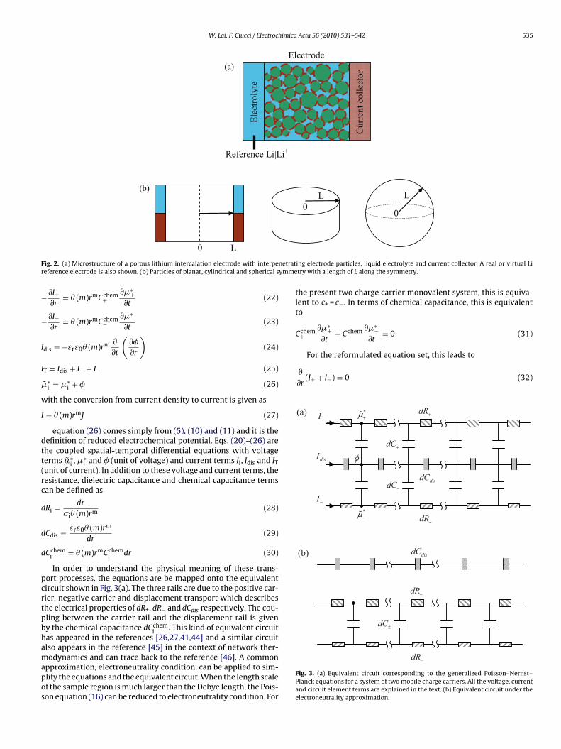
Even though what follows is applicable to many intercalationmaterials or systems, a porous lithium intercalation electrode willbe chosen as an example. The microstructure of the electrodeis shown in Fig. 2(a). It is a porous network of particles withinterpenetrating liquid electrolyte. The dashed circle around theparticle represents the interconnected yet porous current collectornetwork. The porous electrode is connected to a real or virtual refer-ence electrode, e.g. Li foil. Although shown as spherical in Fig. 2(a),particles of different symmetry are shown in Fig. 2(b) with a lengthof L along the symmetry. The different symmetry represents eitherthe practical particles of different shapes or different diffusion sym-metry. For the planar case, it is shown schematically that eachparticle is connected to the liquid electrolyte and current collec-tor simultaneously. The cross sectional area of a plate, cylinder andsphere is A, 2rh and 4r2 respectively. r is the position along eachsymmetry and h is the thickness of the cylinder. The area can bewritten as �(m)rm as a whole, where �(m) is a geometrical factor andm = 0,1,2 corresponds to planar, cylindrical and spherical symmetryrespectively.

In the electrolyte, the two mobile charge carriers are lithium ion(+) and counter anion (−). In the electrode particle, they are lithiumion (+) and electron (−). Multiplying �(m)rm on both sides of (17),this equation set then takes the following form for a two-carriersystem

I+ = −�+� (m)rm ∂�̃∗+∂r

(20)

I− = −�−� (m)rm ∂�̃∗−∂r

(21)

W. Lai, F. Ciucci / Electrochimica Acta 56 (2010) 531–542 535

F netratr ymme

−

−

I

I

�

w

I

dtt(rc

d

d

d

pcrtpbhamapos

For the reformulated equation set, this leads to

∂

∂r(I+ + I−) = 0 (32)

ig. 2. (a) Microstructure of a porous lithium intercalation electrode with interpeeference electrode is also shown. (b) Particles of planar, cylindrical and spherical s

∂I+∂r

= � (m)rmCchem+

∂�∗+∂t

(22)

∂I−∂r

= � (m)rmCchem−

∂�∗−∂t

(23)

dis = −εrε0� (m)rm ∂

∂t

(∂�

∂r

)(24)

T = Idis + I+ + I− (25)

˜ ∗i = �∗

i + � (26)

ith the conversion from current density to current is given as

= � (m)rmJ (27)

equation (26) comes simply from (5), (10) and (11) and it is theefinition of reduced electrochemical potential. Eqs. (20)–(26) arehe coupled spatial-temporal differential equations with voltageerms �̃∗

i , �∗i and � (unit of voltage) and current terms Ii, Idis and IT

unit of current). In addition to these voltage and current terms, theesistance, dielectric capacitance and chemical capacitance termsan be defined as

Ri = dr

�i� (m)rm (28)

Cdis = εrε0� (m)rm

dr(29)

Cchemi = � (m)rmCchem

i dr (30)

In order to understand the physical meaning of these trans-ort processes, the equations are be mapped onto the equivalentircuit shown in Fig. 3(a). The three rails are due to the positive car-ier, negative carrier and displacement transport which describeshe electrical properties of dR+, dR− and dCdis respectively. The cou-ling between the carrier rail and the displacement rail is giveny the chemical capacitance dCchem

i . This kind of equivalent circuitas appeared in the references [26,27,41,44] and a similar circuitlso appears in the reference [45] in the context of network ther-

odynamics and can trace back to the reference [46]. A common

pproximation, electroneutrality condition, can be applied to sim-lify the equations and the equivalent circuit. When the length scalef the sample region is much larger than the Debye length, the Pois-on equation (16) can be reduced to electroneutrality condition. For

ing electrode particles, liquid electrolyte and current collector. A real or virtual Litry with a length of L along the symmetry.

the present two charge carrier monovalent system, this is equiva-lent to c+ = c−. In terms of chemical capacitance, this is equivalentto

Cchem+

∂�∗+∂t

+ Cchem−

∂�∗−∂t

= 0 (31)

Fig. 3. (a) Equivalent circuit corresponding to the generalized Poisson–Nernst–Planck equations for a system of two mobile charge carriers. All the voltage, currentand circuit element terms are explained in the text. (b) Equivalent circuit under theelectroneutrality approximation.

536 W. Lai, F. Ciucci / Electrochimica Acta 56 (2010) 531–542

Fig. 4. Hierarchical equivalent circuit for a porous intercalation electrode. (a) equivalent circuit for the intercalation particle of planar, cylindrical and spherical symmetry,along the symmetry direction from 0 to L. The contributions from the electrolyte and current collector are also shown. The big positive and negative terminals are the referencee te, aloi layer)T t of “e

I

wmptb

cdces

3

sb

lectrode and current collector respectively; (b) equivalent circuit for the electrolynterfaces; (c) Top level equivalent circuit composed of “particle batteries” (middlehe equivalent circuit of “particle battery” is shown in (a) and the equivalent circui

equation (32) then gives

+ + I− = ˛(t) (33)

here ˛ is an integration constant. In the equivalent circuit, thiseans there is no leakage current from the carrier rails to the dis-

lacement rail. Thus the displacement rail can be decoupled fromhe two carrier rails as in Fig. 3(b). The two capacitance terms cane combined as

1

dCchem±= 1

dCchem++ 1

dCchem−, or

1

Cchem±= 1

Cchem++ 1

Cchem−(34)

The total chemical capacitance is dominated by the smallerapacitance. For the following discussion, the effect of the stan-alone displacement rail will be dropped. Since the dielectricapacitance of the non-interface region is usually very small, theffect of this rail will only show up at very high frequencies or veryhort time periods.

.3. Equivalent circuit for the intercalation particle

The equivalent circuit in Fig. 3 is very general for a two-carrierystem under the electroneutrality approximation, without anyoundary conditions. For the intercalation particle and liquid elec-

ng with the contribution of electrolyte|electrode and electrolyte|current collector, “electrolyte batteries” (top layer) and “current collector resistors” (bottom layer).lectrolyte battery” is shown in (b).

trolyte in the porous electrode, the equivalent circuit will take amore specific form.

In the electrode particle in Fig. 2(b), both I+ and I− have to vanishat r → 0. This implies

I+ + I− = 0 (35)

This means the positive carrier current and the negative carriercurrent are equal in value but opposite in direction, which is inaccordance with physical intuition. In addition, in reference to thevoltage terms, the values of �̃∗+ and �̃∗− at the particle surface r = Lin Fig. 2 have the highest physical importance; that is because �̃∗+on the surface determines how the lithium ion moves from/to theelectrolyte and �̃∗− determines how the electron moves from/to thecurrent collector. The final destination for + species (I+ − �̃∗+) and– species (I− − �̃∗+) are the reference electrode and the global cur-rent collector terminal respectively. It is noted here the reference

electrode is a virtual one and not the physical reference electrodein a potentiostat. The equivalent circuit specific to an intercalationparticle is shown in Fig. 4(a). The reference electrode and globalterminals are shown as big positive and negative terminals forillustration purpose and have no implication on the real polarity.

imica

3

iFFewi

wFsmctttettccasncaknt

maOtisowsaenwgcle

4p

icactc

W. Lai, F. Ciucci / Electroch

.4. Hierarchical equivalent circuit

The equivalent circuit in the electrolyte can be constructed sim-larly for the lithium ion and counter anion and it is shown inig. 4(b). It bears the similar mixed conducting circuit topology ofig. 4(a). At the two interfaces of electrolyte|storage electrode andlectrolyte|reference electrode, the flux of counter anion is blockedhile there are two boxes for the lithium ion rail to account for the

nterfacial processes.The circuit in Fig. 4(a) can be considered as a “particle battery”

ith two terminals on the same side, as schematically drawn inig. 4(c). This is because only the voltage and current values at theurface have physical importance and the two currents are equal inagnitude with opposite direction. Similarly, the circuit in Fig. 4(b)

an be considered as an “electrolyte battery” with two terminals onhe opposite side, also shown in Fig. 4(c). The negative terminal ofhis “electrolyte battery” is connected to the positive terminal ofhe “particle battery” through the ionic current I+ and the reducedlectrochemical potential of lithium ion �̃∗+. Similarly the negativeerminal of the “particle battery” is connected to the global terminalhrough the electronic current I− and the reduced electrochemi-al potential electron �̃∗−. Thus the porous electrode in a batteryan be envisioned as an equivalent circuit made of small (particlend electrolyte) batteries and resistors as shown in Fig. 4(c). Threeingle components are connected in series and they are further con-ected in parallel. Within each component there is an equivalentircuit composed of resistors and capacitors. Thus overall it formshierarchical equivalent circuit. To the best of our knowledge, thisind of equivalent circuit has not been shown before. It is to beoted that microstructural information has to be known to placehese component batteries in a real material system.

Under the small signal conditions, the values of those circuit ele-ents in Fig. 4(a) and (b) can be considered as time-independent

nd small signal equivalent circuit will usually keep the same forms.n one hand, when the values of these elements are also posi-

ion independent, the ratio of �̃∗+ − �̃∗− to I+ at the surface r = Ln Fig. 4(a) has an analytical expression in the Laplace domain,o called small-signal apparent diffusion impedance [47]. On thether hand, rigorous implementation of small signal perturbationill lead to additional elements such as voltage controlled current

ources under certain steady state conditions, when the resistorsnd capacitors are considered as time-independent [41]. Althoughquivalent circuit is usually discussed in the context of small sig-al perturbation as above, the equivalent circuit in Fig. 4(a) and (b)ith position and time-dependent terms of elements are the most

eneral case and can be applied in both DC and AC conditions. Theombination of lattice-gas thermodynamic model and the equiva-ent circuit in Fig. 4(a) leads to a concentration dependent diffusionquation and is the subject of next section.

. Dimensionless diffusion equation in the electrodearticle under phase transformation

In the present work, the equivalent circuit of Fig. 4(a) for thentercalation electrode particle will be studied in more detail. Thisircuit can be further simplified by considering the thermodynamicnd kinetic properties of ions and electrons in intercalation parti-les. The previous thermodynamic discussion, e.g. (8), suggests theotal chemical capacitance is dominated only by the ionic chemical

apacitance

1

Cchem±= 1

Cchem++ 1

Cchem−≈ 1

Cchem+(36)

Acta 56 (2010) 531–542 537

Mathematically, Eqs. (22), (23), (35) and (36) give

� (m)rmCchem+

∂(�∗+ − �∗−)∂t

= � (m)rmCchem+

∂(�̃∗+ − �̃∗−)∂t

≈ −∂I+∂r

(37)

Here, the following expression is used.

�∗+ − �∗

− = �̃∗+ − �̃∗

− (38)

Since the mobility for electron is much larger than for ion, thefollowing will hold under the electroneutrality approximation

�+�−

≈ 0 (39)

This suggests that the electronic rail in Fig. 4(a) can be consid-ered as a short circuit. Mathematically, Eqs. (20), (21) and (39) leadto

I+ ≈ −�+� (m)rm ∂(�̃∗+ − �̃∗−)∂r

= −�+� (m)rm ∂(�∗+ − �∗−)∂r

(40)

Eqs. (37) and (40) are coupled differential equations with I+ and�̃∗+ − �̃∗− or �∗+ − �∗−. In order to solve these two equations, theexpression of �+ and Cchem+ have to be known and it is preferablethat they can be written as the expression of I+ and �̃∗+ − �̃∗− or�∗+ − �∗−. Since the chemical potential of electron is assumed to bea constant from the thermodynamic model, they become the equa-tions with I+ and �∗+. It seems that that both �+ and Cchem+ have theexplicit dependence on the concentration. So although Eqs. (37)and (40) capture the explicit physical concepts, they are still goingto be converted to forms with concentration for mathematical con-venience. What is more, they are actually reduced to the classicalforms of Fick’s first and second law of diffusion. Utilizing the cor-relation between the concentration, reduced chemical potentialthrough chemical capacitance, and the conversion between currentand molar flux, Eqs. (37) and (40) become

Jm+ = −D̃+

∂c+∂r

= − �+Cchem+

∂c+∂r

(41)

∂c+∂r

= 1rm

∂

∂r(rmJm

+ ) (42)

The chemical diffusivity is defined as in (19). Eqs. (41) and (42)are Fick’s laws applied to lithium ion. It can also be considered asbeing applied to the lithium neutral species mathematically. How-ever, they are obtained under the assumption of constant electronicchemical potential and large electronic mobility as discussed pre-viously.

For the simple lattice-gas model, the chemical capacitance hasthe expression of (6). The mobility is

b+ = b0+

(1 − c+

c0+

)= b0

+ (1 − X) (43)

in which b0+ is a constant. It can be seen that the mobility dependson whether the potential jump site is empty. This is different fromthe expression used in the phase field method [18,19] in which themobility is considered as a constant. Then the conductivity (13)becomes

�+ = e2c+b+ = e2c0+b0

+X (1 − X) (44)

Thus the chemical diffusivity will have the form of

�+

D̃+ =Cchem+

= D0+ [1 + gX (1 − X)] (45)

in which the Einstein relation reads

D0+ = kBTb0

+ (46)

538 W. Lai, F. Ciucci / Electrochimica Acta 56 (2010) 531–542

F ase trai ry x =

add

x

t

j

x

Fst(vsattn

otaimi

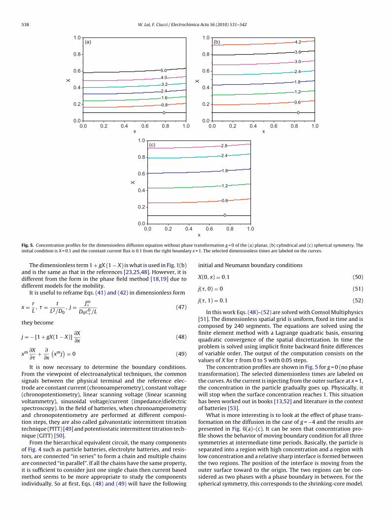
ig. 5. Concentration profiles for the dimensionless diffusion equation without phnitial condition is X = 0.1 and the constant current flux is 0.1 from the right bounda

The dimensionless term 1 + gX (1 − X) is what is used in Fig. 1(b)nd is the same as that in the references [23,25,48]. However, it isifferent from the form in the phase field method [18,19] due toifferent models for the mobility.

It is useful to reframe Eqs. (41) and (42) in dimensionless form

= r

L, � = t

L2/D0, j = Jm+

D0c0+/L(47)

hey become

= − [1 + gX(1 − X)]∂X

∂x(48)

m ∂X

∂�+ ∂

∂x

(xmj

)= 0 (49)

It is now necessary to determine the boundary conditions.rom the viewpoint of electroanalytical techniques, the commonignals between the physical terminal and the reference elec-rode are constant current (chronoamperometry), constant voltagechronopotentiometry), linear scanning voltage (linear scanningoltammetry), sinusoidal voltage/current (impedance/dielectricpectroscopy). In the field of batteries, when chronoamperometrynd chronopotentiometry are performed at different composi-ion steps, they are also called galvanostatic intermittent titrationechnique (PITT) [49] and potentiostatic intermittent titration tech-ique (GITT) [50].

From the hierarchical equivalent circuit, the many componentsf Fig. 4 such as particle batteries, electrolyte batteries, and resis-

ors, are connected “in series” to form a chain and multiple chainsre connected “in parallel”. If all the chains have the same property,t is sufficient to consider just one single chain then current based

ethod seems to be more appropriate to study the componentsndividually. So at first, Eqs. (48) and (49) will have the following

nsformation g = 0 of the (a) planar, (b) cylindrical and (c) spherical symmetry. The1. The selected dimensionless times are labeled on the curves.

initial and Neumann boundary conditions

X(0, x) = 0.1 (50)

j(�, 0) = 0 (51)

j(�, 1) = 0.1 (52)

In this work Eqs. (48)–(52) are solved with Comsol Multiphysics[51]. The dimensionless spatial grid is uniform, fixed in time and iscomposed by 240 segments. The equations are solved using thefinite element method with a Lagrange quadratic basis, ensuringquadratic convergence of the spatial discretization. In time theproblem is solved using implicit finite backward finite differencesof variable order. The output of the computation consists on thevalues of X for � from 0 to 5 with 0.05 steps.

The concentration profiles are shown in Fig. 5 for g = 0 (no phasetransformation). The selected dimensionless times are labeled onthe curves. As the current is injecting from the outer surface at x = 1,the concentration in the particle gradually goes up. Physically, itwill stop when the surface concentration reaches 1. This situationhas been worked out in books [13,52] and literature in the contextof batteries [53].

What is more interesting is to look at the effect of phase trans-formation on the diffusion in the case of g = −4 and the results arepresented in Fig. 6(a)–(c). It can be seen that concentration pro-file shows the behavior of moving boundary condition for all threesymmetries at intermediate time periods. Basically, the particle isseparated into a region with high concentration and a region with

low concentration and a relative sharp interface is formed betweenthe two regions. The position of the interface is moving from theouter surface toward to the origin. The two regions can be con-sidered as two phases with a phase boundary in between. For thespherical symmetry, this corresponds to the shrinking-core model.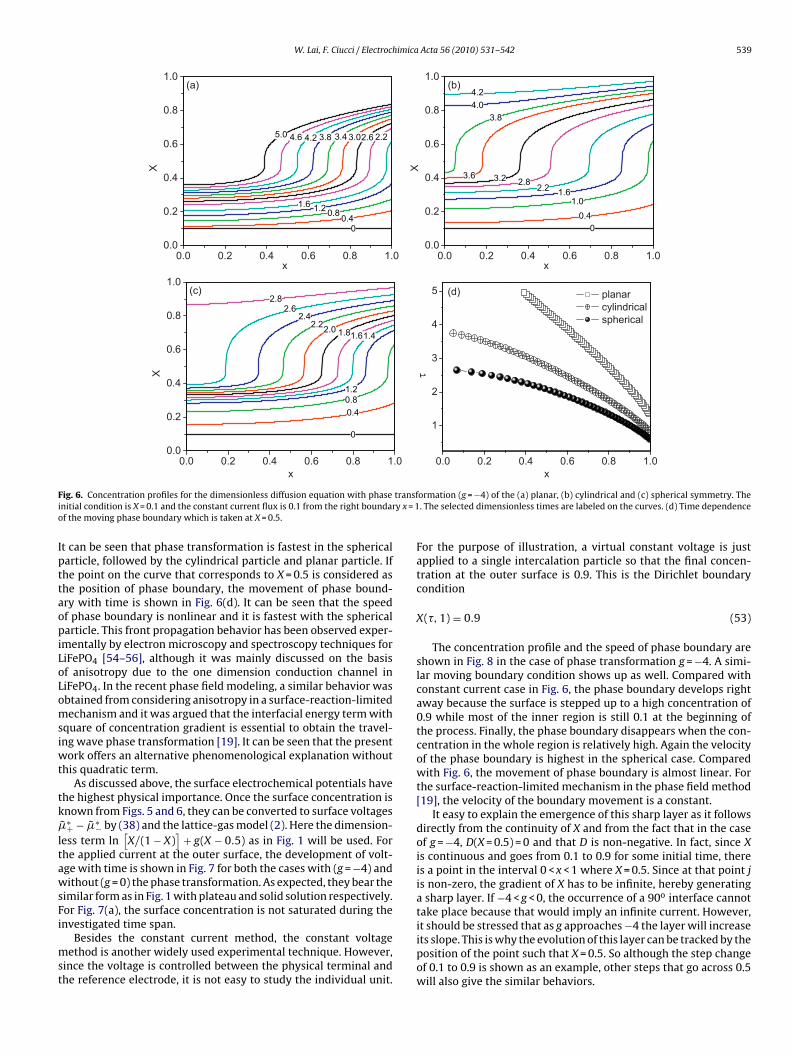

W. Lai, F. Ciucci / Electrochimica Acta 56 (2010) 531–542 539

F transfi y x = 1o

IpttaopiLoLomsiwt

tk�

ltawsFi

mst

ig. 6. Concentration profiles for the dimensionless diffusion equation with phasenitial condition is X = 0.1 and the constant current flux is 0.1 from the right boundarf the moving phase boundary which is taken at X = 0.5.

t can be seen that phase transformation is fastest in the sphericalarticle, followed by the cylindrical particle and planar particle. Ifhe point on the curve that corresponds to X = 0.5 is considered ashe position of phase boundary, the movement of phase bound-ry with time is shown in Fig. 6(d). It can be seen that the speedf phase boundary is nonlinear and it is fastest with the sphericalarticle. This front propagation behavior has been observed exper-

mentally by electron microscopy and spectroscopy techniques foriFePO4 [54–56], although it was mainly discussed on the basisf anisotropy due to the one dimension conduction channel iniFePO4. In the recent phase field modeling, a similar behavior wasbtained from considering anisotropy in a surface-reaction-limitedechanism and it was argued that the interfacial energy term with

quare of concentration gradient is essential to obtain the travel-ng wave phase transformation [19]. It can be seen that the present

ork offers an alternative phenomenological explanation withouthis quadratic term.

As discussed above, the surface electrochemical potentials havehe highest physical importance. Once the surface concentration isnown from Figs. 5 and 6, they can be converted to surface voltages

˜ ∗+ − �̃∗− by (38) and the lattice-gas model (2). Here the dimension-ess term ln

[X/(1 − X)

]+ g(X − 0.5) as in Fig. 1 will be used. For

he applied current at the outer surface, the development of volt-ge with time is shown in Fig. 7 for both the cases with (g = −4) andithout (g = 0) the phase transformation. As expected, they bear the

imilar form as in Fig. 1 with plateau and solid solution respectively.or Fig. 7(a), the surface concentration is not saturated during the

nvestigated time span.

Besides the constant current method, the constant voltageethod is another widely used experimental technique. However,

ince the voltage is controlled between the physical terminal andhe reference electrode, it is not easy to study the individual unit.

ormation (g = −4) of the (a) planar, (b) cylindrical and (c) spherical symmetry. The. The selected dimensionless times are labeled on the curves. (d) Time dependence

For the purpose of illustration, a virtual constant voltage is justapplied to a single intercalation particle so that the final concen-tration at the outer surface is 0.9. This is the Dirichlet boundarycondition

X(�, 1) = 0.9 (53)

The concentration profile and the speed of phase boundary areshown in Fig. 8 in the case of phase transformation g = −4. A simi-lar moving boundary condition shows up as well. Compared withconstant current case in Fig. 6, the phase boundary develops rightaway because the surface is stepped up to a high concentration of0.9 while most of the inner region is still 0.1 at the beginning ofthe process. Finally, the phase boundary disappears when the con-centration in the whole region is relatively high. Again the velocityof the phase boundary is highest in the spherical case. Comparedwith Fig. 6, the movement of phase boundary is almost linear. Forthe surface-reaction-limited mechanism in the phase field method[19], the velocity of the boundary movement is a constant.

It easy to explain the emergence of this sharp layer as it followsdirectly from the continuity of X and from the fact that in the caseof g = −4, D(X = 0.5) = 0 and that D is non-negative. In fact, since Xis continuous and goes from 0.1 to 0.9 for some initial time, thereis a point in the interval 0 < x < 1 where X = 0.5. Since at that point jis non-zero, the gradient of X has to be infinite, hereby generatinga sharp layer. If −4 < g < 0, the occurrence of a 90o interface cannottake place because that would imply an infinite current. However,

it should be stressed that as g approaches −4 the layer will increaseits slope. This is why the evolution of this layer can be tracked by theposition of the point such that X = 0.5. So although the step changeof 0.1 to 0.9 is shown as an example, other steps that go across 0.5will also give the similar behaviors.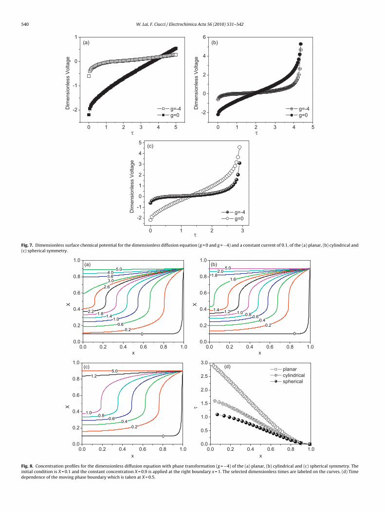

540 W. Lai, F. Ciucci / Electrochimica Acta 56 (2010) 531–542

Fig. 7. Dimensionless surface chemical potential for the dimensionless diffusion equation (g = 0 and g = −4) and a constant current of 0.1, of the (a) planar, (b) cylindrical and(c) spherical symmetry.

Fig. 8. Concentration profiles for the dimensionless diffusion equation with phase transformation (g = −4) of the (a) planar, (b) cylindrical and (c) spherical symmetry. Theinitial condition is X = 0.1 and the constant concentration X = 0.9 is applied at the right boundary x = 1. The selected dimensionless times are labeled on the curves. (d) Timedependence of the moving phase boundary which is taken at X = 0.5.

W. Lai, F. Ciucci / Electrochimica Acta 56 (2010) 531–542 541

F −4) uc a), (b)

itlawbiF

raicfd(cratAsspt

tebctf

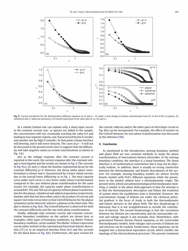
ig. 9. Current waveforms for the dimensionless diffusion equation (g = 0 and g =ylindrical and (c) spherical symmetry. (d) Cottrell expression of the same data in (

In a similar fashion one can explain why a sharp layer occursn the constant current case: as species are added to the sample,he concentration will rise, eventually reaching the value 0.5 andeading to two separate regions, one characterized by low X (inside)nd another one by high X (outside). At that point a sharp interfaceill develop, and it will move inwards. The cases of g < −4 will not

e discussed in the present work since it suggests that the diffusiv-ty will take negative values at certain concentrations as shown inig. 1(b).

Just as the voltage response after the constant current iseported in this work, the current response after the constant volt-ge is investigated and the results are shown in Fig. 9. The currentsn Fig. 9(a), (b) and (c) show the familiar exponential decay for theonstant diffusivity g = 0. However, the decay under phase trans-ormation is slower and is characterized by a lower initial current,ue to the overall lower diffusivity as in Fig. 1. The total capacityarea under each curve) is also lower under phase transformationompared to the case without phase transformation for the sameeason. For example, the capacity under phase transformation isround 84%, 76% and 70% out of capacity without phase transforma-ion for the planar, cylindrical and spherical geometry respectively.nother plot that has been often used is the product of current andquare root time versus time so that Cottrell behavior for the planarymmetry can be observed, which is a plateau at the short time. Thislot is shown in Fig. 9(d). The Cottrell behavior is observed for bothhe constant diffusivity and the one with phase transformation.

Finally, although only constant current and constant concen-ration boundary conditions on the surface are shown here as

xamples, other types of boundary conditions, e.g. Butler–Volmeroundary condition, can be studied. This Butler–Volmer expressionan be either written in the conventional form from kinetic deriva-ion [57] or in an empirical function form [41] and this accountor the black boxes in Fig. 4(b). Furthermore, the pure resistor for

nder a step change of surface concentration from 0.1 to 0.9 of the (a) planar, (b)and (c).

the current collector and/or the other parts of electrolyte circuit inFig. 4(b) can be incorporated. For example, the effect of resistor onthe Cottrell behavior for non-phase-transformation was discussedin the reference [58].

5. Conclusion

As mentioned in the introduction, moving boundary methodand phase field are two common methods to study the phasetransformation of intercalation battery electrodes. In the movingboundary condition, the interface is a sharp boundary. The sharpinterface is of mathematical convenience but it may not be phys-ically realistic. In addition, there is usually no strong connectionbetween the thermodynamic and kinetic descriptions of the sys-tem. For example, moving boundary models are almost strictlykinetic models with Fick’s diffusion equations while the param-eters in the models seldom have a thermodynamic origin. Thepresent work, which uses phenomenological thermodynamic mod-eling, is similar to the phase field approach in that the attempt isto find the thermodynamic description and follow the evolutionof system when the equilibrium state is disturbed. However, theconcentration change of lithium ion under the chemical poten-tial gradient is the focus of study in both the thermodynamicand kinetic pictures in the phase field. The first disadvantage isobviously that it is not straightforward to include the contribu-tion of electron. The second disadvantage is that the correlationbetween the lithium ion concentration and the measureable cur-rent and voltage signals is not normally clear. Nonetheless, with

generalized Poisson–Nernst–Planck equations as the irreversiblethermodynamic models, both voltages and currents of lithium ionand electron can be tracked. Furthermore, these equations can bemapped into a hierarchical equivalent circuit, which clarifies thetopology of the electrochemical processes. The present treatment

5 himica

atlHgcdlshddo

A

p

R

[[

[[

[

[[[

[

[

[

[[

[

[[[[[[[[[[[[[

[[[[

[[

[

[[[[[[

[[[

[[

[Tarascon, Chem. Mater. 18 (2006) 5520–5529.

42 W. Lai, F. Ciucci / Electroc

lso differs from the phase field method in the detailed implemen-ation of thermodynamic and kinetic equations. First, the presentattice-gas model does not have the interfacial energy term in Cahn-illiard equation. Second, the mobility term also follows the lattice-as model while the mobility in the phase field is assumed to be aonstant. While it can be argued that the present thermodynamicescription is not as complete as the phase field model, the present

attice-gas model has the technical advantage of mathematicalimplicity because no fourth-order partial differential equationsave to be solved. Furthermore, this approach leads to a simpleimensionless diffusion equation with concentration dependentiffusivity. This equation serves as a model to understand the effectf phase transformation on different electrochemical processes.

cknowledgement

W.L. would like to acknowledge Michigan State University forroviding the start-up package.

eferences

[1] T. Ohzuku, M. Kitagawa, T. Hirai, J. Electrochem. Soc. 137 (1990) 769–775.[2] M.M. Thackeray, Prog. Solid State Chem. 25 (1997) 1–71.[3] T. Ohzuku, A. Ueda, N. Yamamoto, J. Electrochem. Soc. 142 (1995) 1431–1435.[4] T. Ohzuku, A. Ueda, J. Electrochem. Soc. 144 (1997) 2780–2785.[5] J.R. Dahn, Phys. Rev. B 44 (1991) 9170–9177.[6] T. Ohzuku, Y. Iwakoshi, K. Sawai, J. Electrochem. Soc. 140 (1993) 2490–2498.[7] A.K. Padhi, K.S. Nanjundaswamy, J.B. Goodenough, J. Electrochem. Soc. 144

(1997) 1188–1194.[8] N. Meethong, H.Y.S. Huang, W.C. Carter, Y.M. Chiang, Electrochem. Solid State

Lett. 10 (2007) A134–A138.[9] V. Srinivasan, J. Newman, J. Electrochem. Soc. 151 (2004) A1517–A1529.10] Q. Zhang, R.E. White, J. Electrochem. Soc. 154 (2007) A587–A596.11] U.S. Kasavajjula, C.S. Wang, P.E. Arce, J. Electrochem. Soc. 155 (2008)

A866–A874.12] T.C. Illingworth, I.O. Golosnoy, J. Comput. Phys. 209 (2005) 207–225.13] J. Crank, The Mathematics of Diffusion, 2nd ed., Oxford University Press, New

York, NY, 1980.14] M.J. Baines, M.E. Hubbard, P.K. Jimack, R. Mahmood, Commun. Comput. Phys.

6 (2009) 595–624.15] K. Jagannathan, J. Electrochem. Soc. 156 (2009) A1028–A1033.

16] K. Thornton, J. Agren, P.W. Voorhees, Acta Mater. 51 (2003) 5675–5710.17] W.J. Boettinger, J.A. Warren, C. Beckermann, A. Karma, Annu. Rev. Mater. Res.

32 (2002) 163–194.18] B.C. Han, A. Van der Ven, D. Morgan, G. Ceder, Electrochim. Acta 49 (2004)

4691–4699.19] G.K. Singh, G. Ceder, M.Z. Bazant, Electrochim. Acta 53 (2008) 7599–7613.

[

[

[

Acta 56 (2010) 531–542

20] M. Tang, H.Y. Huang, N. Meethong, Y.H. Kao, W.C. Carter, Y.M. Chiang, Chem.Mater. 21 (2009) 1557–1571.

21] J.W. Cahn, J.E. Hilliard, J. Chem. Phys. 28 (1958) 258–267.22] T.L. Hill, An Introduction to Statistical Thermodynamics, Dover Publications,

New York, NY, 1987.23] W.R. McKinnon, R.R. Haering, Modern Aspects of Electrochemistry, vol. 15,

Plenum Press, New York, NY, 1983.24] S.T. Coleman, W.R. McKinnon, J.R. Dahn, Phys. Rev. B 29 (1984) 4147–4149.25] M.D. Levi, D. Aurbach, Electrochim. Acta 45 (1999) 167–185.26] J. Jamnik, J. Maier, Phys. Chem. Chem. Phys. 3 (2001) 1668–1678.27] W. Lai, S.M. Haile, J. Am. Ceram. Soc. 88 (2005) 2979–2997.28] J. Bisquert, Phys. Chem. Chem. Phys. 10 (2008) 49–72.29] Y. Gao, J.N. Reimers, J.R. Dahn, Phys. Rev. B 54 (1996) 3878–3883.30] P.A. Derosa, P.B. Balbuena, J. Electrochem. Soc. 146 (1999) 3630–3638.31] S.W. Kim, S.I. Pyun, Electrochim. Acta 46 (2001) 987–997.32] K.N. Jung, S. Pyun, S.W. Kim, J. Power Sources 119 (2003) 637–643.33] J. Bisquert, V.S. Vikhrenko, Electrochim. Acta 47 (2002) 3977–3988.34] M.W. Verbrugge, B.J. Koch, J. Electrochem. Soc. 150 (2003) A374–A384.35] D.K. Karthikeyan, G. Sikha, R.E. White, J. Power Sources 185 (2008) 1398–1407.36] S. Selberherr, Analysis and Simulation of Semiconductor Devices, Springer, New

York, 1984.37] R.S. Eisenberg, J. Membr. Biol. 150 (1996) 1–25.38] M.Z. Bazant, K. Thornton, A. Ajdari, Phys. Rev. E 70 (2004).39] R.P. Buck, J. Membr. Sci. 17 (1984) 1–62.40] J. Horno, A.A. Moya, C.F. GonzalezFernandez, J. Electroanal. Chem. 402 (1996)

73–80.41] W. Lai, S.M. Haile, Phys. Chem. Chem. Phys. 10 (2008) 865–883.42] F. Ciucci, Y. Hao, D.G. Goodwin, Phys. Chem. Chem. Phys. 11 (2009)

11243–11257.43] S.R. De Groot, P. Mazur, Non-Equilibrium Thermodynamics, Dover Publications,

Mineola, NY, 1984.44] R.P. Buck, C. Mundt, Electrochim. Acta 44 (1999) 1999–2018.45] A.A. Moya, J. Castilla, J. Horno, J. Phys. Chem. 99 (1995) 1292–1298.46] G. Oster, A. Perelson, A. Katchals, Nature 234 (1971) 393–399.47] W. Lai, F. Ciucci, submitted.48] M.W. Verbrugge, B.J. Koch, J. Electrochem. Soc. 146 (1999) 833–839.49] C.J. Wen, B.A. Boukamp, R.A. Huggins, W. Weppner, J. Electrochem. Soc. 126

(1979) 2258–2266.50] W. Weppner, R.A. Huggins, J. Electrochem. Soc. 124 (1977) 1569–1578.51] COMSOL Multiphysics, 1997–2010 COMSOL AB.52] H.S. Carslaw, J.C. Jaeger, Conduction of Heat in Solids, second ed., Oxford Uni-

versity Press, New York, NY, 1986.53] S. Atlung, K. West, T. Jacobsen, J. Electrochem. Soc. 126 (1979) 1311–1321.54] G.Y. Chen, X.Y. Song, T.J. Richardson, Electrochem. Solid State Lett. 9 (2006)

A295–A298.55] L. Laffont, C. Delacourt, P. Gibot, M.Y. Wu, P. Kooyman, C. Masquelier, J.M.

56] C. Delmas, M. Maccario, L. Croguennec, F. Le Cras, F. Weill, Nat. Mater. 7 (2008)665–671.

57] A.J. Bard, L.R. Faulkner, Electrochemical methods: Fundamentals and Applica-tions, second ed., John Wiley & Sons, Inc., New York, NY, 2000.

58] C. Montella, J. Electroanal. Chem. 518 (2002) 61–83.