THERMO ECONOMIC ANALYSIS OF A FRENCH FRIES PROCESSING

THERMO-ECONOMIC ANALYSIS OF A FRENCH FRIES PROCESSING

PLANT AT LAMBERT’S BAY

JOHAN POTGIETER

THESIS PRESENTED FOR THE DEGREE OF

MSCENG IN MECHANICAL ENGINEERING AT THE UNIVERSITY OF

STELLENBOSCH

THESIS SUPERVISOR: DR T.M. HARMS

DECEMBER 2004

ii

DECLARATION

I, Johan Potgieter, submit this thesis in fulfilment of the requirements of the degree of Master

of Science in Engineering. I claim that this is my original work and that it has not been

submitted in this or in a similar form for a degree at any other university.

___________________

J. Potgieter BEng (Mechanical)

____ day of ________ 2004

iii

ABSTRACT

In the literature study energy efficiency is discussed in general, as well as certain critical areas

of importance to this study. In addition, measuring and monitoring equipment, and energy

inefficiencies in steam and refrigeration systems are reviewed briefly.

In the energy analysis, an energy audit strategy is discussed in general. A walkthrough audit

of the plant was conducted with specific focus on visible losses in the steam, refrigeration and

production line systems. An energy analysis, as discussed in Chapter 3, indicates the main

energy consumers, with steam being the biggest consumer of energy.

The main consumers of refrigeration energy are the cold stores, flow freezer and blast freezer.

Energy consumption in the cold stores can be minimised mechanically, while refrigeration

energy of the flow freezer and blast freezer can be minimised through the modification of

production activity.

The main consumers of steam at the processing plant are the dryers, oil fryer, blanchers and

steam peeler. Improved energy savings at the dryers can be obtained through optimisation of

moisture and heat transfer mechanisms, while the energy of the blanchers and steam peeler

can be combined by means of heat exchangers. The transfer of waste energy by means of a

finned-tube heat exchanger from the steam peeler to the blanchers was investigated.

The newly installed coal boiler shows capacity for improving the quality of steam, as well as

efficiency, by incorporating an economiser and separator for improving steam quality,

automatic TDS control and blow-down heat recovery.

The product life cycle is discussed considering future automation that could lead to energy

and labour savings.

Lastly the utilisation of product waste as a future research subject is discussed.

A confidentiality agreement was entered into with Oceana.

iv

OPSOMMING

In die literatuurstudie word energie-effektiwiteit oor die algemeen bespreek, asook sekere

kritieke areas wat vir die ondersoek van belang is. Hierbenewens word meettoerusting

vlugtig bespreek, asook energie-oneffektiwiteite in die verkoeling- en stoomstelsels.

In die energie-ontleding word ’n energie-ouditstrategie in die breë bespreek. ’n Deurstap-

oudit van die aanleg is uitgevoer met spesifieke fokus op sigbare verliese in die

verkoelingstelsel, stoomstelsel en produksielyn. Die samestelling van energieverbruik in die

aanleg word uiteengesit in Hoofstuk 3, waar dan ook aangedui word dat stoom die grootste

energieverbruiker is.

Die hoofverbruikers van verkoelingsenergie is die koelkamers, die deurvloei-vrieskamer en

die blitsvrieskamer. By die koelkamers kan verliese meganies geminimeer word, terwyl

veranderinge aan produksie-aktiwiteite energieverbruik by die deurvloei-vrieskamer en die

blitsvrieskamer kan verlaag.

Die hoofverbruikers van stoom by die verwerkingsaanleg is die droërs, oliebraaier,

blansjeerders en stoomskiller. Energie-effektiwiteit by die droërs kan verhoog word deur

vog- en warmte-oordrag optimaal te laat plaasvind deur korrekte instandhoudingsprosedures.

Energieverbruik by die stoomskiller en blansjeerders kan deur middel van warmteruilers

gekombineer word. ’n Ondersoek na die energie-integrasie van die stoomskiller en die

blansjeerders is dan ook uitgevoer. Die pas geïnstalleerde steenkoolketel toon ruimte vir die

verhoging van energie-effektiwiteit deur die daarstel van ’n ekonomiseerder – ’n skeier wat

die gehalte van die stoom verbeter, outomatiese TDS-beheer en afblaasherwinning.

Die produk se lewensiklus word bespreek ten einde toekomstige outomatisering te motiveer in

terme van energie- en arbeideffektiwiteit, asook die uitskakeling van onnodige blootstelling

van die produk aan omgewingstemperature.

Laastens word die herwinning van afvalstowwe as ’n toekomstige navorsingsprojek bespreek.

’n Vertroulikheidsooreenkoms is met Oceana gesluit en word eerbiedig.

v

ACKNOWLEDGEMENT

I would like to thank Dr Thomas Harms, my promotor, for his mentorship and availability.

His guidance was of enormous value.

I would also like to thank Koos van Wyk, Plant Engineer at Lambert’s Bay, for his assistance

and willingness to help. Without this, data collection and access to certain information would

have been much more difficult. His willingness to make the plant available for an energy

analysis illustrates his valuable contribution.

vi

CONTENTS

DECLARATION ................................................................................................... II

ABSTRACT .........................................................................................................III

OPSOMMING ......................................................................................................IV

ACKNOWLEDGEMENT ....................................................................................V

LIST OF FIGURES ..............................................................................................IX

LIST OF TABLES ................................................................................................XI

LIST OF SYMBOLS ........................................................................................XIII

1 INTRODUCTION............................................................................................1

1.1 Energy Efficiency as National Interest......................................................................... 1

1.2 Energy Efficiency in the French Fries Processing Industry ........................................ 1

2 LITERATURE STUDY ...................................................................................2

2.1 Energy Efficiency......................................................................................................... 2

2.1.1 The Energy Efficiency Earnings Strategy................................................................ 2

2.2 Energy Efficiency Analysis of Food Processing Facility............................................. 5

2.2.1 Walkthrough Audit................................................................................................... 5

2.2.2 Diagnostic Audit ...................................................................................................... 6

2.2.3 General Energy Audit............................................................................................... 6

2.2.4 Energy Audit of Steam............................................................................................. 8

2.2.5 Energy Audit of Refrigeration................................................................................ 16

2.2.6 Measuring Instrumentation .................................................................................... 34

3 LAMBERT’S BAY ENERGY ANALYSIS .................................................38

3.1 Energy Analysis Strategy ........................................................................................... 38

3.2 Plant Layout ............................................................................................................... 38

3.3 Walkthrough Audit..................................................................................................... 39

3.4 Energy Consumption.................................................................................................. 40

3.5 Economic Decision Analysis Approach..................................................................... 42

3.6 Steam ......................................................................................................................... 44

3.6.1 Dryers .................................................................................................................... 44

3.6.2 Boiler ..................................................................................................................... 51

3.6.3 Utilisation of Reject Steam at Steam Peeler........................................................... 55

3.6.4 Steam Pipes ............................................................................................................ 70

vii

3.7 Refrigeration............................................................................................................... 74

3.7.1 Weather Correlations.............................................................................................. 74

3.7.2 Cold Stores ............................................................................................................ 78

3.7.3 Flow Freezer........................................................................................................... 86

3.7.4 Blast Freezer........................................................................................................... 87

3.7.5 Refrigeration Pipes ................................................................................................ 87

3.8 Product Lifecycle Analysis ........................................................................................ 89

3.9 Waste Utilisation ....................................................................................................... 92

4 CONCLUSION ..............................................................................................94

REFERENCES......................................................................................................95

BIBLIOGRAPHY .................................................................................................98

A APPENDIX: ELECTRICITY, COAL AND PRODUCTION RECORDS ...100

A.1 Electricity Readings ................................................................................................ 101

A.2 Electricity and Coal Consumption .......................................................................... 102

A.3 Electricity, Coal and Production Comparison.......................................................... 103

A.4 Walkthrough Audit Checklist .................................................................................. 104

B APPENDIX: NORTIER TEMPERATURE AND HUMIDITY DATA ......105

B.1 Nortier Temperature Data............................................................................................. 106

B.2 Nortier Humidity Data.................................................................................................. 111

C APPENDIX: AMMONIA REFRIGERATION ............................................116

C.1 Ammonia Refrigeration Pipes ................................................................................. 117

D APPENDIX: CALCULATIONS FOR UNLAGGED STEAM PIPING ......125

D.1 Calculations for Unlagged Steam Piping .................................................................... 126

D.1.1 Natural Convection over Horizontal Cylinder ..................................................... 126

D.1.2 Natural Convection over Vertical Wall ................................................................ 128

E APPENDIX: HEAT LOAD CALCULATIONS FOR INSULATION

PANELS..............................................................................................................134

E.1 Calculation of Heating Load on Outside Panels of Cooling Room ............................. 135

F APPENDIX: COLD STORE CALCULATIONS .........................................143

F.1 Cold Store Calculations ................................................................................................ 144

F.1.1 Infiltration Effect ................................................................................................... 144

F.1.2 Mass Transfer......................................................................................................... 151

viii

G APPENDIX: PAYBACK CALCULATIONS FOR AIR CURTAINS FOR

COLD STORES .................................................................................................162

G.1 Payback Calculations of Air Curtains for Cold Stores ................................................ 163

H APPENDIX: INVESTIGATION OF IMPROVEMENT OF STEAM

UTILISATION....................................................................................................166

H.1 Investigation of Steam Utilisation Improvement ........................................................ 167

H.1.1 Steam Peeler ......................................................................................................... 167

I APPENDIX: CALCULATIONS FOR INSTALLATION OF OPTICAL

SORTER IN PRODUCTION LINE ..................................................................171

I.1 Calculations for Installation of Optical Sorter in Production Line ............................... 172

I.1.1 Conclusion .............................................................................................................. 176

J APPENDIX: DRYER TEST MEASUREMENTS AND CALCULATIONS 179

J.1 Dryer Test Measurements ............................................................................................. 180

J.2 Dryer Test Calculations ................................................................................................ 181

K APPENDIX: VISUAL BASIC PROGRAM FOR HEAT EXCHANGER

ANALYSIS ........................................................................................................183

K.1 Heat Exchanger Code .................................................................................................. 184

K.2 Heat Exchanger Program Form ................................................................................... 198

K.3 Correlations for Steam and Water Properties............................................................... 199

ix

LIST OF FIGURES

Figure 1: Sankey diagram for a small factory, indicating the energy flow................................... 4

Figure 2: Boiler inputs and losses ................................................................................................. 9

Figure 3: Typical vapour compression cycle .............................................................................. 17

Figure 4: Simple vapour-compression cycle............................................................................... 19

Figure 5: Schematic representation of ammonia refrigeration plant........................................... 20

Figure 6: T-s diagram for vapour-compression cycle with flash chamber ................................. 21

Figure 7: h-s diagram of an adiabatic compressor ...................................................................... 23

Figure 8: Evaporative condenser................................................................................................. 27

Figure 9: Principle of operation of the absorption dehumidifier................................................. 31

Figure 10: Dessicant dehumidifier operation .............................................................................. 32

Figure 11: Infiltration .................................................................................................................. 34

Figure 12: Schematic representation of plant layout................................................................... 38

Figure 13: Pie chart indicating the main steam users.................................................................. 40

Figure 14: Electricity consumption of various users................................................................... 41

Figure 15: Sankey diagram of total energy flow in plant............................................................ 42

Figure 16: Schematic drawing of dryer illustrating airflow........................................................ 44

Figure 17: Dry and wet-bulb temperatures of each section ........................................................ 45

Figure 18: Specific humidity of air through each section ........................................................... 45

Figure 19: Relative humidity of air through each section........................................................... 46

Figure 20: Mass transfer of water from fries to air ..................................................................... 46

Figure 21: Adiabatic saturation of air ......................................................................................... 47

Figure 22: Flash-steam heat recovery system with plate heat exchanger ................................... 53

Figure 23: Rejected steam of steam peeler into atmosphere ....................................................... 56

Figure 24: Steam peeler energy flow .......................................................................................... 57

Figure 25: Schematic representation of steam peeler current operation ..................................... 59

Figure 26: Steam peeler with shell-tube heat exchanger............................................................. 59

Figure 27: Control volume for finned tube ................................................................................. 60

Figure 28: Tube bank configuration of heat exchanger .............................................................. 67

Figure 29: Heat transfer for rectangular heat exchanger concept ............................................... 67

Figure 30: Heat transfer for rectangular heat exchanger with 35 layers ..................................... 68

x

Figure 31: Dry-bulb temperature comparison............................................................................. 75

Figure 32: Humidity comparison ................................................................................................ 75

Figure 33: Temperature difference correlation ........................................................................... 76

Figure 34: Average correlated temperature for plant .................................................................. 77

Figure 35: Humidity difference correlation ................................................................................ 77

Figure 36: Average correlated humidity ratio for plant .............................................................. 78

Figure 37: Cold stores and airlock .............................................................................................. 79

Figure 38: Insulating panel with indication of temperature gradient .......................................... 80

Figure 39: Infiltration effect ........................................................................................................ 84

Figure 40: Schematic representation of flow freezer .................................................................. 86

Figure 41: Production process line.............................................................................................. 90

Figure 42: Production line with optical sorter modification ....................................................... 91

Figure 43: Potato waste from steam peeler at plant .................................................................... 92

Figure D. 1: Convection heat loss: variable pipe diameter .....................................................129

Figure D. 2: Radiation heat loss: variable temperature ...........................................................131

Figure F. 1: Schematic representation of heat transfer of cold store........................................144

Figure F. 2: Schematic drawing of vapour transfer phenomena .............................................152

Figure I. 1: Production line with optical sorter inserted ..........................................................172

Figure K. 1: Heat exchanger program form ............................................................................198

xi

LIST OF TABLES

Table 3. 1: Percentage loss of product mass .............................................................................57

Table 3. 2: Heat exchanger simulation results for 50 layers .....................................................68

Table 3. 3: Heat exchanger simulation results for 35 layers .....................................................69

Table 3. 4: Payback periods for heat exchanger configuration .................................................70

Table A. 1: Electricity readings and coal usage ...................................................................... 101

Table A. 2: Electricity and coal consumption data for January 2002 till May 2002 ............... 102

Table A. 3: Electricity, coal and production for January 2002 till May 2002 ........................ 103

Table B. 1: Nortier temperature data .......................................................................................110

Table B. 2: Nortier humidity data ...........................................................................................115

Table C. 1: Dimensional properties of segment 1 ...................................................................117

Table C. 2: Sizes of isothermal areas in segment 1..................................................................117


Table C. 4: Sizes of isothermal areas in segment 2 .................................................................118


Table C. 6: Sizes of isothermal areas in segment 3..................................................................118

Table C. 7: Area summation for isothermal areas....................................................................118

Table C. 8: Thermal properties of air ......................................................................................119

Table C. 9: Temperature differences for isothermal areas ......................................................119

Table C. 10: Convection heat transfer for segment 1 areas at 0 oC..........................................119





Table C. 15: Convection heat transfer for segment 3 areas at 11 oC........................................122

Table C. 16: Average unit price for plant electricity use ........................................................123

Table C. 17: Payback period calculation .................................................................................124

Table C. 18: MathCAD calculations to calculate capital ........................................................124

Table D. 1: Dimensional and thermal properties of pipe and plant atmosphere .....................126

xii

Table D. 2: Radiation properties of stainless steel ..................................................................130

Table E. 1: Dimensional properties of insulation panel ..........................................................135

Table E. 2: Temperature measurements and atmospheric conditions .....................................135

Table E. 3: Radiation properties of insulation panel ...............................................................135

Table E. 4: Coefficients for calculation of saturated vapour pressure ....................................136

Table E. 5: Properties of insulation panel ...............................................................................141

Table F. 1: Plant and cold store conditions .............................................................................145

Table F. 2: Constants for saturated vapour pressure ...............................................................145

Table F. 3: Constants to determine dewpoint temperature ......................................................147

Table F. 4: Specific enthalpy values for dry air and water vapour .........................................149

Table F. 5: Equations to determine wet-bulb temperature ......................................................149

Table F. 6: Calculation of specific and relative humidity of passage air ................................150

Table F. 7: Dimensional properties of door ............................................................................155

Table F. 8: Average temperatures for a year ...........................................................................155

Table F. 9: Calculation of specific and relative humidity of passage air ................................157

Table H. 1: Steam cost savings calculations ...........................................................................169

Table I. 1: Product temperatures on production line ...............................................................173

Table I. 2: Energy savings calculations for dryer ....................................................................175

Table I. 3: Energy savings calculations for fryer ....................................................................175

Table I. 4: Energy savings calculations for flow freezer .........................................................175

Table I. 5: Energy savings calculation table ...........................................................................177

Table I. 6: Sorting line savings ................................................................................................178

Table J. 1: Dryer test measurements .......................................................................................180

Table J. 2: Dryer spreadsheet test calculations .......................................................................182

xiii

LIST OF SYMBOLS

A Single payment in a series of n equal payments [R]

Ao Outside area [m2]

Ai Inside area [m2]

Afr Frontal area [m2]

COP Coefficient of Performance

COPR Coefficient of Performance for Refrigerator

COPRNH3 Coefficient of Performance for Ammonia Refrigerator

cplugin Specific heat of dry air in [J/kgK]

cpluguit Specific heat of dry air out [J/kgK]

cpvlugin Specific heat of saturated water in [J/kgK]

cpvluguit Specific heat of saturated water out [J/kgK]

D Diffusion coefficient [kg/ms]

D Diameter [m]

ef Fin effectiveness

insteamE ,& Energy flowrate of steam in [kW]

outsteamE ,& Energy flowrate of steam out [kW]

inproductE ,& Energy flowrate of product in [kW]

outproductE ,& Energy flowrate of product out [kW]

F Future value [R]

F Friction factor for smooth walls

G Mass flux [kg/m2s]

H Specific enthalpy [kJ/kg]

ha Specific enthalpy of dry air [kJ/kg]

hd Mass transfer coefficient [kg/m2s]

hevapin Specific enthalpy of evaporator working fluid in [kJ/kg]

hevapout Specific enthalpy of evaporator working fluid out [kJ/kg]

hfby70 Saturation enthalpy of liquid water at 70 oC [kJ/kg]

hg,16bar Saturated specific enthalpy of steam at 16 bar [kJ/kg]

hs Specific enthalpy of steam [kJ/kg]

hw Specific enthalpy of water [kJ/kg]

H Enthalpy flow [W]

xiv

HHV Higher heating value [MJ/kg]

HSUIT Enthalpy of steam out [W]

HWIN Enthalpy of water in [W]

i Interest rate per period

igwo Latent heat of water vapour at a saturation temperature of 0 oC

[J/kg]

K Thermal conductivity coefficient [W/mK]

Kalwaarde Calorific value of heavy fuel oil [J/L]

L Length [m]

fm& Mass flowrate of saturated liquid [kg/s]

gm& Mass flowrate of saturated gas [kg/s]

mHFO Mass flow of heavy fuel oil [kg/hr]

mlugin Mass flow of air in [kg/s]

potatom& Mass flowrate of potatoes [kg/s]

inproductm ,& Mass flowrate of potatoes in [kg/s]

outproductm ,& Mass flowrate of potatoes out [kg/s]

insteamm ,& Mass flowrate of steam in [kg/s]

steamlossm ,& Mass flowrate of steam lost for further heat recovery [kg/s]

muitlaat Mass flow of combustion products [kg/s]

mw Mass flow of water in/steam out [kg/s]

wastem& Mass flowrate of potato waste [kg/s]

Ma Molar mass of air [kg/kmol]

Mv Molar mass of vapour [kg/kmol]

n Number of interest period

NCV Nett calorific value [MJ/kg]

P Present value [R]

P Pressure [Pa]

Patm Atmospheric pressure (101 300 Pa)

Powerideal Ideal power [kW]

Powerreal Real power [kW]

Psat70 Saturation pressure at 70 oC [Pa]

Pr Prandtl number

QE Heat flow of exhaust gases [W]

xv

QH Heat flow from/to warm source/sink [W]

QL Heat flow from/to cold sink/source [W]

QO Heat losses to environment [W]

QV Heat contents of combustion product [W]

QW Heat flow into water [W]

Rlug Specific gas constant of air [J/kgK]

r Radius [m]

ri Inside radius [m]

ro Outside radius [m]

Sh Sherwood number

Sc Schmidt number

T Temperature [K]

TH Temperature at warm source/sink [K]

TL Temperature at cold sink/source [K]

Tlugin Temperature of air in [K]

Tluguit Temperature of air out [K]

U Overall heat transfer coefficient [W/m2K]

Udesign Overall design heat transfer coefficient [W/m2K]

Uactual Overall actual heat transfer coefficient [W/m2K]

VHFO Volume flow of heavy fuel oil [L/hr]

Va Molecular volume of air [m3/kmol]

potatolossV ,& Volume flowrate of lost potatoes [m3/s]

Vv Molecular volume of vapour [m3/kmol]

wa Specific work actual [W/kg]

Wpump Specific work pump [W/kg]

ws Specific work shaft [W/kg]

Wnet,in Specific work net in [W/kg]

W Work [W]

WPUMP Pump work [W]

Yieldalc Alcohol yield [l/ton]

Greek Symbols

Δx Length of segment [m]

xvi

η Efficiency

ηC Carnot efficiency

ηcon Conversion efficiency

ηPlant/System Efficiency factor of plant/system

ηutils Utilisation factor

ρ Density [kg/m3]

ρpotato Density of potatoes [kg/m3]

ρs Density of steam [kg/m3]

ρw Density of water [kg/m3]

μ Dynamic viscosity [Ns/m2]

v Specific volume [kg/m3]

vg,16bar Specific volume of saturated steam at 16 bar [kg/m3]

υ Kinematic viscosity [m2/s]

νfby70 Specific volume of saturated liquid at 70 oC

Φ Relative humidity [kg water vapour/kg water vapour at saturation]

ω Specific humidity [kg vapour/kg dry air]

1

1 INTRODUCTION

1.1 Energy Efficiency as National Interest

A thermo-economic analysis is an efficiency analysis of the application of thermal energy in a

plant. In this document, an approach towards an energy efficiency analysis for a French fries

processing company at Lambert’s Bay, South Africa, is developed.

Energy efficiency is often a neglected income for companies, especially in South Africa,

where energy costs are of the cheapest in the world and the interest rates are high, which

increase payback time. Many people consider the energy efficiency industry to be a billion-

Rand industry, accompanied by many advantages. It was found that safety and production

improve when energy is used more efficiently.

Ghana is already beginning to reap the fruits of its energy efficiency programme, which

started in November 1997. The Executive Director of the independent Ghana Energy

Foundation, Dr Alfred Ofosu-Ahenkorah, states that the primary weapon used to promote the

efficient use of energy is education – making people aware of simple housekeeping measures

– and the second weapon is technology, which, of course, costs money (Zhuwakinyu, 2001).

All of the above strengthens the need for an energy efficiency analysis.

1.2 Energy Efficiency in the French Fries Processing Industry

Most French fries processing plants use the same methods of processing and, thus, more or

less the same energy transport methods. Steam and refrigeration systems are the largest

energy consumers in the French fries industry, therefore the steam and refrigeration system

will be the main focal point in this document.

2

2 LITERATURE STUDY

2.1 Energy Efficiency

Energy is one of the largest controllable costs in most organisations and companies. There is

considerable scope for reducing energy consumption and, therefore, costs. A company should

realise that good housekeeping results in more efficient use of energy, and that company staff

need to be educated before capital is spent on equipment that will improve energy efficiency.

2.1.1 The Energy Efficiency Earnings Strategy

A general energy efficiency earnings strategy was compiled by the Energy Research Institute

(ERI) of the University of Cape Town (The 3E Strategy, How to Save Energy and Money,

2000) to enable companies to determine the energy efficiencies of their energy consumers.

This strategy was modified for the special application required for the French fries processing

industry and, to a certain extent, is employed in this thesis. According to the ERI, the five

fundamental aspects of an energy management strategy are:

i. The need for a company energy efficiency strategy or plan and the basic outline for a

cost reduction program.

ii. Purchase and cost control and a consumption audit of primary energy usage.

iii. Framework and methodology for monitoring and targeting energy savings.

iv. Savings in energy usage through positive practical methods for improving the

efficiency of plant and industrial processes.

v. Financial appraisal of energy efficiency.

The following discussion will explain how this energy efficiency earnings strategy should be

implemented. According to the ERI, energy savings projects may be divided into four

categories:

3

1. Improved housekeeping (maintenance, etc.)

2. Low-cost modifications and improvements

3. Refitting existing systems with new parts and equipment

4. Major capital expenditure

An energy audit of a facility is conducted by means of a walkthrough audit, a diagnostic audit

and the identification of potential energy saving areas.

The walkthrough audit is a tour through the facility or plant, looking for obvious signs of

energy wastage. This audit is more significant when conducted by a person who is familiar

with process insulation and energy management. Typical signs of energy wastage that can be

noticed during a walkthrough audit include missing or damaged insulation, hot or cold

surfaces, wet insulation, deteriorating insulation coverings or protective finishes, missing or

damaged vapour retarders, gaps in insulation at expansion or contracting joints, steam leaks or

visible steam wastages.

As soon as these signs are identified in the walkthrough audit, a diagnostic audit is required in

order to determine the existing energy loss, the reduction in energy loss which would result at

the expense of modifications done or capital spent. Simple payback calculations are done to

determine the financial viability of the opportunity.

In order to identify potential areas of energy saving, the first step is to establish the quantity

and cost of the energy and utilities used on site. The typical energy and utilities are fuel, oil,

coal, gas, electricity, water and, in some instances, vehicle fuel. Information regarding

quantity and cost can be obtained through accounts of the past year.

On completion of the audit, it is essential to investigate whether the utilities are being

purchased competitively. Management control is an essential element. Savings are often

made available by managing resources more effectively through the use of standard

monitoring and targeting techniques. The latter is a disciplined approach to energy

management, which ensures that energy resources are used to the maximum, as well as the

monitoring of savings brought about by improved purchasing (better prices for energy

resources) and through energy-saving investments.

4

An accurate picture of recent energy consumption and costs is needed in order to make

decisions for energy efficiency improvements. To obtain information of recent energy

consumption and costs, the following sources can be used: at least one year’s utility invoices

for fuel, electricity and water, site energy records, and sub-metering and production

information.

A table, illustrating consumption and costs, must be drawn up. The monthly trends in

consumption must be plotted correspondingly. In this way, variation during the year can be

seen and the trend examined to determine any untoward pattern of consumption.

The energy consumption is divided into the main services, processes and end users and drawn

into a Sankey diagram, showing the percentage breakdown of each energy type. With the

Sankey diagram, an informative picture of energy flow in the plant is generated. Figure 1

illustrates a Sankey diagram for a small factory.

Figure 1: Sankey diagram for a small factory, indicating the energy flow

(Energy Research Institute, 2000)

However, it is not always possible to have all the necessary information at hand to draw a

Sankey diagram. More detailed information can be obtained by studying the seasonal

variations of energy consumption through the use of instrumentation.

Obtaining the best energy price depends on market knowledge and negotiation skills. In this

case, the clients have their own in-house expertise, although it is necessary to confirm the

competitiveness of the tariffs.

5

2.2 Energy Efficiency Analysis of Food Processing Facility

Most French fries processing facilities use process steam, refrigeration, compressed air and

electric motors in their operations. Process steam and refrigeration are the biggest energy

consumers in the French fries industry and are therefore the focus of this thesis.

What about involving management in an energy efficiency analysis? Involving management

in an energy efficiency analysis is essential for its successful implementation, because energy

efficiency is not only the physical implementation of certain equipment and procedures, but

also a change of philosophy that a company and its personnel needs to adopt. The overall

effect of this mindset also leads to improved housekeeping and maintenance, as well as

increased production and utilisation of production machines.

2.2.1 Walkthrough Audit

In order to determine whether an energy analysis will be financially viable for the company, it

is necessary that an approximate energy audit, called a walkthrough audit, be conducted. In

the walkthrough audit different systems, subsystems and components need to be identified

and obvious wastages highlighted. At most French fries processing facilities significant

energy usage occurs with process steam, refrigeration, compressed air and electric motors.

In the walkthrough audit, visually detectable wastages are process steam and refrigeration

wastages. Compressed air inefficiencies are mostly due to air leaks, which can be sensed by

hand. Electric motor inefficiencies unfortunately need to be measured and cannot be detected

or calculated during the walkthrough audit.

6

2.2.2 Diagnostic Audit

To determine the approximate energy losses by means of the walkthrough audit, a diagnostic

audit is necessary. The diagnostic audit uses approximate formulas to determine energy

losses and simple payback calculations are done to determine the financial feasibility of

further detailed analyses. Accounts of electricity, water, fuel and other consumables need to

be analysed in terms of the production rate and seasonal variations for the presence of trends.

2.2.3 General Energy Audit

With the general energy audit, the energy usage rate of the plant/system for a certain

production rate is determined and compared against the ideal energy usage rate for that

production rate in order to calculate the plant/sytem efficiency. For electrical systems, this

can be done by measuring the electric current of the main electrical supply and multiplying it

by the voltage difference. For steam systems, a steam flow meter can be installed, but it is

quite expensive. To determine a plant or system’s ideal energy usage rate, the design

documentations could be used to determine ideal energy usage rates. The plant/system

efficiency is defined by

real

idealsystemplant Power

Power=/η (2. 1)

where Powerideal is the power that would have been consumed for an ideal system with no

losses and Powerreal is the power consumed for a real system with losses. Identifying losses

that contribute to the inefficiencies, estimating the cost of modifications and/or improvements

to decrease the inefficiencies and calculating the payback period, will provide an indication

of the feasibility of an energy analysis. A general plant energy efficiency will not always be

possible to calculate, but by improving the efficiency of subsystems, it is likely that the

overall efficiency will improve.

7

Energy Audit for Subsystems

After the general energy audit and if the calculations indicate possible savings, energy audits

are done on each of the subsystems. According to Blanchard and Fabrycky (1998), a system

is an assemblage or combination of elements or parts forming a complex or unitary whole. In

this case, the French fries processing facility is the system with a combination of subsystems

forming a unitary whole on their own as elements or parts in the system. With this definition

in mind, the following subsystems are significant energy consumers at a typical French fries

processing facility:

i. Steam system

ii. Refrigeration system

iii. Electricity system

iv. Compressed air system

An energy audit for a system comprises an efficiency analysis, which measures the real

energy usage rate (power usage) for a certain production rate and compares it against the ideal

energy usage rate. This efficiency analysis will then be carried down to subsystem level and,

eventually, to a component level where the causes of energy efficiencies must be identified.

Thus, the efficiency of a system is calculated by:

real

idealsystem Power

Power=η (2. 2)

Energy Audit for Components of a Subsystem

If the plant or system efficiency is low in comparison with other plants or systems, an energy

audit on the components of the subsystem can be done in order to identify the inefficient

subsystem.

Suitable meters can be installed to determine the contribution of each system/component to

the total plant/system power input.

8

Typical systems and their components for steam and refrigeration systems are discussed

below, as well as how an energy audit should be approached. Checklists need to be compiled

for quick identification of possible areas of energy wastage. To conduct an energy audit, the

incoming and outgoing energy rates need to be documented and an energy flow analysis

needs to be conducted. The correct measuring equipment must be used for successful

measurements and therefore knowledge of available measuring equipment is necessary.

2.2.4 Energy Audit of Steam

Steam is used for heating and process work, as it is an ideal carrier of heat. The three main

advantages of steam are: (1) steam transfers heat at a constant temperature, (2) the

temperature of steam is dependent on the steam pressure, which results in a simple method of

temperature control and (3) steam is compact in terms of heat content per unit volume, which

means that heat can be conveyed in simple piping systems.

The efficiency of steam consumption is not as easily measured as the thermal efficiency of a

boiler or refrigeration system, and as a result, it is frequently neglected. Steam consumption

includes process steam from the point of generation, distribution, end-use to the recovery of

condensate return. Few companies know what their steam costs are, yet this should form an

important part in the costing of any product. There are various ways of increasing the

efficiency of a plant’s steam consumption. A poorly operated and maintained system can use

twice the amount of fuel that a well-operated and maintained system will use.

(http://www.energywise.co.nz/content/pdf/EECA.STEAM2.pdf)

Any steam system can be divided into the following subsystems:

i. Steam generation

ii. Steam distribution

iii. Steam end-use

iv. Condensate recovery

9

Steam Generation

Steam is generated in a boiler and, depending on the process temperatures and amount of

steam to be utilised, the size of the boiler is determined. Various forms of energy can be used

to produce steam, but in this document the focus will be on fossil fuel boilers, specifically

coal and heavy-fuel oil boilers. Fuel is burned in a burner (in the case of heavy-fuel oil) or in

a combustion chamber (in the case of coal) to produce steam in the boiler, which is then

transported to its different destinations within the facility. To optimise the operation of boiler

plants, it is necessary to understand where energy wastage is likely to occur. The figure

below indicates the general inputs and outputs for a typical oil fuel-type boiler (the outputs of

a coal-fired boiler will differ slightly in value).

Fuel 100%

Flue gasses 18%

Shell losses 4%

Blowdown 3%

Steam 75%

Figure 2: Boiler inputs and losses

(Energy Research Institute, 2000)

Efficiency can be increased through proper maintenance, blow-down heat loss minimisation,

excess air reduction, flue gas heat recovery and combustion air preheating.

Significant energy savings can be obtained through proper maintenance, as set out below:

i. Maintain proper burner adjustments. The operator must be able to identify the

appearance of a proper burner flame. The flame should be checked frequently and

always after any significant change in operating conditions.

ii. Overhaul regenerative air heater seals. Excessive air could leak from the air side to

the gas side of the air heater if the seals are in poor condition, which could result in

increased forced draft fan power consumption and may reduce the maximum boiler

capacity.

10

iii. Check boiler easing for hot spots. Hot spots are indications of excessive heat losses

from the boiler enclosure. The temperature of the outer skin of the boiler should not

exceed 50 oC, although higher temperatures may be inevitable where insulation cannot

be installed.

iv. Replace or repair missing and damaged insulation.

v. Replace boiler doors and repair leaking door seals.

vi. Repair malfunction steam traps. Steam traps may fail in the open or shut position. An

open steam trap will pass excessive quantities of steam and increase the heat loss. A

closed trap will not allow condensate to escape. If the closed trap is connected to a

heat exchanger, the heat exchanger will gradually be filled with condensate and

eventually fail to operate. If the heat exchanger is outside, the condensate could freeze

in winter and damage the tubes of the unit. If the closed steam trap is draining a steam

line, excessive condensate may build up in the line and cause water hammer in the

system. This could damage fittings and equipment. A regular steam trap maintenance

programme will help minimising energy losses caused by the abovementioned

failures.

vii. Calibrate and tune measurement and control equipment. A common cause of

deteriorating boiler efficiency is operating at higher excess air values than necessary.

Blow-down heat loss depends on a variety of factors and typically varies between 1% and 6%.

Factors contributing to blow-down heat losses are the total dissolved solids (TDS) allowable

in the blow-down water, the quality of the makeup water (which depends mainly on the type

of water treatment installed), the amount of uncontaminated condensate returned to the boiler

house and boiler load variations. Correct checking and maintenance of feed water and boiler

water quality, maximising condensate return, as well as smoothing load swings, will minimise

the loss. The installation of blow-down heat recovery systems will also help to minimise the

loss.

It is possible to calculate the exact amount of air that is needed for combustion for every fuel.

In practice some surplus or excess air is required to ensure complete combustion, the amount

varying with the type of fuel being burned. Any further excess air that is heated passes

through the boiler and out of the stack, thereby reducing system efficiency. Simply adjusting

the excess air is not necessarily sufficient. The air must mix with the fuel at the correct point.

Almost all combustion systems use two sources of combustion air: the air which immediately

mixes with the fuel to initiate combustion (primary air) and that used to complete the

11

combustion (secondary air). In order to obtain complete clean combustion it is essential that

these two sources of air are available in their correct ratio. Automatic controls could be added

to a boiler system to ensure correct air ratios.

Most heat losses in the boiler are in the flue gas. The flue gas temperature should be as low as

possible above the dew point of sulphur gases, which could otherwise condense into acids,

attacking the stack and associated equipment. Flue gas economisers have been in use for a

long time on both shell and water tube boilers of older design. Introducing an economiser to

the boiler breeching will increase the pressure drop in the flue gas system. Feed-water piping

modifications, economiser support and possible breeching modifications must be evaluated.

Air preheaters are large and overall less efficient than economisers. In order to improve

thermal efficiency by 1% the combustion air typically needs to be raised by 20 oC. The usual

sources for combustion air preheating include the heat remaining in the flue gases, higher

temperature air drawn from the top of the boiler house and heat recovered by drawing air over

or through the boiler casing to reduce shell losses.

Steam Distribution

The steam distribution system consists of pipes and steam fittings that distribute the steam

from the generation plant to various points of use. Unlagged piping, valves and leaks in the

steam system contribute to losses. Insulating unlagged sections of pipe work and fittings is

one of the simplest and most cost-effective ways of increasing the energy efficiency of a heat

distribution system.

Steam should be generated at the lowest possible pressure necessary to meet the maximum

temperature required by the equipment in the system. There are, however, certain benefits of

distributing steam at high pressure. High-pressure steam distribution minimises the size of

the piping required, thereby reducing capital costs. This, of course, is financially viable only

in the design phase for new plants where there is no existing piping. High-pressure steam

distribution also minimises the amount of insulation material required in small-diameter

pipes. In larger pipes, high pressure increases the recommended insulation thickness and

therefore the benefits of less insulation are not always achieved.

12

Steam that is reduced in pressure through the use of a pressure reduction valve (PRV) may

have to be de-superheated before being used in a process. When the pressure of a volume of

saturated steam is reduced, the heat content is not lost. The excess heat above that which the

saturated steam at the new pressure can hold, turns into sensible heat in the steam, raising its

temperature. In cases where maximum temperature is a critical process parameter, this excess

heat must be removed at a point where, often, no other user is available. The heat is therefore

lost to the system, reducing its overall efficiency.

Once the necessary system pressure has been determined, the pipes must be sized correctly. If

the pipe is too small, insufficient steam at a high enough pressure will get through to the

process. Too large a pipe simply means that surface heat losses are increased or more

insulation is required. Either way the system efficiency will drop. The number of bends and

valves affects the pressure drop along a given length of pipe. A study of unnecessary bends in

the piping and whether it would be worthwhile in the long run to replace it with piping that

contains less bends and valves can also be done.

As steam cools down, it reverts to water. Condensate in a steam line is inevitable, but it can

be potentially disastrous. Condensate laying at the bottom of a pipe effectively reduces the

pipe’s cross-sectional area, thereby requiring increased velocities and causing a bigger

pressure drop. At worst, the layer of condensate becomes deep enough to be picked up by the

steam, forcing it as a bullet or plug down the pipe. In extreme cases, this water hammer can

lead to sudden failure of the pipe or fittings, such as valves.

If the condensate is carried forward into the process machines, again the possibility of damage

arises. Wet steam builds up a thick film on heat transfer surfaces, reducing the overall

effectiveness of the process machines. A good layout of steam pipe-work will ensure

provision for the removal of condensate from the distribution system before it can cause a

problem.

The heat transfer rate from condensing steam to a surface is very high, but can be seriously

impeded by films of air or water. Appropriate air and steam condensate removal techniques

will improve the overall efficiency of heat transfer. Air accumulates in all steam spaces when

steam supplies are turned off and systems are allowed to cool down. When steam supplies are

turned on, the air has no option but to mix with the steam unless it is allowed to escape from

the system. The removal of air can be carried out by either manual or automatic air venting.

13

The purpose of a steam trap is to remove condensate and air and to retain steam. There are

three main categories of steam traps, namely mechanical, thermostatic and thermodynamic

steam traps. To determine which steam trap to use, it is useful to match the characteristics of

the trap to the heat requirement for the equipment in question.

Condensate in the piping system must be removed promptly to avoid water hammer. Ensure

that drip legs are placed at the right places for the removal of condensate. Drip legs must be

provided at all low points and at natural drainage points in the system. Natural drainage

points include the end of main steam pipes, bottoms of risers and before pressure regulators,

control valves, insulation valves, pipe bends and expansion joints.

Separators are designed to remove entrained water particles from the steam so that they can be

drained away as condensate through a conventional steam trap. The separator also helps to

prevent contaminants being carried further into the steam system. Separators are commonly

fitted just after the boiler crown valve and before major steam-using equipment.

A steam separator is an in-line device used to remove entrained condensate particles. These

condensate particles can originate from boiler carryover, or they could be the unwanted result

of undersized pipe and equipment. A well-designed steam system minimises the

accumulation of condensate within the system and immediately carries off any accumulating

condensate. With a properly sized and configured piping system, well-located drip legs and

correctly sized equipment a steam separator is unnecessary.

However, when a plant experiences reduced heat exchanger efficiency, erosion at pipe

directional changes, erosion on in-line equipment and water hammer, the installation of a

separator should be considered. These are all possible indicators of the presence of entrained

condensate particles and the accumulation of condensate in the flow of steam. Unless a

system is poorly designed, these symptoms are usually the result of badly planned, multiple

expansions and modifications to a steam system.

If a system is expanded to and operated at its capacity any weakness in the design and/or

installation will start to show. One of the first telltale signs that a steam system is at its

capacity and has a weakness in its design is the above indication of condensate in the system.

In order to alleviate the problem without going through the time and expense of resizing and

replacing existing piping, a separator could be installed. A strategically placed separator

14

cannot cure the problem, but it can prevent erosion and other damage caused to piping and in-

line equipment due to the formation and build-up of condensate.

The steam separator is designed to work in-line and should be expected to remove

approximately 95% – 98% of the entrained condensate particles. With various designs of the

same theme, the separator functions as an enlarged section in a pipeline. Internally, there are

baffle plates designed to either impinge the particles or force them to the outer perimeters of

the housing or both.

As the steam (and the entrained condensate particles) enters the separator chamber it suddenly

and momentarily looses some of its velocity due to the sudden enlargement of the chamber.

The mass of the condensate particles propels them forward into the impingement baffles. In

the case of a cyclone-type design, vanes or fins will force the particles into a high-velocity

rotation inside the chamber. The particles will then be forced to accumulate either on the

impingement baffle or the outer perimeter wall of the separator chamber and collect at a low

point in the separator. Connected to the low point of the separator is piping that leads to a

steam trap where the condensate will then be returned to the feed-water tank.

The need for a separator, aside from installing one to safeguard the system from possible

boiler carryover, indicates a system problem. The separator is installed to control certain

aspects of the problem and not to correct it. Depending on the severity and magnitude of the

problem, it might be more cost-effective to research the problem itself, determine the cause

and correct it.

Having gone through a lot of expenses in generating steam and installing a distribution system

one needs to deliver the steam to the various steam-using equipment in the plant as efficiently

as possible. ‘Efficiency’ means supplying steam to the users with a minimal loss in latent

energy at a reasonable cost. This is where the steam trap comes into the picture. Without

steam traps unabated condensate would form in distribution piping, creating a wide range of

problems. In addition, there would be no essential control at the users. Steam would enter a

set of tubes or a coil at the one side and come out at the other side as either steam, condensate

or a two-phase mixture of the two, which is very dangerous, damaging and wasteful.

By installing steam traps in strategic locations throughout the distribution system, these

problems can be alleviated. A steam trap on the outlet side of a heat exchanger allows the

steam to reside there until all the latent heat energy is transferred and the accumulated

condensate is carried off. With proper placement and specification of steam traps for these

15

purposes one can create and maintain an efficient, cost-effective steam supply and distribution

system. In knowing this, the next step is to determine the best trap to use for a given

application. The following section discusses the various types of traps and the conditions for

which each steam trap is suited.

Steam End-use

With steam utilisation the losses are split between heat loss in the system (leaks, et cetera) and

heat loss caused by inefficient use at the steam utilisation point. A typical example of heat

loss due to inefficient use is steam discharge heat recovery from the steam peeler in the

French fries industry (Dutch National Team, 2000), where the heat content of the discharge

steam is used to heat up the water at the preheater. One of the obstacles in utilising the steam

are potato particles and potato peels in the discharge steam. These particles and peels can

block a heat exchanger if the spaces between the fins or tubes are too small. A possible

solution can be obtained by installing a duct or pipe over the steam peeler’s discharge line,

decreasing the speed of the discharge steam and causing the heavier particles in the steam to

separate. This action makes the steam more useful.

Steam is used to convert heat into another form, such as hot air for drying or boiling water to

cook a product. Processes that include the use of steam are blanching, drying and frying. To

heat the water for blanching, the steam expands directly in the water, where the hot water is

used to make the potatoes more elastic for the cutting of fries. The drying of the fries by

removing moisture takes place in dryers, where steam heats up outside air to lower the

relative humidity of the air in order to increase the rate of moisture removal through

evaporation and capillary action. A shell-tube heat exchanger is used to transfer heat from the

steam to the oil needed for frying the fries.

Steam Recovery

After giving up its latent heat to the process, steam condenses. The steam condensate carries

a sizable proportion of the original energy content put in by the fuel. Both water treatment

and blow-down costs can be reduced considerably through condensate recapturing, because

16

condensate that has not been in contact with the process is chemically pure and therefore

needs little water treatment apart from pH adjustments.

Possible Savings

Through proper maintenance, steam leaks can be detected at an early stage and insulation

must be kept in a good condition. Undersized or incorrectly selected steam traps can result in

poor heat exchanger performance and inefficiencies. Heat exchanger surfaces should be

cleaned regularly of product build-up. Air should be removed by a combination of correctly

fitted air vents and steam traps, which will allow air to pass. Uninsulated valves and flanges

result in substantial losses, but insulation blankets, which can easily clip onto the valve, are

available. Steam traps are essential to a steam distribution system, but leaks could occur. The

traps can be tested for leaks by conventional methods such as checking sight glasses

downstream of traps or listening for the noise of steam passing through the trap. Another sign

of leakage could be excessive steam venting from a condensate receiver.

Measuring Performance

The boiler efficiency can be checked through metering the fuel used and steam produced.

This is compared to the design efficiency of the boiler. At the process equipment the steam in

or condensate return is metered and the amount of steam that the equipment used is then

known. With the current production rate available, it can be compared to the design value of

the equipment under investigation.

2.2.5 Energy Audit of Refrigeration

Most refrigeration systems are driven by a machine, which compresses and pumps refrigerant

vapour and liquid in a closed circuit. Heat is absorbed and rejected by heat exchangers.

These systems work according to a vapour compression cycle. The refrigeration system at

Lambert’s Bay Foods consists of an ammonia refrigerant cycle and therefore this section will

discuss a typical vapour compression, ammonia refrigeration cycle.

17

In a refrigeration cycle heat must flow from a cold region (cold stores and freezers) to a warm

region (ambient air). This is achieved by using a refrigerant, which absorbs heat at a low

pressure and then boils or evaporates to form a gas. The refrigerant gas is then compressed to

a higher pressure, hence a higher temperature, such that it transfers the heat it has gained to

the environment (the ambient air) or water, where the refrigerant condenses. In this way heat

is removed from a low-temperature source to a high-temperature sink through work input.

The operation of a simple refrigeration system is illustrated in the T–s diagram in figure 3.

4

3

2

1

s1=s2s3 s4

PH

PH

PL

PL

TL

TH

Temperature, T [K]

Entropy, s [kJ/kgK]

Figure 3: Typical vapour compression cycle

The refrigeration cycle can be divided into four processes (see figure 3). Firstly, low-pressure

liquid refrigerant in the evaporator absorbs heat from its surroundings, usually air, water or

another process liquid (processes 4 to 1). During this process it evaporates and is slightly

superheated at the evaporator exit. Secondly, the superheated vapour enters the compressor

where its pressure is increased (processes 1 to 2). A large increase in temperature will also

occur, because a portion of the energy put into the compression process is transferred to the

refrigerant. Thirdly, the high-pressure, superheated gas passes from the compressor into the

condenser (processes 2 to 3). Initially, the cooling process de-superheats the gas before it

condenses into liquid. The cooling for this process is usually achieved by using air or water.

A further decrease in temperature occurs in the pipe-work and liquid receiver so that the

refrigerant liquid is sub-cooled (cooled below its boiling point). Finally, the high-pressure,

18

sub-cooled liquid passes through the expansion device, which reduces its pressure and

controls the flow to the evaporator.

In order to determine the efficiency of the refrigeration cycle, an ideal refrigeration cycle must

be used. A theoretical model, the Carnot cycle, represents the basic processes of a reversible

heat engine (producing work from heat). The Reverse Carnot cycle transfers heat through the

addition of work. Both these cycles are reversible, hence operating at maximum efficiency

between two different environments. With the Reverse Carnot cycle the maximum theoretical

performance can be calculated, thereby establishing criteria to which real refrigeration cycles

can be compared. Although the Reverse Carnot cycle is a useful model to assist in the

understanding of the refrigeration process, it has certain limitations. One limitation is the lack

of accounting for changes of states. Figure 3 (see page 17) shows a vapour compression

cycle, approximating the effect of the cycle on the refrigerant, and assuming ideal equipment.

The refrigeration effect is represented by the difference between the exit and entrance

enthalpy of the evaporator. The coefficient of performance (COP) is obtained by dividing the

refrigeration effect (QL) by the net power input (Wnet,in).

innet

L

WQCOP

,

= (2. 3)

Refrigeration cycles are more complex than the theoretical vapour compression cycle

discussed. Practical limitations, such as equipment size, system pressure and design

temperatures at the evaporator and condenser, reduce the effectiveness of actual systems.

The performance of a refrigerator is expressed in terms of its coefficient of performance,

which is defined as:

innet

LR W

Qinputworkeffectcooling

inputrequiredoutputdesiredCOP

,__

__

=== (2. 4)

Note that the coefficient of performance (COPR) is generally bigger than 1. The Reverse

Carnot cycle is the perfect refrigeration cycle and no irreversibilities are generated in the

cycle. This cycle is a totally reversible cycle which consists of two reversible isothermal and

two isentropic processes. It offers the maximum thermal efficiency for given temperature

19

limits and serves as a standard to which actual power cycles can be compared. Since it is a

reversible process, all four processes comprising the Reverse Carnot cycle can be reversed. In

order to determine how closely the refrigeration cycle is performing to the ideal performance,

a reference is needed – that reference is the Reverse Carnot cycle.

The coefficient of performance for a Reverse Carnot cycle can be determined if the

temperatures between which the refrigerator works (i.e. the temperature of the heat source and

the tempearture of the heat sink) are known. Theoretically, this is the best performance that a

heat pump or refrigeration cycle can obtain between two temperatures, and the performance

of any refrigerator working between two temperatures must be determined relative to this.

The coefficient of performance for a Carnot refrigerator is as follows:

11

−=

LHR TT

COP (2. 5)

The coefficient of performance increases as the difference between the two temperatures

decreases. Shown in figures 4 and 5, are schematics of simple vapour-compression

refrigeration cycles.

4

3 2

1

c o n d e n s o r

e v a p o r a t o r

c o m p r e s s o r e x p a n s io n v a lv e

Q L

Q H

T H

T L

Figure 4: Simple vapour-compression cycle

20

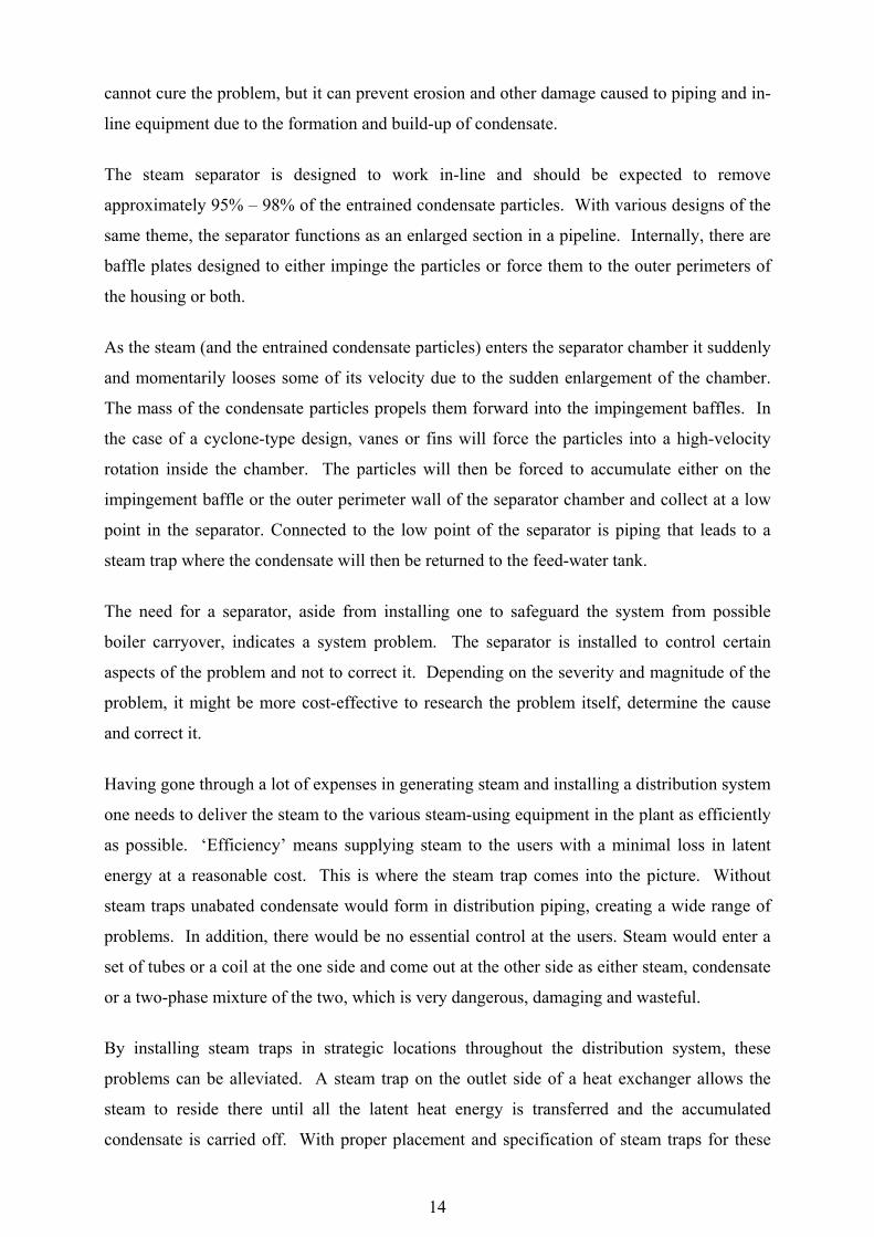
The refrigeration cycle used at Lambert’s Bay is similar to the simple vapour compression

cycle, except for the addition of a receiver and flash chamber. The following schematic

representation demonstrates this:

Pump

4

2

1

condensor

evaporator

compressor

expansion valve

QL

QH

TH

TL

Flash chamber

Figure 5: Schematic representation of ammonia refrigeration plant

The purpose of the flash chamber is to ensure that only saturated ammonia gas leaves the

chamber before entering the compressor and that the saturated liquid left behind enters the

evaporator, ensuring efficient pumping of the refrigerant.

In determining the coefficient of performance (3RNHCOP ) for the cycle shown in figures 5 and

6, the different mass flow rates through the evaporator and compressor must be known, as

well as the quality and temperatures of the ammonia at the exit of the evaporator and

compressor.

The flash chamber divides the cycle into two parts, the evaporation part and the condensing

part. Each part has a different mass flow rate, which will affect the Carnot efficiency.

( )( ) pumpg

evapinevapoutf

innet

LRNH whhm

hhmW

QCOP

+−

−==

124

4

,3 &

& (2. 6)

By using the coefficient of performance (COPR) to determine the efficiency of the

refrigeration cycle, the assumption has been made that the refrigeration cycle is an ideal

vapour-compression cycle. In the latter refrigeration cycle, the flash chamber ensures that the

compressor receives the refrigerant at saturated gas and that the evaporator receives the

refrigerator at saturated liquid. This leads to different mass flow rates at the evaporator and

21

condenser. The mass flow ratio has an effect on the 3RNHCOP for the flash chamber cycle

from a Reverse Carnot heat engine viewpoint.

The temperature-entropy diagram for a simple vapour-compression refrigeration cycle with a

flash chamber is shown below. The Reverse Carnot COP, which includes the flash chamber

effect, is set out in the following paragraph. This efficiency is the ideal efficiency of the

refrigeration cycle in place at Lambert’s Bay and provides an indication of the maximum

COPR that can be achieved.

Figure 6: T-s diagram for vapour-compression cycle with flash chamber

The thermodynamic temperature scale used is the Kelvin scale. Its derivation is shown in

Ģengel, 1994. For a Reversed Carnot cycle, the following relation holds:

Lg

Hf

L

H

L

H

QmQm

qq

TT

&

&== (2. 7)

The coefficient of performance for this cycle is:

22

1

1

,3

−==

L

Hinnet

LRNH

QQW

QCOP (2. 8)

From (2.7), the following can be derived:

Lf

Hg

L

H

TmTm

QQ

&

&= (2. 9)

and therefore, the coefficient of performance for an ideal vapour-compression refrigeration

cycle with a flash chamber is defined by:

1

13

−=

L

H

f

gRNH

TT

mmCOP

&

& (2. 10)

From the derivation (equation 2.10) it is clear that, as the ratio of gas-to-liquid mass flow rate

decreases, the coefficient of performance will increase.

To monitor the coefficient of performance, the mass flux at the outlets of the evaporator and

the compressor needs to be measured and the source and sink temperatures at equilibrium

must be measured for an accurate result. Furthermore, a central data processing point in the

factory is needed where the data is sent to a computer for further calculations. To know the

true coefficient of performance, the enthalpy of the refrigerant before and after the evaporator

and compressor, as well as the different mass fluxes, are needed. The pump’s work must also

be determined. This can be done electronically by measuring the current. However, all of

these actions require a large amount of capital to install and are therefore not implemented in

the industry.

Improving the Efficiency of the Refrigeration Cycle

By improving the energy efficiency of the different components in the refrigeration cycle, the

efficiency of the entire refrigeration cycle will increase. The refrigeration plant consists of the

following equipment: compressor, evaporator, condenser, valves and piping. The following

23

section will discuss the different components in the refrigeration cycle and how to determine

and improve their efficiency.

Compressor

A compressor is used as a means to move vapour or gas within a refrigeration system. The

adiabatic efficiency of a compressor is defined as the ratio of the work input required to raise

the pressure of a gas to a specified value in an isentropic manner to the actual work input. An

enthalpy-entropy diagram of the process will show the different paths best.

h

[kJ/kg]

1 inlet state

isentropic process

s2s=s1

P2 exit pressure

P1

2a 2s

h1

h2s h2a

actual process

wa ws

s [kJ/kgK]

Figure 7: h-s diagram of an adiabatic compressor

The adiabatic efficiency of a compressor relates the isentropic work input to the actual work

input:

a

sC w

wworkcompressoractual

workcompressorisentropic==

____η (2. 11)

By neglecting the changes in the kinetic and potential energy of the refrigerant being

compressed, the efficiency can be obtained as a relation between an isentropic compression

process enthalpy change and the actual compression process enthalpy change (figure 7):

24

12

12

hhhh

a

sC −

−≅η (2. 12)

Determining the actual inlet and outlet enthalpies of the compressor, h1 and h2a respectively, is

straightforward if the pressure and temperature is available. To find the ideal outlet enthalpy

(isentropic path), h2s, the thermodynamic property tables can be used.

Serious wear of cylinder walls and rings can result if an appreciable quantity of liquid returns

with the suction gas. Large masses of liquid can damage the valves (for reciprocating

compressors) or can cause more serious damage. Liquid returning steadily at rates too low to

cause immediate evident damage will, however, reduce cylinder lubrication and cause

extremely rapid abrasion of cylinder walls and rings. When the system has been installed

carefully and properly with no foreign matter or liquid entering the compressor, it will operate

satisfactorily for many years.

Evaporator

Losses at the evaporators can mostly be ascribed to fouling on the outside of the evaporator

fins or inside the tubes. Whatever the losses, it can be determined if the overall design heat

transfer coefficient, Udesign, is known, and if the overall actual heat transfer coefficient, Uactual,

which includes the effect of losses is known. By calculating the heat transfer to the

refrigerant or air, Q& , the overall heat transfer coefficient can be calculated from the following

equation:

( )LH TTxUPQ −Δ=& (2. 13)

Temperatures TH and TL are known and also:

( )inout hhmQ −= && (2. 14)

Therefore, in order to calculate the heat transfer rate at the evaporator, the mass flow rate

must be measured and the enthalpy at the exit and entrance of the heat exchanger must be

determined. From equation (2.14) the heat transfer rate, Q& , can be calculated and from

equation (2.13) the overall heat transfer rate, U, can be calculated.

25

Proper evaporator piping and control are necessary to keep the cooled space at the desired

temperature, as well as to adequately protect the compressor from surges of liquid ammonia

from the evaporator.

Condenser

Induced draft cooling towers use the evaporation of water to condense the superheated

refrigerant gas to a sub-cooled liquid. Fouling on the refrigeration pipes limits heat transfer to

the water or air.

Fouling in or on refrigerant pipes leads to a decreased refrigeration capacity in the evaporator

or condenser. Improving the heat transfer rate demands less work from the compressor for

the same cooling capacity.

By increasing the heat load from the refrigerated area while the compressor work input

remains constant, the coefficient of performance (COP) increases. This could be done by

improving the performance of the cooling towers, or the heat transfer from the heat

exchangers.

Oil in ammonia systems

Oil is miscible with liquid ammonia only in very small proportions. The evaporation of

ammonia increases the oil ratio, causing the oil to separate. The increased density causes the

oil to form a separate layer below the ammonia liquid, which can cover the heat transfer

surface in the evaporator, thereby reducing performance. Therefore, oil must be removed

periodically or continuously from the point where it collects. The service valves on the

compressor open and close frequently and sometimes do not seat properly. Therefore, an

additional stop valve can be used in the suction take-off to each compressor.

In addition, there should be oil separators in the discharge line of each compressor. A high-

pressure float valve drains the oil back into the compressor crankcase or oil receiver. The oil

separator should be as far as possible from the compressor to cool the discharge gas before it

enters the oil separator. Liquid ammonia must not reach the crankcase.

26

Insulation of Refrigeration Piping

Insulation between refrigeration devices should be checked for any damage. By measuring

the surface temperature of the insulation, the overall actual heat transfer coefficient for the

insulation can be calculated and compared to new insulation.

Purging of Air in Ammonia

‘Purging’ is a term used to describe the process of removing unwanted air, vapours, dirt or

moisture from the system. Air in a refrigeration system takes away some of its functioning

capacity and failure to remove such air can be costly in terms of operating efficiency and

damage to equipment. The heat transfer efficiency of any refrigeration system will greatly

improve when undesirable, non-condensable gas is removed. This process of removing air is

called purging.

No matter how hard one tries to avoid it, air will get into the system and accumulate on the

inner surface of the heat exchanger, essentially creating an insulation barrier. Air could enter

a refrigeration system through several mechanisms. When the suction pressure is lower than

atmospheric pressure, air can enter through seals and valve packing. Air can also rush in

when the system is opened for repair, coil cleaning, when equipment is added, when the

refrigerant truck is charging the system or when oil is added. This accumulated air insulates

the heat transfer surfaces and, in effect, reduces the size of the condenser. To offset this size

reduction, the system must work harder by increasing the pressure and temperature of the

refrigerant. Therefore, prompt removal of air is essential.

Before air can be removed, one must determine where it will collect. With multiple

condensers and receivers it could be difficult to determine the exact location of the air.

Condenser piping design, component arrangement and operation affect the location of air. It

is important to frequently purge each suspected air purge point (one at a time) to ensure all the

air is removed from every location.

27

Figure 8: Evaporative condenser

(Rockwell & Quake, 2001)

With an evaporative condenser (figure 8), the velocity of the entering gas prevents any

significant air accumulation upstream from point X. High velocity past point X is impossible,

because the receiver pressure is virtually the same as the pressure at point X. To ensure that

air accumulates and move into the purger, an air leg is recommended. The purge connection

on a receiver should be at the point furthest from the liquid inlet.

The easiest way to estimate the amount of air in the refrigeration system is by checking the

condenser pressure and the temperature of the refrigerant leaving the condenser. By

comparing the findings with data provided in a temperature-pressure chart, such as the one

published in the ASHRAE, 1997 Fundamentals Handbook, the extra cost caused by air

accumulation from compressor operation can be estimated. For each 27.58 kPa of excess

head pressure caused by air, the power cost to operate the compressor increases by 2% and the

compressor’s capacity is reduced by 1% (Rockwell & Quake, 2001).

Removal of Contaminants in the Refrigerant

Ammonia is a powerful solvent which removes dirt, scale, sand or moisture remaining in the

pipes, valves and fittings during installation. These substances are swept along with the

suction gas to the compressor, becoming a danger to the bearings, pistons, cylinder walls,

valves and lubrication oil.

Operating temperatures in actual cycles are established to suit the temperatures required at the

cold medium and the temperature acceptable for the heat sink. The practical temperature

gradient required to transfer heat from one fluid to another through a heat exchanger, falls in

28

the range between 5 oC and 8 oC. This leads to an increase in the work required to produce

the desired refrigeration effect, because the temperature difference has increased.

In the refrigerant cycle, the refrigerant gas is superheated at both the evaporator and the

compressor. During the evaporation process, the refrigerant is completely vaporised partway

through the evaporator. As the cool refrigerant vapour continues through the evaporator,

additional heat, which superheats the vapour, is absorbed. Pressure losses caused by friction

furthermore increase the amount of superheat. When superheating of the refrigerant occurs at

the evaporator, the enthalpy of the refrigerant is increased, additional heat is extracted and the

refrigeration effect of the evaporator is increased. No useful cooling takes place when

superheating occurs in the compressor suction piping. The increased refrigeration effect in

the evaporator is usually offset by a decrease in refrigeration effect in the compressor. This

occurs because the volumetric flow rate of a compressor is constant, and therefore the mass

flow rate and refrigeration effect are reduced by a decrease in refrigerant density caused by

superheating.

Refrigerant superheating also occurs at the compressor. Under ideal conditions, the

refrigerant enters the compressor as a saturated vapour. Increasing the pressure will increase

the temperature and cause superheating. Superheating caused by the compression process

will not improve cycle efficiency, but will result in bigger condensing equipment and large

compressor discharge piping.

De-superheating is the process of removing excess heat from the superheated refrigerant

vapour and, when accomplished through means external to the cycle, it could be beneficial to

system performance. Also, de-superheating the high-pressure refrigerant (hot gas) that leaves

the compressor, will reduce the required condenser capacity and provide a high-grade heat

source for other process uses. A typical application would be the preheating of boiler makeup

water or process water.

Liquid sub-cooling occurs when a liquid refrigerant is cooled at a constant pressure below the

liquid’s condensation temperature. When sub-cooling occurs through a heat transfer method

external to the refrigeration cycle, the refrigeration effect of the system is increased, because

the enthalpy of the sub-cooled liquid is less than the enthalpy of the saturated liquid. Sub-

cooling of the liquid upstream of the throttling device also reduces flashing in the liquid

piping. The work input is reduced and the refrigeration effect increased.

29

Hot gas bypass is a method of placing an artificial heat load on the refrigeration system in

order to produce stable suction pressures and temperatures when the refrigeration load is very

low. Bypassing hot gas from the compressor discharge to the evaporator inlet or compressor

suction produces the heat load. Although hot gas bypass permits stable compressor operation

at low load, it wastes energy.

When a refrigerant system operates with the evaporator temperature close to 0 oC or less,

freezing of the evaporator coil is inevitable. Defrosting accessories are available from the

manufacturers for systems operating under these conditions.

Cold Store Doors

A lot of energy and time is spent to produce cold air from hot humid air to temperatures

below 0 oC. The cold storage door plays an important role in today’s cold storage warehouse

and the reasons are obvious when you look at some of the conditions currently faced by

warehouse operators and owners.

Stewart (2001) wrote an article on the effect of insulated door openings in cold storage

warehouses, in which some points that affect modern cold storage doorways were put

forward. Below follows a summary of these points.

Energy costs continue to consume a significant portion of a warehouse’s operating budget.

Approximately 10% of a warehouse’s operating budget is tagged to the electricity account.

Changing product mix and customer quality demands prompted many facilities to take

temperatures below the former 0 oC benchmark. Furthermore, these temperatures had to be

held consistent through the distribution chain.

More goods are flowing through warehouses. Studies showed that approximately 46% of the

warehouses worldwide are seeing increased inventories, with approximately 42% reporting

higher inventory turnover during 1998. Facility material handling systems will have to keep

abreast with the pace. A high-density freezer store/deepfreeze cold storage warehouse is the

most expensive type of storage to operate. The solution is high-density storage in the form of

mobile racking systems to provide maximum space utilisation, access to every location (‘First

In, First Out’), least product damage, greater flexibility, a simple operating system, lowest

30

initial capital cost per useable location and greatest income potential for any given size of

building.

Faster material-handling equipment, such as powered pallet truck trailer-to-transport pallets

from road vehicle over dock leveller into the drop temperature area, cause bottlenecks through

the insulated doorway into the deepfreeze area.

It is a fact that, for productivity reasons, cold storage doors are left open. With traffic

entering and leaving the cold storage rooms, opportunities for air transfer are greater and

result in a vast amount of wasted energy. In order to take corrective action, the open doors

will have to be monitored more fully and understood better by those in charge of the

warehouse operation.

The design and location of cold storage door systems should encourage the fleet of forklifts to

move as efficiently as possible (on average, forklift drivers can spend up to 50 seconds going

through a door).

The efficient operation of any refrigeration system is faced with two problems: infiltration and

frost. The following section will discuss how infiltration and frost can result in excess, but

avoidable, costs and how cold storage doors can help one control the escalation of these costs.

A large part of the refrigeration capacity at cold stores is wasted on the freezing of water due

to an increase in the humidity contents of air when product handling requires opened doors.

The forming of frost on the evaporator surface insulate the surface and decrease the overall

heat transfer coefficient of the evaporator. This leads to inefficient heat removal in cold

stores.

The removal of moisture in cold stores is therefore an option for more energy-efficient cold

storage operation. The drying of air (removal of moisture) can be done in many ways. The

purpose is to remove moisture from air in the regions in front of the door that are most likely

to enter the cold store as the door opens. A buffer region can be formed in front of the door

by means of rubber curtains. Air is taken from just before the buffer region and the drier air is

then forced into the buffer region, causing a positive pressure and ensuring that only dry air

enters the cold stores. The drying of air with dehumidifiers can occur in two ways: absorption

dehumidifying and desiccant dehumidifying.

31

With absorption dehumidifiers, a hygroscopic salt solution (see figure 9) is pumped around

and sprayed into the dehumidifier (A). Humid air (from outside or recycled air) passes into

the dehumidifier. This air comes into close contact with the hygroscopic salt solution spray,

which absorbs the moisture present in the air. Dry air leaves the top of the unit and the salt

solution, including the absorbed moisture, collects in the lower part of the unit. By

subsequently cooling the salt solution, the air is cooled and dried simultaneously. Drip

catchers at the air outlet of the dehumidifier ensure that the air stream does not contain any

particles salt solution.

Figure 9: Principle of operation of the absorption dehumidifier

(http://www.kathabar.imtech.nl/)

To ensure a stable concentration of salt in the dehumidifier, the absorbed moisture has to be

evaporated. Therefore, a part of the (diluted) salt solution is pumped to the regenerator (B).

Here, the hygroscopic salt solution is pumped and sprayed around again. At the regeneration

side, water is evaporated by heating the salt solution. A minor secondary air stream passing

through the regenerator absorbs this moisture and takes it outside. The concentrated salt

solution returns to the dehumidifier. The process flow diagram indicates that the cold

(diluted) salt solution from the dehumidifier meets the ‘warm’ salt solution in the regenerator.

A heat exchanger, placed between these flows, will preheat the ‘cold’ solution before it enters

the regenerator. The warm solution will radiate heat, hence the cooling down before it is used

in the dehumidifier again.

Desiccant dehumidifiers utilise a ‘sorption’ material to attract and hold moisture from air.

Once the sorption material (called a desiccant) is ‘saturated’ with moisture, it can be

32

reactivated or regenerated. Reactivation is usually accomplished by thermal means and

restores the desiccant’s dehumidification capacity. The mass exchange of the moisture from

and to an air stream occurs in the vapourisation phase.

Desiccant dehumidifiers are required for use below the frost point where mechanical

refrigeration type dehumidifiers experience freezing on the coil surface or when

dehumidification is required, but cooling is not, such as for dry goods storage or preservation

requirements. Desiccant dehumidification is also utilised to provide for humidity control

independent of temperature control in occupied spaces.

Figure 10: Dessicant dehumidifier operation

(http://www.hbcotes.com/english/home.html)

Doors have to be opened and products have to be moved in and out of the cold storage space

to justify the cost of the space. In a busy facility, this occurs hundreds of times per day.

Every time the doors are opened, two air streams are set in motion at the doorway, namely

cold, dry air that escapes from the room along the floor and warm, moist air that enters

through the upper section of the door.

The warm, moist air stream almost immediately migrates to the evaporator coils to form frost.

This air infiltration can account for more than half the total refrigeration load of a cold storage

facility. The role of the evaporator coil in the refrigeration process is to draw heat and

moisture from the air, supplying cold and dry air resulting in and maintaining low

temperatures within the cold storage room. Additional units may be out in the dock-drop

temperature area to cool and dehumidify air before it enters the cold storage room and to keep

33

products cold during loading and unloading, or otherwise dehumidify and heated through

mechanical dehumidifiers.

If the product entering the room has not yet been pre-cooled, it can allow considerable

quantities of heat and moisture to enter with the warm air through the open door. The

(condensed) moisture drawn from the air accumulates on the evaporator coil and turns into

frost. As more moisture enters the cold storage room with each opening of the door, so the

frost layer grows and acts as an insulator. System efficiency therefore degrades, ultimately

causing the unit to become inoperative. When the refrigeration system or the person

responsible for operating the system detects the frost build-up, the refrigeration process is

suspended and heat must be applied to the coil to melt the frost (called the defrost cycle).

Fortunately, the full effect of this air exchange does not occur immediately as the door is

opened. The rush of the door opening, traffic going through the door and differential

pressures will initially disrupt the course of the airflow, causing the warm and cold air streams

to mix at the doorway. There are approximately 15 to 60 seconds to close the door before the

air streams reach a steady state (still air). Preventing or minimising the ability of the air

streams to reach a steady state means reducing the open door time. Based on a time study,

opening and closing a manual door for an efficiently run facility is close to 120 seconds.

Modern high-speed, horizontal-opening doors open at a speed of 1.1 meter per second.

Therefore, to open and close a door would be approximately 6 seconds.

Telltale signs of losses in temperature and financial terms are the noticeable wet floor, fog

(mist) outside the deep freeze entrance and the slippery ice on the inside caused by heavy,

cold air escaping from the deep freeze. The longer the door is open and more cold air flows

out at the bottom and creates a vacuum at the top to be filled by warm air that flows in at the

top, the more energy is lost. It is therefore essential to stem the cycle through a faster,

automatic high-speed door.

Air curtains (air knives) are also an alternative option to a door (see figure 11). Air curtains

minimise the amount of water vapour travelling from the high vapour pressure region (outside

the cold store) to the low vapour pressure region (inside the cold store). This phenomenon is

known as water vapour infiltration and increases the latent heat load of the cold stores.

Another unwanted occurrence is the formation of frost on the evaporator coils, which

obstructs the airflow through the coil and needs to be defrosted by bypassing superheated gas

34

through the evaporator coil. The air curtain limits water vapour infiltration by approximately

70% – 90% of the amount that will infiltrate without any obstruction. Applying the use of air

curtains where high vapour infiltration occurs will lead to significant energy savings.

Figure 11: Infiltration

In addition to the energy cost connected with the build-up of frost on the evaporator coils,

there is the cost of defrosting. Theoretically, defrosting would require about 50% – 100% of

the energy needed to make the frost in the first place. Conducting an energy audit for cooling

rooms are unique to each situation, but there are certain similarities. Most cold stores have

the problem of moist air entering the room and thus increasing the latent heat load inside the

room. Factors that need to be considered are the volume of the room, the surface area of the

walls and the surface finish, the heat load that needs to be removed per unit time, the surfaces

covered by frost and an approximate volume of the ice, as well as the average dry and wet-

bulb temperatures of the room. An energy balance will identify the amount of heat load

contributed by the moist air (Stewart, 2001).

2.2.6 Measuring Instrumentation

In determining the energy efficiencies of different equipment or systems, it is necessary to

determine the qualitative and the change in quantitative properties of the working fluid or

fluid under consideration. The quantitative properties are mostly mass flow and can be

obtained by measuring the volume flow rate (density must be known) or mass flow rate of the

fluid. The qualitative properties can be obtained from pressure and temperature

35

measurements. A criterion that the measuring instruments must satisfy is that the

measurements must be electronically stored to enable long-term (seasonal) monitoring.

Flow meters are used to monitor and measure volume and mass flow rates and are divided

into five basic categories, based on the method of measurement (Bagajewicz, 2001):

i. Differential pressure meters

ii. Velocity meters

iii. Positive displacement meters

iv. Mass meters

v. Variable area meters

Several factors play a role in the selection of the best flow meter for a particular application,

for instance fluid properties, desired performance, method and/or ease of installation, safety,

environmental impact and cost (often the overriding factor).

Differential pressure meters consist of three general types, namely orifice meters, venturi

meters and flow nozzles. Orifice meters are the most widely used differential pressure

meters. To maintain accuracy, they require 5 – 40 straight pipe diameters upstream of the

meter. These flow meters have many advantages, which include durability, low cost for large

pipe diameters and the ability to be used at a variety of temperatures. The disadvantages are

their high sensitivity to density and viscosity changes, and a tendency to erode. Venturi

meters are used in high flow rate applications and are more expensive than orifice meters.

However, in high flow rate applications they may cause significant pressure losses and

diminished accuracy. Flow nozzles are used when capacity is an important issue and they

work well in high-velocity, high-temperature and high-turbulence situations. Flow nozzles

are less expensive than venturis, but result in higher permanent pressure losses and are less

accurate.

Velocity meters measure fluid velocity and use the relationship AvQ ⋅= to calculate

volumetric flow rates, where Q is the volumetric flow rate, v the fluid velocity and A the flow

meter cross-sectional area. There are five basic types of velocity meters, namely

electromagnetic, vortex, turbine, ultrasonic and pitot meters. Fluids used in electromagnetic

meters must be electrically conductive and non-magnetic. Because there are no mechanical

parts that impede fluid flow, electromagnetic meters are excellent for streams containing

particles or corrosive chemicals. Other advantages include their ability to provide accurate

36

voltage signals in laminar and turbulent flow, as well as their low sensitivity to changes in

density, pressure and viscosity. A disadvantage of these meters is the potential of the

electrodes to become coated, thereby reducing errors in the reading. However, this can be

eliminated by keeping flow between 2.44 m/s and 6.05 m/s.

Mass flow meters are classified in four types, namely Coriolis, thermal, heated element and

temperature rise mass flow meters. Coriolis meters are the most accurate instruments and,

until 1999, were mainly used in critical control loops and for the management of high-valued

fluids. Advantages include their high accuracy, large flow range and tight control ability. In

addition, they do not obstruct the fluid, do not need recalibration and can be used with

different types of fluids. Thermal mass flow meters are effective with clean, low-density

gases. They are used to measure gas flow in ducts, pilot plants, purge streams and leak

testing, and are most commonly used in “dopant” gas flows for semiconductor production.

One of the advantages of a thermal mass flow meter is high accuracy. A disadvantage is the

coating of probes by dirty fluids and the need for uniform fluid flow.

Temperature measuring devices are divided into three groups:

i. Thermal expansion thermometers

ii. Electrical devices

iii. Radiation-based devices

Thermal expansion thermometers are based on the thermal expansion of either liquids or

solids. Many thermal expansion thermometers are relatively inexpensive, but they are not

very compatible with the modern computer-based data acquisition systems. Advantages are

their simplicity and their low cost. Disadvantages include that they need to be repaired at the

factory and calibration changes with handling. Electrical devices include thermocouples,

thermo resistance meters and thermistors. Of these, thermocouples are the less expensive and

more popular electrical device. A disadvantage, however, is the cold junction that may affect

calibration. Thermo resistance meters are accurate, but more expensive than thermocouples,

while thermistors can work over a very narrow span with no cold junction. A disadvantage is

their non-linear response.

Process pressure measuring devices are divided into three groups:

i. Liquid column devices

ii. Elastic element devices

37

iii. Electrical sensing devices

With liquid column devices, pressure is measured by determining the height of a liquid

column. If the density of the liquid is known, this height is a measurement of the pressure.

Most types of liquid column devices are commonly called manometers. There are three types

of elastic element pressure measuring devices, namely Bourdon-tube, bellows and diaphragm

elements. These devices rely on the deformation of an elastic material that is proportional to

the applied pressure. Electrical sensing devices operate on the property that electrical

resistance of conducting solids changes with diameter and length.

Monitoring and analysing energy consumption of different equipment and systems at once

over a certain period require effective and fast conveying of measurement signals to

processor. This requires the measurement signals to be conveyed electronically. Devices

performing this operation are called transducers. Ideal transducers are linear, but in practice

they are affected by zero offsets, hysteresis, et cetera. By using transducers the measurement

can be transformed into an electronic signal and sent to a processor where the data is

processed.

38

3 LAMBERT’S BAY ENERGY ANALYSIS

3.1 Energy Analysis Strategy

The energy analysis that was carried out consisted of a walkthrough audit, an energy

consumption analysis, an energy efficiency analysis, an energy efficiency upgrading analysis

and a payback period calculation. An energy efficiency study was implemented at Lambert’s

Bay Foods with minor adjustments to adapt to Lambert’s Bay’s circumstances and financial

limitations. Therefore, this study focused on identifying losses and suggesting solutions to

minimise the losses in order to improve the thermal efficiency of the processes or equipment.

3.2 Plant Layout

The plant comprises a French fries production line, three cold stores, a blast freezer, a

compressor room, a loading bay and a boiler room. All the abovementioned is shown on the

schematic drawing in figure 12, except the boiler room, which is situated approximately 30 m

from the production line in another building adjacent to the French fries production line.

Figure 12: Schematic representation of plant layout

39

3.3 Walkthrough Audit

A walkthrough audit checklist was generated from a checklist suggested by Kreith and West

(1997) – see appendix A.4. In June 2001, a walkthrough audit of the premises was conducted

to identify energy wastages and possibilities of energy efficiency improvements (see appendix

A.4).

Visible signs of energy wastages in the form of ice were found on the uninsulated fittings of

the refrigeration pipe network, as well as on the uninsulated valves and similar items of the

refrigeration system inside the refrigeration room. Calculations were conducted to estimate

energy losses on the refrigeration pipes.

Steam leaks were also detected at various locations in the plant. Visible steam losses are at

the steam peeler, the valve near the hot water reservoir and at the blanchers. In the case of the

steam peeler, the same situation occurred at a French fries plant in the Netherlands (Dutch

National Team, 2000). There, the discharge steam was recovered by means of a heat

exchanger.

Huge potential for energy savings exists by modifying the production line. By increasing the

production line efficiency, less energy is wasted by adding value to defective products that are

thrown away. A large amount of refrigeration energy is wasted at the flow freezer, where the

frozen French fries are manually sorted and exposed to a warm environment (a human being

requires a comfortable working environment). The temperature increase caused by the

exposed fries needs to be corrected by putting the packed fries into a blast freezer, rapidly

cooling the fries to –37 oC. An optical sorter can be used to shorten the length of exposure of

fries to the warm environment (temperatures close to 0 oC). Automating the handling of

material from the packing line to the cold stores means that the environment in which the fries

are packed and transported can operate at a much lower temperature. This, however, requires

a thorough feasibility study to motivate the capital needed for such procedures.

40

3.4 Energy Consumption

In order to determine the feasibility of an energy analysis, knowledge of the main energy-

consuming equipment or processes is essential. Energy accounts for six months (December

2001 to May 2002) were used to compare the main energy-consuming equipment (see

appendix A.1). By using an average price for electricity, assuming the plant operates 24

hours a day, coal and electricity consumption can be compared on a cost basis. From the

obtained accounts, coal is accountable for 79% and electricity for 21% of the total energy

costs. The energy cost for coal per joule is R0.0157 and for electricity R0.0446. The

different steam users are indicated in figure 13, with its fraction of total steam consumption

(data obtained from Uticon-Dynatherm Industrie bv, 1994).

Figure 13: Pie chart indicating the main steam users

The largest steam user is the large dryer, which consumes 33% of the total steam

consumption. The fryer consumes 16% of the total steam production to fry the cooked fries.

Other large steam consumers are blanchers 1, 2 and 3 (10%, 4% and 3% of total steam

production respectively), the small dryer (15%) and the steam peeler (9%).

The electricity usage can also be compared in terms of equipment and is indicated in the pie

chart below.

41

Figure 14: Electricity consumption of various users

From figure 14, it can be seen that refrigeration contributes 67% (FES compressor, M&M

compressors 2, 3 and 4, refrigeration pumps, air compressors, condensor fans and pumps) of

the total electricity consumption, which makes it the largest user of electricity. The

consumers of refrigeration energy can furthermore be divided into different equipment.

The data from the above figures was used to draw up a Sankey diagram (figure 15) to indicate

the energy flow graphically.

42

Figure 15: Sankey diagram of total energy flow in plant

From the Sankey diagram, the dryers and blanchers are the largest users of energy and then

the compressors and fryer follow. The Sankey diagram graphically helps to establish focus

areas in an energy efficiency analysis.

3.5 Economic Decision Analysis Approach

Where the payback period is so long that inflation needs to be considered, an actual Rand

approach will be used. Assumptions made to simplify the economic analysis were a constant

interest rate and, that for short payback periods (less than five years) the inflation effect is

insignificant, therefore, the payback amount will be the energy savings that were achieved.

Other costs, such as maintenance, will be included in the overall cost of the equipment where

possible. Fabrycky, Thuesen and Verma (1998) offer the following formula which relates the

present value, single payment per interest period and the number of interest periods:

43

( )( )( )n

n

iiiAP

+⋅−+⋅

=1

11 (3. 1)

After manipulation, the number of interest periods (which, in our case, will be monthly) can

be calculated:

( )i

iAP

n+

⎟⎟⎟⎟

⎠

⎞

⎜⎜⎜⎜

⎝

⎛

⋅−=

1ln

1

1ln

(3. 2)

In most cost analyses in this document n is the number of months, P the initial capital outlay

and A the monthly energy savings.

44

3.6 Steam

3.6.1 Dryers

The dryers, which consume 48% of the total steam production, were analysed to measure their

performance. The function of the dryers is to control the moisture content of the fries. This is

achieved by removing moisture from the fries by blowing warm, dry air through the fries as

they are transported on a chain conveyor belt. Air is sucked in (by centrifugal fans) from

outside the plant and heated with steam-to-air heat exchangers to decrease the relative

humidity of the air. The air moves from right to left through the dryers as shown in figure 16

and the fries move on the chain belt in the opposite direction. The low relative humidity of

the air improves the mass transfer potential of moisture from the fries into the air.

Figure 16: Schematic drawing of dryer illustrating airflow

Measurements of the surface temperature of the fries and the wet and dry-bulb temperatures

of the air in each section of the dryer were taken (appendix J.1) in order to calculate the

relative humidity of the air inside the dryers. The relative humidity difference between the air

and the moisture just above the surface of the fries is the driving force for evaporation. It was

found that one of the steam-to-air heat exchangers in the dryer was performing inadequately,

which limited the current capacity of the dryer and prohibited an increase in production rate.

45

Figure 17: Dry and wet-bulb temperatures of each section

As indicated in figure 17, the outside air is at a relative low dry and wet-bulb temperature. As

soon as the air moves through the first heat exchanger, the dry-bulb temperature is supposed

to increase and the wet-bulb temperature is supposed to stay constant. However, it was found

that the wet-bulb temperature increased with the dry-bulb temperature and that there was no

airflow through the first heat exchanger. Further investigation showed that air from the plant

is sucked in from the right side of the dryer between the belt and the opening. This action

prohibits the first heat exchanger from being fully utilised, thereby limiting production

increases and leading to inefficient use of centrifugal fans.

Figure 18: Specific humidity of air through each section

Figure 18 indicates the specific humidity of air at different sections in the dryers. This is an

direct indication of the amount of humidity in the air which must increase right through the

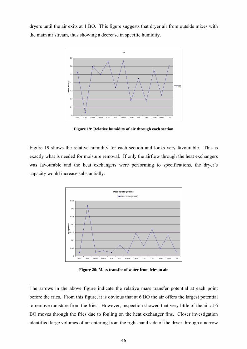
46

dryers until the air exits at 1 BO. This figure suggests that dryer air from outside mixes with

the main air stream, thus showing a decrease in specific humidity.

Figure 19: Relative humidity of air through each section

Figure 19 shows the relative humidity for each section and looks very favourable. This is

exactly what is needed for moisture removal. If only the airflow through the heat exchangers

was favourable and the heat exchangers were performing to specifications, the dryer’s

capacity would increase substantially.

Figure 20: Mass transfer of water from fries to air

The arrows in the above figure indicate the relative mass transfer potential at each point

before the fries. From this figure, it is obvious that at 6 BO the air offers the largest potential

to remove moisture from the fries. However, inspection showed that very little of the air at 6

BO moves through the fries due to fouling on the heat exchanger fins. Closer investigation

identified large volumes of air entering from the right-hand side of the dryer through a narrow

47

opening where the fries chain belt exits. This occurs, because the pressure difference required

for the air to move from 6 BO to 6 ONDER is much higher than for the air to travel from the

outside of the plant to 6 ONDER. Another possibility is that the channel through which air

moves from the outside to 6 BO is blocked. Either way, it is advisable that the channel, as

well as the heat exchanger, is inspected and cleaned on a regular basis and that the pressure

difference needed for airflow through the conveyor opening is increased. The latter can be

achieved by adding an additional channel and obstruction section over the conveyor. Figures

18 to 20 were obtained through spreadsheet calculations in appendix J.2.

Calculations to Estimate Specific Humidity and Mass Transfer

Calculations to determine the specific humidity from the dry and wet-bulb temperatures in

figure 17 were carried out in an Excel spreadsheet (appendix J.2). For determining the

specific humidity, one looks at an adiabatic saturation process where the incoming air is at

given dry and wet-bulb temperatures and the outlet air is saturated at a dry-bulb temperature

equal to the inlet wet-bulb temperature.

Tdb1 Tnb1 ω1 φ1

m1

Tdb2 = Tnb1 Tnb2 = Tnb1 ω2 φ2 = 100% m2

Tf mf hf

Figure 21: Adiabatic saturation of air

In the schematic illustration in figure 21 air at known dry and wet-bulb temperatures is

saturated by adding water spray into the air. Air enters at Tdb1, Tnb1 with a mass flow rate of

m1, water is sprayed at a temperature of Tnb1 and a flow rate of mf and it exits at Tdb2 = Tnb1,

Tnb2 = Tnb1 and a total mass flow rate of m2. The mass flow rate of dry air remains constant at

ma. From the conservation of mass for water vapour we have:

afa mmm ⋅=+⋅ 21 ωω (3. 3)

48

In equation 3.3, ma is known, but the rest are all unknown. The saturated vapour pressure at

the exit can be calculated for the wet-bulb temperature, Tnb1, from Kröger (1998):

2102

zgP = (3. 4)

where z2 is a function of the wet-bulb temperature:

786118.2110102873.4

1011050474.1

)16.273log(02808.5)16.2731(79586.10

)16.2731(76955.44

)116.273

(29692.84

112

1

1

+⎥⎥⎦

⎤

⎢⎢⎣

⎡−⋅⋅+

⎥⎥⎦

⎤

⎢⎢⎣

⎡−⋅⋅+

⋅+−⋅=

−⋅−

−⋅−−

nb

nb

TK

KT

nbnb TK

TKz

(3. 5)

With Pg2 known and the relative humidity φ2 = 1, the specific humidity at the exit can be

obtained from:

2

222

622.0

g

g

PPP

−

⋅⋅=

φω (3. 6)

where P is atmospheric pressure. From the conservation of energy:

( )222111 )( vaaffvaa hhmhmhhm ⋅+=⋅+⋅+⋅ ωω (3. 7)

Through manipulation the specific humidity at the inlet is:

( )fv

fvaa

hhhhhh

−

−⋅+−=

1

22121

ωω (3. 8)

The specific enthalpy of dry air (approximated air as an ideal gas), ha, can be obtained as

follows:

( )KTch dbpaa 16.273−⋅= (3. 9)

49

where the specific heat capacity of dry air, cpa, is correlated with a third-order polynomial

obtained in Excel:

( )( ) ( )3724

13

10705209.210083814.7

10161783.310045356.1

dbdb

dbpa

TT

Tc

⋅⋅−⋅⋅+

⋅⋅−⋅=−−

−

(3. 10)

From equations (3.9) and (3.10), the specific enthalpy for dry air at the inlet and outlet can be

calculated. The specific enthalpy for water vapour, hv, is given by the following:

( )KTcih dbpvfgwov 16.273−⋅+= (3. 11)

where the latent heat, ifgwo, is evaluated at 273.15 K and ifgwo = 2.5016x106 J/kg. The specific

heat of water vapour is given by:

( )( ) ( )613510

3

1091332.51046784.2

31334.2103605.1

dbdb

dbpv

TT

Tc

⋅⋅+⋅⋅−

⋅+⋅=−−

(3. 12)

To solve equation (3.8), the only value that needs to be calculated is the specific enthalpy of

the water liquid that is added to the incoming air, hf:

( ) PKTch fnbpwf ⋅+−⋅= υ16.273 (3. 13)

where the pressure, P, is assumed to be at atmospheric pressure at sea level and the specific

heat of water liquid is given by:

( )( ) ( )61322

3

1017582.21011283.5

108067.21015599.8

nbnb

nbpw

TT

Tc

⋅⋅−⋅⋅+

⋅⋅−⋅=−−

(3. 14)

and the specific volume:

( )( ) ( )62029

63

1090321.11009782.7

107164.31049343.1

nbnb

nbf

TT

T

⋅⋅−⋅⋅+

⋅⋅−⋅=−−

−−υ (3. 15)

50

From equations (3.13) to (3.15), the specific enthalpy of the water can be calculated and

equation (3.8) can be solved.

In order to calculate the mass transfer of water vapour into the air stream, a semi-empirical

equation proposed by Gilliland (Kröger, 1998) was used for calculating the diffusion

coefficient:

( )2333.0333.0

5.0

5.1

11

04357.0ba

badb

VVP

MMTD

+⋅

⎟⎟⎠

⎞⎜⎜⎝

⎛+

⋅⋅= (3. 16)

where Va and Vb are the molecular volume of gases a and b, which in this case is air and

water, and thus, for air Va = 29.9 and for water vapour Vv = 18.8. The molecular masses for

air and water are Ma = 28.97 and Mv = 18.016 respectively.

Assuming that the evaporation process of air blown through fries can be approached as the

evaporation of liquid inside a circular column, with air blown through it and diameter, d,

Gilliland (Kröger, 1998) supplied the following semi-empirical equation:

44.083.0Re023.0 ScD

dhSh D ⋅⋅=

⋅= (3. 17)

valid for 2000 < Re < 35000 and 0.6 < Sc < 2.5. The Schmidt number is given by:

DSc

⋅=

ρμ (3. 18)

and the Reynolds number is given by:

μμρ dGdV ⋅

=⋅⋅

=Re (3. 19)

and the mass flux, G, is given by:

51

columns

air

columns

air

AAV

Am

G⋅⋅

==ρ

(3. 20)

To solve equation (3.17), equations (3.16) to (3.20) were set into equation (3.17). The

relation between the area of the fries and the flow-through area of the columns between the

fries was approximated as Aair/Acolumns = 20/1 and the diameter of the columns through the

fries approximated as d = 0.003 m:

56.083.039.0

742.0 DVhD ⋅⋅⎟⎟⎠

⎞⎜⎜⎝

⎛⋅=

μρ (3. 21)

The mass transfer coefficient is:

( ) ( ) ( )⎥⎥⎦

⎤

⎢⎢⎣

⎡

+−

+⋅⋅

−⋅⋅

=622.0622.0 ω

ωω

ωωω dbsatf

sat

satv

Dd TTR

Phh (3. 22)

From equation (3.22), it is possible to calculate the mass transfer rate:

( )ωω −⋅⋅= satdw Ahm (3. 23)

Figures 18 to 20 were generated from the equations above. The calculations were done in

Excel (see appendix J.2).

3.6.2 Boiler

Boiler energy losses which occur are radiation losses, exhaust gas losses, poor boiler

management and combustion inefficiencies (these include oil burner inefficiencies and non-

stoichiometric combustion). Boiler efficiency can be improved through improved

combustion, flash-steam heat recovery, flue-gas heat recapturing (recuperator and

economiser) and improved TDS (Total Dissolved Solids) management. Currently, Lambert’s

Bay has a coal-fire tube boiler with a steam flow rate of 10 ton per hour (10 000 kg/h) and a

design steam pressure of 22 bar (2.2 MPa). The boiler lacks an economiser, automatic TDS

52

control, separator or superheating of steam, preheating of air and blow-down heat recovery.

The addition of these features will be discussed in the following section.

Economisers reduce the heat in the flue gas and transfer it to the boiler feed water. They can

increase the efficiency of boilers by 3% – 5% (Dutch National Team, 2001). Oxygen trim

controllers control the fuel-to-air ratio within optimal limits. An oxygen trim control system

will correct the airflow so that the combustion efficiency remains as high as possible. It can

improve boiler efficiency by 1% – 2%. Blow-down heat recovery (recovers heat and water

from TDS blow-down) recovers the flash steam resulting from boiler blow-down to a lower

pressure. Steam boilers need to be blown down in order to control the TDS level in the boiler

water between acceptable limits. This is best achieved by using a TDS control system, which

will open a valve to allow boiler water to discharge when the TDS level rises above a pre-set

limit. Relatively low TDS feed water then replaces the discharged boiler water (up to 80% of

the heat in the discharge is recoverable by using properly designed flash vessels and heat

exchangers). Due to the abnormally high TDS levels (between 700 ppm and 1100 ppm) for

Lambert’s Bay’s municipal water, this document will look at energy savings through flash-

steam heat recovery.

Flash-steam Heat Recovery

Flash steam is released from the hot blow-down water when the pressure drops as shown in

figure 22. This mixture of flash steam and blow-down water is allowed to separate in a flash

vessel (the design of the flash vessel ensures that flow velocities are low for promoting good

separation). The dry flash steam is then introduced at low pressure to the feed-water storage

tank through the steam distributor or flash condensing deaerator head. A float trap fitted to

the outlet of the flash vessel drains the residual blow-down. From the float trap, the residual

blow-down water is allowed to pass into the heat exchanger, where it gives up its heat to

circulating cold make-up water. The cooled blow-down water then flows safely to the drain.

To save energy, the circulating pump is only activated by a thermostat mounted on the blow-

down water inlet to the heat exchanger. Therefore, it will only run when blow-down water is

flowing.

53

Figure 22: Flash-steam heat recovery system with plate heat exchanger

TDS levels for boilers need to be less than 2500 ppm to 3000 ppm. Through better treatment

of the feed water, TDS levels can be decreased, thus leading to less blow-down.

Assuming a relatively constant boiler blow-down rate when operating at maximum demand

with the feed-water TDS level at 700 ppm and the boiler TDS level at 3000 ppm, the blow-

down rate can be calculated:

boilerbdfwfw ppmmppmm ⋅=⋅ && (3. 24)

where mfw is the feed-water flow rate. The feed-water flow rate is 10 000 kg/h and thus the

blow-down rate can be calculated:

fwboiler

fwbd m

ppmppm

m && ⋅= (3. 25)

The percentage of flash steam recovered in the flash vessel can be calculated through an

energy balance, assuming that the blow-down condensate flashes off to 0.2 MPa (2 bar guage,

3 bar absolute pressure):

( )

bdbarfbarg

barfbarfflash

barfflashbdbargflashbarfbd

mhhhh

m

hmmhmhm

&&

&&&&

⋅−

−=

⋅−+⋅=⋅

33

323

3323

(3. 26)

54

Thus, the rate of energy recovered by flash-steam heat recovery is:

bargflashflashrec hmE 3⋅= && (3. 27)

By substituting flashm& into the above equation and replacing bdm& , the recovered flash steam

is:

bargfwboiler

fw

barfbarg

barfbarfflashrec hm

ppmppm

hhhh

E 333

323 ⋅⋅⋅−

−= && (3. 28)

Substituting the variables in the above equation:

kWE

kgkJskgppmppm

kgkJkgkJkgkJkgkJE

flashrec

flashrec

310

/3.2725/7778.23000700

/47.561/3.2725/47.561/614.941

=

⋅⋅⋅−−

=

&

&

(3. 29)

This figure of 310 kW is obtained without further heat recovery of the condensate. The flash

steam that is recovered also leads to an improved TDS value and less oxygen in the feed

water. The equipment necessary to obtain these savings amount to R44 206,00 (Spirax-Sarco

quote reference nr. NL5287S). The monthly energy savings for the flash heat recovery

system is given by:

flashrecmonthcoalconversion

coalavailSM Et

CalCE &⋅⋅⋅

⋅=

ηη (3. 30)

With the availability ηavail = 0.97, the conversion efficiency from coal to steam ηconversion =

0.85, the calorific value of coal Calcoal = 27 MJ/kg, the cost of coal Ccoal = R400/ton, and the

time in a month, tmonth = 2.628 x 106 s, the energy savings per month are:

55

24.13773RESM = (3. 31)

The payback period is given by equation (3.2), with P the cost of system and A the monthly

energy savings:

( )i

iAP

n+

⎟⎟⎟⎟

⎠

⎞

⎜⎜⎜⎜

⎝

⎛

⋅−=

1ln

1

1ln

(3. 32)

Working with an average interest rate of 17% per annum (1.41667% per month), the payback

period can be calculated:

( ) 308.30141667.01ln

0141667.024.13773

442061

1ln

=+

⎟⎟⎟⎟

⎠

⎞

⎜⎜⎜⎜

⎝

⎛

⋅−=n months (3. 33)

Thus, the flash-steam heat recovery system as proposed above has a payback period of 3.3

months. In calculating the payback period, the installation cost and extra maintenance cost

were ignored.

3.6.3 Utilisation of Reject Steam at Steam Peeler

The steam peeler’s function is to remove the potato skin at the required flow rate. The steam

peeler removes the skin of the potatoes by means of a rapid pressure release on the raw

potatoes. This steam-potato mixture is then freely ejected into the atmosphere, where it is

separated in a deceleration duct and the steam goes upward and the skin slurry into bins which

are discarded. Figure 23 illustrates the expanded steam from the steam peeler that condenses

in the atmosphere without any recapturing of energy.

56

Figure 23: Rejected steam of steam peeler into atmosphere

Description and Mechanism of Steam Peeler

The steam peeler consists of a peeling vessel and a weighing hopper, which weighs a specific

amount of product with each batch of potatoes. When the product has entered the steam

peeler, the peeling vessel cover closes and steam is supplied through the central steam

distribution grill into the vessel at approximately 1.6 MPa (16 bar) absolute pressure. The

steam is equally divided and mixed through the product. The Dutch company Uticon-

Dynatherm Industrie bv estimates that 14% of a potato’s volume is lost in a steam-peeling

action in their energy calculations for the Lambert’s Bay Canning company. It will be a safe

approximation to assume that 14% of the potatoes’ volume that is lost contributes to the same

volume of steam being lost for any further heat recovery. A certain amount of condensate is

lost for further use and a small amount of energy is used as sensible heat added to the

potatoes, but these can all be assumed to be negligible compared to the volume of steam

assumed to be lost for any further heat recovery. To estimate the mass flow rate of the

product at different stages on the production line, a percentage loss diagram is shown for each

subsystem in the production line (table 3.1). These values were obtained from the feasibility

study Uticon-Dynatherm Industrie bv did before erecting the plant. Calculations were done

for a final product output of 100 ton per day with an availability of 0.97. Thus, the mass flow

of the final product out:

hkgm outproduct /5.429597.024

1000100, =

⋅⋅

=& (3. 34)

57

Mass flow % loss of total input Process % loss at process 9406.637 100.0% Input 9406.637 100.0% Peeling 14.003% 8089.426 86.0% Cutting/sorting/grading 15.044% 6872.453 73.1% Blanching 2.083% 6729.299 71.5% Drying 24.890% 5054.377 53.7% Frying 12.465% 4424.349 47.0% Defatting 0.971% 4381.388 46.6% Cooling and freezing 0.980% 4338.451 46.1% Packing 0.990% 4295.5 45.7% Output

Table 3. 1: Percentage loss of product mass

For a production rate of 1 000 kg/h of raw potatoes at the steam peeler, 100 kg/h of saturated

steam at 1.6 MPa (16 bar) absolute pressure is required (Uticon-Dynatherm Industrie bv,

1994). The enthalpy of saturated steam at 16 bar is 2793.88 kJ/kg (Çengel & Boles, 1994).

With an availability of 0.97 and a daily production rate of 100 000 kg/day, the total amount of

steam that enters the steam peeler is:

outproductoutproductinsteam mmm ,,, 21882.0%7.45

%0.1001.0&&& ⋅=⋅

⋅= (3. 35)

The amount of energy in the steam that enters the steam peeler is:

barginsteaminsteam hmE 16,,, ⋅= && (3. 36)

Figure 24 below shows the energy flow during one full cycle of the steam peeler.

14% of potato volume

Esteam,out

Esteam,in

Eproduct,in

Eproduct,out

Figure 24: Steam peeler energy flow

58

The steam energy available for utilisation is:

outproductinproductinsteamoutsteam EEEE ,,,,&&&& −+= (3. 37)

where the energy added to the raw potatoes is approximated as the volume of steam required

to equal 14% of the total potato. The amount of steam is then:

bargpotato

potato

barg

potatolosssteamloss v

mv

Vm

16,16,

,,

14.0⋅

⋅==

ρ&&

& (3. 38)

where the potato density, ρpotato, is 1075 kg/m3 (Garrote, Silva & Bertone, 2000) and the mass

flow of the potato is taken as 100 ton per day with an availability of 0.97, and the specific

volume of steam at 1.6 MPa (16 bar) absolute pressure, vg,16bar, is 0.124458 m3/kg (Çengel &

Boles, 1994). The energy flow rate of the steam that is wasted is then:

( )

kW

hm

hmmE

bargoutproductbargpotato

bargsteamlossinsteamoutsteam

64.700

14.021882.0 16,,16,

16,,,,

∴=

⋅⋅⎟⎟⎠

⎞⎜⎜⎝

⎛

⋅−∴=

⋅−=

&

&&&

υρ (3. 39)

Thus, for an output of 4295.5 kg/h of French fries, 700.64 kW energy in the form of steam is

discarded into the environment. With the assumption that the pressure inside the vessel is

approximately 1.6 MPa (16 bar) absolute pressure, and at saturation, this energy could be used

as an energy source for the hot water system and the defrosting system, and the rest could be

used as energy to preheat fresh water for the blanchers. Or, to minimise capital expenditure

all of the heat can be used to preheat the fresh water for the blanchers. The schematic

representation in figure 25 shows the current situation at the steam peeler.

59

Figure 25: Schematic representation of steam peeler current operation

A concept proposal (see figure 26) for the utilisation of the waste steam was developed and

payback periods were calculated for different heat exchangers. In this concept, the flash

chamber was discarded and a protection plate was placed on the inside of the deceleration

duct. This concept makes use of a finned-tube heat exchanger that transfers heat to the

process water of the blanchers.

Figure 26: Steam peeler with shell-tube heat exchanger

60

Energy Transfer Analysis of Finned-tube Heat Exchanger

A computer program was written, using Microsoft Visual Basic V.6 to evaluate a finned tube

configuration for the utilisation of reject steam (appendix K). A control volume was set up

and heat transfer and pressure drop calculations were done for the control volume (see figure

below for the control volume boundaries).

Twin mw hwin

Twout hwout deltaPw

Tsout mseout mscond hsout deltaPs

Tsin mse hsin

dx

TFin

tw

do dFin

Figure 27: Control volume for finned tube

The overall heat transfer coefficient, Uo, is based on the outside surface of the tube and was

determined for the control volume in order to determine the increase of the water enthalpy and

the decrease of the steam enthalpy. The overall heat transfer coefficient is given by the

following equation (Kröger, 1998):

1

12

ln−

⎥⎥⎥⎥⎥

⎦

⎤

⎢⎢⎢⎢⎢

⎣

⎡

⋅+

⋅⋅⋅

⎟⎟⎠

⎞⎜⎜⎝

⎛⋅

+⋅

=fo

i

oo

ii

oo ehLk

rr

A

hAA

Uπ

(3. 40)

where Ao and Ai is the respective outside and inside surface areas, hi the inner convective heat

transfer coefficient – in this case for the water, ro and ri the respective outer and inner radii of

61

the tube, k the thermal conductivity of the tube material, L the length of the control volume

considered – in this case dx, ho the outside convective heat transfer coefficient and ef the fin

effectiveness.

The outside convective heat transfer coefficient for the steam was calculated at Tsin, the steam

temperature. Correlations (see appendix K.3) obtained in Excel for the density, ρs, kinematic

viscosity, υs, conduction coefficient, ks, and the Prandtl number, Prs, for the steam were set

up in the heat exchanger program code. The abovementioned properties were obtained from

Schmidt (1969).

The Reynolds number is given by:

υρ ⋅⋅⋅

=frs

oseds A

dmRe (3. 41)

with mse the mass flow of the steam for each element and Afr the frontal area perpendicular to

the steam flow. The average Nusselt number for Pr > 0.5 is given by the correlation

suggested by Churchill and Bernstein (Mills, 1995). For Reds < 10 000 the Nusselt number is:

( )[ ] 4/13/2

3/12/1

Pr/4.01

PrRe62.03.0

+

⋅⋅+= ds

dsNu (3. 42)

and for 10 000 < Reds < 4 x 105:

( )[ ] ⎥⎥⎦

⎤

⎢⎢⎣

⎡⎟⎠

⎞⎜⎝

⎛+⋅+

⋅⋅+=

2/1

4/13/2

3/12/1

282000Re

1Pr/4.01

PrRe62.03.0 dsds

dsNu (3. 43)

and for 4 x 105 < Reds < 5 x 106:

( )[ ]5/48/5

4/13/2

3/12/1

282000Re

1Pr/4.01

PrRe62.03.0

⎥⎥⎦

⎤

⎢⎢⎣

⎡⎟⎠

⎞⎜⎝

⎛+⋅+

⋅⋅+= dsds

dsNu (3. 44)

With the Nusselt number known, the outside convective heat transfer coefficient for the

steam, hcs, can be calculated:

62

dso

scs Nu

dk

h ⋅⎟⎟⎠

⎞⎜⎜⎝

⎛= (3. 45)

For the calculation of the convective heat transfer coefficient for the water, the same approach

was followed. Correlations were set up in Excel for the density, ρw, kinematic viscosity, υw,

conduction coefficient, kw, and the Prandtl number, Prw, of the water (see appendix K.3). The

Reynolds number for the water side is given by:

wdiw

iwdw A

dmυρ ⋅⋅

⋅=Re (3. 46)

For turbulent flow, the wall friction is needed in order to calculate the convective heat transfer

coefficient for the water. The friction factor for a smooth wall from Petukhov’s formula

(Mills, 1995) is:

( ) 264.1Reln790.0 −−⋅= dwf (3. 47)

For Redw < 3000, the flow is laminar and the Nusselt number is given by:

364.4=dwNu (3. 48)

For 3000 < Redw < 10 000, Gnielinski’s formula is recommended (Mills, 1995):

( ) ( )( ) ( )1Pr8/7.121

Pr1000Re8/3/22/1 −⋅⋅+

⋅−⋅=

ff

Nu wdwdw (3. 49)

For Redw > 10 000, a simple power law formula is used:

4.08.0 PrRe023.0 ⋅⋅= dwdwNu (3. 50)

From the above correlations, the convective heat transfer coefficient for the water is

calculated as follows:

63

dwi

wcw Nu

dk

h ⋅⎟⎟⎠

⎞⎜⎜⎝

⎛= (3. 51)

The fin effectiveness is represented by the following equation (Kröger, 1998):

( )2/

2/tanh

finofin

finofinfin db

dbφ

φη

⋅⋅

⋅⋅= (3. 52)

where the above gives the fin efficiency with:

2finfin

csfin kt

hb

⋅= (3. 53)

and

⎟⎟⎠

⎞⎜⎜⎝

⎛⎟⎟⎠

⎞⎜⎜⎝

⎛⋅+⋅⎟

⎟⎠

⎞⎜⎜⎝

⎛−=

fin

fin

fin

finfin r

rrr

1

2

1

2 ln35.011φ (3. 54)

where r2fin and r1fin is the outer and inner radii of the annular fin. To calculate the hyperbolic

tan in the program, the mathematical relations below were used. The hyperbolic tan of any

function z is given by (Greenberg, 1998):

( ) ( )( )

( )

( ) z

z

zz

zz

eez

eeeez

zzz

2

2

11tanh

tanh

coshsinhtanh

−

−

−

−

+−

=

+−

=

=

(3. 55)

where e-2z is approximated by the first six terms in the following Taylor series (Greenberg,

1998):

( ) ( ) ( ) ( ) ( )!5

2!4

2!3

2!2

2215432

2 zzzzze z −+

−+

−+

−+−+=− (3. 56)

64

where 2/finofin dbz φ⋅⋅= .

The fin effectiveness can now be calculated:

( )total

finfinfin A

Ae

⋅−−=

η11 (3. 57)

where Afin is the outside fin area and Atotal is the total outside fin and tube area. With the

abovementioned calculated for the control volume, the outlet enthalpies for the steam and

water, Hsout and Hwout, can be calculated:

cvwinwout

cvsout

QHH

QHH

Δ+=

Δ−= sin

(3. 58)

The enthalpy values of steam and water were obtained from Schmidt (1969) and are

approximated by the following linear equations respectively:

( ) ( )41904019356003.1986 ⋅++⋅⋅∴=

⋅+⋅=

scss

fsscsss

mTm

hmhmH (3. 59)

( )11430001.4185 +⋅⋅=⋅= wwwww TmhmH (3. 60)

65

The unit for Hs and Hw is Watt, and ms and mw are the steam and water mass flow rates

respectively, msc is the condensate mass flow rate and hfs the enthalpy of saturated liquid

water at 1 atm pressure. Condensation will start at 373.15 K (100 oC) and from there the

steam flow rate will decrease with the condensate flow rate given by:

fgs

cvsc h

Qm

Δ= (3. 61)

with hfgs the specific enthalpy of evaporation at 1 atm absolute pressure and Qcv the heat

transfer to the water. Although the pressure in the heat exchanger will be slightly higher than

atmospheric, the steam can be regarded as if it is at atmospheric pressure.

For the pressure drop on the outside of the tubes, Zukauskus (Mills, 1995) recommends the

following:

fV

NPs ⋅⎟⎟⎠

⎞⎜⎜⎝

⎛ ⋅⋅⋅=Δ

2

2maxρ

χ (3. 62)

where the friction factor f and correction factor χ are calculated for the worst conditions in the

heat exchanger and N is the number of tube banks. The transverse pitch, ST, is 0.05 m and the

longitudinal pitch, SL, is 0.08 m. With an outside tube diameter of 0.025 m, the dimensionless

transverse pitch, PT, and the dimensionless longitudinal pitch, PL, are (Mills, 1995):

625.02.3

2

=====

LT

LL

TT

PPdSPdSP

(3. 63)

Vmax is the maximum velocity in the tube bank and for an aligned bank, the maximum velocity

occurs between adjacent tubes of a transverse row:

DSS

VVT

To −

⋅=max (3. 64)

66

The pressure drop inside the water tubes was calculated for a tube with a relative roughness

factor of ε/d = 0.00006. For ε/d > 10-4, Haaland (Kröger, 1998) recommends the following

equation for the friction factor:

211.1

10ln

75.3/

Re9.6ln

3086.0

−

⎟⎟⎟⎟⎟⎟

⎠

⎞

⎜⎜⎜⎜⎜⎜

⎝

⎛⎟⎟⎠

⎞⎜⎜⎝

⎛⎟⎠⎞

⎜⎝⎛+

⋅=

d

fw

w

ε

(3. 65)

and for a very small relative roughness, ε/d, the friction factor is given by:

2

33.33

10ln

75.3/

Re7.7ln

7778.2

−

⎟⎟⎟⎟⎟⎟

⎠

⎞

⎜⎜⎜⎜⎜⎜

⎝

⎛

⎟⎟

⎠

⎞

⎜⎜

⎝

⎛⎟⎠⎞

⎜⎝⎛+⎟⎟

⎠

⎞⎜⎜⎝

⎛

⋅=

d

fw

w

ε

(3. 66)

The pressure drop over the control volume for the water is given by:

2

22

iwi

www Ad

mdxfP

⋅⋅⋅⋅⋅

=Δρ

(3. 67)

A routine (appendix K) was written for the energy balance of the segment in Visual Basic

(programming language) to calculate the overall performance of the proposed heat exchanger.

67

COLUMNS 1-14

ROWS 1-N

SEGMENTS 1-14

SEGMENTS 15-28

STEAM FLOW

Figure 28: Tube bank configuration of heat exchanger

This routine was run for a square, aligned tube-bank configuration heat exchanger with fins,

without fins and for a combination of fins and finless tubes, and the results are shown in

figures 28 and 29 and tables 3.2 and 3.3. The simulation was run for one tube (one column),

with the assumption of uniform flow over all 14 tubes (see figure 28).

Figure 29: Heat transfer for rectangular heat exchanger concept

In figure 29 it is clear that above 700 segments per tube the increase in heat load, Q, will be

insignificant. With 14 segments per row this implies 50 rows per tube. From figure 30, for

the best curves one can see that above 500 segments the increase in the heat load is

insignificant. Thus for more than 35 rows per tube, the increase in heat load is insignificant.

68

Figure 30: Heat transfer for rectangular heat exchanger with 35 layers

Figure 30 shows the heat load increase until 500 segments (35 rows). Results obtained from

the program for finned tubes, finless tubes and a combination of finned and finless tubes are

tabulated below. 1 column represents results for one tube of the heat exchanger evaluated for

all the rows. The heat exchanger is composed of 14 columns (given there are 14 tubes

parallel to each other).

Heat exchanger simulation results (50 layers) Fin height 12.5 mm No fins

1 Column Heat exchanger 1 Column Heat exchanger

Steam pressure fall 261.39 Pa 261.39 Pa 321.89 Pa 321.89 Pa

Water pressure fall 389 484.62 Pa 389 484.62 Pa 423 452.10 Pa 423 452.10 Pa

Condensate flow 6.4766 x 10-3 kg/s 9.0672 x 10-2 kg/s 6.387335 x 10-3 kg/s 8.9423 x 10-2 kg/s

Steam flow 1.20801 x 10-2 kg/s 1.6912 x 10-1 kg/s 1.21874 x 10-2 kg/s 1.70624 x 10-1 kg/s

Heat transferred 16 903.7 W 236.6518 kW 16 584.22 W 232.17908 kW

Heat transfer surface

area

7.0096786 m2 98.1355 m2 2.80387 m2 39.254 m2

Combination of fins and no fins

Steam pressure fall 264.26 Pa 264.26 Pa

Water pressure fall 391599.45 Pa 391599.45 Pa

Condensate flow 6.4505 x 10-3 kg/s 9.0307 x 10-2 kg/s

Steam flow 1.210877 x 10-2 kg/s 1.6952 x 10-1 kg/s

Heat transferred 16 844.78 W 235.8269 kW


area

3.62854 m2 50.7995 m2

Table 3. 2: Heat exchanger simulation results for 50 layers

69

Heat exchanger simulation results (35 layers) Fin height 12.5 mm No fins

1 Column Heat exchanger 1 Column Heat exchanger

Steam pressure fall 152.05 Pa 152.05 Pa 205.52 Pa 205.52 Pa

Water pressure fall 287 911.55 Pa 287 911.55 Pa 317 387.99 Pa 317 387.99 Pa

Condensate flow 6.1752 x 10-3 kg/s 8.6453 x 10-2 kg/s 5.2923 x 10-3 kg/s 7.4092 x 10-2 kg/s

Steam flow 1.23778 x 10-2 kg/s 1.7329 x 10-1 kg/s 1.326857 x 10-2 kg/s 1.8576 x 10-1 kg/s

Heat transferred 16 223.42 W 227.1279 kW 14 112.74 W 197.578 kW


area

4.9480084 m2 69.2721 m2 1.9792 m2 27.709 m2

Combination of fins and no fins

Steam pressure fall 154.23 Pa 154.23 Pa

Water pressure fall 289 302.87 Pa 289 302.87 Pa

Condensate flow 6.0746 x 10-3 kg/s 8.5044 x 10-2 kg/s

Steam flow 1.2479 x 10-2 kg/s 1.7471 x 10-2 kg/s

Heat transferred 15 996.39 W 223.949 kW


area

2.80387 m2 39.2542 m2

Table 3. 3: Heat exchanger simulation results for 35 layers

From equation (3.2) the payback period for each different heat exchanger configuration is

obtained by assuming a cost per m2, CA. With the total heat transfer area, At greater than 5

m2, the cost per m2, CA, as a rule of thumb can be approximated as R3 000/m2 to R4 000/m2.

Assuming the monthly payment, A, to be equal to the monthly energy savings, ESM, the

number of periods is given by the following equation:

( )i

iE

AC

n SM

tA

+

⎟⎟⎟⎟

⎠

⎞

⎜⎜⎜⎜

⎝

⎛

⋅⋅

−=

1ln

1

1ln

(3. 68)

where the monthly interest rate, i, equals the average prime rate for South Africa over the last

five years. The monthly energy savings are:

transfermonthcoalconversion

coalavailSM Qt

CalCE ⋅⋅⋅

⋅=

ηη (3. 69)

70

where the availability of the plant, ηavail, is 0.97, the conversion efficiency from coal to

steam, ηconversion, is 0.85, the cost of coal, Ccoal, is R400/ton and the amount of seconds in a

month, tmonth, is 2.628 x 106 s. Table 3.4 shows the different payback periods calculated for

the different heat exchanger configurations:

Heat exchangers with 50 tube layers (longitudinal direction)

finned finless combination

Heat exchanger

cost estimate

R392 542 R157 016 R203 198

Monthly energy

savings

R10 391.24 R10 194.84 R10 355.02

Payback period 54.46 months 17.50 months 23.15 months

Heat exchangers with 35 tube layers (longitudinal direction)

finned finless combination

Heat exchanger

cost estimate

R277 088 R110 836 R157 017

Monthly energy

savings

R9 973.05 R8 675.53 R9 833.47

Payback period 35.56 months 14.19 months 18.23 months

Table 3. 4: Payback periods for heat exchanger configuration

From table 3.4, the finless heat exchanger offers the shortest payback period and would be the

logical choice when capital expenditure is a limiting variable.

3.6.4 Steam Pipes

No significant signs of heat wastage due to uninsulated or damaged pipes were found. Most

of the pipes were insulated, although some of the insulation was slightly damaged during

maintenance procedures. Calculations (appendix D) show that an uninsulated 50-mm

diameter pipe of 1 m length and operating at 0.8 MPa (8 bar) guage pressure can cost the plant

approximately R215 per annum.

Due to the plant being equipped with so few unlagged steam pipes, measurements for the

steam pipes were not taken, but calculations were conducted for 1-m lengths of unlagged

71

piping – either horizontal or vertical. Two heat transfer models will be used for the steam

pipes: natural convection over a horizontal cylinder and natural convection over a wall for a

vertical pipe. To simplify calculations, the unlagged piping must be divided into segments.

Sample calculations (appendix D) were done to estimate the heat loss due to natural

convection into the plant environment. Horizontal and vertical pipes were considered, but it

was found that convection heat loss from vertical and horizontal piping is almost the same.

Approach for Calculation of Heat Loss for Uninsulated Pipes

For natural convection over a horizontal cylinder, the Grashof, Nusselt and Rayleigh numbers

were calculated with:

dbplantT1

=β (3. 70)

KmWk⋅

= 026.0 (3. 71)

69.0Pr = (3. 72)

sm2

6107.14 −⋅=υ (3. 73)

2807.9smg = (3. 74)

where β is the volumetric coefficient of expansion, k the conductivity, Pr the Prandtl number

and ν the kinematic viscosity coefficient for air (these values were all calculated at known

atmospheric conditions).

The Grashof and Rayleigh numbers are given by the following equations respectively:

72

( )2

3

νβ ii

DidgT

Gr⋅⋅Δ⋅

= (3. 75)

Pr⋅= DiDi GrRa (3. 76)

Where ΔTi = Ti – Tdbplant, the difference between the pipe surface temperature and plant dry-

bulb temperature is Ti and Tdbplant respectively and g is the gravitational constant. For RaDi <

109 laminar flow occurs, but at RaDi ~ 109 transition to turbulent flow occurs. Thus, the

laminar Nusselt number and turbulent Nusselt number are given by the following equations

respectively (Mills, 1995):

( )94

169

25.0

Pr559.01

518.036.0

⎥⎥

⎦

⎤

⎢⎢

⎣

⎡⎟⎠⎞

⎜⎝⎛+

⋅+= Di

DlamRa

Nu for RaDi < 109 (3. 77)

⎥⎥⎥⎥⎥⎥⎥⎥⎥

⎦

⎤

⎢⎢⎢⎢⎢⎢⎢⎢⎢

⎣

⎡

⎥⎥⎥⎥⎥⎥⎥⎥

⎦

⎤

⎢⎢⎢⎢⎢⎢⎢⎢

⎣

⎡

⎥⎥

⎦

⎤

⎢⎢

⎣

⎡⎟⎠⎞

⎜⎝⎛+

⋅+=

61

916

169

Pr559.01

387.060.0 DiDtur

RaNu (3. 78)

for RaDi > 109 (3.11)

With the Nusselt number known (laminar or turbulent), the convective heat transfer

coefficient for natural convection is:

i

Dici d

Nukh ⋅= (3. 79)

and the heat loss for the uninsulated pipe is calculated as follows:

idiciconi TAhQ Δ⋅⋅= (3. 80)

73

where Adi is the pipe area that is exposed to the plant environment. For radiation heat transfer,

the hemispherical emittance, εs, is 0.20, and the solar radiation absorptance, αss, is 0.89, for

blue stainless-steel pipes were used. The sky emissivity (see equation 3.89), εsky, was

calculated (Mills, 1995) with typical dry and wet-bulb temperatures inside the plant. Sky

irradiation is given by:

4

dbplantskysky TG ⋅⋅= σε (3. 81)

where Tdbplant is the dry-bulb temperature inside the plant. The radiation loss from the steam

pipe is given by:

( ) diskyssskysisradi AGGTQ ⋅⋅−⋅+⋅⋅= αρσε 4 (3. 82)

where Ti is the pipe temperature and σ the Stefan-Boltzmann constant. Thus, the total heat

loss is given as follows:

radiconitotali QQQ += (3. 83)

From calculations for an uninsulated 50-mm diameter pipe with 8 bar steam pressure, it was

found that 14% of the total heat loss was radiative; the rest was convective heat transfer. Cost

calculations that were conducted showed that 1 m of uninsulated length of the

abovementioned pipe will cost the company approximately R215 per annum for coal (see

appendix D).

74

3.7 Refrigeration

As mentioned earlier in Chapter 3, the main refrigeration energy losses occur in the cold

stores, the flow freezer, the production line and the blast freezer. At the cold stores a large

percentage of the losses is caused through water vapour infiltration into the cold stores. This

vapour condenses and freezes on the evaporator coils, thereby leading to inefficient operation

of the evaporators. The amount of vapour ingress is a function of the cold store temperature

and the outside weather conditions. Therefore, the refrigeration section is divided into

weather correlations, cold stores, flow freezer, blast freezer and the refrigeration piping.

3.7.1 Weather Correlations

A year’s weather data (dry-bulb and wet-bulb temperatures) at the plant was needed to obtain

accurate results for the infiltration of water vapour into the cold stores over a period of one

year. Weather data was obtained from the South African Weather Services for the Nortier

weather station just outside Lambert’s Bay. However, the data from the Nortier weather

station did not correspond with the measured values at the plant in Lambert’s Bay, because

the plant is situated next to the sea and the Nortier weather station a few kilometres inland.

Correlations between the Nortier weather station and the measured values at the plant for

corresponding times were obtained and approximate correlations developed in order to

estimate the plant weather conditions for one year.

Temperature and humidity measurements were taken at the plant on the 2nd and 28th of May

2002 and on the 9th and 10th of June 2002 at different hours during the day (see appendix B).

The plant measurements and Nortier weather station data were plotted against time and a

fifth-order polynomial curve was fitted. Adjustment formulas for temperature and humidity

data were established to convert Nortier weather station data to Lambert’s Bay’s plant data.

75

Figure 31: Dry-bulb temperature comparison

In figure 31, the measured dry-bulb temperature values at the plant (DrybulbFoods) and data

from the Nortier weather station (DrybulbNortier) are indicated by fitted curves.

Figure 32: Humidity comparison

The relative humidity measurements at the plant (indicated as HumidityFoods) and

measurements from the Nortier weather station (indicated as HumidityNortier) can be seen in

figure 32. From the size of the areas between the curves it is clear that the humidity reading

at the plant is higher due to its location at the harbour.

For accurate vapour infiltration calculations, an adjustment equation for the plant was used

and applied to the Nortier data. This equation is a correlation of the difference between

measured plant data and the Nortier data at the same time (see figure 33).

76

Figure 33: Temperature difference correlation

In figure 33, from the areas included between the time axis and the curve, it can be verified

that the average dry-bulb temperature per day is warmer at the plant than at the weather

station. For an estimate of an average temperature during the year, this correlation was

adjusted to the Nortier data to find an average temperature for the plant during the year.

Kttt

tttTplant

)0399416148.67612333467.56941920856.12020325353.0

0108460443.048162.2106887.1(23

4566

+⋅−⋅+⋅−

⋅+⋅−⋅⋅=Δ −

(3. 84)

with plantNortierplant TTT Δ+= (3. 85)

.

77

Figure 34: Average correlated temperature for plant

The Nortier data (see appendix B) was adjusted with equations (3.84) and (3.85) in order to

obtain the above graph with an average plant temperature of 16.397 oC (289.547 K) for the

year.

Figure 35: Humidity difference correlation

From figure 35 can be seen that the average humidity difference between the plant and Nortier

weather station is positive. This correlation was used in the same manner as the temperature

correlation:

)%93742643.1925690868.1399030594.3

50469248.002623149.0107133.4(2

3454

−⋅+⋅−

⋅+⋅−⋅⋅=Δ −

tt

tttH plant (3. 86)

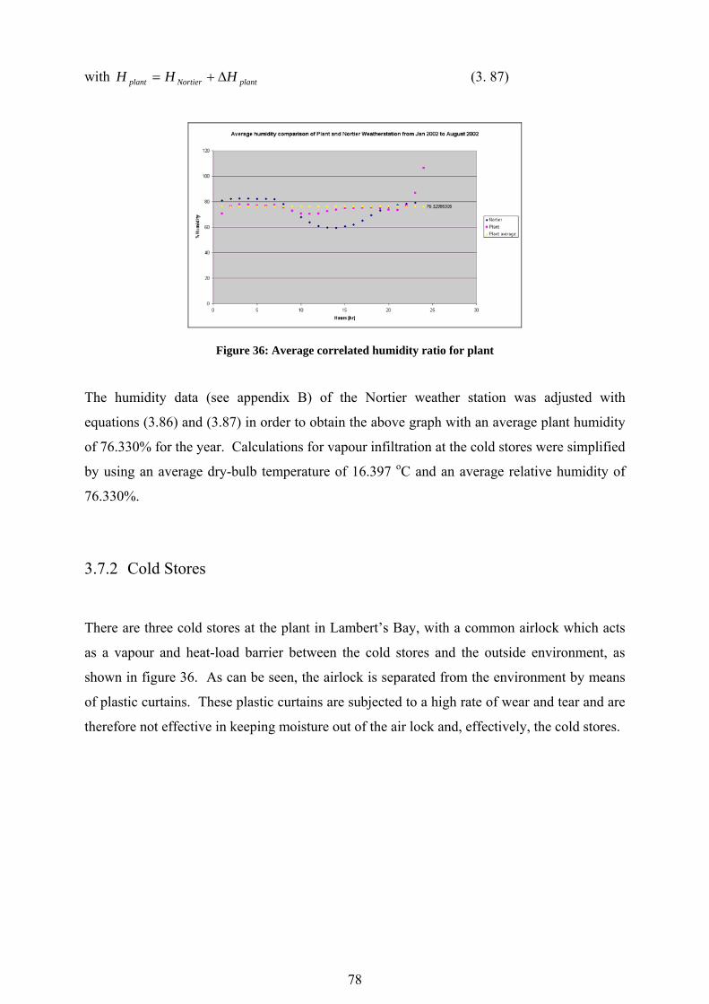
78

with plantNortierplant HHH Δ+= (3. 87)

Figure 36: Average correlated humidity ratio for plant

The humidity data (see appendix B) of the Nortier weather station was adjusted with

equations (3.86) and (3.87) in order to obtain the above graph with an average plant humidity

of 76.330% for the year. Calculations for vapour infiltration at the cold stores were simplified

by using an average dry-bulb temperature of 16.397 oC and an average relative humidity of

76.330%.

3.7.2 Cold Stores

There are three cold stores at the plant in Lambert’s Bay, with a common airlock which acts

as a vapour and heat-load barrier between the cold stores and the outside environment, as

shown in figure 36. As can be seen, the airlock is separated from the environment by means

of plastic curtains. These plastic curtains are subjected to a high rate of wear and tear and are

therefore not effective in keeping moisture out of the air lock and, effectively, the cold stores.

79

Cold store 3

Cold store 1

Cold store 2

Environment

Environment

Airlock

Figure 37: Cold stores and airlock

Losses at the cold stores can be ascribed to three factors:

1. Sensible heat load from the environment.

2. Vapour transfer due to infiltration and convection mass transfer from outside.

3. Sensible heat load from forklifts, forklift drivers and the product.

The first two activities will be discussed in this chapter.

Sensible Heat Load from Environment

Sensible heat enters the cold stores from the environment through radiation and natural or

forced convection. Insulation panels limit the amount of heat entering the cold store. The

insulation panels are constructed from chromadeck steel plates with polystyrene foam

inbetween the plates. The steel plates also act as a vapour barrier. The moisture in the air

wants to diffuse to the cold store due to a difference in vapour pressure and, when the outside

steel plates are damaged, vapour enters through the hole and condenses at the dew-point

temperature mark inside the polystyrene layer and freezes at 0 °C inside the insulating panels.

The ice that builds up inside the insulating panel, fills the air volumes in the polystyrene,

thereby decreasing the insulation effect of the panel and resulting into a higher sensible heat

load. By calculating the new overall heat transfer coefficient and comparing it with the

80

design value of the insulating panel, it is possible to estimate the extra amount of heat that

needs to be removed.

Radiation and convection heat transfer cause a sensible heat load for the cooling room.

Where the cold store’s panels are subject to sunrays, radiation will play a much bigger role

than on the inside where the only radiation is diffuse radiation to the surrounding air.

T pi

T dbo T wboV wind

T i

T po

q rado + qconvo

q radi + q convi

Figure 38: Insulating panel with indication of temperature gradient

By measuring the dry and wet-bulb temperatures of the outside environment, as well as the

dry-bulb temperature inside the cold store and the surface temperatures of the plates, it is

possible to calculate the approximate heat transfer rate, qtotal, through the insulating panel.

From this results, it is possible to calculate the overall heat transfer coefficient, Uoverall.

( )pipooveralltotal TTUq −⋅= (3. 88)

Tpo is the outside surface-plate temperature and Tpi the inside surface-plate temperature.

From a correlation in Mills (1995), the emissivity of the sky can be calculated:

⎟⎟⎠

⎞⎜⎜⎝

⎛⋅+=

atm

vsky P

P8.155.0ε (3. 89)

The thermo-physical properties of moist air were calculated from correlations in Kröger

(1998), with the specific humidity, ω, read from the psychometric chart. The Prandtl number

is calculated as follows:

81

avo

avopavo

kc μ⋅

=Pr (3. 90)

where cpavo is the specific heat of the moist air, μavo the dynamic viscosity of moisture and kavo

the thermal conductivity of moist air. On a windless day, natural convection will take place

and laminar and turbulent flow on a vertical plate equations will be used.

The Prandtl number function,

916

169

Pr492.01

−

⎥⎥

⎦

⎤

⎢⎢

⎣

⎡⎟⎠⎞

⎜⎝⎛+=Ψ (3. 91)

is needed to determine the Nusselt number for natural convection. In natural convection, flow

is initiated through density variation (buoyancy) caused by temperature difference, which is

brought into account with the volumetric expansion coefficient,

( ) ( )( )( ) ( )dbopopoavo

dboavopoavo

TTTTT

−⋅

−−=

ρρρ

β (3. 92)

The Grashof number at a position x from the bottom of the wall is:

( ) ( )( )( )2

3

dboavo

dbopox T

xgTTxGr

ν

β ⋅⋅−⋅= (3. 93)

where νavo(Tdbo) is the kinematic viscosity of moist air calculated at dry-bulb temperature.

With the Grashof number known at the full length of the plate, it is possible to calculate the

Rayleigh number:

( ) ( )dboLdboL TGrTRa Pr⋅= (3. 94)

With the Rayleigh number known, the laminar and turbulent Nusselt numbers can be

calculated respectively:

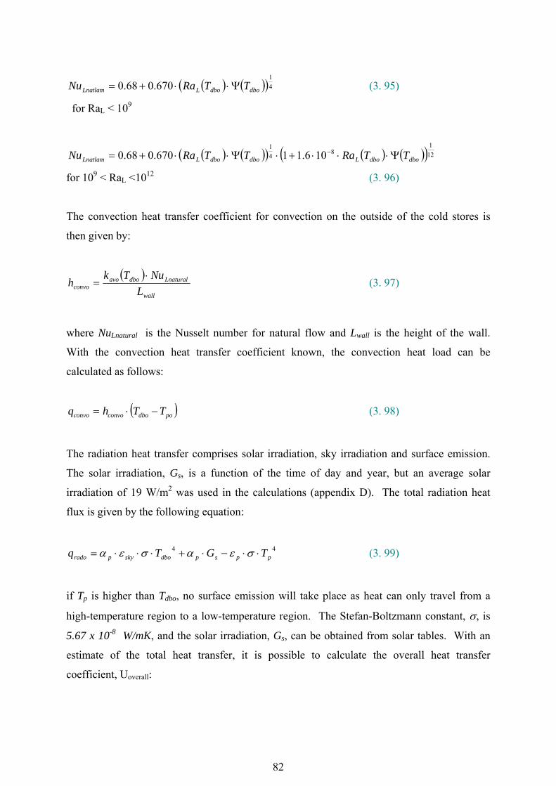
82

( ) ( )( )41

670.068.0 dbodboLLnatlam TTRaNu Ψ⋅⋅+= (3. 95)

for RaL < 109

( ) ( )( ) ( ) ( )( )121

841

106.11670.068.0 dbodboLdbodboLLnatlam TTRaTTRaNu Ψ⋅⋅⋅+⋅Ψ⋅⋅+= −

for 109 < RaL <1012 (3. 96)

The convection heat transfer coefficient for convection on the outside of the cold stores is

then given by:

( )wall

Lnaturaldboavoconvo L

NuTkh

⋅= (3. 97)

where NuLnatural is the Nusselt number for natural flow and Lwall is the height of the wall.

With the convection heat transfer coefficient known, the convection heat load can be


( )podboconvoconvo TThq −⋅= (3. 98)

The radiation heat transfer comprises solar irradiation, sky irradiation and surface emission.

The solar irradiation, Gs, is a function of the time of day and year, but an average solar

irradiation of 19 W/m2 was used in the calculations (appendix D). The total radiation heat

flux is given by the following equation:

44

ppspdboskyprado TGTq ⋅⋅−⋅+⋅⋅⋅= σεασεα (3. 99)

if Tp is higher than Tdbo, no surface emission will take place as heat can only travel from a

high-temperature region to a low-temperature region. The Stefan-Boltzmann constant, σ, is

5.67 x 10-8 W/mK, and the solar irradiation, Gs, can be obtained from solar tables. With an

estimate of the total heat transfer, it is possible to calculate the overall heat transfer

coefficient, Uoverall:

83

podbo

radoconvooverall TT

qqU

−+

= (3. 100)

This value can be compared to the design value of the insulation panels, which is obtainable

from the manufacturer or can be calculated if the physical composition is known. The design

overall heat transfer coefficient is calculated as follows:

1

2−

⎥⎥⎦

⎤

⎢⎢⎣

⎡ ⋅+=

s

s

p

pdesign k

tkt

U (3. 101)

where tp is the thickness of the polystyrene – 150 mm, ts the thickness of the steel plates, kp

the thermal conductivity of polystyrene foam as obtained from the manufacturer and ks the

thermal conductivity of steel. For the southern side of the cold stores, an extra layer of 50

mm insulation panels were added, and the design value was calculated as follows:

1

4−

⎥⎥⎦

⎤

⎢⎢⎣

⎡ ⋅+=

s

s

p

pextrahdesignsout k

tk

tU (3. 102)

where tpextra = 200 mm. The percentage decrease, which is an indication of the decrease in

sensible heat load, is calculated as follows:

100% ⋅=actual

design

UU

Decrease (3. 103)

From the measurements taken, a theoretical improvement of 951% is possible by replacing

the insulating panels that are filled with ice.

Vapour Infiltration

Due to the significantly lower temperature of the cold stores, the vapour pressure is much

lower in the cold stores than in the outside environment (ideal gas law). This difference in

pressure causes the vapour molecules to travel from a high-pressure region (in this case the

outside environment) to a low-pressure region (in this case the cold stores), resulting into frost

build-up on the evaporator coils in the cold stores.

84

The driving force behind mass transfer is the partial pressure difference between the outside

air and the cold stores. In order to estimate the annual energy costs of vapour infiltration,

mass transfer calculations were done by approaching the problem as diffusion of one gas

(water vapour) through a second, stagnant gas (dry air) with a lower concentration of water

vapour. Fick’s law for ideal gases with negligible pressure gradient states:

⎟⎟⎠

⎞⎜⎜⎝

⎛⋅⋅=

ρρ

ρ νB

B dydDJ (3. 104)

where JB is the diffusive mass flux, Dν the proportionality factor and ρ

ρ B the mass fraction.

Figure 39: Infiltration effect

Let us assume the mass will be transferred from the passage to the cold store, given by the

following equation:

⎟⎟⎠

⎞⎜⎜⎝

⎛⋅⋅+⎟⎟

⎠

⎞⎜⎜⎝

⎛⋅⋅−=

p

Bppp

c

BcccBnet dy

dDdydDJ

ρρ

ρρρ

ρ νν (3. 105)

simplifying the problem by letting the passage and cold store each diffuse separately into a

100% dry air area, subtracting the cold store’s mass flux from the passage to give net water

vapour mass flow into the cold store. The interface where mass transfer occurs is the door

opening where, after it is opened, the gradient tends to infinity. The mass fraction can be

written as a specific humidity fraction, which makes it easier to handle:

85

1+==

ωω

ρρ

t

BB

mm (3. 106)

Thus, the net mass flux can be rewritten as follows:

⎟⎟⎠

⎞⎜⎜⎝

⎛

+⋅⋅+⎟⎟

⎠

⎞⎜⎜⎝

⎛+

⋅⋅−=11 p

ppp

c

cccBnet dy

dDdydDJ

ωω

ρω

ωρ νν (3. 107)

The mass diffusivity is given by (Kröger, 1998):

⎟⎟⎠

⎞⎜⎜⎝

⎛

+⋅⎟⎟

⎠

⎞⎜⎜⎝

⎛⋅

=2451000

926.0 5.2

db

db

atm TT

PDν (3. 108)

with Patm in Pa and Tdb in K. Finally, the mass transfer rate can be calculated:

Bnetdoortransfer JAm ⋅= (3. 109)

The above calculations are for diffusion only and do not include convection mass transfer. As

the forklift enters the airlock through the plastic curtains, it generates air movement inside the

airlock and if the doors of the cold stores are open, convection mass transfer occurs, resulting

in a larger amount of water vapour inside the cooling room that needs to be removed by the

evaporators.

The energy cost of 1 kg of water vapour was calculated. The energy needed to freeze water

from vapour to ice is the difference between the enthalpy value of the water vapour at the

outside air’s dry-bulb and wet-bulb temperature and the enthalpy value of ice at the

evaporator temperature.

The enthalpy of vapour and ice is given by the following equations respectively:

( )KTKkg

kJkgkJh dbv 15.273805.12501 −⋅

⋅+= (3. 110)

dewpiceice Tch ⋅= (3. 111)

86

where cpice is 1.860 kJ/kgK and Tdew is the temperature of the evaporator coil, assumed to

approach dew point. The energy needed to freeze a certain mass of water, mwater, is:

( ) operatingicevwaterfreeze thhmE ⋅−⋅= (3. 112)

where toperating is the period that the cold stores are in operation during the year and mwater is

the average mass of water condensed through the year. The number of kWh units can then be

obtained by dividing Efreeze by 1 kWh, whereas the electricity costs are obtained by using an

average cost per unit for the year and assuming the cooling rooms are operative 24 hours per

day. Payback calculations were done (see appendix G) to motivate the capital expenditure for

air curtains, which can be assumed to work with an effectiveness of 70% to 90%.

3.7.3 Flow Freezer

The flow freezer (see figure 40) is on the production line and freezes the French fries as they

enter from the precooler, which uses outside air to precool the French fries. The fries enter at

approximately 20 oC and exit at approximately –16 oC.

3 1 5 0 .0 0 s q m m

8 0 9 9 .9 8 s q m m

Figure 40: Schematic representation of flow freezer

Air inside the flow freezer is circulated across a plate heat exchanger by means of an axial

fan. Losses that occur at the flow freezer are almost similar to those at the cold stores, except

87

that in the flow freezer’s case, the largest energy losses are due to vapour condensation on the

heat exchanger, resulting in inefficient heat transfer from the heat exchanger to the circulating

air. This effect causes the fan to work harder, resulting in shorter motor life and higher fan-

power requirements.

To keep moisture out of the flow freezer one must keep the inside pressure slightly higher

than the outside pressure and add pressure drop obstructions between the outside air and the

circulating air. Moisture infiltration at the flow freezer is a significant energy loss factor.

3.7.4 Blast Freezer

The blast freezer is a batch freezer. It removes sensible heat from the packaged product as it

is removed from the production line. The temperature of the product needs to be lowered

from –6 oC to –25 oC before it is stored in the cold stores, especially if it is to be transported

in the next two days. The blast freezer works on the same principle as the flow freezer,

except that the packaged product is static inside an enclosed volume. To minimise energy

losses, the insulation must be kept in good shape and the door must seal properly. Valuable

refrigeration capacity is destroyed when hot, humid air infiltrates the freezer and cold, dry air

leaves into the factory environment, which is also undesirable. This effect can be minimised

through plastic curtains at the openings of the blast freezer.

3.7.5 Refrigeration Pipes

Heat loss calculations of the refrigeration insulation were conducted by measuring the surface

temperature on various points on the insulation and assuming natural convection in the still air

of the plant. The calculations that were done to determine the energy loss are shown below.

Assuming natural convection for the refrigeration pipes inside the plant, measurements of the

outside temperature on the refrigeration pipes were estimated by means of a Raytek infrared

thermometer and the physical dimensions of the insulation were taken. The wet and dry-bulb

temperatures, Tdbplant and Tnbplant, for the inside of the plant were measured with a wet and dry-

88

bulb sling thermometer. The refrigeration pipes were divided into segments to simplify heat

gain calculations.

For natural convection over a horizontal cylinder, the Grashof, Nusselt and Rayleigh numbers

were calculated with:

dbplantT1

=β (3. 113)

KmWk⋅

= 026.0 (3. 114)

69.0Pr = (3. 115)

sm2

6107.14 −⋅=ν (3. 116)

2807.9smg = (3. 117)

where β is the volumetric coefficient of expansion, k the conductivity, Pr the Prandtl number

and ν the kinematic viscosity coefficient for air. The Grashof, Rayleigh and Nusselt numbers

are given by the following equations:

( )2

3

νβ ii

DidgT

Gr⋅⋅Δ⋅

= (3. 118)

Pr⋅= DiDi GrRa (3. 119)

( )94

169

25.0

Pr559.01

518.036.0

⎥⎥

⎦

⎤

⎢⎢

⎣

⎡⎟⎠⎞

⎜⎝⎛+

⋅+= Di

DiRa

Nu (3. 120)

With the Nusselt number known, the heat transfer coefficient can be found:

89

i

Dici d

Nukh ⋅= (3. 121)

and the heat gain is calculated as follows:

iicii TAhQ Δ⋅⋅= (3. 122)

The area, Ai, was estimated as a percentage of the full area of the segment at a certain

temperature. The total heat gain for all the refrigeration pipes were added up to determine the

number of kWh units lost. Assuming fairly uniform operation over 24 hours, an average price

per kWh unit was estimated in order to calculate the savings possible per time period, Sp. For

Ip, the interest rate for the duration of the period and n, the number of periods, the payback

period can be calculated. Calculations done in appendix A illustrate that, with the current

savings and a payback period of 10 years, R3 682 can be spent, which is much less than

necessary.

3.8 Product Lifecycle Analysis

Improving the efficiency of the production line not only increases productivity, but also leads

to energy and salary savings (Energy Research Institute, 2000). In the figure below a flow

diagram of the production line is shown, indicating the various processes in the production

line. Specifications for the finished product allows 2% of the finished product to be defective.

It is estimated that 60% of incoming defects are removed at inspection belt 1 and 40% is

removed at inspection belt 2. Currently, 10 workers (six at inspection belt 1 and four at

inspection belt 2) are needed to remove the defects manually. From estimations in 2001, the

incoming defects before removal for 60% of the time are 15% of the incoming product and

the inspection belts can reach specification (2% defects allowed). For 15% of the time the

incoming defects are less than 10% and the inspection belts meet specification, and for the

next 25% of the time the incoming defects are 20% and 4% defects are in the final product,

unable to reach specification.

90

Figure 41: Production process line

The total defects removed from the production line in a year amount to 12.55%, of which

60% (7.53% defects) is removed at inspection belt 1 and 40% removed at inspection belt 2.

By maximising the percentage of defects removed at inspection belt 1, less defects will move

through the production line absorbing unnecessary energy. This will lead to less product flow

through blancher 1, blancher 2, the predryers, dryers 1 to 6, the fryer, the de-fatter, the

precooler, the flow freezer and the shaker. In turn, this will lead to less steam, refrigeration

energy and electricity wasted on defective products that are thrown away. It also shortens

inspection line 2, because fewer workers are needed to pick out defects which in turn leads to

less exposure of frozen product to the warmer environment. It will also save the salaries of

six workers on inspection belt 1 and three workers on inspection belt 2. This could be

achieved by implementing an optical sorter.

Optical Sorter Modification in Production Line

An optical sorter will practically remove all the defects at inspection belt 1 (see figure below),

whereas only 0.1% of the defects will need to be removed at inspection belt 2 or it could be

left to fit into specifications.

91

Figure 42: Production line with optical sorter modification

The optical sorter will lead to the removal of 4.92% of the defects from the production line –

defects which were previously processed. The coal savings amount to R110 801.30 per year,

the electricity savings amount to R5 151.46 and savings from less labour amount to R587 500

per annum (see appendix I). By estimating maintenance at 10% of the optical sorter’s value

for the first five years and subtracting this value from the total savings, the payback period of

the equipment can be determined:

( )1003.3

17.01ln

17.076.573452

103.11

1ln 6

=+

⎟⎟⎟⎟

⎠

⎞

⎜⎜⎜⎜

⎝

⎛

⋅⋅

−=

n

n (3. 123)

With the inclusion of maintenance estimates, the optical sorter will be paid off in three years’

time.

92

3.9 Waste Utilisation

Potato-related wastage caused by processes in the production line can be utilised in many

different ways. One of them is the production of ethanol from potato waste. The figure

below shows where the waste of the de-skinner exits the plant. Currently, outside contractors

are employed to remove the potato waste.

Figure 43: Potato waste from steam peeler at plant

However, these waste products can be used for alcohol production, where the alcohol can be

used to generate steam or dry a part of the potato waste and sell it as animal food. Since the

oil crisis of 1973 and 1979, the significant rise in oil prices have led to research of alternative

energy sources, of which the potential alcohol yield of potatoes were determined. The

potential alcohol yield of 1 ton potatoes is 600 litre. The daily potato wastage at the plant is

approximately 10 ton. Let us assume the alcohol conversion process can be done at 80%

efficiency. The alcohol yield is 600 l/ton potatoes. The volume of alcohol that can be

produced daily is as follows:

daylVmYieldV

alc

wastealcutilconalc

/4560=⋅⋅⋅= &ηη

(3. 124)

Assuming that the alcohol conversion process is an optimised one, which (according to

Misselhorn, K. Oktoberagung der Wersuchs - und Lehranstalt Fur Brauerei) needs an energy

input of 8 MJ per litre of dry ethanol, where the higher heating value of ethanol is 30.61

93

MJ/kg of ethanol, there is a positive excess amount of energy available for other use. Let us

assume that after distillation, the ethanol is at a temperature of 20 oC, with a density of 789

kg/m3, then the energy potential of the ethanol amounts to:

MWEnergyL

mmkg

LMJ

kgMJ

Lm

mkg

sLEnergy

eHHVVEnergy

EEEnergy

produced

produced

alc

inalcalcalcproduced

inoutproduced

011809.1

001.0789861.30001.078905278.03

3

3

3

=

⎟⎟⎠

⎞⎜⎜⎝

⎛⋅⋅−⋅⋅⋅=

⎟⎟⎠

⎞⎜⎜⎝

⎛−⋅⋅=

−=

ρρ

(3. 125)

The amount of coal that can be saved annually through the production of ethanol amounts to

R380 000.

94

4 CONCLUSION

Analyses of the steam dryers in section 3.6.1 identified the source of ineffective operation and

it was found that improved housekeeping could lead to an increased effectiveness to

accommodate a higher production rate.

The implementation of a flash-steam heat recovery system at the boiler will lead to a monthly

energy saving of almost R14 000,00 with a payback period of 3.3 years at a capital cost of

R44 206,00.

The recovery of waste steam at the steam peeler with the implementation of a finned-tube heat

exchanger in the deceleration duct will lead to a monthly energy cost saving of R8 675 with a

payback period of 14.19 months at a capital cost of R110 836,00.

Measurements and heat load calculations for the insulating panels of the cold stores indicated

that damaged insulation panels have a dramatically lower insulation effect due to ice

formation inside and, thus, a higher heat conduction coefficient. Vapour infiltration also leads

to a higher heat load and maintenance cost (forklift accidents on slippery floor). The

implementation of air curtains will decrease vapour infiltration by 80% and have a payback

period of 1.791 years, based only on energy savings at a capital cost of R9 900,00.

Analyses of production line modifications (see section 3.8) showed that, through the

improvement of the inspection process earlier in the line by implementing an optical sorter,

labour and energy savings will amount to R573 452 per annum and have a simple payback

period of 3.1 years.

A preliminary study of waste utilisation showed that an in-depth analysis of ethanol

production from potato waste is needed to prove the feasibility.

Future research can be conducted on the acquisition of an optical sorter and on improvements

on the production line to minimise energy losses due to radiation.

95

REFERENCES

ASHRAE, 1997, Handbook 1997 Fundamentals, American Society of Heating, Refrigerating

and Air-conditioning Engineers.

ASHRAE, 1993, Handbook 1993 Fundamentals, American Society of Heating, Refrigerating


ASHRAE, 1984, Handbook 1984 Systems, American Society of Heating, Refrigerating and

Air-conditioning Engineers.

Bagajewicz, M.J., 2001, Process Plant Instrumentation: Design and Upgrade, Technomic

Publishing Company.

Benelmir, R. & Feidt, M., 1998, Energy cogeneration systems and energy management

strategy, Energy Conversion Management, Volume 39, 1791 – 1802.

Blanchard, B.S. & Fabrycky, W.J., 1998, Systems Engineering and Analysis (3rd edition),

New Jersey: Prentice Hall.

Çengel, Y.A. & Boles, M.A., 1994, Thermodynamics: an Engineering Approach, McGraw-

Hill.

Dutch National Team, 2000, Heat recovery from discharge steam in the food industry,

CADETT Energy Efficiency, Newsletter No. 1, 10 – 11.

Energy Research Institute, 2000, How to save energy and money: The 3E Strategy, University

of Cape Town, South Africa.

Fabrycky, W.J., Thuesen, G.J. & Verma, D., 1998, Economic Decision Analysis, Prentice

Hall.

96

Garrote, R.L., Silva, E.R. & Bertone, R.A., 2000, Effect of thermal treatment on steam peeled

potatoes, Journal of Food Engineering (45), 67 – 76, Elsevier.

Greenberg, M.D., 1998, Advanced Engineering Mathematics (2nd edition), Prentice Hall.

Kreith, F. & West, R.E., 1997, CRC Handbook of Energy Efficiency, CRC Press.

Kröger, D.G., 1998, Air-cooled Heat Exchangers and Cooling Towers

Maréchal, F. & Kalitventzeff, B., 1998, Energy integration of industrial sites: tools,

methodology and application, Applied Thermal Engineering (18), 921 – 933, Pergamon.

Marshall, T., 2002, Keeping costs down with a frost-free cold store environment, The South

African Mechanical Engineer, Volume 52, 23 – 24.

Mills, A.F., 1995, Heat and Mass Transfer, Irwin.

Rockwell, T.C. & Quake, T.D., 2001, Improve refrigeration system efficiency, Process

Cooling & Equipment.

Schmidt, E., 1969, Properties of water and steam in SI-units, New York: Springer.

Singh, A.K., Singh, H., Singh, S.P. & Sawhney, R.L., 2001, Numerical calculation of

psychrometric properties on a calculator, Building and Environment, Volume 37, 415 – 419,

Elsevier.

Stewart, A., 2001, Cold is gold, Refrigeration and Air-conditioning, 35 – 41, South Africa,

October.

Turpin, J., 2000, So, how do you keep frost, ice out of warehouses?, Air Conditioning,

Heating and Refrigeration News.

Uticon-Dynatherm Industrie bv, 1994, Energy Calculations: Lambert’s Bay Canning

Company.

97

Zhuwakinyu, M., 2001, Ghana leads in energy efficiency, Martin Creamer’s Engineering

News, August 24 – 30.

98

BIBLIOGRAPHY

ASHRAE, 1982, Handbook 1982 Applications, American Society of Heating, Refrigerating


ASHRAE, 1994, Handbook Refrigeration Systems and Applications, SI Edition.

A Spirax Sarco guide, 1982, Steam quality and steam consumption, Printed in England.

A Spirax Sarco guide, 1982, Steam and steam trapping, Printed in England.

Australian National Team, 1999, Efficient cold store facility for Albany Port Authority,

CADETT Energy Efficiency, 22 – 23, Special Issue on Australia.

Beek, W.J., 1999, Transport phenomena, New York.

Bejan, A., 1996, Entropy Generation Minimization, CRC Press.

Bejan, A., 1988, Advanced Engineering Thermodynamics, John Wiley & Sons.

Bolton, W., 1991, Newnes instrumentation and measurement pocket book, Oxford.

Cecil, J.E, 1992, Small, medium and large-scale starch processing, Food and Agriculture

Organization of the United Nations.

Cussler, E.L., 1984, Diffusion: mass transfer in fluid systems, Cambridge University Press.

D'Accadia, M.D. & De Rossi, F., 1998, Thermo-economic optimisation of a refrigeration

plant, International Journal of Refrigeration, Volume 21, 42 – 54.

Fahien, R.W., 1983, Fundamentals of transport phenomena, New York: McGraw-Hill.

Finney, R.L. & Thomas, G.B., 1994, Calculus (2nd edition), Addison-Wesley.

99

Kays, W.M. & Crawford, M.E., 1993, Convective Heat and Mass Transfer, McGraw-Hill.

Lisinska, G., 1989, Potato science and technology, London: Elsevier Applied Science.

Masters, G.M., 1998, Introduction to Environmental Engineering and Science, Prentice Hall.

Nikolaides, C. & Probert, D., 1998, Exergy-method analysis of a two-stage vapour-

compression refrigeration-plants performance, Applied Energy (60), 241 - 256, Elsevier.

Norris, P.E., 1954, About yeast, London: Thorsons.

Rosaler, R.C., 1998, HVAC maintenance and operations handbook, New York: McGraw-Hill.

Stoecker, W.F. & Jones, J.W., 1982, Refrigeration & Air Conditioning, McGraw-Hill.

Talburt, W.F. & Smith, O., 1987, Potato processing, New York: Van Nostrand Reinhold.

Spencer, J.F.T. & Spencer, D.M., 1990, Yeast technology, Berlin: Springer.

Spencer, J.F.T. & Spencer, D.M., 1997, Yeasts in natural and artificial habitats, Berlin:

Springer.

Van Beynum, G.M.A. & Roels, J.A., 1985, Starch conversion technology, New York:

Dekker.

100

A APPENDIX: ELECTRICITY, COAL AND PRODUCTION RECORDS

101

A.1 Electricity Readings

Date

23/02/2002

Equipment Current [Amp] Watt

Transformer 1 1030 391400

Transformer 2 750 285000

1780 676400

FES Compressor 280 106400

M&M Compressor 2 320 121600



Boiler electricity 45 17100

Refrigeration electric motors 115 43700

Production line 533 202540

Total electricity 676400

Total refrigeration 456760

Coal energy usage rate [kg/day] Watt

Calorific value of coal [J/kg] 27320000

Coal usage: 13 bags at 850kg each 11050 3494050.926

Table A. 1: Electricity readings and coal usage

102

A.2 Electricity and Coal Consumption

Electricity usage and costs

Off-peak 0.0859 Energy unit

Peak 0.3923 J

Standard 0.148 3600000

Usage

Off-peak Peak Standard Electricity cost

Coal price

R/kg Calorific value

December 346863 126359 315192 126014.5834 447.5 J/kg

January 408974 142368 380440 147286.953 28500000

February 361300 143830 354365 139906.199

March 352922 134165 337495 132898.1893

April 442585 158377 418115 162030.3686

May 479331 172953 422610 171570.2748

Last 4 months 1636138 609325 1532585 606405.0317

Average 151601.2579

Unit price 0.160507498

Energy comparison

Coal usage Coal cost Elec. Elec. cost/MJ Coal Coal cost/MJ Unit elec. Unit coal

MJ MJ

January 1420799.5 635807.7763 3354415.2 0.043908385 40492785.75 0.015701754 0.86685943 0.91002922

February 1085001.5 485538.1713 3094182 0.045215892 30922542.75 0.015701754 0.799609078 0.694948913

March 1133679 507321.3525 2968495.2 0.044769548 32309851.5 0.015701754 0.767128666 0.726127097

April 1469148 657443.73 3668677.2 0.044165883 41870718 0.015701754 0.948072089 0.940996677

May 1561268 698667.43 3869618.4 0.044337776 44496138 0.015701754 1 1

2348970.684 13600972.8 0.044585416 149599250.3 0.015701754

Average 587242.6709 3400243.2 0.044585416 37399812.56 0.015701754

Table A. 2: Electricity and coal consumption data for January 2002 till May 2002

103

A.3 Electricity, Coal and Production Comparison

Electricity, coal and production comparison

Month

Electricity

usage Coal usage

Production

rate raw Yield

MJ MJ kg/month

January 3354415.2 40492785.75 2543684 55.9%

February 3094182 30922542.75 1980374 58.1%

March 2968495.2 32309851.5 2042707 54.5%

April 3668677.2 41870718 2609655 56.0%

May 3869618.4 44496138 2719978 57.4%

Average 3391077.6 38018407.2 2379279.6

Electricity, coal and production comparison on a unit basis

Month Electricity Coal Production

January 0.989188569 1.065083698 1.069098394

February 0.912448008 0.813357135 0.832341857

March 0.875384037 0.849847584 0.858540123

April 1.081861766 1.101327517 1.096825695

May 1.14111762 1.170384066 1.143193931

Electricity, coal and production comparison on a unit basis

Month Dry-bulb [oC] Humidity Unit Dry-bulb Unit Humidity

January 18.5375 75.625 1.015753425 1.051564311

February 21.0125 64.29166667 1.151369863 0.893974508

March 19.70833333 69.75 1.079908676 0.969872538

April 17.275 73.25 0.946575342 1.018539977

May 14.71666667 76.66666667 0.806392694 1.066048667

Average 18.25 71.91666667

Table A. 3: Electricity, coal and production for January 2002 till May 2002

104

A.4 Walkthrough Audit Checklist

Walkthrough audit checklist

Auditor: ________________ Date: ________________

Fuel, gas or oil

leaks

Steam leaks

Condensate leaks

Water leaks

Damaged or leaking

insulation

Excess utility usage

Equipmant running and not

needed

Burners out of

adjustment

Leaks of or excess

of HVAC

Location

105

B APPENDIX: NORTIER TEMPERATURE AND HUMIDITY DATA

106

B.1 Nortier Temperature Data

Hours of the day – Nortier temperature data January 2002 – August 2002

Day 1 2 3 4 5 6 7 8 9 10 11 12 13 14 15 16 17 18 19 20 21 22 23 24

1 14.7 14.7 14.7 15.1 13.7 13.5 16 18.8 19.8 21.4 21.8 21.5 22 21.8 21.6 21.7 20.5 19.5 19.1 17.6 17.4 16.7 16.3 15.7

2 14.7 14.6 13 13.1 12.6 12 16.1 18.4 19.6 21 23.8 23.9 23.2 24.1 24.3 25.3 24 25.2 22.7 21.2 20.3 19.6 19.5 16.7

3 14.9 13.8 13.7 13.8 14.1 13.6 14.9 16.7 17.8 20 19.1 23.4 22.4 23.6 23.9 26.3 22.1 21.9 21.4 19.2 17.6 17 16.5 14.1

4 13.1 12.5 13.2 14.1 13.8 11.7 14.6 17.7 21.8 20.6 21.5 21.6 22.3 23.2 23.9 25.2 21.6 20.5 18.3 17.9 17.2 16.9 16.1 15.4

5 15.3 13.8 14.9 15.7 15.7 15.7 16.2 16.6 17.4 19 21 22.1 22.8 23 23.1 22.1 22.5 21.5 20.2 18.3 17.6 17.5 16.5 17.6

6 17.8 17.8 16.4 16.8 16.5 15.4 14.5 14.9 16.6 16.8 17.2 18.7 18.6 19.9 20.1 20.2 20.1 19.6 18.1 16.5 15.4 15 12.9 11.8

7 11.5 11.7 13.4 13.4 13.1 13.2 12.8 14.6 16.3 17.4 18.2 18.5 18.2 19.6 19.5 19.3 19.3 18.6 17.1 15.8 15.1 14.3 13.7 13

8 13 12.4 11.5 10.9 11.1 11.4 14.1 17.3 19.4 20.7 20.4 21.7 21.1 22.3 22.3 22.1 20.7 20.5 20.7 18.8 17.5 16.5 15.9 14.9

9 14 13.7 13.1 11.2 10.8 10 13.5 16.4 19.6 19.8 20.3 20 20.7 21.8 21.5 21.6 20.9 19.9 17.9 16.5 15.7 15.1 14.8 14.6

10 15.2 15.5 14.6 15.3 15.6 15.4 15.9 17.5 19.4 21.3 22.2 21.7 21.7 21.8 21.6 21.9 22 21.2 19.8 18.1 17.3 16.2 14.9 13.8

11 15.3 15.1 14.3 16.1 16.9 17.1 17.9 19.1 19.9 17.5 17.4 17.1 17.9 20.2 19.4 19.6 18.1 17.2 17.9 16.3 15.9 15.3 15.6 15

12 15 14.6 14 14.1 13.7 12.6 13.8 16.1 17.8 19.4 20.4 20.6 20.7 21.4 20.9 21.1 20.8 19.5 18.5 17 15.6 15 14.5 13.9

13 13.9 13 12.8 12.9 11.8 11.5 14.3 18.2 21.3 20.5 21.8 22 23.2 22.5 22.5 22.2 21.8 20.5 19.7 18.1 17.1 16.4 15.5 15

14 14.1 13.5 11.9 11 10.6 10.4 12 16.6 19.6 20.5 21.3 21.4 21.2 21.8 21.6 21.4 21 20.2 18.9 17.5 17.2 16.7 16.2 15.8

15 15.1 14.5 13.2 13 12.2 14.2 14.2 15 18.1 19.8 20.4 20.6 20.9 22.3 22.9 22 21.3 20.8 19.3 17.9 17.2 16.8 16.5 15.7

16 15.3 15.6 13.1 13 13.8 15.2 16.5 17 16.7 18.9 20.7 21.9 22.6 22.5 22.1 21.9 21.1 20.6 19.5 18 17.4 18 16.3 16

17 15.5 16.1 15.9 15.1 14.4 14.4 15.1 16.4 17.7 18.9 18.3 16.2 17.8 17.6 16.8 16.5 17.8 18.1 17.3 16.8 15.6 15.1 14.8 15.3

18 15.6 15.3 14.7 14.5 13 12.9 14.5 17.6 19 19.8 20.3 20.3 20.8 20.9 21 20.7 20.6 19.8 19.3 18.3 18.1 18 17.4 16.9

19 16.4 15.6 15.4 14.6 14.2 13.1 15.4 17.5 19.8 21.7 22.3 23 22.3 23.7 23.1 23.3 22.1 21.1 19.2 18.4 18 17.5 16.6 16.1

20 16.2 16.2 15.1 14.4 12.5 12.1 15.1 17.5 19.3 20.3 20.7 21.8 21.9 22.8 22.5 22.2 21.5 20.9 19.8 18.3 18.1 18.1 18.1 17.7

21 16.6 16.1 15.7 15.4 15.5 15.5 16.7 19.7 21.7 21.7 22.8 23.4 23.4 22.8 23.3 22.2 21.7 21.5 20 19 19.1 18.5 18.2 18

22 17.5 16.7 16.5 16.2 16.2 16.8 17.4 18.3 20.9 21.8 23.2 23.9 24.5 23.9 24.4 22.4 21.8 21.2 19.8 19.3 19 19.5 19.6 19.2

23 18.2 17.7 17.9 17 16.5 16.2 17.9 21.5 22 21.6 23.4 24 23.9 23.5 23.3 23.1 22.2 22.7 21.4 19.4 18.7 17.2 16.6 15.8

24 15.1 14.8 14.8 14.1 12.8 13.9 14.9 17.7 22.2 20.9 21.5 22.5 23.5 24.5 25.2 26.1 25.1 23.9 22.9 21.6 20.7 18.9 18.2 17.9

25 17.5 17.2 16.9 16.1 15.5 15.9 17.2 19.3 19.8 17.4 18.8 20.2 20.7 20.7 21.9 21.4 22.8 21.6 18.7 17.6 17.5 17.5 16.8 16.8

26 17.2 17.5 17 16.5 16.5 16.5 16.4 17.3 19.1 21.2 22.3 22.7 23 22.5 22.4 22.5 21.9 21.4 20.2 19.3 18.9 18.6 17.8 17.4

27 17.5 18.3 18.6 18.8 18.7 18.5 18.6 20 21 22.3 22.2 22.2 21.9 21.6 21.1 19.6 19.6 19.7 19.7 19.3 19.3 18.1 17.5 17.2

28 17.3 17.6 18.4 16.9 15.7 15.6 17.5 20.8 21.6 23.9 23.4 23.8 23.2 22.6 22.3 22.9 21.6 21.6 20.5 19.3 18.8 18.6 17.6 15.8

29 17.6 17.9 18.1 17.6 15.7 16.6 18.1 19.5 21.5 22.1 22.5 22.8 23 23.2 23.9 24.1 23 22.4 21.1 20.3 19.5 19 18.1 18.8

30 18.5 18.8 19 18.9 19 19 19.1 19.6 21.9 21.7 23.8 24.6 24 24.5 24.5 25.1 23.8 23.3 22.4 21.4 19.8 19 18.5 17.6

31 16.8 16 15.3 14.5 14.7 15 16.9 20.9 25.4 24.7 24.9 25.9 26.1 27.3 27.9 25.6 26.2 25.4 25.6 23.2 22.8 23.1 22.1 20.8

1 23.1 22.9 22.2 23.5 22.8 23.9 26.7 28.7 29.4 31.4 33.9 34.9 31.7 32.7 33.7 30.9 29.3 30.4 28.4 26.1 24.5 24.8 23.9 23.2

2 22.9 21.9 21.4 21.1 20.7 19.9 21.5 23.4 26.2 26 26.8 26.5 26.6 27.7 26.5 24.9 25.2 25.3 24.5 20.1 18.9 18.2 17.2 16.1

3 15.8 15.2 15.9 16.3 16.5 16.6 16.5 17.4 19.8 21 21.1 22.8 22.8 22.2 23.9 23.5 24.3 22.5 21.5 19.7 18.7 18.2 17.7 16.9

4 16.6 16.2 15.9 15.3 14.3 12.9 15.1 16.6 18 20 21.8 22.1 23 23.3 23 22 22.6 22.1 20.7 18.8 18.5 17.7 17.9 17.5

5 17 17 16 14.9 15.1 14.9 15.4 18.5 20 20 22.3 21.8 22.5 22.5 21.5 22.1 20.8 19.5 20 16.5 16.4 16.9 16.8 17.6

6 15.7 15.3 15.3 15.6 15.8 15.4 16.1 17.4 18.1 15.2 15.1 17.6 21.8 20.1 20.6 19.5 18.5 17.6 17 15.6 14.7 14.8 15.2 15.3

7 13.9 13 13.1 11.2 10 10.1 11.3 17.1 20.5 24.4 22.8 22.9 23.3 23 21.9 23.2 22.4 20.7 20.2 18.3 18 17.2 17.9 17.6

8 18.6 18.2 19 19 18.6 18.2 20.1 25.8 27.8 25.8 27.7 28.5 29.5 27.5 27.4 29 28.3 27 25.8 22 21.9 20.9 20.5 20

9 18.9 21.4 21.4 20 15.7 13.9 17.7 23.9 27.6 29.8 28.8 30.1 28.7 25.4 22.5 22.7 22.1 19.5 16.2 15.5 15.3 16.2 16.1 15.9

10 16 16.4 16.5 16.4 16.3 16.4 16.5 17.1 17.5 18 19.5 20.8 21.9 22.4 21.8 21.4 19.9 19.2 18.8 18 16.9 16.9 16.9 16.6

11 16.1 15.9 15.3 15.5 15.7 16.2 16.1 16.7 16.5 16.9 19.4 21.1 20.8 20.6 22.4 21.7 21.5 20.2 19.5 18.3 16.9 16.6 15.2 14.4

12 14.1 13.3 12.9 12 11.7 11.5 12 14.9 17.1 17.6 19.8 20.2 20.6 20.6 20.6 19.8 18.8 18 16.1 16.2 15.5 15 14.6 13.8

13 13.5 12.4 12.1 11.9 11.5 11.3 10.7 14.2 16.6 18.3 19.7 19.7 18.7 20.1 20.3 20.6 20.1 19.1 17.3 16.2 16.1 15.4 15.1 13.4

14 13.4 12.4 12.2 13.1 11.3 10.8 12.2 15.3 17.8 19.4 20.7 21 21.7 21.1 21.6 21.7 21.2 20 18.8 17 16.5 15.7 15.3 13.7

15 13.4 14.2 14.9 15.3 16.3 16.8 17.1 17.8 19 18.8 17.1 17.8 19.3 21.2 20.8 21.2 20.8 19.5 18.1 16.3 15.7 15.4 14.9 14.4

16 13.7 12.6 12.2 11.8 10.9 10.4 11.4 16.5 19.8 20.1 20.2 21.3 22.9 22.8 22.7 22.5 23 22.1 20.4 18.5 18 16.6 15.6 15.1

17 15.3 14.1 15.3 15 14.4 14.8 17 23.5 25.7 28.9 24.6 27.5 27.2 27.6 25.5 27.7 27.7 28.3 26.2 24 22.2 21.5 23.7 22.7

18 21.9 21.5 20 18.4 21.9 19.4 22.4 26.5 30.6 33.3 35.3 36.9 38.2 30 28.9 33 32.8 27.5 20.7 17.5 16.9 17.1 16.9 15.8

19 16.4 15.4 15.2 16.1 18.4 21.2 22.7 25.4 30.8 28.8 25.1 24 26.2 26.6 25 24.7 25.1 25.9 26.6 24.5 20.3 19.2 18.9 19.1

20 20.7 18.2 19.6 19.2 18.5 16.3 18.9 22.2 21.6 27.8 22 24 33 33.8 26.8 29.4 29.3 28.8 28.2 25.1 24.4 24.8 25 24.3

21 21.9 20.3 18.9 19.2 18.4 18.2 18.4 20.2 20.2 21.9 26.1 27.7 28.5 28.4 27.6 28.8 27.8 28 23.8 22.7 23.4 21.1 19.1 18.4

22 17.9 17.5 17.7 17.3 17.4 17.5 16.8 16.6 16.4 17.6 19.1 20.7 22.7 23.2 22.6 21.6 20.4 18.6 18.4 18.3 18.4 18.6 18.7 18.6

23 18.6 18.2 17 16.2 15.9 16 15.8 17.5 20.9 21.3 20.5 21.6 20.4 24.3 22 21.6 19.9 18.7 18.5 20.5 21.1 20.9 23.6 24.1

24 20.9 21.9 21.2 19.8 18.7 18.3 18.1 23.9 25.5 29.5 30.7 29.3 28.7 30.2 29.1 29.9 28.9 27 25.9 25.9 23.3 22.3 22.5 21.8

107


Day 1 2 3 4 5 6 7 8 9 10 11 12 13 14 15 16 17 18 19 20 21 22 23 24

25 20.9 19.9 19.4 18.9 19.8 21.2 21 23.2 26.9 29.9 28.2 30.7 30.4 29.7 33 31.8 29.9 29.2 27.8 26.5 26.3 25.5 24.8 25.4

26 23.5 22.2 22.4 22.6 23.9 26.5 25.8 29.7 33.7 35.3 36.4 38.3 40.3 40.3 33.7 35.3 29.1 29.7 28.6 28.6 27.8 27.8 25.1 23.4

27 20.9 20.4 20.5 21.3 21.2 21.3 21.4 22.9 23.8 28.7 25.2 28.2 24.2 27.6 22.5 23.1 25.5 26.2 26.6 22 22.2 22.5 22.3 22.3

28 23.3 20.7 20.3 20.4 21.5 21.8 20 21.9 22 18.9 20.2 20.9 24.4 29.2 26.2 25.6 24.6 25.2 21.2 20.5 20.1 19.4 18.8 18.7

1 18.5 18.1 18.2 17.6 18.3 18.7 18.5 20.3 21.3 23 24.3 24.7 24.4 24.4 24.5 23.9 24 22.6 21.2 20 19.6 19.4 19.1 18.9

2 18.6 18.4 17.9 18 17.4 16.5 16.3 17.1 17.4 18.1 20.9 22.1 23.2 23.2 23.1 23.1 22.8 21.9 20.4 19.4 19.6 19.3 19 18.9

3 16.3 15.8 16.1 16.1 16.6 16.1 15.9 18.1 21.8 21.8 23.4 24.7 24.9 24.7 24.5 24.4 24.5 23.8 21.9 20.2 19.4 18.2 17.3 16.4

4 16.4 15.9 15.8 15.6 15.3 15.6 16.4 18.8 23.3 25.5 25.7 27 27.3 22.9 23.3 21.5 20.5 20.4 21.7 19.5 18.6 18.4 16.9 17.9

5 17.1 16.6 16.1 16.5 16.6 16.7 17.4 22.7 23.5 22.1 20.8 22.9 22.5 24.8 22.9 21 20.5 20.7 19.6 19 18.2 17.7 17.6 18

6 17.7 17.6 17.1 17.4 17.6 17.1 17.2 17.6 18.1 18.1 19.7 22.3 22 22.5 22 21.6 20.6 21.5 20.2 18 17.2 16.7 16.5 15.5

7 15.2 14.5 13.7 13.4 13.3 13.4 13.3 16.7 20.2 21.2 22.3 23.9 24.9 24.2 25.9 25.9 26.6 25.2 22.7 20.4 22.7 23.4 23.1 22.8

8 22.8 23.2 23.3 27.6 27.8 25 26.1 29.6 30.7 31.9 34.3 37 39.1 36.4 32.9 33.7 34.8 34.4 28.4 25 24.4 22.6 19.9 20.6

9 18.3 17.5 16.6 16.1 17.4 15.4 15.5 20 21.2 23.5 21.4 22.9 23 25.1 23.8 23.6 26.8 23 24.8 20.5 18.8 18.4 17 17

10 17 16.6 16.6 18.8 21.1 22.8 24.3 27.3 30.3 31.8 33.9 33.7 28.3 27.3 27.3 27.3 23.8 23.9 25.5 23.9 24.4 20.8 19.4 18.7

11 18.6 20.1 19.1 17 16.7 16.5 15.7 20.9 21.6 21.8 22.7 25.8 25 23.7 24.3 24 22.4 21.8 19.7 19.5 18.4 16.9 16.3 15.6

12 15 14.5 16.1 16.9 15.6 14.1 13.7 17 20.5 22.3 23.2 23.8 24.7 22.6 22.9 21.5 21.1 19.9 19.2 18 16.8 16.2 15.6 15

13 15.3 14.9 14.9 14.6 14.2 13.7 14.9 16.2 17.2 19.9 20.4 20.5 20 20.4 21.3 21.3 19.7 19.9 18.2 17.3 16.5 15.6 15.1 14.6

14 16.8 17.1 17.1 17.3 17.2 17.6 17.7 18.1 20.6 20.5 22.2 22.9 22.9 23 23.3 22.5 21.5 20.8 18.7 17.9 17.5 17.3 16.7 15.7

15 15.8 15.7 15.3 14.4 14.1 14.4 14.7 17.6 19.3 19.6 21.2 22.7 23.4 24.6 23.5 23.6 24.1 23.8 21.7 20.4 18.8 18.1 17.7 19.6

16 17.3 14.7 15 13.7 13.4 12.6 13.5 16.9 23.3 27.1 26 21.6 22.1 24.9 26.5 25 24.9 23.8 21.7 19.5 18 17.6 18.2 16.3

17 15.4 15.6 14.6 12.1 12.7 13.7 13.6 13.8 14.8 17.3 19.3 21.3 21.6 20.8 20.2 19.4 18.9 18.4 17.8 17.3 17.6 18.8 18.4 18.1

18 19.8 17.2 16.5 15.8 15.8 16.9 16.9 19.8 19.8 27.2 26.8 26.3 23.7 21.9 23.4 24.8 21.6 21.1 19.1 17.6 17 16 16.3 15.8

19 15.7 14.5 14.7 14.2 14.1 14.4 14.2 16.6 19.1 20.4 21.3 21.6 22.6 22.7 22.4 21 19.8 18.5 16.9 16.2 15.9 16.1 15.8 15.8

20 14.9 14.8 14.6 13.2 13.2 12.2 11.5 15.7 18.3 20.2 20.9 21.4 22.4 22.1 21.7 20.6 20.6 19.4 17.9 17.8 17.7 16.7 15.8 15.3

21 14.2 12.6 13.2 13.2 12.9 11.5 11.3 14.3 17.1 20.7 21.1 23.1 23.5 23.7 22.9 22.4 21.1 19.2 17.6 17.4 17.5 17.8 17.8 17

22 17.1 16.5 15.7 15.9 15.3 15.8 14.9 17.6 19.1 21.6 22.1 21.9 22.1 23 22.7 21.5 21.6 20.4 18.9 18.2 18.3 18.2 16.9 16.5

23 16 16.2 15.6 15 15.3 14.6 16.5 20.9 23.1 24.6 26 28.2 29.5 31.6 30.7 32.6 33.7 32.6 29.3 29.4 28.6 27.3 27.8 26.4

24 26.5 28 30.4 30.1 29.2 24.6 22.3 23.8 25.5 25.1 28.9 35.5 36.4 28.8 29.3 29.4 28.3 23.6 21.3 20.3 20.1 19.5 19.1 17.9

25 17.8 18.2 18.1 18.2 18.1 17.9 17.4 17.6 18.5 19.6 20.5 19.6 19.4 21.4 21.4 21.9 21.2 19.9 18.5 18.1 17.2 17.1 16.6 15.7

26 15.1 14.6 14 14.2 13.5 13.1 13.2 13.9 15.7 18.4 18.1 19.7 19.3 20.1 19.7 19.5 19.2 17.2 16.2 15.9 14.9 14.3 13.6 14.1

27 12.2 13.8 14 14.4 13.3 12.6 12.7 15.6 15.6 14.8 15.7 20.1 20.5 17.5 16.5 15.4 14.3 13.6 13.1 12.6 12.3

28 12.1 11 10.2 10.2 9.4 9.4 8.3 11.9 15.1 17.9 19.4 18.8 18.5 18.6 18 17.8 16.9 16.1 15.5 15.1 14.3 13.7 12.3 12.2

29 13.4 12.6 11.9 12.7 13.4 14.3 13.8 16.7 22.5 24.5 26.1 28.1 30.1 28.6 25.2 27.6 27.3 25.7 22.5 21.8 21.1 18.3 19.2 17.9

30 17.9 15.9 16 15.8 13.4 14.9 13.8 18.1 20.1 19.2 21.1 21.3 23.6 26.4 25.7 26.6 24.6 21.7 18.9 18.1 17 18.2 17.7 18

31 16.7 15.5 13.8 13.2 11.7 11.5 11.7 15.6 21.2 23.8 22.7 22.8 23.6 24.8 25 25 25 24.6 22.4 19.9 19.5 19.1 14.2 13.5

1 14.8 13.5 14.8 13.5 16.2 14.9 13.9 17.9 24.7 25 25.8 24.2 22.2 21.6 20.9 23.3 20.1 17.7 17.7 17.1 17.4 16.4 16.9 17.5

2 17.7 18.3 19.2 19.6 20.4 21 19 18.8 19.9 21.8 23 24.7 24.7 24.2 23.8 25.6 24.4 23.4 21.4 20.5 19.3 18.8 18.2 17.8

3 17.4 16.6 16.3 16.7 17.7 18 17.9 20 24.5 26.7 28.5 29 24.4 24 24 23.9 22.7 19.8 19 18.7 17.8 17.2 17 16.1

4 14.6 16.1 17.2 16.3 16.9 17.3 16.8 18.2 20.1 21.2 20.5 19.8 16.6 16.3 17.6 18.7 18.8 18.6 17.1 16.8 15.8 15.6 15 14.3

5 13.3 12 11.8 11 11 11.2 11 12.5 15.2 17.7 19 19.3 20 19.7 19.4 18.8 17.8 16.3 15.5 14.7 12.9 11.6 12.1 11.6

6 11.3 11.3 10.1 9.9 9.6 10 8.9 11.7 14.3 17.1 19.3 19.2 19.7 20.5 21.4 19.2 17.9 18.3 16.8 16.3 14.8 14.2 15.8 15.9

7 16.1 17.9 18.9 18.8 20 19.4 19.8 21.9 24.6 26.4 27.7 29.1 30.4 31.7 33.6 27.1 27.4 26.9 25 23.2 20.5 19.4 18.5 17

8 17.1 12.5 13.2 12.7 11.9 10 9.7 12.1 15.9 18.1 19.4 18.8 20.3 19.5 18.9 19.1 18.6 17.4 15.7 15 14.3 15.2 15.3 14.9

9 15 15.2 15.1 15.2 14.8 14 14.1 14.6 15 15.8 18 18.6 17.7 18.3 18.4 18.5 16.7 15.7 15.2 14.8 14.7 14.3 14.2 13.3

10 13.1 12.3 11.8 12 10.9 10.5 9.6 10.9 13.5 17.4 19.2 18.7 19.5 19.6 19.2 18.6 17.7 16.4 15.4 14.5 14.1 14.5 14.9 14.7

11 14.6 14.8 13 13.5 15.8 13.2 14.1 15.5 22.7 25.4 27 28.4 30.8 24.6 26.6 25.8 23.9 23.2 20.4 20.3 19.7 17.8 17.8 16.7

12 16.3 16.1 15.4 12.8 11 11.6 12.5 15.4 18.5 20.8 22.7 21.1 23.5 22.7 21.4 23.5 23.4 20.2 17.7 17 15.7 15.5 14.7 12.6

13 13.4 11.8 12.1 12.5 11.8 11.8 10.9 13.1 19.3 21.4 21.9 21.4 22.6 24 22.6 23.3 22.6 21.6 21.2 21.6 20.2 17.8 17.9 16.8

14 15.1 14.9 14.4 18 15.7 15.9 17.1 17.9 22.6 25.7 25.5 27.4 27.3 30.1 28.7 28.9 26 25.2 22.6 22.9 22.5 20.3 17.5 17.1

15 16 15.5 14.3 13.9 16.1 15.9 16.1 17.1 20.2 22.3 22.7 25.7 26.1 26.8 26.5 24.9 21.7 19.4 18.4 17.1 16.7 17.6 15.6 13.2

16 14 13.9 12.8 12.6 10.9 9.8 9.3 11.4 13.3 14 15.6 17.8 17.6 17.3 16.5 15.7 16.3 16.7 15.5 15.1 15 14.3 12.1 12.8

17 14.1 13.8 13.7 14.7 14.7 14.4 13.9 13.6 14.1 15.7 19 20.5 20.2 20.1 20.4 19.7 18.3 17.3 17.5 18 17.5 17.9 16.7 15.9

18 14.8 15.4 14.9 13.7 12.8 13.2 13 14.2 16.9 19.6 19.6 21.2 21.6 22.9 22.7 21.7 20.6 20.2 19.3 17.8 17.9 17.2 16.3 15.9

19 17.6 15.6 14.3 14.5 15.9 17.9 16.1 19 22.2 27.8 29.4 28 29.5 25 22.8 21.1 20.4 19.3 16 14.2 13.2 13 12 13.2

20 12.7 13.1 13.2 13.3 11 9.9 10.3 12 12.6 13.2 16.2 18.9 16.6 19 21.1 17.5 16.5 16.7 16.4 15.8 15.2 15.4 15.6 15.1

21 14.7 14.6 15 15 15.1 15.2 14.9 15 15.9 17.3 18.6 20.7 20.8 20.9 20.8 20.6 18.9 17.2 16.4 15.7 15.5 15.1 15.4 16.1

22 14.4 13.3 14.3 13.6 13.1 13.6 13.1 14.3 16.9 20.5 19.5 21.6 25.3 22.5 22.6 21.5 20.5 19.9 18.5 17.3 16.5 16 15.9 14.7

23 13.3 15 14.1 13.7 14.1 13.4 13.6 15 17 19.7 23.5 17.3 18.8 18.7 20.3 20.4 18.3 17.2 16.7 15.7 16 15.2 14.9 14.9

24 14.8 14.7 14.8 14.6 14.4 14.5 14.5 14.7 15.2 15.7 17.8 17.7 19.2 19.2 19.8 18.7 18 16.9 16.3 16.1 16 16.1 16.3 16.6

25 20 18.7 18.2 18.2 19.4 19.6 18.9 17.3 16.3 15.7 15.2 14.8 14.6

26 14.3 13.9 11.7 11.9 11.7 11.5 10.5 10.8 14.2 17.4 17.5 17.3 16.5 17.6 18.5 19.7 18.4 17.6 15.9 15.8 14.1 14 13.8 13.4

108


Day 1 2 3 4 5 6 7 8 9 10 11 12 13 14 15 16 17 18 19 20 21 22 23 24

27 13.6 13.6 13.8 14 13.4 13 12.8 12.2 12.7 13.4 14.2 14.6 15.5 17.2 18.5 18.6 17.1 14.1 13.4 13.3 13.1 12 11.3 11.8

28 11.5 11.7 11.2 11.7 11.6 11.1 11.5 12.7 14.1 15.3 17.4 18.9 20.1 20.2 19.6 19.3 18 17 15.8 16.1 16.6 16.8 17.2 17.1

29 15.6 14.8 15 15 15 15.1 14.3 14.6 15.5 15.9 18.2 17.6 18.4 18.4 18 17.5 17.1 16 14.9 15 14 12.4 12.5 11.6

30 11 10.8 10.2 10.5 10 8.6 8.9 9.9 15.6 17.9 20.7 22.4 23.5 24.5 25.5 25.8 20.4 18.5 17.7 18.8 16.7 15.9 15.4 15.8

1 15.1 14.9 12.8 10.3 9.9 9.9 9.6 10.8 14.3 16.6 18.1 18.6 18.6 19.3 19 18.9 18.3 16.2 14.4 13.4 12.7 11.9 11.8 11.9

2 11.2 10.9 10.8 10.7 10.3 10.1 10.8 11.3 14.7 17.3 18.8 19.5 19.6 20.1 19.2 18.8 18.7 17.1 15.4 15.4 14.7 13.7 13.2 13.8

3 14.5 15 15.1 15.7 15.7 15.3 14.8 14.9 15.1 16.4 18.9 16.6 16.7 17.5 16.6 16.9 17.8 16.9 16.4 15.5 14.5 13.5 13.8 13.6

4 12.8 13.9 14.6 12.8 11.3 11.8 12.9 14.6 17.3 18.9 18.6 18.7 19 19.4 18.9 18.4 17 15.9 14.8 14.6 14.2 13.9 12 10.4

5 12.2 13.8 13.9 13.7 13.9 14.1 14.1 14.3 15.2 15.4 16.8 16.8 17.7 18 18.1 17.8 15.8 14.7 14.2 14.3 13.6 13.4 13 12.8

6 12.4 12.4 11.8 10.5 11.7 11.8 11.4 11.1 12.3 13.7 14.3 15.5 15.5 15.5 15.7 15.4 14.4 13.1 11.9 10.2 9.5 8.7 8 8.2

7 7.6 6.2 7 6.5 6.8 6.9 6.1 7.4 11.1 13.8 14.6 15 15 15.8 15.8 15.4 14 12.7 11.7 10.7 10.6 10.1 9.1 9.6

8 9.1 8.7 8.5 8.8 8.9 8.5 8.7 10.4 15.4 18.7 20.4 21.2 22.5 23.8 24.6 25 23.4 19.4 17.6 16.9 16.6 15.3 12.5 13.1

9 10.9 12.7 13.1 13.6 11.1 10.7 10.9 10.5 14.9 16.4 18.4 20 20.4 20 18.6 18.4 18.3 16.4 15.1 14.4 13.7 13.1 12.9 12.1

10 11.8 10.7 10.3 9.7 10.2 9.6 8.5 9.9 13.3 15 16.1 18 18 19.9 21 19.9 17.4 15 13.7 12.8 12.3 11.9 12 10.7

11 9.3 8.2 9.6 9.4 8.5 9 8 9.1 11.9 14 15.6 15.8 17.4 19.6 19 16.9 17.6 15.8 14.7 13.9 12.3 11.9 11.6 11.3

12 9 8.3 7.8 7.1 8.2 8 8.8 9.9 11.8 14.4 17.1 17.4 18.6 18.6 18.2 16.3 15.3 14.1 12.6 12.1 11.9 12.6 12.3 11.6

13 12.9 10.3 10.1 9.8 9.6 9 8.3 9.4 12.6 15.4 17.3 18.3 18.9 18.3 18.7 18.5 17.1 16.2 14.4 13.7 14.3 14.7 15.2 14.9

14 14.4 14.4 14.5 14.4 13.7 14.1 13.9 13.6 14.7 16.5 15.9 17.8 18.2 16 15.6 16.2 17.1 17 17.5 17.9 17.7 15.9 14.5 14.7

15 14.8 13.4 13.3 11.2 11.1 11 10.4 11.2 13.7 14.7 15.7 17.9 19.6 15.9 16.5 17 16.1 14.5 13.4 12.8 12.9 12.8 12.5 12.2

16 12.6 11.9 12 12.4 12 12.1 12.7 12.5 14 15.9 17.1 18.4 18.4 19 19.2 18.4 17.2 15.7 13.8 11.7 12.1 12.1 12.5 11.6

17 11.5 12.7 9.6 10.3 11.8 11.4 10.4 11.7 14.8 19.1 20.5 20 20.3 19.6 18.5 17.7 17 15.6 14.6 13.6 13.5 13.8 13.7 12.9

18 12.4 11.4 13.3 12.2 11.5 10.6 10.5 11.7 16.1 15.9 19.7 21.2 20.9 23.2 23.7 23.4 20.9 18.1 16.9 16.3 15.2 14.1 15.2 14.9

19 14.1 14 14.1 15.2 14.7 14.8 14.3 16.4 20 26.5 28.7 30.1 31.2 33.1 34 33.8 28.6 26.5 24.4 24.2 21.3 20.4 23 23.1

20 22.6 21 22.4 22.6 22.9 22.6 22.3 23.1 25.8 27.3 28.8 30.4 31.2 33.1 33.1 32 27.7 24 21.3 20 20.5 22.1 18.4 17.1

21 17.2 18.7 20.6 19.1 21.5 22 24.3 24.7 23.7 22.4 17.4 16.7 18.5 20.3 22.3 22.8 19.1 16.2 15.5 15 14.8 14.3 14.2 13.9

22 14.3 15.2 15.5 15.9 15.1 15 15 15.2 15.7 16.6 15.5 16.5 15.5 16.7 15.5 14.6 14.2 14.3 14.5 14.7 14.4 14.2 14.3 14.4

23 14.7 14.8 14.5 14.7 14.3 14.3 13.7 13.6 14.3 15.4 15.8 16.6 17 17.7 17.5 16.8 15.9 14.2 13.4 12.9 13.2 13 12.8 13

24 12.8 11.8 11.9 11.9 10.8 11.6 12.2 12.7 13.9 14.5 15.9 16 16 17 16.8 15.3 15 14.8 14.9 14.7 15.2 15.5 15.5 14.9

25 14.7 14.5 14.5 14.5 14.4 14.2 14.2 14.3 14.6 15.1 16.2 16.9 16.7 17.3 16.9 16.1 15.7 15.4 15.3 15 14.3 14.1 14 14

26 14.1 14 14 14 12.9 13 12.9 12.4 13.8 15.3 16.5 18.1 17.2 17.7 16.6 16 14.9 14 13.2 12.6 12 12.4 11.5 10.8

27 10.7 10.7 10.6 9.8 9.8 10.1 9 12.4 11.9 13.5 18 21.9 23.9 20.5 18.5 18 17.8 16.3 14.9 15.2 14.1 13.3 12.1 12.4

28 11.4 12.2 12.4 13 13.2 13.3 13.3 13.1 13.4 14.6 15.6 16.1 15.7 15.5 15 14.8 14.3 13.9 13.7 13.7 13.6 12.6 12.5 12.2

29 12.3 12.1 11.4 11.2 11 11 10.9 11 11.1 11.7 12.4 11.4 12.1 12.6 13.1 13 12.5 11.4 10.9 9.3 9.6 9.9 9.8 9

30 8.4 8 7.8 7.5 6.2 6.4 6.2 6.1 9.4 11.7 13 14.2 14.9 14.3 14 13.7 12.8 11 9.8 8.8 8.5 8.3 7.4 7.7

31 6.5 6.6 6.6 5.5 5.8 5.9 4 5.2 8.4 11.6 12.5 14.9 15.4 15.7 16.3 15.6 14 12.1 11.9 9.1 8.6 8 8.5 9.4

1 10.5 11.1 11.2 11.1 9.7 9.1 10.4 10.9 11.1 12.4 13.7 13.6 14.9 14.9 16 15.8 15.2 13.1 11.2 10.1 8.8 8 7.3 7.8

2 6.6 8.1 7 5.2 6.4 8.4 9 9 11.9 13.9 14.9 16.3 17 17.8 17.7 14.5 14.2 11.9 11.1 11.3 12.4 11 10.3 10.6

3 11.9 10.7 9.7 11 10.5 9.7 11.6 13 16.2 18.6 20.3 21.6 22.2 22.9 23 23.1 22 18.6 17.3 16.8 15.2 15.5 15.8 17.3

4 18.2 16.9 17.1 14.3 15 16.7 17.6 17.8 19.4 21 22.6 23.8 25.6 27.2 28 28.2 27.2 23.8 22.2 20.5 21.8 20.4 20.6 21.5

5 20.9 20.6 20.8 20.2 19.3 18.5 17.6 16.8 16.4 17.9 17.4 18.6 18 17.8 17.7 17.8 15.9 14.7 13.2 12.7 12.4 13.3 13.3 13.3

6 13.1 12.9 13.2 13.4 13.3 13 13.5 13.8 13.6 13.9 14.5 15.6 16 16.2 15.7 15.1 13.9 12.5 11.3 10.7 9.4 8.9 8.6 7.8

7 6.5 7.2 7.2 7.4 6.8 6.1 6.1 7 6.9 12.6 14.2 15.7 14.8 14.3 14.4 14.1 13.1 12.2 10.3 10.1 11 12.2 12.9 13.2

8 12.1 11.9 12 11.9 12.2 12.3 11.4 11.4 11.9 13.2 13.6 15.1 15.5 15.9 15.9 15.6 14.2 13.3 12.3 11.8 11 10.4 8.9 8.7

9 8.6 8.4 9.1 8.1 8.9 8.8 9.4 9.9 11.5 14 15.4 16.7 17.4 17.4 17.5 17 15.8 14 12.6 11.2 10.6 10.3 10.6 10.3

10 8.7 10 9.7 8.5 7.9 8.4 11.4 10.9 10.8 14.1 19.8 22 23.5 24.5 25 24.9 15.7 13.7 12.9 13.2 11 9.1 8.9 10.7

11 8.8 9.2 9.6 9.9 10.4 12.1 12.9 14.8 17.2 19.9 22.5 24.3 25.5 18.2 17.9 16.3 15.1 14.2 13 12.8 13.1 13 13.1 12.7

12 13 12.4 13 12.8 12.7 12.7 12.7 12.5 12.9 12.6 12.3 12.4 12.9 15.8 13.7 13.8 13.4 12 11 10.8 10.5 11.2 11.6 11.5

13 11.6 11.6 11.4 10.8 10.3 10.5 10.6 10.5 11.5 13 13.5 14.3 14.4 14.5 14.4 14.3 14 13.3 12.5 11.9 10.9 10.9 11.4 11

14 10.6 11.2 11.5 11.5 11.2 10.6 10 10.5 11.6 13.1 14.2 15.4 15.5 16.5 16.4 16 15.3 13.6 12.1 11.4 11 11 11.3 11.1

15 10.9 10.7 12.3 12 11.9 11.4 11 9.9 11.5 13.4 15.3 16.4 15.6 16.5 16.2 15.8 15.2 14.1 13.2 12.9 12.4 12.7 12.4 10.7

16 12 12.2 10.9 11.4 10.7 9 9.2 9.3 11.8 14.4 16.4 16 16.4 15.6 14.6 13.1 12 11.6 12 12.9 11.8 11.6 11.7 8.9

17 8.4 9 9.8 10.3 11.5 9.4 9 8 8.7 10.9 12.1 13 12.9 13.3 13.4 13.2 13 12.5 11.6 11.3 12.1 12.7 12.8 12.9

18 13.1 12.7 12.7 12.9 12.5 12.2 12.2 12.3 13.1 13.5 14.1 15.1 15.1 15.7 15.2 14.2 13.6 12.8 12.5 11.9 10.8 10.6 10.5 9.8

19 9.3 9.6 9.6 9.1 8.8 8.4 8.3 7.7 9.6 12.1 14 15.6 16.3 17 17.4 17.2 16.1 13 11.4 11.1 10.3 9.8 9.5 8.4

20 8.8 8.5 7.9 7.3 8 8 6.4 8.4 12.5 14.9 16.8 18.3 19.5 20.5 21 21.3 20.3 15 13.9 14.4 16 15.1 15.9 17.6

21 17.9 17.4 17.3 16.8 17.3 16.7 17 16.8 18.1 19.8 21.1 22.6 24.2 25.6 26.5 26.3 25.6 23.1 21 19.6 19.4 19.2 19.8 18.8

22 18.7 18.2 17.4 17.4 15.6 15.6 15.5 13.7 14.5 15.4 16.1 16.8 17.5 17.8 17.2 16.2 15.4 14.3 13.1 12.1 11.7 10.7 12.1 11.7

23 10.1 8.6 7.7 8 7.4 7.8 7.1 8.1 10 12 13 14 14.2 14.5 14.7 15 14.5 13.3 12.8 12.8 12.4 12 12.8 12.2

24 11 10.8 10.4 9.9 7.9 9.4 7.8 9.5 9.5 12.7 13.6 14.7 14.7 15.6 15.3 15.2 13.9 12.1 11.1 10 8.1 8.1 8.2 7.6

25 6.9 6 6.9 6.1 7.3 7.8 5.2 6.7 10.4 13.2 16.2 18.8 17.1 17.3 17.9 17.6 14.4 12 10.8 9.3 9.9 9.1 9.1 9.6

26 8.1 9.2 8.9 8.7 9 8.8 9.2 7.9 10.1 13 13.7 14.4 12.6 12.9 13.2 12.2 11.9 10.7 9.2 8.4 8 6.9 6 6

109


Day 1 2 3 4 5 6 7 8 9 10 11 12 13 14 15 16 17 18 19 20 21 22 23 24

27 6.2 5 5.2 5.4 4.7 4.5 4.6 5.3 7.3 9.7 11.6 13 13.5 13.6 12.9 12.6 11.5 10.1 9.9 10.7 10.1 7.9 7 6.9

28 8.1 7.6 7.5 7 6.5 6.3 7.1 6.4 8.5 10.3 11.7 13.4 12.6 13.5 13 12 12.3 11.9 11.7 10.9 11 10.9 10 10.4

29 10.6 9.7 10.1 10.7 10.3 10.9 10.7 10.6 10.8 11.8 12.5 14.2 14.9 15.8 15.2 14.6 13.8 12.4 11.1 9.4 9.5 9.3 8.3 7.8

30 8.7 8 8.3 8 6.6 7.2 7.1 7.6 9.6 13.3 14.8 16.4 17.5 15.6 16.2 15.7 14.6 12.8 11.8 11.7 11 9.7 9.6 9.7

1 8.5 8.3 8.8 9.4 8 8.9 8.7 9.3 12.9 15.6 14.6 16.9 18.3 18.6 19.8 20.3 17.9 16.3 14.7 13.6 12.8 12.3 11.8 9.5

2 9.7 10.8 11.5 9.2 8.9 8.6 9.9 7.8 12.2 15.5 14.4 15.7 16.7 19.7 17.3 16 15.1 13.8 13.1 12.8 13.6 13 12.9 13.2

3 13.4 14.1 14.1 12 11.1 11.8 11.8 10.2 16.3 21 22.3 23.8 24.9 26.2 23 20.7 19.5 18.9 17.6 14.6 14.5 10.1 11 11.5

4 9.7 8.9 9.6 9 8.6 6.7 6.7 7.9 8.2 10.2 11.7 12.8 15 16.7 16 18.2 16.9 14.3 13 12.8 9.9 10.4 9.7 9.2

5 8.9 8.8 9.2 8.1 8.7 8.5 8.9 9.2 9.1 10.7 11.9 12.6 14 14.8 16.1 16.7 15 14 13.7 13.2 12.9 11.9 10.3 9.8

6 9.7 9.8 8.4 8 7.2 8.8 6.5 7.1 9.9 14.4 13.3 14.6 16.2 15.9 15.9 16.3 15.9 14.5 12.7 11.6 11.4 9.3 10.6 7.5

7 8.4 8.2 8 8.4 8.7 8.5 8.2 8.3 8.7 10.8 13.6 14.7 12.9 13.7 13.7 13.4 12.6 12.3 12.1 12.1 12 11.8 11.5 11

8 11.2 11.2 11.8 12.1 12.2 12.2 12.1 12.2 12.4 12.9 13.5 13.6 14.2 13.6 13.3 13.4 12.3 12.1 12.2 12.3 12.2 12.3 12.3 12.4

9 12 12.3 12.5 12.5 12.7 12.8 13.1 12.9 12.8 13.5 14 14.9 15.1 14.8 14.7 14.3 13.2 12.1 11.1 10 10.2 8.9 8.5 8.5

10 8.1 7.4 6.6 6.1 7.4 7.6 6.2 6.3 8.8 11.6 12.7 14.4 13.7 14.1 13.9 13.6 12.8 11.6 10.4 10.4 9.9 9.4 8.9 9

11 7.8 7.8 8.2 8.6 7.6 8.3 7.8 7.9 9.6 11.9 14.2 15.4 16.4 17.4 18 17.3 15.8 13.5 12.5 12.2 11.9 11.4 10.3 9.9

12 9.8 9.5 8.7 9.5 7.1 8.7 8.8 7.1 10.3 12.1 14.8 15.2 15.8 17 16.6 16 14.3 13.6 12.9 12.4 11.8 10.8 9.5 10.6

13 10.3 10.8 9 8.9 7.2 8.1 7.9 8 8.8 10.5 11 10.9 11.6 12.5 13.1 12.5 11.8 11.4 11.2 10.5 10.4 10.5 10.9 10.9

14 11.4 11.5 11.3 11 11.1 11.1 11.1 11.2 11.7 12.3 13.6 13.9 13.8 12.9 12.3 12 11.8 11.8 12 12.1 12.1 12 11.5 11.2

15 11.1 10.5 9.4 9.3 8.5 7.5 6.7 7.1 9.3 11.5 12.1 11.9 12.7 13.4 11 12.2 11.9 11.4 10.5 9.9 9.9 9 8.2 8.3

16 7.8 7.8 7 6.4 5.8 5.5 5.8 5 7.8 10.2 11.1 11.7 12 12.1 12.5 12.1 11.3 10.3 9.4 7.9 7.8 6.4 5.8 5.1

17 6.6 4.7 5 4 3.9 4.1 3 4 6.3 10.7 12 13.6 13.9 13.6 13.2 13.5 13.5 11.6 10.3 9.8 9.4 8.6 7.5 9.1

18 7.6 8.4 7.4 6.2 5.7 6.7 6.7 8.6 12.6 15 16.1 17.5 18.4 15.4 15.7 15.2 14.2 12.4 10.8 10.4 10.7 10.4 11.5 11.3

19 11.6 10.8 11.8 10.7 10.6 9.9 10.5 11.7 14.6 15.9 16 17.3 17.9 17.9 19.7 18.6 15.8 12.8 11.4 11.1 11.6 11.6 11.8 11.2

20 11.8 13.5 13.8 13.8 13.7 14.1 14.5 14.5 17.6 18.7 19.6 21 21.5 22.2 22.3 22.3 21.6 18.3 17 15.2 14.6 13.7 12.3 12.9

21 13.1 12.4 13.8 14.8 14 12.8 14.8 14.9 17.1 19 20.5 21.2 21.9 23.2 23.8 23.8 23 19 17.3 15.9 15.8 18 17.3 16.3

22 15.2 16.3 16.9 16.1 15.4 16 15.8 14.9 14.7 17.1 14.9 14.5 15.5 15 13.7 14 12.2 11.6 10.9 11 11 11.2 11.2 11.3

23 11.2 10.8 10.2 10.1 10 9.6 9 9.3 10 11.2 11.6 12.7 13.5 12 11.6 12.3 12.1 12 12 12 11.8 11.7 11.9 12.2

24 12.2 12.1 12.2 12.2 12.3 12.2 12.3 12.1 12.4 13 14.1 14.9 15.8 16.1 15.9 15.1 12.8 12.6 11.9 11.6 11.6 11.3 11.4 11.5

25 11.5 11.1 11.2 11.2 11 11.2 11.4 11.5 11.6 11.6 12.2 12.9 13.7 14.8 14.2 14.1 13.1 12.4 11.7 10.7 9.7 8.6 8.5 8.5

26 7.8 7 6.8 5.8 5.8 6.2 5.2 6.9 9.9 13 13.8 15.1 15.7 15.9 15.1 15 14.2 12.5 10.6 9.7 8.8 9.1 10 10.1

27 8.9 9 9.9 11.7 12.9 13.3 12 12 12.3 12.8 13.5 13.9 14.4 15 15 14.9 14 12.6 11.2 10.2 10.7 10.1 9.4 8.9

28 8.7 8.4 9.1 9.4 8.3 7.8 7.5 8 9.6 12.7 14.4 15.8 16.8 15 14.2 14.1 12.8 12.8 12.6 12.6 12.4 12.9 12.9 13.7

29 14.2 13.9 13.7 13.2 12.8 12.8 12.8 12.8 12 13.2 13.9 13.2 14.3 15.5 15.3 15.4 14.2 12.7 11.8 10.9 10.8 10.4 10 10.2

30 10.4 9.9 9.7 10.6 10.2 9.8 8.3 8.1 11.1 11.4 12.7 13 13.5 13.5 13.4 13.4 12.5 10.4 8.6 7.9 7.6 7.2 6.7 6.6

31 5.7 5.3 6.7 6 7.8 8 7.7 9.7 11.5 13 14.5 15.8 16.7 17.5 18.1 18.1 17.5 16.2 16.1 15.8 15 14.7 15.2 14.3

1 15.1 16.2 16.8 16.6 17.3 16.6 14.2 13 15.1 16.1 15.2 15.6 15.8 15 14.4 14.3 14.1 13.1 13.3 13.6 13.7 13.6 12.9 13.1

2 12.3 12.5 12.1 11.3 11 10.9 10.7 10.5 11.8 13.6 14.2 15 15.8 15.8 13.4 14.7 14.2 12.7 10.9 10.4 11.3 10.7 11.1 10.9

3 10.8 10.4 10 9.6 9.5 9.3 8.7 8 10.1 11.8 13.3 14.6 14.9 14.2 14.8 14.3 13.7 12.5 10.8 9.3 9.2 9.4 8.9 7.9

4 6.6 7.1 6.3 5.8 5.3 5.9 6.1 6.7 10.9 13.5 15.1 16.8 17.6 18.3 18.6 16.4 15.6 13.1 10.6 10.1 9.6 9.2 8.8 8.8

5 8.2 8.2 8.7 8.3 8.9 8.1 6.2 8.6 12 15.9 16.2 15 15.1 16 15.4 15.1 13.9 11.8 10.4 9.9 8.4 8.6 8.2 7.6

6 7.1 7 7.2 7.3 7 4.8 3.8 5.2 9.5 11.6 13.9 14.7 14.9 15.8 16.9 15.5 14.8 13.5 12 11.4 10.8 10.1 9.5 9.7

7 10.1 10.5 7.7 9.5 9.4 9.3 9.9 10.8 13 19.1 21.7 22.7 23.5 17.4 18.9 20.4 18.2 16.8 15.1 15.9 14.7 14.8 14.9 13.9

8 13.3 12 12.8 15.4 11.9 8.4 11.3 14.2 16.1 18.1 19.6 19.2 20 20.8 21.4 21.6 20.5 17.8 16.5 13.8 15.9 15.1 13 12.8

9 13.1 13.1 13.6 13.4 12.7 12.8 13 15.9 16.9 18.2 23.1 21 23.4 24.4 18.2 18.7 20 15.9 15.3 14.7 12.3 13.1 11.8 14.1

10 15.3 15.1 16 14 15.2 14.4 17.1 17.4 20.9 25 27 28.2 30.3 32 32.6 32 29.7 26.9 23.4 22.8 21.7 22.1 20.7 19.9

11 19.4 18.9 18.7 18.8 18.9 19.7 20.2 19.5 21.2 23.9 26.9 30.7 24.1 20.5 18.7 17.8 16.7 15.4 15.3 15.1 15 14.8 14 13.8

12 13.3 13 13 12.6 12.7 12.5 11.8 11.7 13.5 14.7 15.3 16 16.3 16.1 16 15.4 14.4 13 11.6 10.2 9.7 10.3 11 11

13 10.1 10.5 9.5 9.8 9.5 9.6 10.1 10.5 11 12.8 13.1 14.2 14.3 14.2 14.3 14.1 13.3 12.1 10.9 8.9 8 7.8 6.5 6.9

14 4.9 6.2 6.4 6.8 4.9 3.9 3.9 5.9 9.4 11.5 13.2 13.1 14.1 13.5 13.8 13.6 13.2 11.6 11.4 10.9 9.9 9.3 8.5 8.4

15 7.3 5.9 6.8 5.6 5.9 6.2 5.4 6.5 9.3 11.8 12.5 13.7 15 15.7 15.6 15.7 15.4 13.8 12.3 11.7 10.6 9.2 9.2 9.3

16 9.3 8.7 8 7 6.2 6.5 6.1 6.9 11.8 13.6 16.2 15.8 16.2 16.7 17 16.9 20.1 18.2 15.1 14.3 13.5 12.3 11.1 10.8

17 10.9 9.9 10.7 9.5 10.9 10.2 9.6 10.2 13.7 16.8 16.8 16.7 17.6 17.7 18.6 18.2 17.3 17.3 15 14.2 12.4 11.8 11.6 10.7

18 10.6 10.3 9.9 9.5 7.8 9.3 8.8 9.1 14.8 15.4 17 16.9 17.4 18 17.4 16.7 15 14.1 12.7 11.7 11.1 10.7 11 10.5

19 12.4 10.8 11.5 12.1 11.9 10.4 11.7 14.3 18.3 20.3 21.6 22.5 23.7 22.9 19.6 19.6 18.7 16.9 15.6 15.9 16.6 15.7 15.4 15.9

20 16.4 16.7 18.2 17.9 18.5 18.7 18.4 18.6 21.6 22.8 24.3 26.5 28.5 30 31 31.5 27.1 23.4 21.4 18 16.8 16.8 15.2 17.8

21 15.1 14 13.9 11.1 12.8 11 10.5 10.3 10.9 12.3 13.8 14.6 15.2 13.6 14.3 13.7 12.9 12.2 11.6 11.7 11.2 11 10.6 10.9

22 11.3 11.7 11.3 11.1 11.5 11.3 11.6 12.5 12.8 12.8 14 15.2 15 15.3 15.4 17 17.6 17 16.3 16 17.2 17.9 17.6 17

23 16.3 15.4 14.7 14.9 15.5 15.5 14.3 14.6 14.1 14.8 14.4 14.7 15 14.6 15.1 14.5 15.3 14.6 12 11.8 11.4 12.5 12.5 12.8

24 12.5 12.4 12.4 11.5 10.7 11.8 11.8 12.1 12.8 13.7 14.6 15 15.9 15.5 15.3 14.9 14.5 13.3 11.5 11.2 11.3 10.6 9.8 9.3

25 9.7 9.7 8.2 7.8 7.1 7.2 7.5 8.9 11.8 13.2 14.5 15.2 15.9 16 16.3 16.2 15.3 14.3 12.9 12 9.9 8.7 8.2 9.3

26 10.1 10.9 11.3 11.8 11.9 12 11.8 12.1 12.7 13.8 13.6 15.1 15.9 15.8 15.6 15.9 15 14.3 13.4 12.6 10.1 9.3 8.7 7.4

110


Day 1 2 3 4 5 6 7 8 9 10 11 12 13 14 15 16 17 18 19 20 21 22 23 24

27 8.4 8.1 6.9 8 9.4 9.5 8.6 8.6 13.2 14.6 15.4 15.3 15.9 16.1 16 15.7 14.7 13.4 11.8 10.4 9.5 8.4 9 8.4

28 8.2 7.5 6.5 7 7.9 7.7 7.6 8.7 13.2 15.2 16 16.6 17.2 16.9 16.6 16.6 15.6 14.5 13.2 10.9 9.9 8.9 11 10.7

29 10.9 11.4 11.5 11.3 11.8 11.9 12.2 12.6 14.7 16.4 16.7 17.3 16.7 17.3 16.9 15.6 15.2 14.4 14.1 13.2 10.9 10.2 9.6 9.4

30 9.4 9.3 9.4 9.3 9.2 7.8 7.9 9.5 11.5 13.5 10.9 14.1 14.6 15.3 12.6 12.1 12.5 11.1 9.8 7.1 7.3 6.1 6.3 6.1

31 6.4 6.2 6.2 6 5.5 5.9 5.9 7.8 10.2 13.4 14.5 16.1 15.7 15.5 15.7 14.9 14.1 12.9 10.4 9.1 8.8 8.2 7.4 7.8

Table B. 1: Nortier temperature data

111

B.2 Nortier Humidity Data

Hours of the day – Nortier humidity data January 2002 – August 2002

Day 1 2 3 4 5 6 7 8 9 10 11 12 13 14 15 16 17 18 19 20 21 22 23 24

1 94 95 95 95 94 96 95 82 75 68 65 64 58 60 61 60 63 66 67 70 70 74 74 75

2 76 75 81 81 81 85 73 63 59 55 45 44 45 42 40 37 39 32 41 47 50 50 50 59

3 74 85 92 94 95 95 91 85 81 73 76 58 60 54 53 40 62 63 65 72 80 83 84 86

4 88 90 93 94 95 95 95 85 65 68 67 71 68 64 60 52 66 71 78 75 76 81 90 93

5 94 94 95 95 95 95 96 93 86 76 69 64 61 61 65 68 68 70 78 86 88 89 89 89

6 88 89 94 95 95 95 96 96 88 78 79 75 73 69 61 61 57 52 59 77 84 85 88 90

7 90 91 92 94 93 94 94 89 77 65 60 65 66 58 59 59 62 61 67 74 76 79 72 76

8 76 79 82 85 83 81 71 60 54 51 53 46 52 39 42 42 44 44 45 53 60 66 69 75

9 81 83 88 89 87 90 90 78 65 65 61 62 56 55 58 56 62 72 80 86 89 91 92 93

10 93 92 92 93 92 91 91 81 68 59 57 61 62 55 55 50 47 49 59 71 74 82 84 88

11 87 90 92 78 72 71 66 57 52 69 73 80 81 68 74 73 80 89 81 87 88 90 87 88

12 89 88 93 94 94 94 94 86 73 66 56 52 53 52 54 49 52 56 61 71 74 78 82 75

13 74 77 78 78 83 84 73 57 44 51 48 46 40 47 45 47 47 56 57 61 68 74 81 86

14 89 90 89 91 92 92 95 77 69 63 61 59 62 62 62 62 65 68 74 79 82 84 87 89

15 91 93 93 95 95 95 96 96 82 74 70 72 71 66 63 66 70 71 78 85 87 88 89 89

16 90 91 92 94 93 94 95 94 92 83 67 50 56 62 60 61 69 70 76 86 88 84 94 94

17 94 95 94 87 90 92 93 86 86 79 77 90 84 79 90 92 82 82 79 85 90 93 94 95

18 95 94 94 94 95 96 96 88 73 75 71 71 69 71 73 70 71 71 69 71 67 63 64 67

19 71 76 76 80 81 85 83 80 68 62 61 59 65 58 59 59 65 67 76 79 80 81 83 85

20 90 89 89 90 91 92 93 85 76 70 70 66 64 60 65 67 69 71 77 82 83 83 82 82

21 85 88 91 93 93 92 91 76 65 67 62 61 58 62 60 65 68 70 79 84 84 86 87 89

22 91 93 94 95 95 96 96 93 80 74 69 66 64 65 57 67 74 77 80 81 82 81 81 81

23 82 83 85 89 92 91 92 76 72 73 65 64 64 66 68 67 68 65 68 74 76 79 80 83

24 85 86 86 88 89 90 90 78 62 64 62 60 56 54 51 47 50 54 58 62 64 72 77 81

25 83 83 86 85 88 84 81 74 75 85 83 78 77 76 71 74 67 74 86 89 93 94 95 96

26 95 95 94 95 95 96 96 90 77 69 65 63 63 66 66 66 71 75 81 87 90 90 91 91

27 90 88 88 85 84 83 82 73 70 67 66 69 69 73 76 83 84 84 85 88 87 89 91 92

28 92 91 85 87 90 91 88 71 64 57 60 59 66 70 71 70 75 75 81 85 86 87 88 90

29 91 89 90 90 92 94 90 82 73 70 71 73 71 72 70 69 74 78 85 88 91 91 92 93

30 92 93 92 93 93 94 93 90 80 80 69 64 65 63 62 57 61 62 61 63 71 76 69 71

31 78 80 81 80 80 79 73 54 32 47 43 39 41 33 34 44 42 42 37 46 47 46 50 51

1 46 45 41 37 40 38 34 30 30 27 21 16 29 26 22 30 35 30 34 39 44 35 36 37

2 40 44 47 49 50 51 44 42 39 44 44 50 52 44 49 56 52 53 53 75 81 84 88 85

3 92 94 95 95 95 94 94 89 79 76 76 68 68 72 63 66 63 70 72 79 82 83 86 90

4 91 92 93 93 93 95 96 95 88 75 67 62 56 54 56 59 55 57 64 69 67 69 68 72

5 77 82 86 90 92 93 94 82 76 73 69 68 62 62 64 62 68 71 69 83 86 87 88 86

6 91 92 92 91 93 94 95 96 96 96 94 73 56 57 47 56 63 63 64 71 74 71 67 66

7 71 74 73 80 81 82 77 56 41 30 35 33 32 33 37 32 35 41 50 58 59 62 58 56

8 51 51 48 48 46 44 40 27 23 32 26 25 22 26 27 24 26 29 31 40 37 38 36 36

9 41 42 36 41 51 66 49 32 26 24 24 23 30 39 55 57 65 74 88 92 95 95 96 95

10 93 89 87 86 85 84 83 81 78 76 70 66 63 62 63 66 73 78 81 84 85 88 88 89

11 92 94 95 96 96 96 95 95 94 92 82 73 73 74 62 61 55 57 57 61 68 70 76 80

12 80 83 84 86 87 87 89 77 68 68 59 58 56 54 53 57 60 63 71 69 73 74 78 82

13 83 86 87 89 90 90 92 83 73 66 61 63 70 65 63 64 67 73 83 88 90 91 91 91

14 93 94 95 93 94 95 95 93 81 68 66 63 64 66 62 63 64 72 79 87 90 91 91 92

15 93 92 90 88 84 80 79 76 71 72 90 94 87 75 75 73 70 68 71 79 78 81 82 81

16 83 85 86 87 88 89 89 68 54 54 54 51 44 48 47 47 48 50 57 64 66 72 75 75

17 73 71 71 68 70 63 51 33 34 31 40 31 29 28 35 31 32 30 33 39 46 41 31 33

18 32 32 33 35 28 33 30 25 20 16 14 12 11 25 26 18 20 33 63 79 83 80 80 77

19 72 74 72 67 55 42 37 33 26 30 39 45 34 37 46 52 44 44 38 45 69 78 79 76

20 64 82 72 71 81 94 83 70 70 48 71 76 31 36 54 43 43 41 40 50 52 49 48 49

21 56 68 76 72 77 79 78 73 77 68 51 42 39 38 42 38 43 42 57 59 54 68 81 86

22 90 91 90 93 94 94 95 96 95 91 85 79 71 69 72 77 81 91 93 93 92 92 91 90

23 88 89 90 91 93 95 95 95 77 76 78 73 77 64 71 74 81 87 93 84 79 74 38 38

24 71 69 66 77 82 85 86 51 42 38 22 38 45 37 47 40 43 46 44 40 60 61 56 53

112


Day 1 2 3 4 5 6 7 8 9 10 11 12 13 14 15 16 17 18 19 20 21 22 23 24

25 71 83 83 82 73 60 70 65 50 41 42 32 34 34 31 38 45 45 49 54 56 59 59 53

26 65 72 70 69 63 49 55 42 31 28 27 24 21 21 33 29 46 43 46 44 46 45 59 69

27 82 84 83 78 83 82 82 74 73 48 65 56 68 53 74 70 61 56 57 73 71 69 69 69

28 67 81 82 80 74 73 86 74 78 94 91 85 70 54 66 66 68 60 82 86 86 91 93 95

1 95 95 95 95 95 95 94 91 86 77 69 67 69 71 69 68 71 77 79 85 88 90 91 93

2 93 95 95 96 96 97 96 97 96 97 86 79 72 74 73 72 74 75 82 84 78 77 78 77

3 85 88 87 86 80 80 81 77 64 67 59 54 50 53 55 57 56 56 61 68 70 73 78 79

4 80 83 83 83 85 85 83 78 59 52 48 42 41 61 60 67 71 75 70 80 81 83 90 87

5 91 91 93 92 87 91 86 65 63 67 75 66 68 55 67 75 78 78 83 86 90 92 93 94

6 94 95 95 95 96 96 96 96 96 96 90 71 68 66 65 66 74 67 71 79 79 75 76 78

7 80 82 84 84 84 86 88 78 64 60 56 49 44 47 43 43 41 45 52 60 52 50 52 53

8 53 51 51 41 40 47 45 36 34 32 29 25 22 25 30 29 26 26 38 47 49 56 64 62

9 72 77 83 85 79 89 88 70 68 61 69 61 58 51 56 58 47 61 56 72 77 79 87 87

10 87 89 90 80 66 60 56 49 41 37 33 34 48 50 47 46 61 59 54 59 57 71 78 82

11 86 79 81 90 91 91 91 76 71 69 67 59 65 64 60 60 62 64 70 68 72 79 83 86

12 88 86 83 78 82 89 92 85 71 62 59 57 54 62 60 63 63 67 68 73 80 81 85 85

13 87 89 92 94 95 95 96 96 95 78 75 75 76 74 71 72 77 77 84 88 89 91 92 91

14 94 94 94 94 94 94 93 91 80 79 73 67 66 67 68 73 76 78 90 93 94 95 95 93

15 95 95 95 96 96 96 96 93 80 78 72 64 60 55 58 51 42 35 49 50 57 62 53 40

16 50 72 84 86 79 87 93 83 48 34 49 62 58 51 46 48 44 46 51 66 74 69 68 82

17 88 94 94 93 95 96 96 96 96 95 83 75 72 73 71 73 75 79 82 84 82 79 80 82

18 74 82 87 90 92 87 86 76 74 41 48 50 60 67 61 56 69 73 82 88 88 91 91 91

19 92 93 93 93 93 93 92 87 77 65 59 56 52 54 56 63 68 73 80 84 84 82 82 82

20 85 85 84 85 87 90 88 81 71 63 61 59 58 59 62 65 65 69 73 74 74 78 83 85

21 87 86 88 89 89 90 90 87 78 63 62 60 60 58 60 62 67 75 82 87 87 89 90 90

22 91 91 94 94 94 94 93 91 82 73 68 72 72 70 66 66 62 62 65 71 74 74 78 80

23 82 81 80 82 83 83 81 64 59 50 46 39 35 31 33 27 24 26 32 32 33 35 33 33

24 30 25 20 22 26 33 42 38 37 42 29 14 13 29 27 28 33 53 67 74 83 89 90 92

25 94 93 93 93 93 94 94 95 93 84 79 81 83 74 72 68 64 64 69 70 72 74 78 81

26 84 86 85 86 87 91 92 91 83 73 74 70 70 66 64 64 62 64 71 71 77 79 80 82

27 82 85 83 83 86 90 90 81 81 94 92 74 73 68 70 76 77 80 80 79 82 83 84

28 83 84 86 88 89 87 89 82 64 49 40 50 53 55 60 61 64 69 69 67 65 60 65 66

29 62 66 67 64 58 47 48 40 25 22 19 17 14 22 28 21 21 23 32 31 31 36 32 34

30 34 39 38 39 45 41 44 37 34 44 44 52 45 34 38 34 42 48 60 60 64 56 58 57

31 60 62 64 84 90 90 92 82 52 43 46 48 41 36 35 34 32 33 36 39 39 40 78 82

1 82 82 82 75 54 61 60 47 32 31 30 33 57 52 64 46 74 87 90 92 94 94 94 93

2 93 90 83 79 73 68 82 85 83 77 73 62 62 63 64 58 62 65 71 75 79 81 83 84

3 87 88 90 90 88 88 87 84 64 49 44 42 59 62 63 61 68 81 82 80 81 81 81 90

4 89 89 91 91 90 89 90 89 79 75 76 82 86 91 80 71 69 71 78 80 82 88 92 93

5 94 95 95 95 96 96 96 96 96 71 62 64 54 56 56 62 63 68 66 64 64 68 66 69

6 70 73 77 75 74 68 73 68 59 41 32 45 40 36 31 46 56 55 59 55 58 53 41 34

7 31 25 23 23 21 21 22 19 16 15 13 12 12 12 10 23 16 14 14 18 27 26 26 27

8 27 54 73 88 91 91 91 91 84 73 70 73 65 71 75 73 76 80 87 89 90 91 91 93

9 92 92 92 90 91 93 95 96 95 93 82 76 80 74 73 76 85 91 93 88 88 90 91 90

10 92 93 94 95 95 95 95 96 92 62 56 58 52 52 55 57 62 65 68 76 72 68 65 66

11 66 65 71 67 55 63 65 62 38 29 27 24 19 38 32 33 36 38 48 45 45 50 49 51

12 54 54 57 66 81 73 67 60 53 50 38 47 40 50 61 52 51 61 72 77 84 85 87 89

13 89 93 93 95 95 95 96 91 62 57 54 56 48 35 41 51 54 53 53 52 54 62 63 71

14 80 80 68 49 60 57 50 52 46 33 29 31 30 23 24 23 31 33 39 39 37 38 66 71

15 76 79 75 77 70 70 67 69 56 50 52 40 39 35 37 50 67 78 75 80 78 77 87 93

16 94 95 95 95 95 95 95 96 95 94 84 74 76 79 83 89 88 86 86 86 89 93 94 96

17 96 96 96 96 96 96 96 96 96 96 77 70 71 73 73 80 86 88 85 86 87 89 90 92

18 93 93 93 95 95 94 96 96 94 79 74 65 63 57 55 61 64 61 63 65 65 66 67 67

19 53 55 54 53 42 40 43 34 35 19 17 28 23 39 51 60 64 67 82 89 94 95 96 96

20 96 96 96 96 96 96 91 88 91 93 82 69 79 62 56 79 85 85 87 87 91 91 91 88

21 93 94 95 95 95 96 96 96 96 92 82 70 68 70 70 72 78 87 90 91 92 91 92 92

22 93 95 95 95 95 94 95 93 88 67 73 65 52 62 61 65 64 66 72 75 80 78 75 80

23 84 81 81 84 84 88 90 90 87 77 66 83 78 78 72 70 80 87 88 92 90 93 93 93

24 94 95 96 96 96 96 96 96 95 92 83 80 75 75 74 80 83 88 91 92 93 93 93

25 70 79 80 80 78 75 79 85 89 92 93 94 93

26 94 94 94 95 95 95 95 96 97 93 80 79 83 79 74 70 77 79 87 88 90 92 94 95

113


Day 1 2 3 4 5 6 7 8 9 10 11 12 13 14 15 16 17 18 19 20 21 22 23 24

27 96 96 96 96 96 96 96 96 96 97 96 97 96 86 77 75 81 87 93 94 95 96 96 96

28 96 96 96 96 97 97 97 97 97 96 83 70 64 61 64 66 71 74 81 81 77 74 71 73

29 85 93 95 95 96 95 96 95 95 93 80 84 77 69 75 79 75 75 79 74 76 81 81 83

30 84 85 86 85 86 86 86 83 60 54 40 33 31 28 26 27 47 51 54 42 51 55 58 57

1 57 60 72 86 90 92 93 94 91 82 73 74 74 68 70 70 70 81 89 93 94 94 94 93

2 93 92 94 94 94 93 94 93 90 73 68 64 62 60 63 65 67 71 80 78 79 81 85 85

3 86 87 92 93 94 94 95 95 96 92 77 86 86 83 84 84 78 79 74 80 79 81 80 81

4 83 82 78 83 84 81 79 76 66 62 68 71 68 66 73 78 84 87 90 91 92 93 93 93

5 95 95 96 96 96 96 96 96 96 94 89 87 82 80 82 74 76 81 87 88 87 87 89 89

6 89 91 91 92 90 93 92 93 93 81 69 60 64 60 58 57 62 65 72 76 77 80 82 81

7 83 86 87 87 86 84 83 82 72 57 51 56 52 56 57 63 74 80 86 88 78 77 78 77

8 76 78 79 77 74 72 68 63 48 31 27 25 23 21 18 17 27 30 34 38 32 36 50 50

9 71 57 51 46 57 63 58 61 45 44 44 51 48 54 66 69 70 79 84 86 88 91 90 91

10 93 92 93 94 94 95 94 94 91 82 73 61 61 52 50 53 62 69 75 78 78 73 75 84

11 85 85 84 84 86 87 89 90 82 72 65 70 67 57 58 67 63 69 75 79 82 86 85 84

12 85 89 90 93 93 92 92 91 90 81 67 68 62 63 65 76 81 84 87 88 90 90 88 88

13 87 89 91 93 93 93 93 93 90 76 69 68 64 68 68 71 78 81 86 89 91 91 91 90

14 92 94 95 95 95 95 95 95 96 91 90 80 77 83 84 81 71 71 65 66 70 77 81 78

15 77 82 86 91 93 90 93 92 88 87 85 73 65 84 84 84 88 93 94 95 95 96 96 96

16 96 96 96 96 96 96 97 97 96 91 75 67 68 66 62 67 72 78 86 88 90 88 89 88

17 88 88 88 82 75 74 80 72 65 44 32 42 48 62 72 76 79 84 88 88 85 85 86 88

18 87 87 82 81 84 85 87 87 78 77 64 61 62 50 47 47 54 68 72 69 75 72 65 67

19 70 70 75 63 56 57 57 47 41 24 18 15 14 12 10 10 19 20 18 17 21 23 20 20

20 21 23 22 23 23 24 24 25 23 20 18 15 14 13 13 14 20 28 30 32 30 29 34 37

21 37 32 31 36 32 33 31 31 40 56 65 77 78 61 55 56 61 80 86 87 85 86 88 88

22 87 83 82 84 87 90 92 92 92 88 92 87 91 87 91 94 95 96 96 96 96 97 97 97

23 97 97 97 97 97 97 97 97 97 97 96 87 79 73 68 73 77 84 91 93 94 94 95 95

24 96 96 96 96 96 96 96 97 96 94 86 87 86 81 82 90 90 90 88 90 87 86 88 94

25 95 96 96 96 96 96 96 96 96 96 95 89 89 86 88 89 91 93 94 95 95 96 96 96

26 96 96 96 96 96 96 96 96 96 93 76 72 78 76 81 82 83 87 90 90 90 85 86 89

27 88 85 85 85 85 81 84 69 85 82 58 42 37 60 59 61 59 68 73 71 76 81 91 93

28 94 94 95 96 96 96 96 95 94 87 79 75 77 82 86 87 91 94 95 96 96 96 96 96

29 96 96 96 96 95 94 94 94 94 94 94 93 90 84 77 76 77 84 87 90 91 93 90 89

30 90 92 93 93 93 92 91 90 78 68 56 47 56 62 62 68 72 77 82 86 87 88 89 87

31 88 88 85 85 81 82 84 83 80 73 59 51 60 54 48 40 55 67 68 77 77 77 75 76

1 75 78 79 78 90 91 93 92 91 79 64 63 58 58 51 51 56 65 72 71 73 73 76 75

2 81 69 72 79 75 64 59 58 45 39 35 34 29 25 46 52 58 61 59 49 38 43 44 44

3 41 46 51 45 47 50 44 41 35 31 30 28 29 28 28 29 32 42 44 44 50 47 45 40

4 36 40 39 48 46 40 37 36 33 32 31 31 30 29 26 26 26 34 37 43 39 42 42 39

5 41 41 40 42 44 46 49 52 55 49 58 66 73 78 77 73 84 88 91 94 95 95 95 95

6 95 96 96 95 95 95 95 95 95 93 90 78 69 67 68 72 76 82 83 83 83 85 81 83

7 85 86 86 86 86 85 86 83 86 75 60 64 70 66 62 59 68 74 83 84 76 73 72 73

8 92 94 95 95 95 95 95 95 96 95 95 86 80 78 73 78 84 88 93 94 95 95 95 95

9 95 95 96 95 94 93 92 91 88 78 69 61 57 59 59 61 66 73 78 85 85 85 84 85

10 88 83 85 80 81 80 64 61 71 66 33 26 25 25 21 22 69 74 73 72 76 81 81 86

11 88 92 78 68 65 58 54 46 41 33 26 23 32 56 61 68 72 84 85 86 92 93 94 94

12 93 93 93 93 94 94 94 93 93 92 90 88 90 76 84 83 80 85 86 88 88 86 86 86

13 86 87 90 92 92 91 92 93 90 84 79 77 78 76 81 81 84 87 89 90 91 92 92 93

14 93 94 95 94 94 95 95 95 96 91 86 73 72 68 68 71 76 83 89 88 89 89 90 91

15 91 90 85 86 84 88 89 88 90 87 77 76 75 71 72 75 79 83 86 85 88 88 88 91

16 93 94 94 94 94 94 94 93 91 79 71 75 76 79 85 90 94 94 92 87 91 92 94 95

17 94 96 95 94 93 93 94 95 96 96 96 95 92 89 86 86 87 89 91 92 92 92 94 95

18 96 96 95 95 95 96 96 96 96 96 96 95 93 90 90 90 92 93 94 95 95 96 96 95

19 96 96 96 95 95 94 93 94 92 85 74 56 51 45 45 39 51 71 75 78 80 85 86 87

20 86 84 83 82 73 71 76 71 53 45 36 33 26 22 21 20 22 55 55 35 29 32 28 24

21 25 26 27 27 27 29 29 30 29 28 27 26 24 24 23 25 27 30 34 38 38 39 39 42

22 41 43 44 43 57 59 59 66 76 80 80 79 76 71 71 69 72 79 82 81 84 85 86 89

23 91 90 86 83 81 78 82 83 83 80 85 81 83 82 83 83 85 89 91 92 94 94 95 94

24 94 95 94 94 94 95 95 95 96 93 89 83 78 74 71 65 71 83 87 88 90 91 90 92

25 93 93 92 91 92 91 93 91 88 80 61 44 61 63 60 61 73 81 85 84 74 70 65 65

26 68 65 86 75 65 85 86 90 92 84 76 72 91 94 95 93 90 88 90 91 91 90 92 91

114


Day 1 2 3 4 5 6 7 8 9 10 11 12 13 14 15 16 17 18 19 20 21 22 23 24

27 92 92 90 86 86 85 87 81 76 73 59 53 47 55 63 61 63 70 78 78 80 85 87 89

28 92 92 92 94 93 94 93 92 88 82 78 73 78 75 79 85 85 89 90 91 93 93 94 95

29 95 95 95 95 95 95 95 95 95 95 95 89 79 76 78 82 85 89 92 93 94 95 95 95

30 95 95 94 93 92 92 91 92 90 84 70 64 53 73 72 75 81 87 89 86 85 84 86 83

1 85 84 78 71 78 74 78 69 62 54 71 59 48 63 52 48 61 60 53 59 60 58 55 66

2 65 56 55 60 60 60 54 65 53 49 60 64 52 40 56 72 77 80 77 69 55 55 57 50

3 48 46 38 44 49 44 43 50 41 28 26 22 22 21 39 41 46 39 38 52 66 79 86 89

4 91 93 92 94 94 95 95 95 96 95 95 85 78 74 76 67 66 79 86 89 91 93 93 95

5 95 95 95 95 96 96 96 96 96 96 95 92 82 78 76 75 80 82 76 74 76 79 90 91

6 90 91 92 89 89 92 94 93 87 79 81 75 68 69 67 69 71 74 72 75 77 83 93 93

7 95 95 95 96 96 96 96 96 96 97 94 90 91 90 88 90 91 93 94 95 95 95 96 96

8 96 96 96 96 96 96 96 96 96 96 96 96 94 93 93 91 94 95 95 96 96 96 96 96

9 96 97 97 97 97 97 97 97 96 92 83 79 80 80 73 77 80 85 88 90 91 90 90 89

10 88 86 88 92 91 92 92 92 92 84 75 63 76 76 75 74 78 86 88 90 91 91 91 87

11 88 91 87 85 85 82 85 86 83 77 67 73 62 65 61 60 59 74 72 76 76 81 83 87

12 87 87 89 90 92 91 92 92 91 85 75 76 79 76 79 79 85 88 90 92 93 93 93 94

13 93 94 94 95 95 96 96 96 96 96 96 96 96 96 93 92 94 95 95 95 96 96 96 96

14 96 96 96 96 96 96 95 94 93 90 83 79 78 85 91 93 95 95 95 96 96 96 95 95

15 94 94 94 93 92 90 89 89 84 81 73 77 76 73 85 79 82 84 85 84 87 88 88 89

16 91 91 90 91 91 91 90 91 89 81 71 72 68 68 69 70 72 77 79 81 83 84 85 87

17 85 88 83 85 85 83 85 83 79 64 59 55 63 56 63 62 61 74 79 76 77 77 85 75

18 78 76 77 84 82 80 79 78 65 58 55 50 48 69 68 62 56 64 67 73 74 76 74 69

19 62 63 59 62 63 65 63 56 43 38 39 38 35 32 26 38 57 58 65 67 62 61 51 62

20 63 57 56 56 57 57 56 56 47 44 41 37 35 33 33 32 33 45 45 51 55 58 60 57

21 58 62 58 54 56 59 51 50 45 39 37 36 35 33 32 32 33 49 50 52 50 40 42 44

22 46 35 32 35 37 36 37 40 44 39 66 70 67 61 73 74 84 88 89 90 88 86 86 85

23 84 83 85 85 84 84 86 86 85 79 83 75 73 93 94 93 92 93 94 94 95 95 96 96

24 96 96 96 96 96 96 96 96 97 97 96 93 87 76 80 82 93 94 95 96 96 96 96 97

25 97 97 97 97 97 97 97 97 97 97 96 96 91 87 87 86 90 91 93 94 95 96 95 96

26 95 95 95 95 95 96 96 96 95 91 79 69 67 66 69 68 70 77 87 90 89 91 89 87

27 87 87 85 81 79 81 93 95 95 95 91 85 82 79 76 76 80 87 92 93 94 94 94 95

28 94 94 94 93 92 93 93 93 94 82 75 71 63 82 85 84 89 91 91 92 92 88 86 80

29 79 83 85 90 94 95 95 96 95 94 93 92 93 88 86 83 81 86 89 90 92 93 93 93

30 93 90 90 86 83 83 84 84 74 82 70 65 65 60 63 63 60 75 82 86 84 82 84 84

31 82 87 78 80 68 64 63 54 48 42 40 38 36 34 33 34 35 37 33 33 35 37 35 38

1 35 31 30 31 30 30 37 43 44 49 69 71 69 70 71 73 74 83 83 80 79 80 86 86

2 93 94 94 94 93 91 86 86 82 75 66 69 63 63 79 68 74 83 90 91 91 92 92 92

3 93 93 93 93 93 92 90 90 88 81 64 57 52 65 58 60 60 58 68 76 75 71 72 75

4 80 77 78 76 75 70 70 68 54 41 37 33 31 29 26 41 46 55 64 66 70 70 61 57

5 62 60 57 59 59 62 69 61 57 45 53 61 55 50 53 55 65 74 84 87 83 76 76 78

6 80 80 80 78 77 82 85 84 77 68 62 63 60 59 64 72 80 84 87 85 83 86 85 86

7 87 76 80 76 74 68 67 63 64 38 28 25 25 62 53 45 60 62 65 59 57 47 40 42

8 46 52 44 34 49 61 49 41 43 40 36 49 45 42 41 35 36 42 38 53 48 56 64 64

9 60 59 59 51 55 56 55 44 51 46 38 44 39 35 61 54 52 67 66 61 72 65 72 64

10 56 49 44 47 39 46 39 35 35 29 24 24 22 19 21 21 30 30 32 38 40 35 35 35

11 36 35 35 32 30 27 26 28 26 23 19 13 32 49 66 74 80 83 79 80 82 85 90 90

12 92 79 79 85 87 90 87 89 83 79 69 69 64 68 67 69 77 84 78 90 91 93 92 90

13 92 94 94 94 93 92 90 87 85 75 71 65 64 65 66 66 67 74 82 85 88 87 89 90

14 90 91 90 90 89 91 91 91 86 73 61 66 68 71 71 69 72 80 83 87 85 88 87 84

15 85 87 85 86 85 87 87 88 84 73 71 68 65 62 61 65 64 73 76 71 75 81 81 80

16 79 78 79 79 80 77 79 79 65 65 57 62 57 59 66 68 38 48 59 62 69 73 72 73

17 73 77 75 79 70 74 74 75 63 51 62 60 57 62 59 61 65 59 65 66 73 76 76 76

18 77 75 79 76 81 79 80 80 67 68 63 59 60 58 60 61 73 71 71 75 76 78 76 77

19 72 76 78 77 78 82 81 73 57 48 46 41 38 46 58 57 60 66 71 70 63 67 67 63

20 60 59 57 59 56 55 56 56 46 42 38 34 24 19 16 13 25 31 33 41 44 42 45 35

21 50 58 69 78 73 90 94 94 93 88 79 76 73 80 78 81 85 87 90 91 91 93 94 94

22 94 95 95 95 95 96 93 91 92 91 91 88 90 86 88 88 84 81 84 84 76 73 75 78

23 80 83 88 89 87 88 90 92 93 93 94 94 94 95 94 93 86 88 92 93 94 94 94 94

24 94 94 94 94 95 94 94 94 93 85 74 66 65 67 66 69 73 75 84 88 91 92 92 91

25 93 92 93 93 93 94 94 94 92 89 83 79 77 74 76 72 73 78 86 89 89 91 93 95

26 95 96 96 96 96 96 96 96 95 94 90 79 73 70 76 72 71 75 80 81 86 89 89 90

115


Day 1 2 3 4 5 6 7 8 9 10 11 12 13 14 15 16 17 18 19 20 21 22 23 24

27 89 89 91 89 87 86 85 86 77 67 68 67 65 65 63 69 74 80 87 88 91 92 92 92

28 93 93 94 94 92 92 92 90 84 70 74 68 66 68 70 70 79 84 86 87 91 93 94 94

29 94 91 87 85 80 79 76 75 66 57 57 58 61 59 63 67 71 75 79 89 93 94 94 94

30 94 94 94 93 92 90 92 89 80 72 82 65 61 50 67 73 62 70 74 84 82 86 84 84

31 83 84 81 82 84 85 85 81 70 58 52 41 55 52 51 60 64 72 81 84 87 85 86 81

Table B. 2: Nortier humidity data

116

C APPENDIX : AMMONIA REFRIGERATION

117

C.1 Ammonia Refrigeration Pipes

The outside temperature of ammonia pipes was measured and natural convection inside the

plant was assumed.

Plant conditions:

Dry-bulb temperature Wet-bulb temperature

T dbp 288.15K T nbp 286.55K

Blue pipe at blast freezers:

The blue pipe carries the refrigerant, which is less than –10 °C and is evaporated in the blast

freezers. Only calculations for the blue pipe were done to see the effect of natural convection

inside the plant on heat gain, which results in inefficiencies. Temperatures of 0 °C, 9 °C and

11 °C respectively, were measured on the insulation on the outside of surfaces. In order to

determine the heat loss caused by natural convection, one needs to determine the areas of the

pipes at certain temperatures. To ease calculations, the pipe is divided in three segments of

different diameters.

Segment 1:

Surface area:

d 1 0.45 m A 1 π d 1. l 1.

l 1 15 m A 1 21.206m2=

Table C. 1: Dimensional properties of segment 1

The percentage of area at 0 °C and 9 °C is 15% and 85% respectively. The size of each area at

0 °C and 9 °C can be calculated as follows:

A 10 0.15 A 1. A 19 0.85 A 1.

A 10 3.181 m2= A 19 18.025m2=

Table C. 2: Sizes of isothermal areas in segment 1

Segment 2:

Surface area:

d 2 0.25 m A 2 π d 2. l 2.

118

l 2 11 m A 2 8.639 m2=



0 oC and 9 °C can be calculated as follows:

A 20 0.20 A 2. A 29 0.8 A 2.

A 20 1.728 m2= A 29 6.912 m2=


Segment 3:

Surface area:

d 3 0.25 m A 3 π d 3. l 3.

l 3 11 m A 3 8.639 m2=



0 °C and 9 °C can be calculated:

A 30 0.05 A 3. A 311 0.95 A 3.

A 30 0.432 m2= A 311 8.207 m2=


The total area of the segments at 0 °C, 9 °C and 11 °C can be seen below in Table C.7:

A 0 A 10 A 20 A 30 A 0 5.341 m2= A 9 A 19 A 29 A 9 24.936m2= A 11 A 311 A 11 8.207 m2=

Table C. 7: Area summation for isothermal areas

Natural Convection over Horizontal Cylinder

Assuming ideal gas conditions for the outside air, for an ideal gas, the volumetric coefficient

of expansion is:

119

β1

T dbp (C.1)

Thermo-physical properties of air at given temperatures are as follows:

Conduction coefficient k 0.026 Wm K.

Kinematic viscosity ν 14.7 10 6. m2

s

Prandtl number

Pr 0.69

Gravitational acceleration g 9.807 m

s2=

Table C. 8: Thermal properties of air

Natural convection for segments 1, 2 and 3:

Δ T 0 T dbp 273.15K Δ T 0 15 K=

Δ T 9 T dbp 282.15K Δ T 9 6 K=

Δ T 11 T dbp 284.15K Δ T 11 4 K=

Table C. 9: Temperature differences for isothermal areas

Grashof, Rayleigh and Nusselt numbers for segment 1 at 0 °C:

GrD0β Δ T 0. g. d 1

3.

ν2

GrD0 2.153 108.=

Ra D0 GrD0 Pr.

Ra D0 1.485 108.=

Nu D0 0.360.518 Ra D0

0.25.

1 0.559Pr

916

49 Nu D0 43.471=

h c0 kNu D0

d 1.

h c0 2.512 kg

s3 K.=

Table C. 10: Convection heat transfer for segment 1 areas at 0 oC


120


3.

ν2

GrD9 8.611 107.=

Ra D9 GrD9 Pr.

Ra D9 5.942 107.=

Nu D9 0.360.518 Ra D9

0.25.

1 0.559Pr

916

49

Nu D9 34.645=

h c9 kNu D9

d 1.

h c9 2.002 kg

s3 K.=


From the values obtained in tables C.10 and C.11, the heat gain for segment 1 is calculated:

Q 1 h c0 A 10. Δ T 0. h c9 A 19. Δ T 9. (C.2)

with

Q 1 336.324W=



3.

ν2

GrD20 3.691 107.=

Ra D20 GrD20 Pr.

Ra D20 2.547 107.=

Nu D20 0.360.518 Ra D20

0.25.

1 0.559Pr

916

49

Nu D20 28.102=

h c20 kNu D20

d 2.

h c20 2.923 kg

s3 K.=



121


3.

ν2

GrD29 1.477 107.=

Ra D29 GrD29 Pr.

Ra D29 1.019 107.=

Nu D29 0.360.518 Ra D29

0.25.

1 0.559Pr

916

49

Nu D29 22.422=

h c29 kNu D29

d 2.

h c29 2.332 kg

s3 K.=



Q 2 h c20 A 20. Δ T 0. h c29 A 29. Δ T 9. (C.3)

with

Q 2 172.451W=



3.

ν2

GrD30 3.691 107.=

Ra D30 GrD30 Pr.

Ra D30 2.547 107.=

Nu D30 0.360.518 Ra D30

0.25.

1 0.559Pr

916

49

Nu D30 28.102=

h c30 kNu D30

d 3.

h c30 2.923 kg

s3 K.=


122


GrD311β Δ T 11. g. d 3

3.

ν2

GrD311 9.843 106.=

Ra D311 GrD311 Pr.

Ra D311 6.792 106.=

Nu D311 0.360.518 Ra D311

0.25.

1 0.559Pr

916

49

Nu D311 20.296=

h c311 kNu D311

d 3.

h c311 2.111 kg

s3 K.=



Q 3 h c30 A 30. Δ T 0. h c311 A 311. Δ T 11. (C.4)

with

Q 3 88.232W=

The total heat gain for the pipe under the specified plant conditions is obtained by summating

equations (C.2) to (C.4):

Q total Q 1 Q 2 Q 3 (C.5)

which gives:

Q total 597.007W=

The working hours per annum, th, with an availability of 95% and 350 days a year, is


123

t h 350 day 24. hrday

0.95. (C.6)

with

t h 2.873 107. s=

Keep in mind that on the day of measurement, the plant’s environment was colder than

normal conditions, therefore the results are conservative. Energy loss per year:

E loss Q total t h.

(C.7)

E loss 1.715 1010. J=

Energy costs are calculated per unit of energy used, with one unit equals one kW energy,

therefore:

1 unit = 1 kW x hr = 3.6 x 106 J (C.8)

Therefore, the number of energy units per annum is obtained by dividing equation (C.7) by

equation (C.8):

E unitsE losskW hr. (C.9)

E units 4.764 103.=

To determine an average price per unit for the plant, an old account was used:

UnitsPrice per unit Price

244973 0.0809 19818.3293562 0.3649 34140.77

241919 0.1394 33723.51580454 0.151059 87682.6 Average

Table C. 16: Average unit price for plant's electricity use

124

The average price per unit as calculated above is R0.151059 and can be used to determine the

possible energy savings when new insulation material is implemented. With new insulation,

the total savings per annum would be:

Unit price 0.151059 (C.10)

Total savings per year: S year E units Unit price.

(C.11) S year 719.663=

Thus, R720 could be saved. To determine the amount of capital, P, that can be spent for a

payback period of two years with an annual payback of A = R720 and an interest rate of

14.5%:

S year 719.663= i year 0.145

n 2

P S year

1 i yearn 1

i year 1 i yearn.

.

P 1.177 103.=

Table C. 17: Payback period calculation

The amount of capital that can be spent for a payback period of two years is R1 177. Take a

look at how much capital can be spent when assuming that insulation material will last for 10

years:

S year 719.663= i year 0.145

n 10

P S year

1 i yearn 1

i year 1 i yearn.

.

P 3.682 103.=

Table C. 18: MathCAD calculations to calculate capital

For 10 years’ payback R3 682 can be spent. The savings would be too little for any company

to consider new insulation material, but from a good housekeeping point of view it is

worthwhile to consider replacing the material as it degrades.

125

D APPENDIX: CALCULATIONS FOR UNLAGGED STEAM PIPING

126

D.1 Calculations for Unlagged Steam Piping

The heat loss of each uniform section of unlagged steam pipe will be determined, either as

natural convection over a horizontal cylinder or as natural convection over a vertical wall.

Firstly, the fixed geometrical properties will be calculated. For segment i, diameter di and

length li are measured to determine the exposed area, Ai. The dry and wet-bulb

temperatures, Tdbplant and Tnbplant respectively, are measured with a dry and wet-bulb

sling thermometer.

Plant environment:

T dbplant 288.15K T nbplant 286.55K

Exposed unit area A i 1 m2

Pipe temperature T i 370 K 375 K, 480 K..

Temperature difference Δ T i T i T i T dbplant

Pipe diameter d i 0.01 m 0.02 m, 0.2 m..

Pipe length l i 1 m

Volumetric coefficient of expansion for

ideal gas

β1

T dbplant

Kinematic viscosity for air ν air 14.7 10 6. m2

s

Thermal conductivity of air k air 0.026 W

m K.

Prandtl number Pr air 0.69

Gravitational acceleration g 9.807 m

s2=

Table D. 1: Dimensional and thermal properties of pipe and plant atmosphere

D.1.1 Natural Convection over Horizontal Cylinder

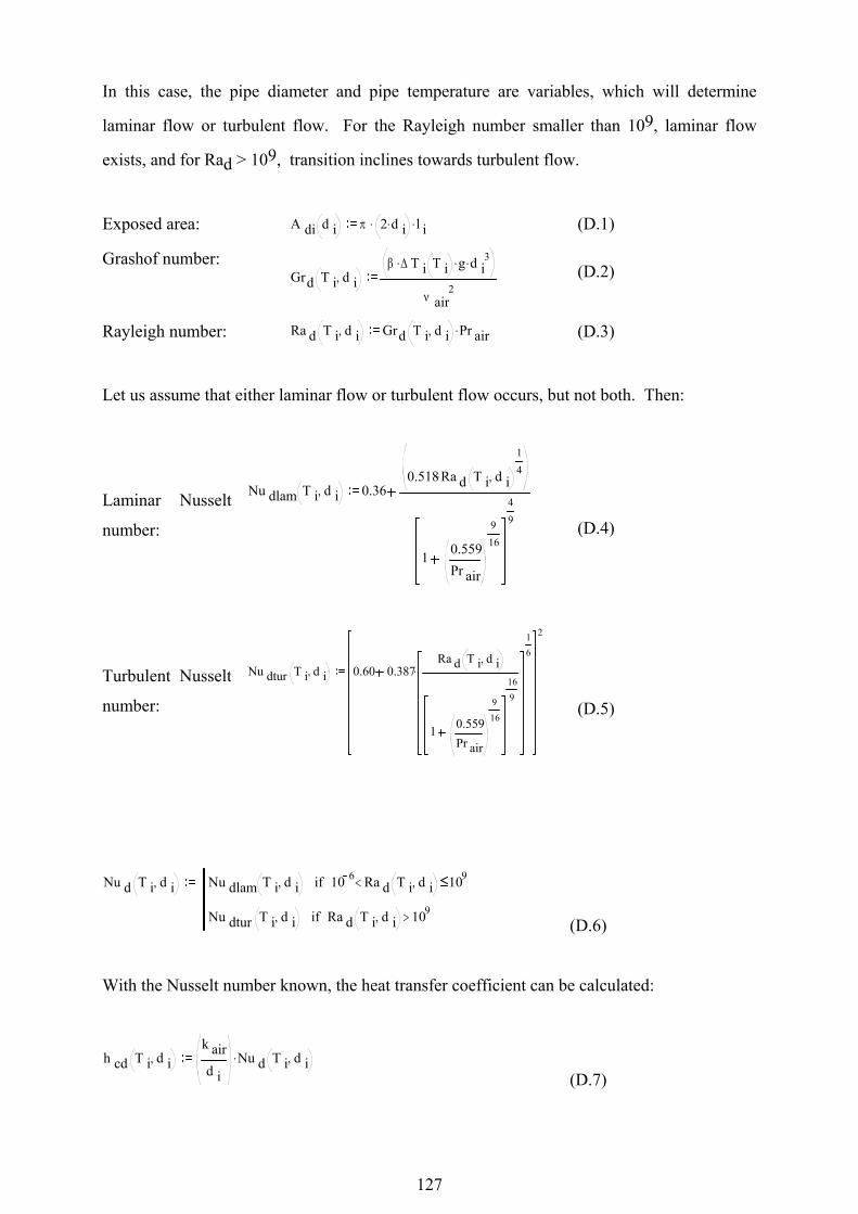
127

In this case, the pipe diameter and pipe temperature are variables, which will determine

laminar flow or turbulent flow. For the Rayleigh number smaller than 109, laminar flow

exists, and for Rad > 109, transition inclines towards turbulent flow.

Exposed area: A di d i π 2 d i.. l i. (D.1)

Grashof number: Grd T i d i,

β Δ T i T i. g. d i3.

ν air2

(D.2)

Rayleigh number: Ra d T i d i, Grd T i d i, Pr air. (D.3)

Let us assume that either laminar flow or turbulent flow occurs, but not both. Then:

Laminar Nusselt

number:

Nu dlam T i d i, 0.360.518 Ra d T i d i,

14.

1 0.559Pr air

916

49

(D.4)

Turbulent Nusselt

number:

Nu dtur T i d i, 0.60 0.387Ra d T i d i,

1 0.559Pr air

916

169

16

.

2

(D.5)

Nu d T i d i, Nu dlam T i d i, 10 6 Ra d T i d i,< 109if

Nu dtur T i d i, Ra d T i d i, 109>if (D.6)

With the Nusselt number known, the heat transfer coefficient can be calculated:

h cd T i d i,k aird i

Nu d T i d i,.

(D.7)

128

Then, the heat loss is calculated as follows:

Q dloss T i d i, h cd T i d i, A di d i. Δ T i T i. (D.8)

D.1.2 Natural Convection over Vertical Wall

For a vertical cylinder with natural convection, one can approximate the cylinder as a vertical

wall:

Exposed area: A Li d i π 2 d i.. l i. (D.9)

Grashof number:

x 0.1 m

GrL T iβ Δ T i T i. g. l i

3.

ν air2

(D.10)

Rayleigh number: Ra L T i GrL T i Pr air. (D.11)

Transition from laminar to turbulent flow will occur at Grx~109 with the Prandtl number

function:

Ψ 1 0.492Pr air

916

169

(D.12)

with

Ψ 0.343=

Laminar Nusselt

number:

Nu Llam T i 0.68 0.67 Ra L T i Ψ.

14.

(D.13)

Turbulent

Nusselt number:

Nu Ltur T i 0.68 0.67 Ra L T i Ψ.

14. 1 1.6 10 8. Ra L T i. Ψ.

112

.

129

(D.14)

The Nusselt number is:

Nu L T i Nu Llam T i Ra L T i 109if

Nu Ltur T i 109 Ra L T i< 1012<if (D.15)

with the heat transfer coefficient reflected by:

h cL T ik airl i

Nu L T i.

(D.16)

and the heat loss to the environment:

Q Lloss T i d i, h cL T i A Li d i. Δ T i T i. (D.17)

For a typical pipe of 50 mm diameter and with 8 bar steam pressure, or an equivalent of

443.5 K (170.2 oC), the energy loss for 1 m of unlagged piping is:

Q dloss 443.5 K 0.05 m,( ) 386.864W= (D.18)

Q Lloss 443.5 K 0.05 m,( ) 343.09W= (D.19)

Q 370K d i,

Q 425K d i,

Q 480K d i,

d i

0 0.02 0.04 0.06 0.08 0.1 0.12 0.14 0.16 0.18 0.20

1000

2000

Figure D. 1: Convection heat loss: variable pipe diameter

130

From figure D.1 it is clear that convection heat loss is directly proportional to pipe diameter at

constant temperatures.

D.1.3 Effect of Radiation on Energy Losses for Unlagged Steam Pipes

The stainless-steel piping will be subject to solar and sky irradiation. The solar radiation

absorptance for stainless steel (Mills, 1995) and the hemispherical emmitance and reflectivity

are given in the table below:

.

Absorptivity for stainless steel α ss 0.89

Hemispherical emittance ε s 0.20

Reflectivity ρ s 1 α ss

Stefan-Boltzmann constant σ 5.670 10 8. W

m2 K4.

Table D. 2: Radiation properties of stainless steel (Mills, 1995)

Calculating the Emmissivity of the Sky

For a dry-bulb temperature of 288.15 K (15 oC) and a wet-bulb temperature of 286.55 K (13.4 oC), the relative humidity is 85% from the psychrometric chart, and the saturated vapour

pressure at 288.15 K is 1704.4 Pa. Therefore, the partial pressure of water vapour is:

P vapour 0.85 1704.4Pa.

(D.20)

with atmospheric pressure:

P atm 101300Pa (D.21)

According to Mills, 1995, the sky emissivity is:

ε sky 0.55 1.8P vapour

P atm

12

.

(D.22)

ε sky 0.765=

131

Therefore, sky irradiation is:

Gsky ε sky σ. T dbplant4. (D.23)

The total radiation heat flux is represented by the following:

q radpipe T i ε s σ. T i4. ρ s Gsky. α ss Gsky.

(D.24)

With total radiation heat transfer:

Q rad T i d i, q radpipe T i A di d i.

(D.25)

Radiative heat transfer per 1 m length of steam pipe at 0.8 MPa (8 bar) absolute pressure and

with a 50 mm outside pipe diameter:

Q rad 443.5 K 0.05 m,( ) 64.527W=

QradTi 0.05m,

Ti

360 380 400 420 440 460 4800

50

100

150

Figure D. 2: Radiation heat loss: variable temperature

From figure D.2, it is evident that an exponential relationship exists between radiation heat

loss and surface temperature.

Total Heat Transfer – Radiative and Convective – for Steam Pipe of 1 m Length

Because most steam pipes are placed horizontally, it is only necessary to look at horizontal

steam pipes.

132

Q total T i d i, Q dloss T i d i, Q rad T i d i, (D.26)

For a horizontal steam pipe at 8 bar steam pressure and with a diameter of 50 mm, the heat

loss per meter is:

Q total 443.5 K 0.05 m,( ) 451.391W= (D.27)

Cost of Steam Generated from Coal

Consider a coal price of R447 per ton. The calorific value of A-grade pea coal is 28.5 MJ/kg.

For 1 W of steam saved at a utilisation point, ignoring inefficiencies (except boiler

efficiency), the amount of coal that is used will be:

Boiler efficiency: η boiler 0.85 (D.28)

Calorific value of pea coal: Cal pea 28.5 106. Jkg

(D.29)

Usage rate1 W( )

Cal pea η boiler. Usage rate 4.128 10 8. kg

s= (D.30)

Coal price0.447

kg (D.31)

Cost rate Usage rate Coal price.

Cost rate 1.845 10 8. Hz=

(D.32)

Cost of 1 m of Unlagged Piping

Once again, a typical pipe will be used to indicate losses. The cost will be evaluated on a

period of one year:

Yearlycost 300 dayCost rate

W. Q total 443.5 K 0.05 m,( ).

(D.33)

Yearlycost 215.89= (D.34)

133

Thus, for 1 m of steam pipe (8 bar, 0.05 m diameter) that is exposed to the plant environment,

it will cost a plant an additional R215.89 per annum for energy consumption.

Percentage Analysis of Heat Transfer Losses from Unlagged Steam Pipes

Comparisons of radiative heat transfer to convective heat transfer, as well as between vertical

and horizontal piping, are indicated below.

Horizontal-to-vertical ratio:

Q dloss 443.5 K 0.05 m,( )

Q Lloss 443.5 K 0.05 m,( )1.128=

(D.35)

Radiative-to-convective heat transfer ratio for horizontal piping:

Q rad 443.15K 0.05 m,( )

Q rad 443.5 K 0.05 m,( ) Q dloss 443.5 K 0.05 m,( )0.142=

(D.36)

Conclusions

From the above calculations, the following conclusions can be drawn:

1. The heat loss for vertical and horizontal piping is almost the same, although horizontal

piping has more convective heat loss to the environment.

2. For an unlagged steam pipe of 1 m and with an outside diameter of 50 mm and 0.8

MPa (8 bar) absolute saturated steam pressure, assuming the temperature on the

outside is almost the steam temperature, radiative heat loss is ± 14% of the total heat

loss of 451.391 W and the cost of the heat loss is equivalent to R215.89 per annum.

134

E APPENDIX: HEAT LOAD CALCULATIONS FOR INSULATION PANELS

135

E.1 Calculation of Heat Load on Outside Panels of Cooling Room

Heat on the outside panel is transferred through radiation and convection. By measuring the

dry and wet-bulb temperature and assuming correlations for irradiation on the panel during

different times of the day, recognising the direction to which the perpendicular on the panel

points, it is possible to estimate the amount of heat that travels through the insulation into the

cooling room.

Geometry of insulation panel:

L wall 7 m W wall 7 m A wall L wall W wall.

Table E. 1: Dimensional properties of insulation panel

Temperature measurements and atmospheric conditions:

T dbo 287.15K Twbo 286.75K

P atm 101325Pa u wind 0.2 ms

T po 284.75K T dbi 253.15K RH i 0.56 T pi 255.15K

Table E. 2: Temperature measurements and atmospheric conditions

Radiation properties:

ε p 0.85 α p 0.25

Table E. 3: Radiation properties of insulation panel

Assume an average relative humidity of 83%:

RH 0.83 (E.1)

Correlation for determining saturated vapour pressure in the cooling room:

136

C 1 5.6745359103. C 2 5.152305810 1.

C 3 9.677843010 3. C 4 6.221570110 7.

C 5 2.074782510 9. C 6 9.484024010 13.

C 7 4.1635019 C 8 5.8002206103.

C 9 5.516256100. C 10 4.864023910 2.

C 11 4.176476810 5. C 12 1.445209310 8.

C 13 6.5459673

Table E. 4: Coefficients for calculation of saturated vapour pressure

P vsat T( ) 1000 e

C 8 K.

TC 9 C 10

TK

. C 11T2

K2. C 12

T3

K3. C 13 ln

TK

.

Pa.. (E.2)

Using perfect gas relations for the dry and moist air,

P vsat T dbo 1.599 103. Pa= (E.3)

from equations E.1 and E.2, the vapour pressure is obtained:

P v RH P vsat T dbo.

(E.4)

P v 1.327 103. Pa=

From a correlation in Mills, 1995, the sky emissivity is:

ε sky 0.55 1.8P v

P atm.

(E.5)

ε sky 0.574=

Properties of air:

density:

137

ρ air T( )P atm

287.08 Jkg K.

T. (E.6)

ρ air T dbo 1.229 kg

m3=

dynamic viscosity:

μ air T( ) 2.28797310 6. 6.25979310 8. TK

. 3.13195610 11. TK

2. 8.1503810 15. T

K

3. kg

s m.

(E.7)

kinematic viscosity:

ν air T( )μ air T( )

ρ air T( ) (E.8)

thermal conductivity:

k air T( ) 4.93778710 4. 1.01808710 4. TK

. 4.62793710 8. TK

2. 1.25060310 11. T

K

3. W

m K.

(E.9)

specific heat:

c pair T( ) 1.045356103. 3.16178310 1. TK

. 7.08381410 4. TK

2. 2.70520910 7. T

K

3. J

kg K.

(E.10)

Prandtl number: Pr T( )c pair T( ) μ air T( ).

k air T( ) (E.11)

Prandtl number function: Ψ T( ) 1 0.492

Pr T( )

916

169

(E.12)

Volumetric expansion

coefficient:

βρ air T pi ρ air T dbo

ρ air T pi T pi T dbo.

(E.13)

β 3.483 10 3. 1K

=

Grashof number:

x 1 m

Grx x( )β T pi T dbo. g. x3.

ν air T dbo2

(E.14)

138

GrL Grx L wall

(E.15)

Rayleigh number: Ra L T dbo GrL Pr T dbo. (E.16)

Reynolds number:

Re x x( )

u wind x.

ν air T dbo (E.17)

There are two scenarios for convection heat transfer: natural convection and forced

convection, with an assumed average wind speed. Calculations are done for both.

Natural Convection (Laminar and Turbulent Flow)

Point of transition for natural convection:

root Grx x( ) 109 x, 0.578 m=

x tr root Grx x( ) 109 x,

Laminar Nusselt number:

Nu Lnatlam 0.68 0.670 Ra L T dbo Ψ T dbo.

14. (E.18)

Turbulent Nusselt number:

Nu Lnattur 0.68 0.670 Ra L T dbo Ψ T dbo.

14. 1 1.6 10 8. Ra L T dbo. Ψ T dbo.

112

.

(E.19)

Nu Lnatural Nu Lnatlam Ra L T dbo 109if

Nu Lnattur 109 Ra L T dbo< 1012if (E.20)

Because the wall is 7 m high, for the sake of simplicity, we ignore the laminar part and

assume turbulent flow for the full height of the wall.

139

Forced Convection (Laminar and Turbulent Flow)

For plate flow, there will always be a laminar and turbulent region due to the length of the

plate. The point of transition can be solved with the root function.

Re trans 50000 (E.21)

x trturb root Re x x( ) Re trans x, x trturb 3.635 m= (E.22)

Average Nusselt number:

Nu Lforced 0.664 Re x xtrturb

12. Pr T dbo

13. 0.036 Re x L wall

0.8. Pr T dbo0.43. 1

Re x xtrturbRe x L wall

0.8

.

(E.23)

Nusselt number:

Nu L Nu Lnatural u wind 0 ms

if

Nu Lforced u wind 0 ms

>if (E.24)

Convection heat transfer coefficient:

h convk air T dbo Nu L.

L wall (E.25)

h conv 0.922 kg

s3 K.=

Heat transfer due to convection:

q conv h conv T dbo T po.

(E.26)

q conv 2.213 kg

s3=

140

Radiation Heat Transfer

Radiation heat transfer comprises solar irradiation, sky irradiation and emission from the

surface. The solar irradiation, Gs, is a function of the time of day and year.

Gs 19 W

m2 (E.27)

q rad α p ε sky. σ. T dbo4. α p G s. ε p σ. T po

4. T po T dbo>if

α p ε sky. σ. T dbo4. α p G s. T po T dboif

(E.28)

q rad 60.024 kg

s3=

Overall Heat Gain from Atmosphere Next to Panel

q total q conv q rad (E.29)

q total 62.237 kg

s3=

With the overall heat gain calculated, it is possible to determine the overall heat transfer

coefficient, Uactual, by dividing qtotal by the temperature difference,

Tpo - Tpi:

U actualq total

T po T pi (E.30)

U actual 2.103 kg

s3 K.=

141

Calculation of Design Value for Insulation

The insulation consists of polystyrene foam with steel plates on both sides, coated with white

paint. The steel plates are glued to the polystyrene foam, but for the sake of simplicity, we

will ignore the effect of the paint and the glue on the heat transfer coefficient of the insulation

panel.

Thickness of steel plates t s 0.0015m

Thickness of polystyrene t p 0.150 m

Thermal conductivity of steel k s 15 Wm K.

Thermal conductivity of polystyrene k p 0.04 Wm K.

Table E. 5: Properties of insulation panel

The design value of the overall heat transfer coefficient is as follows:

U designt pk p

2 t s.

k s

1

(E.31) U design 0.267 kg

s3 K.=

For the panels on the eastern side of cold stores 1 and 3, an extra layer of panels of 50 mm is

added:

t pextra 200 mm (E.32)

Replacing ts in equation (E.31) with tpextra in equation (E.32), the overall heat transfer

coefficient for the southern wall is obtained:

U designsouth4 t s.

k s

t pextrak p

1

(E.33)

U designsouth 0.2 kg

s3 K.=

142

Comparison of the design value and the actual values:

PercentageU actual

U designsouth (E.34)

Percentage 10.514=

This means that if the inside temperature is -18 oC and the outside temperature is the same as

the environment temperature at night (14 oC), then:

Q total U designsouth T po T pi.

(E.35)

Q total 5.92 kg

s3=

The percentage improvement, assuming that new insulation panels are performing at design

values, is as follows:

Improvementq total Q total 100.

Q total (E.36)

Improvement 951.382=

Thus, the insulation effect will be improved by 951% if new insulation is installed.

143

F APPENDIX: COLD STORE CALCULATIONS

144

F.1 Cold Store Calculations

The purpose of the calculations is to determine the effect of water vapour on air that enters the

cooling rooms through infiltration effects and which is condensed and frozen in the cold

stores, as well as heat loss through poor insulation.

F.1.1 Infiltration Effect

1) The specific humidity of the passage and cooling room must be calculated.

2) The potential for mass transfer can now be used to determine infiltration.

TCOOL

Environment

Cooling roomPassage

Heat exchanger and Fan

Important to determine the effect of poor insulation on the heat load of the refrigeration by measuringsurface temperatures all around the cooling room and calculating the conduction coefficient of each sideand determining the loss to the environment.Temperatures on the in and outsides must be compared with design specifications to determine costsavings possible.To determine the refrigeration load, one can measure the mass flow of the refrigerant in the heatexchanger and the inlet and outlet temperatures and pressures, or the air flow across the heat exchangercan be determined and the inlet and outlet wet and dry bulb temperatures can be measured.The question is whether or not all these abovementioned equipment is really neccessary. Is it possible todetermine mass flowrate at the outlet of the compressor ?

Refrigeration load

Hot humid air

Cold dry air

Infiltratio

Figure F. 1: Schematic representation of heat transfer of cold store

T dbc 248.15K T evap 236.15K T dbp 287.113K T nbp 286.152K

145

P atm 101325Pa

Table F. 1: Plant and cold store conditions

Correlation for determining vapour pressure in the cooling room:

C 1 5.6745359103. C 2 5.152305810 1.

C 3 9.677843010 3. C 4 6.221570110 7.

C 5 2.074782510 9. C 6 9.484024010 13.

C 7 4.1635019 C 8 5.8002206103.

C 9 5.516256100. C 10 4.864023910 2.

C 11 4.176476810 5. C 12 1.445209310 8.

C 13 6.5459673

Table F. 2: Constants for saturated vapour pressure

The vapour pressure can be calculated from the following correlations (Kröger, 1998):

P vicesat T( ) 1000 e

C 1 K.

TC 2 C 3

TK

. C 4T2

K2. C 5

T3

K3. C 6

T4

K4. C 7 ln

TK

.

Pa..

(F.1)

P vliqsat T( ) 1000 e

C 8 K.

TC 9 C 10

TK

. C 11T2

K2. C 12

T3

K3. C 13 ln

TK

.

Pa..

(F.2)

Using perfect gas relations for the dry and moist air,

P vsat T( ) P vicesat T( ) T 273.15Kif

P vliqsat T( ) T 273.15K>if (F.3)

cold store vapour pressure is obtained by applying equations F.1, F.2 and F.3 for Tdbc:

146

P vcsat P vsat T dbc (F.4) P vcsat 63.289Pa=

The passage vapour pressure is obtained in the same way as above, but for Tdbp.

P vpsat P vsat T dbp (F.5)

P vpsat 1.595 103. Pa=

With the saturation vapour pressure known for the cooling room and the passage, the

saturated specific humidity can be found respectively

ω csat0.62198P vcsat.

P atm P vcsat (F.6)

ω csat 3.887 10 4.=

ω psat0.62198P vpsat.

P atm P vpsat (F.7)

ω psat 9.946 10 3.=

The specific heat capacity for dry air:

c pa 1006 Jkg K. (F.8)

Calculation of Relative Humidity in Cold Store

Assuming that the dew-point temperature of the cold store approximates the evaporator

surface temperature, Tevap, the vapour pressure in the cold store can be approximated and,

therefore, the wet-bulb temperature can be calculated. Constants from ASHRAE

Fundamentals (1993), used to calculate the dew-point temperature of liquid and ice:

147

C 14 6.54 C 15 14.526 C 16 0.7389 C 17 0.09486 C 18 0.4569

Table F. 3: Constants to determine dew-point temperature

A first value is selected as Pvcroot from where MathCAD starts an iterative process to

determine the true vapour pressure Pvc, setting the dew-point temperature equal to the

evaporator temperature:

P vcroot P vcsat 0.5.

(F.9)

T dice P vcroot 6.09 12.608lnP vcroot1000 Pa

. 0.4959 lnP vcroot1000 Pa

2

. 273.15 K

(F.10)

T dliq P vcroot C 14 C 15 lnP vcroot1000 Pa

. C 16 lnP vcroot1000 Pa

2

. C 17 lnP vcroot1000 Pa

3

. C 18P vcroot1000 Pa

0.1984

. 273.15 K

(F.11)

T dew P vcroot T dice P vcroot T dbc 273.15K<if

T dliq P vcroot T dbc 273.15Kif (F.12)

root T dew P vcroot T evap P vcroot, 17.097Pa= (F.13)

P vc root T dew P vcroot T evap P vcroot, (F.14)

thus,

RH cP vc

P vcsat (F.15) RH c 0.27=

148

Determining the specific humidity:

ω c0.62198P vc.

P atm P vc (F.16)

ω c 1.05 10 4.=

The conservation of energy in adiabatic saturation of air at a known dry-bulb temperature and

relative humidity is applied. Specific enthalpy for dry air:

h a T( ) c pa T 273.15K( ).

(F.17)

The specific enthalpy for water vapour is demonstrated by:

h v T( ) 2501 103. 1805 T 273.15K( )K

. Jkg (F.18)

The specific enthalpy for ice and water liquid respectively:

h fice T( ) 1888.27 TK

. 849.88103. Jkg (F.19)

h fliq T( ) 4183.9 TK

. 1142.7103. Jkg (F.20)

For temperatures above 273.15 K equation F.20 is used, otherwise F.19 is used:

h f T( ) h fice T( ) T 273.15Kif

h fliq T( ) T 273.15K>if (F.21)

The specific enthalpy for evaporation is shown below:

149

h fg T( ) 1000 0.0038 TK

2. 1.8164 T

K. 2621.9. J

kgT 273.15Kif

1000 3151.5 2.3814 TK

.. Jkg

T 273.15K>if (F.22)

The specific enthalpy values for dry air and water vapour are as follows:

h a1 h a T dbc h a1 2.515 104. Sv= h v1 h v T dbc h v1 2.456 106. Sv=

Table F. 4: Specific enthalpy values for dry air and water vapour

Calculation of Wet-bulb Temperature in Cold Store

For calculation purposes in MathCAD, a value for the wet-bulb temperature was guessed,

which was substituted into equation (F.23) and changed to find the roots of the equation, in

order to find the actual wet-bulb temperature.

T nbcroot 200 K ω csat T nbcroot0.62198P vsat T nbcroot.

P atm P vsat T nbcroot

h a2 T nbcroot h a T nbcroot h v2 T nbcroot h v T nbcroot h f2 T nbcroot h f T nbcroot h fg2 T nbcroot h fg T nbcroot

Table F. 5: Equations to determine wet-bulb temperature

f c T nbcroot ω c ω csat T nbcroot h f2 T nbcroot. h a2 T nbcroot ω csat T nbcroot h v2 T nbcroot. h a1 ω c h v1.

(F.23) root f c T nbcroot T nbcroot, 247.427K= (F.24)

From equation (F.24) we have the wet-bulb temperature, and equation (F.25) represents the

wet-bulb temperature of the cold store:

T nbc root f c T nbcroot T nbcroot, (F.25) T nbc 247.427K=

150

Calculation of Specific Humidity of Passage Air

h a1 h a T dbp

h a2 h a T nbp

h a1 1.405 104. Sv=

h a2 1.308 104. Sv= h v1 h v T dbp h v1 2.526 106. Sv= h v2 h v T nbp h v2 2.524 106. Sv= h f2 h f T nbp h f2 5.453 104. Sv= h fg2 h fg T nbp

ω pnsat0.62198P vsat T nbp.

P atm P vsat T nbp ω pnsat 9.333 10 3.=

ω ph a2 h a1 ω pnsat h fg2.

h v1 h f2 ω p 8.936 10 3.=

RH pω p

ω psat RH p 0.898=

Table F. 6: Calculation of specific and relative humidity of passage air

Partial Pressure of Water Vapour

The partial pressure of the water vapour in the cold store is:

P vcP atm ω c.

0.62198 ω c (F.26) P vc 17.097Pa=

and the partial pressure of water vapour in the passage is:

P vpP atm ω p.

0.62198 ω p (F.27)

P vp 1.435 103. Pa=

The enormous difference between the vapour pressure of the cold store and that of the passage

is the driving force behind vapour transfer into the cold store.

151

F.1.2 Mass Transfer

With the specific humidities of the cold store and the passage known, the mass transfer of

water vapour from the passage to the cold store can be determined. Approach the problem as

the diffusion of one gas through a second stagnant gas (ASHRAE Fundamentals Handbook,

1993).

Fick’s law for ideal gases with negligible pressure gradient states the following:

J B ρ D ν.

y

ρ Bρ

dd

.

(F.28)

J BC C D ν.

y

C BC

dd

. (F.29)

This is the basic equation for molecular diffusion, expressing the concentration of component

B of a binary mixture in terms of the mass fraction (ρΒ/ρ) or mole fraction (CB/C). Dν, the

proportionality factor, is the mass diffusivity or the diffusion coefficient. The diffusive mass

flux and diffusive molar flux are:

J B ρ B ν B ν. and J BC C B ν B ν.

where ν B ν is the velocity of component B relative to the mixture velocity. Remember

that C Bρ BM B

, and thus all results can be converted to the molar form and otherwise. Let’s

look at the physical situation we have here:

152

TCOOLCooling roomTdbcTnbcRHc

PassageTdbpTnbpRHp

Hot humid air

Cold dry air

Infiltration effect

Figure F. 2: Schematic drawing of vapour transfer phenomena

The difference between concentration of water vapour in the cold store, CBCool, and

concentration of water vapour in the passage, CBPass, will result in a net mass flux of vapour

into the cold store, resulting in additional cooling load requirements. Fick’s law on the cold

store and the passage states:

J Bc ρ c D νc.y

ρ Bcρ c

dd

.

(F.30)

J Bp ρ p D νp.y

ρ Bpρ p

dd

.

(F.31)

from

ωm Bm a (F.32)

and

m t m B m a (F.33)

153

also, then ρ ρ B ρ a and in a fixed volume we have ρ B

ρ

m Bm t

=

and deviding above and under by ma, we have m Bm t

ω

ω 1= .

Therefore, the mass flux can be calculated in terms of specific humidity.

J Bnet ρ c D νc.y

ρ Bcρ c

dd

. ρ p D νp.y

ρ Bpρ p

dd

.

(F.34)

J Bnet ρ c D νc.y

ω cω c 1

dd

. ρ p D νp.y

ω pω p 1

dd

.

(F.35)

The different densities of the cold store and the passage can be determined with the known

dry-bulb and wet-bulb temperatures, where the calculation of the diffusion coefficient will

follow.

Calculation of the Diffusion Coefficient

An empirical equation for the mass diffusivity of water vapour in air (ASHRAE

Fundamentals Handbook, 1993) is as follows:

D ν0.926

pT2.5

T 245.

(F.36)

Density calculations for moist air in the cold store and passage provided the following results:

ρ c 1 ω c 1ω c

ω c 0.62198.

P atm

287.08 Jkg K.

. T dbc.

.

(F.37)

ρ c 1.422 kg

m3=

154

ρ p 1 ω p 1ω p

ω p 0.62198.

P atm

287.08 Jkg K.

. T dbp.

.

(F.38)

ρ p 1.223 kg

m3=

The diffusion coefficient for the air in the cold store and passage is given by:

D νc0.926

1000 P atm.

T dbc2.5

T dbc 245 Kkg. m.

K1.5 s3..

(F.39)

D νc 1.798 10 5. m2

s=

D νp0.926

1000 P atm.

T dbp2.5

T dbp 245 Kkg. m.

K1.5 s3..

(F.40)

D νp 2.399 10 5. m2

s=

Approximating dy as very small, for example d y 0.001 m, the net mass flux JBnet can be

calculated:

J Bnet ρ c D νc.

ω cω c 1

d y. ρ p D νp.

ω pω p 1

d y.

(F.41) J Bnet 2.571 10

4 . kg m

2 s .

=

Therefore, the daily mass transfer of water vapour from the passage through the door to the

cold store, with the assumption that the door is effectively open for three hours each day, is:

m transfer J Bnet A door. t open.

(F.42) m transfer 20.16 kg=

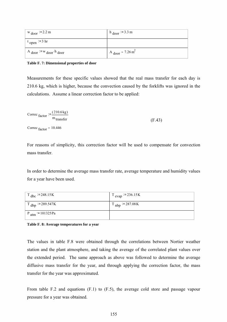
155

w door 2.2 m h door 3.3 m t open 3 hr

A door w door h door. A door 7.26 m2=

Table F. 7: Dimensional properties of door

Measurements for these specific values showed that the real mass transfer for each day is

210.6 kg, which is higher, because the convection caused by the forklifts was ignored in the

calculations. Assume a linear correction factor to be applied:

Correc factor210.6 kg( )

m transfer (F.43) Correc factor 10.446=

For reasons of simplicity, this correction factor will be used to compensate for convection

mass transfer.

In order to determine the average mass transfer rate, average temperature and humidity values

for a year have been used.

T dbc 248.15K T evap 236.15K T dbp 289.547K T nbp 287.08K P atm 101325Pa

Table F. 8: Average temperatures for a year

The values in table F.8 were obtained through the correlations between Nortier weather

station and the plant atmosphere, and taking the average of the correlated plant values over

the extended period. The same approach as above was followed to determine the average

diffusive mass transfer for the year, and through applying the correction factor, the mass

transfer for the year was approximated.

From table F.2 and equations (F.1) to (F.5), the average cold store and passage vapour

pressure for a year was obtained.

156

The cold store vapour pressure is:

P vcsat P vsat T dbc (F.44) P vcsat 63.289Pa=

The passage vapour pressure is:

P vpsat P vsat T dbp (F.45)

P vpsat 1.865 103. Pa=

With the saturation vapour pressure known for cold store and the passage, the saturated

specific humidity can be found:

ω csat0.62198P vcsat.

P atm P vcsat (F.46)

ω csat 3.887 10 4.=

ω psat0.62198P vpsat.

P atm P vpsat (F.47)

ω psat 0.012=

From equation (F.15), the relative humidity and the specific humidity of the cold store is

known.

Conservation of energy in adiabatic saturation of air at a known dry-bulb temperature and

relative humidity was applied by using equations (F.17) to (F.22).

The cold store wet-bulb temperature remains the same, and therefore the enthalpies remain

the same.

157

Calculation of Specific Humidity of Passage Air

h a1 h a T dbp

h a1 1.65 104. Sv=

h a2 h a T nbp

h a2 1.401 104. Sv=

h v1 h v T dbp h v1 2.531 106. Sv= h v2 h v T nbp h v2 2.526 106. Sv= h f2 h f T nbp h f2 5.841 104. Sv= h fg2 h fg T nbp

ω pnsat0.62198P vsat T nbp.

P atm P vsat T nbp ω pnsat 9.925 10 3.=

ω ph a2 h a1 ω pnsat h fg2.

h v1 h f2 ω p 8.903 10 3.=

RH pω p

ω psat

RH p 0.763=

Table F. 9: Calculation of specific and relative humidity of passage air

Partial pressure of water vapour for the cold store and passage respectively:

P vcP atm ω c.

0.62198 ω c (F.48) P vc 17.097Pa=

P vpP atm ω p.

0.62198 ω p (F.49)

P vp 1.43 103. Pa=

158

Mass Transfer

Thus, the mass flux can be calculated in terms of specific humidity as before.

J Bnet ρ c D νc.y

ω cω c 1

dd

. ρ p D νp.y

ω pω p 1

dd

.

The different densities of the cooling room and the passage can be determined with the known

dry-bulb and wet-bulb temperatures, upon which the calculation of the diffusion coefficient

will follow. An empirical equation for the mass diffusivity of water vapour in air (ASHRAE,

1993) is as follows:

D ν0.926

pT2.5

T 245.

Density calculations for moist air in passage:

ρ p 1 ω p 1ω p

ω p 0.62198.

P atm

287.08 Jkg K.

. T dbp.

.

(F.50)

ρ p 1.212 kg

m3=

Diffusion coefficient for passage:

D νp0.926

1000 P atm.

T dbp2.5

T dbp 245 Kkg. m.

K1.5 s3..

(F.51)

D νp 2.439 10 5. m2

s=

The net mass flux from equation (F.41) is:

smkgJ Bnet ⋅

⋅= −2

410583.2 (F.52)

159

Thus, the daily mass transfer of water vapour from the passage through the door to the cold

store, with the assumption that the door is effectively open for three hours each day, is, for

average values:

m transfer 20.252kg= (F.53)

Therefore, the average vapour transfer rate for infiltration alone is 20.252 kg.

Energy transfer due to different states of water vapour:

Water vapour gas constant R v 461.5 Jkg K. (F.54)

Critical pressure P cr 22.09 106 Pa. (F.55)

Critical temperature T cr 647.3 K (F.56)

Specific volume of vapour in cold store:

υ cR v T dbc.

P vc υ c 6.698 103. m3

kg= (F.57)

Specific volume of vapour in passage:

υ pR v T dbp.

P vp υ p 92.326 m3

kg= (F.58)

The internal energy change of water vapour is:

Δ u v aT dbp

K

T dbcK

. b2

T dbpK

2 T dbcK

2

. a 1

υ ckg

m3.

1

υ pkg

m3.

. Jkg

(F.59)

Δ u v 6.644 104. Sv=

where

160

a27 R v

2. T cr2. kg. s2.

64 P cr. m5.

a 1.704 103.= (F.60)

and

b

R v T cr. kg.

8 P cr. m3.

b 1.69 10 3.= (F.61)

The specific enthalpy change of water vapour is given by:

Δ h v Δ u v P vp υ p. P vc υ c. (F.62)

Δ h v 8.442 104. Sv=

The energy needed to freeze 1 kg of water vapour is:

E freeze 2.061 106. Jkg (F.63)

Enthalpy Increase in Cold Store

The enthalpy increase is given by:

E freeze Δ h v 2.145 106. Sv= (F.64)

The mass of water that is condensed and frozen per day is as follows:

m peryear 400 kg (F.65)

The average enthalpy increase per day is:

H experimental m peryear Δ h v E freeze. (F.66)

The average enthalpy increase for one year is:

161

H experimentalperyear H experimental365

kW hr..

(F.67)

H experimentalperyear 8.701 104.=

In Rand-value, the energy cost just for removing moisture from the air is approximately

R0,15:

Unit 0.15 (F.68)

Cost Unit H experimentalperyear.

(F.69)

Cost 1.305 104.=

Thus, the extra energy cost due to water vapour infiltration amounts to R13 050 per year.

162

G APPENDIX: PAYBACK CALCULATIONS FOR AIR CURTAINS FOR COLD STORES

163

G.1 Payback Calculations of Air Curtains for the Cold Stores

Calculations are done to establish the amount that can be saved annually in terms of energy

costs when the vapour transfer into the cold store is reduced by 80%. Maintenance costs are

approximated as 10% of the capital costs for the first two years and thereafter 20%. Each unit

uses 2.2 kW electrical energy to drive the fan motor and costs R4 950. The average unit

price, assuming the operating time of the air curtains are spread evenly throughout the day, is

19 c. The average amount of water vapour condensed onto the evaporators is approximated at

211.55 kg per day, thus:

m freeze 211.52kg (G.1)

With an effectiveness of 80% in limiting vapour transfer to the cold store, the mass of water

vapour kept from infiltrating the cold store is:

η eff 0.8 (G.2)

m saved η eff m freeze. (G.3)

m saved 169.216kg=

Assume the plant is operative for 350 days of the year, then the water that would have been

condensed amounts to: 169.216 kg x 350 = 59234.67 kg. The energy value to condense

vapour and freeze it to the temperature of the evaporator, Tevap, is:

e freeze 2947000 Jkg (G.4)

The energy saved for one year is then: E year e freeze m saved. 350.

(G.5)

E year 1.745 1011. J=

164

The amount of kWh saved for the year is as follows:

Amount kWhE yearkW hr. (G.6)

Amount kWh 4.848 104.=

Assume the average cost for 1 unit (1 kWh) is 19 c, then the infiltration cost will be:

Cost infiltration 0.19 Amount kWh.

(G.7)

Cost infiltration 9.212 103.=

For two air curtains, the total capital cost is:

Cost aircurtains 2 4950.

(G.8)

The maintenance cost for two air curtains is:

Cost maintenance 0.1 Cost aircurtains.

(G.9)

Assume that the air curtains operate full-day, then the annual running cost of the air curtains

will be:

Cost electricity0.17 2.2. kW 24. hr 300.( )

kW hr. (G.10)

The total running cost for each year for the first two years is the sum of equations (G.7) to

(G.10), thus:

Cost running Cost maintenance Cost electricity (G.11)

Cost running 3.683 103.=

The potential savings are determined by subtracting equation (G.11) from equation (G.7):

165

Cost savings Cost infiltration Cost running (G.12)

Cost savings 5.529 103.=

A simple payback calculation gives:

n yearCost aircurtains

Cost savings (G.13) n year 1.791=

Thus, in almost two years’ time the air curtains would have paid for themselves. In addition,

the safety factor of visibility, which as always has a financial risk attached to it, should be

taken into consideration.

166

H APPENDIX: INVESTIGATION OF IMPROVEMENT OF STEAM UTILISATION

167

H.1 Investigation of Improvement of Steam Utilisation

The steam peeler uses steam to peel potatoes and then discards the steam into the atmosphere.

This investigation will look into the possibility of utilising the steam for the blanchers or hot

water.

H.1.1 Steam Peeler

Steam consumption at a production rate of 1 000 kg potatoes per hour requires 100 kg

saturated steam at 1.6 MPa (16 bar) absolute pressure. Thus, for a current production rate of

100 t (100 000 kg) French fries per day, with an availability of 97% and 22 hours of

production, the incoming product mass flow rate (equation (H.4)) is calculated:

Prod rate 100 tonday (H.1)

availability 0.97 (H.2)

yield 0.5 (H.3)

Prod raw Prod rate 24. hrday

availabilityyield

. (H.4)

Prod raw 2.037 kgs

=

The amount of steam used is as follows:

steam used 0.1 kgProd raw

1 kg.

(H.5)

steam used 0.204 kgs

=

To determine the energy content of the steam that is discarded, one can approximate it with

the design calculations of a Dutch company, Uticon-Dynatherm Industrie bv. By knowing the

168

mass loss of the potatoes in the steam peeler, the steam that is used can be approximated. Due

to the short time of exposure, it can be assumed that very little sensible heat is absorbed by

the potatoes.

Mass losspeeler 0.14 (H.6)

steam discard 1 Mass losspeeler steam used.

(H.7)

steam discard 0.175 kgs

=

In the industry, a rule of thumb for the assumption for coal consumption to steam generation

is 1 ton of coal to produce 8 tons of steam. Thus, coal consumption:

Coal consumedsteam discard

8 (H.8)

With an average price of R447/ton coal:

Value coal447 A

ton (H.9)

From the above, the value of coal that is discarded can be calculated:

Value coaldiscard Coal consumed Value coal. day. availability.

(H.10) Value coaldiscard 904.252A=

Assuming the boiler is working for 300 days of the year, then:

Value coaldiscardperyear Value coaldiscard 300.

(H.11)

Value coaldiscardperyear 2.713 105. A=

The question is, however, how will you practically use this energy that is discarded into the

environment? One can capture this heat by means of a heat exchanger and produce hot water

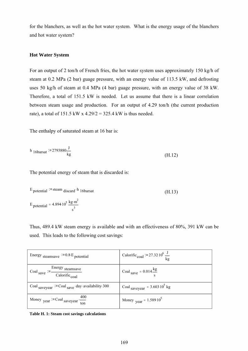
169

for the blanchers, as well as the hot water system. What is the energy usage of the blanchers

and hot water system?

Hot Water System

For an output of 2 ton/h of French fries, the hot water system uses approximately 150 kg/h of

steam at 0.2 MPa (2 bar) guage pressure, with an energy value of 113.5 kW, and defrosting

uses 50 kg/h of steam at 0.4 MPa (4 bar) guage pressure, with an energy value of 38 kW.

Therefore, a total of 151.5 kW is needed. Let us assume that there is a linear correlation

between steam usage and production. For an output of 4.29 ton/h (the current production

rate), a total of 151.5 kW x 4.29/2 = 325.4 kW is thus needed.

The enthalpy of saturated steam at 16 bar is:

h 16barsat 2793880 Jkg (H.12)

The potential energy of steam that is discarded is:

E potential steam discard h 16barsat.

(H.13)

E potential 4.894 105. kg m2.

s3=

Thus, 489.4 kW steam energy is available and with an effectiveness of 80%, 391 kW can be

used. This leads to the following cost savings:

Energy steamsave 0.8 E potential. Calorificcoal 27.32 106. J

kg

Coal saveEnergy steamsave

Calorificcoal Coal save 0.014 kgs

=

Coal saveyear Coal save day. availability. 300. Coal saveyear 3.603 105. kg=

Money year Coal saveyear400ton

. Money year 1.589 105.=

Table H. 1: Steam cost savings calculations

170

If the waste steam that is discarded and 80% of the heat are recaptured and transferred to the

hot water system and blanchers, R158 900 will be saved per annum.

171

I APPENDIX: CALCULATIONS FOR INSTALLATION OF OPTICAL SORTER IN

PRODUCTION LINE

172

I.1 Calculations for Installation of Optical Sorter in Production Line

Installing an optical sorter in the production line will lead to higher sorting effectiveness. At

this stage, 10 workers are employed to manually sort out the defects.

Figure I. 1: Production line with optical sorter inserted

Specifications for the fries are as follows:

2% of packed fries are defective.

Incoming defects through the year:

60% of year 15% defects, able to reach specification.

25% of year 20% defects, unable to reach specification, but can only get to 4% defects.

15% of year < 10% defects, able to reach specification.

Workers at the inspection line:

At inspection line 1, 6 workers are responsible for removing 60% of the defects.

At inspection line 2, 4 workers are responsible for removing 40% of the defects.

Temperature of fries from inspection belt 1:

173

After inspection belt 1:

Blancher 1 20 oC

Blancher 2

Blancher 3 70 oC, then drops to 55 oC

Predryers (atmospheric exposure)

Dryers 1 – 6 40 oC (29.79% to evaporate of incoming product)

Fryer 100 oC (15.86% to evaporate of incoming product)

Defatter

Precooler

Flow freezer -20 oC

Shaker -14 oC

After inspection belt 2:

Packaging -6 oC

Palletising -5 oC

Blast freezer -20 oC

Cooling rooms -20 oC

Table I. 1: Product temperatures on production line

Total percentage of defects taken as an average over a year:

60% per year at (15 - 2)% = 7.8%

25% per year at (20 - 4)% = 4%

15% per year at (5 - 2)% = 0.75%

Thus, the total defects over a year as average, ηline= 12.25 %.

Of this 12.25%, 60% (7.35% defects) is removed at inspection line 1, and 40% is removed at

inspection line 2 (4.90% defects).

Defects Sorted with Optical Sorter

The optical sorter will remove all the defects at inspection line 1, whereas the 0.1% defects at

inspection line 2 (formed by the fryer) will be removed manually, but now only one worker is

needed, or that 0.1% can be left to fit into specifications. This means (12.25 - 0.1)% =

174

12.15% is removed at line 1. This difference in removed defects (12.15 - 7.35)% will cause

an energy saving, as well as a saving of 9 workers’ labour. The energy spent on 1 000 kg/h

fries starting from inspection line are calculated as follow:

Energy Saved in Blancher

Specific heat of potato:

c ppotato 3780 Jkg K. (I.1)

Mass flow of potatoes in:

m pin 1000 kghr (I.2)

Percentage of difference sorted out at inspection line:

η line1 0.1245 0.0753( ) (I.3)

Product temperature difference in blanchers:

Δ T blanchers 70 20( ) K (I.4)

Mass flow of defects saved:

m saved η line1 m pin. (I.5)

m saved 0.014 kgs

=

Blancher energy saved:

E blancher m saved c ppotato. Δ T blanchers. (I.6)

E blancher 2.583 103. W=

175

Energy Saved in Dryer

Product temperature difference Δ T dryers 40 55( ) K

Percentage of mass of fries lost due to

evaporation before dryer

η evap 1 0.020833( )

Mass flow of product into dryer m dryerin η evap m saved.

Latent heat of evaporation of moisture h fgproduct 2260000 Jkg

Percentage of mass lost in dryer η dryer 1 0.2979( )

Energy saved in dryer

E dryer η dryer m dryerin. h fgproduct. E dryer 2.123 104. W=

Table I. 2: Energy savings calculations for dryer

Energy Saved in Fryer

Mass flow into fryer m fryerin η dryer m dryerin.

Product temperature diference Δ T fryer 100 40( ) K

Percentage of mass evaporated η fryer 1 0.1586( )

Energy saved in fryer

E fryer η fryer m fryerin. h fgproduct. m fryerin c ppotato. Δ T fryer. E fryer 2 104. W=

Table I. 3: Energy savings calculations for fryer

Energy Saved in Flow Freezer

Mass flow into freezer m flowfreezer η fryer m fryerin.

Product temperature difference Δ T flowfreezer 40 20( )( ) K

Energy saved in flow freezer

E freezer m flowfreezer c ppotato. Δ T flowfreezer. E freezer 1.793 103. W=

Table I. 4: Energy savings calculations for flow freezer

176

I.1.1 Conclusion

This is only the energy saved when looking at inspection line 1 and ignoring the gains in

terms of shorter exposure of the final product, because fewer workers were needed to sort

defects. The total energy saved for 1 000 kg/h fries just before inspection line 1:

E totalsaved E blancher E dryer E fryer E freezer (I.7)

E totalsaved 4.561 104. W=

The above calculations were done for 1 000 kg/h at inspection line 1. Currently, production is

run at approximately 7 500 kg/hr in. This gives a total of 5482.5 kg/h. Thus, the total energy

that is saved is:

E currentsaved5482.51000

E totalsaved. (I.8)

E currentsaved 2.5 105. W=

Costing in terms of coal:

( )kWE

EEEE

avedtotslcoals

fryerdryerblancheravedtotslcoals

188.2401000

5.5482

=

++⋅⎟⎠⎞

⎜⎝⎛=

(I.9)

Costing in terms of electricity with coefficient of performance, COP = 2.5:

WE

EE

totalelec

freezertotalelec

9.39315.21000

5.5482

=

⋅⎟⎠⎞

⎜⎝⎛=

(I.10)

Currently, the cost for coal is R0.0157/MJ and for electricity R0.0446/MJ. Assuming the

plant is operating 24 hours per day and 340 days per year, the savings per year would be:

Coal cost0.0157

106 J Elec cost

0.0446

106 J

177

tavedtotalcoalscoal CoalshdaysESavings cos360024340 ⋅⋅⋅⋅= 30.110801RSavingscoal =

ttotalelecelec ElecshdaysESavings cos360024340 ⋅⋅⋅⋅=

46.5151RSavingselec =

Table I. 5: Energy savings calculation table

The salary savings due to nine workers replaced by the optical sorter and assuming an hourly

rate of R8 and two 12-hour shifts for 340 days, are as follows:

Salary savings 9 8. 24. 340.

(I.11)

Salary savings 5.875 105.=

Salary savings of R587 500 per annum is possible. Thus, the total savings from the optical

sorter are:

76.703452RSavings

SavingsSavingsSalarySavings

total

eleccoalsavingstotal

=

++= (I.12)

For the optical sorter, one needs to budget 10% of the gross value for maintenance for the first

two years and thereafter 20%.

Cost of Optical Sorter

00.1300000RCosttotal = (I.13)

Maintenance for the first two years at 10% of the gross value:

Cost maintenance 0.1 Cost opticalsorter.

Payback period:

178

( )1003.3

17.01ln

17.076.573452

103.11

1ln 6

=+

⎟⎟⎟⎟

⎠

⎞

⎜⎜⎜⎜

⎝

⎛

⋅⋅

−=

n

n

(I.14)

Thus, in 2.7 years (35 months) the optical sorter will be paid in full.

Savings Realised Through Isolated (Shortened) Sorting Line

By eliminating the sorting line, it is possible to decrease the temperature increase of the final

product by isolating the whole area and ensuring a shorter exposure time of fries to the

environment. Let us say that temperature increase and exposure time are directly proportional

and that by isolating the area around the fries, it is possible to get the environment

temperature down to 0 oC – 5 oC. Therefore, the final mass flow of 3 425 kg/h frozen fries

will experience a decrease in temperature increase from -6 oC to -14 oC. This will result in

savings of:

m finished 3425 kghr

Δ T decrease 6 14( ) K

E finishedproduct c ppotato m finished. Δ T decrease.

E finishedproduct 2.877 104. W=

Savings finishedyear 340 day E finishedproduct. Elec cost. Savings finishedyear 3.769 104.=

Table I. 6: Sorting line savings

From the above calculation, it was estimated that R37 690 can be saved annually on reduced

electricity cost due to reduced heat gain of the frozen product.

179

J APPENDIX: DRYER TEST MEASUREMENTS AND CALCULATIONS

180

J.1 Dryer Test Measurements

Section Dry-bulb Wet-bulb TFries

Outside plant 15.8 13.3

20.7 17.0 Inside plant

21.4 17.0

82.5 35.1 6 bo

74.6 32.1

25.6 23.8 6 onder

25.2 23.6

21.6

37.1 28.8 5 onder

36.5 28.0

39.7 33.8 5 bo

39.1 33.5

32.5

62.6 37.7 4 bo

63.9 37.9

45.0 37.8 4 onder

42.3 38.4

37.2

78.6 47.2 3 onder

79.2 47.4

52.5 43.1 3 bo

52.7 43.1

44.3

74.4 43.8 2 bo

77.6 44.8

53.6 44.0 2 onder

53.6 44.9

44.0

71.7 44.9 1 onder

75.5 45.6

39.5 34.7 1 bo

36.4 31.4

33.7

Table J. 1: Dryer test measurements

181

J.2 Dryer Test Calculations

Outside air Evaporation enthalpy of water

Tdb Tnb Patm ifgwo 21.100 15.100 101325 2501600

Section Tdb [K] Tnb [K] Pz1 [Pa] Pz2 [Pa] Outside 21.1 294.25 15.1 288.25 2501.057 1715.1431.000 35.0 308.15 28.4 301.55 5623.136 3868.1641.500 62.7 335.85 39.2 312.35 22551.243 7068.2422.000 67.7 340.85 38.4 311.55 28195.073 6770.5822.500 46.8 319.95 37.4 310.55 10508.034 6413.7923.000 48.9 322.05 36.4 309.55 11680.814 6073.3833.500 62.0 335.15 35.1 308.25 21843.660 5654.3084.000 45.3 318.45 30.2 303.35 9733.632 4291.5444.500 36.3 309.45 30.6 303.75 6040.219 4390.9175.000 34.5 307.65 28.9 302.05 5469.497 3981.9555.500 32.6 305.75 24.2 297.35 4918.357 3018.8066.000 86.6 359.75 34.9 308.05 61531.893 5592.1126.500 31.4 304.55 25.0 298.15 4595.677 3166.717

ωz2 cpa1 cpa2 cpv1 cpv2 ha1 ha2 0.011 1006.762 1006.597 1880.646 1875.421 21242.68 15199.610.025 1007.275 1007.009 1893.962 1887.368 35254.64 28599.070.047 1008.822 1007.465 1931.543 1898.498 63253.11 39492.640.045 1009.173 1007.428 1940.923 1897.611 68321.01 38685.23

0.042 1007.850 1007.382 1907.573 1896.517 47167.38 37676.090.040 1007.966 1007.337 1910.313 1895.441 49289.51 36667.060.037 1008.774 1007.280 1930.310 1894.066 62544.00 35355.520.028 1007.770 1007.078 1905.682 1889.110 45651.98 30413.750.028 1007.332 1007.094 1895.334 1889.502 36566.17 30817.060.025 1007.254 1007.028 1893.441 1887.848 34750.26 29103.110.019 1007.174 1006.861 1891.495 1883.441 32833.87 24366.040.036 1010.694 1007.271 1987.537 1893.857 87526.14 35153.760.020 1007.125 1006.888 1890.293 1884.176 31623.73 25172.20

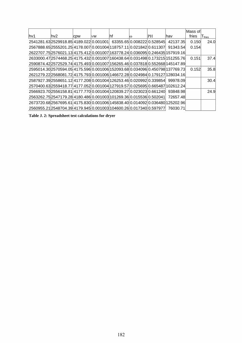
182

hv1 hv2 cpw νw hf ω ΡΗ hav Mass of

fries Tfries 2541281.63 2529918.85 4189.022 0.001001 63355.65 0.008222 0.528545 42137.35 0.150 24.02567888.65 2555201.25 4178.007 0.001004 118757.11 0.021842 0.611307 91343.54 0.154 2622707.75 2576021.13 4175.412 0.001007 163778.24 0.036095 0.246435 157919.16 2633000.47 2574468.25 4175.432 0.001007 160438.64 0.031498 0.173215 151255.76 0.151 37.42590874.42 2572529.74 4175.493 0.001007 156265.46 0.037818 0.552668 145147.89 2595014.30 2570594.05 4175.596 0.001006 152093.68 0.034096 0.450798 137769.73 0.152 35.82621279.22 2568081.72 4175.793 0.001006 146672.28 0.024984 0.179127 128034.16 2587927.39 2558651.12 4177.208 0.001004 126253.46 0.020992 0.339854 99978.09 30.42570400.63 2559418.77 4177.052 0.001004 127919.57 0.025695 0.665487 102612.24 2566923.70 2556158.81 4177.770 0.001004 120839.27 0.023023 0.661240 93848.98 24.92563262.75 2547179.28 4180.486 0.001003 101269.36 0.015536 0.502041 72657.48 2673720.68 2567695.61 4175.830 0.001006 145838.40 0.014092 0.036480 125202.96 2560955.21 2548704.39 4179.945 0.001003 104600.26 0.017340 0.597977 76030.71

Table J. 2: Spreadsheet test calculations for dryer

183

K APPENDIX: VISUAL BASIC PROGRAM FOR HEAT EXCHANGER ANALYSIS

184

K.1 Heat Exchanger Code

Option Explicit Dim i As Integer Dim j As Integer Dim m As Integer Dim pi Dim Nn 'Segment flow conditions: Dim dio As Double Dim mw As Double, kss Dim txtri As Double Dim txtAe As Double Dim txtAp As Double Dim txtmse As Double Dim txtmwe As Double Dim tw As Double Dim dx As Double Dim eqBend As Double 'Subprocedure for calculations Dim Tsin(0 To 100, 0 To 100), Twin(0 To 100, 0 To 100), Hsin(0 To 100, 0 To 100), Hwin(0 To 100, 0 To 100) Dim rhos(0 To 100, 0 To 100), kviscs(0 To 100, 0 To 100), ks(0 To 100, 0 To 100), Prs(0 To 100, 0 To 100) Dim Res(0 To 100, 0 To 100), Nuds(0 To 100, 0 To 100), hcs(0 To 100, 0 To 100), rhow(0 To 100, 0 To 100) Dim kviscw(0 To 100, 0 To 100), dviscs(0 To 100, 0 To 100), kw(0 To 100, 0 To 100), Prw(0 To 100, 0 To 100), Rew(0 To 100, 0 To 100) Dim f(0 To 100, 0 To 100), Nudw(0 To 100, 0 To 100), hcw(0 To 100, 0 To 100), term1(0 To 100, 0 To 100) Dim term3(0 To 100, 0 To 100), UP(0 To 100, 0 To 100), deltaQ(0 To 100, 0 To 100), Hsout(0 To 100, 0 To 100) Dim Hwout(0 To 100, 0 To 100), Tsout(0 To 100, 0 To 100), Twout(0 To 100, 0 To 100), deltaPs(0 To 100, 0 To 100) Dim Twt(0 To 100, 0 To 100), fdrag(0 To 100, 0 To 100), deltaPw(0 To 100, 0 To 100), Rys(0 To 100, 0 To 100), Kloss(0 To 100, 0 To 100) Dim term2, msCond(0 To 100, 0 To 100), msCondTotal(0 To 100, 0 To 100), mse(0 To 100, 0 To 100), mseOut(0 To 100, 0 To 100) Dim bFin(0 To 100, 0 To 100), zFin(0 To 100, 0 To 100), min2epowerzFin(0 To 100, 0 To 100), tanhzFin(0 To 100, 0 To 100) Dim velFree(0 To 100, 0 To 100), velMax(0 To 100, 0 To 100), deltaPwBend(0 To 100, 0 To 100), deltaPwPrevious Dim Atotal Dim Nrow As Integer, numRow, numCol, numPipe, numFin Dim ibegin As Integer Dim iend As Integer

185

Dim iStart As Integer Dim iFinish As Integer Dim deltaPsTotal(0 To 100, 0 To 100) Dim deltaPwTotal(0 To 100, 0 To 100) Dim deltaQTotal(0 To 100, 0 To 100) Dim deltaAtotal, deltaAtotalPrevious Dim mseTotalExit Dim betaFin(0 To 100, 0 To 100) Dim thetaFin(0 To 100, 0 To 100) Dim term3Fin(0 To 100, 0 To 100) Dim thetaFintotal(0 To 100, 0 To 100) Dim UFins(0 To 100, 0 To 100) Private Sub cmdcalculate_Click() 'Segment flow conditions: pi = 3.141592654 dio = Val(txtdo.Text) mw = Val(txtmw.Text) numCol = Val(txtNrc.Text) numRow = Val(txtNrows.Text) numPipe = Val(txtnumPipes.Text) widthHE = Val(txtWidth.Text) kss = Val(txtkss.Text) RelRough = Val(txtRelRough.Text) dx = Val(txtls.Text) numFin = 0 tw = Val(txttw.Text) At = widthHE * widthHE eqBend = 1.2 txtri = dio / 2 - tw numElem = numCol * numPipe txtAe = At / numElem txtAp = pi * txtri ^ 2 txtmse = txtms / numElem txtmwe = mw / numPipe ibegin = 0 iend = widthHE / dx - 1 Twin(0, 0) = Val(txtTwin.Text) For i = ibegin To iend Tsin(i, 0) = Val(txtTsin.Text) mse(i, 0) = txtmse Next i m = numRow

186

iStart = ibegin iFinish = iend parameterj = -1 deltaPsPrevious = 0 deltaPwPrevious = 0 deltaQPrevious = 0 deltaAtotalPrevious = 0 msCondPrevious = 0 For j = 0 To m parameterj = -parameterj For i = ibegin To iend Step parameterj Nrow = 0 Call CalculationFins(i, j, Twin(), Tsin(), Twout(), Tsout(), deltaQ(), deltaPs(), deltaPw(), deltaPwBend(), Atotal) If parameterj = 1 Then Twin(i + 1, j) = Twout(i, j) Else If i - 1 >= iend Then Twin(i - 1, j) = Twout(i, j) End If Tsin(i, j + 1) = Tsout(i, j) mse(i, j + 1) = mseOut(i, j) 'Pressurefall limit for water in heat exchanger deltaPwTotal(i, j) = deltaPw(i, j) + deltaPwPrevious deltaPwPrevious = deltaPwTotal(i, j) msCondTotal(i, j) = msCond(i, j) + msCondPrevious msCondPrevious = msCondTotal(i, j) 'Heat transfer summation deltaQTotal(i, j) = deltaQ(i, j) + deltaQPrevious deltaQPrevious = deltaQTotal(i, j) deltaAtotal = deltaAtotalPrevious + Atotal deltaAtotalPrevious = deltaAtotal Next i If parameterj = -1 Then deltaPwPrevious = deltaPwTotal(iStart, j) + deltaPwBend(iStart, j) Else deltaPwPrevious = deltaPwTotal(iFinish, j) + deltaPwBend(iFinish, j) End If Twin(iend, j + 1) = Twout(iend, j) ibeginnew = ibegin ibegin = iend iend = ibeginnew 'Pressurefall limit for steam in heat exchanger deltaPsTotal(iStart, j) = deltaPs(iStart, j) + deltaPsPrevious deltaPsPrevious = deltaPsTotal(iStart, j)

187

Next j For j = 0 To m For i = 0 To iFinish ListTwin.AddItem Format(Twin(i, j), "0.000000") ListTsout.AddItem Format(Tsin(i, j), "0.000000") ListdeltaQ.AddItem Format(deltaQ(i, j), "0.000000") ListdeltaPs.AddItem Format(deltaPs(i, j), "0.000000") ListdeltaPw.AddItem Format(deltaPw(i, j), "0.000000") Next i Next j msePrevious = 0 For i = 0 To iFinish mseTotalExit = mse(i, m) + msePrevious msePrevious = mseTotalExit Next i End Sub Private Sub CmdCalculationFins_Click() 'Segment flow conditions: pi = 3.141592654 dio = Val(txtdo.Text) mw = Val(txtmw.Text) numCol = Val(txtNrc.Text) numRow = Val(txtNrows.Text) numPipe = Val(txtnumPipes.Text) widthHE = Val(txtWidth.Text) kss = Val(txtkss.Text) RelRough = Val(txtRelRough.Text) dx = Val(txtls.Text) numFin = Val(txtnumFins.Text) tw = Val(txttw.Text) At = widthHE * widthHE eqBend = 1.2 txtri = dio / 2 - tw numElem = numCol * numPipe txtAe = At / numElem txtAp = pi * txtri ^ 2 txtmse = txtms / numElem txtmwe = mw / numPipe ibegin = 0

188

iend = widthHE / dx - 1 Twin(0, 0) = Val(txtTwin.Text) For i = ibegin To iend Tsin(i, 0) = Val(txtTsin.Text) mse(i, 0) = txtmse Next i m = numRow iStart = ibegin iFinish = iend parameterj = -1 deltaPsPrevious = 0 deltaPwPrevious = 0 deltaQPrevious = 0 deltaAtotalPrevious = 0 msCondPrevious = 0 For j = 0 To m parameterj = -parameterj For i = ibegin To iend Step parameterj Nrow = 0 Call CalculationFins(i, j, Twin(), Tsin(), Twout(), Tsout(), deltaQ(), deltaPs(), deltaPw(), deltaPwBend(), Atotal) If parameterj = 1 Then Twin(i + 1, j) = Twout(i, j) Else If i - 1 >= iend Then Twin(i - 1, j) = Twout(i, j) End If Tsin(i, j + 1) = Tsout(i, j) mse(i, j + 1) = mseOut(i, j) 'Pressurefall limit for water in heat exchanger deltaPwTotal(i, j) = deltaPw(i, j) + deltaPwPrevious deltaPwPrevious = deltaPwTotal(i, j) msCondTotal(i, j) = msCond(i, j) + msCondPrevious msCondPrevious = msCondTotal(i, j) 'Heat transfer summation deltaQTotal(i, j) = deltaQ(i, j) + deltaQPrevious deltaQPrevious = deltaQTotal(i, j) deltaAtotal = deltaAtotalPrevious + Atotal deltaAtotalPrevious = deltaAtotal Next i If parameterj = -1 Then deltaPwPrevious = deltaPwTotal(iStart, j) + deltaPwBend(iStart, j) Else deltaPwPrevious = deltaPwTotal(iFinish, j) + deltaPwBend(iFinish, j)

189

End If Twin(iend, j + 1) = Twout(iend, j) ibeginnew = ibegin ibegin = iend iend = ibeginnew 'Pressurefall limit for steam in heat exchanger deltaPsTotal(iStart, j) = deltaPs(iStart, j) + deltaPsPrevious deltaPsPrevious = deltaPsTotal(iStart, j) Next j For j = 0 To m For i = 0 To iFinish ListTwin.AddItem Format(Twin(i, j), "0.000000") ListTsout.AddItem Format(Tsin(i, j), "0.000000") ListdeltaQ.AddItem Format(deltaQ(i, j), "0.000000") ListdeltaPs.AddItem Format(deltaPs(i, j), "0.000000") ListdeltaPw.AddItem Format(deltaPw(i, j), "0.000000") Next i Next j msePrevious = 0 For i = 0 To iFinish mseTotalExit = mse(i, m) + msePrevious msePrevious = mseTotalExit Next i End Sub Private Sub cmdCombi_Click() 'Segment flow conditions: pi = 3.141592654 dio = Val(txtdo.Text) mw = Val(txtmw.Text) numCol = Val(txtNrc.Text) numRow = Val(txtNrows.Text) numPipe = Val(txtnumPipes.Text) widthHE = Val(txtWidth.Text) kss = Val(txtkss.Text) RelRough = Val(txtRelRough.Text) dx = Val(txtls.Text) numFin = Val(txtnumFins.Text) tw = Val(txttw.Text) At = widthHE * widthHE

190

eqBend = 1.2 txtri = dio / 2 - tw numElem = numCol * numPipe txtAe = At / numElem txtAp = pi * txtri ^ 2 txtmse = txtms / numElem txtmwe = mw / numPipe ibegin = 0 iend = widthHE / dx - 1 Twin(0, 0) = Val(txtTwin.Text) For i = ibegin To iend Tsin(i, 0) = Val(txtTsin.Text) mse(i, 0) = txtmse Next i m = numRow iStart = ibegin iFinish = iend parameterj = -1 deltaPsPrevious = 0 deltaPwPrevious = 0 deltaQPrevious = 0 deltaAtotalPrevious = 0 msCondPrevious = 0 For j = 0 To 9 parameterj = -parameterj For i = ibegin To iend Step parameterj Nrow = 0 Call CalculationFins(i, j, Twin(), Tsin(), Twout(), Tsout(), deltaQ(), deltaPs(), deltaPw(), deltaPwBend(), Atotal) If parameterj = 1 Then Twin(i + 1, j) = Twout(i, j) Else If i - 1 >= iend Then Twin(i - 1, j) = Twout(i, j) End If Tsin(i, j + 1) = Tsout(i, j) mse(i, j + 1) = mseOut(i, j) 'Pressurefall limit for water in heat exchanger deltaPwTotal(i, j) = deltaPw(i, j) + deltaPwPrevious deltaPwPrevious = deltaPwTotal(i, j) msCondTotal(i, j) = msCond(i, j) + msCondPrevious msCondPrevious = msCondTotal(i, j)

191

'Heat transfer summation and heat transfer area summation deltaQTotal(i, j) = deltaQ(i, j) + deltaQPrevious deltaQPrevious = deltaQTotal(i, j) deltaAtotal = deltaAtotalPrevious + Atotal deltaAtotalPrevious = deltaAtotal Next i If parameterj = -1 Then deltaPwPrevious = deltaPwTotal(iStart, j) + deltaPwBend(iStart, j) Else deltaPwPrevious = deltaPwTotal(iFinish, j) + deltaPwBend(iFinish, j) End If Twin(iend, j + 1) = Twout(iend, j) ibeginnew = ibegin ibegin = iend iend = ibeginnew 'Pressurefall limit for steam in heat exchanger deltaPsTotal(iStart, j) = deltaPs(iStart, j) + deltaPsPrevious deltaPsPrevious = deltaPsTotal(iStart, j) Next j ibegin = iStart iend = iFinish parameterj = -1 For j = 10 To m numFin = 0 parameterj = -parameterj For i = ibegin To iend Step parameterj Call CalculationFins(i, j, Twin(), Tsin(), Twout(), Tsout(), deltaQ(), deltaPs(), deltaPw(), deltaPwBend(), Atotal) If parameterj = 1 Then Twin(i + 1, j) = Twout(i, j) Else If i - 1 >= iend Then Twin(i - 1, j) = Twout(i, j) End If Tsin(i, j + 1) = Tsout(i, j) mse(i, j + 1) = mseOut(i, j) 'Pressurefall limit for water in heat exchanger deltaPwTotal(i, j) = deltaPw(i, j) + deltaPwPrevious deltaPwPrevious = deltaPwTotal(i, j) msCondTotal(i, j) = msCond(i, j) + msCondPrevious msCondPrevious = msCondTotal(i, j) 'Heat transfer summation deltaQTotal(i, j) = deltaQ(i, j) + deltaQPrevious deltaQPrevious = deltaQTotal(i, j) deltaAtotal = deltaAtotalPrevious + Atotal

192

deltaAtotalPrevious = deltaAtotal Next i If parameterj = -1 Then deltaPwPrevious = deltaPwTotal(iStart, j) + deltaPwBend(iStart, j) Else deltaPwPrevious = deltaPwTotal(iFinish, j) + deltaPwBend(iFinish, j) End If Twin(iend, j + 1) = Twout(iend, j) ibeginnew = ibegin ibegin = iend iend = ibeginnew 'Pressurefall limit for steam in heat exchanger deltaPsTotal(iStart, j) = deltaPs(iStart, j) + deltaPsPrevious deltaPsPrevious = deltaPsTotal(iStart, j) Next j For j = 0 To m For i = 0 To iFinish ListTwin.AddItem Format(Twin(i, j), "0.000000") ListTsout.AddItem Format(Tsin(i, j), "0.000000") ListdeltaQ.AddItem Format(deltaQ(i, j), "0.000000") ListdeltaPs.AddItem Format(deltaPs(i, j), "0.000000") ListdeltaPw.AddItem Format(deltaPw(i, j), "0.000000") Next i Next j msePrevious = 0 For i = 0 To iFinish mseTotalExit = mse(i, m) + msePrevious msePrevious = mseTotalExit Next i End Sub Private Sub cmddisplay_Click() picPlot.Print deltaPsTotal(iStart, m), "Total steam pressure fall" picPlot.Print deltaPwTotal(iend, m), "Total water pressure fall" picPlot.Print deltaQTotal(iFinish, m), "Total heat transfer" picPlot.Print deltaAtotal, "Total heat transfer surface (m2)" picPlot.Print msCondTotal(iFinish, m), "Total condensate per column" picPlot.Print mseTotalExit, "Total steam flow at exit" picPlot.Print (mseTotalExit + msCondTotal(iFinish, m)) * 14, "total water out" End Sub

193

Private Sub cmdok_Click() End End Sub Private Sub CalculationFins(i, j, Twin(), Tsin(), Twout(), Tsout(), deltaQ(), deltaPs(), deltaPw(), deltaPwBend(), Atotal) 'Calculation of Overall heat transfer coefficient, UA 'Calculation of convective heat transfer coefficient for the steam side: Hsin(i, j) = mse(i, j) * (1986.3 * Tsin(i, j) + 1935600) + msCond(i, j) * hfs '(Correlation obtain from Schmidt, 1969) Hwin(i, j) = txtmwe * (4185.1 * Twin(i, j) - 1143000) '(Correlation obtain from Schmidt, 1969) '__________________________________________________________________________________________________________ 'Steam properties at txtTsin: rhos(i, j) = 3.4503922053E-06 * Tsin(i, j) ^ 2 - 0.00420531051 * Tsin(i, j) + 1.6780736016 kviscs(i, j) = 0.000000146042 * Tsin(i, j) - 0.00003422741 ks(i, j) = 0.0000837273 * Tsin(i, j) - 0.0066655591 Prs(i, j) = -0.0002418182 * Tsin(i, j) + 1.073053 Res(i, j) = (mse(i, j) * dio) / (rhos(i, j) * txtAe * kviscs(i, j)) If Res(i, j) < 10000 Then Nuds(i, j) = 0.3 + (0.62 * (Res(i, j) ^ 0.5) * Prs(i, j) ^ (1 / 3)) / ((1 + (0.4 / Prs(i, j)) ^ (2 / 3)) ^ (1 / 4)) ElseIf 10000 <= Res(i, j) < 400000 Then Nuds(i, j) = 0.3 + (((0.62 * (Res(i, j) ^ 0.5) * Prs(i, j) ^ (1 / 3)) / (1 + (0.4 / Prs(i, j)) ^ (2 / 3)) ^ (1 / 4))) * (1 + (Res(i, j) / 282000) ^ 0.5) ElseIf Res(i, j) > 400000 Then Nuds(i, j) = 0.3 + (((0.62 * (Res(i, j) ^ 0.5) * Prs(i, j) ^ (1 / 3)) / (1 + (0.4 / Prs(i, j)) ^ (2 / 3)) ^ (1 / 4))) * ((1 + (Res(i, j) / 282000) ^ (5 / 8)) ^ 0.8) End If 'Convection heat transfer coefficient for steam rhol = 957.8544 rhov = 0.59776 g = 9.81 ksl = 0.681 mul = 279 * 10 ^ (-6) hfs = 419040 hgs = 2676100 hfgs = 2257000 If Tsin(i, j) > 373.15 Then hcs(i, j) = ks(i, j) * Nuds(i, j) / dio Else Nrow = Nrow + 1 hcs(i, j) = 0.728 * (((rhol - rhov) * g * hfgs * (ksl) ^ 3) / (Nrow * (mul / rhol) * dio * (Tsin(i, j) - Twin(i, j)))) ^ 0.25 End If

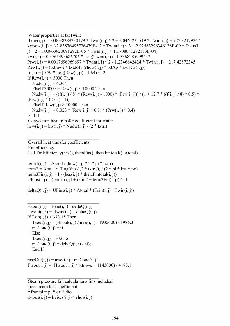
194

'__________________________________________________________________________________________________________ 'Water properties at txtTwin: rhow(i, j) = -0.0038388230179 * Twin(i, j) ^ 2 + 2.0464231519 * Twin(i, j) + 727.82179247 kviscw(i, j) = (-2.83876495726479E-12 * Twin(i, j) ^ 3 + 2.92563296346138E-09 * Twin(i, j) ^ 2 - 1.00963920098292E-06 * Twin(i, j) + 1.1708641282173E-04) kw(i, j) = 0.3765493686706 * Log(Twin(i, j)) - 1.5368285999447 Prw(i, j) = 0.0017696969697 * Twin(i, j) ^ 2 - 1.2346642424 * Twin(i, j) + 217.42872345 Rew(i, j) = (txtmwe * txtdo) / (rhow(i, j) * txtAp * kviscw(i, j)) f(i, j) = (0.79 * Log(Rew(i, j)) - 1.64) ^ -2 If Rew(i, j) < 3000 Then Nudw(i, j) = 4.364 ElseIf 3000 <= Rew(i, j) < 10000 Then Nudw(i, j) = ((f(i, j) / 8) * (Rew(i, j) - 1000) * (Prw(i, j))) / (1 + 12.7 * ((f(i, j) / 8) ^ 0.5) * (Prw(i, j) ^ (2 / 3) - 1)) ElseIf Rew(i, j) > 10000 Then Nudw(i, j) = 0.023 * (Rew(i, j) ^ 0.8) * (Prw(i, j) ^ 0.4) End If 'Convection heat transfer coefficient for water hcw(i, j) = kw(i, j) * Nudw(i, j) / (2 * txtri) '__________________________________________________________________________________________________________ 'Overall heat transfer coefficients: 'Fin efficiency Call FinEfficiency(hcs(), thetaFin(), thetaFintotal(), Atotal) term1(i, j) = Atotal / (hcw(i, j) * 2 * pi * txtri) term2 = Atotal * (Log(dio / (2 * txtri))) / (2 * pi * kss * tw) term3Fin(i, j) = 1 / (hcs(i, j) * thetaFintotal(i, j)) UFins(i, j) = (term1(i, j) + term2 + term3Fin(i, j)) ^ -1 deltaQ(i, j) = UFins(i, j) * Atotal * (Tsin(i, j) - Twin(i, j)) '__________________________________________________________________________________________________________ Hsout(i, j) = Hsin(i, j) - deltaQ(i, j) Hwout(i, j) = Hwin(i, j) + deltaQ(i, j) If Tsin(i, j) > 373.15 Then Tsout(i, j) = (Hsout(i, j) / mse(i, j) - 1935600) / 1986.3 msCond(i, j) = 0 Else Tsout(i, j) = 373.15 msCond(i, j) = deltaQ(i, j) / hfgs End If mseOut(i, j) = mse(i, j) - msCond(i, j) Twout(i, j) = (Hwout(i, j) / txtmwe + 1143000) / 4185.1 '__________________________________________________________________________________________________________ 'Steam pressure fall calculations fins included 'freestream loss coefficient Afrontal = pi * dx * dio dviscs(i, j) = kviscs(i, j) * rhos(i, j)

195

velFree(i, j) = mse(i, j) / (rhos(i, j) * Afrontal) st = 0.05 velMax(i, j) = velFree(i, j) * (st / (st - dio)) deltaPs(i, j) = (j + 1) * rhos(i, j) * velMax(i, j) ^ 2 * 0.5 'Water pressure drop calculations Twt(i, j) = deltaQ(i, j) / hcw(i, j) * txtAp ^ 2 + Twin(i, j) fdrag(i, j) = 0.3086 * ((Log(6.9 / Rew(i, j))) / Log(10) + (RelRough / 3.75) ^ 1.11) ^ (-2) deltaPw(i, j) = fdrag(i, j) * dx ^ 2 * mw ^ 2 / (2 * txtri * rhow(i, j) * txtAp ^ 2) deltaPwBend(i, j) = fdrag(i, j) * eqBend ^ 2 * mw ^ 2 / (2 * txtri * rhow(i, j) * txtAp ^ 2) End Sub Private Function FinEfficiency(hcs(), thetaFin(), thetaFintotal(), Atotal) 'Fin properties tFin = Val(txtfinThick.Text) kFin = kss bFin(i, j) = (hcs(i, j) / (0.5 * tFin * kFin)) ^ 0.5 r2Fin = Val(txtfindia.Text) / 2 r1Fin = dio / 2 phiFin = (r2Fin / r1Fin - 1) * (1 + 0.35 * Log(r2Fin / r1Fin)) zFin(i, j) = bFin(i, j) * dio * phiFin / 2 SFin = 2 * pi * (r2Fin ^ 2 - r1Fin ^ 2) AFin = 2 * SFin Atotal = dx * pi * dio + AFin * numFin VFin = 0.5 * SFin * tFin 'Calculation of hyperbolic Tan: min2epowerzFin(i, j) = 1 + (-2 * zFin(i, j)) + (-2 * zFin(i, j)) ^ 2 / 2 + (-2 * zFin(i, j)) ^ 3 / 6 + (-2 * zFin(i, j)) ^ 4 / 24 + (-2 * zFin(i, j)) ^ 5 / 120 tanhzFin(i, j) = (1 - min2epowerzFin(i, j)) / (1 + min2epowerzFin(i, j)) thetaFin(i, j) = tanhzFin(i, j) / zFin(i, j) If numFin >= 1 Then thetaFintotal(i, j) = 1 - AFin * (1 - thetaFin(i, j)) / Atotal Else thetaFintotal(i, j) = 1 End If End Function Private Sub cmdPlot_Click() Dim bo As Double Dim regs As Double Dim onder As Double Dim links As Double Dim yMaks As Double Dim xMaks As Double Dim yDelta As Double Dim xDelta As Double

196

Dim yMin As Double Dim xMin As Double Dim X As Double Dim Y As Double yMaks = -273 yMin = 99999 For X = 1 To ListTwin.ListCount - 1 If yMaks < ListTwin.List(X) Then yMaks = ListTwin.List(X) If yMin > ListTwin.List(X) Then yMin = ListTwin.List(X) Next X xMaks = ListTwin.ListCount xMin = 0 yDelta = yMaks - yMin xDelta = xMaks - xMin ' Kry maksimum y waarde bo = yMaks + 0.05 * yDelta ' Kry minimum y waarde onder = yMin - 0.05 * yDelta ' Kry maksimum x waarde regs = xMaks + 0.05 * xDelta ' Kry minimum x waarde links = xMin - 0.05 * xDelta ' Create plotting window picPlot.Scale (links, bo)-(regs, onder) picPlot.PSet (xMin, yMin) picPlot.Print "Plot of water temperature" picPlot.Line (xMin, yMin)-(xMin, yMaks) picPlot.Line (xMin, yMin)-(xMaks, yMin) picPlot.FillColor = vbBlue picPlot.FillStyle = vbFSSolid For X = 1 To ListTwin.ListCount - 1 ' picPlot.Line (x, ListTwin.List(x))-(x + 1, ListTwin.List(x + 1)) 'picPlot.PSet (x, ListTwin.List(x)), vbRed picPlot.Circle (X, ListTwin.List(X)), 0.08, vbBlue 'picPlot.Circle (X, ListTsout.List(X)), 0.08, vbBlue Next X End Sub Private Sub cmdSave_Click() Open App.Path & "\pressurefallwater.txt" For Output As #1

197

parameterj = -1 ibegin = 0 iend = iFinish For j = 0 To m parameterj = -parameterj For i = ibegin To iend Step parameterj Write #1, i, j, deltaPwTotal(i, j), deltaPsTotal(i, j), deltaQTotal(i, j), hcs(i, j), hcw(i, j), Tsin(i, j), Twin(i, j) Next i ibeginnew = ibegin ibegin = iend iend = ibeginnew Next j Close #1 Open App.Path & "\temperaturewater.txt" For Output As #2 Dim k As Integer For k = 0 To ListTwin.ListCount - 1 Write #2, k, ListTwin.List(k), ListTsout.List(k) Next k Close #2 Open App.Path & "\temperaturesteam.txt" For Output As #3 For j = 0 To m - 1 Write #3, j, Tsin(iStart, j) Next j Close #3 Open App.Path & "\pressurefallsteam.txt" For Output As #4 For j = 0 To m - 1 Write #4, j, deltaPsTotal(iStart, j) Next j Close #4 End Sub Private Sub picPlot_Click() picPlot.Cls End Sub

198

K.2 Heat Exchanger Program Form

Figure K. 1: Heat exchanger program form

199

K.3 Correlations for Steam and Water Properties

Density (kg/m3), specific heat (kJ/kgK), dynamic viscosity (m2/s), thermal conductivity

coefficient (W/mK) and the Prandtl number of steam at atmospheric conditions as functions

of temperature (K):

161.67807360 + T10004.20531051 - T10533.45039220 s-32

s-6 ⋅⋅⋅⋅=sρ

(K. 1)

433.34636668 + T10565.97018907 - T10206.51260504 s-32

s-6 ⋅⋅⋅⋅=psc

(K. 2)

-5

S-7 10433.42274082 - T10821.46041981 ⋅⋅⋅=sμ (K. 3)

910.00666555 - T730.00008372 s⋅=sk (K. 4)

641.07305263 + T10182-2.4181818Pr s-4 ⋅⋅=s (K. 5)

Density (kg/m3), specific heat (kJ/kgK), dynamic viscosity (m2/s), thermal conductivity

coefficient (W/mK) and the Prandtl number of water at atmospheric conditions as functions of

temperature (K):

47727.821792 + T192.04642315 + T10793.83882301- w2w

-3 ⋅⋅⋅=wρ

(K. 6)

004.41366800 + T000-0.0007200 w⋅=pwc (K. 7)

8410.11651081 + T10591.00392900 -

T10022.90713817 + T10193-2.8193473

w3-

2w

-63w

-9

⋅⋅

⋅⋅⋅⋅=wμ (K. 8)

200

994471.53682859 - )86706Ln(T0.37654936 w=wk (K. 9)

45217.428723 + T241.23466424 - T10971.76969696Pr w23 ⋅⋅⋅= −

w

(K. 10)

THERMO ECONOMIC ANALYSIS OF A FRENCH FRIES PROCESSING

Documents

Transcript of THERMO ECONOMIC ANALYSIS OF A FRENCH FRIES PROCESSING