Thermal Physics of Bose & Fermi Gases

Based on lectures given by J.Forshaw at the University of Manchester Sept-Dec ’07Please e-mail me with any comments/corrections: jap@watering.co.uk

J.Pearson

January 2, 2008

Contents

1 Einsteins Model of a Solid 1

2 The Gibbs Factor 4

2.0.1 Example: CO Poisoning . . . . . . . . . . . . . . . . . . . . . . . . . . . . . . 7

2.1 My Grand Partition Function . . . . . . . . . . . . . . . . . . . . . . . . . . . . . . . 7

3 Identical Particles 8

3.1 Distinguishable Particles . . . . . . . . . . . . . . . . . . . . . . . . . . . . . . . . . . 8

3.2 Indistinguishable Particles . . . . . . . . . . . . . . . . . . . . . . . . . . . . . . . . . 8

3.3 Pauli Principle . . . . . . . . . . . . . . . . . . . . . . . . . . . . . . . . . . . . . . . 8

4 The Bose-Einstein & Fermi-Dirac Distributions 9

4.1 Fermi-Dirac Distribution . . . . . . . . . . . . . . . . . . . . . . . . . . . . . . . . . . 10

4.2 Bose-Einstein Distribution . . . . . . . . . . . . . . . . . . . . . . . . . . . . . . . . . 10

4.3 Spin Multiplicity . . . . . . . . . . . . . . . . . . . . . . . . . . . . . . . . . . . . . . 11

5 Classical Limit 11

5.1 Chemical Potential µ . . . . . . . . . . . . . . . . . . . . . . . . . . . . . . . . . . . . 12

5.1.1 Internal Energy & Heat Capacity . . . . . . . . . . . . . . . . . . . . . . . . . 15

5.2 Entropy of an Ideal Gas . . . . . . . . . . . . . . . . . . . . . . . . . . . . . . . . . . 15

6 Fermi Gases 19

i

6.1 Ideal Fermi Gas at T ≈ 0 . . . . . . . . . . . . . . . . . . . . . . . . . . . . . . . . . 20

6.2 Density of States . . . . . . . . . . . . . . . . . . . . . . . . . . . . . . . . . . . . . . 22

6.2.1 3D Density of States . . . . . . . . . . . . . . . . . . . . . . . . . . . . . . . . 23

6.2.2 Low T Corrections to N,U . . . . . . . . . . . . . . . . . . . . . . . . . . . . 29

6.3 Example: Electrons in Metals . . . . . . . . . . . . . . . . . . . . . . . . . . . . . . . 32

6.4 Example: Liquid 3He . . . . . . . . . . . . . . . . . . . . . . . . . . . . . . . . . . . . 33

6.5 Example: Electrons in Stars . . . . . . . . . . . . . . . . . . . . . . . . . . . . . . . . 34

6.5.1 White Dwarf Stars . . . . . . . . . . . . . . . . . . . . . . . . . . . . . . . . . 34

7 Bose Gases 38

7.1 Black Body Radiation . . . . . . . . . . . . . . . . . . . . . . . . . . . . . . . . . . . 41

7.2 Spectral Energy Density . . . . . . . . . . . . . . . . . . . . . . . . . . . . . . . . . . 43

7.2.1 Pressure of a Photon Gas . . . . . . . . . . . . . . . . . . . . . . . . . . . . . 45

8 Lattice Vibrations of a Solid 47

A Colloquial Summary I

B Calculating the Density of States IV

B.1 Energy Space: Non-Relativistic . . . . . . . . . . . . . . . . . . . . . . . . . . . . . . IV

B.2 Energy Space: Ultra-Relativistic . . . . . . . . . . . . . . . . . . . . . . . . . . . . . V

C Deriving FD & BE Distributions VI

ii

1 Einsteins Model of a Solid

Assume: each atom in a solid vibrates independantly about an equilibrium position. The vibrationsare assumed to be simple harmonic, and all of the same frequency.

In a 3D solid, each atom can oscillate in 3 independant directions.i.e. if N oscillators, then N

3 atoms.

Our system is a collection of N independant oscillators. Each oscillator has energy:(ni +

12

)hω (1.1)

Where ni is the quantum number of the ith oscillator: ni = 0, 1, 2, . . .ω = angular frequency of oscillator - remember they all have the same frequency.

Now, we proceed by measuring all energies relative to the ground state (ni = 0). Hence:

εi = nihω (1.2)

Where εi is the energy of the ith oscillator.Now, we have N such oscillators; so the total energy is:

U = (n1 + n2 + n3 + . . .+ nN )hω (1.3)= nhω (1.4)

Hence, n represents the energy of the system, in units of hω.The quantum state of the solid as a whole is specified by the list (n1, n2, n3, . . . , nN ).Clearly, there are several quantum states corresponding to the same total energy. So, how maystates can we have with a system of a particular energy?

Let g(n,N) be the number of possible quantum states when the total energy is nhω.We can easily see/show that:

g(n,N) =(N + n− 1)!n!(N − 1)!

(1.5)

The proof of which is trivial combinatorial arguments.

Now, the fundamental assumption is:

If a system is closed and in equillibrium, then it is equally likely to be in any of the accessiblequantum states.

So, the probability of finding the system in a particular state is just:

1g(n,N)

(1.6)

To summarise: g(n,N) is the total number of quantum states. The probability that an Einsteinsolid is in any partiular state is given by 1

g(n,N) . These ideas lead directly to the definitons & the

1

concept of entropy & 2nd law of thermodynamics.To get an idea of temperature, we’ll consider 2 Einstein solids connected to each other so that theycan exchange energy.UA is the energy of solid A = nAhω.UB is the energy of solid B = nBhω.Hence, the total energy is U = UA + UB; and is constant.Now, the number of possible quantum states for A+B is:

gA+B(n,N) (1.7)N ≡ NA +NB (1.8)n ≡ nA + nB (1.9)

Hence, N is the total number of osscillators, and n the total number of quanta. Then:

gA+B(n,N) =∑nA

g(nA, NA)g(n− nA, N −NA) (1.10)

Intuitively, we say that provided NA and NB are large enough, the system will settle down into amacrostate with nA = nA. Remarkably, this is already present in our analysis.We claim that:

gA+B(n,N) =∑

nA≈nA

g(nA, NA)g(nB, NB) (1.11)

To see this, pick NA = NB = 12N , for simplicity. Now, using Stirling’s approximation:

lnn! ≈ n lnn− n (1.12)

We can show that

g

(12N,nA

)g

(12N,nB

)∝ e−

(nA−12n)2

σ2 (1.13)

Where we have defined the width of the Gaussian σ

σ2 =n(N + n)

2N(1.14)

This proof is done in Schroeder CH2.If n,N >> 1, then σ << 1

2n. So, for example, if N = n = 1022, then we have a σ = 1011.Hence, the equilibrium state is very well defined. i.e. nA = 1

2n± σ = 1022 ± 1011.The cluster of macrostates around nA = 1

2n have a much bigger statistical weight than all othermacrostates, and by fundamental assumption, are much more likely. Now, we can locate the equi-librium configuration.It occours when gAgB is a maximum. Hence, we have the differential:

d(gAgB) = 0 (1.15)

⇒ d

dna(gAgB) dnA = 0 (1.16)

⇒ ∂gA∂na

gB dna +∂gB∂nB

gA dnB = 0 (1.17)

2

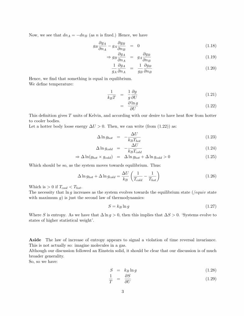
Now, we see that dnA = −dnB (as n is fixed.) Hence, we have

gB∂gA∂nA

− gA∂gB∂nB

= 0 (1.18)

⇒ gB∂gA∂nA

= gA∂gB∂nB

(1.19)

1gA

∂gA∂nA

=1gB

∂gB∂nB

(1.20)

Hence, we find that something is equal in equilibrium.We define temperature:

1kBT

=1g

∂g

∂U(1.21)

=∂ ln g∂U

(1.22)

This definition gives T units of Kelvin, and according with our desire to have heat flow from hotterto cooler bodies.Let a hotter body loose energy ∆U > 0. Then, we can write (from (1.22)) as:

∆ ln ghot = − ∆UkBThot

(1.23)

∆ ln gcold = − ∆UkBTcold

(1.24)

⇒ ∆ ln(ghot × gcold) = ∆ ln ghot + ∆ ln gcold > 0 (1.25)

Which should be so, as the system moves towards equilibrium. Thus:

∆ ln ghot + ∆ ln gcold =∆UkB

(1

Tcold− 1Thot

)(1.26)

Which is > 0 if Tcool < Thot.The necessity that ln g increases as the system evolves towards the equilibrium state (/equiv statewith maximum g) is just the second law of thermodynamics:

S = kB ln g (1.27)

Where S is entropy. As we have that ∆ ln g > 0, then this implies that ∆S > 0. ‘Systems evolve tostates of higher statistical weight’.

Aside The law of increase of entropy appears to signal a violation of time reversal invariance.This is not actually so: imagine molecules in a gas.Although our discussion followed an Einstein solid, it should be clear that our discussion is of muchbroader generality.So, so we have:

S = kB ln g (1.28)1T

=∂S

∂U(1.29)

3

Since we worked hard to get g(n,N), we may as well make use of it. Lets predict the heat capacityof a solid.

S

kB= ln g (1.30)

= (N + n) ln(N + n)− n lnn−N lnN (1.31)1T

=∂S

∂U⇒ 1

T=

1hω

∂S

∂n(1.32)

⇒ ln(N + n

n

)=

hω

kBT(1.33)

⇒ n(T ) =N

ehωkBT − 1

(1.34)

Hence, we have the energy of the solid as a function of temperature: n(T ); remembering thatU = nhω. Hence, we have that the specific heat capacity C is:

C =∂U

∂T

= hω∂n

∂T N

=Nhω hω

kBT 2 ehωkBT

(ehωkBT − 1)2

=NkBX

2eX

(eX − 1)2X ≡ hω

kBT

Hence, for X << 1 (i.e. high T ), we have the Dulong-Petit law: C = NkB. For X >> 1 (i.e. lowT ), we have that C = NkBX

2e−x. So, graphically, we have a curve, starting from 0 at 0, whichincreases to a constant at high temperatures.

2 The Gibbs Factor

We can go further (than the previously closed systems), and figure out the probability that a systemis in a particular quantum state.If the system is closed, then we know the answer: the probability of the system being in any onestate is just 1

g .Generally however, we are interested in systems which are not isolated (i.e. are not closed).Suppose we have a really really big box (denoted the ‘reservior’ R), which is closed; and a smallerbox (our system S), within R, and is allowed to exchange particles and energy with R.At equilibrium, the total number of states available to the system as a whole is:

gT = gS × gR (2.1)

Where gi is the number of accesible states to the system i.In equilibrium, gT is a maximum. As gT (US , NS) we can hence write its differential:

dgT = 0 (2.2)

=∂gT∂US

dUs +∂gT∂NS

dNS (2.3)

4

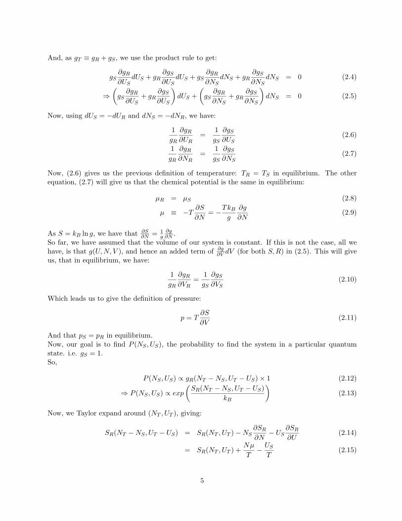
And, as gT ≡ gR + gS , we use the product rule to get:

gS∂gR∂US

dUS + gR∂gS∂US

dUS + gS∂gR∂NS

dNS + gR∂gS∂NS

dNS = 0 (2.4)

⇒(gS∂gR∂US

+ gR∂gS∂US

)dUS +

(gS∂gR∂NS

+ gR∂gS∂NS

)dNS = 0 (2.5)

Now, using dUS = −dUR and dNS = −dNR, we have:

1gR

∂gR∂UR

=1gS

∂gS∂US

(2.6)

1gR

∂gR∂NR

=1gS

∂gS∂NS

(2.7)

Now, (2.6) gives us the previous definition of temperature: TR = TS in equilibrium. The otherequation, (2.7) will give us that the chemical potential is the same in equilibrium:

µR = µS (2.8)

µ ≡ −T ∂S∂N

= −TkBg

∂g

∂N(2.9)

As S = kB ln g, we have that ∂S∂N = 1

g∂g∂N .

So far, we have assumed that the volume of our system is constant. If this is not the case, all wehave, is that g(U,N, V ), and hence an added term of ∂g

∂V dV (for both S,R) in (2.5). This will giveus, that in equilibrium, we have:

1gR

∂gR∂VR

=1gS

∂gS∂VS

(2.10)

Which leads us to give the definition of pressure:

p = T∂S

∂V(2.11)

And that pS = pR in equilibrium.Now, our goal is to find P (NS , US), the probability to find the system in a particular quantumstate. i.e. gS = 1.So,

P (NS , US) ∝ gR(NT −NS , UT − US)× 1 (2.12)

⇒ P (NS , US) ∝ exp(SR(NT −NS , UT − US)

kB

)(2.13)

Now, we Taylor expand around (NT , UT ), giving:

SR(NT −NS , UT − US) = SR(NT , UT )−NS∂SR∂N− US

∂SR∂U

(2.14)

= SR(NT , UT ) +Nµ

T− US

T(2.15)

5

Neglecting terms in higher differentials, as reservior is big enough, then its temperature T andchemical potential µ are independant of NS , US . So, we have:

P (NS , US) ∝ exp(SR(NT , UT )

kB+NSµ

kBT− USkBT

)(2.16)

Now, we notice that the first term in the exponential is a constant (or assumed to be so constantthat it is!); also, we now drop the subscripts, and write that US = εS = ε. This gives us:

P (N, ε) ∝ exp(Nµ− εkBT

)(2.17)

Which is known as the Gibbs distribution function.Notice, that if N is fixed, then the Nµ

kBTterm is another constant, and we have that:

P (ε) ∝ exp(− ε

kBT

)(2.18)

Which is the Boltzmann distribution function, we saw last year.To use the probability properly, we must normalise it. That is:∑

N

∑ε

P (N, ε) = 1 (2.19)

So, to do this, we define the grand partition function Z:

Z(µ, T ) ≡∑N

∑ε

exp

(Nµ− εkBT

)(2.20)

So that we now have the probability to find the system as a whole, in a particular state with energyε, and number of particles N , is given by:

P (N, ε) =exp

(Nµ−εkBT

)Z

(2.21)

Note, if the system has more than one type of particle, then the exponent changes thus:

exp

(Nµ− εkBT

)→ exp

(N1µ1 +N2µ2 + . . .− ε

kBT

)(2.22)

We can compute the average, in the usual way:

〈X〉 =∑

PiXi (2.23)

=∑N,ε

exp(Nµ−εkBT

)Z

X(N, ε) (2.24)

6

2.0.1 Example: CO Poisoning

Suppose that our system of interest is a Haemoglobin molecule, in one of 3 states: unbound (1);bound to O2 (2); bound to CO (3).So, we can write the particle numbers, for each state, in terms of (NHb, NO2 , NCO), with theirassociated energies (given)

• (1) : (1, 0, 0) ε1 = 0

• (2) : (1, 1, 0) ε2 = −0.7eV

• (3) : (1, 0, 1) ε3 = −0.85eV

The chemical potentials are: µHb =dont care! µO2 = −0.6eV , µCO = −0.7eV (again, values given).T = 310K.So, to calculate Z, we have:

Z = exp

(NHb

1 µHb +NO21 µO2 +NCO

1 µCO − ε1kBT

)(2.25)

+ exp

(NHb

2 µHb +NO22 µO2 +NCO

2 µCO − ε2kBT

)(2.26)

+ exp

(NHb

1 µHb +NO23 µO2 +NCO

3 µCO − ε3kBT

)(2.27)

= eµHb/kBT + e(µHb+µO2+0.7eV )/kBT + e(µHb+µCO+0.85eV )/kBT (2.28)

= 161 (2.29)

Hence, we can write what the probability of each state (1), (2) or (3) is, of occuring:

• (1): Hb is unbound: P1 = eµHb/kBT

Z = 1161 .

• (2): Hb is bound to O2: 2 = e(µHb+µO2

+0.7eV )/kBT

Z = 40161 = 25%.

• (3): Hb is bound to CO: P3 = e(µHb+µCO+0.85eV )/kBT

Z = 120161 = 75%

2.1 My Grand Partition Function

I find the following formula easier to use, to write the probability of finding the system in a statewith energy εj , with N particles:

P (N, εj) =eεj/kT

∏i eNiµi/kT

ZThus, the grand partition function Z is the sum over all possible energy states as well:

Z =∑j

eεj/kT∏i

eNiµi/kT

7

3 Identical Particles

We shall be looking at cases where the ‘system’ is a ‘bunch of particles’. We need to be able tocount quantum states for such system. We start with a simple system.

3.1 Distinguishable Particles

If we have 2 distinguishable particles (A,B), and 2 accesible quantum states (ε1, ε2), and if theparticles are distinguishable, then we can have 4 configurations: (AB, 0), (0, AB), (A,B), (B,A).Hence, 4 allowed states of the system.

3.2 Indistinguishable Particles

If we have again 2 accesible states, but 2 identical particles, we now have that the possible config-urations are: (AA, 0), (0, AA), (A,A). Hence, 3 allowed states. This is the case if we allow the twoparticles to be in the same state at the same time, We denote these types of particles bosons.

The other possibility is that we dont allow the two particles to be in the same state. Hence, wehave that the only configuration is (A,A). We denote these types of particles fermions. That thereis only one state allowed, is a consequence of the Pauli Principle. Which we shall now derive.

3.3 Pauli Principle

Let φi(x) be an energy eigenstate for a single particle in the system, so that:

H(x)φi(x) = Eiφi(x)

If our two particles do not interact, then φi(x)φj(y) is an energy eigenstate of the two particlesystem, with E = Ei + Ej :[

H(x) + H(x)]φi(x)φj(y) = Eiφi(x)φj(y) + Ejφi(x)φj(y)

If the particles are indistinguishable, then no observable can depend upon which particle is where.Hence, we have that observables should be unchanged if we swap the positions x↔ y:⟨

O⟩

=∫ψ∗(x, y)O(x, y)ψ(x, y)dτ

Should be unchanged under the swap.Recall that any linear combination of 2 eigenstates is also an eigenstate with the same eigenvalue.So, we want a linear combination:

aφi(x)φj(y) + bφi(y)φj(x) = ψij(x, y)

⇒[H(x) + H(x)

]ψij(x, y) = (Ei + Ej)ψij(x, y)

8

Now, we want:|ψij(x, y)|2 = |ψij(y, x)|2

This implies that:ψij(x, y) = eiαψij(y, x)

Where swaping over the spatial coordinates has the effect of picking up some phase eiα. Now, if weswap back:

ψij(x, y) = eiαeiαψij(x, y)⇒ e2iα = 1⇒ eiα = ±1

So, we have that:ψij(x, y) = ±ψij(y, x)

Now, there are two linear combinations of φi(x)φj(y) and φi(y)φj(x) which satisfy this requirement:

ψij(x, y) = φi(x)φj(y)± φi(y)φj(x) (3.1)

If the positive sign is taken, then the wavefunction is symmetric (under interchange of two identicalparticles). We classify this type as being bosons. If the negative sign is taken, then the wavefunctionis anti-symmetric, and we classify these as fermions.We see that the Pauli principle is a direct consequence of the symmetry property for fermions:If we have 2 identical fermions in the same state i, then:

ψii(x, y) = φi(x)φi(y)− φi(y)φi(x) = 0⇒ |ψii(x, y)|2 = 0

That is, there is no probability for the system to be found in such a state. Therefore, two identicalfermions can not be in the same quantum state. There is no such problem for bosons.This is actually a pretty weird conclusion. If we have the idea that an electrons wavefunction isnever zero (just really small) anywhere, then any two electrons in the universe must be considereddependantly, and we must conclude that these two electrons can never be in the exact same state.That is, we cannot treat an electron sitting on the earth independantly to one on the other sideof the galaxy. These two electrons simply can never be in the same state. We end up concludingthat they are allowed to sit very very close to being in the same state, but not quite. This can beshown in potential well arguments. There is a very fine difference between the ground state of twoelectrons whose wavefunctions overlap.

We ought to conclude by stating that bosons have integer spin, and fermions half-integer. This isproved using relativistic quantum mechanics, and is hard to do!If a collection of particles have an odd number of fermions, then the system is fermionic; evennumber of fermions gives a bosonic system.

4 The Bose-Einstein & Fermi-Dirac Distributions

We now focus on an ideal gas of fermions or bosons.We recall that the Gibbs distribution gives the probability to find the system S in a single quantum

9

state.A single state of S is specified by the set {ni, εi}; where ni is the number of particles in the energylevel εi. So:

P ({ni, εi}) =exp[µ(n1 + n2,+ . . .)/kT − (ε1n1 + ε2n2 + . . .)/kT ]∑

n1,n2,...exp[µ(n1 + n2,+ . . .)/kT − (ε1n1 + ε2n2 + . . .)/kT ]

(4.1)

=en1(µ−ε1)/kT en2(µ−ε2)/kT . . .∑

n1en1(µ−ε1)/kT

∑n2en2(µ−ε2)/kT . . .

(4.2)

= P1(n1)P2(n2) . . . (4.3)

Where:

Pi(ni) ≡eni(µ−εi)/kT∑nieni(µ−εi)/kT

Thus, Pi(ni) is the probability to find ni particles in energy level εi. What we have done is to showthat the probability to find the system in a particular state is just the product of the probabilitiesof finding a particular number of particles in the particular state.Now, we can figure out the mean number of particles in a particular energy level:

〈n(εi)〉 =∑

Pini

It is the calculation of this sum which we now consider:

4.1 Fermi-Dirac Distribution

Here, we just condsider the fermionic case. We know that we can only have either one or zeroparticles in each state. Thus, the sum over n is just for n = 0, 1. Hence:

〈n(ε)〉FD =∑n=0,1

P (n)n (4.4)

=1× 0 + e(µ−ε)/kT

1 + e(µ−ε)/kT (4.5)

=1

1 + e(ε−µ)/kT(4.6)

⇒ 〈n(ε)〉FD =1

1 + e(ε−µ)/kT(4.7)

Where 〈n(ε)〉FD is called the Fermi-Dirac Distribution.

4.2 Bose-Einstein Distribution

Here, we can have any number of particles in each state. Hence:

〈n(ε)〉BE =0 + e(µ−ε)/kT + 2e2(µ−ε)/kT + . . .

1 + e() + e2() + . . .(4.8)

10

Now, if we define:a ≡ e(µ−ε)/kT

We see that the denominator is a geometric series:

1 + a+ a2 + a3 + . . . =1

1− a

And that the top is:

a+ 2a2 + 3a3 + . . . (4.9)= a(1 + 2a+ 3a2 + . . .) (4.10)

= a( dda(1 + a+ a2 + . . .)) (4.11)

= a(1−a)2 (4.12)

Hence, we have that:

〈n(ε)〉BE =a

(1−a)2

11−a

(4.13)

=1

1a − 1

(4.14)

=1

e(ε−µ)/kT − 1(4.15)

⇒ 〈n(ε)〉BE =1

e(ε−µ)/kT − 1(4.16)

Where 〈n(ε)〉BE is called the Bose-Einstein Distribution.

4.3 Spin Multiplicity

In a gas of particles with spin s, the mean number of particles per state is hence given by:

〈n(ε)〉 =2s+ 1

e(ε−µ)/kT ± 1

5 Classical Limit

We have the classical limit when:〈n(ε)〉 << 1 ∀ε

i.e. we have that:

〈n(ε)〉 ≈ exp(µ− εkT

)Using the approximation, we can start to calculate things.

11

Figure 1: Graph showing how the three distributions change. Notice that the Fermi-Dirac distri-bution stays below 1.

5.1 Chemical Potential µ

We can develop insight into µ by computing the mean number of particles in our system as a whole.Suppose we have N particles, within a big cube, with sides length L. Our system is within the bigcube. So, we have:

N =∑i

〈n(εi)〉

=∑i

exp

(µ− εkT

)Now, let us attempt the summation.We need the single particle energy levels for (non-interacting) particles in a box of side L. To dothis, just solve the Schrodinger equation, to find:

ε(n1, n2, n3) =h2π2

2mL2(n2

1 + n22 + n2

3)

Where the integers ni run from 1, 2, 3, . . . ,∞. Hence we have that the total number of particles inthe system is:

N =∑

n1,n2,n3

exp

(µ− ε(n1, n2, n3)

kT

)To find typical values of n1, n2, n3 via noting that we have that ε = kT ; hence:

n21 + n2

2 + n23 ≈

kT2mL2

h2π2

Now, if L = 1m & m = 10−26kg, we have that n1, n2, n3 ≈ 1019/2.

12

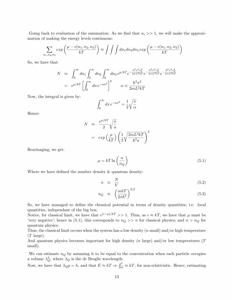
Going back to evaluation of the summation: As we find that ni >> 1, we will make the approxi-mation of making the energy levels continuous:∑

n1,n2,n3

exp

(µ− ε(n1, n2, n3)

kT

)≈∫ ∫ ∫

dn1dn2dn3 exp

(µ− ε(n1, n2, n3)

kT

)So, we have that:

N ≈∫ ∞

0dn1

∫ ∞0

dn2

∫ ∞0

dn3 eµ/kT e−

h2π2n21

2mL2kT e−h2π2n2

22mL2kT e−

h2π2n23

2mL2kT

= eµ/kT[∫ ∞

0dn e−αn

2

]3

α ≡ h2π2

2mL2kT

Now, the integral is given by: ∫ ∞0

dx e−αx2

=12

√π

α

Hence:

N ≈ eµ/kT

2

√π

α

= exp( µ

kT

)(12

√2mL2kT

h2π

)3

Rearinaging, we get:

µ = kT ln(n

nQ

)(5.1)

Where we have defined the number density & quantum density:

n ≡ N

V(5.2)

nQ ≡(mkT

2πh2

)3/2

(5.3)

So, we have managed to define the chemical potential in terms of density quantities; i.e. localquantities, independant of the big box.Notice, for classical limit, we have that e(ε−µ)/kT >> 1. Thus, as ε ≈ kT , we have that µ must be‘very negative’; hence in (5.1), this corresponds to nQ >> n for classical physics; and n > nQ forquantum physics.Thus, the classical limit occurs when the system has a low density (n small) and/or high temperature(T large).And quantum physics becomes important for high density (n large) and/or low temperatures (Tsmall).

We can estimate nQ by assuming it to be equal to the concentration when each particle occupiesa volume λ3

Q, where λQ is the de Broglie wavelength.

Now, we have that λQp = h, and that E ≈ kT ⇒ p2

2m ≈ kT , for non-relativistic. Hence, estimating

13

gives: p ≈√mkT . Therefore, λQ ≈ h√

mkT. Now, we want nQ ≈ 1

λ3Q

, and we have hence acheived

the previous value of nQ.Hence, we may say that the quantum density nQ is that at which particles occupy boxes the size oftheir de Broglie wavelengths.

Comments

• Dont forget the spin multiplicity factor. If the gas particles have spin s, thenn = (2s+ 1)exp(µ/kT )nQ ⇒ µ = kT ln(n/(2s+ 1)nQ).

• Actual values of µ depend of what we choose as the zero of the energy scale. If ε = ε0 +ε(n1, n2, n3), then a change of µ → µ + ε0 would keep everything the same. So µ = ε0 +kT ln(n/nQ).

We have assumed that the gas so far is monoatomic. Now, if we give the system a set {j} ofinternal quantum numbers (e.g angular momentum), then we have that we can find the new chemicalpotential µ. We proceed by finding the average number of particles (in total) in the system, whichis just the sum over probabilities to find a number of particles in an energy state:

N =∑i

ni

=∑i

eµ−εikT

= eµ/kT∑i

e−εi/kT

= eµ/kTZ

=n

nQZ

Where we have defined the partition function Z ≡∑

i e−εi/kT . Now, from the definition n = N

L3 .Hence:

N =NZ

L3nQ(5.4)

⇒ Z = nQL3 (5.5)

So, now, if we introduce internal degrees of freedom, we introduce another energy term εj ; hence:

N = eµ/kT∑i

e−εi/kT∑j

e−εj/kT

⇒ n =N

L3= eµ/kT

∑i e−εi/kT

L3

∑j

e−εj/kT

⇒ n = eµ/kTZ

L3Zint

⇒ µ = kT ln(

n

nQZint

)14

Hence, we see that if we introduce internal motion of the particles, described by the internal partitionfunction Zint, the chemical potential is given by:

µ = kT ln(

n

nQZint

)(5.6)

5.1.1 Internal Energy & Heat Capacity

We know that the internal energy U is given by the sum over the different states, where each stateis the mean number of particles in each energy level (state):

U =∑i

〈ni〉εi

=∑i

e(µ−εi)/kT εi

= eµ/kT∑i

e−εi/kT εi

=n

nQ

∑i

e−εi/kT εi

=N

L3

L3

Z

∑i

e−εi/kT εi

=N

Z

∑i

e−εi/kT εi

Where we have used that Z = nQL3 and n = N/L3. Now, we notice that the last expression is

equal to the differential of the logarithm of the partition function:

⇒ U = NkT 2∂ lnZ∂T

= NkT 2 ∂

∂Tln(nQL3)

=32NkT

After doing the differentiation, and subbing in for nQ.We can also compute the heat capacity:

CV =∂U

∂T=

32Nk

Where we have now been able to reproduce last years results.

5.2 Entropy of an Ideal Gas

We must count all accesible quantum states. But it is not clear how to do that for a system withvariable particle number and energy.We can compute the mean entropy by considering the following situation:

15

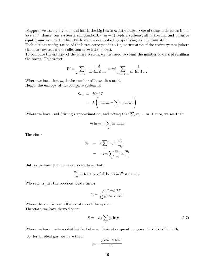
Suppose we have a big box, and inside the big box is m little boxes. One of these little boxes is our‘system’. Hence, our system is surrounded by (m− 1) replica systems, all in thermal and diffusiveequilibrium with each other. Each system is specified by specifying its quantum state.Each distinct configuration of the boxes corresponds to 1 quantum state of the entire system (wherethe entire system is the collection of m little boxes).To compute the entropy of the entire system, we just need to count the number of ways of shufflingthe boxes. This is just:

W =∑

m1,m2,...

m!m1!m2! . . .

= m!∑

m1,m2,...

1m1!m2! . . .

Where we have that mi is the number of boxes in state i.Hence, the entropy of the complete system is:

Sm = k lnW

= k

(m lnm−

∑i

mi lnmi

)

Where we have used Stirling’s approximation, and noting that∑

imi = m. Hence, we see that:

m lnm =∑i

mi lnm

Therefore:

Sm = k∑i

mi lnm

mi

= −km∑i

mi

mlnmi

m

But, as we have that m→∞, so we have that:

mi

m= fraction of all boxes in ith state = pi

Where pi is just the previous Gibbs factor:

pi =e(µNi−εi)/kT∑e(µNi−εi)/kT

Where the sum is over all microstates of the system.Therefore, we have derived that:

S = −kB∑i

pi ln pi (5.7)

Where we have made no distinction between classical or quantum gases: this holds for both.

So, for an ideal gas, we have that:

pi =e(µNi−Ei)/kT

Z

16

Where we have that:

Ni = n1 + n2 + n3 + . . .

Ei = n1ε1 + n2ε2 + n3ε3 + . . .

Hence, let us compute Z generally.

Z =∑{ni}

en1(µ−ε1)/kT × en2(µ−ε2)/kT × . . .

Where we have a summation over occupancies over single particle states. Hence, we can show thatthis summation is the same as the product of the corresponding factors:

Z =∏{εi}

(1 + e(µ−εi)/kT + e2(µ−εi)/kT + . . .

)(5.8)

=∏{εi}

∑{nj}

(enj(µ−εi)/kT

)(5.9)

And we see that the sum is just the standard∑∞

i=0 xi = 1

1−x , to give:

Z =∏{εi}

11− e(µ−εi)/kT

Taking the logarithm:

lnZ = ln∏{εi}

11− e(µ−εi)/kT

=∑{εi}

ln1

1− e(µ−εi)/kT

= −∑{εi}

ln 1− e(µ−εi)/kT

Hence, we see that, for bosons, this sum is unrestricted; so:

lnZboson = −∑{εi}

ln(

1− e(µ−εi)/kT)

(5.10)

For fermions, the sum in (5.9) is just for nj = 0, 1; and is hence trivial, and we find that, forfermions:

lnZfermion =∑{εi}

ln(

1 + e(µ−εi)/kT)

(5.11)

In the classical limite(µ−ε)/kT << 1

We have, using ln(1 +X) ≈ X, that both the boson and fermion grand partition functions are thesame:

lnZclassical ≈∑i

e(µ−εi)/kT = eµ/kT∑i

e−ε/kT

17

i.e. Zclassical ≈ Zboson ≈ Zfermion in the classical limit.Hence, in the classical limit, we can compute S = −k

∑i pi ln pi, where i is over the states of the

gas. Below, j are the single particle energy levels:

S = −k∑i

pi ln pi

= −k∑i

e(µNi−Ei)/kT

Zlne(µNi−Ei)/kT

Z

= −k∑i

e(µNi−Ei)/kT

Z

(ln e(µNi−Ei)/kT − lnZ

)

= −k∑i

e(µNi−Ei)/kT

Z

µNi − EikT

− eµ/kT∑j

e−εj/kT

= −k

(µ

kT

∑i

piNi −1kT

∑i

piEi − eµ/kTZ

)

= −k(µN

kT− U

kT− Zeµ/kT

)Where we have used the partition function Z =

∑j e−εj/kT , and that the expressions for the average

particle number and energy were written:∑

iNipi = 〈N〉 = N and∑

iEipi = 〈E〉 = U .Now, we have previously derived that µ = kT ln n

nQ, and Z = nQV . Hence, we have:

S = −k(N ln

n

nQ− U

kT− n

nQnQV

)If we put:

U =32NkT nV = N

Then:

S = Nk

(52

+ lnnQn

)(5.12)

Which is known as the Sackur-Tetrode equation.

Even though this calculation has been done in the classical limit, we have had to use the quantumphysics of identical particles to get this expression correct. A classical result, built on quantumphysics.

18

We can now easily compute the pressure and Cp. We start with pressure:

p = T∂S

∂V

)N,U

= NkT∂

∂V

(lnnQ + ln

V

N

)N,U

= NkT∂

∂VlnV

=NkT

V⇒ pV = NkT

Where we have used that nQ(T ) only, and that if we fix N and U , we therefore fix T . And finally,the heat capacity at constant pressure:

Cp = T∂S

∂T

)p,N

= NkT

[∂

∂T

(lnNkT

p

)+

32

1T

]=

52NkT

Notice, we have also recovered a previously known result: Cp − CV = NkT .

6 Fermi Gases

We shall focus on a non-interacting gas of spin-12 particles. At sufficiently low temperatures, quan-

tum effects are crucial. So it remains to show when we we can use the classical limit, and whenquantum physics becomes important.Examples of such systems are:

• Electrons in a metal ‘free electron theory’;

• 3He atoms;

• Electrons in white dwarf stars;

• Neutrons in neutron stars;

• Nucleons in a nucleus.

Example We will show that free electrons in a metal at room temperature will be in the quantumregime, whereas hydrogen at STP will not.We know we need to use quantum physics if n ≥ nQ.Consider the electrons first:

19

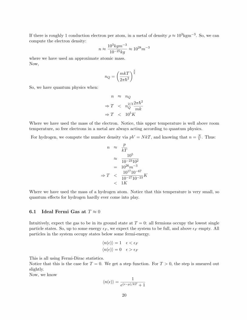
If there is roughly 1 conduction electron per atom, in a metal of density ρ ≈ 103kgm−3. So, we cancompute the electron density:

n ≈ 103kgm−3

10−25kg≈ 1028m−3

where we have used an approximate atomic mass.Now,

nQ =(mkT

2πh2

) 32

So, we have quantum physics when:

n ≈ nQ

⇒ T < n2/3Q

2πh2

mk⇒ T < 105K

Where we have used the mass of the electron. Notice, this upper temperature is well above roomtemperature, so free electrons in a metal are always acting according to quantum physics.

For hydrogen, we compute the number density via pV = NkT , and knowing that n = NV . Thus:

n ≈ p

kT

≈ 105

10−23102

= 1026m−3

⇒ T <101710−67

10−2710−23K

< 1K

Where we have used the mass of a hydrogen atom. Notice that this temperature is very small, soquantum effects for hydrogen hardly ever come into play.

6.1 Ideal Fermi Gas at T ≈ 0

Intuitively, expect the gas to be in its ground state at T = 0: all fermions occupy the lowest singleparticle states. So, up to some energy εF , we expect the system to be full, and above εF empty. Allparticles in the system occupy states below some fermi-energy.

〈n(ε)〉 = 1 ε < εF

〈n(ε)〉 = 0 ε > εF

This is all using Fermi-Dirac statistics.Notice that this is the case for T = 0. We get a step function. For T > 0, the step is smeared outslightly.Now, we know

〈n(ε)〉 =1

e(ε−µ)/kT + 1

20

If ε > µ, then (under T = 0), we have that 〈n〉 = 0.Similarly, if ε < µ, then 〈n〉 = 1.Hence, we have the interpretation that the Fermi-energy εF is the value of the chemical potential µat T = 0.

εF ≡ µ(T = 0) (6.1)

At T = 0, all single particle states below εF are filled, whilst all those above are empty.We denote a system at T ≈ 0 as being a degenerate Fermi gas, and one at T = 0 an ideal Fermigas.So a gas of fermions that is cold enough so that nearly all states below εF are filled, and nearly allstates above is called a degenerate fermi gas. This is just reiterating what has previously been said.Now, if the gas is non-relativistic, we have the relations:

εF ≡p2F

2m=h2k2

F

2mkBTF ≡ εF

Where we have thus defined the Fermi temperature TF , Fermi momentum pF , and Fermi wavenum-ber kF in terms of the Fermi energy εF . Notice that we must distinguish between Boltzmann factorkB and Fermi wavenumber kF .If the gas is ultra-relativistic (m0 << p):

εF = cpF

= hckF

Clearly, εF must depend upon the number of particles N , so that we have that the number ofparticles below εF is N .

Example Compute εF for a 2D non-relativistic electron gas containing N electrons in an area A.

Let us construct a box, of side length L, so that L2 = A. Then we have the Schrodinger equation,with its solution:

− h2

2m∇2ψ = εψ

⇒ ψ ∝ sinn1πx

Lsin

n2πy

L

ε =h2π2

2mL2(n2

1 + n22)

Where n1, n2 > 0 and are integers.We must remember that for each state, we can have two spin-half electrons.Hence, we want N to be twice the total number of single particle states with ε ≤ εF :

n21 + n2

2 ≤εF 2mL2

h2π2

21

It is more convenient to work in terms of wavevectors k = (kx, ky), so that ψ ∝ sin(kxx) sin(kyy).We obviously have that kx ≡ n1π

L and ky ≡ n2πL . Hence, we can write the condition as:

h2k2

2m≤ εF

Where k2 = k2x + k2

y.Notice that the distance between adjacent states in k-space is just π

L , and hence that the areaoccupied by one state is

(πL

)2.Now, we want to know how many states there are with k2

x + k2y ≤ k2

F . That is, the area of thequarter-circle of radius k2

F , in k-space.Thus, the number of electrons (which is twice the number of single particle energy states) in suchan area is given by N = 2 × area of quarter cricle / area occupied by each state:

N = 2πk2F

4(πL

)2⇒ k2

F =N

L22π

= 2πn

Where n is just the number density n ≡ NL2 .

6.2 Density of States

Considering a 2D gas of Fermions:Suppose we have an annulus, in the positive quarter of k-space. How many states reside here?The number of states is obviously the area of the annulus, divided by the area of one state.If the number of states is dn, and the annulus is k → dk, then the area of the total circular annulusis 2πkdk, and hence of the quarter annulus is 1

42πkdk. We already have that the area taken upby one state is

(πL

)2. Now, its important to note that we have been talking about the number ofstates. If we have a spin s-particle, there is allowed to be 2s + 1 such particles in each state. Wehence need to multiply any answer by the number of particles allowed in each state. For electrons,s = 1

2 , so everything is multiplied by 2. We hence can write:

dn = 2142πkdk(

πL

)2=

kdkL2

π

⇒ dn

dk=

kL2

π

We hence have that dndk is the density of states in k-space. The number of states dn per unit of k.

We can now rederive the Fermi-energy for our 2D electron gas.The number of particles N below the Fermi-wavenumber kF is the same as the total number of

22

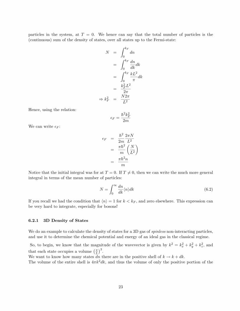
particles in the system, at T = 0. We hence can say that the total number of particles is the(continuous) sum of the density of states, over all states up to the Fermi-state:

N =∫ kF

0dn

=∫ kF

0

dn

dkdk

=∫ kF

0

kL2

πdk

=k2FL

2

2π

⇒ k2F =

N2πL2

Hence, using the relation:

εF =h2k2

F

2mWe can write εF :

εF =h2

2m2πNL2

=πh2

m

(N

L2

)=

πh2n

m

Notice that the initial integral was for at T = 0. If T 6= 0, then we can write the much more generalintegral in terms of the mean number of particles:

N =∫ ∞

0

dn

dk〈n〉dk (6.2)

If you recall we had the condition that 〈n〉 = 1 for k < kF , and zero elsewhere. This expression canbe very hard to integrate, especially for bosons!

6.2.1 3D Density of States

We do an example to calculate the density of states for a 3D gas of spinless non-interacting particles,and use it to determine the chemical potential and energy of an ideal gas in the classical regime.

So, to begin, we know that the magnitude of the wavevector is given by k2 = k2x + k2

y + k2z , and

that each state occupies a volume(πL

)3.We want to know how many states dn there are in the positive shell of k → k + dk.The volume of the entire shell is 4πk2dk, and thus the volume of only the positive portion of the

23

shell is 184πk2dk. Hence, we can write:

dn =184πk2dk(

πL

)3=

L3k2dk

2π2

⇒ dn

dk=

k2L3

2π2

=k2V

2π2

Thus, we have derived the density of states for a 3D gas of spinless fermions.To get the chemical potential, we need to continue to solve N for µ, via:

N =∫ ∞

0

dn

dk〈n〉dk

Now, we have that

〈n〉 =1

e(ε−µ)/kBT + 1Which, in the classical limit (notice that the classical limit dosent care if its a boson or fermion)reduces to:

〈n〉 = e(µ−ε)/kBT

Hence:

N =∫ ∞

0

V k2

2π2dke−ε/kBT eµ/kBT

Notice, we also have that ε(k) = h2k2

2m , so the integral is pretty hard to do. So, an alternativemethod, is to change variable, so right from the start, we have:

N =∫ ∞

0

dn

dε〈n〉dε

Hence, to do things using this method, we need the density of states in ε-space, as opposed tok-space. We can do this by chain rule:

dn

dε=

dn

dk

dk

dε

=k2V

2π2

12

√2mεh2

=2mεh2

12

√2mεh2

=V m3/2

√2

2π2h3

√ε

Where we have made use of ε = h2k2

2m ⇒ k =√

2mεh2 , and the original density of states dn

dk . We canimmediately see that, for a non-relativistic gas:

dn

dε∝√ε

24

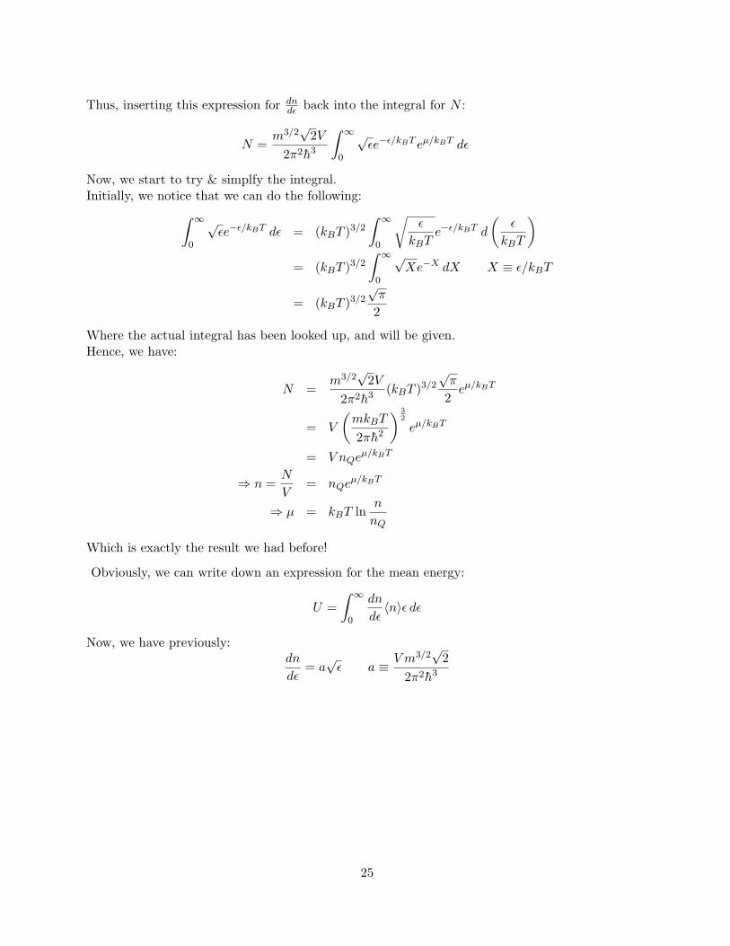
Thus, inserting this expression for dndε back into the integral for N :

N =m3/2

√2V

2π2h3

∫ ∞0

√εe−ε/kBT eµ/kBT dε

Now, we start to try & simplfy the integral.Initially, we notice that we can do the following:∫ ∞

0

√εe−ε/kBT dε = (kBT )3/2

∫ ∞0

√ε

kBTe−ε/kBT d

(ε

kBT

)= (kBT )3/2

∫ ∞0

√Xe−X dX X ≡ ε/kBT

= (kBT )3/2

√π

2

Where the actual integral has been looked up, and will be given.Hence, we have:

N =m3/2

√2V

2π2h3 (kBT )3/2

√π

2eµ/kBT

= V

(mkBT

2πh2

) 32

eµ/kBT

= V nQeµ/kBT

⇒ n =N

V= nQe

µ/kBT

⇒ µ = kBT lnn

nQ

Which is exactly the result we had before!

Obviously, we can write down an expression for the mean energy:

U =∫ ∞

0

dn

dε〈n〉ε dε

Now, we have previously:dn

dε= a√ε a ≡ V m3/2

√2

2π2h3

25

So:

U = a

∫ ∞0

√εe(µ−ε)/kBT ε dε

= b

∫ ∞0

ε3/2e−ε/kBT dε b ≡ aeµ/kBT

= b(kBT )5/2

∫ ∞0

(ε

kBT

)3/2

e−ε/kBT d

(ε

kBT

)= b(kBT )5/2

∫ ∞0

X3/2e−X dX X ≡ ε/kBT

= b(kBT )5/2 3√π

4

=V m3/2

√2

2π2h3 eµ/kBT (kBT )5/2 3√π

4

=V m3/2

√2

2π2h3 (kBT )5/2 3√π

4n

nQ

=V m3/2

√2

2π2h3 (kBT )5/2 3√π

4N

V

(2πh2

mkBT

) 32

=V m3/2

√2k5/2

B T 5/23√πN23/2π3/2h3

2π2h34V m3/2k3/2B T 3/2

=32NkBT

Which again, is a result we previously knew.In these two examples, we have used the ’standard integrals’:∫ ∞

0x3/2e−xdx =

34√π∫ ∞

0

√xe−xdx =

12√π

Which will be given, if needed.

We can use these couple of examples as a prototype for finding the average value of something: addup the average number of particles in a particular state, times the density of particles in a particularstate, multiply by the thing you want the average of. This gives the average of the quantity overthe whole system.So, the average number of particles is given by:

〈N〉 = N =∫ ∞

0

dn

dk〈n〉 dk (6.3)

And the average internal energy of the system:

〈U〉 = U =∫ ∞

0

dn

dk〈n〉ε dk (6.4)

26

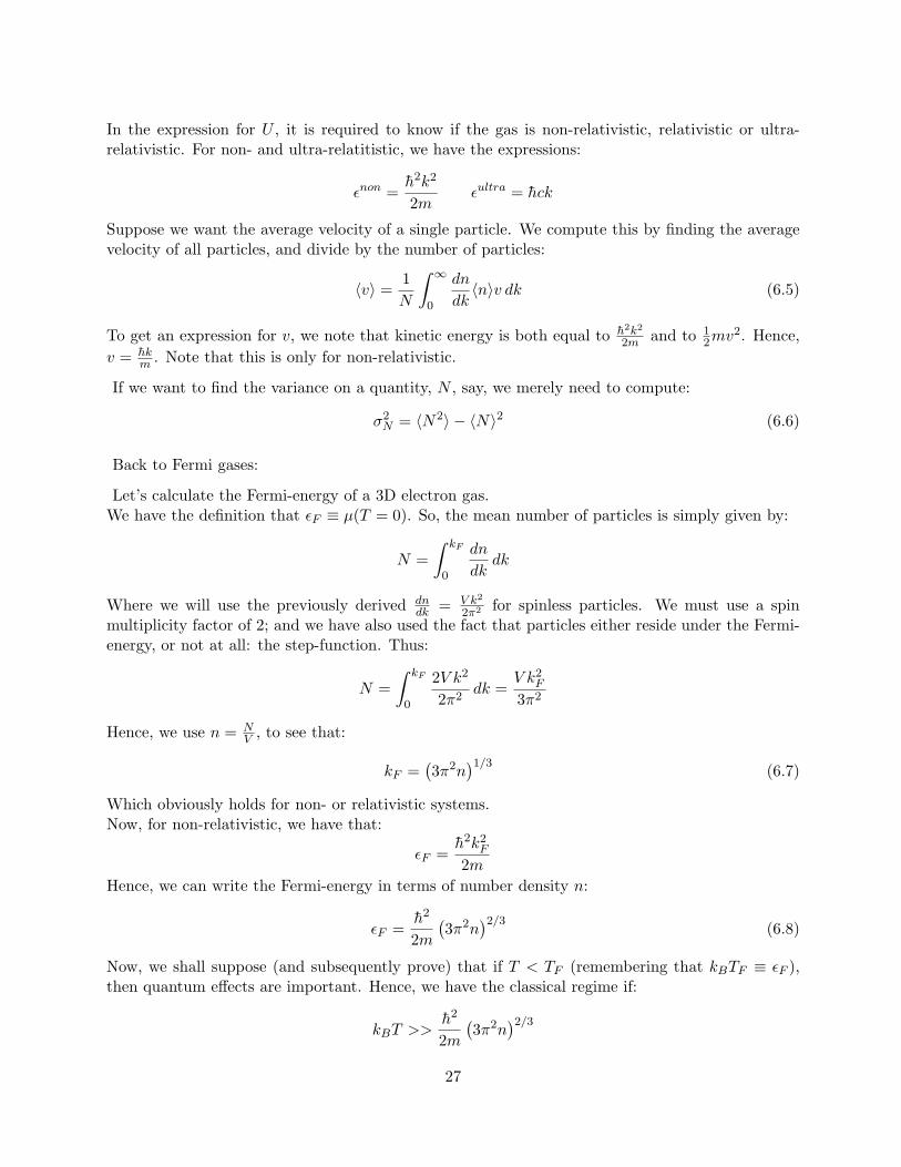
In the expression for U , it is required to know if the gas is non-relativistic, relativistic or ultra-relativistic. For non- and ultra-relatitistic, we have the expressions:

εnon =h2k2

2mεultra = hck

Suppose we want the average velocity of a single particle. We compute this by finding the averagevelocity of all particles, and divide by the number of particles:

〈v〉 =1N

∫ ∞0

dn

dk〈n〉v dk (6.5)

To get an expression for v, we note that kinetic energy is both equal to h2k2

2m and to 12mv

2. Hence,v = hk

m . Note that this is only for non-relativistic.

If we want to find the variance on a quantity, N , say, we merely need to compute:

σ2N = 〈N2〉 − 〈N〉2 (6.6)

Back to Fermi gases:

Let’s calculate the Fermi-energy of a 3D electron gas.We have the definition that εF ≡ µ(T = 0). So, the mean number of particles is simply given by:

N =∫ kF

0

dn

dkdk

Where we will use the previously derived dndk = V k2

2π2 for spinless particles. We must use a spinmultiplicity factor of 2; and we have also used the fact that particles either reside under the Fermi-energy, or not at all: the step-function. Thus:

N =∫ kF

0

2V k2

2π2dk =

V k2F

3π2

Hence, we use n = NV , to see that:

kF =(3π2n

)1/3 (6.7)

Which obviously holds for non- or relativistic systems.Now, for non-relativistic, we have that:

εF =h2k2

F

2mHence, we can write the Fermi-energy in terms of number density n:

εF =h2

2m(3π2n

)2/3 (6.8)

Now, we shall suppose (and subsequently prove) that if T < TF (remembering that kBTF ≡ εF ),then quantum effects are important. Hence, we have the classical regime if:

kBT >>h2

2m(3π2n

)2/327

Or, that:

n <<

(2mkBTh2

)3/2 13π2

(6.9)

Now, we have that the quantum concentration nQ is given by:

nQ =(

2mkBT2πh2

)3/2

Hence, we see that (6.9) is equivalent to:

n << nQ8

3√π

Hence, we have that n << nQ for classical. Which is our previous definiton, but derived by statingthat T >> TF for classical.

Now, let’s calculate the internal energy of a non-relativistic 3D gas of electrons. We have straightaway that:

U =∫ kF

0

V k2

π2

h2k2

2mdk =

V

π2

h2

2mk2F

5

Now, from (6.7), we have:

kF =(3π2n

)1/3 ⇒ N =V k3

F

3π2

Hence,

U =35Nh2k2

F

2m

But we also have the relation that εF = h2k2F

2m . Hence:

U =35NεF (6.10)

Now, if we want to calculate the pressure p, we initially start by writing:

dU = TdS − pdV

Which, at T = 0, reduces to:

p = − ∂U

∂V

)N

Hence:

p = − ∂

∂V

35NεF

= −35N∂εF∂V

Where we can do the differentiation:∂εF∂V

= −23εFV

28

Hence:p =

25NεFV

=25nεF

Which we can rearrange into the equation of state for a Fermi-gas at low temperature:

pV =25NεF (6.11)

This is the equivalent of pV = NkBT .

To get CV , we take:

CV =∂U

∂T

)V

= 0

At T = 0, as U is independant of T at 0. This is a little useless, as it does not tell us what happensas T → 0. To find out this behavior, we need to do some small T corrections to U . To do thisproperly, we need to evaluate the integral:

U =∫ ∞

0

dn

dk

1e(ε−µ)/kBT + 1

ε dk

Which is hard.We can estimate the correction by saying that only particles within kBT of εF move. So, the numberof excited particles is:

kBT

εFN

So, additional energy is of the order:kBT

εFNkBT

Hence, U needs to be corrected by this factor:

U =35NεF + α

(kBT )2

εFN

Where α is some constant. If this correction is done exactly, one finds that α = π2

4 . Hence, if wenow calculate CV using this corrected version of U , we find:

CV =∂U

∂T

)V

=Nk2

BTπ2

2εF

6.2.2 Low T Corrections to N,U

Now, we have that:

N =∫ ∞

0

dn

dε〈n〉 dε

=∫ ∞

0

dn

dε

1e(ε−µ)/kBT

dε

U =∫ ∞

0

dn

dε

1e(ε−µ)/kBT

ε dε

29

We have previously derived that:dn

dε=

32Nε−3/2F ε1/2

So, to solve these integrals, we have objects of the form:

I =∫ ∞

0

f(ε)e(ε−µ)/kBT

dε

Now, we must be able to write the answer in terms of:

I =∫ µ

0f(ε) dε+ corrections in T → 0

So, we want to try to get our integral in that form.Suppose we define:

z ≡ ε− µkBT

Hence, we see that z(ε = 0) = −µ/kBT , and ε = kBTz + µ. I will now omit the subscript B fromBoltzmanns constant. Hence, we have:

I = kT

∫ ∞−µ/kT

f(zkT + µ)ez + 1

dz

Which we can split into 2 integrals:

I = kT

∫ 0

−µ/kT

f(zkT + µ)ez + 1

dz + kT

∫ ∞0

f(zkT + µ)ez + 1

dz

And we can invert the firsts limits:

I = kT

∫ µ/kT

0

f(µ− zkT )e−z + 1

dz + kT

∫ ∞0

f(zkT + µ)ez + 1

dz

Now, if we write:1

e−z + 1= 1− 1

ez + 1Then the integral becomes:

I = kT

∫ ∞0

f(zkT + µ)ez + 1

dz + kT

(∫ µ/kT

0f(µ− zkT ) dz −

∫ µ/kT

0

f(µ− zkT )ez + 1

dz)

)

= kT

∫ µ

0f(ε) dε− kT

(∫ µ/kT

0

f(µ− zkT )ez + 1

dz −∫ ∞

0

f(zkT + µ)ez + 1

dz

)Now, in the limit of T → 0, z → ∞. Hence, the middle integral above can be written to have anupper limit of ∞:

I =∫ µ

0f(ε) dε+ kT

∫ ∞0

f(µ+ zkT )− f(µ− zkT )ez + 1

dz

The second integral can be Taylor expanded to:

I2 = 2(kT )2df(µ)dµ

∫ ∞0

z

ez + 1dz

30

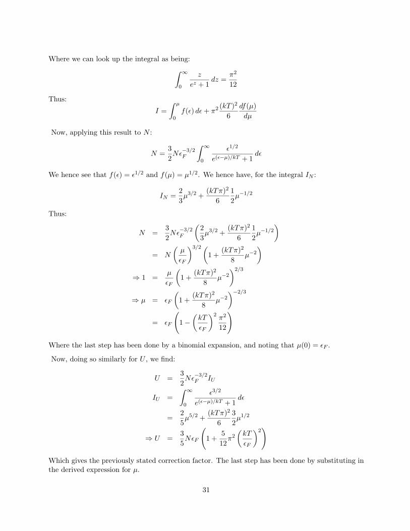
Where we can look up the integral as being:∫ ∞0

z

ez + 1dz =

π2

12

Thus:

I =∫ µ

0f(ε) dε+ π2 (kT )2

6df(µ)dµ

Now, applying this result to N :

N =32Nε−3/2F

∫ ∞0

ε1/2

e(ε−µ)/kT + 1dε

We hence see that f(ε) = ε1/2 and f(µ) = µ1/2. We hence have, for the integral IN :

IN =23µ3/2 +

(kTπ)2

612µ−1/2

Thus:

N =32Nε−3/2F

(23µ3/2 +

(kTπ)2

612µ−1/2

)= N

(µ

εF

)3/2(1 +

(kTπ)2

8µ−2

)⇒ 1 =

µ

εF

(1 +

(kTπ)2

8µ−2

)2/3

⇒ µ = εF

(1 +

(kTπ)2

8µ−2

)−2/3

= εF

(1−

(kT

εF

)2 π2

12

)

Where the last step has been done by a binomial expansion, and noting that µ(0) = εF .

Now, doing so similarly for U , we find:

U =32Nε−3/2F IU

IU =∫ ∞

0

ε3/2

e(ε−µ)/kT + 1dε

=25µ5/2 +

(kTπ)2

632µ1/2

⇒ U =35NεF

(1 +

512π2

(kT

εF

)2)

Which gives the previously stated correction factor. The last step has been done by substituting inthe derived expression for µ.

31

6.3 Example: Electrons in Metals

Now, if T < TF , we need to model electrons as behaving quantum mechanically.

For metals, we have data which show that TF ≈ 104 → 105K, and vF ≈ 1%c. Hence, metals atroom temperature behave via non-relativistic quantum mechanics.

If we suppose that the conduction electrons in a metal form a gas of free electrons, then it will be anon-relativistic degenerate fermi gas at room temperature. That is, occupancies of states below theFermi-energy is = 1. Now, electrons are actually (weakly) bound to the ionic lattice core, where thebinding will have the effect of dragging on the motion of electrons, and to thus increase the massof the electron, This effect will be ignored, but will be noted upon when we compare to data.

We have computed that quantum theory predicts:

Cquantumelectrons =π2

2NkB

(kBT

εF

)Where we have ignored any contributions to C due to the ionic core. So, what would classicaltheory predict? We have already done this, to the Einstein solid. It is just 1

2kBN per degree offreedom. Thus:

Cclasselectrons =32NkB

Now, if we include the contribution from the lattice 3NkB, where we have supposed 6 degrees offreedom (!):

Cclasstotal = 3NkB +32NkB =

92NkB

Now, experiment yields C ≈ 3NkB; which appears to be in agreement with the classical predictionwhere there are no electrons.

We can explain this discrepancy, by noting that Cquantumelectrons is small for T < TF . That is, if kBTεF << 1.Putting typical numbers in, we find that the quantum correction of the classical result is of the order1%. This would not show up on a crude experiment, but does in a more accurate experiment.

Heat capacities at low T have been accurately measured to go like:

C ≈ aT + bT 3

Where bT 3 is due to ionic contributions, and aT from electron contributions.

Experimental data results in a value for a:

a = 2.08× 10−3Jmol−1K−2

We get a value, from potassium data:

a =π2

2NkB

(kBεF

)= 1.7× 10−3Jmol−1K−2

So, our value is 20% off. This is however, our prediction with no ionic corrections. Our result shouldalways be smaller than experiment, as ionic cores ‘drag’ electrons back, effectively increasing theirmass.

a ∝ 1εF∝ m

32

Thus, if m were 20% bigger when ionic interactions taken into account, then the agreement wouldbe perfect.

6.4 Example: Liquid 3He

3He is a fermion.

Compute the Fermi-energy and find the temperature below which quantum effects are important.i.e. compute εF and TF . Given that the density is ρ = 81 kgm−3.Hence, we compute the number densirty n:

n =N

V=

813× 1.67× 10−27

= 1.6× 1028m−3

Where we have divided the density by the 3 times the mass of the proton. Hence, we have:

εF =h2

2m(3π2n)2/3 = 4.2× 10−4eV

TF =εFkB

= 5K

vF =

√2εFm

= 160ms−1

Where we have also compute the Fermi-velocity, to check that it is non-relativistic (which is blatantlyis!).So, for T < 5K, we expect:

CV =π2

2NkB

(kBT

εF

)= (1.0K−1)NkBT

And again, experiment yields 2.8K−1, which is higher than our prediction.Hence, interactions between 3He is obviously not negligible.

Especially at T < 2mK, where we have a discontinuity in the heat capacity at the transition intoa superfluid, where the 3He atoms pair up into bosonic pairs.

33

6.5 Example: Electrons in Stars

We start by asking: Do the electrons in the Sun form a degenerate fermi gas?

So, given that the core temperature is T ≈ 107K, we need to be able to compare it with the fermitemperature, which we need to calculate.Note, if T = 107K, then the thermal energy ε = kBT ≈ 107 × 10−23 ≈ 103eV. Now, this is a lothigher than the binding energy (= 13.6eV), hence there will not be much atomic hydrogen - it willbe mostly ionised. Now, we can compute TF via:

TF =kBεF

=1kB

h2

2m(3π2n)2/3

Where we have assumed non-relativistic.We can work out n via the mass of the Sun. If we assume that the Sun is only made up of protonsand electrons.

n =N

V=

M�Mp+Me

1V�

=M�Mp

1V�

Where we have used the fact that Me << Mp. We have also assumed one electron per proton.Using M� ≈ 2× 1030kg and R� ≈ 7× 108m, we have:

n ≈ 1030m−3

From which we can calculate:TF ≈ 105K

Which is two orders of magnitude less than the core temperature, therefore, T > TF , thereforeelectrons in the Sun do not form a degenerate fermi gas.

6.5.1 White Dwarf Stars

Stellar evolution starts with hydrogen gas collapsing under gravity to the point where pp fusion canoccur at T ≈ 107K. The stars radius is stabilised by the outward radiation pressure from the gas ofions, electrons and photons. The electrons are not (necessarily) degenerate. The outward radiationpressure is stabilised (or stabilises) the inward gravitational attraction due to mass.

When the proton fuel runs out, the radiation pressure falls, and the star collapses under gravityuntill the core becomes hot enough for the He to ignite at T ≈ 108K.

The process continues until no more nuclear fuel is left to burn. However, such stars are kept fromfurther collapse by the presence of an outward pressure due to the degenerate electron gas. Thesetypes of stars are called ‘white dwarfs’.

Now, given the mass of a white dwarf, we ought to be able to compute its radius.

Consider a shell at radius r, thickness dr. Now, the inward force due to gravity is balanced by theoutward force due to degenerate electrons. We can compute the inward gravitational force:

dF = 4πr2drρ(r)GM(r)r2

34

Where M(r) is the mass of the star inside a sphere is radius r. Notice that the volume of the shellis 4πr2dr, hence its mass is just 4πr2drρ(r).An outward force would come from a difference in pressure between the inner and outer surfaces ofthe shell, which would be of the form:

−dF = [p(r + dr)− p(r)]4πr2

= dp4πr2

Which we can substitute in for:

−dp4πr2 = 4πr2drρ(r)GM(r)r2

(6.12)

⇒ −dpdr

= ρ(r)GM(r)r2

(6.13)

⇒ −∫ p(R)

p(0)dp =

∫ R

0ρ(r)

GM(r)r2

dr (6.14)

Now, to do this integrals properly requires a numerical approximation. So we use various approxi-mations.We assume that p(0) >> p(R), thus helping with the integral on the LHS. We shall also assumethat any integral for the density ρ(r) over r results in some ‘average density’ ρ. Now, we have thatthe mass inside some sphere can be given by:

M(r) =∫ r

04πr2ρ(r′)dr′ = ρ

4πr3

3

Where we have used our approximation of average density. Thus, (6.14) becomes:

p(0) =∫ R

0ρ(r)

GM(r)r2

dr

= 4πGρ2

∫ R

0

1r2

r3

3dr

=4πGρ2R2

6≡ p

If we do the simple substitution that:

ρ =M

V=

M43πR

3

Then we have an expression for the inward pressure due to gravity:

p = 4πGR2

6

(M

43πR

3

)2

∝ M2

R4

Now, we have previously computed the pressure exerted by degenerate fermions:

p =25nεF =

25n5/3 h

2

2m(3π2)2/3

35

Where we can compute n as we did for the Sun. We assume the core to be composed of helium,which is 1 electron per proton. We use u to denote the atomic mass unit:

n =M

43πR

3

12u

Therefore, we have that the pressure due to the degenerate electrons is like:

p ∝ M5/3

R5

Thus, equating these two pressures (due to degeneracy and gravity) we obtain:

R = αM−1/3

α ≡ h2

2m32/3π4/3

(3

8πn

)5/3 8π3G

= 4× 1016mkg1/3

Data obtains α = 7 × 1016mkg1/3, which is a pretty good agreement! The agreement becomesabsolute if the density integral is done properly.

Hence, we see that such a star is stable, and degeneracy pressure ‘always’ wins. The reason forquotation marks, is that if the mass is above a certain limit, electron degeneracy pressure cannotsustain the equilibrium, and the star collapses further, into a neutron degenerate state.

We should check that the white dwarfs in the table are made of a degenerate core of electrons, andare not-relativistic.

We know that the temperature of the star T ≈ 107K. So, we need to compute TF .:

kBTF = εF =h2

2m(3π2n)2/3

To compute n, we do an order of magnitude calculation that is VERY rough:

n =M

u

143πr

3≈ 1030

10−271020≈ 1035m−3

Hence, we find that TF ≈ 109K > T . Hence, electrons degenerate.How fast are the electrons? We proceed via:

εF =12mv2

F = kBT

Hence, we have:

vF =

√2kBTm

= 107ms−1

Which is a lot less than c, hence non-relativistic.

What happens for more massive stars? We note that the electrons will become ultra-relativistic,and so we move from being able to use ε = h2k2

2m to having to use:

ε = hck

36

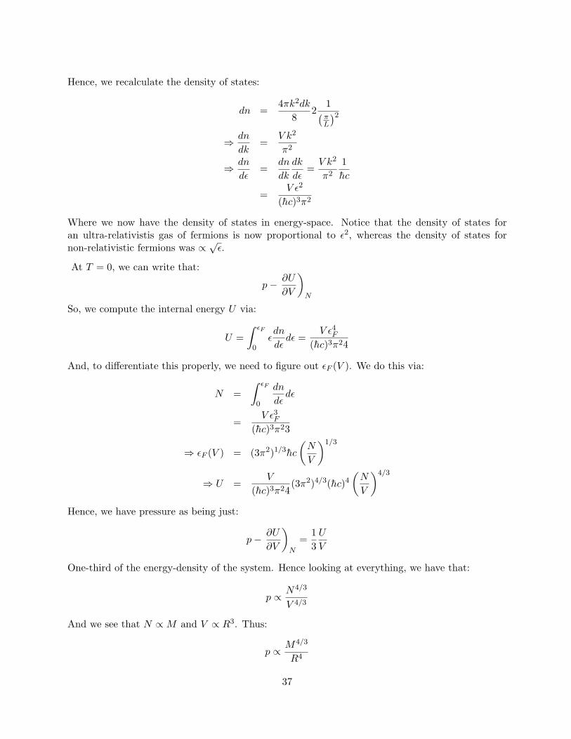
Hence, we recalculate the density of states:

dn =4πk2dk

82

1(πL

)2⇒ dn

dk=

V k2

π2

⇒ dn

dε=

dn

dk

dk

dε=V k2

π2

1hc

=V ε2

(hc)3π2

Where we now have the density of states in energy-space. Notice that the density of states foran ultra-relativistis gas of fermions is now proportional to ε2, whereas the density of states fornon-relativistic fermions was ∝

√ε.

At T = 0, we can write that:

p− ∂U

∂V

)N

So, we compute the internal energy U via:

U =∫ εF

0εdn

dεdε =

V ε4F(hc)3π24

And, to differentiate this properly, we need to figure out εF (V ). We do this via:

N =∫ εF

0

dn

dεdε

=V ε3F

(hc)3π23

⇒ εF (V ) = (3π2)1/3hc

(N

V

)1/3

⇒ U =V

(hc)3π24(3π2)4/3(hc)4

(N

V

)4/3

Hence, we have pressure as being just:

p− ∂U

∂V

)N

=13U

V

One-third of the energy-density of the system. Hence looking at everything, we have that:

p ∝ N4/3

V 4/3

And we see that N ∝M and V ∝ R3. Thus:

p ∝ M4/3

R4

37

For a gas of ultra-relativistic fermions.

Now, this dependance for the degeneracy pressure is such that there exists a maximum mass forwhich the pressures due to graviy and degeneracy balance. That is, there exists a maximum massfor which degeneracy pressure can sustain collapse due to gravity. This maximum mass is 1.4M�:the Chandrasekhar Mass.

As the star collapses εF rises. Eventually, particle physics becomes important and we get inversebeta-decay pe− → nνe and all protons and electrons dissapear leaving only neutrons; where theneutrinos will fly out. There will then be a neutron degeneracy pressure which supports againstfurther collapse (untill its critical mass of 1.8M� is reached).

7 Bose Gases

We are interested in low T behaviour. As T → 0 we expect even classically that particles willoccupy only the lowest energy level. So, how low must T be for macroscopic occupation of theground state? That is, the majority of particles in the ground state.

So, if we write down expressions for the two lowest possible energy states of a system:

ε0 =h2

2m

(πL

)2(12 + 12 + 12) ε1 =

h2

2m

(πL

)2(22 + 12 + 12)

Thus, the spacing between these levels is:

ε1 − ε0 =3h2

2m

(πL

)2

For the ground state to contain most of the particles, we want:

kBT ≤ ε1 − ε0

If L = 1cm, m = 6.6× 10−27kg, then:

T ≤ 10−681010−261−−4

= 10−14K

Which is very low! This however, has been calculated using classical arguments, and the result isvery different if we use a quantum mechanical description of identical particles.

Recall:〈n(ε)〉BE =

1e(ε−µ)/kBT − 1

Initially notice, when e(ε−µ)/kBT = 1 then the above becomes singular. We shall use the initialapproximation for the total number of particles:

N ≈∫ ∞

0

dn

dε

1e(ε−µ)/kBT − 1

dε

38

It will become clear as to why this is only an approximation. One thing to note is tha the densityof states is proportional to

√ε, and hence the result of this integral at the lowest single particle

energy state ε0 = 0 is zero. The exact form is actually purely a summation:

N =∑i

〈n(εi)〉

So, we start to analyse the distribution function:If N is fixed, then as T falls, µ must therefore rise. If we have that ε ≥ 0, and if we take theminimum energy level to be ε0, then we have µ ≤ ε0 so that there are no negative-particle-numberoccupancies (equivalent to saying there is always the requirement of ε−µ > 0) of any energy levels.We can set ε0 = 0, hence we have that µ ≤ 0.

Now, we see that there is a potential ‘problem’. µ cannot increase beyond ε0 = 0 at some criticaltemperature Tc. Hence, we have that µ = 0 at T = Tc. Thus, we can say (and this isnt anapproximation):

N ≡∫ ∞

0

dn

dε

1eε/kBTc − 1

dε

So, we have the interpretation that T = Tc is the lowest temperature in which 〈n〉BE works. Wesay this because for T < TC , we have that µ > 0, which is impossible.

So, lets compute 〈n〉BE for the lowest energy state ε0 = 0:

1e−µ/kBT − 1

=1

1− µkBT− 1

= −kBTµ≡ N0

Where we have use the Taylor expansion ex = 1 + x + x2 + . . .. Hence, we have that N0 is thenumber of particles in the ground state. Notice that N0 → ∞ as µ → 0. Now, we also know thatN0 ≤ N . Hence −kBT

µ ≤ N ; thus

µ ≥ −kBTN

Hence, as we have that µ ≤ 0 and the above ‘lower’ restraint, we have narrowed down the positionof µ very finely. For a system of 1023 particles, µ is very very close to zero, but not quite. In actualfact, the splitting between µ and ε0 is a lot less than that between ε0 and ε1.

We now have a new particle distribution function for T < Tc:

〈n〉 =1

eε/kBT − 1

Where we now have solved the problem of having µ > 0.

So, to summarise thus far, we have shown that as T → 0, the occupancy of the ground state, N0,tends to infinity. We also have that as T → 0, µ→ 0 very quickly for a macroscopic system.So, we can now write down a correct expression for the number of particle in the system: we takeout of the summation just the term due to the ground state:

N = N0 +∫ ∞

0

dn

dε

1eε/kBT − 1

dε

39

That we have not changed the lower limit of the integral is not a problem: the integral is zero forε = 0 anyway. Notice, we have also put µ = 0, as the energy level splitting is massive comparedto µ − ε0. Now, we can do this integral, after inserting in the expression for the density of statesin energy-space (for non-relativistic bosons). So, how does N0 vary for T < Tc, where we assumeµ = 0? So, writing the integral:

N = N0 +∫ ∞

0

V m3/2

√2π2h3

ε1/2 dε

eε/kBT − 1(7.1)

Now, we previously wrote that:

N ≡∫ ∞

0

dn

dε

1eε/kBTc − 1

dε

=V m3/2

√2π2h3

∫ ∞0

ε1/2 dε

eε/kBT − 1

=V m3/2

√2π2h3

(kBTc)3/2

∫ ∞0

(ε/kBTc)1/2 d(ε/kBTc)eε/kBT − 1

=V m3/2

√2π2h3

(kBTc)3/2

∫ ∞0

X1/2 dX

eX − 1

Infact, the integral can be looked up, to give:∫ ∞0

X1/2 dX

eX − 1= 2.315

Thus, (7.1) can be written:∫ ∞0

dn

dε

1eε/kBTc − 1

dε = N0 +∫ ∞

0

dn

dε

1eε/kBT − 1

dε

Now, we notice a similarlity between all factors in both integrals, except for T and Tc, which wecan factor out:

T 3/2c α = N0 + T 3/2α (7.2)

Where:

α ≡ V m3/2

√2π2h3

(kB)3/2

∫ ∞0

X1/2 dX

eX − 1

=N

T3/2c

Therefore, inserting this into (7.2) gives a relation for how the number of particles in the groundstate varies as T gets close to Tc:

N0 = N

[1−

(T

Tc

)3/2]

40

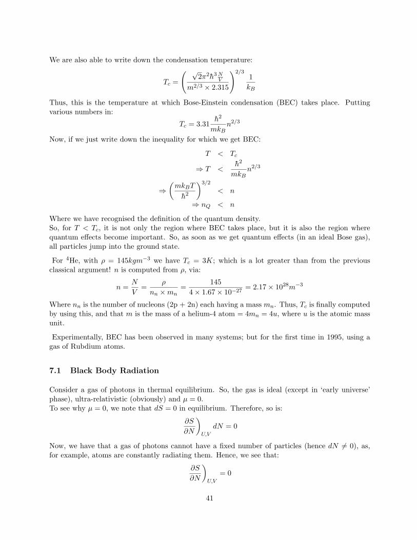
We are also able to write down the condensation temperature:

Tc =

( √2π2h3N

V

m2/3 × 2.315

)2/31kB

Thus, this is the temperature at which Bose-Einstein condensation (BEC) takes place. Puttingvarious numbers in:

Tc = 3.31h2

mkBn2/3

Now, if we just write down the inequality for which we get BEC:

T < Tc

⇒ T <h2

mkBn2/3

⇒(mkBT

h2

)3/2

< n

⇒ nQ < n

Where we have recognised the definition of the quantum density.So, for T < Tc, it is not only the region where BEC takes place, but it is also the region wherequantum effects become important. So, as soon as we get quantum effects (in an ideal Bose gas),all particles jump into the ground state.

For 4He, with ρ = 145kgm−3 we have Tc = 3K; which is a lot greater than from the previousclassical argument! n is computed from ρ, via:

n =N

V=

ρ

nn ×mn=

1454× 1.67× 10−27

= 2.17× 1028m−3

Where nn is the number of nucleons (2p + 2n) each having a mass mn. Thus, Tc is finally computedby using this, and that m is the mass of a helium-4 atom = 4mn = 4u, where u is the atomic massunit.

Experimentally, BEC has been observed in many systems; but for the first time in 1995, using agas of Rubdium atoms.

7.1 Black Body Radiation

Consider a gas of photons in thermal equilibrium. So, the gas is ideal (except in ‘early universe’phase), ultra-relativistic (obviously) and µ = 0.To see why µ = 0, we note that dS = 0 in equilibrium. Therefore, so is:

∂S

∂N

)U,V

dN = 0

Now, we have that a gas of photons cannot have a fixed number of particles (hence dN 6= 0), as,for example, atoms are constantly radiating them. Hence, we see that:

∂S

∂N

)U,V

= 0

41

However, we have the definition:

µ ≡ −T ∂S

∂N

)U,V

Therefore, we see that µ = 0. Hence, we have:

〈n(ε)〉 =1

eε/kBT − 1

Lets compute the energy density UV of a gas of photons:

U

V=

1V

∫ ∞0

dn

dε〈n(ε)〉ε dε

Using the ultra-relativistic form for the density of states in energy-space (previously derived) andusing a ‘spin multiplicity’ factor of 2, as there can be two polarisation states ‘in one’, we have:

U

V=

1V

∫ ∞0

V

π2

( εhc

)2 1hc

ε

eε/kBT − 1dε

=1

(hc)3π2

∫ ∞0

ε3

eε/kBT − 1dε

=(kBT )4

(hc)3π2

∫ ∞0

(ε/kBT )3

eε/kBT − 1d(ε/kBT )

=(kBT )4

(hc)3π2

∫ ∞0

X3

eX − 1dX

=(kBT )4

(hc)3π2

π4

15

⇒ U

V=

π2

15(hc)3(kBT )4

Now, to proceed, we shall discuss a little bit about blackbody radiation:Suppose we have a box of photons in thermal equilibrium (whose energy-density we have justcomputed). The box is completely isolated, except for a very small hole. Photons are able to leavethis hole, being in thermal equilibrium with the other photons still inside the box, hence blackbodyradiation. Any photons incident upon the hole, from outside, will be able to enter the hole, hencea blackbody absorber. If all photons inside the box move towards the side with the hole (of areaA), then the volume of photons being ejected per second is just cA. However, not all photons willbe moving in that direction, so we must integrate over the solid angle, to give 1

4cA.So, we ask the question, what is the power being radiated by the hole? This is just the total energyejected per second:

P =14cAU

VHence, inserting our expression for the energy density:

P =(

π2

60h3c2k4B

)T 4 ≡ σT 4

Where we have arrived at Stefan’s law, with his constant:

σ ≡ 5.67× 10−8Wm−2s−1K−4

Now, how is this power distributed over wavelengths? This will lead us to the Planck distribtion,and being able to predict the CMB.

42

Aside: CMB. The Cosmic Microwave Background arose in the very early universe. When thetemperature of the universe was so high that protons and electrons could not combine to formhydrogen, or any other elements, the ambient photons were being constantly scattered by this hot-plasma. As the universe cooled, Hydrogen formed, and photons stopped being scattered by theprotons and electrons. They had, however, been in thermal equilibrium with them. So, at the timeof recombination (where hydrogen formed), the photons suddenly had nothing to scatter off, so theymaintained their temperature/energy from when they were in thermal equilibrium. We are able tomeasure this background radiation.The CMB is a perfect blackbody radiation distribution, at a temperature of ≈2.7K. On a finerresolution however (order mK), we find anisotropies in the otherwise perfect blackbody spectrum.These anisotropies give information about how the very first matter was formed, in its density. Initaldensity fluctuations from recombination have left their mark in the form of the CMB anisotropies,and from this, we can find information about the early universe.

7.2 Spectral Energy Density

Now, lets calculate how the energy density UV is distributed over wavelengths λ. That is, the spectral

energy density.Now, we have that:

u(λ)dλ

Is the energy per unit volume, in the wavelength interval λ→ λ+dλ. Now, we previously calculatedthe total energy density:

U

V=

1π2(hc)3

∫ ∞0

ε3

eε/kBT − 1dε (7.3)

This is obviously the same as integrating u(λ)dλ over all λ. Hence:

U

V=

∫ ∞0

u(λ)dλ (7.4)

=1

π2(hc)3

∫ ∞0

ε3

eε/kBT − 1dε (7.5)

That is to say:

u(λ)dλ = 2dn

dεε〈n〉 1

Vdε

Where the factor 2 comes from there being 2 polarisation states.Now, we can find u(λ) by changing variables. We have that ε = hω = hc

λ . Thus:

dε = −hcλ2dλ

Thus, inserting these expressions into (7.3) results in:

U

V=∫ ∞

0

(hcλ

)3ehc/λkBT − 1

1π2(hc)3

hc

λ2dλ

43

Where the minus sign has been absorbed into the integrand, by symmetry arguments. If this is nowcompared with (7.4), we find (after cleaning up the above):

u(λ) =(2π)3hc

π2λ5

1ehc/λkBT − 1

Thus, we have derived what the energy density of a particular wavelength is: u(λ). This is knownas the Planck Formula. If we let λ → ∞, then we can Taylor expand the exponential, and we willend up with the classical Rayleigh-Jeans limit:

u(λ) = 8πhc

λ5

λkBT

hc=

8πkBTλ4

Notice, for this formula now (which is purely classical) there is a huge problem, and it is predictedthat u(λ = 0) = ∞. So, an infinite distribution for zero wavelength. This is, of course ridiculous,and is known as the UV-catastrophe.

We can find the wavelength which has maximum power associated with it. That is, a turning pointof the u(λ) curve. This is:

du

dλ= 0

This is known as Wein’s displacement law. However, to actually differentiate u(λ) gets tedious, sowe apply a ‘trick’. Let:

u ≡ f(x)λ5

x ≡ λT

Hence, if we write:

du

dλ=

d

dλ

(f(x)λ5

)=

1λ5

df

dλ+ f(x)

d

dλ

1λ5

=1λ5

df

dx

dx

dλ− f(x)

5λ6

=1λ5

df

dxT − f(x)

5λ6

= 0

⇒ 1λ5

df

dxT = f(x)

5λ6

⇒ xdf

dx= 5f(x)

Hence, the solution to this equation is that x =constant, or Tλ =constant.

Therefore, we have derived that the wavelength which has maximum power ascribed to it, at aparticular temperature, can be found from Tλ =constant. Thus, for two temperatures T1, T2; theirmaximum powers are at wavelengths λ1, λ2. If T1 < T2, then λ1 > λ2.

Sometimes we want u(ω)dω, which is the spectral distribution in terms of angular frequency.We have that ε = hω; and thus:

u(ω)dω = 2dn

dωdω〈n(ω)〉 hω

V

44

So, it remains to calculate the density of states in ω−space:

dn

dω=dn

dk

dk

dω

Using the relation ω = ck, we can then write:

dn

dω=

dn

dk

1c

=V k2

2π2

1c

=V ω2

2c2π2c

=V ω2

2c3π2

Therefore, putting everything in:

u(ω)dω = 2V ω2

2c3π2dω

1ehω/kBT − 1

hω

V

Cleaning up:

u(ω)dω =hω3

c3π2(ehω/kBT − 1)dω

Now, let us leave that alone.

7.2.1 Pressure of a Photon Gas

Let us now calculate the pressure due to a bose (photon) gas, in thermal equilibrium. To do so, wecalculate S, and differentiate it to get p. Recall that we have previously derived:

S = −kB∑states

e(µNs−Es)/kBT

Z

(µNs − EskBT

− lnZ)

Where the sum is over all single particle energy states. We have also derived:

lnZ = −∑i

ln(

1− e(µ−εi)/kBT)

Now, we have that µ = 0. We hence see that the expression for S simplifies somewhat:

S = −kB∑states

e−Es/kBT

Z

(−EskBT

− lnZ)

Notice that the first term is the same as writing∑

i piEi, which is just U . The second term is just:

kB lnZ∑i

pi = kB lnZ

45

The expression for lnZ can be made continuous via:

lnZ = −∫ ∞

0dεdn

dεln(1− e−ε/kBT )

Which we evaluate:

lnZ = − Vπ2

1(hc)2

∫ ∞0

ε2 ln(1− e−ε/kBT )dε

= − Vπ2

1(hc)3

(kBT )3

∫ ∞0

(ε

kBT

)2

ln(1− eε/kBT )d(

ε

kBT

)= − V

π2

1(hc)3

(kBT )3

∫ ∞0

X2 ln(1− e−X)dX

The integral is evaluated to give:∫ ∞0

X2 ln(1− e−X)dX = −13π4

15

Therefore, we see that:

S = −kB∑states

e−Es/kBT

Z

(−EskBT

− lnZ)

=kBU

kBT+ kB lnZ

=U

T+ V

(kBT

hc

)3 π2kB45

Now, we have previously derived that:

U

V=π2k4

BT4

15(hc)3

Hence, inserting things, and clearing up, results in:

S =U

T+

13U

T=

43U

T

Now the, pressure is found from:

p = T∂S

∂V

)U

Now, to do this properly, we need to be carefull; and find S(U, V ). Now, we just worked out (puttingall constants together):

U = aV T 4

46

Thus, we see that S = 43aV T

3. Therefore:

S =43aV

(U

aV

)3/4

=43a

(U

a

)3/4

V 1/4

⇒ ∂S

∂V

)U

=13a

(U

a

)3/4

V −3/4

=13a

(U

aV

)3/4

=13aT 3

⇒ p = T∂S

∂V

)U

=13aT 4

=13U

V

Hence, we have that the pressure exerted by a gas of photons is one third of the energy-density of thephotons. Which is, incidentally, an identical result as found for the pressure due to ultra-relativisticelectrons (fermions)

Now, for adiabatic expansions, we have that dS = 0. Classically, this corresponded with the resultof PV γ =const. However, here, if we look at the expression for S, and put it equal to a constant,we have:

V T 3 = const

For a photon gas.

8 Lattice Vibrations of a Solid

We’ve thus far been discussing a gas of photons by specifying the occupancies of each energy level.Thus, systems previously were determined by the set {ni}; where ni was the number of photons inenergy level εi. Thus, we were able to compute the average internal energy of the system via:

U =∑i

〈n〉iεi ≈∫ ∞

0

dn

dω〈n〉ε dω

We use this framework as an exact analogy to lattic vibrations of a solid:

Photons in energy level εi = hωi can be viewed as quanta associated with a set of quantum harmonicoscillators. That is, we model a solid as being a set of harmonic oscillators, each loaded with somequanta. The analogy goes that the set of harmonic oscillators is the same as the set of energy levelsof a photon gas. In quantising the lattic vibrations, we introduce the term ‘phonon’ as the analogyto ‘photon’ for a photon gas. A phonon is the quanta of lattice vibrations. A phonon is the sound

47

‘particle’, where a photon was a light ‘particle’.For a cube of some solid, with N atoms on some periodic lattice, there will be 3N normal modes.This is the total number of frequencies the system is allowed to vibrate in; such is the definition ofa normal mode.

So, we have that we have ni phonons in energy level εi. Hence, we have an energy nihωi onoscillator i. As we had no need (or idea) about a fixed number of photons in a system, we also havethat the number of phonons in a system is not fixed; thus, µ = 0 for lattice vibrations. We also useBose-Einstein statistics.

In Einstein’s model of a solid that we discussed at the start of the course, it was assumed that all3N oscillate with the same frequency; thus ε1 = ε2 = . . . = ε3N . So, for an Einstein solid:

UE =3N∑i=1

〈ni〉BEεi

=3N∑i=1

1ehω/kBT − 1

hωi

=3Nhω

ehω/kBT − 1

Which is a result that previously took us a lot longer to derive, as we previously had to physicallycount all states available. From this, we can just take the differential w.r.t. T to find the heatcapacity.

Now, Debye realised that the 3N modes do not oscillate with a single frequency - as Einstein hadassumed. But rather, the allowed frequencies are those of harmonic waves in a box. Thus, we havea wavenumber ki = niπ

L . Thus, we are able to write down a density of states. We use the relationk = ω

u , where u is the speed of wave propogation, which is the speed of phonons, which is the speedof sound. Thus:

dn

dω=

dn

dk

dk

dω

=V k2

2π2

1u

=V ω2

2π2u3

Now, the multiplicity factor we use is ‘3’. This comes from the consideration that we are able toexcite 2 transverse and 1 longitudinal sound waves in a 3d cube. Thus, the useable density of statesis thus:

dn

dω= 3

V ω2

2π2u3

So now, lets calculate the average energy of a Debye solid:

UD =∫ ωD

0

dn

dω〈n〉ε dω

Now, notice: for a photon gas, the upper limit was infinity. That was because there was an(essentially) infinite range of frequencies open to the system. We cannot assume this for latticevibrations. So, we assume that only ω < ωD, that is λ > λD. So, lets try to compute this cut-off.

48

Suppose atoms are spaced by an amount d. Then, the shortest possible wavelength that is able tobe fully supported by atoms are λD ≈ 2d. If we try to stick more than one wave between atoms,then nothing is excited, as there are no atoms there, hence pointless. Therefore, we are able toestimate the shortest wavelength that will be excited. The atomic spacing d is of the order 1

n1/3 , theinverse of the cube-root of the number-density. We see that ω is of the order u

λ (up to 2π). Hence:

ωD ≈ u(N

V

)1/3

We can calculate this exactly, by noting that there should be exacly 3N energy levels. So:

3N =∫ ∞

0

dn

dωdω

=3V

2π2u3

ω3D

3

⇒ ωD = u

(6π2N

V

)1/3

Therefore, we have an expression for the Debye cut-off frequency ωD. Notice, its in good agreementwith previous estimation. So, going back to the calculation of the internal energy of a Debye solid,inserting expressions for the density of states and BE distribution:

UD =3V h

2π2u3

∫ ∞0

ω3 dω

ehω/kBT − 1

This integral is hard to do, and we are unable to express it in the dimensionless terms we have usedfor bose gases. So, lets compute the heat capacity directly:

CD =∂U

∂T

=3V h

2π2u3

∫ ωD

0

ω3ehω/kBT

(ehω/kBT − 1)2

hω

kBT 2dω

Now, put:

x ≡ hω

kBT

Then:

CD =3V h

2π2u3

(kBT )4

h

1T

∫ xD

0

x4

(ex − 1)2dx

This can be cleaned up, after a lot of work, to:

CD = 3NkB

(3x3D

∫ xD

0

x4ex

(ex − 1)2dx

)Let us now look at the high and low temperature limits:

For high T , we see that x is small. Hence, the exponential in the bottom is expanded to ex = 1+x;and the exponential in the top just to unity. Thus, the integral itself is:∫ xD

0

x4

(x+ 1− 1)2dx =

∫ xD

0

x4

x2dx =

13x3D

49

Hence, we see:

CD ≈ 3NkB3x3D

x3D

3= 3NkB

Therefore, the high temperature behaviour of the heat capacity is a constant: CD = 3NkB.

In low temperatures, we see that x → ∞. Hence, the upper limit of the integral goes to infinity.We see that the ex

(ex−)2 term goes to e−x, for large x. Therefore, the integral just becomes:∫ ∞0

x4e−xdx

Which is just a number, β, say. Then:

CD ≈ 3NkB3x3D

β ∝ T 3

Hence, we see that the low temperature heat capacity goes as T 3. We find that experimental data

Figure 2: Heat capacity predictions of Debye and Einstein, Data will sit on Debye’s curve, asopposed to Einstein’s.

sits on the Debye curve, as opposed to that predicted with Einstein’s approximation.

50

A Colloquial Summary

This is a summary, based on the summary lecture.

The fundamental assumption pretty much everything is based upon is that for a closed system inequilibrium, all microstates are equally likely. Now, if a particular macrostate has more microstatesthan others, the it is more likely to be ‘picked’.There may be more than one way (microstate) of finding the system with a particular number ofparticles, energy, volume. These macroscopic quantities (N,U, V ) then define a macrostate.

A unique equilibrium macrostate usually exists. It is the macrostate with the overwhelmingly mostmicrostates. Now, we define entropy via S = −kB ln g. Where g is the number of microstates ina given macrostate. So, in equilibrium, S is a maximum. Thus, dS = 0. Therefore, for somemacroscopic variable X, ∂S

∂X = 0. This is a consequence of the chain rule. These variables are thenused to define temperature, chemical potential and pressure:

∂S

∂N∝ µ ∂S

∂U∝ T ∂S

∂V∝ p

Now, lets consider an ‘open system’; one that can transfer particles and energy with a reservoir. Wedo this by considering our system of interest as being part of a bigger system. Suppose our systemof interest has particle number and energy Ns, Us. Then, we have derived that the probability tofind the system in such a state; in a single quantum state (microstate) is:

P (Ns, Us) =eNsµ−UskBT

ZWhich is the Gibbs distribution.

From now, we shall consider our systems to be composed of non-interacting particles. We considerfermions and bosons. We can derive that the mean number of particles in a given quantum state is:

〈n〉FD =1

e(ε−µ)/kBT + 1

〈n〉BE =1

e(ε−µ)/kBT − 1

These tell us what the average number of particles in a particular energy state is.

We have the classical limit where 〈n〉FD ≈ 〈n〉BE ≈ eµ−εkBT . The classical limit can be interpreted

as being where the box defined by the de Broglie wavelength of the particles is very much less thanthe distance between the particles. Or, n << nQ, where nQ ≈ 1

λ3Q

.

We write some general formulae for finding the particle number N , internal energy U of the systemand entropy S:

N =∫ ∞

0

dn

dk〈n〉dk

U =∫ ∞

0

dn

dk〈n〉εdk

S = −kB∑

pi ln pi

I

The integral for N can be done, and then solved for the chemical potential µ. We must specifywhether to use non-relativistic or ultra-relativistic expressions ε = h2k2

2m or ε = hck. We now considerfermions and boson separately.

Fermions Fermions have anti-symmetric wavefunctions, which has the consequence of excludingthere ever being more than one fermion in a single particle energy state.We have considered examples of electrons in metals and white dwarf stars.We can use an approximation of T = 0 to rewrite the particle distribution function. We say thatthe occupancy of all (almost) single particle states below some ε = εF is total, and that (almost)no particles have energies above εF . Hence, the integral for the number of particles N has upperlimit kF , and 〈n〉 = 1 in this range. From this, we are able to derive an equation for εF , kF and useεF = kBTF to find the fermi-temperature.For T 6= 0, we imagine the step function crumbling over, to give the actual distribution. We usethis idea in calculating low temperature corrections to U . We say that the particles within kBT ofεF move up in energy by amount kBT . This allows us to write:

∆U =kBT

εFNkBT

That the internal energy is now dependent upon T gives the experimentally verified result of linearheat capacity. Note, at T = 0, U is independant of T , and C = 0.

Bosons Bosons have symmetric wavefunctions, and hence have no restriction on the number inany single particle energy state.We see that if N is fixed, then, as T falls, µ rises. We see that µ < 0; however, if T keeps decreasing,µ will go above zero (where zero is defined as being the same as the lowest energy state). Whenthis happens, there is a negative particle occupancy. So, to get around this, we say that below somecritical temperature, Tc, µ = 0. We say that Tc is the minimum temperature for which we canignore the ground state occupation. We also find that the ground state is macroscopically occupiedby particles. Infact, we define:

N ≡∫ ∞

0

dn

dε

1eε/kBTc − 1

dε

Now, for T < Tc, we are able to say that N = N0 +Ne, where N0 is the number in the ground stateand Ne is the number of particles in excited state, where:

Ne =∫ ∞

0

dn

dε

1eε/kBT − 1

dε

Using these two integrals, we are able to calculate the number of particle in the ground state. Weare also able to calculate Tc.

If we have a gas of photons in thermal equilibrium, we cannot expect the particle number to stayconstant; however, we still say that µ = 0, from considerations of the entropy in equilibrium. Thismodifies the BE distribution, to give us that for a gas of photons. We are easily able to computethe energy density of such a gas, and hence the power outputted per unit area, and can thus deriveStefan’s law P = σT 4. The distribution of this power over wavelengths (spectral distribution) can

II

thus be calculated. We write u(λ)dλ as being the energy per unit volume in a wavelength interval.We can write the same thing in ω:

u(ω)dω =1V

∫dn

dω〈n〉ε dω

Where we write ε = hω and the particle distribution is the modified BE distribution with µ = 0.Now, we actually have that:

U

V=∫u(ω)dω

As energy density. We are able to calculate the pressure exherted by a photon gas as being 13UV ,

which is the same as that due to ultra-relativistic electrons.

III

B Calculating the Density of States

The number of states dn, of spinless particles in a small 3D annulus, in k-space is given by thevolume of the annulus (which is 1

8 of the volume of the whole annulus) divided by the volume takenup by one state. Thus:

dn =184πk2dk(

πL

)3=

V k2

2π2dk

We have used that L3 = V . Hence, rearranging, we have the density of states, in k-space, of spinlessparticles:

dn

dk=V k2

2π2(B.1)

This will be our starting point for all subsequent calculations. To get the density of states in energy-space, we require a relationship between the wavenumber k and energy ε, and hence we must specifywhether or not the gas is non-relativistic, or ultra-relativistic (massless).

If the particles are fermions, and carry an intrinsic spin s, then this is modified to:

dn

dk= (2s+ 1)

V k2

2π2

If the particles are photons, they carry a spin of 1. However, we actually use a factor of 2, as thereare two polarisation states of a photon associated with each ‘state’. Hence, for photons:

dn

dk=V k2

π2

Proceeding with all subsequent calculations assume spinless.

B.1 Energy Space: Non-Relativistic

Suppose we want the density of states in energy space, that is:

dn

dε

We use the chain rule of differentiation to write:

dn

dε=dn

dk

dk

dε

The link between wavenumber k and energy ε, for non-relativistic particles is:

ε =h2k2

2m(B.2)

IV

Hence, rearranging:

k =(

2mh2

)1/2√ε

Therefore:dk

dε=(

2mh2

)1/2 12√ε

Now, we must also put dndk in terms of ε, which must be done using the non-relativistic expression

above in (B.2):dn

dk=V k2

2π2=

V

2π2

2mεh2

Therfore, putting this all together:

dn

dε=

dn

dk

dk

dε

=V

2π2

2mεh2

(2mh2

)1/2 12√ε

=V

4π2

(2mh2

)3/2√ε

So, the density of states, in energy-space, of a gas of non-relativistic particles is thus:

dn

dε=

V

4π2

(2mh2

)3/2√ε (B.3)

B.2 Energy Space: Ultra-Relativistic

If the gas is ultra-relativistic, we must use the following relation ε = pc, hence:

ε = hck (B.4)

Thus, we have the chain-rule expression:

dn

dε=dn

dk

dk

dε

Where we now see that:dk

dε=

1hc

We also have that:dn

dk=V k2

2π2=

V ε2

2π2(hc)2

Therefore, the density of states for an ultra-relativistic gas of spinless particles is:

dn

dε=

V ε2

2π2(hc)3(B.5)

V

C Deriving FD & BE Distributions

The Gibbs probability distribution:

P (N,U) =eβ(µN−U)

Z

Where β ≡ 1kBT

. That is, the probability to find the system with N particles and internal energyU .

Now, if we have an energy level εi, and ni particles occupying that level, then:

N =∑i

ni = n1 + n2 + n3 + . . .

U =∑i

niεi = n1ε1 + n2ε2 + n3ε3 + . . .

That is, ni is the number of ‘crosses’ on a particular energy level. Hence, Gibbs becomes:

P (N,U) =eβ(µ

Pi ni−

Pi niεi)

Z

=eβ

Pi ni(µ−εi)

ZThe Grand Partition Function Z is the sum for ni taking on all values (i.e. there being 1, 2, 3,. . . particles in energy level 1, and again for all other energy levels). That is:

Z =∑ni

eβPi ni(µ−εi)

=∑ni

eβ(n1µ−n1ε1)+β(n2µ−n2ε2)+β(n3µ−n3ε3)+...

=∑ni

∏i

eβ(niµ−niεi)

So, P (N,U) can be written:

P (N,U) =eβ

Pi ni(µ−εi)∑

ni

∏i eβ(niµ−niεi)

=∏i eβni(µ−εi)∑

ni

∏i eβ(niµ−niεi)

=eβn1(µ−ε1)eβn2(µ−ε2)eβn3(µ−ε3) . . .∑nieβn1(µ−ε1)eβn2(µ−ε2)eβn3(µ−ε3) . . .

=eβn1(µ−ε1)∑n1eβn1(µ−ε1)

eβn2(µ−ε2)∑n2eβn2(µ−ε2)

eβn3(µ−ε3)∑n3eβn3(µ−ε3)

. . .

= P (n1, ε1)P (n2, ε2)P (n3, ε3) . . .

So, the probability to find the system with N particles, and internal energy U is the product of theprobabilities of finding ni particles in energy level εi.

VI

So, the average number of particles in energy level εi is given by:

〈n(εi)〉 =∑

ni=0,1,2,...

P (ni, εi)ni

Where:

P (ni, εi) =eβni(µ−εi)∑nieβni(µ−εi)

Let us suppose that we only allow either 0 or 1 particles in each energy state (i.e. fermionic case);hence:

〈n(εi)〉 =∑ni=0,1

P (ni, εi)ni

= 0× P (0, εi) + 1× P (1, εi)

= 0× eβ0(µ−εi)∑n=0,1 e

βn(µ−εi)+ 1× eβ1(µ−εi)∑

n=0,1 eβn(µ−εi)

=eβ(µ−εi)

e0 + eβ(µ−εi)

=eβ(µ−εi)

1 + eβ(µ−εi)

=1

eβ(εi−µ) + 1

We have thus derived the Fermi-Dirac distribtion.Suppose that we allow any number of particles in each energy level; that is, ni can take on anynumber 0, . . . ,∞.

〈n(εi)〉 =∞∑ni=0

P (ni, εi)ni

=0 + e1β(µ−εi) + 2e2β(µ−εi) + . . .

1 + eβ(µ−εi) + e2β(µ−εi) + . . .

Here, we have noted that denominator (grand partition function) is actually a common factor to allexpressions. To evaluate this sum, we see that this is actually:

a+ 2a2 + 3a3 + . . .

1 + a+ a2 + a3 + . . .

Now, the sum∞∑i=0

ai =1

1− a,

is a standard result. We use this to find:

〈n(εi)〉 =1

eβ(ε−µ) − 1

We have thus derived the Bose-Einstein distribution.

VII