Thermal Hydraulic Analysis of a Reduced Scale High ...
228
THERMAL HYDRAULIC ANALYSIS OF A REDUCED SCALE HIGH TEMPERATURE GAS-COOLED REACTOR TEST FACILITY AND ITS PROTOTYPE WITH MELCOR A Thesis by BRADLEY AARON BEENY Submitted to the Office of Graduate Studies of Texas A&M University in partial fulfillment of the requirements for the degree of MASTER OF SCIENCE Approved by: Chair of Committee, Karen Vierow Committee Members, Pavel Tsvetkov Devesh Ranjan Head of Department, Yassin Hassan December 2012 Major Subject: Nuclear Engineering Copyright 2012 Bradley Aaron Beeny
Transcript of Thermal Hydraulic Analysis of a Reduced Scale High ...

THERMAL HYDRAULIC ANALYSIS OF A REDUCED SCALE
HIGH TEMPERATURE GAS-COOLED REACTOR TEST
FACILITY AND ITS PROTOTYPE WITH MELCOR
A Thesis
by
BRADLEY AARON BEENY
Submitted to the Office of Graduate Studies of Texas A&M University
in partial fulfillment of the requirements for the degree of
MASTER OF SCIENCE Approved by:
Chair of Committee, Karen Vierow Committee Members, Pavel Tsvetkov Devesh Ranjan Head of Department, Yassin Hassan
December 2012
Major Subject: Nuclear Engineering
Copyright 2012 Bradley Aaron Beeny

iii
ABSTRACT
Pursuant to the energy policy act of 2005, the High Temperature Gas-Cooled
Reactor (HTGR) has been selected as the Very High Temperature Reactor (VHTR) that
will become the Next Generation Nuclear Plant (NGNP). Although plans to build a
demonstration plant at Idaho National Laboratories (INL) are currently on hold, a
cooperative agreement on HTGR research between the U.S. Nuclear Regulatory
Commission (NRC) and several academic investigators remains in place.
One component of this agreement relates to validation of systems-level computer
code modeling capabilities in anticipation of the eventual need to perform HTGR
licensing analyses. Because the NRC has used MELCOR for LWR licensing in the past
and because MELCOR was recently updated to include gas-cooled reactor physics
models, MELCOR is among the system codes of interest in the cooperative agreement.
The impetus for this thesis was a code-to-experiment validation study wherein
MELCOR computer code predictions were to be benchmarked against experimental data
from a reduced-scale HTGR testing apparatus called the High Temperature Test Facility
(HTTF). For various reasons, HTTF data is not yet available from facility designers at
Oregon State University, and hence the scope of this thesis was narrowed to include only
computational studies of the HTTF and its prototype, General Atomics’ Modular High
Temperature Gas-Cooled Reactor (MHTGR). Using the most complete literature
references available for MHTGR design and using preliminary design information on the
HTTF, MELCOR input decks for both systems were developed. Normal and off-normal

iv
system operating conditions were modeled via implementation of appropriate boundary
and inititial conditions. MELCOR Predictions of system response for steady-state,
pressurized conduction cool-down (PCC), and depressurized conduction cool-down
(DCC) conditions were checked against nominal design parameters, physical intuition,
and some computational results available from previous RELAP5-3D analyses at INL.
All MELCOR input decks were successfully built and all scenarios were
successfully modeled under certain assumptions. Given that the HTTF input deck is
preliminary and was based on dated references, the results were altogether imperfect but
encouraging since no indications of as yet unknown deficiencies in MELCOR modeling
capability were observed. Researchers at TAMU are in a good position to revise the
MELCOR models upon receipt of new information and to move forward with
MELCOR-to-HTTF benchmarking when and if test data becomes available.

v
To my grandfathers, Billy Dye and Richard Beeny, who blessed my life by living theirs
as men of faith with a steadfast commitment to family

vi
ACKNOWLEDGMENTS
I would like to thank Dr. Karen Vierow for her guidance and support as my
employer, instructor, and faculty advisor ever since I began my time at TAMU in the fall
of 2006. Her confidence in me and expectations of me have served as useful motivation
during my undergraduate and graduate years. My association with her and the Nuclear
Heat Transfer Systems Labs has enriched my technical education and has lead to several
other professional relationships and developmental opportunities.
I would also like to thank the members of my thesis advisory committee: Dr.
Karen Vierow, Dr. Pavel Tsvetkov, and Dr. Devesh Ranjan. I very much appreciate their
time and technical advice. I have taken classes from each of them and know firsthand
their quality as educators and researchers.
Since my first technical internship at Sandia National Laboratories during the
summer of 2008, I have received much technical support from members of the reactor
modeling and analysis division with whom I worked. I would especially like to thank
Randy Gauntt and Larry Humphries for their several letters of recommendation in recent
years. I would also like to thank Mike Young and John Reynolds for their help.
Lastly, I wish to thank my family for the support they have never ceased to give
and for their unconditional love which I will never have to earn.

vii
NOMENCLATURE
ANS
American Nuclear Society
BISO
Bi-Isotropic
CF
Control Function
CL
Cladding Component
COR
Core Package
CV Control Volume
CVH
Control Volume Hydrodynamics Package
DCC
Depressurized Conduction Cool-Down
DCH
Decay Heat Package
DLOFC
Depressurized Loss of Forced Circulation
DOE
Department of Energy
EXEC
Executive Package
FL
Flow Path / Flow Path Package
FU
Fuel Component
GCR
Gas-Cooled Reactor
GTMHR
Gas Turbine Modular Helium Reactor
H2TS
Hierarchical Two-Tiered Scaling
HS
Heat Structure/ Heat Structure Package
HTGR
High Temperature Gas-Cooled Reactor

viii
HTR-10
High Temperature Reactor - 10
HTS
Heat Transport System
HTTF
High Temperature Test Facility
HTTR
High Temperature Test Reactor
INL
Idaho National Laboratories
LEU
Low Enriched Uranium
LWR
Light Water Reactor
MHTGR
Modular High Temperature Gas-Cooled Reactor
MP
Material Properties Package
NCG
Noncondensable Gas Package
NGNP
Next Generation Nuclear Plant
NRC
Nuclear Regulatory Commission
NS
Non-Supporting Structure Component
Nu
Nusselt Number
OSU
Oregon State University
PBMR
Pebble Bed Modular Reactor
PCC
Pressurized Conduction Cool-Down
PIRT
Phenomena Identification and Ranking Tables
PLOFC
Pressurized Loss of Forced Circulation
PMR
Prismatic Modular Reactor
Pr
Prandtl Number
PSER
Pre-Application Safety Evaluation Report

ix
PSID
Preliminary Safety Information Document
Ra
Rayleigh Number
RCCS
Reactor Cavity Cooling System
Re
Reynolds Number
RF
Reflector Component
SCS
Shutdown Cooling System
SNL
Sandia National Laboratories
SS
Support Structure Component
TAMU
Texas A&M University
TF
Tabular Function/ Tabular Functions Package
TRISO
Tri-Isotropic
VHTR
Very High Temperature Reactor

x
TABLE OF CONTENTS
Page
1. INTRODUCTION .......................................................................................................... 1
1.1 Thesis Objectives ............................................................................................. 2 1.2 Significance of Work ....................................................................................... 2 1.3 Technical Approach ......................................................................................... 3 1.4 Thesis Overview ............................................................................................... 4
2. MHTGR overview .......................................................................................................... 5
2.1 Brief History..................................................................................................... 5 2.2 Objectives ......................................................................................................... 6 2.3 General Design Description ............................................................................. 8
2.3.1 Fuel Design ....................................................................................... 8
2.3.2 Core Element Design ........................................................................ 9 2.3.3 Reactor Pressure Vessel, MHTGR Module, and Coolant Flow ...... 12 2.3.4 Reactivity Control Systems ............................................................. 13 2.3.5 Fuel Loading and Power Distribution ............................................. 14 2.3.6 Shutdown Cooling System and Reactor Cavity Cooling System ... 15
3. HTTF OVERVIEW ...................................................................................................... 19
3.1 Brief History................................................................................................... 19 3.2 Objectives ....................................................................................................... 20
3.3 General Design Description ........................................................................... 21
3.3.1 Core and Vessel Design .................................................................. 22 3.3.1.1 Typical Core Block Design .............................................. 23 3.3.1.2 Reflector Design ............................................................... 24
3.3.2 Reactor Cavity Cooling System Design .......................................... 25 4. MELCOR OVERVIEW ............................................................................................... 26
4.1 Background .................................................................................................... 26 4.2 Code Mechanics ............................................................................................. 27 4.3 Modeling Concepts ........................................................................................ 31
4.3.1 Control Volumes ............................................................................. 31 4.3.2 Flow Paths ....................................................................................... 35
4.3.3 Heat Structures ................................................................................ 36

xi
Page
4.3.4 Core Structures ................................................................................ 38 4.4 Gas-Cooled Reactor Physics .......................................................................... 42
4.4.1 Axial Conduction ............................................................................ 43 4.4.2 Radial Conduction ........................................................................... 44
4.4.2.1 General Inter-cell Conduction .......................................... 44 4.4.2.2 Tanaka-Chisaka Effective Conductivity .......................... 45 4.4.2.3 Intra-Cell Conduction and “Thick Cladding” .................. 46
4.4.2.4 Boundary Conduction ...................................................... 50 4.4.2.5 Convection ....................................................................... 51
5. MELCOR MODELING APPROACH AND INPUT DEVELOPMENT .................... 55
5.1 General MELCOR Modeling Approach ........................................................ 55 5.2 Specific MELCOR Modeling Approach ........................................................ 58
5.2.1 System Design Information ............................................................. 59 5.2.2 Core Nodalization ........................................................................... 59 5.2.3 Core Characterization ...................................................................... 64 5.2.4 In-Core Input ................................................................................... 69
5.2.5 Ex-Core Input .................................................................................. 71 5.2.6 Ancillary Input ................................................................................ 73 5.2.7 Steady-State and Transient Control Logic ...................................... 75 5.2.8 Decay Heat ...................................................................................... 77
6. RESULTS AND DISCUSSION .................................................................................. 78
6.1 Rationale for Test Case Selection .................................................................. 78 6.2 MELCOR Predictions .................................................................................... 79
6.2.1 MHTGR at 350 MWth ..................................................................... 79
6.2.1.1 Steady-State ...................................................................... 79 6.2.1.2 Pressurized Conduction Cool-Down ................................ 84 6.2.1.3 Depressurized Conduction Cool-Down ........................... 88
6.2.2 MHTGR at 35 MWth ....................................................................... 93 6.2.2.1 Steady-State ...................................................................... 93
6.2.2.2 Pressurized Conduction Cool-Down ................................ 97 6.2.2.3 Depressurized Conduction Cool-Down ......................... 100
6.2.3 HTTF at 2.2 MWth ......................................................................... 103 6.2.3.1 Steady-State .................................................................... 103 6.2.3.2 Depressurized Conduction Cool-Down ......................... 108
6.3 Prototype-to-Model Comparison with MELCOR Results ........................... 111
6.4 General Assessment of MELCOR/RELAP Agreement ............................... 113 7. CONCLUSIONS AND RECOMMENDATIONS ..................................................... 118

xii
Page
REFERENCES ............................................................................................................... 120
APPENDIX A: MHTGR INPUT/CALCULATION NOTEBOOK .............................. 122
APPENDIX B: HTTF INPUT/CALCULATION NOTEBOOK ................................... 165

xiii
LIST OF TABLES
TABLE Page
5. 1 Ceramic material properties for the MHTGR .................................................. 74
5. 2 Ceramic material properties for the HTTF ....................................................... 75 6.1 Steady-state parameters for the 350 MWth MHTGR……..…………………..80
6.2 Steady-state core structural temperature map for Figure 6.1 ........................... 81
6.3 Steady-state helium temperature map, 350 MWth MHTGR ............................ 84
6.4 Steady-state parameters for the 35 MWth MHTGR…………………………..93
6.5 Steady-state core structural temperature map for Figure 6.8 ........................... 95
6.6 Steady-state helium temperature map, 35 MWth MHTGR .............................. 97
6.7 Steady-state parameters for the 2.2 MWth HTTF……………………………104
6.8 Steady-state core structural temperature map for Figure 6.3 ......................... 105
6.9 Steady-state helium temperature map, HTTF ................................................ 107 A.1 Environmental variables input for MHTGR model ....................................... 122
A.2 EXEC MELGEN input for MHTGR model ................................................... 123
A.3 NCG input for MHTGR model ...................................................................... 123
A.4 CVH input for MHTGR model ...................................................................... 124
A.4.1 CV_NCG for MHTGR model ........................................................................ 125
A.4.2 CV_VAT for MHTGR model ........................................................................ 127
A.5 FL input for MHTGR model .......................................................................... 133

xiv
TABLE Page
A.5.1 FL_FT for MHTGR model ............................................................................. 134
A.5.2 FL geometric parameters for MHTGR model ................................................ 136
A.6 HS input for MHTGR model .......................................................................... 138
A.6.1 HS geometric parameters for MHTGR model ............................................... 139
A.6.2 HS LHS boundary conditions for MHTGR model ........................................ 141
A.6.3 HS RHS boundary conditions for MHTGR model ........................................ 142
A.7 COR input for MHTGR model ...................................................................... 143
A.7.1 COR_ZP for MHTGR model ......................................................................... 147
A.7.2 COR_RP for MHTGR model ......................................................................... 147
A.7.3 COR_RBV for MHTGR model ..................................................................... 148
A.7.4 COR_SS for MHTGR model ......................................................................... 149
A.7.5 COR_KFU for MHTGR model ...................................................................... 149
A.7.6 COR_KCL for MHTGR model ...................................................................... 149
A.7.7 COR_KSS for MHTGR model ...................................................................... 150
A.7.8 COR_KRF for MHTGR model ...................................................................... 151
A.7.9 COR_EDR for MHTGR model ...................................................................... 152
A.7.10 COR_RFD for MHTGR model ...................................................................... 152
A.7.11 COR_RFG for MHTGR model ...................................................................... 153
A.7.12 COR_BFA for MHTGR model ...................................................................... 154
A.7.13 COR_SA for MHTGR model ......................................................................... 156
A.7.14 COR_RFA for MHTGR model ...................................................................... 157

xv
TABLE Page
A.8 MP input for MHTGR model ......................................................................... 158
A.8.1 MP properties input for MHTGR model ........................................................ 159
A.9 TF input for MHTGR model .......................................................................... 160
A.9.1 TF tabular input for MHTGR model .............................................................. 160
A.10 CF input for MHTGR model .......................................................................... 163
A.10.1 CF arguments for MHTGR model ................................................................. 163
A.11 EXEC MELCOR input for MHTGR model ................................................... 164 B.1 Environmental variables input for HTTF model ............................................ 165
B.2 EXEC MELGEN input for HTTF model ....................................................... 166
B.3 NCG input for HTTF model ........................................................................... 166
B.4 CVH input for HTTF model ........................................................................... 167
B.4.1 CV_NCG for HTTF model ............................................................................. 168
B.4.2 CV_VAT for HTTF model ............................................................................. 171
B.5 FL input for HTTF model ............................................................................... 177
B.5.1 FL_FT for HTTF model ................................................................................. 178
B.5.2 FL geometric parameters for HTTF model .................................................... 180
B.6 HS input for HTTF model .............................................................................. 182
B.6.1 HS geometric parameters for HTTF model .................................................... 183
B.6.2 HS LHS boundary conditions for HTTF model ............................................. 186
B.6.3 HS RHS boundary conditions for HTTF model ............................................. 187
B.7 COR input for HTTF model ........................................................................... 189

xvi
TABLE Page
B.7.1 COR_SS for HTTF model .............................................................................. 193
B.7.2 COR_ZP for HTTF model .............................................................................. 193
B.7.3 COR_RP for HTTF model ............................................................................. 194
B.7.4 COR_RBV for HTTF model .......................................................................... 194
B.7.5 COR_KFU for HTTF model .......................................................................... 196
B.7.6 COR_KCL for HTTF model .......................................................................... 197
B.7.7 COR_KSS for HTTF model ........................................................................... 197
B.7.8 COR_KRF for HTTF model ........................................................................... 198
B.7.9 COR_RFD for HTTF model ........................................................................... 199
B.7.10 COR_RFG for HTTF model ........................................................................... 199
B.7.11 COR_BFA for HTTF model ........................................................................... 200
B.7.12 COR_SA for HTTF model ............................................................................. 202
B.7.13 COR_RFA for HTTF model ........................................................................... 204
B.8 MP input for HTTF model .............................................................................. 205
B.8.1 MP properties input for HTTF model ............................................................. 205
B.9 TF input for HTTF model ............................................................................... 206
B.9.1 TF tabular data for HTTF model .................................................................... 206
B.10 CF input for HTTF model .............................................................................. 207
B.10.1 CF arguments for HTTF model ...................................................................... 208
B. 11 EXEC MELCOR input for HTTF model ....................................................... 210

xvii
LIST OF FIGURES
FIGURE Page
2.1. TRISO fuel kernels, compacts, and elements .................................................. 9
2.2. Cross-sectional view of the MHTGR core .................................................... 11
2.3. MHTGR reactor vessel, cross duct, and secondary vessel ............................ 13
2.4. Shutdown cooling system loop ..................................................................... 15
2.5. Reactor cavity cooling system diagram ........................................................ 16
2.6. RCCS configuration, top view ...................................................................... 17 4.1. MELCOR execution flow diagram ............................................................... 27
4.2. Volume/altitude concept for control volumes ............................................... 33
4.3. Generalized COR nodalization ....................................................................... 39
4.4. COR package DT/DZ cell-wise energy balance concept .............................. 54 5.1. MELCOR input development flow diagram .................................................. 56
5.2. Geometric transformation of an HTGR core .................................................. 60
5.3. COR nodalization of the MHTGR ................................................................. 61
5.4. COR nodalization of the HTTF ...................................................................... 62
5.5. Channel and bypass flow area for an HTGR fuel element ............................. 66
5.6. Determination of an "effective clad radius" in an HTGR .............................. 68
5.7. Representative CVH nodalization for MHTGR/HTTF .................................. 72
5.8. DCH package decay heat curve based on ANS standard ............................... 77

xviii
FIGURE Page
6.1 Steady-state core structural temperature distribution ..................................... 82
6.2 Mass-averaged (by ring) core graphite temperatures during PCC ................. 85
6.3 Mass-averaged (by level) core graphite temperatures during PCC ................ 86
6.4 Area-averaged outer RPV wall temperature during PCC .............................. 88
6.5 Mass-averaged (by ring) core graphite temperatures during DCC ................ 89
6.6 Mass-averaged (by level) core graphite temperatures during DCC ............... 91
6.7 Area-averaged outer RPV wall temperature during DCC .............................. 92
6.8 Steady-state core structural temperature distribution ..................................... 96
6.9 Mass-averaged (by ring) core graphite temperatures during PCC ................. 98
6.10 Mass-averaged (by level) core graphite temperatures during PCC .............. 99
6.11 Area-averaged outer RPV wall temperature for PCC ................................ 100
6.12 Mass-averaged (by ring) core graphite temperatures during DCC ............ 101
6.13 Mass-averaged (by level) core graphite temperatures during DCC ........... 102
6.14 Area-averaged outer RPV wall temperature for DCC................................ 103
6.15 Steady-state core structural temperature distribution ................................. 106
6.16 Mass-averaged (by ring) core graphite temperatures during DCC ............ 108
6.17 Mass-averaged (by level) core graphite temperatures during DCC ........... 109
6.18 Area-averaged RPV outer wall temperature for DCC................................ 110
6.19 Ratio of structural temperatures in active core MHTGR-to-HTTF ........... 112
6.20 Hot-ring, mass-averaged FU temperature during PCC and DCC .............. 114
6.21 Peak fuel temperature as reported by RELAP during PCC and DCC [4] .. 115

xix
FIGURE Page
6.22 Area-averaged RPV outer wall temperature during PCC and DCC .......... 116
6.23 RPV temperature as reported by RELAP during PCC and DCC ............... 117

1
1. INTRODUCTION
The Department of Energy (DOE) has selected the high temperature gas-cooled
reactor (HTGR) as the Very High Temperature Reactor (VHTR) that will become the
Next Generation Nuclear Plant (NGNP) and will partially satisfy nuclear initiatives
calling for increased safety and reliability. Prior to the economic downturn of 2008,
plans were in place to build an NGNP demonstration plant at Idaho National
Laboratories (INL) as per the Energy Policy Act of 2005. Realization of this goal is
unlikely under present circumstances, but a cooperative agreement on HTGR research
remains in place between several academic institutions and the Nuclear Regulatory
Commission (NRC). The overall goal of the cooperative agreement is to expand the
HTGR knowledge base through integral facility experiments, separate effects tests, and
various computational studies. Texas A&M University (TAMU), as a party to this
agreement, was appointed several tasks related to HTGR analysis. The studies detailed
in this thesis follow from cooperative agreement research directives involving systems-
level HTGR predictive simulations and a code-to-experiment benchmark.
MELCOR is a systems-level thermal hydraulics and severe accident computer
code developed by Sandia National Laboratories (SNL) for the NRC. It has been used as
a safety analysis tool to license light water reactors (LWRs) but was recently modified
for application to HTGRs. Validation of its predictive capabilities is necessary to qualify
MELCOR as a reliable NRC licensing tool for future HTGR installations. Hence, the
need for a code-to-experiment benchmark study involving MELCOR is evident and was
to be addressed through construction of a High Temperature Test Facility (HTTF) at
Oregon State University (OSU). The HTTF is a reduced-scale model of General

2
Atomics’ Modular High Temperature Gas-Cooled Reactor (MHTGR), which was the
prototypical HTGR for the HTTF. Despite recent delays in construction and in
commencement of shake-down testing, the need may still arise in the near future for
validation of TAMU MELCOR models against the HTTF test matrix. The MELCOR
models explained in this thesis would facilitate a future MELCOR-to-HTTF benchmark
exercise, but only limited MELCOR validation activity is currently possible.
1.1 Thesis Objectives
The objectives of this thesis are as follows:
To develop MELCOR input decks for the reduced-scale High Temperature Test
Facility and its prototype, the Modular High Temperature Gas-Cooled Reactor
using the latest references
To apply and to test newly-implemented Gas-Cooled Reactor (GCR) MELCOR
models as they pertain to HTGR thermal hydraulics
To assess MELCOR capabilities for modeling normal (steady-state) and off-
normal (pressurized/depressurized conduction cool-downs) HTGR operating
scenarios by comparison with nominal design parameters and previously
published results of other computer codes
To make recommendations for improvements to MELCOR based on findings
To prepare for future HTTF code-to-experiment benchmark studies
1.2 Significance of Work
Recent concern about materials temperature limits has caused downward
revisions to the NGNP target outlet temperature. “High Temperature” or “Very High
Temperature” as in HTGR/VHTR generally refers to core outlet temperatures

3
approaching 1000 °C. This outlet temperature is attractive from a thermodynamic
perspective (increased thermal efficiency, less waste heat rejection) but also enables
energy/hydrogen co-generation (via high-temperature electrolysis) and lends itself to any
of several other industrial applications. The theoretically achievable outlet temperature
of an HTGR makes it an attractive alternative to an LWR, but the appeal lessens at lower
HTGR target outlet temperature. NGNP outlet temperature revisions have dropped the
target from 1000 °C to less than 700 °C. As a direct result, both the NGNP program
(supported by the DOE) and the cooperative agreement on HTGR research (supported
by the NRC) have received less support recently. However, one may still anticipate a
future need for HTGR licensing tool validation and it is in this sense that the work of this
thesis bears relevance to the nuclear industry and to its regulators.
1.3 Technical Approach
Pursuant to aforementioned thesis objectives, MELCOR input decks were built
for the MHTGR and the HTTF using the latest system design documents and the most
recent GCR physics modeling features of MELCOR. For the MHTGR, the primary
source of design information was a decades-old Preliminary Safety Information
Document (PSID) submitted to the NRC and designated as HTGR-86-024. For the
HTTF, the primary source of design information was the most recent set of design
drawings obtained through direct communication with facility designers at OSU. To a
lesser extent, the OSU report on HTTF scaling analysis also served as a useful reference.
After extensive debugging, the basic input decks were fine-tuned and control logic was
built in to allow for modeling of steady-state, pressurized conduction cool-down (PCC),
and depressurized conduction cool-down (DCC) scenarios. Several assumptions were

4
made at this stage of the process because there is considerable uncertainty associated
with off-normal HTGR operations. After gathering results, an attempt was made to
partially validate MELCOR predictions of core thermal hydraulic response by
comparison with nominal MHTGR/HTTF design parameters and published RELAP
code results from INL.
1.4 Thesis Overview
Chapters 2 and 3 present overviews of the MHTGR and the HTTF, respectively,
and include brief discussions of history, programmatic objectives, and design for each
system. Chapter 4 gives insight in to the MELCOR code by introducing general code
mechanics and modeling concepts before describing several relevant GCR physics
models. Chapter 5 outlines the MELCOR modeling approach taken for both the
MHTGR and the HTTF and goes on to describe the implementation of steady-state and
conduction cool-down cases via control logic and boundary conditions. Chapter 6
presents results for the various analyses from which the useful conclusions and
recommendations of chapter 7 are drawn. In the appendices, representative MELCOR
input decks in tabular form are included for reference.

5
2. MHTGR OVERVIEW
2.1 Brief History
In the mid-1980’s, the DOE submitted to the NRC the PSID for the MHTGR.
The nuclear power system described therein was meant to be a simple, safe, economic,
competitive alternative to LWRs for the nuclear power industry. In anticipation of the
eventual need for licensing, the NRC responded to the MHTGR PSID with a Pre-
application Safety Evaluation Report (PSER) designated as NUREG-1338 [5]. Various
other DOE reports regarding different special topics were also submitted to the NRC for
review around the same time. The nuclear system described by the DOE’s PSID of 1986
and the NRC’s NUREG-1338 of 1995 is the HTGR to which the HTTF is scaled.
Several countries have accrued substantial operating experience with gas cooled
reactors since the European (U.K. and France) Magnox reactors of the 1950’s.
Germany, Japan, and China have had operational GCRs (experimental and/or power
producing). With respect to HTGRs in the U.S., two facilities are of note for their
similarities to the MHTGR: Fort St. Vrain in Colorado and Peach Bottom-1 in
Pennsylvania. Unit 1 of the 40 MWe Peach Bottom Atomic Power Station operated from
the late 1960’s to the early 1970’s. It had a prismatic core, BISO-coated fuel particles,
helium coolant, and a prismatic core design. The 330 MWe Fort St. Vrain generating
station operated from 1976 to 1989 and used TRISO-coated fuel particles with a
prismatic core design. Lessons learned from the combined twenty years of HTGR
operating experience in the U.S. may be leveraged for licensing purposes. For example,
observations of fission product retention capability (at Fort St. Vrain) could help the

6
NRC to decide whether low-leakage LWR-style containment is a necessity for a TRISO-
fueled HTGR.
NRC documents summarizing domestic operational experience have been
published (e.g. NUREG-CR-6839 regarding Fort St. Vrain). A myriad of technical
documents and research reports on GCR phenomenology are also available for review.
Taken together, research efforts and operational experience world-wide have contributed
to a fairly robust GCR knowledge base. Still, HTGR operational experience is limited as
only Chinese and Japanese test reactors (HTR-10 and HTTR, respectively) are currently
or were recently online. Of those two facilities, only the HTTR bears any similarity to
the MHTGR. The state of the art of HTGR design has therefore had little chance to
evolve in response to lessons learned from operational experience (compared to the state
of the art in LWR design). Nevertheless, HTGRs have been proven viable and safe
through limited industrial activity.
2.2 Objectives
The MHTGR was designed to be a passively safe and economic alternative to
gen. II-III LWRs and was among the industry’s first answers to congress’ 1984 request
for a simpler, safer fission power system. By reducing reliance on both operator action
and active equipment, two factors often contributory to accident initiation/progression
are minimized in potential impact. If operator intervention is not required to mitigate an
accident, there is no chance that human error could exacerbate an event in progress. If
fewer mechanically-active components comprise a given system, there is a smaller
chance that mechanical failure may render it inoperable. Compared to an LWR, the
MHTGR reduces reliance on operator action during off-normal conditions and can

7
inherently mitigate/manage accidents via its passive safety features and design
characteristics. This “walk-away safety” of the MHTGR is its most attractive attribute.
High core material melting points, a low power density, and a high core/reflector
heat capacity generally lead to sluggish MHTGR thermal transients. Core overheating is
unlikely and could only occur if all cooling (including passive conduction/radiation) is
lost for an extended time. Aforementioned attributes of the MHTGR contribute in part
to satisfying the foremost objective of any nuclear power system, which is the
preservation of public/environmental health and safety. To that end, the MHTGR design
gives due consideration to siting criteria and standards for radiation protection as
outlined in the various codes of federal regulations.
The MHTGR, unlike the higher temperature Gas Turbine Modular Helium
Reactor (GTMHR), employs a Rankine power cycle for electricity production. The
target core outlet temperature (690˚C) is likely too low to be of use for
electricity/hydrogen co-generation via electrolysis. However, there exists a wide array
of potential industrial applications for MHTGR process heat or reduced pressure steam.
Of course, such possibilities give rise to certain licensing issues that do not exist for
LWRs. One might also imagine alternative MHTGR fuel cycles tailored for specific
purposes (e.g. transmuting reprocessed LWR transuranics in TRISO fuel), but such
applications were not among the HTGR primary programmatic objectives in the 1980’s.
More recently, generation IV initiatives have called for HTGR designs that can
both enhance proliferation resistance and reduce the domestic LWR spent fuel inventory.
The GTMHR more completely addresses gen. IV objectives than does the MHTGR and
offers more latitude in the way of process heat or co-generation applications. Because of

8
comparatively higher temperatures and coupled gas turbo-machinery (Brayton power
cycle), GTMHR thermal efficiency is higher than that of the MHTGR and allows for
reduced thermal pollution. Overall, the GTMHR satisfies all design objectives of the
MHTGR while simultaneously reducing environmental impact and heavy metal wastes
(relative to LWRs). Most research done at the MHTGR-based HTTF will bear some
relevance to the GTMHR because of the resemblance in core design.
2.3 General Design Description
The MHTGR is similar to other previously licensed HTGR facilities such as Fort
St. Vrain and Peach Bottom-1. However, DOE’s programmatic objectives for the
MHTGR necessitate certain safety and high-temperature design characteristics that
distinguish it from previous systems. Safety characteristics include a low power density,
a large and negative core Doppler coefficient of reactivity, a high heat capacity, a
chemically and neutronically inert single phase coolant, and passive decay heat removal.
These features prevent and mitigate (two pillars of defense-in-depth) potential accidents.
2.3.1 Fuel Design
The MHTGR is a thermal-spectrum reactor that uses tri-isotropic (TRISO)
coated fissile (uranium) and fertile (thorium) fuel kernels suspended in carbonaceous
cylindrical compacts (12.45 mm diameter, 49.3 mm long) that are stacked in hexagonal
graphite blocks (fuel elements). A cut-away view of a typical TRISO particle is included
in Figure 2.1 as are pictures of fuel compacts and elements.

9
Figure 2.1. TRISO fuel kernels, compacts, and elements [6]
Uranium-bearing fuel kernels are 19.9% enriched (by weight), just under the
20% LEU limit. The various layers of kernel coating ensure structural integrity and
fission product retention of each TRISO particle. The porous carbon buffer traps gaseous
fission products and absorbs recoil energy while the silicon carbide layer provides
structural stability against thermal and mechanical stresses. The outermost pyrolitic
carbon layer acts as yet another barrier to fission products. The cylindrical graphite
compacts maximize fuel conductivity and hinder fission product escape.
2.3.2 Core Element Design
The fuel elements are right hexagonal prisms (0.793m tall, 0.36m across flats)
stacked ten high in an annular arrangement around a central reflector region and inside a

10
peripheral reflector. Each has coolant and fuel holes and a few have reserve shutdown
control rod holes. Graphite regions are present above and below the active core for
additional neutron reflection. Ceramic structures above the flow distribution block in the
lower reflector are made of nuclear grade H451 graphite. Coolant channels and control
material holes are present as necessary in the upper reflector, the outer portion of the
central reflector, the inner portion of the side reflector, and the lower reflector. The
innermost elements of the central reflector and the outermost regions of the side reflector
are solid. MHTGR core layout is shown in Figure 2.2.
Hex blocks comprising the upper and lower reflectors are not all identical in
height. The top reflector consists of two layers: a top layer of full height (0.793m) and a
bottom layer of half height. The lower reflector consists of a three-quarters height layer
atop a half height layer that acts to distribute coolant flow to the lower plenum. For
purposes of construction, shuffling, and replacement, all blocks have handling holes at
their geometric centers. Sockets are carved out of each block to accommodate graphite
dowels that hold stacked structures together.

11
Figure 2.2. Cross-sectional view of the MHTGR core [6]
Several metallic components (Alloy 800H) designed for various purposes are
present around the graphite core. Lateral restraints and the metallic support structure
help to hold graphite in place. The upper plenum thermal protection structure shields the
metallic vessel from thermal loads and provides a sealed upper plenum region that
facilitates coolant flow. The metallic core barrel, up-comer ducts, and vessel wall all
play important roles in core cooling (under both normal and accident conditions) as does
the metallic cross duct leading to and from the reactor vessel. Also, metallic plenum
elements (alloy 800H) resting atop the upper reflector serve to limit core bypass flow
and provide neutron shielding for the rest of the upper plenum. Plenum elements differ
in form and function depending on their radial location above the upper reflector.
Elements on top of the active core region have all requisite coolant channels and reserve

12
shutdown control rod holes. Elements above the central or side reflector may or may not
have coolant holes. Plenum blocks contain borated graphite pellets for neutron shielding.
2.3.3 Reactor Pressure Vessel, MHTGR Module, and Coolant Flow
The MHTGR steam cycle plant module is pictured in Figure 2.3, with the reactor
vessel on the left and the steam generator vessel on the right. The nuclear island contains
four 350 MWth modules, each housed in an underground concrete silo that acts as a
vented containment. Nominally, the core power density is 5.9 MWth/m3 and the primary
loop is pressurized to about 6.4 MPa.
The two vessels in each module are connected by a concentric cross duct through
which hot helium exits the reactor vessel (through the inner channel) and cold helium
enters the reactor vessel (through the outer channel). From the cross duct, cold helium is
sent to up-comer ducts that lead to the upper plenum. Helium is then turned back
downwards to flow through the core before being collected and mixed in the lower
plenum. At core inlet conditions, the helium temperature is about 260 ˚C and is flowing
at 157 kg/s. It is estimated that about 11% of the coolant flow bypasses the active core
and is channeled through central reflector coolant holes, small control rod coolant
passages, and intervening gaps between graphite blocks. Helium passing through core
coolant channels sees no change in flow geometry across the core, leading to negligible
form losses and a relatively small friction pressure drop. Coolant experiences a transition
in channel geometry at the lower reflector flow distribution block just before it reaches
the lower plenum. On average, the coolant exit temperature is 690 ˚C, but localized “hot
streaks” could be significantly hotter.

13
Figure 2.3. MHTGR reactor vessel, cross duct, and secondary vessel [6]
2.3.4 Reactivity Control Systems
Burnable poisons, standard control rods, and reserve shutdown control rods
comprise the reactivity control strategy. Burnable poison (borated graphite pins) is
included at the hexagonal corners of each fuel element to cope with excess reactivity
over the course of core lifetime. Standard control rods reside in the central and side
reflectors and consist of 40 weight percent enriched boron carbide granules dispersed in
graphite rods that are canned in alloy 800H. Reserve shutdown control “pellets”

14
containing boron carbide are available for emergency insertion to reserve shutdown fuel
elements. Thus, there is no control material other than burnable poison in the active core
region under normal operating conditions. This design differs considerably from that of
LWR’s and is explained by the greater relative reactivity worth of control rods located in
regions of peak thermal neutron flux (reflectors) vs. control rods dispersed throughout
the active core.
Overall, reactivity temperature/power feedback is inherently negative under
conceivable operating conditions. Major contributing effects include prompt fuel
Doppler feedback, graphite moderator temperature feedback, and reflector temperature
feedback. The first two feedback effects are negative, while the last one is small and
positive for reasons related to control rod worth in reflectors subsequent to heat-up. By
design, the helium coolant is neutronically transparent regardless of temperature. The
delayed neutron fraction is approximately 0.0065 near the beginning of core life but
evolves as a function of the fissile nuclide inventory thereafter.
2.3.5 Fuel Loading and Power Distribution
The metal inventory of a fresh MHTGR core consists of approximately 2.346
metric tons of thorium and 1.726 metric tons of uranium, which allows for an initial
cycle length of just less than 2 years. The next three “transition reload” cycles call for
replacement of half the core every 1.5 years. The Equilibrium burn-up cycle is then
reached, where half the core is replaced every 1.65 years. Enrichment zoning is not part
of the axial or radial power shaping strategy, but zoning by average fissile/fertile
material concentration is employed to shift power radially outward. Axially, the profile
is top-peaked so that incoming coolant first encounters regions of highest power.
15
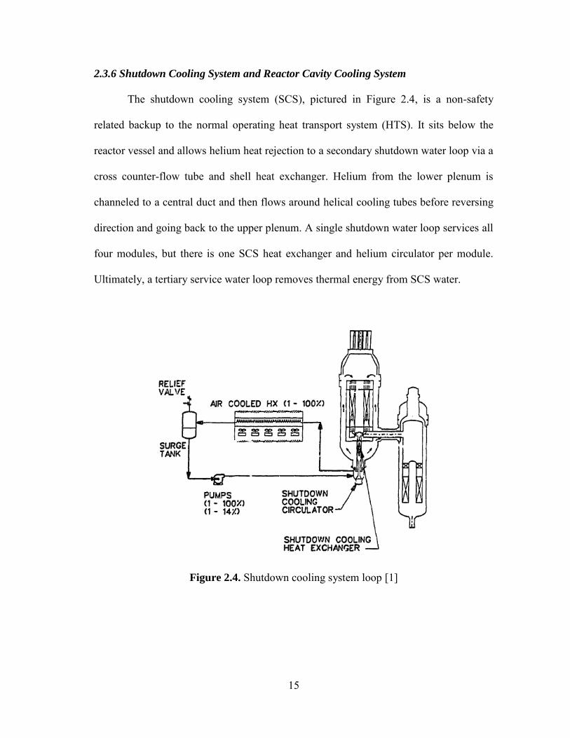
2.3.6 Shutdown Cooling System and Reactor Cavity Cooling System
The shutdown cooling system (SCS), pictured in Figure 2.4, is a non-safety
related backup to the normal operating heat transport system (HTS). It sits below the
reactor vessel and allows helium heat rejection to a secondary shutdown water loop via a
cross counter-flow tube and shell heat exchanger. Helium from the lower plenum is
channeled to a central duct and then flows around helical cooling tubes before reversing
direction and going back to the upper plenum. A single shutdown water loop services all
four modules, but there is one SCS heat exchanger and helium circulator per module.
Ultimately, a tertiary service water loop removes thermal energy from SCS water.
Figure 2.4. Shutdown cooling system loop [1]

16
The reactor cavity cooling system (RCCS) pictured in Figure 2.5 is the passive
safety-grade core cooling system that makes the MHTGR “walk-away safe”. It involves
no active components but instead relies on naturally-occurring phenomena to remove
residual heat from the reactor vessel to the environment. In the event the normal HTS or
SCS is unavailable, the RCCS automatically intervenes (without reliance on operators or
actuation signals of any kind) to cool the metal vessel wall. As designed, the RCCS is
air-cooled, but water-cooled alternatives have been proposed.
Figure 2.5. Reactor cavity cooling system diagram [1]

17
The RCCS consists of a cooling panel array that encloses the bare steel reactor
vessel wall. Cold down-comer passages and insulated hot riser ducts facilitate natural
draft air cooling. Across the intervening reactor cavity air space, the steel vessel surface
radiates thermal energy to the steel RCCS panels so that natural circulation can carry this
energy outside the system. Figure 2.6 below shows a top view of the pressure vessel
wall, reactor cavity, and RCCS panels.
Figure 2.6. RCCS configuration, top view [1]

18
It is expected that radiation accounts for roughly 90% of the vessel heat removal,
with the balance removed by cavity air circulation. Sufficient redundancy is built in to
each module’s RCCS, as there are hundreds of independent panels (hot ducts) and four
separate inlets/outlets to communicate with the environment. Provided the core
conduction pathway is not degraded, the RCCS can maintain core material temperatures
below damage limits and thereby preclude a significant radioactivity release.

19
3. HTTF OVERVIEW
3.1 Brief History
As part of a recent cooperative agreement on HTGR research between the NRC
and several academic researchers, Oregon State University was tasked with the design
and construction of an integral test facility for study of HTGR thermal hydraulic
phenomena. As the first of its kind in the U.S., it is envisioned that the HTTF will
furnish valuable thermal hydraulics data that better characterizes some potential
challenges of prismatic-type HTGR operation. Special attention will be afforded to “high
priority and low knowledge” issues identified in a recent DOE Phenomena Identification
and Ranking Table (PIRT) study (part of the NGNP project, 2008) [7]. For normal
operating conditions, these issues include helium hot streaking, bypass flow, and other
matters related to coolant flow distribution. For off-normal conditions, coolant behavior
and overall system response during pressurized and/or depressurized conduction cool-
down (P/DCC) is of great concern.
With the DCC event in mind, OSU performed a scaling analysis in accordance
with NRC severe accident scaling methodology as described in appendix D of
NUREG/CR-5809 [8]. Application of this Hierarchical Two-Tiered Scaling (H2TS)
method resulted in a conceptual HTTF design and helped to quantify scaling distortions
where similitude between prototype and model could not be preserved. It should be
noted that the scaling analysis was performed for HTGRs of both prismatic or pebble-
bed type. The MHTGR and/or the GTMHR are obvious references for prismatic-type
HTGRs, but no specific consideration was given to either design in the scaling analysis.

20
3.2 Objectives
Integral HTTF experiments will address several deficiencies in the present
knowledge base and will hopefully advance the state of the art of HTGR design. A
judicious instrumentation plan and a well-designed test matrix will enable code-to-
experiment benchmark studies with MELCOR (and other codes) to advance the state of
the art of reactor thermal hydraulic analysis. Expansion of the knowledge base and code
validation are of paramount importance to the NRC insofar as licensing, especially if the
existing NRC code suite (of which MELCOR is a part) will be utilized for HTGR design
basis and licensing calculations.
The NGNP PIRT [7] identified poorly understood physical phenomena
associated with pressurized/depressurized losses of forced circulation (P/DLOFC). These
events are also called pressurized/depressurized conduction cool-downs because after a
loss of forced circulation, the main core cooling modes are radial conduction and
radiation to the passive reactor cavity cooling system (RCCS) panels. In a pressurized
conduction cool-down, there is no break in the pressure boundary and reactor vessel
depressurization does not occur. The coolant will stagnate before eventual establishment
of natural circulation. In a depressurized conduction cool-down, helium coolant crosses
the pressure boundary and a vessel depressurization occurs (the timing of which depends
on break characteristics). Natural circulation cooling patterns (air/helium mixture) will
set up eventually, preceded by air ingress from the reactor cavity depending on breach
location. The mode of air ingress and air/graphite interaction is crucial to the DCC event.
Lock-exchange (counter-current air/helium flow) and molecular diffusion are expected
to be the most important air ingress phenomena. The HTTF is scaled to accurately

21
reproduce the DCC with little distortion of core thermal hydraulic response. Certain
attributes of other accidents (e.g. PLOFC) could be examined if inherent scaling
distortions are properly quantified and if the HTTF is designed to reach necessary power
and pressure levels.
While simulating accidents, the HTTF will give phenomenological insight in to
certain MHTGR/GTMHR design features including the RCCS, the reactor cavity, and
the ceramic core/reflector blocks. RCCS operation under degraded conditions (fouled
panels, disabled panels, etc.) must be better understood. Effects of natural circulation in
and radiation across the reactor cavity (an air space intervening between the vessel wall
and RCCS panels) will be examined. Also, residual heat removal via radial conduction
through the core and peripheral reflector must be better characterized. Such studies could
help to tune predictive physics models or to create entirely new ones.
3.3 General Design Description
Similarity criteria following from the scaling analysis determined dimensions and
operating/boundary conditions for the reduced-scale HTTF. Similarity criteria were
formulated in terms of prototype-to-model scaling ratios involving geometric, fluid, and
material properties. These ratios followed from non-dimensional forms of mass,
momentum, and energy equations written for certain processes (e.g. depressurization
stage of a DCC event). Of course, complete prototype-to-model similitude for any and
all processes was impossible to achieve for a multitude of reasons. Only for the most
important processes was similitude pursued. To obtain needed scaling ratios, designers
adjusted certain free parameters like material properties and model dimensions. HTTF
designers chose to preserve kinematic and friction/form loss similarity (according to the

22
DCC scaling analysis) between the prototype and model. Materials, geometry, and
power scaling choices were made to facilitate a design that is full scale (i.e. completely
similar) in temperature. Also, large distortions in time scaling were avoided so that all
stages of important events may be studied. Core and vessel heat transport, air ingress by
lock-exchange and diffusion, and single phase natural circulation are reproducible
HTGR phenomena in the scaled HTTF. Therefore, DCC phenomenology may be studied
in excellent detail, and higher-pressure PCC experiments could be possible too.
The reactor cavity cooling system plays a vital role in thermal hydraulic transient
response and was given due consideration in the scaling analysis. Radiative heat transfer
area, duct flow area, and duct flow kinematics were characterized by similarity ratios
that were then used to make RCCS design decisions. Parameters such as exposed vessel
steel area, vessel steel emissivity, and vessel-to-panel view factors are also subject to
operator adjustment.
3.3.1 Core and Vessel Design
The test facility is 1:4 scale in height and radius (with respect to MHTGR
dimensions), full scale in temperature, and approximately 1:8 scale in pressure (with
respect to MHTGR normal operating conditions). Cross-sectional coolant flow area is
roughly 1:16 scale. Ceramic core materials with varying heat transport characteristics
(thermal conductivity, heat capacity, etc.) are used in the core block, reflectors, and
lower plenum. These so-called “designer ceramics” specially tailored to HTTF scaling
needs will be used where necessary to adjust overall core thermal resistance and
facilitate temperature similitude. Fluid property similitude is preserved well enough (at
least for a DCC event) by using helium as the HTTF working fluid.

23
For the aforementioned geometric scaling, the expected HTTF vessel height is
approximately 4 m with an outer radius of roughly 1.93 m. The core region consists of a
stack of hexagonal graphite blocks (perforated by coolant, fuel, “control rod” holes
where necessary) with a solid central region, a coolant/fuel hole region, and a solid side
reflector region. Atop the “active core” region where electric heater rods reside is an
upper reflector region. Lower reflector and flow distribution regions exist below the
active core and above the lower plenum structures. Ceramic structure surrounds the
lower plenum gas space and allows coolant flow to exit through a concentric metal duct
(as occurs in the MHTGR). More solid ceramic material sits outside the upper reflector,
core, and lower reflector regions and is meant to represent the permanent side reflector
of a prismatic-type HTGR. This permanent side reflector region is wrapped in a steel
barrel around which rectangular up-comer ducts are situated circumferentially. The steel
vessel surrounds the up-comer region and connects to steel, hemispherical upper and
lower head structures at the top and bottom, respectively. An air cavity intervenes
between the vessel surface and the surrounding steel RCCS panels.
3.3.1.1 Typical Core Block Design
Ten stacked core blocks constitute the active core region of the HTTF. Each core
block is identical in terms of size and hole pattern. The core blocks resemble regular
hexagons with distance across the flats of approximately 1.2 m, but have jagged edges
designed to lock in with the permanent side reflector. The height of each block is 0.198
m so that the overall active core height is 1.98 m. In each block there are 270 electric
heater rod holes, 384 coolant channels, and a total of 42 “control rod” holes consisting of
30 ordinary control rod holes and 12 reserve shutdown control rod holes. Control rod

24
holes are essentially adjustable coolant channels that allow for variable bypass flow and,
to an extent, adjustable pressure drop across the core. Heater rods are 0.0191 m (3/4”) in
diameter, coolant channels are 0.0168 m (2/3”) in diameter, ordinary control rod holes
are 0.0238 m (0.938”) in diameter, and reserve shutdown control rod holes are 0.0168 m
(2/3”) in diameter.
3.3.1.2 Reflector Design
Upper reflector blocks are regular hexagonal in shape and are almost identical in
cross-section to the previously described core blocks. There is a top upper reflector
block and a bottom upper reflector block (both 0.102 m thick) that are separated by a
space meant to house heater rod electrical components. Thin graphite sleeves convey the
coolant inventory from the upper plenum gas space through the entire upper reflector
region. Therefore, the helium sees no flow channel geometry change between the upper
reflector and active core regions. The top upper reflector block has the typical core
coolant hole and control rod hole layout without any heater rod holes. The bottom upper
reflector (below the space containing heater rod electrical connections) has typical core
coolant, control, and heater holes.
The lower reflector block is regular hexagonal in shape and is similar to
previously described components in that it retains the typical core coolant and control
rod hole layout. A transition in coolant flow geometry occurs in the next-lowest block
called the flow distribution block. Coolant enters the distribution block in the typical
core flow pattern and transitions to a lower plenum flow pattern consisting of
approximately 128 0.0254 m (1.0”) coolant holes. This transition occurs about halfway
down the distribution block and flow continues to the lower plenum from that point. It

25
should be noted that the MHTGR design features a similar flow transition between the
active core and the lower plenum.
3.3.2 Reactor Cavity Cooling System Design
A circular array of swiveling steel panels will act as the passive reactor cavity
cooling system for the HTTF. Recent RCCS design proposals call for a system of water-
cooled panel arrays that “view” un-insulated segments of the outer vessel steel wall. The
choice of water as opposed to air for cooling purposes has obvious implications insofar
as applicability to the air-cooled MHTGR RCCS. The inclusion of rotating RCCS panels
may allow investigation of degraded RCCS performance via view factor variations.
Treating vessel-to-panel view factors parametrically would allow experimenters to put
upper and lower bounds on the RCCS heat removal capability. Other factors including
material surface emissivity and radiative vessel surface area give operators greater
latitude for investigating RCCS performance.

26
4. MELCOR OVERVIEW
4.1 Background
Created by Sandia National Laboratories for the NRC, MELCOR was originally
conceived as a flexible, fast-running probabilistic risk assessment tool that has since
evolved in to a best-estimate, systems-level severe accident analysis code for light water
reactors. MELCOR development began in 1982- a few years after the events at TMI unit
2- and has continued to the present day. MELCOR is capable of tracking severe accident
progression up to source term generation. It can be employed in alternate capacities to
study various thermal hydraulic, heat transfer, and aerosol transport phenomena. This is
due in large part to MELCOR’s lumped parameter control volume/flow path modeling
approach that is quite general and adaptable. MELCOR is under active development and
maintenance by the reactor modeling and analysis division at SNL. Good documentation
is readily available to licensed users, as is a robust error reporting system that allows
direct communication with code developers.
The recent release of code version 2.1 saw a shift towards “object oriented”
programming and input construction, whereby MELCOR was made more user-friendly.
MELCOR 2.1 is as capable as its predecessor, MELCOR 1.8.6, but enjoys added
versatility due to a multitude of new input formatting options. Incorporation of gas
cooled reactor physics and point kinetics models extends modeling capabilities beyond
the realm of LWRs to include HTGRs. As part of a larger code suite, MELCOR will be
used by the NRC for HTGR design basis calculations in the near future [9]. The
immediate need for validation of MELCOR HTGR models is, in part, the impetus for the
HTTF project.

27
4.2 Code Mechanics
MELCOR is comprised of a suite of packages that each fit in to one of three
categories: basic physical phenomena, reactor-specific phenomena, or support functions
[10]. Program execution involves two steps, MELGEN and MELCOR, as shown in
Figure 4.1. All code packages used for a given problem communicate with one another
as directed by an overseeing executive package. User input is processed by MELGEN,
checked against code requirements, initialized, and used to write a restart file before
running MELCOR. Calculation advancement through a specified problem time is
performed by MELCOR. Text output and plot data are constantly written to certain
output files as MELCOR runs. A Microsoft Excel macro, PTFREAD, allows data
plotting from a MELCOR plot file.
Figure 4.1. MELCOR execution flow diagram [11]

28
Of the approximately twenty packages, ten were used for purposes of this study.
These were the executive (EXEC), control volume hydrodynamics (CVH), flow path
(FL), heat structure (HS), core (COR), material properties (MP), noncondensable gas
(NCG), decay heat (DCH), control functions (CF), and tabular functions (TF) packages.
The EXEC package is a support functions module responsible for overall
execution control when running MELGEN or MELCOR. It essentially coordinates
processing tasks for all other packages. It performs file handling functions, input and
output processing, sensitivity coefficient modifications, time-step selection, problem
time advancement, and calculation termination. [11]
The CVH package is a basic physical phenomena module. It models, in part, the
thermal-hydraulic behavior of all hydrodynamic materials that are assigned to control
volumes in a calculation. Control volume altitudes (relative to some chosen reference) as
well as material volumes are specified by CVH input. The initial thermodynamic states
of all control volumes are defined by CVH input as are any energy or material
sources/sinks.
The FL package is a basic physical phenomena module that works in tandem
with the CVH package to predict thermal-hydraulic response. The FL input defines all
characteristics of the control volume connections through which hydrodynamic material
can relocate. However, no material can physically reside within a flow path in any given
time-step. Instead, the FL package is concerned with momentum and heat transport of
single or two phase material as it moves from one control volume to another. Friction
losses (e.g. to pipe walls), form losses, flow blockages, valves, and momentum sources
(e.g. pumps) are defined through the FL package.

29
The HS package is another basic physical phenomena module that calculates
one-dimensional heat conduction within any so-called heat structures. The structures are
intact, solid, and comprised of some material with some definite geometry. The HS
package also models energy transfer at a heat structure surface. This might include
convection heat transfer to hydrodynamic material of an adjacent control volume or
radiation heat transfer to separate heat structures.
The COR package is a reactor-specific phenomena module because the physics
models employed generally depend on reactor type. It predicts the thermal response of
the core and lower plenum. It frequently communicates with CVH, FL, and HS as fission
thermal power is ultimately conveyed to hydrodynamic material or heat structures.
The MP package is a support functions module that acts as a repository for
material properties data. Apart from the NCG package that treats noncondensable gases,
the MP package is the sole reference for all thermo-physical data of materials. There are
built-in properties for certain materials (most of which are common to LWR’s), but the
user may optionally overwrite those defaults or create new materials entirely. Density,
thermal conductivity, specific heat capacity, and enthalpy/melt point can be defined as
functions of material temperature.
The NCG package is a basic physical phenomena module in that it predicts
noncondensable gas properties via the ideal gas law. Similar to the MP package, it acts
in a support functions capacity because it passes requisite materials data to other physics
packages for use. In the NCG package, a gas is characterized by its molecular weight,
energy of formation, and specific heat capacity at constant volume which is assumed to
be an analytic function of the gas temperature [11]. There are over a dozen built-in

30
noncondensable gases. As with the MP package, the user may overwrite any default
properties or create entirely new materials.
The DCH package is a basic physical phenomena module. For purposes of this
study, DCH is deployed in “whole-core” mode so that the power at all times subsequent
to reactor scram is computed using a version of the ANS standard decay curve.
The CF package is a support functions module. It can be leveraged to create real
or logical functions for use by the physics packages. Real-valued control functions return
a real value (i.e. floating point value), while logical control functions return one of two
integer values that are interpreted as either “true” or “false”. Most mathematical and
logical functions available in FORTRAN are available for use in the CF package. A real-
valued control function might be used to compute the density of some user-defined
material via a user-defined function of material temperature. A logical-valued control
function might be used to signal the start of a reactor scram or to close a user-defined
valve in some flow path. Physics packages often reference control functions for required
information. Control functions can also be helpful when a user is interested in
calculating or plotting some variable that MELCOR does not compute by default.
The TF package is a support functions module. Tabular functions are utilized
when definition of some dependent variable (e.g. decay heat) is required as a tabular
function of some independent variable (usually time or temperature). As an example, the
MP package often references tabular functions to retrieve material property values as a
function of temperature. The user retains the option to define many input variables as
either tabular or control functions. There are situations wherein a tabular function is
more appropriate (e.g. material property data is known only at certain values of

31
temperature), and there are cases in which a control function is more useful (e.g. material
property data is approximated by an analytic function of temperature).
4.3 Modeling Concepts
As previously stated, MELCOR is a control volume (CV) and flow path (FL)
code with a prevailing theme of lumped-parameter variable treatment. This is to say that,
within a given CV containing a single phase fluid, there is one temperature and pressure
at which the hydrodynamic material exists. Similarly, for core cells (described in greater
detail later) containing one or more core components, there is one temperature for any
component within any cell. Generally, there are no field variable (temperature or
pressure) gradients within the smallest building blocks of any MELCOR model. Bearing
this fact in mind, it is the user’s responsibility to appropriately nodalize all in-core and
ex-core regions of the system so as to capture any relevant physical phenomena. Guided
by knowledge of best practices, the user must work within the code constraints to
translate a real-world system into a MELCOR model.
4.3.1 Control Volumes
The MELCOR CV/FL approach to model building is abstract and flexible
relative to methods of other thermal-hydraulics codes. There are no pre-defined reactor
components or structures. The user has the latitude to create pipes, vessels, ducts, core
coolant channels, etc. using control volumes, flow paths, and heat structures in whatever
manner deemed appropriate. Control volumes contain hydrodynamic material mass and
associated energy consisting of internal energy and flow work (or just enthalpy, by
definition). These materials can be liquids, vapors, and noncondensable gases so that in
general all control volumes contain a “pool” of liquid and an “atmosphere” of vapor or

32
gas. For purposes of HTGR modeling, control volumes contain only noncondensable
gases under normal operating conditions. If no liquid is present in a control volume,
there is no pool and the atmosphere exists at a single temperature and pressure construed
as the control volume average (at the geometric center of the control volume).
Control volume geometry specification is required, as the user must give an
altitude and describe, indirectly, a control volume shape by specifying the available
hydrodynamic volume between control volume elevations. A control volume altitude is
measured with respect to some zero elevation chosen by the user (a natural choice might
be the bottom of active fuel or bottom of the reactor vessel). Once fixed, this zero
elevation is the reference for the entire problem. There is a top and bottom elevation to
each control volume (both referenced to the zero elevation). It is sometimes necessary to
give intermediate (between top and bottom) elevations within a control volume.
MELCOR uses volume/altitude tables to fully specify the geometry of each control
volume. For every given elevation of a control volume (top, bottom, or intermediate),
there is a corresponding number interpreted as either the hydrodynamic volume between
that elevation and the next lowest elevation or as the hydrodynamic volume between that
elevation and the lowest elevation of the control volume.

33
Figure 4.2. Volume/altitude concept for control volumes [11]

34
For clarity, Figure 4.2 above shows an arbitrarily-shaped control volume and
includes a sketch of how hydrodynamic volume might vary with altitude. Note that the
volumes V1, V2, and V3 denote the volume values (positive in sign) that could appear in
the CVH volume/altitude tables for elevations of 1.5 m, 3.5 m, and 4.0 m. Alternatively,
the user could choose V1, V2-V1, and V3-V2 as the volume values for the same
elevations. In this case, the input volumes would be negative in sign to signify that they
represent volume between the current and next-lowest elevation.
Thermodynamic conditions of the pool and atmosphere are initially set by the
user and may evolve with time (subject to solution of the governing equations) or not.
Thermodynamic states of active control volumes are advanced by solving linearized-
implicit finite difference equations for mass, momentum, and energy [12]. Active control
volumes are commonly used and usually account for the majority of control volumes in
a calculation. Property-specified control volumes, wherein the temperature, pressure, gas
fractions, etc. are set by the user and take values from control or tabular functions
throughout the calculation, are often used as time-invariant source/sink control volumes.
Initially, thermodynamic states are fixed by user-input. For control volumes with
atmospheres but without pools, only initial temperatures and pressures are needed.
Noncondensable gas fractions in the atmosphere must also be specified.
Any system component can be modeled as simply or as intricately as the user
desires. Nodalizations should be fine enough to capture major physical phenomena but
coarse enough that problem run times are not prohibitively long. Depending on the
problem scenario, there may be other circumstances that influence a control volume

35
nodalization such as instrumentation layout or core cell nodalization. For sound
comparison between an experiment and a MELCOR calculation, the spatial location of a
pressure tap, for example, should be at or near the center of a MELCOR control volume.
In this way, the average control volume pressure reported by MELCOR would
correspond to roughly the same measurement recorded by the pressure tap. As for the
control volume nodalization in the core region, it tends to follow directly from how the
COR package models are implemented. Concerning ex-core components (e.g. pipes or
ducts), two or more control volumes are adequate. For ex-core buildings and spaces
(e.g. containment or reactor-adjacent rooms), single control volumes are often used.
4.3.2 Flow Paths
Flow paths are code constructs that model the flow and momentum transport of
hydrodynamic material between control volumes. As mentioned before, hydrodynamic
material has no residence time in a flow path across any time-step. The tacit assumption
is that any amount of hydrodynamic material that would occupy the physical volume of
the flow path connection is negligibly small compared to hydrodynamic volume of the
connected control volumes [12]. The flow path package does account for friction losses,
form losses, and inter-phase momentum/heat transport that would be associated with
actual flow between connected volumes. Any single flow path connects only two
control volumes, but there are no restrictions on the number of flow paths attached to
any given control volume. Flow paths may be vertical or horizontal with several versions
of each (e.g. atmosphere-first, pool-first, etc.)

36
The user must designate a “from”, or “donor”, control volume and a “to”, or
“acceptor”, control volume, as well as several geometric parameters like from/to
elevations, junction opening heights, flow path area, flow path length, and open fraction.
Junction heights and from/to elevations have implications for any gravitational head
terms appearing in the flow equations. The flow path length is related to the distance
over which inter-phase momentum transport occurs. The importance is diminished in
cases of single phase flow, and normally this length is assumed to be the center-to-center
distance between connected control volumes. Flow paths may be fully open, partially
open, or completely closed.
Regarding momentum transport, all dissipative pressure drops related to wall
friction and form losses are accounted for in FL package input. The user must specify
any and all form loss coefficients directly, as there are no predictive models for these
values. Conversely, wall friction is handled by treating the flow path as one or more
segments (in series along the flow direction), calculating an appropriate mixture
Reynolds number based on a segment velocity, and deriving a Fanning friction factor
that is used to compute a pressure drop in each segment [12]. All that is needed from the
user are segment geometric parameters such as area, length, and hydraulic diameter.
4.3.3 Heat Structures
Heat structures treat one-dimensional conduction in some allowable geometry.
These structures could represent pressure vessel walls, containment walls, pipe walls, or
other structures associated with a reactor. One-dimensional mesh intervals marked by
the presence of temperature nodes are used in a finite-difference technique to predict

37
heat structure temperature distributions. On the heat structure interior, a finite-difference
form of the time-dependent heat diffusion equation is solved with or without an internal
volumetric power source. On the mesh exteriors, one of many available boundary
conditions is applied in finite-difference form to solve for surface node temperatures.
Allowable geometries include rectangular, cylindrical, spherical, and hemispherical.
The user must specify structure geometry, elevation, and orientation. It falls to
the user to decide the number of temperature nodes spaced across the heat structure. The
gap between two neighboring nodes is called a mesh interval, and each may contain a
different material. Node spacing and material allocation are user responsibilities.
Heat structure boundary conditions are needed from user input. There are
essentially five kinds of conditions: adiabatic/symmetry, convective, specified heat
transfer coefficient, specified heat flux, and specified temperature. Some conditions
require that the heat structure be connected to neighboring control volumes while others
do not. Convective conditions (without a specified heat transfer coefficient) signal to
MELCOR that it must calculate its own convection heat transfer coefficient using
internal models and information from surface-adjacent control volumes. In this case,
MELCOR calculates Rayleigh and Reynolds numbers to characterize convection at heat
structure surfaces. According to that characterization, heat transfer correlations are
applied to arrive at a heat transfer coefficient. On occasion, the user must specify heat
structure surface areas and characteristic lengths at the left and right faces. Surface
power sources and volumetric power sources are available to the user through optional
input records.

38
The structure-to-structure radiation model is available to predict radiation heat
transfer with user-defined view factors between pairs of heat structure surfaces. The user
may also assign surface emissivity values for use in the radiation equations. There are no
models internal to MELCOR for calculating view factors, so the user must know these
values beforehand or treat them parametrically.
4.3.4 Core Structures
The COR package predicts the thermal response of the reactor core and lower
plenum. Built-in conduction, convection, radiation, oxidation, and thermal/mechanical
stress models simulate core behavior under normal operating conditions. Various failure
and accident progression models are available to treat off-normal and accident
conditions where core melt and relocation are possible. When constructing the core
nodalization, the user must adhere to MELCOR’s two-dimensional cylindrical core
modeling concept. The core and its contents - apart from hydrodynamic material
associated with the CVH package - is split in to a user-defined number of radial rings
and axial levels so as to create a network of core cells. Each cell is azimuthally
symmetric about the core centerline and represents the intersection of a ring with a level.
As such, each cell in the innermost core ring assumes a disc shape, while cells in outer
core rings assume an annular shape. Ring numbers monotonically increase from inside to
outside, while level numbers monotonically increase from bottom to top. A cell number,
‘xyz’, of three integers ‘x’, ‘y’, and ‘z’ is obtained by letting ‘x’ equal the ring number
and letting ‘yz’ equal the level number. Thus, a core cell in the first ring (‘x’=1) and
tenth level (‘yz’=10) would be cell 110, while a cell in the third ring (‘x’=3) and fourth

39
level (‘yz’=04) would be cell 304. Figure 4.3 shows an axial slice of a quarter section of
a representative HTGR core. The general ring/level nodalization approach is illustrated.
Each rectangular cell on the right hand side of Figure 4.3 is revolved around the core
centerline to make an annulus. The assumption of azimuthal symmetry implies that the
same quarter-section view exists all around the core.
Figure 4.3. Generalized COR nodalization
Inside each core cell are one or more core components. There are designated
components for fuel (FU), cladding (CL), supporting structure (SS), and non-supporting
structure (NS) among others. Each component is normally comprised of one or two
materials fully defined in the MP package input. Heat transfer occurs between core
components or between core components and hydrodynamic material of the CVH

40
package. Effectively, fission power or decay heat causes the core cells to act as thermal
power sources to core control volumes. The radial and axial power profiles are input by
the user in the form of “relative power density”, or power per unit mass of fuel. Values
are supplied for each fueled core cell and then normalized and multiplied by overall core
power to determine cell power. The user must specify geometric parameters for all
components including surface areas, equivalent diameters, flow areas, and cell boundary
areas. This information affects calculations for convection, axial/radial conduction
within the core, and axial/radial radiation within the core.
The core components that fill a given core cell should be assigned based on
relative location within the core. For example, if the cell is within the “fueled region” of
the HTGR core from Figure 4.3 above, it should contain fuel and cladding components
to represent fuel compacts and surrounding graphite of the core block. If the cell is
within the “core graphite” region, it might have reflector or supporting structure
components that contain graphite material.
Core support logic should be given due consideration when assigning core
components to axially adjacent cells. Components of stacked core cells within a given
ring must be chosen so that the core is structurally sound. The core support logic
considers the support characteristics of each core component and decides if the user-
input configuration is allowable by MELCOR rules. Greater detail is available in the
users’ guide, but some simple rules pertinent to HTGR modeling follow hereafter. Fuel
(FU), cladding (CL), and reflector (RF) components in a cell can only support
themselves and any FU/CL/RF material in cells above. FU can only support FU from

41
cells above, CL can only support CL from cells above, and RF can only support RF from
cells above. This is to say that FU, CL, and RF are non-supporting in nature and must
ultimately convey the load of their weight to a supporting structure. Looking again at
Figure 4.3 above, the weight of all FU and CL that would lie within cells 205 to 211
would need to be supported by some SS in cell 204. Similarly, if RF was to exist in cells
213 to 215, there would need to be some SS in cell 212 between the RF and the FU/CL
to support the load of the RF, as loads cannot be transmitted from RF to FU or CL. The
SS component can support itself and anything in cells above (RF, FU, CL, etc.). Various
failure models and support rules for the SS component exist in the COR package. The
reader is referred to the users’ guide for more information on these topics.
As built by the user, the core must be able to support itself. However, the user
should refrain from filling the core with unnecessary SS merely to satisfy core support
requirements. One must also consider that COR heat transfer models differ between
components and that SS may not be the most appropriate component to model the true
physics of the problem. Consider the “core graphite” region of Figure 4.3 as an example.
In an HTGR, this region generally consists of center, top, bottom, or side reflectors made
of solid graphite within which both radial and axial heat conduction occur. It is a better
modeling strategy to use MELCOR’s RF component (as opposed to SS) in this region as
much as possible, as the RF was built with HTGR reflectors in mind. There should only
be enough SS in the “core graphite” region to hold up the RF that sits above the active
core and to hold up the FU/CL of the active core. In this way, all regions of the core are

42
adequately supported and the core heat transfer calculations are of highest achievable
fidelity because the RF component is used as much as possible to model core reflectors.
Core package input requires specification of axial and radial boundary heat
structures. Axial boundary heat structures might represent the outermost reflector region
or the core barrel for an HTGR. Radial boundary heat structures might represent the
hemispherical steel upper head or some other structure at the top of the reactor. For
axial boundary structures, one HS is required per axial level in the core. For radial
boundary structures, one HS may be used for all rings in the core. Boundary heat
structures are recipients of thermal radiation from core components. For PMR-type
reactors, the axial boundary structures are part of the thermal conduction pathway from
the core interior to the periphery.
Though it is of little importance to the HTTF model, lower head and lower
plenum geometry was necessarily specified. True to the actual design, hemispherical
lower head geometry was applied to the lower head region. User input specifies the
existence of lower head “segments” that coincide with the intersection of the lower head
curvature with all axial level elevations and all ring radii. There are various parametric
models to treat lower head failure and debris ejection to the reactor cavity, but these are
of no consequence to study of the HTTF because no such events will occur.
4.4 Gas-Cooled Reactor Physics
The following overview of COR heat transfer treatments gives insight in to
MELCOR predictions of core thermal response. Included in the discussion are axial,

43
radial, and boundary conduction as well as convection. Emphasis is placed on newly
implemented prismatic reactor models used for the HTTF.
4.4.1 Axial Conduction
Component-wise axial conduction can occur between like components of axially-
adjacent core cells. The conduction heat rate equation assumes the form [12]:
An effective conductance, , is written as the parallel combination of
conductance for core cell and conductance for core cell . The conductance of a
cell, with units of power per temperature, is defined with respect to the actual component
thermal conductivity (from MP package data for material(s) within the component), the
“average horizontal cross-sectional area” of the component, and an axial conduction
distance. Thus, the axial conduction heat rate between like components of two cells can
be written with respect to the cell temperature difference and a parameter characterizing
the power conducted per degree temperature difference between the two cells [12].

44
Drawing an analogy between electric current flow and heat conduction, one observes
that the temperature difference is analogous to the driving force of a voltage potential
while the conductance is analogous to the inverse of electrical resistance. MELCOR
frequently uses this concept and formulates heat rate equations based on effective
parameters (conductances or resistances) and a temperature difference. The equation(s)
above apply to any core component. The only necessary condition for axial conduction
is that there are two like components in the axially-adjacent cells and with some
nonzero temperature difference between them.
4.4.2 Radial Conduction
Cases of inter-cell and intra-cell radial conduction will both be mentioned. The
general, inter-cell formula for radial conduction is used for supporting structure. The
same treatment with an augmented, effective conductivity from the Tanaka-Chisaka
model is applied to radial conduction in a PMR core. The case of intra-cell conduction
between fuel and cladding in prismatic-type reactors is also considered.
4.4.2.1 General Inter-cell Conduction
Equation 4.1 above for axial conduction is applied to the general case of radial
conduction. The only differences are definitions of the conductance parameters [12]:

45
The area used to define the radial conductance is that of the radial boundary between
cells and multiplied by a cell volume fraction. The distance used to define the radial
conductance is half the value of the ratio of cell volume to radial boundary area.
4.4.2.2 Tanaka-Chisaka Effective Conductivity
In the case of PMR’s, the core consists of solid graphite blocks perforated by
coolant channels and fuel compact holes. The radial conductivity of the graphite blocks,
modified to account for coolant and fuel effects, is obtained via the Tanaka-Chisaka
expression [15]:
Under the assumption that the thermal conductivity of the fuel compacts approximately
equals the thermal conductivity of the graphite block, , the porosity is a simple
function of material volumes [15]:

46
The porosity is therefore the ratio of discontinuous volume (channel without solids) to
continuous volume. The pore conductivity, , is a parallel combination of a
“radiative conductivity”, , and helium thermal conductivity, , as [15]:
Thus, the radial block conductivity is characterized only by the porosity, , the thermal
conductivity of the solid graphite, , and the effective pore conductivity . To get to
the effective radial block conductivity, one must account for all gaps that exist between
the many hexagonal blocks comprising a prismatic core. This amounts to adding a
parallel resistance term for the gaps. In the HTTF, there is but one large, hexagonal
block with no radial gaps. The radial block conductivity of the Tanaka-Chisaka
expression should therefore need no correction for gaps. The Tanaka-Chisaka radial
block conductivity is used in the previously presented radial conduction equation for
radially-adjacent cells in the core of a prismatic reactor.
4.4.2.3 Intra-Cell Conduction “Thick Cladding”
Compared to the zircaloy cladding of an LWR, the PMR graphite regions that
surround each fuel compact hole are much thicker. Whereas the assumption of a linear
temperature profile in the cladding is allowable for an LWR, it is incorrect for a PMR.

47
The graphite “cladding” of the PMR is treated by MELCOR as “thick” by assumption of
a logarithmic temperature profile. This result follows from the general solution to the
heat diffusion equation for 1D radial conduction in cylindrical coordinates. Thus, there is
actually a temperature distribution in the CL component of a PMR. However, in keeping
with its lumped parameter philosophy, MELCOR derives an average CL temperature
from the assumed temperature profile. It is instructive and worthwhile to outline the
process of arriving at the average CL temperature from initial assumptions because it is
mostly omitted from the users’ guide.
The steady-state heat diffusion equation reduces to the Laplace equation if no
volumetric power sources exist. Given specified-temperature boundary conditions, the
complete problem is:
The radius is known from user input and is the inner radius of the cladding (the outer
radius of the fuel compact plus any gap thickness). The radius is an effective cladding
radius computed by transforming a hexagonal unit cell to a circular unit cell via
preservation of total cell area. Solution of this equation subject to the given boundary
conditions results in a radial temperature profile of the form:

48
Averaging with annular, cross-sectional cladding area as a weight function (i.e.
taking an area average), one recovers:
MELCOR defines a weighting factor ( ) between the inner and outer surface
temperatures [15]:
This weighting factor can be thought of as the fractional location of the average
temperature in the wall [15]. If the wall is very thin so that is only slightly greater
than , the weighting factor approaches 0.5. If the wall is very thick so that is much
larger than , the weighting factor approaches unity. The location of the average
temperature in the cylindrical wall moves towards from the midpoint between and
as the wall thickens. The quantity is used by MELCOR as a weighting factor for
conductive resistance in the thick, cylindrical PMR cladding. As will be shown,
factors in to the definition of an effective conductance between the FU and CL

49
components. This conductance is then used to determine the heat transfer rate between
the FU and CL components. MELCOR can therefore model the effects of the thick
PMR cladding and still use just one CL average temperature and one extra conductance
term in the FU to CL heat rate equation.
Similar to the axial conduction heat rate formula, the fuel-to-cladding heat rate
equation uses an “effective total gap conductance” to account for all the factors affecting
heat transfer between fuel and cladding. The gap conductance includes terms for
conduction through the fuel, conduction across any existing gas gap, radiation between
fuel and cladding across the gap, and conduction through the cladding (in the case of
PMR’s with thick cladding). The fuel-to-cladding heat rate equation is [12]:
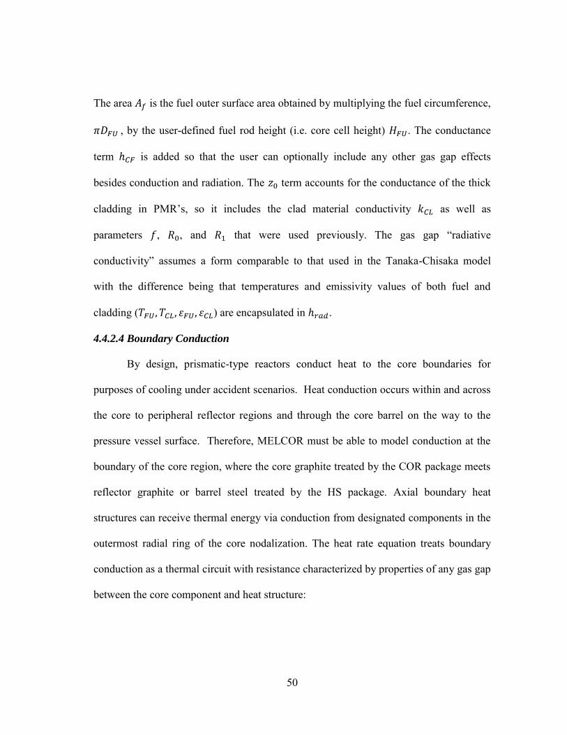
50
The area is the fuel outer surface area obtained by multiplying the fuel circumference,
, by the user-defined fuel rod height (i.e. core cell height) . The conductance
term is added so that the user can optionally include any other gas gap effects
besides conduction and radiation. The term accounts for the conductance of the thick
cladding in PMR’s, so it includes the clad material conductivity as well as
parameters , , and that were used previously. The gas gap “radiative
conductivity” assumes a form comparable to that used in the Tanaka-Chisaka model
with the difference being that temperatures and emissivity values of both fuel and
cladding ( ) are encapsulated in .
4.4.2.4 Boundary Conduction
By design, prismatic-type reactors conduct heat to the core boundaries for
purposes of cooling under accident scenarios. Heat conduction occurs within and across
the core to peripheral reflector regions and through the core barrel on the way to the
pressure vessel surface. Therefore, MELCOR must be able to model conduction at the
boundary of the core region, where the core graphite treated by the COR package meets
reflector graphite or barrel steel treated by the HS package. Axial boundary heat
structures can receive thermal energy via conduction from designated components in the
outermost radial ring of the core nodalization. The heat rate equation treats boundary
conduction as a thermal circuit with resistance characterized by properties of any gas gap
between the core component and heat structure:

51
The first term in the resistance characterizes the resistance of conduction across a gap
of thickness filled with a gas of thermal conductivity . The second term is
included for numerical stability and is called the thermal diffusive resistance. It is a
function of only material properties and the time-step length . The temperature is
the single, average temperature of some general core component C. The temperature
is that of the innermost node for the boundary heat structure in question. Conduction
heat transfer at the core boundary is treated as occurring for 1D slab geometry and not
cylindrical geometry. This is apparent from the definition of the gas gap resistance
because it assumes the familiar form of a plane wall conduction resistance.
4.4.2.5 Convection
Convection heat transfer calculations in the core package occur for every
component that has a user-specified, non-zero surface area. As is always the case with
convection heat transfer, the problem reduces to computing a suitable heat transfer
coefficient for the given flow conditions. The core package proceeds by first computing
four Nusselt (Nu) numbers using various correlations for different possible flow
conditions. This is to say that, regardless of the details of coolant flow, Nu is computed
for cases of forced and free convection in both the laminar and turbulent regimes.
Generally, Nu is correlated in terms of the Reynolds (Re), Prandtl (Pr), and/or Rayleigh
(Ra) numbers. For laminar forced convection, Nu is formulated in terms of a developing

52
flow factor that accounts for entrance effects to the coolant channel. For turbulent forced
convection, the familiar Dittus-Boelter correlation is applied. For both laminar and
turbulent free convection, Nu is written in terms of Ra, the ratio of channel length to
hydraulic diameter, and some empirical constant. There are a few special cases (e.g.
pebble bed convection, boiling, and horizontal surfaces) where only one predetermined
Nu correlation is applied, but these do not factor in to HTGR studies. Thus, two Nu
values are obtained for forced convection and two for free convection. The numerically
largest Nu values for both forced and free convection are identified and taken as
representative of the core flow conditions. The heat transfer coefficient can then be
computed, relaxed by an averaging technique to mitigate potential numerical instability,
and used to compute a convection heat rate between coolant and core components:
The surface area value is that for the component in question (specified in COR input).
The temperature is the single, average value for the core component in question. The
temperature is related to the coolant temperature of the control volume interfacing
with the core cell that contains the core component. However, because it is common
practice to connect multiple axially-adjacent core cells to a single control volume (which
has just one average temperature), the core package uses its “DT/DZ” model in an
attempt to predict an axial temperature gradient within the control volume. The value of

53
results from the DT/DZ model and is a more accurate prediction of local coolant
temperature than the single control volume value.
The DT/DZ model is illustrated in Figure 4.4 for the case of three arbitrarily
numbered core cells coupled to a single representative control volume. An inlet
temperature to the control volume is determined and an energy balance is applied to each
core cell. The balance consists of terms accounting for core cell energy storage across a
time-step, enthalpy flow through the cell, and cell energy sources/sinks (e.g. from
convection cooling of the cell or decay heat generation in the cell). The balance
equations are solved for each cell to construct a rough axial temperature gradient within
the control volume. Evident from Figure 4.4 is the fact that the coolant temperature
calculated for cell 10(X-1) comes from the energy balance equation of cell 10X. Thus
the coolant temperature in any arbitrary cell generally depends on the energy balance of
the cell directly upstream of it (with reference to CVH data for definition of upstream
and downstream). The reader is referred to the MELCOR reference manual for further
information on each of the terms in the balance equation.

54
Figure 4.4. COR package DT/DZ cell-wise energy balance concept [12]

55
5. MELCOR MODELING APPROACH AND
INPUT DEVELOPMENT
5.1 General MELCOR Modeling Approach
A MELCOR model of any general nuclear power system adheres to certain code
requirements that largely dictate modeling approach. The user must appropriately
translate a geometrically complex reactor core in to a simplified 2D cylindrical
representation. The near cylindrical geometry of LWRs lends readily to this
transformation, but the hexagonal/triangular geometry typical of HTGRs does not.
In-core control volume and flow path nodalization follows naturally from the
chosen reactor core nodalization scheme, while ex-core control volumes and flow paths
are often built with other system components in mind (e.g. plenum structures, up-comer
and down-comer regions, steam generator tubes, etc.). The MHTGR and HTTF
MELCOR models are intended only to represent the reactor/facility vessel and
communicating components. Therefore only the active core region, reflector regions,
metallic vessel structures, plenum spaces, inlet/outlet flow ducts, and reactor cavity
cooling system (at least as a boundary condition) are represented in both models.
Appropriate boundary conditions are applied where necessary as a stand-in for omitted
parts of the primary and/or secondary loop. The intent of this section is to explain model
layout and important MHTGR/HTTF input parameters as well as the physical reasoning
behind their definitions. The MHTGR and HTTF input development strategies were
similar, but noteworthy differences will be mentioned when necessary.

56
In general terms, MELCOR model development proceeded as shown in Figure
5.1. An accurate representation of a nuclear system in MELCOR requires access to a
fairly complete design description. This reference could be one or more publications
resembling a design control document wherein the system geometry is described in
sufficient detail. The user must identify system components such as the reactor core and
upper/lower plenum that are important to modeling. Inconsequential system components
should be omitted if possible to avoid undue computational burden.
Figure 5.1. MELCOR input development flow diagram
57
Important system components may or may not need to be broken down to smaller
constituents. Ultimately, such modeling decisions are driven by problem geometry,
problem phenomenology, or other considerations. As an example, the core will likely be
split to axial levels along natural geometric divisions (e.g. the physically separate,
stacked core blocks in the MHTGR) and grouped in radial rings by region (e.g. the solid
center reflector, the active core, the replaceable and permanent side reflector). As further
example, a plenum region could consist of one large control volume or several
connected control volumes if plenum flow modeling is important. The desire to create
consistency between an instrumented test facility and its MELCOR model may also be
an influential factor at this stage.
Once the user has decided which components to include and how best to nodalize
the problem based on modeling goals, the 2D core nodalization can be built. It is at this
stage that geometry transformations occur via conservation of certain geometric
characteristics like cross-sectional area. In this way, hexagonally shaped regions of an
HTGR may be transformed to equivalent circular regions. Each MELCOR core cell
(representing the intersection of a radial ring with an axial level) must be assigned core
components (fuel, cladding, reflector, support structure, etc.) and geometrically
described through specification of cell boundary area, cell cross-sectional flow area,
component equivalent diameters, and component surface areas. Also, each component
with nonzero surface area in each cell must be assigned some material mass. There are
various other required input parameters that relate to core support logic, vessel
geometry, and the fuel/cladding dimensions.

58
After core package input requirements are met, in-core and ex-core control
volumes, flow paths, and heat structures should be added. Because MELCOR performs
hydrodynamic volume consistency checks between core cells and coupled control
volumes, the user must carefully consider the specifications for in-core control volumes.
Also, the in-core flow paths should be geometrically consistent with core flow
parameters. Core axial and radial boundary heat structures should be configured and, in
the case of HTGRs, coupled to the core periphery so as to enable radial heat conduction.
Ex-core control volumes, flow paths, and heat structures should be utilized as necessary
to represent coolant inlets and outlets, upper and lower plena, and time-invariant coolant
sources and sinks (i.e. problem boundary conditions).
After the core, control volumes, flow paths, and heat structures are created,
remaining support functions should be addressed. Any required control logic for
transients must be implemented. Additionally, material properties tables that alter
MELCOR defaults or that characterize entirely new materials must be defined. The user
has enough latitude to incorporate HTGR materials via substitution and redefinition. As
an example, the MELCOR default material properties of zircaloy (one of two possible
materials for the cladding component) might be redefined to match H-451 graphite so
that this material can be used for HTGR modeling.
5.2 Specific MELCOR Modeling Approach
This section deals with specifics of MHTGR and HTTF input development
following the general procedure outlined in Figure 5.1. Because they are similar in many
respects, the approach to modeling was comparable for both systems. Where
appropriate, differences between the two models will be noted.

59
5.2.1 System Design Information
The primary reference for HTTF design details was the most recent collection of
drawings released by OSU [2]. It furnished enough information to create the MELCOR
model and to estimate important quantities like coolant flow area, material mass, etc.
Supplementary sources gave other vital information like anticipated operational
conditions and designer ceramic properties. These sources included a draft copy of the
facility scaling analysis report [3], previous presentations from national conferences or
program review meetings, and direct communications with OSU [2,13].
The MHTGR PSID [1] was the primary reference for MHTGR design details.
Chapters 4 and 5 describing the reactor, the vessel, and the heat transport systems were
frequently referenced for geometric details, normal operating conditions, and other
important information. The component and system drawings were not as complete as
those of the HTTF, so some assumptions about problem geometry were made.
5.2.2 Core Nodalization
The cores of both the MHTGR and HTTF were divided along axial and radial
boundaries to fit within a 2D cylindrical geometry and thus meet MELCOR
requirements. The MHTGR is considerably larger in physical dimensions than the
HTTF, so the two core nodalization schemes are similar but not identical. In both
nodalizations, the axial levels generally correspond to physical elevations where stacked
core elements meet. To satisfy input requirements related to core support logic, the
lower-most level of the upper reflector and the upper-most level of the lower reflector
required special treatment (see section 4.3.4). Radially, a region-wise grouping strategy
was adopted for both systems.

60
Figure 5.2. Geometric transformation of an HTGR core

61
Figure 5.3. COR nodalization of the MHTGR

62
Figure 5.4. COR nodalization of the HTTF

63
Each core ring was associated with a region such as the solid central reflector, the
periphery of the central reflector, a portion of the active core, the inner replaceable side
reflector, the solid side reflector, or the solid/perforated regions of the upper and lower
reflectors. The aforementioned regions are hexagonal as opposed to circular in the real-
world systems, so each was transformed to a circular/annular shape based on
preservation of cross sectional area (which includes structural and flow area). The
number of hexagonal elements within a given region was totaled and multiplied by the
hexagonal area of a single element cross section. The resulting total area was used to
sequentially solve simple equations for ring radii and thereby derive a radial ring
nodalization. This process is illustrated in Figure 5.2 for a general HTGR core.
The MHTGR and HTTF core nodalization diagrams are included in Figures 5.3
and 5.4, respectively. Each diagram represents a vertical half-section view of the
azimuthally symmetric core region. The axial level and radial ring numbers are noted, as
are the core components associated with each core cell. The “null” black regions contain
no COR package materials, but boundary heat structures representing permanent side
reflector graphite actually occupy this physical volume. As is evident from the materials
legend, the MHTGR uses two kinds of graphite in its core and similarly the HTTF uses
two different ceramics in its core. For reasons more fully explained in the facility scaling
analysis report, the HTTF core ceramics are designer materials with customized heat
transport properties that facilitate model-to-prototype similitude.

64
Each model has one or more central reflector rings (rings 1 and 2 in MHTGR,
ring 1 in HTTF), three active core rings (rings 3-5 in MHTGR, rings 2-4 in HTTF), and
one or more replaceable side reflector rings (rings 6-7 in MHTGR, ring 5 in HTTF).
Within a given ring, there are several axial regions. Short descriptions of axial and radial
regions are included in both nodalization diagrams for clarity. The MHTGR has two
rings dedicated to each of the central and replaceable side reflectors, whereas the HTTF
has only one ring dedicated to each of these regions. This is partly because the MHTGR
contains so much more material mass than does the HTTF, but it also facilitates bypass
flow modeling in the MHTGR.
5.2.3 Core Characterization
After devising the core nodalization and defining its geometric boundaries, all
constituent cells must be more completely characterized. Every cell, regardless of its
contents, is described by an outer radius, a bottom elevation, an axial thickness, a
boundary area, and channel/bypass flow areas. Channel and bypass flow areas are
nonzero only if coolant and bypass flow channels are physically present in the cell. Each
cell is optionally assigned one or more core components that each contain one or more
materials. The core components used for MHTGR and HTTF modeling were fuel (FU),
cladding (CL), reflector (RF), and support structure (SS). Each component is described
by an equivalent diameter (i.e. hydraulic diameter), a surface area, and some amount of
material mass. Special components such as RF may require additional information. Any
materials assigned to components have either default or user-specified transport
properties depending on MP package input.

65
Each cell has radial boundaries (inner and outer) and an axial thickness so that
cross-sectional area and boundary area are computed simply as:
These are equations for the annular and cylindrical areas defining a cell. These
parameters help to define not only the nodalization geometry, but also the cell-to-cell
contact areas used to predict conduction and radiation heat transfer between like
components in adjacent cells. Cell flow area is specified by two numbers representing
aggregate channel and bypass flow area. Based on the nodalization, the user should
determine the number of coolant channels in a given core cell and compute the cross-
sectional flow area of one channel. Those two values should be multiplied together to
arrive at the channel flow area of the given core cell. Bypass flow may have several
interpretations depending on the system. In an HTGR, helium may enter gaps between
hexagonal elements or small passages in/around control rod canning to bypass the core.
To estimate bypass flow area, inter-element gap geometry must be examined.

66
Figure 5.5. Channel and bypass flow area for an HTGR fuel element
Multiplying gap flow area by the number of gaps in a core cell yields an approximate
bypass flow area. A simple illustration of bypass and channel flow area in a general
HTGR fuel element is included in Figure 5.5. Because each ring generally consists of
multiple elements (only one of which is pictured in Figure 5.5), a given cell is assigned
flow areas representing sums over several elements. The user should take care to
properly apportion flow area and to avoid double-counting of bypass flow area since
adjacent elements share bypass gaps. The hydrodynamic volume within a core cell is
implied by the channel/bypass flow area and cell height. The product of these two
quantities must at least match the hydrodynamic volume imparted to interfacing control
volumes. It should be noted that convection calculations using bypass flow only occur if

67
two-sided core components (e.g. RF) exist in a core cell, so it is pointless to specify a
bypass flow area for a core cell containing only single-sided components (e.g. CL).
MELCOR characterizes core contents by assigning materials (e.g. zircaloy, UO2)
to components (e.g. clad, fuel). Each core component has a specific purpose and is
handled differently by the core physics models. To apply its heat transfer correlations
and predict energy transfer between components, MELCOR requires a geometric
description of each component in each core cell. The “equivalent diameter” assumes the
conventional definition of a hydraulic diameter (four times the flow area, divided by the
wetted perimeter) and is used to calculate convective heat transfer coefficients. The
component surface area represents that area which would be exposed to coolant and
would be available for convection heat transfer and oxidation. Subject to nodalization
boundaries, the user must specify component mass in each cell.
The interpretation of core components in MELCOR varies with reactor type. For
a PMR-type reactor in MELCOR, the “cladding” actually represents the fuel element
graphite “webbing” in and around the fuel compacts and coolant channels. The
equivalent diameter of “cladding” is simply the coolant channel diameter, while the
surface area in a cell is the total inside area of the coolant channels associated with that
cell. The user must also come up with a “cladding radius”, which is a well-defined
design characteristic in LWRs but is a derived quantity for HTGRs. The graphite
“webbing” should be transformed to an annular region with some effective “cladding
radius” as shown in Figure 5.6.

68
Figure 5.6. Determination of an "effective clad radius" in an HTGR
The reflector component actually replaces the two-sided (channel and bypass)
canister component when a PMR-type reactor is modeled. As with other components, it
requires equivalent diameters and surface areas. However, it requires a pair of values for
each parameter, one for the channel side and one for the bypass side. Also, extra
information specifying reflector geometry (flat plate or cylindrical), thickness, and
orientation (which distinguishes the channel side from the bypass side) is required.
Several miscellaneous parameters describing reactor vessel dimensions and
lower head geometry are required. The vessel input is self-explanatory and the lower
head input, while not arbitrary, is irrelevant to the calculations because lower head
failure is not modeled. A special set of input parameters for prismatic core conduction
heat transfer are more fully described hereafter for clarity. As mentioned in section
4.4.2.2, the Tanaka-Chisaka model is used to compute effective radial core conductivity
69
based on block porosity. The user must compute this porosity from a ratio of
discontinuous volume (helium channels, or “pores”) to continuous (fuel and graphite)
volume. The user must also characterize hexagonal graphite elements by a single
dimension termed the “effective size”, which follows from a simple geometry
transformation. If multiple hexagonal elements comprise the core, a nonzero element-to-
element gap thickness should be specified. MELCOR uses this value to compute an
extra gap conduction resistance term. The MHTGR has several hexagonal elements in
the core, but the HTTF does not. Because of this dissimilarity, there are distinct
differences in radial block conductivity input for the MHTGR and HTTF.
5.2.4 In-Core Input
Within the core, control volumes are coupled to core cells and connected by flow
paths to transport hydrodynamic material. The control volume volume-altitude tables
and flow path geometry should be consistent with core cell input. At the core periphery,
boundary heat structures should be configured for conduction heat transfer.
To establish a link between core structure and hydrodynamic materials, each core
cell must be coupled to a control volume. It is not necessary and is often impractical to
pair a unique control volume with each core cell. Often, the user will choose to assign
several axial levels within a given ring to a single control volume. Thus, the in-core
control volume nodalization usually resembles the core nodalization but is coarser in the
axial direction. The volume-altitude tables of each in-core control volume must still
reflect the axial core nodalization in full detail. Accordingly, there must be an
altitude/volume data pair for each bottom elevation of each core cell interfaced to a
control volume. The discussion of the DT/DZ model in section 4.4.2.5 clarifies the

70
details of convection calculations under this cell-to-volume coupling. MELCOR
performs consistency checks between the hydrodynamic volume specified in volume-
altitude tables and the hydrodynamic volume implied by core package input.
The flow paths connecting in-core control volumes are fully defined by junction
elevations, junction opening heights, flow path area and open fraction, and segmentation
parameters. The “from” and “to” flow path elevations refer to meeting points of
connected control volumes. The flow path length is taken as equal to the center-to-center
distance between interconnected control volumes. The flow path areas should be
consistent with channel or bypass flow areas specified in core package input. If the
information is available, channel surface roughness and forward/reverse loss coefficients
may be specified. In both the HTTF and MHTGR models, only axial flow within coolant
channels or bypass gaps is considered because lateral flow is disallowed by geometry.
Boundary conduction between the outermost core ring and its adjoining heat
structures should be enabled to model conduction from the core. As per MELCOR
requirements, there must be a one-to-one relationship between boundary heat structures
and interfacing core cells so that thermal energy conducted radially within an axial level
is conveyed to a unique heat structure across the core boundary. In the HTTF and
MHTGR models, the outermost core ring consists of replaceable side reflector graphite
while the boundary heat structures consist of permanent side reflector graphite. To
calculate a helium gas gap resistance, a gap thickness between these reflectors was
assumed. Permanent reflector graphite properties were used to compute the thermal
diffusion constant appearing in the boundary conduction equation of section 4.4.2.4.

71
5.2.5 Ex-Core Input
Parts of the system external to the core are created with control volumes, flow
paths, and heat structures. Both the MHTGR and HTTF have upper and lower plena, a
set of up-comer ducts, an outlet duct, an air cavity, and steel structures like the core
barrel, pressure vessel wall, and RCCS panels. Each of these features is discussed below.
Remaining portions of the primary and secondary loops are short-circuited with time-
independent helium source and sink control volumes.
For both models, the upper plenum is treated with three large control volumes
that accept coolant from the up-comer and send coolant to one of many flow paths
leading to the core region. Without several inter-connected control volumes, upper
plenum circulation cannot be modeled in good detail. This is acceptable for purposes of
modeling normal operation or a depressurized conduction cool-down scenario. The
upper plenum appears in Figure 5.7 showing the MHTGR/HTTF ex-core nodalization.
The lower plenum in both models consists of a single, large control volume as
shown in Figure 5.7. Flow exits the core from one of several flow paths and enters the
large plenum to mix/equilibrate before moving to the outlet duct. A finer plenum
nodalization was judged as impractical for purposes of this study because MELCOR
currently does not model air/graphite oxidation reactions. Hence, air ingress and air
circulation in the lower plenum are of no significance and a fine lower plenum
nodalization would only slow the calculation. Furthermore, the effects of graphite
support structures or coolant hot streaks on plenum mixing likely cannot be ascertained
by MELCOR. The plenum dimensions were surmised from design drawings, but plenum
support posts and other miscellaneous structures were not considered.

72
The outlet duct in both models is represented by a single control volume. If air
ingress after a duct break was of concern, a two-volume approach would have been
taken so as to capture counter-current helium/air flow (as occurs during lock-exchange
air ingress). No heat structure surfaces are included as duct walls, though this could be
changed if necessary.
Figure 5.7. Representative CVH nodalization for MHTGR/HTTF

73
An air cavity surrounds the vessel in both models and separates the reactor vessel
wall from the RCCS panels. Radiation occurs across the cavity and it is expected that
some natural air circulation occurs within the cavity. Currently, the cavity is not built to
capture circulation effects since radiation is the dominant vessel heat removal
mechanism. In the event of an outlet duct break, air ingress from the cavity would
commence by molecular diffusion or lock-exchange. The cavity dimensions were
somewhat ambiguous in the literature, so assumptions about geometry were made as
necessary. If a single, large control volume is used, the only important characteristics are
cavity thickness and overall volume.
Steel structures are included in both models. Each system has a core barrel and/or
metallic sleeve structure between the permanent side reflector and the up-comer region.
Up-comer duct metal is not modeled, but the neighboring vessel wall is included and is
“visible” to the core barrel so as to permit radiation heat transfer. The barrel and vessel
walls are modeled with heat structures and are either stainless steel or carbon steel. The
RCCS consists of little more than a set of steel heat structures with a constant-
temperature boundary condition at the outside surface. This is because there is much
uncertainty as to the exact RCCS configuration in the HTTF. As is, the vessel-to-RCCS
view factors or material emissivity values can be varied parametrically.
5.2.6 Ancillary Input
Material substitutions and redefinitions are used extensively in the models. In the
HTTF, core ceramics are specialized to allow for prototype-to-model similitude and
must be completely user-specified. In both models, certain LWR core materials like
zircaloy must be replaced with nuclear grade graphite or a custom ceramic. Also, UO2

74
must be modified to more closely match HTGR fuel compacts or HTTF heater rods. If
necessary, this can be accomplished by assigning multiple materials to the FU
components (e.g. UO2 and porous fuel compact graphite both present in FU).
The HTTF designers at OSU furnished all HTTF materials information, whereas
a previously published graphite materials handbook [14] from General Atomics was
referenced for H451 graphite and 2020 graphite. MELCOR defaults for metallic
materials (carbon steel, stainless steel) were kept unchanged.
Table 5. 1
Ceramic material properties for the MHTGR [14]
T [K] k [W/m*K] T [K] Cp [ J/kg*K]
500.0 115.01 300.0 712.76
600.0 106.13 400.0 990.36
700.0 97.91 500.0 1217.63
800.0 90.34 600.0 1389.86
900.0 83.43 700.0 1519.84
1000.0 77.18 800.0 1619.44
1100.0 71.58 900.0 1697.26
1200.0 66.64 1000.0 1759.23
1300.0 62.36 1100.0 1809.43
1400.0 58.74 1200.0 1850.73
1500.0 55.77 1300.0 1885.16
1600.0 53.45 1400.0 1914.21
1700.0 51.80 1500.0 1938.97
1800.0 50.80 1600.0 1960.27
1700.0 1978.74
1800.0 1994.87
1900.0 2009.05
2000.0 2021.58
2100.0 2032.72
2200.0 2042.65
2300.0 2051.56
2400.0 2059.57
2500.0 2066.79
2600.0 2073.33
2700.0 2079.26
2800.0 2084.66
2900.0 2089.58
3000.0 2094.07
H451 Graphite
T [K] k [W/m*K] T [K] Cp [ J/kg*K]
295.0 62.40 300.0 712.76
473.0 67.20 400.0 990.36
673.0 57.20 500.0 1217.63
873.0 49.80 600.0 1389.86
1073.0 43.90 700.0 1519.84
800.0 1619.44
900.0 1697.26
1000.0 1759.23
1100.0 1809.43
1200.0 1850.73
1300.0 1885.16
1400.0 1914.21
1500.0 1938.97
1600.0 1960.27
1700.0 1978.74
1800.0 1994.87
1900.0 2009.05
2000.0 2021.58
2100.0 2032.72
2200.0 2042.65
2300.0 2051.56
2400.0 2059.57
2500.0 2066.79
2600.0 2073.33
2700.0 2079.26
2800.0 2084.66
2900.0 2089.58
3000.0 2094.07
2020 Graphite

75
Table 5. 2
Ceramic material properties for the HTTF (preliminary data) [13]
The material properties and tabular functions packages were used to specify thermal
conductivity, specific heat capacity, etc. as functions of temperature. Selected materials
data is included in Tables 5.1 and 5.2. MELCOR uses linear interpolation to deduce
material property values when temperature falls between tabular function data points.
Published density values for H-451 and 2020 graphite were not given as functions of
material temperature, so this data was treated as temperature-independent. H-451
graphite density was taken to be 1740.0 kg/m3, whereas 2020 graphite density was
1780.0 kg/m3. The temperature-independent density values for HTTF ceramics are
2971.63 kg/m3 for core-type ceramic and 2954.63 kg/m3 for plenum-type ceramic.
5.2.7 Steady-State and Transient Control Logic
Steady-state boundary conditions consist of source and sink control volumes
connected to the rest of the system with valves and flow paths. The source control
volume is connected with a time-independent flow path so that the incoming coolant
mass flow rate may be user-specified. The thermodynamic conditions of the source
control volume match nominal core inlet conditions, while those of the sink control
volume match expected outlet conditions. Time-independent flow paths were used
between the up-comer and upper plenum control volumes so that bypass flow could be
T [K] k [W/m*K] T [K] Cp [ J/kg*K]
25 4.1 25 428
400 3.9 400 849
985 3.4 985 1078
1315 5 1315 1131
1800 6.5 1800 1173
Core-Type Ceramic
T [K] k [W/m*K] T [K] Cp [ J/kg*K]
25 1.9 25 451
370 1.8 370 876
925 1.6 925 1113
1130 2.1 1130 1149
1320 3.6 1320 1175
Plenum-Type Ceramic

76
split off from coolant channel flow as desired. MELCOR eventually brings the system to
a steady state wherein structure and coolant temperatures no longer change over time.
To model pressurized and depressurized conduction cool-downs in both the
MHTGR and HTTF, some event-initiating control logic was required. For both cases, a
loss of forced circulation must occur at some user-appointed problem time subsequent to
establishment of a steady state. In practice, the LOFC is achieved by changing steady-
state boundary conditions so as to immediately eliminate or quickly coast down the
coolant flow rate from the time-independent source. This LOFC induces a transient state
and sets in motion a PCC or DCC accident sequence. In a PCC, the stagnating coolant
remains in the system at pressure and is able to develop natural circulation patterns.
Thus, for a PCC the source control volume mass flow rate must be immediately forced
to zero or forced to coast down at the time of LOFC. The sink control volume may
remain connected to the system at operating pressure to preclude a depressurization.
Control functions and flow path “valves” may be used to program the PCC. In a DCC,
the system must blow down (i.e. depressurize) through a duct break to the reactor cavity.
Thus, the source and sink control volumes must be isolated and, simultaneously, a flow
path must be opened to the reactor cavity. The depressurization timing may be dictated
by the user (e.g with a CF-controlled linear vessel depressurization) or may be left for
MELCOR to determine. Similar to the PCC, all that is required to implement a DCC are
control functions and flow paths. PCC and DCC control logic is similar for the MHTGR
and HTTF.

77
5.2.8 Decay Heat
For both accident scenarios, intervention of the reactor protection system at the
point of LOFC is assumed. Accordingly, a reactor scram occurs and the core thermal
power immediately transitions to decay heat. As recommended in the OSU scaling
analysis and in accordance with other HTGR computational studies, an ANS standard
decay curve (in MELCOR’s DCH package) was used to calculate decay heat. MHTGR
decay heat is based on a steady-state power level of 350 MW. Because the HTTF heater
rods can achieve an integral power of 2200 kW, a full-scale decay heat profile is
available for experimental purposes. The whole-core decay heat calculation assumes a
long irradiation time before shutdown (584 days) and a certain distribution of fission
power (before shutdown) between three nuclides: 235U, 239Pu, and 238U. The MHTGR
decay heat as predicted from the DCH package is plotted in Figure 5.8 below.
Figure 5.8. DCH package decay heat curve based on ANS standard
0
5
10
15
20
25
0 5 10 15 20
Wh
ole
-Co
re D
eca
y P
ow
er
[MW
]
Time After Shutdown [hr]
Decay Heat Curve for Steady-State Power Level of 350 MW

78
6. RESULTS AND DISCUSSION
Two different systems, the MHTGR and the HTTF, were used to create three
separate test case sets each consisting of three operating scenarios. The MHTGR was
modeled at full power (350 MWth) and at 10% power (35 MWth) with decay heat
calculated by MELCOR accordingly. The HTTF was modeled at its full power level of
2200 kWth with a decay heat curve matching that of the reduced-power MHTGR. Three
operating scenarios were considered for MHTGR models: steady-state, pressurized
conduction cool-down, and depressurized conduction cool-down. Two operating
scenarios were considered for the HTTF model: steady-state and depressurized
conduction cool-down. A more thorough explanation of modeling decisions follows in
the first section of this chapter. The second section presents results of the various
MELCOR calculations, itemized by operating scenario. The third section draws
comparisons of transient response between the reduced-power MHTGR and the HTTF.
The fourth section discusses MELCOR results as they compare to those of RELAP.
6.1 Rationale for Test Case Selection
The choice of modeling a full-power MHTGR, a reduced-power MHTGR, and
the reduced-scale HTTF facilitates comparison of MELCOR predictions to available
RELAP results previously published by INL. Since no HTTF experimental data is
available for a MELCOR-to-experiment benchmark, a RELAP-to-MELCOR comparison
is pursued as the only validation activity currently possible. In accordance with the
methodology of INL, the reduced-power MHTGR model was constructed so that it
featured a one-to-one correspondence to the HTTF in terms of decay power and
temperature. If the general transient response of the full-scale MHTGR resembles that of

79
the reduced-power MHTGR and if, in turn, the general transient response of the reduced-
power MHTGR matches that of the HTTF, one may reasonably conclude that the HTTF
can reproduce full-scale MHTGR phenomena with fair fidelity. Furthermore, one may
gain some measure of confidence in MELCOR modeling capabilities if good agreement
between MELCOR and RELAP is observed.
6.2 MELCOR Predictions
The MELCOR results presented in subsequent sections cover several operating
scenarios for each of the three systems modeled. For the steady-state scenario of each
system, core structure and coolant temperature distributions are included. For the PCC
and DCC scenarios, the predicted time evolution of certain derived quantities (mass-
averaged thermal hydraulics parameters) is presented. For PCC and DCCs in all systems,
instantaneous LOFC is assumed.
6.2.1 MHTGR at 350 MWth
This section presents MELCOR predictions for the full-scale, full-power
MHTGR at steady state and under certain transient/accident conditions. Maps and plots
detailing core structure or coolant temperature distributions comprise the bulk of the
MELCOR results. Certain other noteworthy parameters are mentioned as well.
6.2.1.1 Steady-State
Table 6.1 summarizes some important steady-state characteristics. User-defined
boundary conditions set the specified inlet mass flow rate, temperature, and pressure.

80
Table 6.1
Steady-state parameters for the 350 MWth MHTGR
The desired outlet temperature was achieved if 157.0 kg/s of helium cooled the active
core (rings 3, 4, and 5). For this “channel-side” mass flow rate and for an estimated 10%
bypass flow [1], a total (channel plus bypass) coolant mass flow rate of 174.44 kg/s must
come from the time-independent source control volume.
Table 6.2 is a color-coded core structural temperature map that tabulates the data
plotted in Figure 6.1. Axial levels and radial rings are noted in Table 6.2 (IA/IR), as are
the geometric locations of axial level mid-heights (Z) and radial ring centers (R). The
pressure vessel temperatures are omitted from Figure 6.1. The cladding temperatures of
Table 6.2 (green boxes within the thick black boundaries of the active core) were used to
produce Figure 6.1 as opposed to the fuel temperatures. Note that Figure 6.1d is
basically a color-coded replica of Table 6.2 so that the hotter and cooler regions are
more readily identifiable.
Parameter Value
Power 350 MWth
Coolant Temperature (In | Out) 259.0 ˚C | 685.8 ˚CCoolant flow rate (total | channel) 174.44 kg/s | 157.0 kg/s Bypass flow rate 17.44 kg/s (10%) Inlet Pressure 6.4 MPa

81
Table 6.2
Steady-state core structural temperature map for Figure 6.1 (all temperatures given in ˚C)
IA/IR 1 2 6 7 N1 N2 N3 N4 N5 N6
Z/R [m] 0.25 0.66 1.97 2.27 2.41 2.69 2.96 3.04 3.27 3.40
21 8.72 265.85 263.19 258.93 258.56 249.16 241.97 235.15 232.30
20 8.13 282.03 275.19 258.86 258.36 249.45 241.81 234.61 231.62
19 7.94 294.55 289.64 258.85 258.38 250.96 242.51 234.73 231.55
18 7.53 320.96 319.94 314.31 301.55 311.70 298.92 312.86 300.07 322.04 326.18 288.30 283.92 277.47 274.29
17 6.74 381.21 381.49 426.35 389.31 418.77 381.69 420.88 383.81 376.87 369.01 299.94 292.71 284.56 280.95
16 5.95 451.90 454.23 541.56 483.96 528.71 471.04 531.93 474.26 444.14 423.82 318.06 306.18 295.29 291.00
15 5.16 529.06 534.04 649.68 577.33 631.70 559.22 635.94 563.48 510.48 477.37 337.26 320.19 306.29 301.25
14 4.36 603.91 611.45 741.13 661.26 718.56 638.51 723.61 643.59 568.13 522.62 354.16 332.21 315.57 309.86
13 3.57 663.68 671.98 799.08 719.48 773.74 693.94 779.13 699.36 609.73 555.21 365.76 339.78 320.82 314.54
12 2.78 706.94 716.25 835.72 764.22 807.99 736.19 813.55 741.81 639.03 577.38 374.66 345.94 325.47 318.85
11 1.98 724.54 734.11 838.48 781.80 809.72 752.80 815.09 758.21 650.45 586.04 378.19 348.35 327.29 320.52
10 1.19 713.62 721.68 801.84 765.33 773.94 737.32 778.76 742.17 641.92 580.69 376.42 347.35 326.78 320.15
9 0.40 691.94 696.37 740.87 728.26 714.82 702.17 718.88 706.24 623.76 570.00 371.90 344.17 324.34 317.89
8 -0.01 695.90 698.71 622.39 575.46 493.36 473.80 447.41 435.23
7 -0.30 698.75 700.48 536.11 528.58 493.29 470.69 445.40 434.39
6 -0.79 697.40 699.43 554.76 543.43 502.55 475.96 448.16 436.45
5 -1.19 691.26 693.95 602.01 570.72 487.66 469.47 445.56 434.52
4 -1.69 685.24 689.61 624.96 591.95 496.06 475.66 450.59 439.28
CR Central Reflector Fuel UR Upper Reflector
RSR Replaceable Side Reflector Core Ceramic LR Lower Reflector
PSR Permanent Side Reflector SR/LP Ceramic LP Lower Plenum
CB Core Barrell Core Barrel
RPV Vessel Wall
678.18696.60
684.49
682.61
682.50
706.51
702.81
677.78
677.77
702.44
679.66
Reactor Pressure Vessel
680.21678.20695.11
4 5
681.19
1.640.99 1.31
259.17
259.15
259.15
259.17259.46
260.51
259.56
LRLP
PSR CB RPV
312.89
309.68
187.08
RSRACTIVE CORECR
UR
AC
TIV
E C
OR
E
259.15
259.15
3
189.59
196.80
130.16
272.19
269.41
167.14
169.60
177.70
120.21

82
(a) (b)
(c) (d)
Figure 6.1 Steady-state core structural temperature distribution

83
The axial temperature distribution (Figure 6.1c) is relatively flat in the upper and
lower reflector regions and is consistent with the chopped cosine power profile in the
active core region. Also, the active core distribution is somewhat bottom-peaked with
the hottest reported temperature (excluding fuel) being 781.8 ˚C. In the radial direction
(Figure 6.1b), the central reflector temperature distribution is relatively flat but indicates
the reflector is warmer in the region nearest the active core. This suggests that upon
LOFC, heat conduction to the center of the central reflector will proceed. In the active
core, the innermost region is hotter than the outermost region, which in turn is hotter
than the central region. The replaceable side reflector exhibits a relatively steep radial
temperature gradient, while the permanent side reflector is characterized by a more
gradual temperature gradient. Thus, conduction heat transfer may occur “downhill”
along temperature gradients from the active core to both the central and side reflector.
Table 6.3 shows the steady-state coolant temperatures from the CVH package as
they correspond to core axial levels and radial rings. The coolant enters the upper
reflector at a uniform 259.15 ˚C before entering the core channel/bypass CVs. The active
core uses three CVs per ring (rings 3 to 5) between levels 9 and 18, while the bypass
regions (rings 1, 2, 6, and 7) use only one CV for this same axial level range. All helium
emerges from the core and mixes in the large lower plenum CV so that a coolant
temperature roughly equaling the MHTGR target is achieved.

84
Table 6.3
Steady-state helium temperature map, 350 MWth MHTGR (all temperatures given in ˚C)
6.2.1.2 Pressurized Conduction Cool-Down
At the time of LOFC, an immediate stoppage in coolant flow was imposed by
boundary conditions and the system was opened to a time-independent CV at normal
operating pressure (no breach in the pressure boundary). Also, the core power
transitioned from steady-state to decay heat as would occur after actuation of the reactor
protection system. In the ensuing PCC transient, natural coolant circulation patterns lead
to axial core temperature redistribution from the initial steady state. Also, radial
conduction to the central reflector and core boundary removed residual heat from the
active core region. The transient was run out to a problem time of seven days as this was
enough time for core temperatures to rise, peak, turn over, and begin to decrease.
MELCOR results in this section are presented as mass or area averaged transient
temperature traces for core rings, core levels, and the RPV outer wall. The physical
phenomena encapsulated in each plot are discussed as necessary.
IA/IR 1 2 3 4 5 6 7
UR 19-21 259.15 259.15 259.22 259.15 259.15 259.15 259.15
14-18 481.63 468.38 471.75
11-13 661.08 637.67 642.79
9-10 703.17 677.75 682.61
6-8 703.16 677.77 682.62
4-5 703.07 677.82 682.26
3
2685.77
AC
TIV
E
CO
RE
LRLP
CR ACTIVE CORE RSR
298.85 327.00
692.69 695.44
385.25 314.95
581.99 560.06

85
To observe central reflector heat-up and subsequent radial conduction to the core
periphery, Figure 6.2 showing mass-averaged (by core ring) core graphite temperatures
was created from MELCOR data. The time-to-peak temperature and peak temperature
for each average core ring may be readily obtained from Figure 6.2
Figure 6.2 Mass-averaged (by ring) core graphite temperatures during PCC
The rate of central reflector (R1 and R2) heat-up exceeds that of other rings, and at about
57.2 hr post-LOFC, rings R1 through R3 reach a maximum temperature of
approximately 1028 ˚C. This behavior is consistent with expectations, as the large
inventory of graphite in the central reflector is designed to act as a heat sink for the core

86
under accident conditions. The outer rings R4 through R7 subsequently reach their
respective peak temperatures of 1001 ˚C, 934 ˚C, 861 ˚C, and 805 ˚C at times of 59.5 hr,
65.3 hr, 71.5 hr, and 75.5 hr. Radial conduction from the active core to both the central
and side reflector act to remove residual heat before any damage limits (beginning
around 1650 ˚C) are reached.
Figure 6.3 Mass-averaged (by level) core graphite temperatures during PCC
The effects of natural, density gradient driven helium circulation on axial core
temperature redistribution during a PCC event are noticeable in Figure 6.3. The lower
core structures (L9 through L13) are much warmer than the upper core structures (L14

87
through L18) at the point of LOFC. When forced convection stops, the lower structures
will heat stagnant coolant and cause it to rise towards the cooler upper structures. Thus,
heat is removed from the lower core structures and is effectively relocated by convection
to the upper core structures. All core structures will heat up, but the upper core graphite
will do so at a comparatively greater rate so that the axial core temperature distribution
flattens out from its bottom-peaked steady-state shape. This behavior is evident from
Figure 6.3, as the high rate of temperature increase in L14-L18 and the lower rate of
temperature increase in L9-L13 allows L18 to catch up with L9, L17 to catch up with
L10, etc. The peak temperatures of Figure 6.3 do not coincide with those of Figure 6.2
because level averages were used instead of ring averages to ascertain natural circulation
effects on the axial temperature profile.
As an indirect indicator of passive heat removal from the metallic pressure
vessel, an area average of the RPV outer wall temperature was computed from
MELCOR data. Figure 6.4 shows the result and suggests that radial conduction causes
RPV heat-up and, in turn, increases radiation heat transfer to the RCCS. The RPV outer
wall reaches a maximum temperature of about 291 ˚C at 95.5 hr post-LOFC. It makes
physical sense that the RPV is the last structure to reach its peak temperature because all
thermal energy from inner structures must conduct through and radiate from the RPV to
be removed from the system.

88
Figure 6.4 Area-averaged outer RPV wall temperature during PCC
6.2.1.3 Depressurized Conduction Cool-Down
At the time of LOFC, an immediate stoppage in coolant flow along with a linear,
10 second system depressurization was enforced by system boundary conditions. Also,
the core power transitioned from steady-state to decay heat as would occur after
actuation of the reactor protection system. Subsequently, the system was connected to
time-independent CVs at atmospheric pressure and temperature. In the ensuing DCC
transient, core cooling through the sole mechanism of radial conduction was observed.
The transient was run out to a problem time of seven days as this was enough time for
core temperatures to rise, peak, turn over, and begin to decrease. MELCOR results in

89
this section are presented as mass or area averaged transient temperature traces for core
rings, core levels, and the RPV outer wall. The physical phenomena encapsulated in
each plot are discussed as necessary.
Figure 6.5 shows mass-averaged (by ring) core graphite temperatures during the
DCC in much the same way as Figure 6.2 during the PCC.
Figure 6.5 Mass-averaged (by ring) core graphite temperatures during DCC
The temperature response in Figure 6.5 for the DCC resembles that of the PCC shown
previously because radial conduction remains the most important heat removal
mechanism. For a DCC vs. a PCC, peak temperatures on a ring-to-ring basis tend to be

90
larger by about 200 degrees on average. Additionally, more time is required for core
structural temperatures to peak before leveling off. This difference may be explained by
the absence of circulation effects during the DCC. Because natural circulation cannot act
to remove or redistribute core heat, more thermal energy must be stored in structures as
radial conduction acts to convey thermal energy to the RPV. Hence, more time is
required for conduction heat removal to first catch up with thermal energy storage and
then begin to cool the structures. Rings R1 to R3 reach a peak temperature of 1232 ˚C,
while rings R4 through R7 achieve maximums at 1204 ˚C, 1138 ˚C, 1052 ˚C, and 983
˚C, respectively. Rings R1 to R3 require roughly 69.7 hr to reach maximum temperature,
while rings R4 to R7 need 70.0 hr, 71.4 hr, 77.9 hr, and 82.25 hr, respectively.
Figure 6.6 shows mass-averaged (by level) core structural temperatures during
the DCC. There is no axial temperature profile redistribution due to natural circulation as
occurred in the PCC, so some differences are discernible between Figures 6.6 and 6.3. In
Figure 6.6, the lower levels L9-L13 heat up at a greater rate than in Figure 6.3 because
energy is being stored instead of being removed via natural convection. Because the
lower structures begin at higher temperatures than the upper structures and because
convection does not redistribute thermal energy from the lower core to the upper core,
there is a greater lag in time-to-peak between the upper and lower core. One may then
conclude that the lower core conducts more energy and stores less energy early on in the
DCC transient. This suggests an interesting axial asymmetry with regard to radial core
conduction, as the lower core may be cooling down while the upper core is heating up.

91
Figure 6.6 Mass-averaged (by level) core graphite temperatures during DCC
As an indirect indicator of passive heat removal from the metallic pressure
vessel, an area average of the RPV outer wall temperature was computed from
MELCOR data. Figure 6.6 shows the result and suggests that radial conduction causes
RPV heat-up and, in turn, increases radiation heat transfer to the RCCS. A peak
temperature of 301 ˚C was reached after about 102 hr. Comparing to Figure 6.4, one
notices that the curve in Figure 6.6 exhibits a slight “nose” within 24 hr after the LOFC.
This is likely a consequence of the area-averaging method use to derive the RPV wall
temperature. The upper RPV heat structures have a larger surface area in the MELCOR

92
model. Also, for a DCC the upper core structures store more energy than they conduct
early on in the transient, meaning the upper core periphery stays cooler for a longer time
after LOFC. Hence, the large upper RPV heat structures have cooler temperatures early
on in a DCC, and this causes the area-averaged RPV wall temperature to be cooler.
However, this effect is not purely an artifact of area averaging because it indicates
different axial core temperature distributions in a PCC vs. a DCC shortly after LOFC.
Figure 6.7 Area-averaged outer RPV wall temperature during DCC

93
6.2.2 MHTGR at 35 MWth
This section presents MELCOR predictions for the full-scale, reduced (10%)
power MHTGR at steady state and under certain transient/accident conditions. Maps and
plots detailing core structure or coolant temperature distributions comprise the bulk of
the MELCOR results. Certain other noteworthy parameters are mentioned as well.
6.2.2.1 Steady-State
Table 6.4 summarizes some important steady-state characteristics. User-defined
boundary conditions set the specified inlet mass flow rate, temperature, and pressure.
Because the power was scaled down to 10%, the coolant flow rate was reduced
accordingly to preserve full-scale inlet/outlet coolant temperatures and pressures.
Table 6.4
Steady-state parameters for the 35 MWth MHTGR
The total (channel plus bypass) coolant mass flow rate was reduced by 90.3 % from full
scale in response to the 90% reduction in core power. A 10% bypass flow fraction was
imposed by boundary conditions in keeping with the full-power MHTGR case.
Table 6.5 is a color-coded core structural temperature map that tabulates the data
plotted in Figure 6.2. Axial levels and radial rings are noted in Table 6.5 (IA/IR), as are
Parameter Value
Power 35 MWth
Coolant Temperature (In | Out) 259.15 ˚C | 687.79 ˚CCoolant flow rate (total | channel) 16.85 kg/s | 15.17 kg/s Bypass flow rate 1.685 kg/s (10%) Inlet Pressure 6.4 MPa

94
the geometric locations of axial level mid-heights (Z) and radial ring centers (R). The
pressure vessel temperatures are omitted from Figure 6.8. The cladding temperatures of
Table 6.5 (green boxes within the thick black boundaries of the active core) were used to
produce Figure 6.8 as opposed to the fuel temperatures. Note that Figure 6.8d is a color-
coded replica of Table 6.5 so that hotter and cooler regions are more readily identifiable.
The axial temperature distribution (Figure 6.8c) is relatively flat in the upper and
lower reflector regions and is consistent with the chopped cosine power profile in the
active core region. As was the case at a 350 MWth power, the active core distribution at
35 MWth is somewhat bottom-peaked with the hottest reported temperature (excluding
fuel) being 743.8 ˚C. In the radial direction (Figure 6.8b), the central reflector
temperature distribution is relatively flat but indicates the reflector is warmer in the
region nearest the active core. Generally, structural temperatures on a cell-by-cell basis
are tens of degrees cooler for a 35 MWth power level despite the fact that coolant flow
was adjusted to preserve inlet/outlet helium temperatures. Presumably, this difference
occurs because less thermal energy is stored in the graphite core and reflectors at a lower
steady-state power level. According to Figure 6.8d, the core hot spots remain in
essentially the same geometric locations despite the lowered power level.

95
Table 6.5
Steady-state core structural temperature map for Figure 6.8 (all temperatures given in ˚C)
IA/IR 1 2 6 7 N1 N2 N3 N4 N5 N6
Z/R [m] 0.25 0.662 1.966 2.271 2.413 2.687 2.961 3.037 3.267 3.4
21 8.723 267.19 264.22 258.69 258.35 250.60 247.55 241.80 238.67
20 8.133 283.69 276.60 258.58 258.14 252.00 248.68 242.53 239.18
19 7.935 296.53 291.34 258.58 258.16 251.84 248.02 241.49 237.99
18 7.534 323.03 321.59 299.50 298.45 296.78 295.73 299.97 298.91 322.75 328.31 296.68 292.10 284.09 280.02
17 6.741 375.98 375.31 374.08 371.07 368.14 365.11 369.64 366.62 367.54 363.34 304.23 297.33 288.06 283.72
16 5.948 433.74 434.78 458.22 453.55 449.00 444.30 448.49 443.80 424.43 409.30 316.02 305.24 293.94 289.18
15 5.155 496.40 500.20 543.98 537.88 531.92 525.79 528.75 522.64 481.91 455.04 329.08 313.79 300.17 294.95
14 4.362 557.14 564.25 622.35 615.62 608.24 601.47 601.75 595.00 532.69 494.37 340.60 321.12 305.42 299.80
13 3.569 606.52 614.82 672.27 665.55 657.39 650.64 647.91 641.18 567.13 520.97 347.79 325.07 307.46 301.31
12 2.776 650.12 660.69 722.31 716.28 706.86 700.79 693.37 687.32 596.47 542.11 354.22 328.97 310.17 303.80
11 1.983 675.45 687.03 748.53 743.75 733.46 728.65 716.18 711.40 611.83 553.10 357.55 330.93 311.50 305.02
10 1.189 677.31 687.78 743.67 740.60 729.79 726.71 709.92 706.86 610.37 552.66 357.68 331.22 311.99 305.59
9 0.397 671.14 678.50 721.43 720.37 708.89 707.83 686.87 685.83 600.52 547.53 355.82 330.00 311.09 304.76
8 -0.005 680.91 687.67 599.90 553.01 509.91 491.31 461.77 447.73
7 -0.302 688.07 694.41 532.49 526.99 500.58 481.71 455.77 443.61
6 -0.793 682.41 690.23 547.95 538.90 506.27 483.79 455.93 443.33
5 -1.189 661.13 671.80 589.02 562.02 500.92 485.16 459.27 446.68
4 -1.685 640.61 655.44 607.71 578.47 506.29 488.78 462.38 449.77
CR Central Reflector Fuel UR Upper Reflector
RSR Replaceable Side Reflector Core Ceramic LR Lower Reflector
PSR Permanent Side Reflector SR/LP Ceramic LP Lower Plenum
CB Core Barrell Core Barrel
RPV Reactor Pressure Vessel Vessel Wall
LP
685.76 687.76
LR
712.78 699.40
703.78 692.90
701.80
676.14 686.04
692.59
UR
260.18 259.15 259.15
261.83 259.15 259.15
260.29 259.18 259.17
AC
TIV
E C
OR
E 176.71 157.44
160.44 142.30
158.40 140.31
3 4 5
0.987 1.313 1.639
CR ACTIVE CORE RSR PSR CB RPV
663.46
662.58
674.25
675.01
675.62
268.76312.10
107.78118.42
265.16307.52

96
(a) (b)
(c) (d)
Figure 6.8 Steady-state core structural temperature distribution

97
Table 6.6 shows the steady-state coolant temperatures from the CVH package as
they correspond to core axial levels and radial rings. The coolant enters the upper
reflector at about 259 ˚C before entering the core channel/bypass CVs. The active core
uses three CVs per ring (rings 3 to 5) between levels 9 and 18, while the bypass regions
(rings 1, 2, 6, and 7) use only one CV for this same axial level range. All helium
emerges from the core and mixes in the large lower plenum CV so that a coolant
temperature roughly equaling the MHTGR target is achieved. The active core coolant
temperatures of Table 6.6 are equal to those of Table 6.3 within a few degrees.
Table 6.6
Steady-state helium temperature map, 35 MWth MHTGR (all temperatures given in ˚C)
6.2.2.2 Pressurized Conduction Cool-Down
The same methodology presented in section 6.2.1.2 was applied to the 35 MWth
MHTGR. The PCC transient for this case was similar to that of the 350 MWth as no new
physical phenomena came in to play. The same mass and area averaged quantities are
IA/IR 1 2 3 4 5 6 7
UR 19-21 259.15 259.15 259.96 259.15 259.15 259.15 259.15
14-18 487.24 477.34 474.73
11-13 666.69 652.26 640.65
9-10 706.51 692.83 675.06
6-8 705.33 692.86 674.94
4-5 704.85 691.59 672.51
3
2
LP 687.79
CR ACTIVE CORE RSR
AC
TIV
E
CO
RE
298.85 327.00 385.25 314.95
552.58LR 666.65 676.59 571.26

98
plotted in Figures 6.9 through 6.11, and their respective trajectories through the transient
are seen to agree with Figures 6.2 through 6.4.
Figure 6.9 Mass-averaged (by ring) core graphite temperatures during PCC
The only observable differences in mass-averaged temperatures of Figures 6.9, 6.2, 6.10,
and 6.3 are in peak values. They are lower for the decreased power level, as expected.
The two area-averaged parameters of Figures 6.11 and 6.4 are also different, though very
close, in terms of peak temperature.

99
Figure 6.10 Mass-averaged (by level) core graphite temperatures during PCC

100
Figure 6.11 Area-averaged outer RPV wall temperature for PCC
6.2.2.3 Depressurized Conduction Cool-Down
The same methodology presented in section 6.2.1.3 was applied to the 35 MWth
MHTGR. The DCC transients at 350 MWth and 35 MWth evolved similarly in time,
although peak temperatures were lower and were reached sooner due to the lower
amount of stored energy in the 35 MWth core. Figures 6.12 to 6.15 may be compared
directly to Figures 6.5 to 6.7 to confirm these observations.

101
Figure 6.12 Mass-averaged (by ring) core graphite temperatures during DCC

102
Figure 6.13 Mass-averaged (by level) core graphite temperatures during DCC

103
Figure 6.14 Area-averaged outer RPV wall temperature for DCC
6.2.3 HTTF at 2.2 MWth
This section presents MELCOR predictions for the 2.2 MWth HTTF at steady
state and under DCC transient/accident conditions. Maps and plots detailing core
structure or coolant temperature distributions comprise the bulk of the MELCOR results.
Certain other noteworthy parameters are mentioned as well.
6.2.3.1 Steady-State
Table 6.7 presents some steady-state parameters for the HTTF. No nominal
coolant mass flow rate was available from literature, but with some trial and error
steady-state runs it was determined that 0.96 kg/s of helium was required to reach the

104
target outlet temperatures. Bypass flow was not considered in the HTTF model, but the
actual facility will have control rod sleeve inlet orifices to allow for bypass flow.
Table 6.7
Steady-state parameters for the 2.2 MWth HTTF
Table 6.8 and Figure 6.15 present core temperature maps and plots for the HTTF
at steady-state. HTTF structural temperatures are significantly hotter than those of the
MHTGR, so while full-scale coolant temperature is preserved, structural temperatures
are generally not.
Parameter Value
Power 2.2 MWthCoolant Temperature (In | Out) 260.6 ˚C | 685.1 ˚CCoolant flow rate (total) 0.96 kg/s Inlet Pressure 0.8 MPa

105
Table 6.8
Steady-state core structural temperature map for Figure 6.3 (all temperatures given in ˚C)
CR RSR
IA/IR 1 5 N1 N2 N3 N4 N5 N6
Z/R [m] 0.091 0.539 0.603 0.7 0.743 0.762 0.819 0.832
27 2.329 317.97 337.23 260.49 258.27 256.87 256.18
26 2.2286 568.90 508.10 481.09 318.25 278.89 277.78
25 2.131 572.32 513.44 476.23 317.00 278.09 276.98
24 2.046 568.05 516.80 485.16 320.83 282.64 281.64
23 1.995 556.44 515.40 303.60 261.40 246.17 245.47
22 1.883 518.12 365.05 340.40 369.04 344.38 396.07 371.29 524.30 329.44 280.71 264.47 263.77
21 1.685 558.53 551.73 478.89 570.25 497.22 602.74 529.31 564.46 337.53 282.02 264.96 264.25
20 1.487 610.96 736.78 620.61 770.94 654.14 803.62 686.16 611.74 385.58 323.87 303.11 302.21
19 1.288 662.02 883.67 738.81 920.34 781.08 942.51 806.27 654.20 395.66 325.36 303.63 302.71
18 1.09 706.75 974.34 825.73 1019.22 876.55 1035.30 894.54 690.94 449.75 375.25 348.59 347.43
17 0.892 737.61 1023.32 881.10 1074.13 937.70 1082.90 947.36 713.09 455.63 376.05 348.85 347.68
16 0.694 745.92 1023.40 896.59 1076.56 954.93 1078.14 956.64 717.93 491.40 414.69 383.50 382.13
15 0.496 732.37 979.87 877.80 1033.16 935.33 1027.05 928.76 703.81 487.21 414.08 383.30 381.92
14 0.297 696.29 885.25 816.43 935.33 869.40 922.21 855.56 672.86 492.49 428.01 396.30 394.85
13 0.0991 650.30 750.11 724.33 795.12 770.44 774.47 749.31 634.08 483.11 426.67 395.86 394.42
12 -0.0127 623.13 616.10 471.51 418.57 383.47 381.77
11 -0.089 607.16 549.83 525.41 437.74 395.92 394.14
10 -0.197 610.07 579.10 566.79 450.03 401.42 399.49
9 -0.254 621.30 597.67 433.91 428.64 424.36 422.12
8 -0.381 613.99 602.14 468.90 421.68 390.23 388.71
CR Central Reflector Fuel UR Upper Reflector
RSR Replaceable Side Reflector Core Ceramic LR Lower Reflector
PSR Permanent Side Reflector SR/LP Ceramic LP Lower Plenum
CB Core Barrel Core Barrel
RPV Vessel Wall
UR
263.27
- -
146.17147.53
689.87
627.59 652.90 624.19
668.83
631.27 649.41 634.58
713.78
680.97706.22663.73
656.97678.56
119.87 118.70
125.26126.53
102.60103.54
0.247 0.357 0.438
84.3985.08
71.2171.72
262.10 261.41 264.95
61.4661.99
71.7472.31
262.92 276.60
RPVACTIVE CORE PSR CB
2 3 4
-
333.65
-
654.17
- -
Reactor Pressure Vessel
ACT
IVE
COR
ELR
/FD
B
308.46 319.59

106
(a) (b)
(c) (d)
Figure 6.15 Steady-state core structural temperature distribution

107
The general disagreement between the HTTF and MHTGR in terms of structural
temperatures is likely due to one or more distortions in the relevant scaling ratios defined
by the scaling analysis report [3]. Most likely, the overall core thermal resistance to heat
transfer is not appropriately scaled between the MHTGR and HTTF. This result was not
unexpected, as HTTF heater rod and core ceramic material properties are uncertain.
Thermal conductivity and specific heat capacity are vital components of core thermal
resistance, so if values for these parameters are incorrect one cannot expect similarity.
The axial temperature distribution of Figure 6.15c is more severely peaked than
that of the MHTGR but assumes the same general shape. The radial temperature
distribution of Figure 6.15b appears shifted towards the outer core region. The HTTF hot
spots remain in the lower structure (as in the MHTGR), but are nearer to the periphery.
Table 6.9
Steady-state helium temperature map, HTTF (all temperatures given in ˚C)
CR RSR
IA/IR 1 2 3 4 5
25-27 260.45 260.45 260.32 261.92 261.92
23-24 260.93 260.93 260.81 262.77 262.77
21-22 300.89 300.89 305.30 308.93 308.93
19-20 401.54 401.54 419.01 416.87 416.87
17-18 525.06 525.06 557.98 545.67 545.67
15-16 624.68 624.68 669.00 647.51 647.51
13-14 663.25 663.25 710.66 685.60 685.60
11-12 663.29 663.29 710.52 685.58 685.58
10 663.24 663.24 710.43 685.43 685.43
8-9 663.17 663.17 709.08 684.04 684.04
ACTIVE CORE
AC
TIV
E C
OR
EU
RLR
/FD
BLP 6-7 685.07

108
6.2.3.2 Depressurized Conduction Cool-Down
The only conduction cool-down transient considered for the HTTF was of the
DCC variety, as the facility was not scaled with a PCC in mind. The results of the DCC
include level and ring mass-averaged graphite temperature plots as well as an area-
averaged RPV temperature plot.
Figure 6.16 Mass-averaged (by ring) core graphite temperatures during DCC

109
Figure 6.17 Mass-averaged (by level) core graphite temperatures during DCC

110
Figure 6.18 Area-averaged RPV outer wall temperature for DCC
Figure 6.16 and 6.17 look very comparable to one another in terms of timing and
peak temperature. Hence, the ring and level averages do not differ significantly at any
point in transient time. This suggests that the same kinds of effects attributable to the
bottom-peaked axial temperature distribution in the MHTGR are not preserved in the
HTTF under DCC conditions. In the HTTF, the upper and lower core structural
temperatures seem to increase, level off, and cool down together without any significant
region-wise time lag. This character is not in agreement with MHTGR system response
during a DCC, regardless of power level. The general curve shapes in Figure 6.16 agree
with those of Figure 6.5 apart from the more severe rates of structural heat-up predicted
for the HTTF. This suggests that no new physical phenomena beyond core conduction

111
factor in to DCC event progression of the HTTF. Looking at the average RPV wall
temperature in Figure 6.18, one observes that after about 48 hours the vessel steel begins
to cool off from its peak temperature of 374 ˚C. Thus the RPV of the HTTF gets about
70 degrees hotter than that of the MHTGR but begins to cool off in only half the time.
6.3 Prototype-to-Model Comparison with MELCOR Results
To reiterate previous observations on MHTGR-to-HTTF scaling, poor agreement
was observed under steady-state and DCC conditions, as ring and level mass-averaged
temperature plots showed few similarities. The HTTF design iteration modeled in this
study seems capable of reproducing full-scale MHTGR coolant temperatures, but there
were significant over-predictions in structural temperature. The core temperature
distribution from the MHTGR was not exactly preserved either, as a more center-peaked
axial profile was seen instead of the MHTGR bottom-peaked profile. Because the two
systems were so different at steady-state, DCC transients evolved from dissimilar
starting points and any chance of observing good agreement was lost.
Despite the fact that the same physical phenomena are present in both systems
(forced convection, radial conduction, radiation), a 2.2 MWth HTTF model built with the
latest design information does not scale well with a 350 MWth or 35 MWth MHTGR.
There are simple explanations for this result, namely a lack of preservation in certain
scaling ratios vital to GCR phenomenology. Scaling ratios, especially those related to
conduction heat transfer and thermal energy storage, are strong functions of transport
properties like thermal conductivity and specific heat capacity. If HTTF ceramic
properties have changed from those communicated by OSU some time ago [13] or if

112
further design iterations have altered system characteristics, such revisions are not
accounted for in this study.
Figure 6.19 Ratio of structural temperatures in active core MHTGR-to-HTTF
Figure 6.19 is a map of the active core structural temperature ratios as listed in
Tables 6.2 and 6.8. The temperatures of the MHTGR are divided by those of the HTTF
on a cell-by-cell basis in the active core. Ideally, this ratio would be nearly equal to 1.0
in all cells so as to signify perfect similitude between the two systems. However, Figure
6.19 shows considerable disagreements in most places, especially the lower portions of
the active core.
There were a few encouraging results to be gleaned from MELCOR predictions.
The ring and level average core temperatures in the DCC behaved as expected under
conduction cool-down conditions, as temperatures underwent an excursion to some
maximum before decreasing in a reasonable amount of time. The character of the

113
excursion, turn-over, and drop-off was comparable between the MHTGR and HTTF.
The ratio of time-to-peak temperature under DCC conditions (prototype-to-model) is
roughly 1:2, which is consistent with targets set in the draft scaling analysis report [3].
Furthermore, there is nothing to suggest that MELCOR GCR models are invalid or that
GCR transients cannot be modeled with judicious implementation of boundary
conditions. While there are certain aspects of GCR operation currently beyond the scope
of MELCOR analytical capabilities like plenum hot streaking, air ingress, and
air/graphite oxidation, they can be addressed in the future with new MELCOR models or
with separate effects testing.
6.4 General Assessment of MELCOR/RELAP Agreement
The INL report on analyses of full-scale MHTGR transients was used to draw a
comparison between RELAP and MELCOR predictions of a DCC and PCC. MELCOR
model boundary conditions for a PCC were necessarily adjusted to match those used in
RELAP. A 60 second, linear forced flow coast-down after LOFC was therefore imposed
on the MELCOR PCC. The RELAP analyses use “peak fuel temperature” and RPV
outer wall temperature as metrics to judge response and to contrast the DCC and PCC.
From MELCOR, a mass average of the core cell FU component temperatures in the
hottest core ring was chosen to represent “peak fuel temperature”.

114
Figure 6.20 Hot-ring, mass-averaged FU temperature during PCC and DCC
Comparing Figure 6.20 to Figure 6.21 (reproduced from [4]), one deduces that
MELCOR seems to predict higher “fuel” temperatures than RELAP. Furthermore, it
seems as though the 60 second forced flow coast-down has different effects in RELAP
than it does in MELCOR as far as fuel temperatures are concerned. A significantly larger
dip in fuel temperatures occurs initially in RELAP, presumably because forced cooling
coast down is slower than the transition from operating power to decay heat [4]. The
same occurs in MELCOR, but a much shorter-term fuel cooling effect is observed and
cannot be seen on the time scale of Figure 6.20. The time-to-peak is also different, but
this may be partly due to the mass averaging of MELCOR data.
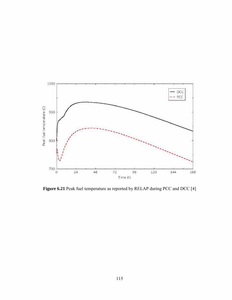
115
Figure 6.21 Peak fuel temperature as reported by RELAP during PCC and DCC [4]

116
Figure 6.22 Area-averaged RPV outer wall temperature during PCC and DCC
An area-averaged RPV wall temperature shown in Figure 6.22 was chosen to
compare with the RELAP RPV temperature in Figure 6.23. As was the case with the fuel
temperature comparison, early stage cooling effects seen in RELAP results are not
present or occur on a much shorter time scale in MELCOR results. The magnitudes of
peak temperatures, while not in excellent agreement, are fairly close considering the
MELCOR result is area-averaged over the entire RPV and the RELAP result is not.

117
Figure 6.23 RPV temperature as reported by RELAP during PCC and DCC
Without a detailed study assessing MELCOR vs. RELAP models, it is difficult to
judge whether differences in core heat transfer models are to blame for the several
discrepancies in results. The RCCS in the MELCOR model was simply a constant-
temperature boundary condition, whereas a more complete air-cooled RCCS may have
been used in the RELAP analyses. Differences in core geometry likely do not contribute
to observed disagreements because the MHTGR PSID was used in the development of
both models. Also, due consideration should be given to material properties. It is unclear
whether the time-dependent thermal conductivity and specific heat capacity values found
in the graphite design handbook [14] are implemented in RELAP as in MELCOR.

118
7. CONCLUSIONS AND RECOMMENDATIONS
MELCOR input decks for both the HTTF and MHTGR were constructed
according to the latest available design references. Using new GCR modeling
capabilities of MELCOR, steady-state and transient cases for both systems were run so
as to predict thermal-hydraulic response. Computational data and general observations of
system behavior were compared to nominal design parameters and to expectations
following from engineering judgment. No code-to-experiment benchmark was possible
because experimental data is as yet unavailable. Several model-to-model and code-to-
code comparisons lead to the conclusion that, while the current MELCOR models
require further revision, MELCOR phenomenological models work as intended to
predict GCR response under steady-state, PCC, and DCC conditions. Most observed
disagreements in prototype-to-model (i.e. MHTGR-to-HTTF) scaling or in MELCOR-
to-RELAP predictions may be explained by and are likely due to factors other than
MELCOR phenomenological modeling. As further information - i.e. a facility
instrumentation plan, a more detailed and complete set of facility drawings, a finalized
set of material properties, etc. - becomes available, the HTTF input may be reconsidered.
There are several issues related to GCR modeling that MELCOR developers at
SNL could work to resolve in the near future. Several improvements dealing with core
support logic, core component material options, oxidation models, and PMR-type fuel
modeling could be made to the COR package for PMR-type reactors. The fact that the
RF component is only self-supporting tends to over-complicate core package input.
Also, if more than two or three materials exist in the core as FU, CL, SS, and RF, the
user is forced to make several materials substitutions and may not be able to

119
accommodate all materials. Air/graphite oxidation and graphite dust transport models are
forthcoming from developers, and incorporation of these models would certainly
enhance code capabilities. Also, an alternative model or method of predicting heat
generation in PMR fuel compacts could increase the fidelity of MELCOR predictions.
However, the developers must wait on such models (empirical or theoretical) to be
created and validated.
When OSU begins testing, SNL might consider building its own models of the
HTTF test matrix. Then, as was done with several other test facilities, the developers
could incorporate this system into the MELCOR automated test suite. Recommendations
for MELCOR users as to best GCR modeling practices would be helpful and could be
developed concurrently. Also, users might benefit from an expanded plotting capability
that includes new variables to indicate core conduction heat transfer and core-to-
structure boundary conduction. At present, the user can only confirm indirectly that
conduction is occurring in the core and at the boundary.

120
REFERENCES
[1] Preliminary Safety Information Document for the Standard MHTGR. Technical Report, HTGR-86-024, Department of Energy, 1986.
[2] S. Cadell, “HTTF Collection”. May 2010. Personal Communication.
[3] B.G. Woods, R.B. Jackson, and B.L. Nelson. Scaling analysis for the very high temperature reactor test facility at Oregon State University. Technical Report DRAFT copy, OSU-VHTR-0001, Oregon State University, February 2009.
[4] Studies related to the Oregon State University high temperature test facility: scaling, the validation matrix, and similarities to the modular high temperature gas-cooled reactor. Technical Report, INL/EXT-10-19803, Idaho National Laboratories, September 2010.
[5] Pre-application safety evaluation report for the modular high temperature gas-cooled reactor (MHTGR). Technical Report, NUREG-1338, U.S. Nuclear Regulatory Commission, December 1995.
[6] K. Kok. Nuclear Engineering Handbook. CRC Press. Boca Raton, FL. 2009.
[7] S.J. Ball and S.E. Fisher. Next generation nuclear plant phenomena identification and ranking tables (PIRTs). Technical Report NUREG/CR-6944, Vol. 2: Accident and Thermal Fluids Analysis, U.S. Nuclear Regulatory Commission, March 2008.
[8] N. Zuber. Appendix D: hierarchical, two-tiered scaling analysis. Technical Report, NUREG/CR-5809, 1991.
[9] S. Basu. Status of the NRC HTGR R&D activities. In Proceedings from the
Cooperative Severe Accident Research Program, Bethesda, MD, September 2009. US Nuclear Regulatory Commission, Rockville, MD.

121
[10] MELCOR Workshop Presentation. In Proceedings from the MELCOR
Workshop, Bethesda, MD, September 2009. U.S. Nuclear Regulatory Commission, Rockville, MD.
[11] MELCOR computer code manuals vol. 1: Primer and users’ guide, version 1.8.6. Technical Report NUREG/CR-6119, Sandia National Laboratories.
[12] MELCOR computer code manuals vol. 2: Reference manual. Technical Report NUREG/CR-6119, Sandia National Laboratories, September 2008.
[13] R.B. Jackson. “HTTF Properties”. January 2011. Personal Communication.
[14] Graphite design handbook. Technical Report, DOE-HTGR-88111, General Atomics, August 1991.
[15] M. Young, “MELCOR equations”. September 2012. Personal Communication.

122
APPENDIX A: MHTGR INPUT/CALCULATION NOTEBOOK
Appendix A contains a package-by-package breakdown of MHTGR MELCOR
input. Tables outlining all input cards, words, and values are included. A brief
explanation of each card is also included where appropriate. Hand calculations based on
the system design description (the MHTGR PSID document) were used to compute
many of the required input parameters. The input below is a representative example for
the MHTGR and represents one of several input deck iterations.
Table A.1
Environmental variables input for MHTGR model
CARD WORD VALUE BASIS
MEG_DIAGFILE - 'mhtgrg.dia' Name of MELGEN diagnostic file MEL_DIAGFILE - 'mhtgr.dia' Name of MELCOR diagnostic file MEG_OUTPUTFILE - 'mhtgrg.out' Name of MELGEN output file MEL_OUTPUTFILE - 'mhtgr.out' Name of MELCOR output file PLOTFILE - 'mhtgr.ptf' Name of plot file MEG_RESTARTFILE - 'mhtgr.rst' Name of MELGEN restart file MEL_RESTARTFILE - mhtgr.rst' Name of MELCOR restart file
CYCLE NCYCLE Restart based on cycle number
NREST -1 Use last available restart dump
MESSAGEFILE - 'mhtgr.mes' Name of message file STATUSFILE - 'MELSTT_v2-0' Name of status file STOPFILE - 'MELSTP_v2-0' Name of stop file WRITENEWINP - 'mhtgr.txt' Name of re-written input file

123
Table A.2
EXEC MELGEN input for MHTGR model
CARD WORD VALUE BASIS
EXEC_INPUT - - Signal start of EXEC input EXEC_TITLE TITLE 'MHTGR' Title of the calculation EXEC_JOBID JOBID 'mhtgr -' Job identifier EXEC_TSTART TSTART -1000 Time at which to start calculation EXEC_SS
-1000 Accelerated steady state run at -1000 seconds
0 Run the accelerated steady state case until time 0
0.01 Take 0.01 s timesteps from -1000 s to 0 s
Table A.3
NCG input for MHTGR model
CARD WORD VALUE BASIS
NCG_INPUT - - Signal start of NCG input NCG_ID MNAME 'HE' Activate helium NCG_ID MNAME 'H2' Activate hydrogen NCG_ID MNAME 'CO' Activate carbon monoxide NCG_ID MNAME 'O2' Activate oxygen NCG_ID MNAME 'CO2' Activate carbon dioxide NCG_ID MNAME 'CH4' Activate CH4 NCG_ID MNAME 'N2' Activate nitrogen

124
Table A.4
CVH input for MHTGR model
CARD WORD VALUE BASIS
CVH_INPUT - - Signal start of CVH input CV_ID CVNAME Table A.4.1 Unique CV name identifier
ICVNUM User-defined CV number
CV_THR ICVTHR NONEQUIL Thermodynamics switch
IPFSW FOG Fog/no fog switch
ICVACT ACTIVE Active/inactive switch
CV_PAS ITYPTH SEPARATE Type of thermodynamic input
IPORA ONLYATM Pool/atmosphere/both switch
VAPORSTATE SUPERHEATED Thermo. state of CV atmosphere
CV_PTD PTDID PVOL Keyword for CV pressure
PVOL 6.40E+06 Initial CV pressure
CV_AAD ATMID TATM Keyword for CV atm. temperature
TATM 763.15 Initial atmosphere temperature
CV_NCG NMMAT
Table A.4.1
Number of NCG materials
NCGID Keyword Identifier, RHUM for all
VALUE
Value from key, 0.0 = RHUM for all
NUM Table row index
NAMGAS NCG MELCOR name
MLFR Mole fraction of NCG in CV
CV_VAT ICVVZP Table A.4.2
Number of volume/altitude data pairs
NCVZ Table row index
CVZ Altitude of current data pair
CVVOL Volume of current data pair

125
Table A.4.1
CV_NCG for MHTGR model
CV_ID CV_NCG
CVNAME ICVNUM NMMAT NCGID VALUE NUM NAMGAS MLFR
DUMMY_IA1 100 1 RHUM 0.0 1 HE 1.0 LH_CV 101 1 RHUM 0.0 1 HE 1.0 LP_1_2 102 1 RHUM 0.0 1 HE 1.0 LP_1_3 103 1 RHUM 0.0 1 HE 1.0 POST_FDB_1 104 1 RHUM 0.0 1 HE 1.0 LR_1 105 1 RHUM 0.0 1 HE 1.0 CORE_1_1 106 1 RHUM 0.0 1 HE 1.0 CORE_1_2 107 1 RHUM 0.0 1 HE 1.0 CORE_1_3 108 1 RHUM 0.0 1 HE 1.0 UR_1 109 1 RHUM 0.0 1 HE 1.0 LP_2_2 202 1 RHUM 0.0 1 HE 1.0 LP_2_3 203 1 RHUM 0.0 1 HE 1.0 POST_FDB_2 204 1 RHUM 0.0 1 HE 1.0 LR_2 205 1 RHUM 0.0 1 HE 1.0 CORE_2_1 206 1 RHUM 0.0 1 HE 1.0 CORE_2_2 207 1 RHUM 0.0 1 HE 1.0 CORE_2_3 208 1 RHUM 0.0 1 HE 1.0 UR_2 209 1 RHUM 0.0 1 HE 1.0 LP_3_2 302 1 RHUM 0.0 1 HE 1.0 LP_3_3 303 1 RHUM 0.0 1 HE 1.0 POST_FDB_3 304 1 RHUM 0.0 1 HE 1.0 LR_3 305 1 RHUM 0.0 1 HE 1.0 CORE_3_1 306 1 RHUM 0.0 1 HE 1.0 CORE_3_2 307 1 RHUM 0.0 1 HE 1.0 CORE_3_3 308 1 RHUM 0.0 1 HE 1.0 UR_3 309 1 RHUM 0.0 1 HE 1.0 LP_4_2 402 1 RHUM 0.0 1 HE 1.0 LP_4_3 403 1 RHUM 0.0 1 HE 1.0 POST_FDB_4 404 1 RHUM 0.0 1 HE 1.0 LR_4 405 1 RHUM 0.0 1 HE 1.0 CORE_4_1 406 1 RHUM 0.0 1 HE 1.0 CORE_4_2 407 1 RHUM 0.0 1 HE 1.0 CORE_4_3 408 1 RHUM 0.0 1 HE 1.0 UR_4 409 1 RHUM 0.0 1 HE 1.0 LP_5_2 502 1 RHUM 0.0 1 HE 1.0

126
LP_5_3 503 1 RHUM 0.0 1 HE 1.0 POST_FDB_5 504 1 RHUM 0.0 1 HE 1.0 LR_5 505 1 RHUM 0.0 1 HE 1.0 CORE_5_1 506 1 RHUM 0.0 1 HE 1.0 CORE_5_2 507 1 RHUM 0.0 1 HE 1.0 CORE_5_3 508 1 RHUM 0.0 1 HE 1.0 UR_5 509 1 RHUM 0.0 1 HE 1.0 LP_6_2 602 1 RHUM 0.0 1 HE 1.0 LP_6_3 603 1 RHUM 0.0 1 HE 1.0 POST_FDB_6 604 1 RHUM 0.0 1 HE 1.0 LR_6 605 1 RHUM 0.0 1 HE 1.0 CORE_6_1 606 1 RHUM 0.0 1 HE 1.0 CORE_6_2 607 1 RHUM 0.0 1 HE 1.0 CORE_6_3 608 1 RHUM 0.0 1 HE 1.0 UR_6 609 1 RHUM 0.0 1 HE 1.0 LP_7_2 702 1 RHUM 0.0 1 HE 1.0 LP_7_3 703 1 RHUM 0.0 1 HE 1.0 POST_FDB_7 704 1 RHUM 0.0 1 HE 1.0 LR_7 705 1 RHUM 0.0 1 HE 1.0 CORE_7_1 706 1 RHUM 0.0 1 HE 1.0 CORE_7_2 707 1 RHUM 0.0 1 HE 1.0 CORE_7_3 708 1 RHUM 0.0 1 HE 1.0 UR_7 709 1 RHUM 0.0 1 HE 1.0 UPPER_PLENUM 800 1 RHUM 0.0 1 HE 1.0 LOWER_DUCT 801 1 RHUM 0.0 1 HE 1.0 UPPER_DUCT 802 1 RHUM 0.0 1 HE 1.0 SINK 803 1 RHUM 0.0 1 HE 1.0 SOURCE 804 1 RHUM 0.0 1 HE 1.0 CAVITY_1 901 2 RHUM 0.0 2
N2 O2
0.8 0.2
CAVITY_2 902 2 RHUM 0.0 2 CAVITY_3 903 2 RHUM 0.0 2 CAVITY_4 904 2 RHUM 0.0 2 CAVITY_5 905 2 RHUM 0.0 2 CAVITY_6 906 2 RHUM 0.0 2

127
Table A.4.2
CV_VAT for MHTGR model
CV_ID CV_VAT
CVNAME ICVNUM ICVVZP NCVZ CVZ CVVOL BASIS
DUMMY_IA1 100 2 1 -6.28250 0.0 Bottom of Z1
2 -2.88250 3.0395E+01 Top of Z1, nominal LH_CV 101 2 1 -6.28250 0.0
Dummy for COR 2 -2.88250 1.0000E+01 LP_1_2 102 2 1 -2.88250 0.0 Bottom of Z2
2 -2.43250 -3.5343E-01 IR 1, IA 2 LP_1_3 103 2 1 -2.43250 0.0 Bottom of Z3
2 -1.98250 -3.5343E-01 IR 1, IA 3 POST_FDB_1 104 3 1 -1.98250 0.0 Bottom of Z4
2 -1.38775 -1.4833E-04 IR 1, IA 4
3 -0.99125 -9.8890E-05 IR 1, IA 5 LR_1 105 4 1 -0.99125 0.0 Bottom of Z6
2 -0.59475 -9.8890E-05 IR 1, IA 6
3 -0.01000 -1.4584E-04 IR 1, IA 7
4 0.00000 -2.4940E-06 IR 1, IA 8 CORE_1_1 106 3 1 0.00000 0.0 Bottom of Z9
2 0.79300 -1.9780E-04 IR 1, IA 9
3 1.58600 -1.9780E-04 IR 1, IA 10 CORE_1_2 107 4 1 1.58600 0.0 Bottom of Z11
2 2.37900 -1.9780E-04 IR 1, IA 11
3 3.17200 -1.9780E-04 IR 1, IA 12
4 3.96500 -1.9780E-04 IR 1, IA 13 CORE_1_3 108 6 1 3.96500 0.0 Bottom of Z14
2 4.75800 1.9800E-04 IR 1, IA 14
3 5.55100 1.9800E-04 IR 1, IA 15
4 6.34400 1.9800E-04 IR 1, IA 16
5 7.13700 1.9800E-04 IR 1, IA 17
6 7.93000 1.9800E-04 IR 1, IA 18 UR_1 109 4 1 7.93000 0.0 Bottom of Z19
2 7.94000 -2.4940E-06 IR 1, IA 19
3 8.32650 -9.6393E-05 IR 1, IA 20
4 9.11950 -1.9780E-04 IR 1, IA 21 LP_2_2 202 2 1 -2.88250 0.0 Bottom of Z2
2 -2.43250 -6.0590E-01 IR 2, IA 2 LP_2_3 203 2 1 -2.43250 0.0 Bottom of Z3

128
2 -1.98250 -6.0590E-01 IR 2, IA 3 POST_FDB_2 204 3 1 -1.98250 0.0 Bottom of Z4
2 -1.38775 -3.7080E-04 IR 2, IA 4
3 -0.99125 -2.4720E-04 IR 2, IA 5 LR_2 205 4 1 -0.99125 0.0 Bottom of Z6
2 -0.59475 -2.4720E-04 IR 2, IA 6
3 -0.01000 -3.6453E-04 IR 2, IA 7
4 0.00000 -6.2340E-06 IR 2, IA 8 CORE_2_1 206 3 1 0.00000 0.0 Bottom of Z9
2 0.79300 -4.9440E-04 IR 2, IA 9
3 1.58600 -4.9440E-04 IR 2, IA 10 CORE_2_2 207 4 1 1.58600 0.0 Bottom of Z11
2 2.37900 -4.9440E-04 IR 2, IA 11
3 3.17200 -4.9440E-04 IR 2, IA 12
4 3.96500 -4.9440E-04 IR 2, IA 13 CORE_2_3 208 6 1 3.96500 0.0 Bottom of Z14
2 4.75800 -4.9440E-04 IR 2, IA 14
3 5.55100 -4.9440E-04 IR 2, IA 15
4 6.34400 -4.9440E-04 IR 2, IA 16
5 7.13700 -4.9440E-04 IR 2, IA 17
6 7.93000 -4.9440E-04 IR 2, IA 18 UR_2 209 4 1 7.93000 0.0 Bottom of Z19
2 7.94000 -6.2300E-06 IR 2, IA 19
3 8.32650 -2.4094E-04 IR 2, IA 20
4 9.11950 -4.9440E-04 IR 2, IA 21 LP_3_2 302 2 1 -2.88250 0.0 Bottom of Z2
2 -2.43250 -9.0882E-01 IR 3, IA 2 LP_3_3 303 2 1 -2.43250 0.0 Bottom of Z3
2 -1.98250 -9.0882E-01 IR 3, IA 3 POST_FDB_3 304 3 1 -1.98250 0.0 Bottom of Z4
2 -1.38775 -1.5553E-01 IR 3, IA 4
3 -0.99125 -1.0370E-01 IR 3, IA 5 LR_3 305 4 1 -0.99125 0.0 Bottom of Z6
2 -0.59475 -1.3743E-01 IR 3, IA 6
3 -0.01000 -2.0267E-01 IR 3, IA 7
4 0.00000 -3.4660E-03 IR 3, IA 8 CORE_3_1 306 3 1 0.00000 0.0 Bottom of Z9
2 0.79300 -2.7490E-01 IR 3, IA 9
3 1.58600 -2.7490E-01 IR 3, IA 10

129
CORE_3_2 307 4 1 1.58600 0.0 Bottom of Z11
2 2.37900 -2.7490E-01 IR 3, IA 11
3 3.17200 -2.7490E-01 IR 3, IA 12
4 3.96500 -2.7490E-01 IR 3, IA 13 CORE_3_3 308 6 1 3.96500 0.0 Bottom of Z14
2 4.75800 -2.7490E-01 IR 3, IA 14
3 5.55100 -2.7490E-01 IR 3, IA 15
4 6.34400 -2.7490E-01 IR 3, IA 16
5 7.13700 -2.7490E-01 IR 3, IA 17
6 7.93000 -2.7490E-01 IR 3, IA 18 UR_3 309 4 1 7.93000 0.0 Bottom of Z19
2 7.94000 -3.4660E-03 IR 3, IA 19
3 8.32650 -1.3396E-01 IR 3, IA 20
4 9.11950 -2.7485E-01 IR 3, IA 21 LP_4_2 402 2 1 -2.88250 0.0 Bottom of Z2
2 -2.43250 -1.2118E+00 IR 4, IA 2 LP_4_3 403 2 1 -2.43250 0.0 Bottom of Z3
2 -1.98250 -1.2118E+00 IR 4, IA 3 POST_FDB_4 404 3 1 -1.98250 0.0 Bottom of Z4
2 -1.38775 -3.1099E-01 IR 4, IA 4
3 -0.99125 -2.0733E-01 IR 4, IA 5 LR_4 405 4 1 -0.99125 0.0 Bottom of Z6
2 -0.59475 -1.9995E-01 IR 4, IA 6
3 -0.01000 -2.4940E-01 IR 4, IA 7
4 0.00000 5.0430E-03 IR 4, IA 8 CORE_4_1 406 3 1 0.00000 0.0 Bottom of Z9
2 0.79300 -3.9991E-01 IR 4, IA 9
3 1.58600 -3.9991E-01 IR 4, IA 10 CORE_4_2 407 4 1 1.58600 0.0 Bottom of Z11
2 2.37900 -3.9991E-01 IR 4, IA 11
3 3.17200 -3.9991E-01 IR 4, IA 12
4 3.96500 -3.9991E-01 IR 4, IA 13 CORE_4_3 408 6 1 3.96500 0.0 Bottom of Z14
2 4.75800 -3.9991E-01 IR 4, IA 14
3 5.55100 -3.9991E-01 IR 4, IA 15
4 6.34400 -3.9991E-01 IR 4, IA 16
5 7.13700 -3.9991E-01 IR 4, IA 17
6 7.93000 -3.9991E-01 IR 4, IA 18 UR_4 409 4 1 7.93000 0.0 Bottom of Z19

130
2 7.94000 -5.0430E-03 IR 4, IA 19
3 8.32650 -1.9491E-01 IR 4, IA 20
4 9.11950 -3.9991E-01 IR 4, IA 21 LP_5_2 502 2 1 -2.88250 0.0 Bottom of Z2
2 -2.43250 -1.5147E+00 IR 5, IA 2 LP_5_3 503 2 1 -2.43250 0.0 Bottom of Z3
2 -1.98250 -1.5147E+00 IR 5, IA 3 POST_FDB_5 504 3 1 -1.98250 0.0 Bottom of Z4
2 -1.38775 -3.1099E-01 IR 5, IA 4
3 -0.99125 -2.0733E-01 IR 5, IA 5 LR_5 505 4 1 -0.99125 0.0 Bottom of Z6
2 -0.59475 -1.9995E-01 IR 5, IA 6
3 -0.01000 -2.9490E-01 IR 5, IA 7
4 0.00000 -5.0430E-03 IR 5, IA 8 CORE_5_1 506 3 1 0.00000 0.0 Bottom of Z9
2 0.79300 -3.9991E-01 IR 5, IA 9
3 1.58600 -3.9991E-01 IR 5, IA 10 CORE_5_2 507 4 1 1.58600 0.0 Bottom of Z11
2 2.37900 -3.9991E-01 IR 5, IA 11
3 3.17200 -3.9991E-01 IR 5, IA 12
4 3.96500 -3.9991E-01 IR 5, IA 13 CORE_5_3 508 6 1 3.96500 0.0 Bottom of Z14
2 4.75800 -3.9991E-01 IR 5, IA 14
3 5.55100 -3.9991E-01 IR 5, IA 15
4 6.34400 -3.9991E-01 IR 5, IA 16
5 7.13700 -3.9991E-01 IR 5, IA 17
6 7.93000 -3.9991E-01 IR 5, IA 18 UR_5 509 4 1 7.93000 0.0 Bottom of Z19
2 7.94000 -5.0430E-03 IR 5, IA 19
3 8.32650 -1.9491E-01 IR 5, IA 20
4 9.11950 -3.9991E-01 IR 5, IA 21 LP_6_2 602 2 1 -2.88250 0.0 Bottom of Z2
2 -2.43250 -1.8176E+00 IR 6, IA 2 LP_6_3 603 2 1 -2.43250 0.0 Bottom of Z3
2 -1.98250 -1.8176E+00 IR 6, IA 3 POST_FDB_6 604 3 1 -1.98250 0.0 Bottom of Z4
2 -1.38775 -1.4213E-03 IR 6, IA 4
3 -0.99125 -9.4752E-04 IR 6, IA 5 LR_6 605 4 1 -0.99125 0.0 Bottom of Z6

131
2 -0.59475 -9.4752E-04 IR 6, IA 6
3 -0.01000 -1.3974E-03 IR 6, IA 7
4 0.00000 -2.3897E-05 IR 6, IA 8 CORE_6_1 606 3 1 0.00000 0.0 Bottom of Z9
2 0.79300 -1.8950E-03 IR 6, IA 9
3 1.58600 -1.8950E-03 IR 6, IA 10 CORE_6_2 607 4 1 1.58600 0.0 Bottom of Z11
2 2.37900 -1.8950E-03 IR 6, IA 11
3 3.17200 -1.8950E-03 IR 6, IA 12
4 3.96500 -1.8950E-03 IR 6, IA 13 CORE_6_3 608 6 1 3.96500 0.0 Bottom of Z14
2 4.75800 -1.8950E-03 IR 6, IA 14
3 5.55100 -1.8950E-03 IR 6, IA 15
4 6.34400 -1.8950E-03 IR 6, IA 16
5 7.13700 -1.8950E-03 IR 6, IA 17
6 7.93000 -1.8950E-03 IR 6, IA 18 UR_6 609 4 1 7.93000 0.0 Bottom of Z19
2 7.94000 -2.3897E-05 IR 6, IA 19
3 8.32650 -9.2362E-04 IR 6, IA 20
4 9.11950 -1.8950E-03 IR 6, IA 21 LP_7_2 702 2 1 -2.88250 0.0 Bottom of Z2
2 -2.43250 -1.8176E+00 IR 7, IA 2 LP_7_3 703 2 1 -2.43250 0.0 Bottom of Z3
2 -1.98250 -1.8176E+00 IR 7, IA 3 POST_FDB_7 704 3 1 -1.98250 0.0 Bottom of Z4
2 -1.38775 -1.4090E-03 IR 7, IA 4
3 -0.99125 -9.3930E-04 IR 7, IA 5 LR_7 705 4 1 -0.99125 0.0 Bottom of Z6
2 -0.59475 -9.3930E-04 IR 7, IA 6
3 -0.01000 -1.3852E-03 IR 7, IA 7
4 0.00000 -2.3690E-05 IR 7, IA 8 CORE_7_1 706 3 1 0.00000 0.0 Bottom of Z9
2 0.79300 -1.8790E-03 IR 7, IA 9
3 1.58600 -1.8790E-03 IR 7, IA 10 CORE_7_2 707 4 1 1.58600 0.0 Bottom of Z11
2 2.37900 -1.8790E-03 IR 7, IA 11
3 3.17200 -1.8790E-03 IR 7, IA 12
4 3.96500 -1.8790E-03 IR 7, IA 13 CORE_7_3 708 6 1 3.96500 0.0 Bottom of Z14

132
2 4.75800 -1.8790E-03 IR 7, IA 14
3 5.55100 -1.8790E-03 IR 7, IA 15
4 6.34400 -1.8790E-03 IR 7, IA 16
5 7.13700 -1.8790E-03 IR 7, IA 17
6 7.93000 -1.8790E-03 IR 7, IA 18 UR_7 709 4 1 7.93000 0.0 Bottom of Z19
2 7.94000 -2.3689E-05 IR 7, IA 19
3 8.32650 -9.1560E-04 IR 7, IA 20
4 9.11950 -1.8790E-03 IR 7, IA 21 UPPER_PLENUM 800 2 1 9.11950 0.0000E+00 Top of UR
2 12.15630 2.9419E+01 Half volume of sphere with RCOR
LOWER_DUCT 801 2 1 -2.88250 0.0000E+00
2 -2.28750 1.5350E+00 Half of horizontal cylinder hot duct
UPPER_DUCT 802 2 1 -2.28750 0.0000E+00
2 -1.69250 1.5350E+00 Half of horizontal cylinder hot duct
UPCOMER 805 2 1 -1.98250 0.0000E+00
2 11.53200 1.6269E+01 12 ducts, 6" by 26" = 0.152 m by 0.66 m
CAVITY_1 901 2 1 -1.98250 0.0000E+00 2 -0.99125 2.4290E+01 1 m thick cavity CAVITY_2 902 2 1 -0.99125 0.0000E+00 2 0.00000 2.4290E+01 1 m thick cavity CAVITY_3 903 2 1 0.00000 0.0000E+00 2 1.58600 3.8860E+01 1 m thick cavity CAVITY_4 904 2 1 1.58600 0.0000E+00 2 3.96500 5.8290E+01 1 m thick cavity CAVITY_5 905 2 1 3.96500 0.0000E+00 2 7.93000 9.7160E+01 1 m thick cavity CAVITY_6 906 2 1 7.93000 0.0000E+00 2 9.11950 2.9150E+01 1 m thick cavity

133
Table A.5
FL input for MHTGR model
CARD WORD VALUE BASIS
FL_INPUT - - Signal start of FL input FL_ID FPNAME
Table A.5.1
FL name
IFPNUM User-defined FL number
FL_FT KCVFM Name of "from" control volume
KCVTO Name of "to" control volume
ZFM Altitude of "from" junction
ZTO Altitude of "to" junction
FL_GEO FLARA
Table A.5.2
Flow path area
FLLEN Flow path length
FLOPO Flow path open fraction
FLHGTF Junction opening height, "from"
FLHGTT Junction opening height, "to"
FL_JSW KFLGFL Flow path orientation (0 = vertical, 3 = horizontal) FL_SEG IPNSG Number of segments
NSEG Table row index
SAREA Segment flow area
SLEN Segment flow length
SHYD Segment hydraulic diameter
FL_VTM NVOFT 1 Number of time-dependent flow paths
NFLT 1 Table row index
FLNAME SRC_to_UPCOMER Name of time-dependent flow path
NTFLAG CF Flag for CF or TF defining velocity vs. time
NFUN VELOCITY Name of CF or TF

134
Table A.5.1
FL_FT for MHTGR model
FL_ID
FL_FT
FPNAME IFPNUM
KCVFM KCVTO ZFM ZTO
UR_1_to_CORE_1_3 101
UR_1 CORE_1_3 7.930 7.930
CORE_1_3_to_1_2 102
CORE_1_3 CORE_1_2 3.965 3.965
CORE_1_2_to_1_1 103
CORE_1_2 CORE_1_1 1.586 1.586
CORE_1_1_to_LR_1 104
CORE_1_1 LR_1 0.000 0.000
LR_1_to_POST_FDB_1 105
LR_1 POST_FDB_1 -0.991 -0.991
UR_2_to_CORE_2_3 201
UR_2 CORE_2_3 7.930 7.930
CORE_2_3_to_2_2 202
CORE_2_3 CORE_2_2 3.965 3.965
CORE_2_2_to_2_1 203
CORE_2_2 CORE_2_1 1.586 1.586
CORE_2_1_to_LR_2 204
CORE_2_1 LR_2 0.000 0.000
LR_2_to_POST_FDB_2 205
LR_2 POST_FDB_2 -0.991 -0.991
UR_3_to_CORE_3_3 301
UR_3 CORE_3_3 7.930 7.930
CORE_3_3_to_3_2 302
CORE_3_3 CORE_3_2 3.965 3.965
CORE_3_2_to_3_1 303
CORE_3_2 CORE_3_1 1.586 1.586
CORE_3_1_to_LR_3 304
CORE_3_1 LR_3 0.000 0.000
LR_3_to_POST_FDB_3 305
LR_3 POST_FDB_3 -0.991 -0.991
UR_4_to_CORE_4_3 401
UR_4 CORE_4_3 7.930 7.930
CORE_4_3_to_4_2 402
CORE_4_3 CORE_4_2 3.965 3.965
CORE_4_2_to_4_1 403
CORE_4_2 CORE_4_1 1.586 1.586
CORE_4_1_to_LR_4 404
CORE_4_1 LR_4 0.000 0.000
LR_4_to_POST_FDB_4 405
LR_4 POST_FDB_4 -0.991 -0.991
UR_5_to_CORE_5_3 501
UR_5 CORE_5_3 7.930 7.930
CORE_5_3_to_5_2 502
CORE_5_3 CORE_5_2 3.965 3.965
CORE_5_2_to_5_1 503
CORE_5_2 CORE_5_1 1.586 1.586
CORE_5_1_to_LR_5 504
CORE_5_1 LR_5 0.000 0.000
LR_5_to_POST_FDB_5 505
LR_5 POST_FDB_5 -0.991 -0.991
UR_6_to_CORE_6_3 601
UR_6 CORE_6_3 7.930 7.930
CORE_6_3_to_6_2 602
CORE_6_3 CORE_6_2 3.965 3.965
CORE_6_2_to_6_1 603
CORE_6_2 CORE_6_1 1.586 1.586
CORE_6_1_to_LR_6 604
CORE_6_1 LR_6 0.000 0.000
LR_6_to_POST_FDB_6 605
LR_6 POST_FDB_6 -0.991 -0.991
UR_7_to_CORE_7_3 701
UR_7 CORE_7_3 7.930 7.930
CORE_7_3_to_7_2 702
CORE_7_3 CORE_7_2 3.965 3.965
CORE_7_2_to_7_1 703
CORE_7_2 CORE_7_1 1.586 1.586
CORE_7_1_to_LR_7 704
CORE_7_1 LR_7 0.000 0.000
LR_7_to_POST_FDB_7 705
LR_7 POST_FDB_7 -0.991 -0.991
POST_FDB_1_to_LP_1_3 106
POST_FDB_1 LP_1_3 -1.983 -1.983
LP_1_3_to_LP_1_2 107
LP_1_3 LP_1_2 -2.433 -2.433

135
POST_FDB_2_to_LP_2_3 206
POST_FDB_2 LP_2_3 -1.983 -1.983
LP_2_3_to_LP_2_2 207
LP_2_3 LP_2_2 -2.433 -2.433
POST_FDB_3_to_LP_3_3 306
POST_FDB_3 LP_3_3 -1.983 -1.983
LP_3_3_to_LP_3_2 307
LP_3_3 LP_3_2 -2.433 -2.433
POST_FDB_4_to_LP_4_3 406
POST_FDB_4 LP_4_3 -1.983 -1.983
LP_4_3_to_LP_4_2 407
LP_4_3 LP_4_2 -2.433 -2.433
POST_FDB_5_to_LP_5_3 506
POST_FDB_5 LP_5_3 -1.983 -1.983
LP_5_3_to_LP_5_2 507
LP_5_3 LP_5_2 -2.433 -2.433
POST_FDB_6_to_LP_6_3 606
POST_FDB_6 LP_6_3 -1.983 -1.983
LP_6_3_to_LP_6_2 607
LP_6_3 LP_6_2 -2.433 -2.433
POST_FDB_7_to_LP_7_3 706
POST_FDB_7 LP_7_3 -1.983 -1.983
LP_7_3_to_LP_7_2 707
LP_7_3 LP_7_2 -2.433 -2.433
LP_1_3_to_2_3 1001
LP_1_3 LP_2_3 -2.208 -2.208
LP_1_2_to_2_2 1002
LP_1_2 LP_2_2 -2.433 -2.433
LP_2_3_to_3_3 2001
LP_2_3 LP_3_3 -2.208 -2.208
LP_2_2_to_3_2 2002
LP_2_2 LP_3_2 -2.433 -2.433
LP_3_3_to_4_3 3001
LP_3_3 LP_4_3 -2.208 -2.208
LP_3_2_to_4_2 3002
LP_3_2 LP_4_2 -2.433 -2.433
LP_4_3_to_5_3 4001
LP_4_3 LP_5_3 -2.208 -2.208
LP_4_2_to_5_2 4002
LP_4_2 LP_5_2 -2.433 -2.433
LP_5_3_to_6_3 5001
LP_5_3 LP_6_3 -2.208 -2.208
LP_5_2_to_6_2 5002
LP_5_2 LP_6_2 -2.433 -2.433
LP_6_3_to_7_3 6001
LP_6_3 LP_7_3 -2.208 -2.208
LP_6_2_to_7_2 6002
LP_6_2 LP_7_2 -2.433 -2.433
to_up_duct 801
LP_7_3 UPPER_DUCT -2.208 -2.208
to_lwr_duct 802
LP_7_2 LOWER_DUCT -2.433 -2.433
up_duct_to_snk 803
UPPER_DUCT SINK -2.208 -2.208
lwr_duct_to_snk 804
LOWER_DUCT SINK -2.433 -2.433
UP_to_R1 111
UPPER_PLENUM UR_1 9.120 9.120
UP_to_R2 112
UPPER_PLENUM UR_2 9.120 9.120
UP_to_R3 113
UPPER_PLENUM UR_3 9.120 9.120
UP_to_R4 114
UPPER_PLENUM UR_4 9.120 9.120
UP_to_R5 115
UPPER_PLENUM UR_5 9.120 9.120
UP_to_R6 116
UPPER_PLENUM UR_6 9.120 9.120
UP_to_R7 117
UPPER_PLENUM UR_7 9.120 9.120
SRC_to_UPCOMER 120
SOURCE UPCOMER 0.000 0.000
UPCOMER_to_UP 121
UPCOMER UPPER_PLENUM 10.32 10.32

136
Table A.5.2
FL geometric parameters for MHTGR model
FPNAME FLARA FLLEN FLOPO KFLGFL SAREA SLEN SHYD
UR_1_to_CORE_1_3 2.4940E-04 2.577 1.0 0 2.4940E-04 2.577 1.9900E-05
CORE_1_3_to_1_2 2.4940E-04 3.172 1.0 0 2.4940E-04 3.172 1.9900E-05
CORE_1_2_to_1_1 2.4940E-04 1.983 1.0 0 2.4940E-04 1.983 1.9900E-05
CORE_1_1_to_LR_1 2.4940E-04 1.289 1.0 0 2.4940E-04 1.289 1.9900E-05
LR_1_to_POST_FDB_1 2.4940E-04 0.991 1.0 0 2.4940E-04 0.991 1.9900E-05
UR_2_to_CORE_2_3 6.2340E-04 2.577 1.0 0 6.2340E-04 2.577 1.9900E-05
CORE_2_3_to_2_2 6.2340E-04 3.172 1.0 0 6.2340E-04 3.172 1.9900E-05
CORE_2_2_to_2_1 6.2340E-04 1.983 1.0 0 6.2340E-04 1.983 1.9900E-05
CORE_2_1_to_LR_2 6.2340E-04 1.289 1.0 0 6.2340E-04 1.289 1.9900E-05
LR_2_to_POST_FDB_2 6.2340E-04 0.991 1.0 0 6.2340E-04 0.991 1.9900E-05
UR_3_to_CORE_3_3 3.4660E-01 2.577 1.0 0 3.4660E-01 2.577 1.5900E-02
CORE_3_3_to_3_2 3.4660E-01 3.172 1.0 0 3.4660E-01 3.172 1.5900E-02
CORE_3_2_to_3_1 3.4660E-01 1.983 1.0 0 3.4660E-01 1.983 1.5900E-02
CORE_3_1_to_LR_3 3.4660E-01 1.289 1.0 0 3.4660E-01 1.289 1.5900E-02
LR_3_to_POST_FDB_3 2.6150E-01 0.992 1.0 0 3.4660E-01 0.496 1.5900E-02
UR_4_to_CORE_4_3 5.0430E-01 2.577 1.0 0 5.0430E-01 2.577 1.5900E-02
CORE_4_3_to_4_2 5.0430E-01 3.172 1.0 0 5.0430E-01 3.172 1.5900E-02
CORE_4_2_to_4_1 5.0430E-01 1.983 1.0 0 5.0430E-01 1.983 1.5900E-02
CORE_4_1_to_LR_4 5.0430E-01 1.289 1.0 0 5.0430E-01 1.289 1.5900E-02
LR_4_to_POST_FDB_4 5.0430E-01 0.992 1.0 0 5.0430E-01 0.496 1.5900E-02
UR_5_to_CORE_5_3 5.0430E-01 2.577 1.0 0 5.0430E-01 2.577 1.5900E-02
CORE_5_3_to_5_2 5.0430E-01 3.172 1.0 0 5.0430E-01 3.172 1.5900E-02
CORE_5_2_to_5_1 5.0430E-01 1.983 1.0 0 5.0430E-01 1.983 1.5900E-02
CORE_5_1_to_LR_5 5.0430E-01 1.289 1.0 0 5.0430E-01 1.289 1.5900E-02
LR_5_to_POST_FDB_5 5.0430E-01 0.992 1.0 0 5.0430E-01 0.496 1.5900E-02
UR_6_to_CORE_6_3 2.3897E-03 2.577 1.0 0 2.3897E-03 2.577 1.9900E-05
CORE_6_3_to_6_2 2.3897E-03 3.172 1.0 0 2.3897E-03 3.172 1.9900E-05
CORE_6_2_to_6_1 2.3897E-03 1.983 1.0 0 2.3897E-03 1.983 1.9900E-05
CORE_6_1_to_LR_6 2.3897E-03 1.289 1.0 0 2.3897E-03 1.289 1.9900E-05
LR_6_to_POST_FDB_6 2.3897E-03 0.992 1.0 0 2.3897E-03 0.992 1.9900E-05
UR_7_to_CORE_7_3 2.3689E-03 2.577 1.0 0 2.3689E-03 2.577 1.9900E-05
CORE_7_3_to_7_2 2.3689E-03 3.172 1.0 0 2.3689E-03 3.172 1.9900E-05
CORE_7_2_to_7_1 2.3689E-03 1.983 1.0 0 2.3689E-03 1.983 1.9900E-05
CORE_7_1_to_LR_7 2.3689E-03 1.289 1.0 0 2.3689E-03 1.289 1.9900E-05
LR_7_to_POST_FDB_7 2.3689E-03 0.992 1.0 0 2.3689E-03 0.992 1.9900E-05
POST_FDB_1_to_LP_1_3 7.8540E-01 0.721 1.0 0 7.8540E-01 0.721 1.0000E+00
LP_1_3_to_LP_1_2 7.8540E-01 0.450 1.0 0 7.8540E-01 0.450 1.0000E+00
POST_FDB_2_to_LP_2_3 1.3464E+00 0.721 1.0 0 1.3464E+00 0.721 1.5280E+00

137
LP_2_3_to_LP_2_2 1.3464E+00 0.450 1.0 0 1.3464E+00 0.450 1.5280E+00
POST_FDB_3_to_LP_3_3 2.0196E+00 0.721 1.0 0 2.0196E+00 0.721 3.9460E+00
LP_3_3_to_LP_3_2 2.0196E+00 0.450 1.0 0 2.0196E+00 0.450 3.9460E+00
POST_FDB_4_to_LP_4_3 2.6928E+00 0.721 1.0 0 2.6928E+00 0.721 5.2510E+00
LP_4_3_to_LP_4_2 2.6928E+00 0.450 1.0 0 2.6928E+00 0.450 5.2510E+00
POST_FDB_5_to_LP_5_3 3.3660E+00 0.721 1.0 0 3.3660E+00 0.721 6.5570E+00
LP_5_3_to_LP_5_2 3.3660E+00 0.450 1.0 0 3.3660E+00 0.450 6.5570E+00
POST_FDB_6_to_LP_6_3 4.0392E+00 0.721 1.0 0 4.0392E+00 0.721 7.8660E+00
LP_6_3_to_LP_6_2 4.0392E+00 0.450 1.0 0 4.0392E+00 0.450 7.8660E+00
POST_FDB_7_to_LP_7_3 4.0392E+00 0.721 1.0 0 4.0392E+00 0.721 9.0860E+00
LP_7_3_to_LP_7_2 4.0392E+00 0.450 1.0 0 4.0392E+00 0.450 9.0860E+00
LP_1_3_to_2_3 1.4137E+00 0.412 1.0 3 1.4137E+00 0.412 9.0000E-01
LP_1_2_to_2_2 1.4137E+00 0.412 1.0 3 1.4137E+00 0.412 9.0000E-01
LP_2_3_to_3_3 2.3292E+00 0.488 1.0 3 2.3292E+00 0.488 9.0000E-01
LP_2_2_to_3_2 2.3292E+00 0.488 1.0 3 2.3292E+00 0.488 9.0000E-01
LP_3_3_to_4_3 3.2504E+00 0.327 1.0 3 3.2504E+00 0.327 9.0000E-01
LP_3_2_to_4_2 3.2504E+00 0.327 1.0 3 3.2504E+00 0.327 9.0000E-01
LP_4_3_to_5_3 4.1736E+00 0.327 1.0 3 4.1736E+00 0.327 9.0000E-01
LP_4_2_to_5_2 4.1736E+00 0.327 1.0 3 4.1736E+00 0.327 9.0000E-01
LP_5_3_to_6_3 5.0976E+00 1.118 1.0 3 5.0976E+00 1.118 9.0000E-01
LP_5_2_to_6_2 5.0976E+00 1.118 1.0 3 5.0976E+00 1.118 9.0000E-01
LP_6_3_to_7_3 6.0219E+00 0.635 1.0 3 6.0219E+00 0.635 9.0000E-01
LP_6_2_to_7_2 6.0219E+00 0.635 1.0 3 6.0219E+00 0.635 9.0000E-01
to_up_duct 5.5610E-01 2.000 1.0 3 5.5610E-01 2.000 2.9080E+00
to_lwr_duct 5.5610E-01 2.000 1.0 3 5.5610E-01 2.000 2.9080E+00
up_duct_to_snk 5.5610E-01 2.000 1.0 3 5.5610E-01 2.000 2.9080E+00
lwr_duct_to_snk 5.5610E-01 2.000 1.0 3 5.5610E-01 2.000 2.9080E+00
UP_to_R1 2.4940E-04 1.801 1.0 0 2.4940E-04 1.801 1.9900E-05
UP_to_R2 6.2340E-04 1.801 1.0 0 6.2340E-04 1.801 1.9900E-05
UP_to_R3 3.4660E-01 1.801 1.0 0 3.4660E-01 1.801 1.5900E-02
UP_to_R4 5.0430E-01 1.801 1.0 0 5.0430E-01 1.801 1.5900E-02
UP_to_R5 5.0430E-01 1.801 1.0 0 5.0430E-01 1.801 1.5900E-02
UP_to_R6 2.3897E-03 1.801 1.0 0 2.3897E-03 1.801 1.9900E-05
UP_to_R7 2.3689E-03 1.801 1.0 0 2.3689E-03 1.801 1.9900E-05
SRC_to_UPCOMER 1.2040E+00 1.000 1.0 0 1.2040E+00 1.000 2.9660E+00
UPCOMER_to_UP 1.2040E+00 1.000 1.0 3 1.2040E+00 1.000 2.9660E+00

138
Table A.6
HS input for MHTGR model
CARD WORD VALUE BASIS
HS_INPUT - - Signal start of HS input HS_ID HSNAME
Table A.6.1
HS name
NUM User-defined HS number HS_GD IGEOM HS geometry HS_EOD HSALT HS bottom elevation
ALPHA HS orientation HS_SRC ISRC NO Internal Power Source Flag HS_ND NP
Table A.6.1
Number of temperature nodes
N Node index
XI Spatial node location
MATNAM Material name associated with node N HS_LB IBCL CALCCOEFHS Boundary condition type
IBVL Table A.6.2 Boundary control volume name
MTEVAL NO Switch to evaluate mass transfer at boundary HS_LBP IFLOWL INT Internal/external flow flag
CPFPL 0.0 Critical pool fraction
CPFAL 0.0 Critical pool fraction for atmosphere HS_LBF IOPTL
Table A.6.2 Fluid temperature options for LHS
NUMAXL Axial level of coupled core cell if necessary
NUMRAD Radial ring of coupled core cell if necessary HS_LBS ASURFL 1.0 LHS area, calculate internally for cylinders
CLNL Table A.6.2
LHS characteristic length, cylinder height
BNDZL Heat structure LHS boundary height, cylinder height
HS_LBR EMISWL 0.8 Surface material emissivity (LHS)
RMODL EQUIV-BAND Radiation model flag (LHS)
PATHL 0.0508 Radiation path length (LHS) HS_RB for RHS , See HS_LB
Table A.6.3 Same as HS_LB, but for RHS
HS_RBR for RHS , See HS_LBR Same as HS_LBR, but for RHS
HS_RBP for RHS , See HS_LBP Table A.6.3
Same as HS_LBP, but for RHS
HS_RBS for RHS , See HS_LBS Same as HS_LBS, but for RHS
HS_FT IFTNUM OFF Film tracking on/off switch

139
Table A.6.1
HS geometric parameters for MHTGR model
HSNAME NUM IGEOM HSALT ALPHA NP N XI MATNAM
LPbnd_2 102 CYLINDRICAL -2.8825 1.0 3 1 2.4128 ALUMINUM
2 2.9608 ALUMINUM
3 3.0368 CARBSTEEL
LPbnd_3 103 CYLINDRICAL -2.4325 1.0 3 1 2.4128 ALUMINUM
2 2.9608 ALUMINUM
3 3.0368 CARBSTEEL
PBbnd_4 104 CYLINDRICAL -1.9825 1.0 3 1 2.4128 ALUMINUM
2 2.9608 ALUMINUM
3 3.0368 CARBSTEEL
FDBbnd_5 105 CYLINDRICAL -1.3878 1.0 3 1 2.4128 ALUMINUM
2 2.9608 ALUMINUM
3 3.0368 CARBSTEEL
LRbnd_6 106 CYLINDRICAL -0.9913 1.0 3 1 2.4128 ALUMINUM
2 2.9608 ALUMINUM
3 3.0368 CARBSTEEL
LRbnd_7 107 CYLINDRICAL -0.5948 1.0 3 1 2.4128 ALUMINUM
2 2.9608 ALUMINUM
3 3.0368 CARBSTEEL
LRbnd_8 108 CYLINDRICAL -0.0100 1.0 3 1 2.4128 ALUMINUM
2 2.9608 ALUMINUM
3 3.0368 CARBSTEEL
SRCB_9 109 CYLINDRICAL 0.0000 1.0 3 1 2.4128 ALUMINUM
2 2.9608 ALUMINUM
3 3.0368 CARBSTEEL
SRCB_10 110 CYLINDRICAL 0.7930 1.0 3 1 2.4128 ALUMINUM
2 2.9608 ALUMINUM
3 3.0368 CARBSTEEL
SRCB_11 111 CYLINDRICAL 1.5860 1.0 3 1 2.4128 ALUMINUM
2 2.9608 ALUMINUM
3 3.0368 CARBSTEEL
SRCB_12 112 CYLINDRICAL 2.3790 1.0 3 1 2.4128 ALUMINUM
2 2.9608 ALUMINUM
3 3.0368 CARBSTEEL
SRCB_13 113 CYLINDRICAL 3.1720 1.0 3 1 2.4128 ALUMINUM
2 2.9608 ALUMINUM
3 3.0368 CARBSTEEL
SRCB_14 114 CYLINDRICAL 3.9650 1.0 3 1 2.4128 ALUMINUM
2 2.9608 ALUMINUM

140
3 3.0368 CARBSTEEL
SRCB_15 115 CYLINDRICAL 4.7580 1.0 3 1 2.4128 ALUMINUM
2 2.9608 ALUMINUM
3 3.0368 CARBSTEEL
SRCB_16 116 CYLINDRICAL 5.5510 1.0 3 1 2.4128 ALUMINUM
2 2.9608 ALUMINUM
3 3.0368 CARBSTEEL
SRCB_17 117 CYLINDRICAL 6.3440 1.0 3 1 2.4128 ALUMINUM
2 2.9608 ALUMINUM
3 3.0368 CARBSTEEL
SRCB_18 118 CYLINDRICAL 7.1370 1.0 3 1 2.4128 ALUMINUM
2 2.9608 ALUMINUM
3 3.0368 CARBSTEEL
URbnd_19 119 CYLINDRICAL 7.9300 1.0 3 1 2.4128 ALUMINUM
2 2.9608 ALUMINUM
3 3.0368 CARBSTEEL
URbnd_20 120 CYLINDRICAL 7.9400 1.0 3 1 2.4128 ALUMINUM
2 2.9608 ALUMINUM
3 3.0368 CARBSTEEL
URbnd_21 121 CYLINDRICAL 8.3265 1.0 3 1 2.4128 ALUMINUM
2 2.9608 ALUMINUM
3 3.0368 CARBSTEEL
UP_TPS 122 HEMISPHERE 9.1195 1.0 2 1 2.9608 SS304
2 3.0368 SS304
RPV_1 201 CYLINDRICAL -1.9825 1.0 2 1 3.267 SS304
2 3.4 SS304
RPV_2 202 CYLINDRICAL -0.9913 1.0 2 1 3.267 SS304
2 3.4 SS304
RPV_3 203 CYLINDRICAL 0.0000 1.0 2 1 3.267 SS304
2 3.4 SS304
RPV_4 204 CYLINDRICAL 1.5860 1.0 2 1 3.267 SS304
2 3.4 SS304
RPV_5 205 CYLINDRICAL 3.9650 1.0 2 1 3.267 SS304
2 3.4 SS304
RPV_6 206 CYLINDRICAL 7.9300 1.0 2 1 3.267 SS304
2 3.4 SS304

141
Table A.6.2
HS LHS boundary conditions for MHTGR model
HSNAME IBVL IOPTL NUMAXL NUMRAD CLNL BNDZL
LPbnd_2 LP_7_2 DTDZ 2 7 0.45000 0.45000
LPbnd_3 LP_7_3 DTDZ 3 7 0.45000 0.45000
PBbnd_4 POST_FDB_7 DTDZ 4 7 0.59475 0.59475
FDBbnd_5 POST_FDB_7 DTDZ 5 7 0.39650 0.39650
LRbnd_6 LR_7 DTDZ 6 7 0.39650 0.39650
LRbnd_7 LR_7 DTDZ 7 7 0.58475 0.58475
LRbnd_8 LR_7 DTDZ 8 7 0.01000 0.01000
SRCB_9 CORE_7_1 DTDZ 9 7 0.79300 0.79300
SRCB_10 CORE_7_1 DTDZ 10 7 0.79300 0.79300
SRCB_11 CORE_7_2 DTDZ 11 7 0.79300 0.79300
SRCB_12 CORE_7_2 DTDZ 12 7 0.79300 0.79300
SRCB_13 CORE_7_2 DTDZ 13 7 0.79300 0.79300
SRCB_14 CORE_7_3 DTDZ 14 7 0.79300 0.79300
SRCB_15 CORE_7_3 DTDZ 15 7 0.79300 0.79300
SRCB_16 CORE_7_3 DTDZ 16 7 0.79300 0.79300
SRCB_17 CORE_7_3 DTDZ 17 7 0.79300 0.79300
SRCB_18 CORE_7_3 DTDZ 18 7 0.79300 0.79300
URbnd_19 UR_7 DTDZ 19 7 0.01000 0.01000
URbnd_20 UR_7 DTDZ 20 7 0.38650 0.38650
URbnd_21 UR_7 DTDZ 21 7 0.79300 0.79300
UP_TPS UPPER_PLENUM - - - 1.00000 3.03680
RPV_1 UPCOMER - - - 0.99125 0.99125
RPV_2 UPCOMER - - - 0.99125 0.99125
RPV_3 UPCOMER - - - 1.58600 1.58600
RPV_4 UPCOMER - - - 2.37900 2.37900
RPV_5 UPCOMER - - - 3.17200 3.17200
RPV_6 UPCOMER - - - 1.18950 1.18950

142
Table A.6.3
HS RHS boundary conditions for MHTGR model
HSNAME IBCR IBVR IFLOWR CPFPL CPFAL CLNR BNDZR
LPbnd_2 SYMMETRY NO INT 0.0 0.0 0.45000 0.45000
LPbnd_3 SYMMETRY NO INT 0.0 0.0 0.45000 0.45000
PBbnd_4 CALCCOEFHS UPCOMER INT 0.0 0.0 0.59475 0.59475
FDBbnd_5 CALCCOEFHS UPCOMER INT 0.0 0.0 0.39650 0.39650
LRbnd_6 CALCCOEFHS UPCOMER INT 0.0 0.0 0.39650 0.39650
LRbnd_7 CALCCOEFHS UPCOMER INT 0.0 0.0 0.58475 0.58475
LRbnd_8 CALCCOEFHS UPCOMER INT 0.0 0.0 0.01000 0.01000
SRCB_9 CALCCOEFHS UPCOMER INT 0.0 0.0 0.79300 0.79300
SRCB_10 CALCCOEFHS UPCOMER INT 0.0 0.0 0.79300 0.79300
SRCB_11 CALCCOEFHS UPCOMER INT 0.0 0.0 0.79300 0.79300
SRCB_12 CALCCOEFHS UPCOMER INT 0.0 0.0 0.79300 0.79300
SRCB_13 CALCCOEFHS UPCOMER INT 0.0 0.0 0.79300 0.79300
SRCB_14 CALCCOEFHS UPCOMER INT 0.0 0.0 0.79300 0.79300
SRCB_15 CALCCOEFHS UPCOMER INT 0.0 0.0 0.79300 0.79300
SRCB_16 CALCCOEFHS UPCOMER INT 0.0 0.0 0.79300 0.79300
SRCB_17 CALCCOEFHS UPCOMER INT 0.0 0.0 0.79300 0.79300
SRCB_18 CALCCOEFHS UPCOMER INT 0.0 0.0 0.79300 0.79300
URbnd_19 CALCCOEFHS UPCOMER INT 0.0 0.0 0.01000 0.01000
URbnd_20 CALCCOEFHS UPCOMER INT 0.0 0.0 0.38650 0.38650
URbnd_21 CALCCOEFHS UPCOMER INT 0.0 0.0 0.79300 0.79300
UP_TPS SYMMETRY NO EXT 0.0 0.0 1.00000 3.03680
RPV_1 CALCCOEFHS CAVITY_1 EXT 0.5 0.5 0.99125 0.99125
RPV_2 CALCCOEFHS CAVITY_2 EXT 0.5 0.5 0.99125 0.99125
RPV_3 CALCCOEFHS CAVITY_3 EXT 0.5 0.5 1.58600 1.58600
RPV_4 CALCCOEFHS CAVITY_4 EXT 0.5 0.5 2.37900 2.37900
RPV_5 CALCCOEFHS CAVITY_5 EXT 0.5 0.5 3.17200 3.17200
RPV_6 CALCCOEFHS CAVITY_6 EXT 0.5 0.5 1.18950 1.18950

143
Table A.7
COR input for MHTGR model
COR_INPUT - - Signal start of COR input COR_RT IRTYP PMR Reactor type flag
MCRP B4C Poison material (insignificant for this calculation) COR_GP RFUEL 0.006225 Fuel rod (i.e. fuel compact) outer radius
RCLAD 0.00863 Clad outer radius
DRGAP 1.25E-04 Gap thickness between fuel/clad
PITCH 0.0188 Fuel rod (i.e. fuel compact) center-to-center distance COR_VP RCOR 2.4128 Outer radius for active core region
RVESS 3.4 Inner radius of vessel
ILHTRN RVESS LH transition type (inconsequential in this calculation)
DZRV 0.133 Vessel wall thickness
DZLH 0.133 LH thickness (inconsequential in this calculation)
ILHTYP HEMISPHERE LH geometry (inconsequential in this calculation)
RVLH 3.4 For hemispherical lower head, radius of curvature COR_AVP HLST -2.8825 Elevation below which the lower head models apply
HCSP -2.8825 Elevation of core support plate, > HLST COR_TP NTPCOR NO TP name for CAV/FDI (inconsequential)
RNTPCOR NO TP name for radionuclides (inconsequential)
ICFGAP NO FU/CL gap conductance CF name (inconsequential)
ICFFIS FISPOWALL Fission power CF, FISPOWALL = whole-core power
CFNAME CORE-POWER CF name giving fission power COR_MS IEUMOD 0 Materials interactions model switch (inconsequential)
IHSDT 0 HS boundary switch, set to DT/DZ model
IDTDZ 0 DT/DZ inlet specification option switch
ICORCV 1 COR/CVH hydrodynamic volume consistency switch COR_BCP ICBCD CB Component Mnemonic for conducting core component
MATBCD HE Gap material separating core and the heat structures
DXBCD 1.00E-04 Gap thickness
CDFBCD 1.58E-04 Thermal diffusion constant COR_CLM CLMAT GRAPH Identifier for cladding material COR_RFM RFMAT GRAPH Identifier for reflector material COR_FUM XFUMAT INC Identifier for fuel "extra", inconel is compact graphite COR_LP IAXSUP 2 Axial level containing support plate (inconsequential)
HDBH2O 100 HTC from in-vessel falling debris to (inconsequential)
PPFAIL 2.00E+07 Differential pressure for LH failure (inconsequential)
VFALL 1 Falling debris velocity (inconsequential) COR_TKE TKETF NO Name of TF for effective conductivity, if used

144
PORCHAN 0.2369 Eff. block porosity used in Tanaka-Chisaka model
DBLK 0.378 Effective graphite block size for gap model
BLKGAP 0.0001 Gap width between graphite blocks for gap model COR_LH NLH 2 Number of LH temperature nodes (inconsequential)
NINSLH 0 Number of insulation mesh layers (inconsequential) COR_EDV ITEMP 1 Temperature edit flag
IMASS 1 Mass edit flag
IVOL 1 Volume edit flag
IASUR 1 Surface area edit flag
IPMV 1 Component masses plot flag
IPOW 1 Decay heat/fission power edit flag COR_ZP IA
Table A.7.1
Axial Level number(s)
Z Bottom elevation of axial level
DZ Axial height of axial level
PORDP Particulate debris porosity
IHSA Axial boundary heat structure name
FZPOW Relative power density COR_RP IR
Table A.7.2
Radial Ring number(s)
RINGR Outer ring radius
ASCELA Total ring cross-sectional area
IHSR Radial boundary heat structure name
UNUSED Placeholder, use '-'
ICFCHN Name of CF to infer positive flow direction in channel
ICFBYP Name of CF to infer positive flow direction in bypass
FRPOW Relative power density COR_RBV IA
Table A.7.3
Axial level number(s)
IR Radial Ring number(s)
IREF Axial level number for reference cell if necessary
JREF Radial ring number for reference cell if necessary
ICVHC Channel-side control volume name
ICVHB Bypass-side control volume name COR_SS IA
Table A.7.4
Axial level number(s) IR Radial Ring number(s) ISSMOD Structural model option for SS component ISSFAI Failure model flag TSSFAI Failure temperature (used for ISSFAI = TSFAIL) SSMETAL SS material name COR_KFU IA
Table A.7.5 Axial level number(s)
IR Radial Ring number(s)

145
XMFUUO
Mass of UO2 in FU
XMFUHT Mass of electric heater rod material in FU
XMFUXM Mass of user-defined extra material in FU
XMFUXO Mass of user-defined extra material oxide in FU COR_KCL IA
Table A.7.6
Axial level number(s)
IR Radial Ring number(s)
XMCLZR Mass of zircaloy in CL
XMCLZX Mass of ZrO2 in CL
XMCLIN Mass of inconel in CL COR_KSS IA
Table A.7.7
Axial level number(s)
IR Radial Ring number(s)
XMSSSS Mass of steel in SS
XMSSSX Mass of steel oxide in SS
XMSSZR Mass of zircaloy in SS
XMSSZX Mass of zircaloy oxide in SS COR_KRF IA
Table A.7.8 Axial level number(s)
IR Radial Ring number(s)
XMRF Mass of graphite in RF COR_KPD IA ALL Axial level number(s)
IR ALL Radial Ring number(s)
XMPDZR 0.0 Mass of zircaloy in PD component
XMPDZX 0.0 Mass of ZrO2 in PD component
XMPDUO 0.0 Mass of UO2 in PD component
XMPDSS 0.0 Mass of steel in PD component
XMPDSX 0.0 Mass of Steel oxide in PD component
XMPDCP 0.0 Mass of control poison in PD component
XMPDIN 0.0 Mass of inconel in PD component COR_CIT IA ALL Axial level number(s)
IR ALL Radial Ring number(s)
TFU 763.15 Initial FU temperature
TCL 763.15 Initial CL temperature
TCN 763.15 Initial CN temperature
TCB 763.15 Initial CB temperature
TPD 763.15 Initial PD temperature
TSS 763.15 Initial SS temperature
TNS 763.15 Initial NS temperature
TPB 763.15 Initial PB temerature COR_EDR IA
Table A.7.9 Axial level number(s)
IR Radial Ring number(s)

146
DHYCL
CL equivalent diameter
DHYPD PD equivalen diameter
DHYCNC CNC equivalent diameter
DHYCNB CNB equivalent diameter
DHYSS SS equivalent diameter
DHYNS NS equivalent diameter
DHYPB PB equivalent diameter COR_RFD IA
Table A.7.10
Axial level number(s)
IR Radial Ring number(s)
DHYRFC RF channel side equivalent diameter
DHYRFB RF bypass sied equivalent diameter COR_RFG IA
Table A.7.11
Axial level number(s)
IR Radial Ring number(s)
RADI Reflector channel-side radius
THKRF Reflector thickness
IGEOMRF Reflector geometry flag
FACRF Factor to split thermal conductances to inner/outer surfaces
COR_BFA IA
Table A.7.12
Axial level number(s)
IR Radial Ring number(s)
ASCELR Area of outer radial cell boundary = 2πR(DZ)
AFLOWC Channel flow area of cell
AFLOWB Bypass flow area of cell COR_SA IA
Table A.7.13
Axial level number(s)
IR Radial Ring number(s)
ASFU FU surface area
ASCL CL surface area
ASCN CN surface area
ASSS SS surface area
ASNS NS surface area COR_RFA IA
Table A.7.14
Axial level number(s)
IR Radial Ring number(s)
ASRF Channel-side reflector surface area
ASRFB Bypass-side reflector surface area

147
Table A.7.1
COR_ZP for MHTGR model
COR_ZP
IA Z DZ PORDP IHSA FZPOW
1 -6.2825 3.40000 0.0 NO 0.00
2 -2.8825 0.45000 0.0 LPbnd_2 0.00
3 -2.4325 0.45000 0.0 LPbnd_3 0.00
4 -1.9825 0.59475 0.0 PBbnd_4 0.00
5 -1.3878 0.39650 0.0 FDBbnd_5 0.00
6 -0.9913 0.39650 0.0 LRbnd_6 0.00
7 -0.5948 0.58475 0.0 LRbnd_7 0.00
8 -0.0100 0.01000 0.0 LRbnd_8 0.00
9 0.0000 0.79300 0.0 SRCB_9 0.50
10 0.7930 0.79300 0.0 SRCB_10 0.50
11 1.5860 0.79300 0.0 SRCB_11 0.75
12 2.3790 0.79300 0.0 SRCB_12 0.75
13 3.1720 0.79300 0.0 SRCB_13 0.75
14 3.9650 0.79300 0.0 SRCB_14 1.35
15 4.7580 0.79300 0.0 SRCB_15 1.35
16 5.5510 0.79300 0.0 SRCB_16 1.35
17 6.3440 0.79300 0.0 SRCB_17 1.35
18 7.1370 0.79300 0.0 SRCB_18 1.35
19 7.9300 0.01000 0.0 URbnd_19 0.00
20 7.9400 0.38650 0.0 URbnd_20 0.00
21 8.3265 0.79300 0.0 URbnd_21 0.00
Table A.7.2
COR_RP for MHTGR model
COR_RP
IR RINGR ASCELA IHSR UNUSED ICFCHN ICFBYP FRPOW
1 0.5000 0.7854 UP-TPS - NO NO 0.00
2 0.8238 1.3464 UP-TPS - NO NO 0.00
3 1.1496 2.0196 UP-TPS - NO NO 0.87
4 1.4761 2.6928 UP-TPS - NO NO 1.01
5 1.8029 3.3660 UP-TPS - NO NO 1.08
6 2.1298 4.0392 UP-TPS - NO NO 0.00
7 2.4128 4.0392 UP-TPS - NO NO 0.00
8 3.4000 18.0270 UP-TPS - NO NO 0.00

148
Table A.7.3
COR_RBV for MHTGR model
COR_RBV
IA IR IREF JREF ICVHC ICVHB
1 1 0 0 DUMMY_IA1 DUMMY_IA1
2 1 0 0 LP_1_2 LP_1_2
3 1 0 0 LP_1_3 LP_1_3
4-5 1 0 0 POST_FDB_1 POST_FDB_1
6-8 1 0 0 LR_1 LR_1
9-10 1 0 0 CORE_1_1 CORE_1_1
11-13 1 0 0 CORE_1_2 CORE_1_2
14-18 1 0 0 CORE_1_3 CORE_1_3
19-21 1 0 0 UR_1 UR_1
1 2 1 1 - -
2 2 0 0 LP_2_2 LP_2_2
3 2 0 0 LP_2_3 LP_2_3
4-5 2 0 0 POST_FDB_2 POST_FDB_2
6-8 2 0 0 LR_2 LR_2
9-10 2 0 0 CORE_2_1 CORE_2_1
11-13 2 0 0 CORE_2_2 CORE_2_2
14-18 2 0 0 CORE_2_3 CORE_2_3
19-21 2 0 0 UR_2 UR_2
1 3 1 1 - -
2 3 0 0 LP_3_2 LP_3_2
3 3 0 0 LP_3_3 LP_3_3
4-5 3 0 0 POST_FDB_3 POST_FDB_3
6-8 3 0 0 LR_3 LR_3
9-10 3 0 0 CORE_3_1 CORE_3_1
11-13 3 0 0 CORE_3_2 CORE_3_2
14-18 3 0 0 CORE_3_3 CORE_3_3
19-21 3 0 0 UR_3 UR_3

149
Table A.7.4
COR_SS for MHTGR model
COR_SS
IA IR ISSMOD ISSFAI TSSFAI SSMETA
1 1-8 PLATEG TSFAIL 5000.0 STEEL 4 1-7 PLATEG TSFAIL 5000.0 STEEL 5 1-7 PLATEG TSFAIL 5000.0 STEEL 8 3-5 PLATEG TSFAIL 5000.0 ZIRC 19 3-5 PLATEG TSFAIL 5000.0 ZIRC
Table A.7.5
COR_KFU for MHTGR model
COR_KFU
IA IR XMFUUO XMFUHT XMFUXM XMFUXO
9-18 3 190.61 0.00 294.73 0.00 9-18 4-5 271.51 0.00 419.83 0.00
Table A.7.6
COR_KCL for MHTGR model
COR_KCL
IA IR XMCLZR XMCLZX XMCLIN
9-18 3 1677.04 0.00 0.00 9-18 4 2124.35 0.00 0.00 9-18 5 2124.35 0.00 0.00

150
Table A.7.7
COR_KSS for MHTGR model
COR_KSS
IA IR XMSSSS XMSSSX XMSSZR XMSSZX
4 1 829.10 0.00 0.00 0.00 5 1 552.73 0.00 0.00 0.00 4 2 1421.30 0.00 0.00 0.00 5 2 947.53 0.00 0.00 0.00 4 3 1716.68 0.00 0.00 0.00 5 3 1144.45 0.00 0.00 0.00 8 3 0.00 0.00 29.00 0.00 19 3 0.00 0.00 27.29 0.00 4 4 2288.91 0.00 0.00 0.00 5 4 1525.94 0.00 0.00 0.00 8 4 0.00 0.00 37.93 0.00 19 4 0.00 0.00 37.93 0.00 4 5 2288.91 0.00 0.00 0.00 5 5 1525.94 0.00 0.00 0.00 8 5 0.00 0.00 37.93 0.00 19 5 0.00 0.00 37.93 0.00 4 6 4974.55 0.00 0.00 0.00 5 6 3316.37 0.00 0.00 0.00 4 7 4263.90 0.00 0.00 0.00 5 7 2842.60 0.00 0.00 0.00 1 1 10.00 0.00 0.00 0.00 1 2 10.00 0.00 0.00 0.00 1 3 10.00 0.00 0.00 0.00 1 4 10.00 0.00 0.00 0.00 1 5 10.00 0.00 0.00 0.00 1 6 10.00 0.00 0.00 0.00 1 7 10.00 0.00 0.00 0.00

151
Table A.7.8
COR_KRF for MHTGR model
COR_KRF
IA IR XMRF
6 1 540.34 7 1 796.88 8 1 13.63 9-18 1 1080.68 19 1 13.63 20 1 526.71 21 1 1080.68 6 2 926.24 7 2 1366.00 8 2 23.36 9-18 2 1785.49 19 2 23.36 20 2 870.23 21 2 1785.49 6 3 1149.69 7 3 1695.54 20 3 1054.76 21 3 2164.10 6 4 1516.39 7 4 2236.34 20 4 1478.15 21 4 3032.78 6 5 1516.39 7 5 2236.34 20 5 1478.15 21 5 3032.78 6 6 3241.84 1 8 10.00

152
Table A.7.9
COR_EDR for MHTGR model
COR_EDR
IA IR DHYCL DHYPD DHYCNC DHYCNB DHYSS DHYNS DHYPB
1-3 1-7 0.1726 0.0159 0.0159 0.0159 0.0159 0.0159 0.0159 4-5 1-2 0.1726 0.0159 0.0159 0.0159 0.0002 0.0159 0.0159 4-5 3-5 0.0159 0.0159 0.0159 0.0159 0.0680 0.0159 0.0159 4-5 6-7 0.0159 0.0159 0.0159 0.0159 0.0002 0.0159 0.0159 6-7 1-7 0.0159 0.0159 0.0159 0.0159 0.0159 0.0159 0.0159 8 1-2 0.0159 0.0159 0.0159 0.0159 0.0002 0.0159 0.0159 8 3-5 0.0159 0.0159 0.0159 0.0159 0.1726 0.0159 0.0159 8 6-7 0.0159 0.0159 0.0159 0.0159 0.0002 0.0159 0.0159 9-18 1-7 0.1726 0.0159 0.0159 0.0159 0.0159 0.0159 0.0159 19 1-2 0.0159 0.0159 0.0159 0.0159 0.0002 0.0159 0.0159 19 3-5 0.0159 0.0159 0.0159 0.0159 0.0002 0.0159 0.0159 19 6-7 0.0159 0.0159 0.0159 0.0159 0.0159 0.0159 0.0159 20-21 1-7 0.1726 0.0159 0.0159 0.0159 0.0159 0.0159 0.0159 1 8 0.0159 0.0159 0.0159 0.0159 0.0159 0.0159 0.0159
Table A.7.10
COR_RFD for MHTGR model
COR_RFD
IA IR DHYRFC DHYRFB
6-21 1 1.00E-10 2.00E-04 6-21 2 0.0159 2.00E-04 20-21 3-5 0.0159 1.00E-10 6-7 3-5 0.0159 1.00E-10 6-21 6 0.0159 2.00E-04 6-21 7 1.00E-10 2.00E-04

153
Table A.7.11
COR_RFG for MHTGR model
COR_RFG
IA IR RADI THKRF IGEOMRF
6-21 1 0.5 -0.50000 1 6-21 2 0.8238 -0.32380 1 20 3 1.1496 -0.38650 0 21 3 1.1496 -0.79300 0 20 4 1.4761 -0.38650 0 21 4 1.4761 -0.79300 0 20 5 1.8029 -0.38650 0 21 5 1.8029 -0.79300 0 6 3 1.1496 0.39650 0 7 3 1.1496 0.58475 0 6 4 1.4761 0.39650 0 7 4 1.4761 0.58475 0 6 5 1.8029 0.39650 0 7 5 1.8029 0.58475 0 6-21 6 2.1298 0.32690 1 6-21 7 2.4128 0.28300 1

154
Table A.7.12
COR_BFA for MHTGR model
COR_BFA
IA IR ASCELR AFLOWC AFLOWB
1 1 3.1416 0.00263 0.00000 2-3 1 1.4137 0.78540 0.00000 4 1 1.8685 0.00000 2.49E-04 5 1 1.2456 0.00000 2.49E-04 6 1 1.2456 0.00000 2.49E-04 7 1 1.837 0.00000 2.49E-04 8 1 0.0314 0.00000 2.49E-04 9-18 1 2.4913 0.00000 2.49E-04 19 1 0.0314 0.00000 2.49E-04 20 1 1.2142 0.00000 2.49E-04 21 1 2.4913 0.00000 2.49E-04 1 2 5.1761 0.01113 0.00000 2-3 2 2.3292 1.34640 0.00000 4 2 3.0785 0.00000 0.00062 5 2 2.0523 0.00000 6.23E-04 6 2 2.0523 0.00000 6.23E-04 7 2 3.0267 0.00000 6.23E-04 8 2 0.0518 0.00000 6.23E-04 9-18 2 4.1046 0.00000 6.23E-04 19 2 0.0518 0.00000 6.23E-04 20 2 2.0006 0.00000 6.23E-04 21 2 4.1046 0.00000 6.23E-04 1 3 7.2231 0.02788 0.00000 2-3 3 3.2504 2.01960 0.00000 4 3 4.296 0.26150 0.00000 5 3 2.864 0.26150 0.00000 6 3 2.864 0.34660 0.00000 7 3 4.2237 0.34660 0.00000 8 3 0.0722 0.34660 0.00000 9-18 3 5.728 0.34660 0.00000 19 3 0.0722 0.34660 0.00000 20 3 2.7917 0.34660 0.00000 21 3 5.728 0.34660 0.00000 1 4 9.2746 0.05296 0.00000 2-3 4 4.1736 2.69280 0.00000 4 4 5.5161 0.52290 0.00000 5 4 3.6774 0.52290 0.00000

155
6 4 3.6774 0.50430 0.00000 7 4 5.4233 0.50430 0.00000 8 4 0.0927 0.50430 0.00000 9-18 4 7.3548 0.50430 0.00000 19 4 0.0927 0.50430 0.00000 20 4 3.5846 0.50430 0.00000 21 4 7.3548 0.50430 0.00000 1 5 11.3279 0.08848 0.00000 2-3 5 5.0976 3.36600 0.00000 4 5 6.7373 0.52290 0.00000 5 5 4.4915 0.52290 0.00000 6 5 4.4915 0.50430 0.00000 7 5 6.624 0.50430 0.00000 8 5 0.1133 0.50430 0.00000 9-18 5 8.9831 0.50430 0.00000 19 5 0.1133 0.50430 0.00000 20 5 4.3783 0.50430 0.00000 21 5 8.9831 0.50430 0.00000 1 6 13.3819 0.13829 0.00000 2-3 6 6.0219 4.03920 0.00000 4 6 7.9589 0.00000 2.39E-03 5 6 5.3059 0.00000 2.39E-03 6 6 5.3059 0.00000 2.39E-03 7 6 7.8251 0.00000 2.39E-03 8 6 0.1338 0.00000 2.39E-03 9-18 6 10.6119 0.00000 2.39E-03 19 6 0.1338 0.00000 2.39E-03 20 6 5.1721 0.00000 2.39E-03 21 6 10.6119 0.00000 2.39E-03 1 7 15.1601 0.15221 0.00000 2-3 7 6.822 4.03920 0.00000 4 7 9.0164 0.00000 2.37E-03 5 7 6.011 0.00000 2.37E-03 6 7 6.011 0.00000 2.37E-03 7 7 8.8648 0.00000 2.37E-03 8 7 0.1516 0.00000 2.37E-03 9-18 7 12.0219 0.00000 2.37E-03 19 7 0.1516 0.00000 2.37E-03

156
Table A.7. 13
COR_SA for MHTGR model
COR_SA
IA IR ASFU ASCL ASCN ASSS ASNS
1 1 0.00 0.00 0.00 1.00E-10 0.00 2-3 1 0.00 0.00 0.00 0.00 0.00 4 1 0.00 0.00 0.00 2.9679 0.00 5 1 0.00 0.00 0.00 1.9788 0.00 6-21 1 0.00 0.00 0.00 0.00 0.00 1 2 0.00 0.00 0.00 1.00E-10 0.00 2-3 2 0.00 0.00 0.00 0.00 0.00 4 2 0.00 0.00 0.00 7.4189 0.00 5 2 0.00 0.00 0.00 4.947 0.00 6-21 2 0.00 0.00 0.00 0.00 0.00 1 3 0.00 0.00 0.00 1.00E-10 0.00 2-3 3 0.00 0.00 0.00 0.00 0.00 4 3 0.00 0.00 0.00 0.7623 0.00 5 3 0.00 0.00 0.00 0.5082 0.00 6-7 3 0.00 0.00 0.00 0.00 0.00 8 3 0.00 0.00 0.00 0.8788 0.00 9-18 3 112.00 69.68 0.00 0.00 0.00 19 3 0.00 0.00 0.00 0.8788 0.00 20-21 3 0.00 0.00 0.00 0.00 0.00 1 4 0.00 0.00 0.00 1.00E-10 0.00 2-3 4 0.00 0.00 0.00 0.00 0.00 4 4 0.00 0.00 0.00 18.30 0.00 5 4 0.00 0.00 0.00 12.20 0.00 6-7 4 0.00 0.00 0.00 0.00 0.00 8 4 0.00 0.00 0.00 1.28 0.00 9-18 4 159.50 101.50 0.00 0.00 0.00 19 4 0.00 0.00 0.00 1.28 0.00 20-21 4 0.00 0.00 0.00 0.00 0.00 1 5 0.00 0.00 0.00 1.00E-10 0.00 2-3 5 0.00 0.00 0.00 0.00 0.00 4 5 0.00 0.00 0.00 18.30 0.00 5 5 0.00 0.00 0.00 12.20 0.00 6-7 5 0.00 0.00 0.00 0.00 0.00 8 5 0.00 0.00 0.00 1.28 0.00

157
9-18 5 159.5 101.50 0.00 0.00 0.00 19 5 0.00 0.00 0.00 1.28 0.00 20-21 5 0.00 0.00 0.00 0.00 0.00 1 6 0.00 0.00 0.00 1.00E-10 0.00 2-3 6 0.00 0.00 0.00 0.00 0.00 4 6 0.00 0.00 0.00 28.44 0.00 5 6 0.00 0.00 0.00 18.96 0.00 6-21 6 0.00 0.00 0.00 0.00 0.00 1 7 0.00 0.00 0.00 1.00E-10 0.00 2-3 7 0.00 0.00 0.00 0.00 0.00 4 7 0.00 0.00 0.00 28.19 0.00 5 7 0.00 0.00 0.00 18.80 0.00 6-21 7 0.00 0.00 0.00 0.00 0.00 1 8 0.00 0.00 0.00 1.00E-10 0.00
Table A.7. 14
COR_RFA for MHTGR model
COR_RFA
IA IR ASRF ASRFB
6 1 1.00E-10 1.9780 7 1 1.00E-10 2.9180 8 1 1.00E-10 0.0499 9-18 1 1.00E-10 3.9566 19 1 1.00E-10 0.0499 20 1 1.00E-10 1.9280 21 1 1.00E-10 3.9566 6 2 1.00E-10 4.9460 7 2 1.00E-10 7.2940 8 2 1.00E-10 0.1247 9-18 2 1.00E-10 9.8920 19 2 1.00E-10 0.1247 20 2 1.00E-10 4.8210 21 2 1.00E-10 9.8920 6 3 34.8400 1.00E-10 7 3 51.3800 1.00E-10 20 3 33.9600 1.00E-10 21 3 69.6800 1.00E-10 6 4 50.7600 1.00E-10

158
7 4 74.8600 1.00E-10 20 4 49.4800 1.00E-10 21 4 101.5000 1.00E-10 6 5 50.7600 1.00E-10 7 5 74.8600 1.00E-10 20 5 49.4800 1.00E-10 21 5 101.5000 1.00E-10 6 6 1.00E-10 18.9600 7 6 1.00E-10 27.9600 8 6 1.00E-10 0.4780 9-18 6 1.00E-10 37.9200 19 6 1.00E-10 0.4780 20 6 1.00E-10 18.4800 21 6 1.00E-10 37.9200 6 7 1.00E-10 18.7900 7 7 1.00E-10 27.7200 8 7 1.00E-10 0.4740 9-18 7 1.00E-10 37.5900 19 7 1.00E-10 0.4740 20 7 1.00E-10 18.3200 21 7 1.00E-10 37.5900
Table A.8
MP input for MHTGR model
MP_INPUT - - Signal start of MP input MP_ID MATNAM
Table A.8.1
Material name MP_PRTF PROP Property Mnemonic (ENH, CPS, THC, or RHO)
ITBPRP Name of TF for property
CFKEY CF/TF flag MP_PRC RHOM Material density (constant property)
TMLT Material melt temperature (constant property)
LHF Material latent heat of fusion (constant property)

159
Table A.8.1
MP properties input for MHTGR model
MP_ID MP_PRTF MP_PRC
MATNAM
PROP ITBPRP CFKEY RHOM TMLT LHF
GRAPHITE THC THC-H451-GRAPH TF 1740.0 3866.0 - CPS CPS-H451-GRAPH TF
ENH ENH-H451-GRAPH TF STAINLESS-STEEL-304 - - - - - - ZIRCALOY THC THC-H451-GRAPH TF
1740.0 3866.0 - CPS CPS-H451-GRAPH TF
ENH ENH-H451-GRAPH TF ZIRCONIUM-OXIDE - - - - - - STAINLESS-STEEL THC THC-2020-GRAPH TF
1780.0 3866.0 - CPS CPS-2020-GRAPH TF
ENH ENH-2020-GRAPH TF STAINLESS-STEEL-OXIDE - - - - - -
ALUMINUM THC THC-2020-GRAPH TF 1780.0 3866.0 - CPS CPS-2020-GRAPH TF
ENH ENH-2020-GRAPH TF ALUMINUM-OXIDE - - - - - - CARBON-STEEL - - - - - - BORON-CARBIDE - - - - - - URANIUM-DIOXIDE - - - - - - INCONEL THC THC-H451-GRAPH TF
1000.0 3866.0 - CPS CPS-H451-GRAPH TF
ENH ENH-H451-GRAPH TF

160
Table A.9
TF input for MHTGR model
TF_INPUT - - Signal start of TF input TF_ID TFNAME
Table A.9.1
Tabular function name
TFSCAL Tabular function scalar applied to each data point
TFADCN Tabular function additive constant applied to each data point TF_TAB NPAR Data pair number
X Independent variable (e.g. time or temperature)
Y Dependent variable
Table A.9.1
TF tabular input for MHTGR model
TF_ID TF_TAB
TFNAME TFSCAL TFADCN NPAR X Y
THC-H451-GRAPH 1 0 1 500.0 115.0062
2 600.0 106.1279
3 700.0 97.9062
4 800.0 90.3409
5 900.0 83.4321
6 1000.0 77.1798
7 1100.0 71.5840
8 1200.0 66.6447
9 1300.0 62.3619
10 1400.0 58.7356
11 1500.0 55.7658
12 1600.0 53.4525
13 1700.0 51.7957
14 1800.0 50.7954 CPS-H451-GRAPH 1 0 1 300.0 712.763
2 400.0 990.362
3 500.0 1217.634
4 600.0 1389.860
5 700.0 1519.837
6 800.0 1619.440
7 900.0 1697.261
8 1000.0 1759.228
9 1100.0 1809.429

161
10 1200.0 1850.726
11 1300.0 1885.157
12 1400.0 1914.205
13 1500.0 1938.966
14 1600.0 1960.266
15 1700.0 1978.737
16 1800.0 1994.869
17 1900.0 2009.048
18 2000.0 2021.582
19 2100.0 2032.717
20 2200.0 2042.654
21 2300.0 2051.559
22 2400.0 2059.567
23 2500.0 2066.792
24 2600.0 2073.331
25 2700.0 2079.264
26 2800.0 2084.659
27 2900.0 2089.576
28 3000.0 2094.066 ENH-H451-GRAPH 1 0 1 300.0 0.0
2 773.0 547910.0
3 1273.0 1414010.0
4 1773.0 2381110.0
5 2273.0 3405060.0
6 2773.0 4464560.0
7 3866.0 6879871.0
8 5000.0 9456545.0 THC-2020-GRAPH 1 0 1 295.0 62.4
2 473.0 67.2
3 673.0 57.2
4 873.0 49.8
5 1073.0 43.9 CPS-2020-GRAPH 1 0 1 300.0 712.763
2 400.0 990.362
3 500.0 1217.634
4 600.0 1389.86
5 700.0 1519.837
6 800.0 1619.44
7 900.0 1697.261
8 1000.0 1759.228
9 1100.0 1809.429

162
10 1200.0 1850.726
11 1300.0 1885.157
12 1400.0 1914.205
13 1500.0 1938.966
14 1600.0 1960.266
15 1700.0 1978.737
16 1800.0 1994.869
17 1900.0 2009.048
18 2000.0 2021.582
19 2100.0 2032.717
20 2200.0 2042.654
21 2300.0 2051.559
22 2400.0 2059.567
23 2500.0 2066.792
24 2600.0 2073.331
25 2700.0 2079.264
26 2800.0 2084.659
27 2900.0 2089.576
28 3000.0 2094.066 ENH-2020-GRAPH 1 0 1 300.0 0.0
2 773.0 547910.0
3 1273.0 1414010.0
4 1773.0 2381110.0
5 2273.0 3405060.0
6 2773.0 4464560.0
7 3866.0 6879871.0
8 5000.0 9456545.0

163
Table A.10
CF input for MHTGR model
CF_INPUT - - Signal start of CF input CF_ID CFNAME
Table A.10.1
Control function name
CFTYPE Control function type CF_SAI CFSCAL Control function value scalar
CFADCN Control function value additive constant
CFVALR Control function initial value CF_ARG CHARG Control function argument identifier
ARSCAL Control function argument scalar
ARADCN Control function argument additive constant
Table A.10.1
CF arguments for MHTGR model
CF_ID CF_SAI CF_ARG
CFNAME CFTYP CFSCAL CFADCB CFVALR CHARG ARSCAL ARADCN
CORE-POWER EQUALS 0 3.50E+08 3.50E+08 EXEC-TIME 0 0
SourceP EQUALS 0 6.40E+06 6.40E+06 EXEC-TIME 0 0
SourceT EQUALS 0 532.15 532.15 EXEC-TIME 0 0
Humidity EQUALS 0 0 0 EXEC-TIME 0 0
Source_HE_frac EQUALS 0 1 1 EXEC-TIME 0 0
SinkP EQUALS 0 6.35E+06 6.35E+06 EXEC-TIME 0 0
SinkT EQUALS 0 960.15 960.15 EXEC-TIME 0 0
Sink_HE_frac EQUALS 0 1 1 EXEC-TIME 0 0
VELOCITY DIVIDE 1 0 22.52 CVH-RHO('SOURCE',ATM) 1.204 0
EXEC-TIME 0 157

164
Table A.11
EXEC MELCOR input for MHTGR model
EXEC_TEND TEND 0.0 Calculation end time EXEC_TIME TIME -1000.0 Time
DTMAX 0.5 Maximum time-step
DTMIN 1.00E-05 Minimum time-step
DTEDIT 500.0 Frequency of edit printing
DTPLOT 1.0 Frequency of plot file writing
DTREST 1000.0 Restart frequency
DCREST 1.00E+10 Restart frequency with respect to CPU time
EXEC_CPULEFT CPULEF 30.0 Desired minimum number of CPU seconds left at end of calculation
EXEC_CPULIM CPULIM 1200.0 Maximum number of CPU seconds for the calculation
EXEC_CYMESF NCYEDD 100 Number of cycles between messages written to terminal
NCYEDP 1000 Number of cycles between messages to output file EXEC_EXACTTIME N 1 Data string index
TIME 0 Desired time to land on exactly during calculation

165
APPENDIX B: HTTF INPUT/CALCULATION NOTEBOOK
Appendix B contains a package-by-package breakdown of HTTF MELCOR
input. Tables outlining all input cards, words, and values are included. A brief
explanation of each card is also included where appropriate. Hand calculations based on
the system design description (the HTTF drawings) were used to compute many of the
required input parameters. The input below is a representative example for the HTTF
and represents one of several input deck iterations.
Table B.1
Environmental variables input for HTTF model
CARD WORD VALUE BASIS
MEG_DIAGFILE - 'httfg.dia' Name of MELGEN diagnostic file MEL_DIAGFILE - 'httf.dia' Name of MELCOR diagnostic file MEG_OUTPUTFILE - 'httfg.out' Name of MELGEN output file MEL_OUTPUTFILE - 'httf.out' Name of MELCOR output file PLOTFILE - 'httf.ptf' Name of plot file MEG_RESTARTFILE - 'httf.rst' Name of MELGEN restart file MEL_RESTARTFILE - httf.rst' Name of MELCOR restart file
CYCLE NCYCLE Restart based on cycle number
NREST -1 Use last available restart dump
MESSAGEFILE - 'httf.mes' Name of message file STATUSFILE - 'MELSTT_v2-0' Name of status file STOPFILE - 'MELSTP_v2-0' Name of stop file WRITENEWINP - 'httf.txt' Name of re-written input file

166
Table B.2
EXEC MELGEN input for HTTF model
CARD WORD VALUE BASIS
EXEC_INPUT - - Signal start of EXEC input EXEC_TITLE TITLE 'HTTF' Title of the calculation EXEC_JOBID JOBID 'httf -' Job identifier EXEC_TSTART TSTART -1000 Time at which to start calculation EXEC_SS
-1000 Accelerated steady state run at -1000 seconds
0.0 Run the accelerated steady state case until time 0
0.01 Take 0.01 s timesteps from -1000 s to 0 s
Table B.3
NCG input for HTTF model
CARD WORD VALUE BASIS
NCG_INPUT - - Signal start of NCG input NCG_ID MNAME 'HE' Activate helium NCG_ID MNAME 'H2' Activate hydrogen NCG_ID MNAME 'CO' Activate carbon monoxide NCG_ID MNAME 'O2' Activate oxygen NCG_ID MNAME 'CO2' Activate carbon dioxide NCG_ID MNAME 'CH4' Activate CH4 NCG_ID MNAME 'N2' Activate nitrogen

167
Table B.4
CVH input for HTTF model
CARD WORD VALUE BASIS
CVH_INPUT - - Signal start of CVH input CV_ID CVNAME
Table A.4.1 Unique CV name identifier
ICVNUM User-defined CV number CV_THR ICVTHR NONEQUIL Thermodynamics switch
IPFSW FOG Fog/no fog switch
ICVACT ACTIVE Active/inactive switch CV_PAS ITYPTH SEPARATE Type of thermodynamic input
IPORA ONLYATM Pool/atmosphere/both switch
VAPORSTATE SUPERHEATED Thermo. state of CV atmosphere CV_PTD PTDID PVOL Keyword for CV pressure
PVOL 8.0E+05 Initial CV pressure CV_AAD ATMID TATM Keyword for CV atm. temperature
TATM 532.15 Initial atmosphere temperature CV_NCG NMMAT
Table B.4.1
Number of NCG materials
NCGID Keyword Identifier, RHUM for all
VALUE Value from key, 0.0 = RHUM for all
NUM Table row index
NAMGAS NCG MELCOR name
MLFR Mole fraction of NCG in CV CV_VAT ICVVZP
Table B.4.2
Number of volume/altitude data pairs
NCVZ Table row index
CVZ Altitude of current data pair
CVVOL Volume of current data pair

168
Table B.4.1
CV_NCG for HTTF model
CV_ID CV_NCG
CVNAME ICVNUM NMMAT NCGID VALUE NUM NAMGAS MLFR
CVCR_101 101 1 RHUM 0.0 1 HE 1.0 CVCR_102 102 1 RHUM 0.0 1 HE 1.0 CVCR_103 103 1 RHUM 0.0 1 HE 1.0 CVCR_104 104 1 RHUM 0.0 1 HE 1.0 CVCR_105 105 1 RHUM 0.0 1 HE 1.0 CVCR_106 106 1 RHUM 0.0 1 HE 1.0 CVCR_107 107 1 RHUM 0.0 1 HE 1.0 CVCR_108 108 1 RHUM 0.0 1 HE 1.0 CVCR_109 109 1 RHUM 0.0 1 HE 1.0 CVCore_201 201 1 RHUM 0.0 1 HE 1.0 CCCore_202A 2021 1 RHUM 0.0 1 HE 1.0 CVCore_202B 2022 1 RHUM 0.0 1 HE 1.0 CVCore_203 203 1 RHUM 0.0 1 HE 1.0 CVCore_204 204 1 RHUM 0.0 1 HE 1.0 CVCore_205 205 1 RHUM 0.0 1 HE 1.0 CVCore_206 206 1 RHUM 0.0 1 HE 1.0 CVCore_207 207 1 RHUM 0.0 1 HE 1.0 CVCore_208 208 1 RHUM 0.0 1 HE 1.0 CVCore_209 209 1 RHUM 0.0 1 HE 1.0 CVCore_301 301 1 RHUM 0.0 1 HE 1.0 CCCore_302A 3021 1 RHUM 0.0 1 HE 1.0 CVCore_302B 3022 1 RHUM 0.0 1 HE 1.0 CVCore_303 303 1 RHUM 0.0 1 HE 1.0 CVCore_304 304 1 RHUM 0.0 1 HE 1.0 CVCore_305 305 1 RHUM 0.0 1 HE 1.0 CVCore_306 306 1 RHUM 0.0 1 HE 1.0 CVCore_307 307 1 RHUM 0.0 1 HE 1.0 CVCore_308 308 1 RHUM 0.0 1 HE 1.0 CVCore_309 309 1 RHUM 0.0 1 HE 1.0 CVCore_401 401 1 RHUM 0.0 1 HE 1.0 CCCore_402A 4021 1 RHUM 0.0 1 HE 1.0 CVCore_402B 4022 1 RHUM 0.0 1 HE 1.0 CVCore_403 403 1 RHUM 0.0 1 HE 1.0 CVCore_404 404 1 RHUM 0.0 1 HE 1.0

169
CVCore_405 405 1 RHUM 0.0 1 HE 1.0 CVCore_406 406 1 RHUM 0.0 1 HE 1.0 CVCore_407 407 1 RHUM 0.0 1 HE 1.0 CVCore_408 408 1 RHUM 0.0 1 HE 1.0 CVCore_409 409 1 RHUM 0.0 1 HE 1.0 CVCore_501 501 1 RHUM 0.0 1 HE 1.0 CCCore_502A 5021 1 RHUM 0.0 1 HE 1.0 CVCore_502B 5022 1 RHUM 0.0 1 HE 1.0 CVCore_503 503 1 RHUM 0.0 1 HE 1.0 CVCore_504 504 1 RHUM 0.0 1 HE 1.0 CVCore_505 505 1 RHUM 0.0 1 HE 1.0 CVCore_506 506 1 RHUM 0.0 1 HE 1.0 CVCore_507 507 1 RHUM 0.0 1 HE 1.0 CVCore_508 508 1 RHUM 0.0 1 HE 1.0 CVCore_509 509 1 RHUM 0.0 1 HE 1.0 CV001-LP 1 1 RHUM 0.0 1 HE 1.0 CV106-LP 16 1 RHUM 0.0 1 HE 1.0 CV107-LP 17 1 RHUM 0.0 1 HE 1.0 CV206-LP 26 1 RHUM 0.0 1 HE 1.0 CV207-LP 27 1 RHUM 0.0 1 HE 1.0 CV306-LP 36 1 RHUM 0.0 1 HE 1.0 CV307-LP 37 1 RHUM 0.0 1 HE 1.0 CV406-LP 46 1 RHUM 0.0 1 HE 1.0 CV407-LP 47 1 RHUM 0.0 1 HE 1.0 CV506-LP 56 1 RHUM 0.0 1 HE 1.0 CV507-LP 57 1 RHUM 0.0 1 HE 1.0 CV606-LP 66 1 RHUM 0.0 1 HE 1.0 CV607-LP 67 1 RHUM 0.0 1 HE 1.0 CV606-Outlet 661 1 RHUM 0.0 1 HE 1.0 CV607-Outlet 671 1 RHUM 0.0 1 HE 1.0 CoolSource 200 1 RHUM 0.0 1 HE 1.0 CoolSink 2011 1 RHUM 0.0 1 HE 1.0 CV160-Gap 160 1 RHUM 0.0 1 HE 1.0 CV161-Gap 161 1 RHUM 0.0 1 HE 1.0 CV162-Gap 162 1 RHUM 0.0 1 HE 1.0 CV163-Gap 163 1 RHUM 0.0 1 HE 1.0 CV164-Gap 164 1 RHUM 0.0 1 HE 1.0 CV165-Gap 165 1 RHUM 0.0 1 HE 1.0 CV166-Gap 166 1 RHUM 0.0 1 HE 1.0

170
CV167-Gap 167 1 RHUM 0.0 1 HE 1.0 CV168-Gap 168 1 RHUM 0.0 1 HE 1.0 CV108-UP 1081 1 RHUM 0.0 1 HE 1.0 CV301-Cavity 3011 2 RHUM 0.0 1 N2 0.8
2 O2 0.2 CV302-Cavity 30211 2 RHUM 0.0 1 N2 0.8
2 O2 0.2 CV303-Cavity 3031 2 RHUM 0.0 1 N2 0.8
2 O2 0.2 CV304-Cavity 3041 2 RHUM 0.0 1 N2 0.8
2 O2 0.2 CV305-Cavity 3051 2 RHUM 0.0 1 N2 0.8
2 O2 0.2 CV306-Cavity 3061 2 RHUM 0.0 1 N2 0.8
2 O2 0.2 CV307-Cavity 3071 2 RHUM 0.0 1 N2 0.8
2 O2 0.2 LH_CV 3081 1 RHUM 0.0 1 HE 1.0

171
Table B.4.2
CV_VAT for HTTF model
CV_VAT
CVNAME ICVVZP NCVZ CVZ CVVOL BASIS
CVCR_101 3 1 -0.49590 0.000E+00
All CVCR volumes are meant to satisfy COR input requirements and have negligible hydrodynamic volume. No appreciable convection cooling will occur in the solid center reflector
2 -0.26700 1.000E-03
3 -0.24140 2.000E-03 CVCR_102 4 1 -0.24140 0.000E+00
2 -0.10160 1.000E-03
3 -0.02540 2.000E-03
4 0.00000 3.000E-03 CVCR_103 3 1 0.00000 0.000E+00
2 0.19820 1.000E-03
3 0.39640 2.000E-03 CVCR_104 3 1 0.39640 0.000E+00
2 0.59460 1.000E-03
3 0.79280 2.000E-03 CVCR_105 3 1 0.79280 0.000E+00
2 0.99100 1.000E-03
3 1.18920 2.000E-03 CVCR_106 3 1 1.18920 0.000E+00
2 1.38740 1.000E-03
3 1.58560 2.000E-03 CVCR_107 3 1 1.58560 0.000E+00
2 1.78380 1.000E-03
3 1.98200 2.000E-03 CVCR_108 3 1 1.98200 0.000E+00
2 2.00740 1.000E-03
3 2.08360 2.000E-03 CVCR_109 4 1 2.08360 0.000E+00
2 2.17780 1.000E-03
3 2.27940 2.000E-03
4 2.37850 3.000E-03 CVCore_201 3 1 -0.49590 0.000E+00
2 -0.26700 6.959E-03
3 -0.24140 7.737E-03 R2, Z8-9 CCCore_202A 2 1 -0.24140 0.000E+00 2 -0.15240 2.706E-03 R2, Z10 CVCore_202B 3 1 -0.15240 0.000E+00

172
2 -0.02540 4.544E-03 3 0.00000 5.453E-03 R2, Z11-12 CVCore_203 3 1 0.00000 0.000E+00 2 0.19820 7.092E-03 3 0.39640 1.418E-02 R2, Z12-13 CVCore_204 3 1 0.39640 0.000E+00 2 0.59460 7.092E-03 3 0.79280 1.418E-02 R2, Z14-15 CVCore_205 3 1 0.79280 0.000E+00 2 0.99100 7.092E-03 3 1.18920 1.418E-02 R2, Z16-17 CVCore_206 3 1 1.18920 0.000E+00 2 1.38740 7.092E-03 3 1.58560 1.418E-02 R2, Z18-19 CVCore_207 3 1 1.58560 0.000E+00 3 1.78380 7.092E-03 3 1.98200 1.418E-02 R2, Z20-21 CVCore_208 3 1 1.98200 0.000E+00 2 2.00740 9.089E-04 3 2.08360 3.636E-03 R2, Z22-23 CVCore_209 4 1 2.08360 0.000E+00 2 2.17780 3.371E-03 3 2.27940 7.006E-03 4 2.37850 1.055E-02 R2, Z24-25 CVCore_301 3 1 -0.49590 0.000E+00 2 -0.26700 6.263E-03 3 -0.24140 6.964E-03 R3, Z8-9 CCCore_302A 2 1 -0.24140 0.000E+00 2 -0.15240 2.435E-03 R3, Z10 CVCore_302B 3 1 -0.15240 0.000E+00 2 -0.02540 4.542E-03 3 0.00000 5.450E-03 R3, Z11-12 CVCore_303 3 1 0.00000 0.000E+00 2 0.19820 7.088E-03 3 0.39640 1.418E-02 R3, Z12-13 CVCore_304 3 1 0.39640 0.000E+00 2 0.59460 7.088E-03 3 0.79280 1.418E-02 R3, Z14-15 CVCore_305 3 1 0.79280 0.000E+00

173
2 0.99100 7.088E-03 3 1.18920 1.418E-02 R3, Z16-17 CVCore_306 3 1 1.18920 0.000E+00 2 1.38740 7.088E-03 3 1.58560 1.418E-02 R3, Z18-19 CVCore_307 3 1 1.58560 0.000E+00 3 1.78380 7.088E-03 3 1.98200 1.418E-02 R3, Z20-21 CVCore_308 3 1 1.98200 0.000E+00 2 2.00740 9.080E-04 3 2.08360 3.630E-03 R3, Z22-23 CVCore_309 4 1 2.08360 0.000E+00 2 2.17780 3.337E-03 3 2.27940 7.002E-03 4 2.37850 1.055E-02 R3, Z24-25 CVCore_401 3 1 -0.49590 0.000E+00 2 -0.26700 7.655E-03 3 -0.24140 8.511E-03 R4, Z8-9 CCCore_402A 2 1 -0.24140 0.000E+00 2 -0.15240 2.976E-03 R4, Z10 CVCore_402B 3 1 -0.15240 0.000E+00 2 -0.02540 3.714E-03 3 0.00000 4.456E-03 R4, Z11-12 CVCore_403 3 1 0.00000 0.000E+00 2 0.19820 5.795E-03 3 0.39640 1.159E-02 R4, Z12-13 CVCore_404 3 1 0.39640 0.000E+00 2 0.59460 5.795E-03 3 0.79280 1.159E-02 R4, Z14-15 CVCore_405 3 1 0.79280 0.000E+00 2 0.99100 5.795E-03 3 1.18920 1.159E-02 R4, Z16-17 CVCore_406 3 1 1.18920 0.000E+00 2 1.38740 5.795E-03 3 1.58560 1.159E-02 R4, Z18-19 CVCore_407 3 1 1.58560 0.000E+00 3 1.78380 5.795E-03 3 1.98200 1.159E-02 R4, Z20-21 CVCore_408 3 1 1.98200 0.000E+00

174
2 2.00740 7.427E-04 3 2.08360 2.971E-03 R4, Z22-23 CVCore_409 4 1 2.08360 0.000E+00 2 2.17780 2.754E-03 3 2.27940 5.725E-03 4 2.37850 8.623E-03 R4, Z24-25 CVCore_501 3 1 -0.49590 0.000E+00 2 -0.26700 1.390E-03 3 -0.24140 1.550E-03 R5, Z8-9 CCCore_502A 2 1 -0.24140 0.000E+00 2 -0.15240 5.411E-04 R5, Z10 CVCore_502B 3 1 -0.15240 0.000E+00 2 -0.02540 1.000E-03 3 0.00000 2.000E-03 R5, Z11-12 CVCore_503 3 1 0.00000 0.000E+00 2 0.19820 1.000E-03 3 0.39640 2.000E-03 R5, Z12-13 CVCore_504 3 1 0.39640 0.000E+00 2 0.59460 1.000E-03 3 0.79280 2.000E-03 R5, Z14-15 CVCore_505 3 1 0.79280 0.000E+00 2 0.99100 1.000E-03 3 1.18920 2.000E-03 R5, Z16-17 CVCore_506 3 1 1.18920 0.000E+00 2 1.38740 1.000E-03 3 1.58560 2.000E-03 R5, Z18-19 CVCore_507 3 1 1.58560 0.000E+00 3 1.78380 1.000E-03 3 1.98200 2.000E-03 R5, Z20-21 CVCore_508 3 1 1.98200 0.000E+00 2 2.00740 1.000E-03 3 2.08360 2.000E-03 R5, Z22-23 CVCore_509 4 1 2.08360 0.000E+00 2 2.17780 1.000E-03 3 2.27940 2.000E-03 4 2.37850 3.000E-03 R5, Z24-25 CV001-LP 6 1 -1.65420 0.000E+00 Z1
2 -1.38110 2.000E-03 Z2
3 -1.10800 3.000E-03 Z3

175
4 -0.83500 4.000E-03 Z4
5 -0.79590 5.000E-03 Z5
6 -0.71750 6.000E-03 Bottom of Z6 CV106-LP 2 1 -0.71750 0.000E+00
2 -0.60670 1.000E-03 Negligible volume, in center ref. region
CV107-LP 2 1 -0.60670 0.000E+00 2 -0.49590 1.000E-03 Negligible volume CV206-LP 2 1 -0.71750 0.000E+00 2 -0.60670 2.227E-02 R2, Z6 CV207-LP 2 1 -0.60670 0.000E+00 2 -0.49590 2.270E+00 R2 Z7 CV306-LP 2 1 -0.71750 0.000E+00 2 -0.60670 2.270E+00 R3, Z6 CV307-LP 2 1 -0.60670 0.000E+00 2 -0.49590 2.270E+00 R3, Z7 CV406-LP 2 1 -0.71750 0.000E+00 2 -0.60670 2.270E+00 R4, Z6 CV407-LP 2 1 -0.60670 0.000E+00 2 -0.49590 2.270E+00 R4, Z7 CV506-LP 2 1 -0.71750 0.000E+00 2 -0.60670 1.550E-01 R5, Z6 CV507-LP 2 1 -0.60670 0.000E+00 2 -0.49590 1.550E-01 R5, Z7 CV606-LP 2 1 -0.71750 0.000E+00 2 -0.60670 1.070E-01 R6, Z6 CV607-LP 2 1 -0.60670 0.000E+00 2 -0.49590 1.070E-01 R6, Z7 CV606-Outlet 2 1 -0.71750 0.000E+00 2 -0.60670 1.066E-01 Upper outlet duct CV607-Outlet 2 1 -0.60670 0.000E+00 2 -0.49590 1.066E-01 Lower outlet duct CoolSource 2 1 -0.87310 0.000E+00 2 0.00000 1.000E-01 Arbitrary volume CoolSink 2 1 -0.71750 0.000E+00 2 -0.49590 1.000E-01 Arbitrary volume CV160-Gap 2 1 -0.87310 0.000E+00
Gap volumes represent the up-comer region
2 0.00000 6.600E-02 CV161-Gap 2 1 0.00000 0.000E+00
2 0.39640 2.990E-02

176
CV162-Gap 2 1 0.39640 0.000E+00
2 0.79280 2.990E-02 CV163-Gap 2 1 0.79280 0.000E+00
2 1.18920 2.990E-02 CV164-Gap 2 1 1.18920 0.000E+00
2 1.58560 2.990E-02 CV165-Gap 2 1 1.58560 0.000E+00
2 1.98200 2.990E-02 CV166-Gap 2 1 1.98200 0.000E+00
2 2.08360 7.690E-03 CV167-Gap 2 1 2.08360 0.000E+00
2 2.37850 2.230E-02 CV168-Gap 2 1 2.37850 0.000E+00
2 2.49590 8.880E-03 CV108-UP 3 1 2.37850 0.000E+00
2 2.49590 2.037E-01
3 3.14050 2.100E-01 CV301-Cavity 2 1 -0.87310 0.000E+00
Cavity volumes represent air cavity between reactor vessel and RCCS panels
2 0.00000 7.484E-01 CV302-Cavity 2 1 0.00000 0.000E+00
2 0.39640 3.398E-01 CV303-Cavity 2 1 0.39650 0.000E+00
2 0.79280 3.398E-01 CV304-Cavity 2 1 0.79280 0.000E+00
2 1.18920 3.398E-01 CV305-Cavity 2 1 1.18920 0.000E+00
2 1.58560 3.398E-01 CV306-Cavity 2 1 1.58560 0.000E+00
2 1.98200 3.398E-01 CV307-Cavity 3 1 1.98200 0.000E+00
2 2.37850 3.398E-01
3 3.21050 3.400E-01

177
Table B.5
FL input for HTTF model
CARD WORD VALUE BASIS
FL_INPUT - - Signal start of FL input FL_ID FPNAME
Table B.5.1
FL name
IFPNUM User-defined FL number
FL_FT KCVFM Name of "from" control volume
KCVTO Name of "to" control volume
ZFM Altitude of "from" junction
ZTO Altitude of "to" junction
FL_GEO FLARA
Table B.5.2
Flow path area
FLLEN Flow path length
FLOPO Flow path open fraction
FLHGTF Junction opening height, "from"
FLHGTT Junction opening height, "to"
FL_JSW KFLGFL Flow path orientation (0 = vertical, 3 = horizontal) FL_SEG IPNSG Number of segments
NSEG Table row index
SAREA Segment flow area
SLEN Segment flow length
SHYD Segment hydraulic diameter
FL_VTM NVOFT 1 Number of time-dependent flow paths
NFLT 1 Table row index
FLNAME FLfromSource Name of time-dependent flow path
NTFLAG CF Flag for CF or TF defining velocity vs. time
NFUN HeSource Name of CF or TF

178
Table B.5. 1
FL_FT for HTTF model
FL_ID FL_FT
FPNAME IFPNUM KCVFM KCVTO ZFM ZTO
Gap-FL161 161 CV160-Gap CV161-Gap 0.0000 0.0000 Gap-FL162 162 CV161-Gap CV162-Gap 0.3964 0.3964 Gap-FL163 163 CV162-Gap CV163-Gap 0.7928 0.7928 Gap-FL164 164 CV163-Gap CV164-Gap 1.1892 1.1892 Gap-FL165 165 CV164-Gap CV165-Gap 1.5856 1.5856 Gap-FL166 166 CV165-Gap CV166-Gap 1.9820 1.9820 Gap-FL167 167 CV166-Gap CV167-Gap 2.0836 2.0836 Gap-FL168 168 CV167-Gap CV168-Gap 2.3785 2.3785 UP-FL108 108 CV168-Gap CV108-UP 2.4372 2.4372 FL_108to209 209 CV108-UP CVCore_209 2.3785 2.3785 FL_209to208 208 CVCore_209 CVCore_208 2.0836 2.0836 FL_208to207 207 CVCore_208 CVCore_207 1.9820 1.9820 FL_207to206 206 CVCore_207 CVCore_206 1.5856 1.5856 FL_206to205 205 CVCore_206 CVCore_205 1.1892 1.1892 FL_205to204 204 CVCore_205 CVCore_204 0.7928 0.7928 FL_204to203 203 CVCore_204 CVCore_203 0.3964 0.3964 FL_203to202B 2022 CVCore_203 CVCore_202B 0.0000 0.0000 FL_202Bto202A 2021 CVCore_202B CVCore_202A -0.1524 -0.1524 FL_202Ato201 201 CVCore_202A CVCore_201 -0.2414 -0.2414 FL_108to309 309 CV108-UP CVCore_309 2.3785 2.3785 FL_309to308 308 CVCore_309 CVCore_308 2.0836 2.0836 FL_308to307 307 CVCore_308 CVCore_307 1.9820 1.9820 FL_307to306 306 CVCore_307 CVCore_306 1.5856 1.5856 FL_306to305 305 CVCore_306 CVCore_305 1.1892 1.1892 FL_305to304 304 CVCore_305 CVCore_304 0.7928 0.7928 FL_304to303 303 CVCore_304 CVCore_303 0.3964 0.3964 FL_303to302B 3022 CVCore_303 CVCore_302B 0.0000 0.0000 FL_302Bto302A 3021 CVCore_302B CVCore_302A -0.1524 -0.1524 FL_302Ato301 301 CVCore_302A CVCore_301 -0.2414 -0.2414 FL_108to409 409 CV108-UP CVCore_409 2.3785 2.3785 FL_409to408 408 CVCore_409 CVCore_408 2.0836 2.0836 FL_408to407 407 CVCore_408 CVCore_407 1.9820 1.9820 FL_407to406 406 CVCore_407 CVCore_406 1.5856 1.5856 FL_406to405 405 CVCore_406 CVCore_405 1.1892 1.1892 FL_405to404 404 CVCore_405 CVCore_404 0.7928 0.7928 FL_404to403 403 CVCore_404 CVCore_403 0.3964 0.3964 FL_403to402B 4022 CVCore_403 CVCore_402B 0.0000 0.0000

179
FL_402Bto402A 4021 CVCore_402B CVCore_402A -0.1524 -0.1524 FL_402Ato401 401 CVCore_402A CVCore_401 -0.2414 -0.2414 FL_108to509 509 CV108-UP CVCore_509 2.3785 2.3785 FL_509to508 508 CVCore_509 CVCore_508 2.0836 2.0836 FL_508to507 507 CVCore_508 CVCore_507 1.9820 1.9820 FL_507to506 506 CVCore_507 CVCore_506 1.5856 1.5856 FL_506to505 505 CVCore_506 CVCore_505 1.1892 1.1892 FL_505to504 504 CVCore_505 CVCore_504 0.7928 0.7928 FL_504to503 503 CVCore_504 CVCore_503 0.3964 0.3964 FL_503to502B 5022 CVCore_503 CVCore_502B 0.0000 0.0000 FL_402Bto502A 5021 CVCore_402B CVCore_502A -0.1524 -0.1524 FL_502Ato501 501 CVCore_502A CVCore_501 -0.2414 -0.2414 FL_201to207LP 2207 CVCore_201 CV207-LP -0.4959 -0.4959 FL_207LPto206LP 2206 CV207-LP CV206-LP -0.6067 -0.6067 FL_301to307LP 2307 CVCore_301 CV307-LP -0.4959 -0.4959 FL_307LPto306LP 2306 CV307-LP CV306-LP -0.6067 -0.6067 FL_401to407LP 2407 CVCore_401 CV407-LP -0.4959 -0.4959 FL_407LPto406LP 2406 CV407-LP CV406-LP -0.6067 -0.6067 FL501to507LP 2507 CVCore_501 CV507-LP -0.4959 -0.4959 FL_507LPto506LP 2506 CV507-LP CV506-LP -0.6067 -0.6067 FL_607LPto606LP 2606 CV607-LP CV606-LP -0.6067 -0.6067 FL_207LPto307LP 3307 CV207-LP CV307-LP -0.5513 -0.5513 FL_307LPto407LP 3407 CV307-LP CV407-LP -0.5513 -0.5513 FL_407LPto507LP 3507 CV407-LP CV507-LP -0.5513 -0.5513 FL_507LPto607LP 3607 CV507-LP CV607-LP -0.5513 -0.5513 FL_206LPto306LP 3306 CV206-LP CV306-LP -0.6621 -0.6621 FL_306LPto406LP 3406 CV306-LP CV406-LP -0.6621 -0.6621 FL_406LPto506LP 3506 CV406-LP CV506-LP -0.6621 -0.6621 FL_506LPto606LP 3606 CV506-LP CV606-LP -0.6621 -0.6621 FL_607LPtoOUT 3707 CV607-LP CV607-Outlet -0.5513 -0.5513 FL_606LPtoOUT 3706 CV606-LP CV606-Outlet -0.6621 -0.6621 FLtoSinkLow 3806 CV606-Outlet CoolSink -0.6621 -0.6621 FLtoSinkHigh 3807 CV607-Outlet CoolSink -0.5513 -0.5513 FLfromSource 200 CoolSource CV160-Gap -0.4366 -0.4366

180
Table B.5.2
FL geometric parameters for HTTF model
FPNAME FLARA FLLEN KFLGFL NSEG SAREA SLEN SHYD
Gap-FL161 7.564E-02 1.270 0 1 7.564E-02 1.270 6.214E-02 Gap-FL162 7.564E-02 0.793 0 1 7.564E-02 0.793 6.214E-02 Gap-FL163 7.564E-02 0.793 0 1 7.564E-02 0.793 6.214E-02 Gap-FL164 7.564E-02 0.793 0 1 7.564E-02 0.793 6.214E-02 Gap-FL165 7.564E-02 0.793 0 1 7.564E-02 0.793 6.214E-02 Gap-FL166 7.564E-02 0.498 0 1 7.564E-02 0.498 6.214E-02 Gap-FL167 7.564E-02 0.397 0 1 7.564E-02 0.397 6.214E-02 Gap-FL168 7.564E-02 0.412 0 1 7.564E-02 0.412 6.214E-02 UP-FL108 7.548E-02 0.500 0 1 7.548E-02 0.500 6.191E-02 FL_108to209 3.578E-02 0.412 0 1 3.578E-02 0.412 1.676E-02 FL_209to208 3.578E-02 0.397 0 1 3.578E-02 0.397 1.676E-02 FL_208to207 3.578E-02 0.498 0 1 3.578E-02 0.498 1.676E-02 FL_207to206 3.578E-02 0.793 0 1 3.578E-02 0.793 1.676E-02 FL_206to205 3.578E-02 0.793 0 1 3.578E-02 0.793 1.676E-02 FL_205to204 3.578E-02 0.793 0 1 3.578E-02 0.793 1.676E-02 FL_204to203 3.578E-02 0.793 0 1 3.578E-02 0.793 1.676E-02 FL_203to202B 3.578E-02 0.549 0 1 3.578E-02 0.549 1.676E-02 FL_202Bto202A 3.578E-02 0.241 0 1 3.578E-02 0.152 1.676E-02
2 3.040E-02 0.109 2.540E-02 FL_202Ato201 3.040E-02 0.344 0 1 3.040E-02 0.344 2.540E-02 FL_108to309 3.576E-02 0.412 0 1 3.576E-02 0.412 1.676E-02 FL_309to308 3.576E-02 0.397 0 1 3.576E-02 0.397 1.676E-02 FL_308to307 3.576E-02 0.498 0 1 3.576E-02 0.498 1.676E-02 FL_307to306 3.576E-02 0.793 0 1 3.576E-02 0.793 1.676E-02 FL_306to305 3.576E-02 0.793 0 1 3.576E-02 0.793 1.676E-02 FL_305to304 3.576E-02 0.793 0 1 3.576E-02 0.793 1.676E-02 FL_304to303 3.576E-02 0.793 0 1 3.576E-02 0.793 1.676E-02 FL_303to302B 3.576E-02 0.498 0 1 3.576E-02 0.498 1.676E-02 FL_302Bto302A 2.736E-02 0.241 0 1 3.576E-02 0.152 1.676E-02
2 2.736E-02 0.089 2.540E-02 FL_302Ato301 2.736E-02 0.344 0 1 2.736E-02 0.344 2.540E-02 FL_108to409 2.924E-02 0.412 0 1 2.924E-02 0.412 1.676E-02 FL_409to408 2.924E-02 0.397 0 1 2.924E-02 0.397 1.676E-02 FL_408to407 2.924E-02 0.498 0 1 2.924E-02 0.498 1.676E-02 FL_407to406 2.924E-02 0.793 0 1 2.924E-02 0.793 1.676E-02 FL_406to405 2.924E-02 0.793 0 1 2.924E-02 0.793 1.676E-02 FL_405to404 2.924E-02 0.793 0 1 2.924E-02 0.793 1.676E-02 FL_404to403 2.924E-02 0.793 0 1 2.924E-02 0.793 1.676E-02

181
FL_403to402B 2.924E-02 0.549 0 1 2.924E-02 0.549 1.676E-02 FL_402Bto402A 2.924E-02 0.241 0 1 2.924E-02 0.152 1.676E-02
2 3.344E-02 0.089 2.540E-02 FL_402Ato401 3.344E-02 0.344 0 1 3.344E-02 0.344 2.540E-02 FL_108to509 1.000E-10 0.412 0 1 1.000E-10 0.412 1.676E-02 FL_509to508 1.000E-10 0.397 0 1 1.000E-10 0.397 1.676E-02 FL_508to507 1.000E-10 0.498 0 1 1.000E-10 0.498 1.676E-02 FL_507to506 1.000E-10 0.793 0 1 1.000E-10 0.793 1.676E-02 FL_506to505 1.000E-10 0.793 0 1 1.000E-10 0.793 1.676E-02 FL_505to504 1.000E-10 0.793 0 1 1.000E-10 0.793 1.676E-02 FL_504to503 1.000E-10 0.793 0 1 1.000E-10 0.793 1.676E-02 FL_503to502B 1.000E-10 0.498 0 1 1.000E-10 0.498 1.676E-02 FL_402Bto502A 2.942E-02 0.241 0 1 2.942E-02 0.152 1.676E-02
2 6.080E-03 0.089 2.540E-02 FL_502Ato501 6.080E-03 0.345 0 1 6.080E-03 0.345 2.540E-02 FL_201to207LP 3.040E-02 0.365 0 1 3.040E-02 0.365 2.540E-02 FL_207LPto206LP 2.010E-01 0.222 0 1 2.010E-01 0.222 2.604E-01 FL_301to307LP 2.736E-02 0.365 0 1 2.736E-02 0.365 2.540E-02 FL_307LPto306LP 2.010E-01 0.222 0 1 2.010E-01 0.222 1.798E-01 FL_401to407LP 3.344E-02 0.365 0 1 3.344E-02 0.365 2.540E-02 FL_407LPto406LP 2.010E-01 0.222 0 1 2.010E-01 0.222 1.466E-01 FL501to507LP 5.411E-04 0.365 0 1 5.411E-04 0.365 2.540E-02 FL_507LPto506LP 4.340E-01 0.222 0 1 4.340E-01 0.222 2.564E-01 FL_607LPto606LP 9.650E-01 0.222 0 1 9.650E-01 0.222 4.320E-01 FL_207LPto307LP 2.169E-01 0.110 3 1 2.169E-01 0.110 2.216E-01 FL_307LPto407LP 2.795E-01 0.082 3 1 2.795E-01 0.082 2.216E-01 FL_407LPto507LP 3.305E-01 0.101 3 1 3.305E-01 0.101 2.216E-01 FL_507LPto607LP 4.198E-01 0.172 3 1 4.198E-01 0.172 2.216E-01 FL_206LPto306LP 2.169E-01 0.110 3 1 2.169E-01 0.110 2.216E-01 FL_306LPto406LP 2.795E-01 0.082 3 1 2.795E-01 0.082 2.216E-01 FL_406LPto506LP 3.305E-01 0.101 3 1 3.305E-01 0.101 2.216E-01 FL_506LPto606LP 4.198E-01 0.172 3 1 4.198E-01 0.172 2.216E-01 FL_607LPtoOUT 6.996E-02 0.489 3 1 6.996E-02 0.489 3.647E-01 FL_606LPtoOUT 6.996E-02 0.489 3 1 6.996E-02 0.489 3.647E-01 FLtoSinkLow 6.996E-02 0.500 3 1 6.996E-02 0.500 3.647E-01 FLtoSinkHigh 6.996E-02 0.500 3 1 6.996E-02 0.500 3.647E-01 FLfromSource 7.564E-02 0.100 0 1 7.564E-02 0.100 6.214E-02

182
Table B.6
HS input for HTTF model
CARD WORD VALUE BASIS
HS_INPUT - - Signal start of HS input HS_ID HSNAME
Table B.6.1
HS name
NUM User-defined HS number HS_GD IGEOM HS geometry HS_EOD HSALT HS bottom elevation
ALPHA HS orientation HS_SRC ISRC NO Internal Power Source Flag HS_ND NP
Table B.6.1
Number of temperature nodes
N Node index
XI Spatial node location
MATNAM Material name associated with node N HS_LB IBCL CALCCOEFHS Boundary condition type
IBVL Table B.6.2 Boundary control volume name
MTEVAL NO Switch to evaluate mass transfer at boundary HS_LBP IFLOWL INT Internal/external flow flag
CPFPL 0.0 Critical pool fraction
CPFAL 0.0 Critical pool fraction for atmosphere HS_LBF IOPTL
Table B.6.2 Fluid temperature options for LHS
NUMAXL Axial level of coupled core cell if necessary
NUMRAD Radial ring of coupled core cell if necessary HS_LBS ASURFL 1.0 LHS area, calculate internally for cylinders
CLNL Table B.6.2
LHS characteristic length, cylinder height
BNDZL Heat structure LHS boundary height, cylinder height
HS_LBR EMISWL 0.8 Surface material emissivity (LHS)
RMODL EQUIV-BAND Radiation model flag (LHS)
PATHL 0.0508 Radiation path length (LHS) HS_RB for RHS , See HS_LB
Table B.6.3
Same as HS_LB, but for RHS
HS_RBR for RHS , See HS_LBR Same as HS_LBR, but for RHS
HS_RBP for RHS , See HS_LBP Same as HS_LBP, but for RHS
HS_RBS for RHS , See HS_LBS Same as HS_LBS, but for RHS
HS_FT IFTNUM OFF Film tracking on/off switch

183
Table B.6.1
HS geometric parameters for HTTF model
HS_ID HS_GD HS_EOD HS_ND
HSNAME IHSNUM IGEOM HSALT ALPHA N XI MATNAM
LPR_MS-04 50004 CYLINDRICAL -0.8350 1.0 1 0.603 SS304
2 0.7 SS304
3 0.743 SS304
4 0.762 SS304 LPR_MS-05 50005 CYLINDRICAL -0.7969 1 1 0.603 ALUMINUM
2 0.7 ALUMINUM
3 0.743 SS304
4 0.762 SS304 LPR_MS-06 50006 CYLINDRICAL -0.7175 1.0 1 0.603 SS304
2 0.7 SS304
3 0.743 SS304
4 0.762 SS304 LPR_MS-07 50007 CYLINDRICAL -0.6067 1.0 1 0.603 SS304
2 0.7 SS304
3 0.743 SS304
4 0.762 SS304 LPR_MS-08 50008 CYLINDRICAL -0.4959 1 1 0.603 ALUMINUM
2 0.7 ALUMINUM
3 0.743 SS304
4 0.762 SS304 CB-09 50009 CYLINDRICAL -0.267 1 1 0.603 SS304
2 0.7 SS304
3 0.743 SS304
4 0.762 SS304 SR_CB-10 50010 CYLINDRICAL -0.2414 1.0 1 0.603 ALUMINUM
2 0.7 ALUMINUM
3 0.743 SS304
4 0.762 SS304 SR_CB-11 50011 CYLINDRICAL -0.1524 1 1 0.603 ALUMINUM
2 0.7 ALUMINUM
3 0.743 SS304
4 0.762 SS304 SR_CB-12 50012 CYLINDRICAL -0.0254 1 1 0.603 ALUMINUM
2 0.7 ALUMINUM
3 0.743 SS304
4 0.762 SS304 SR_CB-13 50013 CYLINDRICAL 0.0000 1.0 1 0.603 ALUMINUM

184
2 0.7 ALUMINUM
3 0.743 SS304
4 0.762 SS304 SR_CB-14 50014 CYLINDRICAL 0.1982 1 1 0.603 ALUMINUM
2 0.7 ALUMINUM
3 0.743 SS304
4 0.762 SS304 SR_CB-15 50015 CYLINDRICAL 0.3964 1 1 0.603 ALUMINUM
2 0.7 ALUMINUM
3 0.743 SS304
4 0.762 SS304 SR_CB-16 50016 CYLINDRICAL 0.5946 1.0 1 0.603 ALUMINUM
2 0.7 ALUMINUM
3 0.743 SS304
4 0.762 SS304 SR_CB-17 50017 CYLINDRICAL 0.7928 1 1 0.603 ALUMINUM
2 0.7 ALUMINUM
3 0.743 SS304
4 0.762 SS304 SR_CB-18 50018 CYLINDRICAL 0.991 1 1 0.603 ALUMINUM
2 0.7 ALUMINUM
3 0.743 SS304
4 0.762 SS304 SR_CB-19 50019 CYLINDRICAL 1.1892 1.0 1 0.603 ALUMINUM
2 0.7 ALUMINUM
3 0.743 SS304
4 0.762 SS304 SR_CB-20 50020 CYLINDRICAL 1.3874 1.0 1 0.603 ALUMINUM
2 0.7 ALUMINUM
3 0.743 SS304
4 0.762 SS304 SR_CB-21 50021 CYLINDRICAL 1.5856 1.0 1 0.603 ALUMINUM
2 0.7 ALUMINUM
3 0.743 SS304
4 0.762 SS304 SR_CB-22 50022 CYLINDRICAL 1.7838 1.0 1 0.603 ALUMINUM
2 0.7 ALUMINUM
3 0.743 SS304
4 0.762 SS304 SR_CB-23 50023 CYLINDRICAL 1.9820 1.0 1 0.603 ALUMINUM
2 0.7 ALUMINUM

185
3 0.743 SS304
4 0.762 SS304 SR_CB-24 50024 CYLINDRICAL 2.0074 1.0 1 0.603 ALUMINUM
2 0.7 ALUMINUM
3 0.743 SS304
4 0.762 SS304 SR_CB-25 50025 CYLINDRICAL 2.0836 1.0 1 0.603 ALUMINUM
2 0.7 ALUMINUM
3 0.743 SS304
4 0.762 SS304 SR_CB-26 50026 CYLINDRICAL 2.1778 1.0 1 0.603 ALUMINUM
2 0.7 ALUMINUM
3 0.743 SS304
4 0.762 SS304 SR_CB-27 50027 CYLINDRICAL 2.2794 1.0 1 0.603 SS304
2 0.7 SS304
3 0.743 SS304
4 0.762 SS304 CB_TOP 50028 TOPHALFSPHERE 2.3785 1.0000 1 0.743 SS304
2 0.819 SS304 RPV-00 60000 CYLINDRICAL -0.8731 1.0000 1 0.819 SS304
2 0.832 SS304 RPV-01 60001 CYLINDRICAL 0 1.0000 1 0.819 SS304
2 0.832 SS304 RPV-02 60002 CYLINDRICAL 0.3964 1.0000 1 0.819 SS304
2 0.832 SS304 RPV-03 60003 CYLINDRICAL 0.7928 1.0000 1 0.819 SS304
2 0.832 SS304 RPV-04 60004 CYLINDRICAL 1.1892 1.0000 1 0.819 SS304
2 0.832 SS304 RPV-05 60005 CYLINDRICAL 1.5856 1.0000 1 0.819 SS304
2 0.832 SS304 RPV-06 60006 CYLINDRICAL 1.982 1.0000 1 0.819 SS304
2 0.832 SS304 RPV-07 60007 CYLINDRICAL 2.0836 1.0000 1 0.819 SS304
2 0.832 SS304 RCCS-00 70000 CYLINDRICAL -0.8731 1.0000 1 1.022 SS304
2 1.082 SS304 RCCS-01 70001 CYLINDRICAL 0 1.0000 1 1.022 SS304
2 1.082 SS304 RCCS-02 70002 CYLINDRICAL 0.3964 1.0000 1 1.022 SS304

186
2 1.082 SS304 RCCS-03 70003 CYLINDRICAL 0.7928 1.0000 1 1.022 SS304
2 1.082 SS304 RCCS-04 70004 CYLINDRICAL 1.1892 1.0000 1 1.022 SS304
2 1.082 SS304 RCCS-05 70005 CYLINDRICAL 1.5856 1.0000 1 1.022 SS304
2 1.082 SS304 RCCS-06 70006 CYLINDRICAL 1.982 1.0000 1 1.022 SS304
2 1.082 SS304 RCCS-07 70007 CYLINDRICAL 2.0836 1.0000 1 1.022 SS304
2 1.082 SS304
Table B.6.2
HS LHS boundary conditions for HTTF model
HS_LB HS_LBF HS_LBS
HSNAME IBVL IOPTL NUMAXL NUMRAD CLNL BNDZL
LPR_MS-04 CV001-LP DTDZ 4 6 0.03810 0.03810 LPR_MS-05 CV001-LP DTDZ 5 6 0.07940 0.07940 LPR_MS-06 CV506-LP DTDZ 6 6 0.11080 0.11080 LPR_MS-07 CV507-LP DTDZ 7 6 0.11080 0.11080 LPR_MS-08 CVCore_501 DTDZ 8 6 0.22890 0.22890 CB-09 CVCore_501 DTDZ 9 6 0.02560 0.02560 SR_CB-10 CVCore_502A DTDZ 10 6 0.08900 0.08900 SR_CB-11 CVCore_502B DTDZ 11 6 0.12700 0.12700 SR_CB-12 CVCore_502B DTDZ 12 6 0.02540 0.02540 SR_CB-13 CVCore_503 DTDZ 13 6 0.19820 0.19820 SR_CB-14 CVCore_503 DTDZ 14 6 0.19820 0.19820 SR_CB-15 CVCore_504 DTDZ 15 6 0.19820 0.19820 SR_CB-16 CVCore_504 DTDZ 16 6 0.19820 0.19820 SR_CB-17 CVCore_505 DTDZ 17 6 0.19820 0.19820 SR_CB-18 CVCore_505 DTDZ 18 6 0.19820 0.19820 SR_CB-19 CVCore_506 DTDZ 19 6 0.19820 0.19820 SR_CB-20 CVCore_506 DTDZ 20 6 0.19820 0.19820 SR_CB-21 CVCore_507 DTDZ 21 6 0.19820 0.19820 SR_CB-22 CVCore_507 DTDZ 22 6 0.19820 0.19820 SR_CB-23 CVCore_508 DTDZ 23 6 0.02540 0.02540 SR_CB-24 CVCore_508 DTDZ 24 6 0.07620 0.07620

187
SR_CB-25 CVCore_509 DTDZ 25 6 0.09420 0.09420 SR_CB-26 CVCore_509 DTDZ 26 6 0.10160 0.10160 SR_CB-27 CVCore_509 DTDZ 27 6 0.09910 0.09910 CB_TOP CV108-UP - - - 0.76200 0.76200 RPV-00 CV160-Gap - - - 0.87310 0.87310 RPV-01 CV161-Gap - - - 0.39640 0.39640 RPV-02 CV162-Gap - - - 0.39640 0.39640 RPV-03 CV163-Gap - - - 0.39640 0.39640 RPV-04 CV164-Gap - - - 0.39640 0.39640 RPV-05 CV165-Gap - - - 0.39640 0.39640 RPV-06 CV166-Gap - - - 0.10160 0.10160 RPV-07 CV167-Gap - - - 0.29490 0.29490 RCCS-00 CV301-Cavity - - - 0.87310 0.87310 RCCS-01 CV302-Cavity - - - 0.39640 0.39640 RCCS-02 CV303-Cavity - - - 0.39640 0.39640 RCCS-03 CV304-Cavity - - - 0.39640 0.39640 RCCS-04 CV305-Cavity - - - 0.39640 0.39640 RCCS-05 CV306-Cavity - - - 0.39640 0.39640 RCCS-06 CV307-Cavity - - - 0.10160 0.10160 RCCS-07 CV307-Cavity - - - 0.29490 0.29490
Table B.6.3
HS RHS boundary conditions for HTTF model
HS_RB HS_RBP HS_RBS
HSNAME IBCR IBVR IFLOWR CLNR BNDZR
LPR_MS-04 CALCCOEFHS CV160-Gap INT 0.03810 0.03810 LPR_MS-05 CALCCOEFHS CV160-Gap INT 0.07940 0.07940 LPR_MS-06 CALCCOEFHS CV160-Gap INT 0.11080 0.11080 LPR_MS-07 CALCCOEFHS CV160-Gap INT 0.11080 0.11080 LPR_MS-08 CALCCOEFHS CV160-Gap INT 0.22890 0.22890 CB-09 CALCCOEFHS CV160-Gap INT 0.02560 0.02560 SR_CB-10 CALCCOEFHS CV160-Gap INT 0.08900 0.08900 SR_CB-11 CALCCOEFHS CV160-Gap INT 0.12700 0.12700 SR_CB-12 CALCCOEFHS CV160-Gap INT 0.02540 0.02540 SR_CB-13 CALCCOEFHS CV161-Gap INT 0.19820 0.19820 SR_CB-14 CALCCOEFHS CV161-Gap INT 0.19820 0.19820 SR_CB-15 CALCCOEFHS CV162-Gap INT 0.19820 0.19820 SR_CB-16 CALCCOEFHS CV162-Gap INT 0.19820 0.19820

188
SR_CB-17 CALCCOEFHS CV163-Gap INT 0.19820 0.19820 SR_CB-18 CALCCOEFHS CV163-Gap INT 0.19820 0.19820 SR_CB-19 CALCCOEFHS CV164-Gap INT 0.19820 0.19820 SR_CB-20 CALCCOEFHS CV164-Gap INT 0.19820 0.19820 SR_CB-21 CALCCOEFHS CV165-Gap INT 0.19820 0.19820 SR_CB-22 CALCCOEFHS CV165-Gap INT 0.19820 0.19820 SR_CB-23 CALCCOEFHS CV166-Gap INT 0.02540 0.02540 SR_CB-24 CALCCOEFHS CV166-Gap INT 0.07620 0.07620 SR_CB-25 CALCCOEFHS CV167-Gap INT 0.09420 0.09420 SR_CB-26 CALCCOEFHS CV167-Gap INT 0.10160 0.10160 SR_CB-27 CALCCOEFHS CV167-Gap INT 0.09910 0.09910 CB_TOP SYMMETRY - - 0.74300 0.74300 RPV-00 CALCCOEFHS CV301-Cavity EXT 0.87310 0.87310 RPV-01 CALCCOEFHS CV302-Cavity EXT 0.39640 0.39640 RPV-02 CALCCOEFHS CV303-Cavity EXT 0.39640 0.39640 RPV-03 CALCCOEFHS CV304-Cavity EXT 0.39640 0.39640 RPV-04 CALCCOEFHS CV305-Cavity EXT 0.39640 0.39640 RPV-05 CALCCOEFHS CV306-Cavity EXT 0.39640 0.39640 RPV-06 CALCCOEFHS CV307-Cavity EXT 0.10160 0.10160 RPV-07 CALCCOEFHS CV307-Cavity EXT 0.29490 0.29490 RCCS-00 TempCF - - - - RCCS-01 TempCF - - - - RCCS-02 TempCF - - - - RCCS-03 TempCF - - - - RCCS-04 TempCF - - - - RCCS-05 TempCF - - - - RCCS-06 TempCF - - - - RCCS-07 TempCF - - - -

189
Table B.7
COR input for HTTF input
COR_INPUT - - Signal start of COR input COR_RT IRTYP PMR Reactor type flag
MCRP B4C Poison (insignificant for purposes of this calculation) COR_GP RFUEL 0.01905 Fuel rod (i.e. fuel compact) outer radius
RCLAD 0.02631 Clad outer radius, obtained as described in section ?
DRGAP 0.00E+00 Gap between fuel/clad (i.e. compact and graphite)
PITCH 0.05207 Fuel rod (i.e. fuel compact) center-to-center distance COR_VP RCOR 0.603 Outer radius for active core region
RVESS 0.819 Inner radius of vessel
ILHTRN RVESS LH transition type (inconsequential in this calculation)
DZRV 0.01905 Vessel wall thickness
DZLH 0.01905 LH thickness (inconsequential in this calculation)
ILHTYP HEMISPHERE LH geometry (inconsequential in this calculation)
RVLH 0.819 For hemispherical lower head, radius of curvature COR_AVP HLST -0.835 Elevation below which the lower head models apply
HCSP -0.267 Elevation of core support plate, > HLST COR_TP NTPCOR NO TP for CAV/FDI (inconsequential)
RNTPCOR NO TP name for radionuclides (inconsequential)
ICFGAP NO Gap conductance CF name (inconsequential)
ICFFIS FISPOWALL CF option, FISPOWALL = whole-core power
CFNAME CORE-POWER CF name giving fission power COR_MS IEUMOD 0 Materials interactions switch (inconsequential)
IHSDT 0 HS boundary condition switch, set to required DT/DZ model usage
IDTDZ 0 DT/DZ inlet specification option switch
ICORCV 1 COR/CVH volume consistency switch COR_BCP ICBCD CB Component Mnemonic for conductor
MATBCD HE Gap material between core and the heat structures
DXBCD 1.00E-04 Gap thickness
CDFBCD 8.03E-04 Thermal diffusion constant COR_CLM CLMAT GRAPH Identifier for cladding material COR_RFM RFMAT GRAPH Identifier for reflector material COR_LP IAXSUP 4 Axial level of support plate (inconsequential)
HDBH2O 100 HTC from in-vessel falling debris (inconsequential)
PPFAIL 2.00E+07 Differential pressure for LH failure (inconsequential)
VFALL 1 Falling debris velocity (inconsequential) COR_TKE TKETF NO Name of TF for effective conductivity, if TF is used

190
PORCHAN 0.0386 Effective porosity used in Tanaka-Chisaka model
DBLK 1.206 Effective graphite block size for gap model
BLKGAP 0 Gap width between graphite blocks for gap model COR_LH NLH 2 Number of LH nodes in vessel (inconsequential)
NINSLH 0 Number of insulation layers (inconsequential) COR_EDV ITEMP 1 Temperature edit flag
IMASS 1 Mass edit flag
IVOL 1 Volume edit flag
IASUR 1 Surface area edit flag
IPMV 1 Component masses plot flag
IPOW 1 Decay heat/fission power edit flag COR_SS IA
Table B.7.1
Axial level number(s)
IR Radial Ring number(s)
ISSMOD Structural model option for SS component
ISSFAI Failure model flag
TSSFAI Failure temperature (used for ISSFAI = TSFAIL)
SSMETAL SS material name COR_ZP IA
Table B.7.2
Axial Level number(s)
Z Bottom elevation of axial level
DZ Axial height of axial level
PORDP Particulate debris porosity
IHSA Axial boundary heat structure name
FZPOW Relative power density COR_RP IR
Table B.7.3
Radial Ring number(s)
RINGR Outer ring radius
ASCELA Total ring cross-sectional area
IHSR Radial boundary heat structure name
UNUSED Placeholder, use '-'
ICFCHN Name of CF to infer positive flow in channel
ICFBYP Name of CF to infer positive flow in bypass
FRPOW Relative power density COR_RBV IA
Table B.7.4
Axial level number(s)
IR Radial Ring number(s)
IREF Axial level number for reference cell if necessary
JREF Radial ring number for reference cell if necessary
ICVHC Channel-side control volume name
ICVHB Bypass-side control volume name COR_KFU IA Table B.7.5 Axial level number(s)
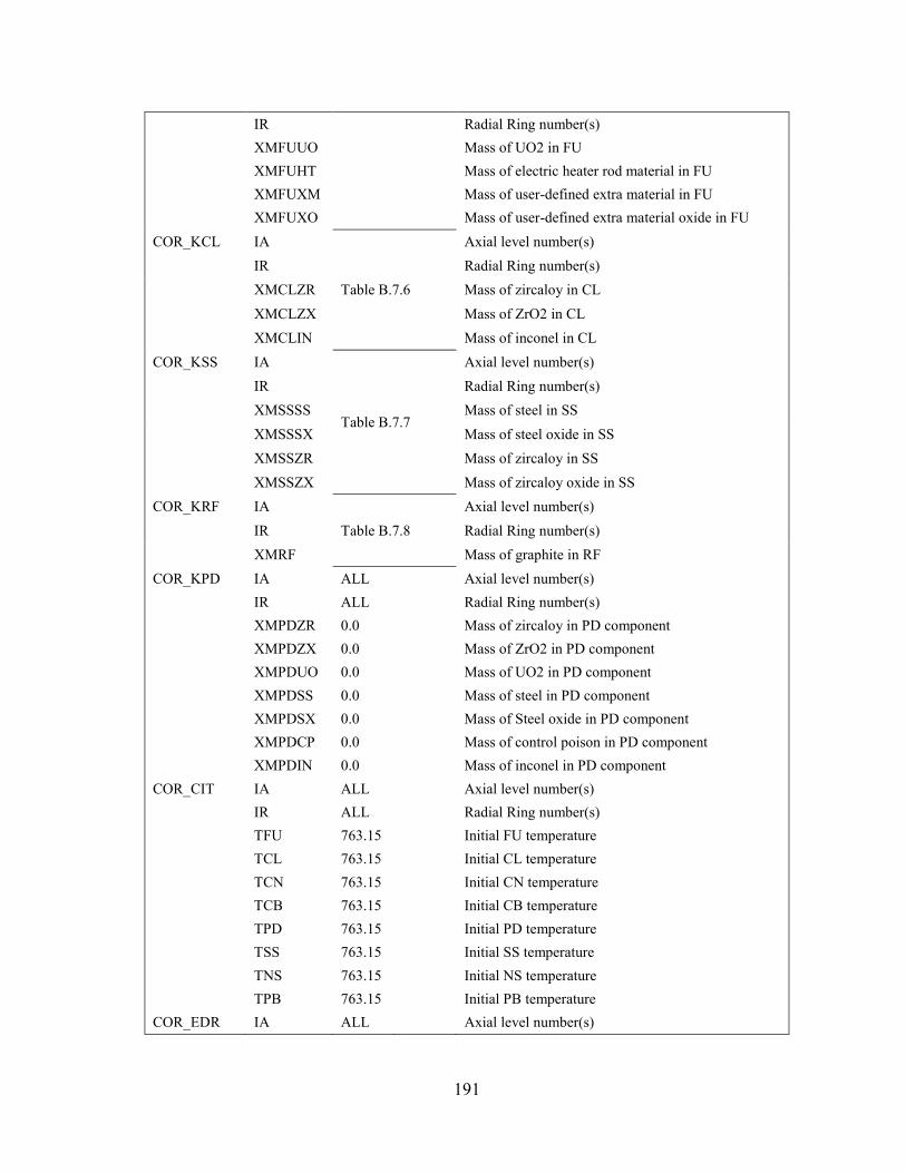
191
IR Radial Ring number(s)
XMFUUO Mass of UO2 in FU
XMFUHT Mass of electric heater rod material in FU
XMFUXM Mass of user-defined extra material in FU
XMFUXO Mass of user-defined extra material oxide in FU COR_KCL IA
Table B.7.6
Axial level number(s)
IR Radial Ring number(s)
XMCLZR Mass of zircaloy in CL
XMCLZX Mass of ZrO2 in CL
XMCLIN Mass of inconel in CL COR_KSS IA
Table B.7.7
Axial level number(s)
IR Radial Ring number(s)
XMSSSS Mass of steel in SS
XMSSSX Mass of steel oxide in SS
XMSSZR Mass of zircaloy in SS
XMSSZX Mass of zircaloy oxide in SS COR_KRF IA
Table B.7.8 Axial level number(s)
IR Radial Ring number(s)
XMRF Mass of graphite in RF COR_KPD IA ALL Axial level number(s)
IR ALL Radial Ring number(s)
XMPDZR 0.0 Mass of zircaloy in PD component
XMPDZX 0.0 Mass of ZrO2 in PD component
XMPDUO 0.0 Mass of UO2 in PD component
XMPDSS 0.0 Mass of steel in PD component
XMPDSX 0.0 Mass of Steel oxide in PD component
XMPDCP 0.0 Mass of control poison in PD component
XMPDIN 0.0 Mass of inconel in PD component COR_CIT IA ALL Axial level number(s)
IR ALL Radial Ring number(s)
TFU 763.15 Initial FU temperature
TCL 763.15 Initial CL temperature
TCN 763.15 Initial CN temperature
TCB 763.15 Initial CB temperature
TPD 763.15 Initial PD temperature
TSS 763.15 Initial SS temperature
TNS 763.15 Initial NS temperature
TPB 763.15 Initial PB temperature COR_EDR IA ALL Axial level number(s)

192
IR ALL Radial Ring number(s)
DHYCL 0.0526 CL equivalent diameter
DHYPD 0.0168 PD equivalen diameter
DHYCNC 0.0168 CNC equivalent diameter
DHYCNB 0.0168 CNB equivalent diameter
DHYSS 0.0168 SS equivalent diameter
DHYNS 0.0168 NS equivalent diameter
DHYPB 0.0168 PB equivalent diameter COR_RFD IA
Table B.7.9
Axial level number(s)
IR Radial Ring number(s)
DHYRFC RF channel side equivalent diameter
DHYRFB RF bypass side equivalent diameter COR_RFG IA
Table B.7.10
Axial level number(s)
IR Radial Ring number(s)
RADI Reflector channel-side radius
THKRF Reflector thickness
IGEOMRF Reflector geometry flag
FACRF Factor to split conductance to inner/outer surfaces COR_BFA IA
Table B.7.11
Axial level number(s)
IR Radial Ring number(s)
ASCELR Area of outer radial cell boundary = 2πR(DZ)
AFLOWC Channel flow area of cell
AFLOWB Bypass flow area of cell COR_SA IA
Table B.7.12
Axial level number(s)
IR Radial Ring number(s)
ASFU FU surface area
ASCL CL surface area
ASCN CN surface area
ASSS SS surface area
ASNS NS surface area COR_RFA IA
Table B.7.13
Axial level number(s)
IR Radial Ring number(s)
ASRF Channel-side reflector surface area
ASRFB Bypass-side reflector surface area

193
Table B.7.1
COR_SS for HTTF model
COR_SS
IA IR ISSMOD ISSFAI TSSFAI SSMETA
9 1-6 PLATEG TSFAIL 5000.0 STEEL 11 2-4 PLATEG TSFAIL 5000.0 ZIRC 22 2-4 PLATEG TSFAIL 5000.0 ZIRC 4 1-6 PLATEG TSFAIL 5000.0 STEEL 27 1-5 PLATEG TSFAIL 5000.0 STEEL 25 2-4 PLATEG TSFAIL 5000.0 ZIRC 23 2-4 PLATEG TSFAIL 5000.0 ZIRC 12 2-4 PLATEG TSFAIL 5000.0 ZIRC 8 1-6 PLATEG TSFAIL 5000.0 ZIRC 6-7 1 PLATEG TSFAIL 5000.0 ZIRC 5 1-6 PLATEG TSFAIL 5000.0 ZIRC
Table B.7.2
COR_ZP for HTTF model
COR_ZP
IA Z DZ PORDP IHSA FZPOW
1 -1.6542 0.27310 0.0 NO 0.00 2 -1.3811 0.27310 0.0 NO 0.00 3 -1.1080 0.27300 0.0 NO 0.00 4 -0.8350 0.03810 0.0 LPR_MS-04 0.00 5 -0.7969 0.07940 0.0 LPR_MS-05 0.00 6 -0.7175 0.11080 0.0 LPR_MS-06 0.00 7 -0.6067 0.11080 0.0 LPR_MS-07 0.00 8 -0.4959 0.22890 0.0 LPR_MS-08 0.00 9 -0.2670 0.02560 0.0 CB-09 0.00
10 -0.2414 0.08900 0.0 SR_CB-10 0.00 11 -0.1524 0.12700 0.0 SR_CB-11 0.00 12 -0.0254 0.02540 0.0 SR_CB-12 0.00 13 0.0000 0.19820 0.0 SR_CB-13 0.10 14 0.1982 0.19820 0.0 SR_CB-14 0.10 15 0.3964 0.19820 0.0 SR_CB-15 0.10

194
16 0.5946 0.19820 0.0 SR_CB-16 0.01 17 0.7928 0.19820 0.0 SR_CB-17 0.01 18 0.9910 0.19820 0.0 SR_CB-18 0.10 19 1.1892 0.19820 0.0 SR_CB-19 0.10 20 1.3874 0.19820 0.0 SR_CB-20 0.10 21 1.5856 0.19820 0.0 SR_CB-21 0.10 22 1.7838 0.19820 0.0 SR_CB-22 0.10 23 1.9820 0.02540 0.0 SR_CB-23 0.00 24 2.0074 0.07620 0.0 SR_CB-24 0.00 25 2.0836 0.09420 0.0 SR_CB-25 0.00 26 2.1778 0.10160 0.0 SR_CB-26 0.00 27 2.2794 0.09910 0.0 SR_CB-27 0.00
Table B.7.3
COR_RP for HTTF model
COR_RP
IR RINGR ASCELA IHSR ICFCHN ICFBYP FRPOW
1 0.1814 0.1034 CB_TOP NO NO 0.00 2 0.3116 0.2010 CB_TOP FLDIR2 NO 0.33 3 0.4015 0.2010 CB_TOP FLDIR3 NO 0.33 4 0.4748 0.2010 CB_TOP FLDIR4 NO 0.33 5 0.6030 0.4340 CB_TOP NO NO 0.00 6 0.8190 0.9650 CB_TOP NO NO 0.00
Table B.7.4
COR_RBV for HTTF model
COR_RBV
IA IR IREF JREF ICVHC ICVHB
1 1 0 0 CV001-LP CV001-LP 1 2 1 1 - - 2 1-3 1 1 - - 3 1-4 1 1 - - 1 3-5 1 1 - - 2 4-5 1 1 - -

195
3 5 1 1 - - 4-5 1-5 1 1 - - 6 1 0 0 CV106-LP CV106-LP 7 1 0 0 CV107-LP CV107-LP 6 2 0 0 CV206-LP CV206-LP 7 2 0 0 CV207-LP CV207-LP 6 3 0 0 CV306-LP CV306-LP 7 3 0 0 CV307-LP CV307-LP 6 4 0 0 CV406-LP CV406-LP 7 4 0 0 CV407-LP CV407-LP 6 5 0 0 CV506-LP CV506-LP 7 5 0 0 CV507-LP CV507-LP 8-9 1 0 0 CVCR_101 CVCR_101 10-12 1 0 0 CVCR_102 CVCR_102 13-14 1 0 0 CVCR_103 CVCR_103 15-16 1 0 0 CVCR_104 CVCR_104 17-18 1 0 0 CVCR_105 CVCR_105 19-20 1 0 0 CVCR_106 CVCR_106 21-22 1 0 0 CVCR_107 CVCR_107 23-24 1 0 0 CVCR_108 CVCR_108 25-27 1 0 0 CVCR_109 CVCR_109 8-9 2 0 0 CVCore_201 CVCore_201 10 2 0 0 CVCore_202A CVCore_202A 11-12 2 0 0 CVCore_202B CVCore_202B 13-14 2 0 0 CVCore_203 CVCore_203 15-16 2 0 0 CVCore_204 CVCore_204 17-18 2 0 0 CVCore_205 CVCore_205 19-20 2 0 0 CVCore_206 CVCore_206 21-22 2 0 0 CVCore_207 CVCore_207 23-24 2 0 0 CVCore_208 CVCore_208 25-27 2 0 0 CVCore_209 CVCore_209 8-9 3 0 0 CVCore_301 CVCore_301 10 3 0 0 CVCore_302A CVCore_302A 11-12 3 0 0 CVCore_302B CVCore_302B 13-14 3 0 0 CVCore_303 CVCore_303 15-16 3 0 0 CVCore_304 CVCore_304 17-18 3 0 0 CVCore_305 CVCore_305 19-20 3 0 0 CVCore_306 CVCore_306 21-22 3 0 0 CVCore_307 CVCore_307 23-24 3 0 0 CVCore_308 CVCore_308 25-27 3 0 0 CVCore_309 CVCore_309

196
8-9 4 0 0 CVCore_401 CVCore_401 10 4 0 0 CVCore_402A CVCore_402A 11-12 4 0 0 CVCore_402B CVCore_402B 13-14 4 0 0 CVCore_403 CVCore_403 15-16 4 0 0 CVCore_404 CVCore_404 17-18 4 0 0 CVCore_405 CVCore_405 19-20 4 0 0 CVCore_406 CVCore_406 21-22 4 0 0 CVCore_407 CVCore_407 23-24 4 0 0 CVCore_408 CVCore_408 25-27 4 0 0 CVCore_409 CVCore_409 8-9 5 0 0 CVCore_501 CVCore_501 10 5 0 0 CVCore_502A CVCore_502A 11-12 5 0 0 CVCore_502B CVCore_502B 13-14 5 0 0 CVCore_503 CVCore_503 15-16 5 0 0 CVCore_504 CVCore_504 17-18 5 0 0 CVCore_505 CVCore_505 19-20 5 0 0 CVCore_506 CVCore_506 21-22 5 0 0 CVCore_507 CVCore_507 23-24 5 0 0 CVCore_508 CVCore_508 25-27 5 0 0 CVCore_509 CVCore_509 4-27 6 NULL NULL NULL NULL 1-3 6 1 1 - -
Table B.7.5
COR_KFU for HTTF model
COR_KFU
IA IR XMFUUO XMFUHT XMFUXM XMFUXO
13-22 2 10.98 0.00 0.00 0.00 13-22 3 11.79 0.00 0.00 0.00 13-22 4 10.5742 0.00 0.00 0.00

197
Table B.7.6
COR_KCL for HTTF model
COR_KCL
IA IR XMCLZR XMCLZX XMCLIN
13-22 2.00 85.01 0.00 0.00 13-22 3.00 82.72 0.00 0.00 13-22 4.00 88.07 0.00 0.00
Table B.7.7
COR_KSS for HTTF model
COR_KSS
IA IR XMSSSS XMSSSX XMSSZR XMSSZX
25 2 0.000 0.000 7.749 0.000 25 3 0.000 0.000 8.967 0.000 25 4 0.000 0.000 4.649 0.000 23 2 0.000 0.000 12.564 0.000 23 3 0.000 0.000 12.399 0.000 23 4 0.000 0.000 12.889 0.000 12 2 0.000 0.000 12.564 0.000 12 3 0.000 0.000 12.399 0.000 12 4 0.000 0.000 12.889 0.000 8 1 0.000 0.000 69.909 0.000 8 2 0.000 0.000 115.370 0.000 8 3 0.000 0.000 117.420 0.000 8 4 0.000 0.000 113.310 0.000 8 5 0.000 0.000 289.380 0.000 6-7 1 0.000 0.000 33.839 0.000 5 1 0.000 0.000 24.249 0.000 5 2 0.000 0.000 47.149 0.000 5 3 0.000 0.000 47.149 0.000 5 4 0.000 0.000 47.149 0.000 5 5 0.000 0.000 101.810 0.000 27 1 81.240 0.000 0.000 0.000 27 2 131.570 0.000 0.000 0.000 27 3 129.860 0.000 0.000 0.000 27 4 139.180 0.000 0.000 0.000 27 5 341.060 0.000 0.000 0.000

198
9 1 20.986 0.000 0.000 0.000 9 2 34.633 0.000 0.000 0.000 9 3 35.249 0.000 0.000 0.000 9 4 34.015 0.000 0.000 0.000 9 5 86.871 0.000 0.000 0.000 4 1 31.241 0.000 0.000 0.000 4 2 60.729 0.000 0.000 0.000 4 3 60.729 0.000 0.000 0.000 4 4 60.729 0.000 0.000 0.000 4 5 131.130 0.000 0.000 0.000
Table B.7.8
COR_KRF for HTTF model
COR_KRF
IA IR XMRF
26 1 31.219 26 2 50.548 26 3 49.889 26 4 53.472 26 5 131.030 25 1 28.946 25 5 121.488 24 1 23.414 24 2 37.911 24 3 37.417 24 4 41.104 24 5 98.274 23 1 7.805 23 5 32.758 13-22 1 60.904 13-22 5 255.620 12 1 7.805 12 5 32.758 11 1 23.414 11 2 37.911 11 3 37.417 11 4 40.104 11 5 98.274

199
10 1 42.956 10 2 70.393 10 3 70.868 10 4 71.051 10 5 178.690
Table B.7.9
COR_RFD for HTTF model
COR_RFD
IA IR DHYRFC DHYRFB
10-26 1 1.00E-10 1.00E-10 24 2-4 0.0168 1.00E-10 26 2-4 0.0168 1.00E-10 11 2-4 0.0168 1.00E-10 10 2-5 0.0254 1.00E-10 11-26 5 1.00E-10 1.00E-10
Table B.7.10
COR_RFG for HTTF model
COR_RFG
IA IR RADI THKRF IGEOMRF
10-26 1 0.1814 -0.18140 1 10 2 0.3116 -0.13020 1 10 3 0.4015 -0.08990 1 10 4 0.4748 -0.07330 1 11 2 0.3116 -0.13020 1 11 3 0.4015 -0.08990 1 11 4 0.4748 -0.07330 1 24 2 0.3116 -0.13020 1 24 3 0.4015 -0.08990 1 24 4 0.4748 -0.07330 1 26 2 0.3116 -0.13020 1 26 3 0.4015 -0.08990 1 26 4 0.4748 -0.07330 1

200
Table B.7.11
COR_BFA for HTTF model
COR_BFA
IA IR ASCELR AFLOWC AFLOWB
27 1 0.1129 0.00000 0.00000 26 1 0.1158 0.00000 0.00000 25 1 0.1074 0.00000 0.00000 24 1 0.0869 0.00000 0.00000 23 1 0.0289 0.00000 0.00000 13-22 1 0.2259 0.00000 0.00000 12 1 0.0289 0.00000 0.00000 11 1 0.0869 0.00000 0.00000 10 1 0.1593 0.00000 0.00000 9 1 0.0292 0.00000 0.00000 8 1 0.2609 0.00000 0.00000 6-7 1 0.1263 0.00000 0.00000 5 1 0.0905 0.00000 0.00000 4 1 0.0434 0.00000 0.00000 3 1 0.3112 0.00000 0.00000 2 1 0.3113 0.00000 0.00000 1 1 0.311 0.00100 0.00000 27 2 0.194 0.03578 0.00000 26 2 0.1989 0.03578 0.00000 25 2 0.1844 0.03578 0.00000 24 2 0.1492 0.03578 0.00000 23 2 0.0497 0.03578 0.00000 13-22 2 0.388 0.03578 0.00000 12 2 0.0497 0.03578 0.00000 11 2 0.1448 0.03578 0.00000 10 2 0.1014 0.03040 0.00000 9 2 0.0501 0.03040 0.00000 8 2 0.4481 0.03040 0.00000 6-7 2 0.2169 0.20100 0.00000 5 2 0.1555 0.00000 0.00000 4 2 0.0746 0.00000 0.00000 3 2 0.5345 0.00000 0.00000 2 2 0.5347 0.00000 0.00000 1 2 0.5347 0.00100 0.00000 27 3 0.2499 0.03576 0.00000 26 3 0.2563 0.03576 0.00000

201
25 3 0.2376 0.03576 0.00000 24 3 0.1922 0.03576 0.00000 23 3 0.0641 0.03576 0.00000 13-22 3 0.4999 0.03576 0.00000 12 3 0.0641 0.03576 0.00000 11 3 0.1922 0.03576 0.00000 10 3 0.3527 0.02736 0.00000 9 3 0.0646 0.02736 0.00000 8 3 0.5774 0.02736 0.00000 6-7 3 0.2795 0.20100 0.00000 5 3 0.2003 0.00000 0.00000 4 3 0.0961 0.00000 0.00000 3 3 0.6887 0.00000 0.00000 2 3 0.6889 0.00000 0.00000 1 3 0.6889 0.00100 0.00000 27 4 0.2956 0.02924 0.00000 26 4 0.3031 0.02924 0.00000 25 4 0.281 0.02924 0.00000 24 4 0.2273 0.02924 0.00000 23 4 0.0758 0.02924 0.00000 13-22 4 0.5913 0.02924 0.00000 12 4 0.0758 0.02924 0.00000 11 4 0.2273 0.02924 0.00000 10 4 0.4171 0.03344 0.00000 9 4 0.0764 0.03344 0.00000 8 4 0.6829 0.03344 0.00000 6-7 4 0.3305 0.20100 0.00000 5 4 0.2369 0.00000 0.00000 4 4 0.1137 0.00000 0.00000 3 4 0.8144 0.00000 0.00000 2 4 0.8147 0.00000 0.00000 1 4 0.8147 0.00100 0.00000 27 5 0.3755 0.00000 0.00000 26 5 0.3849 0.00000 0.00000 25 5 0.3569 0.00000 0.00000 24 5 0.2887 0.00000 0.00000 23 5 0.0962 0.00000 0.00000 13-22 5 0.7509 0.00000 0.00000 12 5 0.0962 0.00000 0.00000 11 5 0.2887 0.00000 0.00000 10 5 0.5297 0.00608 0.00000

202
9 5 0.0969 0.00608 0.00000 8 5 0.8672 0.00608 0.00000 6-7 5 0.4198 0.43400 0.00000 5 5 0.3008 0.00000 0.00000 4 5 0.1444 0.00000 0.00000 3 5 1.0343 0.00000 0.00000 2 5 1.0347 0.00000 0.00000 1 5 1.0347 1.00E-03 0.00000 3 6 1.4048 1.00E-03 0.00000 2 6 1.4054 1.00E-03 0.00000 1 6 1.4054 1.00E-03 0.00000
Table B.7.12
COR_SA for HTTF model
COR_SA
IA IR ASFU ASCL ASCN ASSS ASNS
1-3 1-2 0.00 0.00 0.00 0.00 0.00 2-3 3 0.00 0.00 0.00 0.00 0.00 3 4 0.00 0.00 0.00 0.00 0.00 4 1 0.00 0.00 0.00 0.04 0.00 4 2-4 0.00 0.00 0.00 0.20 0.00 4 5 0.00 0.00 0.00 4.34E-01 0.00 4 6 0.00 0.00 0.00 0.96 0.00 5 1 0.00 0.00 0.00 0.09 0.00 5 2-4 0.00 0.00 0.00 0.20 0.00 5 5 0.00 0.00 0.00 0.43 0.00 6 1 0.00 0.00 0.00 1.26E-01 0.00 6 2-5 0.00 0.00 0.00 0.00 0.00 7 1 0.00 0.00 0.00 0.13 0.00 7 2-5 0.00 0.00 0.00 0.00 0.00 8 1 0.00 0.00 0.00 0.26 0.00 8 2 0.00 0.00 0.00 1.27 0.00 8 3 0.00 0.00 0.00 1.16 0.00 8 4 0.00 0.00 0.00 1.37 0.00 8 5 0.00 0.00 0.00 0.65 0.00 9 1 0.00 0.00 0.00 2.92E-02 0.00 9 2 0.00 0.00 0.00 0.12 0.00 9 3 0.00 0.00 0.00 0.11 0.00

203
9 4 0.00 0.00 0.00 0.13 0.00 9 5 0.00 0.00 0.00 0.02 0.00 10 1 0.00 0.00 0.00 0.00 0.00 11 1 0.00 0.00 0.00 0.00 0.00 12 1 0.00 0.00 0.00 0.00 0.00 13-22 1 0.00 0.00 0.00 0.00 0.00 23 1 0.00 0.00 0.00 0.00 0.00 24 1 0.00 0.00 0.00 0.00 0.00 25 1 0.00 0.00 0.00 0.00 0.00 26 1 0.00 0.00 0.00 0.00 0.00 27 1 0.00 0.00 0.00 0.11 0.00 10 2 0.00 0.00 0.00 0.00 0.00 11 2 0.00 0.00 0.00 0.00 0.00 12 2 0.00 0.00 0.00 0.00 0.00 13-22 2 0.96 1.65 0.00 0.00 0.00 23 2 0.00 0.00 0.00 0.00 0.00 24 2 0.00 0.00 0.00 0.00 0.00 25 2 0.00 0.00 0.00 0.00 0.00 26 2 0.00 0.00 0.00 0.00 0.00 27 2 0.00 0.00 0.00 0.00 0.00 10 3 0.00 0.00 0.00 0.00 0.00 11 3 0.00 0.00 0.00 0.00 0.00 12 3 0.00 0.00 0.00 0.00 0.00 13-22 3 1.03 1.69 0.00 0.00 0.00 23 3 0.00 0.00 0.00 0.00 0.00 24 3 0.00 0.00 0.00 0.00 0.00 25 3 0.00 0.00 0.00 0.00 0.00 26 3 0.00 0.00 0.00 0.00 0.00 27 3 0.00 0.00 0.00 0.00 0.00 10 4 0.00 0.00 0.00 0.00 0.00 11 4 0.00 0.00 0.00 0.00 0.00 12 4 0.00 0.00 0.00 0.00 0.00 13-22 4 0.93 1.23 0.00 0.00 0.00 23 4 0.00 0.00 0.00 0.00 0.00 24 4 0.00 0.00 0.00 0.00 0.00 25 4 0.00 0.00 0.00 0.00 0.00 26 4 0.00 0.00 0.00 0.00 0.00 27 4 0.00 0.00 0.00 0.00 0.00 10 5 0.00 0.00 0.00 0.00 0.00 11 5 0.00 0.00 0.00 0.00 0.00 12 5 0.00 0.00 0.00 0.00 0.00

204
13-22 5 0.00 0.00 0.00 0.00 0.00 23 5 0.00 0.00 0.00 0.00 0.00 24 5 0.00 0.00 0.00 0.00 0.00 25 5 0.00 0.00 0.00 0.00 0.00 26 5 0.00 0.00 0.00 0.00 0.00
Table B.7.13
COR_RFA for HTTF model
COR_RFA
IA IR ASRF ASRFB
10 1 1.59E-01 0.0000 11 1 8.68E-02 0.0000 12 1 2.90E-02 0.0000 13-22 1 2.26E-01 0.0000 23 1 2.90E-02 0.0000 24 1 8.69E-02 0.0000 25 1 1.07E-01 0.0000 26 1 1.16E-01 0.0000 10 2 4.26E-01 0.0000 11 2 1.00E+00 0.0000 24 2 1.06E+00 0.0000 26 2 1.05E+00 0.0000 10 3 3.84E-01 0.0000 11 3 1.08E+00 0.0000 24 3 0.6501 0.0000 26 3 0.8668 0.0000 10 4 0.4687 0.0000 11 4 0.5618 0.0000 24 4 0.6987 0.0000 26 4 0.7443 0.0000 10 5 0.4171 5.30E-01 11 5 0.2273 2.89E-01 12 5 0.0758 9.62E-02 13-22 5 0.5913 7.51E-01 23 5 0.0758 9.62E-02 24 5 0.2273 2.89E-01 25 5 2.81E-01 0.3569 26 5 3.03E-01 0.3849

205
Table B.8
MP input for HTTF model
MP_INPUT - - Signal start of MP input MP_ID MATNAM
Table B.8.1
Material name MP_PRTF PROP Property Mnemonic (ENH, CPS, THC, or RHO)
ITBPRP Name of TF for property
CFKEY CF/TF flag MP_PRC RHOM Material density (constant property)
TMLT Material melt temperature (constant property)
LHF Material latent heat of fusion (constant property)
Table B.8.1
MP properties input for HTTF model
MP_ID MP_PRTF MP_PRC
MATNAM PROP ITBPRP KEY RHOM TMLT LHF
GRAPHITE THC THC-COR_GRAPH TF 2971.6 3866.0 - CPS CPS-COR_GRAPH TF
ENH ENH-GRAPH TF STAINLESS-STEEL-304 - - - - - - ZIRCALOY THC THC-SRLP_GRAPH TF
2954.6 3866.0 - CPS CPS-SRLP_GRAPH TF
ENH ENH-GRAPH TF ZIRCONIUM-OXIDE - - - - - - STAINLESS-STEEL - - - - - - ALUMINUM THC THC-SRLP_GRAPH TF
2954.6 3866.0 - CPS CPS-SRLP_GRAPH TF
ENH ENH-GRAPH TF ALUMINUM-OXIDE - - - - - - CARBON-STEEL - - - - - - BORON-CARBIDE - - - - - - URANIUM-DIOXIDE THC THC-SiC TF
2400.0 3003.0 CPS CPS-SiC TF INCONEL THC THC-COR_GRAPH TF
2971.6 3866.0 - CPS CPS-COR_GRAPH TF
ENH ENH-GRAPH TF

206
Table B.9
TF input for HTTF model
TF_INPUT - - Signal start of TF input TF_ID TFNAME
Table B.9.1
Tabular function name
TFSCAL Tabular function scalar applied to each data point
TFADCN Tabular function additive constant applied to each data point TF_TAB NPAR Data pair number
X Independent variable (e.g. time or temperature)
Y Dependent variable
Table B.9.1
TF tabular data for HTTF model
TF_ID TF_TAB
TFNAME TFSCAL TFADCN NPAR X Y
THC-COR_GRAPH 1 0 1 25.0 4.1000
2 400.0 3.9000
3 985.0 3.4000
4 1315.0 5.0000
5 1800.0 6.5000 CPS-COR_GRAPH 1 0 1 25.0 428.000
2 400.0 849.000
3 985.0 1078.000
4 1315.0 1131.000
5 1800.0 1173.000 ENH-GRAPH 1 0 1 300.0 0.0
2 773.0 547910.0
3 1273.0 1414010.0
4 1773.0 2381110.0
5 2273.0 3405060.0
6 2773.0 4464560.0
7 3866.0 6879781.0
8 3866.0 8879871.0
9 5000.0 9456545.0 THC-SRLP_GRAPH 1 0 1 25.0 1.9
2 370.0 1.8
3 925.0 1.6
4 1130.0 2.1

207
5 1320.0 3.6 CPS-SRLP_GRAPH 1 0 1 25.0 451.0
2 370.0 876.0
3 925.0 1113.0
4 1130.0 1149.0
5 1320.0 1175.0 THC-SiC 1 0 1 273.2 340.0
2 5000.0 340.0 CPS-SiC 1 0 1 273.2 0.16
2 5000.0 0.35
Table B.10
CF input for HTTF model
CF_INPUT - - Signal start of CF input CF_ID CFNAME
Table B.10.1
Control function name
CFTYPE Control function type CF_SAI CFSCAL Control function value scalar
CFADCN Control function value additive constant
CFVALR Control function initial value CF_ARG CHARG Control function argument identifier
ARSCAL Control function argument scalar
ARADCN Control function argument additive constant

208
Table B.10.1
CF arguments for HTTF model
CF_ID CF_SAI CF_ARG
CFNAME ICFNUM CFTYP CFSCAL CFADCB CFVALR CHARG ARSCAL ARADCN
RCCS-T-0 700 EQUALS 0.0 300.00 300.00 EXEC-TIME 0.00 0.00 RCCS-T-7 707 EQUALS 0.0 300.00 300.00 EXEC-TIME 0.00 0.00
Trans-T0 1 EQUALS 0.0 0.00 0.00 EXEC-TIME 0.00 0.00 Trans-dt 2 ADD 0.0 0.00 0.00 EXEC-TIME 1.00 0.00
CF-VALU('Trans-T0') -1.00 0.00 Trans-Trip-Time 3 EQUALS 0.0 0.00 0.00 EXEC-TIME 0.00 0.00 Trans-Trip 4 L-GT - - - CF-VALU('Trans-dt') 1.00 0.00
CF-VALU('Trans-Trip-Time') 1.00 0.00 SS-Mflow 50 EQUALS 0.0 0.96 0.96 EXEC-TIME 0.00 0.00 HeVelocity 51 DIVIDE 1.0 0.00 0.00 CVH-RHO('CV160-Gap',HE) 0.08 0.00
CF-VALU('SS-Mflow') 1.00 0.00 HeSource 52 L-A-IFTE 1.0 0.00 0.00 CF-VALU('Trans-Trip') - -
EXEC-TIME 0.00 0.00
CF-VALU('HeVelocity') 1.00 0.00 SS-Pin 53 EQUALS 0.0 8.00E+05 8.00E+05 EXEC-TIME 0.00 0.00 Trans-Pin 54 EQUALS 0.0 1.00E+05 1.00E+05 EXEC-TIME 0.00 0.00 SourceP 55 L-A-IFTE 1.0 0.00 8.00E+05 CF-VALU('Trans-Trip') - -
CF-VALU('Trans-Pin') 1.00 0.00
CF-VALU('SS-Pin') 1.00 0.00 SS-Pout 56 EQUALS 0.0 8.00E+05 8.00E+05 EXEC-TIME 0.00 0.00 Trans-Pout 57 EQUALS 0.0 1.00E+05 1.00E+05 EXEC-TIME 0.00 0.00

209
SinkP 58 L-A-IFTE 1.0 0.00 8.00E+05 CF-VALU('Trans-Trip') - - CF-VALU('Trans-Pout') 1.00 0.00
CF-VALU('SS-Pout') 1.00 0.00 SS-Tin 59 EQUALS 0.0 532.15 532.15 EXEC-TIME 0.00 0.00 Trans-Tin 60 EQUALS 0.0 300.00 300.00 EXEC-TIME 0.00 0.00 SourceT 61 L-A-IFTE 1.0 0.00 532.15 CF-VALU('Trans-Trip') - -
CF-VALU('Trans-Tin') 1.00 0.00
CF-VALU('SS-Tin') 1.00 0.00 SS-Tout 62 EQUALS 0.0 960.15 960.15 EXEC-TIME 0.00 0.00 Trans-Tout 63 EQUALS 0.0 300.00 300.00 EXEC-TIME 0.00 0.00 SinkT 64 L-A-IFTE 1.0 0.00 960.15 CF-VALU('Trans-Trip') - -
CF-VALU('Trans-Tout') 1.00 0.00
CF-VALU('SS-Tout') 1.00 0.00 Humidity 65 EQUALS 0.0 0.00 0.00 EXEC-TIME 0.00 0.00 Src_HeFrac 66 EQUALS 0.0 1.00 1.00 EXEC-TIME 0.00 0.00 Sink_N2-Frac 67 EQUALS 0.0 0.80 0.80 EXEC-TIME 0.00 0.00 Sink_02-Frac 68 EQUALS 0.0 0.20 0.20 EXEC-TIME 0.00 0.00 InletVlv 69 L-A-IFTE 1.0 0.00 1.00 CF-VALU('Trans-Trip') - -
EXEC-TIME 0.00 0.00
EXEC-TIME 0.00 1.00 EmisCB 80 EQUALS 0.0 0.21 0.21 EXEC-TIME 0.00 0.00 EmisVes 81 EQUALS 0.0 0.21 0.21 EXEC-TIME 0.00 0.00 EmisRCCS 82 EQUALS 0.0 0.21 0.21 EXEC-TIME 0.00 0.00 CORE-POWER 100 EQUALS 0.0 2.20E+06 2.20E+06 EXEC-TIME 0.00 0.00 FLDIR2 102 EQUALS 1.0 0.0 0.0 FL-VEL('FL_209to208','A') -1.00 0.00 FLDIR3 103 EQUALS 1.0 0.0 0.0 FL-VEL('FL_309to308','A') -1.00 0.00 FLDIR4 104 EQUALS 1.0 0.0 0.0 FL-VEL('FL_409to408','A') -1.00 0.00

210
Table B.11
EXEC MELCOR input for HTTF model
EXEC_TEND TEND 0.0 Calculation end time EXEC_TIME TIME -1000.0 Time
DTMAX 0.5 Maximum time-step
DTMIN 1.00E-05 Minimum time-step
DTEDIT 500.0 Frequency of edit printing
DTPLOT 1.0 Frequency of plot file writing
DTREST 1000.0 Restart frequency
DCREST 1.00E+10 Restart frequency with respect to CPU time
EXEC_CPULEFT CPULEF 30.0 Desired minimum number of CPU seconds left at end of calculation
EXEC_CPULIM CPULIM 1200.0 Maximum number of CPU seconds for the calculation
EXEC_CYMESF NCYEDD 100 Number of cycles between messages written to
terminal
NCYEDP 1000 Number of cycles between messages to output file EXEC_EXACTTIME N 1 Data string index
TIME 0 Desired time to land on exactly during calculation