Thermal effects of fluid flowin the Colorado Plateau and the Grand Canyon

Georg-August-University GottingenFaculty of Geosciences and Geography

Department of Structural Geology and Geodynamics

Master’s thesis

submitted in Partial Fulfillmentof the Requirements for the Degree of

Master of Science (M.Sc.)in Geoscience

by

Axel Ludersborn on the 18.07.1990 in Hamburg

9. February 2018

Supervisor: Dr. Elco Luijendijk, Dept. of Structural Geology and Geodynamics,Georg-August-University Gottingen, Gottingen, Germany

Co-supervisor: Dr. Matthew Fox, Dept. of Earth Sciences, University College London,London, England

Declaration

Hiermit versichere ich, dass ich die vorliegende Masterarbeit selbstandig und nur mit denangegebenen Hilfsmitteln verfasst habe. Alle Passagen, die ich wortlich oder sinngemaßaus der Literatur oder aus anderen Quellen wie z.B. Internetseiten ubernommen habe,habe ich deutlich als Zitat mit Angabe der Quelle kenntlich gemacht. Daruber hinausversichere ich, dass die eingereichte Arbeit weder vollstandig noch in wesentlichen TeilenGegenstand eines anderen Prufungsverfahrens gewesen ist. Eine gegebenenfalls eingere-ichte digitale Version stimmt mit der schriftlichen Fassung uberein.

Datum: Unterschrift:

Acknowledgment

In the first place, i am more than grateful of my two supervisors Dr. Elco Luijendijk andDr. Matthew Fox for providing me the opportunity to carry out this interesting study ofnumerical modeling of groundwater and heat flow in the Grand Canyon.Special thanks to supervisor Dr. Elco Luijendijk for introducing me to the modeling withSutra. Your patience, positive, humorful and motivating way plus your valueable feed-back throughout the entire master thesis time helped me a lot. Also, I can’t express howgrateful I am that you always have an open door for my concerns.I would also like to express my gratitude to Pascal and Mogens for their friendship, scien-tific exchange, correction of my master thesis and their support in all matters. Thanks tomy office mate Torben for the nice and amusing time. Another thanks goes to Sarah forthe correction of my master thesis and useful improvements on my english writing. Phudeserves a special thanks for checking my LaTeX file and having some awesome meals.And last but not least, I would like to thank my family for their unconditional supportand encouragements in this special time.

Abstract

The timing of the formation of the Grand Canyon is still not fully understood, especially1) whether the Grand Canyon is most recently carved by the Colorado River at 5-6 Maago or 2) the Grand Canyon has been formed 70 - 55 Ma ago. Extensive thermochrono-logical measurements could not provide unambiguous age control. The interpretation ofthermochronological data depends on geothermal gradients, which can be influenced bygroundwater flow. Therefore, information on groundwater and heat flow could provideimportant constraints on the thermal history of the Grand Canyon. In this thesis I use2-D numerical model of groundwater and heat flow to infer past and present-day temper-ature geothermal gradients of the Grand Canyon. I calibrated the model permeabilitiesusing hydrogeological datasets like groundwater recharge and spring discharge.The results show varying geothermal gradients in time and space. Present-day condi-tions demonstrate higher geothermal gradients in the area of the Colorado River (∼ 28◦C)whereas the areas at higher altitudes show lower geothermal gradients (∼ 10◦C) due tocooling effect of groundwater flow. Due to the upwards flow, the area close to the Col-orado River is being heated up by ∼ 14◦C while the largest part of the model is beingcooled down up to 32◦C. Moreover, this cooling effect increases with higher groundwaterrecharge values in the Pleistocene. The results indicate that groundwater flow and heatflow data alter the thermal history of the Grand Canyon and therefore should be includedin interpretations of the time of formation that rely on low-temperature thermochronology.

I Contents

Contents

Declaration . . . . . . . . . . . . . . . . . . . . . . . . . . . . . . . . . . . . . . . IAcknowledgment . . . . . . . . . . . . . . . . . . . . . . . . . . . . . . . . . . . . IIAbstract . . . . . . . . . . . . . . . . . . . . . . . . . . . . . . . . . . . . . . . . . III

1 Introduction 1

2 Study Area 32.1 Stratigraphy and Lithology . . . . . . . . . . . . . . . . . . . . . . . . . . . 32.2 Hydrogeology . . . . . . . . . . . . . . . . . . . . . . . . . . . . . . . . . . . 5

3 Methods 63.1 Groundwater recharge and spring water budget . . . . . . . . . . . . . . . . 63.2 Groundwater and heat flow model . . . . . . . . . . . . . . . . . . . . . . . 7

3.2.1 Groundwater and heat flow model equations . . . . . . . . . . . . . 73.2.2 Permeabilites of lithologic units . . . . . . . . . . . . . . . . . . . . . 93.2.3 Model boundaries and initial conditions . . . . . . . . . . . . . . . . 10

3.2.3.1 Groundwater recharge . . . . . . . . . . . . . . . . . . . . . 103.2.4 Model discretization . . . . . . . . . . . . . . . . . . . . . . . . . . . 113.2.5 Model calibration . . . . . . . . . . . . . . . . . . . . . . . . . . . . . 113.2.6 Groundwater flow in the Pleistocene . . . . . . . . . . . . . . . . . . 12

4 Results 134.1 Spring water budget . . . . . . . . . . . . . . . . . . . . . . . . . . . . . . . 134.2 Simulations for the model calibration . . . . . . . . . . . . . . . . . . . . . . 144.3 Groundwater flow in the Pleistocene . . . . . . . . . . . . . . . . . . . . . . 21

5 Discussion 24

6 Conclusion 26

7 Appendix IAppendix . . . . . . . . . . . . . . . . . . . . . . . . . . . . . . . . . . . . . . . . I

II List of Figures

List of Figures

1.1 Regional geography and topography of the Grand Canyon along the Col-orado River as a part of the Colorado Plateau located in the southwesternUnited States of America. The dotted line demonstrates the restricted areaof the study area whereas the line A - A’ indicates a cross section. Whitedots mark the location of springs. . . . . . . . . . . . . . . . . . . . . . . . . 2

2.1 Generalized stratigraphic section of the Grand Canyon demonstrating theapproximated thickness of the respective layers, water bearing units, theregional Redwall-Muav Aquifer. Modified after Beus and Morales (2003). . 4

3.1 Map showing the watersheds of the study area in the Grand Canyon. Thearea is divided into two parts. The northern area (purple color) representsthe higher altitude, whereas the the southern area (brown color) correspondsto the lower altitudes. The National Elevation Dataset(NED) is a rasterprodcut assembled by USGS (2013). Watershed and high relief data areprovided by USGS as well. . . . . . . . . . . . . . . . . . . . . . . . . . . . . 6

3.2 Sketch showing the model setup and the adjacent boundary conditions thatare present along the identified cross-section. . . . . . . . . . . . . . . . . . 9

3.3 Model domain contains stratigraphic units in simplified vertical extent andmentioned horizontal lines which divide the rectangles. Not included arethe element outlines. . . . . . . . . . . . . . . . . . . . . . . . . . . . . . . . 11

4.1 Best-calibrated model simulation for the 2D-cross-section from the studyarea, showing the temperature profile with groundwater recharge conditionsat present-day. The flow vectors indicate the groundwater flow directions. . 14

4.2 Comparison of temperature-depth relations in the model at position (a) x= 0 m and (b) x = 23490 m. . . . . . . . . . . . . . . . . . . . . . . . . . . 15

4.3 Section of the discharge area with locations of the Colorado River (1) andthe Dragon spring (2). Best-calibrated model simulation showing the tem-perature profile with groundwater recharge conditions at present-day andflow vectors for the groundwater flow direction. . . . . . . . . . . . . . . . . 16

III List of Figures

4.4 The relation between discharge of the Dragon Spring and the Colorado Riverto Permeability for specific lithologic units (a) Redwall-Muav-Aquifer, (b)Bright Angle Shale, (c) Early Proterozoic Sedimentary Rocks and (d) Mid-dle Proterozoic Sedimentary Rocks. The Permeability is plotted on thex-axis and the discharge is plotted on the y-axis. The blue dots, which areconnected with lines, show calculated discharge values of several perme-ability settings for the Dragon spring, whereas the red dots represent theColorado River. . . . . . . . . . . . . . . . . . . . . . . . . . . . . . . . . . . 16

4.5 Modeled temperature trend for groundwater recharge scenario = 0 mm yr−1. 174.6 Showing the temperature difference of a groundwater recharge scenario

(41.3 mm yr−1) versus a non-groundwater recharge (0 mm yr−1) scenarioin depth. Graph (a) represents a depth-profile for position x = 0 and (b)for position x = 23490 m. . . . . . . . . . . . . . . . . . . . . . . . . . . . . 17

4.7 Two different rock properties, which are applied in each scenario to everylithological unit. The shown temperature profiles demonstrate the differ-ence between rock properties for the porosity of (a) = 5% and (b) = 25%.Flow vectors demonstrate the groundwater flow directions. . . . . . . . . . . 18

4.8 Two different rock properties, which are applied in each scenario to everylithological unit. The shown temperature profiles demonstrate the differ-ence between rock properties for the thermal conductivity of the rock ma-trix (a) = 1.5 and (b) = 4. Flow vectors demonstrate the groundwater flowdirections. . . . . . . . . . . . . . . . . . . . . . . . . . . . . . . . . . . . . . 18

4.9 Two hydraulic head versus depth plots, showing the potential energy of thewater for positions of (a) x = 0 m and (b) x = 23490 m in the model domain. 19

4.10 Velocity-Depth relationship for position (a) x = 0 m and (b) x = 23490 inthe model domain. Graph (a) shows increasing velocities towards the uppermodel domain, whereas the graph (b) slows down towards the bottom modeldomain. . . . . . . . . . . . . . . . . . . . . . . . . . . . . . . . . . . . . . . 20

4.11 Modeled groundwater recharge scenarios versus average temperature usingtemperature profile at position x = 23490 m. Horizontal lines are showingthe estimated values for present-day (1) and Pleistocene (2) groundwaterrecharge scenarios. . . . . . . . . . . . . . . . . . . . . . . . . . . . . . . . . 21

4.12 Modeled groundwater flow and temperature trends for groundwater rechargescenarios of (a) 20 mm yr−1, (b) 40 mm yr−1 and (c) 80 mm yr−1. Flowvectors demonstrate the groundwater flow directions. . . . . . . . . . . . . . 22

4.13 Modeled groundwater flow and temperature trends for groundwater rechargescenarios of (d) 120 mm yr−1, (e) 160 mm yr−1 and (f) 200 mm yr−1. Sce-nario (d) and (e) represent the groundwater flow in the Pleistocene (Zhuet al., 2003). Flow vectors demonstrate the groundwater flow directions. . . 23

IV List of Tables

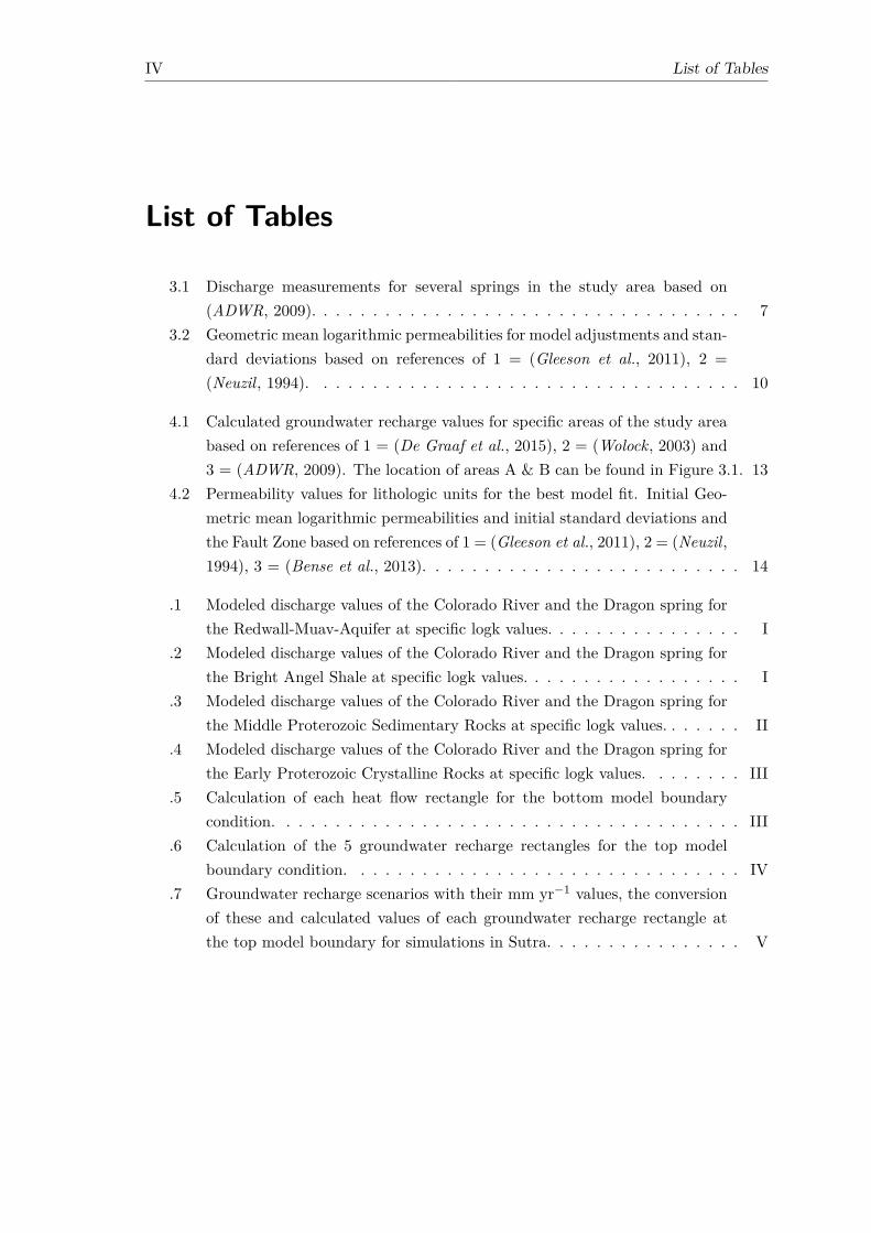
List of Tables

3.1 Discharge measurements for several springs in the study area based on(ADWR, 2009). . . . . . . . . . . . . . . . . . . . . . . . . . . . . . . . . . . 7

3.2 Geometric mean logarithmic permeabilities for model adjustments and stan-dard deviations based on references of 1 = (Gleeson et al., 2011), 2 =(Neuzil, 1994). . . . . . . . . . . . . . . . . . . . . . . . . . . . . . . . . . . 10

4.1 Calculated groundwater recharge values for specific areas of the study areabased on references of 1 = (De Graaf et al., 2015), 2 = (Wolock, 2003) and3 = (ADWR, 2009). The location of areas A & B can be found in Figure 3.1. 13

4.2 Permeability values for lithologic units for the best model fit. Initial Geo-metric mean logarithmic permeabilities and initial standard deviations andthe Fault Zone based on references of 1 = (Gleeson et al., 2011), 2 = (Neuzil,1994), 3 = (Bense et al., 2013). . . . . . . . . . . . . . . . . . . . . . . . . . 14

.1 Modeled discharge values of the Colorado River and the Dragon spring forthe Redwall-Muav-Aquifer at specific logk values. . . . . . . . . . . . . . . . I

.2 Modeled discharge values of the Colorado River and the Dragon spring forthe Bright Angel Shale at specific logk values. . . . . . . . . . . . . . . . . . I

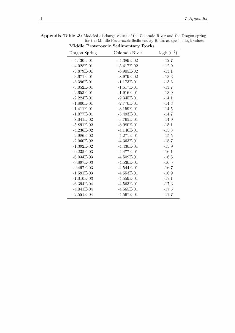
.3 Modeled discharge values of the Colorado River and the Dragon spring forthe Middle Proterozoic Sedimentary Rocks at specific logk values. . . . . . . II

.4 Modeled discharge values of the Colorado River and the Dragon spring forthe Early Proterozoic Crystalline Rocks at specific logk values. . . . . . . . III

.5 Calculation of each heat flow rectangle for the bottom model boundarycondition. . . . . . . . . . . . . . . . . . . . . . . . . . . . . . . . . . . . . . III

.6 Calculation of the 5 groundwater recharge rectangles for the top modelboundary condition. . . . . . . . . . . . . . . . . . . . . . . . . . . . . . . . IV

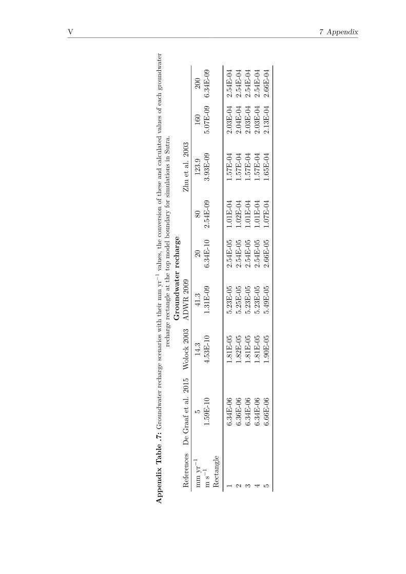
.7 Groundwater recharge scenarios with their mm yr−1 values, the conversionof these and calculated values of each groundwater recharge rectangle atthe top model boundary for simulations in Sutra. . . . . . . . . . . . . . . . V

1 1 Introduction

1 Introduction

What is known about the timing of formation of the Grand Canyon is based on numer-ous studies which have been vigorously debated over nearly a century (Karlstrom et al.,2014). All these theories (whether the oldest or youngest) rely almost exclusively on ther-mochronological data. Thermochronology methods like apatite fission-track (AFT) dataand (U-Th)/He systems can be used to derive the temperature history of specific rocks.Both methods show overlaps for cooling constraints for ranges of temperature. Literaturereveal temperatures for AFT at 60 - 110 ◦C (Ketcham et al., 2007),while the temperaturefor (U-Th)/He (AHe) dating is classified between 30 - 90 ◦C (Farley, 2000; Shuster andFarley, 2004). These temperatures give evidence for the thermal history of the rock whichcan be derived by means of exhumation. Moreover, the burial depth can be linked tothose temperatures. Nevertheless, there has been some disagreement in thermochronolog-ical measurements regarding the time of formation of the Grand Canyon. Previous findingshave led to a huge gap in the timescale. Several studies underpin the ”old“ canyon model,but then again a lot of recent researches suggests the ”young“ canyon model to be accu-rate. According to Wernicke (2011) the former model state that the most of the GrandCanyon was formed by precursor rivers, beginning the process of incision at 80 - 70 Mayears ago, whereas the second one reflects that the Grand Canyon was carved throughintegration of paleocanyons prior to 6 - 5 Ma years (Karlstrom et al., 2008). For precisecooling times and the associated incision of the Canyon more impact factors should beestablished to quantify the correct geothermal gradients. One of those impact factorsmight be the groundwater and heat flow. It is known that the subsurface temperaturecan change due groundwater flow (Irvine et al., 2015; Anderson, 2005; Keshari and Koo,2007). According to Hill et al. (2016) the groundwater flow does affect the interpretationsof thermochronology. Therefore, it is necessary to gain better insights by means of ther-mal effects of groundwater and heat flow to obtain geothermal gradients for the GrandCanyon.The thermal effect is governed by lots of interactions and strongly underlies the permeabil-ity of the lithologies (Gleeson et al., 2011). Permeability is decisive for the quantificationof groundwater fluxes but varies by more than 13 orders of magnitude and is difficult todetermine (Gleeson et al., 2011). Moreover, the heterogeneity, faults and joints in lay-ers in the Grand Canyon constrain the quantification of the permeability. Consequently,the uncertainty of permeability requires a closer inspection of subsurface temperatures ofgroundwater to classify thermal effects and the related geothermal gradients.

2 1 Introduction

In this study, I use a two-dimensional groundwater and heat flow model (Sutra, version 3.9)along a determined cross-section (Figure 1.1) in the Grand Canyon to quantify present andpast fluid flow and its influence on subsurface temperatures. This model aims to improvethe knowledge of thermal effects of groundwater and heat flow in the study area.

Figure 1.1: Regional geography and topography of the Grand Canyon along the Colorado Riveras a part of the Colorado Plateau located in the southwestern United States ofAmerica. The dotted line demonstrates the restricted area of the study area whereasthe line A - A’ indicates a cross section. White dots mark the location of springs.

3 2 Study Area

2 Study Area

2.1 Stratigraphy and Lithology

The Grand Canyon is one of the biggest erosional features in the world. It is located inthe northwest of Arizona and partly belongs to the Colorado Plateau. The area aroundthe Canyon is subdivided into different parts: The Kanab, Kaibab, Unikaret, ShivwitsPlateau in the north and the Hualapei and Coconino part in the south (Ingraham et al.,2001). The study area is located in the Kanab Plateau as shown in Figure 1.1. On aver-age the Grand Canyon is 13 - 16 km wide and more than 1.6 km deep. The steep sidedcanyon is carved by the Colorado River and exposes stratigraphic sections of Proterozoicand Paleozoic age. However, the geological record from the Ordovician, Silurian, Meso-zoic and Cenozoic are missing (Foos, 1999). According to Metzger (1961), the basementconsists of Vishnu Rocks, the oldest rocks in that area, which are intruded by dikes andhave been metamorphosed from igneous rocks into gneiss, whereas the overlaying GrandCanyon series consits of deposited sea sediments. The Great Unconformity above theGrand Canyon series separates the Proterozoic from the Paleozoic units. The Paleozoicstrata begins from here on and demonstrates a transition from near shore to offshore en-vironments corresponding to transgression which takes place due the global sea-level rise(Foos, 1999). The first depositional event includes the units of the Tapeats Sandstone, theBright Angel Shale and the Muav Limestone that are shown in a Figure 2.1. After periodsof lower sea-levels, the marine unit of the Redwall Limestone marks a sea level rise. Atthe end of the Mississipian age a karst landscape developed. The following unit in thesection is the Supai Group which can be dated to the Pennsylvanian and Permian. Thesediments are typical for a delta to near shore beach environment. Overlain is the HermitFormation which shows deposits of a broad coastal plain (Price, 1999). Above this layerthe Coconino Sandstone with eolian deposits is exposed. The both remaining units, theToroweap Formation and Kaibab limestone, represent marine units.Partly exposed in the section of the Grand Canyon are the Triassic sedimentary rockthat are subdivided into the Moenkopi formation and the Shinarump formation. For acloser and a more detailed view Figure 2.1 shows the segmentation of layers, the ages andthickness of the respective layers as well as the material compositions.

4 2 Study Area

Figure 2.1: Generalized stratigraphic section of the Grand Canyon demonstrating the approxi-mated thickness of the respective layers, water bearing units, the regional Redwall-Muav Aquifer. Modified after Beus and Morales (2003).

5 2 Study Area

2.2 Hydrogeology

According to Hill and Polyak (2010), the Mississippian Redwall Limestone and the Cam-brian Muav Limestone should be highlighted because of their excellent reservoir qualityfor storing large quantities of water. Both hydro-stratigraphic units can be comprised intoone main karstic horizon which is the Redwall-Muav aquifer. Nevertheless, the Coconinolimestone can also be seen as a smaller water-bearing unit, which allows the downwardspercolation of groundwater (Metzger , 1961).The groundwater flow starts at the surface and descends through fractures and masterjoints from the uppermost to the units below. The Kaibab Limestone and the ToroweapFormation form sinkholes by dissolution of evaporites. The following underlying Coconinosandstone shows a slightly better hydraulic conductivity in comparison to bordering units,which leads to small quantities of spring discharges through this layer (Hill and Polyak,2010). Beneath the Coconino sandstone the hydraulic conductivity is so low that thegroundwater is only able to flow through fractures and faults. Thus, faults and fracturesprovide pathways for the migrating groundwater down to the Redwall – Muav aquifer. TheBright Angel Fault, is one of those faults that serve as conduit for groundwater discharge,starting at the Coconino Plateau and runing from northeast to southwest and past theNorth Rim (Ingraham et al., 2001). Several springs can be observed close to the studyarea, for instance the Roaring Springs in the North Rim (Huntoon, 1974). The water-table, which can be observed in the Redwall–Muav aquifer, is featured by a lot of caveswhich are comprised as unconfined and confined types (Huntoon, 2000a,b). The permeableMississippian paleokarst-breccia horizon extends to the nearly impermeable Bright AngelShale. This karst system is, compared to the South Rim, extensively developed at theNorth Rim (Huntoon, 2000a). The most part of groundwater recharge that reaches theRedwall-Muav aquifer converge into flows that discharge as springs above the percolationbarrier. These include mostly the springs in the study area which are in shown in section3.1(Figure 3.1).

6 3 Methods

3 Methods

3.1 Groundwater recharge and spring water budget

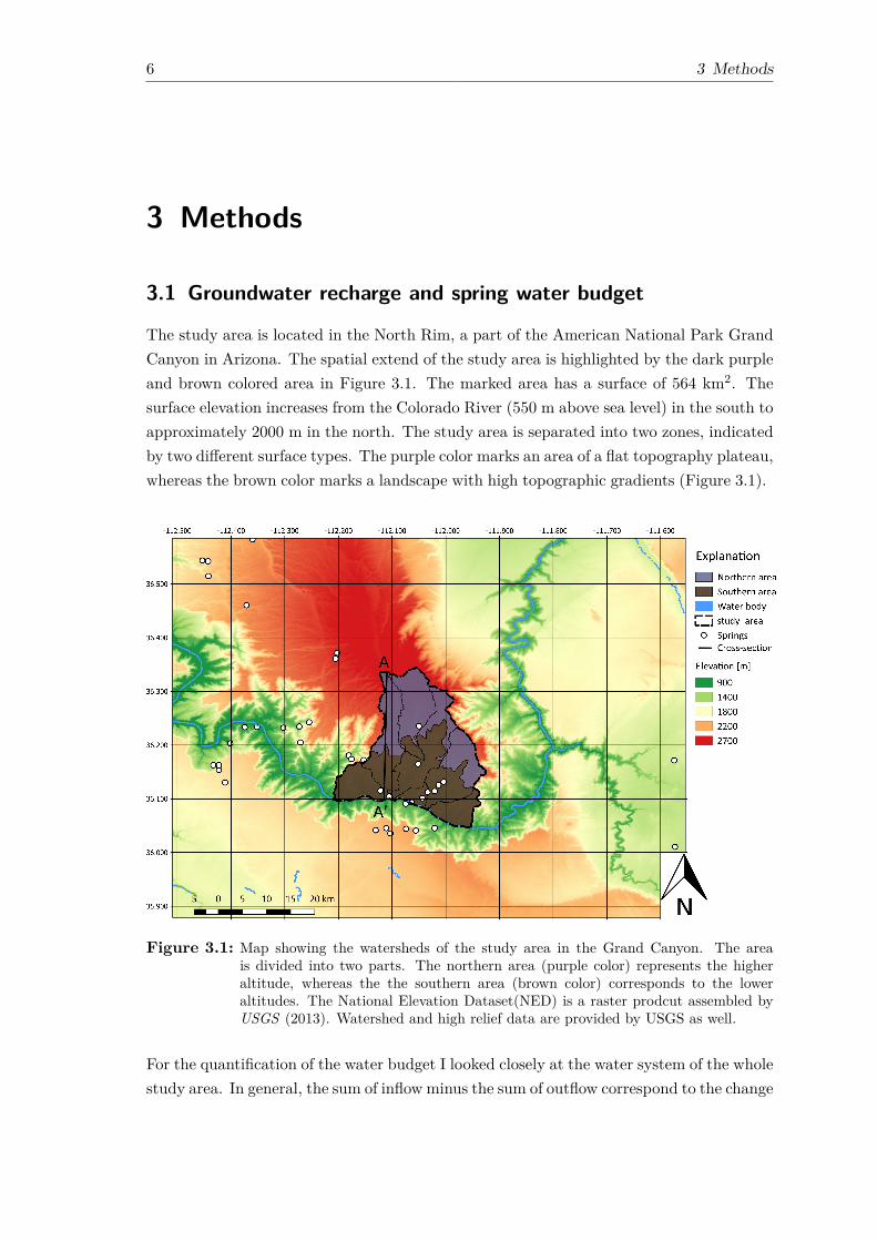
The study area is located in the North Rim, a part of the American National Park GrandCanyon in Arizona. The spatial extend of the study area is highlighted by the dark purpleand brown colored area in Figure 3.1. The marked area has a surface of 564 km2. Thesurface elevation increases from the Colorado River (550 m above sea level) in the south toapproximately 2000 m in the north. The study area is separated into two zones, indicatedby two different surface types. The purple color marks an area of a flat topography plateau,whereas the brown color marks a landscape with high topographic gradients (Figure 3.1).

Figure 3.1: Map showing the watersheds of the study area in the Grand Canyon. The areais divided into two parts. The northern area (purple color) represents the higheraltitude, whereas the the southern area (brown color) corresponds to the loweraltitudes. The National Elevation Dataset(NED) is a raster prodcut assembled byUSGS (2013). Watershed and high relief data are provided by USGS as well.

For the quantification of the water budget I looked closely at the water system of the wholestudy area. In general, the sum of inflow minus the sum of outflow correspond to the change

7 3 Methods

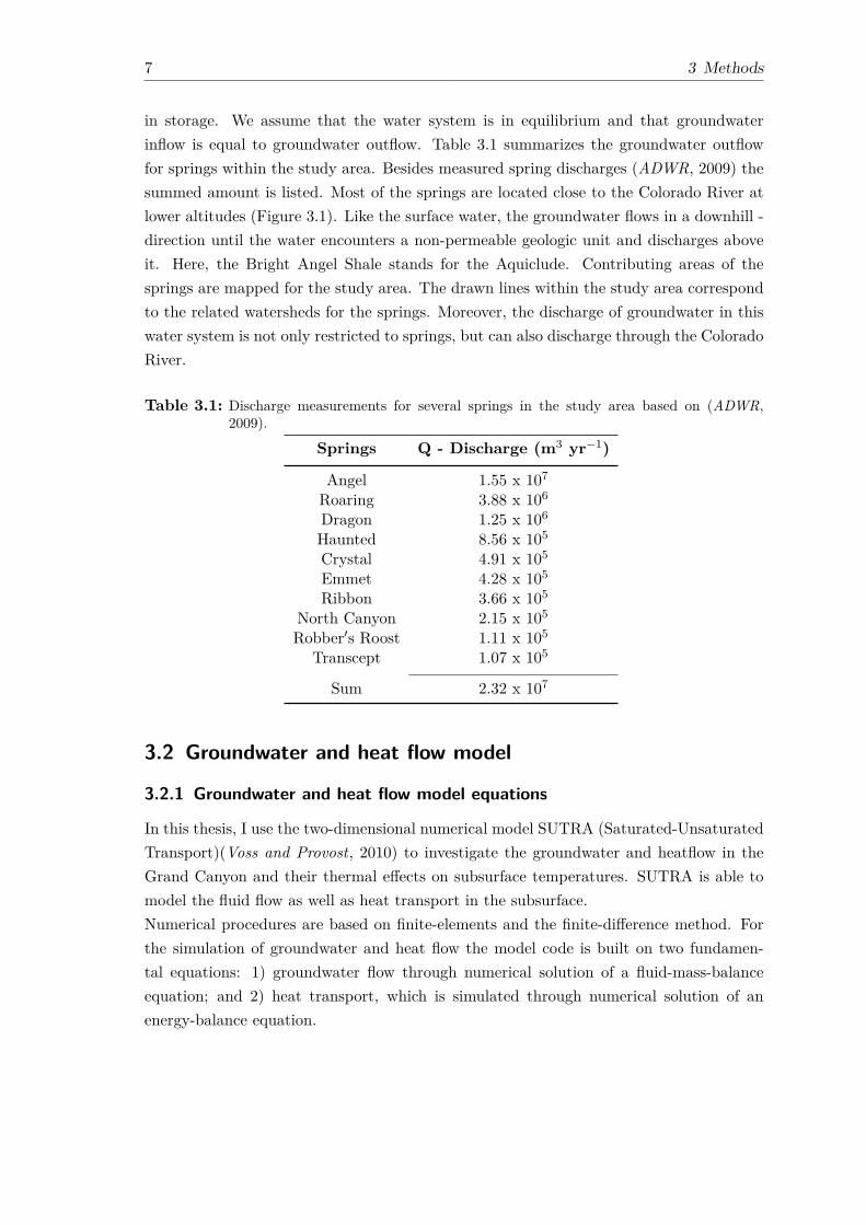
in storage. We assume that the water system is in equilibrium and that groundwaterinflow is equal to groundwater outflow. Table 3.1 summarizes the groundwater outflowfor springs within the study area. Besides measured spring discharges (ADWR, 2009) thesummed amount is listed. Most of the springs are located close to the Colorado River atlower altitudes (Figure 3.1). Like the surface water, the groundwater flows in a downhill -direction until the water encounters a non-permeable geologic unit and discharges aboveit. Here, the Bright Angel Shale stands for the Aquiclude. Contributing areas of thesprings are mapped for the study area. The drawn lines within the study area correspondto the related watersheds for the springs. Moreover, the discharge of groundwater in thiswater system is not only restricted to springs, but can also discharge through the ColoradoRiver.

Table 3.1: Discharge measurements for several springs in the study area based on (ADWR,2009).

Springs Q - Discharge (m3 yr−1)

Angel 1.55 x 107

Roaring 3.88 x 106

Dragon 1.25 x 106

Haunted 8.56 x 105

Crystal 4.91 x 105

Emmet 4.28 x 105

Ribbon 3.66 x 105

North Canyon 2.15 x 105

Robber′s Roost 1.11 x 105

Transcept 1.07 x 105

Sum 2.32 x 107

3.2 Groundwater and heat flow model

3.2.1 Groundwater and heat flow model equations

In this thesis, I use the two-dimensional numerical model SUTRA (Saturated-UnsaturatedTransport)(Voss and Provost, 2010) to investigate the groundwater and heatflow in theGrand Canyon and their thermal effects on subsurface temperatures. SUTRA is able tomodel the fluid flow as well as heat transport in the subsurface.Numerical procedures are based on finite-elements and the finite-difference method. Forthe simulation of groundwater and heat flow the model code is built on two fundamen-tal equations: 1) groundwater flow through numerical solution of a fluid-mass-balanceequation; and 2) heat transport, which is simulated through numerical solution of anenergy-balance equation.

8 3 Methods

A simplified form for the fluid mass balance can be written as:

So∂h

∂t−∇(K∇h) = Q∗ eq. 3.1

where Q∗ = (Qp

ρ )

and So(x,y)describes the specific storativity [m−1], h(x,y,t) is the hydraulic head as a sum ofpressure head and elevation head [m], t is the time [s], K(x,y) is the hydraulic conductivity[m s−1], Q∗(x,y) is the volumetric fluid source[s−1], Qρ(x,y) is the fluid mass source[kg/(m3

s)] with a more detailed description of the (mass fluid injected per time/volume aquifer)and ρ is the fluid density [kg/m3]. The equation is used under the assumption of sat-urated conditions. Further assumptions are the constant solute concentration and theconstant fluid density, and using the definition of hydraulic conductivity, K ≡ (kρg)/µ,where g represents the acceleration of gravity. The hydraulic head is defined as h ≡ hp

+ ELEVATION, where the pressure head, hp ≡ p/(ρg) (Voss and Provost, 2010). Theenergy-balance is expressed as:

∂[ρew + (1− ε)ρses]∂t

=−∇ (ρewv) +∇ · [µI · ∇T ] +∇ · [ρcwD · ∇T ] eq. 3.2

+QpcwT∗ + ργwo + (1− ε)ρsγso

where the first expression on left side of the equal-sign stands for the change of energy inthe solid matrix and the fluid over a period of time. The stored energy for a particularvolume are expressed by variables of eW is the energy per unit mass water [kg m2 s−2/kg],es is the energy per unit mass solid matrix [kg m2 s−2/kg] and ρes is the density of solidgrain in solid matrix [kg/m3].Following terms can influence the stored energy with time: λ(x, y[, z], t) is the bulk thermalconductivity of solid matrix plus fluid [kg m2 s−2/(s·m·◦C)], I is the dimensionless identytensor, cw is the specific heat of water [kg m2 s−2/kg·◦C], D is the dispersions tensor[m2/s], T ∗(x,y[,z],t) is the temperature of the source fluid [◦C],Yw 0(x,y[,z],t) is the energysource in the fluid [kg m2 s−2/(kg ·s)], Ys 0(x,y[,z],t) is the energy source in the solid grains[kg m2 s−2/(kg· s)]. The term of Qp expresses the energy production which are added dueto the fluid source with temperature Q∗.Figure 3.2 shows a simplified geometry of the model that is based on the defined cross-section. The required boundary conditions include that the cross-section is being perpen-dicular to the axis of the geologic units as well as the spatial proximity of springs. Theprofile has a length of 23700 m from south to north while the maximum height in the north-ern part of the cross-section is nearly 2800 m. As shown in Figure 2.1, the model domain isdetermined by different lithologic units and boundary conditions (see section 2.1). Figure

9 3 Methods

3.1 show several arrows which indicate the intended flow direction. To quantify this flowbehaviour I focus in particular on influecing factors of the permeability and the groundwa-ter recharge. The latter approach is favoured by the fact that the permeability representsa part of hydraulic conductivity (Freeze and Cherry, 1979) and therefore is linked to het-erogeneity of the porous material (Durner , 1994). The groundwater recharge, in turn,shows a large reliance on the climatological conditions over the related period of time.Furthermore, the topography effect of the study area is also relevant to the groundwaterrecharge, as groundwater can trickle away into the ground or a surface runoff takes place(see section 3.1 for further explanations). Likewise, the permeability of each lithologicalunit is also debated in section 3.2.2.

Figure 3.2: Sketch showing the model setup and the adjacent boundary conditions that arepresent along the identified cross-section.

3.2.2 Permeabilites of lithologic units

Considering the hydraulic characteristics of the lithostratigraphical units, the permeabilityof porous media is relevant to quantify the groundwater flow. Kozeny (1927) and Carman(1937) show that the expression of permeability is related to the porosity and the poresize. By setting the porosity to a fixed value of 10% for each cell simplifies the simulationand calibration of the permeability. Nevertheless, permeability is difficult to quantify,especially if one considers that the orders of magnitude ranges over more than 13 and thatflow direction depends on the heterogeneity (Gleeson et al., 2011; Freeze and Cherry, 1979).In this study, the permeabilities at regional scales are quantified by the numerical model.Gleeson et al. (2011) provide geometric mean of permeability values for hydrolithologiesand combined hydrolithologies in regional-scale. Based on their dataset, I was able toadjust the permeability for the lithologies in the numerical model. The datasets serve asinitial values for the permeabilities of our layers. With exception of the shale componentthe second column of Table 3.2 summarizes the geometric mean logarithmic permeabilityby Gleeson et al. (2011). The permeability value for the shale in this column is provided

10 3 Methods

by Neuzil (1994). The third column lists the standard deviations, which are related tovalues of Column 1. Additionally, the fault zone (see Figure 3.2 and 3.3) have to beconsidered. According to Bense et al. (2013), the permeability of a fault adjacent to theirrock can decrease by 2-3 orders of magnitude. This can lead to strong hydrogeologicalheterogeneities. The final adjustments of my best model fit are conducted by means ofnumerical modelling in Sutra and are shown in Table 4.2.

Table 3.2: Geometric mean logarithmic permeabilities for model adjustments and standard de-viations based on references of 1 = (Gleeson et al., 2011), 2 = (Neuzil, 1994).

Lithology logk (m2) σ References

Toroweap & Kaibab Formation -15.2 2.5 1Coconino & Tapeats Sandstone -12.9 0.9 1Supai Group & Hermit Formation -15.2 2.5 1Redwall-Muav Aquifer -11.8 1.5 1Bright Angle Shale -19 − 2Tapeats Sandstone -12.9 0.9 1Middle Proterozoic Sedimentary Rocks -15.2 2.5 1Early Proterozoic Crystalline Rocks -14.1 1.5 1

3.2.3 Model boundaries and initial conditions

In the calibrated numerical model the thermal boundary conditions are imposed at (1) thetop of the model, temperature (T) = 10◦C, which is derived as specified average annualsurface temperature for the entire upper model boundary; and (2) at the bottom of themodel a constant heat flow of 65 mW s−2 is assigned (Pollack et al., 1993). The left andthe right model sides do not exhibit boundary conditions. The boundary conditions for thegroundwater are applied along the flat plateau area of the model (further explanations arementioned in the subchapter below). For a better understanding Figure 3.2 demonstrates,among other things, the setup for the boundary conditions.

3.2.3.1 Groundwater recharge

The groundwater recharge is one of those input data that plays a decisive role for thequantification of groundwater and heat flow, but is strongly influenced by the local cli-mate conditions. As reported by Kumar (2012), the direct effect of climate change ongroundwater depends on changes in volume and the distribution of groundwater recharge.The volume income for groundwater recharge is related to precipitation amounts, intensityrates and timing which indirectly affects the flux in subsurface.With respect to the boundary condition, the groundwater recharge at the surface is dividedinto two zones (see Figure 3.1). From x = 9050 m to 23700 m of the model, I have assigned aconstant value for groundwater recharge. In contrast, no groundwater recharge is assignedfrom x = 0 m up to 9050 m, assuming that most of the precipitation in areas with a hightopographic gradient is converted to surface runoff.

11 3 Methods

The literature values from De Graaf et al. (2015) represent a steady-state recharge inputover the time period of 1957 – 2002. According to this simplified high-resolution global-scale groundwater model the average groundwater recharge for present-day is 5 mm y−1.The extremely low recharge rates are due the arid climate conditions.For applications in Sutra I used a groundwater recharge of 41.3 mm y−1, which are calcu-lated on the basis of measured spring discharges (also discussed in section 4.1). Addition-ally, other literature values of groundwater recharge used are shown in Table 4.1.

3.2.4 Model discretization

The model simulation is based on a simplified two-dimensional-geometry. The mentionedequations (3.1) & (3.2) for the groundwater and heat flow are solved along the 2D-model.The model length is set to 23700 m in x-direction, while the height of the model domainreaches 2760 m in z−direction. The topography of the cross-section which is describedby the upper boundary varies from 750 m on the model’s left side up to 2760 m at themodel’s right side as shown in Figure 3.3. To obtain a good fit for the topography givencross-section of QGIS (Figure 1.1) I use 20 rectangles consisting of grid cells. The 20rectangles were subdivided in rows and columns. The cell size in width ranges from aminimum of 20 m to a maximum of 42 m per cell (Figure 3.3). The height of each cellvaries from 7.5 m up to 27.5 m.

Figure 3.3: Model domain contains stratigraphic units in simplified vertical extent and men-tioned horizontal lines which divide the rectangles. Not included are the elementoutlines.

The lithostratigraphic units in the model are in sequence from bottom to top the EarlyProterozoic Sedimentary Rocks, Middle Proterozoic Sedimentary Rocks, the Bright AngleShale, the Mississipian Redwall Muav, the Supai Group & Hermit Formation, the Coconinosandstone and the Toroweap & Kaibab Formation (see Figure 2.1). In contrast to theyounger and horizontal layers, the older proterozoic layers are dipping down at an angleof ∼ 35◦. Besides this layout, the grey marked line in Figure 3.2 represents a fault zone.Regarding the time discretization, the modeled time steps for paleozoic and present-day areset to 1 year to compare simulation results of equal stratigraphic settings under differentrecharge conditions.

3.2.5 Model calibration

The model calibration serves to optimize the numerical simulation of the thermal effectsof the groundwater and heat flow and the possible implications on thermochronologicaldatasets. First model simulations are focused on setting up a scenario which corresponds

12 3 Methods

to the present-day conditions. To ensure that the enviromental conditions reflect the actualsituation, I imported the related discretization of the determined cross-section from thestudy area into Sutra. Subsequently, I added parameters such as groundwater recharge,heat flow, porosity and thermal conductivty values. For the model calibration, values ofgroundwater recharge, discharge and permeability are of vital importance. On the basisof measured spring discharge (ADWR, 2009) and modeled groundwater recharge values Icalibrated the permeability for each lithologic unit.First attempts are based on the initial permeabilites of lithologic units given by Gleesonet al. (2011); Neuzil (1994). Given the high uncertainty of permeability, the standarddeviations are also taken into account. Moreover, I conducted a parameter study for thepermeability to evaluate the impact of varying permeability rates.Further scenarios deal with the influencing factors such as the porosity and thermal con-ductivity. For the porosity I simulated scenarios with initial values of 5% and 30%, whereasthe thermal conductivity are examined for values of 1.5 and 4. The great range of valuesshould provide a preferably great impact on the thermal effects.

3.2.6 Groundwater flow in the Pleistocene

Initially, the first scenario measurements are related to the present-day values whereas thefollowing scenarios intend to examine prior data with past fluid flows from the Pleistocene.Additionally, the evolution of groundwater and heatflow over a period of time provideuseful insights regarding the thermal effects. On the basis of data from Zhu et al. (2003)the paleorecharge rates for the Pleistocene were 2 to 3 times higher than nowadays. Thestudies on early paleorecharges are based on chloride mass balance method and chlorine-36 data and are made for the area of the Yucca Mountain in Nevada. The knowledge ofthe paleoclimate changes underpin previous assumptions about the groundwater rechargerates (Zhu et al., 1998). Therefore, I set up model scenarios with 2 to 3 times higherrecharge values of present-day conditions. Scenarios with 4 to 5 times higher groundwaterrecharge values provide a further evolution of the thermal effects of groundwater and heatflow and possible implications for the time of formation of the Grand Canyon.

13 4 Results

4 Results

4.1 Spring water budget

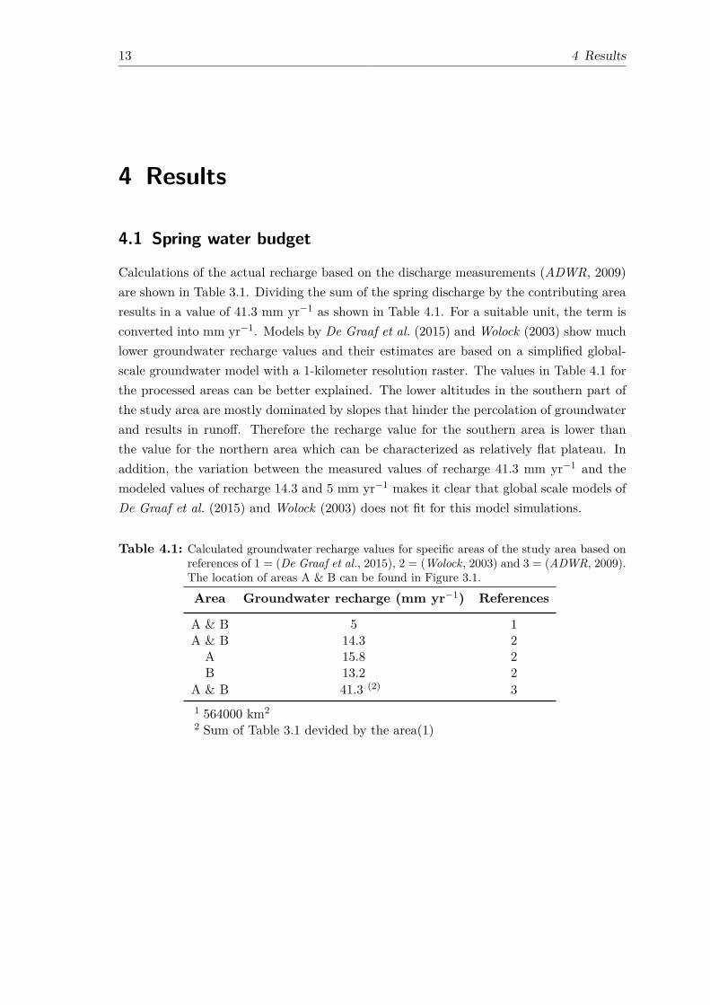
Calculations of the actual recharge based on the discharge measurements (ADWR, 2009)are shown in Table 3.1. Dividing the sum of the spring discharge by the contributing arearesults in a value of 41.3 mm yr−1 as shown in Table 4.1. For a suitable unit, the term isconverted into mm yr−1. Models by De Graaf et al. (2015) and Wolock (2003) show muchlower groundwater recharge values and their estimates are based on a simplified global-scale groundwater model with a 1-kilometer resolution raster. The values in Table 4.1 forthe processed areas can be better explained. The lower altitudes in the southern part ofthe study area are mostly dominated by slopes that hinder the percolation of groundwaterand results in runoff. Therefore the recharge value for the southern area is lower thanthe value for the northern area which can be characterized as relatively flat plateau. Inaddition, the variation between the measured values of recharge 41.3 mm yr−1 and themodeled values of recharge 14.3 and 5 mm yr−1 makes it clear that global scale models ofDe Graaf et al. (2015) and Wolock (2003) does not fit for this model simulations.

Table 4.1: Calculated groundwater recharge values for specific areas of the study area based onreferences of 1 = (De Graaf et al., 2015), 2 = (Wolock, 2003) and 3 = (ADWR, 2009).The location of areas A & B can be found in Figure 3.1.

Area Groundwater recharge (mm yr−1) References

A & B 5 1A & B 14.3 2

A 15.8 2B 13.2 2

A & B 41.3 (2) 31 564000 km22 Sum of Table 3.1 devided by the area(1)

14 4 Results

4.2 Simulations for the model calibration

The measured to calibrated spring discharge of the Dragon spring with values of 3.96x 10−5 m3 s−1 to 3.96 x 10−5 m3 s−1 agree well with each other. Best estimates ofpermeabilities for the calibration of discharge are listed in Table 4.2. In addition to thegeologic unis, the permeability value of -13.5 for the fault zone is also shown.

Table 4.2: Permeability values for lithologic units for the best model fit. Initial Geometric meanlogarithmic permeabilities and initial standard deviations and the Fault Zone basedon references of 1 = (Gleeson et al., 2011), 2 = (Neuzil, 1994), 3 = (Bense et al.,2013).

Lithology logk (m2) logk (m2) σ Referencescalibrated inital inital for initial k

Toroweap & Kaibab Formation -15.9 -15.2 2.5 1Coconino & Tapeats Sandstone -13.4 -12.9 0.9 1Supai Group & Hermit Formation -15.9 -15.2 2.5 1Redwall-Muav Aquifer -10.3 -11.8 1.5 1Bright Angle Shale -18.6 -19 − 2Tapeats Sandstone -13.4 -12.9 0.9 1Middle Proterozoic Sedimentary Rocks -15.34 -15.2 2.5 1Early Proterozoic Crystalline Rocks -14.3 -14.1 1.5 1Fault Zone -13.5 − − 3

The following results represent a quantification of the best model fit as well as the influenceof different parameters for the thermal effects of the entire model system. Figure 4.1and 4.3 show the output of model temperatures, permeabilities and flow vectors for thecalibrated 2D-cross-section model. The temperature field indicates a consistent horizontaltemperature gradation for almost the entire model length with exception of the area closeto the Colorado River, which describes an upwards trend towards the discharge sources.

Figure 4.1: Best-calibrated model simulation for the 2D-cross-section from the study area, show-ing the temperature profile with groundwater recharge conditions at present-day.The flow vectors indicate the groundwater flow directions.

The temperature increase with depth ranges from 10 ◦C to 36 ◦C on the right side to ∼25 ◦C to nearly 45 ◦C on the left side. However, it should be noted that the left side onlyhas an elevation of approximately 800 m, whereas the right side is more than 2700 m high.The observed temperature differences in Figure 4.1 lead to higher geothermal gradients inthe discharge area near to the Colorado River compared to the plateau area. Calculatedgeothermal gradients for locations of x = 0 m and x = 23490 m are ∼ 28 ◦C/km versus ∼

15 4 Results

10 ◦C/km verify these observations. Figure 4.2 validate the temperature evolution alongthe model domain. Graphs (a) and (b) show the subsurface temperature - depth relationfor the best model fit scenario at positions of x = 0 m and x = 23700 m. Both graphsshow lower temperatures at greater depth and increasing temperatures at lower depths.The temperature-depth curve in graph (a) is negative and reaches higher temperature atthe surface. In comparison, the curve in graph (b) is positive and reaches slightly lowertemperatures at the surface. This difference in fluid temperature over depth is due to thelimited groundwater recharge in the plateau area. As shown in Figure 4.1, groundwaterrecharge and the downwards directed groundwater flow is represented by the flow vectorswhich are restricted to the uppermost part of the model over the distance of x = 8000 m to23700 m. In the transition zone visualized by the color change from blue to turquoise theflow vectors change their flow direction towards the discharge area in the left. The reasonfor this change in orientation of the flow vectors is due the aquiclude (Bright Angel Shale),which is located above the turquoise layer. The lower amount of percolated groundwaterthrough the aquiclude flows in higher permeable units towards the area of the ColoradoRiver. The groundwater flow with an upwards trend in this area is highlighted in a largerscale in Figure 4.3. The observed temperature increase in this area is due to the upwardsflow of discharge areas like the Dragon spring (2) and the Colorado River (1) at the leftmargin.

Figure 4.2: Comparison of temperature-depth relations in the model at position (a) x = 0 mand (b) x = 23490 m.

Figure 4.4 illustrates the influence of different permeabilities for four specific geologicunits on discharge to the Colorado River and the Dragon spring. Changing the values ofpermeabilities of the geologic units of Redwall-Muav-Aquifer (a), Bright Angle Shale (b)and the Early Proterozoic Sedimentary Rocks (d) show no influence on the discharge ofthe Dragon-spring and the Colorado River. The Middle Proterozoic Sedimentary Rocksshow an exception with regard to interactions between permeability and discharge. Withincreasing permeability, logk values under -13.9 lead to a discharge of groundwater intothe Colorado River.Comparing the calibrated best model fit scenario with Figure 4.5 helps to understand theevolution of modeled temperature with and without groundwater recharge. In contrast

16 4 Results

Figure 4.3: Section of the discharge area with locations of the Colorado River (1) and the Dragonspring (2). Best-calibrated model simulation showing the temperature profile withgroundwater recharge conditions at present-day and flow vectors for the groundwaterflow direction.

Figure 4.4: The relation between discharge of the Dragon Spring (blue) and the Colorado River(red) to Permeability for specific lithologic units (a) Redwall-Muav-Aquifer, (b)Bright Angle Shale, (c) Early Proterozoic Sedimentary Rocks and (d) Middle Pro-terozoic Sedimentary Rocks. The Permeability is plotted on the x-axis and thedischarge is plotted on the y-axis. The blue dots, which are connected with lines,show calculated discharge values of several permeability settings for the Dragonspring, whereas the red dots represent the Colorado River.

17 4 Results

to the first mentioned scenario Figure 4.5, shows a linear temperature field, where thewhole system is only controlled by heat conduction. The comparison of both scenariosclearly illustrates cooling effects of groundwater flow on the Colorado Plateau and heatingof groundwater near the discharge zones.

Figure 4.5: Modeled temperature trend for groundwater recharge scenario = 0 mm yr−1.

The comparison of a groundwater recharge and a non-groundwater recharge scenario isshown in temperature difference over depth plots for the left (a) and right side (b) of themodel domain(see Figure 4.6). Graph (a) shows that the differences in temperature varybetween 10 to 14◦C over a depth of 800 m. Graph (b) depicts a difference of temperaturevalues of up to -32◦C over a depth of 2800 m. Therefore, the left-hand side of the modelis warmer in the groundwater flow scenario, whereas the right-hand side of the model iscooler.

Figure 4.6: Showing the temperature difference of a groundwater recharge scenario (41.3 mmyr−1) versus a non-groundwater recharge (0 mm yr−1) scenario in depth. Graph (a)represents a depth-profile for position x = 0 and (b) for position x = 23490 m.

Further parameters with a crucial meaning for the sensitive analysis of modeled temper-ature in the subsurface are the porosity, the thermal conductivity of the rock matrix andthe bulk thermal conductivity. Previous results were based on a constant porosity valueof 10% for the complete model area to keep the model as simple as possible and to focuson groundwater recharge, permeability and heat flow. To estimate the impact of varyingporosity values, Figure 4.7 shows scenarios with porosity values of 5% and 25%. This widerange serves to simulate the greatest possible and realistic impact of porosity on modeledtemperature. The model results of Figure 4.7 (a) and (b) show higher temperatures for aporosity value of 25%. In contrast to the 5% porosity model scenario the left corner of the

18 4 Results

25% porosity model shows a higher temperature gradient. Further, the horizontal coloredtemperature transition zones are slightly shifted upwards in the 25% model scenario.

Figure 4.7: Two different rock properties, which are applied in each scenario to every litholog-ical unit. The shown temperature profiles demonstrate the difference between rockproperties for the porosity of (a) = 5% and (b) = 25%. Flow vectors demonstratethe groundwater flow directions.

Figure 4.8 (a) and (b) examines the thermal conductivity of the rock matrix. In comparisonto snapshot (b) shows snapshot (a) a very pronounced development of temperature in theleft corner of the model along with the bottom domain of the model. Furthermore, thesnapshot (a) shows a larger cooling-off area which last to a depth of∼ 1200 m in comparisonto snapshot (b). With increasing temperatures starting at 10 ◦C, we can observe a stronglyrising geothermal gradient. In contrast, snapshot (b) increases early, but represents a lowergeothermal gradient and only reaches temperature values of approximately 35 ◦C at thebottom of the model.

Figure 4.8: Two different rock properties, which are applied in each scenario to every litholog-ical unit. The shown temperature profiles demonstrate the difference between rockproperties for the thermal conductivity of the rock matrix (a) = 1.5 and (b) = 4.Flow vectors demonstrate the groundwater flow directions.

Explanations for these temperature variations might be the interaction of the heat flowboundary condition at the bottom domain and the thermal conductivity values. Higherthermal conductivities result in a cooling effect, whereas lower thermal conductivitiesresult in an increase of temperature.

19 4 Results

Figure 4.9 demonstrates the relation of hydraulic head versus depth for positions (a)x = 0 m and (b) x = 23490 m. Graph (a) shows a groundwater flow upwards. Thegroundwater flow for graph (b) indicates a downward trend, which encounters an area offewer calculation points which is due to the less permeable zone of the Bright Angel Shale.The effect of the low permeability aquiclude (Bright Angel Shale) can be seen in Figure4.9 (b), as the the hydraulic head is decreasing from the top of the shale to the base ofthe shale from 3000 m to 1000 m respectively. The velocity vectors in Figure 4.1 clearlyshow that discharge of fluids is guided by the aquiclude towards the Canyon. Moreover,the aquiclude acts as a low permeability cap prohibiting high fluid flow across the BrightAngel Shale.

Figure 4.9: Two hydraulic head versus depth plots, showing the potential energy of the waterfor positions of (a) x = 0 m and (b) x = 23490 m in the model domain.

20 4 Results

In Figure 4.10, the Velocity of the groundwater is plotted against the depth at position (a)x = 0 m and (b) x = 23490. Here, positive values correspond to upward groundwater flowand negative values to downward groundwater flow. On the one hand, graph (a) describesincreasing velocities towards the upper model domain due to the discharge area. On theother hand, graph (b) slows down from top to bottom on the basis of groundwater rechargeat the surface. Smaller fluctuations in the course of the graph (b) can be explained bydeviation in permeability of the lithological units. Moreover, the outliners seen in graph(a) and (b) are caused by numerical instability of the model.

Figure 4.10: Velocity-Depth relationship for position (a) x = 0 m and (b) x = 23490 in themodel domain. Graph (a) shows increasing velocities towards the upper modeldomain, whereas the graph (b) slows down towards the bottom model domain.

21 4 Results

4.3 Groundwater flow in the Pleistocene

To quantify the impact on the temperature field, I examined the influence of groundwaterrecharge, as well as the amount of groundwater recharge which feeds the model. Figure4.11 and 4.12 represent six model scenarios with groundwater recharges of 20(a), 40(b),80(c), 120(d), 160(e) and 200(f) mm yr−1.Comparing these groundwater recharge scenarios, it is noticeable that temperature de-creases towards the bottom of the model. This cooling effect increases with groundwaterrecharge and appears along the entire model length. The discharge area close to the Col-orado River is also affected but not to such a great extent. Additionally, this evolutionof scenarios reflects a more and more groundwater dominated system. The Scenarios ofFigure 4.12 (e) and (f) should be highlighted, since these correspond to late Pleistocenegroundwater recharge conditions (Zhu et al., 2003). Moreover, the lower geothermal gra-dients with values of ∼ 23 ◦C/km and ∼ 6 ◦C/km at locations of x = 0 m and 23490m locations, in contrast to present-day geothermal gradients with values of ∼ 28 ◦C/kmand ∼ 10 ◦C/km confirm previous observed evolutions. It can be noted that the surfaceboundary condition of groundwater recharge for the plateau area is decisive for the changeof temperature from top to bottom of the model.Figure 4.13 which describes the relation between groundwater recharge and average tem-perature, confirms that we have a cooling effect of temperature with increasing ground-water recharge into the numerical model. The horizontal lines are representative for thepresent and past-day groundwater recharge conditions and clarify the difference in coolingbetween both scenarios.

Figure 4.11: Modeled groundwater recharge scenarios versus average temperature using temper-ature profile at position x = 23490 m. Horizontal lines are showing the estimatedvalues for present-day (1) and Pleistocene (2) groundwater recharge scenarios.

224

Results

Figure 4.12: Modeled groundwater flow and temperature trends for groundwater recharge scenarios of (a) 20 mm yr−1, (b) 40 mm yr−1 and (c) 80mm yr−1. Flow vectors demonstrate the groundwater flow directions.

234

Results

Figure 4.13: Modeled groundwater flow and temperature trends for groundwater recharge scenarios of (d) 120 mm yr−1, (e) 160 mm yr−1 and (f)200 mm yr−1. Scenario (d) and (e) represent the groundwater flow in the Pleistocene (Zhu et al., 2003). Flow vectors demonstrate thegroundwater flow directions.

24 5 Discussion

5 Discussion

The model approach (Table 4.2) shows a good fit for the calibration of permeabilitiesof present-day condition using modeled and measured discharge. Figure 6 indicates thedistribution of temperature for the whole model domain as well as the flow directionof the groundwater system is represented by the flow vectors. The conduction of heatis heterogeneous, since the model undergoes advective cooling almost exclusively whichis due to the topography-driven groundwater flow spreading consistently into the depthof the model. In contrast, the left margin of the model is heated which is due to theupwards flow caused by discharges into the Colorado River and the Dragon spring (Figure4.9). Although simulations of Figure 4.4 demonstrate that the permeability near to thedischarge sources is highly sensitive leading to different flow paths and other dischargelocations.The comparison of a none and existent groundwater recharge scenario shows that thegroundwater recharge significantly changes the temperature field of the model. First, thelinear temperature field (Figure 4.5) alters into a heterogeneous temperature field. Second,the best-model fit has an average cooling rate of up to 32 ◦C at the bottom of the modeland the heating in the discharge area suggest temperatures of approximately 14 ◦C. Bysimulations of increasing groundwater recharge (Figure 4.12 & 4.13) we ensure past-timegroundwater recharge scenarios. Shown results in previous mentioned figures in additionto figure 4.11 indicate a cooling effect that increases with higher groundwater rechargevalues. This evolution can be also described by decreasing geothermal gradients from ∼28 ◦C/km to ∼ 23 ◦C/km and from ∼ 10 ◦C/km to ∼ 6 ◦C/km for locations of x = 0 mand 23490 m. Further changes in temperature and their associated implications can beobtained, if the values of porosity and thermal conductivity are set differently (Figure 4.7& 4.8). In comparison to porosity value of 5%, a value of 25% result in higher temperatureincrease in the discharge area. Porosity values of 25% show in the discharge area a highertemperature increase in comparison to porosity value of 5%. The thermal conductivityshow with 1.5 higher temperature increases along the model domain, and especially in thedischarge area in comparison to the scenario with a thermal conductivity with a value of 4.Simulations for the thermal conductivity of the rock matrix result in higher temperatureincreases for a value of 1.5 compared to a value of 4. This temperature behaviour is due tothe greater interaction between the heat flow boundary condition at the bottom of domainand a lower bulk rock thermal conductivity.Furthermore, the groundwater recharge values for the best model fit vary a lot (see section4.1). The range between the measured (ADWR, 2009) 41.3 mm yr−1 and the calculated

25 5 Discussion

global scale models with 5 and 14.3 mm yr−1 from De Graaf et al. (2015) and Wolock(2003) differ a lot in this model which can be due to implications of arid climate conditions.Above all, the parameter of groundwater recharge implies a significant role in space andtime. The thermal system without groundwater mainly consist of an original presumedbasal heat flow as sole heat conductor that shifts towards a system that adds a groundwaterdominated cooling component by topography-driven groundwater flow. Nevertheless, weexperience heating due to upwards flow of groundwater in the discharge area. The impactof the strongly related groundwater recharge is higher for past – times (Pleistocene) incomparison to present-day, which should be considered for assumptions of exhumationsrates at the time of formation.

26 6 Conclusion

6 Conclusion

In this study a 2-D numerical model of groundwater and heat flow for a specific cross-section of the Grand Canyon is presented. To reproduce lithological characteristics forpresent-day conditions a relatively simple method is successfully used; available springdischarge data of the study area is adjusted to modeled spring discharge data by calibratingpermeability values for each geologic unit. The best-model fit shows a topography-drivengroundwater flow system that strongly affects the temperature field of the subsurface.The modeled temperature field shows a cooling effect up to 32 ◦C at the bottom of themodel which occurs for almost the entire model lenght with exception of the dischargearea close to the Colorado River. Besides this, the groundwater experiences a heating of∼ 14 ◦C at the left margin due to the upwards flow towards discharge sources. Here, thegeothermal gradient can also vary, if the highly sensitive permeability is slightly changedand the groundwater system discharges more through the Colorado River than throughthe spring.By choosing fixed values of 10% and 3.5 for parameters of the porosity and thermalconductivity, the model setup ensures a simplified calibration only by means of perme-ability which nonetheless remains realistic. The thermal effect of previously mentionedparameters are also simulated and should not be neglected but are not heterogeneouslyimplemented into the calibrated model. Furthermore, the comparison of a none and ex-istent groundwater recharge scenario highlights the thermal effects. A system withoutgroundwater recharge consists of a linear heat conductivity caused by a basal heat flow,whereas present groundwater recharge leads to advective cooling by topography-drivengroundwater flow and heating by upwards groundwater flow. The simulation results withhigher groundwater recharge scenarios demonstrate increasing topography-driven ground-water flow that leads to a greater cooling effect and therefore to a greater thermal effectin times of the Pleistocene. Geothermal gradients in space and time confirm the observedtemperature evolutions. The geothermal gradient of the discharge area close to the Col-orado River decreases from ∼ 28 ◦C/km to ∼ 23 ◦C/km and the geothermal gradient forthe plaetau area decreases from ∼ 10 ◦C/km to ∼ 6 ◦C/km for the present to past-daygroundwater recharge conditions.In conclusion, the results points strong thermal effects that are related to topography-driven groundwater flow. Special attention should be given to the heterogonous temper-ature field which implies a cooling for almost the entire model with exception for thedischarge area around the Colorado River which undergoes heating. Additionally, greatergroundwater recharge scenarios suggest that the thermal effects were even more signifi-

27 6 Conclusion

cant in the past. Thus, the results show that groundwater and heat flow with alteringtemperatures in time and space plays an important role in the thermal history and shouldbe included in studies regarding the time of formation for the Grand Canyon that relyalmost exclusively on low-temperature thermochronology.The model simulations can be seen as a first-order attempt towards groundwater andheat flow modeling with regards to the influence of thermal effects. However, they havetheir limitations that hamper a completely trustworthy simulation. Further investigationsshould aim to improve the parametrizations of the model to capture the full structuralcomplexity. Terms which should be considered are: heterogeneities of layers, faults andtheir location, spreading of sinkholes and joints, specified porosities for each layer insteadof a simplified model-wide value as well as the chemical composition of aqueous fluids.

28 Bibliography

Bibliography

ADWR, A. D. o. W. R. (2009), Arizona Water Atlas Volume 6 Western Plateau PlanningArea, 297 pp., available at http://www.azwater.gov/AzDWR/StatewidePlanning/

WaterAtlas/WesternPlateau/default.htm, last accessed on 08.09.2017.

Anderson, M. P. (2005), Heat as a Ground Water Tracer, Ground Water, 43 (6), 951–968,doi:10.1111/j.1745-6584.2005.00052.x.

Bense, V. F., T. Gleeson, S. E. Loveless, O. Bour, and J. Scibek (2013), Fault zonehydrogeology, doi:10.1016/j.earscirev.2013.09.008.

Beus, S. S., and M. Morales (2003), Grand Canyon Geology, 432 pp., Oxford UniversityPress.

Carman, P. C. (1937), Fluid flow through granular beds, Institution of Chemical Engi-neeres.

De Graaf, I. E. M., E. H. Sutanudjaja, L. P. H. Van Beek, and M. F. P. Bierkens (2015), Ahigh-resolution global-scale groundwater model, Hydrology and Earth System Sciences,19 (2), 823–837, doi:10.5194/hess-19-823-2015.

Durner, W. (1994), Hydraulic conductivity estimation for soils with heterogeneous porestructure, Water Resources Research, 30 (2), 211–223, doi:10.1029/93WR02676.

Farley, K. A. (2000), Helium diffusion from apatite: General behavior as illustrated byDurango fluorapatite, Journal of Geophysical Research: Solid Earth, 105 (B2), 2903–2914, doi:10.1029/1999JB900348.

Foos, A. (1999), Geology of Grand Canyon National Park , North Rim.

Freeze, R. A., and J. A. Cherry (1979), Groundwater, 1–624 pp.

Gleeson, T., L. Smith, N. Moosdorf, J. Hartmann, H. H. Durr, A. H. Manning, L. P. H.Van Beek, and A. M. Jellinek (2011), Mapping permeability over the surface of theEarth, Geophysical Research Letters, 38 (2), 1–6, doi:10.1029/2010GL045565.

Hill, C. A., and V. J. Polyak (2010), Karst hydrology of Grand Canyon, Arizona, USA,Journal of Hydrology, doi:10.1016/j.jhydrol.2010.06.040.

Hill, C. A., et al. (2016), The Grand Canyon : monument to an ancient Earth : canNoah’s flood explain the Grand Canyon?

29 Bibliography

Huntoon, P. W. (1974), The karstic groundwater basins of the Kaibab Plateau, Arizona,Water Resources Research, 10 (3), 579–590, doi:10.1029/WR010i003p00579.

Huntoon, P. W. (2000a), Karstification associated with groundwater circulation throughthe Redwall Artesian Aquifer, Grand Canyon, Arizona.

Huntoon, P. W. (2000b), Variability of karstic permeability between unconfined andconfined aquifers, Grand Canyon region, Arizona, Environmental & Engineering Geo-science, 6 (2), 155–170, doi:10.2113/gseegeosci.6.2.155.

Ingraham, N. L., K. Zukosky, and D. K. Kreamer (2001), Application of Stable IsotopesTo Identify Problems in Large-Scale Water Transfer in Grand Canyon National Park,doi:10.1021/ES0015186.

Irvine, D. J., R. H. Cranswick, C. T. Simmons, M. A. Shanafield, and L. K. Lautz (2015),The effect of streambed heterogeneity on groundwater-surface water exchange fluxesinferred from temperature time series, Water Resources Research, 51 (1), 198–212, doi:10.1002/2014WR015769.

Karlstrom, K. E., R. Crow, L. J. Crossey, D. Coblentz, and J. W. Van Wijk (2008), Modelfor tectonically driven incision of the younger than 6 Ma Grand Canyon, Geology, 36 (11),835, doi:10.1130/G25032A.1.

Karlstrom, K. E., et al. (2014), Formation of the Grand Canyon 5 to 6 million years agothrough integration of older palaeocanyons, doi:10.1038/NGEO2065.

Keshari, A. K., and M. Koo (2007), A numerical model for estimating groundwater fluxfrom subsurface temperature profiles, Hydrological Processes, 21 (25), 3440–3448, doi:10.1002/hyp.6577.

Ketcham, R. A., A. Carter, R. A. Donelick, J. Barbarand, and A. J. Hurford (2007),Improved modeling of fission-track annealing in apatite, American Mineralogist, 92 (5-6), 799–810, doi:10.2138/am.2007.2281.

Kozeny, J. (1927), Uber Kapillare Leitung der Wasser in Boden, Royal Academy of Science,Vienna, Proc. Class I, 136, 271–306.

Kumar, C. P. (2012), Climate Change and Its Impact on Groundwater Resources, 1 (5),43–60.

Metzger, D. G. (1961), Geology in Relation to Availability of Water Along the South RimGrand Canyon National Park Arizona, US Government Printing Office.

Neuzil, C. E. (1994), by Bethke permeability , measurements in Figure, Water Resources,30 (2), 145–150.

30 Bibliography

Pollack, H. N., S. J. Hurter, and J. R. Johnson (1993), Heat flow from the Earth’sinterior: Analysis of the global data set, Reviews of Geophysics, 31 (3), 267, doi:10.1029/93RG01249.

Price, L. G. (1999), An introduction to Grand Canyon geology, 63 pp., Grand CanyonAssociation.

Shuster, D. L., and K. A. Farley (2004), 4He/3He thermochronometry, Earth and Plane-tary Science Letters, 217 (1-2), 1–17, doi:10.1016/S0012-821X(03)00595-8.

USGS, U. S. G. S. (2013), National Elevation Dataset, available at https://lta.cr.

usgs.gov/NED, last accessed on 07.07.2017.

Voss, . I., and A. M. Provost (2010), SUTRA: a model for saturated-unsaturated, variable-density ground-water flow with solute or energy transport, Water-Resources Investiga-tions Report 02-4231, 2010, 300 p.

Wernicke, B. (2011), The California River and its role in carving Grand Canyon, GeologicalSociety of America Bulletin, 123 (7-8), 1288–1316, doi:10.1130/B30274.1.

Wolock, D. M. (2003), Estimated mean annual natural ground-water recharge in theconterminous United States, U.S. Geological Survey, (Open-File Rep 03–311, digitaldataset), available at https://pubs.er.usgs.gov/publication/ofr03311, last ac-cessed on 07.07.2017.

Zhu, C., R. K. Waddell, I. Star, and M. Ostrander (1998), Responses of ground water inthe Black Mesa basin, northeastern Arizona, to paleoclimatic changes during the latePleistocene and Holocene, Geology, 26 (2), 127, doi:10.1130/0091-7613(1998)026〈0127:ROGWIT〉2.3.CO;2.

Zhu, C., J. R. Winterle, and E. I. Love (2003), Late Pleistocene and Holocene groundwaterrecharge from the chloride mass balance method and chlorine-36 data, Water ResourcesResearch, 39 (7), doi:10.1029/2003WR001987.

I 7 Appendix

7 Appendix

Appendix Table .1: Modeled discharge values of the Colorado River and the Dragon springfor the Redwall-Muav-Aquifer at specific logk values.

Redwall-Muav-AquiferDragon Spring Colorado River logk (m2)

-3.956E-02 -4.173E-01 -10.3-3.956E-02 -4.173E-01 -10.6-3.957E-02 -4.173E-01 -10.9-3.957E-02 -4.173E-01 -11.2-3.957E-02 -4.174E-01 -11.5-3.957E-02 -4.174E-01 -11.8-3.957E-02 -4.174E-01 -12.1-3.957E-02 -4.174E-01 -12.4-3.957E-02 -4.174E-01 -12.7-3.957E-02 -4.174E-01 -13-3.957E-02 -4.174E-01 -13.3

Appendix Table .2: Modeled discharge values of the Colorado River and the Dragon springfor the Bright Angel Shale at specific logk values.

Bright Angel ShaleDragon Spring Colorado River logk (m2)

-3.958E-02 -4.173E-01 -17.9-3.958E-02 -4.174E-01 -18.1-3.957E-02 -4.174E-01 -18.3-3.957E-02 -4.174E-01 -18.5-3.957E-02 -4.174E-01 -18.7-3.957E-02 -4.174E-01 -18.9-3.957E-02 -4.174E-01 -19.1-3.957E-02 -4.174E-01 -19.3-3.957E-02 -4.174E-01 -19.5-3.957E-02 -4.174E-01 -19.7-3.957E-02 -4.174E-01 -19.9-3.957E-02 -4.174E-01 -20.1

II 7 Appendix

Appendix Table .3: Modeled discharge values of the Colorado River and the Dragon springfor the Middle Proterozoic Sedimentary Rocks at specific logk values.

Middle Proterozoic Sedimentary RocksDragon Spring Colorado River logk (m2)

-4.130E-01 -4.389E-02 -12.7-4.028E-01 -5.417E-02 -12.9-3.879E-01 -6.905E-02 -13.1-3.671E-01 -8.979E-02 -13.3-3.396E-01 -1.173E-01 -13.5-3.052E-01 -1.517E-01 -13.7-2.653E-01 -1.916E-01 -13.9-2.224E-01 -2.345E-01 -14.1-1.800E-01 -2.770E-01 -14.3-1.411E-01 -3.159E-01 -14.5-1.077E-01 -3.493E-01 -14.7-8.041E-02 -3.765E-01 -14.9-5.891E-02 -3.980E-01 -15.1-4.236E-02 -4.146E-01 -15.3-2.986E-02 -4.271E-01 -15.5-2.060E-02 -4.363E-01 -15.7-1.392E-02 -4.430E-01 -15.9-9.235E-03 -4.477E-01 -16.1-6.034E-03 -4.509E-01 -16.3-3.897E-03 -4.530E-01 -16.5-2.497E-03 -4.544E-01 -16.7-1.591E-03 -4.553E-01 -16.9-1.010E-03 -4.559E-01 -17.1-6.394E-04 -4.563E-01 -17.3-4.041E-04 -4.565E-01 -17.5-2.551E-04 -4.567E-01 -17.7

III 7 Appendix

Appendix Table .4: Modeled discharge values of the Colorado River and the Dragon springfor the Early Proterozoic Crystalline Rocks at specific logk values.

Early Proterozoic Crystalline RocksDragon Spring Colorado River logk (m2)

6.227E-07 -4.569E-01 -12.6-2.562E-06 -4.569E-01 -12.8-7.588E-06 -4.569E-01 -13-1.551E-05 -4.569E-01 -13.2-2.798E-05 -4.569E-01 -13.4-4.756E-05 -4.569E-01 -13.6-7.829E-05 -4.568E-01 -13.8-1.265E-04 -4.568E-01 -14-2.022E-04 -4.567E-01 -14.2-3.214E-04 -4.566E-01 -14.4-5.089E-04 -4.564E-01 -14.6-8.041E-04 -4.561E-01 -14.8-1.268E-03 -4.557E-01 -15-1.993E-03 -4.549E-01 -15.2-3.121E-03 -4.538E-01 -15.4-4.858E-03 -4.521E-01 -15.6

Appendix Table .5: Calculation of each heat flow rectangle for the bottom model boundarycondition.

Segment length Quantity Length (m) Cell length (m) Heat flow per rectangle

400 20 400 20 1.3600 8 200 25 1.6252100 60 1500 25 1.6252700 24 600 25 1.6254100 54 1400 25.92592593 1.6851851854500 16 400 25 1.6255000 18 500 27.77777778 1.8055555565400 14 400 28.57142857 1.8571428575800 14 400 28.57142857 1.8571428576200 12 400 33.33333333 2.1666666677100 26 900 34.61538462 2.257800 24 700 29.16666667 1.8958333338200 13 400 30.76923077 28400 7 200 28.57142857 1.8571428579050 20 650 32.5 2.112510050 25 1000 40 2.613500 86 3450 40.11627907 2.6075581415500 50 2000 40 2.619500 100 4000 40 2.623700 100 4200 42 2.73

IV 7 Appendix

Appendix Table .6: Calculation of the 5 groundwater recharge rectangles for the top modelboundary condition.

Rectangle Quantity Segment length Cell length

1 25 1000 402 86 3450 40.116279073 50 2000 404 100 4000 405 100 4200 42

V 7 Appendix

App

endi

xT

able

.7:

Gro

undw

ater

rech

arge

scen

ario

sw

ithth

eir

mm

yr−

1va

lues

,the

conv

ersio

nof

thes

ean

dca

lcul

ated

valu

esof

each

grou

ndw

ater

rech

arge

rect

angl

eat

the

top

mod

elbo

unda

ryfo

rsim

ulat

ions

inSu

tra.

Gro

undw

ater

rech

arge

Ref

eren

ces

De

Gra

afet

al.

2015

Wol

ock

2003

AD

WR

2009

Zhu

etal

.20

03m

myr−

15

14.3

41.3

2080

123.

916

020

0m

s−1

1.59

E-10

4.53

E-10

1.31

E-09

6.34

E-10

2.54

E-09

3.93

E-09

5.07

E-09

6.34

E-09

Rec

tang

le

16.

34E-

061.

81E-

055.

23E-

052.

54E-

051.

01E-

041.

57E-

042.

03E-

042.

54E-

042

6.36

E-06

1.82

E-05

5.25

E-05

2.54

E-05

1.02

E-04

1.57

E-04

2.04

E-04

2.54

E-04

36.

34E-

061.

81E-

055.

23E-

052.

54E-

051.

01E-

041.

57E-

042.

03E-

042.

54E-

044

6.34

E-06

1.81

E-05

5.23

E-05

2.54

E-05

1.01

E-04

1.57

E-04

2.03

E-04

2.54

E-04

56.

66E-

061.

90E-

055.

49E-

052.

66E-

051.

07E-

041.

65E-

042.

13E-

042.

66E-

04