Thermal Analysis of Composites Using DSC · Thermal Analysis of Composites Using DSC by Suchitra...

11

��

Thermal Analysis of Composites Using DSC by Suchitra Mutlur

Differential scanning calorimetry (DSC) is a technique that measures the difference in the heat flow to a sample and to a reference sample as a direct function of time or temperature under heating, cooling or isothermal conditions [1]. DSC is one of the most versatile thermal analysis techniques available. It can be used with composites and composite precursors to study thermodynamic processes (glass transition, specific heat capacity) and kinetic events such as cure and enthalpic relaxation associated with physical aging or stress [2]. The application of DSC to evaluate these material properties will be discussed in the following sections.

2.1 Background Thermal analysis is a family of techniques used for studying the thermophysical and kinetic properties of materials. The techniques include DSC; its advanced analog, modulated DSC (MDSC) (TA Instruments, New Castle, DE); thermomechanical analysis (TMA); dynamic mechanical analysis (DMA); and dielectric analysis (DEA). Thermal analysis can be used with composite materials to determine properties of the matrix material that are important for the analysis of the composite as a whole (especially where matrix dominated failures are likely to occur) [3].

The technique of DSC was introduced in the form of commercial instruments during the early 1960s, and it has been found to provide a convenient and useful method to measure the glass transition, melting, and crystallization temperatures of uncured prepregs and cured laminates, and also the degree of cure of the final product, the heat of reaction during prepreg processing, and relative resin reactivity. Its main advantages are the modest requirements in terms of sample size (~20 mg) and its ability to provide quantitative data on overall reaction kinetics, with relative speed and ease [2].

Advanced Topics in Characterization of Composites 12

2.2 Types of DSC There are two basic types of DSC systems: heat flux DSC and power compensation DSC [4]. Although fundamentally different in operation, they produce comparable data.

2.2.1 Heat Flux DSC The heat flux DSC belongs to the class of heat-exchanging calorimeters [5]. In the heat flux DSC, the sample and the reference are heated from the same source and the temperature difference is measured. This signal is converted to a power difference using the calibration sensitivity [4].

The characteristic feature of this measuring system is that the main heat flow from the furnace to the sample and reference containers passes symmetrically through a thermally conductive disk. The sample containers are positioned on this disk symmetrical to the center, and the temperature sensors are integrated. Each temperature sensor covers more or less the area of support of the respective container (crucible, pan) so that calibration can be carried out independent of the sample position inside the container. To minimize measurement uncertainties, the arrangement of the containers and the temperature sensors must always be the same [6,7]. Sometimes a center pin is used for the alignment of the sample and reference pan.

Metals, quartz glass, or ceramics are used as disk materials. Type (and number) of the temperature sensors (e.g., thermocouples, resistance thermometers) differ. The use of modern sensors on the basis of semi-conducting material leads to a significant increase in the sensitivity. Figure 2.1 shows the typical heat-flux DSC. The components are the (1) disk, (2) furnace, (3) lid, (4) differential thermocouple(s), (5) programmer and controller, (S) crucible with sample substance, and (R) crucible with reference sample substance. The heat flow rate from the furnace to the sample crucible is �FS; �FR is the heat flow rate from the furnace to the reference sample crucible; �m is the measured heat flow rate; and K is the temperature dependent calibration factor.

Thermal Analysis of Composites Using DSC 13

FIGURE 2.1

Heat flux DSC [3]

When the furnace is heated (typically a constant heating rate), heat flows through the disk to the samples. When the arrangement is ideally symmetrical (with samples of the same kind), the same heat flows into the sample and reference pans. The differential temperature signal �T (normally in the form of an electrical potential difference) is then zero. If this steady-state equilibrium is disturbed by a sample transition, a differential signal is generated that is proportional to the difference between the heat flow rates to the sample and to the reference sample [5]:

�T = TS - TR (2.1) where TS is the temperature of the sample and TR is the temperature of the reference sample.

As neither ideal thermal symmetry of the measuring system at all operating temperatures nor thermal identity of the samples can be attained in practical application, there will always be a signal �T that depends on the temperature and the sample properties. The heat flow rate �m (m: measured) is obtained by multiplying the differential temperature signal by factory-installed provisional calibration k' given as [5]:

�m = -k'· �T (2.2)

The measurement signal output by the DSC and accessible to the user is

�m (in µW or mW). Heat Flux DSC is available for temperatures between -190 oC and 1600 oC. The maximum heating rates are about 100 k/min.

T(t)

Computer K(T)

Recorder �m(T)

�T �m

4

2

1

S R

3

5

�FS �FR


2.2.2 Power compensated DSC The power compensation DSC belongs to the class of heat-compensating calorimeters. The heat to be measured is almost totally compensated with electric energy. The measuring system consists of two identical micro furnaces that are mounted inside a metal block. The furnaces (often made of a platinum-iridium alloy) each contain a temperature sensor and a heating resistor. The maximum heating power of a micro furnace is about 15W, and the maximum heating rate is 500 k/min. Cooling rate can reach up to 200 k/min, depending on the temperature difference between the block and sample. Figure 2.2 shows the block diagram indicating the basic operating principle. Here, Ts is the temperature of the sample furnace, TR is the temperature of the reference sample furnace, and PAV is the average heating power.

FIGURE 2.2

Power compensation DSC (Perkin-Elmer Instruments). During heating-up, the same heating power is supplied to both

microfurnaces via a control circuit in order to change their mean temperature in accordance with the preset heating rate. If there is ideal thermal symmetry, the temperature of both micro furnaces is always the same. When an asymmetry occurs, for example, as a result of a sample reaction, a temperature difference results between the microfurnace accommodating the sample and the microfurnace containing the reference sample. The temperature difference is both the measurement signal and the

Reference-furnace

PAV

�P

TS

TS

TR

�P

TR

T(t)

PAV

Calibration

(TS+TR)/2 control

(TS-TR) control

Recorder �m (t)

Sample- Furnace

Programmer

�T �m


input signal of a second control circuit. This second circuit compensates most of the reaction heat flow rate by proportional control by increasing or decreasing an additional heating power of the sample furnace. The compensating heating power, �P, is proportional to the remaining temperature difference, �T, because of the proportional controller. The time integral over the compensating heating power is proportional to the heat that was consumed or released in the sample.

Again, a heat flow rate �m is assigned to the real measurement signal �T as a result of a factory-installed calibration. The relations between �T, �m , and the compensating heating power �P are as follows [5]:

�P = -k1· �T (2.3)

�m = -k2· �T (2.4)

The factor k1 is a factory-set fixed quantity of the proportional controller, and k2 can be adjusted by software calibration. The factor k2 is almost independent of measurement parameters (e.g., temperature). Therefore, k2

can, in principle, be determined by one calibration measurement at only one temperature.

The relation between the measured heat flow rate, �m, and the true heat flow rate exchanged with the sample is

�true=K�·�m, (2.5)

and must also be determined by caloric calibration.

2.3 Applications of DSC Differential scanning calorimetry is the most popular thermal technique for polymer characterization. Uses for polymers include monitoring of cure of thermosetting resins, measuring the degree of cure of the final product, studying the crystallinity in thermoplastics, studying the compatibility of multiphase systems, and identifying transitions imposed upon the polymer by faulty processing or aging [3].

As the temperature of the sample is increased, the temperature is plotted on the x-axis and the difference in the heat flow between the sample and the reference on the y-axis [8].


2.3.1 Measurement of Heat Capacity of Composites (Cp) Heat capacity is an important material property for composites. Other than DSC, there is no other method which supplies the temperature dependent heat capacity as quickly and over such a large temperature range with sufficient accuracy. In a DSC, when the two pans are heated, the computer plots the difference in heat flow against temperature. So the heat absorbed by the polymer matrix is plotted against temperature, as given below [8]:

FIGURE 2.3

Heat flow rate measured by DSC*

The heat flow rate is shown in units of heat, q supplied per unit time, t

==dtdqϕ heat flow rate (2.6).

The heating rate, �, is the time rate of change of temperature, T [8]:

==dtdTβ heating rate (2.7).

The heat flow rate, �, divided by the heating rate, �, gives the heat capacity Cp:

==== pCdTdqdtdTdtdq

βϕ

heat capacity (2.8).

Therefore, the DSC plot gives the heat capacity of the sample. This plot of heat capacity is also required for the characterization of the glass transition process for polymer composites.

* Note: In some systems exothermic heat flow is shown up on the y-axis, while in other systems the exothermic direction is down on the y-axis.

exo

dq/dt

Temperature, T

Hea

t flo

w ra

te, �


2.3.2 Determination of Glass Transition temperature (Tg) Below a certain temperature, known as the glass transition temperature Tg, the polymer matrix segments do not have enough energy to rearrange or to rotate themselves. Such a material is brittle and a glass. As the sample is heated, there is a small increase in volume and energy, until at Tg the chains become more mobile and the polymer more plastic or rubbery. Also, the heat capacity of the sample increases, since the chains acquire further freedom of movement. Therefore, we observe a step and an increase �Cp, and also a change in the expansion [4]. The glass transition process does not involve a latent heat, and hence this transition is called a second order transition [7].

The physical properties such as hardness, volume, Young’s modulus, and percent elongation-to-break undergo a drastic change at the glass transition temperature of any amorphous polymer [9]. Figures 2.4 and 2.5 show the changes in the volume and modulus at the glass transition.

FIGURE 2.4 FIGURE 2.5 Typical volume change vs Typical modulus change vs temperature Ref [9] temperature Ref [9]

The glass transition region occurs over a temperature range. So, Tg is

typically defined as the point of inflection of the DSC curve, as illustrated in Figure 2.6. ASTM Standard Test Method E1356-03 gives further guidelines for assigning the glass transition temperature using DSC [10].

Mod

ulus

Temperature

Glassy Tg

Glassy

Rubbery

Vol

ume

Temperature Tg


FIGURE 2.6

Heat flow rate measured by DSC showing practical determination of Tg

Tg is a time-dependant phenomenon. A polymer may slowly distort at a low temperature, but may behave in a brittle fashion when bent rapidly. While the Tg bears a marked resemblance to true second-order thermodynamic transitions, which always occur over a fixed, equilibrium temperature range, the value obtained for Tg depends greatly on the heating and cooling rates used in the DSC run, molecular weight, plasticizer content, sample size, cross-linking, crystallinity, and degree of cure.

If the heating rate is very low, say 0.1 K/min, the Tg may be low, say 80 �C, and this value is obtained again if the sample is cooled at the same rate. However, if the sample is heated and cooled at 20 K/min, the Tg may increase to 85 �C or higher. If the heating and cooling rates are not the same, the sample that has been cooled slowly (say 0.1 K/min) goes through its Tg at 80 �C. If it is then heated at 20 K/min, it does not transform until 85 �C. This means that the sample must absorb more energy to reach the enthalpy of the rubbery state. This results in an endotherm, superimposed on the glass transition step, as shown in Figure 2.7. The heating and the cooling rates must therefore be stated [4].

FIGURE 2.7

DSC curve for polymer heated at a much lower rate than is was cooled Experimentally, Tg is a function of molecular weight. Enhanced

molecular weights increase Tg up to a plateau level. The rubbery nature of

Tg

Temperature

Hea

t flo

w ra

te, �

exo

exo

Hea

t flo

w ra

te, �

Temperature

Endothermic Peak


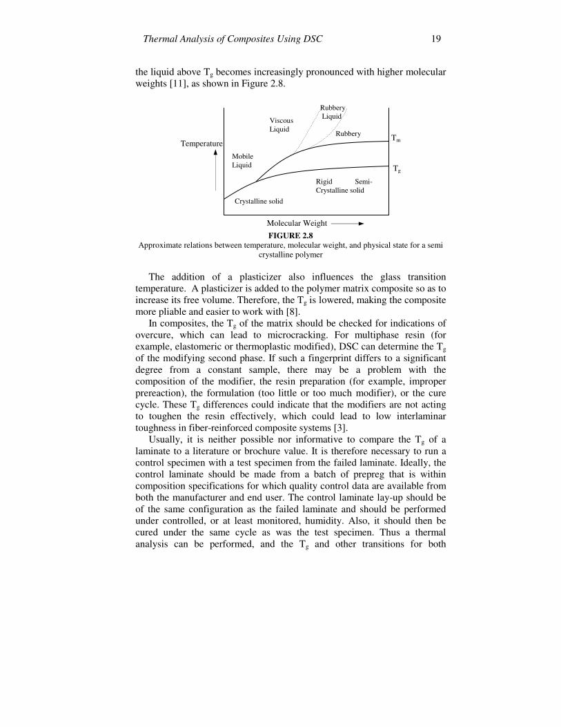
the liquid above Tg becomes increasingly pronounced with higher molecular weights [11], as shown in Figure 2.8.

FIGURE 2.8

Approximate relations between temperature, molecular weight, and physical state for a semi crystalline polymer

The addition of a plasticizer also influences the glass transition

temperature. A plasticizer is added to the polymer matrix composite so as to increase its free volume. Therefore, the Tg is lowered, making the composite more pliable and easier to work with [8].

In composites, the Tg of the matrix should be checked for indications of overcure, which can lead to microcracking. For multiphase resin (for example, elastomeric or thermoplastic modified), DSC can determine the Tg of the modifying second phase. If such a fingerprint differs to a significant degree from a constant sample, there may be a problem with the composition of the modifier, the resin preparation (for example, improper prereaction), the formulation (too little or too much modifier), or the cure cycle. These Tg differences could indicate that the modifiers are not acting to toughen the resin effectively, which could lead to low interlaminar toughness in fiber-reinforced composite systems [3].

Usually, it is neither possible nor informative to compare the Tg of a laminate to a literature or brochure value. It is therefore necessary to run a control specimen with a test specimen from the failed laminate. Ideally, the control laminate should be made from a batch of prepreg that is within composition specifications for which quality control data are available from both the manufacturer and end user. The control laminate lay-up should be of the same configuration as the failed laminate and should be performed under controlled, or at least monitored, humidity. Also, it should then be cured under the same cycle as was the test specimen. Thus a thermal analysis can be performed, and the Tg and other transitions for both

Crystalline solid

Molecular Weight

Tm

Rigid Semi-Crystalline solid

Mobile Liquid

Viscous Liquid Rubbery

Rubbery Liquid

Temperature

Tg


specimens can be compared. There are several reasons that Tg may be lower in the test laminate than in the control laminate. The test laminate may have been undercured because an incorrect cure cycle was used. This sometimes occurs if the cure cycle is controlled using tool temperature rather than part temperature, when the specified sample is based on part temperature. The Tg also can be lower if the prepregs were cut and laid up under high relative humidity (RH). For example, Tg can be lowered by as much as 20 oC if it is exposed to 80% RH at 30 oC for 4h (compared with dry prepreg). Incorrect formulation can also lead to a low Tg. The Tg of the failed laminate could be higher than the control laminate if an incorrect cure or postcure were used. In addition, if temperatures higher than cure or postcure were experienced in service, Tg could be increased. Incorrect formulation can also raise Tg.

The low-energy Tg signal that is easily observed by DSC in a neat polymer or a lightly filled polymer-matrix composite may be difficult or impossible to detect in a highly filled composite of the same polymer due to damping effect of the fillers. Also, quantitative accuracy can be affected by variability of fiber (and filler) content in the small samples used [3].

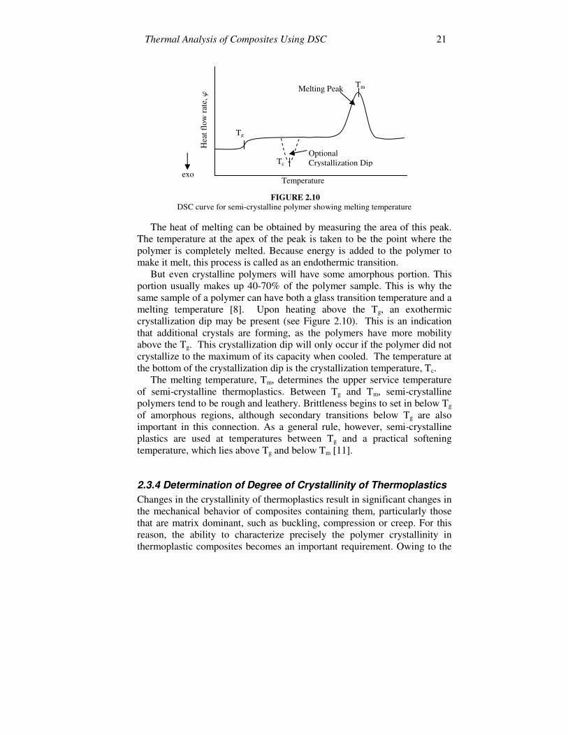
2.3.3 Determination of Melting Temperature (Tm) Melting is a transition which occurs in thermoplastic semi-crystalline polymers such as PEEK, polypropylene, polyvinyl chloride, polystyrene, and polyphenylene sulphide used in composites. Melting happens when the polymer chains fall out of their crystal structures and become a disordered liquid [8]. When a crystalline polymer is heated, the temperature increases at a constant rate until it reaches its melting point. The temperature will hold steady for a while until the polymer has completely melted, even though the heating continues. All the energy added to the crystalline polymer at its melting point goes into melting, and none of it goes towards raising the temperature. This heat is called the latent heat of melting. Once the polymer has melted, the temperature begins to rise again, but now it rises at a slower rate. The molten polymer has a higher heat capacity than the solid crystalline polymer, so it can absorb more heat with a smaller increase in temperature. So when a crystalline polymer melts, it absorbs a certain amount of heat (the latent heat of melting) and it undergoes a change in its heat capacity. This is called a first-order transition [7]. This extra heat flow during melting shows up as a large endothermic melting peak in the DSC plot, as indicated in Figure 2.10.


FIGURE 2.10

DSC curve for semi-crystalline polymer showing melting temperature

The heat of melting can be obtained by measuring the area of this peak. The temperature at the apex of the peak is taken to be the point where the polymer is completely melted. Because energy is added to the polymer to make it melt, this process is called as an endothermic transition.

But even crystalline polymers will have some amorphous portion. This portion usually makes up 40-70% of the polymer sample. This is why the same sample of a polymer can have both a glass transition temperature and a melting temperature [8]. Upon heating above the Tg, an exothermic crystallization dip may be present (see Figure 2.10). This is an indication that additional crystals are forming, as the polymers have more mobility above the Tg. This crystallization dip will only occur if the polymer did not crystallize to the maximum of its capacity when cooled. The temperature at the bottom of the crystallization dip is the crystallization temperature, Tc.

The melting temperature, Tm, determines the upper service temperature of semi-crystalline thermoplastics. Between Tg and Tm, semi-crystalline polymers tend to be rough and leathery. Brittleness begins to set in below Tg of amorphous regions, although secondary transitions below Tg are also important in this connection. As a general rule, however, semi-crystalline plastics are used at temperatures between Tg and a practical softening temperature, which lies above Tg and below Tm [11].

2.3.4 Determination of Degree of Crystallinity of Thermoplastics Changes in the crystallinity of thermoplastics result in significant changes in the mechanical behavior of composites containing them, particularly those that are matrix dominant, such as buckling, compression or creep. For this reason, the ability to characterize precisely the polymer crystallinity in thermoplastic composites becomes an important requirement. Owing to the

exo

Hea

t flo

w ra

te, �

Temperature

Melting Peak

Optional Crystallization Dip

Tg

Tc

Tm


heterogeneous nature of the composite, determination of crystallinity becomes more complicated. DSC analysis provides the modifications necessary for precise application to thermoplastic composites [12].

The determination of the degree of crystallinity (DOC) by differential scanning calorimeter is an indirect method, with the actual parameter measured being the heat of fusion. There are two ways of finding the DOC by this method: the cooling mode and the heating mode [13].

There are two methods of studying the crystallization kinetics in the cooling mode. To induce isothermal crystallization, the tested sample is first heated above its melting temperature, and then rapidly quenched to the prescribed crystallization temperature so that crystallization occurs isothermally. In non-isothermal crystallization, the tested sample is first heated to a prescribed temperature above its melting point, and then cooled at a preset cooling rate. The DOC is calculated from the heat of crystallization evolved during either process.

In the heating mode, a sample is heated up from ambient temperature in the DSC at a preset rate until it reaches its melting point. The DOC of the sample is then calculated by comparing the heat of fusion obtained for the tested sample with that of a reference sample with 100% DOC. The DOC obtained in the heating mode will differ from that obtained by the cooling mode.

At present there is no consensus as to which mode gives the true DOC of the sample. In any case, whichever mode is used, it has been pointed out that DSC does recrystallize the test sample (especially if it is highly amorphous) during the dynamic scan, and produces a higher than actual DOC. The degree of crystallinity is calculated by computing the net heats of fusion and crystallization over the range of the DSC scan. For an amorphous material or one of low DOC, recrystallization is inevitable during the scan. It is thus necessary to subtract this exothermic heat of crystallization from the total heat of fusion. In the case of highly crystalline material, there will be a secondary endothermic heat of reaction if it goes through an annealing process. The DOC can be calculated from the following equations: [13]

%100% ×∆

∆+∆=

f

cmH

HHDOC (2.9)

%100% ×∆

∆+∆=

f

amH

HHDOC (2.11)

In the above equations, Hm is the heat of fusion (endothermic); Hc is the

heat of cold-crystallization (exothermic); Ha is the premelt heat of crystallization (endothermic), which corresponds to the secondary


crystallization phase of the structure; and Hf corresponds to the heat of fusion for a 100% crystalline material.

The above equations are valid for virgin or unfilled materials (i.e., without reinforcement). The equations must be modified if they are to be used for fiber-reinforced composites. If Wf is the weight fraction of fiber content in a composite, then the 100% heat of fusion for this composite becomes Hf (1-Wf). Equations (2.9) and (2.11) then become:

%100)1(

% ×−∆∆+∆

=ff

cmWHHH

DOC (2.12)

and

%100)1(

% ×−∆∆+∆

=ff

amWHHH

DOC (2.13).

2.3.5 Characterization of Thermosets using DSC DSC is a valuable analytical tool for the analysis and characterization of thermosetting materials, such as epoxies, polyesters, and bismaleimides. Thermosetting materials are those which existed in an unreacted or partially reacted state and which underwent crosslinking after mixing the base components or heating to elevated temperatures. The properties of thermosetting materials are very much dependent upon their chemical formulation or composition along with the conditions (e.g., time and temperature) to which the resins are exposed during processing. Small changes in the formulation or processing conditions, which can effect the curing of the resins, can significantly affect the properties of the end product. The use of thermal characterization studies on thermosetting resin materials will avoid production problems and will be useful for troubleshooting purposes [14].

A thermosetting resin undergoes an irreversible chemical reaction during curing. As the components of the resin system cure, heat is evolved by the resin, which is monitored by DSC. Figure 2.11 represent the changes taking place during crosslinking. These changes can be readily observed by DSC [15].


uncured partially cured totally cured

FIGURE 2.11 Representation of increase in crosslink density of a thermosetting material, Ref [17] Figure 2.12 shows typical DSC results obtained by heating an uncured

thermosetting resin system at a constant rate.

FIGURE 2.12

DSC results for an uncured thermosetting resin

The curing is observed as a large exothermic peak. The onset of cure is the temperature at which heat flow deviates from a linear response, and the exothermic peak temperature reflects the maximum rate of curing of resin. At the completion of curing or crosslinking, the DSC heat flow returns to a quasi-linear response. The area under the exothermic peak can be integrated to give the heat of cure, (�Hcure-J/g).

As the thermosetting resin cures or crosslinks, the Tg increases and heat of cure decreases. These changes in Tg and heat of cure can be used to characterize and quantify the degree of cure of the resin system, which is given in equation (2.14) as [16]:

RHtH )(=α (2.14)

exo

Hea

t flo

w ra

te, �

Temperature

Exothermic Cure

Tg


where H(t) is the heat of cure up to time t and HR is the total heat of cure (or enthalpy of reaction). The degree of cure, �, ranges from zero (uncured) to unity (fully cured).

As the resin system approaches complete cure, the Tg will achieve a maximum value, Tg ( ∞ ), which is indicated in Figure 2.13 below:

FIGURE 2.13

DSC curves showing increase in Tg as a function of cure for a thermosetting resin, Ref [17]

The increase in Tg, observed as a function of the degree of cure, represents an increase in the cross link density of the resin system. The actual value of the Tg ( ∞ ) is dependent upon the chemical make-up of the particular resin system. The increase in Tg with regards to cure time is shown in Figure 2.14 for a given thermosetting resin system:

More Cured

Less Cured

Temperature

Hea

t flo

w ra

te, �

exo


FIGURE 2.14

Increase in Tg with cure time at a constant temperature for thermosetting resin, Ref [17]

As the resin becomes more crosslinked, the residual heat of curing becomes increasingly smaller, and as the material becomes completely cured, the heat of cure becomes undetectable. This phenomenon is illustrated in Figure 2.15, where samples of increasing degrees of cure are analyzed using DSC:

FIGURE 2.15

Decrease in residual cure exotherm for thermosetting resin with increasing cure levels, Ref [17]

The residual heat of cure may be used to determine the degree of cure of

the material, given by the ratio of the residual heat of cure to the heat of cure

Less Cured

More Cured

Temperature

Completely Cured

Hea

t flo

w ra

te, �

Cure Time

Gla

ss T

rans

ition

Tem

pera

ture

, Tg


of uncured resin material [17]. If no heat of cure is observed, then the value of � is 100%, and it is assumed that the resin is completely cured. In reality the resin may still have some lingering residual cure, but the DSC is no longer sensitive enough to detect this. The degree of cure value is important for end products generated from thermosetting resins, as it is related to brittleness, impact resistance, long term stability, creep, solvent resistance and product integrity[18].

2.4 Kinetic analysis A good example of where a complete understanding of cure parameters can be cost effective is the exotherm of thick parts. Many resins have a fairly small temperature window in which the rate of reaction increases rapidly. A cure cycle is required that will not allow an excessive exotherm to degrade the material, but will complete the cure in a reasonable amount of time, with acceptable flow. A complete understanding of the cure kinetics can assist in establishing the cure cycle and the safety margin present. Generation of DSC data involves a significant amount of time and expense. Time can be compressed by cure modeling, with little additional cost. Many different cure parameters (time, temperature history) can be investigated within a short period of time. Once the candidate cure cycle has been entered, the model is run in a matter of seconds.

Cure cycle generation has been an iterative process in the past. Usually the first acceptable rather than an optimized cure is accepted because of the time and expense. For the same reasons, determination of which families of tools can be cured together has often been arbitrary. A cure model helps in making informed decisions about these types of issues. The primary advantage of cure modeling is that a complete understanding of the primary factors during cure can be realized, rather than a limited understanding from a series of data points. Cure modeling does not interrupt the ongoing production or testing activities, but supports them offline, quickly evaluating cures and answering “what if” questions [19].

In kinetic analysis, it is generally assumed that the rate of reaction can be described by two separable functions, K(T) and f(�), such that [16]

)()( ααfTK

dtd ⋅= (2.15)


where d�/dt is the rate of reaction, K(T) is the temperature-dependent rate constant, and f(�) corresponds to the reaction model. The temperature dependence of the reaction rate is described by the Arrhenius equation: [17]

��

��

� −⋅=

RTE

ATK exp)( (2.16)

where R is the universal gas constant, E is the activation energy, and A is the pre-exponential factor.

For experiments in which samples are heated at a constant rate, the explicit time dependence in equation (2.15) can be eliminated so that [16]

)(exp αβ

αf

RTEA

dTd ⋅�

�

��

� −⋅= (2.17)

where � = dT / dt is the heating rate.

The kinetic parameters (A and E) are obtained by a linear transformation of equation (2.17) so that:

RTEA

fdT

d−��

��

�=

βα

αln

)(ln (2.18)

This equation, which has the form y = a0+a1y, can be used to determine the optimal fit of the kinetic parameters by multiple linear regression. However, the form of f(�) must be chosen a priori. Typical reaction models for thermosetting polymers are second order, f(�) = (1-�)2; nth order, f(�) = (1-�)n; and autocatalytic, f(�) = (1-�)n �m [16].

A relatively new approach to kinetic modeling is the model-free isoconversional method. This method assumes that both the activation energy and pre-exponential factor are not constants, but functions of the degree of cure [20]. The isoconversional approach can be used to evaluate both simple and complex chemical reactions. For the evaluation of data with this method, no kinetic rate expression is assumed a priori.

2.5 Modes of Operation DSCs are operated by a controlled program which changes the temperature in time. We distinguish between those modes of operation that leave the heating rate constant (i. e., the classical DSC operation mode) and those with variable (periodical or non-periodical) change of the heating rate.


2.5.1 Constant Heating Rate In the constant heating rate mode of operation, the sample temperature is controlled by the following relation [5]:

T(t)=To +�0�t (2.19)

where To is the starting temperature of the run and �0 is the heating or cooling (negative) rate. In other words, the temperature changes linearly in time.

A special case is the isothermal mode, in which the heating rate (�0 in equation 2.19) is zero, i.e., the temperature To is kept constant. Consequently, if no transitions or reactions take place in the sample, there is no heat exchanged with the sample and the heat flow rate should read zero. In practice this is not the case, as all DSC systems are not perfectly symmet-ric, and the heat exchange of the sample and reference sample with the sur-roundings is somewhat different. This results in a non-zero heat flow rate, even in the isothermal case. One reason to perform isothermal measurements in a DSC is to measure and check this asymmetry. Isotherms are used for calculation of heat flow rate corrections due to asymmetries. They are included before and after scanning sections in the case of precise heat capacity measurements. Another reason to perform isothermal measurements is to determine the latent heat of reactions or transitions taking place in the sample at a certain temperature. Of course, the baseline (the isotherm obtained without processes of the sample) must be subtracted from the measured curve to get the true reaction heat flow rate.

In the non-isothermal constant heating rate mode, the temperature changes linearly in time. In a DSC the differential heat flow rate depends on the differential heat capacity and heating rate as given by equation 2.20 [5]

dtdT

CpC p=ϕ (2.20)

Generally, the measured heat flow rate in scanning mode is never zero and is made up of three parts:

�(T, t) = �0(T) + �Cp(T) + �r(T, t) (2.21)

The first term on the right hand side is caused by the unavoidable asymmetry of the DSC; the second term is caused by the difference in heat capacity of the sample and reference sample; and the third term is the heat flow contribution from a reaction or transition (latent heat) occurring in the sample. The first two parts define the "baseline" and the third part the


"peak" of the measured curve. Scanning is the most commonly used mode of operation with DSC.

2.5.2 Modulated DSC (MDSC) The technique of modulated DSC was commercialized by TA Instruments in 1992. Instead of using a single linear heating rate, as used in traditional DSC, it employs a modulated or sinusoidal change in heating rate in order to automatically separate the heat capacity baseline from the total heat flow signal. This means that it is possible to identify, measure, and quantify kinetic processes in a single experiment. The heat flow signal is composed of several parts, but traditional DSC can only measure the sum of those parts and illustrate the sum in a single signal. With MDSC, multiple signals are generated in a single experiment so that each of the components to the total heat flow signal can be shown and analyzed independently [21,22].

In the variable heating rate operation, a certain modulation term is added to the linear part of the temperature-time function. The simplest and most frequently used modulation type is the periodic (sinusoidal) type governed by equation 2.22 [5]:

T(t) =T0 + �0�t + TA�sin(�t) (2.22)

where TA is the amplitude and � is the angular frequency of the modulation. Together with �0, the "underlying" heating rate, there are three parameters that can be chosen freely within certain limits. This influences the heating rate, which follows from Equation (2.22) as:

dT/dt = �o + TA��cos(�t) (2.23)

Depending on the relation of �o to TA �, we can distinguish four cases: quasi-isothermal, heating-cooling, heating only, and heating-iso [5].

In the quasi-isothermal mode of operation, the underlying heating rate is zero and the temperature varies around a constant temperature. As the amplitude of the modulation is low (0.01 to 0.5 K normally), the temperature is almost constant. The heating/cooling rate varies between ±TA �. The advantage of using this mode is the possibility to determine heat capacities, even in the isothermal case, which otherwise is not possible.

In the heating-cooling mode, the amplitude is so large with respect to �o that the heating rate changes its sign periodically, i. e., the sample is periodically heated and cooled. This is the case if the product TA � is


larger than the underlying heating rate �o. The advantage of this mode is the rather large heating rate and subsequent good signal-to-noise ratio, which is in particular useful if we have small sample masses. The disadvantage is that the sample is heated and cooled during the run, which may cause problems in some cases, e.g., for polymers where different processes (with different time constants) could occur within the heating and cooling period. This would complicate the evaluation of the processes.

For the heating-only mode, the amplitude is so small that the heating rate is always positive, i.e. the sample is only heated and never cooled dur-ing a run. This is the case if the product TA � is smaller than the underlying heating rate �o. The advantage of this mode is that all processes which only occur during cooling of the sample are suppressed, and the remaining processes are easier to evaluate. The disadvantage is the bad signal-to-noise ratio for all quantities derived from it.

The heating-iso mode is the limiting case between the two modes above, where TA �=�o. The heating rate varies periodically between TA �+�o and zero. This mode has the maximum signal-to-noise ratio but without cooling the sample.

2.6 Conclusion DSC thermal analysis is an important tool in the experimental characterization of composite materials. It is used to evaluate polymers and polymer matrix composites for diverse applications such as automobiles, aircrafts, space vehicles, containers, and piping systems for the marine and petrochemical industries [15,17]. DSC equipment and modes of operation vary from heat flux DSC to power compensated DSC and constant heating rate DSC to modulated DSC. Fundamentally the DSC measures the heat capacity of a sample by recording the heat flow rate into the sample and comparing it to a reference sample. From the DSC curve one can determine materials transition points such as the glass transition temperature and melting temperature. The DSC can also quantify the degree of crystallinity for thermoplastic matrices and the residual heat of reaction for thermosetting resins. Additionally, the curing characteristics of thermosetting matrices can be modeled from limited DSC curves to develop a mathematical cure kinetic model that can be used for process optimization and curing simulations.


References 1. T. Hatakeyama and F.X. Quinn, Thermal Analysis : Fundamentals and

Applications to PolymerScience, Chichester [England] ; New York John Wiley & Sons, Ltd.(UK), 1999.

2. J.M. Barton, The Application of Differential Scanning Calorimetry (DSC) to the Study of Epoxy Resins Curing Reactions. Vol. 72, pp. 111-154. (04/06/2004)

3. G. Dallas, Thermal Analysis, ASM Handbook – Composites, ASM International, Vol. 21, pp. 973-976, Materials Park, OH, 2001.

4. P.J.Haines, Thermal Methods of Analysis, London New York Blackie Academic & Professional 1995 1st ed (P973-976) (04/02/2004)

5. G.H. Hohne, W.F. Hemminger, and H.J. Flammersheim, Differential Scanning Calorimetry, Springer Publishers (Engineering Index, 02/06/2004)

6. Cornerstone Research Group, Inc. Online. Internet. May 2, 2004 <http://www.crgrp.net/dsc.htm>

7. Department of Polymer Science, University of Southern Mississippi. Online. May 2, 2004 <http://www.psrc.usm.edu/macrog/dsc.htm>

8. Department of Polymer Science, University of Southern Mississippi. Online. May 2, 2004 <http://www.psrc.usm.edu/macrog/tg.htm>

9. University of Missouri – Columbia. Online. May 2, 2004 <http://www.missouri.edu/~crrwww/katti/Thermal%20Behavior%20of %20Polymers.pdf>

10. ASTM E1356-03 Standard Test Method for Assignment of the Glass Transition Temperatures by Differential Scanning Calorimetry, Annual Book of ASTM standards, Vol 09.01.

11. A. Rudin, Elements of Polymer Science and Engineering, Introductory Text and Reference for Engineers and Chemists

12. C.J. Wolf and J.A. Bornmann, Differential Scanning Calorimetry (DSC) to Determine Crystallinity in Poly (aryl-ether-ether-ketone) PEEK, National SAMPE Symposium and Exhibition (Proceedings), v 35, n pt 2, Apr, 1990, p 1167-1172.

13. T.H. Lee, F.Y.C. Boey and K.A. Khor, On the determination of polymer crystallinity for a thermoplastic PPS composite by thermal analysis, Composites Science and Technology, v 53, n 3, 1995, p 259-274 (11/22/94)

14. D.J. Plazek and Z.N. Frund Jr., Epoxy Resins (DGEBA): The Curing and Physical Aging process, Journal of Polymer Science, Part B: Polymer Physics, v 28, n 4, Mar, 1990, p 431-448.

15. Y.I. Xiao-Su, Matrix resin improvement for aerospace polymer matrix composites, 46th International SAMPE Symposium, May 6-10, 2001.

16. M.R. Kessler, S.R. White, Cure Kinetics of the Ring-Opening Metathesis Polymerization of Dicylcopentadine, Journal of Polymer Science A: Polymer Chemistr.y 2002; 40 2373-2383.


17. W.J. Sichina, Characterization of Epoxy Resins Using DSC, Perkin Elmer

Instruments. Online <http://las.perkinelmer.com/content/ApplicationNotes/TA%20PETech-70.PDF>

18. J.W. Chin, T. Nguyen, and K. Aouadi, Effects of environmental exposure on Fiber-Reinforced Plastic (FRP) materials used in Construction, ASTM, 1997.

19. E. Bryant, Crosslink density and glass transition in thermosetting polymers. Online. May 2, 2004 <http://www.udri.udayton.edu/rpdl/Paper_CROSDENS/Paper.htm>

20. S. Vyazovkin, A unified approach to kinetic processing of nonisothermal data (1996), John Wiley and Sons, Inc.

21. L.C.Thomas, Use of multiple heating rate DSC and modulated temperature DSC to detect and analyze temperature-time-dependant transitions in materials, January 2001 <http://www.iscpubs.com/articles/al/a0101tho.pdf>

22. R.B Prime, Vol 2, E.A.Turi, Ed., Academic Press, 1997, chap.6, Thermal characterization of polymeric materials

Thermal Analysis of Composites Using DSC · Thermal Analysis of Composites Using DSC by Suchitra...

Documents

Transcript of Thermal Analysis of Composites Using DSC · Thermal Analysis of Composites Using DSC by Suchitra...