THEORY OF r~IXED AND HYBRID FINITE-ELEMENTAPPROXIMATIONS IN LINEAR ELASTICITY

J. T. ODEN and J. K. LEE

IUTAMjIUM Symposium on Applications of Methods ofFunctional Analysis to Problems of Mechanics

Marseille, FranceSeptember, 1975

To be published by Springer-Verlag, Berlin, Heidelberg, and New Yorkin the series Lecture Notes in Mathematics.

THEORY OF MIXED AND HYBRID FINITE-ELEMENTAPPROXIMATIONS IN LINEAR ELASTICITY

J. T. ODEN and J. K. LEE

Texas Institute for Computational MechanicsThe University of Texas, Austin

1. Introduction

The complementary and dual variational principles of solid mechanics have alwaysoccupied an important place in elasticity theory, not only because they representsomething intermediate to the classical extremal principles of potential and comple-mentary energy, but also because they form the basis for a variety of effective me-thods of approximation. The well-known method of the hypercircle of Prager and Synge[1] is, in fact, rooted in these principles, as are the popular mixed finite-elementmethods, introduced by Hermann [2] and based on Reissner's principle [3]. In recentyears, there has been added to this collection of ideas a new family of special varia-tional methods referred to as hybrid methods. These have been largely developed byPian and his associates (e.g. [4]) in connection with finite element approximationsin solid and continuum mechanics. A summary of these variational concepts, togetherwith some discussion of their mathematical properties, can be found in the book ofOden and Reddy [5].

While the mixed and hybrid finite element methods have proved to be very effec-tive in certain specific numerical experiments, they also frequently meet with dis-appointing and often unexplained failure. For example, it is not uncommon to con-struct apparently reasonable approximations of stress and displacement fields in afinite element, only to find that they lead to singular or ill-conditioned stiffnessmatrices. The mathematical properties of mixed models which are responsible for theirdelicate behavior were examined in the papers of Oden and Reddy [6,7], Ciarlet andRaviart [8], and Johnson [9] for model second- and fourth-order problems. The theoryof hybrid methods is considerably more involved. Certain properties of a class ofhybrid methods are discussed in the reports of Raviart [10] and Thomas [11], and afairly detailed theory of mixed-hybrid methods for the solution of a model second-order problem has been contributed recently by Babuska, Oden, and Lee [12].

In the present paper, we present a theory of mixed a~d of hybrid finite elementapproximations of a class of problems in linear plane elasticity. Our treatment of

(2.2)

2

mixed methods generalizes all of those published previously and our method of proofdiffers considerably from others. Our principal tools are two fundamental theoremsdue to Babuska [13] (see also [14], [15]), one which generalizes the well-known lax-Milgram theorem and another which establishes bounds for the approximate problem.After introducing some aspects of the general theory of mixed variational principlesin Section 2 of the paper and describing a class of linear elastostatic problemswith a collection of pertinent notations in Section 3, we prove, in the fourth sec-tion, an existence theorem for the corresponding mixed variational problem. A theoryof mixed finite elements is given in Section 5. There we present sufficient condi-tions for the existence of unique solutions to the approximate problem, convergencecriteria, and a-priori error estimates. We are also able to develop, apparently forthe first time, l2-error estimates for mixed finite element approximations. In Sec-tion 6 we construct a special "hybrid" variational principle for plane elasticityproblems as well as a corresponding existence theorem. We demonstrate in Section 7that the hybrid principle leads naturally to a theory for "displacement" hybridfinite element approximations in which triangular elements are used, the displacementfield is approximated on the interior of the elements, and boundary tractions areapproximated on the element boundaries. Here we also give conditions for the exis-tence of approximate solutions as well as a-priori error estimates.

2. General Theory of Mixed Variational Principles

A fairly complete account of the general; theory of mixed (dual and complementary)variational principlas for l'lnear problems in mathematical physics is given in thebook of Oden and Reddy [5]. There it is shown that the functional

J(U,E,O) : -21<E€,E) + (o,Tu - €) - (f,u)G G H

+ (0 o,bu - gl) - (g2'Y u) (2.1)o aG 0 aH1 2

assumes a stationary value whenever the triple (U,E,O) satisfies the equations

Tu : E } bu : 91 on anl }

E€ = 0 in nT*o = f b* = g2 on an2

where H, G, aGl, and aH2 are function spaces defined on the doma~n nc ~n and boun-dary segments anl and an2, H is densely imbedded in G, ("')(.) denotes the dualitypairing on the underlying space (.), Yo: H + aH2 and 00: G + aGl are trace operators(continuous extensions), T is a continuous linear map of H into G. T* is its formaladjoint, band b* are boundary operators, f, gl' and 92 denote data, and E isa canonical isomorphism of G onto its dual G1

•

The relationship between the abstract problem (2.2) and the linear elasticity

3

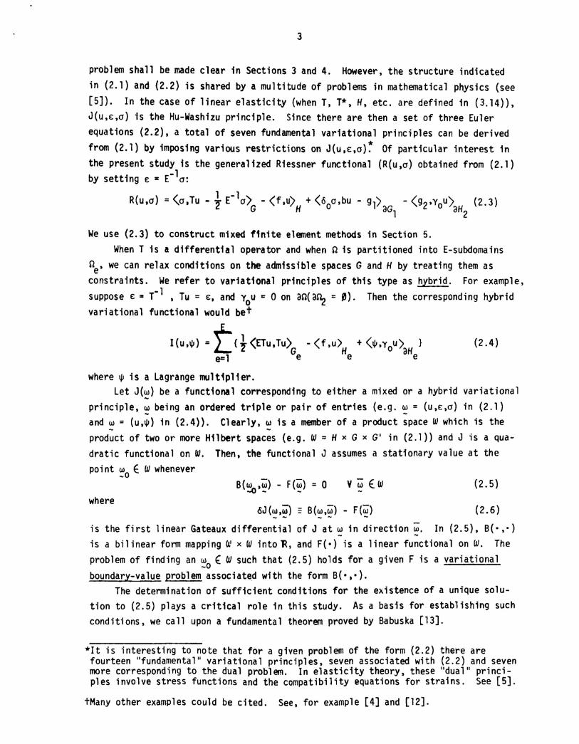
problem shall be made clear in Sections 3 and 4. However, the structure indicatedin (2.1) and (2.2) is shared by a multitude of problems in mathematical physics (see[5]). In the case of linear elasticity (when T, T*. H, etc. are defined in (3.14)),J(U,E,O) is the Hu-Washizu principle. Since there are then a set of three Eulerequations (2.2), a total of seven fundamental variational principles can be derivedfrom (2.1) by imposing various restrictions on J(U.E,O)~ Of particular interest inthe present study is the generalized Riessner functional (R(u,o) obtained from (2.1)by setting E = E-lo:

R(u,o) = (o.Tu - t £-10) - (f.u) + (ooo,bu - gl) - (gZ'you) (2.3)G H aGl 13HZ

We use (2.3) to construct mixed f1nite element methods in Section 5.When T is a differential operator and when n is partitioned into E-subdomains

ne' we can relax conditions on the admissible spaces G and H by treating them asconstraints. We refer to variational principles of this type as hybrid. For example,suppose E = T-l , Tu : E. and You = 0 on an(anz : 0). Then the corresponding hybridvariational functional would bet

I (u.~) =t{l(ETu.Tu) - (f .u) + (~.you> ) (2.4)e=l Ge He aHe

where ~ is a lagrange multiplier.Let J(~) be a functional corresponding to either a mixed or a hybrid variational

principle, ~ being an ordered triple or pair of entries (e.g. ~: (U.E.O) in (2.1)and w = (u,~) in (2.4)). Clearly, w is a member of a product space W which is the- -product of two or more Hilbert spaces (e.g. W : H x G X G' in (2.1)) and J is a qua-dratic functional on W. Then, the functional J assumes a stationary value at thepoint w E W whenever_0

where

VwEw (2.5)

oJ(w,W) = B(w,w) - F(w) (2.6)-- -- -is the first linear Gateaux differential of J at ~ in direction~. In (2.5), B(·,·)is a bilinear form mapping W x W into~. and F(') is a linear functional on W. Theproblem of finding an w f W such that (2.5) holds for a given F is a variational

-0boundary-value problem associated with the form B(·,·).

The determination of sufficient conditions for the existence of a unique solu-tion to (2.5) plays a critical role in this study. As a basis for establishing suchconditions, we call upon a fundamental theorem proved by Babuska [13].

*It is interesting to note that for a given problem of the form (2.2) there arefourteen "fundamental" variational principles, seven associated with (2.2) and sevenmore corresponding to the dual problem. In elasticity theory, these "dual" princi-ples involve stress functions and the compatibility equations for strains. See [5].

tMany other examples could be cited. See, for example [4] and [12].

4

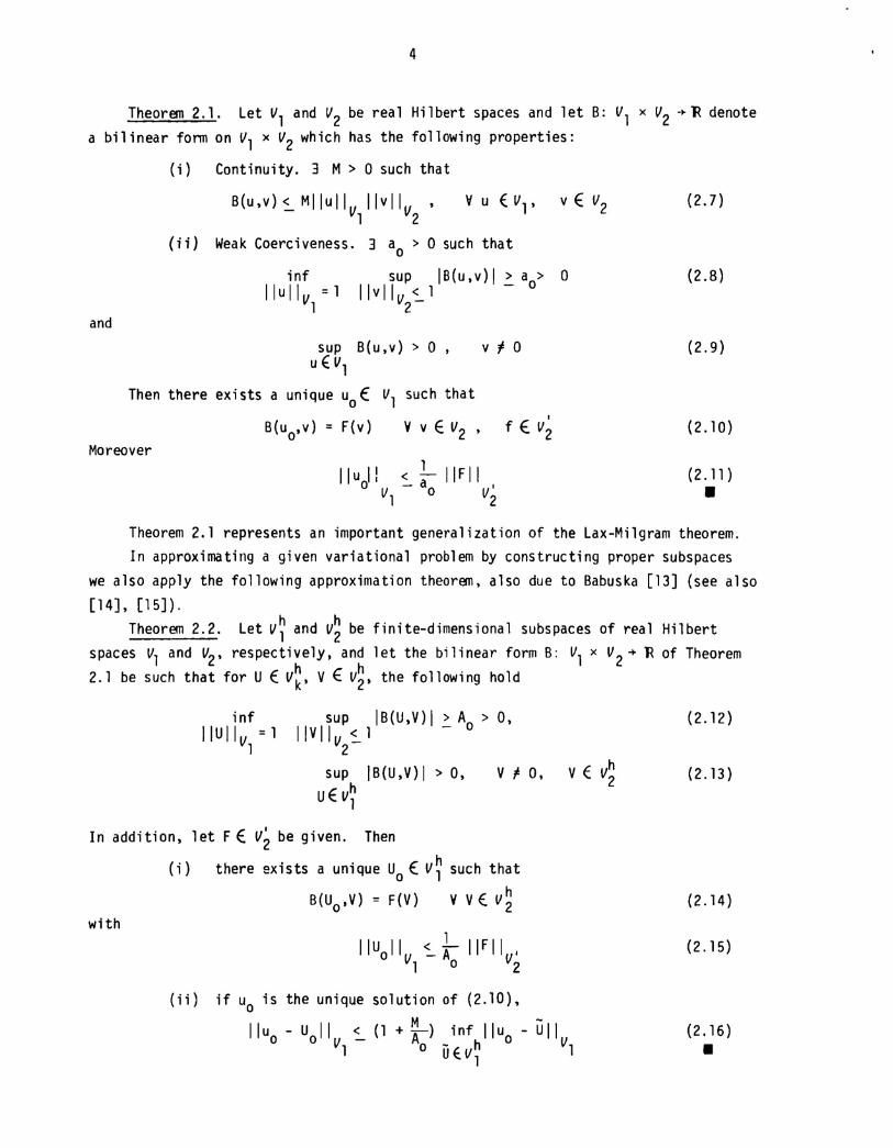
Theorem 2.1. Let Vl and V2 be real Hilbert spaces and let B: Vl x V2 +~ denotea bilinear form on Vl x V2 which has the following properties:

(i) Continuity. 3 M > 0 such that

Vu(Vl, vEV2 (2.7)

and

(ii) Weak Coerciveness. 3 ao > 0 such that

inf sup IB(u,v)1 > ao> 0Iluliv =1 Ilvllv~l -

1 2

(2.B)

sup B(u,v) > 0 ,u E Vl

Then there ex; sts a unique Uo E Vl such that

v 'I 0 (2.9)

v v E V2• f E V~ (2.10)Moreover

1Ilu I! < a IIFII

o v - 0 v'1 2

(2.11)

•Theorem 2.1 represents an important generalization of the lax-Milgram theorem.In approximating a given variational problem by constructing proper subs paces

we also apply the following approximation theorem, also due to Babuska [13] (see also[14], [15]).

Theorem 2.2. let V~ and V~ be finite-dimensional subspaces of real Hilbertspaces Vl and V2' respectively, and let the bilinear form B: Vl x V2+ R of Theorem2.1 be such that for U E V~, V E V~, the following hold

infIlu II V = 1

1

sup IB(U,V)I > Ao > 0,IIVllv ~l -

2

(2.12)

sup IB(U,V)I > 0,uE Vh

1

V "I O. (2.13)

In addition, let F E V~ be given. Then

(i) there exists a unique Uo E V~ such that

B(Uo'V) = F(V) V V E V~with

IluollV ~}-IIFllv,1 0 2

(ii) if Uo is the unique solution of (2.10),M -Ilu - u II < (1 + A) inf Iluo - U II

o 0 vl - 0 - £. h vlU ~ V 1

(2.14)

(2.15)

(2.16)

•

5

(3.2)

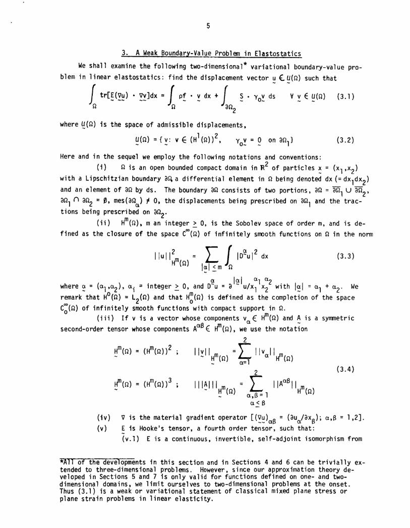
3. A Weak Boundary-Value Problem in Elastostatics

We shall examine the following two-dimensional* variational boundary-value pro-blem in linear elastostatics: find the displacement vector ~ ~~(n) such that

1 tr[~(y~) . y~]dx= 1 p! . ~ dx·1 ~. yo~ ds V ~ E ~(O) (3.1 )n n a02

where ~(n) is the space of admissible displacements,

~(n)={~:vE(Hl(!1))2, Yo~:~ onanl}

Here and in the sequel we employ the following notations and conventions:(i) n is an open bounded compact domain in R2 of particles ~ = (xl,x2)

with a Lipschitzian boundary a~ a differential element in n being denoted dx (=dxldx2)and an element of an by ds. The boundary an consists of two portions, an = anl LJ a02,anl n an2 : 0, mes(ana) ; 0, the displacements being prescribed on anl and the trac-tions being prescribed on a02.

(ii) Hm(O), m an integer ~ 0, is the Sobolev space of order m, and is de-fined as the closure of the space C~(o)of infinitely smooth functions on 0 in the norm

(3.3)

(3.4)

IIul12m = [l10~u12 dxH (0) 1~I2.m 0

alai al a2where ~ : (al,a2), ai = integer ~ 0, and O-u = a - u/xl x2 with I~I = al + a2. Weremark that HO(n) = L2(n) and that H~(O) is defined as the completion of the spaceC~(n) of infinitely smooth functions with compact support in n.

(iii) If v is a vector whose components v E Hm(n) and A is a symmetricB a -

second-order tensor whose components Aa E ~(o), we use the notation2

Ilvll m ) = \ IIvall m )- ~ (n ~ H (n

2

III ~III m ( ) = L II A aB II m( )H n a,B = 1 H n

a<B

(i v)(v)

~ is the material gradient operator [(Vu) 0 = (au /axo); a,B = 1,2].-- aµ a µ

E is Hooke's tensor, a fourth order tensor, such that:(v.l) E is a continuous, invertible, self-adjoint isomorphism from

*All of the developments in this section and in Sections 4 and 6 can be trivially ex-tended to three-dimensional problems. However, since our approximation theory de-veloped in Sections 5 and 7 is only valid for functions defined on one- and two-dimensional domains, we limit ourselves to two-dimensional problems at the onset.Thus (3.1) is a weak or variational statement of classical mixed plane stress orplane strain problems in linear elasticity.

6

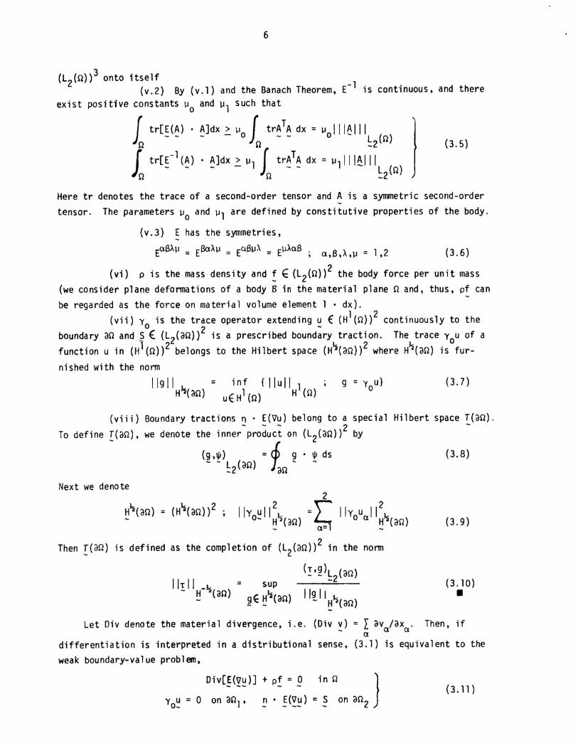
(l2(n))3 onto itself(v.2) By (v.l) and the Banach Theorem, E-l is continuous, and there

exist positive constants µo and µl such that

J tr[E(A)· A]dx~µ f trATAdx: µ IIIAIIIn - - - 0 n - - 0 -~2(n) ~ (3.5)

1tr[E-l (A) . A]dx ~ µl f trATA dx = µ11l1~111- - - - - l (n)n n _2

Here tr denotes the trace of a second-order tensor and A is a symmetric second-ordertensor. The parameters µo and µl are defined by constitutive properties of the body.

(v.3) E has the symmetries,

EoBAµ = EBaAµ = EaBµ\ : EµAoB; O,B,A,µ: 1.2 (3.6)

(vi) p is the mass density and! E (l2(n))2 the body force per unit mass(we consider plane deformations of a body B in the material plane n and, thus, pf canbe regarded as the force on material volume element 1 . dx).

(vii) y is the trace operator extending u E (Hl(n))2 continuously to theboundary an and SOE (L2(an)2 is a prescribed bound~ry traction. The trace You of afunction u in (H1(n))2 belongs to the Hilbert space (H~(an))2 where H~(an) is fur-

nished with the norm

Ilgli Js = inf {llulllH (an) uE H1(n) H (n)

g = You} (3.7)

(viii) Boundary tractions n . E(Vu) belong to a special Hilbert space T(an).- - - 2 -

To define I(an). we denote the inner product on (L2(an)) by

(g.l/J) : rr; g' IjJ ds (3.8)- - L (an) 1: - -

-2 anNext we denote

= supII!II H-~(an) gE H~(an)- - -

Then T(an) is defined as

22 L 2Ily u II = lIy u II

0- H~(dn) 0:1 0 0 HJs(an)

the completion of (l2(an))2 in the norm

(!'2\2(an)

Ilg II- H~(an)

(3.9)

(3.10)•Let Oiv denote the material divergence, i.e. (Div v) = L av lax. Then, if

- 0 0odifferentiation is interpreted in a distributional sense, (3.1) is equivalent to theweak boundary-value problem,

Div[E(Vu)] + pf = 0 in n }

yo~ = 0 on anl, ~. 5(~~)c ~ on an2(3.11)

7

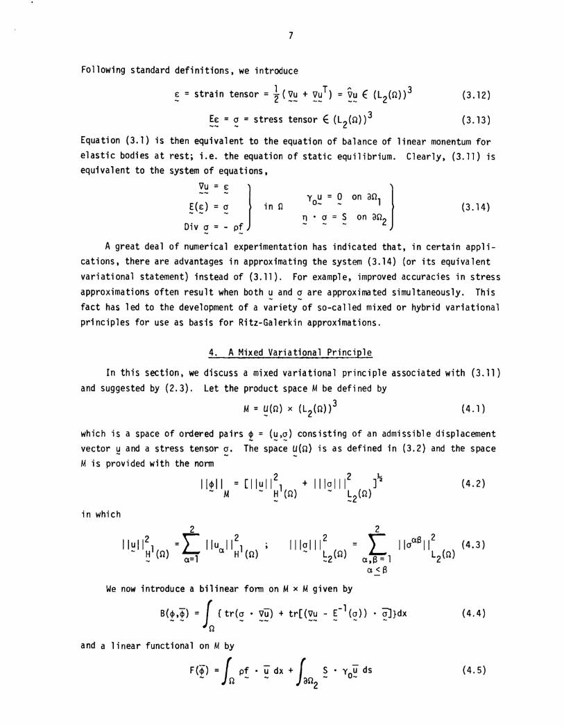
Following standard definitions, we introduce

.: = strain tensor : ~ (~~ + ~~T) = ~~ E (l2(n))3

~.:: ~ : stress tensor E (l2(n»)3

(3.12)

(3.13 )

(3.14)yo~ = ~ on anl }

~ • ~ = ~ on an2

Equation (3.1) is then equivalent to the equation of balance of linear monentum forelastic bodies at rest; i.e. the equation of static equilibrium. Clearly. (3.11) isequivalent to the system of equations,

Vu = E 1~(.:) = ~ in n

D1V 0 = - pf

A great deal of numerical experimentation has indicated that, in certain appli-cations, there are advantages in approximating the system (3.14) (or its equivalentvariational statement) instead of (3.11). For example. improved accuracies in stressapproximations often result when both ~ and ~ are approximated simultaneously. Thisfact has led to the development of a variety of so-called mixed or hybrid variationalprinciples for use as basis for Ritz-Galerkin approximations.

4. A Mixed Variational Principle

In this section, we discuss a mixed variational principle associated with (3.11)and suggested by (2.3). let the product space M be defined by

M = ~(n) x (l2(n))3 (4.1)

which is a space of ordered pairs! = (~,~) consisting of an admissible displacementvector u and a stress tensor o. The space u(n) is as defined in (3.2) and the space- --M is provided with the norm

(4.2)

in which

2111~llll (n)

-2

2

La,S = 1

a<S

We now introduce a bilinear form on M x M given by

B(!,!) : f {tr(~ • ~~) + tr[(~~ - r 1(~)} • ~}dxn

(4.4)

and a linear functional on M by

F('$) : ( pf· u dx + f S· You ds- In - - an - -2

(4.5)

8

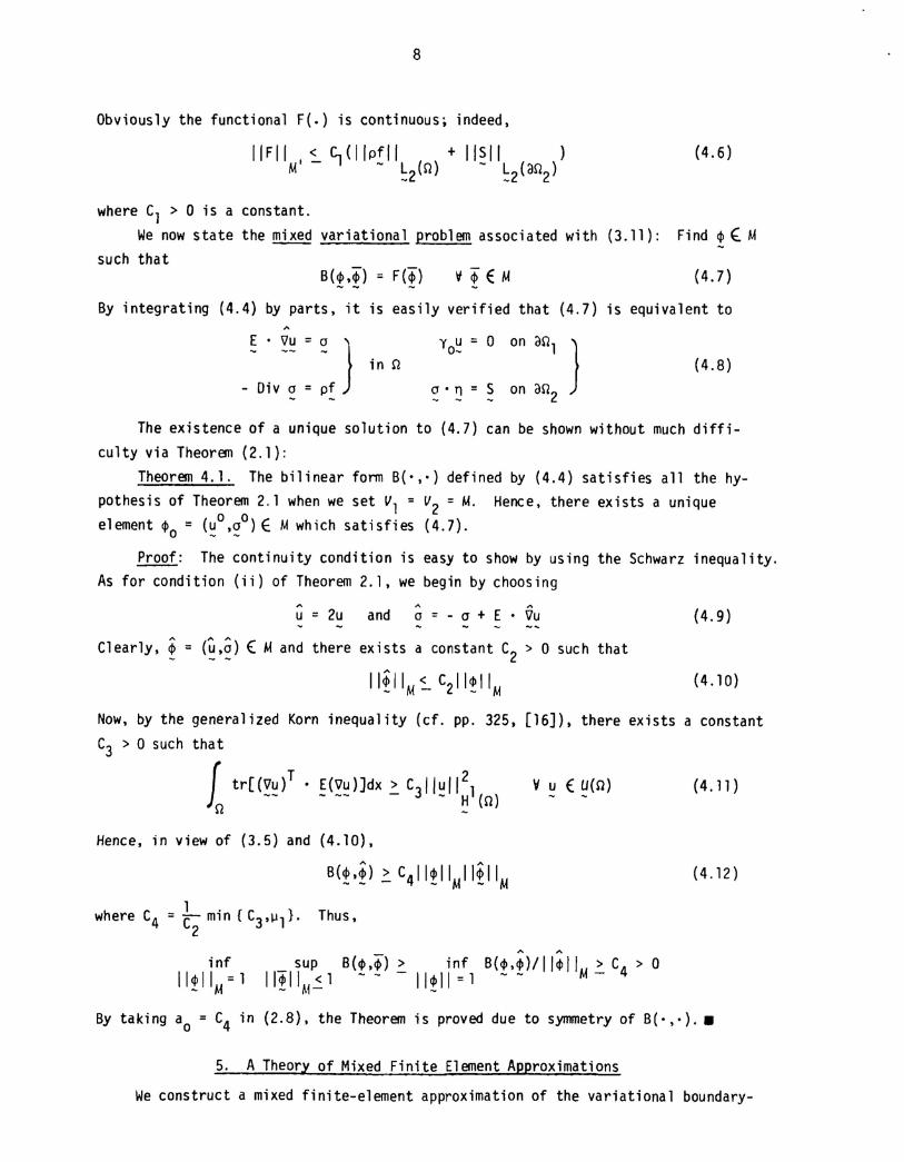
Obviously the functional F(.) is continuous; indeed,

IIFII < C_(llpfll +IISII) (4.6)M' - -I - l (n ) - l (an )_2 _2 2

where C1 > 0 is a constant.We now state the mixed variational problem associated with (3.11): Find ~ (M

such thatIf ~ EM (4.7)

By integrating (4.4) by parts, it is easily verified that (4.7) is equivalent to

y u = 0 on anl }0-

~ • ~ : ~ on arl2(4.8)

The existence of a unique solution to (4.7) can be shown without much diffi-culty via Theorem (2.1):

Theorem 4.1. The bilinear form B(·,·) defined by (4.4) satisfies all the hy-pothesis of Theorem 2.1 when we set Vl = V2 = M. Hence, there exists a uniqueelement ~o = (~o,~o) E M which satisfies (4.7).

Proof: The continuity condition is easy to show by using the Schwarz inequality.As for condition (ii) of Theorem 2.1, we begin by choosing

u = 2u and ~: - 0 + E • Vu~ - ~ - - -~

Clearly, ~ = (u,a) ( M and there exists a constant C2 > 0 such that

II~ IIM ~ C211~ II M

(4.9)

(4.10)

Now, by the generalized Korn inequality (cf. pp. 325, [16]), there exists a constantC3 > 0 such that

1 T 2tr[(Vu) • E(Vu)]dx > C31 lull 1-- - -- - - H (n)

n -Hence, in view of (3.5) and (4.10),

B(2'~) ~ C411~IIMII~IIM

where C4 = t- min {C3,lll}' Thus,2

VuE u(n) (4.11)

(4.12)

,.. ...inf B($,$)/ I/$IIM > C4 > 0

11~11=1 -- -

By taking ao = C4 in (2.8), the Theorem is proved due to symmetry of B(·,·) .•

5. A Theory of Mixed Finite Element Approximations

We construct a mixed finite-element approximation of the variational boundary-

9

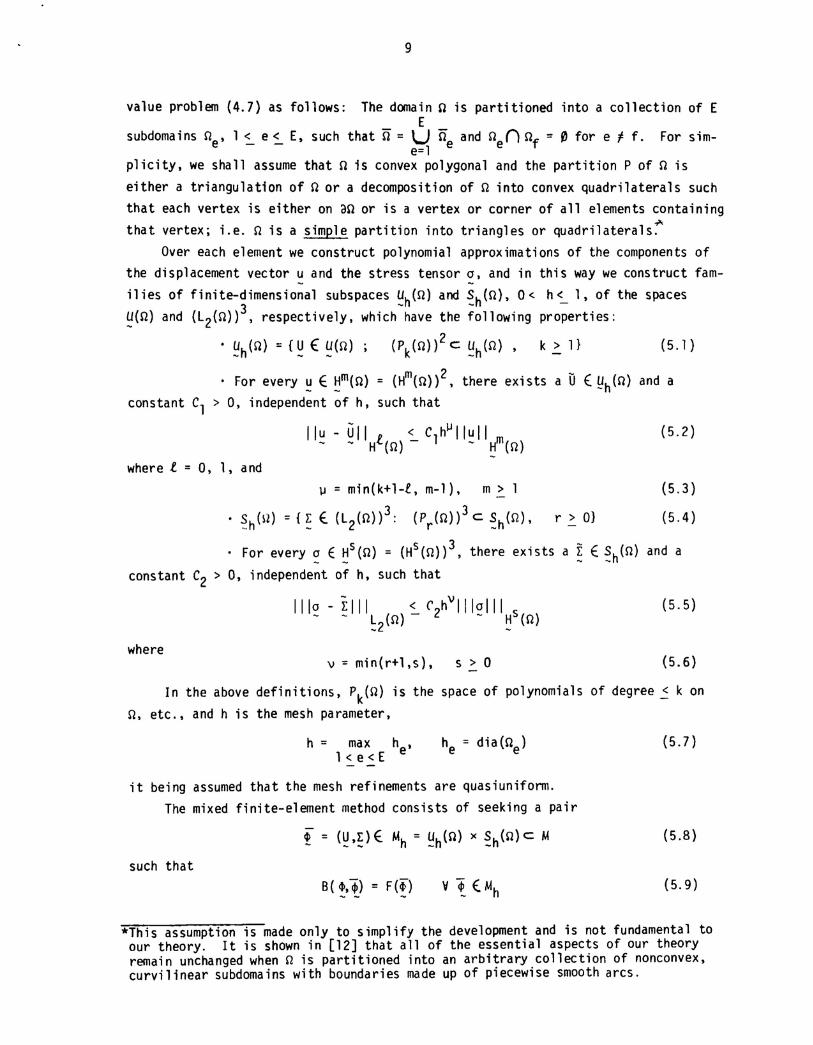
value problem (4.7) as follows: The domain n is partitioned into a collection of EE

subdomains net 1 < e < E, such that IT = U nand n n nf : £) for e t- f. For sim-- - e=l e e

plicity, we shall assume that n is convex polygonal and the partition P of n is

either a triangulation of n or a decomposition of n into convex quadrilaterals such

that each vertex is either on an or is a vertex or corner of all elements containing

that vertex; i.e. n is a simple partition into triangles or quadrilaterals:

Over each element we construct polynomial approximations of the components of

the displacement vector u and the stress tensor 0, and in this way we construct fam-- -ilies of finite-dimensional subs paces ~h(n) and ~h(n). 0< h~ 1, of the spaces

~(n) and (L2(n))3. respectively, which have the following properties:

• ~h(n) : {~E ~(n); (Pk(n))2c ~h(n). k> 1} (5.1)

m m 2 -For every ~ E ~ (n) = (H (n») • there exists a U (~h(n) and aconstant Cl > 0, independent of h, such that

where l = 0, 1, and

~ = min(k+l-i, m-l). m> 1

• ~h(l2) = {~E. (L2(n»)3: (Pr(n)3C ~h(n), r> O}

For every ~ E ~s(n) = (Hs(n)3, there exists a ~ E ~h(n)

constant C2 > O. independent of h, such that

1110 - i: III < C2h \) III 0 III s- - L (n) - - H (n)

-2where

\) = min(r+l,s). s > 0

(5.2)

(5.3)

(5.4)

and a

(5.5)

(5.6)

In the above definitions, Pk(n) is the space of polynomials of degree 2 k on

n. etc., and h is the mesh parameter,

h = max he'l<e<E

(5.7)

it being assumed that the mesh refinements are quasiuniform.

The mixed finite-element method consists of seeking a pair

such that

(5.8)

B( <1>,"$) : F(~) (5.9)

*This assumption is made only to Simplify the development and is not fundamental toour theory. It is shown in [12] that all of the essential aspects of our theoryremain unChanged when n is partitioned into an arbitrary collection of nonconvex.curvilinear subdomains with boundaries made up of piecewise smooth arcs.

(5.10)

10

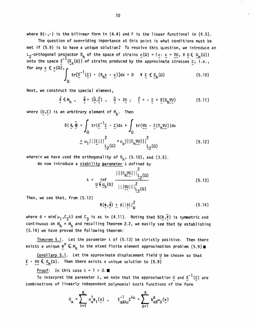
where B("') is the bilinear form in (4.4) and F is the linear functional in (4.5).The question of overriding importance at this point is what conditions must be

met if (5.9) is to have a unique solution? To resolve this question, we introduce an

L2-orthogonal pr~~ector TIhof the space of strains ~(~) : {~: ~ = ~~, V ~ E ~h(Q)}onto the space ~ (~h(~)) of strains produced by the approximate stresses ~; i.e.,for any £ ( £(~),- - f 1tr[~-(~) . (TIh: - ~)]dx= 0 V ~ E~h(n)

nNext, we construct the special element,

(5.11)

where (U,r) is an arbitrary element of Mh. Then

B( ~,~) = f tr(~-l~ • ~)dx + I tr(~~ • ~(TIh~~))dx~ ~

2 2~ µllil 1: II ! + µo IIIIThVUIII

- l (n) -- L (n)-2 -2

wherein we have used the orthogonality of ITh, (5.10), and (3.5).We now introduce a stability parameter A defined by

2IIITIh~~llll (0)

A = inf -2

~~~h(~) IIIvUII12

-- ~2(n)Then, we see that, from (5.12)

(5.12)

(5.13)

(5.14)

where B = mirnµl ,C3A} and C3 is as in (4.11). Noting that B(!,!) is symmetric andcontinuous on Mh x Mh and recalling Theorem 2.2, we easily see that by establishing(5.14) we have proved the following theorem:

Theorem 5.1. Let the parameter A of (5.13) be strictly positive. Then thereexists a unique !o (Mh to the mixed finite element approximation problem (5.9).

Corollary 5.1. Let the approximate displacement field ~ be chosen so thatE • ~~ (~h(n). Then there exists a unique solution to (5.9)

Proof: In this case A = 1 > 0 .•To interpret the parameter A, we note that the approximation ~ and ~-l(~) are

combinations of linearly independent polynomial basis functions of the form

KU : \ aicp.(x) ,(l L a 1 -

i:1

11

(5.14)

(5.15)

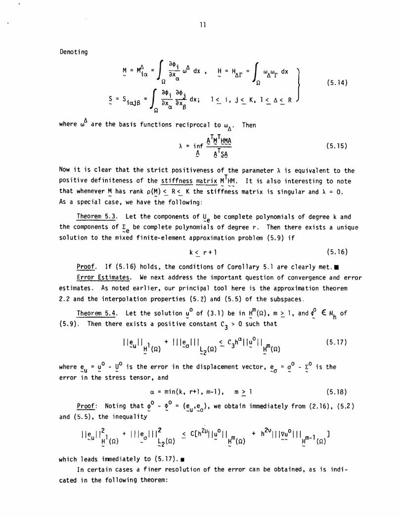
~ = H6r = 1Wl\Wr dx ]

l~i.j~K.nl<A<R

Denoting ../\ f a4li /).~ = M1a = ax- W dx ,n a

1 a4l. a4l.s = s. 'Q = ~ ~ dx;- laJI-' oX OXonap

where w/). are the basis functions reciprocal to w/).. Then

ATMTHMA). = inf - - ---

~ 8TS8

Now it is clear that the strict positiveness of the parameter). is equivalent to the

positive definiteness of the stiffness matrix MTHM. It is also interesting to note

that whenever ~ has rank p(~) ~ R~ K the stiffness matrix is singular and). = O.

As a special case, we have the following:

Theorem 5.3. Let the components of U be complete polynomials of degree k and-ethe components of E be complete polynomials of degree r. Then there exists a unique

-esolution to the mixed finite-element approximation problem (5.9) if

k < r + 1 (5.16)

Proof. If (5.16) holds, the conditions of Corollary 5.1 are clearly met .•

Error Estimates. We next address the important question of convergence and error

estimates. As noted earlier, our principal tool here is the approximation theorem

2.2 and the interpolation properties (5.2) and (5.5) of the subspaces.

Theorem 5.4. Let the solution ~o of (3.1) be in ~m(n), m ~ 1, and ~ € Mh of

(5.9). Then there exists a positive constant C3 > a such that

(5.17)

where e = uO - UO is the error in the displacement vector, e = 00 - EO is the-u - - -0 -

error in the stress tensor, and

a = mi n (k, r+ 1, m-l), m.:: 1 (5.18)

Proof: Noting that $0 - ~o = (e ,e ), we obtain immediately from (2.16), (5.2)----- - - _u _0and (S.5), the inequality

which leads immediately to (5.17) .•

In certain cases a finer resolution of the error can be obtained, as is indi-

cated in the following theorem:

12

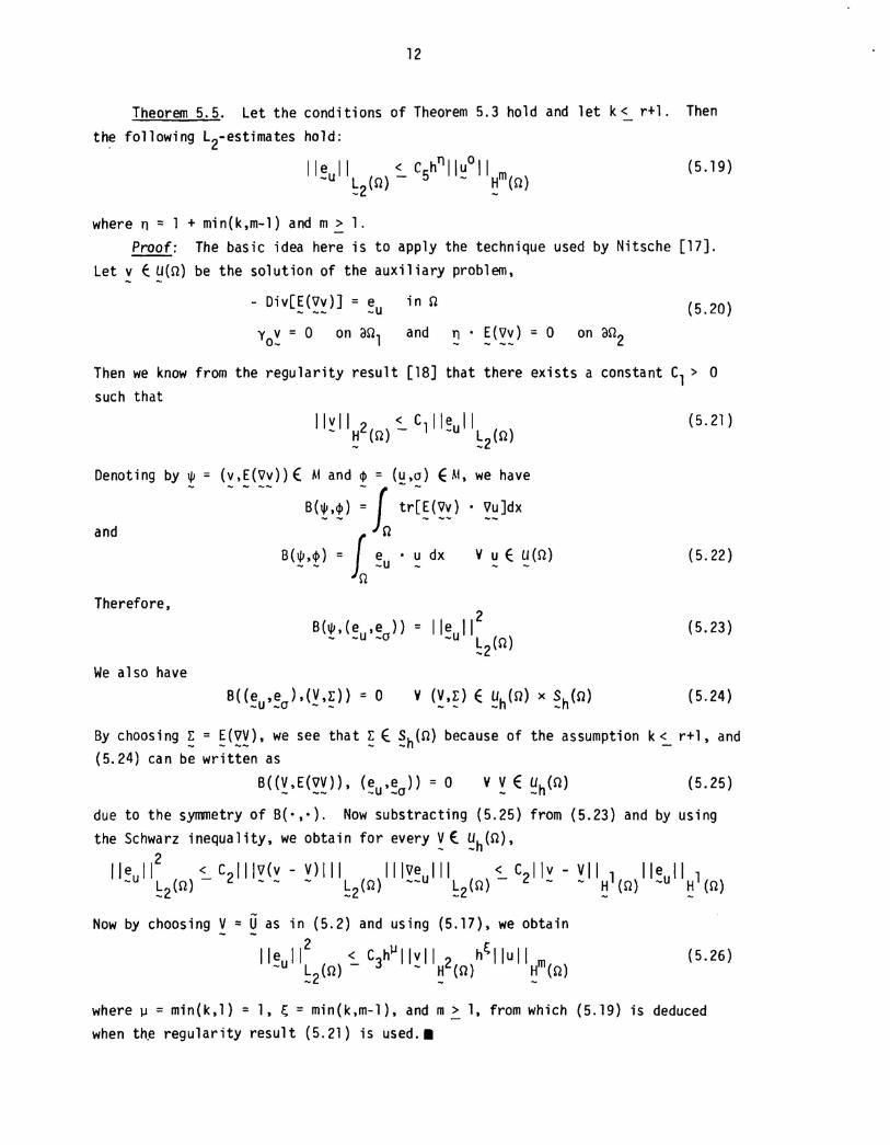
Theorem 5.5. Let the conditions of Theorem 5.3 hold and let k< r+l. Thenthe following L2-estimates hold:

(5.19)

where n : 1 + min(k,m-l) and m ~ 1.Proof: The basic idea here is to apply the technique used by Nitsche [17].

Let v c U(n) be the solution of the auxiliary problem,

- Div[E(~v)] = e in n- -- -u

Yo~ = 0 on anl and ~. ~(~~) = 0 on an2

(5.20)

Then we know from the regularity result [18] that there exists a constant Cl > 0such that

and

Denoting by IjJ = (v,E(~v)) E M and cp = (~.a) € M, we have

B(M) : l tr[~(~) • ~~]dx

B(~'2)= )[ :u • u dx VuE u(n)n

(5.21 )

(5.22)

Therefore,

We also have

B(IjI,(e ,e ))- -u-o

B((:u':o)'(~'~)) = 0

2= II:ull

l (n)-2

(5.23)

(5.24)

(5.26)

By choosing ~ = ~(~~), we see that ~ E. ~h(n) because of the assumption k< r+l, and(5.24) can be written as

B((~.E(~~)).(:u':o)) = 0 V ~ E ~h(n) (5.25)

due to the symmetry of B(·,·). Now substracting (5.25) from (5.23) and by usingthe Schwarz inequality, we obtain for every ~ ( ~h(n),

2Ileull <:"C2111~(v - V)III 111~e III <:..C211v - Vlll lie III

- L (n) - - - L (n) __u L (n) - - H (n) -u H (n)-2 -2 _2 __

Now by choosing ~ = Q as in (5.2) and using (5.17), we obtain

IIeu 112

< C3hµ IIv II 2 hE,:IIu II m- ~2(n)- - H (n) H (n)

where µ = min(k,l) = 1, E,:= min(k.m-l). and m ~ 1, from which (5.19) is deducedwhen t~e regularity result (5.21) is used .•

(6.1)

13

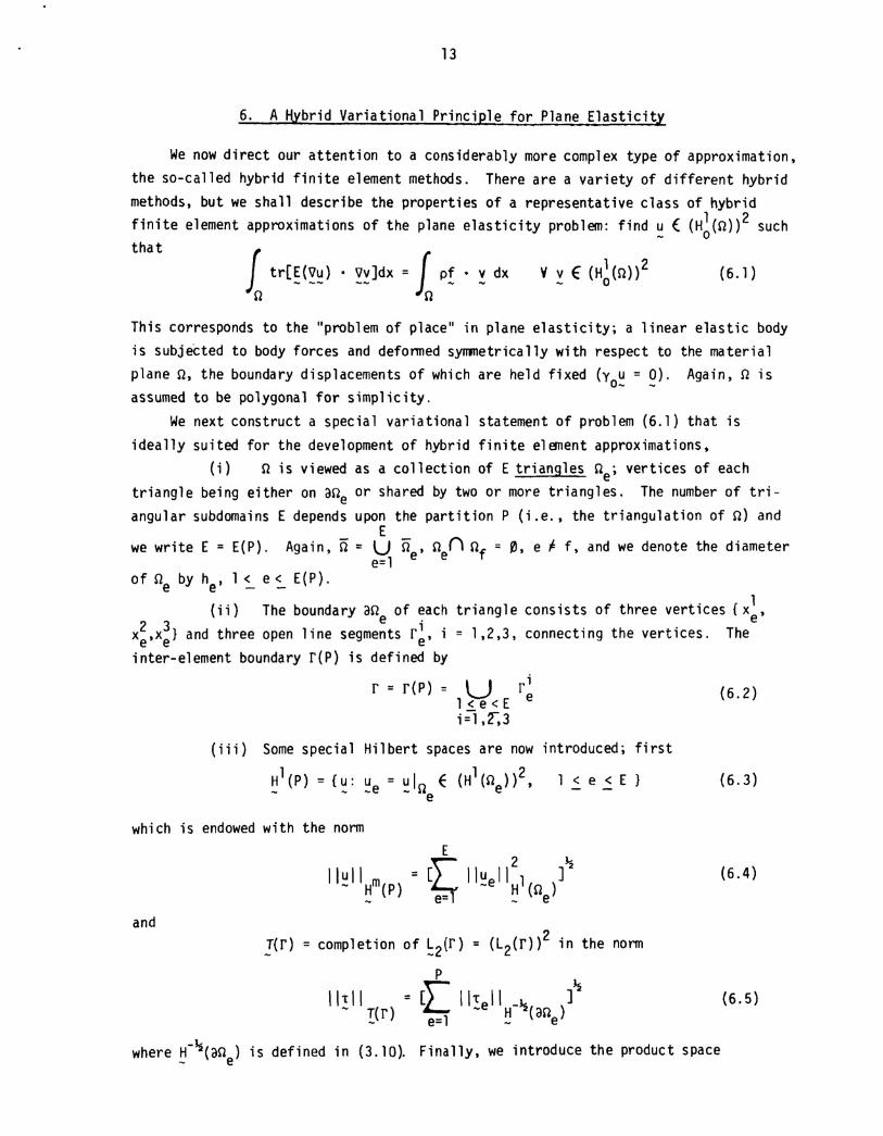
6. A HYbrid Variational Principle for Plane Elasticity

We now direct our attention to a considerably more complex type of approximation,

the so-called hybrid finite element methods. There are a variety of different hybrid

methods, but we shall describe the properties of a representative class of hybrid

finite element approximations of the plane elasticity problem: find ~ { (H~(n))2 such

that 1tr[~(~~). ~~]dx= J: p! . ~ dx Y ~ E (H~(n)2

o 0

This corresponds to the "problem of place" in plane elasticity; a linear elastic body

is subjected to body forces and deformed symmetrically with respect to the material

plane n, the boundary displacements of which are held fixed (y u = 0). Again, n is0- -

assumed to be polygonal for simplicity.

We next construct a special variational statement of problem (6.1) that is

ideally suited for the development of hybrid finite element approximations,

(i) 0 is viewed as a collection of E triangles 0 ; vertices of eachetriangle being either on ane or shared by two or more triangles. The number of tri-

angular subdomains E depends upon the partition P (i.e., the triangulation of n) andE

we write E = E(P). Again, IT= Un, 0 n Of = 9), e I: f, and we denote the diametere:l e e

of n by h , 1 < e < E(P) .e e - -(in The boundary an of each triangle consists of three vertices {xl,

2 3 e . ex ,x } and three open line segments 1", i = 1,2,3, connecting the vertices. Thee e einter-element boundary r(p) is defined by

r : r(p) = Uril<e<E ei~,~3

(iii) Some special Hilbert spaces are now introduced; first

~l(p) = {~: ~e = ~In E (Hl(ne))2, 1 < e < E }e

which is endowed with the norm

and

(6.2)

(6.3)

(6.4)

T(r) = compl etion of ~2(r) = (l2(r))2 in the norm

Lp ~IIL II = [ IIor e II _~ ]

- I(r) e=l - ~ (aoe)

where H-~(aQ ) is defined in (3.10). Finally, we introduce the product space- e

(6.5)

14

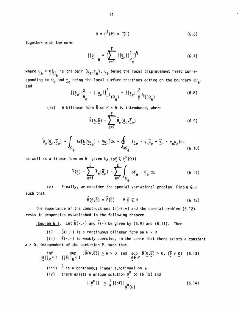
(6.6)

together with the norm

(6.7)

where ~e = ~In is the pair (~e'~e)' ~e being the local displacement field corre-e

sponding to ne and ~e being the local surface tractions acting on the boundary ane'and

(6.8)

(iv) A bilinear form B on H x H is introduced, where

B(a,e) : t Be(~e'!e)e=l

(6.9)

B (8 ,6 ) = 1 tr[E(Vu)' Vu ]dx + i (T • you + T . you )dse -e -e - --e __e -e e _e -ene ane (6.10)

(6.11)• '0 dx-e

linear form on H given by (pf f ~o(n))

F(e) = -(- F (6 ) =t f pf- L e _e -ee=l e=l ne

(v) Finally, we consider the special variational problem: Find e ~ H

as well as a

such thatA "

B( e ,6) = F (6) V !E H ( 6. 12)

The importance of the constructions (i)-(iv) and the special prOblem (6.12)rests in properties established in the following theorem.

A A

Theorem 6.1. Let B(',') and F(') be given by (6.9) and (6.11). Then

(i) B("') is a continuous bilinear form on H x H(ii) 8(',') is weakly coercive, in the sense that there exists a constant

a > 0, independent of the partition P, such that

sup /8(8,6) I > a > 0 and sup B(e,s) > 0, (6 i 0) (6.13)118/1 H~ 1 - e E H --

(iii)(i v)

A

F is a continuous linear functional on Hthere exists a unique solution ~o to (6.12) and

< ~ IIp!IIHo(n) (6.14)

1V ~ E. ~ (ne)

(6.16)

15

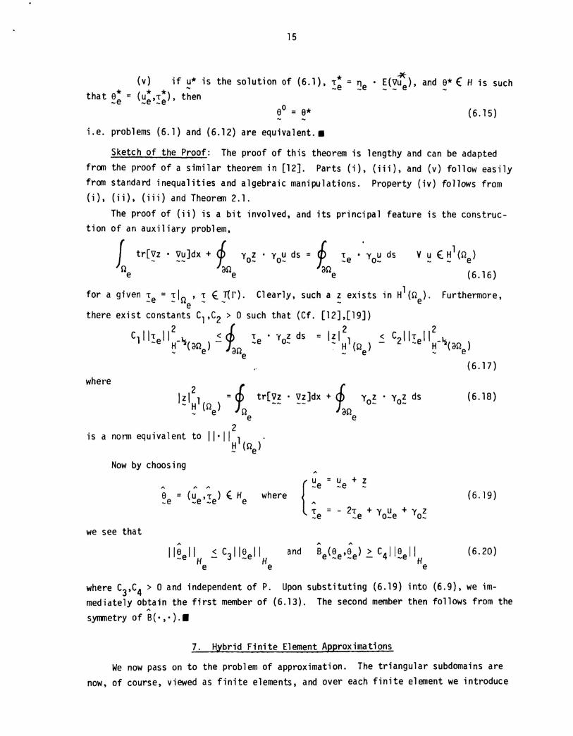
*(v) if ~* is the solution of (6.1), ~: = ~e • ~(~ue)' and a* € H is such* (* *)that ~e: ~e'~e • then

(6.15)

i.e. problems (6.1) and (6.12) are equivalent .•

Sketch of the Proof: The proof of this theorem is lengthy and can be adaptedfrom the proof of a similar theorem in [12]. Parts (i), (iii), and (v) follow easilyfrom standard inequalities and algebraic manipulations. Property (iv) follows from(i), (ii), (iii) and Theorem 2.1.

The proof of (ii) is a bit involved, and its principal feature is the construc-tion of an auxiliary problem,

f tr[vz· Vu]dx + ~ y z . y u ds = ~ Te .'y u ds- -- ~ 0- 0- ~,- o-n an ane e e

for a given ~e = ~In ' ~ E,!{r). Clearly, such a : exists in Hl(ne). Furthermore,e

there exist constants Cl,C2 > 0 such that (Cf. [12],[19])

2 1, 2 2ClllT II _l, 2. Te' Yoz ds : Izil < C211Teil _l--e H '2( an ) - - ~ H (n ) - - H '2( an )

- e an _ e - ee(6.17)

where

is a norm equivalent to

Now by choosing

= 1. tr[~~' ~~]dx + ~ yo~' yo~ dsIn 'fane e2

II . II 1 )~ (ne

(6.18)

we see that

A A

S : (u ,T ) E H_e -e -e e {

u = u + z-e -e -

where; = - 2T + Y u + Y z_e _e o-e 0_

(6.19)

A

liseII 2. C311se II and- H - He e

A A

Be(~e'~e) ~ c411~e11He

(6.20)

where C3,C4 > 0 and independent of P. Upon substituting (6.19) into (6.9), we im-mediately obtain the first member of (6.13). The second member then follows from the

A

symmetry of B(·,·) .•

7. Hybrid Finite Element Approximations

We now pass on to the problem of approximation. The triangular subdomains arenow, of course, viewed as finite elements, and over each finite element we introduce

(7.2)

(7.5)

16

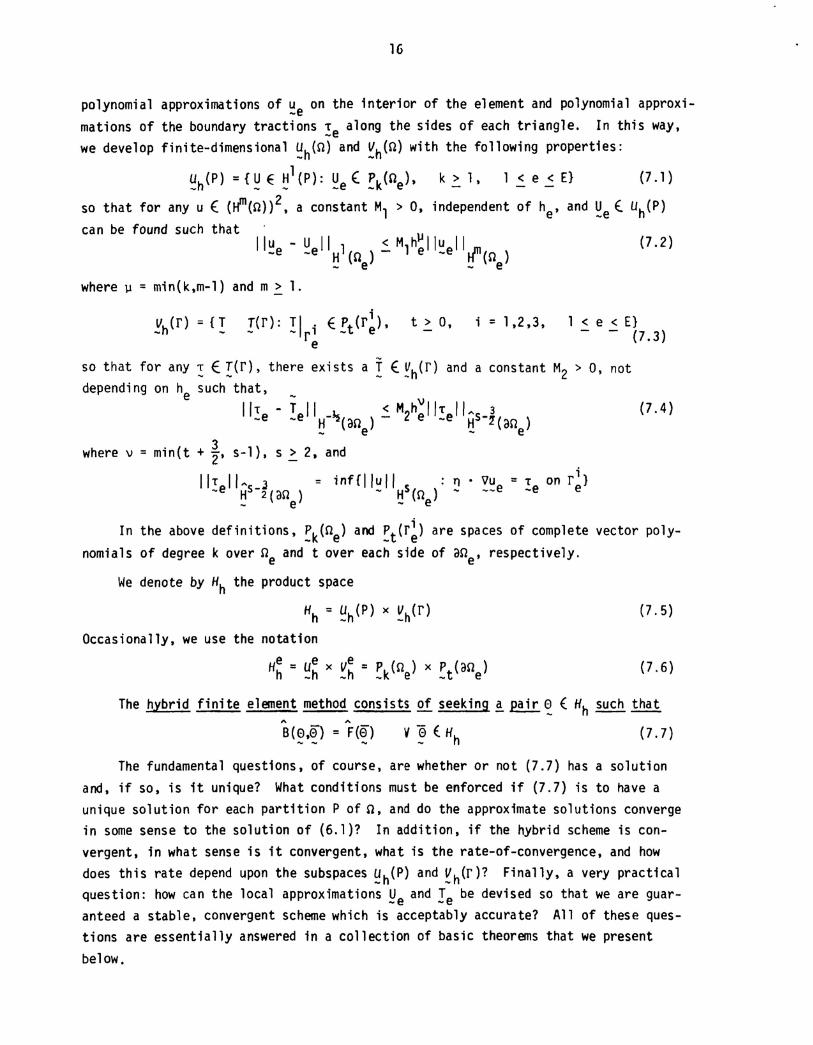
polynomial approximations of ~e on the interior of the element and polynomial approxi-mations of the boundary tractions !e along the sides of each triangle. In this way,we develop finite-dimensional ~h(n) and ~h(n) with the following properties:

~h(P):{~E~l(p):~e(~k(ne)' k>l, l<e<E} (7.1)

so that for any u E (~(n))2, a constant Ml > 0, independent of h , and U (Uh(P)e -ecan be found such that

where µ = min(k,m-l) and m > 1.

L'h(r) = { T T( r ): T liE Pt (r i ), t ~ 0, i: 1.2.3, 1 ~ e 2. E}- - - - r - e (7.3)e

so that for any ~ E !(r), there exists a !E ~h(r) and a constant M2 > 0, notdepending on he such that,

- vliT - T II 1- < M2h "T "" 3 (7.4 )-e _e H-7(an) - e -e HS-1(an)

- e - ewhere v = min(t +~, s-l), s ~ 2, and

liT II... J : inf { II u" S : 11 • Vu : T on r i}-e HS-2(an) - H (n) - __e -e e

- e - e

In the above definitions, ~k(ne) and ~t(r~) are spaces of complete vector poly-nomials of degree k over nand t over each side of an • respectively.e e

We denote by Hh the product space

Hh : ~h(P) x ~h(r)

Occasionally, we use the notation

He : ue x Ve : P (n ) x P (an )h -h _h _k e -t e (7.6)

The hybrid finite element method consists of seeking ~ pair ~ ( Hh such that,.. ,..B(e,0) : F(e) v "0 (. H (7 . 7)

- - - - hThe fundamental questions, of course, are whether or not (7.7) has a solution

and, if so, is it unique? What conditions must be enforced if (7.7) is to have aunique solution for each partition P of n, and do the approximate solutions convergein some sense to the solution of (6.l)? In addition, if the hybrid scheme is con-vergent, in what sense is it convergent. what is the rate-of-convergence, and howdoes this rate depend upon the subspaces ~h(P) and ~h(r)? Finally, a very practicalquestion: how can the local approximations Ye and Ie be devised so that we are guar-anteed a stable, convergent scheme which is acceptably accurate? All of these ques-tions are essentially answered in a collection of basic theorems that we presentbelow.

(7.8)

involves examination of the rank

basis functions for U and Te are-e -

17

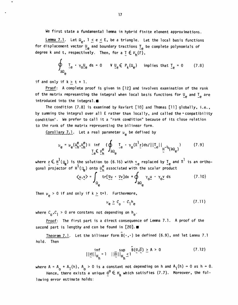
We first state a fundamental lemma in hybrid finite element approximations.

Lemma 7.1. Let net 12 e 2 E, be a triangle. Let the local basis functions

for displacement vector ~e and boundary tractions Ie be complete polynomials of

degree k and t, respectively. Then, for a !E vh(r),

~ T . y U ds: 0~ -e o-eane

if and only if k ~ t + 1.

Proof: A complete proof is given in [12] and

of the matrix representing the integral when local

introduced into the integral .•

The condition (7.8) is examined by Raviart [10] and Thomas [11] globally, i.e .•

by summing the integral over all E rather than locally, and called the "compatibilitycondition". We prefer to call it a "rank condition" because of its close rel ation

to the rank of the matrix representing the bilinear form.

Corollary 7.1. let a real parameter µ be defined bye

µ : µ (Ueh,Veh)= inf {~ T • y (nlz)ds/IIT IlL} (7.9)

e e - - e 1: -e 0 - _e H-~(an)!e~ ~h ane - e

where : ~ ~l(~) is the solution to (6.16) with ~e replaced by !e and nl is an ortho-

gonal projector of Hl(~) onto ~~ associated with the scalar product

~,~) = f tr[?~' ~~]dx + J yo~' Yo~ ds (7.10)n :rane e

Then µ > 0 if and only if k > t+l. Furthermore,e

where C .Cl > 0 are constans not depending on h .o eProof: The first part is a direct consequence of lemma 7.1. A proof of the

second part is lengthy and can be found in [20] .•A

Theorem 7.1. Let the bilinear form B("') be defined (6.9), and let lemma 7.1

hold. Then

inf11011 =1

- Hh

A

_ sup B(0.0) > A > 011011 < 1 --_ H -

h

(7.12)

where A = Ao + Al(h). Ao > 0 is a constant not depending on hand Al(h) ~ 0 as h + O.

Hence, there exists a unique ~o E Hh which satisfies (7.7). Moreover, the fol-

lowing error estimate holds:

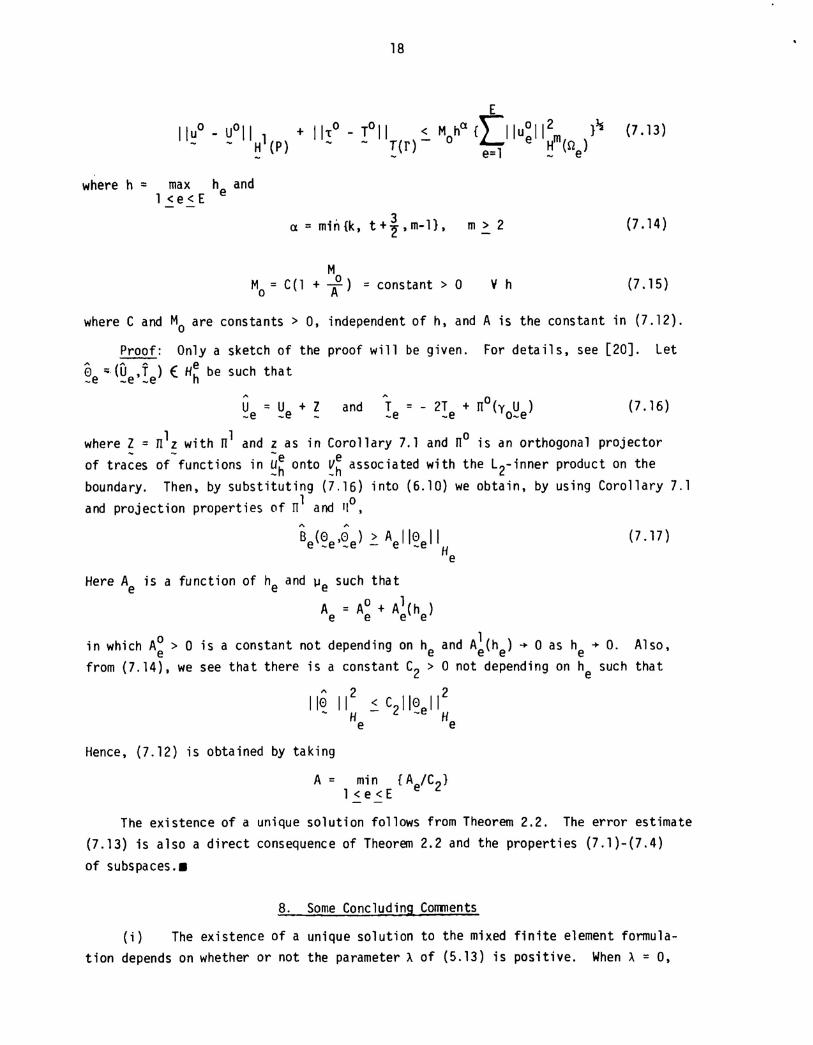
18

where h = max handl<e<E e

.' 3 }a = ml n {k, t + '2' m-l, m > 2

MMo = C (1 + AO

) = cons tant > 0 V h

(7.13 )

(7.14 )

(7.15)

where C and Mo are constants> 0, independent of h, and A is the constant in (7.12).

Proof: Only a sketch of the proof will be given. For details, see [20]. Let

~ ~(D ,f ) { Heh be such that_e -e_e

'"U = U + Z-e _e - and" 0T = - 2T + rr (y u )-e -e o-e

(7.16)

where Z = rrlz with rrl and z as in Corollary 7.1 and nO is an orthogonal projector

of tra~es of-functions in ~~ onto ~~ associated with the L2-inner product on the

boundary. Then, by substituting (7.16) into (6.10) we obtain, by using Corollary 7.1

and projection properties of nl and 1(0,

" "B ( 8 ,8 ) > A 118 IIe -e -e - e -e He

(7.17)

Here Ae is a function of he and µe such that

A = AO + Al(h )e e e e

in which AO > 0 is a constant not depending on he and Ael(h ) ~ 0 as h ~ O. Also,e e efrom (7.14), we see that there is a constant C2 > 0 not depending on he such that

" 2 2II~ IIH :: C211~e IIH

e e

Hence, (7.12) is obtained by taking

A = min {A/C2}l<e<E

The existence of a unique solution follows from Theorem 2.2. The error estimate

(7.13) is also a direct consequence of Theorem 2.2 and the properties (7.1)-(7.4)

of subspaces .•

8. Some Concluding Comments

(i) The existence of a unique solution to the mixed finite element formula-

tion depends on whether or not the parameter A of (5.13) is positive. When A = 0,

19

each ~~ is orthogonal to the space ~-l(~h(n)) of approximate strains, and this meansthat

Thus, there is no strain energy produced by the stresses E in each element due to

the gradients ~~. Therefore, ~~ must then represent a rigid rotation, and the col-

lection of elements behaves as a mechanism. Similar physical interpretations apply

to the hybrid models.

(ii) Conditions for existence of solutions of the mixed formulation are fairly

easy to fulfill by reasonable choices of the approximating polynomials, and a signi-

ficant increase in the accuracy of stress approximations over the convention displace-

ment models can be obtained. For triangular elements on which ~ and ~ are complete

polynomials of degree k and r, respectively, our l2-estimates for displacements

indicate a convergence rate of 1 order higher than the Hl estimates as expected.

(iii) The hybrid models are more delicate than the mixed. However, the order-

of-accuracy is the same as that of a comparable displacement model obtained using

polynomials of the same degree. This accuracy is obtained despite the fact that the

displacements are discontinuous across interelement boundaries, interelement conti-

nuity requirements being treated as constraints in hybrid approximations.

Acknowledgement. We gratefully acknowledge the support of this work by the U.S.Air Force Office of Scientific Research under Grant No. 74-2660.

REFERENCES

1. Prager, W. and Synge, J. L., "Approximations in Elasticity Based on the Conceptof Function Space," Q. Appl. Math., Vol. 5, No.3, pp. 241-269, 1943.

2. Herrmann, L. R., "A Bending Analysis of Plates," Proc. Conf. Matrix Meth. Struct.Mech., Wright-Patterson AFB, Ohio, AFFDl-TR66-80, 1965.

3. Reissner, E., "On a Variational Theorem in Elasticity," J. Math. Phys., Vol. 29,pp. 90-95, 1950.

4. Pian, T. H. H., and Tong. P., "Basis of Finite Element ~\ethods for Solid Con-tinua," Int. J. Num. Meth. in Eng., Vol. 1, No.1, pp. 3-28, 1969.

5. aden, J. T. and Reddy, J. N., Variational Methods in Theoretical Mechanics.Springer-Verlag, Heidelberg. Berlin, ana New York. (to appear).

6. aden, J. r. and Reddy, J. N .• "On Mixed Finite Element Approximations," SIAM J.Num. Anal:, (to appear).

7. Reddy, J. N. and aden, J. T.,"Mathematical Theory of Mixed Finite Element Ap-proximations," Q. Appl. Math. (to appear).

20

8. Ciarlet, P. G. and Raviart, P. A., "Mixed Finite Element Method for the Bihar-monic Equation," Mathematical Aspects of Finite Elements in Partial DifferentialEquations, Ed. by C. deBoor, Academic Press, N. Y., pp. 125-145,1947.

9. Johnson, C., "On the Convergence of a Mixed Finite-Element Method for PlateBending Problems," Num. Math., Vol. 21, pp. 43-62, 1973.

10. Raviart, P. A., "Hybrid Finite Element Methods for Solving 2nd Order EllipticEquations," Report , Universite Paris VI et Centre National de la RechercheScientifique, 1974.

11. Thomas, J. M., "Methodes des Elements Finis Hybrides Duaux Pour les ProblemsElliptiques du Second-Order," Report 189, Universite Paris VI et Centre Nationalde la Recherche Scientifique, 1975.

12. Babuska, 1., aden, J. T., and Lee, J. K., "Mixed-Hybrid Finite-Element Approxi-mations of Second-Order Elliptic Boundary Value Problems," (to appear).

13. Babuska, I., "Error Bounds for Finite Element Method." Num. Math., Vol. 16, pp.322-333,1971.

16. Hlavacek,!. and Necas, J., "On Inequalities of Korn's Type," Arch. Rat. Mech.Anal., Vol. 36, pp. 305-334, 1970.

17. Nitsche, J., "Ein Kriterium fur die Quasi -Optima 1itat des Ritzchen Verfahrens,"Num. Math., Vol. 11, pp. 346-348, 1968.

18. Kondratev, V. A., "Boundary Problems for Elliptic Equations with Conical orAngular Points," Trans. Moscow Math. Soc. 1967, pp. 227-313.

19. Babuska, 1., "The Finite Element Method with lagrange Multipliers," Num. Math.,Vol. 20, pp. 172-192, 1973.

"20. Lee, J. K., "A-Priori Error Estimates of Mixed and Hybrid Finite Element Methods,Ph.D. Dissertation, Div. of Engr. Mech., Univ. of Texas at Austin (forthcoming).