Theory of Consumer Behaviour Prof. Ravikesh Srivastava Lecture-7.

Theory of Consumer Behaviour

Prof. Ravikesh Srivastava

Lecture-7

Consumer Theory

Consumer theory help to have a more

complete grasp of demand theory. This ultimately leads to decisions, which improve the profitability of the manager's firm.

Effective managers will use the theory of consumer behavior to both direct employee's behavior and to choose proper pricing and other strategies.

Representing Preferences with Indifference Curves

An indifference curve is a curve that shows consumption of any combination of X and Y that give the consumer the same level of satisfaction.

The Consumer’s Preferences

Quantityof Pizza

Quantityof Pepsi

0

Indifferencecurve, I1

I2

C

B

A

D

Consumer Preference Ordering

Completeness The consumer is capable of expressing a

preference for all bundles of goods. More is Better Diminishing Marginal Rate of Substitution Transitivity

Given 3 bundles of goods: A, B & C. If A> B and B> C, then A> C. If A B and B C, then A C.

Representing Preferences with Indifference Curves

The Consumer’s Preferences The consumer is indifferent, or equally happy,

with the combinations shown at points A, B, and C because they are all on the same curve.

The Marginal Rate of Substitution The slope at any point on an indifference

curve is the marginal rate of substitution. It is the rate at which a consumer is willing to trade

one good for another. It is the amount of one good that a consumer

requires as compensation to give up one unit of the other good.

The Consumer’s Preferences

Quantityof Pizza

Quantityof Pepsi

0

Indifferencecurve, I1

I21

MRS

C

B

A

D

Four Properties of Indifference Curves

Higher indifference curves are preferred to lower ones.

Indifference curves are downward sloping.

Indifference curves do not cross. Indifference curves are bowed

inward.


Property 1: Higher indifference curves are preferred to lower ones. Consumers usually prefer more of

something to less of it. Higher indifference curves represent

larger quantities of goods than do lower indifference curves.


Property 2: Indifference curves are downward sloping. A consumer is willing to give up one good

only if he or she gets more of the other good in order to remain equally happy.

If the quantity of one good is reduced, the quantity of the other good must increase.

For this reason, most indifference curves slope downward.


Property 3: Indifference curves do not cross. Points A and B should make the consumer

equally happy. Points B and C should make the consumer

equally happy. This implies that A and C would make the

consumer equally happy. But C has more of both goods compared to

A.

Impossibility of Intersecting Indifference Curves

Quantityof Pizza

Quantityof Pepsi

0

C

A

B


Property 4: Indifference curves are bowed inward. People are more willing to trade away

goods that they have in abundance and less willing to trade away goods of which they have little.

These differences in a consumer’s marginal substitution rates cause his or her indifference curve to bow inward.

Bowed Indifference Curves

Quantityof Pizza

Quantityof Pepsi

0

Indifferencecurve

8

3

A

3

7

B

1

MRS = 6

1MRS = 14

6

14

2

Two Extreme Examples of Indifference Curves

Perfect substitutes Perfect complements


Perfect Substitutes Two goods with straight-line

indifference curves are perfect substitutes.

The marginal rate of substitution is a fixed number.

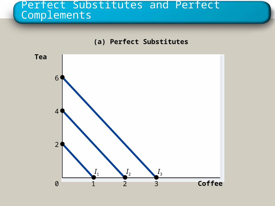
Perfect Substitutes and Perfect Complements

Coffee0

Tea

(a) Perfect Substitutes

I1 I2 I3

3

6

2

4

1

2


Perfect Complements Two goods with right-angle

indifference curves are perfect complements.

Perfect Substitutes and Perfect Complements

Right Shoes0

LeftShoes

(b) Perfect Complements

I1

I2

7

7

5

5

THE BUDGET CONSTRAINT: WHAT THE CONSUMER CAN AFFORD

The budget constraint shows the various combinations of goods the consumer can afford given his or her income and the prices of the two goods. For example, if the consumer buys no

pizzas, he can afford 500 of Pepsi (point B). If he buys no Pepsi, he can afford 100 pizzas (point A).

Alternately, the consumer can buy 50 pizzas and 250 of Pepsi.

The Consumer’s Budget Constraint

Quantityof Pizza

Quantityof Pepsi

0

Consumer’sbudget constraint

500B

100

A

The Consumer’s Budget Constraint

Quantityof Pizza

Quantityof Pepsi

0

Consumer’sbudget constraint

500B

250

50

C

100

A

THE BUDGET CONSTRAINT: WHAT THE CONSUMER CAN AFFORD

The slope of the budget constraint line equals the relative price of the two goods, that is, the price of one good compared to the price of the other.

It measures the rate at which the consumer can trade one good for the other.

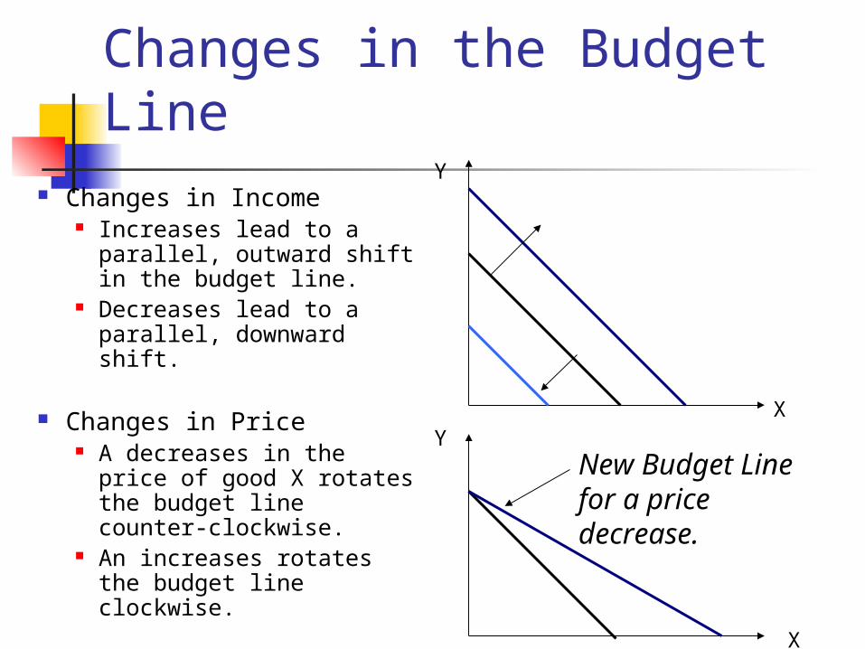
Changes in the Budget Line

Changes in Income Increases lead to a

parallel, outward shift in the budget line.

Decreases lead to a parallel, downward shift.

Changes in Price A decreases in the price

of good X rotates the budget line counter-clockwise.

An increases rotates the budget line clockwise.

X

Y

X

YNew Budget Line for a price decrease.

The Consumer’s Optimal Choices

Combining the indifference curve and the budget constraint determines the consumer’s optimal choice.

Consumer optimum occurs at the point where the highest indifference curve and the budget constraint are tangent.

The Consumer’s Optimum

Quantityof Pizza

Quantityof Pepsi

0

Budget constraint

I1I2

I3

Optimum

AB

How Changes in Income Affect the Consumer’s Choices

An increase in income shifts the budget constraint outward. The consumer is able to choose a

better combination of goods on a higher indifference curve.

An Increase in Income

Quantityof Pizza

Quantityof Pepsi

0

New budget constraint

I1

I2

2. . . . raising pizza consumption . . .

3. . . . andPepsiconsumption.

Initialbudgetconstraint

1. An increase in income shifts thebudget constraint outward . . .

Initialoptimum

New optimum

How Changes in Income Affect the Consumer’s Choices

Normal versus Inferior Goods If a consumer buys more of a good

when his or her income rises, the good is called a normal good.

If a consumer buys less of a good when his or her income rises, the good is called an inferior good.

An Inferior Good

Quantityof Pizza

Quantityof Pepsi

0



I1 I2

1. When an increase in income shifts thebudget constraint outward . . .3. . . . but

Pepsiconsumptionfalls, makingPepsi aninferior good.

2. . . . pizza consumption rises, making pizza a normal good . . .

Initialoptimum

New optimum

How Changes in Prices Affect Consumer’s Choices

A fall in the price of any good rotates the budget constraint outward and changes the slope of the budget constraint.

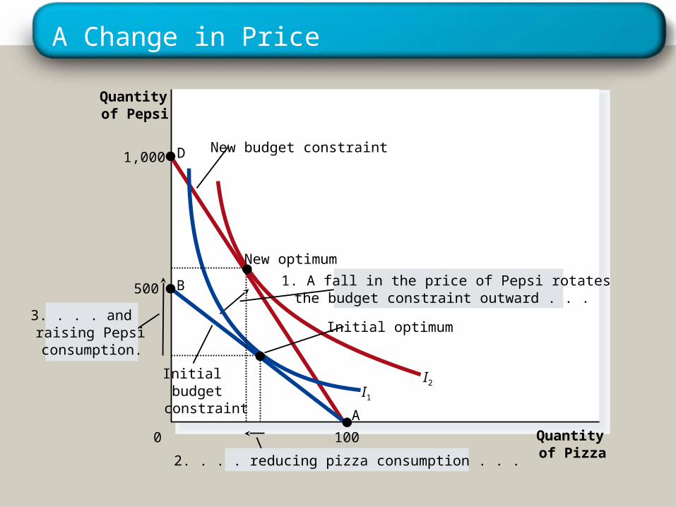
A Change in Price

Quantityof Pizza

Quantityof Pepsi

0

1,000 D

500 B

100

A

I1I2

Initial optimum



1. A fall in the price of Pepsi rotates the budget constraint outward . . .

3. . . . andraising Pepsiconsumption.

2. . . . reducing pizza consumption . . .

New optimum

Income and Substitution Effects

A price change has two effects on consumption. An income effect A substitution effect


The Income Effect The income effect is the change in

consumption that results when a price change moves the consumer to a higher or lower indifference curve.

The Substitution Effect The substitution effect is the change in

consumption that results when a price change moves the consumer along an indifference curve to a point with a different marginal rate of substitution.


Quantityof Pizza

Quantityof Pepsi

0

I1

I2A

Initial optimum



Substitutioneffect

Substitution effect

Incomeeffect

Income effect

B

C New optimum

Theory of Consumer Behaviour Prof. Ravikesh Srivastava Lecture-7.

Documents

Transcript of Theory of Consumer Behaviour Prof. Ravikesh Srivastava Lecture-7.