Theory Comparison between Propane and Methane...
6
International Journal of Current Engineering and Technology E-ISSN 2277 – 4106, P-ISSN 2347 – 5161 ©2015 INPRESSCO ® , All Rights Reserved Available at http://inpressco.com/category/ijcet Research Article 2429| International Journal of Current Engineering and Technology, Vol.5, No.4 (Aug 2015) Theory Comparison between Propane and Methane Combustion inside the Furnace Dhafer A. Hamzah †* † Al-Qadisiyah University, College of Engineering, Iraq Accepted 01 July 2015, Available online 11 July 2015, Vol.5, No.4 (Aug 2015) Abstract This study used ANSYS FLUENT to model the transport, mixing, and reaction of chemical species. The reaction system was defined by using and modifying a mixture-material entry in the ANSYS FLUENT database. The study used propane C3H8 for simulation of hydrocarbon combustion and comparison the results with another study for methane CH4combustion for find the difference in combustion temperature and effect of change in specific heat as a function of temperature. The study found that the maximum temperature for propane is less than methane for both states in constant and change of specific heat, and the reason for this attribute because of methane has octane number higher than propane and this effects on flame propagation speed and flame temperature also we note the distribution of maximum temperature is mostly near to wall and axis region as shown in the results . This distribution helps to know where will be the maximum temperature for varies applications. Also the NOx production in this study was dominated by the thermal NO mechanism. This mechanism is very sensitive to temperature. Every effort should be made to ensure that the temperature solution is not over predicted, since this will lead to unrealistically high predicted levels of NO. Because of all this the emission of NOx for methane is more than propane as result for high temperature for methane combustion Keywords: Propane, Methane Combustion etc. Background 1 Propane has been tested in fleet vehicles for a number of years. It's a good high octane number for SI engine fuel and produces less emission than gasoline about 60% less co, 30%less HC, and 20%less NOx (Pulkrabek).Propane stored as a liquid under pressure and delivered through a high pressure line to the engine. In this study, you will use the generalized eddy-dissipation model to analyze the methane-air combustion system. The combustion will be modeled using a global one step reaction mechanism, assuming complete conversion of the fuel to CO2 and H2O. The reaction equation is C3H8 + 5O2 →3CO2 + 4H2O (1) This reaction will be defined in terms of stoichiometric coefficients, formation enthalpies, and parameters that control the reaction rate. The reaction rate will be determined assuming that turbulent mixing is the rate- limiting process, with the turbulence-chemistry interaction modeled using the eddy-dissipation model. *Corresponding author: Dhafer A. Hamzah Problem Description The cylindrical combustor considered in this study (Ansys inc.) is shown in Figure 1. Figure 1 Problem description The flame considered is a turbulent diffusion flame. A small nozzle in the center of the combustor introduces propane (C3H8) at 80 m/s. Ambient air enters the combustor coaxially at 0.5 m/s. The overall equivalence ratio is approximately 0.76 (approximately 28% excess air). The high-speed methane jet initially expands with little interference from the outer wall, and entrains and mixes with the low-speed air. The Reynolds number based on the methane jet diameter is approximately 5.7 × 10 3 .
-
Upload
truongdung -
Category
Documents
-
view
243 -
download
1
Transcript of Theory Comparison between Propane and Methane...

International Journal of Current Engineering and Technology E-ISSN 2277 – 4106, P-ISSN 2347 – 5161 ©2015 INPRESSCO®, All Rights Reserved Available at http://inpressco.com/category/ijcet
Research Article
2429| International Journal of Current Engineering and Technology, Vol.5, No.4 (Aug 2015)
Theory Comparison between Propane and Methane Combustion inside the Furnace Dhafer A. Hamzah†* †Al-Qadisiyah University, College of Engineering, Iraq
Accepted 01 July 2015, Available online 11 July 2015, Vol.5, No.4 (Aug 2015)
Abstract This study used ANSYS FLUENT to model the transport, mixing, and reaction of chemical species. The reaction system was defined by using and modifying a mixture-material entry in the ANSYS FLUENT database. The study used propane C3H8 for simulation of hydrocarbon combustion and comparison the results with another study for methane CH4combustion for find the difference in combustion temperature and effect of change in specific heat as a function of temperature. The study found that the maximum temperature for propane is less than methane for both states in constant and change of specific heat, and the reason for this attribute because of methane has octane number higher than propane and this effects on flame propagation speed and flame temperature also we note the distribution of maximum temperature is mostly near to wall and axis region as shown in the results . This distribution helps to know where will be the maximum temperature for varies applications. Also the NOx production in this study was dominated by the thermal NO mechanism. This mechanism is very sensitive to temperature. Every effort should be made to ensure that the temperature solution is not over predicted, since this will lead to unrealistically high predicted levels of NO. Because of all this the emission of NOx for methane is more than propane as result for high temperature for methane combustion Keywords: Propane, Methane Combustion etc. Background
1Propane has been tested in fleet vehicles for a number
of years. It's a good high octane number for SI engine
fuel and produces less emission than gasoline about
60% less co, 30%less HC, and 20%less NOx
(Pulkrabek).Propane stored as a liquid under
pressure and delivered through a high pressure line to
the engine. In this study, you will use the generalized
eddy-dissipation model to analyze the methane-air
combustion system. The combustion will be modeled
using a global one step reaction mechanism, assuming
complete conversion of the fuel to CO2 and H2O. The
reaction equation is
C3H8 + 5O2 →3CO2 + 4H2O (1)
This reaction will be defined in terms of stoichiometric
coefficients, formation enthalpies, and parameters that
control the reaction rate. The reaction rate will be
determined assuming that turbulent mixing is the rate-
limiting process, with the turbulence-chemistry
interaction modeled using the eddy-dissipation model. *Corresponding author: Dhafer A. Hamzah
Problem Description The cylindrical combustor considered in this study (Ansys inc.) is shown in Figure 1.
Figure 1 Problem description
The flame considered is a turbulent diffusion flame. A
small nozzle in the center of the combustor introduces
propane (C3H8) at 80 m/s. Ambient air enters the
combustor coaxially at 0.5 m/s. The overall
equivalence ratio is approximately 0.76
(approximately 28% excess air). The high-speed
methane jet initially expands with little interference
from the outer wall, and entrains and mixes with the
low-speed air. The Reynolds number based on the
methane jet diameter is approximately 5.7 × 10³.

Dhafer A. Hamzah Theory Comparison between Propane and Methane Combustion inside the Furnace
2430| International Journal of Current Engineering and Technology, Vol.5, No.4 (Aug 2015)
Creating the cylindrical combustor and mesh generation The shape of cylindrical combustor is formed by solid
program and exports it to workbench of Ansys 12 the
shape will be plane for two dimension and the
dimension be in SI units (m). Then the ansys program
will mesh the shape and It is a good practice to check
the mesh after you manipulate it (i.e., scale, convert to
polyhedra, merge, separate, fuse, add zones, or smooth
and swap.)This will ensure that the quality of the mesh
has not been compromised Figure 2.
Figure 2 Mesh generation Model Species Transport and Finite-Rate Chemistry ANSYS FLUENT can model the mixing and transport of chemical species by solving conservation equations describing convection, diffusion, and reaction sources for each component species. Multiple simultaneous chemical reactions can be modeled, with reactions occurring in the bulk phase (volumetric reactions) and/or on wall or particle surfaces, and in the porous region. Species transport modeling capabilities, both with and without reactions. Note that you may also want to consider modeling your turbulent reacting flame using the mixture fraction approach (for non-premixed systems) or the reaction progress variable approach (for premixed systems, the partially premixed approach, or the composition PDF Transport approach. The study will use to solve conservation equations for chemical species, ANSYS FLUENT predicts the local mass fraction of each species, Yi, through the solution of a convection, diffusion equation for the ith species. This conservation equation takes the following general form:
( ) ( ) (2)
Mass Diffusion in Turbulent Flows In turbulent flows, ANSYS FLUENT computes the mass diffusion in the following form:
(
)
(3)
The default Sct is 0.7. Note that turbulent diffusion generally overwhelms laminar diffusion, and the specification of detailed laminar diffusion properties in turbulent flows is generally not necessary.
Treatment of Species Transport in the Energy Equation For many multi component mixing flows, the transport of enthalpy due to species diffusion Magnussen ∑
(4) can have a significant effect on the enthalpy field and should not be neglected. In particular, when the Lewis number
(5)
for any species is far from unity, neglecting this term can lead to significant errors. ANSYSFLUENT will include this term by default. The Eddy-Dissipation Model Most fuels are fast burning, and the overall rate of reaction is controlled by turbulent mixing. In non-premixed flames, turbulence slowly convects /mixes fuel and oxidizer into the reaction zones where they burn quickly. In premixed flames, the turbulence slowly convects/mixes cold reactants and hot products into the reaction zones, where reaction occurs rapidly. In such cases, the combustion is said to be mixing-limited, and the complex, and often unknown, chemical kinetic rates can be safely neglected, ANSYS FLUENT provides a turbulence-chemistry interaction model, based on the work of (Magnussen and Hjertager), called the eddy-dissipation model. The net rate of production of species i due to reaction r, Ri,r, is given by the smaller (i.e., limiting value) of the two expressions below:
(
) (6)
∑
∑
(7)
Reaction rates are assumed to be controlled by the turbulence, so expensive Arrhenius chemical kinetic calculations can be avoided. The model is computationally cheap, but, for realistic results, only one or two step heat-release mechanisms should be used.
Results and discussions The study will discuss mainly the static temperature in case of constant specific heat and variation of specific heat as function to temperature and distribution of temperature and outlet temperature and comparisons it with static temperature for methane combustion for validation to another study. Also the emission for NOx and the difference between methane as fuel and propane in our study.

Dhafer A. Hamzah Theory Comparison between Propane and Methane Combustion inside the Furnace
2431| International Journal of Current Engineering and Technology, Vol.5, No.4 (Aug 2015)
Iteration and residuals The initial calculation will be performed assuming that all properties except density are constant. The use of constant transport properties (viscosity, thermal conductivity, and mass diffusivity coefficients) is acceptable because the flow is fully turbulent. The molecular transport properties will play a minor role compared to turbulent transport. The assumption of constant specific heat, however, has a strong effect on the combustion solution. Figure (3) shows the solution will converge in approximately 250 iterations. Then the study will change the specific heat property definition in step with varying heat capacity as a function of temperature (polynomial equation) and the solution will be converge in approximately 375 iterations Figure (4). The residuals will jump significantly as the solution adjusts to the new specific heat representation. The solution will converge after approximately 125 additional iterations.
Figure 3 Converge history for constant Cp
Figure 4 Converge history for variable Cp
Temperature of reaction In Figure (5) we observe the static temperature for combustion of propane at constant heat capacity is 2900 K and is less than for methane combustion for another study (Ansys inc) which is above of 3000 K the reason is attribute to octane number for methane is higher than propane and this effect on flame
propagation speed which will be more in methane so that increase the reaction speed and temperature of the reaction. Also the molecular weight for propane is more than methane which effect on the generation of water molecular, also the heating value for methane is higher than propane this is a more reason for this differences. The peak temperature, predicted using a constant heat capacity of 1000 J/kg − K, is over 2900 K. This over prediction of the flame temperature can be remedied by a more realistic model for the temperature and composition dependence of the heat capacity, as illustrated in the Figure (6). The peak temperature has dropped to
approximately 2160K as a result of the temperature
and composition-dependent specific heat (Ruud
Beerkens & Adriaan Lankhorst). The strong
temperature and composition dependence of the
specific heat has a significant impact on the predicted
flame temperature. The mixture specific heat is largest
where the C3H8 is concentrated, near the fuel inlet, and
where the temperature and combustion product
concentrations are large. The increase in heat capacity,
relative to the constant value used before, substantially
lowers the peak flame temperature Figure (7).
Present study (Propane combustion)
Comparison study (methane combustion)
Figure 5 Contours of static temperature- constant Cp
Dhafer A. Hamzah Theory Comparison between Propane and Methane Combustion inside the Furnace
2432| International Journal of Current Engineering and Technology, Vol.5, No.4 (Aug 2015)
Present study (Propane combustion)
Comparison study (methane combustion)
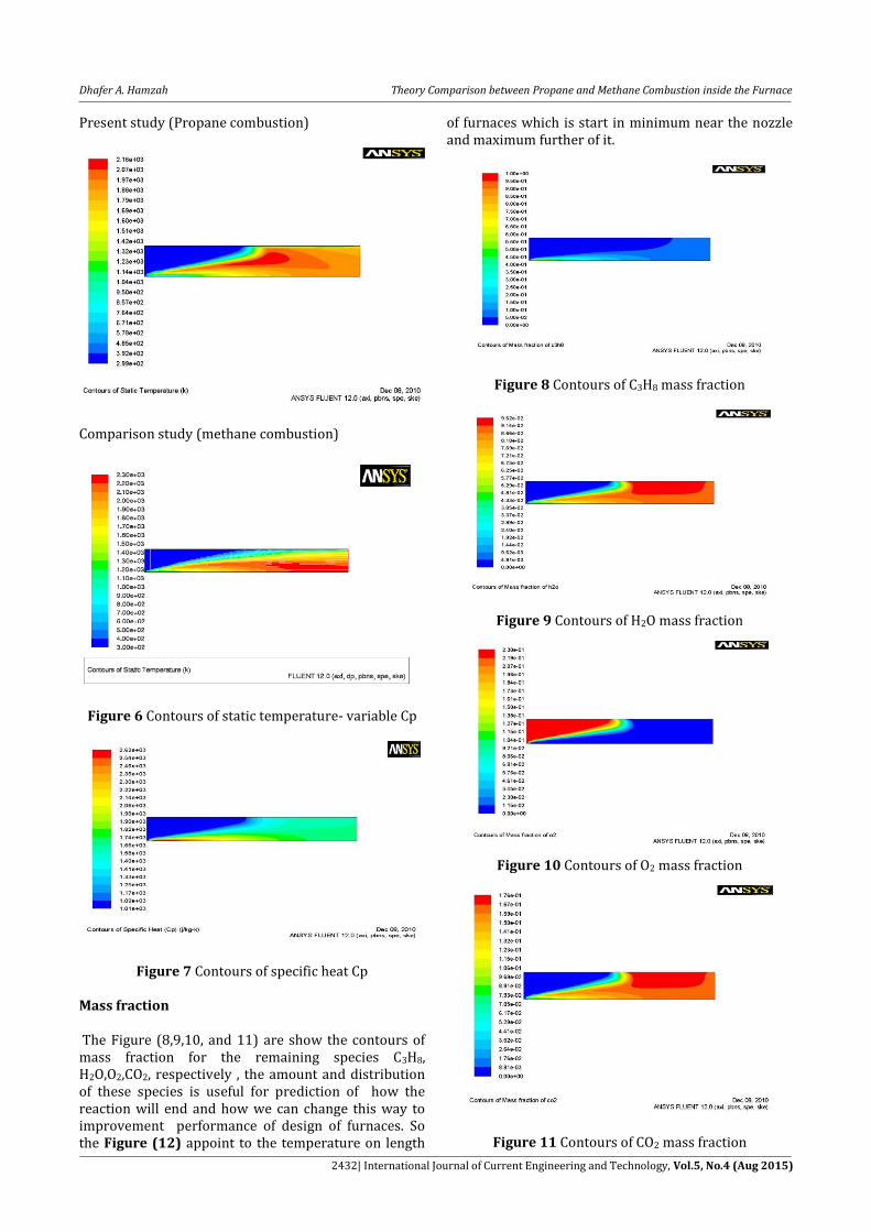
Figure 6 Contours of static temperature- variable Cp
Figure 7 Contours of specific heat Cp
Mass fraction The Figure (8,9,10, and 11) are show the contours of mass fraction for the remaining species C3H8, H2O,O2,CO2, respectively , the amount and distribution of these species is useful for prediction of how the reaction will end and how we can change this way to improvement performance of design of furnaces. So the Figure (12) appoint to the temperature on length
of furnaces which is start in minimum near the nozzle and maximum further of it.
Figure 8 Contours of C3H8 mass fraction
Figure 9 Contours of H2O mass fraction
Figure 10 Contours of O2 mass fraction
Figure 11 Contours of CO2 mass fraction

Dhafer A. Hamzah Theory Comparison between Propane and Methane Combustion inside the Furnace
2433| International Journal of Current Engineering and Technology, Vol.5, No.4 (Aug 2015)
Figure 12 The relation between axis static temperature and the length of furnace
NOx Prediction In this section you will extend the ANSYS FLUENT model to include the prediction of NOx.
Figure 13 Contours of NO mass fraction –Prompt and
Thermal NOx formation
Figure 14 Converge history for NOx model
The study will calculate the formation of both thermal and prompt NOx, the peak concentration of NO is located in a region of high temperature where oxygen and nitrogen are available (Ronald A. Jordan) and less than in methane combustion because of lowering of
flame temperature and distribution of mass fraction for species. Figure (13). The prediction of NOx formation in a postprocessing mode, with the flow field, temperature, and hydrocarbon combustion species concentrations fixed. Hence, only the NO equation will be computed. Prediction of NO in this mode is justified on the grounds that the NO concentrations are very low and have negligible impact on the hydrocarbon combustion prediction. The solution will converge in approximately 7 iterations Figure (14). Combustion kinetics
Due to the high local Reynolds Numbers occurring in
combustion in furnaces, the flow, in general, is highly
turbulent Figure (15), meaning that eddies of different
sizes lead to random fluctuations (in time & space) of
flow velocity Figure (16), temperature and species
concentrations. A typical important aspect of turbulent
flows is the increased level of mixing of momentum,
heat and mass, as compared to laminar flows. In
turbulence modeling this usually is described by the
eddy viscosity concept and a typical model frequently
used in engineering is the two-equation k-turbulence
model (Launder & Spalding).
Figure 15a Contours for turbulent intensity
Figure 15b Plot for turbulent intensity of axis’

Dhafer A. Hamzah Theory Comparison between Propane and Methane Combustion inside the Furnace
2434| International Journal of Current Engineering and Technology, Vol.5, No.4 (Aug 2015)
Figure 16 Plot for axial velocity of axis
Table 1 Summarizing results
Peak temperature K
Outlet temperature
(K)
Outlet velocity (m/s)
Outlet mass fraction of
Pollutant NO
2900 (constant Cp)
2160 (variable Cp)
2637.7017 1878.1829
4.95788 3.5646446
0.00049750332
Conclusion 1. There is possibility for using propane as fuel for
furnaces and reduce the emission of NOx with gotten the desired temperature.
2. The use of a constant Cp results in a significant over prediction of the peak temperature. The average exit velocity and temperature are also over predicted
3. The variable Cp solution produces dramatic improvements in the predicted results.
References
ANSYS, Inc. (March 12, 2009), Modeling Species Transport
and Gaseous Combustion Ronald A. Jordan (2001), Furnace combustion sensor test
results, September
Launder B.E., Spalding D.B. (1972), Mathematical Modeling of Turbulence, Academic Press, London2
Ruud Beerkens & Adriaan Lankhorst (2009), Combustion& fuels for class furnace Tutorial Vancouver Text on Combustion in Glass Furnaces
B. F. Magnussen and B. H. Hjertager (1976) On mathematical models of turbulent combustion with special emphasis on soot formation and combustion. In 16th Symp. (Int’l.) on Combustion. The Combustion Institute.
William J. Pulkrabekm (1997) fundamentals engineering in internal combustion, Hall inc.
B. F. Magnussen (1981) On the Structure of Turbulence and a Generalized Eddy Dissipation Concept for Chemical Reaction in Turbulent Flow. Nineteeth AIAA Meeting, St. Louis.
Meaning Symbols
Species i
Local mass fraction of each species Yi
Net rate of production of species i Ri
Rate of creation Si
Diffusion flux of species i Ji
Mass diffusion coefficient for
species i Di,m
Thermal diffusion coefficient DT,i
Turbulent Schmidt number Sct
Turbulent viscosity tµ
Enthalpy of species hi
Lewis number Lei
Mass fraction of any product
species YP
Mass fraction of a particular
reactant YR
Empirical constant equal to 4.0 A
Empirical constant equal to 0.5 B
Products and Reactants P and R
Turbulent mixing rate ⁄
Molecular weight of species i Mw,i
Turbulent diffusivity Dt
Stoichiometric coefficient for
reactant i in reaction r v'i,r
Stoichiometric coefficient for
product i in reaction r v''i,r