Theory and numerical analysis of Volterra functional...
96
Theory and numerical analysis of Volterra functional equations (TU Chemnitz, 22-26 September 2008) Hermann Brunner Department of Mathematics and Statistics Memorial University of Newfoundland St. John’s, NL Canada A1C 5S7 [email protected] and Department of Mathematics Hong Kong Baptist University Kowloon Tong Hong Kong SAR P.R. China [email protected] 28 July 2008 Summary The qualitative and quantitative analyses of numerical methods delay differential equations (DDEs) are now quite well understood, as reflected in the recent monograph by Bellen and Zennaro (2003). This is in remarkable contrast to the situation in the numerical analysis of more general Volterra functional equations in which delays occur in connection with memory terms described by Volterra integral operators. The complexity of the convergence and asymptotic stability analysis has its roots in a number of aspects not present in DDEs: the problems have distributed delays; kernels in the Volterra operators may be weakly singular; a second discretisation step (approximation of the memory term by feasible quadrature processes) will in general be necessary before solution approximations can be computed. These notes are intended to provide an introduction to functional integral and integro- differential equations of Volterra type and their numerical analysis, focusing on collocation methods. They contain background material (and references), and also describe the “state of the art” in the numerical analysis. In addition, they reveal that we still have a long way to go before we reach a level of insight into the numerical analysis of Volterra functional equations comparable to the one that has been achieved for delay differential equations. This is an updated and expanded version of the paper that originally appeared in Acta Numerica 13 (2004), 55-145. 1
Transcript of Theory and numerical analysis of Volterra functional...

Theory and numerical analysis ofVolterra functional equations
(TU Chemnitz, 22-26 September 2008)
Hermann Brunner
Department of Mathematics and StatisticsMemorial University of Newfoundland
St. John’s, NLCanada A1C 5S7
andDepartment of Mathematics
Hong Kong Baptist UniversityKowloon Tong
Hong Kong SARP.R. China
28 July 2008
Summary
The qualitative and quantitative analyses of numerical methods delay differential equations(DDEs) are now quite well understood, as reflected in the recent monograph by Bellen andZennaro (2003). This is in remarkable contrast to the situation in the numerical analysisof more general Volterra functional equations in which delays occur in connection withmemory terms described by Volterra integral operators. The complexity of the convergenceand asymptotic stability analysis has its roots in a number of aspects not present in DDEs:the problems have distributed delays; kernels in the Volterra operators may be weaklysingular; a second discretisation step (approximation of the memory term by feasiblequadrature processes) will in general be necessary before solution approximations can becomputed.These notes are intended to provide an introduction to functional integral and integro-differential equations of Volterra type and their numerical analysis, focusing on collocationmethods. They contain background material (and references), and also describe the “stateof the art” in the numerical analysis. In addition, they reveal that we still have a long wayto go before we reach a level of insight into the numerical analysis of Volterra functionalequations comparable to the one that has been achieved for delay differential equations.
This is an updated and expanded version of the paper that originally appearedin Acta Numerica 13 (2004), 55-145.
1

CONTENTS 2
Contents
1 Introduction 41.1 Early Volterra functional integral equations . . . . . . . . . . . . . . . . . . 4
1.1.1 Volterra integral equations with proportional delays . . . . . . . . . 41.1.2 The Volterra delay VIDEs of population dynamics . . . . . . . . . . 4
1.2 Volterra functional equations as mathematical models . . . . . . . . . . . . 5
2 Basic theory of Volterra functional equations (I) 82.1 Second-kind Volterra integral equations with non-vanishing delays . . . . . 82.2 First-kind VIEs with non-vanishing delays . . . . . . . . . . . . . . . . . . . 142.3 VFIDEs with non-vanishing delays . . . . . . . . . . . . . . . . . . . . . . . 152.4 Volterra functional equations with weakly singular kernels . . . . . . . . . . 17
3 Collocation methods for VFEs with non-vanishing delays 193.1 Numerical analysis of VFEs: an overview . . . . . . . . . . . . . . . . . . . 19
3.1.1 DDEs . . . . . . . . . . . . . . . . . . . . . . . . . . . . . . . . . . . 193.1.2 VFIEs of the second kind . . . . . . . . . . . . . . . . . . . . . . . . 203.1.3 VFIDEs . . . . . . . . . . . . . . . . . . . . . . . . . . . . . . . . . . 21
3.2 Collocation methods for VFIEs with non-vanishing delays . . . . . . . . . . 213.2.1 Collocation spaces for classical Volterra equations . . . . . . . . . . 223.2.2 Constrained and θ-invariant meshes . . . . . . . . . . . . . . . . . . 22
3.3 VFIEs of the second kind . . . . . . . . . . . . . . . . . . . . . . . . . . . . 243.3.1 The collocation equations . . . . . . . . . . . . . . . . . . . . . . . . 243.3.2 Global convergence results . . . . . . . . . . . . . . . . . . . . . . . . 283.3.3 Local superconvergence results . . . . . . . . . . . . . . . . . . . . . 313.3.4 Nonlinear VFIEs . . . . . . . . . . . . . . . . . . . . . . . . . . . . . 33
3.4 Collocation for VFIDEs with non-vanishing delays . . . . . . . . . . . . . . 353.4.1 The collocation equations . . . . . . . . . . . . . . . . . . . . . . . . 353.4.2 Global convergence results . . . . . . . . . . . . . . . . . . . . . . . . 373.4.3 Local superconvergence results . . . . . . . . . . . . . . . . . . . . . 39
4 Basic theory of Volterra functional equations (II) 414.1 The pantograph equation: ca. 1971 . . . . . . . . . . . . . . . . . . . . . . . 414.2 Second-kind VFIEs with proportional delays . . . . . . . . . . . . . . . . . . 434.3 First-kind Volterra integral equations with vanishing delays . . . . . . . . . 454.4 VFIDEs with proportional delays . . . . . . . . . . . . . . . . . . . . . . . . 464.5 Embedding techniques . . . . . . . . . . . . . . . . . . . . . . . . . . . . . . 48
5 Collocation methods for pantograph-type VFEs 515.1 Numerical analysis of pantograph-type equations: an overview . . . . . . . . 51
5.1.1 Numerical analysis of the pantograph DDE . . . . . . . . . . . . . . 515.1.2 Volterra functional equations with proportional delays . . . . . . . . 52
5.2 Vanishing delays and uniform meshes: overlap . . . . . . . . . . . . . . . . . 525.3 Second-kind VFIEs with proportional delays . . . . . . . . . . . . . . . . . . 54
5.3.1 The structure of the cllocation equations . . . . . . . . . . . . . . . . 545.3.2 Optimal orders of convergence . . . . . . . . . . . . . . . . . . . . . 59
5.4 First-kind VFIEs with proportional delays . . . . . . . . . . . . . . . . . . . 635.5 VFIDEs with proportional delays . . . . . . . . . . . . . . . . . . . . . . . . 65
5.5.1 Optimal convergence estimates . . . . . . . . . . . . . . . . . . . . . 665.6 Collocation using geometric meshes . . . . . . . . . . . . . . . . . . . . . . . 685.7 Equations with nonlinear vanishing delays . . . . . . . . . . . . . . . . . . . 70

CONTENTS 3
5.8 VFEs with multiple vanishing delays . . . . . . . . . . . . . . . . . . . . . . 70
6 Additional topics and concluding remarks 726.1 VFIEs and VFIDEs with weakly singular kernels . . . . . . . . . . . . . . . 726.2 VFIEs and VFIDEs with advanced arguments . . . . . . . . . . . . . . . . . 736.3 Integral-algebraic VFEs . . . . . . . . . . . . . . . . . . . . . . . . . . . . . 746.4 VFEs with state-dependent delays . . . . . . . . . . . . . . . . . . . . . . . 746.5 Asymptotic behaviour of collocation solutions . . . . . . . . . . . . . . . . . 74
7 References 777.1 References (≤ 2004) . . . . . . . . . . . . . . . . . . . . . . . . . . . . . . . 777.2 Additional references . . . . . . . . . . . . . . . . . . . . . . . . . . . . . . . 94

1 INTRODUCTION 4
1 Introduction
1.1 Early Volterra functional integral equations
1.1.1 Volterra integral equations with proportional delays
In his paper of 1897 (a sequel to his four fundamental papers that appeared in 1896) VitoVolterra studied the “invertibility” of the “definite integral” (using his terminology andnotation)
f(y)− f(0) =∫ y
αyθ(x)H(x, y) dx, 0 < y < a, (1.1)
where the parameter α in the delay function αy satisfies 0 < α < 1. The functionsf, f ′, H, Hy are assumed to be continuous on their respective domains. The integraloperator describing this first-kind integral equation has two variable limits of integration,and the lower limit represents a proportional delay vanishing at t = 0. Volterra precededthe analysis of the existence and uniqueness of the solution θ ∈ C[0, a] by the followingobservation (Volterra (1897, pp. 156-157). Suppose that the given (real-valued) functionsλ and ϕ are continuous on [0, a], with |λ(0)| ≤ 1, and consider the infinite series
θ(x) := ϕ(x) +∞∑
j=1
αj
j−1∏l=0
λ(αlx)
ϕ(αjx), x ∈ [0, a]. (1.2)
This series converges uniformly, and hence its limit θ lies in C[0, a]. On the other hand,if θ ∈ C[0, a] is given, replacing x in (1.2) by αx and then multiplying by αλ(x) readilyleads to an expression for the unknown ϕ,
θ(x)− αλ(x)θ(αx) = ϕ(x), x ∈ [0, a]. (1.3)
In other words, the pair of equations (1.2) and (1.3) are reciprocal to each other. Thisobservation was then used by Volterra to establish the desired result for the delay integralequation (1.1) in a rather elegant way. We shall encounter (1.3) again later, as a specialcase of (2.12); see also Liu (1995b).
Volterra’s analysis - which relies on Picard iteration techniques – was extended byLalesco (1908, 1911) (see also Volterra (1913, pp. 92-101) and Fenyo & Stolle (1984,pp. 324-327)) to first-kind integral equations with more general vanishing delays, and byAndreoli (1913, 1914) to closely related integral equations of the second kind,
ϕ(x) + λ
∫ g(x)
0N(x, y)ϕ(x) dx = f(x), x ∈ [0, a]. (1.4)
Andreoli observed that “ la g(x) avra un’enorme influenza sulle formole di soluzione ... ”(the truth of this visionary remark 1 regarding the analysis of discretised versions of suchequations – especially when g(x) = αx (0 < α < 1) – will become apparent in Section4.2 !), and he illustrated it by means of two examples: g(x) = αx (0 < α < 1) andg(x) = xm (m > 0; x ∈ [0, 1]).
1.1.2 The Volterra delay VIDEs of population dynamics
In Part IV (“Studio delle azioni ereditarie”) of his 1927 paper Volterra refined his earliercelebrated (ODE) “predator-prey” model to include situations where “historical actionscease after a certain interval of time” (see also Volterra (1939), p. 8). This leads to
1“The g(x) will have an enormous influence on the solution formula ...”

1 INTRODUCTION 5
a system of nonlinear Volterra integro-differential equations with constant delay T0 > 0(using again Volterra’s notation),
dN1
dt= N1(t)
(ε1 − γ1N2(t)−
∫ t
t−T0
F1(t− τ)N1(τ) dτ
), (1.5)
dN2
dt= N2(t)
(−ε2 + γ2N1(t) +
∫ t
t−T0
F2(t− τ)N2(τ) dτ
),
with εi > 0, γi ≥ 0, and continuous Fi(t) ≥ 0. Volterra later extended this model andits analysis to n interacting populations 9see also his survey paper of 1939 and his bookpublished in 1959). Cushing (1977) is an excellent source on the further development ofsuch population models based on VIDEs with delays; see also Bocharov & Rihan (2000)and its bibliography.
1.2 Volterra functional equations as mathematical models
Many basic mathematical models in epidemiology and population growth (Cooke & Yorke(1973), Waltham (1974), Cooke (1976), Smith (1977), Busenberg & Cooke (1980), Metz &Diekmann (1986) (especially Chapter IV), Hethcote & van den Driessche (2000), Brauer& van den Driessche (2000) [see also the extensive bibliographies in the last two papers])are described by nonlinear Volterra integral equations of the second with (constant) delayτ > 0:
y(t) =∫ t
t−τP (t− s)G(s, y(s)) ds + g(t), t > t0, (1.6)
ory(t) =
∫ t
t−τP (t− s)G(y(s) + g(s)) ds, t > t0. (1.7)
Here, g is usually assumed to be such that limt→∞ g(t) =: g(∞) exists. These delay integralequations model the deterministic growth of a population y = y(t) (e.g. of animals, orcells) or the spread of an epidemic with immigration into the population; it also hasapplications in economics.
A generalisation of the above model is discussed in Belair (1991): here, the delay τin the delay (or: lag) function θ(t) := t − τ(y(t)) (life span) is no longer constant butdepends on the size y(t) of the population at time t (reflecting, e.g., crowding effects).Belair’s model corresponds to the delay VIE with state-dependent delay,
y(t) =∫ t
t−τ(y(t))P (t− s)G(y(s)) ds, t > 0, (1.8)
with P (t) ≡ 1. Here it is assumed that the number of births is a function of the populationsize only (that is, the birth rate is density dependent but not age dependent). For thischoice of the kernel P it is tempting to “simplify” the delay VIE, by differentiating it withrespect to t, to obtain the state-dependent (but “local”) DDE
y′(t) =G(y(t))−G(y(t− τ(y(t))))1− τ ′(y(t))G(y(t− τ(y(t))))
. (1.9)

1 INTRODUCTION 6
While any constant y(t) = yc solves the above DDE, this is not true in the original DVIE(1.8): it is easily verified that y(t) = yc is a solution if, and only if, yc = G(yc)τ(yc). Thissimple example also contains a warning: the use of the the DDE (1.9) as the basis for the(“indircet”) numerical solution of the delay VIE (1.8) may lead to approximations for y(t)that do not correctly reflect the dynamics of the original (highly nonlinear) delay integralequation.
The elastic motions of a three-degree-of-freedom airfoil section with a flap in a two-dimensional incompressible flow can be described by a system of neutral functional integro-differential equations of the form
d
dt
(A0x(t)−
∫ 0
−τA1(s)x(t + s) ds
)(1.10)
= B0x(t) + B1x(t− τ) +∫ 0
−τK(s)x(t + s)ds + F (t) (t > 0),
with x(t) = φ(t) (−τ ≤ t ≤ 0) and τ > 0. Here, the matrices A0, A1(·), B0, B1 and K(·)in L(IRd (with d = 8) are given. The matrix A0 is singular: typically, its last row consistsof zeros, and some of the elements of A1(s) = ( a
(1)ij (s) ) are weakly singular, e.g.
a(1)88 (s) = C(s)(−s)−α + p(s) (0 < α < 1),
with smooth c and p. (See Burns, Cliff & Herdmann (1983a, 1983b), Burns, Herdman& Stech (1983), Burns, Herdman & Turi (1987, 1990), and Herdman & Turi (1991) fordetails on the derivation and the mathematical framework of (1.10)).
The NFIDE (1.10) contains two new ingredients that make its analysis and the anal-ysis of collocation methods significantly more difficult. The first complication is relatedto the occurrence of weakly singular kernel functions: they lead to solutions with un-bounded derivatives at t = 0+) and hence, on uniform meshes, to low order of convergencein collocation methods, regardless of the degree of the underlying piecewise polynomials.While there are ways to deal with this problem (compare Section 6.2 and, e.g., Chapters6 and 7 in Brunner (2004)), it is not yet known how to overcome it when it occurs inconjunction with the (special) singular matrix A0, since we are now facing a so-calledintegro-differential algebraic system (see Marz (2002a) for examples and a possible frame-work for i their numerical analysis). For such problems (even when the kernel K is smooth)the analysis of numerical methods (based on a generalisation of the notion of a numer-ically properly formulated DAE; see Marz (2002a, 2002b) and references) is very muchin its infancy, but subject of current joint work by R. Lamour, R. Marz, C. Tischendorf(Humboldt University, Berlin) and the author.
We conclude this section with a brief survey of the literature on applications of func-tional integral and integro-differential equations of Volterra type. Although this selectionis necessarily subjective, taken together with the information contained in these books andpapers (and their bibliographies) it will serve as a guide to the history and the presentstate of affairs of Volterra functional equations.
Starting with population dynamics (one of the major sources of Volterra integraland integro-differential equations with delay arguments) we mention the monographs byVolterra (1931), Volterra & d’Ancona (1935), Cushing (1977), Webb (1985), Brauer &

1 INTRODUCTION 7
Castillo-Chavez (2001), and Zhao (2003); the proceedings edited by Schmitt (1972), Metz& Diekmann (1986), and Ruan & Wolkowicz (2003); and the survey papers by Cooke &Yorke (1973), Busenberg & Cooke (1980), Ruan & Wu (1994), Brauer & van den Driessche(2003), and Bellen, Guglielmi & Maset (2006). Among the milestone papers on this sub-ject are the papers by Volterra (1927, 1928, 1934, 1939), Cooke (1976), Cooke & Kaplan(1976), Smith (1977), Hethcote & Tudor (1980), Hethcote et al. (1989), Canada & Zertiti(1994), Hethcote & van den Driessche (1995, 2000). In addition, the reader may find itworthwhile to look at Tychonoff (1938) (for early applications of Volterra functional equa-tions), Corduneanu & Lakshmikantham (1980) (on functional equations with unboundeddelays), Ruan & Wu (1994) (on non-standard Volterra integro-differential equations), andThieme & Zhao (2003), not least because of the numerous additional references containedin these papers.
Detailed treatments (and numerous additional applications) of nonlinear delay VIEsand VIDEs can be found in Marshall (1979), Lakshmikantham (1987), Gyori & Ladas(1991), Yoshizawa & Kato (1991), Kolmanovskii & Myshkis (1992), Yatsenko (1995), Hri-tonenko & Yatsenko (1996), Piila (1996), Ruan & Wolkowicz (1996), and Corduneanu &Sandberg (2000). Compare also the papers by Tavernini (1978) and Cahlon & Nachman(1985), and their lists of references, on Volterra equations with state-dependent delays.The second chapter in Vogel (1965) contains an illuminating survey of the historical devel-opment of Volterra equations with delays and corresponding detailed references. Finally,the recent monograph by Ito & Kappel (2002) is the authoritative source for information onthe mathematical framework for, and applications of, neutral functional integro-differentialequations of the type (1.10).

2 BASIC THEORY OF VOLTERRA FUNCTIONAL EQUATIONS (I) 8
2 Basic theory of Volterra functional equations (I)
We begin with a brief introduction to the theory of Volterra functional integral equa-tions (VFIEs) and Volterra functional integro-differential equations (VFIDEs) with non-vanishing delays (VFEs with vanishing delays will be considered in Section 4). It goeswithout saying that a thorough understanding of the quantitative and qualitative proper-ties of solutions to Volterra functional equations is essential for the design and the analysisof numerical methods for such problems. We therefore precede the sections dealing withthe analysis of collocation methods (Sections 3 and 5) by brief sections giving an introduc-tion to relevant theory of VFIEs, complemented by suggestions for additional readings. Inthis section we consider VFIEs and VFIDEs non-vanishing delays.
The reader who – in order to see the subsequent analysis in a wider perspective – wishesto acquire a broader knowledge of the theory of delay differential equations is referred to,e.g., the monographs by Myshkis (1951, 1972) (in Russian, with German translation of1955), Bellman & Cooke (1964), El’sgol’ts & Norkin (1973), Kolmanovskii & Myshkin(1992), and – especially – Hale (1977), Hale & Verduyn Lunel (1993), Diekmann et al.(1995), and Wu (1996). Regularity results for solutions of DDEs may be found in Neves& Feldstein (1976), de Gee (1985), and Wille & Baker (1992); analogous results for VFEsare given in Brunner & Zhang (1999), Baker & Wille (2000), and Brunner & Ma (2006).
2.1 Second-kind Volterra integral equations with non-vanishing delays
The general linear Volterra integral equation with delay θ(t) has the form
y(t) = g(t) + (Vy)(t) + (Vθy)(t), t ∈ (t0, T ]. (2.1)
Here, V : C(I) → C(I) denotes the classical (linear) Volterra integral operator,
(Vy)(t) :=∫ t
t0K1(t, s)y(s) ds, (2.2)
with kernel K1 ∈ C(D), D := {(t, s) : t0 ≤ s ≤ t ≤ T}. The kernel K2 of the Volterradelay integral operator
(Vθy)(t) :=∫ θ(t)
t0K2(t, s)y(s) ds, (2.3)
is assumed to be continuous in Dθ := {(t, s) : θ(t0) ≤ s ≤ θ(t), t ∈ I}, with I := [t0, T ].Throughout this and the next section the delay (or: lag) function θ will be subject to thefollowing conditions (D1)–(D3):
(D1) θ(t) = t− τ(t), with τ(t) ≥ τ0 > 0 for t ∈ I;
(D2) θ is strictly increasing on I;
(D3) τ ∈ Cd(I) for some d ≥ 0.
We will refer to the function τ = τ(t) as the delay.Remark: The subsequent discussion will reveal that condition (D3) has been introducedmainly to simplify the description and the analysis of the collocation methods; the recentmonograph by Bellen & Zennaro (2003) on the numerical aolution of DDEs deals, also by
2 BASIC THEORY OF VOLTERRA FUNCTIONAL EQUATIONS (I) 9
means of illuminating examples and remarks, with many of the complications that canarise if (D3) does not hold.
We have seen in Section 1.2 that in applications (for example, in mathematical mod-els for population growth or the spreading of an epidemic one encounters delay integralequations of the type
y(t) = g(t) + (Wθy)(t), t ∈ (t0, T ], (2.4)
corresponding to the delay integral operator
(Wθy)(t) :=∫ t
θ(t)K(t, s)y(s) ds, (2.5)
or its nonlinear (Hammerstein) version,
(Wθy)(t) :=∫ t
θ(t)K(t, s)G(s, y(s)) ds. (2.6)
The (linear) delay integral equation (2.4) may be viewed as a particular case of (2.1),obtained formally by setting K2 = −K1 =: −K.
These delay integral equation are complemented, in analogy to DDEs, by an appropri-ate non-local initial condition,
y(t) = φ(t), t ∈ [θ(t0), t0].
We observe that, in contrast to initial-value problem for DDEs and DVIDEs with nonvan-ishing delays, the interval in which (2.1) and (2.4) are considered is the left-open interval(t0, T ]: we shall see below (Theorem 2.1) that solutions to Volterra integral equationswith non-vanishing delays typically possess a finite (jump) discontinuity at t = t0, whilefor first-order DDEs (and VFIDEs) the solution y is continuous at this point, with thediscontinuity occurring in y′.
However, in complete analogy to DDEs the non-vanishing delay τ(·) gives rise to theprimary discontinuity points {ξµ} for the solution y: they are determined by the recursion
θ(ξµ) = ξµ − τ(ξµ) = ξµ−1, µ ≥ 1 (ξµ = t0)
(see, for example, Section 2.2 in Bellen & Zennaro (2003)). Condition (D2) ensures thatthese discontinuity points have the (uniform) separation property
ξµ − ξµ−1 = τ(ξµ) ≥ τ0 > 0 for all µ ≥ 1.
This implies that the number of primary discontinuity points in any bounded interval Iremains finite: there is no clustering of the {ξµ}.
Remarks:
1. For variable delays τ(t), the primary discontinuity points {ξµ} can in general not befound explicitly. Compare, e.g., Baker & Wille (2000), Bellen & Zennaro (2003),and Guglielmi & Hairer (2006) for discussions of the computational aspects of thisproblem.
2 BASIC THEORY OF VOLTERRA FUNCTIONAL EQUATIONS (I) 10
2. If the initial function φ is only piecewise continuous on the interval [φ(t0, t0], then itwill induce so=called secondary discontinuity points in the solution.
Theorem 2.1 Assume that the given functions in (2.1)–(2.3) are continuous on theirrespective domains and that the delay function θ satisfies the above conditions (D1)–(D3).Then for any initial function φ ∈ C[θ(t0), t0] there exists a unique (bounded) y ∈ C(t0, T ]solving the VFIE (2.1) on (t0, T ] and coinciding with φ on [θ(t0), t0]. In general, thissolution has a finite (jump) discontinuity at t = t0:
limt→t+0
y(t) 6= limt→t−0
y(t) = φ(t0).
The solution is continuous at t = t0 if, and only if, the initial function is such that
g(t0)−∫ t0
θ(t0)K2(t0, s)φ(s)ds = φ(t0).
Proof: For t ∈ I(µ) := [ξµ, ξµ+1] (µ ≥ 1) the initial-value problem for (2.1) may be writtenas a Volterra integral equation of the second kind,
y(t) = gµ(t) +∫ t
ξµ
K1(t, s)y(s)ds, (2.7)
with gµ(t) := g(t) + Φµ(t) and
Φµ(t) :=∫ ξµ
t0K1(t, s)y(s)ds +
∫ θ(t)
t0K2(t, s)y(s) ds.
For µ = 0 this function is known and given by
Φ0(t) = −∫ t0
θ(t)K2(t, s)φ(s)ds, t ∈ I0 := (t0, ξ1];
by our assumptions we have Φ0 ∈ C(I(0)). It follows from the classical Volterra theory (Volterra (1896, 1913, 1959), Miller (1971); see also Brunner & van der Houwen (1986), orBrunner (2004)) that the integral equation (2.7) possesses a unique continuous (bounded)solution on each interval I(µ) (µ ≥ 0).
As for its regularity, we first observe that for µ = 0 (with ξ0 = t0),
limt→t+0
y(t) = g(t0) + Φ0(t0) = g(t0)−∫ t0
θ(t0)K2(t0, s)φ(s)ds
which, for arbitrary (continuous) data g, K2, φ, will not coincide with the value φ(t0).For µ ≥ 1 we derive
y(ξ−µ ) = g(ξµ) +∫ ξµ
t0K1(ξµ, s)y(s)ds +
∫ θ(ξµ)
t0K2(ξµ, s)y(s)ds

2 BASIC THEORY OF VOLTERRA FUNCTIONAL EQUATIONS (I) 11
and
y(ξ+µ ) = g(ξµ) +
∫ ξµ
t0K1(ξµ, s)y(s)ds +
∫ θ(ξµ)
t0K2(ξµ, s)y(s)ds.
Hence,y(ξ+
µ )− y(ξ−µ ) = 0,
whenever g, K1, K2 and θ are continuous functions. This completes the proof of Theorem2.1.
The solution of a linear Volterra integral equation of the second kind,
y(t) = g(t) +∫ t
t0K(t, s)y(s)ds, t ∈ I,
with continuous g and K, can be expressed in term of the resolvent kernel R = R(t, s)and the nonhomogeneous term g, namely,
y(t) = g(t) +∫ t
t0R(t, s)g(s)ds, t ∈ I.
This “variation-of-constants” formula is the key to the establishing of (global and local)superconvergence results for collocation solutions to such equations. As the above proofimplicitly shows, an analogous representation can be derived for the solution of the delayVolterra integral equation (2.1), since by (D2) the delay τ = τ(t) in θ(t) = t − τ(t) doesnot vanish in I. Suppose, for ease of notation and without loss of generality, that T inI = [t0, T ] is such that ξM+1 = T (or, alternatively, T ∈ (ξM , ξM+1]) for some M ≥ 1.
Theorem 2.2 Suppose that (D1)–(D3) and the assumptions of Theorem 2.1 hold, and set
g0(t) := g(t)−∫ t0
θ(t)K2(t, s)φ(s)ds for t ∈ [t0, ξ1].
Then for t ∈ I(µ) := [ξµ, ξµ+1] (µ ≥ 1) the unique (bounded) solution y of (2.1) correspond-ing to the initial function φ can be expressed in the form
y(t) = g(t) +∫ t
ξµ
R1(t, s)g(s)ds + Fµ(t) + Φµ(t), (2.8)
with
Fµ(t) :=∫ ξ1
t0Rµ,0(t, s)g0(s)ds +
µ−1∑ν=1
∫ ξν+1
ξν
Rµ,ν(t, s)g(s)ds,
Φµ(t) :=∫ θµ(t)
t0Qµ,0(t, s)g0(s)ds +
µ−1∑ν=1
∫ θµ−ν(t)
ξν
Qµ,ν(t, s)g(s)ds.
On the initial interval I(0) := (ξ0, ξ1] (with ξ0 = t0) the solution y is given by
y(t) = g0(t) +∫ t
t0R1(t, s)g0(s)ds. (2.9)
Here, R1 is the resolvent kernel associated with the given kernel K1 of the Volterra integraloperator (2.2), Rµ,ν and Qµ,ν denote functions which are continuous on their respectivedomains and depend on K1, K2, R1 and θ, and θk := θ ◦ · · · ◦ θ︸ ︷︷ ︸
k
.

2 BASIC THEORY OF VOLTERRA FUNCTIONAL EQUATIONS (I) 12
Remark: The structure of the above ”variation-of-constants formula” 2.8) and (2.9)clearly reveals the interaction between the classical lag term Fµ(t) (governed by the clas-sical Volterra operator V) and the delay term Φµ(t) (which reflects the action of thenon-vanishing lag function θ in Vθ). The structure of the latter will play a crucial rolein the selection of appropriate (“θ-invariant”) meshes for which local superconvergenceresults are possible (Sections 3.4.2 and 3.4.3).
Proof: The solution of the “local” integral equation
y(t) = gµ(t) +∫ t
ξµ
K1(t, s)y(s)ds, t ∈ I(µ),
is given by
y(t) = gµ(t) +∫ t
ξµ
R1(t, s)gµ(s)ds, t ∈ I(µ), (2.10)
with R1(t, s) defined by the resolvent equation
R1(t, s) = K1(t, s) +∫ t
sR1(t, v)K1(v, s)dv, (t, s) ∈ D(µ),
where D(µ) := {(t, s) : ξµ ≤ s ≤ t ≤ ξµ+1}. The expression (2.9) for the solution on theinterval I(0) thus follows immediately.On I(1) (µ = 1) we thus have, using Dirichlet’s formula,
g1(t) = g(t) +∫ ξ1
t0
(K1(t, s) +
∫ ξ1
sK1(t, v)R1(v, s)dv
)g0(s)ds
+∫ θ(t)
t0
(K2(t, s) +
∫ θ(t)
sK2(t, v)R1(v, s)dv
)g0(s)ds
=: g(t) +∫ ξ1
t0Q
(1)1,1(t, s)g0(s)ds +
∫ θ(t)
t0Q
(1)1,0(t, s)g0(s)ds,
with obvious meaning of the (continuous) functions Q(1)1,0 and Q
(1)1,1.
Recall now the representation (2.10) with µ = 1 of the solution y on I(1): after trivialalgebraic manipulation it can be written as
y(t) = g(t) +∫ t
t0R1(t, s)g(s)ds +
∫ ξ1
t0
(Q
(1)1,1(t, s) + Q
(1)1,1(t, s)
)g0(s)ds
+∫ θ(t)
t0
(Q
(1)1,0(t, s) + Q
(1)1,0(t, s)
)g0(s)ds.
This yields (2.8) with µ = 1, by setting
R1,0(t, s) := Q(1)1,1(t, s) + Q
(1)1,1(t, s), Q1,0(t, s) := Q
(1)1,0(t, s) + Q
(1)1,0(t, s).
Clearly, the functions describing this expression for y are continuous in the region wherethey are defined.
The proof is now concluded by a simple but (notationwise) tedious induction argument.This argument reveals that in the variation-of-constants formula (2.8) the integrals over

2 BASIC THEORY OF VOLTERRA FUNCTIONAL EQUATIONS (I) 13
I(µ) = [ξµ, ξµ+1] with µ ≥ 1 will contribute terms involving only g(t), while the integralsover [ξ0, ξ1] and [ξ0, θ
µ(t)] contain the “entire” initial function g0(t) which includes thecontribution of by the initial function φ.
The result of Theorem 2.2 and its proof lead to the following result on the regularityof solutions of (2.1).
Theorem 2.3 Assume that (D1)–(D3) are satisfied, with d ≥ m ≥ 1 in (D1), and thatthe functions describing the delay Volterra integral equation (2.1) all possess continuousderivatives of at least order m ≥ 1 on their respective domains. Then:
(a) The (unique) solution y of the initial-value problem for (2.1) is in Cm(ξµ, ξµ+1] foreach µ = 0, 1, . . . ,M and is bounded on ZM := {ξµ : µ = 0, 1, . . . ,M}.
(b) At t = ξµ (µ = 1, . . . ,min{m,M}) we have
limt→ξ−µ
y(µ−1)(t) = limt→ξ+
µ
y(µ−1)(t),
while the µ-th derivative of y is in general not continuous at ξµ. However, fort ∈ [ξm+1, T ] the solution lies in Cm[ξm+1, T ].
Remark: Differentiation of the Volterra delay integral equation of the first kind,∫ t
θ(t)H(t, s)y(s)ds = f(t), t ∈ I (f(0) = 0), (2.11)
leads – under appropriate regularity assumptions for H and f (see Section 2.2) to a second-kind delay VIE that is somewhat more general than (2.1), namely
y(t) = g(t) + b(t)y(θ(t)) + (Wθy)(t), t ∈ (θ(t0), t0], (2.12)
where we now have set
g(t) :=f ′(t)
K(t, t), b(t) :=
H(t, θ(t))θ′(t)H(t, t)
,
andK(t, s) := −∂H(t, s)/∂t
H(t, t)
in (2.12) and in the Volterra operator Wθ (cf. (2.5)). Since the delay τ in θ(t) = t− τ(t)does not vanish on I, the above result on the existence and uniqueness of a solution ofthe corresponding initial-value problem (Theorem 2.1), the variation-of-constant formula(Theorem 2.2), and the regularity properties (Theorem 2.3) can be generalised to encom-pass (2.11). We leave the proofs of these generalisations as an exercise. Note that forkernels with ∂H(t, s)/∂t ≡ 0, equation (2.11) is closely related to (1.3).
2 BASIC THEORY OF VOLTERRA FUNCTIONAL EQUATIONS (I) 14
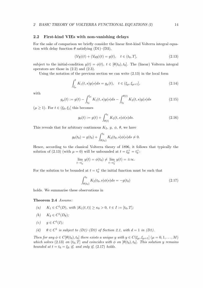
2.2 First-kind VIEs with non-vanishing delays
For the sake of comparison we briefly consider the linear first-kind Volterra integral equa-tion with delay function θ satisfying (D1)–(D3),
(Vy)(t) + (Vθy)(t) = g(t), t ∈ (t0, T ], (2.13)
subject to the initial-condition y(t) = φ(t), t ∈ [θ(t0), t0]. The (linear) Volterra integraloperators are those in (2.2) and (2.3).
Using the notation of the previous section we can write (2.13) in the local form∫ t
ξµ
K1(t, s)y(s)ds = gµ(t), t ∈ (ξµ, ξµ+1], (2.14)
with
gµ(t) := g(t)−∫ ξµ
t0K1(t, s)y(s)ds−
∫ θ(t)
t0K2(t, s)y(s)ds (2.15)
(µ ≥ 1). For t ∈ (ξ0, ξ1] this becomes
g0(t) := g(t) +∫ t0
θ(t)K2(t, s)φ(s)ds. (2.16)
This reveals that for arbitrary continuous K2, g, φ, θ, we have
g0(t0) = g(t0) +∫ t0
θ(t0)K2(t0, s)φ(s)ds 6= 0.
Hence, according to the classical Volterra theory of 1896, it follows that typically thesolution of (2.13) (with µ = 0) will be unbounded at t = ξ+
0 = t+0 :
limt→t−0
y(t) = φ(t0) 6= limt→t+0
y(t) = ±∞.
For the solution to be bounded at t = t+0 the initial function must be such that∫ t0
θ(t0)K2(t0, s)φ(s)ds = −g(t0) (2.17)
holds. We summarise these observations in
Theorem 2.4 Assume:
(a) K1 ∈ C1(D), with |K1(t, t)| ≥ κ0 > 0, t ∈ I := [t0, T ];
(b) K2 ∈ C1(Dθ);
(c) g ∈ C1(I);
(d) θ ∈ C1 is subject to (D1)–(D3) of Section 2.1, with d = 1 in (D1).
Then for any φ ∈ C[θ(t0), t0] there exists a unique y with y ∈ C(ξµ, ξµ+1] (µ = 0, 1, . . . ,M)which solves (2.13) on (t0, T ] and coincides with φ on [θ(t0), t0]. This solution y remainsbounded at t = t0 = ξ0 if, and only if, (2.17) holds.

2 BASIC THEORY OF VOLTERRA FUNCTIONAL EQUATIONS (I) 15
Is the smoothing property we encountered in solutions of delay Volterra integral equa-tions of the second kind (Theorem 2.3) also present in solutions of the first-kind delayequation (2.13)? The simple but representative example,∫ t
t0y(s)ds +
∫ θ(t)
t0λ2y(s)ds = g(t), t ∈ (t0, T ], (2.18)
with y(t) = φ(t) = φ0 for t ∈ [θ(t0), t0], whose solution can easily be found explictly, showsthat this is not so. The following theorem describes the general situation.
Theorem 2.5 Let the assumptions of Theorem 2.4 for the given functions in (2.13) hold,and assume that the initial function φ ∈ C[θ(t0), t0] is such that the solution y of theinitial-value problem for (2.13) is bounded at t = t+0 (cf. (2.17)). If y possesses a finitediscontinuity at t = t0, then it has also finite jumps at the other points of ZM .
The extension of this regularity result to first-kind Volterra integral equations andto a class of related neutral functional integro-differential equations with weakly singularkernels will play an important role in the (not yet fully understood) analysis of convergenceof collocation methods for such equations. See Brunner (1999a, 1999b) and the remarksin Section 6.3 below.
2.3 VFIDEs with non-vanishing delays
We now turn to the (regularity) properties of solutions to the the linear first-order VFIDE
y′(t) = a(t)y(t) + b(t)y(θ(t)) + g(t) + (Vy)(t) + (Vθy)(t), t ∈ I := [t0, T ], (2.19)
corresponding to the Volterra integral operators V and Vθ introduced in (2.2) and (2.3).It includes the analogue of the particular delay VIE (2.4),
y′(t) = a(t)y(t) + b(t)y(θ(t)) + g(t) + (Wθy)(t), t ∈ I, (2.20)
with Wθ given by (2.5) or (2.6).The solutions y of the VFIDE (2.19) (and hence those of (2.20)) will in general again
have lower regularity at the primary discontinuity points {ξµ} defined by the recursion
θ(ξµ) = ξµ−1, µ = 1, . . . , (ξ0 = t0)
(recall the definition and Remark preceding Theorem 2.1). We start with a basic resulton the existence and uniqueness of solutions of the initial-value problem for (2.19) (whichincludes the one for (2.20) as a particular case, corresponding to K2(t, s) = −K1(t, s) onDθ). .
Theorem 2.6 Assume:
(a) a, b, g, θ ∈ C(I), K1 ∈ C(D), K2 ∈ C(Dθ);
(b) θ(t) = t− τ(t) satisfies the conditions (D1)–(D3) of Section 2.1.
2 BASIC THEORY OF VOLTERRA FUNCTIONAL EQUATIONS (I) 16
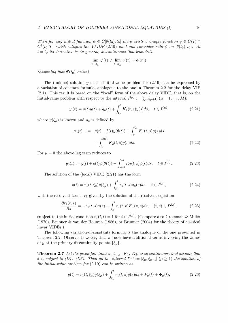
Then for any initial function φ ∈ C[θ(t0), t0] there exists a unique function y ∈ C(I) ∩C1(t0, T ] which satisfies the VFIDE (2.19) on I and coincides with φ on [θ(t0), t0]. Att = t0 its derivative is, in general, discontinuous (but bounded):
limt→t+0
y′(t) 6= limt→t−0
y′(t) = φ′(t0)
(assuming that θ′(t0) exists).
The (unique) solution y of the initial-value problem for (2.19) can be expressed bya variation-of-constant formula, analogous to the one in Theorem 2.2 for the delay VIE(2.1). This result is based on the “local” form of the above delay VIDE, that is, on theinitial-value problem with respect to the interval I(µ) := [ξµ, ξµ+1] (µ = 1, . . . ,M):
y′(t) = a(t)y(t) + gµ(t) +∫ t
ξµ
K1(t, s)y(s)ds, t ∈ I(µ), (2.21)
where y(ξµ) is known and gu is defined by
gµ(t) := g(t) + b(t)y(θ(t)) +∫ ξµ
t0K1(t, s)y(s)ds
+∫ θ(t)
t0K2(t, s)y(s)ds. (2.22)
For µ = 0 the above lag term reduces to
g0(t) := g(t) + b(t)φ(θ(t))−∫ t0
θ(t)K2(t, s)φ(s)ds, t ∈ I(0). (2.23)
The solution of the (local) VIDE (2.21) has the form
y(t) = r1(t, ξµ)y(ξµ) +∫ t
ξµ
r1(t, s)gµ(s)ds, t ∈ I(µ), (2.24)
with the resolvent kernel r1 given by the solution of the resolvent equation
∂r1(t, s)∂s
= −r1(t, s)a(s)−∫ t
sr1(t, v)K1(v, s)dv, (t, s) ∈ D(µ), (2.25)
subject to the initial condition r1(t, t) = 1 for t ∈ I(µ). (Compare also Grossman & Miller(1970), Brunner & van der Houwen (1986), or Brunner (2004) for the theory of classicallinear VIDEs.)
The following variation-of-constants formula is the analogue of the one presented inTheorem 2.2. Observe, however, that we now have additional terms involving the valuesof y at the primary discontinuity points {ξµ}.
Theorem 2.7 Let the given functions a, b, g, K1, K2, φ be continuous, and assume thatθ is subject to (D1)–(D3). Then on the interval I(µ) := [ξµ, ξµ+1] (µ ≥ 1) the solution ofthe initial-value problem for (2.19) can be written as
y(t) = r1(t, ξµ)y(ξµ) +∫ t
ξµ
r1(t, s)g(s)ds + Fµ(t) + Φµ(t), (2.26)

2 BASIC THEORY OF VOLTERRA FUNCTIONAL EQUATIONS (I) 17
with
Fµ(t) :=µ−1∑ν=1
ρµ,ν(t)y(ξν) +∫ ξ1
ξ0rµ,0(t, s)g0(s)ds +
µ−1∑ν=1
∫ ξν+1
ξν
rµ,ν(t, s)g(s)ds,
Φµ(t) :=∫ θµ(t)
ξ0qµ,0(t, s)g0(s)ds +
µ−1∑ν=1
∫ θµ−ν(t)
ξν
qµ,ν(t, s)g(s)ds.
On the first interval I(0) this representation reduces to
y(t) = r1(t, t0)y(t0) +∫ t
t0r1(t, s)g0(s)ds, (2.27)
where y(t0) = φ(t0). The functions ρµ,ν , rµ,ν , and qµ,ν depend on a, b, K1, K2, r1 and θand are continuous on their respective domains; r1 = r1(t, s) denotes the resolvent kernelfor K1 = K1(t, s) defined by the resolvent equation (2.25).
Proof: The basic idea governing the proof of the above result is essentially the one usedto establish Theorem 2.2, except that now the variation-of-constant formula is based onthe resolvent representation of the solution of the “local” VIDE (2.21) and will thus reflectthe initial values y(ξµ). We leave the details of this simple proof to the reader.
Remarks:
1. As in Theorem 2.2 we see again how the presence of the delay term (Vθy)(t) in (2.19)influences the resolvent representation of the classical (non-delay) VIDE on themacro-interval I(µ). In addition, we have now terms reflecting the initial-valuesy(ξν) (0 ≤ ν ≤ µ).
2. There is a close connection between the representation of the solution of certain classesof Volterra functional (integro-) differential equations and the semigroup frameworkinto which such equations can be embedded. Among the many papers dealing withthis framework and corresponding solution representations we mention Burns, Herd-man & Stech (1983c), Staffans (1985a, 1985b), Kappel & Zhang (1986), Burns, Herd-man & Turi (1987), Clement, Desch & Homan (2002), and Ito & Kappel (2002).
2.4 Volterra functional equations with weakly singular kernels
As we have briefly seen in the remarks following equation (1.10), Volterra functional inte-gral and integro-differential equations with weakly singular (i.e. unbounded but integrable)kernels occur in many applications. Due to limitations of space we shall not be able to saymuch about them in this paper, except for some brief remarks in(Section 6.1. Here, weintroduce relevant notation and point to papers in which the reader will find additionalinformation.
Assume that α ∈ (0, 1) is given, and define the delay integral operators
(Vθ,αy)(t) :=∫ θ(t)
0(t− s)−αK(t, s)y(s)ds, (2.28)

2 BASIC THEORY OF VOLTERRA FUNCTIONAL EQUATIONS (I) 18
and(Wθ,αy)(t) :=
∫ t
θ(t)(t− s)−αK(t, s)y(s)ds, (2.29)
corresponding to continuous kernel functions K satisfying |K(t, t)| ≥ k0 > 0 when s = t. InSection 6.2 we will comment on some of the open problems arising when the correspondingfunctional equations
y(t) = g(t) + (Tθ,αy)(t) (2.30)
andy′(t) = f(t, y(t), y(θ(t))) + (Tθ,αy)(t), (2.31)
with Tθ,α representing one of the Volterra integral operators Vθ,α or Wθ,α.In Section 1.2 (equation (1.10)) We have encountered a (system of a) functional integro-
differential equations of neutral type whose scalar counterpart may be written as (usingnow our standard notation),
d
dt[a0y(t)− (Wθ,αy)(t)] = F (t, y(t), y(θ(t)), y′(θ(t))), t ≥ 0,
with 0 < α < 1 and
(Wθ,αy)(t) :=∫ t
θ(t)(t− s)−αK(t, s)y(s)ds, θ(t) = t− τ.
A related (but more complex) Volterra functional integro-differential equation is
d
dt[(Wθ,αy)(t)] = f(t). (2.32)
The mathematical analysis of functional equations of this type may be found in, e.g.,Kappel & Zhang (1986), Ito & Kappel (1991), Clement, Desch & Homan (2002), andIto & Kappel (2002). We will briefly return to these two classes of functional equationsin Section 6.1. The mathematical (semigroup) framework for such equations has beendeveloped in, e.g., the papers and the monograph mentioned at the end of Section 2.3(Remark 2); results on the regularity of their solutions may be found in Brunner & Ma(2006).

3 COLLOCATION METHODS FOR VFES WITH NON-VANISHING DELAYS 19
3 Collocation methods for VFEs with non-vanishing delays
3.1 Numerical analysis of VFEs: an overview
We will use this section to sketch briefly the development of numerical methods for solvingdelay differential equations and more general functional integral and integro-differentialequations of Volterra type. In the subsequent sections we shall then focus on collocationmethods for such problems.
Most of the early discretisation schemes for delay problems are based on “classical”linear multistep and Runge-Kutta methods for ODEs. These methods have to be com-plemented by a suitable interpolation procedure (e.g. by a natural continuous extension(NCE)), to generate approximations at certain non-mesh points θ(t). One of the principalmerits of a collocation method is that the NCE is part of the method itself.
3.1.1 DDEs
The monograph by Myshkis (1951) (in Russian; see also the German translation of 1955and the second (Russian) edition of 1972) stands at the beginning of a sequence of dis-tinguished monographs on the theory and applications of delay differential equations. Ofthese we mention Bellman & Cooke (1964), El’sgol’ts & Norkin (1973), Hale (1977), Kol-manovskii & Myshkis (1992), Hale & Verduyn Lunel (1993), Diekmann et al. (1993), Wu(1996) (on partial DDEs), and Ito & Kappel (2002) (on more general functional equations).The early survey papers by Halanay & Yorke (1971), Cryer (1972) and Bellen (1985), whenread in “hand-in-hand” with the recent ones by Zennaro (1995), Baker (1997, 2000), Baker& Paul (1997), Bocharov & Rihan (2000) and Bellen, Guglielmi & Maset (2006) give agood idea of how the interest in theory, numerical analysis, and applications of DDEs hasgrown since the early 1970s.
The monograph by Bellen & Zennaro (2003) provides not only a good introduction,also by means of numerous illuminating examples, to the theory of DDEs but gives astate-of-the-art treatment of numerical methods for DDEs. Focusing on Runge-Kuttatype methods, we see that, beginning in the early 1980s, one can discern two main trendsin the analysis of such methods: the first is concerned with the adaptation of (explicit andimplicit) RK methods to DDEs and the construction of various interpolants, includingNCEs. Typical contributions are the ones by Bellen & Zennaro (1985), Zennaro (1986), in’t Hout (1992), and Vermiglio & Zennaro (1993). Chapters 5 and 6 in Bellen & Zennaro(2003) contain a description of these quantitative aspects. Computatinal aspects arediscussed in detail in Bellen & Zennaro (2003); compare also Neves & Thompson (1992),Baker, Paul & Wille (1995), Guglielmi & Hairer (2001b) and Feldstein, Neves & Thompson(2006).
The second aspect is the study of asymptotic stability and contractivity properties ofRK methods. Early milestones in the qualitative analysis of such methods are the papersby Reverdy (1981, 1990) and Torelli (1989). The reader may also wish to consult, ofthe many later contributions extending these results, the ones by Zennaro (1993, 1997),Torelli & Vermiglio (1993), Spijker (1997), Guglielmi (1998, 2001) (dealing with delay-dependent stability), Guglielmi & Hairer (2001a), Maset (2002a), and Vermiglio & Torelli(2003). However, in these lectures we shall not deal with qualitative properties of numerical

3 COLLOCATION METHODS FOR VFES WITH NON-VANISHING DELAYS 20
solutions to VFIEs and VFIDEs (compare also Section 6.5), except for observing thatthe analysis of the qualitative behaviour of collocation solutions for VFIEs and VFIDEsremains largely open.
Most of these papers consider only DDEs with constant delay τ > 0. For general lagfunctions θ(t) = t− τ(t) with nonlinear delay τ(t), the analysis and the implementation ofIRK methods become much more complex (compare Lemma 3.1 below). This problem isnot present in piecewise polynomial collocation methods since, as we have indicated before,they are global methods and thus automatically imclude a NCE. Bellen (1984) gave thefirst complete (super-) convergence analysis for such methods when applied to nonlinearDDEs with general nonlinear (non-vanishing) delays; his analysis is complemented inVermiglio (1985). These collocation methods employ distinct collocation points; Hermite-type collocation for DDEs (and the attainable order of convergence) was studied by Oberle& Pesch (1981). More recent work on various aspects of collocation methods are studied inEnright & Hayashi (1998), Liu (1999a, 1999b), Engelborghs et al. (2000), Engelborghs &Doedel (2002), and in Guglielmi & Hairer (2001a) (introducing the powerful DDE softwareRADAR5 based on collocation at Radau II points).
We will not mention any of the superconvergence results here, since they can be ob-tained as particular cases of the ones for Volterra-integro-differential equations with delays(see Section 3.5).
3.1.2 VFIEs of the second kind
As we saw in Section 1, the first papers on the theory of delay integral equations (Volterra(1997), Lalesco (1908, 1911), and Andreoli (1913, 1914)) considered the case of vanishing(proportional) delays. The development of the early theory for Volterra equations withnon-vanishing delays is well sketched in Vogel (1965). Of interest is also the paper by Lin(1963) which contains a comparison result for solutions of systems of second-kind Volterraintegral equations with constant delay. Additional results on the existence, uniqueness,and representation of solutions to such functional equations can be found in Levin &Nohel (1964), Bownds, Cushing & Schutte (1976), Cerha (1976), Muresan (1984, 1999),as well as in Cooke (1976), Esser (1976, 1978), Meis (1976), Busenberg & Cooke (1980),Cahlon, Nachman & Schmidt (1984) and Canada & Zertiti (1994) (see also for additionalreferences). Chapter 4 in Brunner (2004) contains an introduction to the theory of VFIEsand VFIDEs with non-vanishing delays.
The numerical analysis of Volterra integral equations with delays can be traced backto Esser (1976, 1978), Vata (1978), Wolff (1982), and Cahlon et al. (1984, 1985). Morerecent contributions on Runge-Kutta methods are by Arndt & Baker (1988), Baker &Derakhshan (1990), Vermiglio (1992), as well as by Cahlon (1990, 1992, 1995), Cahlon &Schmidt (1997), and Tian & Kuang (1995) (on the stability of numerical approximations).The reader may also wish to look at the survey papers by Cryer (1972) and Baker (1997,2000).
Collocation methods in piecewise polynomial spaces occur in Vermiglio (1992), andtheir superconvergence properties are studied in detail in Brunner (1994a), Baddour &Brunner (1995), Hu (1997, 1999), and Brunner (2004a) (Chapter 4). The reader may alsowish to consult the recent survey paper by Brunner (2008a).

3 COLLOCATION METHODS FOR VFES WITH NON-VANISHING DELAYS 21
3.1.3 VFIDEs
The literature on the theory and the numerical solution of VIDEs with delays is moreextensive. It starts of coure with Volterra’s work (Volterra (1909, 1912) and, especially,(1927, 1931)). Of the numerous books we list the ones by Cushing (1977), Gyori & Ladas(1991), Lakshmikantham, Wen & Zhang (1994), Ito & Kappel (2002), and Zhao (2003);see also the surveys by Corduneanu & Lakshmikantham (1980) and Jackiewicz & Kwapisz(1991), and their bibliographies. The regularity of solutions is analysed in, e.g., Wille& Baker (1992), Brunner & Zhang (1999) Baker & Wille (2000), and in Brunner & Ma(2006).
Important early contributions to the numerical solution of VFIDEs are due to Thomp-son (1968) and Tavernini (1971, 1973, 1978) (linear multistep and general one-step meth-ods). We also mention the papers by Jackiewicz (1981), Arndt & Baker (1988), Jackiewicz& Kwapisz (1991), Makroglou (1983) (block methods for VIDEs with constant delay),Kazanova & Bainov (1990), Enright & Hu (1997) (continuous Runge-Kutta methods),and Baker & Tang (1997, 2000). Most of these methods are based on ODE schemes andhence they require an appropriate interpolation scheme to produce “dense” data. Theconstruction of NCEs for RK methods applied to classical VIDEs is the subject in Ver-miglio (1988) (see also Bellen, Jackiewicz, Vermiglio & Zennaro (1989) for the case ofdelay VIEs); it can be extended to VIDEs with non-vanishing delays. Bellen (1985) andBaker (1997, 2000) contain comprehensive surveys and extensive lists of references on thenumerical treatment of functional differential equations.
The numerical treatment of partial VFIDEs have received increased attention in recentyears. This topic is beyond the scope of this articel (and the expertise of its author); theinterested reader may consult Zubik-Kowal (1999) and Zubik-Kowal & Vandewalle (1999)for results and additional references.
Cryer & Tavernini (1972) study Euler’s method for very general Volterra functionalequations. This method may of course be interpreted as a simple collocation method. The(super-) convergence properties of piecewise polynomial collocation methods for VFIDEsare described in Brunner (1994b), Burgstaller (1993, 2000), and Hu & Peng (1999); seealso Chapter 4 in Brunner (2004). The papers by Koto (2002) and by Brunner & Vermiglio(2003) investigate stability and contractivity properties of solutions to VFIDEs with con-stant delays and neutral VFIDEs of “Hale’s form”. However, much work remains to bedone before a good understanding of the qualitative (asymptotic) properties of collocationsolutions to general (nonlinear) VFIDEs is obtained.
Finally, we mention another, important approach to the numerical solution of VFIDEs:it is based on a semi-group framework generated by the given functional equation (cf. alsoClement, Desch & Homan (2002) and references) and is able to deal with a rather generalclass of (linear) neutral VFIDEs. This approach originated in the work of Banks & Kappel(1979); see also Ito & Kappel (1989, 1991), Ito & Turi (1991), Clement, Desch & Homan(2002) and, especially, the recent monograph by Ito & Kappel (2002).
3.2 Collocation methods for VFIEs with non-vanishing delays
In order to lead the reader not familiar with collocation methods for classical Volterraintegral and integro-differential equations to their application to Volterra-type functional

3 COLLOCATION METHODS FOR VFES WITH NON-VANISHING DELAYS 22
equations, we briefly summarise the principal ideas and mathematical tools underlyingthese global discretisation methods.
3.2.1 Collocation spaces for classical Volterra equations
Let Ih := {tn : 0 = t0 < t1 < · · · < tN = T} be a mesh on the interval I := [0, T ], andset
σn := (tn, tn+1], σn := [tn, tn+1], hn := tn+1 − tn (0 ≤ n ≤ N − 1);
the diameter of the mesh Ih is h := max(n) hn. For given integers m ≥ 1 and d ≥ −1 wedenote by
S(d)m+d(Ih) := {uh ∈ Cd(I) : uh|σn ∈ πm+d (0 ≤ n ≤ N − 1)} (3.1)
the linear space of (real) piecewise polynomials with respect to the mesh Ih whose degreedoes not exceed m + d. If d = −1 then uh ∈ S
(−1)m−1(Ih) will in general have finite (jump)
discontinuities at the interior points of Ih; the space of step functions, S(−1)0 (Ih), is the
most obvious example of such a discontinuous piecewise polynomial space.The dimension of the linear space defined by (3.1) is given by
dim S(d)m+d(Ih) = Nm + (d + 1).
The choice of d, the degree of regularity, will be governed by the type of functional equationwhose solution will be approximated by collocation in the linear space S
(d)m+d(Ih): for
the functional integral equations not containing derivatives of the unknown solution the“natural” piecewise polynomial space is S
(−1)m−1(Ih) (d = −1), while for functional integro-
differential equations in which the highest derivative of the unknown solution is y(k) (k ≥ 1)we choose d = k − 1.
The desired collocation solution uh ∈ S(d)m+d(Ih) will be determined by requiring that
it satisfy the given functional equation on the set of collocation points
Xh := {tn,i := tn + cihn : 0 < c1 < · · · < cm ≤ 1 (0 ≤ n ≤ N − 1)}, (3.2)
described by given collocation parameters {ci}. Clearly,
dim S(d)m+d(Ih) = Nm + (d + 1) = |Xh|+ (d + 1).
If d ≥ 0 the collocation solution will also be required to concide, at t = 0, with theprescribed initial value(s); e.g., in the case of the DVIDEs (2.19) and (2.20) (k = 1) wehave uh(0) = y0.
3.2.2 Constrained and θ-invariant meshes
Assume that the given lag function θ(t) = t− τ(t) satisfies the assumptions (D1)–(D3) ofSection 2.1 which we will recall for the convenience of the reader:
(D1) θ(t) = t− τ(t), with τ(t) ≥ τ0 > 0 for t ∈ I;
(D2) θ is strictly increasing on I;

3 COLLOCATION METHODS FOR VFES WITH NON-VANISHING DELAYS 23
(D3) τ ∈ Cd(I) for some d ≥ 0.
We have seen (see the comments preceding Theorem 2.1) that the primary discontinuitypoints {ξµ}, induced by θ and given by θ(ξµ) = ξµ−1 (µ = 1, . . . ; ξ0 := t0), possess the(uniform) separation property
ξµ − ξµ−1 ≥ τ0 > 0 for all µ ≥ 1.
For ease of notation we will again assume that T defining I = [t0, T ] is such that
T = ξM+1 for some M ≥ 1,
and we set ZM := {ξµ : µ = 0, 1, . . . ,M}.Since solutions of delay problems with non-vanishing delays generally suffer from a
loss of reguarity at the primary discontinuity points {ξµ}, the mesh Ih underlying thecollocation space will have to include these points if the collocation solution is to attainits optimal global (or local) order (of superconvergence. Thus, we shall employ meshes ofthe form
Ih :=M⋃
µ=0
I(µ)h , I
(µ)h := {t(µ)
n : ξµ = t(µ)0 < t
(µ)1 < . . . < t
(µ)Nµ
= ξµ+1}. (3.3)
Such a mesh is called a constrained mesh (with respect to θ) for I. We will refer to Ih asthe macro-mesh and call the I
(µ)h the underlying local meshes (compare also Bellen (1984,
1985)).
Definition 3.1:A mesh Ih for I := [t0, T ] is said to be θ-invariant if it is constrained (that is, given by(3.3)) and if
θ(I(µ)h ) = I
(µ−1)h (µ = 1, . . . ,M) (3.4)
holds. We then have Nµ = N for all µ ≥ 0.
Observe that if Ih is θ-invariant then
t ∈ I(µ)h =⇒ θµ−ν(t) ∈ I
(ν)h (ν = 0, 1, . . . , µ). (3.5)
In analogy to Section 3.2.1 we will use the following notation:
σ(µ)n := (t(µ)
n , t(µ)n+1], h(µ)
n := t(µ)n+1 − t(µ)
n , h(µ) := max(n)
h(µ)n , h := max
(µ)h(µ),
and σ(µ)n := [t(µ)
n , t(µ)n+1].
For a given θ-invariant mesh Ih the collocation solution uh will be an element of apiecewise polynomial space
S(d)m+d(Ih) := {v ∈ Cd(Ih) : v|
σ(µ)n
∈ πm+d (0 ≤ n < N ; 0 ≤ µ ≤ M)}. (3.6)
It follows from Section 3.2.1 that this linear space has the dimension
dim S(d)m+d(Ih) = (M + 1)Nm + d + 1.

3 COLLOCATION METHODS FOR VFES WITH NON-VANISHING DELAYS 24
Hence the collocation points will now be chosen as
Xh :=M⋃
µ=0
X(µ)h ; (3.7)
they are based on the M + 1 local sets
X(µ)h := {t(µ)
n + cih(µ)n : 0 < c1 < . . . < cm ≤ 1 (0 ≤ n ≤ N − 1)}
of cardinality Nm. In the collocation equation for a given delay equation with non-vanishing delay τ(t) we shall encounter the mapping θ(X(µ)
h ) (see, for example, (3.9)below). It is clear that for linear lag functions θ and given θ-invariant mesh Ih the setXh defined by (3.7) is also θ-invariant. However, for nonlinear delays this will no longerbe true. We record this important fact – which will affect the computational form of thecollocation equation – in the following lemma. Its proof is straightforward and is left asan exercise.
Lemma 3.1 Assume that the delay function θ satisfies (D1)–(D3), and let Ih be a θ-invariant mesh on I = [t0, T ].
(a) If θ is linear, thenθ(X(µ)
h ) = X(µ−1)h , µ = 1, . . . ,M :
the set Xh of collocation points is also θ-invariant.
(b) For nonlinear θ this is no longer true: setting
θ(t(µ)n + cih
(µ)n ) = t(µ−1)
n + cih(µ−1)n =: t
(µ−1)n,i (i = 1, . . . ,m),
the images {ci} of the {ci} satisfy
0 ≤ c1 < . . . < cm ≤ 1 (with ci 6= ci in general),
and they depend on the micro-interval σ(µ)n and on the macro-interval I(µ):
ci = ci(n;µ) (i = 1, . . . ,m).
3.3 VFIEs of the second kind
3.3.1 The collocation equations
The collocation solution uh ∈ S(−1)m−1(Ih) for the delay integral equation
y(t) = g(t) + (Vy)(t) + (Vθy)(t), t ∈ (t0, T ], (3.8)
with
(Vy)(t) :=∫ t
t0K1(t, s)y(s)ds, (Vθy)(t) :=
∫ θ(t)
t0K2(t, s)y(s)ds,

3 COLLOCATION METHODS FOR VFES WITH NON-VANISHING DELAYS 25
and with initial condition y(t) = φ(t), t ≤ t0, is defined by the collocation equation
uh(t) = g(t) + (Vuh)(t) + (Vθuh)(t), t ∈ Xh. (3.9)
The values of uh at t ∈ [θ(t0), t0] are determined by the given initial function for (3.8),uh(t) = φ(t). As for classical second-kind Volterra integral equations we will also considerthe iterated collocation solution corresponding to uh:
uith (t) := g(t) + (Vuh)(t) + (Vθuh)(t), t ∈ (t0, T ]. (3.10)
The lag function θ = θ(t) = t−τ(t) will be assumed to satisfy the conditions (D1)–(D3) ofSection 3.2.2, and the mesh Ih on I := [t0, T ] will be assumed to be the θ-invariant meshdefined by (3.3) and (3.4).
On σ(µ)n := (t(µ)
n , t(µ)n+1] the collocation solution will have the usual local Lagrange
representation,
uh(t(µ)n + vh(µ)
n ) =m∑
j=1
Lj(v)U (µ)n,j , v ∈ (0, 1], with U
(µ)n,j := uh(t(µ)
n,j). (3.11)
Since the contribution of the classical Volterra term Vuh to the computational form ofthe collocation equation is obvious we will focus here on the terms induced by the delaypart (Vθuh)(t) with t = t
(µ)n,i .
Assume first that the delay θ is linear. Since, as we have seen in Lemma 3.1, theθ-invariance of the mesh Ih implies the θ-invariance of the set Xh of collocation points, wemay write, using the fact that θ(t(µ)
n,i ) = t(µ−1)n,i ,
(Vθuh)(t(µ)n,i ) =
∫ θ(t(µ)n,i )
t0K2(t
(µ)n,i , s)uh(s)ds =
∫ t(µ−1)n,i
t0K2(t
(µ)n,i , s)uh(s)ds, (3.12)
and hence, recalling the local representation (3.11) of uh,
(Vθuh)(t(µ)n,i ) = Ψ(µ−1)
n (t(µ)n,i ) +
h(µ−1)n
m∑j=1
(∫ ci
0K2(t
(µ)n,i , t
(µ−1)n + sh(µ−1)
n )Lj(s)ds
)U
(µ−1)n,j , (3.13)
with lag term
Ψ(µ−1)n (t) :=
∫ ξµ−1
t0K2(t, s)uh(s)ds +
∫ t(µ−1)n
ξµ−1
K2(t, s)uh(s)ds (t ∈ σ(µ)n ). (3.14)
If the delay θ is nonlinear, then the above terms have to be modified: by the (strict)monotonicity assumption (D3) for θ the image of t
(µ)n,i ∈ σ
(µ)n under θ lies in σ
(µ−1)n (but
will be different from the collocation point t(µ−1)n,i = t
(µ−1)n + cih
(µ−1)n ); that is,
θ(t(µ)n,i ) = t(µ−1)
n + cih(µ−1)n =: t
(µ−1)n,i (i = 1, . . . ,m), (3.15)
with0 < c1 < . . . < cm ≤ 1 and ci = ci(n;µ)
3 COLLOCATION METHODS FOR VFES WITH NON-VANISHING DELAYS 26
(cf. Lemma 3.1). Accordingly, the expression (3.13) for (Vθuh)(t(µ)n,i ) now reads
(Vθuh)(t(µ)n,i ) = Ψ(µ−1)
n (t(µ)n,i ) +
h(µ−1)n
m∑j=1
(∫ ci
0K2(t
(µ)n,i , t
(µ−1)n + sh(µ−1)
n )Lj(s)ds
)U
(µ−1)n,j . (3.16)
Hence, the collocation equation (3.9) at t = t(µ)n,i (i = 1, . . . ,m) can now be written as
U(µ)n,i = h(µ)
n
m∑j=1
(∫ ci
0K1(t
(µ)n,i , t
(µ)n + sh(µ)
n )Lj(s)ds
)U
(µ)n,j (3.17)
+g(t(µ)n,i ) + F (µ)
n (t(µ)n,i ) + (Vθuh)(t(µ)
n,i ).
The classical lag term (corresponding to the Volterra operator V in (3.9)) has, for t ∈ σ(µ)n ,
the form
F (µ)n (t) :=
∫ ξµ
t0K1(t, s)uh(s)ds +
∫ t(µ)n
ξµ
K1(t, s)uh(s)ds (3.18)
Let U(µ)n := ( U
(µ)n,1 , . . . , U
(µ)n,m )T ∈ IRm and define the matrices in L(IRm),
B(µ)n :=
∫ ci
0K1(t
(µ)n,i , t
(µ)n + sh
(µ)n )Lj(s)ds
(i, j = 1, . . . ,m)
,
B(µ−1)n :=
∫ ci
0K2(t
(µ)n,i , t
(µ−1)n + sh
(µ−1)n )Lj(s)ds
(i, j = 1, . . . ,m)
.
Finally, set g(µ)n := ( g(t(µ)
n,1), . . . , g(t(µ)n,m) )T , G(µ)
n := ( F (t(µ)n,1), . . . , F
(µ)n (t(µ)
n,m )T , and
Q(µ−1)n := ( Ψ(µ−1)
n (t(µ)n,1), . . . ,Ψ
(µ−1)n (t(µ)
n,m) )T .
Thus, the collocation solution uh ∈ S(−1)m−1(Ih) to (3.8) on σ
(µ)n is described by (3.11) in
which U(µ)n is the solution of the linear algebraic system
[Im − h(µ)n B(µ)
n ]U(µ)n = g(µ)
n + G(µ)n + Q(µ−1)
n + h(µ−1)n B(µ)
n U(µ−1)n (3.19)
(n = 0, 1, . . . ,m; µ = 0, 1, . . . ,M). The matrix Im denotes the identity operator in L(IRm).The following theorem on the existence of a unique collocation solution is an obvious
consequence of the uniform boundedness of the inverses of the matrices B(µ)n := Im −
h(µ)n B
(µ)n for sufficiently small mesh diameters h.
Theorem 3.2 Assume that g, θ, K1 and K2 are continuous on their respective domainsI, D and Dθ, with the lag function θ satisfying (D1)–(D3).Then there exists an h > 0 so that for any θ-invariant mesh Ih with h ∈ (0, h) andany initial function φ ∈ [θ(t0), t0] each of the linear algebraic systems (3.19) possessesa unique solution U(µ)
n ∈ IRm. Hence, the collocation equation (3.9) defines a uniquecollocation solution uh ∈ S
(−1)m−1(Ih) for (3.8) whose local representation on the subintervals
σ(µ)n is given by (3.11).

3 COLLOCATION METHODS FOR VFES WITH NON-VANISHING DELAYS 27
The computational form of the iterated collocation solution (3.10) at t = t(µ)n + vh
(µ)n ∈
σ(µ)n can be written as
uith (t) = g(t) + F (µ)
n (t) + Ψ(µ−1)n (t)
+h(µ)n
m∑j=1
(∫ v
0K1(t, t(µ)
n + sh(µ)n )Lj(s)ds
)U
(µ)n,j (3.20)
+h(µ−1)n
m∑j=1
(∫ v
0K2(t, t(µ−1)
n + sh(µ−1)n )Lj(s)ds
)U
(µ−1)n,j .
Recall that the lag term Ψ(µ−1)n (t) corresponding to the delay operator Vθ is given above
by (3.14). The image t := t(µ−1)n + vh
(µ−1)n of t = t
(µ)n + vh
(µ)n under θ depends on the
nature of the lag function θ: if θ is linear then we have v = v; for nonlinear θ the value ofv ∈ [0, 1] must be obtained from
θ(t(µ)n + vh(µ)
n ) =: t(µ−1)n + vh(µ−1)
n , v ∈ (0, 1]. (3.21)
We note in passing that uith ∈ C[t0, T ] whenever the given data defining the initial-value
problem for (3.8) are continuous functions and we have
uith (t0) = g(t0)−
∫ t0
θ(t0)K2(t0, s)φ(s))ds ( = y(t+0 ) ).
Moreover,uit
h (t) = uh(t) for all t ∈ Xh.
Since second-kind VFIEs with non-vanishing delays often arise in the particular form
y(t) = g(t) + (Wθy)(t), t ∈ (t0, T ], (3.22)
where(Wθy)(t) :=
∫ t
θ(t)K(t, s)y(s)ds,
we present the corresponding computational form of the collocation equation defininguh ∈ S
(−1)m−1(Ih) in some detail (although it could of course be formally obtained by setting
K2 = −K1 =: −K in (3.17). We first note that for t = t(µ)n,i we have
(Wθuh)(t) =∫ t
(µ−1)n+1
θ(t)K(t, s)uh(s)ds
+∫ ξµ
t(µ−1)n+1
K(t, s)uh(s)ds +∫ t
(µ)n
ξµ
K(t, s)uh(s)ds (3.23)
+h(µ)n
∫ ci
0K(t, t(µ)
n + sh(µ)n )uh(t(µ)
n + sh(µ)n )ds,
where
θ(t) = θ(t(µ)n,i ) =
{t(µ−1)n,i = t
(µ−1)n + cih
(µ−1)n if θ is linear,
t(µ−1)n,i := t
(µ−1)n + cih
(µ−1)n if θ is nonlinear.
.

3 COLLOCATION METHODS FOR VFES WITH NON-VANISHING DELAYS 28
Define, for t = t(µ)n + cih
(µ)n ,
Ψ(µ−1)n (t) := h(µ−1)
n
∫ 1
ci
K(t, t(µ−1)n + sh(µ−1)
n )uh(t(µ−1)n + sh(µ−1)
n )ds
+∫ ξµ
t(µ−1)n+1
K(t, s)uh(s)ds +∫ t
(µ)n
ξµ
K(t, s)uh(s)ds. (3.24)
The collocation equation for (3.22) on σ(µ)n then becomes
U(µ)n,i = g(t(µ)
n,i ) + Ψ(µ−1)n (t(µ)
n,i ) +
h(µ)n
m∑j=1
(∫ ci
0K(t(µ)
n,i , t(µ)n + sh(µ)
n )Lj(s)ds
)U
(µ)n,j (i = 1, . . . ,m). (3.25)
Hence, the resulting linear algebraic system for U(µ)n ∈ IRm defining the local representation
of uh on σ(µ)n (cf. (3.11)) has the form
[Im − h(µ)n B(µ)
n ]U(µ)n = g(µ)
n + G(µ−1)n , (3.26)
with g(µ)n := ( g(t(µ)
n,1, . . . , g(t(µ)n,m )T and G(µ−1)
n := ( Ψ(µ−1)n (t(µ)
n,1), . . . , Ψ(µ−1)n (t(µ)
n,m) )T .
The corresponding iterated collocation solution at t = t(µ)n + vh
(µ)n ∈ σ
(µ)n can be then
computed via
uith (t) = g(t) + Ψ(µ−1)
n (t)
+h(µ)n
m∑j=1
(∫ ci
0K(t, t(µ)
n + sh(µ)n )Lj(s)ds
)U
(µ)n,j . (3.27)
We note that in applications uith (t) will only be computed for special values of t, for example
for t = tN = T , or t = ξµ (cf. Theorem 3.6 and Corollaries 3.7 and 3,8).
3.3.2 Global convergence results
The collocation error eh := y− uh associated with the collocation solution uh ∈ S(−1)m−1(Ih)
for the VFIE (3.8) solves the initial-value problem
eh(t) = δh(t) + (Veh)(t) + (Vθeh)(t), t ∈ (t0, T ], (3.28)
with initial condition eh(t) = 0 for t ∈ [θ(t0), t0]. The defect δh, defined by
δh(t) := −uh(t) + g(t) + (Vuh)(t) + (Vθuh)(t), t ∈ I,
vanishes on the set Xh. For t ∈ σ(µ)n (µ ≥ 1) the above error equation can be written as
eh(t) = Eµ(t) + δh(t) +∫ t
ξµ
K1(t, s)eh(s)ds, (3.29)

3 COLLOCATION METHODS FOR VFES WITH NON-VANISHING DELAYS 29
where
Eµ(t) :=µ−1∑ν=0
∫ ξν+1
ξν
K1(t, s)eh(s)ds + (Vθeh)(t). (3.30)
On the first macro-interval (t0, ξ1] we have
E0(t) := (Vθeh)(t) = −∫ t0
θ(t)K2(t, s)eh(s)ds = 0.
If the given functions in (3.8) have continuous derivatives of at least order m on theirrespective domains, the global convergence and order analysis can be based on the (local)representation of the collocation error based on the Peano Kernel Theorem for polynomialinterpolation. This representation has the form
eh(t(µ)n + vh(µ)
n ) =m∑
j=1
Lj(v)E(µ)n,j + (h(µ)
n )mR(µ)m,n(v), v ∈ (0, 1], (3.31)
with E(µ)n,j := eh(t(µ)
n,j) and Peano remainder term R(µ)m,n(v) (see Brunner (2004), Chapters 1
and 2, for details). On the first macro-interval [ξ0, ξ1] the estimate for eh is the one forclassical Volterra integral equations of the second kind (Brunner & van der Houwen (1986)(Chapter 5):
||eh||0,∞ := supt∈I(0)
|eh(t)| ≤ C0(h(0))m (n = 0, 1, . . . , N − 1);
it is a consequence of the estimate ||E(0)n ||1 = O((h(0))m) (where E(µ)
n := ( E(µ)n,1 , . . . , E(µ)
n,m )T ).A simple induction argument, employing the estimates for the terms Eµ(t) (t ∈ I(µ)) in(3.29) and (3.30), together with the observation that by the conditions (D1)–(D3) for thedelay θ the number (M +1) of macro-intervals I(µ) := [ξµ, ξµ+1] is finite, yields the resultssummarised in the following theorem.
Theorem 3.3 Assume:
(a) The given functions g, K1, K2 and φ in (3.8) all possess continuous derivatives oforder m on their respective domains.
(b) The delay function θ(t) = t− τ(t) is subject to the conditions (D1)–(D3) of Section3.2.2, with d ≥ m in (D1).
(c) uh ∈ S(−1)m−1(Ih) is the collocation solution to (4.8) corresponding to a θ-invariant
mesh Ih with h ∈ (0, h, where h is defined in Theorem 3.2.
Then for any set of collocation parameters {ci : 0 ≤ c1 < . . . < cm ≤ 1} the collocationerror admits the estimate
||y − uh||∞ := supt∈(t0,T ]
|eh(t)| ≤ Chm. (3.32)
The constant C depends on the {ci} but not on h := max(n,µ) h(µ)n .

3 COLLOCATION METHODS FOR VFES WITH NON-VANISHING DELAYS 30
Although it follows from (3.28) and Theorem 3.3 that, in general, ||δh||∞ = O(hm)only, a judicious choice of the collocation parameters {ci} leads (not too surprisingly, ifwe look at the close connection between the degree of precision of interpolatory m-pointquadrature formulas based on these abscissas and the variation-of-constants formula ofTheorem 2.2 adapted to the error equation!) to global superconvergence on I for theiterated collocation solution uit
h .
Theorem 3.4 Suppose that the assumptions (a)–(c) of Theorem 3.3 hold, but with m+1replacing m in (a) and (b). If the collocation parameters {ci} are chosen so that theorthogonality condition
J0 :=∫ 1
0
m∏i=1
(s− ci) ds = 0 (3.33)
is satisfied, then the iterated collocation solution corresponding to the collocation solutionuh ∈ S
(−1)m−1(Ih) for (3.8) is globally superconvergent on Ih:
||y − uith ||∞ ≤ Chm+1,
with C depending on the {ci} but not on h.
Proof: The key to the proof of Theorem 3.4 (and Theorem 3.6 below) on global super-convergence is the variation-of-constants formula (or “resolvent representation”) for eh,together with the general global convergence result of Theorem 3.3 and the observationthat
eith (t) := y(t)− uit
h (t) = eh(t)− δh(t), t ∈ I.
For t = t(µ)n + vh
(µ)n ∈ σ
(µ)n Theorem 2.2 yields, with eh and δh replacing y, g and g0 = g,
respectively,
eith (t) =
∫ t
ξµ
R1(t, s)δh(s)ds +µ−1∑ν=0
∫ ξν+1
ξν
Rµ,ν(t, s)δh(s)ds
+µ−1∑ν=0
∫ θµ−ν(t)
ξν
Qµ,ν(t, s)δh(s)ds. (3.34)
The integrals, having as lower and upper limits points of the (θ-invariant) mesh Ih, can bewritten as sums of integrals over individual micro-intervals σn, and each of these integralscan then be replaced by the sum of an interpolatory m-point quadrature formula withrespect to the collocation points in that interval and the corresponding quadrature error.The expression given by the quadrature formula has value zero, since δh(t) = 0 for t ∈ Xh.Due the assumed regularity of the data (which is inherited on D by the resolvent R1 and,piecewise on D, by the functions Rµ,ν , Qµ,ν), the orthogonality condition (3.33) impliesthat all quadrature errors are O(hm+1). Here, we have used the result that, by definition,the defect δh and its derivatives δ
(ν)h (ν ≤ m + 1), are uniformly bounded on each interval
I(µ).It remains to deal with the integrals∫ t
t(µ)n
R1(t, s)δh(s)ds and∫ θµ−ν(t)
t(ν)n
Qµ,ν(t, s)δh(s)ds

3 COLLOCATION METHODS FOR VFES WITH NON-VANISHING DELAYS 31
(recall from (3.5) that θµ−ν(t) ∈ σ(ν)n if t ∈ σ
(µ)n ). As we have observed before, the defect
δh induced by the cllocation solution satisfies ||δh||∞ = O(hm). Thus, in the estimation ofthe above integrals (via the usual scaling) the uniform estimate for δh is multiplied by h,leading to the required O(hm+1)-term in Theorem 3.4.
Corollary 3.5 In the particular VFIE (3.22) assume that g ∈ Cm+1(I) and K ∈ Cm+1(Dθ),with Dθ := {(t, s) : θ(t) ≤ s ≤ t, t ∈ I}. Then the iterated collocation solution based onuh ∈ S
(−1)m−1(Ih) and defined by (3.27) has the global superconvergence property
||y − uith ||∞ ≤ Chm+1
provided the mesh Ih is θ-invariant, the {ci} underlying the set Xh of collocation pointssatisfy J0 = 0 (cf. (3.33)), and φ ∈ Cm+1[θ(t0), t0].
3.3.3 Local superconvergence results
The proof of the global superconvergence result in Theorem 3.4 indicates that we canreadily refine it so as to establish stronger local superconvergence properties for uh and uit
h
at the mesh points t = t(µ)n .
Theorem 3.6 Let the given functions g, K1, K2 and φ in the delay integral equation(3.8) have continuous derivatives of order m+κ in their respective domains I, D, Dθ and[θ(t0), t0], and assume that the delay function θ is subject to the conditions (D1)–(D3) ofSection 3.2.2, with d ≥ m + κ in (D1). If uh ∈ S
(−1)m−1(Ih) denotes the collocation solution,
for a θ-invariant mesh Ih, with corresponding iterated collocation solution uith , and if the
collocation parameters are so that the orthogonality conditions
Jν :=∫ 1
0sν
m∏i=1
(s− ci) ds (0 ≤ ν ≤ κ− 1),
hold, with Jκ 6= 0, thenmax
t∈Ih\{t0}|y(t)− uit
h | ≤ Chm+κ
is true whenever h ∈ (0, h).If, in addition, we have cm = 1 (implying κ < m), then uh itself exhibits local supercon-vergence at the mesh points:
maxt∈Ih\{t0}
|y(t)− uh(t)| ≤ Chm+κ.
Proof: Our starting point is (3.34) in the proof of Theorem 3.4 where we now set t = t(µ)n .
Hence,
eith (t(µ)
n ) =∫ t
(µ)n
ξµ
R1(t(µ)n , s)δh(s)ds +
µ−1∑ν=0
∫ ξµ+1
ξν
Rµ,ν(t(µ)n , s)δh(s)ds
+µ−1∑ν=0
∫ θµ−ν(t(µ)n
ξν
Qµ,ν(t(µ)n , s)δh(s)ds

3 COLLOCATION METHODS FOR VFES WITH NON-VANISHING DELAYS 32
(0 ≤ n < N ; 0 ≤ µ ≤ M), with θµ−ν(t(µ)n = t
(ν)n (cf. (3.5)). Hence, the familiar
quadrature argument is applicable: since the defect δh vanishes on Xh (and possessesuniformly bounded derivatives of order m = κ on each I(µ)), and since the orthogonalityand regularity conditions conditions imply that the quadrature errors induced by theinterpolatory m-point quadrature formulas based on the {ci} are all of order O(hm+κ),with the number M +1 of macro-intervals I(µ) being finite, the first assertion in Theorem4.6 follows immediately.The second assertion is based on the fact that when cm = 1, each mesh point t
(µ)n (1 ≤
n ≤ N) is a collocation point and thus uith (t(µ)
n ) = uh(t(µ)n ), since δh(t(µ)
n ) = 0. Note alsothat eit
h (t0) = 0 because uith (t0) = y(t+0 ).
Corollary 3.7 Assume κ = m in Theorem 3.6. Then collocation in S(−1)m−1(Ih) at the
Gauss points leads to an iterated collocation solution with the property that
maxt∈Ih\{t0}
|y(t)− uith (t)| ≤ Ch2m,
whilemax
t∈Ih\{t0}|y(t)− uh(t)| ≤ Chm only .
Corollary 3.8 Suppose that κ = m− 1 and cm = 1. The optimal order of convergence ofthe collocation solution uh ∈ S
(−1)m−1(Ih) corresponding to the Radau II points is then given
bymax
t∈Ih\{t0}|y(t)− uh(t)| ≤ Ch2m−1.
Recall that we have uith (t) = uh(t) for t ∈ Ih\{t0} whenever cm = 1 (i.e. when
tn ∈ Xh, n = 1, . . . , N).
We illustrate these results by an example; it is also introduced, in view of Sections 4and 5, to remind the reader that the nature of a given dealy τ(t) (non-vanishing versusvanishing) is often governed by location of the initial point t0 in I = [t0, T ].
Example 3.1: Non-vanishing proportional delayOn I = [t0, T ] with t0 > 0, the delay function θ(t) = qt(0 < q < 1) corresponds to anon-vanishing delay τ(t) since
θ(t) = qt = t− (1− q)t =: t− τ(t),
with τ(t) ≥ (1− q)t0 > 0 for t ∈ I. Hence, the primary discontinuity points {ξµ} are givenby
ξµ = q−µt0 (µ ≥ 0).
We will assume, for ease of exposition and without loss of generality, that T is such thatξM+1 = T for some M > 1. Hence, we may write
ξµ = qM+1−µT, µ = 0, 1, . . . ,M + 1.

3 COLLOCATION METHODS FOR VFES WITH NON-VANISHING DELAYS 33
Suppose that the mesh Ih is constrained, and let each local mesh I(µ)h be uniform:
I(µ)h := {t(µ)
n := ξµ + nh(µ) : n = 0, 1, . . . , N (h(µ) = q−(µ+1)(1− q)t0/N)}.
A mesh of this type is often called a quasi-geometric mesh (see also Liu (1995), Bellen,Guglielmi & Zennaro (1997), Bellen (2002), Bellen & Zennaro (2003), Guglielmi & Zennaro(2003), and Bellen, Brunner, Maset & Torelli (2006)). The linearity of θ then implies thatIh is θ-invariant, and the same is true for the set Xh of collocation points.
This choice of the local meshes defining Ih implies that
h = h(M) =1N
(ξM+1 − ξM ) = (1− q)T
N,
andh(µ) =
1N
(ξµ+1 − ξµ) = qM+1−µ−1(1− q)T
N(µ = 0, 1, . . . ,M).
The result of, e.g., Theorem 3.6 then becomes
maxt∈Ih\{t0}
|y(t)− uith (t)| ≤ C(q)N−(m+κ).
Note that this result also holds for the VFIE (3.22) on intervals I = [t0, T ] with t0 > 0.
3.3.4 Nonlinear VFIEs
Since the extension of the convergence analysis presented in the previous sections to thegeneral nonlinear version of (3.8),
y(t) = g(t) + (Vy)(t) + (Vθy)(t), t ∈ (t0, T ], (3.35)
is rather straightforward, we will omit it and instead focus on a class of nonlinear VFIEsoccurring frequently in applications. These functional equations have the form
y(t) = g(t) + (Wθy)(t), t ∈ (t0, T ], (3.36)
where the (nonlinear) Volterra operator Wθ is of Hammerstein type:
(Wθy)(t) :=∫ t
θ(t)k(t− s)G(s, y(s))ds. (3.37)
There are two ways of generating collocation approximations to solutions of Volterra-Hammerstein integral equations of the second kind. In the “direct” approach discussedabove we approximate y by uh ∈ S
(−1)m−1(Ih), followed by the iterated collocation solution
uith based on uh. Alternatively, we can resort to what is called implicitly linear collocation.
Setting z(t) := (N y)(t) := G(t, y(t)), where N is the Niemytzki operator (or: substitutionoperator), the nonlinear VFIE (3.36) becomes an implicitly linear VFIE for z,
z(t) = G
(t, g(t) +
∫ t
θ(t)k(t− s)z(s)ds
), t ∈ (t0, T ], (3.38)

3 COLLOCATION METHODS FOR VFES WITH NON-VANISHING DELAYS 34
with initial condition z(t) = G(t, φ(t)), t ∈ [θ(t0), t0]. The solution of the original DVIEis then obtained via the recursion
y(t) = g(t) + (Lθz)(t), t ∈ (t0, T ], (3.39)
where Lθ denotes the linear delay Volterra operator
(Lθy)(t) :=∫ t
θ(t)k(t− s)z(s)ds.
We note in passing that the survey paper by Brezis & Brouwder (1975) and the monographby Krasnolsel’skii & Zabreiko (1984) contain many results relevant in the analysis of solv-ability of Hammerstein integral equations and operator equations (e.g. (3.38)) involvingthe Niemytzki operator. Compare also Kumar & Sloan (1987) and Brunner (1992) fordetails and additional references.
The solution z of (3.38) will be approximated by zh ∈ S(−1)m−1(Ih), using the same collo-
cation points Xh as in the direct approach: it is defined by the implicit linear collocationequation
zh(t) = G
(t, g(t) +
∫ t
θ(t)k(t− s)zh(s))ds
), t ∈ Xh, (3.40)
with initial values zh(t) = G(t, φ(t)), t ∈ [θ(t0), t0]. This leads to the approximation yh
for the solution y of the orginal DVIE,
yh(t) := g(t) + (Lθzh)(t), t ∈ [t0, T ]. (3.41)
Setting
zh(t(µ)n + vh(µ)
n ) =m∑
j=1
Lj(v)Z(µ)n,j , v ∈ (0, 1], with Z
(µ)n,i := zh(t(µ)
n,j , (3.42)
the computational forms of these equations at t = t(µ)n,i and at t = t
(µ)n +vh
(µ)n , respectively,
are
Z(µ)n,i = G(t(µ)
n,i , g(t(µ)n,i ) + Ψ(µ−1)
n (t(µ)n,i ) + h(µ)
n
m∑j=1
(∫ ci
0k((ci − s)h(µ)
n )Lj(s)ds
)Z
(µ)n,j ) (3.43)
(i = 1, . . . ,m), where for t = t(µ)n + vh
(µ)n ∈ σ
(µ)n we have
Ψ(µ−1)n (t) := h(µ−1)
n
∫ 1
vk(t− t(µ−1)
n − sh(µ−1)n )zh(t(µ−1)
n + sh(µ−1)n )ds
+∫ ξµ
t(µ−1)n+1
k(t− s)zh(s)ds +∫ t
(µ)n
ξµ
k(t− s)zh(s)ds,
and
yh(t) = g(t) + Ψ(µ−1)n (t) + h(µ)
n
m∑j=1
(∫ v
0k((v − s)h(µ)
n )Lj(s)ds
)Z
(µ)n,j , v ∈ [0, 1]. (3.44)

3 COLLOCATION METHODS FOR VFES WITH NON-VANISHING DELAYS 35
Recall that the number v ∈ [0, 1] is obtained from
θ(t(µ)n + vh(µ)
n ) =: t(µ−1)n + vh(µ−1)
n , v ∈ [0, 1],
with v = v if the delay function θ is linear.The merits of this indirect collocation approach are twofold: since in many applications
the convolution kernel k(t − s) is given by an elementary function like exp(γ(t − s)) or(t − s)−α (α < 1), the integrals in (3.43) and (3.44) can be found analytically. Perhapsmore importantly, the “decoupling” of the nonlinear G and z in (3.38) implies that duringthe iteration process for solving the nonlinear algebraic systems (3.43) we do not have tore-compute the integrals in each iteration step, in contrast to direct collocation for (3.36).
3.4 Collocation for VFIDEs with non-vanishing delays
3.4.1 The collocation equations
The description and the analysis of piecewise polynomial collocation solutions for delayintegral equations have provided all the essential ideas required to deal with collocationsolutions for the initial-value problem for VFIDEs,
y′(t) = f(t, y(t), y(θ(t))) + (Vy)(t) + (Vθy)(t), t ∈ I := [t0, T ], (3.45)y(t) = φ(t), t ∈ [θ(t0), t0],
with Volterra integral operators V and Vθ as in (3.8). The lag function θ will again beassumed to satisfy conditions (D1)–(D3) of Section 3.2.2. We will usually employ its linearcounterpart, corresponding to
f(t, y, z) = a(t)y + b(t)z + g(t), (3.46)
to illustrate the essential ideas of the analysis.The natural collocation space is now S
(0)m (Ih), and hence the collocation equation
defining uh with respect of the θ-invariant mesh Ih is
uh(t) = f(t, uh(t), uh(θ(t))) + (Vuh(t) + (Vθuh)(t), t ∈ Xh, (3.47)
with uh(t) := φ(t) if t ≤ t0. For t ∈ σ(µ)n we define the lag term approximations
F (µ)n (t) :=
∫ ξµ
t0K1(t, s)uh(s)ds +
∫ t(µ)n
ξµ
K1(t, s)uh(s)ds, (3.48)
and
(Vθuh)(t) = Ψ(µ−1)n (t) +
∫ θ(t)
t(µ−1)n
K2(t, s)uh(s)ds. (3.49)
In analogy to (3.14) we have
Ψ(µ−1)n (t) =
∫ ξµ−1
t0K2(t, s)uh(s)ds +
∫ t(µ−1)n
ξµ−1
K2(t, s)uh(s)ds.

3 COLLOCATION METHODS FOR VFES WITH NON-VANISHING DELAYS 36
With the local Lagrange representation of uh on σ(µ)n ,
uh(t(µ)n + sh(µ)
n ) = y(µ)n + h(µ)
n
m∑j=1
βj(v)Y (µ)n,j , v ∈ [0, 1], with Y
(µ)n,j := u′h(t(µ)
n ), (3.50)
the computational form of (3.36) becomes
Y(µ)n,i = f(t(µ)
n,i , y(µ)n + h(µ)
n
m∑j=1
ai,jY(µ)n,j , uh(θ(t(µ)
n,i ))) +
+h(µ)n
∫ ci
0K1(t
(µ)n,i , t
(µ)n + sh(µ)
n )
y(µ)n + h(µ)
n
m∑j=1
βj(s)Y(µ)n,j
ds (3.51)
+F (µ)n (t(µ)
n,i ) + (Vθuh)(t(µ)n,i ) (i = 1, . . . ,m)
(which is reminiscent of the natural interpolant for an m-stage continuous implicit Runge-Kutta method for a DDE on a constrained mesh; see Bellen & Zennaro (2003, Chapter6)). Recall from Lemma 3.1 that θ(t(µ)
n,i ) = t(µ−1)n + cih
(µ−1)n which coincides with the
collocation point t(µ−1)n,i (i = 1, . . . ,m) only if θ is linear.
On the subinterval σ(µ)n the collocation solution uh ∈ S
(0)m (Ih) is defined by the local
representation (3.50). Hence, the solution Y(µ)n ∈ IRm of the linear algebraic system
[Im − h(µ)n (A(µ)
n + h(µ)n C(µ)
n )]Y(µ)n = g(µ)
n + G(µ)n + κ(µ)
n y(µ)n (3.52)
+Q(µ−1)n + κ(µ−1)
n y(µ−1)n + (h(µ−1)
n )2C(µ−1)n Y(µ−1)
n
(n = 0, 1, . . . , N − 1; µ = 0, 1, . . . ,M). The matrices in L(IRm) defining the left-hand sideof (3.52) are
A(µ)n := diag( a(t(µ)
n,i ) )A, with A := ( ai,j );
A(µ)n := diag( b(t(µ)
n,i ) )A, with A := ( βj(ci );
C(µ)n :=
∫ ci
0K1(t
(µ)n,i , t
(µ)n + sh
(µ)n )βj(s)ds
(i, j = 1, . . . ,m)
;
C(µ−1)n :=
∫ ci
0K2(t
(µ)n,i , t
(µ−1)n + sh
(µ−1)n )βj(s)ds
(i, j = 1, . . . ,m)
,
and we have set
κ(µ)n := a(µ)
n + h(µ)n
( ∫ ci
0K1(t
(µ)n,i , t
(µ)n + sh(µ)
n )ds (i = 1, . . . ,m))T
,
κ(µ−1)n := b(µ)
n + h(µ−1)n
( ∫ ci
0K2(t
(µ)n,i , t
(µ−1)n + sh(µ−1)
n )ds (i = 1, . . . ,m))T
,
witha(µ)
n := ( a(t(µ)n,i ) (i = 1, . . . ,m) )T , b(µ)
n := ( b(t(µ)n,i ) (i = 1, . . . ,m) )T .

3 COLLOCATION METHODS FOR VFES WITH NON-VANISHING DELAYS 37
The vectors G(µ)n and Q(µ−1)
n are defined by
G(µ)n := ( F (µ)
n (t(µ)n,1), . . . , F
(µ)n (t(µ)
n,m) )T ,
Q(µ−1)n := ( Ψ(µ−1)
n (t(µ)n,1), . . . ,Ψ
(µ−1)n (t(µ)
n,m) )T ;
for t ∈ σ(µ)n their components are given by
F (µ)n (t) :=
∫ ξµ
t0K1(t, s)uh(s)ds +
∫ t(µ)n
ξµ
K1(t, s)uh(s)ds,
Ψ(µ−1)n (t) :=
∫ ξµ−1
t0K2(t, s)uh(s)ds +
∫ t(µ−1)n
ξµ−1
K2(t, s)uh(s)ds,
respectively (cf. (3.18) and (3.14)).
Theorem 3.9 Assume that the given functions a, b, g, K1, K2 describing the linearVFIDE (3.45), (3.46) are continuous on their respective domains, and let the delay func-tions θ be subject to the hypotheses (D1)–(D3) in Section 3.2.2. Then there exists a h > 0so that for any θ-invariant mesh Ih with h ∈ (0, h) and any initial function φ ∈ C[θ(t0), t0]each of the linear algebraic systems (3.52) possesses a unique solution Y
(µ)n ∈ IRm. There-
fore, the collocation equation (3.47) defines a unique collocation solution uh ∈ S(0)m (Ih)
whose local representation on σ(µ)n is given by (3.50).
3.4.2 Global convergence results
The collocation error eh := y − uh associated with the collocation solution uh ∈ S(0)m (Ih)
to the linear VFIDE (3.45),(3.46) solves the initial-value problem
e′h(t) = a(t)eh(t) + b(t)eh(θ(t)) + δh(t) + (Veh)(t) + (Vθeh)(t), t ∈ I, (3.53)eh(t) = 0, t ∈ [θ(t0), t0],
where the defect δh vanishes on Xh, the set of collocation points. For t ∈ I(µ) := [ξµ, ξµ+1]we write the above error equation in the form
e′h(t) = a(t)eh(t) + δh(t) + Gµ(t) +∫ t
ξµ
K1(t, s)eh(s)ds, t ∈ I(µ), (3.54)
with given initial value eh(ξµ) and lag term
Gµ(t) := b(t)eh(θ(t)) +∫ ξµ
t0K1(t, s)eh(s)ds + (Vθeh)(t).
When µ = 0 we have
e′h(t) = a(t)eh(t) + δh(t) +∫ t
t0K1(t, s)eh(s)ds, t ∈ I(0), (3.55)

3 COLLOCATION METHODS FOR VFES WITH NON-VANISHING DELAYS 38
since the initial condition eh(t) = 0, t ≤ 0 implies G0(t) = 0 in [θ(t0), t0].Thus, on the first macro-interval I(0) the gobal convergence result for classical VIDEs
holds: under appropriate assumptions on the regularity of the solution (see Theorem 3.12below) the collocation error can be estimated by
||e(ν)h ||0,∞ := sup
t∈I(0)
|e(ν)h (t)| ≤ Cν(h(0))m (ν = 0, 1).
It follows in particular that e(ν)h (ξ1) = O((h(0))m).
This result allows us to derive an similar global error estimate on each macro-intervalI(µ) (1 ≤ µ ≤ M). We leave the detailed steps in this recursive argument to the readerand simply summarise the result in
Theorem 3.10 Assume:
(a) a, b, g ∈ Cm(I), and φ ∈ Cm+1[θ(t0), t0];
(b) K1 ∈ Cm(D), K2 ∈ Cm(Dθ);
(c) θ satisfies the conditions (D1)–(D3) of Section 3.2.2, with d ≥ m in (D1);
(d) uh ∈ S(0)m (Ih) is the collocation solution to the VFIDE (3.45),(3.46) where Ih is
θ-invariant and h ∈ (0, h) so that the linear algebraic systems (3.52) all have uniquesolutions.
Then the estimates||y(ν) − u
(ν)h ||∞ ≤ Cνh
m (ν = 0, 1) (3.56)
hold for any set {ci} of distinct collocation parameters in [0, 1]. The constants Cν dependon these parameters but are independent of h.
As for second-kind VFIEs with non-vanishing delays, a gain of one can be achieved inthe global order of convergence of uh by a judicious choice of the {ci}, thus extending theglobal superconvergence result for classical VIDEs (Brunner & van der Houwen (1986) orBrunner (2004), Chapter 3).
Theorem 3.11 Let the assumed degree of regularity for the given functions in the initial-value problem for the linear VFIDE (3.45),(3.46) be raised by one (to m + 1 and m +2, respectively) in Theorem 3.10. If the collocation parameters satisfy the orthogonalitycondition
J0 :=∫ 1
0
m∏i=1
(s− ci) ds = 0
then for all θ-invariant meshes Ih with h ∈ (0, h), the collocation solution uh ∈ S(0)m (Ih) is
globally superconvergent on I:
||y − uh||∞ ≤ Chm+1, (3.57)
with C depending on the {ci} but not on h.

3 COLLOCATION METHODS FOR VFES WITH NON-VANISHING DELAYS 39
Proof: The key to establishing this global superconvergence result (and the local super-convergence results in the next section) is the variation-of-constants result of Theorem 2.7,where y and g are replaced, respectively, by eh and δh, and where the initial conditions aregiven by eh(t) = 0 (t ≤ t0) and eh(ξµ) = O((h(µ))m+1) (1 ≤ µ ≤ M ; h(µ) ≤ h). We noteonce more that the image of a point t = t
(µ)n + vh
(µ)n ∈ σ
(µ)n under θµ−ν (0 ≤ ν ≤ µ− 1) is
given either by t(ν)n + vh
(ν)n (v ∈ [0, 1]) if θ is linear, or by t
(ν)n + vh
(ν)n (for some v ∈ [0, 1],
with v 6= v) if θ is nonlinear.Details of the proof are left as an exercise.
Remark: The convergence results of Theorems 3.10 and 3.11 contain, as special cases,global convergence and superconvergence results for DDEs (for Ki = 0 on D and Dθ,respectively).
3.4.3 Local superconvergence results
In the previous section we described the foundation for proving optimal superconvergenceresults on Ih for the collocation solution uh ∈ Sm((0)(Ih) to the linear VFIDE (3.45),(3.46):it is given by the variation-of-constants formula (or “resolvent representation”) for the col-location error eh := y−uh. The essential ingredients of the proof of the local superconver-gence result are thus all in place: the θ-invariance of the mesh Ih and the resulting mapping(3.4),(3.5) of mesh points t
(µ)n into corresponding previous mesh points t
(ν)n (which is of
course true regardless of whether the delay function θ is linear or nonlinear) and the orderof the quadrature errors corresponding to the interpolatory m-point quadrature formulasbased on the collocation points and depending on the familiar orthogonality conditionsfor the collocation parameters {ci}. Thus, without any more ado we state
Theorem 3.12 Assume:
(a) The given functions a, b, g and K1, K2 in the VFIDE (3.45),(3.46) are in Cm+κ
on their respective domains, for some κ with 1 ≤ κ ≤ m, as specified in (d).
(b) The delay function θ is subject to (D1)–(D3), with d ≥ m + κ in (D1).
(c) uh ∈ S(0)m (Ih) is the collocation solution, with θ-invariant mesh Ih, for the given
VFIDE.
(d) The collocation parameters {ci} are such that the orthogonality conditions of Theo-rem 3.6,
Jν :=∫ 1
0sν
m∏i=1
(s− ci) ds, ν = 0, 1, . . . , κ− 1,
with Jκ 6= 0, hold.
Then, for all h ∈ (0, h) (Theorem 3.9) the collocation error eh := y − uh satisfies
maxt∈Ih
|eh(t)| ≤ Chm+κ, (3.58)

3 COLLOCATION METHODS FOR VFES WITH NON-VANISHING DELAYS 40
for some constant C which depends on the {ci} but not on h.If, in addition, cm = 1 (implying κ ≤ m− 1), then we also have
maxt∈Ih\{t0}
|e′h(t)| ≤ C1hm+κ. (3.59)
Remark: For the particular values of κ = m Gauss points) and κ = m − 1 (Radau IIpoints) we obtain the analogues of the local superconvergence results of Corollaries 3.7and 3,8.

4 BASIC THEORY OF VOLTERRA FUNCTIONAL EQUATIONS (II) 41
4 Basic theory of Volterra functional equations (II)
We shall now turn to the study of theory and numerical analysis of VFEs with delayfunctions θ vanishing at the initial point of the interval of integrationi. We shall refer tosuch delay functions as vanishing delays. The functional equation known as the pantographequation stands at the origin of these studies.
4.1 The pantograph equation: ca. 1971
The linear DDE with constant coefficients,
y′(t) = ay(t) + by(qt), t ∈ I := [0, T ] (0 < q < 1), (4.1)
arose in the mathematical modelling of the wave motion in the supply line to an overheadcurrent collector (pantograph) of an electric locomotive (see Ockendon & Tayler (1971)and Fox et al. (1971); also Tayler (1986, pp. 40-45, 50-53)): the resulting pantographequation, is a (seemingly!) very simple example of a DDE with vanishing variable delay:here, we have θ(t) = t− τ(t), with τ(t) = (1− q)t ≥ 0 and θ(0) = τ(0) = 0.
A special case of (4.1) is the “pure delay” equation
y′(t) = by(qt), t ≥ 0, y(0) = y0 (b 6= 0). (4.2)
Its (unique) solution is given by
y(t) =∞∑
j=0
qj(j−1)/2
j!(bt)j · y0, t ≥ 0. (4.3)
The following result can be found in Kato & McLeod (1971); compare also Frederickson(1971), Morris, Feldstein & Bowen (1972), Derfel (1990), Iserles (1993), and Terjeki (1995).
Theorem 4.1 For any q ∈ (0, 1) and any y0 the delay differential equation (4.1) possessesa unique solution y ∈ C1(I) with y(0) = y0, regardless of the choice of a, b 6= 0, and T > 0.It is given by
y(t) =∞∑
n=0
γn(q)tn,
where
γn(q) :=1n!
n∏j=1
(a + bqj−1).
Proof: We apply Picard iteration to the equivalent Volterra integral equation,
y(t) = y0 +∫ t
0(ay(s) + by(qs)) ds, t ∈ I.
It can be shown that the resulting sequence {yn(t)} (n ≥ 0, y0(t) := y0) convergesuniformly on any interval I. Moreover, setting
y(t) :=∞∑
n=0
γn(q)tn,

4 BASIC THEORY OF VOLTERRA FUNCTIONAL EQUATIONS (II) 42
one verifies the power series has infinite radius of convergence, since its coefficients satisfy
γn
γn−1=
1n
[a + bqn−1], n ≥ 1.
Remarks:
1. The survey paper by Iserles (1993) presents an illuminating introduction into thecomplex world of solutions to (4.1) and its generalisations; it also contains an extensivebibliography. The pantograph equation and its matrix version is also studied, within theframework of Volterra functional integral equations, in Chambers (1990, pp. 40-43).2. The above result on the existence and uniqueness of solutions remains true for (4.1)with variable coefficients a, b ∈ C(I). More precisely, if a, b ∈ Cm(I) then, for anyq ∈ (0, 1) and any y0, the solution y lies in Cm+1(I). Properties of solutions of nonlinearversions of these equations (e.g. Riccati type equations) can be found in Iserles (1994a)and by Iserles & Terjeki (1995).3. These results confirm a crucial difference between the regularity of solutions to DDEswith non-vanishing delays and those of pantograph type DDEs: for the latter, smooth datalead to solutions that are smooth on the entire interval [0, T ]. In particular, solutions to(4.2) are entire functions of order zero. (For comparison, recall that the solution y(t) = ebt
of (4.2) with q = 1 is an entire function of order one.) It follows from classical complexfunction theory (Ahlfors’s Theorem) that an entire function of order zero cannot have finiteasymptotes. This implies that, for b < 0, nontrivial solutions of (4.2) are not boundedon IR+; also, the number of sign changes (zeros) is infinite. (See also Iserles (1993),Iserles (1997b), and Liu (1997).) To give the reader an idea of how these zeros dependon q, Table 1 exhibits a representative sample of zeros of y. Additional information (forq = 1/4, q = 3/4) can be found in Iserles (1993, p. 5).
Table 1: Zeros of y(t) for b = −1
q = 0.05 q = 0.5 q = 0.95z1 = 1.02631 z1 = 1.48808 z1 = 8.96684
z2 = 40.3651 z2 = 4.88114 z2 = 10.8942
......
z3 = 1205.57 z10 = 5223.38 z46 = 5258.99
The maximum of |y(t)| in the interval given by the last listed zero and the followingone exceed 1015. We note in passing that the papers by Iserles (1997b) and Liu (1997)nicely describe and illustrate the various difficulties one encounters in the long-time ap-proximation of solutions to the “innocent” pantograph equation (4.1).
The reader interested in details on the asymptotic distribution of the zeros of suchsolutions may wish to consult the 1992 paper by Elbert (which includes a reference to thefirst study of this subject, a 1967 report by Feldstein and Kolb). The papers by Iserles

4 BASIC THEORY OF VOLTERRA FUNCTIONAL EQUATIONS (II) 43
(1994b), Iserles & Terjeki (1995), and Feldstein & Liu (1998) contain a wealth of resultson nonlinear pantograph DDEs, including Riccati type functional equations.
4.2 Second-kind VFIEs with proportional delays
We now return to one of the particular VFIEs considered by Andreoli (1913, 1914), andto his important remark regarding the effect the (vanishing) proportional delay has on therepresentation of its solution. In the notation employed in this paper this equation is
y(t) = g(t) +∫ qt
0K(t, s)y(s)ds, t ∈ I := [0, T ] (0 < q < 1), (4.4)
where g and K are continuous functions.
Theorem 4.2 Let g and K in (4.4) satisfy g ∈ C(I) and K ∈ C(Dθ), where Dθ :={(t, s) : 0 ≤ s ≤ θ(t), t ∈ I}. Then for any θ(t) := qt with q ∈ (0, 1) the delay integralequation (4.4) possesses a unique solution y ∈ C(I). This solution is given by
y(t) = g(t) +∞∑
n=1
∫ qnt
0Kn(t, s)g(s)ds
= g(t) +∫ t
0
( ∞∑n=1
qnKn(t, qns)g(qns)
)ds, t ∈ I. (4.5)
The iterated kernels Kn(t, s) = Kn(t, s; q) (n ≥ 1) are obtained recursively by
Kn+1(t, s) :=∫ qt
q−nsK(t, v)Kn(v, s)dv, (t, s) ∈ D
(n+1)θ (n ≥ 1,
with K1(t, s) := K(t, s) and
D(k)θ := {(t, s) : 0 ≤ s ≤ qkt, t ∈ I}.
Remark: For q = 1, the solution representation (4.5) reduces to the classical “separable”expression involving the resolvent kernel R(t, s) (as the limit of the Neumann series) ofK(t, s) (see the comment preceding Theorem 2.2). Theorem 4.2 shows that for 0 <q < 1 such a resolvent representation of the solution does no longer exist: the values ofthe iterated kernels ”overlap” with those of g. However, the infinite series in (4.5) stillconverges uniformly on any compact inetrval I, as Lemma 4.3 below will make clear.
Proof: The Picard iteration process we applied to the integrated form of the pantographDDE can of course be used for the VFIE (4.4), with suitably adapted Dirichlet’s formulawhen changing the order of integration in the double integrals: here, the resulting limitsof integration now depend on the iteration number n. To see this in some more detail, wehave – setting y0(t) := g(t) – ,
y1(t) := g(t) +∫ qt
0K1(t, s)g(s)ds

4 BASIC THEORY OF VOLTERRA FUNCTIONAL EQUATIONS (II) 44
and hence
y2(t) := g(t) +∫ qt
0K1(t, s)
(g(s) +
∫ qs
0K1(s, v)g(v)dv
)ds
= g(t) +∫ qt
0K1(t, s)g(s)ds +
∫ qt
0
(∫ qt
q−1vK1(t, s)K1(s, v)ds
)y(v)dv.
It is now easily verified by induction that the iterated kernels Kn(t, s) of the given kernelK(t, s) =: K1(t, s) are generated recursively by
Kn+1(t, s) =∫ qt
q−nsK(t, v)Kn(v, s)dv, (t, s) ∈ D
(n+1)θ (n ≥ 1)
(see also Chambers (1990)). Hence the iterate yk(t) can be expressed in the form (4.5)where the index of summation ranges from 1 to k.
Lemma 4.3 Uniform bounds on I = [0, T ] for the iterated kernels Kn(t, s) defined inTheorem 4.2 are given by
|Kn(t, s)| ≤ qn(n−1)/2
(n− 1)!Tn−1Kn
θ , (t, s) ∈ D(n)θ (n ≥ 1),
where we have set Kθ := max(Dθ) |K(t, s)|.
We leave the proof of this simple result, as well as that of the uniqueness of the solution(4.5), as an exercise.
The existence, uniqueness and regularity properties hold also for the more generallinear VFIE with proportional delay,
y(t) = g(t) + (Vy)(t) + (Vθy)(t), t ∈ I, (4.6)
corresponding to the Volterra integral operators
(Vy)(t) :=∫ t
0K1(t, s)y(s)ds, (Vθy)(t) :=
∫ θ(t)
0K2(t, s)y(s)ds,
with θ(t) := qt (0 < q < 1), K1 ∈ C(D) and K2 ∈ C(Dθ).
Theorem 4.4 Assume that K1 ∈ Cd(D) and K2 ∈ Cd(Dθ), for some d ≥ 0. Then thedelay integral equation (4.6) with θ(t) = qt (0 < q < 1) has a unique solution y ∈ Cd(I)for any g with g ∈ Cd(I).
Proof: Theorem 4.2 shows that the iterated kernels Kn(t, s) associated with the kernel Kof the special delay integral equation (4.4) inherit the regularity of K. Since the additionalterm (Vy)(t) in the general linear delay VIE (4.6) will not lead to lower regularity in thePicard iteration process, the assertion of Theorem 4.4 follows from the uniform convergenceof the Picard iterates on I, for any q ∈ (0, 1).

4 BASIC THEORY OF VOLTERRA FUNCTIONAL EQUATIONS (II) 45
We shall see in Section 4.5 that this regularity result can also be derived by means ofembedding techniques.
Remark: The paper by Morris, Feldstein & Bowen (1972, pp. 518-523) contains anilluminating discussion of the connection between general pantograph DDEs and certainVolterra integral and integro-differential equations with (multiple) proportional delays.Compare also Iserles & Liu (1994).
4.3 First-kind Volterra integral equations with vanishing delays
In Section 1.1.1 we briefly alluded to the fact that in his Nota I of 1896 Volterra studiedthe problem of “inverting” definite integrals of the form
(Vy)(t) :=∫ t
0K(t, s)y(s)ds = g(t), t ∈ I := [0, T ], g(0) = 0,
where K ∈ C(D), and that he then went on (Volterra (1897), also Volterra (1913, pp.92-101) to analyse the more general functional equation
(Wθy)(t) = g(t), t ∈ I, g(0) = 0, (4.7)
where the Volterra integral operator Wθ : C(I) → C(I) is
(Wθφ)(t) :=∫ t
θ(t)K(t, s)φ(s)ds, with θ(t) := qt (0 < q < 1). (4.8)
Under suitable conditions on K and g this equation can be transformed into the equivalentsecond-kind equation
K(t, t)y(t)− qK(t, qt)y(qt) +∫ t
qt
∂K(t, s)∂t
y(s)ds = g′(t), t ∈ I (4.9)
(see also Fenyo & Stolle (a984, pp. 324-327) and Brunner (1997b)), to which Picarditeration techniques can be applied. This reformulation was the basis for Volterra’s 1897result which we now state. We set Dθ := {(t, s) : 0 ≤ θ(t) ≤ s ≤ t ≤ T}.
Theorem 4.5 Assume:
(a) g ∈ C1(I), with g(0) = 0;
(b) K ∈ C1(Dθ), ∂K/∂t ∈ C(Dθ), with |K(t, t)| ≥ k0 > 0 (t ∈ I).
Then for each θ(t) = qt with q ∈ (0, 1) the first-kind VFIE (4.7) possesses a unique solutiony ∈ C(I).
The above result was generalized by Lalesco (1908, 1911) and – much later – by Denisov& Korovin (1992) and by Denisov & Lorenzi (1995). From the latter paper we cite thefollowing result.

4 BASIC THEORY OF VOLTERRA FUNCTIONAL EQUATIONS (II) 46
Theorem 4.6 Assume the lag function θ satisfies
(a) θ ∈ C3(I), with θ(0) = 0, θ′(0) = 1, θ′′(0) < 0, θ(t) < t (t ∈ (0, T ]), θ′(t) > 0 fort ∈ I,
and let
(b g ∈ C2(I), with g(0) = g′(0) = 0;
(c) K ∈ C3(Dθ), with |K(t, t)| ≥ k0 > 0 (t ∈ I).
Then the first-kind VFIE (Wθy)(t) = g(t) has a unique solution y ∈ C(I).
Remark: A similar result was proved in Denisov & Korovin (1992), but under the hy-pothesis that θ′(0) < 1. If, as in the above theorem, θ′(0) = 1, the domain Dθ has a cuspat the point (t, s) = (0, 0), and new techniques are needed to deal with this situation. Wenote that the case θ′(0) = 1 was already treated, albeit in a somewhat sketchy way, byLalesco in 1911.
4.4 VFIDEs with proportional delays
In order to obtain some first insight into the properties of solutions of linear VIDEs withproportional delays we will first consider the “pure delay” problem
y′(t) = g(t) +∫ qt
0K(t, s)y(s)ds, t ∈ I := [0, T ], y(0) = y0, (4.10)
assuming that g ∈ C(I), K ∈ C(Dθ), with θ(t) = qt and 0 < q < 1. This initial-valueproblem is equivalent to the delay VIE
y(t) = g0(t) +∫ qt
0H(t, s; q)y(s)ds, t ∈ I, (4.11)
whereg0(t) := y0 +
∫ t
0g(s)ds, H(t, s; q) :=
∫ t
q−1sK(v, s)dv.
We now apply Theorem 4.2: setting H1(t, s) := H(t, s; q), and denoting by Hn(t, s) thecorresponding iterated kernels, the (unique) solution y of (4.11) (which, since g0 andH(·, ·; q) are continuously differentiable functions, lies in C1(I)) can be expressed in theform
y(t) = g0(t) +∞∑
n=1
∫ qnt
0Hn(t, s)g0(s)ds, t ∈ I,
where the infinite series converges absolutely and uniformly. If we now substitute theexpressions for g0(t), an obvious rearrangement (using Dirichlet’s formula) leads to thefollowing result.

4 BASIC THEORY OF VOLTERRA FUNCTIONAL EQUATIONS (II) 47
Theorem 4.7 Under the above assumptions on g and K, the unique solution y ∈ C1(I)to the initial-value problem (4.10) has the representation
y(t) =
(1 +
∞∑n=1
Hn(t, 0)
)y0 +
∞∑n=0
∫ qnt
0Hn(t, s)g(s)ds, t ∈ I.
Here, we have set H0(t, s) := 1 ((t, s) ∈ D),
Hn(t, s) :=∫ qnt
sHn(t, v)dv (n ≥ 1),
and we note that
Hn(t, 0) =∫ qnt
0Hn(t, v)dv (n ≥ 1).
The initial-value problem for the general linear VFIDE with proportional delay,
y′(t) = a(t)y(t) + b(t)y(qt) + g(t) + (Vy)(t) + (Vθy)(t), t ∈ I, (4.12)
with θ(t) = qt (0 < q < 1), is equivalent to the delay VIE
y(t) = g0(t) +∫ t
0
(a(s) +
∫ t
sK1(v, s)dv
)y(s)ds
+∫ qt
0
((1/q)b(s/q) +
∫ t
q−1sK2(v, s)dv
)y(s)ds
=: g0(t) +∫ t
0G1(t, s)y(s)ds +
∫ qt
0G2(t, s; q)y(s)ds,
whereg0(t) := y0 +
∫ t
0g(s)ds.
The regularity of the kernels G1 and G2(·; ·; q) is determined by that of the original dataa, b and K1, K2. Thus, Theorem 4.4 implies
Theorem 4.8 Assume:
(a) a, b, g ∈ Cd(I) for some d ≥ 0;
(b) K1 ∈ Cd(D) and K2 ∈ Cd(Dθ).
Then for each initial value y0 the VFIDE (4.12) possesses a unique solution y ∈ Cd+1(I).
Remark: The results of Theorem 4.7 (representation of solutions) and Theorem 4.8 (reg-ularity) are readily extended to VFIDEs of order greater than one; see Brunner (2008a).

4 BASIC THEORY OF VOLTERRA FUNCTIONAL EQUATIONS (II) 48
4.5 Embedding techniques
The embedding of a (proportional) delay differential equation into an infinite system ofordinary differential equations was studied in detail by Feldstein, Iserles and Levin (1995).The motivation behind their approach was to explore another way for obtaining resultson the asymptotic stability (or the boundedness) of solutions of such DDEs, and forconstructing feasible methods for their numerical solution. It also permits the derivationof existence and regularity results for the exact solutions.
Here, we extend these embedding techniques to the delay Volterra integral equation(4.6) and to the delay Volterra integro-differential equation (4.12). Note that these Volterrafunctional equations contain the important special cases characterised by K2(t, s) =−K1(t, s) =: −K(t, s):
y(t) = g(t) + (Wθy)(t), t ∈ I, (4.13)
andy′(t) = a(t)y(t) + b(t)y(qt) + (Wθy)(t), t ∈ I; y(0) = y0. (4.14)
corresponding to the delay Volterra operator Wθ defined in (4.8). The following embed-ding results (which can be extended to the nonlinear counterparts of the above pantographtype Volterra equations) contain the key not only to establishing results on the existence,uniqueness, and regularity of solutions but also to the analysis of the local superconver-gence properties of collocation solutions to such functional equations.
Embedding results for the VFIE (4.6):
Lemma 4.9 The delay VIE (4.6) can be embedded into an infinite-dimensional system of“classical” VIEs of the second kind,
zν(t) = gν(t) +∫ t
0(K1,ν(t, s)zν(s) + K2,ν(t, s)zν+1(s)) ds (ν ∈ IN0), (4.15)
wherezν(t) := y(qνt), gν(t) := g(qνt)
andK1,ν(t, s) := qνK1(qνt, qνs), K2,ν(t, s) := qν+1K2(qνt, qν+1s).
The proof of this embedding result is straightforward and will thus be left as an exercise.
Consider now the truncated (finite) system corresponding to (4.15),
zM,ν(t) = gν(t) +∫ t
0(K1,ν(t, s)zM,ν(s) + K2,ν(t, s)zM,ν+1(s)) ds (4.16)
(ν = 0, 1, . . . ,M − 1),
zM,M (t) = gM (t) +∫ t
0K1,M (t, s)zM,M (s) ds, t ∈ I. (4.17)
Lemma 4.10 Assume that g ∈ C(I), K1 ∈ C(D), K2 ∈ C(Dθ). Then for ν = M,M − 1, . . . , 0, the (unique) solution of (4.16) and (4.17) satisfies
||zν − zM,ν ||∞ ≤ CqM , with M ≥ M + 1.

4 BASIC THEORY OF VOLTERRA FUNCTIONAL EQUATIONS (II) 49
Proof: Setting εM,ν := zν − zM,ν , it follows from (4.16) and (4.17) that
εM,ν(t) =∫ t
0K1,ν(t, s)εM,ν(s)ds + ΦM,ν(t), t ∈ I (4.18)
(ν = 0, 1, . . . ,M) with
Φm,ν(t) :=
∫ t
0K2,M (t, s)zM+1(s)ds if ν = M
∫ t
0K2,ν(t, s)εM,ν+1(s)ds if M − 1 ≥ ν ≥ 0.
Let R1,ν = R1,ν(t, s) denote the resolvent kernel associated with the kernel K1,ν in (4.15);we know from the classical Volterra theory that K1 ∈ C(D) implies R1,ν ∈ C(D) for allν ≥ 0. The (unique) solution of the finite system (4.18) may thus be written as
εM,ν(t) =∫ t
0R1,ν(t, s)ΦM,ν(s)ds + ΦM,ν(t), t ∈ I (4.19)
(ν = M,M−1, . . . , 0). Since |K2,ν(t, s)| ≤ K2qν+1, (t, s) ∈ Dθ, where K2 := maxDθ
|K2(t, s)|,setting ν = M in (4.18) leads to
|εM,M (t)| ≤ CqM+1, t ∈ I.
Thus, assuming that ||ε||∞ ≤ CqM (M ≥ M) for ν = M,M − 1, . . . ,M0 + 1, we find
|ΦM0,ν(t)| ≤ K2Tqν+1C0qM =: CqM+ν+1, ν ≥ M + 1,
and hence,|εM,M0(t)| ≤ CqM , t ∈ I, with M ≥ M + 1.
This establishes the uniform bounds in Lemma 4.10.
Embedding results for the VFIDE (4.12):
Lemma 4.11 The delay VIDE (4.12) can be embedded into an infinite-dimensional systemof “classical” VIDEs, namely,
z′ν(t) = aν(t)zν(t) + bν(t)zν+1(t) +∫ t
0
(K1,ν(t, s)zν(s) + K2,ν(t, s)zν+1(s)
)ds (4.20)
(ν ∈ IN0), withaν(t) := qνa(qνt), bν(t) := qνb(qνt),
andKi,ν(t, s) := qνKi,ν(t, s) (i = 1, 2).
The kernels Ki,ν are those defined in Lemma 4.9.
This easily verified result leads to the VIDE analogue of Lemma 4.10:

4 BASIC THEORY OF VOLTERRA FUNCTIONAL EQUATIONS (II) 50
Lemma 4.12 Assume that a, b ∈ C(I), K1 ∈ C(D), and K2 ∈ C(Dθ). Then the (unique)solution of the truncated (finite) system of VIDEs corresponding to (4.20),
z′M,ν(t) = aν(t)zM,ν(t) + bν(t)zM,ν+1(t)
+∫ t
0
(K1,ν(t, s)zM,ν(s) + K2,ν(t, s)zM,ν+1(s)
)ds (4.21)
(ν = 0, 1, . . . ,M − 1),
z′M,M (t) = aν(t)zM,M (t) +∫ t
0K1,M (t, s)zM,M (s) ds, t ∈ I, (4.22)
with zM,ν(0) = y0, satisfies
||zν(t)− zM,ν(t)||∞ ≤ CqM (ν = 0, 1, . . . ,M), with M ≥ M.
Proof: Setting εM,ν := zν − zM,ν , we have
ε′M,ν(t) = aν(t)εM,ν(t) +∫ t
0K1,ν(t, s)εM,ν(s)ds + ΨM,ν(t), t ∈ I, (4.23)
with εM,ν(0) = 0 (ν = M,M − 1, . . . , 0). Here,
ΨM,ν(t) :=
bM (t)zM+1(t) +
∫ t
0K2,M (t, s)zM+1(s) ds if ν = M
bν(t)εM,ν+1(t) +∫ t
0K2,ν(t, s)εM,ν+1(s) ds if ν < M.
Let r1,ν = r1,ν(t, s) denote the (differential) resolvent kernel corresponding to thefunctions aν and K1,ν in (4.20); that is, r1,ν is defined by the (unique) solution of the(differential) resolvent equation
∂r1,ν(t, s)∂s
= −r1,ν(t, s)aν(s)−∫ t
sr1,ν(t, z)K1,ν(z, s) dz, (t, s) ∈ D,
with r1,ν(t, t) = 1, t ∈ I. The solution of the initial-value problem (4.21) can then bewritten in the form
εM,ν(t) = r1,ν(t, 0)εM,ν(0) +∫ t
0r1,ν(t, s)ΨM,ν(s) ds, t ∈ I, (4.24)
(ν = M,M − 1, . . . , 0), where εM,ν(0) = 0 for all ν.Using the estimate
|ΨM,M (t)| ≤ γ0qM + γ1q
2M+1, t ∈ I,
for some finite constants γ1 (recall that K2,ν(t, s) = qνK2,ν(t, s), with |K2,ν(t, s)| ≤K2q
ν+1), we derive for ν = M that
|εM,M (t)| ≤ C0qM + C1q
2M+1 =: CqM , t ∈ I,

5 COLLOCATION METHODS FOR PANTOGRAPH-TYPE VFES 51
where C = C(q, M) < ∞ for M ∈ IN0 and q ∈ (0, 1).For ν < M the argument for bringing the proof to its conclusion is analogous to the
one in the proof of Lemma 4.10, except that now we employ the representation (4.24) andthe estimate for ||εM,M ||∞. Details are left to the reader.
Remark: The (uniform) convergence results in Lemmas 4.10 and 4.12 allow us not onlyto deduce the existence of unique solutions to the delay problems (4.6)) and (4.12) butalso to establish the global regularity results already alluded to: Cm-data imply that thesolutions of the VFIE and the VFIDE lie, respectively, in Cm(I) and Cm+1(I). We alsoencourage the reader to verify that the above embedding techniques can be extended tononlinear Volterra equations with proportional delays, or with more general nonlinearvanishing delays described in Section 5.8.
5 Collocation methods for pantograph-type VFEs
5.1 Numerical analysis of pantograph-type equations: an overview
The systematic study of the theory and the numerical analysis of the pantograph DDEand its various generalisations began with the papers by Ockendon & Tayler (1971), Fox,Mayers, Ockendon & Tayler (1971), and Kato & MacLeod (1971). While the theory ofsuch functional equations almost immediately received much attention (see, for example,Frederickson (1971), Kato (1972), Belair (1981), Derfel (1990, 1991), Kuang & Feldstein(1990), Derfel & Molchanov (1990), Elbert (1992), Iserles (1993, 1997a), Iserles (1994b),Terjeki (1995), Iserles & Terjeki (1995), Derfel & Vogl (1996), Liu (1996a), Iserles & Liu(1997), Feldstein & Liu (1998)), numerical analysts were singularly inattentive to thechallenges of their numerical analysis: the fundamental paper on the numerical solutionof the pantograph DDE (and its formulation as Volterra functional equation) by Fox etal. (1971) stood alone until the early 1990s, when Buhmann & Iserles (1992, 1993),Iserles (1993), and Buhmann, Iserles & Nørsett (1993) understood this class of functionaldifferential equations represents a rich source of deep mathematical problems, both for the“pure” and the numerical analyst.
5.1.1 Numerical analysis of the pantograph DDE
In the contributions just mentioned the focus was on the asymptotic properties of numericalapproximations, by linear multistep and simple collocation methods, for the pantographequation (4.1). The survey by Iserles (1994a) and the papers by Iserles (1994c, 1997a,1997b), Y. Liu (1995a, 1995b, 1996a, 1996b, 1997), Liang & Liu (1996), Liang, Qiu & Liu(1996), Bellen, Guglielmi & Torelli (1997), Carvalho & Cooke (1998), Koto (1999), Liang& Liu (1999), Bellen (2001), Liu & Clements (2002), and Guglielmi & Zennaro (2003)describe various extensions of these early stability results, both on uniform and (quasi-)geometric meshes. Compare also the monograph by Bellen & Zennaro (2003) for a surveyof many of these results, and Brunner (2004b) for additional references.
Collocation methods and their (super-) convergence properties were first studied inBuhmann, Iserles & Nørsett (1993) (for uh ∈ S
(0)1 (Ih) and q = 1/2), Brunner (1997a),
Zhang (1998), Zhang & Brunner (1998), Takama, Muroya & Ishiwata (2000), Ishiwata

5 COLLOCATION METHODS FOR PANTOGRAPH-TYPE VFES 52
(2000) and Brunner (2004a, Chapter 5); compare also Brunner & Hu (2005, 2007). Whilethese properties are now reasonably well understood, this is not true for the qualitative as-pects of piecewise polynomial (and continuous Runge-Kutta) methods on uniform meshes:as shown in, e.g., Buhmann, Iserles & Nørsett (1993) and Liu, Wang & Hu (2005) thepresent understanding is still in its infancy (except when q = 1/2). See also Section 6.5below.
5.1.2 Volterra functional equations with proportional delays
Fox et al. (1971, pp. 292-295) used the integrated form of the pantograph equation, i.e. aVolterra functional integral equation, to analyse the error induced by a variant of the clas-sical Lanczos τ -method. Collocation methods for Volterra integral and integro-differentialequations with proportional delays were first studied in detail in Brunner (1997), Zhang(1998), Brunner & Zhang (1998) (for second-order Volterra functional integro-differentialequations), Takawa, Muroya & Ishiwata (2000), Ishiwata (2000), Muroya, Ishiwata &Brunner (2002), and Bellen et al. (2002). In these papers the focus is on the attainableorders of global and local (super-) convergence in collocation solutions. See also the surveyby Brunner (2004b).
5.2 Vanishing delays and uniform meshes: overlap
We have seen in Section 4 (Theorems 4.4 and 4.8) that VFes with vanishing delay functionθ(t) = qt and smooth data possess solutions that are (globally) smooth. Thus, it is notnecessary to work with constrained meshes Ih. In this section we shall consider mainly thecase of uniform meshes but add a brief comment on so-called (quasi-) geometric meshes.
The collocation equations corresponding to the pantograph-type VFEs to be discussedin Sections 5.2 – 5.4 will contain the delay integral terms (Vθuh)(t) and (Wθuh)(t) whereθ(t) = qt (0 < q < 1) and t = tn,i := tn + cihn ∈ Xh ∩ σn. Thus, the structure ofthe difference equations corresponding to these collocation points will be governed by thelocation of the images of these collocation points,
θ(tn,i) = q(tn + cihn) (i = 1, . . . ,m).
For arbitrary non-uniform meshes these difference equations are obviously very complex.Therefore, in order to make the analysis tractable we will for the present assume that themesh Ih is uniform:
Ih := {tn := nh : n = 0, 1, . . . , N ; tN = T}.
For a uniform mesh Ih and t = tn,i := tn + cih ∈ Xh we will write
θ(tn,i) = q(tn + cih) =: h{qn,i + γn,i} = tqn,i + γn,ih, (5.1)
whereqn,i := bq(n + ci)c ∈ IN0, γn,i := q(n + ci)− qn,i ∈ [0, 1).
For given collocation parameters with 0 < c1 < · · · < cm ≤ 1 and q ∈ (0, 1) define
qI := dqc1/(1− q)e, qII := dqcm/(1− q)e. (5.2)
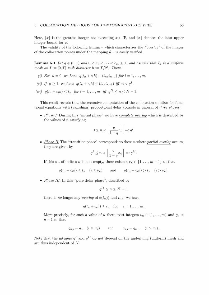
5 COLLOCATION METHODS FOR PANTOGRAPH-TYPE VFES 53
Here, bxc is the greatest integer not exceeding x ∈ IR, and dxe denotes the least upperinteger bound for x.
The validity of the following lemma – which characterizes the “overlap” of the imagesof the collocation points under the mapping θ – is easily verified.
Lemma 5.1 Let q ∈ (0, 1) and 0 < c1 < · · · < cm ≤ 1, and assume that Ih is a uniformmesh on I := [0, T ] with diameter h := T/N . Then:
(i) For n = 0 we have q(tn + cih) ∈ (tn, tn+1) for i = 1, . . . ,m.
(ii) If n ≥ 1 we have q(tn + cih) ∈ (tn, tn+1) iff n < qI .
(iii) q(tn + cih) ≤ tn for i = 1, . . . ,m iff qII ≤ n ≤ N − 1.
This result reveals that the recursive computation of the collocation solution for func-tional equations with (vanishing) proportional delay consists in general of three phases:
• Phase I: During this “initial phase” we have complete overlap which is described bythe values of n satisfying
0 ≤ n <
⌈q
1− qc1
⌉=: qI .
• Phase II: The “transition phase” corresponds to those n where partial overlap occurs;they are given by
qI ≤ n <
⌈q
1− qcm
⌉=: qII .
If this set of indices n is non-empty, there exists a νn ∈ {1, . . . ,m− 1} so that
q(tn + cih) ≤ tn (i ≤ νn) and q(tn + cih) > tn (i > νn).
• Phase III: In this “pure delay phase”, described by
qII ≤ n ≤ N − 1,
there is no longer any overlap of θ(tn,i) and tn,i: we have
q(tn + cih) ≤ tn for i = 1, . . . ,m.
More precisely, for such a value of n there exist integers νn ∈ {1, . . . ,m} and qn <n− 1 so that
qn,i = qn (i ≤ νn) and qn,i = qn+1 (i > νn).
Note that the integers qI and qII do not depend on the underlying (uniform) mesh andare thus independent of N .

5 COLLOCATION METHODS FOR PANTOGRAPH-TYPE VFES 54
Example 5.1:
We list a selection values of qI and qII for m = 2 and m = 3, corresponding to the
• Gauss points:
m = 2: c1 = (3−√
3)/6, c2 = (3 +√
3)/6,
m = 3: c1 = (5−√
15)/10, c2 = 1/2, c3 = (5 +√
15)/10;
• Radau II points:
m = 2: c1 = 1/3, c2 = 1,
m = 3: c1 = (4−√
6)/10, c2 = (4 +√
6)/10, c3 = 1.
Table 2: m = 2
Gauss points Radau II pointsq = 1/2 2/3 0.9 0.99 1/2 2/3 0.9 0.99qI = 1 1 2 21 1 1 3 33qII = 1 2 8 79 1 2 9 99
Table 3: m = 3
Gauss points Radau II pointsq = 1/2 2/3 0.9 0.99 1/2 2/3 0.9 0.99qI = 1 1 2 12 1 1 2 16qII = 1 2 8 88 1 2 9 99
Remark: Piecewise polynomial spaces based on geometric or quasi-geometric meshes willbe considered in Section 5.6.
5.3 Second-kind VFIEs with proportional delays
5.3.1 The structure of the cllocation equations
The collocation solution uh ∈ S(−1)m−1(Ih) for the delay integral equation (4.6) is defined by
uh(t) = g(t) + (Vuh)(t) + (Vθuh)(t), t ∈ Xh, (5.3)
with θ(t) = qt (0 < q < 1) and Xh given by (3.2) (hn = h). The contribution of the delayterm (Vθuh)(tn,i) to the collocation equation (5.3) will depend on n and the location ofthe collocation parameters {ci}: it follows from the definition of qn,i and γn,i in (5.1) that
(Vθuh)(tn,i) =∫ tqn,i
0K(tn,i, s)uh(s)ds + h
∫ γn,i
0K(tn,i, tqn,i + sh)uh(tqn,i + sh)ds. (5.4)

5 COLLOCATION METHODS FOR PANTOGRAPH-TYPE VFES 55
In order to obtain suitable computational forms of the collocation equation (5.3) (lead-ing to systems of difference equations whose solution describes the collocation solution onI), we again express uh on the subinterval σn by the local Lagrange representation,
uh(tn + vhn) =m∑
j=1
Lj(v)Un,j , v ∈ (0, 1] (0 ≤ n ≤ N − 1), (5.5)
with
Lj(v) :=m∏
k 6=j
(s− ck)/(cj − ck) and Un,j := uh(tn + cjhn),
and where we have assumed that hn = h = T/N for n = 0, 1, . . . , N − 1. The aboveexpression for (Vθuh)(tn,i) now becomes
(Vθuh)(tn,i) = h
qn,i−1∑`=0
m∑j=1
(∫ 1
0K(tn,i, t` + sh)Lj(s)ds
)U`,j
+hm∑
j=1
(∫ γn,i
0K(tn,i, tqn,i + sh)Lj(s)ds
)Uqn,i,j (5.6)
(i = 1, . . . ,m). Thus, the collocation equation (5.3) leads to a system of linear differenceequations for the vectors Un ∈ IRm (0 ≤ n ≤ N − 1) whose structure will change aswe pass from Phase I of complete overlap (0 ≤ n < qI) via Phase II of partial overlap(qI ≤ n < qII) to the pure delay Phase III (qIII ≤ n ≤ N −1). To make this more precise,we set gn := ( g(tn,1), . . . , g(tn,m) )T ∈ IRm and introduce the matrices
Bn :=
∫ ci
0K1(tn,i, tn + sh)Lj(s)ds
(i, j = 1, . . . ,m)
, (5.7)
Bn,` :=
∫ 1
0K1(tn,i, t` + sh)Lj(s)ds
(i, j = 1, . . . ,m)
(` < n). (5.8)
in L(IRm). These matrices correspond to the contribution to the difference equation dueto the “classical” (non-delay) Volterra operator V in (5.3). For the concise formulation ofthe terms in the difference equation describing Phases I, II, and III and corresponding tothe delay operator Vθ we introduce the following matrices in L(IRm) (the linear space ofreal square matrices of order m, in which Im denotes the identity matrix):
Phase I:
BIn(q) :=
∫ γn,i
0K2(tn,i, tn + sh)Lj(s)ds
(i, j = 1, . . . ,m)
, (5.9)
BIn,`(q) :=
∫ 1
0K2(tn,i, t` + sh)Lj(s)ds
(i, j = 1, . . . ,m)
(` < n). (5.10)
Here, Un (0 ≤ n < qI) is given by the solution of
[Im − h(Bn + BIn(q))]Un = gn + h
n−1∑`=0
(Bn,` + BIn,`(q))U`. (5.11)

5 COLLOCATION METHODS FOR PANTOGRAPH-TYPE VFES 56
Phase II:
BIIn (q) := diag( 0, . . . , 0︸ ︷︷ ︸
νn
, 1, . . . , 1 )BIn(q), (5.12)
BIIn−1(q) :=
∫ γn,i
0K2(tn,i, tn−1 + sh)Lj(s)ds
(i, j = 1, . . . ,m)
, (5.13)
SIIn−1(q) := diag( 0, . . . , 0︸ ︷︷ ︸
νn
, 1, . . . , 1 )BIn,n−1(q), (5.14)
SIIn−1(q) := diag( 1, . . . , 1︸ ︷︷ ︸
νn
, 0, . . . , 0 )BIIn−1(q). (5.15)
Here, diag ( d1, . . . , dm ) denotes a diagonal matrix in L(IRm) with diagonal elementsd1, . . . , dm. It is the readily verified that now Un (qI ≤ n < qII) is determined by thesolution of
[Im − h(Bn + BIIn (q))]Un = gn + h
n−1∑`=0
Bn,`U` + hn−2∑`=0
BIn,`(q)U`
+h[SIIn−1(q) + SII
n−1(q)]Un−1. (5.16)
Phase III:
BIIIqn
(q) :=
∫ γn,i
0K2(tn,i, tqn + sh)Lj(s)ds
(i, j = 1, . . . ,m)
, (5.17)
SIIIqn+1(q) := diag( 0, . . . , 0︸ ︷︷ ︸
νn
, 1, . . . , 1 )BIIIqn+1(q), (5.18)
SIIIqn
(q) := diag( 1, . . . , 1︸ ︷︷ ︸νn
, 0, . . . , 0 )BIIIqn
(q). (5.19)
Once we have reached this pure delay phase the vector Un (qII ≤ n ≤ N − 1) is given bythe solution of
[Im − hBn]Un = gn + hn−1∑`=0
Bn,`U` + hqn−1∑`=0
BIn,`(q)U` (5.20)
+h[SIIIqn
(q) + BIn,qn
(q)]Uqn + hSIIIqn+1(q)Uqn+1.
The (different) integers νn occurring in Phases II and III, and the integer qn < n − 1in Phase III were defined following Lemma 4.1.
Example 5.2: Suppose that the second-kind delay VIE (4.4) is solved by collocation inS
(−1)0 (Ih), with uniform mesh Ih and collocation points Xh = {tn + c1h : 0 < c1 ≤ 1 (0 ≤
n ≤ N−1)}. Since uh is constant on each subinterval σn we write yn+1 := uh(tn+vh) (v ∈(0, 1]).

5 COLLOCATION METHODS FOR PANTOGRAPH-TYPE VFES 57
For m = 1 we have qI = qII = dqc1/(1−q)e. Hence, the collocation equation (with V = 0)becomes(
1− h
∫ γn,1
0K(tn,1, tn + sh)ds
)yn+1 = h
n−1∑`=0
(∫ 1
0K(tn,1, t` + sh)ds
)y`+1 + g(tn,1)
when 0 ≤ n < qI . For qI ≤ n ≤ N − 1 it reads
yn+1 = g(tn,1) + h
qn,1−1∑`=0
(∫ 1
0K(tn,1, t` + sh)ds
)y`+1
+h
(∫ γn,1
0K(tn,1, tqn,1+1 + sh)ds
)yqn,1+1.
Thus, if K(t, s) ≡ b/q and g(t) ≡ 1 the collocation solution to the resulting DVIE
y(t) = 1 +∫ qt
0(b/q)y(s)ds, t ∈ I
(which is equivalent to the initial-value problem y′(t) = by(qt), y(0) = 1) is determinedby the solution of he difference equation
yn+1 = 1 +hb
q
qn,1−1∑`=0
y`+1 +hb
qγn,1yqn,1+1, (5.21)
where qn,1 := bqc1/(1− q)c and γn,1 := q(n + c1)− qn,1.We list, also for use in Example 5.2 in Section 5.3, a sample of values of qn,1 and γn,1
for c1 = 1/2, to provide some insight into the structure of the above difference equationswhen collocation is at the Gauss point tn + h/2.
Table 4: q = 1/2, c1 = 1/2 (qI = qII = 1)
n = 0 1 2 3 4 5 6qn,1 = 0 0 1 1 2 2 3γn,1 = 1/4 3/4 1/4 3/4 1/4 3/4 1/4
Table 5: q = 0.9, c1 = 1/2 (qI = qII = 5)
n = 0 1 2 3 4 5 6qn,1 = 0 1 2 3 4 4 5γn,1 = 0.45 0.35 0.25 0.15 0.05 0.95 0.85

5 COLLOCATION METHODS FOR PANTOGRAPH-TYPE VFES 58
For Volterra functional equations governed by the special delay operator Wθ (cf. (4.8))we find – in complete analogy to the above – that (Wθuh)(tn,i) is given by
(Wθuh)(tn,i) = h
∫ 1
γn,i
K(tn,i, tqn,i + sh)uh(tqn,i + sh)ds +∫ tn
tqn,i+1
K(tn,i, s)uh(s)ds
+h
∫ ci
0K(tn,i, tn + sh)uh(tn + sh)ds. (5.22)
This can be written as
(Wθuh)(tn,i) = hm∑
j=1
(∫ 1
γn,i
K(tn,i, tqn,i + sh)Lj(s)ds
)Uqn,i,j
+hn−1∑
`=qn,i+1
(∫ 1
0K(tn,i, t` + sh)Lj(s)ds
)U`,j (5.23)
+hm∑
j=1
(∫ ci
0K(tn,i, tn + sh)KLj(s)ds
)Un,j .
Hence, the collocation equation associated with y = g +Wθy,
uh(t) = g(t) + (Wθuh)(t), t ∈ Xh,
leads to the following systems of linear algebraic equations for Un ∈ IRm describing thelocal representation (5.5) of uh ∈ S
(−1)m−1(Ih) (again with uniform Ih):
Phase I:[Im − hBI
n(q)]Un = gn (0 ≤ n < qI), (5.24)
with
BIn(q) =
∫ ci
γn,i
K(tn,i, tn + sh)Lj(s)ds
(i, j = 1, . . . ,m)
,
which formally is equivalent to Bn + BIn(q) in (5.11) when K2 = −K1 =: −K;
Phase II:
[Im − hBIIn (q)]Un = gn + hSII
n−1(q)Un−1 (qI ≤ n < qII), (5.25)
where
BIIn (q) := diag( 1, . . . , 1︸ ︷︷ ︸
νn
, 0, . . . , 0 )Bn + diag( 0, . . . , 0︸ ︷︷ ︸νn
, 1, . . . , 1 )BIn(q),
and
SIIn−1(q) := diag( 1, . . . , 1︸ ︷︷ ︸
νn
, 0, . . . , 0 )
( ∫ 1
γn,i
K(tn,i, tn−1 + sh)Lj(s)ds
);
Phase III:
[Im − hBn]Un = gn + h[SIIIqn
(q)Uqn +n−1∑
`=qn+1
Bn,`U` + SIIIqn+1(q)Uqn+1], (5.26)

5 COLLOCATION METHODS FOR PANTOGRAPH-TYPE VFES 59
with
SIIIqn
(q) := diag( 1, . . . , 1︸ ︷︷ ︸νn
, 0, . . . , 0 )
( ∫ 1
γn,i
K(tn,i, tqn + sh)Lj(s)ds
),
SIIIqn+1(q) := diag( 1, . . . , 1︸ ︷︷ ︸
νn
, 0, . . . , 0 )Bn,qn+1 +
+diag( 0, . . . , 0︸ ︷︷ ︸νn
, 1, . . . , 1 )
( ∫ 1
γn,i
K(tn,i, tqn+1 + sh)Lj(s)ds
).
The matrices Bn,` ∈ L(IRm) coincide with the ones in (5.8).
5.3.2 Optimal orders of convergence
Suppose that a given delay integral with (vanishing) proportional delay is solved by col-location in S
(−1)m−1(Ih), with the underlying mesh Ih being a uniform one, and assume that
the functions defining the functional equation have arbitrarily high degree of regularityon their respective domains (implying, as we have seen in Theorem 4.4, that the exactsolution has the same regularity). What can be said, as h → 0, N →∞ (Nh = T ) aboutthe optimal values of p and p∗ in the estimates
||y − uh||∞ := sup{|y(t)− uh(t)| : t ∈ I} ≤ C(q)hp (5.27)
and||y − uh||Ih,∞ := max{|y(t)− uh(t)| : t ∈ Ih \ {0}} ≤ C(q)hp∗ ? (5.28)
Do higher values of p and p∗ result for the iterated collocation solution uith based on uh?
It turns out that we have p = m in the global estimate (5.27) if the set {ci} is arbi-trary; that is, the results that hold for “classical” VIEs of the second kind remain valid.However, the question regarding the optimal value of p∗ in (5.28) (attainable order oflocal superconvergence on Ih \ {0}) has an answer that differs sharply from the one fornon-delay VIEs. Moreover, we shall see that it is not yet known under what conditionson the collocation parameters {ci} the collocation solutions uh to the first-kind delay VIE(4.27) converge uniformly on I to the exact solution y (see also Section 5.3).
Theorem 5.2 Consider the second-kind VFIE (4.6) and assume that the given functionsg, K1, K2 are at least m times continuously differentiable on their respective domains.Then, for all sufficiently small h > 0 (so that the difference equations (5.11), (5.16), (5.20)possess unique solutions), we have p = m in (5.27) for arbitrary {ci} in Xh and for alldelay functions θ(t) = qt with 0 < q < 1. The constant C(q) depends on the {ci} and onq but not on h.
The proof of this result is an adaptation of the one for classical second-kind VIEs andVFIEs with non-vanishing delays: it consists in showing that in each of the Phases I –III the `1-norms of the vectors Un defined by (5.11), (5.16), and (5.20) satisfy a discreteGronwall inequality. An elementary induction argument then leads to the assertion, ob-serving the local representation (5.5) of uh and the fact that, by the assumption on the
5 COLLOCATION METHODS FOR PANTOGRAPH-TYPE VFES 60
regularity of the given data, y ∈ Cm(I). The detailed arguments can be found in Chapter5 (Section 5.3) of Brunner (2004a); see also Zhang (1998) and Brunner & Zhang (1998)for related results.
We now turn to the question of global and local superconvergence on I and Ih, respec-tively: are there collocation parameters {ci} for which p = m in (5.27) can be replacedby p∗ > m, and how large can p∗ become in (5.28? Assume that the solution of thesecond-kind VFIE (4.6) is approximated by the collocation solution uh ∈ S
(−1)m−1(Ih) and
the corresponding iterated collocation solution,
uith (t) := g(t) + (Vuh)(t) + (Vθuh)(t), t ∈ I. (5.29)
Recall that uith (t) = uh(t) whenever t ∈ Xh; in particular, if cm = 1 then tn ∈ Xh and
hence uith (tn) = uh(tn) (n = 1, . . . , N).
It is well known (see, e.g., Brunner & van der Houwen (1986) (Chapter 5)) that ifVθ = 0 (classical Volterra integral equation) and if the {ci} are the Gauss (-Legendre)points (given by the zeros of the shifted Legendre polynomial Pm(2s − 1)), then we onlyattain p∗ = m in (5.28): local superconvergence of order p∗ = 2m is only possible if uh
is replaced by the iterated collocation solution uith . For the general delay VIE (4.6) with
θ(t) = qt (0 < q < 1) this is no longer true (see Brunner (1997), Takama et al. (2000),Muroya et al. (2003), Brunner (2004b)): for arbitrary q ∈ (0, 1) we have p∗ < 2m whenm ≥ 3. The results of Theorems 5.3 and 5.5 have recently been established in Brunner &Hu (2005). Theorem 5.5 disproves a conjecture in Brunner (1997a) and Brunner, Hu &Lin (2001) for m > 2.
Theorem 5.3 Let the collocation parameters {ci} satisfy the orthogonality condition
J0 :=∫ 1
0
m∏i=1
(s− ci) ds = 0. (5.30)
Then||y − uit
h ||∞ ≤ C(q)hm+1,
where uith is the iterated collocation approximation (5.29) corresponding to the collocation
solution uh ∈ S(−1)m−1(Ih) for (4.4). Here, m + 1 cannot, in general, be replaced by m + 2
We note that the most prominent set of parameters {ci} satifying the above orthogo-nality condition are the Gauss points.
Proof: We will sketch the principal steps leading to the above global superconvergenceresult by using an approach different from the one in Brunner & Hu (2005). For ease ofnotation we will do this for (4.4) with V = 0,
y(t) = g(t) + (Vθy)(t), t ∈ I.
In this case, the collocation error eh := y − uh satisfies the integral equation
eh(t) = δh(t) + (Vθeh)(t), t ∈ I, (5.31)

5 COLLOCATION METHODS FOR PANTOGRAPH-TYPE VFES 61
where the defect δh vanishes on Xh and inherits (piecewise, on each subinterval σn) theregularity of g and K2. Moreover, we have eit
h := y− uith = eh − δh. Hence, it follows from
the solution representation (4.5) in Theorem 4.2 that
eith (t) =
∞∑j=1
∫ qjt
0K2,j(t, s)δh(s)ds, t ∈ I. (5.32)
Here, K2,j(t, s) denotes the jth iterated kernel of the given kernel K2(t, s) in Vθ (cf.Theorem 4.2)), and the infinite series converges uniformly on I.
Let now t = tn + vh, v ∈ [0, 1] be given and define, as in (5.1),
qj,n(v) := bqj(n + v)c, γj,n(v) := qj(n + v)− qj,n(v) ∈ [0, 1) (j ∈ IN).
This allows us to write (5.32) in the form
eith (t) =
∞∑j=1
(∫ tqj,n (v)
0K2,j(t, s)δh(s)ds
+h
∫ γj,n(v)
0K2,j(t, tqj,n(v) + sh)δh(tqj,n(v) + sh)ds
). (5.33)
The assertion in Theorem 5.3 now follows from the following observations:
(i) Since 0 < q < 1, we have qj,n(v) < N for all n ≤ N − 1 and v ∈ [0, 1]. Upon writing
∫ tqj,n (v)
0K2,j(t, s)δh(s)ds = h
qj,n(v)−1∑`=0
∫ 1
0K2,j(t, t` + sh)δh(t` + sh)ds,
we can again resort to the classical “quadrature error argument”i of Sections 3.4.2and 3.4.3, consisting in replacing each of the above integrals by the sum of the inter-polatory m-point quadrature approximation based on the points {t` + cih} and thecorresponding quadrature error. As δh(t` + cih) = 0, and Nh = T , it follows thatthe absolute values of the integrals are bounded by CQhm+1, because the orthogo-nality condition (5.30) implies that the quadrature formulas all possess a degree ofprecision of (at least) m.
(ii) The global convergence estimate given by Theorem 5.2 can be used in (5.31) toobtain the estimate
||δh||∞ ≤ (1 + ||Vθ||)C(q)hm,
where
||Vθ|| := maxt∈Dθ
∫ θ(t)
0|K2(t, s)|ds.
(iii) The iterated kernels K2,j(t, s) satisfy
|K2,j(t, s)| ≤qj(j−1)/2
(j − 1)!T j−1Kj
θ , t ∈ D(j)θ

5 COLLOCATION METHODS FOR PANTOGRAPH-TYPE VFES 62
(cf. Lemma 4.3)), where
Kθ := max(Dθ)
|K2(t, s)| and D(j)θ := {(t, s) : 0 ≤ s ≤ qjt, t ∈ I}.
This result implies that the infinite series involving the second terms on the right-hand side of (5.33) converges uniformly and is O(hm+1).
In contrast to this result (the analogue of the global superconvergence result for ODEs),collocation at the Gauss points does no longer lead to local superconvergence of order 2mon Ih when m ≥ 3, as the following theorem shows. (Observe that for m = 2 we have2m = m + 2.) A first hint that this is so may be devined from the following resultcomparing the collocation solution for the special pantograph equation (4.2) with theiterated collocation solution (based on the same collocation parameters) for its integratedform,
y(t) = y0 +∫ qt
0(b/q)y(s)ds, t ∈ I.
Theorem 5.4 Assume:
(a) uh ∈ S(−1)m−1(Ih) is the collocation solution (with respect to Xh) to the integrated
form of y′(t) = by(qt), y(0) = y0 (b 6= 0, y0 6= 0), and uith denotes the corresponding
iterated collocation solution.
(ii) vh ∈ S(0)m (Ih) is the collocation solution (also with respect to Xh) to y′(t) =
by(qt), y(0) = y0.
Then we have, for all q ∈ (0, 1),
uith (t) 6= vh(t) whenever t ∈ Ih \ {0}.
Remark: We remind the reader that for q = 1 we obtain uith (t) = vh(t) for all t ∈ I: the
“indirect” collocation approximation uith has the same (super-) convergence properties as
the “direct” one for the original ODE.
The proof of the following theorem is based on interpolatory projection techniques andcan be found in Brunner & Hu (2005).
Theorem 5.5 Assume that g, K1 and K2 in (4.6) possess continuous derivatives of ar-bitrary orders on their respective domains. Let uh ∈ S
(−1)m−1(Ih) be the collocation solution
corresponding to the Gauss points {ci}, and let the iterated collocation solution be definedby (5.29). Then for any q ∈ (0, 1) and m ≥ 1, the order p∗ in the local estimate
||y(t)− uith (t)||h,∞ ≤ C(q)hp∗
cannot exceed m + 2, regardless of the value of d. More precisely, the following is true:

5 COLLOCATION METHODS FOR PANTOGRAPH-TYPE VFES 63
(i) If q = 1/2 then
||y − uith ||h,∞ ≤ C(q)
{hm+2 if m is even,hm+1 if m is odd.
(ii) For q ∈ (0, 1) \ {1/2}, we have
||y − uith ||h,∞ ≤ C(q)hm+1,
for all m ≥ 2.
Remarks:
1. Numerical evidence shows that the error constants C(q) in the above order estimatesappear to depend strongly on q as q → 1− (see also the paper by Elbert (1992)).Thus, it is a challenging problem to find this dependence on q explicitly: even insightobtained from a simple (linear) “toy problem” like (4.2) would be valuable.
2. For the more general second-kind VFIE (4.9), which we write now as
y(t) = g(t) + b(t)y(θ(t)) + (Wθy)(t), t ∈ I (θ(t) = qt, 0 < q < 1),
the existence of a unique collocation solution uh ∈ S(−1)m−1(Ih) is no longer guaranteed
in Phases I and II for all sufficiently small mesh diameters h > 0. This is due to thepresence of the terms b(tn,i)uh(θ(tn,i)) which, using the local representation of uh onσqn,i (cf. (5.5)), assume the form b(tn,i)
∑mj=1 Lj(γn,i)Uqn,i,j (i = 1, . . . ,m). Thus,
the matrix describing the left-hand side of the difference equation (5.11) (Phase I)is now Im − Bn − h(Bn + BI
n(q)), with
Bn := diag( b(tn,i) )
(Lj(γn,i)
(i, j = 1, . . . ,m)
),
and hence its inverse will no longer exist for all sufficiently small h > 0. (Comparealso Liu (1995b) where this problem is studied for the case Wθ = 0, m = 1, andc1 = 1.) The superconvergence analysis for this more general Volterra integralequation with proportional delay is yet to be established.
5.4 First-kind VFIEs with proportional delays
Turning to Volterra’s first-kind VFIE with proportional delay θ(t) = qt (0 < q < 1) of1897,
(Wθy)(t) = g(t), t ∈ I := [0, T ], (5.34)
the linear algebraic systems whose solutions Un ∈ IRm define the local representations(5.5) of its collocation solution uh ∈ S
(−1)m−1(Ih) can be obtained from (5.24)–(5.26): they
are, respectively,BI
n(q)Un = h−1gn (0 ≤ n < qI), (5.35)

5 COLLOCATION METHODS FOR PANTOGRAPH-TYPE VFES 64
BIIn (q)Un = h−1gn − SII
n−1(q)Un−1 (qI ≤ n < qII), (5.36)
and
BnUn = h−1gn − [SIIIqn
(q)Uqn +n−1∑
`=qn+1
Bn,`U` + SIIIqn+1(q)Uqn+1 (qII ≤ n ≤ N − 1),
(5.37)respectively.
Example 5.3: Consider the first-kind VFIE (5.34), and assume that its collocation solu-tion is to be in the collocation space of Example 5.1. Thus, for 0 ≤ n < qI the collocationequation at t = tn,1 = tn + c1h may be written in the form(∫ c1
γn,1
K(tn,1, tn + sh)ds
)yn+1 = h−1g(tn,1).
If n ≥ qI = qII (see Example 5.1) we have, by (5.22),
(Wθuh)(tn,1) =∫ tn
qtn,1
K(tn,1, s)uh(s)ds +∫ tn,1
tnK(tn,1, s)uh(s)ds,
and this can be written as(∫ c1
0K(tn,1, tn + sh)ds
)yn+1 = h−1g(tn,1)−
(∫ 1
γn,1
K(tn,1, tqn,1 + sh)ds
)yqn,1+1
−n−1∑
`=qn,1+1
(∫ 1
0K(tn,1, t` + sh)ds
)y`+1.
Setting
An :=∫ c1
0K(tn,1, tn + sh)ds, Bn,` :=
∫ 1
0K(tn,1, t` + sh)ds (qn,1 + 1 ≤ ` ≤ n− 1),
and
Cn,qn :=∫ 1
γn,1
K(tn,1, tqn,1 + sh)ds,
with qn,1 := bq(n + c1)c and γn,1 := q(n + c1) − qn,1, the above difference equation for{yn+1} becomes
Anyn+1 +n−1∑
`=qn,1+1
Bn,`y`+1 + Cn,qnyqn,1+1 = h−1g(tn,1). (5.38)
If K(t, s) ≡ 1, the delay integral equation (5.34) reduces to∫ t
qty(s)ds = g(t), t ∈ I (g(0) = 0),
and this is equivalent to the functional equation
y(t)− qy(qt) = g′(t), t ∈ I.

5 COLLOCATION METHODS FOR PANTOGRAPH-TYPE VFES 65
The corresponding collocation solution uh ∈ S(−1)0 (Ih) is thus determined by the solution
of the difference equation
c1yn+1 +n−1∑
`=qn,1+1
y`+1 + (1− γn,1)yqn,1+1 = h−1g(tn + c1h) (n ≥ 0). (5.39)
In order to obtain the difference equation corresponding to collocation at the Gauss points(c1 = 1/2) recall Tables 2 and 3 of Example 5.1 (Section 5.2.1) for the values of qn,1 andγn,1.
What can be said about the attainable orders of global and local (super-) convergence:how do the analogues of Theorems 5.2, 5.3 and 5.4 look like? As we have briefly mentionedbefore, the analysis leading to answers for these questions remains open. We only knowfrom numerical evidence that the condition
−1 ≤ ρm := (−1)mm∏
i=1
1− ci
ci≤ 1
(which guarantees uniform convergence when q = 0 in Wθ with θ(t) = qt) is no longersufficient for this to be true. In particular, it is not yet known for which values of c1 ∈(0, 1] the solution of the simple difference equation (5.38) remains uniformly bounded asN →∞ (h → 0, Nh = T ) when q ∈ (0, 1).
5.5 VFIDEs with proportional delays
The collocation solution uh ∈ S(0)m (Ih) for the VFIDE (4.12) is determined by
u′h(t) = a(t)uh(t) + b(t)uh(θ(t)) + (Wθuh)(t), t ∈ Xh, (5.40)
with initial condition uh(0) = y0. Since the collocation space is now a subspace of C(I)the system of difference equations arising in the computation of uh has a somewhat morecomplex structure than the ones we encountered in the previous section. To be somewhatmore precise, the local representation of uh ∈ S
(0)m (Ih) is now
uh(tn + vh) = yn + hm∑
j=1
βj(v)Yn,j , v ∈ [0, 1] (0 ≤ n ≤ N − 1), (5.41)
where yn := uh(tn), Yn,j := u′h(tn,j), and βj(v) :=∫ 10 Lj(s)ds. Hence, the key ingredients
in the derivation of the difference equations are essentially the same as in Section 5.2, thatis, the terms of (Wθuh)(tn,i) corresponding to Phases I, II, and III and containing thevectors Yn are described by matrices similar to those in (5.24)–(5.26), except that insteadof Lj(s) their integrands contain the integrated Lagrange polynomials βj(s). However,there are now also additinal terms reflecting the continuity constraint of uh at the interiormesh points t1, . . . , tN−1. We leave the details to the reader; compare also Chapter 5 inBrunner (2004a). Instead, we present an illustration from which the difference equationsfor arbitrary m ≥ 2 can readily be deduced.

5 COLLOCATION METHODS FOR PANTOGRAPH-TYPE VFES 66
Example 5.4: Consider (5.40) and suppose that uh ∈ S(0)1 (Ih) (m = 1), with 0 < c1 ≤ 1.
The collocation equation defining this collocation solution uh,
u′h(tn,1) = a(tn,1)uh(tn,1) + b(tn,1)uh(qtn,1) + (Wθuh)(tn,1),
where, by (5.41), uh(tn + vh) = yn + hvYn,1 (v ∈ [0, 1]), can be written as
Yn,1 = a(tn,1){yn + hc1Yn,1}+ b(tn,1){yqn,1 + hγn,1Yqn,1}+ (Wθuh)(tn,1),
with
(Wθuh)(tn,1) =∫ tqn,1+1
tqn,1
K(tn,1, s)uh(s)ds +∫ tn
tqn,1+1
K(tn,1, s)uh(s)ds
+h
∫ c1
0K(tn,1, tn + sh){yn + hsYn,1}ds.
Hence, the resulting difference equation is(1− ha(tn,1)c1 − h2
∫ c1
0K(tn,1, tn + sh)s ds
)Yn,1
= [hb(tn,1)γn,1 + h2
(∫ 1
γn,1
K(tn,1, tqn,1 + sh)s ds
)]Yqn,1 (5.42)
+h2n−1∑
`=qn,1+1
(∫ 1
0K(tn,1, t` + sh)s ds
)Y`,1 + ρn,
where
ρn := a(tn,1)yn +
(b(tn,1) + h
∫ 1
γn,1
K(tn,1, tqn,1 + sh)ds
)yqn,1
+hn−1∑
`=qn,1+1
(∫ 1
0K(tn,1, t` + sh)ds
)y` + h
(∫ c1
0K(tn,1, tn + sh)ds
)yn.
The values of qn,1 and γn,1 can be found in Example 5.1. Observe also that the abovedifference equation (5.42) can be reformulated as a difference equation for {yn}, by settingYn,1 = (yn+1 − yn)/h (cf. (5.41) with m = 1 and v = 1).
Remark: The problem of asymptotic stability for uh in special case corresponding toW = 0 and constant coefficients a, b, i.e. the pantograph equation (4.1), was studied inBuhmann, Iserles & Nørsett (1993) and Iserles (1994a) for q = 1/2. For other values of q,and for pantograph-type VFIDEs, the problem remains open (see also Section 6.5).
5.5.1 Optimal convergence estimates
The first theorem shows that the classical global order of convergence remains also validfor VFIDEs with vanishing proportional delay. The proof is again based on a “PhaseI – III” Gronwall-type inductive argument; the details can be found in Brunner (2004)(Section 5.5). See also Zhang (1998) and Brunner & Zhang (1998) for some related results.

5 COLLOCATION METHODS FOR PANTOGRAPH-TYPE VFES 67
Theorem 5.6 Consider the VFIDE (4.12) (which includes (4.14) and the pantographequation (4.1) as special cases) and assume that the given functions a, b, K1 and K2
are at least m times continuously differentiable on their respective domains. Then for anyθ(t) = qt with q ∈ (0, 1) and for all sufficiently small h > 0 the unique collocation solutionuh ∈ S
(0)m (Ih) given by (5.40) satisfies
||yν) − u(ν)h ||∞ := sup{|y(ν)(t)− u
(ν)h (t)| : t ∈ I} ≤ Cν(q)hm (ν = 0, 1),
and this holds for any set {ci} defining the collocation points Xh. The constants Cν(q)depend on the {ci} and on q but not on h.
As for VFIEs of the second kind with proportional delays, local superconvergence resultsfor analogous VFIDEs differ sharply from the classical results. However, the global orderp = m + 1 is possible for the collocation solution uh ∈ S
(0)m (Ih). We summarise this
results, and a conjecture, below. Note, incidentally, that these delay VIDEs include thepantograph equation and its counterpart with variable coefficients a and b as special cases.
Theorem 5.7 Let uh ∈ S(0)m (Ih) be the collocation solution to the proportional delay
VFIDE (4.12). If the given functions possess continuous derivatives of at least order m+1on their respective domains, and if the {ci} satisfy the orthogonality condition (5.30) ofTheorem 5.3, then
||y − uh||∞ ≤ C(q)hm+1
holds for all q ∈ (0, 1).
Proof: We write the error equation for (5.40),
e′h(t) = a(t)eh(t) + b(t)eh(qt) + δh(t) + (Veh)(t) + (Vθeh)(t), t ∈ I, eh(0) = 0,
in integrated form. The analysis in Brunner & Hu (2005) (or, if a(t) ≡ 0, V = 0, theone employed in the proof of Theorem 5.3) can then be applied to the resulting delayintegral equation for eh. The detailed proof can be found in Brunner & Hu (2007); seealso Brunner (2008a).
Finally, we turn to the question of the optimal order of local superconvergence onuniform meshes. As the following theorem reveals (see Brunner and Hu (2007)), thisorder cannot exceed m + 2 when m ≥ 2. This is similar to the result of Theorem 5.5 forVFIEs but, in contrast, is now rue for all q ∈ (0, 1).
Theorem 5.8 Suppose that uh ∈ S(0)m (Ih) is the collocation solution to the initial-value
problem for the VFIDE (5.40), where the underlying mesh is uniform and collocation iswith respect to the m Gauss points {ci} in (2.2). For all sufficiently smooth data and forany pantograph-type delay function θ(t) = qt with 0 < q < 1, the resulting collocation errorsatisfies
max1≤n≤N
|y(tn)− uh(tn)| ≤ C(q)hp∗ ,

5 COLLOCATION METHODS FOR PANTOGRAPH-TYPE VFES 68
with
p∗ =
{2m if m = 1, 2,m + 2 if m ≥ 3,
and where the constant C(q) does not depend on h. The above orders p∗ are best possiblefor nontrivial solutions.
Question: Can the local superconvergence reults of Theorems 5.8 and 5.5 be establishedby employing the embedding techniques described in Section 4.5 ?
Remark: The extension of the superconvergence analysis of collocation solutions inS
(0)m (Ih), with uniform mesh Ih, for neutral (linear and nonlineari) VFIDEs, in partic-
ular for VFIDEs of of Hammerstein type,
y′(t) = f(y(t), y(qt), y′(qt)) +∫ t
qtk(t− s)G(y(s), y′(s))ds (0 < q < 1),
remains to be established. (The theory of nonlinear pantograph-type DDEs, in particularwith nonlinearities of (Riccati or rational) forms, is considered in Iserles (1994b).)
5.6 Collocation using geometric meshes
The special form of the delay function θ(t) = qt (0 < q < 1) suggests that uith might
possibly attain the classical optimal order of superconvergence p∗ = 2m on Ih if Ih is asuitable geometric mesh and if collocation is at the Gauss points. That this is (almost) sowas verified in the paper by Brunner, Hu and Lin (2001). We briefly describe this resultand sketch its proof.
Assume that Ih is a geometric mesh defined by
Ih := {tn : tn = γN−nT, n = 0, 1, . . . , N ; γ ∈ (0, 1)}. (5.43)
The mesh parameter γ will depend, as is made precise below, on N (but not on n), on q,and on m. This mesh possesses the following obvious properties:
(i) hn := tn+1 − tn = γN−n−1(1− γ)T (n = 0, 1, . . . , N − 1);
(ii) max(n) hn = hN−1 = (1− γ)T (for any N ∈ IN). Hence, γ = γ(N) will have to bechosen so that γ → 1−, as N →∞, for all q ∈ (0, 1).
Let ρ ∈ IN be defined by
ρ :=
ln(q)
ln(1− 2m ln(N)(m+1)N )
: (5.44)
it is the largest integer for which
q1/ρ ≤ 1− 2m · ln(N)(m + 1)N
.

5 COLLOCATION METHODS FOR PANTOGRAPH-TYPE VFES 69
Theorem 5.9 will reveal the motivation for introducing this integer ρ. Observe that forgiven (fixed) q ∈ (0, 1) and m ≥ 1, we have ρ > 1 for all sufficiently large N . This is truebecause
1− 2m · ln(N)(m + 1)N
−→ 1−, as N →∞,
for any m ∈ IN.
Theorem 5.9 Assume:
(a) g ∈ C2m(I), K1 ∈ C2m(D), K2 ∈ C2m(Dθ);
(b) Ih is the geometric mesh described by (5.43) and (5.44), with γ = q1/ρ;
(c) uh ∈ S(−1)m−1(Ih) is the collocation solution to the delay VIE (4.6), with the {ci}
given by the Gauss points, and uith denotes the corresponding iterated collocation
solution.
Then for all sufficiently large N the resulting local order of convergence of uith is given by
maxt∈Ih\{0}
|y(t)− uith (t)| ≤ C(q)N−(2m−εN ),
where
εN := logN
((2m · ln(N))2m
(2m + 1)(m + 1)2m
)satisfies
limN→∞
εN = 0.
Proof: Since the proof is technically quite complex (using interpolatory projection tech-niques), we will only exhibit one of its key ingredients, namely
Lemma 5.10 Let Ih be the geometric mesh (5.43), (5.44), with γ = q1/ρ. Then:
(i) h0 ≤ CN−2m/(m+1);
(ii)N−1∑n=1
h2m+1n ≤ CN−(2m−εN );
(iii) For ρ + 1 ≤ n ≤ N we have qtn = tn−ρ ∈ Ih \ {0}.
Note, incidentally, that proposition (iii) may be viewed as generalised θ-invariance for thisgeometric mesh Ih.
Remarks:
1. Geometric meshes similar to the ones employed here were introduced by Hu (1998) forpiecewise polynomial collocation methods applied to VIDEs with weakly singularkernels, to obtain local superconvergence of the collocation solution on Ih.

5 COLLOCATION METHODS FOR PANTOGRAPH-TYPE VFES 70
2. Analogous superconvergence results can be derived for collocation solutions in S(0)m (Ih),
with suitable geometric meshes Ih, for the VFIDE (4.12) with proportional delays.The detailed analysis can be found in Brunner and Hu (2007).
3. Collocation (and Runge-Kutta) methods using quasi-geometric meshes are studied inBellen (2002) (for pantograph-type DDEs) and in Bellen, Brunner, Maset & Torelli(2006) (for pantograph-type VFIDEs). Assuming that a high-order approximationto the solution y has been found on some suitably “small” initial interval [0, t0](where t0 = t0(q, N)), one defines a geometric macro-mesh by the points ξµ :=q−µt0 (µ = 0, . . . ,M + 1), with appropriate M ≥ 1; on each interval [ξµ, ξµ+1] a(usually uniform) local mesh is introduced (similar to (3.3)). This “non-vanishingdelay approach” allows to obtain collocation (and Runge-Kutta) solutions of theclassical high orders. Details can be found in the above-mentioned papers.
5.7 Equations with nonlinear vanishing delays
In the foregoing analysis we have assumed that the delay function θ is given by thepantograph-type (linear) function θ(t) = qt (0 < q < 1). Assume now that θ is nonlinearand satisfies the following conditions:
(N1) θ(0) = 0, and θ is strictly increasing on I := [0, T ];
(N2) θ(t) ≤ q1t on I for some q1 ∈ (0, 1);
(N3) θ ∈ Cd(I) for some d ≥ 1.
It is then not difficult to verify that the solution representations for the VFIE (4.4) andthe VFIDE (4.12), with θ(t) replacing qt, have the same forms: the limits of integrationqnt and q−nt become
θn(t) := (θ ◦ · · · ◦ θ)︸ ︷︷ ︸n times
(t) and θ−n(t) =: (θ−1 ◦ · · · ◦ θ−1)︸ ︷︷ ︸n times
(t),
respectively. Details can be found in Brunner & Hu (2007), Brunner 2008a), Brunner(2008b).
5.8 VFEs with multiple vanishing delays
Let θj(t) := qjt be given delay functions with 0 < q1 < · · · < qr < 1 (r ≥ 2) andt ∈ I := [0, T ], and denote by Vθj
: C(I) → C(I) the linear Volterra integral operatorcorresponding to θj ,
(Vθjy)(t) :=
∫ θj(t)
0Kj(t, s)y(s) ds (j = 1, . . . , r). (5.45)
Consider the multi-delay the Volterra functional integro-differential equation
y′(t) = a(t)y(t) +r∑
j=1
bj(t)y(θj(t)) + g(t) +r∑
j=1
(Vθjy)(t), t ∈ I, (5.46)

5 COLLOCATION METHODS FOR PANTOGRAPH-TYPE VFES 71
with initial condition y(0) = y0, and the analogous multi-delay Volterra functional integralequation
y(t) = g(t) +r∑
j=1
(Vθjy)(t), t ∈ I, (5.47)
The former contains as an important special case the ‘multi-pantograph equation’,
y′(t) = au(t) +r∑
j=1
bjy(qjt) (5.48)
(see, e.g., Derfel (1990, 1991), Iserles & Liu (1994), Qiu, Mitsui & Kuang (1999), Ishi-wata (2000), Liu and Li (2004), and Zhao, Xu & Qiao (2005). Note that, in analogyto pantograph-type VFEs, multi-delay pantograph-type VFIDEs and VFIEs with smoothdata have solutions that are globally smooth on the given interval I.
Suppose that the multi-pantograph VFIDE (5.46) is solved by collocation in S(0)m (Ih),
using uniform Ih and collocation points
Xh := {tn + cih : 0 < c1 < · · · < cm ≤ 1 (0 ≤ n ≤ N − 1)}.
It turns out that if the {ci} are the Gauss points, then the optimal global and localsuperconvergence estimates of Theorems 5.7 and 5.8 remain valid. In contrast, the iteratedcollocation solution corresponding to the collocation solution uh ∈ S
(−1)m−1(Ih) for the multi-
pantograpg VFIE ( 5.47) does no longer exhibit local superconvergence of order m+2 (cf.Theorem 5.5). Details can be found in Brunner (2008d).
6 ADDITIONAL TOPICS AND CONCLUDING REMARKS 72
6 Additional topics and concluding remarks
Due to limitation of space (and time!) there are a number of aspects of VFEs we cannotconsider in detail in these notes and in the four lectures. The following sections contain abrief guide to some of these topics.
6.1 VFIEs and VFIDEs with weakly singular kernels
We start by briefly touching upon the the convergence properties of collocation solutionsto VFIEs and VFIDEs of the forms
y(t) = g(t) + (Vαy)(t) + (Vθ,αy)(t), (6.1)
andy′(t) = a(t)y(t) + b(t)y(θ(t)) + (Vθy)(t) + (Vθ,αy)(t), (6.2)
respectively. Here, the Volterra integral operators correspond to kernels containing a weak(i.e. unbounded but integrable) singularity:
(Vαy)(t) :=∫ t
t0(t− s)−αK1(t, s)y(s)ds, (Vθ,αy)(t) :=
∫ θ(t)
t0(t− s)−αK2(t, s)y(s)ds,
with 0 < α < 1 and smooth Ki (i = 1, 2). For non-vanishing delay functions θ theregularity of solutions for (6.1) and (6.2), as well as for the related neutral VFIDE
d
dt[y(t)− (Vθ,αy)(t)] = F (t, y(t), y(θ(t)), y′(θ(t))), (6.3)
is analysed in Brunner & Ma (2006) in the case of non-vanishing delay functions sθ.(Compare also the paper by Ito & Turi (1991) for VFIDEs of the form (6.3).)
For smooth data the solutions of (6.1) and (6.2) are not smooth at t = t0: in analogyto classical (non-delay) VIEs and VIDEs with weakly singular kernels (Brunner, Pedas &Vainikko (1999, 2001)), they behave like
|y′(t)| ≤ C(t− t0)−α and |y′′(t)| ≤ C(t− t0)−α (t0 < t ≤ T ),
respectively. This singular behaviour implies that on uniform meshes the collocationsolutions will not exhibit the optimal orders of Theorems 3.3, 3.4 and 3.10, 3.11 (seeBrunner (2004a, 2006)).
For VFIEs and VFIDEs with non-vanishing delays, one way of restoring the high order
of convergence in collocation solutions is to choose the mesh Ih =M⋃
µ=0
I(µ)h (recall (3.3))
where the local meshes I(µ)h are now graded:
I(µ)h := {t(µ)
n := ξµ +(
n
N
)rµ
(ξµ+1 − ξµ) : n = 0, 1, . . . , N}, (6.4)
with (local) grading exponents rµ > 1 depending on α and µ. Note that we have ξµ+1−ξµ =τ(ξµ+1) ≥ τ0 > 0.
6 ADDITIONAL TOPICS AND CONCLUDING REMARKS 73
Theorem 6.1 Let Ih be a θ-invariant mesh defined by (3.3) and (3.4), and assume thatthe first local mesh I
(0)h is graded with grading exponent r0 = r0(α) > 1; that is,
I(0)h := {t(0)n =
(n
N
)r0
(ξ1 − t0) : n = 0, 1, . . . , N}.
(i) If the lag function θ is linear, then the initial grading is inherited by the macro-meshes I
(1)h , . . . , I
(M)h , with rµ = r0 for all µ.
(ii) If θ is nonlinear, the grading is lost for I(µ)h (µ ≥ 1): these local meshes are no longer
graded ones of the form (6.4).
This result tells us that for the weakly singular VFIEs and VFIDES (6.1) and (6.2)with non-vanishing delays, collocation on θ-invariant meshes Ih with optimally gradedinitial mesh I
(0)h will exhibit the classical optimal global and local convergence orders if
the delay function θ is linear. For nonlinear θ, this will no longer be true. The readermay find details of the underlying analysis in Brunner (2004a) (Section 8.5.1) and Brunner(2006).
If the delay function θ in (6.1) or (6.2) vanishes at t = t0 (for example, is θ(t) = qt (0 <q < 1) with t0 = 0), then solutions corresponding to smooth data again are non-smoothat t = t0, as in (6.4), but are smooth on (t0, T ] (Brunner (2008c)). The convergenceanalysis of collocation (and discontinuous Galerkin) solutions on suitably graded meshesis currently being studied by the author and D. Schotzau.
6.2 VFIEs and VFIDEs with advanced arguments
The theory and the numerical analysis of VFEs with delay function satisfying θ(0) = 0and θ(t) > t for t > 0 remain to be studied. This is in particular true for pantographequation,
y′(t) = ay(t) + by(qt), t ≥ 0 :
if q > 1, then the corresponding initial-value problem is ill-posed. A detailed analysis ofsuch advanced differential equations can be found in Kato & McLeod (1971) (Theorem 2)and in Kato (1972). This ill-posedness will cause difficulties in the numerical solution ofsuch functional differential equations; a simple illustration of is given in Iserles (1994a) (pp.137-138) for the trapezoidal method. The general numerical analysis of, e.g., piecewisepolynomial collocation methods for pantograph-type DDEs and more general VFEs withadvanced arguments remains to be carried out.
This is an important challenge for numerical analysts since functional differential equa-tions with advanced proportional arguments arise in practical applications: second-orderpantograph-type DDEs with q > 1 arise for example in the mathematical modelling of thegrowth of a population of cells where the individual cells grow, such that each mother celldivides into q > 1 daughter cells of the same size. See Hall & Wake (1989, 1990), Wake etal. (2000) and Marshall et al. (2004) for details; the theory of such functional differentialequations is discussed in Wake et al. (2000).

6 ADDITIONAL TOPICS AND CONCLUDING REMARKS 74
6.3 Integral-algebraic VFEs
The numerical solution of differential-algebraic equations (DAEs) with constant delaysby collocation and related implicit Runge-Kutta methods is studied in Ascher & Petzold(1995) and in Hauber (1997). However, as we mentioned in the discussion followingequation (1.10), it is not clear how to obtain a numerically properly formulated form of adelay DAE, or of an analogous system of integral-algebraic or integro-differential-algebraicVolterra equations with delay arguments. This is an important issue for the understandingof the quantitative and – especially – the dynamical properties of collocation solutions tofunctional equations like (1.10). Although some partial answers are known for index-1IAEs and IDAEs (see Chapter 8 in Brunner (2004a)), the numerical analysis of delayDAEs and analogous delay Volterra IAEs of higher index is much more challenging. AsMarz (2002a) has shown, the key to our understanding may possibly be found in a suitablereformulation of integral-algebraic equations as abstract (infinite-dimensional) DAEs, towhich the elegant analysis of Marz (1992, 2002b) can be extended.
6.4 VFEs with state-dependent delays
The numerical analysis of DDEs with state-dependent delays is now quite well understood.The papers by Feldstein & Neves (1984), Neves & Thompson (1992), Karoui & Vaillancourt(1994), Hartung & Turi (1995), Hartung, Herdman & Turi (1997, Gyori, Hartung &Turi (1998), Guglielmi & Hairer (2001), Feldstein, Neves & Thompson (2006), and themonograph by Bellen & Zennaro (2003) reflect its development and the current state ofthe art.
For Volterra functional integro-differential equations with state-dependent delays wehave the substantial work by Tavernini (1978) on general one-step methods. Cahlon &Nachman (1985) and Cahlon (1992) deal with a class of numerical methods for solvinganalogous Volterra functional integral equations. However, except for the results in Cryer& Tavernini (1972) (Euler’s method may be viewed as a simple collocation method) thegeneral (super-) convergence analysis for piecewise collocation methods is yet to be estab-lished. For example, we do not know if the collocation solution uh ∈ S
(0)1 (Ih) for VFIDEs
of the formy′(t) = g(t) +
∫ t
t−τ(y(t))k(t− s)G(y(s))ds
(i.e. the analogue of the state-dependent VFIE (1.8)) exhibits O(h2)-superconvergence ifcollocation is based on the Gauss point c1 = 1/2.
The so-called time transformations introduced in Brunner & Maset (2008a, 2008b)yield a mathematical framework for analysing superconvergence properties of Runge-Kuttaand collocation methods for state-dependent DDEs. Current work by these authors in-dicates that this framework can be extended to tackle the superconvergence analysis forstate-dependent VFIEs and VFIDEs.
6.5 Asymptotic behaviour of collocation solutions
As we briefly mentioned in Section 3.1.1, the discussion of numerical stability and con-tractivity properties of collocation solutions for VFEs is beyond the scope of these lecture

6 ADDITIONAL TOPICS AND CONCLUDING REMARKS 75
notes. The monograph by Bellen & Zennaro (2003) is the definitive reference on numericalstability and contractivity for DDEs.
For VFIEs and VFIDEs with non-vanishing delays, the papers by Zhang & Liao (2002),Huang & Vandewalle (2004) and Zhang & Vandewalle (2004a, 2004b, 2006, 2008) (andthe references in these papers) give a good description of the current state of affairs.
The situation is rather different for DDEs and VFEs with vanishing delays (e.g. forpantograph-type delays θ(t) = qt (0 < q < 1)). While there rae numerous asymptotic sta-bility results for (quasi-)geometric meshes (see, for example, Liu (1995a), Bellen, Guglielmi& Torelli (1997), Koto (1999, 2002), Guglielmi & Zennaro (2003), Bellen & Zennaro (2003,2004), Zhao, Cao & Liu (2004), Li (2005), Huang & Vandewalle (2005), Guglielmi (2006a),Liu, Yang & Xu (2006)), there are very few such results for uniform meshes (Buhmann,Iserles & Nørsett (1993), Liu, Wang & Hu (2005)). The papers by Iserles (1994a, 1997a)contain good accounts of the underlying difficulties.
The basic (linear) ‘test equation’ for the asymptotic stability analysis of numericalmethods for DDEs with vanishing delays is the linear pantograph equation,
y′(t) = ay(t) + by(qt), t ≥ 0. (6.5)
It is well known (see, e.g., Kato & McLeod (1971), Iserles (1993) and Bellen & Zennaro(2003) (pp. 284-287)) that for (complex) a and b, solutions of (6.5) satisfy
limt→∞
y(t) = 0 (6.6)
ifRe(a) < 0 and |b| < |a|; (6.7)
this condition is also necessary if a ∈ IR. For the general pantograph equation
y′(t) = a(t)y(t) + b(t)y(qt), t ≥ 0, (6.8)
with variable (continuous) coefficients, a sufficient condition for (6.6) to hold is
Re(a(t)) ≤ a0 < 0 and γRe(a(t)) + |b(t)| ≤ 0 (t ≥ 0) for some γ < 1 (6.9)
(see, e.g., Iserles & Terjeki (1995) and Bellen & Zennaro (2003), as well as the illuminatingoverview in Guglielmi (2006a)). We note in passing that for the multi-delay pantographDDE (5.18) solutions are asymptotically stable if
Re(a) < 0 andr∑
j=1
|bj | < |a|
hold (Qiu, Mitsui & Kuang (1999), Liu & Li (2004)). .The integrated form of (6.5),
y(t) = y(0) +∫ t
0ay(s) ds +
∫ qt
0(b/q)y(s) ds, t ≥ 0,
is of course not an appropriate test equations for studying the numerical stability ofmethods for VFIEs with proportional delay, since it is reducible to the pantograph DDE(4.1). Therefore, the answers to the following open problems will be important for futureanalyses of asymptotic stability of collocation (or linear multistep) methods for VFIDEsand VFIEs with vanishing delays.

6 ADDITIONAL TOPICS AND CONCLUDING REMARKS 76
(a) Let g be a continuous and bounded function on IR+. For which (continuous, or weaklysingular) convolution kernels k0 and k1 does the solution of the VFIE
y(t) = g(t) +∫ t
0k0(t− s)y(s) ds +
∫ qt
0k1(t− s)y(s) ds, t ≥ 0, (6.10)
satisfy (6.6) ?
(b) If g is as in (a), for which continuous functions b 6= 0i, k0 and k1 do the solutions of
y(t) = g(t) + b(t)y(qt) +∫ t
0k0(t− s)y(s) ds +
∫ qt
0k1(t− s)y(s) ds, t ≥ 0, (6.11)
satisfy (6.6) ? (Note that when k1 = −k0, the VFIEs (6.10), (6.11), and the VFIDE(6.12) below, reduce to VFEs with delay integral operator
(Wθy)(t) :=∫ t
qtk0(t− s)y(s) ds. )
The next problem concerns non-local (Volterra-type) perturbations of the linear pan-tograph DDE that do not affect the asymptotic stability of solutions to the DDE.
(c) Assume that the coefficients a and b in the pantograph DDE (6.5) (or (6.8)) are suchthat the solution is asymptotically stable (i.e. assume that (6.7) or (6.9) holds), andlet g be continous and bounded on IR+. For which continuous convolution kernelsk0 and k1 does the solution of the VFIDE
y′(t) = ay(t) + by(qt) +∫ t
0k0(t− s)y(s) ds +
∫ qt
0k1(t− s)y(s) ds, t ≥ 0, (6.12)
satisfy (6.6) ?
We conclude this section by noting that the asymptotic stability of θ-methods (colloca-tion in S
(0)1 (Ih) with c1 = θ) for the multi-delay pantograph DDE (5.48) has been studied
in Qiu, Mitsui & Kuang (1999) and Liu & Li (2004) (see also for additional references).
* * * * *
AcknowledgementThis work was supported in part by the Natural Sciences and Engineering Research Councilof Canada (NSERC) and the Hong Kong Research Grants Council. .

7 REFERENCES 77
7 References
7.1 References (≤ 2004)
The list of references (mostly up to 2004) in this section is essentially the one containedin the original version of this paper (Acta Numerica 13 (2004), 55-145). Section 7.2presents a selection of additional, more recent, papers.
References
[1] G. Andreoli (1913), “Sulle equazioni integrali”, Rend. R. Accad. Naz. Lincei Cl. Sci.Fis. Mat. 22, 776-781.
[2] G. Andreoli (1914), “Sulle equazioni integrali”, Rend. Circ. Mat. Palermo 37, 76-112.
[3] H. Arndt and C.T.H. Baker (1988), “Runge-Kutta formulae applied to Volterra func-tional equations with fixed delay”, in Numerical Treatment of Differential Equations(Halle-Wittenberg 1987), Teubner-Texte Math., Vol. 104, Teubner-Verlag (Leipzig),19-30.
[4] U. Ascher and L.R. Petzold (1995), “The numerical solution of delay-differential-algebraic equations of retarded and neutral type”, SIAM J. Numer. Anal. 32, 1635-1657.
[5] N. Baddour and H. Brunner (1993), “Continuous Volterra-Runge-Kutta methods forintegral equations with pure delay”, Computing 50, 213-227.
[6] C.T.H. Baker (1997), ”Numerical analysis of Volterra functional and integral equa-tions”, in The State of the Art in Numerical Analysis (I.S. Duff and G.A. Watson,eds.), Clarendon Press (Oxford), 193-222.
[7] C.T.H. Baker (2000), “A perspective on the numerical treatment of Volterra equa-tions”, J. Comput. Appl. Math. 125, 217-249.
[8] C.T.H. Baker and D. Wille (2000), “ On the propagation of derivative discontinuitiesin Volterra retarded integro-differential equations”, New Zealand J. Math. 29, 103-113.
[9] C.T.H. Baker and M.S. Derakhshan (1990), “R-K formuale applied to Volterra equa-tions with delay”, J. Compuut. Appl. Math 29, 293-310.
[10] C.T.H. Baker and C.A.H. Paul (1997), “Pitfalls in parameter estimation for delaydifferential equations”, SIAM J. Sci. Comput. 18, 305-314.
[11] C.T.H. Baker, C.A.H. Paul and D.R. Wille (1995), “Issues in the numerical solutionof evolutionary delay differential equations”, Adv. Comput. Math. 3, 171-196.
[12] C.T.H. Baker and A. Tang (1997), “Stability analysis of continuous implicit Runge-Kutta methods for Volterra integro-differential systems with unbounded delays”,Appl. Numer. Math. 24, 153-173.

REFERENCES 78
[13] C.T.H. Baker and A. Tang (2000), “Generalized Halanay inequalities for Volterrafunctional differential equations and discretized versions”, in Corduneanu & Sandberg(2000), 39-55.
[14] H.T. Banks and F. Kappel (1979), “Spline approximations to functional differentialequations”, J. Differential Equations 34, 496-522.
[15] J. Belair (1981), “Sur une equation differentielle fonctionnelle analytique”, Canad.Math. Bull. 24, 43-46.
[16] J. Belair (1991), “Population models with state-dependent delays”, in MathematicalPopulation Dynamics (O. Arino, D.E. Axelrod and M. Kimmel, eds.), Marcel Dekker,New York (1991), 165-176.
[17] A. Bellen (1984), “One-step collocation for delay differential equations”, J. Comput.Appl. Math. 10, 275-283.
[18] A. Bellen (1985), “Constrained mesh methods for functional-differential equations”, inDelay Equations, Approximation and Application (G. Meinardus and G. Nurnberger,eds.), Internat. Ser. Numer. Math., Vol. 74, Birkhauser Verlag, Basel-Boston (1985),52-70.
[19] A. Bellen (1997), “Contractivity of continuous Runge-Kutta methods for delay dif-ferential equations”, Appl. Numer. Math. 24, 219-232.
[20] A. Bellen (2002), “Preservation of superconvergence in the numerical integration ofdelay differential equations with proportional delay”, IMA J. Numer. Anal. 22, 529-536.
[21] A. Bellen, H. Brunner, S. Maset and L. Torelli (2006), “Superconvergence in colloca-tion solutions on quasi-geometric meshes for functional integro-differential equationswith vanishing delays”, BIT 46, 229-247.
[22] A. Bellen, N. Guglielmi and L. Torelli (1997), “Asymptotic stability properties ofθ-methods for the pantograph equation”, Appl. Numer. Math. 24, 275-293.
[23] A. Bellen, N. Guglielmi and M. Zennaro (1999), “On the contractivity and asymptoticstability of systems of delay differential equations of neutral type”, BIT 39, 1-24.
[24] A. Bellen, Z. Jackiewicz, R. Vermiglio and M. Zennaro (1989), “Natural continuousextensions of Runge-Kutta methods for Volterra integral equations of the second kindand their applications”, Math. Comp. 52, 49-63.
[25] A. Bellen and S. Maset (2000), “Numerical solution of constant coefficient linear delaydifferential equations as abstract Cauchy problems”, Numer. Math. 84, 351-374.
[26] A. Bellen and M. Zennaro (1985), “Numerical soluion of delay differential equationsby uniform corrections to an implicit Runge-Kutta method”, Numer. Math. 47, 301-316.
[27] A. Bellen and M. Zennaro (2003), Numerical Methods for Delay Differential Equa-tions, Oxford University Press (Oxford).

REFERENCES 79
[28] R. Bellman (1963), “On the computational solution of differential-difference equa-tions”, J. Math. Anal. Appl. 2, 108-110.
[29] R. Bellman and K.L. Cooke (1963), Differential-Difference Equations, Academic Press(New York).
[30] L. Berg and M. Kruppel (1998a), “On the solution of an integral-functional equationwith a parameter”, Z. Anal. Anwendungen 17, 159-181.
[31] L. Berg and M. Kruppel (1998b), “Cantor sets and integral-functional equations”, Z.Anal. Anwendungen 17, 997-1020.
[32] G.A. Bocharov and F.A. Rihan (2000), “Numerical modelling in biosciences usingdelay differential equations”, J. Comput. Appl. Math. 125, 183-199.
[33] J.M. Bownds, J.M. Cushing and R. Schutte (1976), “Existence, uniqueness, and ex-tendibility of solutions to Volterra integral systems with multiple variable delays”,Funkcial. Ekvac. 19, 101-111.
[34] F. Brauer and C. Castillo-Chavez (2001), Mathematical Models in Population Biologyand Epidemiology, Springer-Verlag (New York).
[35] F. Brauer and P. van den Driessche (2003), Some directions for mathematical epidemi-ology, in Dynamical Systems and Their Applications in Biology (Cape Breton, 2001)(S. Ruan, G.S.K. Wolkowicz and J. Wu, eds.), Fields Institute Communications, Vol.36, American Mathematical Society (Providence), 95-112.
[36] H. Brezis and F.E. Browder (1975), “Existence theorems for nonlinear integral equa-tions of Hammerstein type”, Bull. Amer. Math. Soc. 81, 73-78.
[37] H. Brunner (1985), “The numerical solution of weakly singular Volterra integral equa-tions by collocation on graded meshes”, Math. Comp. 45, 417-437.
[38] H. Brunner (1992), “Implicitly linear collocation methods for nonlinear Volterra in-tegral equations”, Appl. Numer. Math. 9, 235-247.
[39] H. Brunner (1994a), “Iterated collocation methods for Volterra integral equationswith delay arguments”, Math. Comp. 62, 581-599.
[40] H. Brunner (1994b), “The numerical solution of neutral Volterra integro-differentialequations with delay arguments”, Ann. Numer. Math. 1, 309-322.
[41] H. Brunner (1997a), “On the discretization of differential and Volterra integral equa-tions with variable delay”, BIT 37, 1-12.
[42] H. Brunner (1997b), 1896-1996: One hundred years of Volterra integral equations ofthe first kind, Appl. Numer. Math. 24, 83-93.
[43] H. Brunner (1999a), “The discretization of neutral functional integro-differentialequations by collocation methods”, Z. Anal. Anwendungen 18, 393-406.

REFERENCES 80
[44] H. Brunner (1999b), “The numerical solution of weakly singular first-kind Volterraintegral equations with delay arguments”, Proc. Estonian Acad. Sci. Phys. Math. 48,90-100.
[45] H. Brunner (2004a), Collocation Methods for Volterra Integral and Related FunctionalDifferential Equations, Cambridge Monographs on Applied and Computational Math-ematics, Vol. 15, Cambridge University Press (Cambridge).
[46] H. Brunner (2004b), “The discretization of Volterra functional integral equations withproportional delays”, in Difference and Differential Equations (Changsha 2002) (S.Elaydi, G. Lada, J. Wu and X. Zou, eds.), Fields Inst. Commun., 42, AmericanMathematical Society (Providence), 3-27.
[47] H. Brunner and P.J. van der Houwen (1986), The Numerical Solution of VolterraEquations, CWI Monographs, Vol. 3, North-Holland (Amsterdam).
[48] H. Brunner and Q.-Y. Hu (2005), “Optimal superconvergence orders of iterated collo-cation solutions for Volterra integral equations with variable delays”, SIAM J. Numer.Anal. 43, 1934-1949.
[49] H. Brunner and Q.-Y. Hu (2007), “Optimal superconvergence results for delay integro-differential equations of pantograph type”, SIAM J. Numer. Anal. 45, 986-1004.
[50] H. Brunner, Q.-Y. Hu and Q. Lin (2001), “Geometric meshes in collocation methodsfor Volterra integral equations with proportional delays”, IMA J. Numer. Anal. 21,783-798.
[51] H. Brunner and J. Ma (2006), “On the regularity of solutions to Volterra functionalintegro-differential equations with weakly singular kernels”, J. Integral EquationsAppl. 18, 143-167.
[52] H. Brunner, A. Pedas and G. Vainikko (1999), “The piecewise polynomial collocationmethod for nonlinear weakly singular Volterra equations”, Math. Comp. 68, 1079-1095.
[53] H. Brunner, A. Pedas and G. Vainikko (2001), “Piecewise polynomial collocationmethods for linear Volterra integro-differential equations with weakly singular ker-nels”, SIAM J. Numer. Anal. 39, 957-982.
[54] H. Brunner and R. Vermiglio (2003), “Stability of solutions of neutral functionalintegro-differential equations and their discretizations”, Computing 71, 229-245.
[55] H. Brunner and W. Zhang (1999), “Primary discontinuities in solutions for delayintegro-differential equations”, Methods Appl. Anal. 6, 525-533.
[56] M. Buhmann and A. Iserles (1991), “Numerical analysis of functional differentialequations with a variable delay”, in Numerical Analysis (Dundee 1991) (D.F. Griffithsand G.A. Watson, eds.), Pitman Res. Notes Math. Ser., Vol. 260, Longman (Harlow),17-33.
[57] M. Buhmann and A. Iserles (1992), “On the dynamics of a discretized neutral equa-tion”, IMA J. Numer. Anal. 12, 339-363.

REFERENCES 81
[58] M. Buhmann and A. Iserles (1993), “Stability of the discretized pantograph differen-tial equation”, Math. Comp. 60, 575-589.
[59] M. Buhmann, A. Iserles and S.P. Nørsett (1993), “Runge-Kutta methods for neutraldifferential equations”, in Contributions in Numerical Mathematics (Singapore 1993),(R.P. Agarwal, ed.), World Scientific Publ., (River Edge, N.J.), 85-98.
[60] A. Burgstaller (1993), Kollokationsverfahren fur Anfangswertprobleme, Dissertation,Fakultat fur Mathematik, Ludwig-Maximilians-Universitat Munchen (Munchen).
[61] A. Burgstaller (2000), “A modified collocation method for Volterra delay integrodif-ferential equations with multiple delays”, in Integral and Integrodifferential Equations.Theory, Methods and Applications (R.P. Agarwal and D. O’Regan, eds.), Gordon &Breach (Amsterdam), 39-53.
[62] J.A. Burns, E.M. Cliff and T.L. Herdman (1983a), “A state-space model for an aeroe-lastic system”, 22nd IEEE Conference on Decision and Control 3, 1074-1077.
[63] J.A. Burns, E.M. Cliff and T.L. Herdman (1983b), “On integral transforms appearingin the derivation of the equations of an aeroelastic system”, in Lakshmikantham(1987), 89-98.
[64] J.A. Burns, T.L. Herdman and H.W. Stech (1983c), “Linear functional differentialequations as semigroups on product spaces”, SIAM J. Math. Anal. 14, 98-116.
[65] J.A. Burns, T.L. Herdman and J. Turi (1987), “Nonatomic neutral functional differ-ential equations”, in Lakshmikantham (1987), 635-646.
[66] J.A. Burns, T.L. Herdman and J. Turi (1990), “Neutral functional integro-differentialequations with weakly singular kernels”, J. Math. Anal. Appl. 145, 371-401.
[67] T.A. Burton (1983), Volterra Integral and Differential Equations, Academic Press(New York).
[68] S. Busenberg and K.L. Cooke (1980), “The effect of integral conditions in certainequations modelling epidemics and population growth”, J. Math. Biol. 10, 13-32.
[69] B. Cahlon (1990), “On the numerical stability of Volterra integral equations withdelay arguments”, J. Comput. Appl. Math. 33, 97-104.
[70] B. Cahlon (1992), “Numerical solutions for functional integral equations with state-dependent delay”, Appl. Numer. Math. 9, 291-305.
[71] B. Cahlon (1995), “On the stability of Volterra integral equations with a laggingargument”, BIT 35, 19-29.
[72] B. Cahlon and L.J. Nachman (1985), “Numerical solutions of Volterra integral equa-tions with a solution dependent delay”, J. Math. Anal. Appl. 112, 541-562.
[73] B. Cahlon, L.J. Nachman and D. Schmidt (1984), “Numerical solution of Volterraintegral equations with delay arguments”, J. Integral Equations 7, 191-208.

REFERENCES 82
[74] B. Cahlon and D. Schmidt (1997), “Stability criteria for certain delay integral equa-tions of Volterra type”, J. Comput. Appl. Math. 84, 161-188.
[75] A. Canada and A. Zertiti (1994), “Methods of upper and lower solutions for nonlineardelay integral equations modelling epidemics and population growth”, Math. ModelsMethods Appl. Sci. 4, 107-119.
[76] L.A.V. Carvalho and K.L. Cooke (1998), “Collapsible backward continuation andnumerical approximations in a functional differential equation”, J. Differential Equa-tions 143, 96-109.
[77] J. Cerha (1976), “On some linear Volterra delay equations”, Casopis Pest. Mat. 101,111-123.
[78] Ll.G. Chambers (1990), “Some properties of the functional equation φ(x) = f(x) +∫ λx0 g(x, y, f(y))dy”, Internat. J. Math. Math. Sci. 14, 27-44.
[79] Ph. Clement, W. Desch and K.W. Homan (2002), “An analytic semigroup setting fora class of Volterra equations”, J. Integral Equations Appl. 14, 239-281.
[80] K.L. Cooke (1976), “An epidemic equation with immigration”, Math. Biosci. 29,135-158.
[81] K.L. Cooke and J.L. Kaplan (1976), “A periodicity threshold theorem for epidemicsand population growth”, Math. Biosci. 31, 87-104.
[82] K.L. Cooke and J.A. Yorke (1973), “Some equations modelling growth processes andepidemics”, Math. Biosci. 16, 75-101.
[83] C. Corduneanu and V. Lakshmikantham (1980), “Equations with unbounded delay:a survey, Nonlinear Anal. 4, 831-877.
[84] C. Corduneanu and I.W. Sandberg (eds.) (2000), Volterra Equations and Applications,Stability Control, Theory, Methods Appl., Vol. 10, Gordon and Breach (Amsterdam).
[85] C.W. Cryer (1972), “Numerical methods for functional differential equations”, inSchmitt (1972), 17-101.
[86] C.W. Cryer and L. Tavernini (1972), “The numerical solution of Volterra functionaldifferential equations by Euler’s method”, SIAM J. Numer. Anal. 9, 105-129.
[87] J.M. Cushing (1977), Integro-Differential Equations and Delay Models in PopulationDynamics, Lecture Notes Biomath., Vol. 20, Springer-Verlag (Berlin-Heidelberg-NewYork).
[88] A.M. Denisov and S.V. Korovin (1992), “On Volterra’s integral equation of the firstkind”, Moscow Univ. Comput. Math. Cybernet. 3, 19-24.
[89] A.M. Denisov and A. Lorenzi (1995), “On a special Volterra integral equation of thefirst kind”, Boll. Un. Mat. Ital. B (7) 9, 443-457.
REFERENCES 83
[90] A.M. Denisov and A. Lorenzi (1997), “Existence results and regularization techniquesfor severly ill-posed integrofunctional equations”, Boll. Un. Mat. Ital. B (7) 11, 713-732.
[91] G.A. Derfel (1990), “Kato problem for functional-differential equations and differenceSchrodinger operators”, in Order, Disorder and Chaos in Quantum Systems (Dubna,1989) (P. Exner and H. Neidhardt, eds.), Oper. Theory Adv. Appl. 46, 319-321.
[92] G.A. Derfel (1991), “Functional differential equations with linearly transformed argu-ments and their applications”, in Proc. EQUADIFF 91 (Barcelona 1991) (C. Perelloet al., eds.), World Scientific Publ. Co. (River Edge, NJ), 421-423.
[93] G.A. Derfel and S.A. Molchanov (1990), ”Spectral methods in the theory ofdifferential-functional equations”, Math. Notes Acad. Sci. USSR 47, 254-260.
[94] G.A. Derfel and F. Vogl (1996), “On the asymptotics of solutions of a class of linearfunctional-differential equations”, Europ. J. Appl. Math. 7, 511-518.
[95] O. Diekmann, S.A. van Gils, S.M. Verduyn Lunel and H.-O. Walther (1995), De-lay Equations: Functional, Complex, and Nonlinear Analysis, Springer-Verlag (NewYork).
[96] A. Elbert (1992), “Asymptotic behaviour of the analytic solution of the delay differ-ential equation y′(t) + y(qt) = 0 as q → 1−”, J. Comput. Appl. Math. 41, 5-22.
[97] L.E. El’sgol’ts and S.B. Norkin (1973), Introduction to the Theory and Application ofDifferential Equations with Deviating Arguments, Academic Press (New York).
[98] K. Engelborghs and E. Doedel (2002), “Stability of piecewise polynomial collocationfor computing periodic solutions of delay differential equations”, Numer. Math. 91,627-648.
[99] K. Engelborghs, T. Luzyanina, K.J. in’t Hout and D. Roose (2000), “Collocationmethods for the computation of periodic solutions of delay differential equations”,SIAM J. Sci. Comput. 22, 1593-1609.
[100] W.H. Enright and H. Hayashi (1998), “Convergence analysis of the solution of re-tarded and neutral delay differential equations by continuous numerical methods”,SIAM J. Numer. Anal. 35, 572-585.
[101] W.H. Enright and M. Hu (1997), “Continuous Runge-Kutta methods for neutralVolterra integro-differential equations with delay”, Appl. Numer. Math. 24, 175-190.
[102] R. Esser (1976), Numerische Losung einer verallgemeinerten Volterra’schen Integral-gleichung zweiter Art, Ph.D. Dissertation, Math.-Naturwiss. Fakultat, Universitat zuKoln.
[103] R. Esser (1978), “Numerische Behandlung einer Volterraschen Integralgleichung”,Computing 19, 269-284.
[104] A. Feldstein, A. Iserles and D. Levin (1995), “Embedding of delay equations into aninfinite-dimensional ODE system”, J. Differential Equations 117, 127-150.

REFERENCES 84
[105] A. Feldstein and Y. Liu (1998), “On neutral functional-differential equations withvariable time delays”, Math. Proc. Cambridge Phil. Soc. 124, 371-384.
[106] A. Feldstein and K.W. Neves (1984), “High order methods for state-dependent delaydifferential equations with nonsmooth solutions”, SIAM J. Numer. Anal. 21, 844-863.
[107] S. Fenyo and H.W. Stolle (1984), Theory und Praxis der linearen Integralgleichungen,Band 3, VEB Deutscher Verlag der Wissenschaften, Berlin, and Birkhauser Verlag(Basel-Boston).
[108] L. Fox, D.F. Mayers, J.R. Ockendon and A.B. Tayler (1971), “On a functionaldifferential equation”, J. Inst. Math. Appl. 8, 271-307.
[109] P.O. Frederickson (1971), “Dirichlet solutions for certain functional differential equa-tions”, in Japan-United States Seminar on Ordinary Differential and FunctionalEquations (Kyoto 1971) (M. Urabe, ed.), Lecture Notes Math., Vol. 243 (Springer-Verlag, Berin-Heidelberg), 249-251.
[110] M. de Gee (1985), “Smoothness of solutions of functional differential equations”, J.Math. Anal. Appl. 107, 103-121.
[111] S.I. Grossman and R.K. Miller (1970), “Perturbation theory for Volterra integro-differential systems”, J. Differential Equations 8, 457-474.
[112] N. Guglielmi (1998), “Delay dependent stability regions of θ-methods for delay dif-ferential equations”, IMA J. Numer. Anal. 18, 399-418.
[113] N. Guglielmi and E. Hairer (2001a), “Geometric proofs of numerical stability fordelay differential equations”, IMA J. Numer. Anal. 21, 439-450.
[114] N. Guglielmi and E. Hairer (2001b), “Implementing Radau IIA methods for stiffdelay differential equations”, Computing 67, 1-12.
[115] N. Guglielmi and M. Zennaro (2003), “Stability of one-leg θ-methods for the variablecoefficient pantograph equation on the quasi-geometric mesh”, IMA J. Numer. Anal.23, 421-438.
[116] I. Gyori and F. Hartung (2002), “Numerical approximation of neutral differentialequations on infinite intervals”, J. Difference Equations Appl. 8, 983-999.
[117] I. Gyori, F. Hartung and J. Turi (1995), “Numerical approximations for a class ofdifferential equations with time- and state-dependent delays”, Appl. Math. Lett. 8,19-24.
[118] I. Gyori, F. Hartung and J. Turi (1998), “Preservation of stability in delay equationsunder delay perturbations”, J. Math. Anal. Appl. 220 (1998), 290-312.
[119] I. Gyori and G. Ladas (1991), Oscillation Theory of Delay Differential Equations,Clarendon Press (Oxford).
[120] A. Halanay and J.A. Yorke (1971), “Some new results and problems in the theoryof functional-differential equations, SIAM Review 13, 5-80.

REFERENCES 85
[121] J.K. Hale (1977), Theory of Functional Differential Equations, Springer-Verlag (NewYork).
[122] J.K. Hale and S.M. Verduyn Lunel (1993), Introduction to Functional DifferentialEquations, Springer-Verlag (New York).
[123] A.J. Hall and G.C. Wake (1989), “A functional-differential equation arising in mod-elling of cell growth”, J. Austral. Math. Soc. Ser. B 30, 424-435.
[124] A.J. Hall and G.C. Wake (1990), “Functional-differential equations determiningsteady size distributions for populations of cells growing exponentially”, J. Austral.Math. Soc. Ser. B 31, 434-453.
[125] F. Hartung, T.L. Herdman and J. Turi (1997), “On existence, uniqueness and numer-ical approximation for neutral equations with state-dependent delay”, Appl. Numer.Math. 24, 393-409.
[126] F. Hartung and J. Turi (1995), “On the asymptotic behavior of the solutions of astate-dependent differential equation”, Differential Integral Equations 8, 1867-1872.
[127] R. Hauber (1997), “Numerical treatment of retarded differential-algebraic equationsby collocation methods”, Adv. Comput. Math. 7, 573-592.
[128] T.L. Herdman and J.A. Burns (1979), “Functional differential equations with dis-continuous right-hand side”, in Volterra Equations (Otaniemi, 1978) (S.O. Londenand O.J. Staffans, eds.), Springer-Verlag (Berlin), 99-106.
[129] T.L. Herdman and J. Turi (1991), “An application of finite Hilbert transforms inthe derivation of a state space model for an aeroelastic system”, J. Integral EquationsAppl. 3, 271-287.
[130] H.W. Hethcote and P. van den Driessche (1995), “An SIS epidemic model withvariable population size and a delay”, J. Math. Biol. 34, 177-194.
[131] H.W. Hethcote and P. van den Driessche (2000), “Two SIS epidemiologic modelswith delays”, J. Math. Biol. 40, 3-26.
[132] H.W. Hethcote, M.A. Lewis and P. van den Driessche (1989), “An epidemiologicalmodel with a delay and a nonlinear incidence rate”, J. Math. Biol. 27, 49-64.
[133] H.W. Hethcote and D.W. Tudor (1980), “Integral equation models for endemic in-fectious diseases”, J. Math. Biol. 9, 37-47.
[134] K.J. in ’t Hout (1992), “A new interpolation procedure for adapting Runge-Kuttamethods to delay differential equations”, BIT 32, 634-649.
[135] N. Hritonenko and Yu. Yatsenko (1996), Modeling and Optimization of the Lifetimeof Technologies, Kluwer Academic Publishers (Dordrecht).
[136] Q.-Y. Hu (1997), “Stepwise collocation methods based on the high-order interpola-tion for Volterra integral equations with multiple delays” (in Chinese), Math. Numer.Sinica 19, 353-358.

REFERENCES 86
[137] Q.-Y. Hu (1998), “Geometric meshes and their application to Volterra integro-differential equations with singularities”, IMA J. Numer. Anal. 18, 151-164.
[138] Q.-Y. Hu (1999), “Multilevel correction for discrete collocation solutions of Volterraintegral equations with delay arguments”, Appl. Numer. Math. 31, 159-171.
[139] Q.-Y. Hu and L. Peng (1999), “Multilevel correction for collocation solutions ofVolterra delay integro-differential equations” (in Chinese), Systems Sci. Math. Sci.19, 134-141.
[140] A. Iserles (1993), “On the generalized pantograph functional differential equation”,Europ. J. Appl. Math. 4, 1-38.
[141] A. Iserles (1994a), “Numerical analysis of delay differential equations with variabledelays”, Ann. Numer. Math. 1, 133-152.
[142] A. Iserles (1994b), “On nonlinear delay-differential equations”, Trans. Amer. Math.Soc. 344, 441-477.
[143] A. Iserles (1994c), “The asymptotic behaviour of certain difference equations withproportional delay”, Comput. Math. Appl. 28, 141-152.
[144] A. Iserles (1997a), “Beyond the classical theory of computational ODEs”, in TheState of the Art in Numerical Analysis (York 1996) (I.S. Duff and G.A. Watson,eds.), Clarendon Press (Oxford), 171-192.
[145] A. Iserles (1997b), “Exact and discretized stability of the pantograph equation”,Appl. Numer. Math. 24, 295-308.
[146] A. Iserles and Y. Liu (1994), “On pantograph integro-differential equations”, J.Integral Equations Appl. 6, 213-237.
[147] A. Iserles and Y. Liu (1997), “On neutral functional-differential equations with pro-portional delays”, J. Math. Anal. Appl. 207, 73-95.
[148] A. Iserles and J. Terjeki (1995), “Stability and asymptotic stability of functional-differential equations”, J. London Math. Soc. (2) 51, 559-572.
[149] E. Ishiwata (2000), “On the attainable order of collocation methods for the neutralfunctional-differential equations with proportional delays”, Computing 64, 207-222.
[150] K. Ito and F. Kappel (1989), “Approximation of infinite delay and Volterra typeequations”, Numer. Math. 54, 405-444.
[151] K. Ito and F. Kappel (1991), “On integro-differential equations with weakly singularkernels”, in Differential Equations with Applications (J.A. Goldstein et al., eds.), pp.209-218, Lecture Notes Pure Appl. Math., Vol. 133, Marcel Dekker (New York), 209-218.
[152] K. Ito and F. Kappel (2002), Evolution Equations and Approximations, World Sci-entific (Singapore).

REFERENCES 87
[153] K. Ito, F. Kappel and J. Turi (1996), “On well-posedness of singular neutral equa-tions in the state space C”, J. Differential Equations 125, 40-72.
[154] K. Ito and J. Turi (1991), “Numerical methods for a class of singular integro-differential equations based on semigroup approximation”, SIAM J. Numer. Anal.28, 1698-1722.
[155] Z. Jackiewicz (1984a), “One-step methods of any order for neutral functional differ-ential equations”, SIAM J. Numer. Anal. 21, 486-511.
[156] Z. Jackiewicz and M. Kwapisz (1991), “The numerical solution of functional differ-ential equations”, Mat. Stos. 33, 57-78.
[157] F. Kappel and K. Kunisch (1981), “Spline approximations for neutral functionaldifferential equations”, SIAM J. Numer. Math. 18, 1058-1080.
[158] F. Kappel and K. Kunisch (1987), “Invariance results for delay and Volterra equa-tions in fractional order Sobolev space”, Trans. Amer. Math. Soc. 304, 1-51.
[159] F. Kappel and K.P. Zhang (1986), “On neutral functional differential equations withnonatomic difference operator”, J. Math. Anal. Appl. 113, 311-343.
[160] A. Karoui and R. Vaillancourt (1994), “Computer solutions of state-dependent delaydifferential equations”, Comput. Math. Appl. 27, 37-51.
[161] T. Kato (1972), “Asymptotic behaviour of solutions of the functional-differentialequations y′(x) = ay(λx) + by(x)”, in Schmitt (1972), 197-217.
[162] T. Kato and J.B. McLeod (1971), “The functional-differential equation y′(x) =ay(λx) + by(x)”, Bull. Amer. Math. Soc. 77, 891-937.
[163] J.-P. Kauthen and H. Brunner (1997), “Continuous collocation approximations tosolutions of first kind Volterra equations”, Math. Comp. 66, 1441-1459.
[164] N.G. Kazakova and D.D. Bainov (1990), “An approximate solution of the initialvalue problem for integro-differential equations with a deviating argument”, Math. J.Toyama Univ. 13, 9-27.
[165] V. Kolmanovskii and A. Myshkis (1992), Applied Theory of Functional DifferentialEquations, Kluwer (Dordrecht).
[166] T. Koto (1999), “Stability of Runge-Kutta methods for the generalized pantographequation”, Numer. Math. 84, 233-247.
[167] T. Koto (2002), “Stability of Runge-Kutta methods for delay integro-differentialequations”, J. Comput. Appl. Math. 145, 483-492.
[168] M.A. Krasnosel’skii and P.P. Zabreiko, Geometric Methods of Nonlinear Analysis,Springer-Verlag, Berlin-Heidelberg-New York, 1984.
[169] Y. Kuang and A. Feldstein (1990), “Monotonic and oscillatory solutions of a linearneutral delay equation with infinite lag”, SIAM J. Math. Anal. 21, 1633-1641.

REFERENCES 88
[170] S. Kumar and I.H. Sloan (1987), “A new collocation-type method for Hammersteinintegral equations”, Math. Comp. 48, 585-593.
[171] V. Lakshmikantham (ed.) (1987), Nonlinear Analysis and Applications, LectureNotes Pure and Applied Mathematics, Vol. 109, Marcel Dekker (New York).
[172] V. Lakshmikantham, L. Wen and B. Zhang (1994), Theory of Differential Equationswith Unbounded Delay, Kluwer (Dordrecht).
[173] T. Lalesco (1908), Sur l’equation de Volterra, These de doctorat, Gauthier-Villars(Paris); J. de Math. (6) 4, 125-202.
[174] T. Lalesco (1911), “Sur une equation integrale du type Volterra”, C.R. Acad. Sci.Paris 52, 579-580.
[175] T. Lalesco (1912), Introduction a la theorie des equations integrales, Hermann &Fils (Paris).
[176] J.J. Levin and J.A. Nohel (1964), “On a nonlinear delay equation, J. Math. Anal.Appl. 8, 31-44.
[177] D.-S. Li and M.-Z. Liu (1999), “Asymptotic stability of numerical solution of pan-tograph delay differental equations” (in Chinese), J. Harbin Inst. Tech. 31, 57-59.
[178] J. Liang and M. Liu (1996), “Numerical stability of θ-methods for pantograph delaydifferential equations” (in Chinese), J. Numer. Methods Comput. Appl. 12, 271-278.
[179] J. Liang, S. Qiu and M. Liu (1996), “The stability of θ-methods for pantographdelay differential equations”, Numer. Math. (Engl. Ser.) 5, 80-85.
[180] Q. Lin (1963), “Comparison theorems for difference-differential equations”, Sci.Sinica 12, 449.
[181] W.J. Liu and J.C. Clements (2002), “On solutions of evolution equations with pro-portional time delay”, Int. J. Differ. Equ. Appl. 4, 229-254.
[182] Y. Liu (1995a), “Stability analysis of θ-methods for neutral functional-differentialequations”, Numer. Math. 70, 473-485.
[183] Y. Liu (1995b), “The linear q-difference equation”, Appl. Math. Lett. 8, 15-18.
[184] Y. Liu (1996a), “Asymptotic behaviour of functional-differential equations with pro-portional time delays”, Europ. J. Appl. Math. 7, 11-30.
[185] Y. Liu (1996b), “On θ-methods for delay differential equations with infinite lag”, J.Comput. Appl. Math. 71, 177-190.
[186] Y. Liu (1997), “Numerical investigation of the pantograph equation”, Appl. Numer.Math. 24, 309-317.
[187] Y. Liu (1999a), “Numerical solution of implicit neutral functional differential equa-tions”, SIAM J. Numer. Anal. 36, 516-528.

REFERENCES 89
[188] Y. Liu (1999b), “Runge-Kutta-collocation methods for systems of functional-differential and functional equations”, Adv. Comput. Math. 11, 315-329.
[189] A. Makroglou (1983), “A block-by-block method for the numerical solution ofVolterra delay integro-differential equations”, Computing 30, 49-62.
[190] J.E. Marschall (1979), Control of Time-Delay Systems, Pereghius (London).
[191] R. Marz (1992), “Numerical methods for differential-algebraic equations”, Acta Nu-merica 1, 141-198.
[192] R. Marz (2002a), “Differential algebraic equations anew”, Appl. Numer. Math. 42,315-335.
[193] R. Marz (2002b), “The index of linear differential-algebraic equations with properlystated leading terms”, Resultate Math. 42, 308-338.
[194] S. Maset (1999), “Asymptotic stability in the numerical solution of linear pure delaydifferential equations as abstract Cauchy problems”, J. Comput. Appl. Math. 111,163-172.
[195] S. Maset (2003), “Numerical solution of retarded functional differential equations asabstract Cauchy problems”, J. Comput. Appl. Math. 161, 259-282.
[196] S. Maset, L. Torelli and R. Vermiglio (2005), “Runge-Kutta methods for retardedfunctional differential equations”, Math. Models Methods Appl. Sci. 15, 1203-1251.
[197] T. Meis (1976), “Eine spezielle Integralgleichung erster Art”, in Numerical Treatmentof Differential Equations (Oberwolfach 1976) (R. Bulirsch, R.D. Grigorieff and J.Schroder, eds.), Lecture Notes Math., Vol. 631, Springer-Verlag (Berlin-Heidelberg),107-120.
[198] J.A.J. Metz and O. Diekmann (eds.) (1986), The Dynamics of PhysiologicallyStructured Populations, Lecture Notes in Biomath., Vol. 68, Springer-Verlag (Berlin-Heidelberg).
[199] R.K. Miller (1971), Nonlinear Volterra Integral Equations, Benjamin (Menlo Park,CA).
[200] G.R. Morris, A. Feldstein and E.W. Bowen (1972), “The Phragmen-Lindelof princi-ple and a class of functional differential equations”, in Ordinary Differential Equations(Washington, D.C., 1971) (L. Weiss, ed.), Academic Press, New York), 513-540.
[201] V. Muresan (1984), “Die Methode der sukzessiven Approximationen fur eine Inte-gralgleichung vom Typ Volterra-Sobolev”, Mathematica (Cluj) 26 (49), 129-136.
[202] V. Muresan (1999), “On a class of Volterra integral equations with deviating argu-ment”, Studia Univ. Babes-Bolyai Math. XLIV, 47-54.
[203] Y. Muroya, E. Ishiwata and H. Brunner (2002), “On the attainable order of colloca-tion methods for pantograph integro-differential equations”, J. Comput. Appl. Math.152, 347-366.
REFERENCES 90
[204] A.D. Myshkis (1972), Linear Differential Equations with Retarded Argument (inRussian), rev. 2nd ed., Izdat. Nauka (Moscow).
[205] K.W. Neves and A. Feldstein (1976), “Characterization of jump discontinuities forstate dependent delay differential equations”, J. Math. Anal. Appl. 56, 689-707.
[206] K.W. Neves and S. Thompson (1992), “Software for the numerical solution of sys-tems of functional differential equations with state-dependent delays”, Appl. Numer.Math. 9, 385-401.
[207] H.J. Oberle and H.J. Pesch (1981), “Numerical treatment of delay differential equa-tions by Hermite interpolation”, Numer. Math. 37, 235-255.
[208] J.R. Ockendon and A. B. Tayler (1971), “The dynamics of a current collection systemfor an electric locomotive”, Proc. Roy. Soc. London Ser. A 322 (1971), 447-468.
[209] J. Piila (1996), “Characterization of the membrane theory of a clamped shell. Thehyperbolic case”, Math. Methods Appl. Sci. 6, 169-194.
[210] J. Piila and J. Pitkaranta (1996), “On the integral equation f(x) −(c/L(x))
∫ xL(x) f(y)dy = g(x), where L(x) = min{ax, 1}, a > 1”, J. Integral Equa-
tions Appl. 8, 363-378.
[211] T.P. Pukhnacheva (1990), “A functional equation with contracting argument”,Siberian Math. J. 31, 365-367.
[212] L. Qiu, T. Mitsui and J.X. Kuang (1999), “The numerical stability of the θ-methodfor delay differential equations with many variable delays”, J. Comput. Math. 17,523-532.
[213] J. Reverdy (1981), Sur l’approximation d’equations d’evolution lineaires du premierordre a retard par des methodes de type Runge-Kutta, These de doctorat, UniversitePaul Sabbatier de Toulouse (Toulouse).
[214] J. Reverdy (1990), “Sur la B-stabilite pour une equation differentielle a retard”,C.R. Acad. Sci. Paris Ser. I Math. 310, 461-463.
[215] S. Ruan and G.S.K. Wolkowicz (1996), “Bifurcation analysis of a chemostat modelwith a distributed delay”, J. Math. Anal. Appl. 204, 786-812.
[216] S. Ruan, G. Wolkowicz and J. Wu (eds.) (2003), Dynamical Systems and TheirApplication in Biology (Cape Breton, N.S., 2001), American Mathematical Society(Providence).
[217] S. Ruan and J. Wu (1994), “Reaction-diffusion equations with infinite delay”, Canad.Appl. Math. Quart. 2, 485-550.
[218] K. Schmitt (ed.) (1972), Delay and Functional Differential Equations and TheirApplications, Academic Press (New York).
[219] J.-G. Si (2000), “Analytic solutions of a nonlinear functional differential equationwith proportional delays”, Demonstratio Math. 33, 747-752.

REFERENCES 91
[220] J.-G. Si and S.S. Cheng (2002), “Analytic solutions of a functional differential equa-tion with proportional delays”, Bull. Korean Math. Soc. 39, 225-236.
[221] H.L. Smith (1977), “On periodic solutions of a delay integral equation modellingepidemics”, J. Math. Biol. 4, 69-80.
[222] M.N. Spijker (1997), “Numerical stability, resolvent conditions and delay differentialequations”, Appl. Numer. Math. 24, 233-246.
[223] O.J. Staffans (1985a), “Extended initial and forcing function semigroups generatedby a functional equation”, SIAM J. Math. Anal. 16, 1034-1048.
[224] O.J. Staffans (1985b), “Some well-posed functional equations which generate semi-groups”, J. Differential Equations 58, 157-191.
[225] N. Takama, Y. Muroya and E. Ishiwata (2000), “On the attainable order of colloca-tion methods for the delay differential equations with proportional delay”, BIT 40,374-394.
[226] L. Tavernini (1971), “One-step methods for the numerical solution of Volterra func-tional differential equations”, SIAM J. Numer. Anal. 8, 786-795.
[227] L. Tavernini (1973), “Linear multistep methods for the numerical solution of Volterrafunctional differential equations”, Appl. Anal. 3, 169-185.
[228] L. Tavernini (1978), “The approximate solution of Volterra differential systems withstate dependent time lags”, SIAM J. Numer. Anal. 15, 1039-1052.
[229] A.B. Tayler (1986), Mathematical Models in Applied Mechanics, Clarendon Press(Oxford).
[230] J. Terjeki (1995), “Representation of the solutions to linear pantograph equations”,Acta Sci. Math. (Szeged) 60, 705-713.
[231] H.R. Thieme and X.-Q. Zhao (2003), “Asymptotic speeds of spread and travelingwaves for integral equations and delayed reaction-diffusion models”, J. DifferentialEquations (to appear).
[232] R.J. Thompson (1968), “On some functional differential equations: existence ofsolutions and difference approximations”, SIAM J. Numer. Anal. 5, 475-487.
[233] H.-J. Tian and J.-X. Kuang (1995), “Numerical stability analysis of numerical meth-ods for Volterra integral equations with delay argument”, Appl. Math. Mech. (Engl.Ed.) 16, 485-491.
[234] L. Torelli (1989), “Stability of numerical methods for delay differential equations”,J. Comput. Appl. Math. 25, 15-26.
[235] J. Turi and W. Desch (1993), “A neutral functional differential equation with anunbounded kernel”, J. Integral Equations Appl. 5, 569-582.

REFERENCES 92
[236] A. Tychonoff (1938), ”Sur les equations fonctionnelles de Volterra et leurs appli-cations a certains problemes de la physique mathematique”, Bull. Univ. d’Etat deMoscou Ser. Internat. Ser. A Math. Mechan. 1, 1-25.
[237] P. Vata (1978), “Convergence theorems of some numerical approximation schemefor the class of nonlinear integral equation”, Bul. Univ. Galati Fasc. II Mat. Fiz. Mec.Teoret. 1, 25-33.
[238] R. Vermiglio (1985), “A one-step subregion method for delay differential equations”,Calcolo 22, 429-455.
[239] R. Vermiglio (1988), “Natural continuous extension of Runge-Kutta methods forVolterra integrodifferential equations”, Numer. Math. 53, 439-458.
[240] R. Vermiglio (1992), “On the stability of Runge-Kutta methods for delay integralequations”, Numer. Math. 61, 561-577.
[241] R. Vermiglio and L. Torelli (2003), “A stable numerical approach for implicit non-linear neutral delay differential equations”, BIT 43, 195-215..
[242] R. Vermiglio and M. Zennaro (1993), “Multistep natural continuous extensions ofRunge-Kutta methods: the potential for stable interpolation”, Appl. Numer. Math.12, 521-546.
[243] Th. Vogel (1965), Theorie des systemes evolutifs, Traite de Physique Theorique etde Physique Mathematique, XXII, Gauthier-Villars (Paris). [See also MR 32, #8546.]
[244] V. Volterra (1896), “Sulla inversione degli integrali definiti”, Atti R. Accad. Sci.Torino 31, 311-323 (Nota I); 400-408 (Nota II); 557-567 (Nota III); 693-708 (NotaIV).
[245] V. Volterra (1897), “Sopra alcune questioni di inversione di integrali definite”, Ann.Mat. Pura Appl. (2) 25, 139-178.
[246] V. Volterra (1909), “Sulle equazioni integro-differenziali, Rend. R. Accad. Lincei (5)18, 167-174.
[247] V. Volterra (1912), “Sur les equations integro-differentielles et leurs applications”,Acta Math. 35, 295-356.
[248] V. Volterra (1913), Lecons sur les equations integrales et les equations integro-differentielles, Gauthier-Villars (Paris). [VIEs with proportional delays are discussedon pp. 92-101.]
[249] V. Volterra (1927), “Variazioni e fluttuazioni del numero d’individui in specie animaliconviventi”, Memorie del R. Comitato talassografico italiano CXXXI; also Volterra(1956), Vol. V, 1-111.
[250] V. Volterra (1928), “Sur la theorie mathematique des phenomemes hereditaires”, J.Math. Pures Appl. (9) 7, 249-298.
[251] V. Volterra (1931), Lecons sur la theorie mathematique de la lutte pour la vie,Gauthier-Villars (Paris); also: Editions Jacques Gabay (Sceaux), 1990.
REFERENCES 93
[252] V. Volterra (1934), “Remarques sur la Note de M. Regnier et Mlle Lambin”, C.R.Acad. Sci. 199, 1684-1686; also: Volterra (1956), Vol. V, 390-391.
[253] V. Volterra (1939), “The general equations of biological strife in the case of historicalactions”, Proc. Edinburgh Math. Soc. (2) 6, 4-10.
[254] V. Volterra (1956), Opere Matematiche, Vol. I - V (1956–1962), AccademiaNazionale dei Lincei (Roma).
[255] V. Volterra (1959), Theory of Functionals and of Integral and Integro-DifferentialEquations, Dover Publications (New York).
[256] V. Volterra et U. d’Ancona (1935), Les associations biologiques au point de vuemathematique, Hermann (Paris).
[257] G.C. Wake, S. Cooper, H.-K. Kim and B. van-Brunt (2000), “Functional differentialequations for cell-growth models with dispersion”, Commun. Appl. Anal. 4, 561-573.
[258] P. Waltham (1974), Deterministic Threshold models in the Theory of Epidemics,Lecture Notes in Biomath., Vol. 1, Springer-Verlag (Berlin-Heidelberg).
[259] G.F. Webb (1985), Theory of Nonlinear Age-Dependent Population Dynamics, Mar-cel Dekker (New York).
[260] D.R. Wille and C.T.H. Baker (1992), “The tracking of derivative discontinuities insystems of delay differential equations”, Appl. Numer. Math. 9, 209-222.
[261] J. Wolff (1982), “Numerische Losung Volterrascher Integralgleichungen zweiter Artmit Nacheilung unter Verwendung kubischer Splines”, Wiss. Z. Padag. Hochschschule“Liselotte Herrmann” Gustrow Math. Nat.-Wiss. Fak. 20, 225-244.
[262] J. Wu (1996), Theory and Applications of Partial Functional Differential Equations,Springer-Verlag (New York).
[263] Yu. Yatsenko (1995), “Volterra integral equations with unknown delay time”, Meth-ods Appl. Anal. 2, 408-419.
[264] T. Yoshizawa and J. Kato (eds.) (1991), Functional Differential Equations (Kyoto1990), World-Scientific (Singapore).
[265] M. Zennaro (1986), “Natural continuous extensions of Runge-Kutta methods”,Math. Comp. 46, 119-133.
[266] M. Zennaro (1993), “Contractivity of Runge-Kutta methods with respect to forcingterms”, Appl. Numer. Math. 10, 321-345.
[267] M. Zennaro (1995), “Delay differential equations: theory and numerics”, in Theoryand Numerics of Ordinary and Partial Differential Equations (Leicester 1994) (M.Ainsworth et al., eds.), Advances in Numerical Analysis, Vol. 4, Clarendon Press(Oxford), 291-333.
[268] M. Zennaro (1997), “Asymptotic stability analysis of Runge-Kutta methods for non-linear systems of delay differential equations”, Numer. Math. 77, 549-563.

REFERENCES 94
[269] C.J. Zhang and X.X. Liao (2002), “Stability of BDF methods for nonlinear Volterraintegral equations with delay”, Comput. Math. Appl. 43, 95-102.
[270] C.J. Zhang and S. Vandewalle (2004a), “Stability analysis of Runge-Kutta methodsfor nonlinear Volterra delay-integro-differential equations”, IMA J. Numer. Anal. 24,193-214.
[271] C.J. Zhang and S. Vandewalle (2004b), “Stability analysis of Volterra delay-integro-differential equations and their backward differentiation time discretization”, J. Com-put. Appl. Math. 164/165, 797-814.
[272] W. Zhang (1998), Numerical Analysis of Delay Differential and Integro-DifferentalEquations, Ph.D. Dissertation, Dept. of Mathematics & Statistics, Memorial Univer-sity of Newfoundland (St. John’s, NL).
[273] W. Zhang and H. Brunner (1998), “Collocation approximations for second-orderdifferential equations and Volterra integro-differential equations with variable delays”,Canad. Appl. Math. Quart. 6, 269-285.
[274] X.-Q. Zhao (2003), Dynamical Systems in Population Biology, CMS Books in Math-ematics, Springer-Verlag (New York).
[275] B. Zubik-Kowal (1999), “Stability in the numerical solution of linear parabolic equa-tions with a delay term”, BIT 41, 191-206.
[276] B. Zubik-Kowal and S. Vandewalle (1999), “Waveform relaxation for functional-differential equations”, SIAM J. Sci. Comput. 21, 207-226.
7.2 Additional references
The following references reflect the broad range of recent and current research on thenumerical analysis of VFEs; they focus on delay equations with vanishing delays.The papers (A2), (A4), (A6), (A7), (A12), (A13), (A17), (A18), (A19) and (A20) containsurveys of recent work, and various open problems, in the numerical analysis of (state-dependent) DDEs, VFIEs and VFIDEs.
(A1) I. Ali, H. Brunner and T. Tang (2008), “A spectral method for pantograph-typedelay differential equations and its convergence analysis”, J. Comput. Math., toappear.
(A2) A. Bellen, N. Guglielmi and S. Maset (2006), “Numerical methods for delay mod-els in biomathematics”, in Complex Systems in Biomedicine (A. Quarteroni, ed.),Springer (Berlin), Chapter 1.
(A3) A. Bellen and M. Zennaro (2004), “Adaptive integration of delay differential equa-tions”, in Advances in Time-Delay Systems (S.I. Niculescu and K. Gu, eds.), Lect.Notes Comput. Sci. Eng. 38, Springer (Berlin), 155-165.

REFERENCES 95
(A4) H. Brunner (2006), “The numerical solution of weakly singular Volterra functionalintegro-differential equations with variable delays”, Comm. Pure Appl. Anal. 5,261-276.
(A5) H. Brunner (2007), “High-order collocation methods for singular Volterra functionalequations of neutral type”, Appl. Numer. Math. 57, 533-548.
(A6) H. Brunner (2008a), “Recent advances in the numerical analysis of Volterra func-tional differential equations with variable delays”, J. Comput. Appl. Math., in press.
(A7) H. Brunner (2008b), “Current work and open problems in the numerical analysisof Volterra functional equations with vanishing delays”, Frontiers Math., to appear.
(A8) H. Brunner (2008c), “On the regularity of solutions for Volterra functional equationswith weakly singular kernels and vanishing delays”, Preprint.
(A9) H. Brunner (2008d), “Collocation methods for pantograph-type Volterra functionalequations with multiple delays”, Preprint.
(A10) H. Brunner and S. Maset (2008a), “Time transformations for delay differentialequations”, Discrete Contin. Dyn. Syst., to appear.
(A11) H. Brunner and S. Maset (2008b), “Time transformations for state-dependentdelay differential equations”, Preprint.
(A12) A.Feldstein, K.W. Neves and S. Thompson (2006), “Sharpness results for state-dependent dekay differential equations: on overview”, Appl. Numer. Math. 56,472-487.
(A13) N. Guglielmi (2006a), “Short proofs and a counterexample for analytical and nu-merical stability of delay equations with infinite memory”, IMA J. Numer. Anal.26, 60-77.
(A14) N. Guglielmi (2006b), “Open issues in devising software for the numerical solutionof implicit delay differential equations”, J. Comput. Appl. Math. 185, 261-277.
(A15) C.M. Huang and S. Vandewalle (2004), “An analysis of delay-dependent stabilityfor ordinary and partial differential equations with fixed and distributed delays”,SIAM J. Sci. Comput. 25, 1608-1632.
(A16) C.M. Huang and S. Vandewalle (2005), “Discretized stability and error growth ofthe nonautonomous pantograph equation”, SIAM J. Numer. Anal. 42, 2020-2042.
(A17) E. Ishiwata and Y. Muroya (2008), “On collocation method for delay differentialequations and Volterra integral equations with proportional delay”, Frontiers Math.,to appear.
(A18) S.F. Li (2005), “B-theory of general linear methods for Volterra functional differ-ential equations”, Appl. Numer. Math. 53, 57-72.
(A19) S.F. Li (2008), “Stability analysis of Runge-Kutta methods for stiff Volterra func-tional differential equations”, Frontiiers Math., to appear.

REFERENCES 96
(A20) M.Z. Liu and D. Li (2004), “Properties of analytic solution and numerical solutionof multi-pantograph equation”, Appl. Math. Comput. 155, 853-871.
(A21) M.Z. Liu, Z. Wang and G. Hu (2005), “Asymptotic stability of numerical methodswith constant stepsize for pantograph equations”, BIT 45, 743-759.
(A22) M.Z. Liu, Z.W. Yang and Y. Xu (2006), “The stability of modified Runge-Kuttamethods for the pantograph equation”, Math. Comp. 75, 1201-1215.
(A23) J.C. Marshall, B. van-Brunt and G.C. Wake (2004), “A natural boundary forsolutions to the second order pantograph equation”, J. Math. Anal. Appl. 299,314-321.
(A24) C.J. Zhang and S. Vandewalle (2006) General linear methods for Volterra integro-differential equations with memory”, SIAM J. Sci. Comput. 27, 2010-2031.
(A25) C.J. Zhang and S. Vandewalle (2008), “Stability criteria for exat and discretesolutions of neutral multidelay-integro-differential equations”, Adv. Comput. Math.28, 383-399.
(A26) J.J. Zhao, W.R. Cao and M.Z. Liu (2004), “Asymptotic stability of Runge-Kuttamethods for the pantograph equations”, J. Comput. Math. 22, 523-534.
(A27) J.J. Zhao, Y. Xu and Y. Qiao (2005), “The attainable order of the collocationmethod for double-pantograph delay differential equation” (in Chinese), Numer.Math. J. Chinese Univ. 27, 297-308.