Theoretical Performance Bounds for LOFAR Calibrationbjeffs/publications/vanderTol_SKA_05.pdf · EWI...
49
EWI Circuits and Systems Theoretical Performance Bounds for LOFAR Calibration Sebastiaan van der Tol and Brian D. Jeffs
-
Upload
nguyentram -
Category
Documents
-
view
214 -
download
0
Transcript of Theoretical Performance Bounds for LOFAR Calibrationbjeffs/publications/vanderTol_SKA_05.pdf · EWI...

EWI Circuits and Systems
Theoretical Performance Bounds for LOFAR Calibration
Sebastiaan van der Tol and Brian D. Jeffs

EWI Circuits and Systems
Why Study the Cramer-Rao Bound?
• Array calibration is fundamentally a statistical parameter estimation problem.
• Estimated gains are random variables, with their own means and variances.

EWI Circuits and Systems
Why Study the Cramer-Rao Bound?
• Array calibration is fundamentally a statistical parameter estimation problem.
• Estimated gains are random variables, with their own means and variances.
• The Cramer Rao lower bound (CRB) reveals the theoretical limit on estimation error variance.
• Provides an absolute frame of reference.
• No algorithm can do better than the CRB.
• The BIG question: Can LOFAR be reliably calibrated?
EWI Circuits and Systems
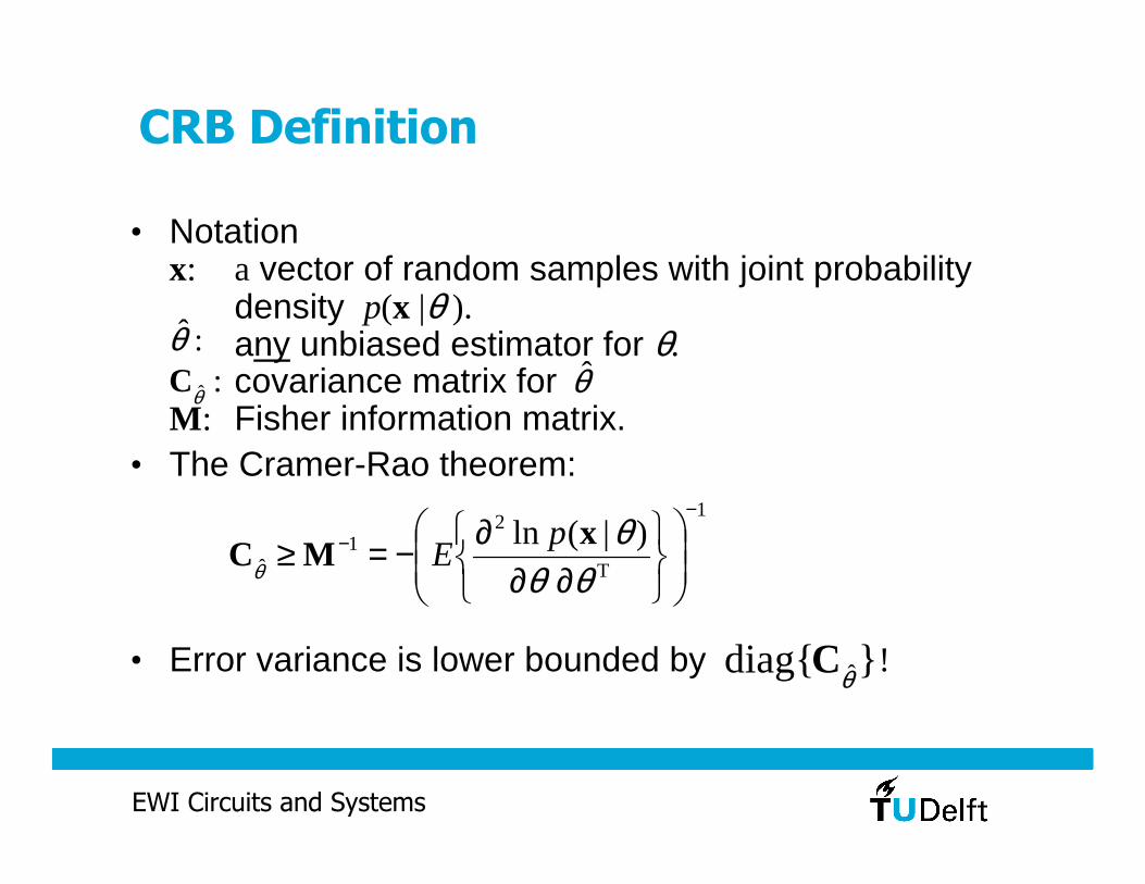
CRB Definition
• Notationx: a vector of random samples with joint probability
density p(x |θ ).any unbiased estimator for θ. covariance matrix for
M: Fisher information matrix.• The Cramer-Rao theorem:
• Error variance is lower bounded by !
:θ̂:θ̂C
1
T
21
ˆ
)|(ln−
−
∂∂∂−=≥
θθθx
MCp
Eθ
}diag{ θ̂C
θ̂

EWI Circuits and Systems
A Simple Example
• Estimate a constant in additive white Gaussian noise:
T]]1[,],0[[
][][
−=
+=
Nxx
nwnx
Lx
θ
+w[n] x[n]
θ
0 10 20 30 40 50 60 70 80 90 1000
1
2
3
4
5
6
7
8
9
10
n
x[n]
θ

EWI Circuits and Systems
A Simple Example
• Estimate a constant in additive white Gaussian noise:
.)ˆvar( Thus
)(
)|(ln,)][(
1)|(ln
)][(2
1exp
)2(
1)|(
21
2
22
21
02
1
0
222 2
N
NE
Npnx
p
nxp
N
n
N
nN
σσ
θ
σθθθ
σθθ
θσπσ
θ
=
−−≥
−=∂
∂−=∂
∂
−−=
−
−
=
−
=
∑
∑
xx
x

EWI Circuits and Systems
A Simple Example
• Estimate a constant in additive white Gaussian noise:
.)ˆvar( Thus
)(
)|(ln,)][(
1)|(ln
)][(2
1exp
)2(
1)|(
21
2
22
21
02
1
0
222 2
N
NE
Npnx
p
nxp
N
n
N
nN
σσ
θ
σθθθ
σθθ
θσπσ
θ
=
−−≥
−=∂
∂−=∂
∂
−−=
−
−
=
−
=
∑
∑
xx
x
This looks very familiar!

EWI Circuits and Systems
A Simple Example
• This proves what we already knew: you can’t beat the sample mean estimator
• In general, relationships to parameters of interest are complex, and we do not know analytically.
• CRB must be evaluated to bound the problem.
Nnx
NEnx
N
N
n
N
n
22
21
0SM
1
0SM ][
1)ˆvar(,][
1ˆ σθθθ =−
== ∑∑−
=
−
=
)ˆvar(θ

EWI Circuits and Systems
A Second Simple Example
• Line fitting in additive white Gaussian noise:
][][ 21 nwnnx ++= θθ
+w[n] x[n]
θ1+θ2n
0 10 20 30 40 50 60 70 80 90 1003
4
5
6
7
8
9
10
11
n
x[n]
θ1
θ2
We now have no intuition on estimation error for θ1 and θ2!

EWI Circuits and Systems
A Second Simple Example
221
21
0
222
2
21
02
21
2
1
0212
2
1
0212
1
1
0
22122
)|(ln,
1)|(ln,
1)|(ln
)][(1)|(ln
,)][(1)|(ln
)][(2
1exp
)2(
1)|(
2
σθσθσθθ
θθσθ
θθσθ
θθσπσ
Npn
pn
p
nnnxp
nnxp
nnxp
N
n
N
n
N
n
N
n
N
nN
−=∂
∂−=∂
∂−=∂∂
∂
+−=∂
∂+−=∂
∂
+−−=
∑∑
∑∑
∑
−
=
−
=
−
=
−
=
−
=
θθθ
θθ
θ
xxx
xx
x

EWI Circuits and Systems
• Variance on constant term θ1 is now higher. → estimating more parameters increases error.
• Variance of slope term, θ2, drops more rapidly with N.→ θ2 is easier to estimate. → x[n] is more sensitive to θ2 due to multiplication by n.
A Second Simple Example: Insights
[ ] [ ])1(
12)var(,
)1(
)12(2)var(
,
6
)12)(1(
2
)1(2
)1(1
2
2
2,21
2
2
1,11
1
2
−==
+−==
−−−
−
=
−−
NNNN
N
NNNNN
NNN
σθσθ
σ
MM
M
3
2
2
2
1
12)var(lim
4)var(lim
NN NN
σθσθ ≥≥∞→∞→

EWI Circuits and Systems
What algorithm do we use?
• What estimator achieves the CRB?• Maximum likelihood (ML) does asymptotically (N→∞).
• Consider our second example:
)|(lnmaxargˆML θθ
θxp=
−
−
−=
=
=+−=∂
∂=+−=∂
∂
∑
∑
∑∑
∑
∑∑
−
=
−
=−
=
−
=
−
=
−
=
−
=
1
0
1
01
0
21
0
1
0
2
1ML
1
0212
2
1
0212
1
][
][1
ˆ
ˆˆ
0)][(1)|(ln
,0)][(1)|(ln
N
n
N
nN
n
N
n
N
n
N
n
N
n
nnx
nx
nn
nN
nnnxp
nnxp
θθ
θθσθ
θθσθ
θ
θθ xx
Unfortunately ML is not practical for LOFAR calibration

EWI Circuits and Systems
CRB Uses in Radio Astronomy
1. Calibration algorithm development and assessment
• Is the existing algorithm adequate?
• Is there hope for finding a better solution?
• Permits trading off performance and computational burden. Answers “How close are we?”
• Faster than simulation, more flexible than direct observation.
• Can be computed even if no algorithm exists yet.

EWI Circuits and Systems
CRB Uses in Radio Astronomy
2. Performance Prediction in real observations
• The bound is specific to signal conditions.
• Can forewarn an astronomer of poor calibration conditions.
• A real-time tool could be developed. “Will this observation work?”

EWI Circuits and Systems
Direction Dependent Calibration
•Each station sees a differentdirection dependent blur.•Calibration on several brightpoint sources in the field of view is required.
x
G
K
m=1 m=M

EWI Circuits and Systems
Direction Dependent CalibrationData Model
V: visibility matrix, computed over a series of time-frequency intervals. Observed.
G: calibration complex gain matrix. One column per calibrator source. Unknown.
K: Fourier kernel, geometric array response. sq is source direction vector. rm is station location. Known.
B: Calibrator source intensity. Known.
D: Noise covariance. Unknown.
=
=
⋅=
=
=
+⋅⋅==
MQ
mqcf
qm
QMM
Q
QMM
Q
d
d
b
b
ik
kk
kk
gg
gg
nnE
OO
L
MM
L
L
MM
L
oo
11
2,
,1,
,11,1
,1,
,11,1
H
H
,
}exp{,
)()(
]}[][{
DB
rsK
G
DKGBKG
xxV
π

EWI Circuits and Systems
CRB for Calibration Parameters
• For the general multivariate Gaussian case the Fisher information has a nice closed form:
• For LOFAR V(θ) is the visibility (covariance) matrix for full array sample vector x.
• θ contains unknown gains and phases for Q calibrator sources, and noise powers for each station:
[ ]T0
10
100
H ))((vec)(),())(())(()(
θθθθθθ
∂∂=⊗= −− V
FFVVFM θ
T11
TTTT
],,,,[
]}vec{,}vec{,}|vec{|[
d
DGG
QQ ϕϕγγ
θ
LL=
∠=

EWI Circuits and Systems
Applying Parameter Model Constraints
• Performance improves by estimating a smaller set of constrained parameters, p. θ = f(p).
• Constraint examples:• Compact core sees coherent scene.• Phase is a deterministic function of frequency.• Smoothing polynomial over time-frequency-space.
• Vk,n are statistically independent over time-frequency. Each bin (k,n) has distinct Mk,n and θk,n.
T,
,,,1 1
H,
)(,
p
pJJMJMp ∂
∂==∑∑
= =
nknknknk
K
k
N
nnk
θEnforcesconstraint

EWI Circuits and Systems
Now it Gets a Little Messy
O
Constraint Jacobian for packed central core
Block Fisher information
Blockclosedforms

EWI Circuits and Systems
Now it Gets a Little Messy
The important points:• Closed form CRB expressions have been derived for
most important LOFAR calibration models.• Though expressions are complex, computer codes
have been developed to evaluate them.• These solutions exist now and could be made available
for astronomers to predict calibration performance for a given observations.

EWI Circuits and Systems
The Single Snapshot LOFAR Calibration Ambiguity
• For conventional arrays without direction dependent ionospheric phase perturbation calibration is possible with one Vk,n observation.
• Not so for LOFAR, there is an essential ambiguity.
• CRB blows up, M is singular!
1
H
HH
))(()(~
matrixunitary a ,
)()(
21
21
21
21
−•− ⋅⋅=
=
+⋅⋅=
KBUBKGUG
IUU
DKGBUUBKGV
oo
oo Rotation by U is invisible in V
Each U produces a different calibration

EWI Circuits and Systems
Solutions to Calibration Ambiguity
• Time-frequency diversity• Fringe rotation over time and across bands changes visibility
structure while calibration gains are relatively constant.• Cells, Snippets, Polc’s, UV Bricks, Peeling.• Low order polynomial fitting.• Peeling.
• Single snapshot calibration• Compact core.• Deterministic Frequency dependence.• Known gain magnitudes.
• CRB analysis is completed for most of these scenarios.

EWI Circuits and Systems
LOFAR Calibration with Compact Central Core
• Though phase distortion is direction depen-dent, each station sees the same ionosphere.
• Central core sees a coherent scene, imaging is possible
• One calibration gain is estimated for each station.
Station beamfield of view
Ionosphere
Closely packed LOFAR stations
Phase and gain isdirection dependentbut stations see thesame ionosphere

EWI Circuits and Systems
LOFAR Calibration with Compact Central Core
• The full array can be calibrated given a compact central core.• The wisdom of the LOFAR design is confirmed by CRB analysis
-1 -0.8 -0.6 -0.4 -0.2 0 0.2 0.4 0.6 0.8 1
x 105
-1
-0.8
-0.6
-0.4
-0.2
0
0.2
0.4
0.6
0.8
1x 10
5
-3000 -2000 -1000 0 1000 2000 3000-3000
-2000
-1000
0
1000
2000
3000
Full array Compact core

EWI Circuits and Systems
LOFAR Calibration with Compact Central Core (Optional slide instead of last)
• Calibration succeeds for Q ≤ Mc+1. Q calibrator sources and an Mc element core.
0 10 20 30 40 50 60 70 80 900
0.5
1
1.5
2
2.5
3
3.5
4
4.5
5x 10
12 CRB for 10 element array,4 element subarray and 6 sources
Mea
n S
quar
ed E
rror
Parameter Index
CRBstart of phasesstart of noise powers
0 5 10 15 20 25 30 35 40 45 500
0.5
1
1.5x 10
−3 MSE for 10 element array,4 element subarray and 3 sources
Mea
n S
quar
ed E
rror
Parameter Index
ML Monte CarloCRBstart of phasesstart of noise powers
×1012×10-3

EWI Circuits and Systems
2-D Polynomial Model over time-frequency for Ionospheric Variation
• Variations in G are smooth over time and frequency
• We have CRB analysis for 2-D polynomial interpolation:
{ })(exp
)(
112
02012
201000
112
02012
201000,
nknnkk
nknnkknk
tfttffi
tfttff
ΦΦΦΦΦΦ
ΓΓΓΓΓΓ
+++++
+++++=
⋅oG
[ ]TT11
T00
T11
T00 }diag{,}vec{,,}vec{,}vec{,,}vec{ Dp ΦΦΓΓ LL=

EWI Circuits and Systems
Full Sky Map
3C461
3C144
3C405
3C147
3C274
Full Sky Map

EWI Circuits and Systems
Field of View
6667686970717254
54.5
55
55.5
56
56.5
57
4C+55.08
4C+54.06
4C+56.09
4C+56.10
4C+55.09
Field of View
Right Ascension (deg)
Dec
linat
ion
(deg
)
EWI Circuits and Systems
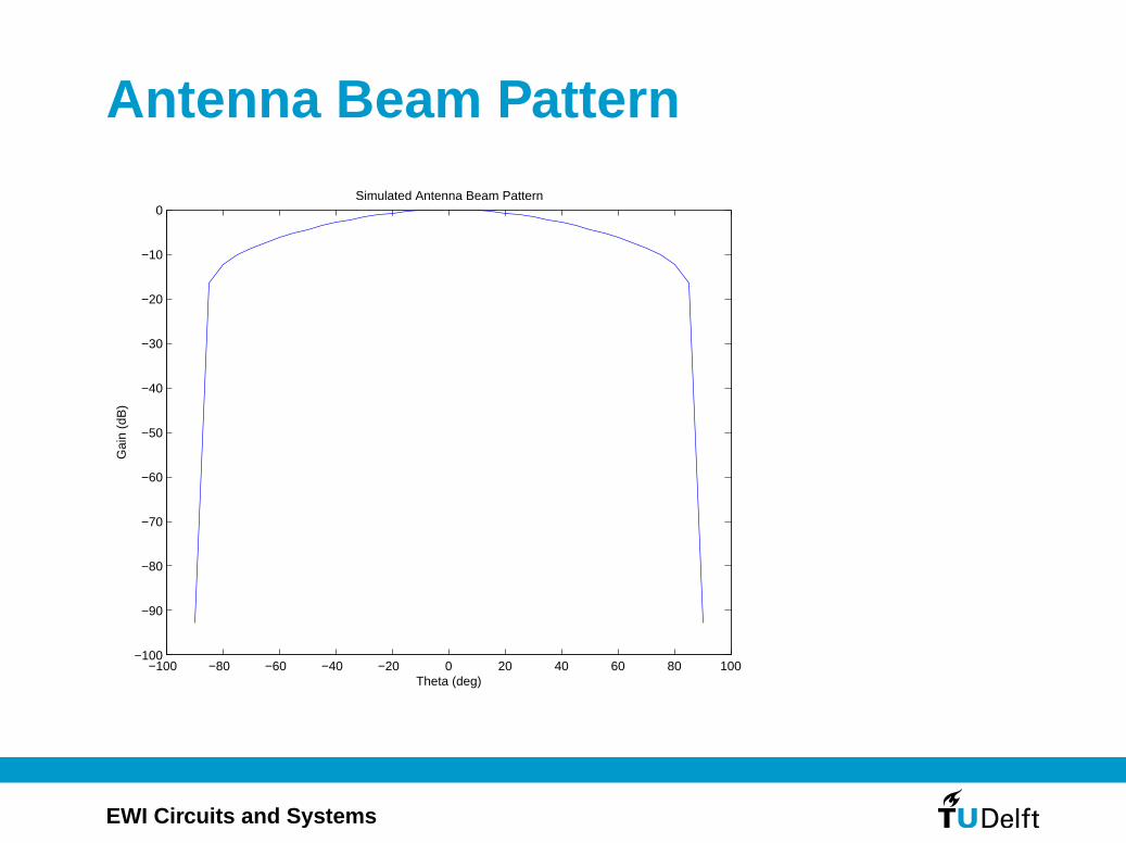
Antenna Beam Pattern
−100 −80 −60 −40 −20 0 20 40 60 80 100−100
−90
−80
−70
−60
−50
−40
−30
−20
−10
0Simulated Antenna Beam Pattern
Theta (deg)
Gai
n (d
B)
EWI Circuits and Systems
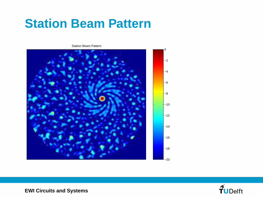
Station Beam Pattern
Station Beam Pattern
−20
−18
−16
−14
−12
−10
−8
−6
−4
−2
0

EWI Circuits and Systems
Noise
Assume sky noise limited and 550K @ 90 MHz
Tsky ∼ λ2.7
Rayleigh-Jeans law
B =2kT
λ2
Integration over a hemisphere
Pnoise = 2πB

EWI Circuits and Systems
Source power & SNR
Source powers from 3C & 4C catalogs @178MHz.Assume all sources have spectral index α = 0.7,then
Psource ∼ λ0.7
The Signal to Noise Ratio (SNR) does not change
with frequency.
EWI Circuits and Systems
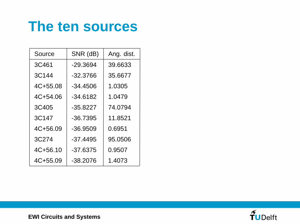
The ten sources
Source SNR (dB) Ang. dist.
3C461 -29.3694 39.6633
3C144 -32.3766 35.6677
4C+55.08 -34.4506 1.0305
4C+54.06 -34.6182 1.0479
3C405 -35.8227 74.0794
3C147 -36.7395 11.8521
4C+56.09 -36.9509 0.6951
3C274 -37.4495 95.0506
4C+56.10 -37.6375 0.9507
4C+55.09 -38.2076 1.4073

EWI Circuits and Systems
Single source calibration - constant gain
Time (s)
Fre
quen
cy (
kHz)
Gain error − Antenna m=1 / Source = 4C+55.08 / Q = 1
1 2 3 4 5 6 7 8 9 10 11
50
100
150
200
250
300
350
400
450
500−15
−10
−5
0
5
10
15
20

EWI Circuits and Systems
Multiple sources - constant gain
Time (s)
Fre
quen
cy (
kHz)
Gain error − Antenna m=1 / Source q=3 (4C+55.08) / Q = 10
1 2 3 4 5 6 7 8 9 10 11
50
100
150
200
250
300
350
400
450
500
−10
0
10
20
30
40
50
60

EWI Circuits and Systems
Multiple sources - constant gain
Time (s)
Fre
quen
cy (
kHz)
Relative gain error − Antenna m=1 / Source q=3 (4C+55.08)
1 2 3 4 5 6 7 8 9 10 11
50
100
150
200
250
300
350
400
450
500
10
20
30
40
50
60
70
80
90
100

EWI Circuits and Systems
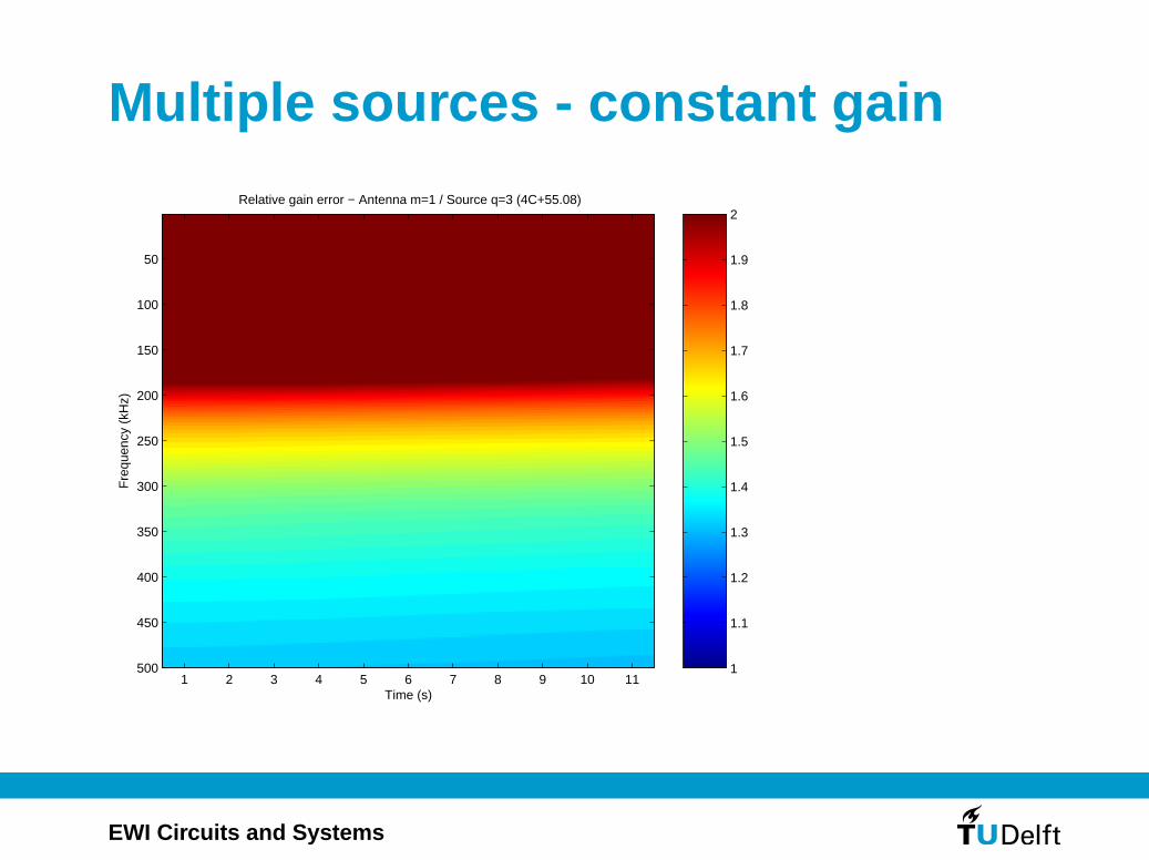
Multiple sources - constant gain
Time (s)
Fre
quen
cy (
kHz)
Relative gain error − Antenna m=1 / Source q=3 (4C+55.08)
1 2 3 4 5 6 7 8 9 10 11
50
100
150
200
250
300
350
400
450
500
2
4
6
8
10
12
14
16
18
20
EWI Circuits and Systems
Multiple sources - constant gain
Time (s)
Fre
quen
cy (
kHz)
Relative gain error − Antenna m=1 / Source q=3 (4C+55.08)
1 2 3 4 5 6 7 8 9 10 11
50
100
150
200
250
300
350
400
450
500 1
1.1
1.2
1.3
1.4
1.5
1.6
1.7
1.8
1.9
2

EWI Circuits and Systems
Multiple sources - 2D polynomial
Time (s)
Fre
quen
cy (
kHz)
Relative gain error (a0) − Antenna m=1 / Source q=3 (4C+55.08)
1 2 3 4 5 6 7 8 9 10 11
50
100
150
200
250
300
350
400
450
500
10
20
30
40
50
60
70
80
90
100

EWI Circuits and Systems
Multiple sources - 2D polynomial
Time (s)
Fre
quen
cy (
kHz)
Relative gain error (a0) − Antenna m=1 / Source q=3 (4C+55.08)
1 2 3 4 5 6 7 8 9 10 11
50
100
150
200
250
300
350
400
450
500
2
4
6
8
10
12
14
16
18
20

EWI Circuits and Systems
Multiple sources - 2D polynomial
Time (s)
Fre
quen
cy (
kHz)
Relative gain error (a1) − Antenna m=1 / Source q=3 (4C+55.08)
1 2 3 4 5 6 7 8 9 10 11
50
100
150
200
250
300
350
400
450
500
10
20
30
40
50
60
70
80
90
100

EWI Circuits and Systems
Multiple sources - 2D polynomial
Time (s)
Fre
quen
cy (
kHz)
Relative gain error (a1) − Antenna m=1 / Source q=3 (4C+55.08)
1 2 3 4 5 6 7 8 9 10 11
50
100
150
200
250
300
350
400
450
500
2
4
6
8
10
12
14
16
18
20

EWI Circuits and Systems
Multiple sources - 2D polynomial
Time (s)
Fre
quen
cy (
kHz)
Relative gain error (a2) − Antenna m=1 / Source q=3 (4C+55.08)
1 2 3 4 5 6 7 8 9 10 11
50
100
150
200
250
300
350
400
450
500
10
20
30
40
50
60
70
80
90
100

EWI Circuits and Systems
Multiple sources - 2D polynomial
Time (s)
Fre
quen
cy (
kHz)
Relative gain error (a2) − Antenna m=1 / Source q=3 (4C+55.08)
1 2 3 4 5 6 7 8 9 10 11
50
100
150
200
250
300
350
400
450
500
2
4
6
8
10
12
14
16
18
20

EWI Circuits and Systems
Limitations to Current CRB Analysis
• So far it includes only error effects due to noise and sample covariance estimation.
• There can also be modeling errors, e.g. maybe a polynomial fits time-frequency variation poorly.
• Errors in tabulated source location and brightness are not considered.
• Array station location is assumed to be exact.
• Station calibration errors are lumped in with ionospheric gains.
EWI Circuits and Systems
Conclusions
• The BIG answer: Yes, LOFAR can be calibrated
• Given a range of time-frequency observations and compact core geometry: there are no theoretical roadblocks to achieving useful calibration estimates.
• If an algorithm can be developed to approach the CRB calibration error should be acceptable.