THEORETICAL INVESTIGATION ON THE EFFECT OF FLUID …

TKK Dissertations 80Espoo 2007

THEORETICAL INVESTIGATION ON THE EFFECT OF FLUID FLOW BETWEEN THE HULL OF A SHIP AND ICE FLOES ON ICE RESISTANCE IN LEVEL ICEDoctoral Dissertation

Helsinki University of TechnologyDepartment of Mechanical EngineeringLaboratory for Mechanics of Materials

Jorma Kämäräinen

TKK Dissertations 80Espoo 2007

Dissertation for the degree of Doctor of Science in Technology to be presented with due permission of the Department of Mechanical Engineering for public examination and debate in Auditorium K216 at Helsinki University of Technology (Espoo, Finland) on the 21st of September, 2007, at 12 noon.

Helsinki University of TechnologyDepartment of Mechanical EngineeringLaboratory for Mechanics of Materials

Teknillinen korkeakouluKonetekniikan osastoLujuusopin laboratorio

Jorma Kämäräinen

THEORETICAL INVESTIGATION ON THE EFFECT OF FLUID FLOW BETWEEN THE HULL OF A SHIP AND ICE FLOES ON ICE RESISTANCE IN LEVEL ICEDoctoral Dissertation

Distribution:Helsinki University of TechnologyDepartment of Mechanical EngineeringLaboratory for Mechanics of MaterialsP.O. Box 4300FI - 02015 TKKFINLANDURL: http://www.tkk.fiTel. +358-9-451 3441Fax +358-9-451 3449E-mail: [email protected]

© 2007 Jorma Kämäräinen

ISBN 978-951-22-8860-1ISBN 978-951-22-8861-8 (PDF)ISSN 1795-2239ISSN 1795-4584 (PDF) URL: http://lib.tkk.fi/Diss/2007/isbn9789512288618/

TKK-DISS-2322

Multiprint OyEspoo 2007

AB

ABSTRACT OF DOCTORAL DISSERTATION HELSINKI UNIVERSITY OF TECHNOLOGY P.O. BOX 1000, FI-02015 TKK http://www.tkk.fi

Author Jorma Kämäräinen

Name of the dissertation Theoretical Investigation on the Effect of Fluid Flow between the Hull of a Ship and Ice Floes on Ice Resistance in Level Ice

Manuscript submitted 9 June 2006 Manuscript revised 31 May 2007

Date of the defence 21 September 2007

Monograph Article dissertation (summary + original articles)

Department Department of Mechanical Engineering Laboratory Laboratory for Mechanics of Materials Field of research Mechanics of Materials Opponent(s) Professor Jari Hämäläinen and Dr. Petri Valanto Supervisor Professor Jukka Tuhkuri Instructor Emeritus Professor Eero-Matti Salonen

Abstract The icebreaking capability of a ship in level ice is a very important concept for the designers of ice-going ships. The increase of ice resistance with speed is both due to the increase in the resistance forces with speed in the ice-breaking phase, which takes place at the waterline level, and in the sliding phase when the broken ice floes are submerged. The resistance of a ship in level ice as a result of the decrease in pressure between the hull surface and an ice floe when the ice floe is submerged is studied in this thesis. Three basic phenomena have been presented in the literature to explain the origin of the change of the pressure in the gap between the hull and an ice floe in the sliding phase: the ventilation phenomenon; the acceleration of water flow in the gap between the ice floe and the hull surface, and the flow of water to and from the gap as a result of changes in the geometry of the hull along the trajectory of an ice floe sliding against the hull. The research objective of this study was to study the effect of the last two phenomena on ice resistance in the sliding phase and to develop a calculation tool for this purpose. The CFD code Iceflo based on the hydrodynamic lubrication theory was written to calculate the flow in the gap between the hull surface and an ice floe. The following main conclusions can be drawn. The low-pressure phenomenon in the gap between the hull surface and ice floes may be caused by the inertia forces under favourable conditions or by changes in the height of the gap between the hull surface and the ice floes, or both. The force resulting from the pressure decrease in the gap between the hull surface and ice floes may be several times the force resulting from the static lift of the ice floes. This phenomenon has to be taken into account e.g. in friction panel tests. The resistance caused by the low pressure in the gap is higher than the resistance resulting from viscous forces in the gap. An inclined cylindrical bow form can be considered to be the optimal hull form for an icebreaking ship, concerning the low-pressure phenomenon. Keywords Ice resistance, computational fluid dynamics, hydrodynamic lubrication theory

ISBN (printed) 978-951-22-8860-1 ISSN (printed) 1795-2239

ISBN (pdf) 978-951-22-8861-8 ISSN (pdf) 1795-4584

Language English Number of pages 157

Publisher Helsinki University of Technology, Laboratory for Mechanics of Materials

Print distribution Helsinki University of Technology, Laboratory for Mechanics of Materials

The dissertation can be read at http://lib.tkk.fi/Diss/2007/isbn9789512288618/

VÄITÖSKIRJAN TIIVISTELMÄ TEKNILLINEN KORKEAKOULU PL 1000, 02015 TKK http://www.tkk.fi

Tekijä Jorma Kämäräinen

Väitöskirjan nimi Teoreettinen tutkimus laivan rungon ja jäälohkareiden välisen nestevirtauksen vaikutuksesta jäävastukseen tasaisessa jäässä

Käsikirjoituksen päivämäärä 9.6.2006 Korjatun käsikirjoituksen päivämäärä 31.5.2007

Väitöstilaisuuden ajankohta 21.9.2007

Monografia Yhdistelmäväitöskirja (yhteenveto + erillisartikkelit)

Osasto Konetekniikan osasto Laboratorio Lujuusopin laboratorio Tutkimusala Lujuusoppi Vastaväittäjä(t) professori Jari Hämäläinen ja PhD Petri Valanto Työn valvoja professori Jukka Tuhkuri Työn ohjaaja emeritus professori Eero-Matti Salonen

Tiivistelmä Laivan tasaisen jään murtokyky on hyvin tärkeä käsite jäissä kulkevien alusten suunnittelijoille. Jäävastuksen kasvu nopeuden kasvaessa johtuu sekä vastusvoimien kasvusta jään murtovaiheessa, joka tapahtuu vesiviivan tasolla, että liukuvaiheessa, kun murretut jäälohkareet upotetaan. Tässä väitöskirjassa tutkitaan tasaisessa jäässä liikkuvan laivan jäävastusta, joka aiheutuu laivan runkopinnan ja jäälohkareen välisen paineen alenemisesta, kun jäälohkare upotetaan. Kirjallisuudessa on esitetty kolme ilmiötä upotusvaiheessa ilmenevän rungon ja jäälohkareen välisen paineen muutoksen synnyn selittämiseksi: ventilaatioilmiö, veden virtauksen kiihtyminen jäälohkareen ja rungon välisessä raossa ja veden virtaus rakoon ja raosta pois, joka johtuu rungon geometrian muutoksista runkoa vasten liukuvan jäälohkareen kulkureitillä. Tämän tutkimuksen tarkoituksena oli selvittää kahden viimeksi mainitun ilmiön vaikutusta jäävastukseen liukuvaiheessa ja kehittää tätä tarkoitusta varten laskentatyökalu. Runkopinnan ja jäälohkareen välisen virtauksen laskentaa varten kirjoitettiin tietokoneohjelma Iceflo, joka perustuu hydrodynaamiseen voiteluteoriaan. Tutkimuksen tärkeimmät johtopäätökset ovat seuraavia. Runkopinnan ja jäälohkareiden välisessä raossa ilmenevä alipaineilmiö voi suotuisissa olosuhteissa johtua hitausvoimista tai runkopinnan ja jäälohkareiden välisen raon korkeuden muutoksista tai molemmista syistä. Voima, joka aiheutuu paineen alenemisesta runkopinnan ja jäälohkareiden välisessä raossa, voi olla useita kertoja suurempi kuin voima, joka aiheutuu jäälohkareiden staattisesta nosteesta. Tämä ilmiö on otettava huomioon mm. kitkapanelikokeissa. Raossa syntyvästä alipaineesta aiheutuva vastus on suurempi kuin raossa syntyvien nestekitkavoimien aiheuttama vastus. Kallistettua sylinterimäistä keulamuotoa voidaan pitää optimaalisena jäätämurtavan aluksen runkomuotona alipaineilmiön kannalta.

Asiasanat Jäävastus, laskennallinen virtausmekaniikka, hydrodynaaminen voiteluteoria

ISBN (painettu) 978-951-22-8860-1 ISSN (painettu) 1795-2239

ISBN (pdf) 978-951-22-8861-8 ISSN (pdf) 1795-4584

Kieli englanti Sivumäärä 157

Julkaisija Teknillinen korkeakoulu, Lujuusopin laboratorio

Painetun väitöskirjan jakelu Teknillinen korkeakoulu, Lujuusopin laboratorio

Luettavissa verkossa osoitteessa http://lib.tkk.fi/Diss/2007/isbn9789512288618/

AB

iii

Preface and acknowledgements I first became interested in the resistance of ships in level ice when I was involved in the design of ice-going cargo ships at the Valmet Helsinki Shipyard in Finland at the beginning of the 1980s. It could be noted that resistance in level ice is much higher than resistance in open water. In particular, the very considerable linear increase in ice resistance with speed urged theoretical explanation. The existing empirical formulae basically divided ice resistance in level ice into two components: resistance caused by ice breaking and that caused by ice submerging (see e.g. Kämäräinen (1993a)). In Valanto’s (1989) experiments with a simple two-dimensional model it was found that the ice-breaking resistance component did not seem to increase with speed. On the basis of this observation I developed my own empirical calculation method for the calculation of a ship’s ice resistance in level ice (Kämäräinen (1993a)), which gave a good correlation with full-scale data. However, I could not find any physical phenomenon which could explain the increase in ice resistance with speed as a result of ice submerging. The problem bothered me and finally I got the idea of studying the pressure field between the hull of the ship and the ice floes (Kämäräinen (1993b)). The squat phenomenon is a well-known problem for sailors. The squat phenomenon may exist when a ship is sailing on a fairway with a small clearance between the bottom of the ship and the sea bottom. If the speed of the ship is high enough, the bottom of the ship may touch the sea bottom as a result of loss of pressure between the hull and the sea bottom caused by the Bernoulli effect. There was strong reason to believe that a similar type of pressure decrease phenomenon could also exist between the hull and the ice floes when the ship is sailing in level ice. In 1999 I met Mr. Jens-Holger Hellmann of HSVA at a meeting in London, and learned that Mr. Fernando Puntigliano had independently developed similar ideas at HSVA with Dr. Petri Valanto. This information inspired me to continue my research related to the pressure decrease phenomenon in August 2000, when I joined the Laboratory of Mechanics of the Helsinki University of Technology (HUT). My warm thanks go to Emeritus Professor Martti Mikkola, who accepted me to join his staff. I would also like to thank the personnel of the Laboratory of Mechanics for the good working atmosphere during my stay at the University in 2000-2002. The help of Mr. Timo Teinonen in keeping my computer system "alive" is acknowledged. I would also like to thank the Laboratory of Physics of HUT for providing good working premises during the final preparation of my thesis in 2003-2007. The lectures of Professor Timo Siikonen at the Helsinki University of Technology on computational fluid dynamics (CFD) were very valuable for me when preparing the Iceflo computer code. Some sub-routines of the code were borrowed from his exercises related to his lectures on CFD. My sincere thanks go to CSC (Tieteellinen laskenta Oy) for their permission to use the CEDAR computer and the Fluent CFD computer code for my calculations when preparing the thesis. The help for the use of Fluent of Dr. Thomas Zwinger of CSC is gratefully acknowledged.

iv

I would like to thank Dr. Fernando Puntigliano for our warm and fruitful discussions on the pressure decrease phenomenon in 1999 in Helsinki and in 2000 in Hamburg. Without his model test results and ideas related to the pressure decrease phenomenon I would probably not have continued my studies on the matter. The pre-examiners of this thesis were Docent Hannu Ahlstedt and Dr. Petri Valanto. I would like to thank them for their valuable comments and suggestions on my thesis. I would also like to thank Professor Jukka Tuhkuri for his comments on my thesis. The Maritime Foundation of Finland (Merenkulun säätiö) and the Laboratory for Mechanics of Materials of HUT are acknowledged for the financial support for my thesis and the Finnish Maritime Administration for accepting my leave of absence from my duties at the Administration in 2000-2002. Ruth Vilmi Online Education Ltd is acknowledged for reviewing the English language. Finally, my warmest thanks go to Emeritus Professor Eero-Matti Salonen, who has been my advisor in my studies on the pressure decrease phenomenon since 1993. Without his continuous and patient advice, encouragement, and support it would not have been possible for me to finalise my thesis. I also want to thank warmly my family and friends who have supported me in ups and downs on the long road. Vantaa, 31 May 2007 Jorma Kämäräinen

v

Table of contents Abstract of Doctoral Dissertation i Väitöskirja tiivistelmä ii Preface and acknowledgements iii Table of contents v List of abbreviations ix List of frequently used symbols x 1 Introduction ……..………………………………………………….………..1

1.1 Description of the icebreaking process in level ice …………................ 1 1.2 Definition of level ice resistance of a ship …………….…………............ 2 1.3 Components of ice resistance in level ice ……………….….………….… 3 1.4 Ice resistance resulting from the sliding phase ……………………..……. 5 1.5 Hull-ice interaction forces in the sliding phase ………………………..… 6 1.6 The effect of change in pressure below an ice floe on ice resistance in the sliding phase …………………………………………..………… 8 1.7 The effect of change in pressure between the hull surface and an ice floe

on ice resistance in the sliding phase ……………….………………….. 10 1.7.1 Change in pressure between the hull and an ice floe, according to

Enkvist ……..……………….…………...……............................. 10 1.7.2 Change in pressure between the hull and an ice floe, according to the author …….……..…….…….............................................. 11 1.7.3 Change in pressure between the hull and an ice floe, according

to Puntigliano …………………………..…...…………………... 11 1.7.4 The effect of change in pressure above an ice floe on ice

resistance in the sliding phase …………………………………… 12 1.7.4.1 Normal and tangential forces acting on the hull ……....….12 1.7.4.2 Ice resistance resulting from the sliding phase ………....... 13

1.8 The research objective ……………………………………….……….… 13 2 Model- and full-scale test data……………………………...……………14 2.1 Model-scale test data ………………………………………………. 14

2.1.1 Model tests of Liukkonen with a two-dimensional model …......... 14 2.1.2 Model tests of Kayo with a segmented model …………….……... 16 2.1.3 Model tests of Puntigliano with a simplified Waas bow ……..... 19 2.1.4 Model tests of Puntigliano with a cylindrical bow ……….……. 24 2.1.5 Model tests on hull-ice contact ………………………..…….... 27

2.2 Full-scale and model-scale test data with MPV Neuwerk………….... 30 2.2.1 Full-scale test data ………………………….………………….... 30 2.2.2 Model-scale test data ……………………….………………….... 32

2.3 Data on the size of ice floes on a full scale ………………………..…… 33 2.4 Radii of curvature of real hull surfaces …………………….…………. 34

vi

2.5 Surface roughness of the hull and ice surfaces ………………….......... 36 2.6 Summary of Chapter 2 ………………………………………….……... 38

3 Definition of the calculation problem and outline of the solution

methods ………………………………………………………………..…… 39 3.1 The governing equations ……………………………………………... 39

3.1.1 Turbulence modelling …………………………………….…. 40 3.1.2 Reynolds averaging ………………………………………..... 41

3.2 Analysis of the calculation problem …………………………………... 42 3.3 Outline of the solution methods ……………………………………..... 47

4 The Fluent computational fluid dynamics computer code ……………. 48 4.1 The Fluent CFD computer code ………………………………………. 48

4.1.1. The standard k ε− turbulence model used by Fluent ……….... 49 4.1.1.1 Transport equations for the standard k ε− model ............. 49 4.1.1.2 Modelling turbulent production in the k ε− model …... 49 4.1.1.3 Modelling the turbulent viscosity ……………………… 50 4.1.1.4 Model constants ………………………………….…….. 50

4.2 Validation of Fluent …………………………………………………... 50 4.2.1 Validation of the turbulence models of Fluent ………………….51

4.2.1.1 Comparison of the calculated shear stresses with the data of Bech et al. …………………………………………...53 4.2.1.2 Results of the standard k ε− model of Fluent ………….53

4.2.2 Comparison of the results obtained by Fluent with the experimental data of the turbulent Couette-type flow of Nakabayashi …………………………………………………….57

4.2.2.1 Description of the flow ……………………………….....58 4.2.2.2 Comparison of the velocity magnitudes …………………..59 4.2.2.3 Comparison of turbulence kinetic energy …………….......60 4.2.2.4 Comparison of the friction velocities …………………...61 4.2.2.5 Comparison of the pressure gradients …………………..62

4.3 Summary of Chapter 4 …………………………………………………62

5 Hydrodynamic lubrication theory ……………………………………....63 5.1 Hydrodynamic lubrication theory for a three-dimensional flow without inertia effects …………………..…………………………………….64

5.2 Hydrodynamic lubrication theory for a three-dimensional flow with inertia effects ………………….………………………………………..65

5.2.1 Integration of the continuity equation …………………………….66 5.2.2 Integration of the momentum equations ………………………….67 5.2.3 The equations of Constantinescu …………………………………69 5.2.4 The turbulence models ……………………………………………70 5.2.5 Flow film cavitation ………………………………………………72 5.2.6 Flow film separation ……………………………………………...72

5.3 Numerical solution of the equations of Constantinescu ……………….73 5.3.1 Solution of the momentum equations …………………………….74 5.3.2 Solution of the Poisson-type equation ……………………………77 5.3.3 The outer iteration …………………………………………..........78 5.3.4 The boundary conditions …………………………………………79

5.3.4.1 No-slip boundary condition ……………………………...79

vii

5.3.4.2 Symmetric or free-slip boundary condition ……………...81 5.3.4.3 Periodic boundary condition ……………………………..81 5.3.4.4 Inflow and outflow boundary conditions …………………82 5.3.4.5 Free-flow boundary condition …………………………….82 5.3.4.6 Dynamic boundary condition ……………………………..83

5.3.5 Numerical stability of the solution method …………………….85 5.4 Calculation of forces and moment resulting from pressure and shear stress …...……………………………………………………….….…85 5.5 Verification and validation of the Iceflo CFD code …………………...86

5.5.1 Verification of Iceflo against the analytical solution of Constantinescu for a two-dimensional flow between a rotating cylinder and an infinite wall ………………………………………86 5.5.2 Validation of Iceflo against Fluent for two-dimensional flow ……90

5.5.2.1 Laminar flow ……………………………………………...91 5.5.2.2 Turbulent flow ……………………………………………92

5.5.3 Validation of Iceflo for a three-dimensional flow ………………..94 5.5.4 Validation of Iceflo against a flow generated by infinitely wide parallel walls approaching or moving apart………………….96

5.6 Summary of Chapter 5 …………………………………………………99

6 Theoretical calculations ………………………………………….………100 6.1 Analysis of the flow between the hull and the ice floe with constant hull curvature ……………………..…………………………………….100

6.1.1 The flow between a "ball-shaped" hull form and a square-shaped ice floe ……………………………………………………………100

6.1.1.1 Case 1: No leakage occurs through the gaps between the edges of the ice floes ……………………………..……102 6.1.1.2 Case 2: Leakage occurs through the gap between the ice floes at the northern edge …...………………...…………..106

6.1.2 The effect of pressure below the ice floes on ice resistance due to the sliding phase ………………...……………………….…110 6.1.3 Variation of the computational parameters and the effect of the turbulence model on the results ………………………………111

6.1.3.1 Variation of the under-relaxation parameters …………..111 6.1.3.2 The effect of the grid density on the solution …………..113 6.1.3.3 The effect of the turbulence model on the results of the calculations ……………………………………………...114

6.1.4 Variation of the geometric parameters …………………………..114 6.1.4.1 Contact between the hull surface and the ice floe ….…....114 6.1.4.2 Minimum distance between the surfaces ………………..116 6.1.4.3 Variation of the size of the ice floe ……………………...117 6.1.4.4 Variation of the velocity of the hull surface ……………...119 6.1.4.5 Variation of the curvature of the hull surface …………...119 6.1.4.6 The effect of the inclination of the ice floe on the pressure in the gap ………………………………………………...120

6.2 Analysis of the flow between the hull and the ice floe with changing hull curvature …………………………………………………………122

6.2.1 Variation of the radii of the hull surface with time ……………...122 6.2.1.1 Zero relative velocity of the surfaces in the x-coordinate direction …………………………………………………122

viii

6.2.1.2 Non-zero relative velocity of the surfaces in the x-coordinate direction ………………………….……..123

6.2.2 The effect of the waviness of the hull surface …………………...124 6.3 The effect of the negative pressure in the gap on the magnitude of ice resistance in the sliding phase ………………………………………...125

6.4 Summary of Chapter 6 ………………………………………….……..126

7 Discussion ………………………………………………………………..128 7.1 The effect of hull and ice surface roughness on level ice resistance in

the sliding phase …...........................................................................128 7.1.1 The effect of hull surface roughness on level ice resistance in the

sliding phase ………………..…………………………………..128 7.1.2 The effect of ice surface roughness on level ice resistance in the sliding phase ….……………………………………………….128

7.2 Analysis of model test results given in Chapter 2 …………………….129 7.2.1 Analysis of the model tests of Liukkonen ……………………..129 7.2.1.1 The effect of viscous forces on ice resistance ……...……129 7.2.1.2 The effect of change in pressure in the gap between the model and ice floes on ice resistance ……………..…… 130 7.2.1.3 The effect of change in pressure below the ice floes on ice resistance ………………………………………….. 132 7.2.1.4 Summary ……………………………………………… 134 7.2.2 Analysis of the model tests of Kayo ……………………….......134 7.2.3 Analysis of the model tests of Puntigliano with a simplified Waas bow ……………………………………………………….135

7.2.3.1 Analysis of ice resistance of Segment No. 2 …………... 135 7.2.3.2 The possible reason for the change in pressure in the gap

between the model surface and ice floes ………………. 136 7.2.4 Analysis of the model tests of Puntigliano with a cylindrical bow ……………………………...……………………………..139

7.3 Calculations for real ships …………………………………………….140 7.3.1 Full-scale and model-scale tests of MPV Neuwerk …………….140 7.3.2 IB Kapitan Evdokimov ………………………………………..140 7.3.3 The optimal form of the hull for breaking level ice ……………141

7.4 The low-pressure phenomenon and friction panel tests ………………141 7.5 Comparison of calculations made on full scale and on model scale …. 142 7.6 Calculation of ice resistance of ships in level ice …………………….145 7.7 Summary of Chapter 7 ……………………………………...…………..146

8 Summary ……………………….………………………………….……..147

9 Conclusions ………………………………………………………………150

References ………………………………………………………………………..152

ix

List of abbreviations AIAA American Institute of Aeronautics and Astronautics AP Aft perpendicular ASLE American Society of Lubrication Engineers ASME American Society of Mechanical Engineers BEPERS Bothnian Experiment in Preparation for ERS-1 CFD Computational Fluid Dynamics CL Centre Line CSC Centre of Scientific Computing - Tieteellinen laskenta Oy CV Control Volume DNS Direct Numerical Simulation FP Fore perpendicular HSVA Hamburgische Schiffbau-Versuchsanstalt GmbH

(Hamburg Ship Model Basin) HUT Helsinki University of Technology IAHR International Association for Hydraulic Research IB Icebreaker ISO International Organization for Standardization ISOPE International Society of Offshore and Polar Engineers IT Information Technology LES Large Eddy Simulation MAC Marker-and-cell (method) MPV Multi-Purpose Vessel MV Motor Vessel OMAE Offshore Mechanics and Arctic Engineering PC Personal Computer POAC Port and Ocean Engineering under Arctic Conditions RMS Reynolds Stress Model RV Research Vessel SFS Finnish Standards Association SNAME Society of Naval Architects and Marine Engineers WARC Wärtsilä Arctic Research Centre

x

List of frequently used symbols A area of an ice floe, or [m2]

coefficent of the Poisson-type equation [1/m] Af waterline area of the bow area of the ship [m2] b breadth of a rectangular ice floe [m] B beam of the ship [m] D side height of the ship [m] E modulus of elasticity [Pa] F force [N] Fn sum of the normal contact forces between the hull surface

and an ice floe [N] Fμ frictional force [N] g acceleration of gravity [m/s2] h height of the gap between the hull surface and an ice floe [m] he equivalent ice thickness [m] hice level ice thickness [m] hs thickness of the snow cover on top of ice [m] H shape factor [-] i cell number in the x-coordinate direction [-] j cell number in the y-coordinate direction [-] k turbulence kinetic energy [m2/s2] k+ dimensionless turbulence kinetic energy [-] kx turbulence viscosity coefficient in the x-coordinate

direction [-] ky turbulence viscosity coefficient in the y-coordinate

direction [-] K second coefficient of viscosity [Pa ⋅ s] l length of a rectangular ice floe [m] LOA overall length of the ship [m] Lpp length of the ship between the perpendiculars [m] LWL waterline length of the ship [m] m mass of an ice floe [kg] M moment [Nm] p pressure [Pa]

dp dynamic pressure [Pa]

1dp average dynamic pressure in the gap between the hull surface and an ice floe [Pa]

2dp average dynamic pressure below an ice floe [Pa]

hp hydrostatic pressure [Pa]

1hp average static pressure above an ice floe [Pa]

2hp average static pressure below an ice floe [Pa] Q mass flow rate, or [kg/s] shear force [N] R radius of the curvature of the hull [m] Ra centreline average of surface roughness [m] ReC Couette Reynolds number [-]

xi

Reτ Reynolds number based on wall friction velocity [-] *Re Reduced Reynolds number [-]

Rice ice resistance of a ship in level ice [N] Row resistance of a ship in open water [N] Rs ice resistance of a ship in level ice caused by the

sliding phase [N] Rtot total resistance of a ship in level ice [N] t time [s] T draught of the ship, or [m] temperature [oC] u velocity of the flow in the x-coordinate direction [m/s] uτ friction velocity [m/s] u+ normalised velocity in viscous scale [-] U velocity of the hull surface [m/s] v speed of the ship, or [m/s]

velocity of the flow in the y-coordinate direction [m/s] V volume [m3] w velocity of the flow in the z-coordinate direction [m/s] x, y, z Cartesian co-ordinates [m] z+ normalised distance in viscous scale [-] Greek symbols α waterline angle of the bow, or [deg]

under-relaxation parameter [-] ijδ Kronecker delta symbol ( ijδ = 1 if i = j, otherwise ijδ = 0) [-]

ε dissipation rate of turbulence kinetic energy [m2/s3] η molecular viscosity [Pa ⋅ s]

tη turbulent viscosity [Pa ⋅ s] λ model scale factor, or [-] wave length [m] μ friction coefficient [-] ν kinematic viscosity, or [m2/s] Poisson coefficient [-] ρ density [kg/m3]

iceρ density of ice [kg/m3]

wρ density of water [kg/m3] ρΔ difference between the densities of water and ice [kg/m3] τ shear stress [N/m2] φ buttock angle of the bow vertical, [deg]

angle between the tangent to the stem and the horizontal at the contact point of the ice floe and the hull surface, or [deg] solution value

ψ angle between the normal to the bow and the vertical, or [deg] or stream function [m2/s]

xii

Subscripts av average i,j cell numbering index i,j,k Cartesian co-ordinates in i, j, and k directions E east fsc full-scale m mean max maximum min minimum msc model-scale N north P cell centre rms root mean square S south W west w wall x x-coordinate direction y y-coordinate direction z z-coordinate direction Superscripts (n) previous time level (n+1) new time level ' the fluctuating part of the Reynolds decomposition mean value ̂ non-dimensional value

vector

1

1 Introduction The purpose of this study is to investigate theoretically the pressure and viscous forces resulting from the flow in the gap between the hull of a ship and fully submerged ice floes over which the hull slides when the ship is moving at a constant speed in a level ice field. In practice ice-going ships, i.e. ships strengthened for navigation in ice, rarely encounter level ice fields, but they do exist in archipelago areas where the ice field does not move very much as a result of winds and currents, because the ice field is anchored to the islands. In open sea broken ice fields or ridged ice fields are normally encountered. However, the icebreaking capability of a ship is usually determined in a level ice field on a model scale and validated in level ice on a full scale. Thus the ice resistance of ships in level ice is a very important concept for the designers of ice-going ships. In this chapter the icebreaking process in level ice is first briefly described and the components of ice resistance are introduced. Ice resistance in the sliding phase and hull-ice interaction forces in the sliding phase are discussed in more detail. Hypotheses for the change of pressure in the gap between the hull and an ice floe are presented, and finally the research objective for the thesis is presented.

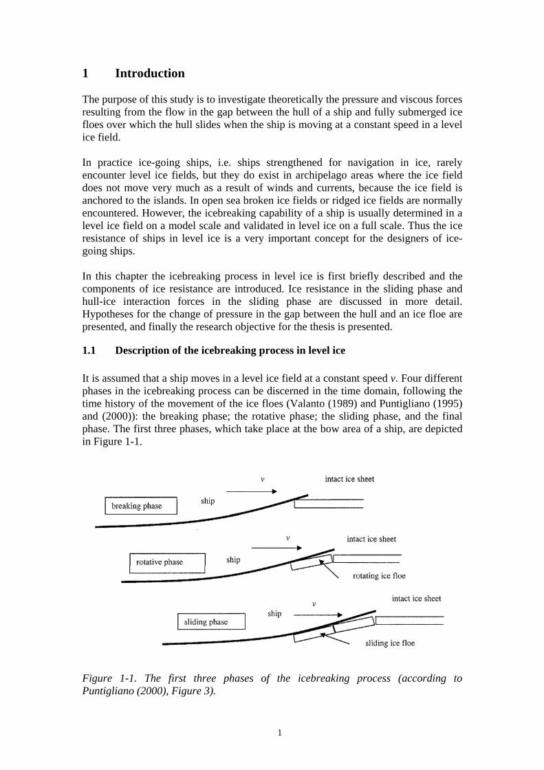
1.1 Description of the icebreaking process in level ice It is assumed that a ship moves in a level ice field at a constant speed v. Four different phases in the icebreaking process can be discerned in the time domain, following the time history of the movement of the ice floes (Valanto (1989) and Puntigliano (1995) and (2000)): the breaking phase; the rotative phase; the sliding phase, and the final phase. The first three phases, which take place at the bow area of a ship, are depicted in Figure 1-1.

Figure 1-1. The first three phases of the icebreaking process (according to Puntigliano (2000), Figure 3).

2

The breaking phase starts when the ship makes contact with the intact ice sheet and ends when a crack occurs, the intact ice sheet breaks, and a new ice floe is generated. During the rotative phase the bent ice floes are rotated until they are roughly parallel to the hull surface. During the icebreaking process the broken ice floes move mainly in a vertical direction under the hull of the ship, while the ship glides over them. During the sliding phase the ice floes will then be pushed further downwards along the hull and to a certain depth by other floes breaking after them, until they leave the hull. In the sliding phase the ice floes form a kind of "ice mat" below the forebody of the ship, consisting of irregularly shaped ice floes, as can be observed in Figure 1-2.

Figure 1-2. An underwater picture of a ship model advancing in thick level ice in the Wärtsilä Arctic Research Centre's (WARC) ice tank. The underwater hull surface is fully covered by ice floes (Valanto (2001a), Figure 4). During the final phase the ice floes move either beneath the lateral intact ice sheet by the sides of the ship or into the open channel in the wake of the ship, or the ice floes interact with the propeller(s) of the ship. 1.2 Definition of level ice resistance of a ship The ice resistance of a ship in level ice, iceR , is usually defined as ice tot owR R R= − (1.1) where totR is the total resistance of a ship in level ice and owR is the resistance of the ship in open water at the same speed (see for example Kashteljan and Ryvlin (1966) or Enkvist (1972)). Such a definition for level ice resistance may be considered to be

3

rather artificial, since the boundary conditions for fluid flow around the ship are quite different in ice and in open water. When the ship is moving in level ice, large areas of the hull are covered by ice, and the surrounding level ice cover may have a considerable effect on wave formation. This has been confirmed in the model tests of Leiviskä et al. (2001). Model tests in an ice-free channel which had a breadth about equal to the beam of the ship indicated that the resistance of the model in the ice-free channel was about twice the resistance of the model in open water. However, since the open water resistance of a ship is rather small compared with the ice resistance in the normal speed range used when navigating in ice (see Figure 1-3), the error resulting from the use of Equation (1.1) may not be very large.

0

200

400

600

800

1000

1200

1400

1600

0 2 4 6 8 10

v [m/s]

Res

ista

nce

[kN

] Resistance in open water

Ice resistance in level ice

Linear regression of the iceresistance data

Figure 1-3. Resistance of IB Vladivostok in open water and in 0.59 m thick level ice. Open water data is obtained from Kashteljan et al. (1973), Figure 73, and ice resistance data from Enkvist (1972), Figure 2.4.

1.3 Components of ice resistance in level ice The forces related to the ice-breaking and rotative phases in two dimensions have been studied in detail by Valanto (1989). Resistance components in level ice for three-dimensional hull shapes were studied by Valanto (2001a). Measured and computed resistance values and computed resistance components in level ice for Bay-class icebreakers are shown in Figure 1-4. Figure 1-4 shows the different resistance contributions from the numerically modelled physical processes at the waterline. The lowest curve shows the resistance resulting from the sliding phase, which is discussed in more detail in the next section. The distance between the lowest curve and the second curve with circles shows the resistance contribution resulting from ventilation during rotation of the ice floes from their original position to one tangential to the hull. Ventilation means that the ship is advancing so fast that the top surface of the rotating ice floe is wholly or partially free

4

of water during the rotative phase, even if the lower edge of the ice floe is located below the still water level. This phenomenon has been observed in nature when ships are advancing in level ice (Enkvist (1972)). It can be seen in Figure 1-4 that the contribution of ventilation to ice resistance is rather large and appears to vary little with speed. This is obviously caused by the fact that the length of the broken ice floes decreases as the speed of the ship increases (see Section 2.3). Valanto (1989) has studied the ventilation phenomenon for a two-dimensional hull form both by model tests and in theory, and in Valanto (2001a) theoretical calculations are presented for three-dimensional hull forms.

Figure 1-4. Measured and computed resistance values and computed resistance components in level ice for Bay-class icebreakers (Valanto (2001a), Figure 24). Fx is ice resistance, v is the speed of the ship, h is level ice thickness and s_f is the bending strength of level ice. The difference between the second curve (with circles) and the third curve (with triangles) shows the resistance contribution resulting from the rotating floes slamming against the hull at the end of the rotative phase. The difference between the third and fourth curves shows the resistance contribution caused by the ice floes breaking off the level ice field and accelerating to the speed dictated by the steady advance of the ship. These force peaks depend heavily on speed. The resistance contribution from ice being crushed at the bow is represented by the difference between the two uppermost curves. This contribution also depends on the speed of the ship. Two kinds of forces act at the contact points of the hull surface and ice, causing resistance to the motion of the ship: normal forces and tangential forces resulting from friction between the hull surface and the ice floes. In the ice-breaking phase the crushing of the ice edge and the bending and shearing of the ice edge into ice floes

5

cause these forces. In the rotative phase the acceleration of the broken ice floes and the water below the ice floes, the turning of the broken ice floes, and the inertia forces created when the turning ice floes strike against the hull surface cause normal and frictional forces between the hull and the ice floes. According to Figure 1-4, the increase of ice resistance with speed is mainly due to the increase in the resistance forces with speed in the ice-breaking phase and in the sliding phase. In this case the contribution of the resistance forces at the waterline level of the ship (the difference between the lowest and the uppermost curves in Figure 1-4) seems to be about half of the total resistance in level ice. The other half is caused by the sliding phase, i.e. the motion of the broken ice floes under the ship (the lowest curve in Figure 1-4). According to Puntigliano (2003, p. 2), ice resistance resulting from the sliding phase can be up to 65% of the total resistance of a ship advancing in level ice. 1.4 Ice resistance resulting from the sliding phase Valanto (2001a) used the empirical formula of Lindqvist (1989) to calculate the component of level ice resistance resulting from the sliding phase, which Lindqvist called submersion resistance (the lowest curve in Figure 1-4). According to Lindqvist, the total ice resistance resulting from the sliding phase, sR , can be calculated as the sum of the resistance resulting from the loss of the potential energy of the submerged ice floes and that resulting from friction acting between ice floes and the ship’s hull:

( )( )

2 2

/( 2 )

0.7 / tan 0.25 / tan

cos cos 1/ sin 1/ tan ],[

s ice

ice WL

R gh BT B T B T

gh B L T B

BT

ρ

μ ρ φ α

ψ φ φ α

Δ

Δ

= ⋅ + +

+ ⋅ ⋅ − −

+ +

(1.2)

where LWL is the waterline length, B the beam and T the draught of the ship, hice the level ice thickness, and α φ the waterline and the buttock angles of the bow, respectively, and ψ the angle between the normal to the bow and the vertical. ρΔ = ρw - ρice is the difference between the densities of water and ice, μ the friction coefficient, and g the acceleration of gravity. Formula (1.2) does not depend on the speed of the ship, v. Lindqvist recognised the need for more research in this area and used an empirical coefficient to describe the speed dependence as: ( ) ( )1 9.4 /s s WLR v R v gL= + , (1.3)

where Rs is according to (1.2). This formula indicates that the resistance of typical icebreakers in the sliding phase can increase to about three times the static value; see Valanto (2001a). It is unclear what the physical phenomena are that lie behind the increase in ice resistance with speed in the sliding phase given by Formula (1.3). In the following

6

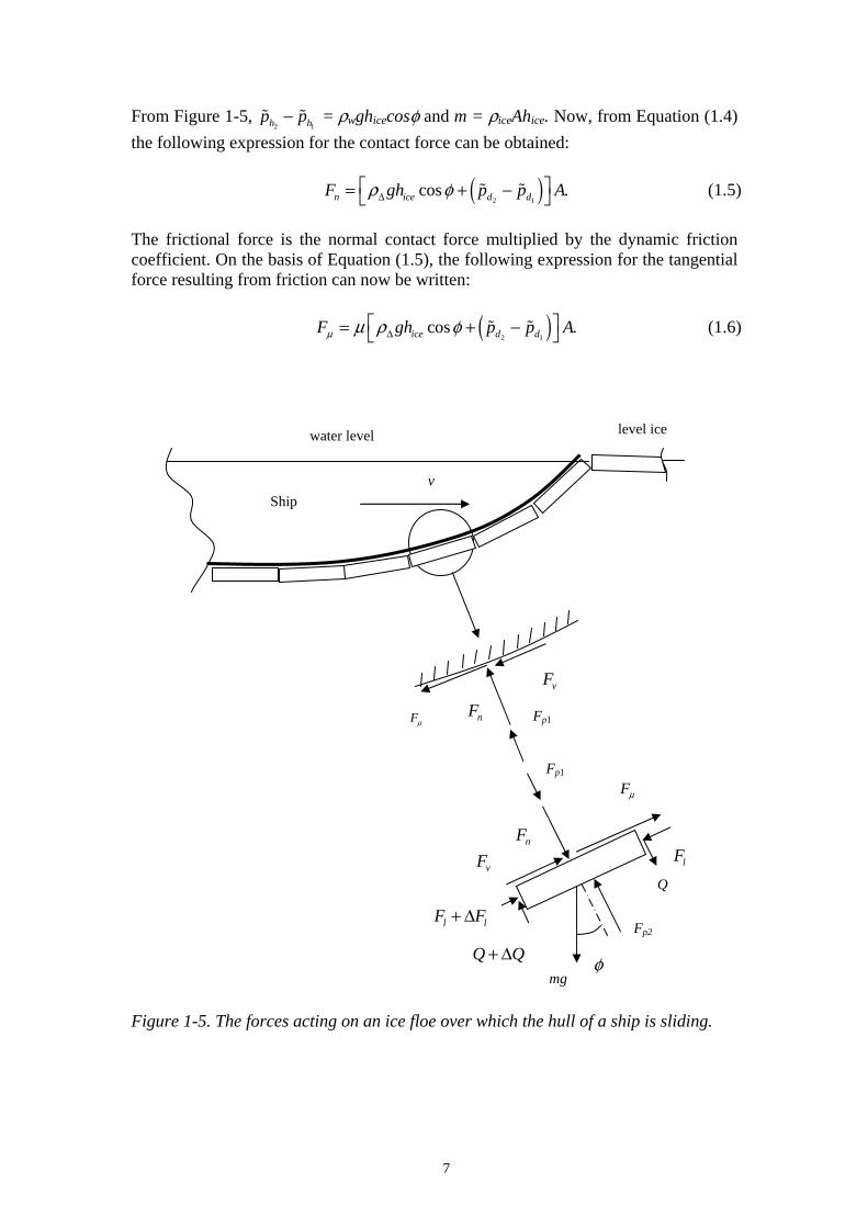
section the hull-ice interaction forces in the sliding phase will be considered in more detail. 1.5 Hull-ice interaction forces in the sliding phase For simplicity’s sake, the analysis is given for a two-dimensional hull form. In the sliding phase there may exist, in addition to the mechanical contact forces resulting from the static lift of the ice floes caused by the different densities of water and ice, two kinds of forces: forces resulting from changes in pressure in the gap between the hull surface and the ice floes or below the ice floe, and forces resulting from viscous shear stress caused by the flow of water in the gap. These forces may give rise to normal and frictional contact forces between the hull and the ice floes. If the hull of the ship has a positive (convex) curvature, an ice floe is in contact with the hull, in principle, at one location on the ice floe, as shown in Figure 1-5. At this location a normal force, Fn, acts perpendicular to the ice floe and the hull surface. Assuming the Coulomb friction law to be valid, the corresponding frictional force is nFμ , which causes the frictional resistance between the ice floe and the hull surface, μ being the friction coefficient. Fp1 is the force resulting from the pressure between the hull surface and the ice floe and Fp2 is the force resulting from the pressure below the ice floe. Fl denotes the sum of the tangential component of the contact force with the adjacent ice floe and the static pressure at the end surface of the ice floe, Q the shear force between the ice floe and the adjacent ice floe, Fv the tangential force caused by viscous stresses in the gap, m the mass of the ice floe, g the acceleration of gravity, and φ the angle between the tangent to the hull surface and horizontal at the contact point of the ice floe and the hull surface. Leaving out the forces acting at the edges of the ice floe, the equation of equilibrium normal to the ice surface, assuming that no inertia forces are acting in this direction, is, according to the free body diagram of the ice floe shown in Figure 1-5:

1 2cos 0.n p pF F F mg f+ - + = (1.4)

The pressure field above the ice floe is

1 11 h dp p p= + , where 1hp is static pressure and

1dp is the change in pressure or the so-called dynamic pressure (see Chapter 3). Now

1 1 1( )p h dF p p A= + is the force exerted by the pressure between the hull surface and

the ice floe, where ( )1 1/h hA

p p dA A= ∫ denotes the average hydrostatic pressure,

( )1 1/d dA

p p dA A= ∫ the average pressure change, and A the area of the ice floe.

Correspondingly, 2 22 h dp p p= + is the pressure field below the ice floe, where

2hp is static pressure and

2dp is the change in pressure. 2 2 2

( )p h dF p p A= + is the force

exerted by the pressure field below the ice floe, where ( )2 2/h hA

p p dA A= ∫ is the

average hydrostatic pressure below the ice floe and ( )2 2/d dA

p p dA A= ∫ is the average

pressure change.

7

From Figure 1-5, 2 1h hp p− = ρwghicecosφ and m = ρiceAhice. Now, from Equation (1.4)

the following expression for the contact force can be obtained: ( )2 1

cos .n ice d dF gh p p Ar fDÈ ˘= + -Î ˚ (1.5)

The frictional force is the normal contact force multiplied by the dynamic friction coefficient. On the basis of Equation (1.5), the following expression for the tangential force resulting from friction can now be written: ( )2 1

cos .ice d dF gh p p Am m r fDÈ ˘= + -Î ˚ (1.6)

Figure 1-5. The forces acting on an ice floe over which the hull of a ship is sliding.

Fp1 Fm

vF

nF

Ship v

water level level ice

Fp2

Fp1

Fm

mg φ

φ

nF

l lF F+ Δ

lF vF

Q Q+ Δ

Q

8

1.6 The effect of change in pressure below an ice floe on ice resistance in the sliding phase

It has been known for a long time that the displacement of water before the ship causes a change in the pressure field on the hull. Near the bow of the ship, the pressure is increased above the hydrostatic pressure, along the middle of the hull the pressure is decreased and at the stern it is again increased compared with the hydrostatic pressure below the hull of a motionless ship floating in still water. The ship sinks deeper when the magnitude of the negative dynamic pressure under the ship’s hull grows with the ship’s speed; this increases the hydrostatic pressure until the balance in vertical forces is reached. The trim of the ship may also change due to change in pressure below the ship’s hull (see, for example, van Manen and van Oossanen (1988)). The model tests conducted by Eggert (1939), showed that by integrating the longitudinal components of dynamic pressure forces over the length of the hull, the resulting resistance agreed fairly well with that measured on the model after the estimated frictional resistance had been subtracted. In other words, the pressure forces cause the so-called wave-making resistance. Enkvist (1972, page 130) conducted model tests with a model of the MV Jelppari to obtain an indication of the magnitude of the change in pressure below the bow of the model. The model was run in open water in order to record the distribution of pressure on its bow area. The results of the model tests of Enkvist (1972) are presented in Figure 1-6. It can be observed in this figure that in front of section 7 the pressure increases with increasing velocity of the model; behind section 7 the pressure decreases. In his analysis, Enkvist (1972) came to the conclusion that the measured pressure increase was too small to result in any significant increase of the resistance in level ice, assuming that the increase of resistance would be caused by additional frictional resistance caused by the increase of the pressure below the ice floes even if it is assumed that the broken ice field below the hull is assumed to be a continuous “ice mat”. Liukkonen (1989a) studied the same phenomenon computationally for a two-dimensional model using a Computational Fluid Dynamics (CFD) code. The velocity field and the distribution of pressure around the model were computed on the basis of the assumption that the ice field forms a watertight boundary around the ship model. He came to the same conclusion as Enkvist (1972) that the increase of level ice resistance with speed could not be explained by the change in pressure below the ice floes. However, Valanto (2001b) is of the opinion that below the layer of ice floes covering the hull there is a hydrodynamic pressure field which can press the ice floes against the hull with forces considerably higher than the buoyancy of the ice floes would cause. Puntigliano (2000) performed full-scale and model-scale tests in open water and in ice conditions with the MPV Neuwerk (see Section 2.2). He obtained similar type of results in his tests in open water for change in pressure in the bow area as Enkvist (1972) (see Figures 2-27 to 2-29). The question arising is that how good an approximation is the pressure distribution on the hull in open water for the pressure distribution below the ice floes, when the ship is advancing in level ice? Obviously the boundary conditions at the waterline level as

9

well as the submerged ice floes have a great influence on the pressure distribution below the ice floes. The model tests of Leiviskä et al. (2001) seem to indicate that the change in pressure below the hull is smaller in open water than in an ice channel. Thus the change in pressure below the ice floes when the ship is advancing in level ice would also be higher than the change in pressure below the hull in open water. On the other hand, the assumption that the ice field forms a watertight boundary around the ship when sailing in level ice, would probably overestimate the change in pressure below the ice floes.

Figure 1-6. The results of pressure measurements at the bow of the model of the MV Jelppari (Enkvist (1972), Appendix 8). Pressure measurements were made at the locations shown in the middle of the figure. The results of the pressure measurements at waterline 2 are shown on the lower part of the figure and the results at waterline 3 are shown on the upper part of the figure. Nevertheless, the data presented above indicates that the pressure below the ice floes changes with speed and also depends on the location of the ice floe in relation to the

10

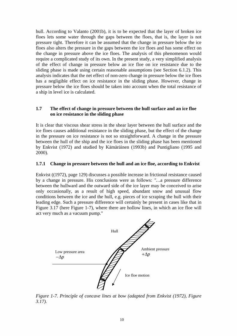
hull. According to Valanto (2001b), it is to be expected that the layer of broken ice floes lets some water through the gaps between the floes, that is, the layer is not pressure tight. Therefore it can be assumed that the change in pressure below the ice floes also alters the pressure in the gaps between the ice floes and has some effect on the change in pressure above the ice floes. The analysis of this phenomenon would require a complicated study of its own. In the present study, a very simplified analysis of the effect of change in pressure below an ice floe on ice resistance due to the sliding phase is made using certain reasonable assumptions (see Section 6.1.2). This analysis indicates that the net effect of non-zero change in pressure below the ice floes has a negligible effect on ice resistance in the sliding phase. However, change in pressure below the ice floes should be taken into account when the total resistance of a ship in level ice is calculated. 1.7 The effect of change in pressure between the hull surface and an ice floe

on ice resistance in the sliding phase It is clear that viscous shear stress in the shear layer between the hull surface and the ice floes causes additional resistance in the sliding phase, but the effect of the change in the pressure on ice resistance is not so straightforward. A change in the pressure between the hull of the ship and the ice floes in the sliding phase has been mentioned by Enkvist (1972) and studied by Kämäräinen (1993b) and Puntigliano (1995 and 2000). 1.7.1 Change in pressure between the hull and an ice floe, according to Enkvist Enkvist ((1972), page 129) discusses a possible increase in frictional resistance caused by a change in pressure. His conclusions were as follows: "…a pressure difference between the hullward and the outward side of the ice layer may be conceived to arise only occasionally, as a result of high speed, abundant snow and unusual flow conditions between the ice and the hull, e.g. pieces of ice scraping the hull with their leading edge. Such a pressure difference will certainly be present in cases like that in Figure 3.17 (here Figure 1-7), where there are hollow lines, in which an ice floe will act very much as a vacuum pump." Figure 1-7. Principle of concave lines at bow (adapted from Enkvist (1972), Figure 3.17).

Low pressure area p−Δ

Hull

Ice floe motion

Ambient pressure p+Δ

11

These conclusions can be understood to mean that a decrease in pressure may exist between the hull of a ship and an ice floe, in areas where there is a concave hull surface, as a result of restricted access of water into the gap between the hull and ice floes. Enkvist et al. (1979) state that during the rotative phase, a ventilated space is formed on top of the ice floe, which results in an essential increase in resistance. Valanto (2001b) is of the opinion that the ventilation phenomenon has an effect on the sliding phase as well, because ventilation may also cause a lack of water in the gap between the hull and the ice floes. This would explain the low-pressure phenomenon in the sliding phase. 1.7.2 Change in pressure between the hull and an ice floe, according to the author A new theory on pressure generation resulting from the flow of water in the gap between the hull of the ship and the ice floes was presented by the author in 1993. In Kämäräinen (1993b and 1994) it was assumed that there exists a flow of water induced by the relative motion of the hull surface of the ship with respect to the ice floes in the shear layer between the hull and the ice floes. A decrease in the pressure, increasing with the speed of the ship, can then occur in the shear layer in accordance with the Bernoulli equation and equation of continuity of the flow. The decrease in pressure along with speed in the shear layer will increase the contact forces between the hull and the ice floes. Thus ice resistance also increases along with speed as a result of increasing frictional forces between the hull surface and the ice floes. 1.7.3 Change in pressure between the hull and an ice floe, according to

Puntigliano Puntigliano (2000) has presented a mathematical model for the low-pressure phenomenon. According to Puntigliano, the phenomenon is the result of two phenomena: ventilation and the variation of the curvature of the hull during the sliding phase. The ventilation phenomenon is dominant at the beginning of the sliding phase, after the rotative phase, and the curvature variation increases its influence along the sliding trajectory of an ice floe. According to Puntigliano (2000), the pressure difference between the top and bottom of an ice floe is given by:

( ) ( )

2 21 1 ,

t b v w t w b

icew f w f

ice

p p c g T z g T z

hs c vR R h D

ρ ρ

ρ ρ

− = − − −

⎛ ⎞+ − + +⎜ ⎟+⎝ ⎠

(1.7)

where tp is the pressure on the top of an ice floe, bp is the pressure below an ice floe, vc is a correction factor related to the ventilation phenomenon, wρ is the density of water, g = 9.81 m/s2, T is the draught of the ship, tz is the vertical distance from the water level to the top of the ice floe, bz is the vertical distance from the water level to the bottom of the ice floe, s is the velocity of the ice floe (approximately equal to the speed of the ship, v), R is the local curvature of the hull surface at the

12

contact point of the hull and the ice floe, iceh is the ice thickness, fv is the velocity of the fluid through the gaps between the ice floe and the adjacent ice floes, D is an equivalent diameter of the gaps, and fc is a coefficient related to the viscous loss of pressure through the gaps. In Equation (1.7) the first term on the right-hand side is the hydrostatic component of the pressure between the ice and the hull. The second term is the hydrostatic pressure below the ice floe. The third term is related to the centrifugal force, which is slightly different on the top and bottom of the ice floe. The fourth term is related to the flux through the gaps between the ice floes. According to Puntigliano (2000), the first two terms and the last term are dominant. 1.7.4 The effect of change in pressure above an ice floe on ice resistance in the

sliding phase Three basic phenomena have been presented, which may cause a change in the pressure in the gap between the hull and an ice floe in the sliding phase:

- the ventilation phenomenon; - the acceleration of water in the shear layer in the gap between the ice floe and

the hull surface, and - the flow of water to and from the shear layer as a result of changes in the

geometry of the hull along the trajectory of an ice floe sliding against the hull. These phenomena have an effect on the change in pressure between the hull surface and the ice floe, but not below the ice floe. Assuming that the analysis made in Section 1.6 is valid, the change in pressure in the gap between the hull surface and an ice floe is

1 2 1

*d d dp p p= + , where

1

*dp is the possible change in pressure due to the last

two phenomena in the list given above. Equations (1.5) and (1.6) can now be written as follows:

1

*cos ,n ice dF gh p Ar fDÈ ˘= -Î ˚ (1.8) and

1

*cos ,ice dF gh p Am m r fDÈ ˘= -Î ˚ (1.9) where ( )1 1

* * /d dAp p dA A= ∫ is the average change in pressure due to the last two

phenomena given above. Thus, if the pressure between the hull surface and the ice floes decreases,

1

*dp is negative and the normal and the frictional forces between the

hull surface and the ice floe increase. 1.7.4.1 Normal and tangential forces acting on the hull The normal forces acting on the hull, Fnhull, resulting from the normal force between the hull and the ice floe and the average pressure change in the gap within the area of the ice floe, are: Fn given in Equation (1.8) and *

11

*

ddp

F p A= . Thus it can be written:

13

1 1

* *cos cos .nhull ice d d iceF gh p A p A gh Ar f r fD DÈ ˘= - + =Î ˚ (1.10) This means that:

The decrease in pressure in the gap between the hull and the ice floe may increase the resistance of a ship in level ice only through frictional forces given by Equation (1.9) - see Kämäräinen (1993b) - if the hull and the ice floe are in contact.

1.7.4.2 Ice resistance resulting from the sliding phase Ice resistance resulting from the sliding phase can now be calculated by using Equations (1.9) and (1.10), if the viscous forces are neglected. Assuming that the bow has a wedge-type form, i.e. a landing craft bow form, and considering the horizontal components of the forces, ice resistance resulting from the sliding phase is: ( )1

*sin cos cos ,s ice ice d fR gh gh p Ar f m r f fD DÈ ˘= + -Î ˚ (1.11)

where Af is the bow area of the ship. 1.8 The research objective Three basic phenomena have been presented which may cause a change in the pressure in the gap between the hull and an ice floe in the sliding phase:



geometry of the hull along the trajectory of an ice floe sliding against the hull. The research objective of this study was to study the effect of the last two phenomena on ice resistance in the sliding phase and to develop a calculation tool for this purpose. Before starting the theoretical consideration of the problem, model-scale test data on measured forces on the hull and pressure measurements on a model and on a full scale in the shear layer between the hull surface and ice floes are presented in Chapter 2. A definition of the calculation problem and an outline of the solution methods are presented in Chapter 3. In this study the Fluent and Iceflo CFD codes were used to calculate the flow between the hull surface and the ice floe. Fluent is a commercial CFD code and Iceflo is a CFD code developed for the purposes of this study. Fluent is presented in Chapter 4 and the theoretical basis of Iceflo in Chapter 5. The parameter studies of the calculation problem are introduced in Chapter 6. Discussion on the results of the calculations is presented in Chapter 7, a summary of the work is presented in Chapter 8, and conclusions are given in Chapter 9.

14

2 Model- and full-scale test data The use of segmented models in ice model tests provides an ideal way to measure ice resistance at different parts of the model. A number of tests of this kind have been carried out during the last two decades. Nawwar et al. (1984) had three horizontal sections near the waterline level in the bow area, Nyman (1986) had one horizontal section in the waterline area, Liukkonen (1989a) and Puntigliano (1995) cut the whole model into vertical sections in a transverse direction, and Liukkonen and Nortala-Hoikkanen (1992) and Kayo (1993) cut the model into both vertical and horizontal sections. Tests have also been carried out using pressure transducers to measure pressure in the shear layer between the ice floes and the hull (see Puntigliano (1995)). Izumiyama et al. (1999) have published results on pressure measurements using pressure sensors on the surface of the model. On a full scale, pressure measurements have been made using pressure transducers (see Puntigliano (2000)). In Section 2.1 those model tests and in Section 2.2 those full-scale tests which might give useful information on the forces acting on the hull in the sliding phase are briefly presented. Data on the size of ice floes on a full scale are presented in Section 2.3, examples of radii of the curvature of hull surfaces of ships are presented in Section 2.4, data on the surface roughness of the hull and ice surfaces are provided in Section 2.5, and a summary of Chapter 2 is presented in Section 2.6. 2.1 Model-scale test data 2.1.1 Model tests of Liukkonen with a two-dimensional model Liukkonen (1989a) conducted model tests with a segmented two-dimensional model to study the distribution of ice resistance in different parts of the hull. The model was divided into five vertical segments cut in a transverse direction, as shown in Figure 2-1. Vertical and longitudinal forces were measured separately from each segment. Between the segments there was a 3-5 mm wide gap where water could enter freely.

Figure 2-1. The segmented model used in the tests of Liukkonen. The dimensions given in the figure are in millimetres (Liukkonen (1989a), Figure 1). Vertical side plates 5000 mm in length and 700 mm in height were installed on both sides of the model in order to study the icebreaking phenomenon in two dimensions

15

(see Figure 2-2). A gap about 10 mm wide was left on both sides of the model between the model and the side plates. The model was not fixed to the towing carriage but was freely floating in water.

Figure 2-2. The arrangement of the side plates around the model (Liukkonen (1989a), Figure 3). The dimensions given in the figure are in millimetres.

0

1

2

3

4

5

6

7

8

0 0.1 0.2 0.3 0.4 0.5

Velocity [m/s]

Res

ista

nce

[N]

Total resistanceIce resistanceRegression lineResistance in open water

Figure 2-3. Measured total resistance, resistance in open water and ice resistance for Segment No. 2. Model ice thickness was 50 mm (data from Liukkonen (1989a), Table 2).

16

0

10

20

30

40

50

60

0 0.1 0.2 0.3 0.4 0.5

Velocity [m/s]

Forc

e [N

] Maximum normal forceRegression lineAverage normal forceRegression line

Figure 2-4. Measured maximum and average normal forces on Segment No. 2. Model ice thickness was 50 mm (data from Liukkonen (1989a), Table 3). A level ice strip with the same width as the model was sawn from a level ice field prior to the tests. The model was then towed along the ice strip so that the side plates ran in the longitudinal slots between the ice strip and the level ice field, and the model broke and displaced the level ice strip. In these tests a significant increase in ice resistance with speed was measured for Segment No. 2 (see Figure 2-3). An increase in ice resistance with speed was also observed for Segment No. 1, but the resistance measurements for the rest of the segments, Nos. 3 to 5, showed negligible dependence on speed. This was the first time that the increase in level ice resistance with speed in the sliding phase had been measured. However, the reason for this was not understood at that time (Liukkonen, 1989a). The maximum and average normal forces measured for Segment No. 2 are shown in Figure 2-4. In this figure it can be observed that the average normal force does not increase with speed, although the ice resistance, i.e. the longitudinal force, increases with speed. This observation is in line with the analysis of the influence of the pressure decrease phenomenon on the level ice resistance given in Section 1.7.4. 2.1.2 Model tests of Kayo with a segmented model Kayo (1993) performed ice model tests with a segmented bow model of an icebreaker. The body plan of the model is shown in Figure 2-5. The main dimensions of the model and model test parameters are given in Table 2-1.

17

Figure 2-5. Body plan of the model (Kayo (1993), Figure 1). Table 2-1. The main dimensions of the model and the model test parameters. The model scale factor, λ , was 25. Model Full-scale Lpp [m] 4.09 102.2 Bmax [m] 0.96 24.1 T [m] 0.42 10.5 Friction coefficient, μ 0.1 0.1 Ice thickness [m] 0.036

0.048 0.9 1.2

Flexular strength of the ice [kPa] 25 625 Model speed [m/s] 0.1-0.9 0.5-4.5

The bow of the model was divided into 21 panels (see Figure 2-6) and each panel was instrumented with a two-component load cell. As shown in Figure 2-6, only the fore part of the hull was used in the tests with the segmented model. Model tests with an intact model were also carried out in order to get a reference value for ice resistance. These tests were performed using the full model of the hull shown in Figure 2-5.

Figure 2-6. Test arrangement and segmentation of the partial model (Kayo (1993), Figures 4 and 5).

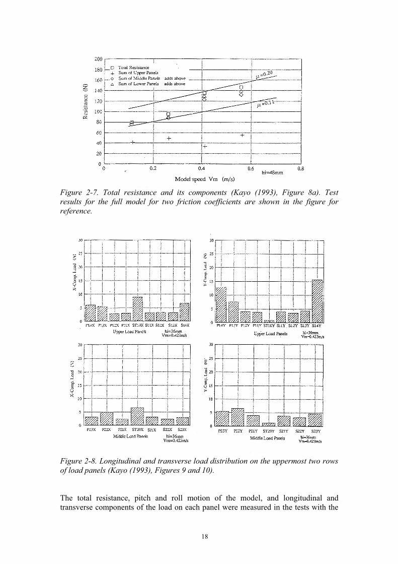
18

Figure 2-7. Total resistance and its components (Kayo (1993), Figure 8a). Test results for the full model for two friction coefficients are shown in the figure for reference.

Figure 2-8. Longitudinal and transverse load distribution on the uppermost two rows of load panels (Kayo (1993), Figures 9 and 10). The total resistance, pitch and roll motion of the model, and longitudinal and transverse components of the load on each panel were measured in the tests with the

19

segmented model. An example of the longitudinal component of the mean load of the load panels is shown in Figure 2-7. The loads observed on the middle panels, P2x and S2x, are considerably higher than those of P3x and S3x of the lower panels, as well as those of P1x and S1x of the upper panels. The load on the middle panels seems to increase considerably with speed, whereas the load on the upper panels increases only moderately with speed. The vertical dimensions of the panels are not given in Kayo (1993) nor the size of the broken ice floes, but presumably the ice-breaking and rotative phases take place mainly in the area of the upper panels and the ice-sliding phase on the second and the third rows of panels. These measurements thus also indicate a strong increase in ice resistance with speed in the sliding phase. A more detailed distribution of the longitudinal and transverse forces on the two uppermost rows of load panels is shown in Figure 2-8. In this figure high longitudinal forces at the stem and high transverse loads can be observed in the shoulder areas of the model on the first row of panels at the waterline. A much more uniform distribution of the longitudinal and transverse load components can be observed on the second row of panels. 2.1.3 Model tests of Puntigliano with a simplified Waas Bow Puntigliano (1995) presented the results of a series of model tests where the physical phenomena contributing to resistance under the design waterline were investigated. A segmented model of a simplified Waas Bow type was used in the tests. The main dimensions of the model are shown in Table 2-2. The hull form is shown in Figure 2-9 and the general arrangement of the instrumentation of the bow of the model is shown in Figure 2-10. Table 2-2. Principal dimensions of the model (Puntigliano (1995), Table 1). Lpp is the length of the model, B is the beam of the model, T is the draught of the model, D is the side height of the model, and φ is the bow angle with horizontal at the construction water line of the model. Model

(scale 1:20) Full-scale

Lpp [m] 5.0 100.0 B [m] 1.0 20.0 T [m] 0.35 7.0 D [m] 0.6 12.0 φ [deg] 16.5 16.5

The model was provided with three segments on the port side, two windows on the bottom at the starboard side, which permitted direct observation of the flow between the ice and the hull, and built-in pressure transducers under the bottom on the starboard side. Gaps of 4 mm in width were left between the segments. Differential pressure transducers and water column manometers were used to measure the pressure between the ice floes and the hull surface of the model.

20

Figure 2-9. Line drawing of the simplified Waas bow (Puntigliano (2003), Fig. 2).

Figure 2-10. General arrangement of the simplified Waas Bow. The segments with their load cells (e.g. F11X) can be seen on the port side and the pressure transducers (pt) on the starboard side (Puntigliano (1995), Figure 31). Model tests were carried out using three ice thicknesses (40 mm, 50 mm, and 70 mm, corresponding to 0.8 m, 1.0 m, and 1.4 m on a full scale) and five speeds (0.2 m/s, 0.4 m/s, 0.6 m/s, 0.8 m/s, and 1.0 m/s, corresponding to 1.74 kn, 3.48 kn, 5.22 kn, 6.96 kn, and 8.7 kn on a full scale), using level ice and different types of pre-sawn ice. In the model tests all degrees of freedom of the model except the translational movement were restrained. The model tests revealed an important low pressure area in the forebody (see Figure 2-11). The difference between the pressure on the top and under the bottom of the floes was estimated by approximating the pressure under the submerged ice cover

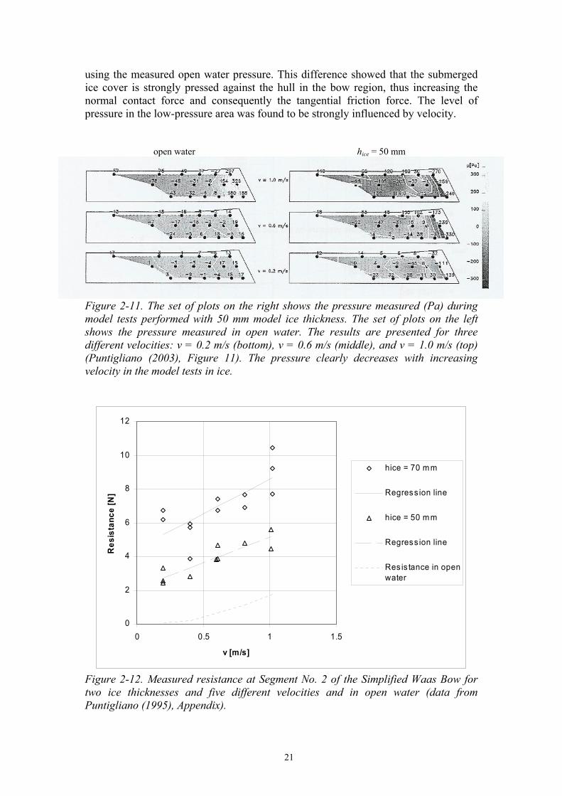
21

using the measured open water pressure. This difference showed that the submerged ice cover is strongly pressed against the hull in the bow region, thus increasing the normal contact force and consequently the tangential friction force. The level of pressure in the low-pressure area was found to be strongly influenced by velocity. open water hice = 50 mm

Figure 2-11. The set of plots on the right shows the pressure measured (Pa) during model tests performed with 50 mm model ice thickness. The set of plots on the left shows the pressure measured in open water. The results are presented for three different velocities: v = 0.2 m/s (bottom), v = 0.6 m/s (middle), and v = 1.0 m/s (top) (Puntigliano (2003), Figure 11). The pressure clearly decreases with increasing velocity in the model tests in ice.

0

2

4

6

8

10

12

0 0.5 1 1.5

v [m/s]

Res

ista

nce

[N]

hice = 70 m m

Regress ion line

hice = 50 m m

Regress ion line

Res is tance in openwater

Figure 2-12. Measured resistance at Segment No. 2 of the Simplified Waas Bow for two ice thicknesses and five different velocities and in open water (data from Puntigliano (1995), Appendix).

22

The total normal force on the hull was found to be independent of the pressure on the top of the ice floes and consequently not to contribute more to resistance than the open water and the hydrostatic buoyancy of ice do (Puntigliano (1997)). The tangential force was found to be the main contributor to resistance under the design waterline and it increased very considerably with increasing velocity (see Figure 2-12). These observations are in line with the analysis of the influence of the pressure decrease phenomenon on level ice resistance given in Section 1.7.4. Measured vertical force at Segment No. 2 is depicted in Figure 2-13 for two ice thicknesses. With increasing velocity the total vertical force at Segment No. 2 clearly decreases. According to Puntigliano (1997) one possible reason for this phenomenon is that the hydrodynamic pressure field below the submerged ice floes decreases with increasing velocity.

0

5

10

15

20

25

30

0 0.2 0.4 0.6 0.8 1 1.2

v [m/s]

Vert

ical

forc

e [N

]

hice = 70 mmRegression linehice = 50 mmRegression line

Figure 2-13. Measured vertical force at Segment No. 2 of the Simplified Waas Bow for two ice thicknesses and five different velocities (data from Puntigliano (1995), Appendix). The results of the pressure measurements in open water and in ice are compared in Figures 2-14 to 2-16. The results of the pressure measurements on the centreline (Transducers Nos. 1, 4, 7, 10, and 13) are given in Figure 2-14. The results of the pressure measurements for the transducers located at B/4 are shown in Figure 2-15 (Transducers Nos. 2, 5, 8, 11, and 14) and those at the side of the model (Transducers Nos. 3, 6, 9, 12, 15, and 18) in Figure 2-16. The bow of the ship is located at the right-hand side of the figures. In these figures it can be seen that in open water there is high pressure in the bow area because of the bow wave. In contrast, in ice conditions low pressure in the same area as a result of ventilation can be observed.

23

h ice = 50 mm, v = 1 m/s Transducers at the CL

-0.3

-0.2

-0.1

0

0.1

0.2

0.3

1 1.2 1.4 1.6 1.8 2 2.2 2.4

x [m]

Pres

sure

[kPa

]

In open waterIn ice

Figure 2-14. Results of the pressure measurements for the transducers at the CL. Data from Puntigliano (2003), Appendix A.2, Table 19.

h ice = 50 mm, v = 1 m/s Transducers at B /4

-0.3-0.2-0.1

00.10.20.30.4

1 1.2 1.4 1.6 1.8 2 2.2 2.4

x [m]

Pres

sure

[kPa

]

In open waterIn ice

Figure 2-15. Results of the pressure measurements for the transducers at B/4. Data from Puntigliano (2003), Appendix A.2, Table 19.

h ice = 50 mm, v = 1 m/s Transducers at side

-0.3

-0.2

-0.1

0

0.1

0.2

0.3

1 1.2 1.4 1.6 1.8 2 2.2 2.4

x [m]

Pres

sure

[kPa

]

In open waterIn ice

Figure 2-16. Results of the pressure measurements for the transducers at the side. Data from Puntigliano (2003), Appendix A.2, Table 19.

24

2.1.4 Model tests of Puntigliano with a cylindrical bow Puntigliano (1995) also presented the results of a series of ice model tests where a segmented model with a bow in the form of an inclined cylinder was used. The main dimensions of the model are shown in Table 2-3. Table 2-3. Principal dimensions of the model with the cylindrical bow. Model

(scale 1:20) Full-scale

Lpp [m] 5.0 100.0 B [m] 1.0 20.0 T [m] 0.35 7.0 D [m] 0.6 12.0 φ [deg] 16.5 16.5

Figure 2-17. A line plan of the cylindrical bow model (Puntigliano (1995), Figure 114).

Figure 2-18. The general arrangement of the model showing the segments, load cells (e.g. F11X), and pressure transducers (pt) (Puntigliano (1995), Figure 122).

25

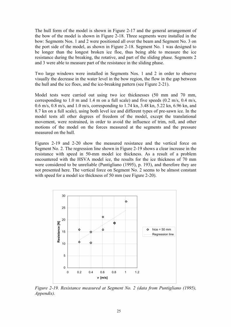
The hull form of the model is shown in Figure 2-17 and the general arrangement of the bow of the model is shown in Figure 2-18. Three segments were installed in the bow: Segments Nos. 1 and 2 were positioned all over the beam and Segment No. 3 on the port side of the model, as shown in Figure 2-18. Segment No. 1 was designed to be longer than the longest broken ice floe, thus being able to measure the ice resistance during the breaking, the rotative, and part of the sliding phase. Segments 2 and 3 were able to measure part of the resistance in the sliding phase. Two large windows were installed in Segments Nos. 1 and 2 in order to observe visually the decrease in the water level in the bow region, the flow in the gap between the hull and the ice floes, and the ice-breaking pattern (see Figure 2-21). Model tests were carried out using two ice thicknesses (50 mm and 70 mm, corresponding to 1.0 m and 1.4 m on a full scale) and five speeds (0.2 m/s, 0.4 m/s, 0.6 m/s, 0.8 m/s, and 1.0 m/s, corresponding to 1.74 kn, 3.48 kn, 5.22 kn, 6.96 kn, and 8.7 kn on a full scale), using both level ice and different types of pre-sawn ice. In the model tests all other degrees of freedom of the model, except the translational movement, were restrained, in order to avoid the influence of trim, roll, and other motions of the model on the forces measured at the segments and the pressure measured on the hull. Figures 2-19 and 2-20 show the measured resistance and the vertical force on Segment No. 2. The regression line shown in Figure 2-19 shows a clear increase in the resistance with speed in 50-mm model ice thickness. As a result of a problem encountered with the HSVA model ice, the results for the ice thickness of 70 mm were considered to be unreliable (Puntigliano (1995), p. 193), and therefore they are not presented here. The vertical force on Segment No. 2 seems to be almost constant with speed for a model ice thickness of 50 mm (see Figure 2-20).

0

5

10

15

20

25

30

0 0.2 0.4 0.6 0.8 1 1.2

v [m/s]

Res

ista

nce

[N]

hice = 50 mmRegression line

Figure 2-19. Resistance measured at Segment No. 2 (data from Puntigliano (1995), Appendix).

26

0

5

10

15

20

25

30

35

0 0.2 0.4 0.6 0.8 1 1.2

v [m/s]

Vert

ical

forc

e [N

]

hice = 50 mmRegression line

Figure 2-20. Vertical force measured at Segment No. 2 (data from Puntigliano (1995), Appendix).

Figure 2-21. Inside view through the window at Segment No. 2, v = 0.4 m/s, hice = 50 mm (Puntigliano (1995), Figure 169). Ten pressure transducers were installed in three rows on Segments Nos. 1 and 2, as shown in Figure 2-18. The first row of pressure transducers was installed on the centreline of the model, the second row at a distance of 0.2 m from the centreline, and the third row at a distance of 0.4 m from the centreline. According to Puntigliano (2003) the results of the model tests concerning the pressure measurements were found to be inaccurate and the scatter of the measurements was high. However, the

27

experiments with the cylindrical bow model were good enough to demonstrate the existence of a low pressure field at the bow area.

Figure 2-22. Water level, ZWL, observed in the cylindrical bow model (hice = 50 mm). The draught of the model was at z = 0.35 m (top of the diagram) (Puntigliano (1995), Figure 167). An example of the breaking pattern is shown in Figure 2-21. During the model tests, the water level between the hull and ice was observed visually through the built-in windows. The water level was found to oscillate as a result of the icebreaking cycle in the ice-breaking phase. In Figure 2-22 data on the observed average water level are given. This figure clearly shows the ventilation phenomenon, which was almost exclusively limited to the area of Segment No. 1, never reaching the waterline z = 0.24 m. Below this level a mixture of small air bubbles and small ice pieces was observed flowing between the hull and the ice. The velocity of the small ice pieces was at the highest model velocity (1.0 m/s), approximately half of the model velocity. This indicates that there is probably a shear driven Couette-type flow in the gap (see e.g. Figure 4-1 in Chapter 4). However, at lower velocities the air bubbles and small ice pieces mainly accompanied the model (Puntigliano (1995), p. 228). 2.1.5 Model tests on hull-ice contact In resistance tests at the ice tank of the Ship Research Institute of Japan for a model of the PM Teshio1, a new type of pressure sensor was used to measure local ice loads on the model hull (Izumiyama et al. (1999)). Local ice loads were measured along the waterline of the model from the stem to Section No. 6.5 (see Figure 2-23). The main dimensions of the model were: LOA = 5.051 m, B = 0.973 m, and T = 0.303 m.

1 An ice-breaking patrol ship of the Maritime Safety Agency of Japan

28

With the tactile sensor system it was possible to make pressure measurements with a very high spatial resolution. The sensors were thin flexible films of a size 240 mm by 240 mm, with a thickness of about 0.3 mm. On the film there were sensing spots in a grid-like arrangement of 44 rows by 44 columns. The spacing between the sensing spots was about 5.4 mm. The sensors could only measure positive pressure, i.e. over-pressure.

Figure 2-23. Locations of the sensor films (Izumiyama et al. (1999), Figure 2). Figure 2-24 shows an example of the data obtained by the tactile sensor system. The figure shows a typical pattern of model-ice contact in level ice at a model speed of 0.779 m/s. Model ice thickness was 41 mm. Figures 2-24 (a)-(g) are frames which show pressure distribution on a sensor film at Location No. 3 (see Figure 2-23). The waterline of the model is at the top of the frames and the left-hand side of the frames is the bow side. Figure 2-24(h) shows the time history of the sum of the data over the film for a time period of 0.7 s. According to Izumiyama et al. (1999), the process shown in Figure 2-24 consists of two different phases in terms of the contact of the model with the ice and ice load. The first phase lasts from the point in time 0.05 s to 0.5 s in Figure 2.24(h). Four frames of this phase are shown in Figures 2-24(a)-(d). The second phase takes place after the point in time 0.5 s, and three frames for this phase are shown in Figures 2-24(e)-(g). In the first phase it can be seen that relatively high pressure is acting over a narrow area, as shown in Figures 2-24(a)-(d). The pressured areas are distributed so that they form a line. The line moves downwards and disappears at the time point 0.5 s. In the second phase relatively low pressure acts over a wider area. The pressure area moves upwards in this phase as time passes. The total load shows another peak at the time point 0.6 s. It seems that Figures 2-24(a)-(d) show a typical line-like contact of the broken ice edge and the model hull during the rotative phase. However, the contact shown in Figures 2-24(e)-(g) seems to be different from that in the first phase. According to Izumiyama the type of loading shown in these figures was caused by impact of the ice floe against the hull surface in the end of the rotative phase. This would also explain the fact that the loaded area moves upwards on the surface of the model when the time passes. It can also be observed that the contact of the ice floe or floes with the model surface takes place at a finite number of spots. This indicates that the ice surface may be uneven. However, it may well be that these figures show the loading of an ice floe

29

which slides against the model surface and at the same time slightly rotates, because the ice floe having caused the loading shown in Figures 2-24(a)-(d), may have passed Sensor No. 3, when the load measurements shown in Figures 2-24(e)-(g) were made. It is difficult to draw final conclusions on the reason of the type of loading shown in these figures, because information of the size of the broken ice floes is not available and the icebreaking process at the waterline level was not video taped (personal correspondence with Izumiyama, 2006).

Figure 2-24. Example of measured ice load (Izumiyama et al. (1999), Figure 4).

30

2.2 Full-scale and model-scale test data with MPV Neuwerk 2.2.1 Full-scale test data In 1999 full-scale tests were carried out with the MPV Neuwerk in the northern Baltic Sea. Seven pressure transducers were installed on the ship, as shown in Figure 2-25, to measure the low-pressure phenomenon (Puntigliano (2000)). Measurements were made in open water and in level ice. The low-pressure phenomenon was measured on a full scale for the first time on March 5th, 1999 at 21:15 hours.

Figure 2-25. Positions of the pressure transducers installed on the MPV Neuwerk (Puntigliano (2003), Figure 18).

Figure 2-26. At t = 4270 s Neuwerk enters level ice. The measured pressure drops continuously from 7.5 to -7.5 kPa at t =4440 s and the velocity of the ship drops to about 1 kn. At t = 4530 s the ship stopped (Puntigliano (2000), Figure 16).

31

The ship was advancing in an open ice channel through Storfjärden in Ångmansälven when she entered level ice with a thick snow cover. Figure 2-26 shows the time history of the measured pressure. As shown in the figure, the measured pressure drops by about 11 kPa after the ship had entered level ice. Meanwhile the velocity decayed to approximately 1.7 kn.

Figure 2-27. Pressure measured at Pressure Transducer No. 3. The influence of the snow thickness (hs) and equivalent ice thickness (he) are presented on the left- and right-hand sides respectively (Puntigliano (2000), Figure 19).

Figure 2-28. Pressure measured at Pressure Transducer No. 5. The influence of the snow thickness (hs) and equivalent ice thickness (he) are presented on the left- and right-hand sides respectively (Puntigliano (2003), Figure 28).

32

The pressure measured at Pressure Transducer No. 3 is shown in Figure 2-27. Similar data were obtained for Pressure Transducers Nos. 1 to 4. These transducers were located quite near the waterline and thus the decrease in the water head with speed may be explained by the ventilation phenomenon. The pressure measurements at Pressure Transducer No. 5 are shown in Figure 2-28. This pressure transducer was located deep below the waterline and thus the decrease in pressure with speed cannot be explained by ventilation. It is interesting to observe that the open water tests showed no change in pressure at this location irrespective of the velocity of the model. This phenomenon may be understood when comparing these results with the pressure measurements performed by Enkvist (1972), see Figure 1-6. The location of Pressure Transducer No. 5 in the longitudinal direction shown in Figure 2-25 is quite similar to the location of the two pressure transducers at section 7 in Figure 1-6. Pressure Transducer No. 7 showed no decrease in pressure with speed. Because of the location of that transducer, it was estimated by HSVA that this transducer may not have encountered ice at all. 2.2.2 Model-scale test data A set of model tests was performed to measure the pressure field between ice and the hull of the MPV Neuwerk (Puntigliano (2003)). The aim of the tests was to compare the measured values with the results obtained in the full-scale trials performed in the Gulf of Bothnia. The model scale used was λ = 14.286.

Figure 2-29. Pressure measured during the model tests at the same positions where the pressure transducers were installed for the full-scale tests (Puntigliano (2003), Figure 16).

33

Figure 2-29 shows the results obtained in the model tests at the same measuring points as in the full-scale tests. The measurements show high scatter, but the low-pressure phenomenon can be recognised. 2.3 Data on the size of ice floes on a full scale As already pointed out by Enkvist (1972), the size of the broken ice floes is an important parameter affecting the resistance of ships in level ice. In Figure 2-30 the depth of broken lens-type ice floes is depicted according to full-scale tests carried out with a small tug, the Jelppari. The ship has a traditional icebreaking bow form. The level ice thickness ranged from 0.14 m to 0.25 m. In this figure it can be seen that the scatter of cusp depth is high, but it also clearly shows that the cusp depth, i.e. the size of the broken ice floes, decreases as the speed of the ship increases. Valanto (1993) presents data on the length of the broken ice floes for the icebreaker Kapitan Sorokin with a Thyssen/Waas bow form. The measurements were made during the full-scale trials of the ship carried out on the Yenisei river estuary in May 1991. An example of the results is given in Figure 2-31, which shows the length of the broken ice floes versus the speed of the ship. The ice thickness was about 1.8 m, covered with 0.25 m to 0.4 m of snow. In Figure 2-31 the same tendency as in the tests with the Jelppari can be recognised: at low speed the scatter of the measured length of the broken ice floes is high, but at higher speeds the scatter decreases. The length of the broken ice floes also decreases with speed.

Figure 2-30. Depth of broken cusps, l, with respect to the speed of the ship, vs, according to full scale-tests with the Jelppari (Enkvist (1972), Figure 2.10).

34

0

1

2

3

4

5

6

7

0 0.5 1 1.5 2 2.5 3 3.5 4 4.5

Speed of the ship [m/s]

Leng

th o

f the

ice

floe

[m]

Figure 2-31. Length of the broken ice floes versus the speed of the ship on May 12-13, 1991 (according to Valanto (1993), Table 3). 2.4 Radii of curvature of real hull surfaces A number of hull forms of ice-going ships are available to study the curvature of the real hull surfaces of ice-going ships (see e.g. Kämäräinen (1993a)). The results of the analysis of two ships, the IB Kapitan Evdokimov and IB Taimyr, are presented here. It was assumed that the diagonals of the fore parts of the hulls shown in Figures 2-32 and 2-33 roughly represent the path of an ice floe below the fore part of the ship during the sliding phase. A diagonal is a curve drawn along the section points of the frames and the diagonal plane. The curvature of a diagonal was calculated in the x1-coordinate direction as follows:

2121

3/ 221

1

1

1

i

i

ii

x

i

d ydx

R dydx

= −⎡ ⎤⎛ ⎞⎢ ⎥+ ⎜ ⎟⎢ ⎥⎝ ⎠⎣ ⎦

, (2.1)

where

ixR is the radius of the curvature of the diagonal in Section i and 1iy is the

breadth of the diagonal in Section i. The radius of the curvature was calculated numerically from Equation (2.1) using the finite difference method. For the sake of simplicity it was assumed that the radius of the diagonal represents the radius of the curvature of the hull surface in the longitudinal direction and the radius of the curvature of the construction frames represents the radius of the curvature of the hull surface in the transverse direction of the path of the ice floe. The radius of the curvature of the frames, Ry, was calculated at the planes of the frames in the same way

35

as the radius of the curvature of the diagonal. The radius of the curvature of the diagonals, Rx, and the frames, Ry, of the above-mentioned ships are presented in Figures 2-34 and 2-35. z1 x1

y1

Figure 2-32. The bow construction frames of the Kapitan Evdokimov (Zuev (1986)).

Figure 2-33. The bow and stern construction frames of the IB Taimyr (Tsoy and Sinjajev (1989)).

0

20

40

60

80

100

120

140

160

18036.5 46.5 56.5 66.5 76.5

x [m] from AP

Rxor

Ry [m

]

Rx of EvdokimovRy of Evdokimov

Figure 2-34. The approximated radii of the curvature, Rx and Ry, of the hull surface of the IB Kapitan Evdokimov.

y1

36

0

50

100

150

200

250

300

350

40070.4 80.4 90.4 100.4 110.4 120.4 130.4 140.4 150.4

x [m] form AP

Rx

or R

y [m

]

Rx of TaimyrRy of Taimyr

Figure 2-35. The approximated radii of the curvature, Rx and Ry, of the hull surface of the IB Taimyr. In Figure 2-34 it can be seen that both radii of curvature of the hull surface of the IB Kapitan Evdokimov decrease from mid ship to stem. The same applies for the IB Taimyr, but forward from about 100 m from the aft perpendicular, the radii of curvature start to increase slightly in magnitude (see Figure 2-35). 2.5 Surface roughness of the hull and ice surfaces The surface roughness of a surface is defined in the standard SFS-EN ISO 4287 (1999) as follows:

0

1 ( )l

aR Z x dxl

= ∫ , (2.2)

where Ra is the centreline average of the surface roughness, l is the measuring length, and Z(x) is the height of the surface from the centreline. The centreline average can also be calculated as a mean of the distances between the centreline and the surface; see Figure 2-36.

1

1 n

a ii

R Zn =

≈ ∑ (2.3)

In Table 2-4 some values of the centreline average of surface roughness, Ra, are given for hull and ice surfaces. Liukkonen (1992) gives values of the surface roughness for hull and ship model coatings.

37

Figure 2-36. The profile of the surface. Table 2-4. Centreline average, Ra, values of the surface roughness for different coatings and natural ice without snow cover. Coating Ra [ mμ ] Source Inerta 160 (ship coating) 20 Liukkonen (1992), Table 1 Interlux 709 + Intermix (model coating)

1.5 Liukkonen (1992), Table 1

Natural ice 690 Johansson (1988), p. 24

Figure 2-37. Surface height profile, histogram, and corrected histogram for natural sea ice (Johansson (1988), Figure 5.11).

Z1 Z2

z

x

38

Johansson (1988) used an 850-nm laser to collect one-dimensional surface profiles of both snow and ice during the BEPERS-88 experiment. The measurements were made in the Gulf of Bothnia in March 1988. Natural ice without snow cover was found in a ship channel where the ice had developed in calm water. Figure 2-37 shows one of the measured profiles. Johansson (1988) showed that the surface roughness of the ice surface can be assumed to be Gaussian-distributed. The transparency of the natural ice caused some measurement errors, which can be seen in the numerous spikes of the profile and in the histogram, which is tailed in the negative direction. A corrected histogram is also presented in Figure 2-37. The mean value of the surface height standard deviation, σ , after the spikes outside the 99.9% confidence interval had been eliminated, was less than a millimetre. This value shows how extremely smooth the ice surface can be (Johansson (1988), page 23). 2.6 Summary of Chapter 2 All the model-scale data presented above indicate that there exists an increase in ice resistance with speed in the sliding phase. The model tests of Liukkonen (1989a) for a two-dimensional model indicate that the normal forces do not increase with speed in the sliding phase, although the ice resistance does increase with speed in the sliding phase. The model tests of Puntigliano (1995 and 2003), both for a two-dimensional model and a cylindrical bow model, even indicate that the normal forces decrease with speed in the sliding phase, although the ice resistance does increase with speed in the sliding phase. These observations, together with the measurements of low pressure in the boundary layer between the hull surface and the ice floes, both on a model scale (Puntigliano (1995 and 2003)) and on a full scale (Puntigliano (2000 and 2003)), strongly support the idea that the increase in ice resistance in the sliding phase is due to either the increase in the mechanical friction forces or viscous forces between the hull surface and the ice floes, or both. The model test data of Izumiyama et al. (1999) indicate that the contact between the hull surface and the ice floes takes place at a finite number of spots. Thus there may be some room for water to flow in the shear layer between the hull surface and the ice floes. A flow in the gap between the hull and the ice floes was observed in the model tests of the cylindrical bow form (Puntigliano (1995)). The measurements made by Enkvist (1972) and Valanto (1993) indicate that the length of the broken ice floes decreases when the speed of the ship increases. The broken ice floes are also larger in thick level ice than in thin level ice. In the next chapter the numerical tools needed to calculate the pressure and viscous forces in the gap between the hull surface and the ice floes are considered.

39

3 Definition of the calculation problem and outline of the solution methods

In this chapter the governing equations, i.e. the Navier-Stokes equations, are given in Section 3.1 and the calculation problem is presented in Section 3.2. In Section 3.2 the reduced Navier-Stokes equations based on the hydrodynamic lubrication theory are also presented. An outline of the solution methods for the shear-driven motion of a fluid between the hull surface and an ice floe in relative motion is presented in Section 3.3.

3.1 The governing equations It is a generally accepted fact that the motion of a Newtonian fluid is governed by the Navier-Stokes equations, irrespective of whether the flow is laminar, transitional, or turbulent. The full Navier-Stokes equations, or conservation of momentum equations, in an inertial (non-accelerating) reference frame under gravity body forces can be written in Cartesian tensor form by (see e.g. Paterson (1997), p. 132):

( ) ( ) 2 3

ji ki j i i

j i j j i i k

uu upu u u g Kt x x x x x x xr r r h h

È ˘Ê ˆ∂ È ˘∂ ∂∂ ∂ ∂ ∂ ∂ Ê ˆ+ = - + + + -Í ˙ Í ˙Á ˜Á ˜ Ë ¯∂ ∂ ∂ ∂ ∂ ∂ ∂ ∂Ë ¯Í ˙ Î ˚Î ˚ (3.1)

where t is the time, r the density of the fluid, iu the velocity component in the ix -coordinate direction, ig the acceleration of gravity in the ix -coordinate direction, p the pressure, h the molecular viscosity, and K the second coefficient of viscosity. The equation of conservation of mass, or the continuity equation, can be written in Cartesian tensor form by:

( ) 0ii

ut xr r∂ ∂+ =∂ ∂

. (3.2)

In the following analysis it is assumed that the density and viscosity of the fluid are constants. If the pressure in the gap between the hull surface and a fully submerged ice floe is considered, the pressure p in Equation (3.1) may be defined as consisting of hydrostatic pressure, ph, measured from the water level and dynamic pressure, pd

: h dp p p= + . (3.3) In Section 1.5 p1 denoted the pressure in the gap between the hull surface and an ice floe,

1hp static pressure and 1dp dynamic pressure, but from now on, for the sake of

simplicity, these quantities are written without subscript “1”. If the zero level of the static pressure is set as a vacuum, atmospheric pressure should be added to the right-hand side of Equation (3.3). This is relevant if flow film cavitation is considered (see Section 5.2.5). When there is no fluid motion in the gap, the dynamic pressure is zero and Equation (3.1) reduces to:

40

hi

i

pgx

ρ ∂=∂

(3.4)

Inserting Equations (3.3) and (3.4) into Equation (3.1) and taking the constancy of ρ into account in (3.1) and (3.2), the following simplified equations for the conservation of momentum and mass are obtained (see e.g. Paterson (1997), pp. 134-135):

( )2

i d ij i

j i j j

u p uu u

t x x x xr r h∂ ∂ ∂∂+ = - +∂ ∂ ∂ ∂ ∂

(3.5)

0i

i

ux

∂ =∂

(3.6)

In Cartesian coordinates Equations (3.5) and (3.6) can be written as follows:

( ) ( ) ( )

( ) ( ) ( )

( ) ( ) ( )

2 2 2

2 2 2

2 2 2

2 2 2

2 2 2

2 2 2

d

d

d

pu u u uuu uv uwt x y z x x y z

pv v v vuv vv vwt x y z y x y z

pw w w wuw vw wwt x y z z x y z

r h

r h

r h

Ê ˆÈ ˘ ∂∂ ∂ ∂ ∂ ∂ ∂ ∂+ + + = - + + +Í ˙ Á ˜∂ ∂ ∂ ∂ ∂ ∂ ∂ ∂Ë ¯Î ˚Ê ˆÈ ˘ ∂∂ ∂ ∂ ∂ ∂ ∂ ∂+ + + = - + + +Í ˙ Á ˜∂ ∂ ∂ ∂ ∂ ∂ ∂ ∂Ë ¯Î ˚Ê ˆÈ ˘ ∂∂ ∂ ∂ ∂ ∂ ∂ ∂+ + + = - + + +Í ˙ Á ˜∂ ∂ ∂ ∂ ∂ ∂ ∂ ∂Ë ¯Î ˚

(3.7)

0u v wx y z

∂ ∂ ∂+ + =∂ ∂ ∂

, (3.8)

where u, v, and w are the velocity components of the flow in the x-, y-, and z-coordinate directions. There are now four equations, (3.7) and (3.8), for the four unknowns u, v, w, and pd. The solution of the above equations becomes fully determined physically when the boundary and initial conditions are specified. If needed, the total pressure, p, can be obtained by just adding the hydrostatic pressure, ph, to the dynamic pressure, pd ; see Equation (3.3). However, in this thesis the effect of fluid motion on the pressure in the gap between the hull surface and the ice floes is the main subject of the study and, therefore, when reference is made to "pressure" in the following chapters, this means the "dynamic pressure", dp , unless otherwise stated. 3.1.1 Turbulence modelling The most advanced method for solving Equations (3.5) and (3.6) would be to use a Direct Numerical Simulation (DNS) method. This means that the whole turbulent flow field is solved numerically using the Navier-Stokes equations. No semi-empirical turbulence models are used and the result is a three-dimensional, time-dependent flow field which includes all scales of motion down to the Kolmogorov length scale.

41

However, a complete time-dependent solution of the exact Navier-Stokes equations for high-Reynolds-number turbulent flows in complex geometries is unlikely to be attainable for some time to come because of the huge amount of computer resources required. Two alternative methods can be employed to transform the Navier-Stokes equations in such a way that the small-scale turbulent fluctuations do not have to be directly simulated: "Reynolds averaging" and "filtering". Both methods introduce additional terms in the governing equations that need to be modelled in order to achieve "closure", i.e. to have a sufficient number of equations for all the unknowns. The Reynolds-averaged approach is generally adopted for practical engineering calculations, and uses semi-empirical models such as one-equation models, like the Spalart-Allmaras model, two-equation models, such as the k e- model and its variants, and the Reynolds Stress Model (RSM). Large Eddy Simulation (LES) provides an alternative approach in which the large eddies in a turbulent flow are computed in a time-dependent simulation that uses a set of "filtered" equations. Filtering is essentially a manipulation of the exact Navier-Stokes equations to remove only those eddies that are smaller than the size of the filter, which is usually taken as the mesh size. However, the application of LES to industrial fluid simulation is still in its infancy (Fluent (1998), p. 9-4). Therefore the author decided to concentrate the computational efforts on the Reynolds-averaged approach, which is described in more detail in the following section. 3.1.2 Reynolds averaging In Reynolds averaging, the solution variables in the instantaneous (exact) momentum and continuity equations (3.5) and (3.6) are decomposed into mean (ensemble-averaged or time-averaged) and fluctuating components. For the velocity components: '

i i iu u u= + (3.9) where ' and i iu u are the mean and fluctuating velocity components. Likewise, for the pressure it can be written: '

d d dp p p= + (3.10) where ' and d dp p are the mean and fluctuating components of the pressure. Substituting expressions of this form for the flow variables into the instantaneous momentum and continuity equations (3.5) and (3.6) and taking a time (or ensemble) average yields the time-averaged continuity and momentum equations:

( ) ( )2' 'i d i

j i j ij i j j j

u p uu u u u

t x x x x xr r h r∂ ∂ ∂∂ ∂+ = - + -∂ ∂ ∂ ∂ ∂ ∂

(3.11)

42

0i

i

ux∂ =∂

(3.12)

Equations (3.11) and (3.12) are called the "Reynolds-averaged" Navier-Stokes (RANS) equations. They have the same general form as the instantaneous Navier-Stokes equations, but the velocities and other solution variables now represent time-averaged values. Additional terms now appear that represent the effects of turbulence. These "Reynolds stresses", ' '

i ju ur- , must be modelled in order to close Equation (3.11). A common method employs the Boussinesq hypothesis to relate the Reynolds stresses to the mean velocity gradients (see e.g. Ferziger and Peric (2002), p. 294):

' ' 23

jii j t ij

j i

uuu u k

x xr h rd

Ê ˆ∂∂- = + -Á ˜∂ ∂Ë ¯

(3.13)

where th is turbulent viscosity, k turbulent kinetic energy, and ijδ the Kronecker delta symbol. Turbulence kinetic energy k can be calculated using the following equation, which can be obtained from Equation (3.13) by making j equal to i:

' '12 i ik u u= , (3.14)

The advantage of the Boussinesq approach is the relatively low computational effort associated with the computation of the turbulent viscosity, th . The disadvantage of this hypothesis is that it assumes turbulent viscosity, th , to be an isotropic scalar quantity, which is not strictly true. 3.2 Analysis of the calculation problem As was discussed in Section 1.1, during the icebreaking process the broken ice floes move mainly in a vertical direction under the hull of the ship when the ship is gliding over them (see Figure 3-1). In Figure 3-1 it can be seen that when the ship advances a distance l at a velocity v, the relative motion between the hull and an ice floe is also approximately the speed of the ship, v. It is assumed that the hull has a convex, “egg-shaped” hull form and consequently there is one point or a small area where an individual ice floe is in contact with the hull surface. The aim is to develop a numerical calculation method to determine the steady or unsteady shear-driven flow velocity and pressure fields in a converging-diverging gap between the hull surface and a rectangular ice floe, as shown in Figure 3-2. The upper drawing in Figure 3-2 depicts the gap between a rectangular ice floe and a convex hull form. The origin is placed in the middle of the contact area of the hull surface and the ice floe. The gap has a height, h, which is a function of x and y. The length and breadth of the ice floe are l and b. The hull surface has a radius of curvature, Rx, in the x-coordinate direction and Ry in the y-coordinate direction. The hull surface moves at a speed, U, in the positive x-axis direction and the speed of the ice floe is assumed to be zero. The hull surface is thus the driving surface for the shear-driven flow in the gap between the two surfaces. The hull surface and the surface of the ice floe are

43

assumed to be perfectly smooth. The fluid in the gap is assumed to be water at a constant temperature with constant density and viscosity. Figure 3-1. Kinematics of the ice-submerging process. Figure 3-2. The geometry considered in the thesis.

v

l

Hull of the ship

Water level

Section A - A

Upper surface of the ice floe

Hull surface z

x u=0

u=U

l

h

y

Rx

Ry z

x h(x,y)

y

A A

Hull surface

Ice floe l

b

U

44

The lower drawing in Figure 3-2 depicts a section, A-A, of the gap between the ice floe and the hull surface. A flow is generated in the gap as a result of the motion of the hull surface. On the surface of the ice floe the flow has a speed of zero and on the hull surface the flow speed equals the speed of the hull surface as a result of the no-slip boundary conditions on the solid surfaces. The flow field and the pressure in the gap depend on the boundary conditions at the edges of the ice floe. The problem is further simplified by assuming that the tangential velocity of the hull surface equals U, since the radius of the hull surface, Rx, is much larger than the length of the ice floe, l. The length scale of the film in the (x,y) plane of Figure 3-2 is l and h is the length scale across the thickness of the gap. For typical lubricant films (Szeri (1998), p. 71): ( )3( / ) 10h l O −= . (3.15) As an example, it is now assumed that the hull has a spherical shape, 75xR = m,

75yR = m, and the ice floe has a rectangular shape with dimensions l x b = 2 m x

2 m. The fluid in the gap is assumed to be water at 0oC with a density 31000 kg/mρ = and a viscosity 0.001792 Pa sη = ⋅ . In this example the gap height varies from 0 to 6.7 mm and thus h/l varies from 0 to 33.4 10−⋅ m. This indicates that the order of magnitude of the various terms in the governing equations (3.7) and (3.8) can be evaluated in a similar way as for fluid film bearings (see Szeri (1998), Chapter 2.2). The variables participating in the Navier-Stokes equations are first normalised, assuming that b l∼ , by defining: ˆ ˆ ˆ/ , / , / ,x x l y y l z z h= = = (3.16) giving the non-dimensional coordinates ˆ ˆ ˆ, and x y z , which range from 0 to 1. Similarly, the velocity is normalised by using the maximum velocity, U, in the x,y-plane: ˆ ˆ ˆ/ , / , / ,u u U v v U w w W= = = (3.17) where W is the velocity scale in the direction across the film:

.hW Ul

⎛ ⎞= ⎜ ⎟⎝ ⎠

(3.18)

The non-dimensional quantities for pressure, ˆˆ , and time, ,dp t are defined as:

2

2 ˆˆ Re , dd C

ph Up t tl U lρ

⎛ ⎞= =⎜ ⎟⎝ ⎠

. (3.19)

ReC is the local Couette Reynolds number:

45

Re2CUh

ν= , (3.20)

where ν is the kinematic viscosity of the fluid, /ν η ρ= . The non-dimensionalised forms of Navier-Stokes equations can now be written by inserting Equations (3.16), (3.17), and (3.18) into the Navier-Stokes equations (3.7) and (3.8), and taking account of Equations (3.19):

( ) ( ) ( )

( ) ( ) ( )

22 2 2*

2 2 2

22 2 2*

2 2 2

2

ˆˆ ˆ ˆ ˆ2ˆ ˆ ˆ ˆ ˆ ˆReˆ ˆ ˆ ˆ ˆ ˆˆ ˆ

ˆˆ ˆ ˆ ˆ2ˆ ˆ ˆ ˆ ˆ ˆReˆ ˆ ˆ ˆ ˆ ˆˆ ˆ

2R

d

d

pu u u h u uuu uv uw

t x y z x z l x y

pv v h v vuv vv vw

t x y z y z l x y

hl

∂∂ ∂ ∂ ∂ ∂ ∂ ∂+ + + = - + + +

∂ ∂ ∂ ∂ ∂ ∂ ∂ ∂

∂∂ ∂ ∂ ∂ ∂ ∂ ∂+ + + = - + + +

∂ ∂ ∂ ∂ ∂ ∂ ∂ ∂

Ê ˆÈ ˘ Ê ˆÁ ˜Í ˙ Á ˜Ë ¯ Ë ¯Î ˚

Ê ˆÈ ˘ Ê ˆÁ ˜Í ˙ Á ˜Ë ¯ Ë ¯Î ˚

Ê ˆÁ ˜Ë ¯ ( ) ( ) ( )

22 2 2*

2 2 2

ˆ ˆ ˆ ˆ2ˆ ˆ ˆ ˆ ˆ ˆeˆ ˆ ˆ ˆ ˆˆ ˆ

w w h w wuw vw ww

t x y z z l x y∂ ∂ ∂ ∂ ∂ ∂ ∂

+ + + - - + =∂ ∂ ∂ ∂ ∂ ∂ ∂

Ï ¸Ê ˆÈ ˘ Ê ˆÌ ˝Á ˜Í ˙ Á ˜Ë ¯ Ë ¯Ô Î ˚ ÔÓ ˛

ˆ

ˆdp

z∂

-∂

(3.21)

ˆ ˆ ˆ

0ˆ ˆ ˆu v wx y z

∂ ∂ ∂+ + =

∂ ∂ ∂. (3.22)

Here the reduced Reynolds number, Re*, is defined as follows:

2Re* ReChl

⎛ ⎞= ⎜ ⎟⎝ ⎠

. (3.23)

As was earlier noted, the length scale ( ) ( )3/ 10h l O −= , and therefore the last equation in (3.21), can be completely dispensed with, as:

( )6ˆ10 ,

ˆdp Oz

−∂ =∂

(3.24)

Thus, to order (h/l)2, the pressure is constant across the film: ( )ˆˆ ˆ ˆ ˆ, ,d dp p x y t= . The first two equations in (3.21) now show that inertia terms will survive if

( )Re* 1O≥ . On taking the limit ( )2/ 0h l → in the equations in (3.21) the reduced Navier-Stokes equations in non-dimensional form can be obtained:

( ) ( ) ( )

( ) ( ) ( )

2*

2

2*

2

ˆˆ ˆˆ ˆ ˆ ˆ ˆ ˆRe ˆ ˆ ˆ ˆˆ ˆ

ˆˆ ˆˆ ˆ ˆ ˆ ˆ ˆRe ˆ ˆ ˆ ˆˆ ˆ

d

d

pu uuu uv uwt x y z x z

pv vuv vv vwt x y z y z

È ˘ ∂∂ ∂ ∂ ∂ ∂+ + + = - +Í ˙∂ ∂ ∂ ∂ ∂ ∂Î ˚È ˘ ∂∂ ∂ ∂ ∂ ∂+ + + = - +Í ˙∂ ∂ ∂ ∂ ∂ ∂Î ˚

(3.25)

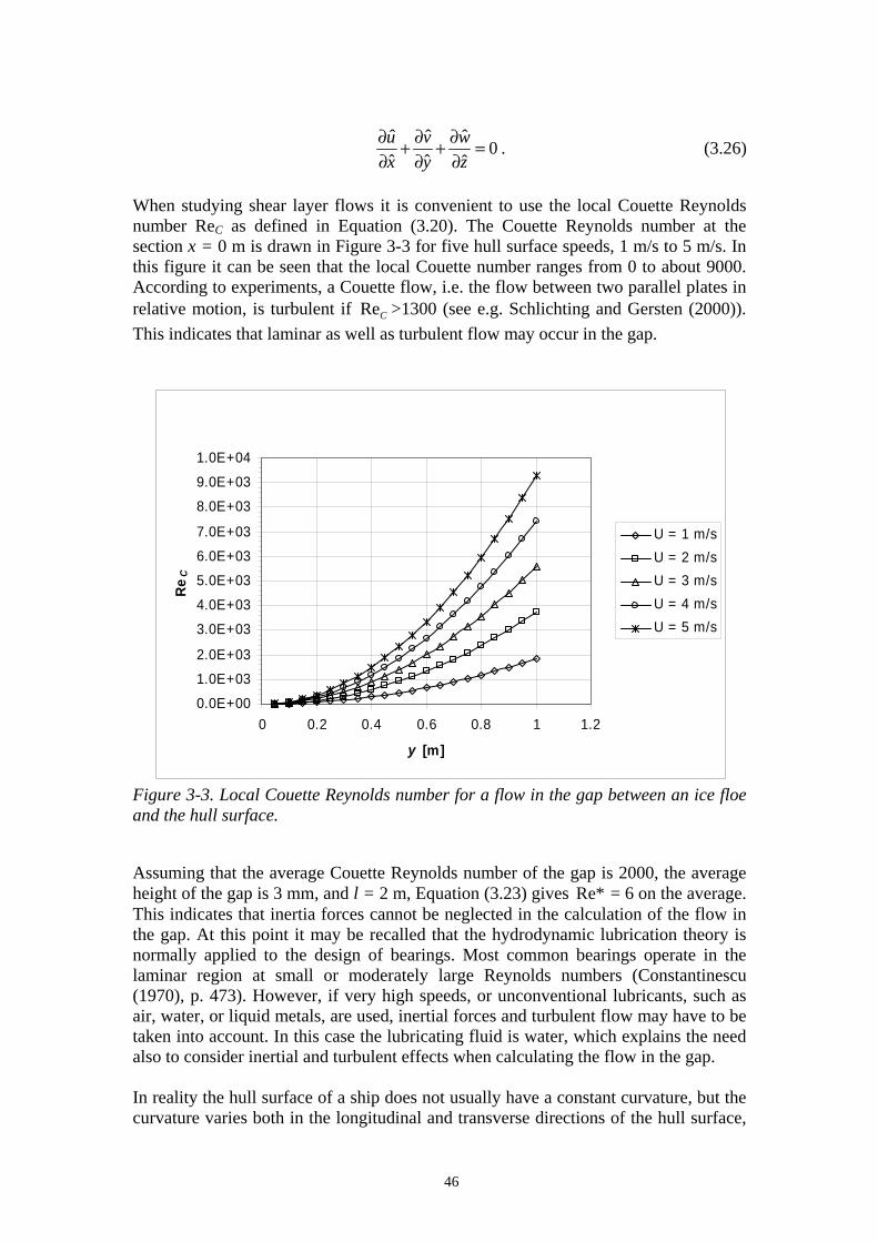
46

ˆ ˆ ˆ

0ˆ ˆ ˆu v wx y z

∂ ∂ ∂+ + =∂ ∂ ∂

. (3.26)

When studying shear layer flows it is convenient to use the local Couette Reynolds number ReC as defined in Equation (3.20). The Couette Reynolds number at the section x = 0 m is drawn in Figure 3-3 for five hull surface speeds, 1 m/s to 5 m/s. In this figure it can be seen that the local Couette number ranges from 0 to about 9000. According to experiments, a Couette flow, i.e. the flow between two parallel plates in relative motion, is turbulent if ReC >1300 (see e.g. Schlichting and Gersten (2000)). This indicates that laminar as well as turbulent flow may occur in the gap.

0.0E+00

1.0E+03

2.0E+03

3.0E+03

4.0E+03

5.0E+03

6.0E+03

7.0E+03

8.0E+03

9.0E+03

1.0E+04

0 0.2 0.4 0.6 0.8 1 1.2

y [m]

ReC

U = 1 m/sU = 2 m/sU = 3 m/sU = 4 m/sU = 5 m/s

Figure 3-3. Local Couette Reynolds number for a flow in the gap between an ice floe and the hull surface. Assuming that the average Couette Reynolds number of the gap is 2000, the average height of the gap is 3 mm, and l = 2 m, Equation (3.23) gives Re* = 6 on the average. This indicates that inertia forces cannot be neglected in the calculation of the flow in the gap. At this point it may be recalled that the hydrodynamic lubrication theory is normally applied to the design of bearings. Most common bearings operate in the laminar region at small or moderately large Reynolds numbers (Constantinescu (1970), p. 473). However, if very high speeds, or unconventional lubricants, such as air, water, or liquid metals, are used, inertial forces and turbulent flow may have to be taken into account. In this case the lubricating fluid is water, which explains the need also to consider inertial and turbulent effects when calculating the flow in the gap. In reality the hull surface of a ship does not usually have a constant curvature, but the curvature varies both in the longitudinal and transverse directions of the hull surface,

47

as can be seen in the examples given in Figures 2-32 and 2-33. This indicates that the flow in the gap is not stationary, but time-dependent. The preliminary analysis of the flow in the gap, based on the calculation of the Couette Reynolds number and the reduced Reynolds number for the example case, thus indicates that the calculation method has to be able to model time-dependent laminar and turbulent shear flows with inertia effects in the gap between the hull surface and an ice floe. The method must also be able to model contact between the surfaces at a certain point or area within the gap. 3.3 Outline of the solution methods Two strategies now exist to solve the calculation problem described in the previous section. Attempts can be made to solve either the "full" Navier-Stokes equations (3.5) and (3.6) or the simplified Navier-Stokes equations (3.25) and (3.26). In general, the problem of finding exact analytical solutions to the Navier-Stokes equations (3.5) and (3.6) presents insurmountable mathematical difficulties. Nevertheless, it is possible to find exact solutions in certain particular cases with simple geometry, mostly when the quadratic convective terms vanish in a natural way (Schlichting (1979), p. 83). In general, numerical methods have to be used to solve the full or simplified Navier-Stokes equations. The most commonly used methods are the finite difference method, the finite volume method, and the finite element method. Hybrid methods also exist, combining, for example, the finite volume and the finite element methods. One can clearly see that the numerical solution of the simplified Navier-Stokes equations can be obtained much more easily than the solution of the full Navier-Stokes equations, since the simplified equations have one equation less to be solved than the full Navier-Stokes equations. Therefore the analyses in this thesis are mainly performed by solving the simplified equations. For this purpose the Iceflo computer code was developed (see Chapter 5), which is based on the finite difference method. However, for reference, some calculations were performed by solving the full Navier-Stokes equations. These calculations were carried out by the commercial CFD computer code Fluent, which is based on the finite volume method. Some aspects of the Fluent computer code are described in the next chapter.

48

4 The Fluent computational fluid dynamics computer code In this chapter some aspects of the Fluent CFD computer code are described in Section 4.1. In order to evaluate the suitability of Fluent for the analysis of the computational problem described in the previous chapter, Fluent is validated in Section 4.2 against the direct numerical simulation (DNS) data of Bech et al. (2000) for plane-turbulent Couette flow, and against the experimental data of Nakabayashi (1993) for a turbulent Couette-type flow with repeated longitudinal pressure gradients. The Fluent computer code was installed on CSC's2 SGI Origin 2000 platform cedar.csc.fi. Preprocessing was carried out using Gambit, which is part of the Fluent package. After preprocessing, the CFD solver of Fluent does the calculations and produces the results. Post-processing can also be performed by Fluent. 4.1 The Fluent CFD computer code Although Finite Element methods have recently gained popularity in the field of CFD applications, most of the commercial CFD software, like Fluent, is still based on the Finite Volume (FV) method. The finite volume method uses the integral form of the conservation equation as the starting point. For example, the momentum conservation inside an arbitrary control volume V can be expressed as (see e.g. Blazek (2001), p. 10):

( ) ( )d d deV S V S S

udV u u n S f dV pn S n St

ρ ρ ρ τ∂ + ⋅ = − + ⋅∂ ∫ ∫ ∫ ∫ ∫ , (4.1)

where u is the fluid velocity, V the volume occupied by the control volume, S the surface enclosing the control volume, n the unit vector orthogonal to S and directed outwards, efρ the body force per unit volume, and τ stands for the viscous stress tensor. A benefit of writing the governing equation in this particular form is that the conservation laws are fulfilled implicitly. More detailed information on the finite volume method and its numerical implementation can be found in the literature, such as Patankar (1980), Anderson et al. (1984), and Ferziger and Peric (2002). The following turbulence models can be used in Fluent: - Standard k e- model - Standard k ω− model - Spalart-Almaras turbulence model - Low Reynolds number k e- model - RNG k e- model - Realisable k e- model

2 CSC is the Finnish IT centre for science, administered by the Ministry of Education of Finland

49

As an example of the turbulence models of Fluent, the standard k e- model as given in Fluent (1998) is described in Section 4.1.1. Descriptions of the other turbulence models mentioned above can be found in Fluent (1998). 4.1.1 The Standard k ε− turbulence model used by Fluent The standard k ε− model (see e.g. Launder and Spalding (1972)) is a semi-empirical model based on model transport equations for the turbulent kinetic energy, k, and its dissipation rate, e . The model transport equation for k is derived from Navier-Stokes equations, while the model transport equation for e is obtained using physical reasoning and bears little resemblance to its mathematically exact counterpart. In the derivation of the k e- model, it is assumed that the flow is fully turbulent and the effects of molecular viscosity are negligible. The standard k e- model is therefore valid only for fully turbulent flows. 4.1.1.1 Transport equations for the standard k ε− model The turbulent kinetic energy, k, and its rate of dissipation, e , are obtained from the following transport equations:

tk b M

i k i

Dk k G G YDt x x

hr h res

È ˘Ê ˆ∂ ∂= + + + - -Í ˙Á ˜∂ ∂Ë ¯Í ˙Î ˚ (4.2)

and

( )2

1 3 2t

k bi i

D C G C G CDt x x k ke e e

e

he e e er h rs

È ˘Ê ˆ∂ ∂= + + + -Í ˙Á ˜∂ ∂Ë ¯Í ˙Î ˚ (4.3)

In these equations, kG represents the generation of turbulent kinetic energy resulting from the mean velocity gradients, bG is the generation of turbulent kinetic energy caused by buoyancy, and MY represents the contribution of the fluctuating dilatation in compressible turbulence to the overall dissipation rate. 1 2 3, and C C Ce e e are constants.

and k es s are the turbulent Prandtl numbers for k and e , respectively. 4.1.1.2 Modelling turbulent production in the k ε− model From the exact equation for the transport of k, the term kG , representing the production of turbulent kinetic energy, may be defined as:

' ' jk i j

i

uG u u

xr

∂= -

∂. (4.4)

kG is evaluated in a manner consistent with the Boussinesq hypothesis:

50

2

k tG Sh= , (4.5) where S is the modulus of the mean rate-of-strain tensor, defined as: 2 ij ijS S S∫ , (4.6) with the mean strain rate ijS given by:

12

jiij

j i

uuSx x

Ê ˆ∂∂= +Á ˜∂ ∂Ë ¯

. (4.7)

4.1.1.3 Modelling the turbulent viscosity The "eddy'' or turbulent viscosity, th , is computed by combining k and e as follows:

2

tkCmh re

= , (4.8)

where Cm is a constant. 4.1.1.4 Model constants The model constants 1 2, , , , and kC C Ce e m es s have the following default values (see Launder and Sharma (1974)):

1 21.44, 1.92, 0.09, 1.0, and 1.3kC C Ce e m es s= = = = = These default values have been determined from experiments with air and water for fundamental turbulent shear flows, including homogeneous shear flows and decaying isotropic grid turbulence. They have been found to work fairly well for a wide range of wall-bounded and free shear flows. 4.2 Validation of Fluent In this section the turbulence models of Fluent are validated against the direct numerical simulation data of Bech et al. (1995 and 2000) for plane-turbulent Couette flow, which are considered the most consistent and readily available data for this type of flow (Bech et al. (1995), p. 299). The calculation results of Fluent are also compared with the experimental data of Nakabayashi (1993) for a turbulent Couette-type flow with repeated longitudinal pressure gradients.

51

4.2.1 Validation of the turbulence models of Fluent Bech et al. (1995 and 2000) studied the turbulence structure in plane Couette flow at low Reynolds numbers using data obtained both from direct numerical simulation and physical experiments. The plane turbulent Couette flow studied by Bech et al. (1995 and 2000) is depicted in Figure 4-1. Figure 4-1. Schematic illustration of plane-turbulent Couette flow. The upper wall was moving at a speed of 2U with respect to the lower wall, which was stationary. The half-channel height, h, was 0.01 m. The fluid between the plates was water. The properties of the fluid were not given in Bech et al. (1995 and 2000). The Fluent standard values for water were used ( 20 oT C= ) in the calculations: ρ = 998.2 kg/m3 and η = 0.001003 Pa s⋅ . The Couette Reynolds number was Re / 1300Uh n= = (Bech et al. (1995), p. 303, and (2000)) from which the speed of the upper wall, 2 0.261 m/sU = , can be obtained. Using the notation of Bech et al. (1995), the Couette Reynolds number as defined in Equation (3.20) is Re 2 /C Uh n= . This means that in the experiments the Couette Reynolds number, as defined in this thesis, was 2600 and thus the flow was turbulent (see Section 3.2). The friction velocity uτ is defined as:

wuttr

= , (4.9)

where wt is the wall shear stress. Bech et al. (1995) define the Reynolds number on the basis of wall friction velocity,

z

x

2U

2h

Moving wall

Stationary wall

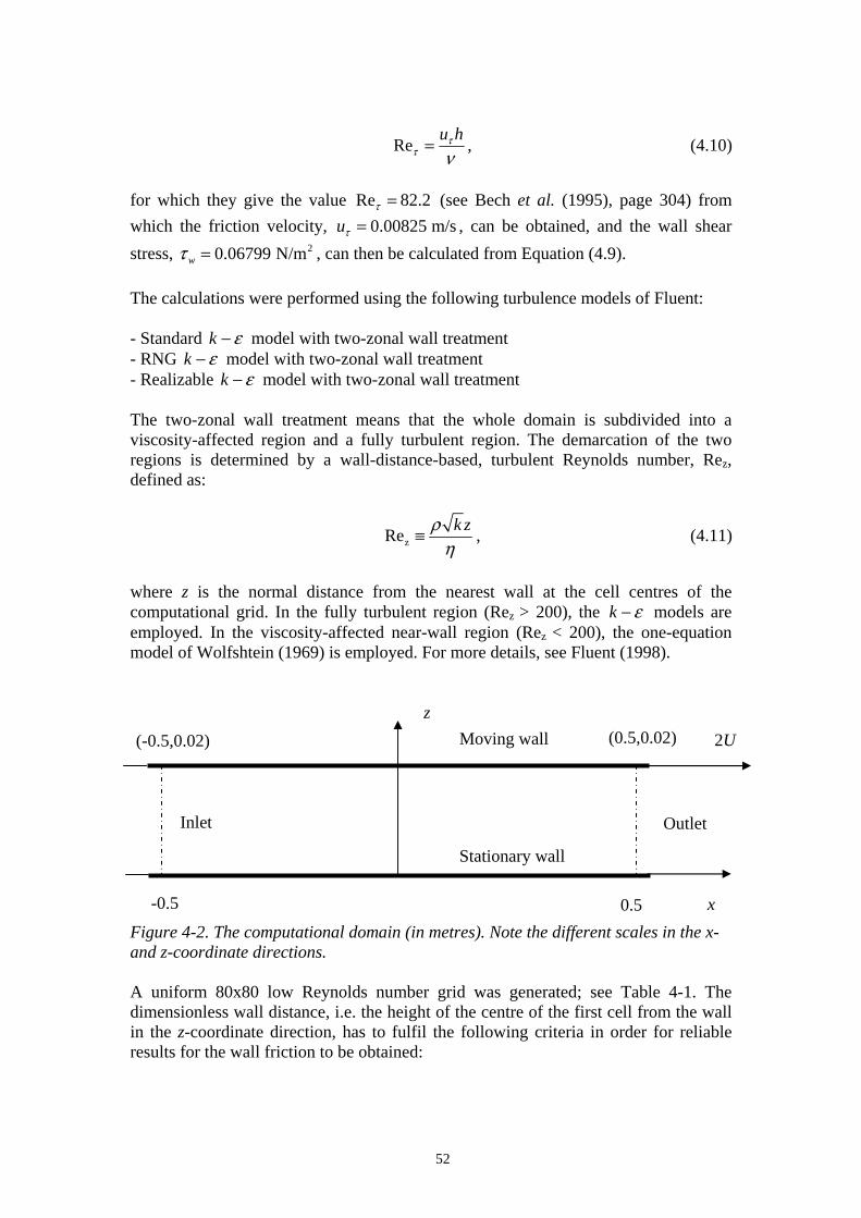
52

Re u htt n= , (4.10)

for which they give the value Re 82.2t = (see Bech et al. (1995), page 304) from which the friction velocity, 0.00825 m/sut = , can be obtained, and the wall shear stress, 20.06799 N/mwt = , can then be calculated from Equation (4.9). The calculations were performed using the following turbulence models of Fluent: - Standard k e- model with two-zonal wall treatment - RNG k e- model with two-zonal wall treatment - Realizable k e- model with two-zonal wall treatment The two-zonal wall treatment means that the whole domain is subdivided into a viscosity-affected region and a fully turbulent region. The demarcation of the two regions is determined by a wall-distance-based, turbulent Reynolds number, Rez, defined as:

zRe k zρη

≡ , (4.11)

where z is the normal distance from the nearest wall at the cell centres of the computational grid. In the fully turbulent region (Rez > 200), the k e- models are employed. In the viscosity-affected near-wall region (Rez < 200), the one-equation model of Wolfshtein (1969) is employed. For more details, see Fluent (1998). Figure 4-2. The computational domain (in metres). Note the different scales in the x- and z-coordinate directions. A uniform 80x80 low Reynolds number grid was generated; see Table 4-1. The dimensionless wall distance, i.e. the height of the centre of the first cell from the wall in the z-coordinate direction, has to fulfil the following criteria in order for reliable results for the wall friction to be obtained:

z

x

(-0.5,0.02) (0.5,0.02)

-0.5 0.5

Inlet Outlet

Stationary wall

Moving wall 2U

53

1zu

z t

n+ = £ . (4.12)

The following boundary conditions were used: velocity of the upper wall 2U = 0.261 m/s in the positive x-coordinate direction, and velocity of the lower wall is zero. For the inlet and the outlet the translationally periodic boundary condition was used. Translationally periodic boundaries are boundaries that form periodic planes in a rectilinear geometry (Fluent (1998), p. 6-93). When the flow through the periodic boundary adjacent to a fluid cell is being calculated, the flow conditions at the fluid cell adjacent to the opposite periodic plane are used (see also Section 5.3.4.3). Table 4-1. The 80x80 low Reynolds number grid ( / 50x zD D = ). Direction Number

of cells Length of the first and the last cell [m]

Length of the cell in the middle [m]

Grid expansion factor

x (-0.5 m to 0.5 m) 80 0.0125 0.0125 1 z (0 m to 0.02 m) 80 0.00025 0.00025 1

4.2.1.1 Comparison of the calculated shear stresses with the data of Bech et al. The results of the calculations were compared with the DNS data provided by Bech et al. (2000). The calculated wall shear stress using the turbulence models of Fluent are compared with the data of Bech et al. (2000) in Table 4-2. As can be seen in Table 4-2, both the standard k e- model of Fluent and the RNG k e- model of Fluent with two-zonal wall treatment give reasonable results for the wall shear stress, the error being less than 10%. In the following section the results obtained by the standard k e- model of Fluent with two-zonal wall treatment will be compared with the DNS data of Bech et al. (2000) in more detail. Table 4-2. Comparison of the calculated wall shear stress with the data of Bech et al., (2000). Bech et

al. Fluent, Standard k e- turbulence model

Fluent, RNG k e- turbulence model

Fluent, Realisable k e- turbulence model

2 [N/m ]wt 0.06799 0.063189 0.06334 0.059466

Error [%] - -7.06 -6.84 -12.54 4.2.1.2 Results of the standard k e- model of Fluent Velocity distribution The dimensionless mean velocity distribution in the streamwise direction (u-velocity) in the lower half of the channel is depicted in Figure 4-3. It can be noted that in the viscous sub-layer and buffer regions the standard k e- model of Fluent gives slightly

54

lower values for the u velocity and slightly higher values in the logarithmic region, compared with the DNS data of Bech et al. (2000).

0

0.2

0.4

0.6

0.8

1

1.2

0 0.2 0.4 0.6 0.8 1 1.2

z /h

u/U

u/U (DNS data of Bechet al. (2000))u/U (Fluent, standard k-ε turbulence model)

Figure 4-3. Dimensionless mean velocity distribution of the velocity in the x-coordinate direction in the lower half of the channel.

02468

1012141618

0.1 1 10 100

z +

u+

u+ (Bech et al.) u+ (Fluent, k-ε) u+ = z+ u+ = 2.55ln(z+)+4.5

Figure 4-4. Dimensionless mean velocity, u+, in the x-coordinate direction in the lower half of the channel as a function of the dimensionless wall distance, z+, drawn on a semi-logarithmic scale.

55

This indicates that the standard k e- model of Fluent gives slightly lower values for the shear stress at the wall than the DNS calculations of Bech et al. (2000). This is indeed the case: Bech et al. (1995) give 20.06799 N/mwt = , while Fluent gives

20.063189 N/mwt = , which is 7.06% less. The mean velocity in Figure 4-4 is plotted in a semi-logarithmic form, normalised with viscous scales as follows: / and z / .u u u zut t n+ += = In addition to the DNS data of Bech et al. (2000) and the k e- data of Fluent, the familiar logarithmic relation: lnu A z B+ += + (4.13) with the constants A and B adapted to the DNS data of Bech et al. (2000) is shown in Figure 4-4. A value of 2.55 for the constant A and a value of 4.5 for the constant B correlate well with the DNS data according to Bech et al. (1995). Turbulent magnitudes Dimensionless fluctuating velocities, ' ' '/ , / and /rms rms rmsu u v u w uτ τ τ , according to the DNS data of Bech et al. (2000), are depicted in Figure 4-5. In Figure 4-5 it can be seen that the fluctuating velocity has its highest value in the x-coordinate direction. In the other directions the fluctuating velocity has a much lower value. This indicates that the turbulent fluctuations are anisotropic. According to the DNS data of Bech et al. (2000), the average value of u'w' was negative; this is depicted schematically in Figure 4-6. This is logical for the type of flow depicted in Figure 4-1, which has

/ 0u z∂ ∂ > .

0.00

0.50

1.00

1.50

2.00

2.50

3.00

0.00 0.20 0.40 0.60 0.80 1.00

z/h

u i, r

ms/u

T u_rms/uτv_rms/uτw_rms/uτ

Figure 4-5. Distribution of the root-mean-square values of the dimensionless fluctuating velocities ' ' '/ , / and /rms rms rmsu u v u w uτ τ τ according to the DNS data of Bech et al. (2000).

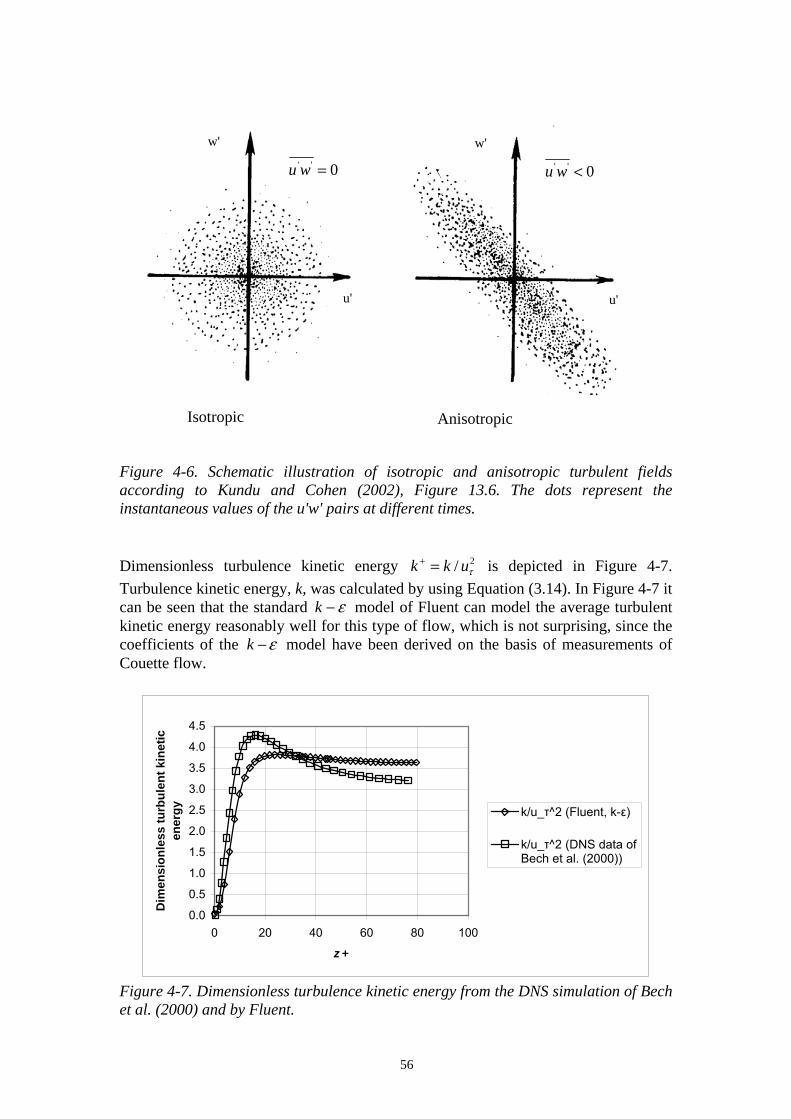
56

Figure 4-6. Schematic illustration of isotropic and anisotropic turbulent fields according to Kundu and Cohen (2002), Figure 13.6. The dots represent the instantaneous values of the u'w' pairs at different times. Dimensionless turbulence kinetic energy 2/k k ut

+ = is depicted in Figure 4-7. Turbulence kinetic energy, k, was calculated by using Equation (3.14). In Figure 4-7 it can be seen that the standard k e- model of Fluent can model the average turbulent kinetic energy reasonably well for this type of flow, which is not surprising, since the coefficients of the k ε− model have been derived on the basis of measurements of Couette flow.

0.0

0.5

1.0

1.5

2.0

2.5

3.0

3.5

4.0

4.5

0 20 40 60 80 100

z +

Dim

ensi

onle

ss tu

rbul

ent k

inet

ic

ener

gy k/u_τ^2 (Fluent, k-ε)

k/u_τ^2 (DNS data ofBech et al. (2000))

Figure 4-7. Dimensionless turbulence kinetic energy from the DNS simulation of Bech et al. (2000) and by Fluent.

w' w'

' ' 0u w <

u' u'

' ' 0u w =

Isotropic Anisotropic

57

Dimensionless turbulent and viscous stresses across the channel are depicted in Figure 4-8. Turbulent stresses are obtained from the Boussinesq approximation (3.13). With i = 1 and j = 2, and setting / 0w x∂ ∂ = :

' 't

uu wz

r h ∂- =∂

. (4.14)

It can be concluded that the calculated results of the standard k e- model of Fluent with two-zonal wall treatment correlate reasonably well with the data of Bech et al. (2000).

0.0

0.2

0.4

0.6

0.8

1.0

1.2

0.00 0.20 0.40 0.60 0.80 1.00

z /h

Dim

ensi

onle

ss R

eyno

lds

and

visc

ous

stre

sses

-ρ*u'w'rms/τ_w (Bech et al.) η*du/dz/τ_w (Bech et al.) -ρ*u'w'rms/τ_w (Fluent, k-ε) η*du/dz/τ_w (Fluent, k-ε)

Figure 4-8. Dimensionless Reynolds and viscous stresses across the channel obtained from the DNS simulation of Bech et al. (2000) and by Fluent. 4.2.2 Comparison of the results obtained by Fluent with the experimental data

of the turbulent Couette-type flow of Nakabayashi Experimental work has been performed by Nakabayashi et al. (1991) to investigate turbulent Couette-type flow with repeated longitudinal pressure gradients that are realised in a channel consisting of a wavy fixed wall on one side and a moving plane wall on the other side. This type of flow simulates the flow in high-speed journal bearings operating in turbulent conditions. The flow is two-dimensional with a constant temperature. In this section the experimental data of Nakabayashi (1993) are compared with the calculated results obtained by Fluent using the standard k ε− model with two-zonal wall treatment.

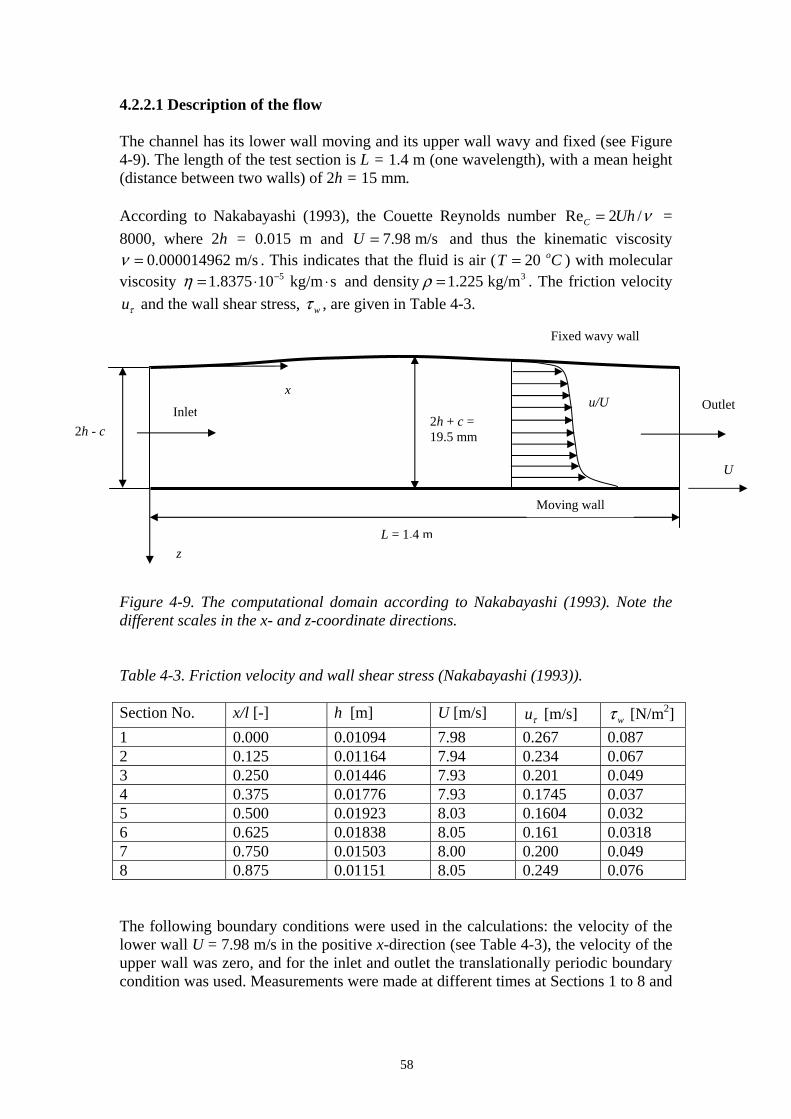
58

4.2.2.1 Description of the flow The channel has its lower wall moving and its upper wall wavy and fixed (see Figure 4-9). The length of the test section is L = 1.4 m (one wavelength), with a mean height (distance between two walls) of 2h = 15 mm. According to Nakabayashi (1993), the Couette Reynolds number Re 2 /C Uh n= = 8000, where 2h = 0.015 m and 7.98 m/sU = and thus the kinematic viscosity

0.000014962 m/sn = . This indicates that the fluid is air ( 20 oT C= ) with molecular viscosity 51.8375 10 kg/m sh -= ◊ ◊ and density 31.225 kg/mr = . The friction velocity ut and the wall shear stress, wt , are given in Table 4-3. Figure 4-9. The computational domain according to Nakabayashi (1993). Note the different scales in the x- and z-coordinate directions. Table 4-3. Friction velocity and wall shear stress (Nakabayashi (1993)). Section No. x/l [-] h [m] U [m/s] ut [m/s] wt [N/m2] 1 0.000 0.01094 7.98 0.267 0.087 2 0.125 0.01164 7.94 0.234 0.067 3 0.250 0.01446 7.93 0.201 0.049 4 0.375 0.01776 7.93 0.1745 0.037 5 0.500 0.01923 8.03 0.1604 0.032 6 0.625 0.01838 8.05 0.161 0.0318 7 0.750 0.01503 8.00 0.200 0.049 8 0.875 0.01151 8.05 0.249 0.076 The following boundary conditions were used in the calculations: the velocity of the lower wall U = 7.98 m/s in the positive x-direction (see Table 4-3), the velocity of the upper wall was zero, and for the inlet and outlet the translationally periodic boundary condition was used. Measurements were made at different times at Sections 1 to 8 and

z

x

Inlet Outlet

L = 1.4 m

2h + c = 19.5 mm 2h - c

U

u/U

Fixed wavy wall

Moving wall

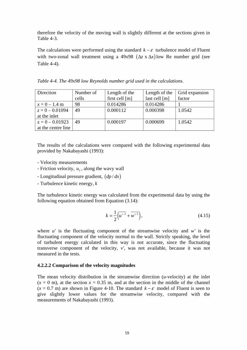
59

therefore the velocity of the moving wall is slightly different at the sections given in Table 4-3. The calculations were performed using the standard k e- turbulence model of Fluent with two-zonal wall treatment using a 49x98 ( )x z xD D low Re number grid (see Table 4-4). Table 4-4. The 49x98 low Reynolds number grid used in the calculations. Direction Number of

cells Length of the first cell [m]

Length of the last cell [m]


x = 0 – 1.4 m 98 0.014286 0.014286 1 z = 0 – 0.01094 at the inlet

49 0.000112 0.000398 1.0542

z = 0 – 0.01923 at the centre line

49 0.000197 0.000699 1.0542

The results of the calculations were compared with the following experimental data provided by Nakabayashi (1993): - Velocity measurements - Friction velocity, ut , along the wavy wall - Longitudinal pressure gradient, ( )/dp dx - Turbulence kinetic energy, k The turbulence kinetic energy was calculated from the experimental data by using the following equation obtained from Equation (3.14):

( )2 21 ' '2

k u w= + , (4.15)

where u' is the fluctuating component of the streamwise velocity and w' is the fluctuating component of the velocity normal to the wall. Strictly speaking, the level of turbulent energy calculated in this way is not accurate, since the fluctuating transverse component of the velocity, v', was not available, because it was not measured in the tests. 4.2.2.2 Comparison of the velocity magnitudes The mean velocity distribution in the streamwise direction (u-velocity) at the inlet (x = 0 m), at the section x = 0.35 m, and at the section in the middle of the channel (x = 0.7 m) are shown in Figure 4-10. The standard k e- model of Fluent is seen to give slightly lower values for the streamwise velocity, compared with the measurements of Nakabayashi (1993).

60

0

0.005

0.01

0.015

0.02

0.025

0 1 2 3 4 5 6 7 8 9

u [m/s]z

[m]

u, Nakabayashi, x = 0 m u, Fluent, k-ε, x = 0 mu, Nakabayashi, x = 0.35 m u, Fluent, k-ε, x = 0.35 mu, Nakabayashi, x = 0.7 m u, Fluent, k-ε, x = 0.7 m

Figure 4-10. Comparison of the calculated streamwise velocity at x = 0 m (inlet), at x = 0.35 m and at x = 0.7 m (CL) with the data of Nakabayashi (1993). 4.2.2.3 Comparison of turbulence kinetic energy The turbulence kinetic energy, k, at x = 0 m (inlet), and at x = 0.7 m in the middle of the channel is depicted in Figures 4-11 and 4-12. The calculated results are not quite comparable to the measured ones as the fluctuating transverse component of velocity, v', was not measured in the tests.

0

0.05

0.1

0.15

0.2

0.25

0.3

0.35

0 0.002 0.004 0.006 0.008 0.01 0.012

z [m]

k [m

2/s2

]

k (Nakabayashi)k (Fluent, k-ε)

Figure 4-11. Comparison of the turbulence kinetic energy k at x = 0 m (inlet) obtained by Fluent with the experimental data of Nakabayashi (1993).

61

0

0.05

0.1

0.15

0.2

0.25

0.3

0.35

0 0.005 0.01 0.015 0.02 0.025

y [m]

k [m

2/s2

]

k(Nakabayashi)k(Fluent, k-ε)

Figure 4-12. Comparison of the turbulent kinetic energy k at x = 0.7 m (in the middle of the channel) obtained by Fluent with the experimental data of Nakabayashi (1993). 4.2.2.4 Comparison of the friction velocities The friction velocity /wut t r= at the upper wavy wall obtained by Fluent is depicted in Figure 4-13 and shows qualitatively good correlation with the experimental data of Nakabayashi (1993).

0

0.05

0.1

0.15

0.2

0.25

0.3

0.35

0 0.5 1 1.5

x [m]

Fric

tion

velo

city

[m/s

]

u_τ (Nakabayashi)u_τ (Fluent, k-ε)

Figure 4-13. Comparison of the friction velocity at the upper wall obtained by Fluent with the experimental data of Nakabayashi (1993).

62

4.2.2.5 Comparison of the pressure gradients The pressure gradient in the x-coordinate direction, /dp dx , obtained by Fluent is shown in Figure 4-14 and shows qualitatively good correlation with the experimental data of Nakabayashi (1993).

-5.00E+01

-4.00E+01

-3.00E+01

-2.00E+01

-1.00E+01

0.00E+00

1.00E+01

2.00E+01

3.00E+01

4.00E+01

0 0.5 1 1.5

x [m]

dp/d

x dp/dx (Nakabayashi)dp/dx (Fluent, k-ε)

Figure 4-14. Comparison of the longitudinal pressure gradient obtained by Fluent with the experimental data of Nakabayashi (1993). 4.3 Summary of Chapter 4 The turbulence models of Fluent were validated against the direct numerical simulation data of Bech et al. (1995 and 2000) for plane-turbulent Couette flow. The standard k ε− turbulence model of Fluent with two-zonal wall treatment was found to give a reasonably good estimate for the wall shear stress for the simulation case of Bech et al. (1995). The velocity distribution in the channel calculated using Fluent correlates very well with the DNS data of Bech et al. (2000). The calculations of Bech et al. (2000) showed turbulent fluctuations to be anisotropic and the fluctuating velocity has its highest value in the x-coordinate direction. The results of the calculations obtained by Fluent showed that the standard k e- model of Fluent can model the average turbulent kinetic energy reasonably well for this type of flow. The calculation results of Fluent were also compared with the experimental data of Nakabayashi (1993) for Couette flow with pressure gradient. The standard k e- model of Fluent gave slightly lower values for the streamwise velocity compared with the experimental data of Nakabayashi (1993). The results of the turbulent kinetic energy calculations obtained using Fluent did not correlate so well with the data of Nakabayashi (1993). However, the friction velocity and the pressure gradient obtained by Fluent showed a reasonably good correlation with the data of Nakabayashi (1993). The final conclusion of this chapter is that Fluent can be used for the calculation of this type of flow.

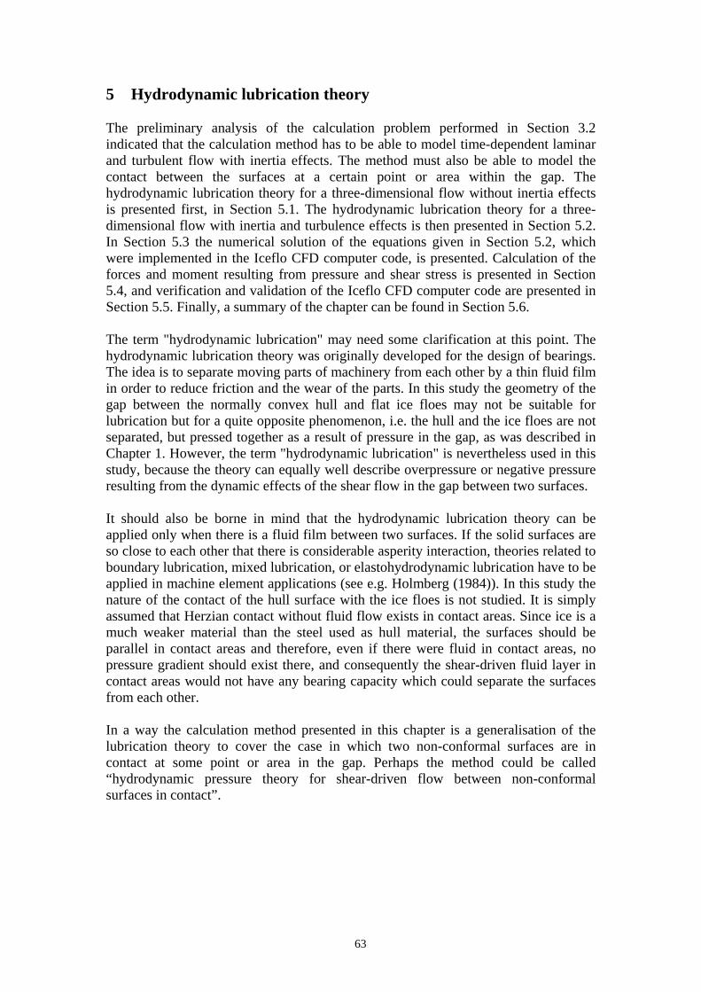
63

5 Hydrodynamic lubrication theory The preliminary analysis of the calculation problem performed in Section 3.2 indicated that the calculation method has to be able to model time-dependent laminar and turbulent flow with inertia effects. The method must also be able to model the contact between the surfaces at a certain point or area within the gap. The hydrodynamic lubrication theory for a three-dimensional flow without inertia effects is presented first, in Section 5.1. The hydrodynamic lubrication theory for a three-dimensional flow with inertia and turbulence effects is then presented in Section 5.2. In Section 5.3 the numerical solution of the equations given in Section 5.2, which were implemented in the Iceflo CFD computer code, is presented. Calculation of the forces and moment resulting from pressure and shear stress is presented in Section 5.4, and verification and validation of the Iceflo CFD computer code are presented in Section 5.5. Finally, a summary of the chapter can be found in Section 5.6. The term "hydrodynamic lubrication" may need some clarification at this point. The hydrodynamic lubrication theory was originally developed for the design of bearings. The idea is to separate moving parts of machinery from each other by a thin fluid film in order to reduce friction and the wear of the parts. In this study the geometry of the gap between the normally convex hull and flat ice floes may not be suitable for lubrication but for a quite opposite phenomenon, i.e. the hull and the ice floes are not separated, but pressed together as a result of pressure in the gap, as was described in Chapter 1. However, the term "hydrodynamic lubrication" is nevertheless used in this study, because the theory can equally well describe overpressure or negative pressure resulting from the dynamic effects of the shear flow in the gap between two surfaces. It should also be borne in mind that the hydrodynamic lubrication theory can be applied only when there is a fluid film between two surfaces. If the solid surfaces are so close to each other that there is considerable asperity interaction, theories related to boundary lubrication, mixed lubrication, or elastohydrodynamic lubrication have to be applied in machine element applications (see e.g. Holmberg (1984)). In this study the nature of the contact of the hull surface with the ice floes is not studied. It is simply assumed that Herzian contact without fluid flow exists in contact areas. Since ice is a much weaker material than the steel used as hull material, the surfaces should be parallel in contact areas and therefore, even if there were fluid in contact areas, no pressure gradient should exist there, and consequently the shear-driven fluid layer in contact areas would not have any bearing capacity which could separate the surfaces from each other. In a way the calculation method presented in this chapter is a generalisation of the lubrication theory to cover the case in which two non-conformal surfaces are in contact at some point or area in the gap. Perhaps the method could be called “hydrodynamic pressure theory for shear-driven flow between non-conformal surfaces in contact”.

64

5.1 Hydrodynamic lubrication theory for a three-dimensional flow without inertia effects

Changing back to non-dimensional variables by inserting Equations (3.16), (3.17), and (3.19) into Equations (3.25) and (3.26) and assuming negligible inertia effects by requiring that *Re 0→ , Equations (3.25) and (3.26) can be further simplified to read:

2

2

2

2

d

d

p ux zp vy z

h

h

∂ ∂=∂ ∂∂ ∂=∂ ∂

(5.1)

0u v wx y z

∂ ∂ ∂+ + =∂ ∂ ∂

. (5.2)

The equations of momentum (5.1) can now be integrated twice with respect to z, and the integration constants can be calculated using the boundary conditions, assuming that the molecular forces between the solid wall and the neighbouring molecules in the fluid are sufficiently strong to prevent them from being detached by the shear stresses developed in the fluid film; see e.g. Holmberg (1984):

0, 0 at 0

, 0 at .u v zu U v z h

= = == = =

(5.3)

When the resulting expressions for the velocity components are inserted into the equation of continuity (5.2), and when this is then integrated across the film (see e.g. Szeri (1998), pp. 73-76), the Reynolds equation for three-dimensional flow in a gap is obtained:

3 3

6 12d dp ph h h hUx x y y x tη η⎛ ⎞ ⎛ ⎞∂ ∂∂ ∂ ∂ ∂+ = +⎜ ⎟ ⎜ ⎟∂ ∂ ∂ ∂ ∂ ∂⎝ ⎠ ⎝ ⎠

. (5.4)

Equation (5.4) can be written in a more general form, which takes turbulent flow into account (see e.g. Szeri (1998), p. 254):

3 3

2d d

x y

p ph h U h hx k x y k y x tη η

⎛ ⎞⎛ ⎞∂ ∂∂ ∂ ∂ ∂+ = +⎜ ⎟⎜ ⎟ ⎜ ⎟∂ ∂ ∂ ∂ ∂ ∂⎝ ⎠ ⎝ ⎠, (5.5)

where xk is the effect of turbulent viscosity in the x-coordinate direction and yk is the effect of turbulent viscosity in the y-coordinate direction (see Section 5.2.4). If the flow is laminar, 12x yk k= = . Equation (5.5) is valid if the following assumptions are valid: the pressure is constant through the thickness of the film; the radii of curvature of surfaces are large compared with the film thickness; there is no slip at the boundaries; the fluid is Newtonian; fluid inertia is neglected, and the viscosity is constant throughout the film thickness (see Cameron (1976), p. 21).

65

Equation (5.5) is a non-homogeneous partial differential equation of two variables, h and dp . If the height of the gap is assumed to be known, a numerical solution to Equation (5.5) can be obtained in the same way as described in Pinkus and Sternlicht (1961), p. 80. Using a rectangular grid, the first three terms of Equation (5.5) were discretised using the finite difference method and the last term was discretised using Euler’s method. The pressure field can then be solved from the obtained Poisson-type equation. The mean velocity of the fluid flow in the gap can be obtained from the following equations:

2

2d

mx

ph Uuk xη

∂= − +∂

(5.6)

2

dm

y

phvk yη

∂= −∂

(5.7)

5.2 Hydrodynamic lubrication theory for a three-dimensional flow with

inertia effects The Reynolds averaged Navier-Stokes equations (3.11) and (3.12) can be written in the x-, y-, and z-directions as follows:

( ) ( ) ( )

( ) ( ) ( )2 2 2' ' ' ' ' '

2 2 2d

u u u v u w ut x y z

p u u u u u v u wux x y z x y z

r r r r

h r r r

∂ ∂ ∂ ∂+ + + =∂ ∂ ∂ ∂

Ê ˆ∂ ∂ ∂ ∂ ∂ ∂ ∂- + + + - - -Á ˜∂ ∂ ∂ ∂ ∂ ∂ ∂Ë ¯

(5.8)

( ) ( ) ( )

( ) ( ) ( )2 2 2' ' ' ' ' '

2 2 2d

v u v v v w vt x y z

p v v v u v v v w vy x y z x y z

r r r r

h r r r

∂ ∂ ∂ ∂+ + + =∂ ∂ ∂ ∂

Ê ˆ∂ ∂ ∂ ∂ ∂ ∂ ∂- + + + - - -Á ˜∂ ∂ ∂ ∂ ∂ ∂ ∂Ë ¯

(5.9)

( ) ( ) ( )

( ) ( ) ( )2 2 2' ' ' ' ' '

2 2 2d

w u w v w w wt x y z

p w w w u w v w w wz x y z x y z

r r r r

h r r r

∂ ∂ ∂ ∂+ + + =∂ ∂ ∂ ∂

Ê ˆ∂ ∂ ∂ ∂ ∂ ∂ ∂- + + + - - -Á ˜∂ ∂ ∂ ∂ ∂ ∂ ∂Ë ¯

(5.10)

0u v wx y z

∂ ∂ ∂+ + =∂ ∂ ∂

. (5.11)

Equations (5.8) to (5.10) can be simplified by making the following boundary layer approximations for certain terms (see Kundu and Cohen (2002), p. 315):

2 2

2 2 and x z x z

∂ ∂ ∂ ∂∂ ∂ ∂ ∂

(5.12)

66

and

2 2

2 2 and y z y z

∂ ∂ ∂ ∂∂ ∂ ∂ ∂

, (5.13)

which means that the variation of a quantity is much larger across the boundary layer than along it. Assuming that the length scale (h/l) = O(10-6), Equation (5.10) can be completely dispensed with; see Chapter 3. Taking these assumptions into account, the reduced Navier-Stokes equations (5.8) to (5.11) can be written in the following form, also known as Prandtl's turbulent boundary-layer equations:

( ) ( ) ( ) ( )2' '

2dpu uu u v u w u wu

t x y z x z zr r r r h r∂∂ ∂ ∂ ∂ ∂ ∂+ + + = - + -∂ ∂ ∂ ∂ ∂ ∂ ∂

(5.14)

( ) ( ) ( ) ( )2' '

2dpv vu v v v w v w v

t x y z y z zr r r r h r∂∂ ∂ ∂ ∂ ∂ ∂+ + + = - + -∂ ∂ ∂ ∂ ∂ ∂ ∂

(5.15)

0 dpz

∂≈ −∂

(5.16)

0u v wx y z

∂ ∂ ∂+ + =∂ ∂ ∂

. (5.17)

As Equation (5.16) shows, the pressure is constant across the fluid film, as was concluded in Chapter 3. Thus: ( ), ,d dp p x y t= . (5.18) Equations (5.14), (5.15), and (5.17) can be further simplified by integrating them across the gap height, h. In this way the dimensions of the calculation problem can be reduced from three to two, which greatly simplifies the numerical calculation procedure. 5.2.1 Integration of the continuity equation The continuity equation (5.17) is first integrated across the gap, which gives (see Salonen (1987), pp. 6.11.3 to 6.11.5):

2 10 0

0h hu vdz dz w w

x y∂ ∂+ + - =∂ ∂Ú Ú , (5.19)

where the subscripts 1 and 2 refer to the lower and upper surfaces respectively. According to the Leibnitz rule, Equation (5.19) can be written as follows:

( ) ( ) 2 2 2 1 0m mh hhu hv u v w w

x y x y∂ ∂ ∂ ∂+ − − + − =∂ ∂ ∂ ∂

, (5.20)

67

where the mean velocity of the flow in the x-coordinate direction has been defined as follows:

0

1 h

mu udzh

= ∫ (5.21)

and the mean velocity of the flow in the y-coordinate direction as follows:

0

1 h

mv vdzh

= ∫ . (5.22)

From the kinematics of the surfaces and taking the no-slip conditions at the walls into account, the continuity equation integrated across the fluid film can be written:

( ) ( ) 0m mhhu hv

x y t∂ ∂ ∂+ + =∂ ∂ ∂

(5.23)

5.2.2 Integration of the momentum equations Next, the momentum equations in the directions of the x- and y-coordinate axes are considered. Integrating Equations (5.14) and (5.15) gives, taking into account Equation (5.18):

( ) ( ) 2 2 1 1

0 0 0

' ' ' '2 2 1 1

2 1

h h h

d

u dz u u dz v u dz w u w ut x y

p u uh w u w ux z z

r r r r r

h h r r

∂ ∂ ∂+ + + - =∂ ∂ ∂

∂ ∂ ∂Ê ˆ Ê ˆ- + - - +Á ˜ Á ˜Ë ¯ Ë ¯∂ ∂ ∂

Ú Ú Ú (5.24)

and

( ) ( ) 2 2 1 1

0 0 0

' ' ' '2 2 1 1

2 1

,

h h h

d

v dz u v dz v v dz w v w vt x y

p v vh w v w vy z z

r r r r r

h h r r

∂ ∂ ∂+ + + - =∂ ∂ ∂

∂ ∂ ∂Ê ˆ Ê ˆ- + - - +Á ˜ Á ˜Ë ¯ Ë ¯∂ ∂ ∂

Ú Ú Ú (5.25)

Using the Leibnitz rule, assuming no-slip conditions at the walls, and taking into account the fact that the turbulent fluctuations vanish at z = 0 and z = h, Equations (5.24) and (5.25) can be written as follows:

( )2 1

xyxx dm

II p u uhu ht x y x z z

r r r h h∂∂ ∂∂ ∂ ∂Ê ˆ Ê ˆ+ + = - + -Á ˜ Á ˜Ë ¯ Ë ¯∂ ∂ ∂ ∂ ∂ ∂

(5.26)

and

( )2 1

,yy yx dm

I I p v vhv ht y x y z z

r r r h h∂ ∂ ∂∂ ∂ ∂Ê ˆ Ê ˆ+ + = - + -Á ˜ Á ˜Ë ¯ Ë ¯∂ ∂ ∂ ∂ ∂ ∂

(5.27)

where

68

0 0 0

, and h h h

xx xy yx yyI uudz I I uvdz I vvdz= = = =∫ ∫ ∫ . (5.28)

To proceed further, assumptions must be made about the distribution of velocity within the fluid film in the gap. Constantinescu (1970) and Constantinescu and Galetuse (1974) assume that the shape of the mean velocity distribution in the film is unaffected by inertia. Now the method given in Leschziner (1976) is followed to determine the velocity profiles, ( ) ( ) andu z v z . Neglecting the inertia terms, Equations (5.26) and (5.27) can be written approximately as follows:

dpuz z x

η ∂∂ ∂⎛ ⎞ =⎜ ⎟∂ ∂ ∂⎝ ⎠ (5.29)

and

dpvz z y

η ∂∂ ∂⎛ ⎞ =⎜ ⎟∂ ∂ ∂⎝ ⎠, (5.30)

where the velocity and pressure do not now, of course, include inertia effects. Integrating Equations (5.29) and (5.30) twice with respect to z allows us to write the following equations for the velocity distributions in the x- and y-coordinate directions:

( )2

1 22dpzu z C z C

xη∂= + +∂

(5.31)

and

( )2

3 4 ,2

dpzv z C z Cyη

∂= + +∂

(5.32)

where 1 2 3 4, , and C C C C are integration constants, which can be determined by using the no-slip conditions on the walls; see the equations in (5.3). After some manipulation it can be written:

( ) ( )2

dpz zu z z h Ux hη

∂= − +∂

(5.33)

and

( ) ( )2

dpzv z z hyη

∂= −∂

. (5.34)

The pressure gradient can now be eliminated by first inserting (5.33) into (5.21) and (5.34) into (5.22), which means it can be written:

2

122

dm

p U ux h

η∂ ⎛ ⎞= −⎜ ⎟∂ ⎝ ⎠ (5.35)

and

2

12dm

p vy h

η∂ = −∂

, (5.36)

and inserting (5.35) into (5.33), and (5.36) into (5.34), it can finally be written:

69

( ) ( )2

2 3 6 mz z zu z U u Uh h h

⎛ ⎞= − − +⎜ ⎟⎝ ⎠

(5.37)

and

( ) 6 1mv z zv zh h

⎛ ⎞= −⎜ ⎟⎝ ⎠

. (5.38)

Now , and xx xy yx yyI I I I= can be calculated by inserting (5.37) and (5.38) into the equations in (5.28):

2 26 1 25 5 15xx m mI h u Uu U⎛ ⎞= − +⎜ ⎟

⎝ ⎠, (5.39)

6 15 10xy yx m m mI I u v Uv⎛ ⎞= = −⎜ ⎟

⎝ ⎠, (5.40)

265yy mI hv= . (5.41)

5.2.3 The equations of Constantinescu Recalling the integral form of the continuity equation (5.23) and inserting Equations (5.37) to (5.41) into Equations (5.26) and (5.27), the Navier-Stokes equations integrated across the fluid film can be obtained:

( ) ( ) ( )2 2mm m m m m

u hu h U h u Uh u v h Uv h

t x yρ ρ α β γ ρ α δ

∂ ∂ ∂+ + − + − +∂ ∂ ∂

02

d xm

p k Uh ux h

η∂ ⎛ ⎞+ + − =⎜ ⎟∂ ⎝ ⎠ (5.42)

( ) ( ) ( )2 0ym dm m m m m

kv h pu v h Uu h v h h vt x y y h

ηρ ρ α δ ρ α

∂ ∂∂ ∂+ − + + + =∂ ∂ ∂ ∂

(5.43)

( ) ( ) 0m mu h v h hx y t

∂ ∂ ∂+ + =∂ ∂ ∂

, (5.44)

where 1.2, =0.133, =0.2, =0.1 and 12x yk kα β γ δ= = = , (5.45) which can be used to calculate laminar three-dimensional flow with inertia effects in a gap between two surfaces. These equations were originally given by Constantinescu and Galetuse (1974) for steady flow. Leschziner (1976) also presented the derivation of the equations for steady laminar flow. According to Constantinescu and Galetuse (1982), the equations can be used for the calculation of turbulent flow by setting:

70

( ) ( )0.367 0.431, 0.885 2 Re , , 0 and 1.95 2 Re ,C Cx y x yα β γ δ− −

= ≅ ⋅ = ≅ ⋅⎡ ⎤ ⎡ ⎤⎣ ⎦ ⎣ ⎦ . (5.46) The turbulence models kx and ky are given in Section 5.2.4 below. The advantage of solving Equations (5.42) to (5.44) instead of solving the "full" Navier-Stokes equations (3.7) and (3.8) is clear: the solution of the three-dimensional fluid flow has been reduced to the solution of a two-dimensional fluid flow problem. In the same manner the solution of a two-dimensional fluid flow has been reduced to the solution of a one-dimensional fluid flow problem. This reduces the required computing time considerably. The grid generation is also much easier when there is no need to generate the grid in the vertical direction. It should be clarified that in the following a three-dimensional fluid flow problem will be continued to be called "three-dimensional" even if it is solved using the two- dimensional equations (5.42) to (5.44), since the real flow is three-dimensional. The same applies to a two-dimensional fluid flow problem. 5.2.4 The turbulence models Three turbulence models were considered in this study. The model of Constantinescu (see Constantinescu and Galetuse (1974)) is based on the mixing length approach:

( )( )

0.9

0.96

12 0.0136 2 Re

12 0.0043 2 Rex C

y C

k

k

= + ⋅

= + ⋅ (5.47)

The turbulence model of Hirs (1973) is based on bulk flow theory:

( )( )

0.75

0.75

0.0687 2 Re

0.0392 2 Rex C

y C

k

k

= ⋅

= ⋅ (5.48)

The turbulence model of Ng and Pan (1965) is based on the eddy viscosity profile of Reichardt (see e.g. Szeri (1998), p. 247). Taylor (1970) presents the Ng and Pan model in the following manner:

( )( )

12 2 Re

12 2 Re ,

x

y

x x C

y y C

k K

k K

η

η

= + ⋅

= + ⋅ (5.49)

where , , and x y x yK K η η are given in Table 5-1. Table 5-1. Coefficients of the Ng and Pan turbulence model. xK xη yK yη ReC>50000 0.0388 0.80 0.0213 0.80 10000<ReC<50000 0.0250 0.84 0.0136 0.84 5000<ReC<10000 0.0250 0.84 0.0088 0.88 ReC<5000 0.0039 1.06 0.0021 1.06

71

0.001

0.01

0.1

11 10 100 1000 10000 100000

ReC

1/k x

Constantinescu (x-dir.) Hirs (x-dir) Ng & Pan (x-dir.)

Figure 5-1. Comparison of the turbulent viscosity coefficient kx of the turbulence models of Constantinescu, Hirs, and Ng and Pan.

0.001

0.01

0.1

11 10 100 1000 10000 100000

ReC

1/k y

Constantinescu (y-dir.) Hirs (y-dir.) Ng & Pan (y-dir.)

Figure 5-2. Comparison of the turbulent viscosity coefficient ky of the turbulence models of Constantinescu, Hirs, and Ng and Pan. The turbulent viscosity coefficients kx and ky of the three turbulence models are compared in Figures 5-1 and 5-2. In these figures it can be seen that the models of Constantinescu and Ng and Pan approach the laminar flow value 12x yk k= = when ReC approaches zero. In the model of Hirs, xk approaches 12 at about ReC = 500 and

72

yk approaches 12 at about ReC = 1000. The turbulence models of Constantinescu and Hirs were implemented in the Iceflo CFD code, since the model of Ng and Pan gives almost identical results up to a Couette Reynolds number of 20,000 as the model of Constantinescu. 5.2.5 Flow film cavitation If the fluid is contaminated it will cavitate when the absolute pressure drops below the saturation pressure of the dissolved gases (gaseous cavitation). Vapour cavitation (boiling) occurs when the absolute pressure falls to the vapour pressure (Szeri (1998), p. 98). In such cases the flow film cannot be in direct contact with the surrounding surfaces. Flow film vapour cavitation exists if the absolute pressure, i.e. the sum of the atmospheric pressure, the hydrostatic pressure, and the dynamic pressure is less than the vapour pressure of the fluid: atm h d vp p p p+ + < , (5.50) where patm is the atmospheric pressure, ph is the hydrostatic pressure, and pv is the vapour pressure of the fluid. The atmospheric pressure at sea level is about 101.3 kPa (Truckenbrodt (1968)) and the vapour pressure of water is 0.61 kPa at 0oC (White (1991)). 5.2.6 Flow film separation As a result of the simplifications made when deriving Equations (5.42) to (5.44), some information on the flow is also lost, i.e. the vertical distribution of the velocity. This means that the hydrodynamic lubrication theory cannot predict flow separation, and for the same reason the calculation of the shear stresses on the walls is inaccurate for a separating flow. However, for laminar flow, the separation condition will be (see Constantinescu et al. (1975)):

0

0; 3m

z

u Uuz =

∂⎛ ⎞ = =⎜ ⎟∂⎝ ⎠. (5.51)

For turbulent flow the following quantity can be defined (Constantinescu et al. (1975)):

*

**H δδ

= , (5.52)

where *δ is the displacement thickness:

*

0

1 1h

muu dz hU U

δ ⎛ ⎞⎛ ⎞= − = −⎜ ⎟ ⎜ ⎟⎝ ⎠ ⎝ ⎠∫ (5.53)

and **δ is the momentum thickness:

73

**2

0

1h

m xxu Iu u dz h hU U U U

δ ⎛ ⎞⎛ ⎞= − = −⎜ ⎟ ⎜ ⎟⎝ ⎠ ⎝ ⎠∫ . (5.54)

Now: 2 2

xx m mI u h U h u Uhα β γ= + − , (5.55) see the second term of Equation (5.42). Inserting Equation (5.55) into Equation (5.54) with the parameters , and α β γ given in the equations in (5.46), and then inserting Equations (5.53) and (5.54) into Equation (5.52) the following expression can be obtained:

( )

12

0.367 0.367

0.88512 Re

m m m

C

u u uHU U U h

−⎡ ⎤⎛ ⎞ ⎛ ⎞= − − −⎢ ⎥⎜ ⎟ ⎜ ⎟

⎝ ⎠ ⎝ ⎠ ⋅⎢ ⎥⎣ ⎦. (5.56)

Boundary layer experiments show that separation occurs for a certain value H = Hs. According to Constantinescu et al. (1975) for air films Hs = 2.69. Inserting this value into Equation (5.56) the following magnitude of the mean velocity, um, at the point of separation can be obtained:

( )0.367

25.60.686 0.186 2.8562 Re

msC

u U⎡ ⎤⎢ ⎥= − −

⋅⎢ ⎥⎣ ⎦. (5.57)

The calculations performed in Section 5.5.2.2 indicated, however, that Equation (5.57) predicts the point of separation poorly when the fluid is water. Better results were obtained using the value of 7.45 for Hs. Inserting this value into Equation (5.56) gives the following magnitude for the mean velocity, um, at the point of separation, when the fluid is water:

( )0.367

196.470.567 0.067 41.62 Re

msC

u U⎡ ⎤⎢ ⎥= − −

⋅⎢ ⎥⎣ ⎦. (5.58)

5.3 Numerical solution of the equations of Constantinescu Three numerical procedures can be found in the literature to solve Equations (5.42) to (5.44) (Constantinescu and Galetuse (1982)). One possibility is to replace the unknown velocities, and m mu v , with a stream function ψ in order to obtain the unknowns ψ and dp (see e.g. Smalley et al. (1974)). Another idea is to retain the primitive variables , ,m m du v p as unknowns and to use a marching procedure coupled with an initial guess as to the pressure field and an iteration scheme to correct mass imbalances through new values for the pressure distribution, i.e. the control volume method (see Leschziner (1976), Launder and Leschziner (1978a and 1978b), and Arghir and Frêne (2001)). The third option would be to solve a pressure equation similar to that obtained when no inertia forces are considered, coupled to an iteration

74

scheme to account for inertial terms as source terms (see Constantinescu and Galetuse (1982)). The first option was not tried by the author, because of possible difficulties in presenting all the required boundary conditions via the use of a stream function. The third option was tried using the finite difference method, but was rejected because of convergence problems. Convergence of the iteration procedure was obtained only for flow with a very low Couette Reynolds number, ReC. Finally, the second option, retaining the primitive variables, was selected. The Iceflo computer code was written to solve Equations (5.42) to (5.44). The code can be used to calculate the velocity of the flow, the pressure, and the shear stress in the gap between the hull surface and a rectangular ice floe. Both stationary and time-dependent calculation of the flow are possible. Instead of using the control volume method, as was done by Leschiner (1976) and by Arghir and Frêne (2001), the numerical solution method presented in this study is based on the finite difference method given in Griebel et al. (1998). The solution method uses the MAC (marker-and-cell) method first proposed by Harlow and Welch (1965). The MAC scheme, like most of the numerical schemes developed for computational fluid dynamics problems, can be characterised as an operator splitting algorithm (Hu in Kundu and Cohen (2002)). The operator splitting algorithm divides each time step into several substeps. Each substep solves one part of the operator and thus decouples the numerical difficulties associated with each part of the operator. A more detailed description of the numerical solution scheme is given in the following sections. 5.3.1 Solution of the momentum equations The time-dependent terms of Equations (5.42) and (5.43) are first considered:

( )m mm

u h u hh ut t t

ρ ρ ρ∂ ∂ ∂= +

∂ ∂ ∂ (5.59)

( )m mm

v h v hh ut t t

ρ ρ ρ∂ ∂ ∂= +

∂ ∂ ∂. (5.60)

The time derivatives of um and vm on the right-hand side of Equations (5.59) and (5.60) can be discretised using Euler's method:

( )1 ( 1) ( )n n n

m m mu u ut t

+ +∂ −⎡ ⎤ ≈⎢ ⎥∂ Δ⎣ ⎦ (5.61)

( 1) ( 1) ( )n n n

m m mv v vt t

+ +∂ −⎡ ⎤ ≈⎢ ⎥∂ Δ⎣ ⎦, (5.62)

where the superscript n denotes the value of the variable at time tn and (n+1) denotes the value of the variable at the next time step, after the period of time tΔ has passed.

75

Using Equations (5.61) and (5.62), Equations (5.42) and (5.43) can now be written in the following form:

( )1n dm

ptu Fxρ

+ ∂Δ= −∂

(5.63)

( )1n dm

ptv Gyρ

+ ∂Δ= −∂

, (5.64)

where

( ) ( )( ) 2 2[nm m m m m m

tF u u h U h u Uh u v h Uv hh x y

ρ α β γ ρ α δρΔ ∂ ∂= − + − + − +

∂ ∂

2

]xm m

k U hu uh t

η ρ ∂⎛ ⎞+ − +⎜ ⎟ ∂⎝ ⎠ (5.65)

and

( ) ( )( ) 2 ][ ynm m m m m m m

kt hG v u v h Uv h v h v vh x y h t

ηρ α δ ρ α ρ

ρΔ ∂ ∂ ∂= − − + + +

∂ ∂ ∂. (5.66)

If F and G are evaluated at time tn , and /dp x∂ ∂ and /dp y∂ ∂ at time tn+1, the following time-discretised equations of momentum are obtained:

( ) ( )( )1

1n

n n dm

ptu Fxρ

++ ∂Δ= −

∂ (5.67)

( ) ( )( )1

1n

n n dm

ptv Gyρ

++ ∂Δ= −

∂. (5.68)

A staggered rectangular grid is used to discretise Equations (5.67) and (5.68) with respect to position (see Figure 5-3). The velocity components in the x-coordinate direction,

,i jmu , in the cells of the calculation domain are calculated at the right-hand

edge of the cells, the velocities in the y-coordinate direction, ,i jmv , are calculated at the

upper edges of the cells, and the pressure, ,i jdp , is calculated in the middle of the cells,

in order to avoid pressure fluctuations during the iteration process. A calculation domain surrounded by one row of ghost cells is depicted in Figure 5-4. The ghost cells are used to define the boundary conditions at the edges of the calculation domain. Compass notation is applied to assign names for the edges of the calculation domain: the lower edge in Figure 5-4 is called the southern edge, the upper edge is called the northern edge, the edge on the left is called the western edge, and the edge on the right is called the eastern edge of the calculation domain. The fluid is assumed to flow from west to east.

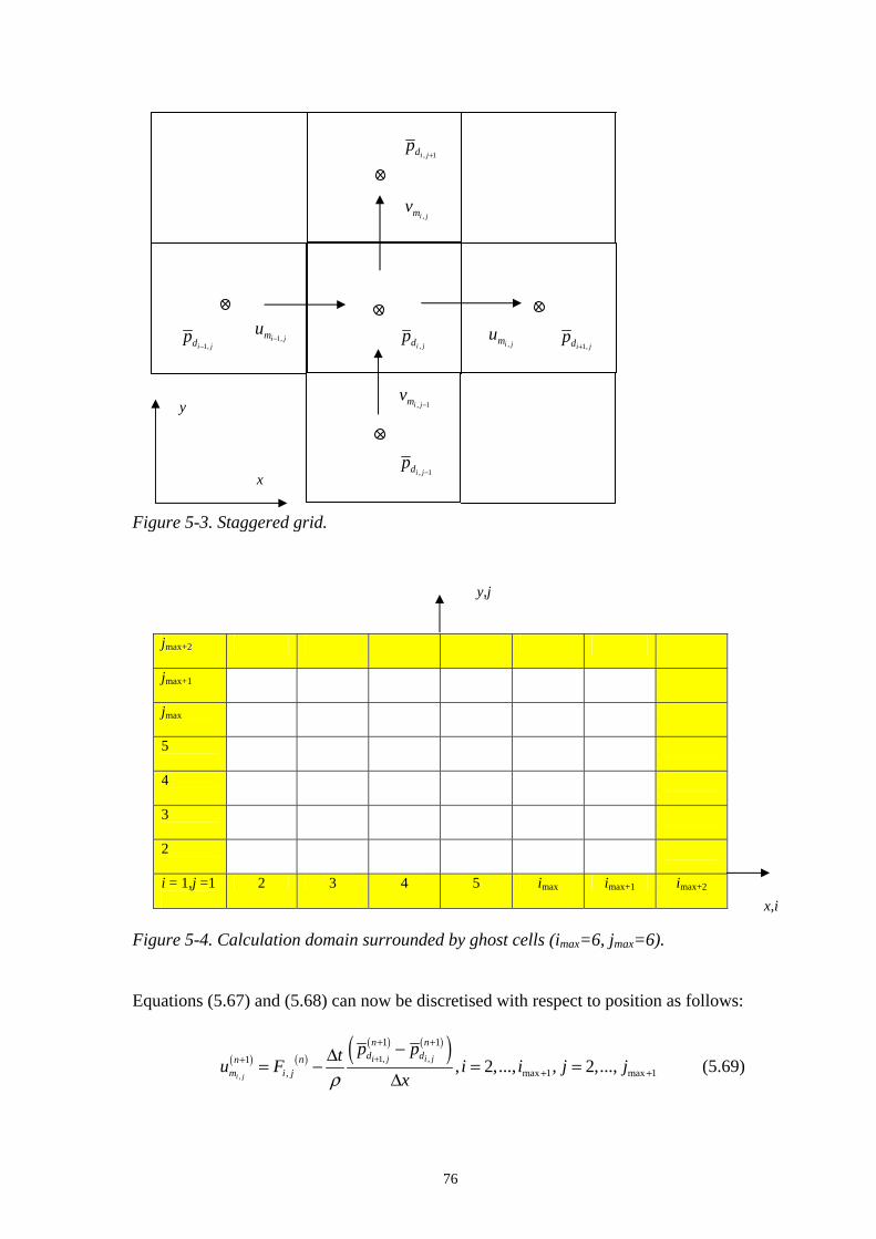
76

Figure 5-3. Staggered grid.

jjmmaaxx++22

jmax+1

jmax

5

4

3

2

i = 1,j =1

2 3 4 5 imax imax+1 imax+2

Figure 5-4. Calculation domain surrounded by ghost cells (imax=6, jmax=6). Equations (5.67) and (5.68) can now be discretised with respect to position as follows:

( ) ( )( ) ( )( )

,

,1,

1 1

1, max 1 max 1, 2,..., , 2,...,

i j

i ji j

n nd dnn

m i j

p ptu F i i j jxρ

+

+ +

++ +

−Δ= − = =Δ

(5.69)

x,i

y,j

,i jdp ,i jmu 1,i jmu

−

, 1i jmv−

,i jmv

1,i jdp+

1,i jdp

−

, 1i jdp−

, 1i jdp+

y

x

77

( ) ( )( ) ( )( )

,

,1,

1 1

1, max 1 max 1, 2,..., , 2,...,

i j

i ji j

n nd dnn

m i j

p ptv G i i j jyρ

+

+ +

++ +

−Δ= − = =Δ

, (5.70)

where F and G are discretised at the right and upper walls of the cells, respectively, in the same fashion as the velocities. The spatial derivatives in F and G were calculated by replacing the first derivatives by centred differences and the second derivatives by donor cell discretisation. 5.3.2 Solution of the Poisson-type equation In order to solve pressure at the new time step, the continuity equation (5.44) is first written as follows:

0m mm m

u vh h hh u h vx x y y t

∂ ∂∂ ∂ ∂+ + + + =∂ ∂ ∂ ∂ ∂

. (5.71)

The velocity field ( ) ( )( )1 1,Tn n

m mu v+ + from Equations (5.67) and (5.68) is now inserted into

Equation (5.71) and the following Poisson-type equation can be written:

( ) ( ) ( ) ( )1 1 1 12 2

2 2

n n n n

d d d dp p p ph hh hx y x x y y

+ + + +

∂ ∂ ∂ ∂∂ ∂+ + + =∂ ∂ ∂ ∂ ∂ ∂

( ) ( )

( ) ( )n n

n nF G h h hh h F Gt x y x y t

ρ ⎛ ⎞∂ ∂ ∂ ∂ ∂+ + + +⎜ ⎟⎜ ⎟Δ ∂ ∂ ∂ ∂ ∂⎝ ⎠. (5.72)

The Poisson-type equation can now be discretised, which results in the following set of linear equations, which have imax ⋅ jmax unknown values of

,

( 1)i j

ndp + , i = 1,…,imax, j =

2,…,jmax, which have to be solved using a suitable iterative algorithm, such as the Gauss-Seidel method:

, , , , 1 , 1, 11, , 1, ,

( 1) ( 1) ( 1) ( 1) ( 1),i j i j i j i j i j ji j i j i j i j

n n n n nW d P d E d N d S d i jA p A p A p A p A p B

+ −− +

+ + + + ++ + + + = , (5.73)

where the compass notation has been applied for the coefficients A:

, , 1, , , , , 1,

, , ,2 2 2 2 2 2

2 2, ,

2 2i j i j i j i j i j i j i j i j

i j i j i j

n n n n n n nnc

W P Eu u c c c u u

h h h h h h hhA A A

x x x y x x− −

− −= − = − − = +

Δ Δ Δ Δ Δ Δ

, , , 1 , , , 1

, ,2 2 2 2, and2 2

i j i j i j i j i j i j

i j i j

n n n n n n

N Sc v v c v v

h h h h h hA A

y y y y− −

− −= + = −

Δ Δ Δ Δ

78

( )

, ,

, 1, , 1, , ,

, 1, , , 1,

1, 1, , , 1 ,

2 2

i j i j

i j i j i j i j i j i j

n n n ni j i j i j i jn n

i j

n n n n n nn n n nc ci j i j i j i j

c c

u u v v

F F G GB h h

t x y

h h h h h hF F G Gt x y t

ρ

ρ − −

− −

+− −

⎛ ⎞− −= + +⎜ ⎟⎜ ⎟Δ Δ Δ⎝ ⎠⎛ ⎞− − −− −⎜ ⎟+ +⎜ ⎟Δ Δ Δ Δ⎝ ⎠

where the subscripts in , and c u vh h h indicate that the height of the gap is calculated at the centre of the cell, at the right-hand edge of the cell, and at the upper edge of the cell, respectively. The iterative solution of the equations in (5.73) is called the inner iteration. Patankar's under-relaxation was adopted in order to improve the convergence of the inner iteration (see e.g. Ferziger and Peric (2002), pp. 118-119). Normally, under-relaxation of the pressure is performed as follows: ( ), , , ,

( 1)i j i j i j i j

n n new nd d p d dp p p pα+ = + − , (5.74)

where pα is the under-relaxation factor for pressure, satisfying 0 1pα< < , and

,i j

newdp

is the solution for the pressure in cell i,j from Equation (5.73). Now, solving ,

( 1)i j

ndp +

from Equation (5.73) and inserting it into Equation (5.74) in place of ,i j

newdp , Equation

(5.74) was re-written as follows:

,

, , , 1 , 1 ,1, , 1, , , ,

* *, ,

( 1) ( 1) ( 1) ( 1) ( 1),

1i j

i j i j i j i j i ji j i j i j i j i j i j

Pi j i j

P pn n n n n nW d d E d N d S d i j P d

p p

A B

AA p p A p A p A p B A p

αα α+ −− +

+ + + + + −+ + + + = + (5.75)

where

,

*i jpA are modified main diagonal matrix elements and *

,i jB are modified source vector components. This modified equation is solved within inner iterations. When the outer iterations converge, the terms involving pα cancel each other out, since

, ,

( 1)i j i j

n nd dp p+ → , and the solution of the original problem (5.73) will be obtained.

Patankar's under-relaxation was found to have a very positive effect on the convergence of the iterative solution method, because the diagonal dominance of the matrix A is increased. 5.3.3 The outer iteration After the pressure in the cells of the calculation domain has been obtained at the new time step tn+1, the new values for the velocity components ( )

,

1

i j

n

mu + and ( ),

1

i j

n

mv + can be obtained by using the discretised equations of motion (5.69) and (5.70). Under-relaxation was used in the outer iteration for calculation of the velocities: ( ), , , ,

( 1)i j i j i j i j

n n new nm m m mu u u uα+ = + − (5.76)

and

79

( ), , , ,

( 1)i j i j i j i j

n n new nm m m mv v v vα+ = + − , (5.77)

where α is the under-relaxation factor for the velocities in the x- and y-coordinate directions and

, ,and

i j i j

new newm mu v are obtained from Equations (5.69) and (5.70).

The outer iteration, i.e. the (n + 1)st time step, consists of the following steps: 1. Compute F(n) and G(n) according to (5.65) and (5.66) using velocities ( )n

mu and ( )nmv .

2. Solve the Poisson-type equation (5.72) for the pressure ( )1n

dp + . 3. Compute the new velocity field ( ( 1) ( 1),n n

m mu v+ + )T using Equations (5.76) and (5.77) with the pressure values, ( 1)n

dp + , obtained in Step 2. The outer iteration now continues until a preset value for the L2 norm of the change of velocity between iteration cycles has been achieved. The L2 norm is defined as:

( )max max

1/ 22

, 21 1max max

1 i jit it

i ji j

r ri j = =

⎛ ⎞= ⎜ ⎟⎝ ⎠

∑∑ , (5.78)

where ,

iti jr is the change of velocity in the x-coordinate direction,

, ,

( 1) ( )

i j i j

n nm mu u+ − ,

between the successive iteration cycles. 5.3.4 The boundary conditions The iteration process described above gives the solution for the variables in the cells of the calculation domain (i = 2 to imax+1, j = 2 to jmax+1; see Figure 5-4). For the cells outside the calculation domain, i.e. for the ghost cells, values for the variables

, and m m du v p either have to be given or be determined on the basis of the values of the respective variables in the calculation domain. The no-slip, symmetric, periodic, inflow, outflow, free flow, and dynamic boundary conditions were used in this study. 5.3.4.1 No-slip boundary condition The no-slip boundary condition means that the mean velocities should vanish at a fixed boundary to satisfy the no-slip condition: 0, 0n tφ φ= = , (5.79) where nφ denotes the velocity normal to the wall and tφ the velocity tangential to the wall. This boundary condition was used at the boundaries of obstacle cells, where no fluid motion was assumed to exist, and the calculation domain. The obstacle cells were defined in areas where contact between the hull and the ice floe was assumed to exist.

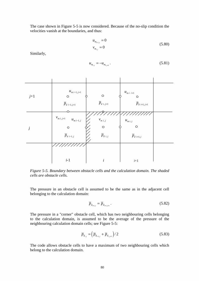
80

The case shown in Figure 5-5 is now considered. Because of the no-slip condition the velocities vanish at the boundaries, and thus:

1,

,

0

0i j

i j

m

m

u

v−

=

= (5.80)

Similarly,

, , 1i j i jm mu u+

= − . (5.81) Figure 5-5. Boundary between obstacle cells and the calculation domain. The shaded cells are obstacle cells. The pressure in an obstacle cell is assumed to be the same as in the adjacent cell belonging to the calculation domain:

1, 1, 1i j i jd dp p+ + +

= . (5.82) The pressure in a "corner" obstacle cell, which has two neighbouring cells belonging to the calculation domain, is assumed to be the average of the pressure of the neighbouring calculation domain cells; see Figure 5-5: ( ), 1, , 1

/ 2i j i j i jd d dp p p

− += + (5.83)

The code allows obstacle cells to have a maximum of two neighbouring cells which belong to the calculation domain.

,d i jp 1,d i jp −

, 1d i jp + 1, 1d i jp − +

m 1, 1i ju − +

m 1,i ju −m , 1i jv +

,m i jv m ,i ju

m , 1i ju +

i-1 i

j

j+1

i+1

1,d i jp +

1, 1d i jp + +

81

5.3.4.2 Symmetric or free-slip boundary condition The symmetric or free-slip boundary condition prevents fluid flow through the boundary, but, contrary to the no-slip boundary condition, there are no frictional losses at the boundary: 0, / 0, / 0n t dn p nφ φ= ∂ ∂ = ∂ ∂ = . (5.84) The symmetric boundary condition or free-slip boundary condition can be assigned e.g. for the southern edge of the calculation domain shown in Figure 5-4 by setting:

,1 ,2

,10,

i i

i

m m

m

u u

v

=

= (5.85)

and by setting the following values for the coefficients of the Poisson equation in the ghost cells at the southern edge:

,1 ,1 ,1

,1

,1

,1 0

1

1,

i i i

i

i

W E S i

P

N

A A A B

A

A

= = = =

=

= −

(5.86)

a symmetric pressure field at the southern edge will be obtained, i.e. ,1 ,2.d di ip p= (5.87) 5.3.4.3 Periodic boundary condition For problems which have a periodic geometry with a period l in one coordinate direction, the computations can be restricted to one period. The velocities and pressure must then coincide at the opposite boundaries, for example for a periodic flow in the x-coordinate direction (see Figure 5-4):

( ) ( ) ( ) ( ) ( ) ( )/ 2, / 2, , / 2, / 2, , / 2, / 2,n n t t d dl y l y l y l y p l y p l yφ φ φ φ− = − = − = . (5.88) where the length of the period is l. The periodic boundary condition can be assigned e.g. for the western edge of the calculation domain shown in Figure 5-4 by setting:

1, max 1,

1, max 1,,

j i j

j i j

m m

m m

u u

v v+

+

=

= (5.89)

and by setting the coefficients of the Poisson equation in the ghost cells:

82

1, 1, 1,

1,

1,

1, 0

1

0.5,

j j j

j

j

W N S j

E

P

A A A B

A

A

= = = =

=

=

(5.90)

and by connecting the pressures in Gauss-Seidel iteration when solving the Poisson-type equations: 1, max 1,j d i jB p += , (5.91) a periodic pressure field between the left- and right-hand edges will be obtained, i.e.: 1, max 1,d dj i jp p += . (5.92) 5.3.4.4 Inflow and outflow boundary conditions The inflow boundary condition at the inlet can be set by giving both velocity components (see e.g. Griebel et al. (1998)), but in this study the inflow boundary condition was set in such a way that the velocity in the x-coordinate direction at the inlet or outlet surfaces was calculated from the control volumes of the cells bordering the inlet and outlet inside the calculation domain and the velocity in the y-coordinate direction at the inlet or outlet was assumed to be zero, in a similar fashion as was done by Leschziner (1976):

( ) ( )1, 2, 2, 2, 1 2, 1 2, 2,

2, 2, 1,

1, 2, 2, 1,

( ) ( 1)

[

+ / ] /

/

j j j j j j j

j j j

j j j j

m m u m v m v

n nc c u

m m v v

u u h y v h x v h x

h h t x y h y

v v h h

− −

−

= Δ − Δ + Δ

⎡ ⎤− Δ Δ Δ Δ⎣ ⎦= −

(5.93)

The last term of the first equation inside the square brackets takes into account the effect of possible change in the gap height with time on the velocity. The outflow boundary condition at the outlet was set in a similar way:

( ) ( )max 2, max 1, max 1, max 2, 1 max 2, 1 max 2, max 2,

max 2, max 2, max 2,

max 2, max 1, max 1, max 2,

( ) ( 1)

[

+ / ] /

/ .

i j i j i j i j i j i j i j

i j i j i j

i j i j i j i j

m m u m v m v

n nc c u

m m v v

u u h y v h x v h x

h h t x y h y

v v h h

+ + + + − + − + +

+ + +

+ + + +

−

= Δ − Δ + Δ

⎡ ⎤− Δ Δ Δ Δ⎣ ⎦= −

(5.94)

The magnitude of pressure at the inlet or outlet has to be given, if inflow or outflow boundary condition is used. 5.3.4.5 Free-flow boundary condition The free-flow boundary condition means that the velocity does not change in the direction normal to the boundary and the pressure is given, being e.g. zero:

83

/ 0, / 0, 0n t dn n pφ φ∂ ∂ = ∂ ∂ = = . (5.95) Assuming that the purpose is to assign the free-flow boundary condition at the northern edge in Figure 5-4, it can be written:

( )

( )

0

0.

m u

m v

u hy

v hy

∂=

∂∂

=∂

(5.96)

After the discretisation of the equations in (5.96) the velocities of the flow in the ghost cells are:

, max 2 , max 1 , max 1 , max 2

, max 2 , max 1 , max 1 , max 2

/

/ ,i j i j i j i j

i j i j i j i j

m m u u

m m v v

u u h h

v v h h+ + + +

+ + + +

= ⋅

= ⋅ (5.97)

where and u vh h mean the height of the right-hand and upper edges of the cells, respectively. The pressure can be assigned a zero value at the boundary by setting:

, max 2 , max 2 , max 2

, max 2 , max 1

, max 2 , max 1

, max 2 0

.

i j i j i j

i j i j

i j i j

W E N i j

P P

S P

A A A B

A A

A A

+ + +

+ +

+ +

+= = = =

=

=

(5.98)

Inserting the coefficients (5.98) into the Poisson equation (5.73) gives: , max 2 , max 1d di j i jp p+ += − , (5.99) indicating that the pressure is zero at the upper edge of the calculation domain. 5.3.4.6 Dynamic boundary condition The dynamic boundary condition is a special boundary condition which was only used at the northern edge of the calculation domain. The idea is to allow some fluid flow through the gap between the adjacent ice floes at the northern edge. For the sake of simplicity, the flow through the gap between the ice floes was modelled as a stationary laminar flow between two parallel walls, as depicted in Figure 5-6. It is also assumed that the gaps between the ice floes and the hull are symmetrical relative to the z-axis, see Figure 5-6. The flow in the gap between the ice floes is driven by the pressure difference

1 2dp p pΔ = − between the lower and upper ends of the gap. The pressure difference can be obtained from Equation (5.6) by setting h = δ , U = 0, kx = 12,

, m mx z u w→ → and / /d d icedp dx p h→ Δ :

84

2

12 iced m

hp wηδ

Δ = − , (5.100)

where hice is the ice thickness, δ is the width of the gap, and wm is the average velocity of the flow in the gap between the edges of the ice floes. Assuming that the flow in or out from the gap between the hull surface and the ice floe is generated only by the flow in the y-coordinate direction, it can be written on the basis of the continuity equation:

, max 1 , max 12 i j i jm m vw v hδ

+ += , (5.101)

Figure 5-6. Flow in the gap between two adjacent ice floes at the northern edge of the calculation domain. where

, max 1i jmv+

is the velocity of the flow in the y-coordinate direction in Cell (i,jmax+1)

at the northern edge of the calculation domain, and , 1i jmaxvh

+ is the height of that cell.

Assuming 1 i,jmax+1dp p= , and further assuming p2 = 0 results in the following boundary condition for the velocity in the y-coordinate direction at the northern edge:

, max 1

, max 1

, max 1

3

24i j

i j

i j

dm

ice v

pv

h h

δη

+

+

+

= . (5.102)

hice

δ

p1

p2=0

vm (i,jmax+1)

Ice floe

hull surface

wm

vm (i,jmax+1)

Ice floe

y

z

( )i,jmax 1dp +

85

The other boundary conditions at the northern edge are:

, max 2 , 1

, max 2 , max 1.

i j i jmax

i j i j

m m

d d

u u

p p+ +

+ +

=

= (5.103)

5.3.5 Numerical stability of the solution method Stability conditions must be imposed on the step sizes , and x y tΔ Δ Δ , in order to ensure stability and avoid generating oscillations in the iteration process. In the Iceflo computer code the Courant-Friedrichs-Levy (CFL) conditions were used (see e.g. Griebel et al. (1998)), which state that no fluid particle may travel a distance greater than the mesh spacing xΔ or yΔ in time tΔ :

max maxm m

, x yt tu vΔ ΔΔ < Δ < , (5.104)

where

max maxm m and u v are the maximal absolute values of the velocities occurring in the cells of the calculation domain. An adaptive step size control may be used by selecting tΔ for the next time step so that each of the two conditions (5.104) is satisfied:

max maxm m

: min , ,fx yt S

u v

⎡ ⎤Δ Δ⎢ ⎥Δ =⎢ ⎥⎣ ⎦

(5.105)

where the factor Sf is a safety factor ( )0 1fS< ≤ . A constant time step based on the speed of the upper wall and an adaptive time step based on the actual velocities in the cells of the calculation domain were implemented in Iceflo. 5.4 Calculation of forces and moment resulting from pressure and shear

stress Assuming that the hull surface moves in the x-direction (see Figure 3-2) the expression for the shearing stress, wτ , on the surfaces under laminar flow conditions is:

1,2 2

dw

pU hh x

ητ ∂= ±∂

, (5.106)

where the subscripts 1 and 2 refer to the upper and lower walls, respectively. It can be seen that for laminar plane Couette flow Equation (5.106) gives a constant shear stress

1,2/w U hτ η= .

86

Constantinescu and Galetuse (1965) and (1974) have shown, employing the mixing length theory, that the shearing stresses under turbulent flow acting on the wall surfaces depend on the Couette Reynolds number and on the pressure gradient, as follows:

( )1,2

0.941 0.0012 2Re2

dw C

pU hh x

ητ ∂⎡ ⎤= + ±⎣ ⎦ ∂ (5.107)

The total shear force acting on the ice floe or the hull surface is obtained by integrating Expression (5.106) or (5.107) numerically over the area of the ice floe. The average pressure change in the gap between the hull surface and the ice floe,

1dp , is obtained by summing the values of pressure in the cells of the calculation domain obtained from Equation (5.75) and dividing the sum by the total number of cells. The total normal force resulting from the pressure in the gap acting on the ice floe or the hull surface is obtained by multiplying the average pressure change in the gap with the area of the ice floe. The moment around the y-axis acting on the ice floe due to asymmetric pressure field in the gap between the hull surface and the ice floe is calculated by summing over the calculation domain the force due to pressure in each cell multiplied by the distance from the centre of the cell to the y-axis. Moment acting in a clockwise direction is defined to have a positive sign. 5.5 Verification and validation of the Iceflo CFD code In this section the Iceflo CFD code is verified for two-dimensional flow against the results obtained using the analytical solution given by Constantinescu and Galetuse (1974) for a flow between a transversely infinite rotating cylinder and an infinite wall. For three-dimensional flow the Iceflo CFD program was verified and validated against the analytical solution of Kapitsa (see Cameron (1976)) for a flow between an egg-shaped hull moving above a plane. Validation of Iceflo for a time-dependent flow, i.e. for a flow with changing gap height, could be performed for the analytical solution of two infinitely wide parallel walls approaching or moving away from each other, i.e. for a pure squeeze film lubrication case. 5.5.1 Verification of Iceflo against the analytical solution of Constantinescu

for a two-dimensional flow between a rotating cylinder and an infinite wall

As an example, a steady two-dimensional flow in the gap between a circular wall at z = h(x), rotating with a tangential speed, U, and a flat stationary wall at z = 0, is considered, as depicted in Figure 5-7. It is assumed that the radius of curvature of the rotating wall is large compared to the length of the stationary wall l, and thus at the upper wall the velocity of the wall surface in the x-coordinate direction is approximately the same as the tangential speed, U. The minimum distance between the walls is hmin in the middle of the gap at x = 0. The fluid between the walls is water,

87

T = 0 oC, ρ = 1000 kg/m3, and 31.792 10 Pa sη −= ⋅ ⋅ . Periodic boundary conditions are assumed at the ends of the channel between the walls. Figure 5-7. The geometry of the gap between a rotating cylinder and a stationary flat wall. For a steady two-dimensional flow, for example for a flow between a transversely infinite rotating cylinder and an infinite wall, the global momentum equations (5.42) and (5.43) and the continuity equation (5.44) reduce to:

( )2 2 02

d xm m m

p k Uu h U h u Uh h ux x h

ηρ α β γ ∂∂ ⎛ ⎞+ − + + − =⎜ ⎟∂ ∂ ⎝ ⎠ (5.108)

mu h Q= , (5.109) where Q is the constant rate of flow in the gap. These give:

2 2

2 3

212

d xdp k U Q Q dh U dhdx h Uh h dx h dx

η αρ βρ⎛ ⎞= − + −⎜ ⎟⎝ ⎠

, (5.110)

where 1.2 and 0.133α β= = for laminar flow (see the equations in (5.45)). For turbulent flow the pressure equation takes a slightly different form, in which

1 and α β= is considered as being related to the local Couette Reynolds number, ( )ReC x ; see the equations in (5.46):

2 2

2 3

21 0.6332

d xdp k U Q Q dh U dhdx h Uh h dx h dx

η ρ βρ⎛ ⎞= − + −⎜ ⎟⎝ ⎠

. (5.111)

The pressure distribution in the gap can now be calculated by integrating Equation (5.110) in the case of laminar flow and Equation (5.111) in the case of turbulent flow and using appropriate boundary conditions at the ends of the gap. Assuming the pressure to be zero at both ends of the gap, the following expression can be obtained for the flow rate in the gap for turbulent flow (see Constantinescu and Galetuse (1974)):

Stationary wall, u = 0 x

Outlet Inlet

-l/2 l/2

minh

h(x) z

Rotating wall

U

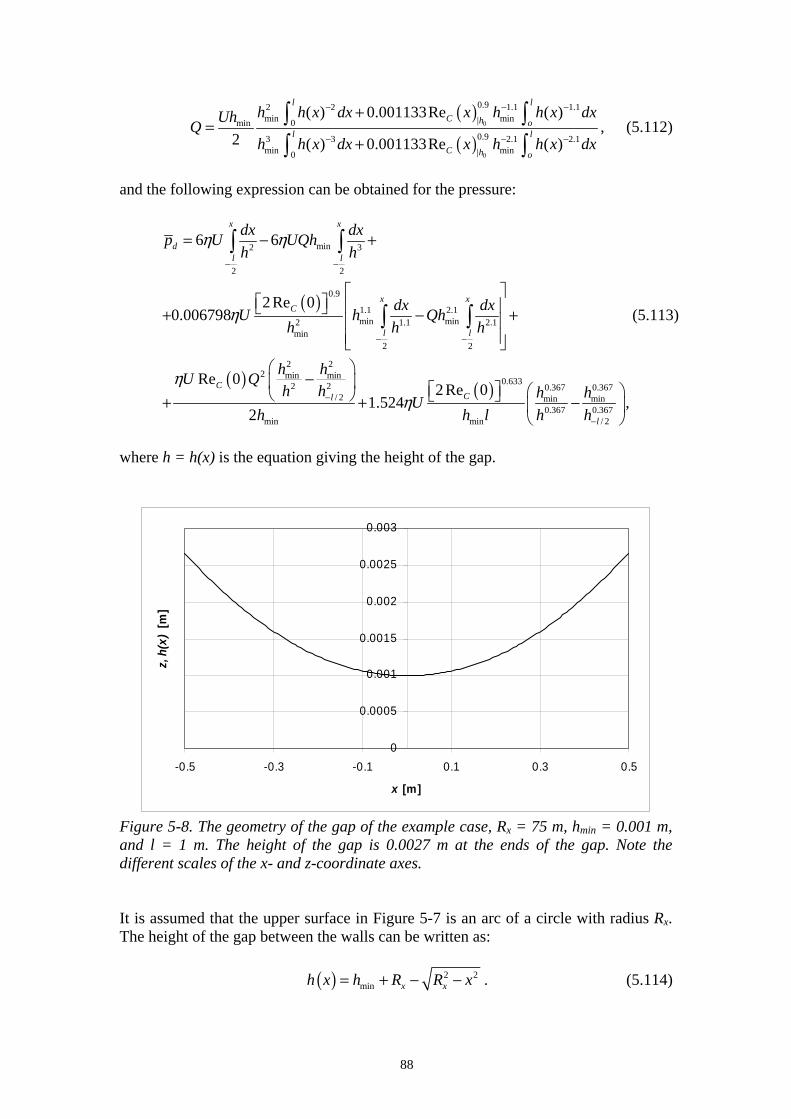
88

( )( )

0

0

0.92 2 1.1 1.1min min| 0 min

0.93 3 2.1 2.1min min| 0

( ) 0.001133Re ( )

2 ( ) 0.001133Re ( )

l l

C h ol l

C h o

h h x dx x h h x dxUhQh h x dx x h h x dx

− − −

− − −

+=

+

∫ ∫∫ ∫

, (5.112)

and the following expression can be obtained for the pressure:

( )

( ) ( )

min2 3

2 2

0.9

1.1 2.1min min2 1.1 2.1

min2 2

2 22 min min 0.6332 2 0.367 0.3

/ 2 min min0.367

min min

6 6

2Re 00.006798

Re 02Re 0

1.5242

x x

dl l

x xC

l l

CCl

dx dxp U UQhh h

dx dxU h Qhh h h

h hU Qh h h hU

h h l h

η η

η

ηη

− −

− −

−

= − +

⎡ ⎤⎡ ⎤ ⎢ ⎥⎣ ⎦+ − +⎢ ⎥

⎢ ⎥⎣ ⎦⎛ ⎞

−⎜ ⎟ ⎡ ⎤⎝ ⎠ ⎣ ⎦+ + −

∫ ∫

∫ ∫

67

0.367/ 2

,lh−

⎛ ⎞⎜ ⎟⎝ ⎠

(5.113)

where h = h(x) is the equation giving the height of the gap.

0

0.0005

0.001

0.0015

0.002

0.0025

0.003

-0.5 -0.3 -0.1 0.1 0.3 0.5

x [m]

z, h

(x)

[m]

Figure 5-8. The geometry of the gap of the example case, Rx = 75 m, hmin = 0.001 m, and l = 1 m. The height of the gap is 0.0027 m at the ends of the gap. Note the different scales of the x- and z-coordinate axes. It is assumed that the upper surface in Figure 5-7 is an arc of a circle with radius Rx. The height of the gap between the walls can be written as: ( ) 2 2

min x xh x h R R x= + - - . (5.114)

89

The geometry of the gap is depicted in Figure 5-8, when Rx = 75 m, l = 1 m and hmin = 0.001 m using a distorted scale. The pressure distribution in the gap obtained by Iceflo is compared with the results obtained by the analytical solution of Constantinescu for laminar flow in Figure 5-9 and for turbulent flow in Figure 5-10. For turbulent flow the turbulence model of Constantinescu was used (see the first expression (5.47)). The analytical solution was obtained from Equations (5.112) and (5.113). The results of Iceflo are compared with the results obtained by the analytical solution in Tables 5-2 and 5-3. In both cases the numerical solution coincides very well with the analytical solution. It may also be noted that, as a result of inertia effects, in both cases the average pressure in the gap is negative.

-400

-300

-200

-100

0

100

200

300

-0.6 -0.4 -0.2 0 0.2 0.4 0.6

x [m]

Pres

sure

[Pa]

IcefloAnalytical solution

Figure 5-9. Comparison of the results of Iceflo with the analytical solution of Constantinescu. Laminar flow, ReC = 279 - 744, U = 1 m/s.

-8000

-6000

-4000

-2000

0

2000

4000

-0.6 -0.4 -0.2 0 0.2 0.4 0.6

x [m]

Pres

sure

[Pa]

IcefloAnalytical solution

Figure 5-10. Comparison of the results of Iceflo with the analytical solution of Constantinescu. Turbulent flow, ReC = 1395 - 3720, U = 5 m/s.

90

Table 5-2. Comparison of the analytical solution with the results of Iceflo (laminar flow). Mass flow [kg/sm] Average shear

stress [N/m2] Average pressure [Pa]

Analytical solution 0.613 1.035 -12.2 Iceflo 0.613 1.034 -12.8

Table 5-3. Comparison of the analytical solution with the results of Iceflo (turbulent flow). Mass flow [kg/sm] Average shear


Analytical solution 3.178 20.538 -1660 Iceflo 3.179 20.526 -1653

5.5.2 Validation of Iceflo against Fluent for two-dimensional flow The Iceflo computer code was verified against Fluent for a steady flow between a transversely infinite rotating cylinder and an infinite wall (see Figure 5-7). The lower wall is steady, the upper wall is rotating with a tangential speed of U, the left-hand wall is the inlet, and the right-hand wall is the outlet. Periodic boundary conditions were used between the inlet and the outlet. The length of the lower wall, l, is 1.0 m, the radius of curvature of the upper wall, R, is 75 m, and the minimum distance between the walls, hmin is 0.001 m (see Figure 5-8). Table 5-4. The 149x39 low Reynolds number grid. Direction Number

of cells Length of the first and the last cell [m]

Length of the cell in the middle [m]


x (-0.5 m to 0.5 m) 149 0.006711409 0.006711409 1 z (0 m to 0.001666685 m) 39 0.000004444 0.00022 1.18

The fluid between the walls is water, T = 0 oC, ρ = 1000 kg/m3, and

31.792 10 Pa sη −= ⋅ ⋅ . The k ε− turbulence model of Fluent with two-zonal wall treatment was used and therefore the dimensionless wall distance was required to be less than unity, / 1.z zut n+ = £ The height of the first cell in the z-coordinate direction was selected to be = 0.000004444 m.zD A 149x39 grid was generated, as shown in Table 5-4. The cell width-to-height ratio /x zΔ Δ thus varies from 1510 to 30.5.

91

5.5.2.1 Laminar flow The Iceflo computer code was run using the same geometry, the same boundary conditions, and a grid with 149 cells in the x-coordinate direction. The results of the calculation are shown in Table 5-5. Fluent gives a larger average pressure decrease in the gap than Iceflo. Table 5-5. Comparison of the numerical solutions of Fluent and Iceflo (laminar flow). Mass flow [kg/sm] Average shear


Fluent 0.613 1.036 -21.4 Iceflo 0.613 1.034 -12.8

Figure 5-11. Velocity vectors at three sections near the inlet. The velocity vectors at the inlet calculated by Fluent are depicted in Figure 5-11. It should be noted that backflow exists at the inlet. According to Equation (5.51), flow film separation should occur at the point where um = U/3. According to the results obtained by Iceflo, it occurs at about 0.36 x m= ± in this case. This result is in line with the results obtained by Fluent. The pressure distribution in the gap obtained by Fluent and Iceflo for laminar flow is shown in Figure 5-12.

92

-400

-300

-200

-100

0

100

200

300

-0.6 -0.4 -0.2 0 0.2 0.4 0.6

x [m]

Pres

sure

[Pa]

IcefloFluent

Figure 5-12. Comparison of the pressure distribution in the gap obtained by Iceflo and Fluent. Laminar flow, ReC = 279 - 744, U = 1 m/s. 5.5.2.2 Turbulent flow A double-precision, two-dimensional version of Fluent with a segregated and implicit solver was used. In Fluent standard treatment of pressure, using the SIMPLE method for pressure-velocity coupling, was selected. Second-order upwind was selected for the discretisation of the momentum, k and ε equations. The results of the calculations are shown in Table 5-6. Fluent gives a higher average pressure decrease in the gap than Iceflo. Table 5-6. Comparison of the numerical solutions of Fluent and Iceflo (turbulent flow). Mass flow [kg/sm] Average shear


Fluent 3.191 22.778 -2009 Iceflo 3.179 20.526 -1653

The velocity vectors at the inlet calculated by Fluent are depicted in Figure 5-13. It should be noted that there is no backflow at the inlet. The calculations made using Equation (5.57), however, indicate that backflow should occur. Therefore the use of Equation (5.57) does not seem to be relevant for backflow analysis. Correct results could be obtained using Equation (5.58), when a value of 7.45 was used for Hs (see Section 5.2.6). The Iceflo computer code was run using the same geometry, the same boundary conditions, and a grid with 149 cells in the x-coordinate direction. The turbulence model of Costantinescu was used in the calculations. The results of the calculation are shown in Table 5-6. The pressure distributions in the gap obtained by Fluent and Iceflo for turbulent flow are shown in Figure 5-14 (U = 5 m/s). As in the case of

93

laminar flow, a slight difference between the results of Iceflo and Fluent can be observed. The reason for this may not be due to the different kinds of turbulence models used in Iceflo and Fluent, because the same trend can also be observed in the laminar case. The reason for this difference may thus be due to the simplifications made in the derivation of Equations (5.42) and (5.43).

Figure 5-13. Velocity vectors at two sections near the inlet.

-8000

-6000

-4000

-2000

0

2000

4000

-0.6 -0.4 -0.2 0 0.2 0.4 0.6

x [m]

Pres

sure

[Pa]

IcefloFluent

Figure 5-14. Comparison of the results of Iceflo with Fluent. Turbulent flow, ReC = 1395 - 3720, U = 5 m/s.

94

5.5.3 Validation of Iceflo for a three-dimensional flow An egg-shaped hull moving at a speed U above a plane is now considered. The flow is assumed to be laminar and steady and thus 12x yk k= = . Let the minimum distance between the hull and the plane be minh , and the hull have radii and x yR R in the x- and y-coordinate directions. Then

2 2

min 2 2x y

x yh hR R

≈ + + . (5.115)

Assuming further that the inertia effects are negligible, a solution for Equation (5.4) is sought. Put as the trial solution 2/dp kx h= , where k is some as yet unknown constant. The first and the second terms in Equation (5.4) can now be written:

3

3

312 12

.12 6

d

x

d

y

ph kxx x R

ph kxy y R

η η

η η

⎛ ⎞∂∂ = −⎜ ⎟∂ ∂⎝ ⎠⎛ ⎞∂∂ = −⎜ ⎟∂ ∂⎝ ⎠

(5.116)

With this trial solution Equation (5.4) now becomes:

312 6 2x y x

kx kx UxR R Rη η

− − = , (5.117)

so ( )6 / 3 2 /x yk U R Rη= − + , and hence:

( ) 2

63 2 /d

x y

U xpR R h

η= −+

. (5.118)

This first analytical solution of the Reynolds equation in three dimensions was derived by Kapitsa; see Cameron (1976). An example of the pressure distribution calculated according to Equation (5.118) is shown in Figure 5-15 for the flow in the gap between a ball-shaped hull and a plane. The following parameters were used in the calculation: l = 1 m, b = 1 m, Rx = 75 m, Ry = 75 m, hmin = 0.0001 m, U = 1.0 m/s, and 31.792 10 Pa sη −= ⋅ ⋅ for water. The pressure distribution in the section y = 0.005 m is shown in Figure 5-16 both for the analytical solution and for the numerical solution calculated using Iceflo. Iceflo was run with the pressure at the boundaries of the calculation domain set according to Equation (5.118). It can be seen that the numerical solution follows the analytical solution quite closely. It can also be observed that the pressure distribution in the gap is anti-symmetric and thus the average pressure in the gap is zero (compare with the results given in Section 5.5.1).

95

-0.5 -0.4 -0.3 -0.2 -0.1 0.0 0.1 0.2 0.3 0.4 0.50.5

0.0-10000

-8000

-6000

-4000

-2000

0

2000

4000

6000

8000

10000

Pres

sure

[Pa]

x [m]

y [m]

Figure 5-15. Pressure distribution in the gap, according to Kapitsa.

-8000

-6000

-4000

-2000

0

2000

4000

6000

8000

-0.6 -0.4 -0.2 0 0.2 0.4 0.6

x [m]

Pres

sure

[Pa]

IcefloKapitsa

Figure 5-16. Comparison of the results of Iceflo with the results of Kapitsa, pressure distribution in the section y = 0.005 m.

96

5.5.4 Validation of Iceflo against a flow generated by infinitely wide parallel walls approaching or moving apart

Let two parallel walls which are infinitely wide in the y-axis direction approach or move away from each other (compare with Cameron (1976), pp. 117-118); then, for laminar flow, the Reynolds equation (5.4) reduces to:

3 12dp dhhx x dt

η∂∂ ⎛ ⎞ =⎜ ⎟∂ ∂⎝ ⎠. (5.119)

Integrating twice yields:

21 23

/6ddh dtp x C x C

hη= + + . (5.120)

Zero pressure boundary conditions at the ends are used, p = 0 on x = ± l/2, when l is the length of the walls. Hence C1 = 0 and

2

2 3

6 /4

l dh dtCh

η= − , (5.121)

and

2

23

/64d

dh dt lp xh

η ⎛ ⎞= −⎜ ⎟

⎝ ⎠. (5.122)

For approaching walls /dh dt is negative, and thus there is a positive pressure between the walls. Correspondingly, the pressure is negative if the walls are moving apart and /dh dt is positive. An approximate solution of the above-mentioned problem can also be found for a laminar flow with inertia effects (see Pinkus and Sternlicht (1961)). Recalling Equation (5.14), the following equation for a two-dimensional steady laminar flow can be obtained:

( ) ( )2

2dp uuu wu

x z x zρ η∂∂ ∂ ∂⎡ ⎤+ = − +⎢ ⎥∂ ∂ ∂ ∂⎣ ⎦

. (5.123)

Using the same assumptions as in Section 5.2, Equation (5.123) is integrated across the film thickness, which results in:

2

20

1 hdpu u uu w dz

h x z x zρ η⎡ ⎤ ∂∂ ∂ ∂⎛ ⎞+ = − +⎢ ⎥⎜ ⎟∂ ∂ ∂ ∂⎝ ⎠⎣ ⎦∫ . (5.124)

By moving all the terms, which are a function of x alone, to the left-hand side of the equation, Equation (5.124) can be written as follows:

97

0

1 ( )h

dpu uu w dz f xh x z xρη η

∂∂ ∂⎛ ⎞+ + =⎜ ⎟∂ ∂ ∂⎝ ⎠∫ , (5.125)

where

2

2 ( )u f xz

∂ =∂

. (5.126)

Integrating Equation (5.126) twice yields: 2

1 2½ ( ) ( ) ( )u f x z C x z C x= + + . (5.127) By using the continuity equation / / 0u x w z∂ ∂ + ∂ ∂ = :

3 ' 2 '1 2 3

1 1'( ) ( ) ( ) ( )6 2

uw z f x z C x z C x z C xx

∂ ⎛ ⎞= − ∂ = − + + +⎜ ⎟∂ ⎝ ⎠∫ , (5.128)

where the primes denote differentiation with respect to x. The boundary conditions are:

0, 0 at 00, / at

0 at / 2 d

u w zu w dh dt z hp x l

= = == = =

= = ± (5.129)

Using the boundary conditions for velocities in the equations in (5.129):

( )43 3

12 / 12( )dh dt x

f x Ch h

= − , (5.130)

where C4 is an integration constant. Inserting f(x) into Equation (5.125) and using the boundary conditions for pressure in the equations in (5.129), the following equation for the pressure in the gap can be obtained from Equation (5.125):

2

23

6( / ) ( / )( )5 4d

dh dt dh dt h lp x xh

ρη ⎛ ⎞⎛ ⎞= − −⎜ ⎟⎜ ⎟⎝ ⎠⎝ ⎠

(5.131)

Equation (5.131) differs from Equation (5.122) obtained from the Reynolds equation by the supplementary term ( )/ / 5dh dt hρ− , which does not depend on the viscosity but which contains the density. Its effect on the pressure in the gap is proportional to the velocity of the upper wall and the distance between the walls. For approaching walls /dh dt is negative, there is overpressure between the walls, and the inertia term increases the pressure in the gap. If the walls are moving away from each other,

/dh dt is positive, there is negative pressure between the walls, and the inertia term again increases the pressure in the gap.

98

An example of pressure distribution in the gap between two infinitely wide parallel walls is given in Figure 5-17. The distance between the walls, h, was assumed to increase from 0.0009 m to 0.001 m in 0.2 s, and thus / 0.0005dh dt = m/s. The length of the parallel walls, l, was 1 m and the fluid was water with 31.792 10 Pa sη −= ⋅ ⋅ . The analytical solutions calculated using Equations (5.122) and (5.131) are compared with the results of Iceflo in Table 5-7 and in Figure 5-17. The results obtained by Iceflo coincide very well with the analytical solutions. Table 5-7. Comparison of the numerical solutions of Iceflo with analytical solutions.

Average pressure between the walls [Pa]

Analytical, without inertia effects -895.6 Iceflo, without inertia effects -910.0 Analytical, with inertia effects -845.7 Iceflo, with inertia effects -841.4

-1600

-1400

-1200

-1000

-800

-600

-400

-200

0

200

-0.5 -0.3 -0.1 0.1 0.3 0.5

x [m]

Pres

sure

[Pa]

Analytical, without inertia Analytical, with inertiaIceflo, without inertia Iceflo, with inertia

Figure 5-17. Pressure distribution between two infinitely wide walls moving away from each other, hmin = 0.001 m. This analysis also tells us that a high negative pressure between the walls is generated if the gap is small enough and the walls are moving away from each other. A greater distance between the walls gives much smaller values for the average force on the lower wall as a result of the negative pressure in the gap between the walls, as can be seen in Figure 5-18.

99

0.1

1

10

100

1000

10000

100000

1000000

0.0001 0.001 0.01

Distance between the walls, h [m]

Ave

rage

forc

e [N

/m]

Figure 5-18. Vertical force resulting from pressure on the lower wall when two infinitely wide walls are moving away from each other. Calculations were made using Equation (5.122), hmin ranges from 0.0001 m to 0.01 m. 5.6 Summary of Chapter 5 In this chapter the hydrodynamic lubrication theory for a three-dimensional flow with and without inertia effects was introduced. The Iceflo CFD code was written to calculate the flow in the gap between the hull surface and an ice floe. Iceflo was verified for a two-dimensional flow against the results calculated by the analytical solution derived by Constantinescu and Galetuse (1974) and validated against the results calculated by the Fluent computer code for a flow between an infinite rotating cylinder and a transversely infinite wall. The code was also verified for a three-dimensional flow against the analytical solution of Kapitsa for the flow between an egg-shaped hull and a plane that it was moving above. Verification and validation of Iceflo for a time-dependent flow, i.e. for a flow in a gap with changing gap height with time, were performed for the analytical solution of two, in a transverse direction, infinitely wide parallel walls approaching or moving away from each other. This analysis also indicated that a high negative pressure between the walls is generated if the gap is small enough and the walls are moving apart. In all cases the calculated results obtained with Iceflo coincided very well with the analytical solutions and reasonably well with the results obtained by Fluent.

100

6 Theoretical calculations In Section 1.8 the main goal of this study was set as being to study the effect of the following two phenomena on ice resistance in the sliding phase:

- the acceleration of water in the shear layer in the gap between the ice floe and the hull surface, and

- the flow of water to and from the shear layer resulting from changes in the geometry of the hull along the trajectory of an ice floe sliding against the hull.

In Section 6.1 the first phenomenon is analysed and in Section 6.2 the second one. The effect of the negative pressure in the gap between the hull surface and an ice floe on ice resistance due to the sliding phase is evaluated in Section 6.3. A summary of the analysis performed in Chapter 6 is presented in Section 6.4. The numerical analysis was carried out using the Iceflo computer code described in Chapter 5. A personal computer was used to perform the calculations. 6.1 Analysis of the flow between the hull and the ice floe with constant hull

curvature The analysis of a three-dimensional flow in the gap between a "ball-shaped" hull form and an ice floe is presented in this chapter. The flow between the hull and a square-shaped ice floe with an area of one square metre is presented in Section 6.1.1. The effect of the boundary conditions on the results of the calculation is analysed in this section. In Section 6.1.2 the effect of the pressure below the ice floes on ice resistance due to the sliding phase is shortly analysed. The effect of the variation in the computational parameters on the calculation of the flow is given in Section 6.1.3 and in Section 6.1.4 the effect of the variation of the various geometric parameters on the pressure in the gap between the hull surface and the ice floe is analysed. 6.1.1 The flow between a "ball-shaped" hull form and a square-shaped ice floe A square-shaped ice floe and a ball-shaped hull form with Rx = Ry was chosen to be the basic case for the analysis in this section. On the basis of the data given in Section 2.4, a radius with a curvature of 75 m was chosen for the hull surface. The origin was set in the middle of the ice floe (see Figure 3-2). The ball-shaped hull form was approximated by using Equation (5.115). Both surfaces were assumed to be perfectly smooth. The parameters used in the calculation are shown in Table 6-1. As a result of the assumed symmetry, half of the ice floe ( 0y ≥ ) was chosen to be the calculation domain and the symmetry boundary condition was set at the southern edge. The uniform grid and the height of the gap between the hull surface and the ice floe are depicted in Figure 6-1. The flow in the gap is both laminar and turbulent, the local Couette number, ReC, ranging from 139.7 to 4743.5 (see Figure 6-2). The turbulence model of Hirs was used in the calculations. The effect of the boundary conditions on the results is analysed in the following two sections.

101

Table 6-1. The parameters used in the calculations. Parameter Value of the

parameter Velocity of the hull surface in the x-coordinate direction, U 5 m/s Radius of the curvature of the hull in the x-coordinate direction, Rx 75 m Radius of the curvature of the hull in the y-coordinate direction, Ry 75 m Length of the ice floe, l 1 m Breadth of the ice floe, b 1 m Minimum distance between the ice floe and the hull, hmin 0.1 mm Density of water, ρ 1000 kg/m3

Viscosity of water, η 0.001792 Pa⋅s Number of equidistant cells in the x-direction, imax 100 Number of equidistant cells in the y-direction, jmax 50 Grid spacing 0.02 m Under-relaxation parameter for pressure 0.7 Under-relaxation parameter for velocities 0.3 The criterion for the convergence of the outer iteration, L2 of dum 0.5⋅10-8

-0.5

0

-0.4

5

-0.4

0

-0.3

5

-0.3

0

-0.2

5

-0.2

0

-0.1

5

-0.1

0

-0.0

5

0.00

0.05

0.10

0.15

0.20

0.25

0.30

0.35

0.40

0.45

0.50

0.50

0.45

0.40

0.35

0.30

0.25

0.20

0.15

0.10

0.05

0.00

x [m]

y [m]

0.00E+00-5.00E-04 5.00E-04-1.00E-03 1.00E-03-1.50E-03 1.50E-03-2.00E-032.00E-03-2.50E-03 2.50E-03-3.00E-03 3.00E-03-3.50E-03

Figure 6-1. The grid and the height of the gap, h, in metres between the hull surface and the ice floe.

102

-0.5

0-0

.45

-0.4

0

-0.3

5-0

.30

-0.2

5-0

.20

-0.1

5

-0.1

0-0

.05

0.00

0.05

0.10

0.15

0.20

0.25

0.30

0.35

0.40

0.45

0.50

0.50

0.44

0.38

0.32

0.26

0.20

0.14

0.08

0.02

x [m]

y [m]

0-500 500-1000 1000-1500 1500-2000 2000-2500

2500-3000 3000-3500 3500-4000 4000-4500 4500-5000

Figure 6-2. The grid and the Couette Reynolds number, ReC, in the gap between the hull surface and the ice floe. 6.1.1.1 Case 1: No leakage occurs through the gaps between the edges of the ice

floes In Case 1, it was assumed that the ice floe is surrounded by ice floes of a size equal to its own size, and that no leakage of water occurs through the gaps between the edges of the ice floe and the neighbouring floes. Periodic boundary conditions (see Section 5.3.4.3) were set at the inlet (western edge, x = -0.5 m) and at the outlet (eastern edge, x = 0.5 m). The pressure was set to zero at the inlet. A symmetry boundary condition was set at the southern and northern edges (see Section 5.3.4.2). These assumptions mean that a shear-driven channel flow is assumed to exist in the gap between the hull surface, the ice floe, and its southern and northern edges. Table 6-2. The results of the calculations for Case 1.

Mass flow at the inlet

[kg/s]

Average pressure in the gap,

1

*dp [Pa]

Moment about the y-axis

[Nm]

Average shear stress on the ice floe

[N/m2]

1.110243 -2045.4 1323.4 22.9 The results of the calculations are shown in Table 6-2. The pressure distribution in the gap is depicted in Figure 6-3. The pressure field is characterised by high positive and negative pressure peaks. Because of inertia effects, the negative pressure peak is higher than the positive pressure peak, which can be seen in Figure 6-4. For this reason, the average pressure in the gap is negative. Since the pressure distribution in

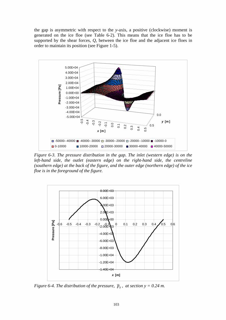
103

the gap is asymmetric with respect to the y-axis, a positive (clockwise) moment is generated on the ice floe (see Table 6-2). This means that the ice floe has to be supported by the shear forces, Q, between the ice floe and the adjacent ice floes in order to maintain its position (see Figure 1-5).

-0.5

-0.4

-0.3

-0.2

-0.1

0.0

0.1

0.2

0.3

0.4

0.5

0.5

0.0-5.00E+04-4.00E+04-3.00E+04-2.00E+04-1.00E+040.00E+001.00E+042.00E+043.00E+044.00E+045.00E+04

Pres

sure

[Pa]

x [m ]

y [m ]

-50000--40000 -40000--30000 -30000--20000 -20000--10000 -10000-0

0-10000 10000-20000 20000-30000 30000-40000 40000-50000

Figure 6-3. The pressure distribution in the gap. The inlet (western edge) is on the left-hand side, the outlet (eastern edge) on the right-hand side, the centreline (southern edge) at the back of the figure, and the outer edge (northern edge) of the ice floe is in the foreground of the figure.

-1.40E+04

-1.20E+04

-1.00E+04

-8.00E+03

-6.00E+03

-4.00E+03

-2.00E+03

0.00E+00

2.00E+03

4.00E+03

6.00E+03

8.00E+03

-0.6 -0.5 -0.4 -0.3 -0.2 -0.1 0 0.1 0.2 0.3 0.4 0.5 0.6

x [m]

Pres

sure

[Pa]

Figure 6-4. The distribution of the pressure, dp , at section y = 0.24 m.

104

There is no cavitation in the gap, since the minimum dynamic pressure in the gap, about –50 kPa, plus the atmospheric pressure, about 100 kPa, is much higher than the vapour pressure of water, 0.61 kPa, even if the hydrostatic pressure were small; see Equation (5.50). Analysis of the flow in the gap using Equation (5.58) indicated that flow film separation does not occur in the gap. In Figure 6-3 it can also be seen that the pressure at the northern edge is not zero.

0

0.5

1

1.5

2

2.5

3

3.5

-0.6 -0.5 -0.4 -0.3 -0.2 -0.1 0 0.1 0.2 0.3 0.4 0.5 0.6

x [m]

u m [m

/s]

Figure 6-5. The mean velocity, um, in the x-coordinate direction in the gap at y = 0.24 m.

-1

-0.5

0

0.5

1

1.5

-0.6 -0.5 -0.4 -0.3 -0.2 -0.1 0 0.1 0.2 0.3 0.4 0.5 0.6

x [m]

v m [m

/s]

Figure 6-6. The mean velocity, vm, in the y-coordinate direction in the gap at y = 0.24 m.

105

The distribution of the velocity in the x-coordinate direction and in the y-coordinate direction and the shear stress distribution on the lower wall at y = 0.24 m are depicted in Figures 6-5 to 6-7, respectively. The convergence of the iteration is depicted in Figure 6-8. In this figure it can be seen that the value of 0.5⋅10-8 of the L2 norm of the change of velocity in the x-coordinate direction is an appropriate criterion for the convergence of the outer iteration.

-20

-10

0

10

20

30

40

50

60

70

-0.6 -0.5 -0.4 -0.3 -0.2 -0.1 0 0.1 0.2 0.3 0.4 0.5 0.6

x [m]

Shea

r str

ess

at th

e lo

wer

wal

l [N

/mm

2 ]

Figure 6-7. The shear stress distribution on the lower wall in section y = 0.24 m.

1E-11

1E-10

1E-09

1E-08

1E-07

1E-06

1E-05

0.0001

0.001

0.01

0.1

1

10

100

1000

0 500 1000 1500 2000 2500

Number of iteration cycles

L2 o

f dm

, du

m, d

vm

or d

pd

L2_of_dpL2_of_duL2_of_dvL2_of_dm

Figure 6-8. The convergence of the iteration showing the L2 norms for the mass balance, for the velocities in the x- and y-coordinate directions, and for the pressure in the cells of the calculation domain.

106

In order to confirm the periodicity of the flow, two ice floes of equal size were set one after another, and the calculations were performed with the same parameters as given in Table 6-1. The velocity distribution in the section y = 0.25 m along the floes is presented in Figure 6-9. The same kind of periodicity could also be found for the other flow variables.

0

0.5

1

1.5

2

2.5

3

3.5

-1 -0.5 0 0.5 1 1.5 2

x [m]

u m [m

/s]

Figure 6-9. The mean velocity in the x-coordinate direction, um, in the gap at y = 0.25 m for two adjacent floes. 6.1.1.2 Case 2: Leakage occurs through the gap between the ice floes at the

northern edge The previous calculations were performed by using periodic boundary conditions between the western (inlet) and the eastern (outlet) boundaries of the calculation domain, and the symmetric boundary condition on the southern and northern edges. The flow in this case is like a "channel flow" in the gap between the ice floe, the hull surface, and the southern and northern edges, with no leakage in or out of the calculation domain through the small gaps between the adjacent ice floes. The calculations were now repeated using the inflow boundary condition at the western edge and the outflow boundary condition at the eastern edge (see Section 5.3.4.4) and the free flow boundary condition at the northern edge of the calculation domain (see Section 5.3.4.5). The pressure was set to zero at the western, northern, and eastern edges of the calculation domain. As in Case 1, the symmetry boundary condition was set at the southern edge. The results of the calculations are shown in Table 6-3. The pressure field is depicted in Figure 6-10. The average pressure in the gap is higher than in Case 1, but is still negative. Table 6-3. Results of the calculations for Case 2.

Mass flow through edges [kg/s] Western

edge (inlet)

Northern edge

Eastern edge

(outlet)

Average pressure in the gap,

1

*dp [Pa]

Moment about the y-

axis [Nm]

Average shear stress on the

ice floe [N/m2]

1.396 0.634 -2.030 -733.94 1012.48 24.823

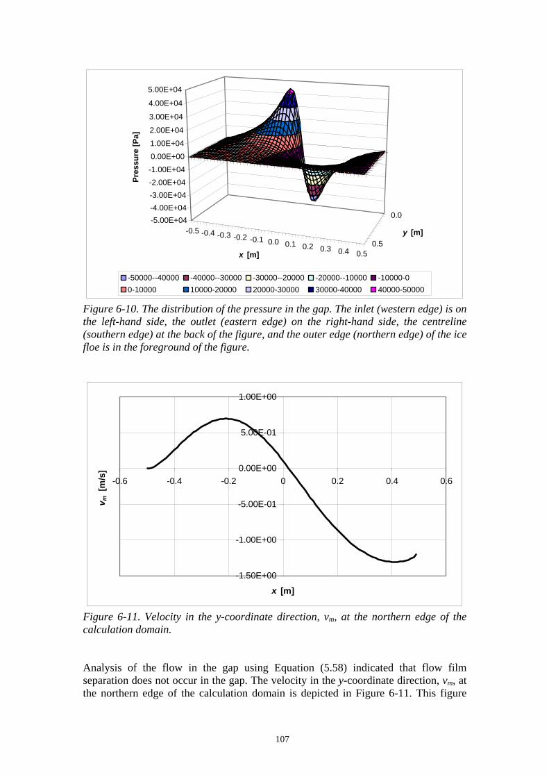
107

-0.5 -0.4 -0.3 -0.2 -0.1 0.0 0.1 0.2 0.3 0.4 0.50.5

0.0-5.00E+04-4.00E+04-3.00E+04-2.00E+04-1.00E+040.00E+00

1.00E+04

2.00E+04

3.00E+04

4.00E+04

5.00E+04

Pres

sure

[Pa]

x [m]

y [m]

-50000--40000 -40000--30000 -30000--20000 -20000--10000 -10000-00-10000 10000-20000 20000-30000 30000-40000 40000-50000

Figure 6-10. The distribution of the pressure in the gap. The inlet (western edge) is on the left-hand side, the outlet (eastern edge) on the right-hand side, the centreline (southern edge) at the back of the figure, and the outer edge (northern edge) of the ice floe is in the foreground of the figure.

-1.50E+00

-1.00E+00

-5.00E-01

0.00E+00

5.00E-01

1.00E+00

-0.6 -0.4 -0.2 0 0.2 0.4 0.6

x [m]

v m [

m/s

]

Figure 6-11. Velocity in the y-coordinate direction, vm, at the northern edge of the calculation domain. Analysis of the flow in the gap using Equation (5.58) indicated that flow film separation does not occur in the gap. The velocity in the y-coordinate direction, vm, at the northern edge of the calculation domain is depicted in Figure 6-11. This figure

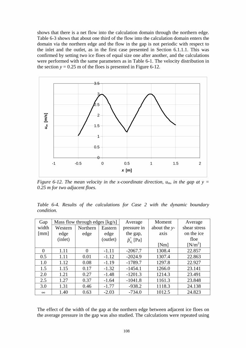
108

shows that there is a net flow into the calculation domain through the northern edge. Table 6-3 shows that about one third of the flow into the calculation domain enters the domain via the northern edge and the flow in the gap is not periodic with respect to the inlet and the outlet, as in the first case presented in Section 6.1.1.1. This was confirmed by setting two ice floes of equal size one after another, and the calculations were performed with the same parameters as in Table 6-1. The velocity distribution in the section y = 0.25 m of the floes is presented in Figure 6-12.

0

0.5

1

1.5

2

2.5

3

3.5

-1 -0.5 0 0.5 1 1.5 2

x [m]

u m [m

/s]

Figure 6-12. The mean velocity in the x-coordinate direction, um, in the gap at y = 0.25 m for two adjacent floes. Table 6-4. Results of the calculations for Case 2 with the dynamic boundary condition.

Mass flow through edges [kg/s]Gap width [mm]

Western edge

(inlet)

Northern edge

Eastern edge

(outlet)

Average pressure in

the gap,

1

*dp [Pa]

Moment about the y-

axis

[Nm]

Average shear stress on the ice

floe [N/m2]

0 1.11 0 -1.11 -2067.7 1308.4 22.857 0.5 1.11 0.01 -1.12 -2024.9 1307.4 22.863 1.0 1.12 0.08 -1.19 -1789.7 1297.8 22.927 1.5 1.15 0.17 -1.32 -1454.1 1266.0 23.141 2.0 1.21 0.27 -1.48 -1201.3 1214.3 23.491 2.5 1.27 0.37 -1.64 -1041.8 1161.3 23.848 3.0 1.31 0.46 -1.77 -938.2 1118.3 24.138 ∞ 1.40 0.63 -2.03 -734.0 1012.5 24.823

The effect of the width of the gap at the northern edge between adjacent ice floes on the average pressure in the gap was also studied. The calculations were repeated using

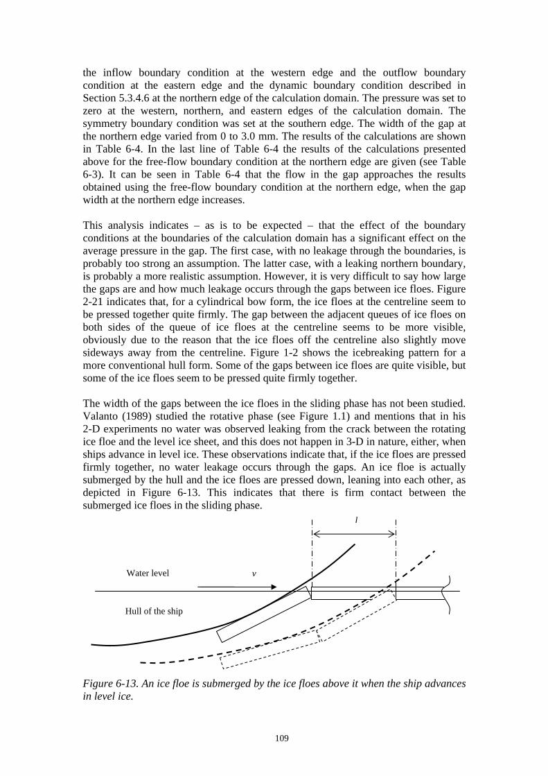
109

the inflow boundary condition at the western edge and the outflow boundary condition at the eastern edge and the dynamic boundary condition described in Section 5.3.4.6 at the northern edge of the calculation domain. The pressure was set to zero at the western, northern, and eastern edges of the calculation domain. The symmetry boundary condition was set at the southern edge. The width of the gap at the northern edge varied from 0 to 3.0 mm. The results of the calculations are shown in Table 6-4. In the last line of Table 6-4 the results of the calculations presented above for the free-flow boundary condition at the northern edge are given (see Table 6-3). It can be seen in Table 6-4 that the flow in the gap approaches the results obtained using the free-flow boundary condition at the northern edge, when the gap width at the northern edge increases. This analysis indicates – as is to be expected – that the effect of the boundary conditions at the boundaries of the calculation domain has a significant effect on the average pressure in the gap. The first case, with no leakage through the boundaries, is probably too strong an assumption. The latter case, with a leaking northern boundary, is probably a more realistic assumption. However, it is very difficult to say how large the gaps are and how much leakage occurs through the gaps between ice floes. Figure 2-21 indicates that, for a cylindrical bow form, the ice floes at the centreline seem to be pressed together quite firmly. The gap between the adjacent queues of ice floes on both sides of the queue of ice floes at the centreline seems to be more visible, obviously due to the reason that the ice floes off the centreline also slightly move sideways away from the centreline. Figure 1-2 shows the icebreaking pattern for a more conventional hull form. Some of the gaps between ice floes are quite visible, but some of the ice floes seem to be pressed quite firmly together. The width of the gaps between the ice floes in the sliding phase has not been studied. Valanto (1989) studied the rotative phase (see Figure 1.1) and mentions that in his 2-D experiments no water was observed leaking from the crack between the rotating ice floe and the level ice sheet, and this does not happen in 3-D in nature, either, when ships advance in level ice. These observations indicate that, if the ice floes are pressed firmly together, no water leakage occurs through the gaps. An ice floe is actually submerged by the hull and the ice floes are pressed down, leaning into each other, as depicted in Figure 6-13. This indicates that there is firm contact between the submerged ice floes in the sliding phase. Figure 6-13. An ice floe is submerged by the ice floes above it when the ship advances in level ice.

v

l

Hull of the ship

Water level

110

6.1.2 The effect of pressure below the ice floes on ice resistance due to the sliding phase

Changes in pressure below the ice floes was discussed in Section 1.6. All the previous calculations were performed assuming that the pressure is zero at all boundaries of the ice floe. The calculations were now repeated assuming that even if the ice floes are in contact with each other, the pressure below the ice floe, denoted as

2dp in Section 1.5, has an effect on the pressure in the gap between the hull surface and the ice floe through the gaps between the ice floe and the ice floes adjacent to it. It was further assumed that the pressure around the calculation domain changes linearly from zero at the western edge to a certain value at the eastern edge of the calculation domain. In other words, there is a pressure gradient between the western and eastern edges. Calculations were performed for three cases using the following values of pressure at the eastern edge: -500 Pa, 0 Pa and 500 Pa. The inflow boundary condition was used at the western edge and the outflow boundary condition at the eastern edge (see Section 5.3.4.4) and the free flow boundary condition at the northern edge of the calculation domain (see Section 5.3.4.5). At the southern edge, the symmetry boundary condition was set. The parameters given in Table 6-1 were used in the calculations except that it was assumed that the velocity of the hull surface was 1 m/s and thus the flow in the gap between the hull surface and the ice floe was laminar. The results of the calculations are shown in Table 6-5 and the pressure distribution in the gap at y = 0.25 m is depicted in Figure 6-14. Table 6-5. The results of the calculations.

Mass flow through edges [kg/s] Pressure at the

eastern edge [Pa]

Western edge

(inlet)

Northern edge

Eastern edge

(outlet)

Average change in pressure in

the gap,

1dp [Pa]

Moment about the y-

axis [Nm]

Average shear

stress on the ice

floe [N/m2]

-500 0.334460 0.092996 -0.42746 -259.801 167.759 2.06 0 0.282989 0.061850 -0.34484 -1.345 116.139 1.82 500 0.215420 0.039880 -0.25530 256.851 64.677 1.58

The results indicate that negative pressure at the northern and eastern edges increase the flow in the gap, which results in decrease of the pressure in the gap. In a similar way, overpressure at these edges decreases the flow in the gap and consequently increases the pressure in the gap. However, the “net effect” of the pressure below the ice floe on level ice resistance is almost zero, because the effect of the average dynamic pressure below the ice floe,

2dp = ∓ 250 Pa, on ice resistance is almost cancelled by the change of the pressure in the gap between the hull surface and the ice floe. This conclusion is not exactly correct in cases when the dynamic pressure below the ice floe does not change linearly between the edges of the ice floe, because the gap between the hull surface and the ice floe “feels” the pressure below the ice floe only through the gaps between the ice floe and the ice floes adjacent to it.

111

This analysis does not take into account the fact that the dynamic pressure below the ice floe changes with time as the hull glides over it, see Figure 1-6. Naturally, the tightness of the gaps between the adjacent ice floes should also be taken into account, if the effect of the pressure below the ice floes is properly taken into account in the analysis. This is clearly an area which needs further research.

-1200-1000

-800-600-400-200

0200400600800

1000

-0.5 0 0.5

x [m]

Pres

sure

[Pa] p = 500 Pa at the eastern

edgep = 0 at the eastern edge

p = -500 Pa at theeastern edge

Figure 6-14. The distribution of the pressure in the gap between the hull surface and the ice floe at y = 0.25 m. The inlet (western edge) is on the left-hand side and the outlet (eastern edge) on the right-hand side. 6.1.3 Variation of the computational parameters and the effect of the

turbulence model on the results The under-relaxation parameters for the calculation of the average velocity and the pressure in the gap were varied in order to gain an idea of their effect on the speed of the convergence of the iteration. The grid size was also varied in order to find its effect on the solution. The calculations were performed using two turbulence models, the turbulence model of Constantinescu and the turbulence model of Hirs. In the following paragraphs the results of the calculations are shown for Case 1, the "channel flow", in the gap. 6.1.3.1 Variation of the under-relaxation parameters The effect of the under-relaxation parameter for the calculation of the pressure is demonstrated in Figure 6-15. The calculations were performed with the same parameters as given in Section 6.1.1 for Case 1. In Figure 6-15 the effect of Patankar's under-relaxation (see Section 5.3.2) can be clearly seen: the number of inner iterations decreases dramatically, from almost 800 iteration cycles to 3 cycles, when the value of the under-relaxation parameter for pressure, pα (see Section 5.3.2), decreases from 1.0 to 0.05. The optimal value for the under-relaxation parameter for pressure for the selected calculation parameters seems

112

to be about 0.5, when the product of the number of the inner and outer iterations has a minimum value of about 6000.

1.00E+00

1.00E+01

1.00E+02

1.00E+03

1.00E+04

1.00E+05

1.00E+06

0 0.2 0.4 0.6 0.8 1 1.2

Under-relaxation factor for pressure

ITER

,ITLG

SM,IT

ER*IT

LGSM

ITERITLGSMITER*ITLGSM

Figure 6-15. The effect of the variation of the under-relaxation parameter for pressure, pα , on the number of iterations. ITER means the number of outer iterations and ITLGSM means the number of inner iterations.

0

500

1000

1500

2000

2500

0 0.05 0.1 0.15 0.2 0.25 0.3 0.35

Under-relaxation parameter for velocity

ITER

Figure 6-16. The effect of the under-relaxation parameter for velocity, α , on the number of outer iterations.

113

The effect of the under-relaxation parameter for velocity, α (see Section 5.3.3), on the number of outer iterations is shown in Figure 6-16. The under-relaxation parameter for pressure was 0.2 and the other parameters are the same as in Section 6.1.1. An oscillating solution was obtained when the value of the under-relaxation parameter for velocity was higher than or equal to 0.35. The optimal parameters for the under-relaxation factors for the problem given in Section 6.1.1 are thus 0.5 for pressure and 0.3 for velocity. 6.1.3.2 The effect of the grid density on the solution The effect of the grid density on the solution was studied by varying the number of cells in the x- and y-coordinate directions. The effect of the grid density on the average pressure in the gap is shown in Figure 6-17. The accuracy of the solution naturally increases when the grid size is refined, because a fine grid can take into account the geometry of the gap better than a coarse grid. Additionally, the derivatives can be calculated more accurately on a fine grid. Richardson's extrapolation (see Ferziger and Peric (2002), pp. 58-60) was applied in order to estimate the accurate value of the mass flow at the inlet, the shear stress on the lower wall, and the average pressure in the gap. The results are presented in Tables 6-6 and 6-7 using the turbulence models of Constantinescu and Hirs, respectively. Table 6-6. Estimate of the exact values of mass flow, average shear stress, and average pressure in the gap according to Richardson's extrapolation (turbulence model of Constantinescu).

imax jmax Mass flow [kg/s]

Average shear stress

[N/m2]

Average pressure,

1

*dp [Pa]

Error for calculation of pressure [%]

40 20 1.09447 21.82 -1962.7 2.64 80 40 1.09603 21.85 -1983.4 1.61 160 80 1.09627 21.87 -1996.1 0.99

"Exact" by extrapolation 1.09631 21.95 -2016.0 Table 6-7. Estimate of the exact values of mass flow, average shear stress, and average pressure in the gap according to Richardson's extrapolation (turbulence model of Hirs).

imax jmax Mass flow [kg/s]

Average shear stress

[N/m2]

Average pressure,

1

*dp [Pa]

Error for calculation of pressure [%]

40 20 1.10831 22.87 -2007.2 3.65 80 40 1.10999 22.91 -2039.7 2.09 160 80 1.11029 22.94 -2058.4 1.20

"Exact" by extrapolation 1.11035 23.01 -2083.3

114

-2050

-2000

-1950

-1900

-1850

-1800

-17500 2000 4000 6000 8000 10000 12000 14000

Grid size (i max*j max)

Ave

rage

pre

ssur

e in

the

gap

[Pa]

Figure 6-17. The effect of the grid density on the average pressure in the gap. The turbulence model of Constantinescu was used in the calculations. 6.1.3.3 The effect of the turbulence model on the results of the calculations Three turbulence models were presented in Section 5.2.4: the turbulence model of Constantinescu (see Constantinescu and Geletuse (1974)); the turbulence model of Hirs (see Hirs (1973)), and the turbulence model of Ng and Pan (see Ng and Pan (1965). Since the turbulence model of Constantinescu seems to be almost identical to the turbulence model of Ng and Pan, the calculations were performed using the turbulence models of Constantinescu and Hirs. The results are given in Tables 6-6 and 6-7. The results of the calculations do not seem to differ very significantly from each other. 6.1.4 Variation of the geometric parameters The geometric parameters were varied in order to gain an idea of their effect on the results of the calculations, particularly on the average pressure in the gap. The basic parameters were the same as in Section 6.1.1. The following parameters were varied: the minimum distance between the hull surface and the ice floe, hmin, the radii of the hull surface, Rx and Ry, the velocity of the upper wall, U, the position of the ice floe, and the area of the ice floe. In the following paragraphs the results of the calculations are presented for Case 1, the "channel flow" in the gap. 6.1.4.1 Contact between the hull surface and the ice floe The previous calculations were performed on the basis of the assumption that the hull surface and the ice floe are separated from each other by a small distance, hmin = 0.1 mm. It is now assumed that there is an elastic contact between the surfaces; see Figure 6-18.

115

Figure 6-18. Elastic contact between two surfaces. The radius of the contact area, a, between two balls in elastic contact is, according to Kivioja et al. (2001):

'

3'

34

nF RaE

= , (6.1)

where Fn is the normal force between the balls and R' is the combined radius of the surfaces:

'1 2

1 1 1R R R

= + , (6.2)

where R1 and R2 are the radii of the surfaces and E' is the combined modulus of elasticity for the materials of the balls:

2 21 2

'1 2

1 1 1E E E

ν ν− −= + , (6.3)

where E1 and E2 are the moduli of elasticity and 1ν and 2ν are the Poisson coefficients of the balls. Assuming that the hull is a "steel ball", R1 = 75 m, E1 = 206 GPa, and

1 0.3ν = , and the ice floe is an "ice ball", R2 = ∞ m, E2 = 4 GPa, and 2ν = 0.3, and Fn ≈ 2500 N (2000 N as a result of dynamic pressure and 490 N as a result of the static lift of an ice floe with a thickness of 0.5 m), the radius of the contact area is 0.0319 m. The area of the circular contact area is thus about 0.0032 m2. The calculation of the flow in the gap was next carried out on the basis of the assumption that there is a contact area of 0.0032 m2 between the surfaces. The cells in the calculation domain which are in the contact area were considered as obstacle cells where no fluid flow exists. The no-slip boundary conditions described in Section 5.3.4.1 were set at the boundaries of the obstacle cells and the calculation domain. The result of the calculation gives an average pressure in the gap between the hull surface and the ice floe of -2024 N. Comparing this figure with the data given in Table 6-7, it can be concluded that the elastic contact between the two surfaces has a negligible effect on the average pressure in the gap compared with the results obtained when the distance between the two surfaces is e.g. 0.1 mm. It is more convenient to

a

2a

Half of the contact area

116

perform the calculations for the case with a small minimum distance between the surfaces than for the case with elastic contact, since the convergence of the former calculation is two orders of magnitude faster than for the latter. For this reason the calculations in the following paragraphs were performed with a small minimum distance of 0.1 mm assumed between the surfaces. 6.1.4.2 Minimum distance between the surfaces The effect of the minimum distance between the hull and ice surfaces on the average pressure in the gap can be seen in Figure 6-19. The calculations and the analysis presented in the previous section show that the average pressure seems to be almost constant when 0.0 mm minh≤ ≤ 0.1 mm.

-2500

-2000

-1500

-1000

-500

01.00E-05 1.00E-04 1.00E-03 1.00E-02

Distance of the walls [m]

Ave

rage

pre

ssur

e [P

a]

Figure 6-19. Average pressure in the gap when the minimum distance between the hull and ice surfaces varies from 0.01 mm to 10 mm. The effect of the minimum distance between the surfaces on the average shear stress on the ice surface is shown in Figure 6-20. The distance between the surfaces was varied from 0.0 mm to 0.5 mm. The calculations indicate that the average shear stress on the lower surface increases to a certain level with decreasing minimum distance and then slightly decreases when there is contact between the surfaces. The reason for this is that high shear stresses occur at the area of the minimum distance between the surfaces when the surfaces are slightly separated. When the surfaces are in contact, it was assumed that no fluid flow took place in the contact area.

117

0

5

10

15

20

25

30

0 0.1 0.2 0.3 0.4 0.5

Distance of the walls [mm]

Ave

rage

she

ar s

tres

s on

the

low

er w

all

[N/m

2 ]

Figure 6-20. Average shear stress on the lower surface when the minimum distance between the hull and the ice surfaces varies from 0.0 mm to 0.5 mm. 6.1.4.3 Variation of the size of the ice floe The effect of the size of the ice floe on the average pressure between the hull and the ice floe was studied by varying the breadth of the ice floe, the length of the ice floe, and the area of the ice floe. The other parameters were the same as in Section 6.1.1.

-2500

-2000

-1500

-1000

-500

00 0.5 1 1.5 2 2.5 3 3.5

b [m] or l [m]

Ave

rage

pre

ssur

e in

the

gap

[Pa]

Variation of the breadthof the ice floeVariation of the length ofthe ice floe

Figure 6-21. The effect of the variation of the breadth, b, and the length, l, of the ice floe on the average pressure in the gap.

118

The results for the variation of the breadth and the length of the ice floe are shown in Figure 6-21, where it can be observed that the average pressure in the gap reaches its minimum when the ice floe is square-shaped. The results for the variation of the area of the square-shaped ice floe are shown in Figures 6-22 and 6-23. The average pressure in the gap decreases with increasing flow area, as can be seen in Figure 6-22. The average shear stress on the ice surface increases with decreasing floe size, as can be seen in Figure 6-23. This is logical, because the average distance between the hull surface and the ice floes also decreases with decreasing floe size.

-2500

-2000

-1500

-1000

-500

00 0.5 1 1.5 2 2.5

Area of the ice floe [m2]

Ave

rage

pre

ssur

e in

the

gap

[Pa]

Figure 6-22. The effect of the variation of the area of the square-shaped ice floe on the average pressure in the gap.

0

10

20

30

40

50

60

70

80

90

0 0.5 1 1.5 2 2.5

Area of the ice floe [m2]

Ave

rage

she

ar s

tres

s on

the

low

er w

all

[N/m

2 ]

Figure 6-23. The effect of the variation of the area of the ice floe on the average shear stress on the surface of the ice floe.

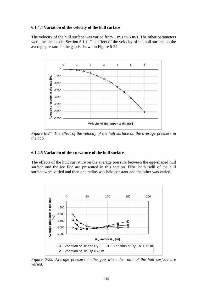
119

6.1.4.4 Variation of the velocity of the hull surface The velocity of the hull surface was varied from 1 m/s to 6 m/s. The other parameters were the same as in Section 6.1.1. The effect of the velocity of the hull surface on the average pressure in the gap is shown in Figure 6-24.

-3500

-3000

-2500

-2000

-1500

-1000

-500

00 1 2 3 4 5 6 7

Velocity of the upper w all [m /s]

Ave

rage

pre

ssur

e in

the

gap

[Pa]

Figure 6-24. The effect of the velocity of the hull surface on the average pressure in the gap. 6.1.4.5 Variation of the curvature of the hull surface The effects of the hull curvature on the average pressure between the egg-shaped hull surface and the ice floe are presented in this section. First, both radii of the hull surface were varied and then one radius was held constant and the other was varied.

-2500

-2000

-1500

-1000

-500

00 50 100 150 200

R x and/or R y [m]

Ave

rage

pre

ssur

e in

the

gap

[Pa]

Variation of Rx and Ry Variation of Ry, Rx = 75 mVariation of Rx, Ry = 75 m

Figure 6-25. Average pressure in the gap when the radii of the hull surface are varied.

120

First, both radii of the hull surface, Rx and Ry, were varied from 15 m to 150 m. The effect of the radii of the hull surface on the average pressure in the gap is depicted in Figure 6-25. The average pressure seems to be at a minimum when both Rx and Ry are about 35 m. When the curvature of the hull surface approaches infinity, the average pressure in the gap approaches zero, as the flow approaches the Couette flow between two parallel walls. The radius of the hull surface in the y-coordinate direction, Ry, was varied while the radius of the hull surface in the x-coordinate direction was kept constant, Rx = 75 m. The average pressure is now at its minimum when Ry = 50 m. Finally, the radius of the hull surface in the x-coordinate direction, Rx, was varied while the radius of the hull surface in the y-coordinate direction was kept constant, Ry = 75 m. The average pressure in the gap is now at its minimum when Rx = 100 m (see Figure 6-25). 6.1.4.6 The effect of the inclination of the ice floe on the pressure in the gap All the previous calculations were performed for a symmetric geometry of the gap; see Case 1 in Figure 6-26. The case where the gap is not symmetrical but inclined with respect to the y-coordinate axis is now considered. This is achieved by shifting the contact point of the ice floe with the hull surface forwards or backwards along the x-coordinate axis. The gap is thus still symmetrical with respect to the x-coordinate axis. Two cases where the flow is assumed to be periodic, as depicted in Figure 6-26, are now considered. In Case 2 the gap at the western edge (inlet) is larger than the gap at the eastern edge (outlet). In Case 3 the gap at the inlet is smaller than the gap at the outlet. The other parameters were the same as in Table 6-1. The results of the analysis are shown in Figure 6-27. In Figure 6-27 the significant effect of the position of the ice floe on the average pressure in the gap can be observed. If the inclination angle is -0.23 degrees (the contact point of the ice floe is moved 0.15 m in the negative x-coordinate direction), a considerable decrease in pressure can be seen to exist in the gap, whereas if the inclination angle is 0.23 degrees (the contact point of the ice floe is moved 0.15 m in the positive x-coordinate direction), a considerable increase in pressure exists in the gap. The turning moment on the ice floe resulting from the pressure in the gap is always positive. This means that the pressure distribution in the gap seems to favour Case 2. In ice model tests in thick ice the layer of broken ice floes is quite stable and the floes keep together as is shown in Figure 1-2. However, at high speed in thin level ice the broken ice floes do not stay together under the hull but stray further away from the hull quite early, and result in “a cloud” of ice floes around the hull of the ship. This phenomenon may be at least partly explained by the positive moment due to asymmetric pressure distribution in the gap between the hull and the ice floes.

121

Figure 6-26. The considered cases with an inclined ice floe.

-6000

-5000

-4000

-3000

-2000

-1000

0

1000

2000

3000

-0.2 -0.15 -0.1 -0.05 0 0.05 0.1 0.15 0.2

d xl [m]

Ave

rage

pre

ssur

e [P

a] o

r tur

ning

m

omen

t [N

m]

Average pressureTurning moment

Figure 6-27. Average pressure in the gap,

1

*dp , and the turning moment about the

y-coordinate axis for the inclined ice floe resulting from the pressure in the gap. The distance of the contact point of the ice floe and the hull surface measured from the centre of the ice floe is dxl.

v

Case 2

v

Case 3

v

Case 1

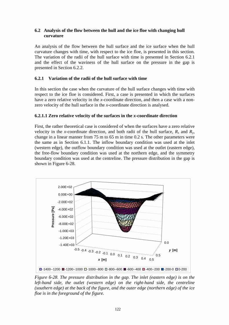
122

6.2 Analysis of the flow between the hull and the ice floe with changing hull curvature

An analysis of the flow between the hull surface and the ice surface when the hull curvature changes with time, with respect to the ice floe, is presented in this section. The variation of the radii of the hull surface with time is presented in Section 6.2.1 and the effect of the waviness of the hull surface on the pressure in the gap is presented in Section 6.2.2. 6.2.1 Variation of the radii of the hull surface with time In this section the case when the curvature of the hull surface changes with time with respect to the ice floe is considered. First, a case is presented in which the surfaces have a zero relative velocity in the x-coordinate direction, and then a case with a non-zero velocity of the hull surface in the x-coordinate direction is analysed. 6.2.1.1 Zero relative velocity of the surfaces in the x-coordinate direction First, the rather theoretical case is considered of when the surfaces have a zero relative velocity in the x-coordinate direction, and both radii of the hull surface, Rx and Ry, change in a linear manner from 75 m to 65 m in time 0.2 s. The other parameters were the same as in Section 6.1.1. The inflow boundary condition was used at the inlet (western edge), the outflow boundary condition was used at the outlet (eastern edge), the free-flow boundary condition was used at the northern edge, and the symmetry boundary condition was used at the centreline. The pressure distribution in the gap is shown in Figure 6-28.

-0.5 -0.4 -0.3 -0.2 -0.1 0.0 0.1 0.2 0.3 0.4 0.50.5

0.0-1.40E+03

-1.20E+03

-1.00E+03

-8.00E+02

-6.00E+02

-4.00E+02

-2.00E+02

0.00E+00

2.00E+02

Pres

sure

[Pa]

x [m]

y [m]

-1400--1200 -1200--1000 -1000--800 -800--600 -600--400 -400--200 -200-0 0-200

Figure 6-28. The pressure distribution in the gap. The inlet (eastern edge) is on the left-hand side, the outlet (western edge) on the right-hand side, the centreline (southern edge) at the back of the figure, and the outer edge (northern edge) of the ice floe is in the foreground of the figure.

123

It can be seen in Figure 6-28 that negative pressure resulting from the separation of the surfaces occurs in the gap. The pressure has the lowest value at the point where the distance between the surfaces has the smallest value. This observation is in line with Equation (5.131), which indicates that the pressure in the gap is inversely proportional to the third power of the distance between the surfaces. 6.2.1.2 Non-zero relative velocity of the surfaces in the x-coordinate direction In this section the case is considered of when the radii of the hull surface, Rx and Ry, change linearly from 75 m to 65 m within a distance of 1 m in the x–coordinate direction and the hull surface has a non-zero velocity in the x-coordinate direction. The speed of the ship was varied from 1 m/s to 5 m/s. The time during which the hull geometry changes, t, depends on the speed of the ship (see Table 6-8). The other parameters were the same as in Section 6.1.1. The results of the calculations are shown in Figure 6-29. Table 6-8. The time during which the radius of the hull surface changes from 75 m to 65 m.

v [m/s] t [s] 1 1.00 2 0.50 3 0.33 4 0.25 5 0.20

-3500

-3000

-2500

-2000

-1500

-1000

-500

00 1 2 3 4 5 6

Velocity of the hull surface [m/s]

Ave

rage

pre

ssur

e in

the

gap

[Pa]

Constant hull curvatureIncreasing hull curvature

Figure 6-29. The average pressure in the gap resulting from constant and increasing hull curvature.

124

In Figure 6-29 it can be observed that the average pressure in the gap decreases considerably as a result of increasing hull curvature. The pressure in the gap is lower the faster the ship moves. 6.2.2 The effect of the waviness of the hull surface In reality the plating of the hull surface may have permanent deformations caused by ice loads or slamming pressure loads. It is assumed that the “waviness” of the hull can be expressed as follows:

max cos sinx y

h h x yπ πλ λ

⎛ ⎞⎛ ⎞Δ = Δ ⎜ ⎟⎜ ⎟ ⎜ ⎟⎝ ⎠ ⎝ ⎠

, (6.4)

where hΔ is the permanent deflection of the hull plating, maxhΔ is the maximum permanent deflection, xλ is the wavelength of the permanent deflection in the x–coordinate direction and yλ is the wavelength of the permanent deflection in the y–coordinate direction. The waviness of the hull surface calculated using Equation (6.4) is depicted in Figure 6-30 using the following parameters: maxhΔ = 0.0001 m,

xλ = 1.0 m and yλ = 1.0 m.

-0.5 -0.4 -0.3 -0.2 -0.1 0.0 0.1 0.2 0.3 0.4 0.50.5

0.00.00E+00

1.00E-05

2.00E-05

3.00E-05

4.00E-05

5.00E-05

6.00E-05

7.00E-05

8.00E-05

9.00E-05

1.00E-04

dh [m ]

x [m ]

y [m ]

Figure 6-30. Waviness of the hull surface compared with the un-deformed hull surface. The flow in the gap between the wavy hull surface and an ice floe was calculated using the parameters given in Section 6.1.1. The flow is now time-dependent as a result of the waviness of the hull surface. The average pressure in the gap is shown in Figure 6-31. The average pressure seems to fluctuate quite considerably, even if the

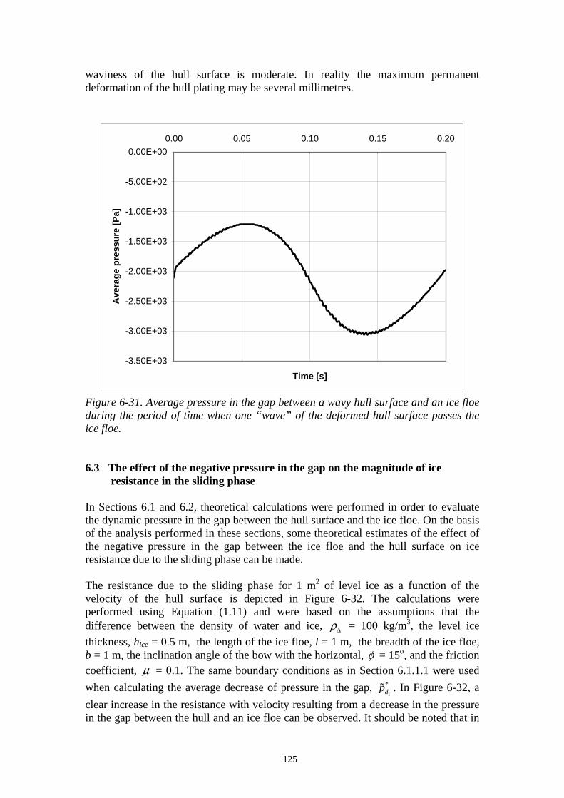
125

waviness of the hull surface is moderate. In reality the maximum permanent deformation of the hull plating may be several millimetres.

-3.50E+03

-3.00E+03

-2.50E+03

-2.00E+03

-1.50E+03

-1.00E+03

-5.00E+02

0.00E+000.00 0.05 0.10 0.15 0.20

Time [s]

Ave

rage

pre

ssur

e [P

a]

Figure 6-31. Average pressure in the gap between a wavy hull surface and an ice floe during the period of time when one “wave” of the deformed hull surface passes the ice floe. 6.3 The effect of the negative pressure in the gap on the magnitude of ice resistance in the sliding phase In Sections 6.1 and 6.2, theoretical calculations were performed in order to evaluate the dynamic pressure in the gap between the hull surface and the ice floe. On the basis of the analysis performed in these sections, some theoretical estimates of the effect of the negative pressure in the gap between the ice floe and the hull surface on ice resistance due to the sliding phase can be made. The resistance due to the sliding phase for 1 m2 of level ice as a function of the velocity of the hull surface is depicted in Figure 6-32. The calculations were performed using Equation (1.11) and were based on the assumptions that the difference between the density of water and ice, ρΔ = 100 kg/m3, the level ice thickness, hice = 0.5 m, the length of the ice floe, l = 1 m, the breadth of the ice floe, b = 1 m, the inclination angle of the bow with the horizontal, φ = 15o, and the friction coefficient, μ = 0.1. The same boundary conditions as in Section 6.1.1.1 were used when calculating the average decrease of pressure in the gap,

1

*dp . In Figure 6-32, a

clear increase in the resistance with velocity resulting from a decrease in the pressure in the gap between the hull and an ice floe can be observed. It should be noted that in

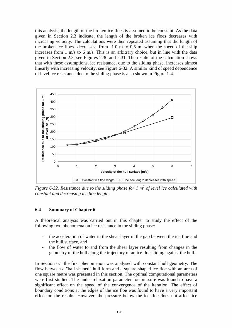
126

this analysis, the length of the broken ice floes is assumed to be constant. As the data given in Section 2.3 indicate, the length of the broken ice floes decreases with increasing velocity. The calculations were then repeated assuming that the length of the broken ice floes decreases from 1.0 m to 0.5 m, when the speed of the ship increases from 1 m/s to 6 m/s. This is an arbitrary choice, but in line with the data given in Section 2.3, see Figures 2.30 and 2.31. The results of the calculation shows that with these assumptions, ice resistance, due to the sliding phase, increases almost linearly with increasing velocity, see Figure 6-32. A similar kind of speed dependence of level ice resistance due to the sliding phase is also shown in Figure 1-4.

0

50

100

150

200

250

300

350

400

450

0 1 2 3 4 5 6 7

Velocity of the hull surface [m/s]

Res

ista

nce

due

to th

e sl

indi

ng p

hase

for 1

m2

of le

vel i

ce [

N]

Constant ice floe length Ice floe length decreases with speed

Figure 6-32. Resistance due to the sliding phase for 1 m2 of level ice calculated with constant and decreasing ice floe length. 6.4 Summary of Chapter 6 A theoretical analysis was carried out in this chapter to study the effect of the following two phenomena on ice resistance in the sliding phase:

- the acceleration of water in the shear layer in the gap between the ice floe and the hull surface, and

- the flow of water to and from the shear layer resulting from changes in the geometry of the hull along the trajectory of an ice floe sliding against the hull.

In Section 6.1 the first phenomenon was analysed with constant hull geometry. The flow between a "ball-shaped" hull form and a square-shaped ice floe with an area of one square metre was presented in this section. The optimal computational parameters were first studied. The under-relaxation parameter for pressure was found to have a significant effect on the speed of the convergence of the iteration. The effect of boundary conditions at the edges of the ice floe was found to have a very important effect on the results. However, the pressure below the ice floe does not affect ice

127

resistance due to the sliding phase, if it is assumed that the pressure below the ice floe has an effect on the pressure in the gap between the hull surface and the ice floe through the gaps between the ice floe and the ice floes adjacent to it. The effect clearly depends on how tightly the ice floes are pressed together, which needs further research. The geometric parameters were also varied in Section 6.1. It was found that the average pressure in the gap does not depend very greatly on the distance between the ice floe and the hull surface when the minimum distance between the surfaces is less than 0.1 mm. The effect of the size of the ice floe, the curvature of the hull surface, the velocity of the hull surface, and the inclination angle of the ice floe on the average pressure in the gap were also studied in Section 6.1. The velocity of the hull surface and the inclination angle of the ice floe had a considerable effect on the average pressure in the gap for the geometry considered in the analysis. The average pressure in the gap was found to be negative for the example case analysed in Section 6.1, but this depends on the position of the ice floe relative to the hull surface; see Figure 6-27. The second phenomenon was studied in Section 6.2. It was found that an increase in the gap height with time further decreases the pressure in the gap between the hull surface and the ice floe, compared with the analysis performed in Section 6.1 for a constant gap height between the hull surface and the ice floe; see Figure 6-29. The calculations also indicated that the waviness of the hull surface generates large pressure fluctuations in the gap. The effect of the negative pressure in the gap on the magnitude of ice resistance in the sliding phase was evaluated in Section 6.3. The analysis performed in this section indicated that the frictional force caused by the dynamic pressure in the gap between the hull surface and the ice floe may cause a significant increase of ice resistance in the sliding phase; see Figure 6-32. The linear dependence of the resistance in the sliding phase with speed may be explained by the decrease of the length of ice floes with speed, which reduces the increase of the negative pressure in the gap with speed. The analysis performed in this chapter confirms that the change of pressure in the gap between the hull surface and the ice floe may exist as a result of two phenomena: the acceleration of water in the shear layer in the gap between the ice floe and the hull surface, or the flow of water to and from the shear layer as a result of changes in the geometry of the hull along the trajectory of an ice floe sliding against the hull. Naturally, both phenomena may also occur simultaneously.

128

7 Discussion In this chapter the effect of hull and ice surface roughness on level ice resistance in the sliding phase is first briefly discussed, in Section 7.1. In Section 7.2 the model test results given in Chapter 2 are discussed in the light of the experience gained from the calculations presented in the previous chapter. The pressure decrease in the gap between the hull surface and the ice floes for the hull surfaces of "real" ships is then discussed in Section 7.3. The effect of the low-pressure phenomenon on friction panel tests is discussed in Section 7.4. A comparison of calculations made on a full scale and model scale is presented in Section 7.5. In Section 7.6 the possibility of calculating the ice resistance of ships in level ice is discussed. A summary of the analysis performed in Chapter 7 is presented in Section 7.7. 7.1 The effect of hull and ice surface roughness on level ice resistance in the

sliding phase All the previous calculations presented in Chapter 6 were based on the highly unrealistic assumption of perfectly smooth ice and hull surfaces. In reality, both surfaces are covered with asperities (see Section 2.5). 7.1.1 The effect of hull surface roughness on level ice resistance in the sliding

phase If the surface roughness of the hull surface is of the same order of magnitude as given for the ship coating in Table 2-4, it can be concluded that if the average asperity of the hull surface is two orders of magnitude smaller than the average gap height, as given in the example in Chapter 3, the surface roughness of the hull surface can be ignored altogether when the pressure resulting from shear flow in the gap between the hull surface and the ice floes is calculated. Naturally, the hull surface roughness affects level ice resistance through the friction coefficient, if Coulomb friction between the surfaces is assumed. 7.1.2 The effect of ice surface roughness on level ice resistance in the sliding

phase The surface roughness, Ra, of natural ice has much higher values than that of the hull coating (see Table 2-4). Because of ice asperities, more than one contact area may also occur between the hull surface and an ice floe. In principle, the analysis of such cases could be performed using Iceflo, but in practice the PC computer resources did not allow such computations because of the very fine grid required for such calculations. One could assume intuitively that the surface roughness of level ice could generate the same kind of local pressure fluctuations as was presented in Section 6.2.2 for a wavy hull surface caused by plate deformations. However, the effect of such local pressure fluctuations on the average pressure in the gap between the hull surface and the ice floes requires further research.

129

7.2 Analysis of model test results given in Chapter 2 In Chapter 2 some model test results given by Liukkonen (1989a), Kayo (1993), and Puntigliano (1995) were presented. For several reasons, calculating the pressure decrease in the gap between the model surface and the ice floes is not very straightforward in most cases. There is insufficient information about the size of the ice floes, and the boundary conditions at the edges of individual ice floes require further research, as does the distance of the ice floes from each other. However, some qualitative estimates on the existence of the phenomenon can be made if certain assumptions are made. In the following sections the model test results are discussed in the light of the experience gained from the calculations presented in Chapter 6. 7.2.1 Analysis of the model tests of Liukkonen A significant increase in ice resistance with speed was measured for Segment No. 2 in the model tests of Liukkonen (1989a) (see Figure 2-3). Two possible reasons for this phenomenon may be presented: the increase in ice resistance with speed may be caused by viscous forces in the gap between hull model surface and the ice floes or by the increase in frictional forces between the surfaces as a result of low pressure in the gap. The third possible reason, which requires to be considered in this case, is the effect of the change in pressure below the ice floes on resistance of Segment No. 2. 7.2.1.1. The effect of viscous forces on ice resistance First, the possibility of an increase in ice resistance with speed as a result of viscous forces in the gap is discussed. It is assumed that, because of small asperities on the ice surface, there is a small gap, h, between the surfaces outside the contact areas. Assuming laminar flow in the gap with no pressure gradients, the required average height of the gap corresponding to the measured resistance of Segment No. 2 can be calculated using the following equation (see Section 5.4):

cosx

Uh AF

η φ= , (7.1)

where 31.792 10 Pa sη −= ⋅ ⋅ for water, U = 0.4 m/s, Fx = 4.78 N (5.5 N -

cosicegh Aμρ φΔ ), 0.06μ = , 3144 kg/mρΔ = , hice = 0.05 m, the area of the surface of Segment No. 2, A = 0.175 m2, and o15φ = (see Figures 2-1 and 2-3). If these values are inserted into Equation (7.1), a value of 0.025 mm can be obtained for h. There are no data on the smoothness of the model and model ice surfaces, but because of the very low friction coefficient, the model surface can be considered to be quite smooth. The centreline average, Ra, value of 0.69 mm of the surface roughness for natural sea ice was measured by Johansson (1988); see Section 2.5. It is unlikely that the surface roughness of model ice would be as high as that of natural ice, because model ice is “manufactured” in very controlled conditions indoors. However, because of a lack of data on model ice surface roughness, it is uncertain whether the calculation given above can explain the increase with speed in the resistance of Segment No. 2. In any case, Equation (7.1) gives a linear dependency of the resistance with speed which is in line with the model test results (see Figure 2-3).

130

7.2.1.2 The effect of change in pressure in the gap between the model and ice floes on ice resistance Another possible explanation for the increase in resistance with speed is the possible increase in frictional forces between the surfaces resulting from low pressure in the gap. However, the model surface is completely flat within Segment 2, as can be seen in Figure 2-2, and thus no inertia effects resulting from model surface curvature are expected to take place in this segment. The model ice surface roughness was not measured in the tests, as already explained above, and thus the surface topology of the model ice surface is not known. The surface height profile of natural ice given in Figure 2-37 indicates that, in addition to “local” roughness of level ice, the ice surface height also has a certain waviness. This may be explained by the formation process of level ice. The first indication of ice formation is the appearance of small ice spicules or plates in the top few centimeters of water (see World Meteorological Organization (1981)). This means that ice formation starts at certain locations on the water surface. After some time the water gradually freezes into a thin layer of level ice. Thus certain areas of the water surface freeze earlier than some other areas and a wave-like level ice surface may develop as Figure 2-37 indicates.

-0.1

5

-0.1

2

-0.0

9

-0.0

6

-0.0

3

0.00

0.03

0.06

0.09

0.12

0.15

0.175

0.00E+00

2.00E-05

4.00E-05

6.00E-05

8.00E-05

1.00E-04

1.20E-04

dh [m]

x [m]

y [m]

0.00E+00-2.00E-05 2.00E-05-4.00E-05 4.00E-05-6.00E-056.00E-05-8.00E-05 8.00E-05-1.00E-04 1.00E-04-1.20E-04

Figure 7-1. Wave-like model ice surface, maxhΔ = 0.05 mm. It is not clear whether the model ice surface has a wave-like surface topology, especially if water has been sprayed on the model ice during the ice “manufacturing” process, but some calculations are presented below that assume a wave-like model ice surface. It is assumed that there is contact between the model surface and an ice floe at the highest points of the ice floe surface. Thus a flow of water may exist in the gap between the surfaces. The flow in the gap was calculated by using Equation (6.4) as

131

an estimate for the waviness of the model ice with the following parameters: surface wave height, maxhΔ = 0.025 mm to 0.1 mm, xλ = 0.1 m, and yλ = 0.1 m. The size of the ice floe was assumed to be 0.3 m x 0.35 m (l x b). The model ice surface topology is depicted in Figure 7-1. The velocity of the hull surface relative to the ice surface, U, was assumed to be 0.4 m/s (see Figure 2-3). The ice floe was assumed to be symmetric with respect to the x-coordinate axis and thus the symmetry boundary condition was used at the southern edge. The inlet boundary conditions were assumed to be at the western edge, the outlet boundary conditions at the eastern edge, and the inlet boundary conditions at the northern edge. The pressure was assumed to be zero at the western, northern, and eastern boundaries. The flow in the gap is laminar, since the maximum Couette Reynolds number, ReC, is about 20. The results of the calculations are shown in Table 7-1. Even if the flow is laminar, pressure decrease exists in the gap having this kind of geometry as a result of inertia forces. Table 7-1. The results of the calculations.

Model ice surface wave height

maxhΔ [mm]

Mass flow at the inlet

[kg/m3]

Average pressure,

1

*dp , in the gap

[Pa]

Average shear stress, avτ , on the ice

surface [N/m2] 0.025 0.000740 -287.067 11.536 0.039 0.001143 -119.711 9.018 0.050 0.001453 -71.558 7.834 0.064 0.001856 -42.508 6.692 0.075 0.002167 -29.730 5.653 0.100 0.002873 -14.758 4.878

The results indicate that the average pressure in the gap decreases with decreasing model surface wave height and the average shear stress increases with a decreasing average distance between the surfaces, as expected. The resistance resulting from the flow in the gap between the model and ice surfaces for Segment No. 2 was then calculated using the following equation:

1

* cos cosflow d avR p A Aμ φ τ φ= − + . (7.2) The results of the resistance calculations are given in Figure 7-2. These calculations indicate that the increase in resistance with speed may be caused by the combined effect of low pressure resulting from the waviness of the model ice surface and viscous shear force caused by the flow in the gap. However, at the moment the validity of the assumptions made above requires further research on the actual topology of the model ice surface. The softness of model ice may also have a considerable effect on the height of the gap between the model surface and the ice floes.

132

Model tests of Liukkonen

0

0.5

1

1.5

2

2.5

3

3.5

4

4.5

5

0 20 40 60 80 100 120

Δh max [μm]

Res

ista

nce

[N] Resistance due to pressure

Resistance due to shearstressTotal resistance

Figure 7-2. Resistance resulting from flow in the gap between the model surface and the model ice surface for Segment No. 2 as a function of model ice surface wave height. 7.2.1.3 The effect of change in pressure below the ice floes on ice resistance The third possible reason for the increase of ice resistance of Segment No. 2 is the effect of the change in pressure below the ice floes on ice resistance. The geometry of Segment No. 2 is depicted in Figure 7-4a).

Figure 7-3. The calculated pressure distribution below the hull of the ship model (Liukkonen (1989a), part of Figure 15). As was already mentioned in Section 1.6, Liukkonen (1989a) calculated the pressure field around the model using a CFD code. The velocity field and the distribution of pressure around the model were computed assuming that the ice field forms a watertight boundary around the model. This calculation indicated that the change in pressure would be about zero at the front section and about -40 Pa at the aft section of Segment No. 2, when the velocity of the model is 0.446 m/s, see Figure 7-3. The model was freely floating and thus the model was allowed to slightly sink due to negative pressure below the model. For simplicity, this slight increase of draft is neglected in this analysis. For the same reason, it is also assumed that the change in

133

pressure below Segment No. 2 is linear. Due to change in pressure below the segment, 2dp , the water level at the aft end of the segment is slightly decreased as is shown in

Figure 7-4b). The hydrostatic pressure at the aft and fore ends of the segment and below it is also depicted in this figure. The change of the water level, ,TΔ at the aft end of the segment due to change in pressure was calculated to be about -4 mm ( 40Pag Tρ Δ = − ). Figure 7-4. The geometry of Segment No. 2 is depicted schematically in figure a). Hydrostatic and dynamic pressure around the segment is depicted in figure b). Figure c) shows the forces due to dynamic pressure acting on the segment. The hydrostatic pressure acting at the aft and fore ends of the segment as well as below the segment do not cause any resistance and thus it is sufficient to consider the effect of the dynamic pressure on resistance. The forces due to dynamic pressure acting at the aft end and below the segment are depicted in Figure 7-4c). The resultant force of these forces in the x-coordinate direction was calculated to be -2.68 N

water level

129 mm

500 mm

258 mm

a)

water level

c)

F1

F2

b)

TΔ

water level

Dynamic pressure, pd

Hydrostatic pressure, ph

Hydrostatic pressure, ph

15o

134

( o1 2 sin15xF F F= − + ). In model tests in open water, the resistance of Segment No. 2

was measured to be 1.19 N, when the velocity of the model was 0.446 m/s (Liukkonen (1989a), Table 2). According to Liukkonen, the effect of the gaps between the segments were taken into account by subtracting the open water resistance from the total measured resistance of Segment No. 2 when the ice resistance of Segment No. 2 given in Figure 2-3 was obtained. However, no measurements of the water level in the gaps between the segments were reported in Liukkonen (1989a). It is also interesting to note that in his tests for a segmented model, Puntigliano (1995, page 18) observed that the proximity of two vertical walls at a distance of 4 mm could produce strong hydrodynamic forces even with a small relative motion. Figure 2-4 shows that the average normal force on Segment No. 2 did not increase with speed although Figure 7-3 indicates negative pressure below the segment. Obviously, since the model was freely floating in the tests, it can be assumed that the increase of the draft of the model compensated the change in pressure below the model, and for this reason the measurements did not show any change in the average normal force on Segment No. 2. 7.2.1.4 Summary The theoretical calculations presented above indicate that the increase in resistance of Segment No. 2 with velocity may be caused by the combined effect of low pressure resulting from the waviness of the model ice surface and viscous shear force caused by the flow in the gap. However, at present the validity of the assumptions made above requires further research on the actual topology of the model ice surface. The analysis given above also indicates that the effect of the change in pressure below the ice floes on ice resistance of Segment No. 2 requires further research. It is possible that the change in pressure below the ice floes in ice model tests is higher than the change in pressure below the model in open water tests. Puntigliano’s (1995, page 18) observation that the proximity of two vertical walls at a distance of 4 mm could produce strong hydrodynamic forces even with a small relative motion, is worth noticing when model test results with segmented models are analyzed. These phenomena, together with the effect of viscous forces between the model and ice floes, could also explain the measured increase of resistance with velocity for Segment No. 2. Thus no final conclusions concerning the reasons for the measured increase in resistance of Segment No. 2 with velocity can be made. 7.2.2 Analysis of the model tests of Kayo The body plan of the ship model used by Kayo (1993) shows that the ship has the conventional hull shape of an ice-going ship (see Figure 2-5). It is difficult to estimate the curvature of the hull surface from the small figure, but qualitatively it can be estimated that since the radius of curvature of the frames shown in Figure 2-5 decreases from amidships to the bow, a decrease in pressure in the gap between the model surface and the ice floes may take place as a result of the increase in the distance between the hull surface and the ice floes in the bow area.

135

7.2.3 Analysis of the model tests of Puntigliano with a simplified Waas bow The model tests of Puntigliano (1995) with a simplified Waas bow represent a very interesting case, because the model test results showed that a clear decrease in pressure occurred in the gap between the model surface and the ice floes in the bow area (see Figure 2-11). It may be argued that the decrease in pressure at the stem is caused by the ventilation phenomenon, but the decrease in pressure behind the stem requires special consideration. 7.2.3.1 Analysis of ice resistance of Segment No. 2 The average pressure below Segment No. 2 in open water tests was estimated to be -36 Pa, when the velocity of the model was 1 m/s, by calculating the average pressure obtained from the transducers located in the same area as Segment No. 2. Assuming that the pressure measurements in open water would give a good approximation for the pressure below the ice floes in model tests in level ice, the resistance due to the pressure field around Segment No. 2 was calculated to be 1.0 N. The calculations were performed in the same way as in Section 7.2.1.3 for Segment No. 2 of the model used by Liukkonen (1989a). In open water tests, a value of about 1.8 N was measured for resistance at the velocity of 1 m/s. This indicates that about 0.8 N of the resistance of Segment No. 2 is due to other phenomena, like viscous forces, rather than due to the pressure field around the segment. The average pressure below Segment No. 2 in model tests in level ice was estimated to be -103 Pa by calculating the average pressure obtained form the transducers located in the same area as Segment No. 2. When the average pressure below the ice in the area of Segment No. 2, -36 Pa is subtracted from -103 Pa, a value of -67 Pa can be obtained for the average decrease of pressure in the gap between the model surface and the ice floes,

1

*dp .

Ice resistance at a speed of 1 m/s for Segment No. 2 was then calculated using Equation (1.11) using the following values for the parameters: ρΔ = 107.5 kg/m3, g = 9.81 m/s, hice = 0.05 m, φ = 15.1o, μ = 0.1,

1

*dp = -67 Pa as calculated above and

Af = 0.36 m2, the area of the bottom of Segment No. 2. Inserting these values of the parameters into Equation (1.11), a value of 8.9 N was obtained for the resistance at the velocity of 1 m/s. For zero velocity, Equation (1.11) gives a value of 6.5 N for the resistance assuming that there is no change in pressure in the gap between the model surface and ice floes. Comparing these values with the measured values shown in Figure 2-12, about 2 N at zero velocity and about 5 N at the velocity of 1 m/s, indicates that the measured values are lower than the calculated values. The reason for this difference may be due to the hydrodynamic effects of the gaps between Segment No. 2 and the segments around it. However, the change of ice submerging resistance with speed calculated above using Equation (1.11), 2.4 N, is quite close to the measured one, about 2.2 N. Figure 2-12 gives 3.2 N, but 1 N has to be subtracted from this value due to the effect of the pressure field around the segment. The measured vertical force at Segment No. 2 decreased with speed as is shown in Figure 2-13. This phenomenon cannot be explained by a decrease of pressure in the gap between the model surface and ice floes, see Section 1.7.4.1, nor by decrease of

136

pressure below ice floes because Segment No. 2 was fully submerged, see Figure 2-10. This indicates that the hydrodynamic phenomena in the gaps around Segment No. 2 should be further investigated. The analysis presented above indicates that the pressure decrease phenomenon exists in the gap between the bottom surface of Segment No. 2 and the ice floes. The possible reason for this is considered in the following section. 7.2.3.2 The possible reason for the change in pressure in the gap between the model surface and ice floes The hull of the model has quite a special form. The hull form resembles a landing-craft bow. The frames are straight with zero curvature, but the verticals have some curvature. The radius of curvature of the verticals decreases in magnitude from the bow to amidships (see Figure 7-5). Because the frames are straight and the verticals have some curvature, it may be assumed that rectangular ice floes have a line-like contact with the model surface, which prevents the water in the gap between the hull surface and the ice floes from flowing in the longitudinal direction. This means that a cavity-type flow might occur in the gap between the model surface and the rectangular ice floes (see Figure 7-6). The volumes of the cavities increase when they move downwards along the verticals with decreasing radius, i.e. increasing hull curvature: compare “Gap 1” with “Gap 2” in Figure 7-6. Thus the pressure in the gap decreases as a result of the increase in the distance between the hull surface and the ice floes in the lower bow area (compare with the calculations made in Section 6.2.1.1).

0

5

10

15

20

25

30

35

0 0.5 1 1.5 2 2.5 3

x [m]

Rx [m

]

Figure 7-5. Radius of the curvature, Rx, of the vertical of the simplified Waas bow at B/4. The origin is located amidships in the model.

137

The recorded video films and photographs taken during the model tests seem to confirm the assumptions and conclusions made above (see Puntigliano (1995), pp. 118-131). Air bubbles seen in the water layer between the hull surface and the ice floes were often observed to move downwards at the same velocity as the model advanced, especially at higher velocities. This indicates that the bubbles were dragged downwards by the gaps between ice floes, and no fluid flow would occur in the longitudinal direction. However, some observations showed that the bubbles suddenly left the gap, running upwards until the next gap. This indicates that fluid flow could also take place occasionally in the longitudinal direction. Figure 7-6. Cavity-type flow in the gap between the model surface and the rectangular ice floes.

0

0.05

0.1

0.15

0.2

0.25

0 0.1 0.2 0.3 0.4 0.5 0.6 0.7 0.8 0.9 1 1.1

Speed of the model [m/s]

Leng

th o

f the

bro

ken

ice

floes

[m]

Figure 7-7. Length of the broken ice floes obtained in the model tests for the simplified Waas bow (personal communication Puntigliano-the author, 2000).

Gap 2

Gap 1

Gap between the model surface and the ice floes

v

U

138

The idea of the origin of the low pressure in the gap was tested using Iceflo. For this purpose the size of the ice floes was analysed. In Figure 7-7 the length of the broken ice floes is depicted as a function of the speed of the model. In line with the observations given in Section 2.3, the length of the broken ice floes decreases with increasing speed. In most cases, the breadth of the broken ice floes was 0.25 m. A constant breadth could be obtained by pre-sawing the ice field in a longitudinal direction before the tests were performed. In the calculations the size of the broken ice floes was assumed to be 0.1 m x 0.25 m (l x b).

-1.50E-03

-1.00E-03

-5.00E-04

0.00E+00

5.00E-04

1.00E-03

1.50E-03

-0.15 -0.1 -0.05 0 0.05 0.1 0.15

y [m]

Velo

city

[m/s

]

Figure 7-8. Velocity distribution in the transverse direction, hmin = 0.07 mm. The calculation was made by assuming zero speed in the model, but the radius of the curvature, Rx, was allowed to decrease in a linear manner from 31.4 m to 31.118 m during a time period of 0.015 s, simulating the change of the radius of curvature of the vertical of the simplified Waas bow when the ship advances at a speed of 1 m/s. The minimum distance between the model surface and the ice floe was assumed to be 0.07 mm. The inflow boundary condition was assumed to be at the western edge, the free-flow boundary condition at the northern edge, and the outflow boundary condition at the eastern edge. A symmetric boundary condition was assumed at the southern edge as a result of the symmetry assumption. Zero pressure was assumed at the western, northern, and eastern edges. In other words, free flow of water was assumed at all edges, except at the southern edge. The velocity of the flow in the gap in the transverse direction is depicted in Figure 7-8. In this figure it can be observed that water flows from both sides of the ice floe into the gap.

139

The pressure distribution in the gap is depicted in Figure 7-9. It can be observed that the pressure has its lowest value at x = 0 m, where the distance between the ice floe and the model surface is shortest. According to this calculation, the average pressure in the gap is -77.15 Pa. The order of magnitude is thus roughly the same as obtained in the model-scale tests; see Figure 2-11. However, the results of the calculations are very sensitive to the minimum distance between the surfaces; see Equation (5.122). If a zero distance between the surfaces is assumed, then the calculations show pressure in the gap that is two orders of magnitude smaller. Surface roughness and the possible waviness and even bending of the ice floe have an influence on the pressure in the gap.

-0.1

25

-0.1

00

-0.0

75

-0.0

50

-0.0

25

0.00

0

0.02

5

0.05

0

0.07

5

0.10

0

0.12

5

0.05

0.00-1.40E+02

-1.20E+02

-1.00E+02

-8.00E+01

-6.00E+01

-4.00E+01

-2.00E+01

0.00E+00

2.00E+01

Pres

sure

[Pa]

y [m]

x [m]

Figure 7-9. The pressure distribution in the gap, hmin = 0.07 mm. 7.2.4 Analysis of the model tests of Puntigliano with a cylindrical bow The model tests of Puntigliano (1995) with a cylindrical bow showed, as was the case for the Waas bow, a very strong increase in resistance for the fully submerged Segment No. 2 (see Figure 2-19). The radius of the curvature of the bow does not change along the model surface as a result of the cylindrical form of the bow. The curvature of the frames is difficult to estimate from the small Figure 2-17, but it seems to be fairly constant in the bow area. Thus no decrease in pressure resulting from an increase in the distance between the hull and ice surfaces should occur in the bow area. However, inaccurate pressure measurements in the model tests (see Puntigliano (2003)) do not allow verification of this assumption.

140

7.3 Calculations for real ships For the same reasons as in the model test results analysed above, calculation of the pressure decrease in the gap between the hull surface and the ice floes for "real" hull surfaces is not very straightforward. However, some qualitative estimates on the existence of the phenomenon can be made, considering the curvature of existing hull surfaces. In the following sections the full-scale test results of the MPV Neuwerk are discussed and the existence of the low-pressure phenomenon for the IB Kapitan Evdokimov is discussed. 7.3.1 Full-scale and model-scale tests of MPV Neuwerk Negative pressure was measured in the gap between the hull surface and the ice floes during the full-scale tests of the MPV Neuwerk (see Section 2.2.1). It should be noted that the hull form of the ship resembles quite closely the shape of the simplified Waas bow in the area where the pressure transducers were installed. Comparing Figure 2-25 with Figure 2-9, it can be observed that in both cases the frames are straight, with zero curvature, and the verticals have some curvature. In particular, Pressure Transducer No. 5 is in the middle of the “Waas bow”-type area (see Figure 2-25). An increase in the distance between the hull and ice surfaces in the cavity-type flow, as described in Section 7.2.3.2, may thus be the reason for the observed low-pressure phenomenon presented in Section 2.2 both on a full scale and on a model scale. 7.3.2 IB Kapitan Evdokimov The case when the hull of the IB Kapitan Evdokimov sails over square-shaped ice floes is considered in this section. It is assumed that the path of a single ice floe is identical to the diagonal of the ship shown in Figure 2-32. The section of the diagonal between the stations 46.5 m and 56.5 m from the aft perpendicular when the radius of the hull surface changes in a linear manner from about 140 m to 75 m in the direction of the diagonal and from about 80 m to 35 m in the transverse direction of the diagonal is considered (see Figure 2-34). Table 7-2. The time during which the radius of the hull surface in the longitudinal direction, Rx, changes at the contact point of the hull surface and the ice floe from 140 m to 75 m, and in the transverse direction, Ry, from 80 m to 35 m, and the calculated average pressure in the gap as a function of the speed of the hull surface.

U [m/s] t [s] Average pressure in the gap [Pa]

1 10.00 -103.8 2 5.00 -409.0 3 3.33 -922.1 4 2.50 -1643.8 5 2.00 -2573.7

The speed of the ship was varied from 1 m/s to 5 m/s. The time, t, during which the hull geometry changes at the contact point of the hull surface and the ice floe, depends

141

on the speed of the ship (see Table 7-2). The other parameters and boundary conditions were the same as in Section 6.1.1.1. The results of the calculations are shown in Table 7-2 and in Figure 7-10. The results indicate that a considerable decrease in pressure may take place in the gap between the hull surface and the ice floes when the ship is moving at high speeds.

-3000

-2500

-2000

-1500

-1000

-500

00 1 2 3 4 5 6

U [m/s]

Ave

rage

pre

ssur

e [P

a]

Figure 7-10. The average pressure in the gap as a result of the changing hull curvature of IB Kapitan Evdokimov. 7.3.3 The optimal form of the hull for breaking level ice Concerning the low-pressure phenomenon, the hull curvature along the ice floe trajectory should be constant and as low as possible in order to avoid decrease of pressure in the gaps between the hull surface and the ice floes when breaking level ice. For example, a cylindrical hull form can be considered to be such an optimal hull form (see Figure 2-17). In such a case it can be assumed that the broken ice floes glide along the verticals of the hull. Since the verticals have a constant and almost zero curvature, the pressure decrease in the gap between the hull and the ice floes is minimised. 7.4 The low-pressure phenomenon and friction panel tests Full-scale measurements of friction between the hull surface and ice floes when breaking level ice were made in the winter of 1985 in the Gulf of Finland, using an innovative icebreaker bow (see Enkvist and Mustamäki (1986)). For friction measurements the bow was fitted with two friction panels. The so-called high-pressure friction panel was located in the ice-crushing zone just below the waterline, and the so-called low-pressure friction panel was installed deeper in the flat bottom area of the bow section; see Figure 7-11.

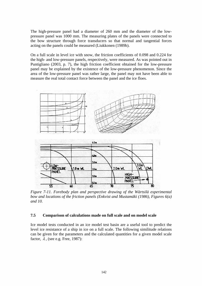
142

The high-pressure panel had a diameter of 260 mm and the diameter of the low-pressure panel was 1000 mm. The measuring plates of the panels were connected to the bow structure through force transducers so that normal and tangential forces acting on the panels could be measured (Liukkonen (1989b). On a full scale in level ice with snow, the friction coefficients of 0.098 and 0.224 for the high- and low-pressure panels, respectively, were measured. As was pointed out in Puntigliano (2003, p. 7), the high friction coefficient obtained for the low-pressure panel may be explained by the existence of the low-pressure phenomenon. Since the area of the low-pressure panel was rather large, the panel may not have been able to measure the real total contact force between the panel and the ice floes.

Figure 7-11. Forebody plan and perspective drawing of the Wärtsilä experimental bow and locations of the friction panels (Enkvist and Mustamäki (1986), Figures 6(a) and 10. 7.5 Comparison of calculations made on full scale and on model scale Ice model tests conducted in an ice model test basin are a useful tool to predict the level ice resistance of a ship in ice on a full scale. The following similitude relations can be given for the parameters and the calculated quantities for a given model scale factor, λ , (see e.g. Free, 1987):

143

3

(the same applies to all length parameters)

.

fsc msc

fsc msc

fsc msc

fsc msc

fsc msc

U U

l l

p p

F F

λλλ

τ λτ

λ

=

=

=

=

=

(7.3)

where the subscript "msc" refers to model scale and "fsc" to full scale. The density, 31000 kg/mρ = and the kinematic viscosity, 31.792 10 Pa sη −= ⋅ ⋅ for water at o0 C cannot be modelled in practice on a model scale and they are the same on a model scale and on a full scale. In order to get some idea about the theoretical error in predicting the resistance of the ice submerging phase resulting from the use of the same fluid properties on a model scale and on a full scale, “computational model tests” were performed by calculating the average pressure and the average shear stress in the gap on a model scale and on a full scale. The model scale factor, λ , was varied from 1 to 30. The parameters used in the calculations on a model scale (see Table 7-3) were calculated using the equations in (7.3). It was assumed that the surface roughness of the ice would be the same on a model scale and on a full scale and, therefore, the minimum distance, hmin, between the hull surface and the ice floe was assumed to be the same in all cases. A value of 0.01 mm was selected for hmin. The same boundary conditions as given in Section 6.1.1.1 were used in the calculations. The flow in the gap is turbulent in the full-scale case, but laminar in all model-scale cases. The average pressure,

1

*dp , and the average shear stress, avτ , in the gap between

the hull surface and the ice floe are given in Table 7-4. The total normal force acting on the ice floe as a result of pressure,

1

*( )p msc dF p lb= , the total normal force resulting

from the static lift of the ice floe, ( )s msc iceF gh lbρΔ= , and the total shear force acting on the ice floe as a result of shear stresses, ( )shear msc avF lbτ= , are also shown in Table 7-4. The difference between the densities of water and ice, ρΔ , was assumed to be 100 kg/m3. Table 7-3. Parameters used in the calculations. Model scale factor , λ

1 (full scale)

5 10 15 20 25 30

l [m] 1.0 0.2 0.1 0.0667 0.05 0.04 0.0333 b [m] 1.0 0.2 0.1 0.0667 0.05 0.04 0.0333 Rx [m] 75 15 7.5 5 3.75 3 2.5 Ry [m] 75 15 7.5 5 3.75 3 2.5 hice [m] 1.0 0.2 0.1 0.067 0.05 0.04 0.033 U [m/s] 5 2.236 1.581 1.291 1.118 1.000 0.912

144

Table 7-4. The results of the calculations. Model scale factor , λ

1 (full

scale)

5 10 15 20 25 30

1

*dp [Pa] -2066.4 -87.4 -80.3 -80.0 -80.4 -80.3 -80.0

avτ [N/m2] 22.9 26.7 30.0 31.0 33.4 35.2 36.6 Fp(msc) [N] 2066.4 3.50 0.80 0.35 0.20 0.13 0.09 Fs(msc) [N] 981.00 7.85 0.98 0.29 0.12 0.06 0.04 Fshear(msc) [N] 22.86 1.07 0.30 0.14 0.08 0.06 0.04 Table 7-5. Full-scale resistance prediction. Model scale factor , λ

1 (full scale)

5 10 15 20 25 30

Fp(fsc) [N] 2066.4 437.1 802.8 1200.0 1607.1 2006.9 2402.0 Fs(fsc) [N] 981.0 981.0 981.0 981.0 981.0 981.0 981.0 Rf(fsc) [N] 304.7 141.8 178.4 218.1 258.8 298.8 338.3 Rshear(fsc) [N] 22.9 133.4 300.0 465.2 668.1 880.0 1098.3 The full-scale resistance prediction and the results of the resistance calculations are shown in Table 7-5 and in Figure 7-12. The forces on a full scale were calculated using the last of the equations in (7.3). The frictional resistance, Rf(fsc), tangent to the hull surface resulting from the normal forces was calculated using the following equation (compare with Equation (1.11)): ( )( ) ( ) ( )f fsc s fsc p fscR F Fμ= + , (7.4) where μ is the friction coefficient. A value of 0.1 was used in the calculations for the friction coefficient. Since the hull geometry is similar on a full scale and on a model scale, the effect of the geometry was omitted in Equation (7.4); compare with Equation (1.11). As expected, the forces caused by shear stress predicted by the calculations made on a model scale are much higher than the forces calculated on a full scale. This is due to the fact that it is not possible to scale down the density and viscosity of water in model tests. This may be one of the reasons why a low friction coefficient is used on a model scale in order to obtain a good correlation of the model test results with results obtained on a full scale (see Liukkonen (1989b)). On the other hand, Figure 7-12 indicates that, according to these calculations, the pressure decrease phenomenon is relatively well modelled in model tests.

145

0

200

400

600

800

1000

1200

0 5 10 15 20 25 30

Model scale factor, л

Res

ista

nce

tang

ent t

o th

e hu

ll su

rfac

e [N

]

Friction force due to normal forces Shear force

Figure 7-12. Comparison of the results of the calculations performed using the full-scale and model-scale values of the parameters. 7.6 Calculation of ice resistance of ships in level ice The interesting question now emerges of whether it is possible to calculate the ice resistance of a ship in level ice. Such an effort could be made by combining the work of Valanto (2001a) and Puntigliano (2003) with the work presented in this thesis. Valanto (2001a) presented the calculation procedure for the ice-breaking and rotative phases and Puntigliano (2003) for the sliding phase. The method presented in this study to calculate the pressure between the hull surface and the ice floes could be incorporated into the model of Puntigliano (2003). The calculation method presented in this study should be amended as follows in order to improve the accuracy of the calculation procedure:

- The finite volume method, as presented by Argir and Frêne (2001), should be used instead of the finite difference method used in this study.

- Triangular-shaped cells should be used in order to be able to model arbitrarily shaped ice floes.

- Different sizes of cells should be used. The calculation procedure presented by Valanto (2001a) can predict the size and form of the broken ice floes, which is a necessary input for the calculation of the ice resistance in the sliding phase. The method should also take into account the possibility of the further breaking of the ice floes, for example as a result of the load induced by the low pressure between the hull surface and the ice floes when they are submerged. The way is open for enthusiastic and hard-working scientists to try to calculate the resistance of a ship in level ice. Finally, it should be mentioned that further research is required to study the effect of snow on level ice resistance. Another interesting topic for research is the effect on level ice resistance of air pressed into the gap between the hull and ice floes by air bubbling systems.

146

7.7 Summary of Chapter 7 In this chapter, the effect of surface roughness on level ice resistance was briefly discussed. The model test results given in Chapter 2 were discussed in the light of the experience gained from the calculations presented in Chapter 6. For several reasons, no calculation of the pressure decrease in the gap between the model surface and the ice floes was possible in most of the cases. For example, the size of the submerged ice floes was not known. Additionally, in most cases the hull form was rather flat, unlike in “normal” convex hull shapes. The analysis given above concerning the observed increase in ice resistance with speed of Segment No. 2 in the model tests of Liukkonen (1989a) indicates that the effect of the change in pressure below the ice floes on ice resistance of Segment No. 2 requires further research. It is possible that the change in pressure below the ice floes in ice model tests is higher than the change in pressure below the model in open water tests. This phenomenon, together with the effect of viscous forces between the model and ice floes, may explain the measured increase of resistance with velocity for Segment No. 2. Some calculations were also presented to explain the model test results obtained for the simplified Waas bow. The calculations indicated that the origin of the measured low pressure in the model tests of Puntigliano (1995) may be the change in the hull geometry when ice floes are submerged by the hull. Although several assumptions had to be made in the calculations in order to get similar results to those in the model tests, the origin of the measured low pressure resulting from the change in the hull curvature seems to explain the phenomenon for this type of hull form qualitatively. It should also be noted that if the magnitude of pressure below the ice floes in ice model tests is different from the magnitude of pressure below the model hull in open water tests, then it is not quite clear how well the pressure measurements in ice reflect the real change of the pressure in the gap between the model surface and the ice floes. This issue could be studied by measuring the water level in the gaps between the segments in model tests in ice and in open water. In addition, calculation of the pressure decrease in the gap between the hull surface and the ice floes for "real" hull surfaces was discussed and the effect of the low-pressure phenomenon on the results of measurements made in friction panel tests was also highlighted. Finally, calculations made with parameters given on a full scale and on a model scale using several model-scale factors were also presented. These calculations indicated that the pressure decrease phenomenon is relatively well modelled in model-scale tests, but the viscous forces cause a considerable error in the results obtained by the model tests.

147

8 Summary The resistance of a ship in level ice as a result of a decrease in pressure between the hull surface and an ice floe when the ice floe is submerged was studied in this thesis. In Chapter 1 three basic phenomena were presented to explain the origin of the change in pressure in the gap between the hull and an ice floe in the sliding phase:



geometry of the hull along the trajectory of an ice floe sliding on the hull. In this study the last two phenomena were studied using the hydrodynamic lubrication theory. For this purpose the Iceflo computer code was developed. In Chapter 2 model- and full-scale data related to the pressure decrease phenomenon were presented. All the model-scale data presented indicate that there is an increase in ice resistance with speed in the sliding phase. The model tests of Liukkonen (1989a) for a two-dimensional model indicate that the normal forces do not increase with speed in the sliding phase, although the ice resistance does increase with speed in the sliding phase. The model tests of Puntigliano (1995 and 2003), both for a two-dimensional model and a cylindrical bow model, even indicate that the normal forces decrease with speed in the sliding phase, although the ice resistance does increase with speed in the sliding phase. These observations, together with the measurements of low pressure in the shear layer between the hull surface and the ice floes, both on a model scale (Puntigliano (1995 and 2003)) and on a full scale (Puntigliano (2000 and 2003)), strongly support the idea that the increase in ice resistance in the sliding phase is due to either the increase in the mechanical friction forces resulting from low pressure in the gap between the hull surface and the ice floes or viscous forces in the gap, or both. In Chapter 3 the governing equations, i.e. the Navier-Stokes equations, were given, the calculation problem was presented, and an outline of the solution methods for the shear-driven motion of fluid between the hull surface and an ice floe in relative motion was given. The preliminary analysis of the flow in the gap, based on the calculation of the Couette Reynolds number and the reduced Reynolds number for the example case, indicated that the calculation method has to be able to model time-dependent laminar and turbulent flow with inertia effects. In Chapter 4 some aspects of the Fluent CFD computer code were described. In order to evaluate the suitability of Fluent for the analysis of the computational problem described in Chapter 3, Fluent was validated against the direct numerical simulation data of Bech et al. (2000) for plane-turbulent Couette flow, and against the experimental data of Nakabayashi (1993) for turbulent Couette-type flow with repeated longitudinal pressure gradients. The conclusion was that Fluent can be used for the calculation of this type of flow.

148

The Iceflo CFD code, based on hydrodynamic lubrication theory with fluid inertia effects, was written to calculate the flow in the gap between the hull surface and an ice floe. Iceflo was verified for a two-dimensional flow against the results calculated by the analytical solution derived by Constantinescu and Galetuse (1974) and validated against the results calculated by the Fluent computer code for the flow between a transversely infinite rotating cylinder and a transversely infinite wall. The code was also verified for a three-dimensional flow against the analytical solution of Kapitsa for the flow between an egg-shaped hull moving above a plane. Verification and validation of Iceflo for a time-dependent flow, i.e. when the gap height changes with time, was done for the analytical solution of two, in a transverse direction, infinitely wide parallel plates approaching or moving away from each other. In all cases the calculated results obtained by Iceflo coincided very well with the analytical solutions and reasonably well with the results obtained by Fluent. In Chapter 6 the flow between an "ball-shaped" hull form and a rectangular ice floe with an area of one square metre was presented. The effect of the boundary conditions at the edges of the ice floe was found to have a very important influence on the results. Optimal computational parameters were studied and the geometric parameters were varied in this chapter. It was found out that the pressure in the gap does not depend very greatly on the minimum distance between the ice floe and the hull surface when the minimum distance between the surfaces is less than 0.1 mm. The effect of the size of the ice floe, the curvature of the hull surface, the velocity of the hull surface, and the inclination angle of the ice floe on the pressure in the gap were also studied in this chapter. The change in the gap geometry with time, the velocity of the hull surface, and the inclination angle of the ice floe had a considerable effect on the pressure in the gap for the geometry considered in the analysis. The analysis confirms that in theory the change in pressure in the gap between the hull and the ice floes may exist as a result of two phenomena: inertia forces or a change in the gap geometry, or both. In Chapter 7 the effect of surface roughness on level ice resistance was briefly discussed. The model test results given in Chapter 2 were discussed in the light of the experience gained from the calculations presented in Chapter 6. For several reasons, no calculation of the pressure decrease in the gap between the model surface and the ice floes was possible in most of the cases. For example, the size of the submerged ice floes was not known. Additionally, in most cases the hull form was rather flat, unlike in “normal” convex hull shapes. The analysis given above concerning the observed increase in ice resistance with speed of Segment No. 2 in the model tests of Liukkonen (1989a) indicates that the effect of the change in pressure below the ice floes on ice resistance of Segment No. 2 requires further research. It is possible that the change in pressure below the ice floes in ice model tests is higher than the change in pressure below the model in open water tests. This phenomenon together with the effect of viscous forces between the model and ice floes may explain the measured increase of resistance with velocity for Segment No. 2. The calculations indicated that the origin of the measured low pressure in the model tests of Puntigliano (1995) may be the change in the hull geometry when ice floes are

149

submerged by the hull. Although several assumptions had to be made in the calculations in order to get similar results to those in the model tests, the origin of the measured low pressure resulting from the change in the hull curvature seems to explain the phenomenon for this type of hull form qualitatively. It should also be noted that, if the magnitude of pressure below the ice floes in ice model tests is different from the magnitude of pressure below the model hull in open water tests, then it is not quite clear how well the pressure measurements in ice reflect the real change of the pressure in the gap between the model surface and the ice floes. This issue could be studied by measuring the water level in the gaps between the segments in model tests in ice and in open water. In addition, calculation of the pressure decrease in the gap between the hull surface and the ice floes for "real" hull surfaces was discussed and the effect of the low-pressure phenomenon on the results of measurements made in friction panel tests was also highlighted in Chapter 7. In Chapter 7 calculations made with parameters given on a full scale and on a model scale using several model-scale factors were also presented. These calculations indicated that the pressure decrease phenomenon is relatively well modelled in model-scale tests, but the viscous forces cause a considerable error in the results obtained by the model tests.

150

9 Conclusions The following two main conclusions can be drawn concerning the origin of the low-pressure phenomenon:

1. The low-pressure phenomenon in the gap between the hull surface and ice floes may be caused by the inertia forces under favourable conditions, as was proposed in Kämäräinen (1993b). However, the existence of this phenomenon requires a continuous shear-driven flow of water in the gap between the hull surface and the ice floes. In this phenomenon the existence of low average pressure in the gap is very sensitive to the position of the ice floes.

2. It is also clear that a change in the hull geometry can be a reason for the existence of low pressure in the gap between the hull surface and ice floes, as was proposed by Enkvist (1972) for convex hull forms and by Puntigliano (2000) for both convex and concave hull forms. The existence of this phenomenon does not require a continuous shear-driven flow of water in the gap between the hull surface and the ice floes.

The following conclusions related to the low-pressure phenomenon can also be drawn:

3. Change of pressure below the ice floes has a negligible effect on ice resistance in the sliding phase, if it is assumed that the pressure below the ice floes has an effect on the pressure above the ice floes through the gaps between adjacent ice floes.

4. Change of pressure below the ice floes should be taken into account in model tests when measurements of resistance of individual segments cut in the transverse direction are evaluated.

5. The low-pressure phenomenon has to be taken into account when the ice resistance of ships in level ice is calculated, since the force resulting from a pressure decrease in the gap between the hull surface and ice floes may be several times higher than the force resulting from the static lift of the ice floes.

6. The low-pressure phenomenon also has to be taken into account in friction panel tests, as was pointed out by Puntigliano (2003).

7. On a full scale the frictional resistance caused by the low pressure in the gap between the hull surface and the ice floes and the static lift of the ice floes is higher than the resistance resulting from viscous forces in the gap.

8. In model-scale tests the viscous forces in the gap between the hull surface and the ice floes may cause considerable error in the full-scale prediction of level ice resistance.

9. Concerning the low-pressure phenomenon, the hull curvature along the ice floe trajectory should be constant and as low as possible in order to avoid decrease of pressure in the gaps between the hull surface and the ice floes when breaking level ice. An inclined cylindrical bow form can be considered to be close to an optimal hull form for this purpose.

151

More research is required on the following topics:

1. There is insufficient knowledge about the boundary conditions at the edges of individual ice floes, as well as the distance of the ice floes from each other in the sliding phase. Model- and full-scale tests should be conducted in order to further investigate this issue.

2. The amount of full-scale data on the low-pressure phenomenon is still quite limited. More tests should be performed on a full scale using different hull forms to further investigate the phenomenon. It should especially be noted that, if the magnitude of pressure below the ice floes in ice model tests is different from the magnitude of pressure below the model hull in open water tests, then it is not quite clear how well the pressure measurements in ice reflect the real change of the pressure in the gap between the model surface and the ice floes. This issue could be studied by measuring the water level in the gaps between the segments in open water tests and in model tests in ice.

3. The effect of snow and slush on level ice resistance requires further studies.

4. The effect of air bubbles in the fluid between the hull surface and the ice floes was not studied in this thesis. This issue also requires further studies.

152

References Anderson D.A., Tannehill J.C. and Pletcher R.H. (1984). Computational Fluid

Mechanics and Heat Transfer. Hemisphere. New York. Arghir M. and Frêne J. (2001). A Triangle Based Finite Volume Method for the

Integration of Lubrication's Incompressible Bulk Flow Equations. Journal of Tribology, January 2001, Vol. 123, 118 - 124.

Bech K.H., Tillmark N., Alfredsson P. and Andersson H.I. (1995). An investigation of

turbulent plane Couette flow at low Reynolds numbers. Journal of Fluid Mechanics (1995), vol. 286, 291-325.

Bech K.H., Tillmark N., Alfredsson P. and Andersson H.I. (2000). Turbulent Plane

Couette Flow. DNS by Bech et al. http://cfd.me.umist.ac.uk/ercoftac/database/cases/case71/cas71_head.html Blazek J. (2001). Computational Fluid Dynamics: Principles and Applications.

Elsevier Science Ltd, 2001. Cameron A. (1976). Basic Lubrication Theory. Ellis Horwood Limited, 1976, Second

Edition. Constantinescu V.N. and Galetuse S. (1965). On the Determination of Friction Forces

in Turbulent Lubrication. ASLE Transactions 8, 367 - 380 Constantinescu V.N. (1970). On the Influence of Inertia Forces in Turbulent and

Laminar Self-Acting Films. Journal of Lubrication Technology, July 1970, 473 - 481.

Constantinescu V.N. and Galetuse S. (1974). On the Possibilities of Improving the

Accuracy of the Evaluation of Inertia Forces in Laminar and Turbulent Films. Journal of Lubrication Technology, July 1974, 69 - 79.

Constantinescu V.N., Galetuse S. and Kennedy F. (1975). On the Comparison

Between Lubrication Theory, Including Turbulence and Inertia Forces, and Some Experimental Data. Journal of Lubrication Technology, July 1975, 439 - 449.

Constantinescu V.N. and Galetuse S. (1982). Operating Characteristics of Journal

Bearings in Turbulent Inertial Flow. Journal of Lubrication Technology, April 1982, Vol. 104, 173 - 179.

Eggert E.F. (1939). Further Form Resistance Experiments. SNAME Transactions

1939, Vol. 47, 303 – 330.

Enkvist E. (1972). On the Ice Resistance Encountered by Ships Operating in the Continuous Mode of Icebreaking. The Swedish Academy of Engineering Sciences in Finland, Helsinki, Report No. 24.

153

Enkvist E. and Mustamäki E. (1986). Model and Full-Scale Tests with an Innovative Icebreaker Bow. SNAME Transactions, Vol. 94, 1986, 325 – 351.

Enkvist E., Varsta P. and Riska K. (1979). The Ship-ice Interaction. Proceedings of

the 5th International Conference on Port and Ocean Engineering under Arctic Conditions, Trondheim, Norway, 977 – 1002.

Ferziger J.H. and Peric M. (2002). Computational Methods for Fluid Dynamics, 3rd

revised edition, Springer-Verlag. Berlin, Heidelberg, New York. Fluent (1998). FLUENT 5 User's Guide. Fluent inc. July 26, 1998. Free A.P. (1987). Solving Icebreaker Design Problems using Ice Model Basins. MTS

Journal, Vol. 21, No.3, 37 – 47. Griebel M., Dornseifer Th. and Neunheffer T. (1998). Numerical Simulation in Fluid

Dynamics. A Practical Introduction. The Society for Industrial and Applied Mathematics.

Harlow F. and Welch J. (1965). Numerical Calculation of Time-dependent Viscous

Incompressible Flow of Fluid with Free Surface. The Physics of Fluids, 8, 2182 – 2189.

Hirs G.G. (1973). Bulk Flow Theory for Turbulence in Lubricant Films, Trans.

ASME, series F, vol. 95, 137 - 146. Holmberg K. (1984). Friction in Low Speed Lubricated Rolling and Sliding Contacts.

Thesis for the degree of Doctor of Technology, Technical Research Centre of Finland, Publications 16, Espoo, April 1984.

Izumiyama K., Wako D. and Uto Sh. (1999). Ice Force Distribution Around a Ship

Hull. POAC'99. Johansson R. (1988). Laser Based Surface Roughness Measurements of Snow and Sea

Ice on the Centimeter Scale. Department of Radio and Space Science with Onsala Space Observatory, Research Report No. 162, 1988.

Kashteljan V.I. and Ryvlin A.,Ya. (1966). Consideration of the Natural

Characteristics of Continuous Ice in Evaluating Its Penetrability by an Icebreaker (in Russian). Problemy Arktiki i Antarktiki, Vol. 22, Leningrad, 75 – 81.

Kashteljan V.I., Ryvlin A.,Ya., Faddeyev O.V. and Yagodkin A.Ya. (1973).

Icebreakers, CRREL Draft Translation 418. Kayo Y. (1993). Measurement of Ice Load Distribution on an Icebreaker Bow Model

Composed by Load Panels. The 12th International Conference on Port and Ocean Engineering under Arctic Conditions (POAC), Hamburg, Volume 1, 328-337.

154

Kivioja S., Kivivuori S. and Salonen P. (2001). Tribologia - kitka, kuluminen ja voitelu (Tribology – Friction, Wear and Lubrication, in Finnish). Otatieto. Oy Yliopistokustannus University Press Finland Ltd, Helsinki 2001.

Kundu P.K. and Cohen I.M. (2002). Fluid Mechanics. Academic Press. Kämäräinen J. (1993a). Evaluation of Ship Ice Resistance Calculation Methods.

Licentiate's thesis. Helsinki University of Technology, Faculty of Mechanical Engineering.

Kämäräinen J. (1993b). On the Speed Dependence of the Ice Submerging Resistance

of Ship Ice Resistance in Level Ice. Helsinki University of Technology, Faculty of Information Technology, Computational Dynamics. Otaniemi 1993/38.

Kämäräinen J. (1994). On the Speed Dependence of the Ice Submerging Resistance in

Level Ice. ISOPE -94, Osaka, Japan, April 10-15, 1994. Launder B.E. and Spalding D.B. (1972). Lectures in Mathematical Models of

Turbulence. Academic Press, London, England. Launder B.E. and Sharma B.I. (1974). Application of the Energy-dissipation Model of

Turbulence to the Calculation of Flow near a Spinning Disk. Letters in Heat and Mass Transfer, Vol. 1, 131-137, 1974.

Launder B.E. and Leschziner M. (1978a). Flow in Finite-Width, Thrust Bearings

Including Inertia Effects, I - Laminar Flow. Journal of Lubrication Technology, Vol. 100, July 1978, 330 - 338.

Launder B.E. and Leschziner M. (1978b). Flow in Finite-Width, Thrust Bearings

Including Inertia Effects, II - Turbulent Flow. Journal of Lubrication Technology, Vol. 100, July 1978, 339 - 345.

Leiviskä T., Tuhkuri J. and Riska K. (2001). Model Test on Resistance in Ice-free Ice

Channels. POAC'01, Ottawa, Ontario, Canada, 881 - 890. Leschziner M. (1976). Turbulent Flow in Finite Width Bearing Films Including

Turbulent Transport and Inertia Effects. Thesis submitted for the degree of Doctor of Philosophy in the faculty of engineering. University of London.

Lindqvist G. (1989). A Straightforward Method for Calculation of Ice Resistance of

Ships. POAC'89, 722-735.

Liukkonen S. (1989a). Jäävastuksen kitka- ja nopeuskomponenteista segmentoidun 2D-mallin kokeissa. Merihydrodynamiikan lisensiaattiseminaari, kevät 1989. (About Friction and Speed Components of a Segmented 2-D Model. Licentiate Seminar on Marine Hydrodynamics, Spring 1989, in Finnish, not published).

Liukkonen S. (1989b). Friction Panel Measurements in Full-Scale and Model-Scale

Icebreaking Ship Tests. Journal of Offshore Mechanics and Arctic Engineering. August 1989, Vol. 111, 251 – 253.

155

Liukkonen S. (1992). Theoretic Approach to Physical Modelling of Kinetic Friction between Ice and Ship. Proceedings of the 11th International Conference on Offshore Mechanics and Arctic Engineering, Volume IV, Arctic/Polar Technology, ASME 1992.

Liukkonen S. and Nortala-Hoikkanen A. (1992). Ice Resistance Tests on a Segmented

Icebreaker Model. IAHR Ice Symposium, Banff, Alberta, Canada. van Manen J.D. and van Oossanen P. (1988). Principles of Naval Architecture,

Second Revision, Volume II: Resistance, Propulsion, and Vibration. Society of Naval Architects and Marine Engineers, Jersey City, New Jersey USA, 1988. E. V. Lewis, Editor.

Nakabayashi K., Kitoh O. and Iwata H. (1991). Turbulent Couette Type Flow with an

Alternating Pressure Gradient. Presented at 8th Symposium on Turbulent Shear Flows, Munich, poster no. I-13.

Nakabayashi K. (1993). Couette Flow with Fixed Wavy Wall. Experiments by

Nakabayashi. http://cfd.me.umist.ac.uk/ercoftac/database/cases/case10/cas10_head.html Nawwar A.M., Howard D. and Bayly I.M. (1984). Segmented Icebreaker Ship Model

Testing Technique Development. The Seventh International Symposium on Ice, Hamburg, West Germany, International Association for Hydraulic Research, 255 - 265.

Ng Ch.-W. and Pan C.H.T. (1965). A Linearized Turbulent Lubrication Theory.

Transactions of the ASME, Journal of Basic Engineering, September 1965, 675 - 688.

Nyman T. (1986). On the Ice-Breaking Component in the Level Ice Resistance. The

Eight International Symposium on Ice, Iowa City, International Association for Hydraulic Research, 113 - 124.

Patankar S.V. (1980). Numerical Heat Transfer and Fluid Flow. McGraw-Hill, New

York. Paterson A.R. (1997). A First Course in Fluid Dynamics. Cambridge University

Press. Pinkus O. and Sternlicht B. (1961). Theory of Hydrodynamic Lubrication. McGraw-

Hill Book Company, Inc., 1961. Puntigliano F.M. (1995). On the Resistance Components Below the Waterline in the

Continuous Mode of Icebreaking - Model Tests. HSVA Report No. E253/95. Puntigliano F.M. (1997). On the Ship Resistance under the Design Waterline in the

Continuous Mode of Icebreaking in Level Ice. OMAE '97, 16th International Conference on Offshore Mechanics & Arctic Engineering, April 13-17, 1997, Yokohama, Japan.

156

Puntigliano F.M. (2000). Ice Performance of the MPV Neuwerk. On the Low Pressure Phenomenon between Ice and Hull, Full-Scale Trials, Physical and Mathematical Modelling. HSVA Report No. 1640 Part B.

Puntigliano F.M. (2003). Experimental and Numerical Research on the Interaction

Between Ice Floes and a Ship's Hull During Icebreaking. TU Hamburg - Harburg Schriftenreihe Schiffbau, September 2003, Bericht 622.

Salonen E.-M. (1987). Mekaniikan käsitteitä ja kaavoja, versio 1, Teknillinen

korkeakoulu, Opetusmoniste No 6, Otaniemi, 1987. (Concepts and Equations of Mechanics, Version 1, Helsinki University of Technology, Lecture Notes No 6, Otaniemi, 1987, in Finnish)

Schlichting H. (1979). Boundary-Layer Theory, McGraw-Hill Book Company. Schlichting H. and Gersten K. (2000). Boundary-Layer Theory, 8th Revised and

Enlarged Edition, Springer. SFS-EN ISO 4287 (1999). Geometrical product specifications (GPS). Surface texture:

Profile method. Terms, definitions and surface texture parameters (ISO 4287:1997)

Smalley A.J., Vohr J.H., Costelli V. and Wachmann C. (1974). An Analytical and

Experimental Investigation of Turbulent Flow in Bearing Films Involving Convective Fluid Inertia Forces, Journal of Lubrication Technology, January 1974, 151 - 157.

Szeri A.Z. (1998). Fluid Film Lubrication, Theory and Design. Cambridge University

Press.

Taylor C.M. (1970). Turbulent Lubrication Theory Applied to Fluid Film Bearing Design. Proc. Instn. Mech. Engrs., 40 - 47.

Truckenbrodt E. (1968). Strömungsmechanik, Springer – Verlag, New York, 1968. Tsoy L. G. and Sinjaev A.K. (1989). The Shallow Draft Nuclear-powered Icebreaker

Taimyr (in Russian), Sudostroenie No. 7, 1989, 6 – 9. Valanto P. (1989). Experimental and Theoretical Investigation of the Icebreaking

Cycle in Two Dimensions. Thesis for the degree of Doctor of Philosophy. University of California at Berkeley.

Valanto P. (1993). Investigation of the Icebreaking Pattern at the Bow of the IB

Kapitan Sorokin on the Yenisei River Estuary in May 1991. Proceedings of the 12th International Conference on Offshore Mechanics and Arctic Engineering. Book No. G00680 - 1993, 127 - 134.

Valanto P. (2001a). The Resistance of Ships in Level Ice. SNAME Transactions, Vol.

109, 2001, 53 – 83.

157

Valanto P. (2001b). On the Cause and Distribution of Resistance Forces on Ship Hulls moving in Level Ice. Port and Ocean Engineering under Arctic Conditions, POAC'01, August 12 - 17, 2001, Ottawa, Ontario, Canada, p. 803 - 813.

White F. (1991). Viscous Fluid Flow, McGraw-Hill, Inc., New York, 1991. Wolfshtein M. (1969). The Velocity and Temperature Distribution of One-

dimensional Flow with Turbulence Augmentation and Pressure Gradient. International Journal of Heat and Mass Transfer, 12, 301-318.

World Meteorological Organization (1981). Sea Ice Information Services in the

World, WMO-No. 574, Secretariat of the World Meteorological Organization – Geneva – Switzerland, 1981.

Zuev V.A. (1986). The Means to Extend the Navigation Season of the Inland

Waterways (in Russian). Leningrad, Sudostroenie, 1986.

ISBN 978-951-22-8860-1ISBN 978-951-22-8861-8 (PDF)ISSN 1795-2239ISSN 1795-4584 (PDF)

THEORETICAL INVESTIGATION ON THE EFFECT OF FLUID …

Documents

Transcript of THEORETICAL INVESTIGATION ON THE EFFECT OF FLUID …