Theoretical Background and Practical Examples
182
1 MOLARIS-XG: Version 9.15 Theoretical Background and Practical Examples Release date: September 28, 2015
Transcript of Theoretical Background and Practical Examples

1
MOLARIS-XG: Version 9.15
Theoretical Background
and Practical Examples
Release date: September 28, 2015

2

Contents
1 Introduction 7
1.1 What is MOLARIS and MOLARIS-XG? . . . . . . . . . . . . . . . . . . . 71.1.1 What is ENZYMIX? . . . . . . . . . . . . . . . . . . . . . . . . . . 91.1.2 What is POLARIS? . . . . . . . . . . . . . . . . . . . . . . . . . . 101.1.3 How to start . . . . . . . . . . . . . . . . . . . . . . . . . . . . . . 13
2 Theory 15
2.1 A background for the methods used in ENZYMIX . . . . . . . . . . . . . . 152.1.1 All-atom models and Force Field methods . . . . . . . . . . . . . . 152.1.2 Free energy perturbation (FEP) calculations . . . . . . . . . . . . . 192.1.3 The Linear Response Approximation . . . . . . . . . . . . . . . . 202.1.4 The division of the system into regions . . . . . . . . . . . . . . . 222.1.5 Spherical boundary conditions . . . . . . . . . . . . . . . . . . . . 242.1.6 Long-range effects and the LRF approach . . . . . . . . . . . . . . 242.1.7 The EVB method . . . . . . . . . . . . . . . . . . . . . . . . . . . 262.1.8 EVB potential surfaces . . . . . . . . . . . . . . . . . . . . . . . . 282.1.9 Evaluating reaction profiles . . . . . . . . . . . . . . . . . . . . . 292.1.10 QM/MM Molecular Orbitals calculations . . . . . . . . . . . . . . 322.1.11 Entropy calculations . . . . . . . . . . . . . . . . . . . . . . . . . 33
2.2 A background for the methods used in POLARIS . . . . . . . . . . . . . . 352.2.1 The use of simplified models and implicit representations . . . . . . 352.2.2 The PDLD model and the meaning of the PDLD regions . . . . . . 372.2.3 The PDLD radii . . . . . . . . . . . . . . . . . . . . . . . . . . . . 392.2.4 The POLARIS charges . . . . . . . . . . . . . . . . . . . . . . . . 402.2.5 Thermodynamic cycle and PDLD free energy contributions . . . . 422.2.6 Averaging PDLD results over protein configurations . . . . . . . . 442.2.7 The semi-macroscopic PDLD/S method . . . . . . . . . . . . . . . 442.2.8 The PDLD-LRA and PDLD/S-LRA methods . . . . . . . . . . . . 47
2.3 Coarse-Grained Model . . . . . . . . . . . . . . . . . . . . . . . . . . . . 482.3.1 Introduction . . . . . . . . . . . . . . . . . . . . . . . . . . . . . . 482.3.2 The MOLARIS CG model . . . . . . . . . . . . . . . . . . . . . . 502.3.3 Electrolyte and Voltage Effect . . . . . . . . . . . . . . . . . . . . 66
3

4 CONTENTS
3 Specific applications and practical aspects 69
3.1 General groups of keywords . . . . . . . . . . . . . . . . . . . . . . . . . 693.2 Running the program and updating the amino acid library . . . . . . . . . . 693.3 Using ANALYZE . . . . . . . . . . . . . . . . . . . . . . . . . . . . . . . 703.4 Using ENZYMIX . . . . . . . . . . . . . . . . . . . . . . . . . . . . . . . 71
3.4.1 Simple MD relaxation of a macromolecule . . . . . . . . . . . . . 713.4.2 EVB calculations . . . . . . . . . . . . . . . . . . . . . . . . . . . 753.4.3 Simulating the PT reaction of Subtilisin . . . . . . . . . . . . . . . 783.4.4 Interpreting the Results of an Enzymix Run . . . . . . . . . . . . . 793.4.5 Simulating the SN2 reaction of Subtilisin . . . . . . . . . . . . . . 843.4.6 Ground state EVB calculations . . . . . . . . . . . . . . . . . . . . 863.4.7 Adiabatic charging (AC) and other FEP calculations . . . . . . . . 863.4.8 Refinement of the EVB parameters . . . . . . . . . . . . . . . . . 873.4.9 QM/MM calculations . . . . . . . . . . . . . . . . . . . . . . . . . 933.4.10 All-atom LRA results . . . . . . . . . . . . . . . . . . . . . . . . . 963.4.11 Restraint Release Approach calculations (RRA) . . . . . . . . . . . 963.4.12 FEP calcaultion of mutating dummy atoms . . . . . . . . . . . . . 100
3.5 Using POLARIS . . . . . . . . . . . . . . . . . . . . . . . . . . . . . . . 1023.5.1 Calculating solvation energies of molecules in water . . . . . . . . 1023.5.2 Calculating solvation free energies using ab initio charges . . . . . 1043.5.3 Solvation energy of a part of a macromolecule . . . . . . . . . . . 1043.5.4 Calculations of pKa’s of ionizable groups in proteins . . . . . . . . 1093.5.5 All-atom LRA calculations of pKas . . . . . . . . . . . . . . . . . 1133.5.6 Titration curves and evaluation of the charges of ionizable residues
as a function of pH . . . . . . . . . . . . . . . . . . . . . . . . . . 1143.5.7 Calculations of ionic strength effects . . . . . . . . . . . . . . . . . 1193.5.8 Redox Potentials of Proteins . . . . . . . . . . . . . . . . . . . . . 1203.5.9 Calculations of binding free energies . . . . . . . . . . . . . . . . 1223.5.10 Ion channels . . . . . . . . . . . . . . . . . . . . . . . . . . . . . 1313.5.11 Calculating electric fields . . . . . . . . . . . . . . . . . . . . . . . 1313.5.12 LD calculations using Chemsol . . . . . . . . . . . . . . . . . . . 132
3.6 Using the CG model . . . . . . . . . . . . . . . . . . . . . . . . . . . . . 1323.6.1 Trimming . . . . . . . . . . . . . . . . . . . . . . . . . . . . . . . 1323.6.2 Run a coarse grained protein relaxation and perform basic calcula-
tions . . . . . . . . . . . . . . . . . . . . . . . . . . . . . . . . . . 1333.6.3 MONTE CARLO (MC) Evaluation of Ionization states . . . . . . . 1363.6.4 Evaluation of absolute folding energies . . . . . . . . . . . . . . . 142
3.7 Effect of Electrolyte and Membrane Potential . . . . . . . . . . . . . . . . 1493.7.1 Introduction . . . . . . . . . . . . . . . . . . . . . . . . . . . . . . 1493.7.2 Input Files Description . . . . . . . . . . . . . . . . . . . . . . . . 1503.7.3 Output files . . . . . . . . . . . . . . . . . . . . . . . . . . . . . . 151
3.8 Langevin Dynamics Simulation of Ion Channels . . . . . . . . . . . . . . . 1523.8.1 Introduction . . . . . . . . . . . . . . . . . . . . . . . . . . . . . . 1523.8.2 Input Files Description . . . . . . . . . . . . . . . . . . . . . . . . 1523.8.3 Output files . . . . . . . . . . . . . . . . . . . . . . . . . . . . . . 156

CONTENTS 5
4 Inverse Keywords 159
4.1 The keywords at different levels . . . . . . . . . . . . . . . . . . . . . . . 1594.2 The keywords split into tasks . . . . . . . . . . . . . . . . . . . . . . . . . 166
5 Appendices 175
5.1 List of Demos . . . . . . . . . . . . . . . . . . . . . . . . . . . . . . . . . 1755.1.1 Demo an_total . . . . . . . . . . . . . . . . . . . . . . . . . . 1755.1.2 Demo ez_relax . . . . . . . . . . . . . . . . . . . . . . . . . . 1755.1.3 Demo ez_EVBgasphase . . . . . . . . . . . . . . . . . . . . . 1755.1.4 Demo ez_EVB . . . . . . . . . . . . . . . . . . . . . . . . . . . . 1755.1.5 Demo ez_EVBcentroid . . . . . . . . . . . . . . . . . . . . . 1765.1.6 Demo ez_EVBadiabgasphase . . . . . . . . . . . . . . . . . 1765.1.7 Demo ez_EVBadiab . . . . . . . . . . . . . . . . . . . . . . . . 1765.1.8 Demo ez_EVBnonequilibrium . . . . . . . . . . . . . . . . . 1765.1.9 Demo ez_PMF . . . . . . . . . . . . . . . . . . . . . . . . . . . . 1765.1.10 Demo ez_AC . . . . . . . . . . . . . . . . . . . . . . . . . . . . . 1765.1.11 Demo ez_RRA . . . . . . . . . . . . . . . . . . . . . . . . . . . . 1765.1.12 Demo pl_solvpdld . . . . . . . . . . . . . . . . . . . . . . . . 1765.1.13 Demo pl_solvfep . . . . . . . . . . . . . . . . . . . . . . . . . 1765.1.14 Demo pl_aipdld . . . . . . . . . . . . . . . . . . . . . . . . . 1765.1.15 Demo pl_bindpdld . . . . . . . . . . . . . . . . . . . . . . . . 1765.1.16 Demo pl_pkapdld . . . . . . . . . . . . . . . . . . . . . . . . . 1765.1.17 Demo pl_pkafep . . . . . . . . . . . . . . . . . . . . . . . . . 1765.1.18 Demo pl_redoxpdld . . . . . . . . . . . . . . . . . . . . . . . 1765.1.19 Demo pl_redoxfep . . . . . . . . . . . . . . . . . . . . . . . . 1765.1.20 Demo pl_logp . . . . . . . . . . . . . . . . . . . . . . . . . . . 1765.1.21 Demo pl_titraph0 . . . . . . . . . . . . . . . . . . . . . . . . 1765.1.22 Demo pl_evbpdld . . . . . . . . . . . . . . . . . . . . . . . . . 176

6 CONTENTS

Chapter 1
Introduction
1.1 What is MOLARIS and MOLARIS-XG?
MOLARIS is a package that integrates two main modules, ENZYMIX and POLARIS, and aset of general utilities which are incorporated in the module ANALYZE. These three mod-ules are interconnected in order to provide a robust and powerful tool for investigating thefunction of biological molecules. The program is particulary effective in studies of enzy-matic reactions [1] and in evaluating electrostatic energies in proteins [2]. MOLARIS-XGis an extension of the MOLARIS package to coarse-grain (CG) calculations [3]. The useand scope of ENZYMIX and POLARIS as well as MOLARIS-XG are described in the nextsections.
Characteristics of the program
The software design principles behind the development of MOLARIS are similar to othermolecular modeling products with the exception that MOLARIS has been developed tobe used by experts and non-experts alike. MOLARIS is a results oriented (as opposed tomethods oriented) product with the following characteristics:
• Targeted to solve a specific R&D problem: Solvation, binding and catalysis.
• Easy to use, to teach, quick to provide results.
• Packaged with the expertise of experienced computational chemists.
• Directly linked to experiments: direct comparison against measured properties.
MOLARISprovides a complete tool for the investigation of the structure-function relation-ships in enzymes and other biomolecules. Thus, MOLARIS can:
• Propagate molecular dynamics (MD) trajectories for various purposes.
• Evaluate free energy profiles for reactions in water and in enzymes, by means ofcombinations of empirical valence bond (EVB) potential energy surfaces with freeenergy perturbation/umbrella sampling (FEP/US) approaches.
7

8 CHAPTER 1. INTRODUCTION
• Obtain solvation free energies of molecules in water or in the protein. Evaluate thesolvation energy of part of a macromolecule. This is done with powerful sphericalboundary conditions and special treatment of long ranged interactions.
• Perform fully automated pKa calculations for ionizable residues in the protein andobtain titration curves of all the residues within the protein. The pKa calculationsare done using the linear response approximation (LRA) method using automaticallygenerated protein configurations for the charged and uncharged states of the givenresidues.
• Obtain absolute binding free energies of ligands - not only enthalpy or scoring func-tions. This again is done with the powerful LRA approach.
• Calculate REDOX potentials in proteins. Here our approach has been shown to beparticularly powerful in very challenging cases including iron sulfur proteins.
• Study ion permeation through ion channels. This allows one to explore the effect ofvoltage on conductance and gating within the actual structure of ion channels.
• Calculate electric fields and molecular electrostatic potentials in proteins.
• Calculate the effect of ionic strength.
• Evaluate entropic effects on binding and obtain activation entropies for enzymaticreactions.
How does MOLARIS differs from other molecular modeling packages?
Some of the above characteristics are shared by MOLARIS and other molecular modelingpackages. However, there are distinctive features in MOLARIS that cannot be found inother programs:
• The use of the EVB/FEP/US approach, which allows one to explore the catalyticactivity of enzymes by means of comparison of the reaction profiles in the enzymeand in solution.
• Proper inclusion of electrostatic effects in water and in proteins, including the treat-ment of induced dipoles by a polarizable force field (which is properly coupled to theEVB Hamiltonian).
• The use of the protein dipoles/Langevin dipoles (PDLD) method and its variants inorder to study solvation and binding energies, REDOX potentials and pKa shifts. Forexample, the PDLD/S-LRA method reliability allows us to obtain accurate bindingfree energies that can be directly compared to experiment.
• The use of proper boundary conditions in free energy calculations, including a uniquerepresentation of the proper solvent polarization on the surface of the simulationsphere. The neglect of this effect leads to problematic results in free energy calcula-tions of charged groups and then the results depend on the size of the group.

1.1. WHAT IS MOLARIS AND MOLARIS-XG? 9
• Proper inclusion of long range effects by means of the local reaction field (LRF)method.
• Advanced FEP treatments of solvation energies and even entropic effects upon ligandbinding or in enzyme catalysis.
1.1.1 What is ENZYMIX?
The main purpose of ENZYMIX is to generate the free energy profile of reactions in solutionand in proteins by means of the EVB/FEP/US methodology. Comparison of the reactionprofile for the solution reaction to that of the enzyme reaction allows the user to differen-tiate between various mechanisms for the enzymatic reaction. Using the EVB method, itis possible to translate a postulated mechanism (e.g., proton transfer, nucleophilic attack,electron transfer, electrophilic attack, etc.) into a force field that the computer can under-stand and can be used for calculating the free energy profile of such a mechanism. Thusthe computer allows the user to simulate the feasibility of a proposed mechanism by com-paring its free energy profile to the profiles of other mechanisms. The use of the ENZYMIXprogram in connection with experimental studies is at present the most powerful way ofstudying reaction mechanisms, of biological macromolecules.
In order to appriciate what is done by ENZYMIX one should realize that it is extremely
hard to generate accurate potential energy surfaces for even small molecules using state-of-the art ab initio techniques. The philosophy behind ENZYMIX is that an alternative tothe elusive ab initio studies of enzymatic reactions is the use of the EVB approach, whichinvolves mixing of valence bond VB type force fields. This EVB approach can be forced toreproduce the ab initio potential energy surface of the relevant reference reaction in solutionand can be used to explore the change of the surface in the enzyme active site. These forcefields are constructed using insights gained from both experimental and theoretical studiesand represent an “engineering” approach to molecular potential surfaces as opposed to the“first principles” approach emphasized in ab initio methods. In this approach we insist ongetting the most reliable experimental or theoretical estimates of the gas phase energiesof the charged fragments. Alternatively, we use the experimental energies of forming thefragments in solution and their calculated solvation free energies, noting that it would beessential to recalibrate the current ab initio results on the same experimental free energies.Since the force fields in ENZYMIX are empirical in nature it is possible to make them moreaccurate as more experimental and/or ab initio-based information is gained. See refs. [1, 4]for further discussion.
In addition to the above EVB/FEP/US tasks, the ENZYMIX module also provides avery effective way of performing a wide range of simulation studies. This includes thespecial ability to perfrom reliable FEP calculations of charges in proteins. This is due tothe special boundary conditions and long range treatments in the program (see sections2.1.5 and 2.1.6). ENZYMIX also allows one to perform advanced QM/MM calculations[5].

10 CHAPTER 1. INTRODUCTION
1.1.2 What is POLARIS?
A quantitative understanding of the properties of molecules in solution is critically impor-tant to biochemistry, medicine, materials and the environmental sciences. POLARIS is acomplete molecular modeling software for the design, simulation, and analysis of molecu-lar properties in solution.
POLARIS provides a powerful tool for calculations of electrostatic properties ofmolecules and macromolecules in solution. All the key factors that determine the energycontributions of molecules in solution - permanent dipoles, induced dipoles, charges, dis-persion terms, and hydrophobicity - are included in POLARIS.
Langevin dipoles in POLARIS accurately model the long term time-averaged polariza-tion of the solvent molecules achieving a very fast convergence in calculations of solvationeffects.
How does POLARIS differ from other molecular modeling programs?
The idea that the electrostatic energy is one of the most important structure-function corre-lators for macromolecules is becoming accepted as a general rule in molecular modeling.Trying, however, to obtain reliable estimates of electrostatic energies in macromolecules isfar from trivial. In principle one can take one of the following three options to model thesystem (see also Figure 1.1):
1. One can use fully microscopic models which represent explicitly all the solventand/or proteins atoms (see refs. [6, 7]). Such approaches, which in fact can beused within ENZYMIX, require very large amounts of computer time and involvemajor convergence problems. Furthermore, simulations that use customary cutoffdistances can give inaccurate results due to incorrect treatment of long range electro-static forces (see discussion in [8, 9, 10]).
2. One can represent the solvent molecules by dipoles that would account for the mainphysics of the solute-solvent interaction.[2]
3. The solvent region can be divided into relatively large volume elements and theaverage polarization of, as well as the average field of, each volume elementcan be treated within the continuum approximation. The system will be thentreated by solving the continuum electrostatic problem by discretized continuumapproaches.[11, 12]

1.1. WHAT IS MOLARIS AND MOLARIS-XG? 11
Options for representing the solvent in computer simulation approaches
Figure 1.1: Illustrating the three main options for representing the solvent in computer simulation approaches.The microscopic model uses detailed all-atom representation and evaluates the average interaction betweenthe solvent residual charges and the solute charges. Such calculations are expensive. The simplified mi-croscopic model replaces the time average dipole of each solvent molecule by a point dipole, while themacroscopic model is based on considering a collection of solvent dipoles in a large volume element as apolarization vector.
The POLARIS program takes the second option using the protein dipoles Langevindipoles (PDLD) approach. This is a simplified microscopic approach that retains the clearphysics of the microscopic world, where one does not have to assume an arbitrary dielectricconstant (the dielectric is just the vacuum dielectric constant). However, the solvent is dras-tically simplified and the time average polarization of each solvent molecule is representedby a Langevin type dipole.[2, 13]
(µLi )n+1 = eni µ0
(
cothχni −1
χni
)
(1.1)
χni =C ′µ0
kBT|ξni | (1.2)

12 CHAPTER 1. INTRODUCTION
where eni is a unit vector in the direction of the local field ξni , C ′ is a parameter, and µ0
is taken as 1.8 D. The equation at the site of the given dipole for the effective Langevindipoles, µL
i , is solved iteratively ((µLi )n+1 is determined by the field ξni from the previous
iteration).A useful alternative is provided by assuming a linear polarization law that replaces the
Langevin equation(µLi )
n+1 = αξn+1i (1.3)
Although this equation can, in principle, lead to over polarization of the solvent moleculesnear highly charged sites, it has been found to behave in a stable way and to converge fasterthan eq. 1.1. The user, of course, has the option to use eq. 1.1 simply by selecting theappropriate keyword in the input file.
The PDLD model does not try to reproduce the exact position of the solvent atoms butplaces the solvent dipoles on a simple spherical grid (see discussion in [14]). In order tounderstand the advantage of using such a simplified solvent model it is useful to considersome of the problems associated with using a brute force all-atom simulation. For example,proteins in the Brookhaven Protein Data Base - fit inside a water droplet 85 Ångstroms indiameter (with the notable exception of hemoglobin and related protein molecules). Such adroplet may contain over 12,000 water molecules. Free Energy Perturbation (FEP) methodsmust explicitly represent all these water molecules. Because each water molecule requires18 degrees of freedom (9 coordinates and 9 momenta) the total number of degrees of free-dom for the water molecules alone is over 200,000. Hence, both large physical memory andgreat speed is required to model these systems with FEP methods. Furthermore, the largenumber of degrees of freedom makes the convergence process extremely slow. On the otherhand, POLARIS models each water molecule as a Langevin dipole, reducing the numberof degrees of freedom from 18 to 3 for each water molecule. In addition, the solution ofthe equations governing the polarization of the Langevin dipoles requires less effort thanthe time integration of the Hamiltonian equations of motion for the molecular dynamicsof water molecules used in FEP approaches. Long equilibration molecular dynamics steps(over the orientation of the water molecules) are avoided by the Langevin dipoles whichare reoriented in a self-consistent manner to respond to short and long range electrostaticeffects caused by the solute molecules and by the Langevin dipoles on themselves.
The microscopic results of the PDLD model might involve convergence difficultieswhich should require extensive averaging over the dipoles configurations. POLARIS pro-vides an implicit way for obtaining stable and usually accurate results by scaling the PDLDresults. The corresponding PDLD/S model uses a “dielectric constant” for the protein re-gion (the meaning of this dielectric constant will be discussed in section 2.2). POLARISalso implements the PDLD/S with the LRA formulation. The resulting PDLD/S-LRAmodel provides more consistent results than those obtained with current descritized contin-uum models.
What properties can be studied with POLARIS?
POLARIS accurately predicts the electrostatic energies of molecules in solution, proteinand other environments. This includes:

1.1. WHAT IS MOLARIS AND MOLARIS-XG? 13
• ∆Gsol: Absolute free energies of solvation
• ∆∆G: Shifts in ∆Gsolcaused by the interaction with the given local environment(e.g., in a protein site)
• ∆Gbind: Estimates of free energies of binding
• ∆Gredox: Redox potentials of proteins
• pKa: Evaluates the pKa’s of ionizable groups in macromolecules
• logP : n-octanol/water partition coefficients
• ∆∆g‡: The change in activation energy upon transfer from water to a given enzymeactive site
These properties are key in examining the functioning of biological molecules, the in-teraction of ionic species in solution, the bio-availability of drugs, the stability of microemulsions, the environmental fate of pesticides, the binding constants (IC50) of substratesto enzymes, the redox potentials in electron transfer reactions in solution, the strength ofbinding between various molecules and polymers in solution, the relative solubility be-tween polar and non-polar media, changes in dissociation constants of acids and bases indifferent molecular environments, shifts in pKa’s of amino acids in the interior and on thesurface of proteins, and many other molecular properties in solution.
1.1.3 How to start
This manual provides a detailed theory section and then a section that outlines differentpractical applications. One way to familiarize yourself with MOLARIS is to move to thereference manual, which gives a quick and practical view of the program.

14 CHAPTER 1. INTRODUCTION

Chapter 2
Theory
2.1 A background for the methods used in ENZYMIX
2.1.1 All-atom models and Force Field methods
Potential Functions (Force field)
Computer modeling of macromolecules is based on using a mathematical description of thedependence of their energy on their structure. Such a dependence is called potential surface.Molecular potential surfaces can be evaluated in principle by using quantum mechanicalapproaches. Such approaches are at present too expensive for effective modeling of largemolecules. Alternatively, one can use the fact that macromolecules are assembled by thesame type of bonds that connect the atoms in small molecules. Thus one can describelarge molecules as a collection of small molecular fragments where the overall potentialsurface is expressed as a sum of contributions from bonded atoms and interactions betweennonbonded atoms. Such a representation is usually done by sets of analytical functions thatpresent an approximation to the true potential surface and are called potential functions orforce fields. The functional forms and parameters of molecular force fields are taken fromstudies of small molecules with the implicit assumption that these functions are transferablefrom small to large molecules. Molecule potential functions are usually given in the form
U(s) = Ub,θ(b, θ) + Uφ(φ) + Unb(r) (2.1)
where s is the vector of internal coordinates composed of b, θ, φ, and r, which are, re-spectively, the vectors of bond lengths, bond angles, torsional angles, and the vector ofCartesian coordinates which are used to evaluate the nonbonded distances. The first termdefines a very deep potential well, and since the molecule stays in most cases inside thiswell (except in extreme cases of bond dissociation), it is reasonable to approximate thispart of the potential surface by its quadratic expansion, which is given by
Ub,θ(b, θ) =1
2
∑
i
Kb,i(bi − b0,i)2 +
1
2
∑
i
Kθ,i(θi − θ0,i)2 + cross terms (2.2)
where U is usually given in kcal/mol, b in Å and θ in radians. The torsional potential Uφ isa periodic function, which can be described by the leading terms in the Fourier expansion
15

16 CHAPTER 2. THEORY
of the potential
Uφ =1
2
∑
i
Kφ,i(1− cos nφi) (2.3)
The nonbonded potential, Unb, can be described by an atom-atom interaction potential ofthe form
Unb =∑
ij
Aijr−12ij −Bijr
−6ij + Cqiqj/rij + Uind(r) (2.4)
where rij is the distance between the indicated atoms, the qi’s are the residual atomiccharges, and Uind is the many body inductive effect of the electronic polarizabilities. Theintroduction of potential functions opens the way for the use of computers in conforma-tional analysis (e.g. ref. [15, 16, 17]). The earliest use of potential functions in modelingproteins has been reported by Levitt and Lifson [18].
The accuracy of the given set of potential functions depends, of course, on the specificset of parameters (the Kb, Kθ, A, B, etc.). These parameters can be optimized by usingthem to calculate different independent molecular properties (e.g., energies, structures, andvibrations) and then fitting the calculated properties to the corresponding observed prop-erties by a systematic change of the potential parameters in a least-squares procedure (seeref. [17]).
Simulation of macromolecules must reflect solvent effects which are not just smallperturbations but major contributors to the overall energetics and force. In fact, modeling ofmacromolecules in a vacuum is quite irrelevant as much as the behavior of such moleculesin solution and proteins is concerned. Here, one can use all-atom solvent models [19, 20,21] or simplified solvent models (e.g., ref. [2]) as a part of the overall potential function.One can also use implicit solvent models (e.g., ref. [22]).
Molecular Mechanics
The modeling of the properties of molecules using the corresponding potential functions iscalled molecular mechanics (MM). This name reflects the fact that a molecular force fieldconsiders a molecule as a collection of balls connected by springs and that examination ofthe mechanical properties of such a system is similar to the study of the properties of thecorresponding molecule.
The MM approaches involve several techniques that are aimed at determining differentmolecular properties. In particular, with a given set of analytical potential functions one canevaluate the molecular equilibrium geometries and the vibrations around these configura-tions. The task can be accomplished in the simplest way using the Cartesian representation.That is, the potential surface for a molecule with n atoms can be expanded formally aroundthe equilibrium configuration r0 and give
U(r0 + δr) = U(r0) +∑
iα
(
∂U
∂riα
)
δriα +∑
iα,jβ
(
∂2U
∂riα∂rjβ
)
δriαδrjβ + · · · (2.5)
where the indices i and j designate atoms while α and β run over the x, y, and z coordinatesof each atom. The first term is just the energy of the molecule at the equilibrium geometry.The second and third terms can be used (see below) to evaluate the equilibrium geometry
2.1. A BACKGROUND FOR THE METHODS USED IN ENZYMIX 17
and the vibrational frequencies. Equation 2.5 and the following paragraphs are written inCartesian coordinates.
The first term in eq. 2.5 is just the energy of the system at equilibrium. The second termrepresents the deviation from the equilibrium and the 3n set of equations (for i = 1, 2, . . . nand α = x, y, z )
∂U
∂riα= 0 (2.6)
represents the condition that r0 is an equilibrium configuration.The second and third terms in Eq. 2.5 can be used in locating the minima on the
potential energy surface and in finding the corresponding equilibrium geometries. One ofthe most effective methods is the modified Newton-Raphson method [23, 17]. This methodis based on expanding the gradient as a Taylor series around the given r and finding the δrthat leads to r0 where the gradient is zero (i.e. r0 = δr). This gives
∂U(r0)
∂riα=∂U(r0 + δr)
∂riα+∑
jβ
Fiα,jβδrjβ = 0 (2.7)
where F is the matrix of second derivatives, i.e., Fiα,jβ = ∂2U/∂riαrjβ. Then, solving eq.2.7 one obtains
r0 = r + δr = r − F+∇U(r) (2.8)
where ∇U(r) is the gradient vector and F+ is the generalized inverse of F, which is con-
structed by "filtering" the zero eigenvalues of F before inverting this matrix. The use ofthis approach in molecular studies was introduced in ref. [17].
Equation 2.8 requires the evaluation of the second derivative matrix F, which is quiteinvolved. Alternatively, one can use the conjugated gradient methods where an approxi-mation of F+ is being built while searching the minimum using only the first derivativesvector ∇U (for a description of these powerful methods and related approaches see ref.[23]).
Although the conjugated gradient and related methods are very effective in finding local
minima, they do not overcome the problems associated with the enormous dimensionalityof macromolecules. That is, in systems with many degrees of freedom we expect to finda very large number of local minima and it is not clear, for example, how to find in anefficient way the lowest minimum. For this purpose one must use much more computertime and different types of search procedures (Monte Carlo or molecular dynamics), gen-erating different configurations at different regions of the conformation space and locatingthe minimum energy structure of each region.
Molecular Dynamics
Molecular Dynamics (MD) simulations evaluate the motion of the atoms in a given systemand provide the positions or trajectory of these atoms as a function of time. The trajectoriesare calculated by solving the classical equation of motion for the molecule under consid-eration. This is not unlike the well known approach by which one evaluates the speed andposition of a projectile starting from the initial velocity, the mass and the forces by using

18 CHAPTER 2. THEORY
Newton’s equation of motion. However, in the case of molecules, one obtains the rele-vant forces on each atom from the first derivatives of the given potential functions. Theactual evaluation of classical trajectories is done numerically, expressing the changes incoordinates and velocities at a time increment, ∆t, by
ri(t +∆t) = ri(t) + ri∆t (2.9)
ri(t+∆t) = ri(t) + ri∆t = ri(t)−1
mi
∂U
∂ridt (2.10)
where the dot designates a time derivative and we use Newton’s law:
miri = Fi = −∂U
∂ri(2.11)
starting with a given set of initial conditions [e.g. with the values of ri(t = 0) and ri(t =0)], we can evaluate either by numerically integrating eqs. 2.9 and 2.10 or by using thesomewhat more complicated but far better approximation[20]
ri(t+∆t) = ri(t) + ri(t)∆t+ [4ri(t)− ri(t−∆t)]∆t2/6 (2.12)
This equation allows one to obtain much more accurate results than those of eq. 2.9, usingthe same ∆t’s.
The propagation of classical trajectories of the atoms of a given system corresponds to afixed total energy (determined by the specified initial conditions). However, the evaluationof statistical mechanical averages implies that the system included in the simulation is apart of a much larger system (ensemble) whose atoms are not considered in an explicitway. Thus, in order to simulate a given macroscopic property at a specified temperaturewe must introduce some type of "thermostat" in the system that will keep it at the giventemperature. This can be easily accomplished by assuming equal partition of kinetic energyamong all degrees of freedom. Since each atom has three degrees of freedom with kineticenergy of 1
2mr2 = 3
2kBT (where kB is the Boltzmann constant) we obtain:
T =
∑
imir2i
3nkB(2.13)
where n is the number of atoms in our system. In general, we can adjust the temperatureduring the simulation by scaling the velocities. That is, when T is smaller than the targettemperature we can scale r uniformly by (1+ ε) until the target temperature is obtained. IfT is higher than the target temperature, then a scaling of (1−ε) is used. More sophisticatedconsiderations for constant temperature simulations are described elsewhere[20].
The strength of MD approaches is associated with the fact that they have the abilityto simulate, at least in principle, the true microscopic behaviors of macromolecules. Theweakness is associated with the fact that some properties reflect extremely long time pro-cesses which cannot be simulated by any current computer.
The emergence of MD simulations in studies of biological systems can be traced to asimulation of the dynamics of the primary event in the visual process [24] that correctlypredicted a photoisomerization process of around 100 femptoseconds. A subsequent study

2.1. A BACKGROUND FOR THE METHODS USED IN ENZYMIX 19
[25] attempted to examine the heat capacity of BPTI by a very short simulation of thisprotein in vacuum. However, at the early stages of the development of this field, it wasnot possible to obtain meaningful results for average properties of macromolecules due tothe need for much stronger computers to reach a reasonable convergence (the heat capacityis drastically underestimated [26], reflecting artificial relaxation motions). Nevertheless,ultrafast reactions such as those that control the photobiological process could be simulatedeven at this early stage [24].
Eventually with the increase of computer power it has become feasible to reach simu-lation times of nanoseconds and to start to obtain meaningful average properties of macro-molecules.
The time needed to reach accurate results for average properties depends on the modelused and number of local minima. For example, models that trim the protein to a spherewith the proper spherical boundary conditions [10] converge much faster than models thatinvolve periodic boundary conditions [27] since the latter involves more molecules andmore minima. As much as accuracy is concerned, the proper treatment of long-range effectsis crucial and improved convergence is usually associated with more proper treatment oflong-range forces [13].
MD simulation methods provide a powerful way of evaluating average properties suchas free energies but it must be emphasized that such properties have little to do with dy-namics per se and can be evaluated by other averaging approaches such as Monte Carlomethods. Similarly, the most important factors that determine the rate constants of mostbiological processes do not reflect dynamical properties but rather the probability of reach-ing the transition state configuration (see ref. [4]). Nevertheless, in cases of light inducedultra-fast photobiological processes, there are probably important effects that can be con-sidered as dynamical properties and MD simulations provide a direct way of modeling sucheffects.
2.1.2 Free energy perturbation (FEP) calculations
With a given set of potential functions one can simulate experimentally observed macro-scopic properties using microscopic models. According to the theory of statistical mechan-ics, one should consider all the quantum mechanical energy levels of the system in orderto evaluate different average properties[28]. However, in the classical limit it is possible toapproximate the average of a given property, A (which is independent of the momentum ofthe system), by[28]
〈A〉 =1
z(U)
∫
A(r) exp{−U(r)β}dr (2.14)
z(U) =
∫
exp{−U(r)β}dr (2.15)
where dr designates the volume element of the complete space spanned by the 3n vector rassociated with the n atoms of the system. The evaluation of Eq. 2.14 requires us to exploreall points in the entire configuration space of the given system. Such a study of solvatedmacromolecule is clearly impossible with any of the available computers. However, onecan hope that the average over a limited number of configurations will give similar results

20 CHAPTER 2. THEORY
to those obtained from an average over the entire space. With this working hypothesis wecan try to look for an efficient way of spanning phase space.
Evaluation of free energies by statistical mechanical approaches are extremely timeconsuming due to sampling problems. Fortunately, it is possible in some cases to obtainmeaningful results using perturbation approaches. Such approaches exploit the fact thatmany important properties depend on local changes in the macromolecules so that the effectof the overall macromolecular potential cancels out. Such calculations are usually doneby the so-called free-energy perturbation (FEP) method [29, 30] and the related umbrellasampling method [30]. This method evaluates the free energy associated with the changeof the potential surface from U1 to U2 by gradually changing the potential surface using therelationship
Um(λm) = U1(1− λm) + U2λm (2.16)
The free-energy increment δG(λm → λm′) associated with the change of Um to Um′ to canbe obtained by [30]
exp{−δG(λm → λm′)β} = 〈exp{−(Um′ − Um)β〉m (2.17)
where 〈〉m indicates that the given average is evaluated by propagating trajectories overUm.The overall free energy change is now obtained by changing the λm in n equal incrementsand evaluating the sum of the corresponding δG:
∆G(U1 → U2) =
n−1∑
m=0
δG(λm → λm+1) (2.18)
The FEP approach has been used extensively in studies of free energies of biologicalsystems (e.g., refs. [19, 31]). It must be emphasized here that the convergence of FEPapproaches is quite slow and that obtaining meaningful results requires proper treatment oflong-range effects (see below).
2.1.3 The Linear Response Approximation
FEP calculations of solvation free energies or related properties for large cofactors or lig-ands are expected to converge extremely slow. A promising strategy may be provided byexploiting the fact that electrostatic effects in solutions (and probably proteins) seem to fol-low the linear response approximation (LRA). Our derivation of the LRA method is basedon studying the functions that describe the free energies of the reactant (a) and product (b)states. These free energy functions (the gα’s of Fig. 2.2) are parabolas of equal curvature inthe macroscopic continuum model where the LRA is assumed, rather than obtained. In thislimit the gα’s are the macroscopic Marcus’ parabolas. In microscopic molecular systemsthe gα’s are defined by[32, 33]
ga = −β−1 lnPa(X) (2.19)
gb = −β−1 lnPb(X) + ∆Ga→b
where X is the generalized reaction coordinate defined by the difference between the po-tential surfaces of state a and state b (X = Ua − Ub).

2.1. A BACKGROUND FOR THE METHODS USED IN ENZYMIX 21
Figure 2.1: copy from [7].

22 CHAPTER 2. THEORY
Figure 2.2: Showing the free energy functions of the reactant and product states, [ga(X) and [gb(X), as twoMarcus’ type parabolas of equal curvature. The solvent reorganization energies at the minima of ga and gbare given by λb = 〈Ub − Ua〉a −∆Ga→b and λa = 〈Ua − Ub〉b +∆Ga→b. By assuming λa = λb one canobtain the LRA estimate of ∆Ga→b (see text and ref. [34]).
For a system that obeys the linear response approximation and has the same ‘solventforce constant’ in the initial and final states, one finds
λ = 〈Ua − Ub〉a +∆Ga→b = 〈Ua − Ub〉b +∆Gb→a (2.20)
Using this equation, we obtain
∆Ga→b =1
2(〈Ua − Ub〉a + 〈Ua − Ub〉b) (2.21)
This equation converges in the case of a single ion (where Ua = 0) to the familiar resultof ∆G = 1
2〈Ub〉b which is, of course, consistent with the corresponding continuum results.
The microscopic validity of the LRA was stablished in [32, 35, 36, 33] and subsequentstudies, and the general result of Eq. 2.21 was introduced in ref. [8] (for an excellentdiscussion, see [37]). This equation has been found to provide a powerful way of estimatingthe results of FEP calculations of large solutes and drugs (see binding section).
2.1.4 The division of the system into regions
Calculations of enzymatic reactions and other processes where electrostatic effect are im-portant present a major challenge. In fact, many seemingly reasonable treatments can giveentirely incorrect electrostatic energies. The main problem is associated with the long-range nature of the electrostatic effect and the fact that one cannot include an infinite sys-tem in simulation studies. Exploiting extensive experience with microscopic simulation ofelectrostatic effects we divided the simulation system to the regions shown in Fig. 2.3.
The system includes the reacting part (region I) which is used in all FEP calculations.The surrounding unconstrained protein (IIa), unconstrained water (IIb), constrained protein(IIIa) and constrained water (IIIb). In addition to these regions which where described

2.1. A BACKGROUND FOR THE METHODS USED IN ENZYMIX 23
+ -(I)
(I)(I)
(Va) bulk
(IIIa)
(IIIb)
(IIa)
(IV)
(IIb)
(Vb)
Figure 2.3: Describing the protein regions in ENZYMIX. Region I contains the reacting atoms (for EVB orAC calculations). Region IIa and IIb are, respectively, the unconstrained protein and water regions. RegionIIIa contains the protein atoms which are constrained to the corresponding X-ray positions (this regiong istreated as a bulk with the dielectric constant of water). Region IIIb contains the surface water and region IVcontains a grid of Langevin dipole. The radius of Region IIIa is determined automatically by the radius ofthe Langevin grid.

24 CHAPTER 2. THEORY
in early studies we surround the system by a grid of Langevin type dipoles (region IV)and then surround the resulting system by a continuum with a dielectric constant of water(region V). When the radius of region IV is smaller than the radius of the complete proteinwe find it useful to trim the protein to the same radius (this gives more stable electrostaticenergies).
2.1.5 Spherical boundary conditions
The time needed to reach accurate results for average properties depends on the modelused and number of local minima. For example, models that trim the protein to a spherewith the proper spherical boundary conditions [10] converge much faster than models thatinvolve periodic boundary conditions [27] since the latter involves more molecules andmore minima.
In particular, ENZYMIX incorporates the Surface-Constrained All-Atom Solvent(SCAAS) model[2, 7, 21]. Thids approach emphasizes the electrostatic constraint, forc-ing the polarization and compression of the finite simulation system, in response to thefield due to internal charges, to approximate the polarization expected from an infinite sys-tem. The treatment focusses on obtaining a reliable treatment of long-range forces (see Fig.2.3). See refs. [21, 13] for a complete description of the method.
2.1.6 Long-range effects and the LRF approach
One of the major problems in molecular dynamics simulations of polar fluids or macro-molecular systems is the evaluation of electrostatic interactions. A system of N atoms de-mands an amount of work proportional to N2 for such calculations. Truncation proceduresthat neglect a significant part of the long-range effects are often necessary for computa-tional feasibility, though such procedures may introduce serious errors in the simulations.MOLARIS introduces a simple and very effective approach for treating the long-range elec-trostatic forces. This method, also called the local reaction field (LRF) method, followssome of the ideas of the previously developed generalized non-periodic Ewald method [38]but then develops into a much simpler method. This is done by dividing the system intoM groups of atoms and evaluating separately the short- and long-range contributions to thepotential of each group. The short-range potential is evaluated explicitly as in any standardtruncation method, while the long-range potential is approximated by the first four termsin a multipole expansion. Furthermore, at the limit of very large systems, the speed of thismethod can be 2 orders of magnitude faster than that of the no-cutoff method even wheneach group contains only a small number of atoms. The LRF method gives much bet-ter results for electrostatic energies in proteins than those obtained by truncation methods.The stability and speed of the local reaction field method provides a powerful tool for themicroscopic evaluation of electrostatic energies in macromolecules.
The LRF method is discussed in ref. [8] and only the main points are emphasizedhere. The development of the LRF method was inspired by the generalized non-periodicEwald method[38]. A precise description of the long-range potential by the extended Ewaldmethod requires the evaluation of many terms in the expansion potential. Furthermore, in

2.1. A BACKGROUND FOR THE METHODS USED IN ENZYMIX 25
the general case one may need to use many expansion centers in order to obtain accu-rate results. Considering this problem, we introduced[8] a variant of the extended Ewaldapproach, whose basic ideas are:
• The N charges of the system are divided into M groups (typically electroneutralgroups), and
• the electrostatic potential at the αth charge of the ithgroup is divided into a short- andlong-range potentials, i.e.,
Φ(rαi ) = Φl(rαi ) + Φs(r
αi ) (2.22)
where r is the vector of the position of the charges.
The short-range potential is simply the sum of the electrostatic contributions from thegroups inside the cutoff Rcut i.e.,
Φs(rαi ) =
∑
j
∑
β
qβj
rαβij+∑
α′ 6=α
qα′
i
rα′α
ii
when (Rij < Rcut) (2.23)
when rαβij is the distance between the αth charge of the ith group and the βth charge of thejth group and Rij is the distance between the centers of the ith and jth groups (the center ofthe ithgroup is taken as Ri =
∑α r
αi qαi∑
α qαi
). The long-range potential is given by
Φl(rαi ) =
∑
j
∑
β
qβj
rαβijwhen (Rij ≥ Rcut) (2.24)
With a large enough Rcut, we can approximate Φl(rαi ) by an expansion potential with
only a few terms. To obtain accurate results, we allow each of the M groups of the systemto form a local expansion center so that each group can be considered as a center for areaction-field-type treatment (see below). For example, in the water system depicted inFig. 2.4, we consider each water molecule as a group. In this case, the interaction betweenwater 1 and water 2 is included in Φs, while that between 1 and 3 is included in Φl. Thetotal Φl for each water molecule represents the effect of all the molecules outside Rcut.
The expansion potential Φ′l used to approximate the Φl of Eq. 2.24 involves the first
four terms in a Taylor series about the center of each group. The long-range electrostaticenergy of the ith group can now be written as an expansion including the monopole, dipole,quadrupole, and octopole moments about the center of the ith group[8]. The total energy ofthe system is now given by
Utotal =1
2
∑
i
∑
α
qαi [Φl(rαi ) + Φs(r
αi )] + UvdW + Ubonding (2.25)
where Ubonding is the bonding interaction between the different fragments of the system de-scribed by the standard ENZYMIX force field and UvdW is the nonelectrostatic van derWaals interaction evaluated within the given Rcut. The contribution from the induced

26 CHAPTER 2. THEORY
Rcut
12
3
Figure 2.4: A schematic picture of a system of water molecules illustrating the basic idea behind the LRFmethod. Each group in this case is a water molecule and its center forms a local expansion center for thelong-range potential in the LRF method. Thus, for example, the Coulombic potential at the oxygen atom ofmolecule 1 is a sum of a short-range potential due to the groups inside the shaded circle (e.g., molecule 2)and a long-range potential due to the groups outside the shaded circle (e.g., molecule 3).
dipoles of the system can also be considered and treated as a part of the electrostatic po-tential. Molecular simulation studies require one to evaluate the forces in addition to theenergy. In our method the long-range force fl acting on a charge q located at ri (near Rj) isgiven by minus the gradient of the corresponding potential energy. The order of the presentmethod is ∼ N × [M×q
L+ P ], where N is the number of charges in the system, P is the
average number of atoms within the cutoff region, and q is related to the number of termsin the expansion potential. Finally, L is the number of time steps in the simulation.
2.1.7 The EVB method
The EVB (Empirical Valence Bond) method[39] is a simple and effective way of includingquantum mechanics into a FEP/MD simulation. This is very important since the model-ing of chemical reactions requires a quantum mechanical treatment. The ability of bondsto move around during a reaction implies that there are more degrees of freedom in thechemical reaction than just the position of the nuclei.
The program ENZYMIX represents the potential energy surfaces of proteins by a com-bination of a classical empirical force field and a quantum empirical valence bond forcefield. The classical force field is used to simulate the parts of the protein removed fromthe actual chemical reaction being studied since there is no bond breaking or making inthis region and the classical force field is extremely well suited for the representation ofmolecules that are not undergoing chemical transformations. In the small region of theprotein where there is a chemical reaction taking place, a quantum mechanical empirical

2.1. A BACKGROUND FOR THE METHODS USED IN ENZYMIX 27
method is used to represent the changing electronic (as opposed to nuclear) coordinatesof the atoms involved in the reaction. A valence bond formalism is used to simulate thereacting atoms since this method is well suited to model bond making and breaking (themolecular orbital method is better suited for the calculation of spectroscopic properties ofmolecules) and the empirical nature of the force field allows calibration of the model toaccurately reproduce experiments.
The ground state potential energy surface (PES) is constructed by mixing (in a quantummechanical sense) the properties of the different valence bond (VB) resonance structuresthat describe the chemical reaction that is taking place. Typically, the user will define areactant and a product bonding pattern for the reaction that he/she is interested in and theEVB method allows the program to determine the energies and forces acting on the atomsthat the user defines as quantum atoms as a function of not just the coordinates of the atomsin space but the percent character of the reactant and product wave function in the actualwave function of the system. This dependence of the force field of the quantum atoms onthe reactant and product character of the system allows the user to cause the reaction tooccur by slowly forcing the system to move from 100% reactant to 100% product wavefunction. As the quantum atoms are forced to react, the protein environment will attemptto “follow” the reaction and it is possible to use the free energy perturbation formalism todetermine the change in the overall free energy of the whole system (Protein + ReactingAtoms + Water) that the user is interested in. For further reading see refs. [1, 40].
The best way to understand this section is through an example. Here we have chosenthe CH3−O− attack on a peptide C=O group, which represents the attack of a methoxy ionon the carbonyl carbon of a peptide group in the substrate of trypsin. In this example thesystem being studied and the two relevant states are shown in Fig. 2.5. To simulate this
Figure 2.5: VB structures for a carbonyl attack to a peptide C=O group
process the user must first define the quantum atoms in the problem. Quantum atoms areany atoms that undergo a change in their bonding pattern as the reaction progresses. In thisexample the quantum atoms are the two oxygen atoms (O2 and O4) and the carbon atom(C3) that is attacked. When the user defines the quantum atoms he/she must also definethe type of the atoms in each resonance form and their charge in each resonance form.After a little thought and preferably some ab initio calculations in solution we can selectthe optimal charges. In the present case one can use the charges in Table 2.1. Of course theuser can modify those parameters in order to fit the EVB surface to ab initio results and/orexperimental data.
Next the user must define the bonding pattern in each of the resonance forms. In reso-

28 CHAPTER 2. THEORY
Resonance Form I Resonance Form IIAtom Type Charge Type Charge
O2 O0 -1.0 O0 -0.2C3 C0 +0.3 C0 +0.2O4 O0 -0.3 O0 -1.0
Table 2.1: Selection of charges for the resonance structures in Fig. 2.5. The atom types refer to the atomtype in the EVB library file evb.lib. The parameters for the EVB atoms are taken from the EVB librarycorresponding to the defined atom type (see the reference manual for more details).
nance form I there is a bond between atom C3 and O4 and in resonance form II there arebonds between atoms O2 and C3 and between atoms C3 and O4.
2.1.8 EVB potential surfaces
Once the user has defined the quantum atoms and their bonding patterns in each of theresonance forms, the program will automatically compute the parameters of the EVB forcefield that defines the interactions of the atoms in each of the resonance forms. This forcefield consists of Morse potentials between atoms that are bonded and repulsive potentialsbetween atoms that are not bonded. Also included are potential functions for angles be-tween bonds containing quantum atoms and torsional potentials around quantum bonds.ENZYMIX uses two different force fields, one for atoms in region I (or EVB region) andone for the rest of the atoms that are treated explicitly (see section 2.1.1). In the aboveexample we will have
ε1 = ∆M(b34) + α(1) + U(1)strain + U
(1)nb (r23) + U
(1)nb (r24) + U
(1)S,s (2.26)
ε2 = ∆M(b23) + ∆M(b34) + α(2) + U(2)strain + U
(2)S,s
Where the M(b) term is the Morse potential for the indicated bond. αiis the energy offorming the indicated resonance form at infinite separation between its fragments, relativeto the minimum value of ε1. The leading terms in Ustrain are given by:
U(1)strain =
1
2
∑
l
K(1)b (b
(1)l − bl0)
2+1
2
∑
m
K(1)θ (θ(1)m − θm0 )
2+1
2
∑
l
K(1)χ (χ(1) − χ0)
2 + ...
U(2)strain =
1
2
∑
l
K(2)b (b
(2)l − bl0)
2+1
2
∑
m
K(2)θ (θ(2)m − θm0 )
2 + ... (2.27)
Where the quadratic bonding terms describe all bonds not represented by the Morse po-tentials and the θ terms represent the angle bending relative to the unstrained equilibrium(120o for the sp2 hybridization of resonance form I and 109.5o for the sp3 hybridizationof resonance form II). Kx is the out of plane force constant for deforming a planar sp2
carbon. There are additional terms which are not discussed here for simplicity.Unb represents electrostatic and repulsion interactions between nonbonded quantum atomsand US,s represents the complicated interaction between the quantum atoms and theremainder of the protein and water atoms (see ref. [41]) for a detailed description of the

2.1. A BACKGROUND FOR THE METHODS USED IN ENZYMIX 29
force field).
The actual potential energy surface of the EVB system is computed by a weighted sumof the potentials of resonance forms I and II. The actual ground state potential is given,in the 2 RS case, by Eg = c21ε1 + c21ε2 + 2(c21c
22)
1/2H12, where the ci’s are determined bydiagonalizing the Hamiltonian:
H =
(
ε1 H12
H12 ε2
)
(2.28)
The off-diagonal element H12 are represented by analytical functions, e.g.,
H12 = A exp{−µR} (2.29)
as described in the refs. [1, 42, 41]. Of course the EVB treatment is not limited to tworesonance structures (e.g., see ref. [39]).Note: The matrix elements are all complicated functions of the nuclear coordinates of theprotein and must be constantly reevaluated during the course of the dynamics simulation.
2.1.9 Evaluating reaction profiles
Since enzymatic reactions occur on time scales much greater than those accessible bymolecular dynamics simulations (most enzymatic reactions have rates on the order if 1-106 sec−1 and molecular dynamics simulations cannot access times over 10−10 sec) it isnecessary to find some way of causing the reaction to happen.
The EVB approach evaluates the activation energy ∆g‡ by running series of trajectorieson potential surfaces that drive the system gradually from one VB state to another. In thesimple case of two VB states, these "mapping" potentials, εm, can be written as linearcombinations of the reactant and product potentials, ε1 and ε2:
εm = (1− λm)ε1 + λmε2 (0 ≤ λm ≤ 1) (2.30)
where λ is changed from 0 to 1 in fixed increments (m = 0, 1, 2, . . . , N).Using the FEP method (section 2.1.2) we have:
δG(λm ⇒ λm′) = −(1
β)ln[< exp(−εm′ − εm)β >m] (2.31)
∆G(λn) = ∆G(λ0 ⇒ λn) =
n−1∑
m=0
δG(λm ⇒ λm+1) (2.32)
where <>m is a configurational average of the quantity in the brackets as the entire sys-tem moves on the potential surface defined by εm. The corresponding free energy profile∆G(λ) of the reaction in solution is shown in Figure 2.6.
The free energy functional ∆G(λ) reflects the electrostatic solvation effects due tochanges of solute charges and intramolecular effects in going from ε1 to ε2. ∆G(λ) is

30 CHAPTER 2. THEORY
Figure 2.6: The mapping free energy, ∆G, for the reaction of the attack of O− to C=O
∆ε (kcal/mol)
∆g (
kca
l/m
ol)
-66.00 -22.00 22.00 66.00
3.30
6.60
9.90
13.20
Figure 2.7: The ground state free energy surface for the O−C=O⇒O-C-O− reaction. Note: The free energyis plotted as a function of the energy gap, ∆ε, which is taken as the reaction coordinate.

2.1. A BACKGROUND FOR THE METHODS USED IN ENZYMIX 31
the potential of mean force due to moving the system from the reactant to the product stateon mapping potential εm.
To calculate the activation free energy ∆g‡ we need to evaluate the probability of beingat the transition state on the actual ground state potential surface. This procedure (whichis described in detail in refs. [32, 42]) divides the coordinate space into subspaces S witha constant value of the energy gap ∆ε = ε2 − ε1 so that ∆ε(Sn) = Xn, where Xn is aconstant. The parameters Xn are taken as our generalized reaction coordinate. With thisdefinition we obtain the free energy ∆g(Xn) (which reflects the probability of being at thegiven Xn) by the expression [42]
exp(−∆g(Xn)β = exp(−∆G(λm)β) < exp− [(Eg(Xn)− εm(X
n))β] >m (2.33)
where <>m designates an average over the εm that keeps the system most of the timenear the given Xn. An example of the functional ∆g(X) for the reaction O−C = O ⇒O − C − O− is given in Figure 2.7 and the maximum of this ∆g(X) gives the desiredactivation free energy, ∆g‡.
Our mapping procedure provides, in addition to ∆g(x), the free energy functionals∆g1(X) and ∆g2(X), which give the probability that the system will be at the given X onthe surfaces ε1 and ε2, respectively. These functionals are given by [42]:
exp(−∆gi(Xn)β) = exp(−∆G(lm)β < exp[−(εi(X
n)− εm(Xn))β] >m (2.34)
The free energy functionals ∆g1 and ∆g2 and the resulting ground state free energy ∆g(X)for our system are given in Figure 2.8. These functionals provide very useful insight about
(kcal/mol)
Fre
e E
ner
gy (
kca
l/m
ol)
Figure 2.8: The diabatic free energy surfaces,∆g1 and∆g2, and the resulting ground state free energy surface,∆g, for the reaction of the attack of O− to C=O
the energetics of the transition state which is given approximately by substructing H12 fromthe point of intersection of ∆g1 and ∆g2
∆g‡ = ∆g1(X‡)− H12 (2.35)

32 CHAPTER 2. THEORY
This simple relationship can provide a powerful guide about the effect of various catalyticfactors in the enzyme active site. For example, a factor that will destabilize ∆gj will alsoincrease ∆g‡ and in fact we can postulate simple linear free energy relationships betweenthe reaction free energy ∆G and ∆g‡ (see ref [42]).
We will consider in section 3.4 the practical aspects of the EVB calculations describingthe preparation stage, the simulation runs and the mapping procedure.
2.1.10 QM/MM Molecular Orbitals calculations
The hybrid Quantum Mechanics/Molecular Mechanics (QM/MM) approach [43] hasgained enormous popularity in recent years (recent references include [5, 44, 45, 46, 47,48, 49, 50, 51, 52]. This approach divides the simulation system (e.g. the enzyme/substratecomplex) to two regions. The inner region (region I) contains the reacting fragments whichare represented quantum mechanically. The surrounding protein/solvent region (region II)is represented by a molecular mechanics force field. The Hamiltonian of the completesystem can be written as
H = HQM +HQM/MM +HMM (2.36)
Where the HQM is the QM Hamiltonian, HQM/MM is the Hamiltonian that couplesregion I and II, whileHMM is the Hamiltonian of region II. HQM is evaluated by a standardQM approach which can be either ab initio of semiempirical.
Vtotal = 〈Ψ|HQM +HQM/MM +HMM |Ψ〉 = EQM + 〈Ψ|HQM/MM |Ψ〉+ EMM (2.37)
One of the problems in QM/MM approaches is the treatment of the connectivity be-tween the region I and II. Obviously the division between these regions is artificial and onewould like to make it as physical as possible. For example , when we deal with the bound-ary between two bonded atoms j and k, where i is in region I and k is in region II, we canintroduce a phantom atom (linked atom) along the i,j vector and include this linked atom,k′, in the QM region. Using hybrid orbitals (as was done in the original work of Warsheland Levitt [43]) allows one to represent the linked atom by a single effective orbital and letit interact with the specific hybrid orbital or atom that is pointing in the direction of atomk. The properties of the orbital k′ (or the corresponding semiempirical integrals) can beadjusted in a way that the quantum atom will behave as if it was actually bonded to atomk. The hybrid orbitals idea has been elegantly extended in recent works which make use ofthe related localized orbitals approach. [44, 45]
A more common strategy is the use of standard Cartesian MO’s. Here one usually repre-sents the linked atom by an hydrogen atom (sometimes with modified core potential). Theproblem here is the fact that the linked atom interacts with several orbitals rather than withone bonding orbital. This makes the definition of the boundaries and the correspondingparameterization somewhat problematic. The link atom problem is frequently presentedas the most important problem in QM/MM approaches (e.g. [47]). However, as much asenzyme catalysis is concerned, this problem is much less serious than commonly assumed.Basically when one studies enzymatic reactions he has to compare reaction in the enzyme

2.1. A BACKGROUND FOR THE METHODS USED IN ENZYMIX 33
to that in water. In doing so the effect of the linked atoms is frequently canceled to a greatextent. Moreover, the validity of this cancellation assumption can be examined by simplyincreasing the size of the QM region.
In order to obtain reliable results from QM/MM approaches, it is essential to both useaccurate QM methods and to perform proper sampling of the multidimensional reactingsystems (this is essential for proper free energy calculations). Considering the above re-quirements it is clear that regular semiempirical approaches are not sufficiently accurate(of course better parameterization can drastically improve the applicability of such meth-ods [47]. A relatively simple way to increase the accuracy is to calibrate the semiempiricalmethod used by forcing it to reproduce the energetics of the reference solution reaction.[53, 54]. This idea is based, in fact, on the earlier concepts of the EVB approach .
Despite the potential of calibrated semiempirical QM/MM approaches the present cal-ibration is not fully consistent. For example, the charge distribution generated by thesemiempirical approach used is not forced to reproduce the corresponding ab initio cal-culations. This is problematic since the catalytic effect is strongly related to the changein charge distribution during the reaction. In view of this problem it is desirable to useab initio QM/MM approaches. At present, however, the enormous computer time neededfor obtaining proper sampling by ab initio QM/MM approaches makes such studies closeto impossible. This is particularly true in view of the fact that it is not enough to run onevery long run and accept the corresponding results as a reliable conclusion. A novel wayto overcome this problem is provided by the EVB potential as a reference for the ab initioQM/MM calculations. [5, 55, 56] In this way one performs FEP calculations on the EVBsurface and then calculate the free energies of moving from the EVB to the ab initio sur-face. Even QM/MM approaches that involve free energy calculations provide usually thePMF for the given reaction and thus miss the contribution to the activation energy fromnon-equilibrium solvation effects .
Early versions of Enzymix Coupled the QM to the MM program in an integrated way (inthe same program) and made it hard to maintain new versions of the QM part . The currentstrategy involves a very weak coupling allowing one to couple MOLARIS to basically anyQM program . The coupling can involve the EVB as a reference potential for the QM freeenergy calculations or direct MD runs of the QM program which is implicitly treated as a"subroutine " of MOLARIS . This approach allows direct QM PMF calculations but thisrequires major investment in computer time.
More details on the actual QM/MM option of MOLARIS are given in section 3.4.9
2.1.11 Entropy calculations
The options for calculating entropic contributions to binding and catalysis in MOLARISare based on the Restraint-Release approach introduced in [57, 58, 59, 60].The RR approach for evaluating configurational entropy is described schematically in Fig-ure 2.9. This approach imposes strong harmonic Cartesian restraints on the position of thereacting atoms in the TS and in the RS, as well as different parts of the protein, and thenevaluates the free energy associated with the release of these restraints by means of a FEPapproach.
The results of the FEP calculations depend on the position of the restraint coordinates.

34 CHAPTER 2. THEORY
Figure 2.9: Thermodynamic cycle for the evaluation of the RR configurational entropy contribution to theactivation free energy for the RS and the TS.
All RR free energies contain a residual contribution from the enthalpy of the system. How-ever, this contribution approaches zero for restraint coordinates that give the lowest RRenergy, for details see [57, 58]. Accordingly, when we use the restraint position that givesthe minimal absolute value of the restraint release free energy, we satisfy
−T∆SRR = ∆GRR (2.38)
Accordingly, we can write:
−T∆S 6=conf = min|(∆GTS
RR)| −min|(∆GRSRR)| (2.39)
where ’min’ indicates the absolute minimum value of the indicated free energies.Generally, one is interested in the entropic contribution for a 1 M standard state. This canbe obtained, in principle, by choosing a simulation sphere of a volume, which is equal tothe molar volume (v0 = 1,660 Å3) while allowing K2 to approach zero. However, such anapproach is expected to encounter major convergence problems since the ligand is unlikelyto sample the large simulation sphere in a reasonable simulation time. A faster convergencewould be obtained by allowing the ligand to move in a smaller effective volume,Vcage, byimposing an additional constraint. This is done by using a mapping potential of the form:
UNM = (1− λm)U
Nrest,1 + λmU
Nrest,2 + (Kcage/2)(Rl,i − Rl,i)
2 + E (2.40)
where Rl,i is the position of a specified central atom of the ligand. Using UNm leaves vcage

2.2. A BACKGROUND FOR THE METHODS USED IN POLARIS 35
unaffected by the change of λm. Now, we can let K2 approach zero without a divergencein ∆S ′ since the volume of the system is restricted by the Kcage term.In the case of reactions in solutions we evaluate the entropy associated with the release ofKcage analytically by
−T∆Scage = −β−1lnv0vcage
(2.41)
wherevcage =
( 2π
βKcage
)3/2(2.42)
Following the above considerations, we can write
−T∆S 6=conf,w = min|∆GTS
RR|w −min|∆GRS
RR|w − T∆Swcage (2.43)
In the case of reactions in enzymes we do not need the ∆Scage and Kcage terms, sincethe enzyme active site restrains the reacting fragments and the probability of finding themoutside of the enzyme is small. Thus we use
−T∆S 6=conf,p = min|∆GTS
RR|p −min|∆GRS
RR|p (2.44)
The above approach has been simplified significantly since the work of [57, 58] where,instead of starting with a large value of K1, we save major amount of computer time bymodifying Eq. 2.43 and using
−T∆S 6=conf,p =− T∆STS(K = K
′
1)QH +min|∆GTSRR(K = K
′
1 → K = 0)|
+ T∆SRS(K = K′
1)QH −min|∆GRSRR(K = K
′
1 → K = 0)| (2.45)
Where the −T∆S(K = K′
1)QH designates the entropy computed by the quasiharmonic(QH) approximation, where K
′
1 is the initial value of the restraint. Nota bene: In general,the QH approximation tends to be valid when restraints are significant, however, it starts tobe very problematic when the restraints become small, resulting in a range of very shallowand anharmonic potential energy surfaces.
2.2 A background for the methods used in POLARIS
2.2.1 The use of simplified models and implicit representations
Although the use of all-atom models is very appealing for the description of the way ofaction of proteins and other biomolecules, the convergence problems and the size of thecalculations frequently prevent us to rely on their results for quantitative understandingof biological problems. The problem is particularly serious in the case of highly chargedsystems where it is still very hard to obtain reliable FEP results. Even in the seeminglytrivial task of evaluating pKa’s of surface groups one obtain very unstable results by FEPcalculations. Thus, it is important to have alternative approaches which implicitly treatsome of the energy contributions or use simplified molecular representations and thus reachmuch faster convergence.

36 CHAPTER 2. THEORY
Warshel and Levitt[43] presented in 1976 (at the time where fully atomistic mod-els could not even start to converge) the first practical simplified model for microscopicelectrostatic calculations in proteins and solutions by representing the solvation behaviorof water by a simple cubic lattice of Langevin dipoles (LD). This LD model has beenproved to be useful and robust for modeling solvation in solution[1, 13, 2, 61, 62, 63]and proteins.[64, 65, 66, 67] The model was based on the use of a dipolar lattice (DL).DL’s have been recently utilized in studies of solvation dynamics to obtain insight into thefundamentals of polar solvation, as well as a direct test of various theories of solvation dy-namics. The dielectric behavior of a DL is a function of its geometry (such as simple cubicor face-centered cubic) and its dimensionless "polarity"
η =ρµ2
0
3kBT(2.46)
where ρ is the number density of dipoles in the lattice, µ0 is the permanent moment of in-dividual dipoles, kB is the Boltzmann constant, and T is the temperature. This dependenceon a single, dimensionless quantity provides a rigorous way to construct "equidielectric"DLs of different grid spacing (or "lattice parameter" as it is sometimes called) by adjustingµ0 and ρ at constant η.
A theoretically appealing prototype of dipolar solvents is provided by the Browniandipole lattice (BDL) model, composed of point dipoles at fixed lattice sites, undergoingrotational diffusion while interacting with each other and a solute. Such a model capturesthe explicit thermal fluctuations in the system while retaining the simple framework of DLmodels.
A further simplification of a BDL is possible through replacing each individual perma-nent dipole (of magnitude µ0) with its equivalent "Langevin dipole" whose polarization inresponse to an imposed electric field is rigorously described by Eq. 1.1. Eq. 1.1 capturesthe net response of a thermally fluctuating (reorienting) permanent dipole in an externalelectric field. Explicit thermal fluctuations in interdipolar fields are not preserved. Theresulting model is a lattice of Langevin dipoles (LDL). Langevin dipoles have been usedsuccessfully to represent the solvation provided by water in biological systems.[1]
As a useful reference point we also consider noninteracting DLs (NIDL) where thedipoles do not interact with each other. In an NIDL there is no difference between thepolarization behavior of Langevin dipoles and Brownian dipoles except for the presence ofexplicit fluctuations in the BDL model.
To summarize, a DL approach assumes that the response of the environment of a solutecan be represented by that of a lattice of dipoles with the proper polarity. Number densityor the lattice geometry of a DL need not resemble that of the solvent it represents. How-ever, matching the number density of the material a DL claims to represent may have theadvantage of being consistent with the actual level of "discreteness" near the solute.[14]
It might also be useful to point out that early criticism of the LD model by those whofelt very comfortable with fully macroscopic description of the solvent overlooked the fun-damental role of DL in early electrostatic theory and the fact that continuum models reflectdrastic simplifications of DL models. A lively collection of early conceptual problemswith the LD model is given in the footnotes of ref. [65] and in footnote 29 of ref. [61].At any rate, the LD model provides a consistent, convenient and physically valid model

2.2. A BACKGROUND FOR THE METHODS USED IN POLARIS 37
for calculatiopns of solvation effects and recent implementations of this model in ab ini-
tio calculations of solvation effects have found wide application [61, 68, 69]. Now, withthe LD solvent model it is quite simple to explore electrostatic effects in proteins. This isdone following the original Warshel and Levitt work[43] in the framework of the PDLDmodel [43, 2]. This model will be described below in terms of its actual implementationin MOLARIS. Other implicit models are reviewed elsewhere (e.g., ref. [67]) and will beconsidered here in specific cases.
2.2.2 The PDLD model and the meaning of the PDLD regions
In this section we describe the implementation of the PDLD method in POLARIS. Themethods within the MOLARIS package describe macromolecules by dividing them intofour regions. These regions have different meaning in POLARIS (see Fig 2.10) than inENZYMIX (see Fig. 2.3), as is considered below. More details about the PDLD methodand its implementation are given elsewhere [13]. The four regions of the PDLD model areshown in Fig. 2.10:
1. Region I: This region contains the atoms whose electrostatic energy is to be evaluatedby the program. This group of atoms can be used to examine a wide set of problems:
• An ionizable side chain of an amino acid (e.g., the COO– group). ThePOLARIS program can give the pKashift of such a group in its given proteinsite.
• Any protein substrate such as a ligand, drug candidate, an antagonist or aninhibitor. The program will calculate the interaction binding energy betweenthe ligand and the protein binding site.
• Atoms in a reactive intermediate or a transition state (TS). The POLARIS pro-gram will determine the protein electrostatic contribution to the free energy ofsuch intermediate or TS.
2. Region II: This region contains the protein atoms that are close enough to RegionI atoms to have an appreciable effect on this region. The determination of whichatoms are close enough to Region I is up to the user but usually 12-15 Ångstroms is agood starting point for studying systems in water and 18-21 Ångstroms for studyingsystems in protein. Region II can also be used to hold active site models whichcan significantly speed up POLARIS computations for otherwise extremely largesystems which would be too difficult to handle. In order to speed up the calculationsin large systems the user may select a portion of the molecule(s) to be assigned toRegion II while including the most important groups in Region I. For example, in thecase of a large enzyme interacting with a substrate, Region I should be used to holdthe entire substrate or ligand, while Region II holds the residues making up the activesite or as much of the enzymatic molecular environment as possible. 1
1Region II can also include explicit water molecules and POLARIS certainly allows such a choice to bemade. The Langevin dipoles (Region III) represent the water molecules surrounding Region I and Region

38 CHAPTER 2. THEORY
(II)
(I)
(III)
Outer Grid
Bulk(IV)
Inner Grid
Rg
(IV′)
(I)
Figure 2.10: The POLARIS regions: Region I contains the group of molecules of interest (e.g., the substrate),Region II contains the rest of the explicit molecular system (e.g., the protein) and Region III contains thesolvent (the Langevin dipoles) in and around Region I and Region II. Region III is typically divided into afine inner grid in the close surrounding of Region I and a coarser outer grid. The bulk solvent around RegionIII (Region IV) is represented by a dielectric continuum (this includes the protein region out of Rg). Thesolid circles in the figure represent grid sites that are occupied by Langevin dipoles. The grid points withoutsolid circles are within van der Waals contact radii from the atoms of Region I or Region II. Rg is the radiusof Region III.

2.2. A BACKGROUND FOR THE METHODS USED IN POLARIS 39
3. Region III is the sphere of langevin dipoles around Region II. In order to obtainmeaningful results for the contribution of the bulk region (that surrounds Region III),it is important not to have any Region II group extending out of this region. Thisis accomplished by the so called electroneutral groups in MOLARISThus all proteingroups outside the specified radius of Region II will be eliminated. If the radius ofRegion III (which is selected by the parameter Rg in the input file) is smaller than thatof Region II, your job will not run. In order to obtain stable results without perform-ing very extensive averaging we divide Region III into inner and outer grids wherethe spacing of the inner grid is usually smaller than the average spacing betweenthe solvent molecules (we of course normalize the dipoles by the corresponding griddensity). The spacing of the inner grid can be set between 1 Å to 3 Å. The cur-rent parameterization is for a 1 Å grid (which is set by the parameter drg_inner inthe POLARIS section of the input file). The finer the grid the more stable are thecalculations.
4. Region IV is the bulk region around Region III. This region is treated as a continuumwith the dielectric constant of the given solvent.
The use of Region II is:
• optional in a ∆Gsol calculation,
• required in a ∆Gbind, REDOX or pKa calculation,
• not needed in a logP calculation.
2.2.3 The PDLD radii
The size of the PDLD regions is controlled by several cutoff radii which are consideredbelow. These values are controlled by the set_opt sublevel in the MOLARIS input (see thereference manual).
Outer radius and outer spacing
As stated above we divide region III to outer and inner shells. The radius of the outer shellis the Rg of Fig 2.10. This radius must be made large enough to include all atoms in RegionI and Region II simultaneously. It is customary to make the spacing of the outer shell equalto the average spacing of water molecules at normal densities. The default value is 3.0Ångstroms.
II. These Langevin dipoles represent implicitly the effect of long time-averaged thermodynamic propertiescorrectly. The explicit water molecules included as part of Region II are held fixed in any PDLD calcu-lation, but their reorientation effect can be taken into account in a partial way by the LRA averaging overconfigurations generated by MD runs.

40 CHAPTER 2. THEORY
Inner radius and inner spacing
The construction of Region III involves the use of an initial inner radius (rg_inner) witha default value of 15 Å. An inner grid with a default inner spacing of 1 Ångstroms isgenerated around the center of Region I up to the specified rg_inner and then trimmed toa layer of 3 Å from the surface of Region I (see Figure 2.10). If the radius of region I islonger than the default rg_inner of 15 Å then rg_inner is automatically increased in 3Å.
The existence of an inner and outer Region III is not fundamental to the proper ap-plication of the POLARIS method. It is merely a convenient feature which optimizes theconvergence time of a given calculation. This reflects the trade off between the averageover the position of the grid center and the number of grid points. The computation of thepotential inside the inner radius of Region III may be made more precise by adopting asmaller grid spacing. For PDLD calculations in MOLARIS we use values of 1.0 and 3.0 forthe inner and outer grid spacing, respectively. In the curent version of MOLARIS the userdoes not have access to change these radii and spacing values and they are hard coded.
2.2.4 The POLARIS charges
In order to perform the POLARIS calculations we have to define residual charges for theatoms in region I and for the surrounding macromolecule. One can obtain such chargesfrom gas phase ab initio calculations [70]. However, charges obtained from ab initio calcu-lations in solution are expected to be more reliable. In this respect it is important to realizethat accurate solvation energies can only be obtained from well calibrated parameters thatreflect both the given charges set and the van der Waals parameters used[13, 61, 71].
In view of the large correlation between the van der Waals parameters (or atomic radii)and the atomic charges used we feel that the most important factor in obtaining a rekliablesolvation model is to insist on the use of a careful calibration procedure, based on fittingcalculated and observed solvation free energies. Such well calibrated set is used by thePOLARIS program. The corresponding POLARIS group charges are given in Table 2.2.These charges should be used together with the PDLD atomic radii, the polaris rp set (seethe reference manual).
The POLARIS group charges are included in part in the amino acid library. This library(given in the $MOLARIS_PATH/lib directory) contains the refined charges of amino acidresidues and other important molecules. The group charges that are used by MOLARIS inbuilding a new molecule which is not included in the library (the group charges for non-peptide fragments) are given in Table 2.2. When dealing with a non conjugated molecule(or to a non conjugated part of a non conjugated molecule) MOLARIS divides this moleculeinto groups and assigns to each group the corresponding group charges. For example, themolecule CH3CH2NH2 will have the charges
(-0.237, 0.079, 0.079, 0.079, -0.194, 0.097, 0.097, -0.950, 0.475, 0.475)
This molecule can also be defined by connecting the corresponding fragments inamino00.lib in the same way that a protein is defined as a connection of amino acids. In thecase of delocalized electrons in a conjugated molecule, the entire region of the delocalizedelectrons is considered a group. If this group is not in the library, you have to evaluate

2.2. A BACKGROUND FOR THE METHODS USED IN POLARIS 41
the charges by a quantum mechanical approach. In this case we recommend to use ESPcharges obtained from Polarizable Continuum Method approach at the HF/6-31G(d) levelof theory. In section 3.5.2 we provide information on how to do this calculation using thequantum packages Gaussian or GAMESS.
Table 2.2: POLARIS group-charges for non-peptide fragments
group charges
CH4 C: -0.316 H: 0.079-CH3 C: -0.237 H: 0.079>CH2 C: -0.194 H: 0.097-texttt|>CH C: -0.097 H: 0.097benzene C: -0.050 H: 0.050-OH O: -0.450 H: 0.450 non benzene ring compound
-0.420 0.420 benzene ring compoundtexttt|>CO C: 0.420 O: -0.420-C(O)OH C: 0.400 O1: -0.400 O2: -0.300 H: 0.300-NH2 N: -0.950 H: 0.475AR-NH2 N: -0.700 H: 0.350texttt|>NH N: -0.575 H: 0.575-texttt|>N N: -0.900 H: 0.079-N(O)O N: 0.900 O: -0.450-C6H5 C: -0.097 H: 0.097 C: 0.000-C(O)O C: 0.800 O1: -0.400 O2: -0.400texttt|>O C: 0.210 O: -0.420NH4+ N: -0.120 H: 0.280pyridine C: 0.040 H: 0.040 O: -0.040AR-NO2 C: -0.097 H: 0.097 O: -0.450 N: 0.900-C(O)NH C: 0.400 H: 0.237 O: -0.400 N: -0.237
ab initio charges for Langevin dipole calculations
As explained in the previous paragraph, in some cases, when one deals with small andmedium size molecules, it is possible to obtain reliable charges by high level ab initio
calculations. In such cases we have a simple Langevin Dipoles (LD) program which isspecially calibrated for ab initio charges. The way to run this program (called ChemSol) isdescribed in section 3.5.2.
2.2.5 Thermodynamic cycle and PDLD free energy contributions
When one wants to evaluate the free energy of a given biological process the relevantthermodynamic cycle should be clearly defined. For example, in calculations of the pKa
an acidic group in the protein[65], we have to consider the cycle described in Fig. 2.11,which corresponds to the total energy associated with ionization of an acidic group (AH)in a protein active site.

42 CHAPTER 2. THEORY
− ( )→ ∆G AHsol
w p
+∆G bond
∆G Asol
w p→ −( )+∆G bond
∆G AH A Hw
w w w→ +( )− +∆G AH A Hp
p p w→ +( )− +
AH
ε=1
ε=1
(a) (d)
(c)(b)
A-
H+
ε=1
ε=1
A-
ε=1
H+
ε=1
AH
ε=1
ε=1
Figure 2.11: The thermodynamic cycle used to estimate the ionization energy of an acidic group in a protein.See refs. [65, 67] for a detailed discussion. The figure describes a fully microscopic cycle and lists therelevant energy contribution.
Once the thermodynamic cycle is defined we have to set the Region I atoms charges(the “solute”) to the values they will have in the two limiting states (protein and water infigure 2.11).
These could be for example the charges of the ionized and neutral form of the acidshown in Fig. 2.11, deriving:
∆Gp(AHp → A−p +H+
w ) = ∆Gw(AHw → A−w +H+
w ) + ∆Gw→psol (A−)−∆Gw→p
sol (AH)(2.47)
where p and w designate protein and water, respectively, and represents the free energydifference of moving the indicated group from water to its protein active site. This freeenergy difference is considered formally as a change in “solvation” free energies. Thisequation can be rewritten for each ionizable residue i, as:
pKpa,i = pKw
a,i −qi
2.3RT∆∆Gw→p
sol (AHi → A−i ) (2.48)
where the ∆∆G term consist of the last two terms of eq. 2.47. qi is the charge of theionized form of the given residue, for acids qi = −1 (q(AH) = 0, q(A−) = −1) and forbase qi = +1 (q(AH) = +1, q(A−) = 0). In order to evaluate the free energy of an ionizedgroup in a protein, it is useful and convenient to consider first the self energy of ionizingthis group when all other ionizable groups are uncharged and then to consider the effect ofcharging the other groups to their given ionization state. Thus, we can express the ∆∆Gsol

2.2. A BACKGROUND FOR THE METHODS USED IN POLARIS 43
terms of eq. 2.48 as:
(∆∆Gw→psol )i = (∆Gp
self −∆Gwself)i +
∑
j 6=i
∆Gpij (2.49)
= (∆Gpself −∆Gw
self)i +∆G(i)qq
= (∆Gpqµ +∆Gp
qα +∆Gpqw −∆Gw
self)i +∆G(i)qq
where ∆Gself is the self-energy associated with charging the ith group in its specific en-vironment. In the case of a charge in a protein we decompose ∆Gself into the interactionbetween the charge and its surrounding permanent dipoles (∆Gqµ) and induced dipoles(∆Gqα) as well with the water molecules in and around the protein (∆Gqw) and ∆G
(p)ij is
the free energy of interaction between the ith and jth ionized residues. Eq. 2.49 can beviewed as the sum of the loss of “solvation” energy associated with removing the chargefrom water (−∆Gw
self) plus the “solvation” of the charge by its surrounding protein envi-ronment (the protein dipoles and water molecules) and finally the interaction between thecharge and the ionized groups. In this new notation we have
∆∆Gw→pself = ∆Gp
self −∆Gwself = ∆GBorn +∆Gback (2.50)
where the free energy of the first step is denoted by ∆GBorn, while the interaction betweenthe ionized group and its polar environment has been named “∆Gback”. The ∆Gback termis given to a reasonable approximation by ∆Gqµ/εp where εp is the assumed dielectric“constant” of the protein (the meaning of this parameter will be discussed in subsequentsections).
Thus, the problem of evaluating a pKa in a protein is converted to the simpler problemof getting the solvation energy associated with moving the charge from water to protein.The selection of charges for the solute and its surrounding has been discussed in Section2.1.3. Once the charges are defined, we are ready to perform the PDLD free energy cal-culation. This calculation evaluates the interaction between the charges of region I and thepermanent and induced dipoles of region II, III and IV by the expression:
∆Gpsol = ∆GL +∆GBorn +∆Gqµ +∆Gqα +∆GvdW +∆Ghydro (2.51)
where: ∆GL, the Langevin energy, is the free energy of the interaction of the water dipolesof Region III with the charges of Region I and Region II. ∆GBorn is the residual “bulk”energy, a correction due to the finite size of Region III. ∆Gqµ, electrostatic, and ,∆Gqα
induced, reflect the contribution from the permanent and induced dipoles of Region II,respectively. ∆GvdW represents the contribution of the van der Waals interaction of RegionIII with the atoms of Region I and Region II, and finally ∆Ghydro gives an estimate of thehydrophobic contribution to solvation free energy at 300◦K. This entropic contribution isestimated by the hydrophobic and hydrophilic areas of the molecules. Hydrophobic areasof a molecule are identified through the magnitude of the electrostatic potential on thesurface of each of the atoms in Region I and Region II.
2.2.6 Averaging PDLD results over protein configurations
The original PDLD model represented the solvent by considering its average polarizationwhile taking the X-ray structure of the protein as its average configuration. A more con-

44 CHAPTER 2. THEORY
sistent (and more expensive approach) involves generating a set of protein configurationsand performing PDLD calculations on this set [72, 13]. The averaging is done automati-cally in MOLARIS by using MD generated configurations within the LRA approximationof Section 2.1.3. This important implementation will be discussed in Section 2.2.8.
2.2.7 The semi-macroscopic PDLD/S method
The energies obtained by the PDLD method or by any other microscopic model involvevery large contributions that tend to compensate each other. However, with large compen-sating effects it is sometimes hard to obtain precise results. On the other hand, macroscopicmodels can lead to more precise (though not necessarily more accurate) results since theyimplicitly assume the above compensation by using a large dielectric constant (see [65, 67]for discussion). Considering the high precision of the macroscopic approaches, it is usefulto find a way to scale the large energy contributions of the PDLD model, and to obtain sim-ilar precision while retaining the clear energy-based concepts of the microscopic approach.Such a “scaled microscopic” model, which is referred to here as the semi-microscopic orPDLD model and is designated by the abbreviation PDLD/S[6].
The starting point in this model is Fig. 2.12 where the charging free energy ∆Gc→b isgiven by
∆Ga→b = ∆Ga→d +∆Gd→c +∆Gc→b (2.52)
We start by considering ∆Ga→d. The contributions to this term from the solvated chargeis easily evaluated by
∆Gεpq −∆Gw
q = −(166
a)[
(
1−1
εp
)
−
(
1−1
εw
)
] (2.53)
= −∆Gwq
(
1
εp−
1
εw
)
/
(
1−1
εw
)
≃ −∆Gwq
(
1
εp−
1
εw
)
where ∆Gwq is the self energy of the given charge in water (the ∆Gw
self of Eq. 3) and∆G
εpq is the solvation of the charge in a medium with ε = εp. Here we express ∆Gw
q
by the Born’s formula and then determine the relevant Born’s radius a from the actual(microscopically calculated) ∆Gw
q . The contribution from the change in the solvation ofthe protein (∆G
εpp −∆Gw
p ) is now evaluated in a similar way. This is done by
∆Gεpp (q = 0)−∆Gw
p (q = 0) ≃ −
(
166q2
b
)(
1
εw−
1
εp
)
−
(
166µ2
b3
)
[
(
2εp − 2
2εp + 1
)
−
(
2εw − 2
2εw + 1
)
] (2.54)
where ∆Gwp is the solvation energy of the entire protein with its ionizable group in its
indicated charge state. b is the Born’s radius of the protein, q is the total protein charge andµ is the total dipole of the protein. Using the relationship
(
2ε− 2
2ε+ 1
)
=
(
1−1
ε
)(
1
1 + 1/2ε
)
=
(
1−1
ε
)
f(ε) (2.55)

2.2. A BACKGROUND FOR THE METHODS USED IN POLARIS 45
=( ) −
∆G q qp
w
p w
1 1
ε ε
∆ ∆G q Gp
w
q
w
p w
( )= + )( −
01 1
ε ε
∆G Asol
w p→ −( ) ∆V q
p
pµ ε/∆
−
ε=εw
ε=εpε=εp
ε=εpε=εp
ε=εp
(a)
(b) (c)
(d)
ε=εw ε=εp
Figure 2.12: The PDLD/S-LRA thermodynamic cycle for the evaluation of ∆∆Gw→psol (A−). The cycle
involves the change of the dielectric constant of the solvent around the protein from εw to εp, moving thecharge from the solvent to the protein, changing back to the solvent dielectric and uncharging the ionizedgroup inside the protein. The energy contribution of each step is indicated in the figure (see text). The LRAprocess is designated by the reorientation of the protein permanent dipoles.
46 CHAPTER 2. THEORY
where f(ε) = (1 + 1/2ε)−1, we can write Eq. 2.54 as
∆Gεpp (q = 0)−∆Gw
p (q = 0) ≃ −
(
166q2
b+
166µ2
b3f(ε)
)(
1
εw−
1
εp
)
(2.56)
For ∆Gwp (where f(ε) ≃ 1) we can certainly write
∆Gwp ≃ −
(
166q2
b+
166µ2
b3
)(
1−1
εw
)
= −
(
166q2
b+
166µ2
b3
)
(2.57)
Now we can write for εp ≥ 6
∆Gεpp (q = 0)−∆Gw
p (q = 0) ∼= ∆Gwp
(
1
εp−
1
εw
)
(2.58)
When εp is smaller than 6 we should modify the scaling of ∆Gwp by the above f(εp). This
is done conveniently in our simulation studies by evaluating ∆Gε=2p in addition to ∆Gw
p ,and using these two values to obtain an interpolated value for b and f(ε). The additionalcalculation for εp = 2 is very fast. That is, in the case of small εp we can use a non-iterativeapproach with a grid of dipoles with the corresponding polarizability and with a screeningconstant that represents the dipole-dipole interactions[73]. However, even without the f(ε)correction, the contribution from the µ2 term of the protein largely cancels when we alsoinclude the ∆Gc→d term. Furthermore, the physics of scaling by εp is qualitative as is thenature of εp. Thus we use in our qualitative discussion the approximation
∆Ga→d = −(
∆Gwp (q = 0) + ∆Gw
q
)
(
1
εp−
1
εw
)
(2.59)
∆Gd→c is evaluated by taking the microscopic contribution from the interaction betweenthe protein residual charges to the ionized group (this contribution is called here ∆Up
qµ andit becomes ∆Gp
qµ upon proper averaging) and dividing it by εp. Thus we can write
∆Gc→d =∆Up
qµ(qi = qi)
εp(2.60)
This simple expression can be used, since all of our system is immersed in a continuumwith ε = εp. Finally ∆Gc→d is evaluated in the same way as ∆Ga→d. Summing the threeterms in Eq. 2.52 leads to our effective potential which is written as:
∆Uw→ppdld/s,i ≃ [∆∆Gw
p (qi = 0 → qi = qi)−∆Gwq,i]
(
1
εp−
1
εw
)
+∆V p
qµ(qi = qi)
εp(2.61)
Where the ∆∆Gwp term represents the change in the microscopic solvation energy of the
entire protein plus its bound ionizable group upon changing the charge of this group fromzero to q. We use here the notation ∆Updld/s rather than ∆Gpdld/s to designate the fact thatthe proper free energy is obtained by averaging this expression (see next section).

2.3. COARSE-GRAINED MODEL 47
At this point, one might wonder what value should be used to εp In addressing this issue[74, 75, 76, 67], it is crucial to remember that εp is not the actual protein dielectric constantbecause we explicitly take into account the protein permanent dipoles in the Vqµ term. Infact, one should realize that the dielectric constant represents all contributions that are not
considered explicitly. Thus, for example, if we were to consider explicitly all the polarcontributions including the protein permanent and induced dipoles and their relaxationsupon charge rearrangements (as done in the PDLD treatment), we should have used εp = 1.Here, we consider implicitly the protein-induced dipoles, some bound water molecules notincluded explicitly, and the reorganization of the protein permanent dipoles. Althoughit is possible to estimate the relevant εp for any system for microscopic simulation[74],POLARIS provides the results obtained for εp between 2 to 20.
2.2.8 The PDLD-LRA and PDLD/S-LRA methods
The PDLD/S expression of Eq. 2.61 represents effective potentials rather than actual freeenergy since it is obtained from a specific protein configuration (although the solvent po-larization represents an average polarization). A proper free energy expression is obtainedby using the LRA formulation of section 2.1.3. Now we average the PDLD/S effectivepotential over protein configurations generated with the charged and uncharged forms ofthe relevant solute. For example, in studies of the energies of charged groups we use Eq.2.21, which is written in our case as
∆G(q=0→q=q0) =1
2[〈∆U〉q=0 + 〈∆U〉q=q] (2.62)
Here ∆V is the change in potential when q changes from zero to q. 〈 〉q designates the av-erage over trajectories with the potential surface of the protein with the designated q. Thiscrucial averaging is not included in most of Poisson Boltzmann approaches. This leadsto poorly defined protein dielectric constants (see discussion in [67]). The PDLD/S-LRAmethod is ised in all POLARIS calculations including studies of pKas, REDOX poten-tials and binding energies. The LRA formulation is also used with the PDLD microscopicmodel. Such PDLD-LRA calculations are provided as a standard option in POLARIS.
The LRA average of the PDLD/S and PDLD energies is done in a completely automatedway in the MOLARIS package. This is done with MD simulations with the ENZYMIX forcefield and with an explicit representation of the solvated protein. This "shadow" solvatedprotein is used to generate configurations (that are collected at fixed time intervals) whichare then used in the PDLD/S-LRA and PDLD-LRA calculations.
2.3 Coarse-Grained Model
2.3.1 Introduction
Although computer power has increased enormously in recent years, including the emer-gence of petaflop supercomputers, the available computer time is not infinite, and in manycases, the use of brute-force computational approaches is not the optimal solution. As out-lined in our review [3], biologically important problems have already been successfully

48 CHAPTER 2. THEORY
resolved by the use of physically sound simplifications, even before the existence of suchpowerful supercomputers. In fact, there exist cases where one neither can nor should ap-proach the problem without the use of a simplified model. Although here, of course, a keyquestion is what level of simplification to employ in order to be able to accurately modelthe problem at hand without sacrificing too much of the physics of the system, while alsotaking into account the available computational power and its ability to give a convergentresult at that point in the history of the field. The earliest use of coarse graining in mod-eling proteins emerged in 1975, with the development of a simplified model for proteinfolding [77]. The Levitt Warshel (LW) model [77] replaced the side chains by sphereswith an effective potential, which implicitly represented the average potential of the sol-vated side chains. Remarkably, this drastically simplified approach was able to find severalnative structures while starting from the native unfolded state, making it (probably) thefirst realistic treatment of large amplitude motion in proteins, as well as the first physicallybased solution to the Levinthal paradox [77]. A further useful simplification suggested atthe same time was a model that kept the helices of the simplfied model in a fixed helicalconfiguration [78].
Subsequently, Go and coworkers [79] introduced another CG model for protein folding.This model, which has come to be referred to as a "lattice model", considers the system asbeing a chain of non-intersecting units of a given length on a 2D square lattice. Althoughthis approach has some problems (as discussed by us and others[80, 81]) it provided signif-icant insight and has been used by some of the key workers in the field [82, 83, 84, 85, 86],while others tried to be more realistic and used the LW model.
Since the development of the above models, it has been widely recognized that CGmodel can offer a powerful tool for exploring fundamental problems, such as the proteinfolding and aggregation problems[87, 88, 89] as well as membrane properties[90] and othergeneral properties.[91, 92] However, the use of CG models in exploring structure-functionrelationship has been more limited. In our view, a part of the problem has been the lim-ited familiarity of the CG community with modeling chemical processes as well as thedeficiencies of the description of electrostatic effects by most CG models.
One of the most promising CG strategies for description of functional properties hasbeen our recently developed model[80, 93, 94] that focused on improving the descriptionof the electrostatic features of the model. Since this model has been evolved while beingdeveloped and verified, we provide here description of the recent developments and recentapplications.
In considering our model, it may be useful to comment on the general idea of CGrefinement. In trying to obtain a CG (or any other empirical force field) description ofreality, it is important to realize that the constraints of reproducing different properties caninclude both theoretical and experimental properties. This idea goes back to the originalconsistent force field (CFF) model[17, 95] which required reproducing energies, structuresand vibrations as well as properties of molecular crystals. It also reflects the idea of whatwe call now paradynamics[80, 96, 97, 98] (PD), where we required a simple model toreproduce the energetics and structures of a more complete model. Our point here is that thespecific strategy used in the fitting is less relevant than what is being fitted. Thus it does notmatter if one tries to fit forces (in what is called force matching[99]) or fit structures[100],what counts is how well the fitting works in reproducing the desired properties. In fact,

2.3. COARSE-GRAINED MODEL 49
the exact reproduction of some features (e.g. forces) of an explicit model might well bea nonoptimal strategy. For example, if we are looking for effective CG description ofelectrostatic energies, it is by far better to fit to PMF or to actual observed electrostaticenergies, rather than any electrostatic forces. The reason is that the dielectric compensationof the electrostatic force is a reflection of many contributions and relaxation processes andnot of a seemingly rigorous single contribution.
In our experience, the use of CG models is also crucial in studies of complex systems,where despite the tendency to believe that a single long microscopic simulations will tell ushow the system is working, it is essential to run many short runs with different hypothesesand different conditions, in order to gradually identify the key functional features of thesystem. Finally we note that the use of CG models can be classified as a branch of thegeneral idea of using multi-level modeling, which has turned out, for example, to providea major direction in combining high level quantum mechanical calculations with classicalforce fields, in the framework of QM/MM and related modeling (see for review e.g. [5] ).However, this direction is out of the scope of the present work.
2.3.2 The MOLARIS CG model
Our current CG model [3, 94] has one major difference relative to the early LW as well asmost other CG models - it emphasizes consistent treatment of the electrostatic free energycontributions. Below we review the main features of the model including the special elec-trostatic terms. Our model, depicted schematically in figure 2.13, is created by replacing theside chain of each residue by an effective "atom" (named X) and an additional dummy atom(named D). The atom X is usually placed at the geometrical center of the heavy atoms ofthe corresponding side chains (with a residue dependent charge and van der Waals radius).For the ionizable residues (ASP, GLU, LYS, HIS), the atom X is placed in the directionof the geometrical center of the ionizable functional group. The dummy atoms are placedalong the corresponding Cα - Cβ vectors and serve as tools for rotational transformationsin the process of moving between the simplified and explicit models. Since side chains arepacked with varying conformations inside folded proteins, the equilibrium distances r0Cα−Xare within the values mentioned in Table 2.4. The dummy atoms do not have any charge orvan der Waals (VDW) interaction with the rest of the system. The backbone atoms of eachresidue are treated explicitly and the interactions between main chain atoms are identicalto those used in the explicit model, but then modified to reflect the missing solvent terms.
This model expresses the overall free energy (in kcal/mol) as:
∆Gtotal = ∆Gside +∆Gmain +∆Gmain−side (2.63)
where the different terms are discussed in the next sessions.

50 CHAPTER 2. THEORY
Figure 2.13: Trimming of an originally fully atomistic side chain representation, with the Coarse Grainedrepresentation
The free energy ∆Gside
The ∆Gside term is given by
∆Gside = ∆Gvdwside +∆Gelec
side +∆Gpolarside +∆Ghyd
side (2.64)
The first term of the RHS (Right Hand Side) of equation 2.64, ∆Gvdwside, describes
the effective van der Waals interactions between simplified side chains. ∆Gvdwside con-
sists of two components: a) the interactions between the protein residues simplified sidechains, ∆Gvdw
side−side and b) the interactions between side chains and membrane grid atoms,∆Gvdw
side−mem. ∆Gvdwside−side is described by a "8-6" potential of the form:
∆Gvdwside−side =
∑
i<j
ǫ0ij
[
3(r0ijrij
)8
− 4(r0ijrij
)6]
(2.65)
where ǫ0ij =√
ǫ0i ǫ0j and r0ij =
√
r0j r0j . The parameters ǫ0ij and r0ij define, respectively,
the well depth and equilibrium distance. These parameters were refined by minimizingthe root-mean-square deviations between the calculated and observed values of both theatomic positions and the protein size (i.e., the radii of gyration) for a series of proteins.The corresponding refined parameters are given in table 2.4.
The van der Waals interactions of membrane grid atoms are treated in a different way toallow for efficient modeling of the membrane effect. That is, the membrane grid is treated

2.3. COARSE-GRAINED MODEL 51
Residue ar0i (Å) bǫ0i (kcal/mol) cr0Cα−X (Å) PolarityALA 2.80 0.04 1.4-1.5 nonpolarCYS 3.10 0.05 2.3-2.4 polarASP 3.40 0.11 2.8-3.0 polarGLU 4.40 0.13 3.4-4.3 polarPHE 4.10 0.24 3.4-3.6 nonpolarHIS 3.80 0.23 3.5-3,6 polarILE 3.80 0.15 2.0-2.5 nonpolarLYS 3.80 0.13 5.4-6.4 polarLEU 3.50 0.13 2.6-2.7 nonpolarMET 3.80 0.21 2.9-3.0 nonpolarASN 3.30 0.13 2.4-2.5 polarPRO 3.40 0.30 1.8-1.9 nonpolarGLN 3.70 0.17 2.3-2.4 polarARG 4.10 0.29 5.3-6.8 polarSER 2.90 0.09 2.3-2.5 polarTHR 3.40 0.10 1.9-2.0 polarVAL 3.50 0.05 1.9-2.1 nonpolarTRP 4.40 0.33 3.7-3.9 nonpolarTYR 4.20 0.30 5.6-6.1 polar
MEM 4.24 0.05 - nonpolar
Table 2.4: aVan der Waals radii for the simplified X atoms of the protein residues. Amino acid residue of GLYdoes not have a corresponding X atom, since it lacks an actual side chain. b Well depths for the simplifiedX atoms of the protein residues. cLower and upper limits of equilibrium distances of simplified X atoms ofprotein residues
with continuous derivatives in order to reduce the need for generating a new grid whenthe protein is displaced or changes its structure. This was done by building a continuousmembrane (instead of deleting membrane points that appears in direct contact with the pro-tein). Accounting for the fact that the membrane grid should be deleted upon contact withthe simplified side chain protein atoms, we replaced the standard van der Walls interactionbetween the protein and the membrane by
∆Gvdwside−mem =
∑
i<j
Aij(α + r6ij)
2−
Bij
α + r6ij(2.66)
where Aij and Bij are parameters for interacting ith side chain and jth membrane gridatom, rij is the distance between the two atoms, and α is a VDW cutoff parameter.
Aij = 4ǫ0ij(r0ij)
12
Bij = 4ǫ0ij(r0ij)
6 (2.67)
where ǫ0ij =√
ǫ0i ǫ0j , r
0ij =
12(r0i + r0j ) are, respectively, the well depth and equilibrium
distance for the pair of atoms i and j. Note the different way of calculating r0ij , comparedto the one used for ∆Gvdw
side−side. Parameter α is equal to 7452.75 Å6
The second term of the RHS of equation 2.64 ,∆Gelecside, was originally given by the
following equation:

52 CHAPTER 2. THEORY
∆Gelecside = −2.3 RT
∑
i
Qi(pKwa,i − pH) + ∆GQQ +∆Gself (2.68)
where i runs over the proteins’ ionized residues, pKwa,i is the pKa of the ith residue in
water and Qi is the charge of the ith residue in the given ionization state. ∆GQQ is thecharge-charge interaction free energy, which is given (in kcal/mol) by:
∆GQQ = 332∑
i<j
QiQj
rijǫeff(2.69)
where the distances and charges are expressed in Å and electronic charge units, respec-tively, and ǫeff is the effective dielectric for charge-charge interaction, which reflects theidea established in many of our earlier works (e.g. [76, 101]) that the optimal value is largeeven in protein interiors (namely ǫeff > 20). This type of dielectric has been found toprovide very powerful insight in recent studies of protein stability (see [101, 102]). Theionization state of the protein residues were determined by the Metropolis Monte Carloapproach of ref [94] for the given pH. The expression in Equation 2.68 has been refinedmore recently [103] and the corresponding modifications are given in the ’Modeling ProteinStability and Folding Energy’.
A key element in our approach is the treatment of the self energy, ∆Gself , associatedwith charging each ionizable group (residues ASP, GLU, LYS, ARG, and HIS) in its spe-cific environment. This term is given by:
∆Gself =∑
i
(
Unpself(N
npi ) + Up
self(Npi ) + Umem
self (Nmemi )
)
(2.70)
where U designates effective potential, i runs over all ionized residues, Unpself , Up
self
and Umemself are the contributions to the self-energy from non-polar (np) residues, polar (p)
residues and membrane (mem) atoms (more precisely, membrane grid points as clarifiedbelow), respectively. Here Nnp
i , Npi and Nmem
i are, respectively, the number of non-polarresidues, polar residues and membrane atoms in the neighborhood of the ith residue. Notethat the non-polar contribution for the membrane is taken into account separately in thehydrophobic term (described below). The empirical functions Unp
self and Upself are given by:
Unpself(N
npi ) =
{
Bselfnp(i)exp[−α
npU (Nnp
i −Nnpmax)
2], 0 < Nnpi ≤ Nnp
max
Bselfnp(i), Nnp
i > Nnpmax
(2.71)
and
Upself(N
pi ) =
{
Bselfp(i) exp[−α
pU (N
pi −Np
max)2], 0 < Np
i ≤ Npmax
Bselfp(i) , Np
i > Npmax
(2.72)
The number of non-polar residues neighboring the ith ionized residue is expressed bythe analytical function:

2.3. COARSE-GRAINED MODEL 53
Nnpi =
∑
j(np)
F (rij) (2.73)
with
F (rij =
{
1 rij ≤ rnp
exp[−αnp(rij − rnp)2] rij > rnp
(2.74)
Where rij is the distance between the simplified side chains of ionizable residue (i) and
non-polar residue (j), rnp and αnp are the parameter radius and factor, respectively, thatdetermine the effect of the non-polar residues. Similar equations were used for the numberof polar residues neighboring the ith ionized residue , with parameters rp and αp, N
pi , and
for number of membrane grid points neighboring the ith ionized residue with parametersrmem and αmem, Nmem
i . The relevant parameters are given in Tables 2.5, 2.6 and 2.7.
Value UnitsPolarαp 0.1 1/Årp 5 Å
Nonpolarαnp 0.1 1/Årnp 7 Å
Membraneαmem 6 1/Årmem 2.05Dspacing Å
Table 2.5: The parameters for the calculation (general case) of the number of neighbors for all types ofresidues (ionizable, polar and non polar/hydrophobic)
αpU
0.1
Npmax 6
αnpU
0.02
Nnpmax 15
αmemU 0.005
Nmemmax 28
RSolventcutoff
18 Å
Table 2.6: Parameters for the calculation (general case) of free energy contributions of U for all types ofresidues (ionizable, polar and nonpolar/hydrophobic)
The values of Npmax and Nnp
max have been estimated, by observing the values of neigh-bors in a set of diverse proteins [102]. For specific values of rp and rnp given in Table 2.5and used extensively in our previous work[80, 94, 102, 93, 104], we have observed that lessthan 5% of ionizable residues have more than Np
max = 6. The same feature occurs for thenon-polar neighbors: Less than 5% of the ionizable residues have more than Nnp
max = 15,

54 CHAPTER 2. THEORY
Residue Bselfp Bselfnp Bselfmem
nameASP -0.5 2.5 10GLU -0.6 2.5 10LYS -0.5 2.0 10ARG -0.6 2.2 10HIS -0.3 4.0 10
Table 2.7: The parameters for the self-energy terms Upself (N
pi ), U
npself (N
npi ), and U
mem,0self (N i
mem) of theionizable residues
0 5 10 15 200.0
0.2
0.4
0.6
0.8
1.0
1.2
Npi
Exponentialincrease
Plateau
Bselfp (i)
Uselfp (i)
Npmax
0 5 10 15 200.0
0.2
0.4
0.6
0.8
1.0
1.2
Nnpmax
Nnpi
PlateauExponential increase
Bselfnp (i)
Uselfnp (i)
Figure 2.14: The dependence of self energy contributions Upself and U
npself of residue (i) on N
pi and N
npi ).
Until the number of neighbors (polar or non-polar) reaches Nmax, the self-energy contributions increaseexponentially. When number of neighbors is larger than Nmax, the self-energy contributions remain constant,taking the highest value Bself
and those who are, are deeply buried inside the interior part of the contained protein. Theresulting dependence of Unp
self and Upself on Nnp
i and Npi is described in Figure 2.14.
In cases of membrane proteins we represent the membrane by a grid of unified atoms,as we have done in our previous studies (e.g. see refs. [94, 76, 102]) and this grid is usedin a similar way to that used in Eq. 2.71 and 2.72. The resulting self-energy term, whichalso reflects the boundaries between the protein and the membrane is given by:
[
Umemself (N i
mem)]
buried=
{
Umem,0self (N i
mem) exp[−(Rsolvent−Wmem/2
Ls)2], Rsolvent ≤Wmem/2
Umem,0self (N i
mem), Rsolvent > Wmem/2(2.75)
where the term Umem,0self is given by :
Umem,0self (N i
mem) =
{
Bselfmem(i) exp[−α
memU (N i
mem −Nmaxmem)
2], 0 < Nmemi ≤ Nmax
mem
Bselfmem(i), Nmem
i > Nmaxmem
(2.76)

2.3. COARSE-GRAINED MODEL 55
The parameterRsolvent in Eq. 2.75 is the distance to the closest solvent molecule, whichis determined by a water grid around the system, and using the distance to the closestwater grid point. Wmem is the width of the membrane atoms grid. Ls is a parameter thatdetermines the effect of the burial of residue (i), and its suggested value (see ref [105], [93],[104]) is one quarter of the membrane grid width Wmem. For a membrane grid spacingDspacing = 2Å and width Wmem = 36 Å the value of Ls is taken as 9Å(see ref [105], [93],[104] for more details). A description of the process of finding the contribution to the selfenergy of a fully buried ionizable residue from membrane grid atoms is depicted in Figure2.15.
Figure 2.15: A representation of an ionizable residue in its simplified coarse grained form (depicted in green).The water grid points are also created outside the membrane grid, and the distances of the water grid pointsfrom the side chain are calculated. The distance of the water grid point closest to the ionizable residue isRsolvent . Wmem is the total width of the membrane grid with membrane spacing Dspacing . Half of thiswidth, along with Rsolvent is used in Equation 2.75 to calculate
[
Umemself (N i
mem)]
buried
The third term of the RHS of equation 2.64, ∆Gpolarside , is treated with equations identical
to the ones used to calculate the self-energies of the ionizable residues and is given by :

56 CHAPTER 2. THEORY
∆Gpolarside =
∑
i
(
Unppolar(N
npi ) + Up
polar(Npi ) + Umem
polar(Nmemi )
)
(2.77)
where i runs over all polar residues (SER, THR, TYR, CYS, ASN, GLN), Nnpi , Np
i andNmemi are the number of non-polar residues, polar residues, and membrane atoms in the
neighborhood of the ith polar residue. These terms in Eq. 2.77 are calculated by using Eqs.2.73-2.74, with exactly the same parameters shown in Tables 2.5 and 2.6. The functionsUnppolar, U
ppolar and Umem
polar are given by the same expression as in Equations 2.71, 2.72, 2.75-2.76 , respectively, and the corresponding parameters Bpol
p , Bpolnp , and Bpol
mem for each polarresidue are given in Table 2.8.
Residue BPolp BPolnp BPolmem
nameSER -0.040 0.040 0.040THR -0.065 0.065 0.065TYR -0.125 0.125 0.125CYS -0.005 0.005 0.005ASN -0.215 0.215 0.215GLN -0.195 0.195 0.195
Table 2.8: The parameters for the polar terms Uppolar(N
pi ), U
nppolar(N
npi ), and Umem
polar(Nmemi )
The last term of the RHS of equation 2.64, ∆Ghydside, is treated by adopting a similar
model used in the self-energy and polar free energy calculations, as follows:
∆Ghydside =
∑
i
(Unphyd(N
Ringi ) + Up
hyd(Npi ) + Umem
hyd (Nmemi )) (2.78)
where i runs over all non-polar residues (ALA, LEU, ILE, VAL, PRO, MET, PHE,TRP), Np
i and Nmemi are the number of non-polar residues and membrane atoms in the
neighborhood of the ith nonpolar (hydrophobic) residue. They are calculated by usingequations 2.73-2.74, with exactly the same parameters shown in Tables 2.5 and 2.6. Thefunctions Up
hyd, Umemhyd are given by the same expression as in Eqs. 2.72 and 2.75-2.76. The
corresponding parameters are given in Table 2.9.The term Unp
hyd, however, is being treated in a different way, compared to its counter-parts. That is Unp
hyd is given by:
Unphyd(N
Ringi ) = Bnp
hyd(i) exp[−1.4(NRingi /Nwater
i )] (2.79)
Where Bnphyd(i) is a constant, similar in nature with the constants described in Eqs. 2.71-
2.72. NRingi is the number of implicit water grid points within a certain radius from the
side chain center. NWateri is the total number of implicit water grid points that surrounds
this specific residue, when it is by itself in a water environment.To calculate NRing for each nonpolar residue (i), we create an implicit water grid
around that residue and eliminate the grid points which collide with protein main chainatoms. Next we retain the grid points that are within the volume between the spheres ofradii rhydro(i) and rhydro(i) + 4 Å from the center of the side chain atom of ith residue. The

2.3. COARSE-GRAINED MODEL 57
Residue BHydrop BHydronp BHydromem
nameALA 0.560 -1.071 -1.071LEU 0.800 -1.286 -1.286ILE 0.760 -1.607 -1.607
VAL 0.800 -1.143 -1.143PRO 0.400 -1.714 -1.714MET 0.440 -0.714 -0.714PHE 1.000 -2.429 -2.429TRP 1.160 -3.214 -3.214
Table 2.9: The parameters for the hydrophobic terms Uphyd(N
pi ), U
nphyd(N
Ringi ), and Umem
hyd (Nmemi )
rest of the grid points are eliminated. The total number of these grid points is taken as thevalue of NRing. Figure 2.16 demonstrates how N ring is calculated from the implicit watergrid points, and the values ofBnp
hyd(i), rhydro(i), and NWateri are given in Tables 2.9 and 2.10.
Figure 2.16: Description of NRing calculation. Left: Showing the actual water grid points, surrounding a CGresidue (shown in green) of a protein. Right: Showing the water grid points that are within a hollow sphericalvolume, created by two spheres of radii rhydro(i) and rhydro(i) + 4 Å. These points are used to determineNRing .
Residue rhydro(i) (Å) NWateri
NameALA 3.0 60LEU 5.5 115ILE 6.0 120
VAL 4.5 110PRO 3.5 50MET 6.0 110PHE 5.0 130TRP 6.0 140
Table 2.10: The parameters for the hydrophobic term Unphyd(N
Ringi ) (Continued)

58 CHAPTER 2. THEORY
The free energy ∆Gmain
The main chain free energy ∆Gmain is given by
∆Gmain = ∆Gbond +∆Gangle +∆Gtor +∆Gitor
+∆Gφ−ψtor +∆GSolv
main +∆GtotalHB +∆Gqq
main (2.80)
where ∆Gbond, ∆Gangle, ∆Gtor, and ∆Gitor are contributions from the regularENZYMIX force field. Also, the last term of the RHS of equation 2.80, ∆Gqq
main , is thecharge-charge interaction free energy between the main chain atoms, which is calculatedby equation 2.69 and a dielectric constant ǫeff = 10. The additional terms will bediscussed below.
Calculation of ∆Gφ−ψtor
Since the secondary structure of proteins depends strongly on the solvation of the mainchains, we added the correction potential, ∆Gφ−ψ
tor , that is used to modify the gas phasepotential. This solvation potential is given by:
∆Gφ−ψtor =
4∑
i=1
Aig(φ− φi0, ωi0)g(ψ − ψi0, ω
i0) (2.81)
where
g(X,ω) = exp(
− 0.693(1− cos(X)
sin(ω2)
))
(2.82)
The values of φi0 and ψi0 are chosen to represent the minima of the α-helix and β-sheetregions of the Ramachandran plot, while Ai and ωi0 have been selected to tune the simplemodel α-helix and β-sheet regions to match those of the explicit model. The specific valuesof these parameters are listed in table 2.11.
region Ai (kcal/mol) φi0 ωiφ,0 ψi0 ωi
ψ,0
α - helix -1 -95 8 -5 16β - sheet -10 -150 10 175 16γ′-turn -3 -80 6 65 5
L-α - helix -5 60 5 40 16
Table 2.11: The parameters for the ∆Gφ−ψtor term. Angular values are given in degrees.
Calculation of ∆GSolvmain

2.3. COARSE-GRAINED MODEL 59
The main chain solvation term is given by
∆GSolvmain = −Bsolv
∑
i
Uα,i (2.83)
Uα,i =
{
exp[−αθ(|θi| − θmax)2], |θi| < θmax
1, |θi| ≥ θmax(2.84)
whereBsolv = −2 and (i) runs over all residues in the sequence. The function, θ, whichreflects the percentage of polar residues around the Cα atom of a given residue (i), is givenby
θi =Nnp,i +Nmem,i(N
θ maxp /N θ max
mem )−N θ maxp
N θ maxp
(2.85)
WhereN θ maxp is the maximum number of polar residues around aCα atom (taken as 27
based on the total number of neighbors around a residue buried inside SecY translocon thatwas used as a test system ); N θ max
mem is the maximum number for membrane atoms arounda Cα atom (taken as 33 based on using Ala, in a membrane with membrane spacing of 4as described in Fig. 2.15). Nnp,i and Nmem,i are the numbers of nonpolar and membraneresidues around residue i, which are calculated by the same approach used in the self-energy calculation. The only difference is that we count the residues around the Cα and notthe Cβ atom, as done for the calculation of the self-energy contributions.
Calculation of ∆GtotalHB
The hydrogen bond function is given by
∆GtotalHB = Gwater
HB U iαU
jα +Gmem
HB (1− U iαU
jα) (2.86)
where we have
∆GwaterHB = Awater(∆G
CG,0HB +∆Gregular
HB ) + exp[−µHB(rij − rHB)2] (2.87)
and where
∆GmemHB = Amem(∆G
CG,0HB +∆Gregular
HB ) (2.88)
where we use µHB = 22.2 Å−2 and rHB = 2.9. Awater = 0.044 and Amem = 0.22
∆GregularHB is the regular HB function used in the standard MOLARIS force field.

60 CHAPTER 2. THEORY
∆GCG,0HB is given by:
∆GCG,0HB =
{
−1, rij ≤ r0
− exp[−µ(rij − r0)2], rij > r0
(2.89)
with µ = 15 Å−2 and r0 = 2 Å.The scaling factors Awater and Amem are evaluated by the function
A = (1− 0.8U iαU
jα)/4.5 (2.90)
where in water, Uα is equal to 1 for all residues, therefore from equation 2.86 we have
Awater ≈ (1− 0.8 · 1)/4.5 = 0.2/4.5 = 0.044 (2.91)
On the other hand, in membrane, Uα is set to 0 for all residues, and from equation 2.86we have
Amem ≈ (1− 0.8 · 0)/4.5 = 1/4.5 = 0.22 (2.92)
The free energy ∆Gmain−side
∆Gmain-side consists of two parts, the electrostatic and the van der Waals parts:
∆Gmain-side = ∆Gelecmain-side +∆GVDW
main-side (2.93)
The electrostatic part, ∆Gelecmain-side is treated with the same electrostatic interactions as
in Equation 2.69, but with the ǫeff = 10.The van der Waals term for main-side interactions, ∆GVDW
main-side consists of two parts: (a)the one where the side chain is a regular protein side chain, ∆GVDW
main-side protein and (b) the onewhere the side chain is a membrane grid atom, ∆GVDW
main-side mem.
∆GVDWmain-side = ∆GVDW
main-side protein +∆GVDWmain-side mem (2.94)
∆GVDWmain-side protein is treated as a regular 12-6 potential, only that a side chain is treated
as a carbon atom. Again, the van der Waals interactions of membrane grid atoms,∆GVDW
main-side mem, are handled with the same treatment, as discussed before for the calcu-lation of the ∆GVDW
side mem using Eq. 2.66 with Aij = AiAj , Bij = BiBj , where Ai, Aj andBi, Bj are the VDW parameters for main chain atoms i and membrane grid atoms j. Theparameter α for this case is taken as 2871.33 Å6.

2.3. COARSE-GRAINED MODEL 61
Modeling Protein Stability and Folding Energy
Our previous approach for the evaluation the absolute stability of proteins has been basedon using the PDLD/S-LRA electrostatic model with focused dielectric constants (ref. [94])where we searched for the optimal set of the effective dielectric ǫeff and the self-energyPDLD dielectric ǫp. While the results obtained have been very encouraging (Figure 2.17),we attempted to obtain similar results with the more qualitative CG model. In the case ofour CG model we replace the more rigorous self-energy calculations by the more implicit∆Gself term. At any rate, we refined the CG model by requiring the best fit to the observedabsolute stability of a bench mark of proteins, expressing ∆GCG
fold as:
∆GCGfold = ∆Gfold
elec +∆Gpolarside +∆Ghyd
side + c1∆Gvdwside-side + c2∆G
CGsolv + c3∆G
TOTALHB (2.95)
where the scaling constants c1, c2 and c3 have the values of 0.1, 0.25 and 0.15 respec-tively. ∆Gfold
elec is expressed by modifying Eq. 2.68, using :
∆Gfoldelec = −2.3 RT
∑
i
QMCi (pKi
a − pKwa ) + ∆GQQ +∆Gdev
Q (2.96)
where ∆GQQ is the charge-charge interactions of all protein’s ionizable residues, and itis calculated by using Equation 2.69 with a distance dependent dielectric constant ǫeff(ij) ofthe form:
ǫeff(ij) = 1 + 80(1 + exp(−0.5rij)) (2.97)
where rij is the distance between the indicated ionizable residues , ∆GdevQ is a term that
reflects the scaled down effect of the change in an ionizable residue protonation state uponunfolding. It is given by:
∆GdevQ = −2.3 RT
∑
i
(Quf(i)−QMCi )(pKw
a −pH)(1− exp(−µ|(pKia−pKw
a )|)) (2.98)
Here, QMCi is the charge of each ionizable residue (i), which minimizes the electrostatic
free energy (Eq. 2.68), Quf(i) is the charge of residue (i) in water, and µ = 0.2. pKia and
pKwa are the intrinsic pKa of the i-th ionizable residue, in protein and in water, respectively.
The MC averaged (partial) charges, < Qi >, can be used instead of QMCi for calculations
of ∆Gfoldelec.
The results obtained after refining the CG model are given in Figure 2.18 and the cor-responding results are summarized in Table 2.12. As seen from Figure 2.18, the CG modeldoes not achieve the accuracy of the more explicit PDLD/S-LRA model in reproducing ab-solute folding energy. However the overall trend in stability is reproduced. It is importantto realize that the fitting procedure reflects a compromise between different requirements.For example, we found out that we cannot get a quantitative agreement between the calcu-lated and observed effects of hydrophobic mutations without getting serious deterioration
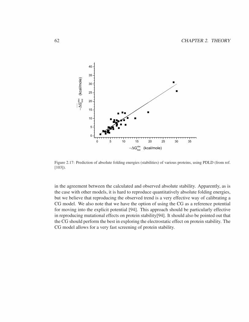
62 CHAPTER 2. THEORY
0 5 10 15 20 25 30 35
0
5
10
15
20
25
30
35
40
Gel
ecfo
ld
(kca
l/mol
e)
Gobsfold
(kcal/mole)
Figure 2.17: Prediction of absolute folding energies (stabilities) of various proteins, using PDLD (from ref.[103]).
in the agreement between the calculated and observed absolute stability. Apparently, as isthe case with other models, it is hard to reproduce quantitatively absolute folding energies,but we believe that reproducing the observed trend is a very effective way of calibrating aCG model. We also note that we have the option of using the CG as a reference potentialfor moving into the explicit potential [94]. This approach should be particularly effectivein reproducing mutational effects on protein stability[94]. It should also be pointed out thatthe CG should perform the best in exploring the electrostatic effect on protein stability. TheCG model allows for a very fast screening of protein stability.

2.3. COARSE-GRAINED MODEL 63
Protein ∆Gobs ∆Gcalcset
Staphylococcal Nuclease 6.2 6.7Staphylococcal Nuclease ∆ + PHS 11.9 7.5
Ribonuclease 10.5 10.7Barstar 5.7 3.1Bc CSP 5 8.7
SS07d 8 10.0Chey 9.5 13.4
FeCyt b562 10.1 10.3Thioredoxin 9 12.0
Apoflavodoxin 4.3 2.5Barnase wt 8.8 11.2
Bnase W94F 8 11.0Bnase W94L 7.5 10.2
Ec DHFR WT 6.1 8.5Ec DHFR W22L 6.2 6.7Ec DHFR W30A 4.0 7.6
bCSP WT 3.5 0.1bCSP F27A 2.7 -0.5bCSP F17A 2 -0.5bCSP F15A 1.2 -0.3
Ribosomal s6 8 6.0λ -Repressor 4.6 7.7
Bs Hpr Phosphotransferase 4 3.7Arc Repressor 4.6 7.7
GDH Domain2 4.9 12.7Ferridoxina - -
Sac7d 7.4 12.4Ubiquitin F45W 7.4 4.7
Interleucine 9.1 15.2R Nase A 9.3 9.2
R Nase T1 7.7 11.9
Table 2.12: Predicted and observed absolute stabilities of a set of proteins, using the CG Model (fromref.[103]). aFerridoxin without the SF4 ligand is considered unstable.
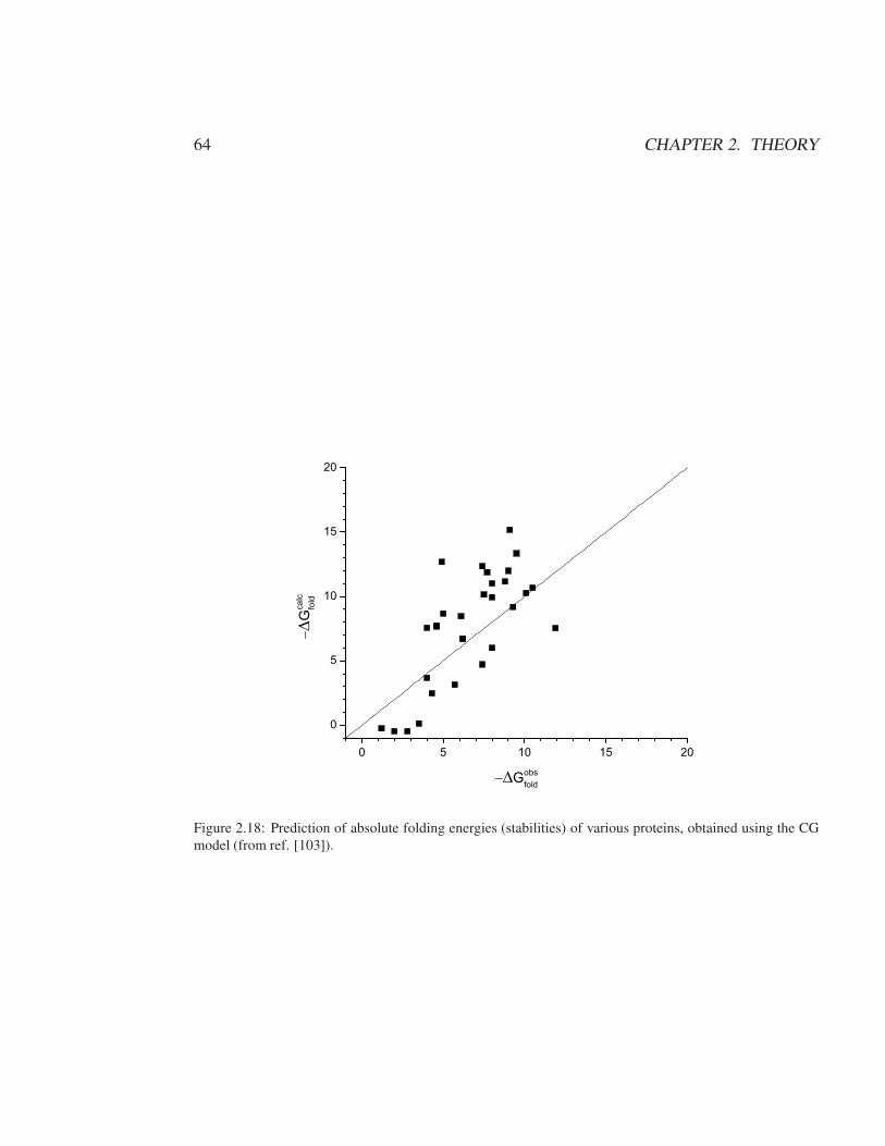
64 CHAPTER 2. THEORY
0 5 10 15 20
0
5
10
15
20
Gca
lcfold
Gobsfold
Figure 2.18: Prediction of absolute folding energies (stabilities) of various proteins, obtained using the CGmodel (from ref. [103]).

2.3. COARSE-GRAINED MODEL 65
2.3.3 Electrolyte and Voltage Effect
The semi-macroscopic strategy used here has been described in our previous electrostaticmodeling [13], which is similar to the approach introduced originally by Klein and Pack[106] but it retains a more microscopic view. The grid spacing is taken here as ∆ andthe volume element τ = ∆3 centered at the ith grid point contains a residual charge qgidetermined by
qgi = q+i + q−i (2.99)
where
qi =α∓Nboxe
( ∓ βφi)
A±=Q±boxe
(∓βφi)
A±(2.100)
where q+i and q−i are, respectively, the positive and negative fractional charges that areassigned to the ith grid point, α∓ is the ion charge of the electrolyte ions in atomic units(namely, ±1 for the 1:1 electrolyte used in our calculations), Nbox box is the total numberof cations/anions in the simulation box, Q±
box box is the total charge of cations/anions inthe simulation system given by Q±
box = α∓Nbox, φi is the electrostatic potential (times unitcharge) at the ith grid point, and β = (kT )−1. A± is a normalization constant. In the initialstep of the calculation Nbox box is obtained as follows for a 1:1 electrolyte:
N±box = nbulkτN
boxgrid (2.101)
where nbulk is number density (number of ions/Angstrom3), which is connected to the molarconcentration (C) by
nbulk =C
1666(2.102)
box Ngridbox is the number of grid points within the simulation box (outside membrane and
protein).Using the normalization condition
∑
q±i on Eq. 2.100, we obtain
qi =α∓Nboxe
∓βφi
∑
i e∓βφi
=Q±boxe
∓βφi
∑
e∓βφi(2.103)
Our normalization treatment, which is different than the common use of the bulk den-sity, helps to obtain a clearer physical picture. However, for a very large simulation systemand at the limit of φ → 0, we obtain:
A± =∑
e∓βφi → Ngridbox (2.104)
The potential times unit charge φ (which is actually potential of mean force) can be ex-pressed as
φi = 332∑
j
qPiǫgpeffrij
+ 332∑
j
qgiǫwatrik
+ V exti (2.105)
where V exti represents the external potential on ith grid point. Here, qPj is the charge of
the jth protein residue (these charges are evaluated by MC procedure described above) and

66 CHAPTER 2. THEORY
qgk is the point charge at the kth grid point (representing the excess net charge of the kthvolume element).
The effect of the regions that are not included in the simulation system was representedby using a partially periodic (quasiperiodic) treatment. That is, we used a periodic boundarycondition with explicit images of the simulation system in the nearest neighbor cells andwith simplified replicas for farther images, where the total charge of the slab at each Zcoordinate is centered on the middle point of the slab (with coordinate (0;0;Z)).
The dielectric ǫgpeff represents charge-charge dielectric for interaction between the pro-tein and the electrolyte grid points. This parameter can be approximated by a large numberbetween 40 and 80 or by the distance dependent function
ǫ = 1 + 60[1− exp(−0.1rij)] (2.106)
In order to model the effect of the external potential, one can consider formally themembrane/ protein/water system as a capacitor. In this case, it is possible to use the well-known macroscopic capacitor model. That is, in principle we can use the well-knownmacroscopic capacitor model , where the external potential induces surface charges (σf ),whose value will be defined below, and creates the corresponding displacement vector D0.In this case, we have
D0 = 4πσf (2.107)
where D0 is not affected by the medium. We also have the relationship
E = D0/ǫ = D0 − 4πP (2.108)
where ǫ is the macroscopic local dielectric constant (which is not equal to the above ǫij), Eis the macroscopic field, and P is the macroscopic polarization.
Our first task is to determine the membrane potential and the electrolytes charges, so wecan evaluate the free energy of the protein charges in the presence of this potential, whichis done by expressing the external potential as
V iext =
∫ zi
z0
D0z/ǫ(z)dz (2.109)
where Z0 is theZ coordinate at the left electrode (in the current work, we define theleft side as the side with smaller value for the Z coordinates and the right side with thelarger Z value). Now, if we consider the potential on the electrolyte grid points or on themembrane grid points, we can define what is considered here as the ideal potential (namely,the potential in regions without the protein) by
V outi = V ideal
i =
(z − zmin) ·D0/ǫwat
z < zig1(zig1 − zmin) ·D0/ǫwat + (z − zig1 ) ·D0/ǫmem
zig1 <= z <= zig2(zig1 − zmin) ·D0/ǫwat + (zig2 − zig1 ) ·D0/ǫmem + (z − zig2 ) ·D0/ǫwat
z > zig2(2.110)

2.3. COARSE-GRAINED MODEL 67
where zig1 is a left boundary of the membrane, zig2 is a right boundary of the membrane,and zmin is the lowest (left-most) Z coordinate of the grid in the system (for this purpose weassume "flat" membrane). Here ǫwat and ǫmem are the dielectric constants of water solutionand the membrane/protein system, respectively. When we deal with the protein chargedgroups, we evaluate the relevant external potential by starting from the closest point, wherewe know the ideal potential of Eq. 2.110. In principle, because the potential is a statefunction, we can choose any path for evaluating the potential at the site of the given sidechain. Our estimate of the potential on the protein sites:
V iext =
V iideali+ VshiftD0(z − zstartpro ) ·
(
1ǫsite(rwat)
− 1ǫideal
)
|rwatcenter − rwat| < 3
V (zstartpro ) +D0·(zcenter−zstartpro )
ǫ(rwatcenter)+ D0·(z−zcenter)
ǫ(rwat)|rwatcenter − rwat| >= 3
(2.111)where the closest distance from the rcenter = (x, y, zcenter) to the closest electrolyte gridpoint is rcenterwat . Here, the distance-dependent dielectric is defined as
ǫ(r) = 34 · e−(x/5)2 + 6 (2.112)
The shift potential, Vshift, is based on the calculation of the grid potential
Vshift = −Vright − Vleft
2(2.113)
For additional details about the model, see Dryga, PNAS, 2012 and molaris demo di-rectory. voltage/barrier/DOCS contains additional information about the model and demoitself. Source code used is from cvs on mykonos and was checked head of trunk on May 3,2012.

68 CHAPTER 2. THEORY

Chapter 3
Specific applications and practical
aspects
3.1 General groups of keywords
The modular implementation of program MOLARIS that we present allows the user to usecommon types of calculations and/or keywords specifications for different types of runs.There exist several groups of keywords that are shared by more than one types of runs.The archaetypical example is the group of keywords md_parm. This group of keywordsis shared by all runs that need MD trajectories to be computed. In this level the user canspecify the characteristics of the run, independently of what kind of run (solvation, EVB,binding...) is being performed. For example, keywords as nsteps, temperature,constraint_pair among others that control typical features of an MD run, can bemodified within this level. Refer to the reference manual for details.
Another group of keywords is the set_opt, that controls all PDLD keywords inPOLARIS runs (from grid spacing to number of iterations and POLARIS radii of the dif-ferent atom types).
3.2 Running the program and updating the amino acid
library
Run the program by typing
$ molaris
When starting the run you will be prompted by the program. The first thing that you shoulddo is to enter the name of the coordinates file, e.g.:
Input the coordinate file name> sub.pdb
After writing this coordinate file name the program will read this file and report any errorsthat it encounters in the file. The program will automatically read the amino acid library
69

70 CHAPTER 3. SPECIFIC APPLICATIONS AND PRACTICAL ASPECTS
file. This library contains all the information needed to describe the topology and chemicalnature of the molecules that are included in this library. Additional new molecules whichare not included in the library are automatically incorporated. Another automatic procedureis the addition of hydrogens to the protein. After successfully updated the amino acidlibrary, the program will then print out the names of the amino acids and other groups thatit finds in the library.
3.3 Using ANALYZE
After the PDB file has been read and the topology file has been created the program willagain give the prompt:
tasks>
Now you can type ANALYZE in order to get information about the system under study.This is done by using the keywords in the reference manual. The keywords allres,restype and resatom give information about the new numbering in the protein. Youcan use these commands to determine the number of the amino acid that has the atoms ofinterest. Also, you can check the topology of particular residues by typing, for example,resbond, restor,... or even modify this topology file by using addbond.
ANALYZE can also be used for performing simple calculations as the distance betweentwo atoms (distatom), or to list the ionizable groups within a sphere, among others.
The last type of information using ANALYZE is the generation of movies and molecularelectrostatic potentials (MEPs) from restart files taken from previous runs. This is done byusing the keywords view_movie and view_pot. As is explained in the manual, everylevel of MOLARIS is exited by the keywords end or exit.
An example of ANALYZE run is given below, where we calculate the electrostatic in-teractions of SER 47 in BPTI with all the residues within 9.0Å from its center. The inputfile looks as follows:
../../pdb/bpti.pdb
analyze
restype SER
electro 1 9.0 47
end
end
The results of the run will look like:
analyze> restype SER
47 SER_047
analyze> electro 1 9.0 47

3.4. USING ENZYMIX 71
Radius = 9.0A
Total charge on residue 47 = 0.000
The coordinates of the center for residue(s): 47
= 9.575 28.800 1.738
residue# residue charge electro distance(A)
-------- ------- ------ ------- -----------
20 ARG 0.000 -0.082 8.233
21 TYR 0.000 -0.712 5.065
30 CYS 0.000 -0.512 8.435
45 PHE 0.000 1.336 6.417
46 LYS 0.000 -11.561 6.293
48 ALA 0.000 -9.198 4.111
49 GLU 0.000 4.351 4.877
50 ASP 0.000 14.014 4.351
51 CYS 0.000 -4.263 6.003
52 MET 0.000 0.251 8.867
53 ARG 0.000 -0.136 8.502
-----------------------------------------------
total electrostatic energy -6.511 (kcal/mol)
A more advanced demo of using ANALYZE is given in the directory an_total.
3.4 Using ENZYMIX
One of the major class of simulation that can be performed by MOLARIS involves theENZYMIXmodule. This module comes from the implementation in the MOLARIS packageof the previous version of program ENZYMIX. For choosing this module the user shouldtype
tasks> enzymix
and then select from the several options in the menu. Essentially there are severalgeneral classes of simulations that can be performed. The simplest one involves regularMD simulation of the protein without a specific function in mind (e.g.trying to obtain arelaxed structure). This option, which is activated by the keyword RELAX makes use to thegeneral force field of ENZYMIX which is an extension of the classical-classical interactionpotential and the consistent force field developer originally by Warshel, Levitt and Lifson[95, 100]. The second option focused on calculations of chemical reactions in enzymes andsolution using the EVB method. Another option is to obtain the free energy of differenttransformations (e.g.charging of ionizable residues) using the FEP approach. Some of themain options of the ENZYMIX module will be described in detail below.
3.4.1 Simple MD relaxation of a macromolecule
The simplest tast of ENZYMIX is to run MD simulations of macromolecule without adress-ing specific functional aspect. An example of a relaxation run is given in the directoryez_relax. The input look like:

72 CHAPTER 3. SPECIFIC APPLICATIONS AND PRACTICAL ASPECTS
../pdb/bpti.pdb keeph #Keeping Good Hydrogens from the PDB
analyze
allres
resatom 33
resatom 57
end
enzymix
relax
md_parm #how to change the default parameters
nsteps 100
temperature 200.0
stepsize 0.0002
constraint_1 30.
constraint_2 60.
langevin_r 18.
water_r 10.
2r 10.
end
end
end
analyze
makepdb #creating a .pdb file with relaxed structure
residue all
file_nm $OUT_DIR/bpti_relax.pdb
end
end
end
The beginning of the output file gives information about the system. Among otherinformation MOLARIS prints the cutoff radii, the number of atoms, bonds, angles, torsionsand improper torsions, as well as the number of residues and electroneutral groups. This isfollowed by the sequence of your system. After which the following information is printed:
Solvent generation: water
Solvent radius : 10.00
There are 10 solvent within a distance of 10.0 Angstroms
of the center: 14.6 21.1 4.1
--------------------------------------------------------------------
Exclusion of protein groups
Center for water and region II : 14.63 21.11 4.14
Radius for region II (dynamics & electro) : 16.00 18.00
total # of protein atoms : 895
# of atoms in region I : 0
# of atoms in region II : 837
# of atoms in region III (dynamics & electro) : 58 25
total # of electroneutral groups : 217
# of groups in region III (dynamics & electro): 13 5
--------------------------------------------------------------------
Langevin dipole generation
the born radius = 18.00
the water radius = 10.00
number of langevin points = 182
The GAP info will be written in:
/tmp/nili/output/gap.out
--------------------------------------------------------------------
Nonbonded pairlist generation
Generated pro-pro nonbond pairlist - interactions: 97346

3.4. USING ENZYMIX 73
Generated pro-wat nonbond pairlist - interactions: 6261
Generated wat-wat nonbond pairlist - interactions: 234
Step cpu time = 1.01 sec ( 0.0 min)
-----------------------------------------------------------------------
Step cpu time = 0.00 sec ( 0.0 min)
Created file (unit= 20):
/tmp/nili/output/rest.scratch
Total charge for the regions I+II (ac or evb included): 0.000
You should always control if these printed parameters, like cutoff radii, the center ofthe system, the total charge of the system are what you expected.
Energies for the system at step 0:
------------------------------------------------------------------------
protein - ebond : 256.34 ethet : 436.22
ephi : 1023.98 eitor : 89.87
evdw : 3340.06 emumu : -809.34
ehb_pp : -109.76
water - ebond : 0.75 ethet : 0.00
evdw : -0.41 emumu : 8.43
ehb_ww : 0.00
pro-wat - evdw : -8.48 emumu : 9.37
ehb_pw : 0.00
long - elong : -3.84
ac - evd_pop : 0.00 emumupop : 0.00
evd_pow : 0.00 emumupow : 0.00
ehb_pop : 0.00
ehb_pow : 0.00
evb - ebond : 0.00 ethet : 0.00 ephi : 0.00
evdw : 0.00 emumu : 0.00 eoff : 0.00
egpshift : 0.00
induce - eind : 0.00 eindw : 0.00
const. - ewatc : 61.70 eproc : 0.00 edist : 0.00
langevin- elgvn : 0.00 evdw_lgv : 115.77 eborn : -3.10
system - epot : 4407.56 ekin : 0.00 etot : 4407.56
The meaning of the different terms is defined in the glossary in the output file and isalso given below:
Glossary for energy terms:
protein - ebond: energy of all bonds of the protein
- ethet: energy of all bond angles of the protein
- ephi : energy of all torsional angles ofthe protein
- eitor: energy of all improper torsional angles of protein
- evdw : van der Waals interaction between region2 atoms
- emumu: Coulombic interaction between region2 atoms
- ehb_pp: H-bond interaction between region2 atoms
water - ebond: energy of all bonds of the water molecules
- ethet: energy of all bond angles of the water molecules
- evdw : van der Waals interaction between water atoms

74 CHAPTER 3. SPECIFIC APPLICATIONS AND PRACTICAL ASPECTS
- emumww: Coulombic interaction between water atoms
long - elong: energy of long range interaction beyond cutoffs in
system+water
poly - evd_pop: van der Waals contribution for region1-region1 atoms and
region1-region2 atoms interaction
- emumupop: Coulombic contribution between region1-region1 atoms and
region1-region2 atoms interaction
- evd_pow: van der Waals contribution between
region1-water atoms interaction
- emumupow: Coulombic interaction between region1-water atoms
- ehb_pop: H-bond interaction between region1-region1 atoms and
region1-region2 atoms
- ehb_pow: H-bond interactio betweenregion1-water atoms
quantum - ebond: energy of all bonds of the EVB atoms
- ethet: energy of all angles of the EVB atoms
- ephi : energy of all torsional angles of the EVB atoms
- evdw : van der Waals interaction between
EVB-EVB atoms and EVB-protein atoms
- emumu: Coulombic contribution for the EVB-EVB
and EVB-protein interaction
- eoff: off diagnal interaction for EVB-EVB atoms
induce - eind: induced energy of atoms in the system
- eindw: induced energy for water atoms in the system
const. - ewatc: constrain energy of water atoms
- eproc: constrain energy for protein atoms
- esetc: constrain energy for specified atoms
langevin- ewatc: energy of the langevin dipoles
- evdw_lgv: van der Waals interaction for langevin dipoles
system - epot: total potential energy of the system
- ekin: total kinetic energy of the system
- etot: total energy of the system
In this example the entries under poly, quantum and induce are all zero as we did nei-ther define quantum nor POLY atoms nor use induced dipoles or forces in the calculation.
After this energy breakdown for the entire system comes the breakdown for the POLYatoms. As we did not define any POLY atoms here most of the numbers are zero and wedo not have to look at this part now.
After this we get information about the temperature. In the beginning of a MD simula-tion the actual temperature can deviate from the target value. But after about 200 steps itshould be very close to the target temperature and should not fluctuate.
In dynamics: Istep= 31 Temp= 217.15 Target= 200.00
In dynamics: Istep= 32 Temp= 216.09 Target= 200.00
In dynamics: Istep= 33 Temp= 215.06 Target= 200.00
In dynamics: Istep= 34 Temp= 214.08 Target= 200.00
In dynamics: Istep= 35 Temp= 213.13 Target= 200.00
In dynamics: Istep= 36 Temp= 212.23 Target= 200.00
In dynamics: Istep= 37 Temp= 211.36 Target= 200.00
In dynamics: Istep= 38 Temp= 210.54 Target= 200.00
In dynamics: Istep= 39 Temp= 209.76 Target= 200.00
In dynamics: Istep= 40 Temp= 209.03 Target= 200.00
The program also prints the rms values for the geometrical changes during the MDsimulation.
rms of all protein heavy atoms atoms for (x_average-x0) = 0.03
rms of all protein heavy atoms atoms for (x_current-x0) = 0.05
This value should be small, for MD simulations at room temperature this rms value isnormally around 1.0 ± 0.5 Å. At the end of the MD simulation an output of the averageenergy over all steps is printed and one where the first 350 steps are interpreted as a relax-

3.4. USING ENZYMIX 75
ation and are not used in the averaging procedure. Note: In this example for the rms of allregion I atoms nan is printed. This is due to the fact that no region I atoms were definedand not an error.
Note: The amount of output generated during an ENZYMIX run is controlled by thelast flag in the file solvent.opt. If you set this flag to 0 you get a short output whereas 1
generates the long output.
3.4.2 EVB calculations
In order to demonstrate the EVB method we will consider the specific case of the catalyticreaction of subtilisin. We describe below the steps involved in the calculations.
Preparing the EVB run
Before we start the actual calculation we have to spend some thoughts upon the mechanismof the enzymatic reaction we wish to analyze and the selection of the EVB atoms. Theenzyme subtilisin catalyzes the cleavage of peptide bonds and the residues directly involvedin this reaction are SER 221, HIS 64, ASP 32 and TYR 276. We will model the reactionby a two step mechanism. The first step is a proton transfer (PT) from SER 221 to HIS64 which is followed by the nucleophilic attack (NA) of the deprotonated SER 221 on thecarbonylic carbon of TYR 276.
As pointed out in section 2.1.7 all those atoms that undergo a change in their bondingpattern or their charge distribution have to be treated as EVB atoms. With this in mind weend up with the three resonance forms shown in Figure 3.1.
Our first task is to define the EVB atoms in the overall list of the atoms of the simulatedsystem. Since the study of enzyme catalysis involves comparison of the reaction in enzymeand in solution we will have to study the reaction in both systems. In the case of theenzyme we start by running an analysis of the enzyme region 1. The subtilisin demo isprovided in the directory ez_EVB:
pdb/sub.pdb
# check the numbering of the evb atoms
analyze
resatom 32
resatom 64
resatom 221
resatom 276
resatom 277
end
The output of this run allows us to find the numbers of the relevant protein atoms and toassign to them the corresponding EVB atom types (Fig. 3.1). The result of this assigmentis summarized in Table 3.12 and the users are advised to construct a similar table for theirspecific protein. At this point it is useful to consider the correspondance between Table3.12 and Fig .3.1.

76 CHAPTER 3. SPECIFIC APPLICATIONS AND PRACTICAL ASPECTS
Figure 3.1: The three EVB resonance forms for modeling the enzymatic reaction of subtilisin. EVB atomsare numbered in bold face type (for the reaction in the enzyme - a similar assignment of EVB atoms for thereaction in solution is required). The ASP 32 shown on the right is not part of the EVB resonance forms,while Nα and NH of the neighboring C-terminal GLY 277 have been included as EVB atoms due to anincreased stability encountered during the simulation.
The first resonance form corresponds to the reactants, the second to the product of thePT step and the third shows the resulting structure after the NA step. The EVB region iscomprised of the OH group of SER 221, the imidazole ring of HIS 64, the carbonyl groupof TYR276 and the Nα and HN of the C-terminal GLY 277. Note: When defining the EVBatoms you should always include all atoms forming an electroneutral group. Taking onlypart of the atoms of an electroneutral group can lead to strange results, when calculatingthe overall charge of the complete system.
For the EVB run you need, of course, the proper EVB parameters. Sometime the pa-rameters may already be included in the default evb.lib. In other cases you will have torefine the proper parameters, see section 3.4.8. At any rate, in the present demo we provideyou with the proper evb.lib. Also note that for the protein run we have to define the ion-ization state of certain amino acid residues. Remember that the electrostatics are crucial indetermining the reaction profile and if they are treated sloppily then the program will fail
to yield any valuable information. For subtilisin it is known that ASP 32 is in its ionizedform, which must be reflected in the simulation. For other systems you have to make acase by case decision, but sometimes there are experimental results which give you a hintabout the ionization state.
After verifying that we assigned correctly the EVB atoms we can input the informationfor the EVB run. First, we start with a short relaxation run to ensure that the simulationstarts from equilibrated configuration:
# A long relaxation run using EVB force field

3.4. USING ENZYMIX 77
pdb/sub.pdb
enzymix
pre_enz
ionres 32 # ionize the ASP32 residue
end
# define atoms of the EVB region and
# bonding pattern of the three
# resonance forms
evb
evb_state 3 1.0 0.0 0.0 1
evb_atm 889 0.0350 C+ 0.1640 C+ 0.1640 C+
evb_atm 890 0.0150 N+ -0.1610 N+ -0.1610 N+
evb_atm 891 0.1870 H0 0.1870 H0 0.1870 H0
evb_atm 892 0.1100 C+ 0.5450 C+ 0.5450 C+
evb_atm 893 0.0750 H0 0.0750 H0 0.0750 H0
evb_atm 894 -0.5200 N+ -0.1610 N+ -0.1610 N+
evb_atm 895 0.0280 C+ 0.0960 C+ 0.0960 C+
evb_atm 896 0.0700 H0 0.0680 H0 0.0680 H0
evb_atm 3026 -0.4270 O0 -1.0000 O- -0.2000 O0
evb_atm 3027 0.4270 H0 0.1870 H0 0.1870 H0
evb_atm 3854 0.3920 C+ 0.3920 C+ 0.2000 C0
evb_atm 3855 -0.3920 O0 -0.3920 O0 -1.0000 O-
evb_atm 3837 -0.0970 C0 -0.0970 C0 -0.0970 C0
evb_atm 3838 0.0970 H0 0.0970 H0 0.0970 H0
evb_atm 3856 -0.4000 N+ -0.4000 N+ -0.4000 N+
evb_atm 3857 0.4000 H0 0.4000 H0 0.4000 H0
evb_bnd 0 889 895
evb_bnd 0 889 890
evb_bnd 0 890 891
evb_bnd 0 890 892
evb_bnd 0 892 893
evb_bnd 0 892 894
evb_bnd 0 894 895
evb_bnd 0 895 896
evb_bnd 1 3026 3027
evb_bnd 2 894 3027
evb_bnd 3 894 3027
evb_bnd 3 3026 3854
evb_bnd 0 3854 3855
evb_bnd 0 3838 3837
evb_bnd 0 3837 3854
evb_bnd 0 3854 3856
evb_bnd 0 3856 3857
gas_dg 1 0.0
gas_dg 2 115.0
gas_dg 3 50.0
evb_parm
ifglag_r4 0
end
rest_out evb_sub-rx.res # store the relaxed structure
# into a restart file
md_parm
temperature 300
ss 0.0001 # using a small time-step
nsteps 30000
region2a_r 16
water_r 16
langevin_r 18
constraint_pair 894 3026 3.0 3.0
constraint_pair 3026 3854 3.0 3.0
constraint_post 3026 3.0 3.0 3.0 21.4 27.0 20.6
end
end
end
After the relaxation we are ready to prepare the input file for the actual simulation of

78 CHAPTER 3. SPECIFIC APPLICATIONS AND PRACTICAL ASPECTS
Table 3.12: EVB atom Numbers, Types and Charges for the Catalytic Reaction of Subtilisin in Protein andWater
Resonance Form I Resonance Form II Resonance Form IIIWater # Protein # Atom type Charge Atom type Charge Atom type Charge
8 889 C+ +0.035 C+ +0.164 C+ +0.1649 890 N+ +0.015 N+ -0.161 N+ -0.161
10 891 H0 +0.187 H0 +0.187 H0 +0.18711 892 C+ +0.110 C+ +0.545 C+ +0.54512 893 H0 +0.075 H0 +0.075 H0 +0.07513 894 N+ -0.520 N+ -0.161 N+ -0.16114 895 C+ +0.028 C+ +0.096 C+ +0.09615 896 H0 +0.070 H0 +0.068 H0 +0.06825 3026 O0 -0.427 O- -1.000 O0 -0.20026 3027 H0 +0.427 H0 +0.187 H0 +0.18731 3837 C0 -0.097 C0 -0.097 C0 -0.09732 3838 H0 0.097 H0 0.097 H0 0.09748 3854 C+ +0.392 C+ +0.392 C0 +0.20049 3855 O0 -0.392 O0 -0.392 O- -1.00050 3856 N+ -0.400 N+ -0.400 N+ -0.40051 3857 H0 0.400 H0 0.400 H0 0.400
the PT step in the protein. The input file is very similar to the input file of the relaxationrun with a few changes: (i) we need to read in previously stored relaxed structure, (ii) givenumber of mapping steps in the free energy perturbation (FEP) procedure (here we chose11 steps goin from step 1 to step 2), and (iii) set the temperature to room temperature andincrease the time step.
evb> rest_in $OUT_DIR/evb_sub-rx.res
evb> map_pf 11 1 2
md_parm> nsteps 20000
md_parm> ss 0.001
As is clear from section 2.1.8 we should also define the off-diagonal matrix elements.Different options are available for the analytical form of Hij . Here we are not using it.
If you do not know what value to take, you can set the Hij to zero, which is perfectlylegal as long as you only discuss the differences in the free energies and no absolute values.As a rough guess you can also use Hij of similar examples from literature. Rigorously, thevalue of the parameters for Hij should be refined either by fitting the gas phase potentialsurface to ab initio quantum mechanical calculations or by fitting the barrier of the reactionin solution to its observed values.
Complete input files evb_subwat_12.inp and evb_sub_12.inp for simulationof the PT step of the subtilisin reaction both in water and enzyme, respectively, can befound in ez_EVB directory.
3.4.3 Simulating the PT reaction of Subtilisin
After finishing the preparation step we submit the simulation runs for the reactions inthe enzyme and in water. This can be done by running the command run_demo in thesubtilisin demo directory ez_EVB. When the runs are finished we can examine the outputfiles. A typical output includes a list of the EVB parameters. For example the nonbondedparameters:
Nonbonded Parameters for evb-evb

3.4. USING ENZYMIX 79
The most important results are those given in the breakdown of the EVB energies:
EVB Electrostatic Energies Breakdown
State Total Coulombic/pro Coulombic/wat Indu/evb Indu/pro Indu/wat Intra
------- ------- ------------- ------------- -------- -------- -------- -------
1(1.00) -84.89 -48.67 0.77 0.00 0.00 0.00 -36.99
2(0.00) -208.21 -74.13 1.97 0.00 0.00 0.00 -136.05
3(0.00) -226.57 -98.06 1.76 0.00 0.00 0.00 -130.27
EVB Total Energies -- Hamiltonian Breakdown
State Total Egas Bond Angle Torsion Eqmu Eind Vdw Bulk
------- ------ ------ ----- ------- ------- ------ ------ ------- ------
1(1.00) -24.1 0.0 40.0 20.4 23.7 -84.9 0.0 34.4 -57.8
2(0.00) 192.6 115.0 117.1 54.4 55.5 -208.2 0.0 117.9 -59.1
3(0.00) 195.5 50.0 167.8 91.5 75.8 -226.6 0.0 94.4 -57.4
VDW Energy Breakdown
State Total Enviroment ( protein, water ) Intra
------- ------- ---------- ------- ------- -------
1 34.4 16.3 ( 19.1 -2.8 ) 18.1
2 117.9 20.6 ( 23.4 -2.8 ) 97.3
3 94.4 20.8 ( 23.6 -2.8 ) 73.6
BULK Energy Breakdown
State Total langevin born
------- ------- ---------- --------
1 -57.8 0.0 -57.8
2 -59.1 0.0 -59.1
3 -57.4 0.0 -57.4
EVB energy matrix
1 2 3
1 -24.13
2 0.00 192.59
3 0.00 0.00 195.53
Hamiltonian Eigenvectors and Eigenvalues
1 2 3
-24.13 192.59 195.53
1 0.00 1.00 0.00
2 1.00 0.00 0.00
3 0.00 0.00 1.00
3.4.4 Interpreting the Results of an Enzymix Run
Each ENZYMIX run generates a set of so called energy gap files, one for each λ value. Atevery tenth step during the MD simulation all relevant information about the energy ofyour system is written to these files. In the following mapping procedure this informationis read from these files and processed by the mapping program. The mapping commandfile evb_subwat-map.inp for our example of the water reaction of the proton transferstep in subtilisin is given in the demo directory ez_EVB. The input looks like:
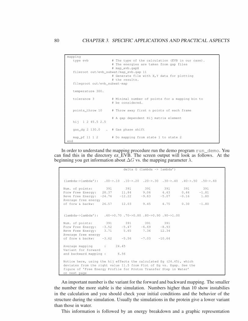
80 CHAPTER 3. SPECIFIC APPLICATIONS AND PRACTICAL ASPECTS
mapping
type evb # The type of the calculation (EVB in our case).
# The energies are taken from gap files
# map_evb.gapX
fileroot out/evb_subwat/map_evb.gap 11
# Generate file with X,Y data for plotting
# the results.
filegroot out/evb_subwat-map
temperature 300.
tolerance 3 # Minimal number of points for a mapping bin to
# be considered.
points_throw 10 # Throw away first n points of each frame
# A gap dependent Hij matrix element
hij 1 2 45.5 2.5
gas_dg 2 130.0 . # Gas phase shift
map_pf 11 1 2 # Do mapping from state 1 to state 2
end
In order to understand the mapping procedure run the demo program run_demo. Youcan find this in the directory ez_EVB. The screen output will look as follows. At thebeginning you get information about ∆G vs. the mapping parameter λ.
delta G (lambda -> lambda’)
(lambda->lambda’): .00->.10 .10->.20 .20->.30 .30->.40 .40->.50 .50->.60
Num. of points: 391 391 391 391 391 391
Forw Free Energy: 28.37 11.84 9.06 4.43 0.44 -1.81
Reve Free Energy: -24.76 -12.22 -9.83 -5.07 -0.16 1.80
Average free energy
of forw & backw: 26.57 12.03 9.45 4.75 0.30 -1.80
(lambda->lambda’): .60->0.70 .70->0.80 .80->0.90 .90->1.00
Num. of points: 391 391 391 391
Forw Free Energy: -3.52 -5.47 -6.69 -8.93
Reve Free Energy: 3.71 5.65 7.36 12.34
Average free energy
of forw & backw: -3.62 -5.56 -7.03 -10.64
Average mapping : 24.45
Variant for forward
and backward mapping : 6.56
Notice here, using the hij effects the calculated Eg (24.45), which
deviates from the right value 11.5 from Plot of Eg vs. Egap. See the
figure of ’Free Energy Profile for Proton Transfer Step in Water’
on next page
An important number is the variant for the forward and backward mapping. The smallerthe number the more stable is the simulation. Numbers higher than 10 show instabiliesin the calculation and you should check your initial conditions and the behavior of thestructure during the simulation. Usually the simulations in the protein give a lower variantthan those in water.
This information is followed by an energy breakdown and a graphic representation

3.4. USING ENZYMIX 81
of the ∆G vs. λ curve. Normally the contributions from bond, angle and torsion termsare small and the dominating contribution is the electrostatic energy, as is the case in thisexample. The output also provides the result from the linear response approximation,but for EVB calculations the LRA result should be ignored. At the end you find themost important output. The ground state free energy versus the energy gap and the freeenergy surfaces for the two EVB resonance forms. From the ground state free energysurface we get an activation free energy of 14.3 kcal/mol and a reaction free energy of11.5 kcal/mol. The raw data used for these two plots can also be found in the output filedemo_output/evb_subwat_12/evb_subwat-map.log.
Plot of delta G vs. lambda
53.09 | *50.97 | * *48.85 |
46.72 | * *44.60 |
42.47 |
40.35 | *38.23 | *36.10 |
33.98 | *31.86 |
29.73 |
27.61 |
25.48 | *23.36 | *21.24 |
19.11 |
16.99 |
14.87 |
12.74 |
10.62 |
8.49 |
6.37 |
4.25 |
2.12 |
0.00 |*|-------------------------------------------------------------
0.0 0.1 0.2 0.3 0.4 0.5 0.6 0.7 0.8 0.9 1.0
Examine how the plot of the energy profile, Eg vs. Egap (ε2−ε1), changes upon chang-ing ∆α. You will find that the free energy of the reaction ∆Gij (the difference between thelast and first point of the profile) depends almost linearly on ∆α. This suggests a simpleway of determining ∆α. That is, ∆α is a constant which will have the same effect if itis used in ENZYMIX through Eq. (2.26) or in the mapping program. Thus, we may takethe raw data of an ENZYMIX run for the given reference reaction in water and plot themwith a first guess of ∆α. Next we change ∆α until the calculated ∆Gij reproduces thecorresponding observed ∆Gij . This ∆α will then be kept unchanged in the study of thesame reaction in the enzyme active site.
There is actually a more stringent way to determine the value of this parameter, whichshould be used to check your result for ∆α see refs [1, 107]). The gas phase shift is givenby the following thermodynamic cycle.

82 CHAPTER 3. SPECIFIC APPLICATIONS AND PRACTICAL ASPECTS
-350 -300 -250 -200 -150 -100 -50 0 50 100
Egap
0
2.5
5
7.5
10
12.5
15E
g
Free Energy Profile for Proton Transfer Step in Water
Plot of Eg vs. Egap
∆α
Roo
(g)
Roo
(aq) Poo
(aq)
Poo
(g)
∆Grxnaq
Σ∆Gsol(R) Σ∆Gsol(P)
Figure 3.2: Thermodynamic cycle to determine the gas phase shift ∆α

3.4. USING ENZYMIX 83
Here ROO and POO denote the reactant and product state with the relevant fragments atinfinite distance. Thus,
∆α = ∆Gsol(R) + ∆Gaqrxn −∆Gsol(P ) (3.1)
∆α = ∆∆Gsol +∆Gaqrxn
with ∆Grxn being the experimental value of the reaction free energy. The solvation freeenergies ∆Gsol(R) and ∆Gsol(P) are either experimentally known or you can calculate themwith POLARIS or ENZYMIX. In this way you can check your ∆α against the theoreticalvalue. This is something you should always do before starting long ENZYMIX calculations.If you find a huge difference between these two numbers you should carefully check yoursimulation setup. You might, however, observe small differences between the theoreticaland actually used ∆α. This can have two reasons:(i) Because your reactants and/or product fragments are not at infinite distance, they arestill interacting and you add an extra energy term.(ii) Because your off-diagonal element Hij is not zero at the reactant and product state. Youcan estimate this effect using the expansion:
Eg = min(ε1 − ε2)−H2
12
|ε1 − ε2|+
H412
|ε1 − ε2|
3
· · · (3.2)
Note: This expansion can only be applied if H212/|ε1 − ε2| < 1.
Calculate the value of Eg by inserting the average simulation value of Hij and ε1 − ε2 atthe product state and do the same for the reactants. The difference between the reactant andproduct energy gives you the correction for your ∆α.
The results of the EVB calculations depend on the off-diagonal element of Equation(2.28). Sometimes your initial estimate of Hij might be inadequate and you may use themapping procedure to obtain a better estimate. That is, you may run first the mappingprogram with the initial estimate of Hij . Now compare the barrier of the calculated profileof the reference reaction in water to the corresponding observed barrier. If the barrier istoo high use the factor in line 18 and increase Hij until you reproduce the observed barrierfor the reference reaction. This Hij will be used without change in studying the givenenzymatic reaction. The next chapter demonstrates how to refine the EVB parameters.
To simulate the catalytic effect of subtilisin in the proton transfer step you also haveto calculate the reaction in the protein. The final mapping result for the protein reaction isshown in figure 3.3.
The activation free energy for the PT in the protein is around 15.08 kcal/mol and thereaction free energy around 13.8 kcal/mol. Comparing these numbers with those from thewater reaction (∆g‡=14.3 kcal/mol and ∆G=11.5 kcal/mol) we get no catalytic effect fromthe enzyme. But this result is actually not so bad, as the major contribution to catalysisshould come from the second step, the SN2 reaction.

84 CHAPTER 3. SPECIFIC APPLICATIONS AND PRACTICAL ASPECTS
-250 -200 -150 -100 -50 0 50 100
Egap
0
2.5
5
7.5
10
12.5
15
17.5
Eg
Free Energy Profile for Proton Transfer Step in Protein
Plot of Eg vs. Egap
Figure 3.3: The final mapping obtained for the raction in the protein.
3.4.5 Simulating the SN2 reaction of Subtilisin
In the SN2 reaction of subtilisin the negatively charged oxygen attacks the carbonylic car-bon of TYR 276 and forms a tetrahedral intermediate. The computational procedure isanalogous to the treatment of PT step. We start by relaxation at low temperature, then runactual simulation of the reaction at room temperature and then run mapping to obtain freeenergy profile. All input files needed to run SN2 reaction can be found in ez_EVB demodirectory. Calculated free energy profiles are shown in figures 3.4 and 3.5. By comparisonof activation barriers of the PT and the SN2 reactions in water solution and in the proteinwe conclude that overall catalytic effect of subtilisin is about 8 kcal/mol.

3.4. USING ENZYMIX 85
-400 -300 -200 -100 0 100 200 300
Egap
-5
-2.5
0
2.5
5
7.5
10
12.5
15
17.5
20
Eg
Free Energy Profile for Nucleophilic Attack in Water
Plot of Eg vs. Egap
Figure 3.4: Free energy profile for the reaction in solution.
-200 -100 0 100 200 300
Egap
-2.5
0
2.5
5
7.5
10
12.5
Eg
Free Energy Profile for Nucleophilic Attack in Protein
Plot of Eg vs. Egap
Figure 3.5: Free energy profile for the reaction in the enzyme.

86 CHAPTER 3. SPECIFIC APPLICATIONS AND PRACTICAL ASPECTS
3.4.6 Ground state EVB calculations
When running ground state calculations the bond orders are evaluated at each point duringthe simulation, by diagonalizing the Hamiltonian in Eq. 2.28. Thus we have a way ofrunning direct dynamics on the actual ground state potential energy surface of the systeminstaed of on the mapping potential, as we do in regular EVB/FEP/US calculations. In mostof the cases of interest, barriers for reaction are too high to be surmounted by regular MDcalculations on the ground state potential energy surface. This is the reason why it is morecommon to use EVB/FEP/US for perfoming reactivity studies in enzymes and in solution.However, in some cases it can be of interest to run trajectories on the actual ground statesurface in order to evaluate several properties, such transmission factors in transition statetheory or the study of the fluctuations of the environment in a reactive system.
The way of running ground state calculations is similar to the regular EVB/FEP/US inthe way the EVB region is determined.
3.4.7 Adiabatic charging (AC) and other FEP calculations
The FEP calculations of section 2.1.2 are convinient to be implemented in ENZYMIX. Inparticul ar the program emphasizes calculations of electrostaticfree energy that are referedto as adiabatic charging (AC) calculations [7]. Simple example of such calculations can beobtained by charging a Cl ion. This is done in the demo directory ez_AC. The programconsider auto matically the charging of the atoms in region I and change their charges fromthe initial to final charge states. The input looks like:
../pdb/cl.pdb
enzymix # enter the package enzymix
ac # perfom an adiabatic charging calculation, in order
# to evaluate solvation free energy of Cl.
rest_in cl.res # read a restart file which contains a
# relaxed system of Cl- in water
reg1_atm 1 to 1 # choose Cl as region I atom, whose AC
# is going to be calculated.
ab_crg 1 -1.0 0.0 # assign the cherges of the atom 1 to change from
# -1 to zero (in states A and B respectivly.
map_lambda 1.0 # The AC mapping parameter, states that we start
# from 100
map_pf 11 1 2 # the number of frames to map the free energy for
# the process of changing the system from state
# 1 to state 2
md_parm # specifying a few parameters for the MD (the
# rest will be the default ones.
temperature 300 # temperature is 300K
nsteps 100 # number of steps 100
stepsize 0.001 # step size is 0.001 ps
end
end
end
The output looks like:
put output from AW choice after running
After this we need to run the mapping program.The program can be used in more chalenging calculations such as the free energy of
charges in prote ins. Excellent examples are microscopic calculations of pKas in proteins

3.4. USING ENZYMIX 87
[7], which use the thermodynamic cycle described in section 2.2.5 and the AC processdepicted in Fig. 2.1. A typical example is given in the demo directory ez_AC.
3.4.8 Refinement of the EVB parameters
Refining EVB parameters in the gas phase using MOLARIS:
First you need to have the gas phase experiments or gas phase ab initio scans at fixeddistances to obtain the desired Hij . As an example we consider here the reaction of theproton transfer from H3O+ to H2O. For this reaction type we need to calculate the gasphase ab initio scans between two oxygens, which are held at fixed distances (e.g. 2.8, 3.0,3.2 Å and so on). A sample input file is provided below:
h3o_h2o.pdb #PDB file with H3O+ to H2O (note: the angles between O-H-O
#equals 180 degree so that the proton slowly moves
#on a straight one dimensional line
enzymix #enter the enzymix level
evb #enter the evb level
evb_state 2 1.0 0.0 #describing the evb states
evb_atm 1 -0.65 O+ -0.80 O0 #describing the avb atom types
evb_atm 2 0.55 H+ 0.40 H0
evb_atm 3 0.55 H+ 0.40 H0
evb_atm 4 0.55 H+ 0.55 H+
evb_atm 5 -0.80 O0 -0.65 O+
evb_atm 6 0.40 H0 0.55 H+
evb_atm 7 0.40 H0 0.55 H+
evb_bnd 0 1 2 #describing the evb bonds
evb_bnd 0 1 3
evb_bnd 1 1 4
evb_bnd 0 5 6
evb_bnd 0 5 7
evb_bnd 2 5 4
bond_rigid_map 1 4 5 1 2 0.0 0.0 0.0 #bond rigid map (see below)
md_parm #by default these calculations run in the gas phase
nsteps 0
end #exit md_parm level
end #exit evb level
end #exit enzymix level
end #exit MOLARIS
The bond_rigid_map keyword used above can be utilized in various ways:
• BOND_RIGID_MAP (inside the level enzymix/.../evb)
USAGE: bond_rigid_map 2 5 7 1 2 0.0 10.0 2.0 ORbond_rigid_map 2 5 7 1 2 0.0 10.0 2.0 xyz.pdb 15 ORbond_rigid_map 2 5 7 1 2 0.0 10.0 30.0 2.0

88 CHAPTER 3. SPECIFIC APPLICATIONS AND PRACTICAL ASPECTS
specifying the 3 atoms, 2 evb states, gas phase energy shifts and Hij for rigid bondenergy mapping for reactions like: N- - -H- - -O, were H is rigidly moved from bond N- --H to H- - -O while the positions of all other EVB atoms, except H, are fixed (e.g., for thebond formed by evb atoms 2 and 5 in evb state 1 to the bond formed by evb atoms 5 and 7 inevb state 2; the gas phase shift for state 1 is 0.0, for state 2 is 10.0 and the coupling constantHij between state 1 and 2 is 2.0). The R(NH) vs. E_state1, E_state2 and Eground_state arewritten to the file: evb_rigid_map.dat. In the second example the user specifies a PDB fileroot name and how many file there are, the positions of all evb atoms at each mapping pointare read from each PDB file. The file name should be the root file name appended with a2-digit number (e.g., the PDB files are xyz.pdb02, ..., xyz.pdb015) in the 2nd example, itmay not be RIGID mapping, since the positions of all evb atoms may have changed at eachmapping point in the PDB files. In the third example, the last 2 parameters are A and mufor Hij by the formula:
Hij = A ∗ exp(−mu ∗ r)
where A = 30.0 and mu = 2.0.
The output folder contains the evb_rigid_map.dat file with data and the EVB parametersused in the current EVB run. You may plot the above data to get a mapping-curve (Eg(r)).For example:
R(O+...H+) Eevb1,total Eevb2,total Eevb,ground0.60 529.52 847.88 529.520.62 495.21 821.28 495.210.64 464.34 796.31 464.340.66 436.63 772.88 436.630.68 411.81 750.89 411.810.70 389.63 730.26 389.630.72 369.86 710.92 369.860.74 352.29 692.81 352.290.76 336.74 675.85 336.74

3.4. USING ENZYMIX 89
The EVB parameters are from your evb.lib, but you may change the gas phase energyshifts, Hij and charges and rerun to produce a desired mapping-curve fit. An example ofE1, E2 and Eground are shown in figure 3.6. Here, for bond_rigid_map, we use:
Distance for O+ ... O+ (fixed.pdb) 3.0
The evb atom types in evb state1 O+—H+- - -O0The evb atom types in evb state2 O0- - -H+—O+The equilibrium bond length 1.10 1.10Morse bond parameter D 97.21 97.21
VDW A, Beta dor atom1 evb state1 35.00 2.50VDW A, Beta for atom2 evb state1 50.00 2.50VDW A, Beta for atom3 evb state1 53.00 2.50
VDW A, Beta for atom1 evb state2 53.00 2.50VDW A, Beta for atom2 evb state2 50.00 2.50VDW A, Beta for atom3 evb state2 35.00 2.50
Gas phase energy shifts for states 0.00 0.00Coupling constant Hij 0.00
Charges for 3 atoms in evb state1 -0.65 0.55 -0.80Charges for 3 atoms in evb state2 -0.80 0.55 -0.65
Total net charge of all evb state1 1.00Total net charge of all evb state2 1.00
Refining EVB parameters in the gas phase using Mathematica
The description of this program can be found below (script written for Math-ematica) and online at the webpage http://futura.usc.edu/programs/ (file: Refin-ing_EVB_parameters.nb).The Mathematica program is written for the proton transfer reaction O’-H + O" → O’ +H-O". The variables r1 and r2 in the program define the distances between the O’-H inthe bonded state and the O’ to O" distance respectively. The Morse potential function isdefined by
Morse(r_) = 60.0 ∗ (1.0− exp(−1.75 ∗ (r − 1.1)))2
The charges for the reaction and all EVB parameters should be taken from the EVB library.Here we use artificial charges just for demonstration purposes, i.e 0.40 and -0.80 for hy-drogen (qH) and oxygen charges (qO) respectively. The gas phase shifts Egas1 and Egas2should be fitted to the experimental data. For this symmetric reaction Egas1 and Egas2

90 CHAPTER 3. SPECIFIC APPLICATIONS AND PRACTICAL ASPECTS
Figure 3.6: Sample plot of the one dimensional ground state energy Eg and diabatic states E1 and E2 as afunction of the O+ – H+ distance with fixed O+ – O0 distance at 3.0 Å. For this symmetrical reaction the gasphase shift equals zero. Further modification of the EVB parameters will bring the diabatic energies to thesame level.
equal zero. The diabatic energies E1 and E2 are
E1(r1_, r2_) =Morse(r1) + 0.1 ∗ exp(−3.0 ∗ (r2− 2.6))
+ 150.0 ∗ exp(−1.5 ∗ (r2− r1))
+ 332 ∗ qH ∗ qO/r1 + 332 ∗ qO ∗ qO/r2 + Egas1
E2(r1_, r2_) =Morse(r2− r1) + 0.1 ∗ exp(−3.0 ∗ (r2− 2.6))
+ 150.0 ∗ exp(−1.5 ∗ r1)
+ 332 ∗ qH ∗ qO/(r2− r1) + 332 ∗ qO ∗ qO/r2 + Egas2
where the first term is the Morse potential function, the second term is the repulsionenergy between two oxygens; the third term is the repulsion energy between the oxygen andthe hydrogen atoms when they are not bonded; the fourth and fifth term are the electrostaticinteractions between atoms; the last term is the gas phase shift.
The gap-dependent Hij with parameters (which should be changed for specific runs)are:
c1 = 50; c2=50; b=0.1; a =12
H(egap_) =a ∗ (1.0/(1.0 + exp(−b ∗ (egap− c1)))
+ 1.0/(1.0 + exp(−b ∗ (egap− c1)))− 1)
Hgap2(r1_, r2_) = H(E2(r1, r2)− E1(r1, r2))2 (3.3)
The ground state energy:
Eg(r1_, r2_) =0.5 ∗ (E1(r1, r2) + E2(r1, r2)
−√
(E1(r1, r2)− E2(r1, r2))2 + 4.0 ∗ 100.0)

3.4. USING ENZYMIX 91
The plot of the one dimensional ground state energy Eg and diabatic states E1 and E2as a function of the O-H distance (r1) with fixed O-O distance (r2) at 3.0 Å is shown infigure 3.7. The two dimensional plot of the ground state energy Eg as a function of the
Figure 3.7: Plot[E1(r1,3.0),E2(r1,3.0),Eg(r1,3.0)], [r1, 0.0, 3.0], Plot range → [-50:50].
distances r1 and r2 is shown in figure 3.8; For a symmetric representation we redefine the
Figure 3.8: Contourplot[Eg(r1,r2),(r2,3.0,6.0),(r1,0.8,4.0), Contour labels → True, Contours → 20, Axisstyle→ Directive (blue,16)]
r1 and r2 distances: r1 is the distance between the O’-H and r2 is the distance betweenH-O". Here we redefine the diabatic energies E11 and E22, the off-diagonal element Hij
and the ground state energy Eg:
E11(r1_, r2_) = E1(r1, r1 + r2);E22(r1_, r2_) = E2(r1, r1 + r2)
Hgap2(r1_, r2_) = H(E22(r1, r2)− E11(r1, r2))2
Eg(r1_, r2_) =0.5 ∗ (E11(r1, r2) + E22(r1, r2)
−√
(E11(r1, r2)−E22(r1, r2))2 + 4.0 ∗Hgap2(r1, r2))

92 CHAPTER 3. SPECIFIC APPLICATIONS AND PRACTICAL ASPECTS
The two dimensional plot of the ground state energy Eg as a function of the new r1 and r2distances is shown in figure 3.9:
Figure 3.9: Contourplot[Eg(r1,r2),(r2,0.8,4.0),(r1,0.8,4.0), Contour labels → True, Contours → 20, Axisstyle→ Directive (blue,16)]

3.4. USING ENZYMIX 93
3.4.9 QM/MM calculations
Molaris 9.11 QM/MM 2.1.10 utilities have been redesigned and upgraded for free energycalculations and related tasks in the condensed phase. Since QM/MM calculations, es-pecially those involving the ab initio QM, are computationally expensive all developmentis made to facilitate one of methods for improving the sampling efficiency. Molaris9.11main develpment has been focused on utilizing the idea of the reference potential, whichis also called the Paradynamics approach. In this view all QM/MM calculations are runon AC/MM (AC level) or EVB/MM (EVB level) by substituting the QM part by the de-sired QM potential. On both AC or EVB(and related) level you are required to specifythe region_1 atoms or EVB atoms. Those will be your QM region. In this division makesure not to divide the electroneutral groups, include them either to QM or MM region.mopacRS.pdb keepallh
ez
adiab_tem
evb_state 2 1.0 0.0
rest_out relax_pm3.res
read_evb evb_ref_updated.dat
evb_parm
itflag_r4 0
d
#debug_qm #to see more of QM print out
md_parm
nbupdate 2
log_write_fq 5000
#QM/MM can also be run in vacuum or for COSMO (requires to modify qm_script_qchem4.py)
# gp 1
constraint_ang 1 2 6 15.0 180.
nsteps 20000
#it’s always good to check numerical and analytical derivatives for consistency
# check_all_f
temp 273
ss 0.0003
# no_bulk #E_bulk doesn’t have contributions to dE/dX
qmmm #activates QM/MM
#to sample on the QM/MM potential QM program must be called each step
#you can call each n-th step ONLY at evb(adiab_tem) levels with evb_trajec on
qmmm_interval 1 #+#
script /tmp/FEP_PDMTD/1/qm.csh #script name
qmmm_in /tmp/FEP_PDMTD/1/QProg2/mol.in #input for qm_script_qchem4.py
qmmm_out /tmp/FEP_PDMTD/1/QProg2/d.o #output read by MOLARIS
#This keyword is for MOLARIS/QChem3.2(4) interface It uses electric field on MM atoms
#See QChem manual for their flexible QM/MM interface made for CHARMM
#it’s compatible with MOLARIS9.11 (Advanced, Optional)
# use_qm_efield
#This keyword is required
qmmm_noaver
#Use this keyword for the link atom charge redistribution, note that it makes num and
#analyt derivatives on the host atoms slightly off
red_lk_crg
#You can run evb(adiab_tem) trajectory and calculate energy for each configuration
#with the frequency specified by qmmm_interval
# evb_trajec
#This keyword is for semiempirical QCFFPI and MOPAC2009 interfaces
# cl_elec
end
Currently QM/MM operates with the following external programs as of JAN’12: Gaus-sian03, QChem 3.2(4.0), QCFFPI, MOLARIS, MOPAC2009. The interface is quite flexi-ble. MOLARIS creates mol.in file which has the following format:
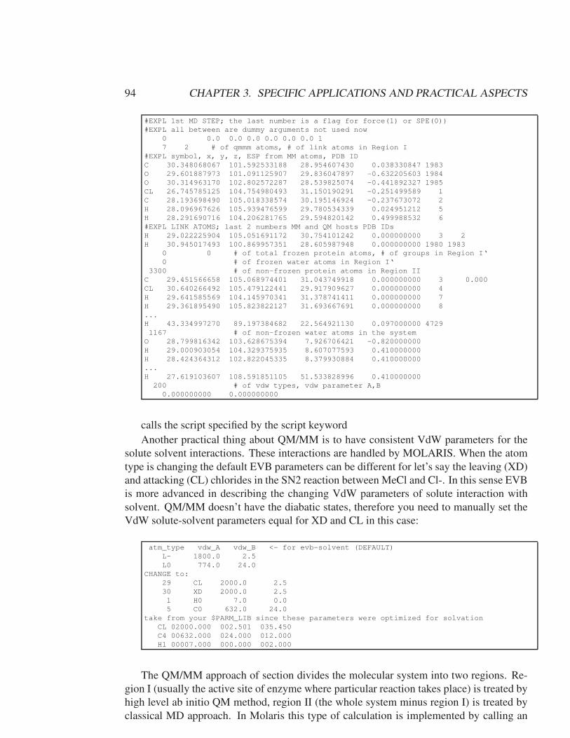
94 CHAPTER 3. SPECIFIC APPLICATIONS AND PRACTICAL ASPECTS
#EXPL 1st MD STEP; the last number is a flag for force(1) or SPE(0))
#EXPL all between are dummy arguments not used now
0 0.0 0.0 0.0 0.0 0.0 0.0 1
7 2 # of qmmm atoms, # of link atoms in Region I
#EXPL symbol, x, y, z, ESP from MM atoms, PDB ID
C 30.348068067 101.592533188 28.954607430 0.038330847 1983
O 29.601887973 101.091125907 29.836047897 -0.632205603 1984
O 30.314963170 102.802572287 28.539825074 -0.441892327 1985
CL 26.745785125 104.754980493 31.150190291 -0.251499589 1
C 28.193698490 105.018338574 30.195146924 -0.237673072 2
H 28.096967626 105.939476599 29.780534339 0.024951212 5
H 28.291690716 104.206281765 29.594820142 0.499988532 6
#EXPL LINK ATOMS; last 2 numbers MM and QM hosts PDB IDs
H 29.022225904 105.051691172 30.754101242 0.000000000 3 2
H 30.945017493 100.869957351 28.605987948 0.000000000 1980 1983
0 0 # of total frozen protein atoms, # of groups in Region I‘
0 # of frozen water atoms in Region I‘
3300 # of non-frozen protein atoms in Region II
C 29.451566658 105.068974401 31.043749918 0.000000000 3 0.000
CL 30.640266492 105.479122441 29.917909627 0.000000000 4
H 29.641585569 104.145970341 31.378741411 0.000000000 7
H 29.361895490 105.823822127 31.693667691 0.000000000 8
...
H 43.334997270 89.197384682 22.564921130 0.097000000 4729
1167 # of non-frozen water atoms in the system
O 28.799816342 103.628675394 7.926706421 -0.820000000
H 29.000903054 104.329375935 8.607077593 0.410000000
H 28.424364312 102.822045335 8.379930884 0.410000000
...
H 27.619103607 108.591851105 51.533828996 0.410000000
200 # of vdw types, vdw parameter A,B
0.000000000 0.000000000
calls the script specified by the script keywordAnother practical thing about QM/MM is to have consistent VdW parameters for the
solute solvent interactions. These interactions are handled by MOLARIS. When the atomtype is changing the default EVB parameters can be different for let’s say the leaving (XD)and attacking (CL) chlorides in the SN2 reaction between MeCl and Cl-. In this sense EVBis more advanced in describing the changing VdW parameters of solute interaction withsolvent. QM/MM doesn’t have the diabatic states, therefore you need to manually set theVdW solute-solvent parameters equal for XD and CL in this case:
atm_type vdw_A vdw_B <- for evb-solvent (DEFAULT)
L- 1800.0 2.5
L0 774.0 24.0
CHANGE to:
29 CL 2000.0 2.5
30 XD 2000.0 2.5
1 H0 7.0 0.0
5 C0 632.0 24.0
take from your $PARM_LIB since these parameters were optimized for solvation
CL 02000.000 002.501 035.450
C4 00632.000 024.000 012.000
H1 00007.000 000.000 002.000
The QM/MM approach of section divides the molecular system into two regions. Re-gion I (usually the active site of enzyme where particular reaction takes place) is treated byhigh level ab initio QM method, region II (the whole system minus region I) is treated byclassical MD approach. In Molaris this type of calculation is implemented by calling an

3.4. USING ENZYMIX 95
external QM program (e.g. Gaussian) that provides quantum mechanical energies, chargesand forces. The charges and forces are then used to update classical force field. Let us havea look at some practical aspects of QMMM run.
Request for QMMM calculation is specified in the input file by "qmmm" keyword inmd_parm level. Currently, this feature is supported only for AC type calculations. Thesnippet of input file below shows the most important QMMM related keywords.
md_parm
qmmm
qmmm_in filename
qmmm_out filename
script filename
cl_elec
end
end
Before calling the external QM program, Molaris writes out a file with data describingactual configuration of the system at given step. The name of this file is given by theparameter of "qmmm_in" keyword. A c-shell script parses the qmmm_in file and thenruns an external QM software (e.g. Gaussian). The parameter of the keyword "script"is used as the name of the c-shell script called by Molaris. This script has to be writtenby user since it needs to be tailored for each specific QM software that the user is using.After external QM calculation is finished Molaris reads results from the file specified by"qmmm_out" keyword and performs another MD step with updated force field. It is againuser’s responsibility that the script parses the output of external QM program and createsthe qmmm_out file.
The qmmm_in and qmmm_out files have to conform to a strict format. The qmmm_infile that is created by Molaris before calling external QM program contains following in-formation:
step_number total_energy something?
n_atoms_of_region_I
atom_name x y z charge something?
....
....
....
....
n_atoms_of_region_II
x y z charge
....
....
....
....
n_atoms_of_water_region
x y z charge
....
....
....
....
The environment of the region I is represented by point charges in external quantummechanical calculation. This is why region II and water region sections contains onlycoordinates and charges and not atom names. The energies are specified in kcal/mol, coor-dinates in A.

96 CHAPTER 3. SPECIFIC APPLICATIONS AND PRACTICAL ASPECTS
The qmmm_out file created by the c-shell script has following format:
qm_energy_of_region_I
force_x force_y force_z
....
....
....
....
....
qm_charge
....
....
....
....
....
The energy of region I is total energy [kcal/mol] that includes also interaction withenvironment. Forces are specified in kcal/mol/A. Each line in force and charges sectionscorresponds to the atom of region I in the same order like in qmmm_in file.
3.4.10 All-atom LRA results
In addition to the above treatment you can obtain automatic all-atom LRA results as a by-product of running PDLD/S-LRA calculations. The corresponding results are found in themd_lra.out file (see the section 3.5).
3.4.11 Restraint Release Approach calculations (RRA)
In section 2.1.11, we explain how ENZYMIX can be used to evaluate the free energy of re-leasing a restraint, and how this property may be used to calculate the entropic contributionin biomolecular systems. To demonstrate these features on a practical example, we look atthe reaction calaysed by alcohol dehydrogenase which is shown in figure 3.10
1RJW-relax.pdb
enzymix
pre_enz
setcrg 86 1.0
end
evb
evb_state 2 1.0 0.0 1
rest_in ./restfq_000.60000
evb_atm 6 0.28 N+ 0.27 N+
evb_atm 12 0.06 C+ -0.19 C+
evb_atm 19 -0.12 C+ -0.25 C+
evb_atm 27 0.03 C+ 0.31 C0
evb_atm 33 -0.14 C+ -0.34 C+
evb_atm 37 0.01 C+ -0.26 C+
evb_atm 39 0.68 C+ 0.76 C+
evb_atm 41 -0.88 N+ -0.97 N+
evb_atm 42 -0.48 O0 -0.7 O0
evb_atm 58 0.17 H0 -0.02 H0
evb_atm 62 0.45 H0 0.4 H0

3.4. USING ENZYMIX 97
Figure 3.10: A schematic of the reaction catalyzed by alcohol dehydrogenase (ADH), which illustrates thefact that in this reaction (left to right), entropy changes could reflect restrictions on the fluctuations of theprotein dipoles in the highly polar reactant state, relative to the partially polar TS, which would lead to apositive ∆S 6=. If the temperature is raised, this would release some of the frozen motions in the reactantstate, which would be expected to result in a less positive ∆S 6=.

98 CHAPTER 3. SPECIFIC APPLICATIONS AND PRACTICAL ASPECTS
evb_atm 64 0.17 H0 0.2 H0
evb_atm 65 0.2 H0 0.16 H0
evb_atm 66 0.19 H0 0.21 H0
evb_atm 70 0.38 H0 0.43 H0
evb_atm 71 -0.96 O--0.54 O0
evb_atm 72 -0.18 C+ -0.21 C+
evb_atm 73 -0.15 C+ -0.09 C+
evb_atm 74 0.5 C0 0.39 C+
evb_atm 75 -0.26 C+ -0.11 C+
evb_atm 76 -0.09 C+ -0.16 C+
evb_atm 77 -0.26 C+ -0.08 C+
evb_atm 78 0.18 C+ 0.03 C+
evb_atm 79 -0.14 H0 0.05 H0
evb_atm 80 0.13 H0 0.16 H0
evb_atm 81 0.1 H0 0.14 H0
evb_atm 82 0.11 H0 0.15 H0
evb_atm 83 0.09 H0 0.15 H0
evb_atm 84 0.08 H0 0.13 H0
evb_atm 85 -0.14 H0 -0.02 H0
evb_bnd 0 6 12
evb_bnd 0 6 37
evb_bnd 0 12 64
evb_bnd 0 12 19
evb_bnd 0 19 27
evb_bnd 0 19 39
evb_bnd 0 39 41
evb_bnd 0 39 42
evb_bnd 0 41 70
evb_bnd 0 41 62
evb_bnd 0 27 58
evb_bnd 0 27 33
evb_bnd 0 33 65
evb_bnd 0 33 37
evb_bnd 0 37 66
evb_bnd 0 74 71
evb_bnd 0 74 79
evb_bnd 0 74 78
evb_bnd 0 78 72
evb_bnd 0 78 77
evb_bnd 0 72 80
evb_bnd 0 72 73
evb_bnd 0 73 81
evb_bnd 0 73 75
evb_bnd 0 75 82
evb_bnd 0 75 76
evb_bnd 0 76 83
evb_bnd 0 76 77
evb_bnd 0 77 84
evb_bnd 2 27 85
evb_bnd 1 85 74
evb_d_con 74 27 3.0 10.0 0

3.4. USING ENZYMIX 99
md_parm
stepsize 0.001
temperature 300.0
nsteps 10000
log_write_fq 1000
region2a_r 16
water_r 16
langevin_r 18
movie_co all
movie_fq 1000
constraint_1 10.0
constraint_2 10.0
rms_residue 1 to 406
rest_constr
rr_res_contrib
rr_forceconst 10.0 9.5 9.0 8.5 8.0 7.5 7.0 0.4 0.3 0.2 0.1 0.05 0.03
rr_const region2 500
rr_const region1 500
quasih_entropy 10 region1+2
end
end
end
end
end
end
end
In the input template provided, we simply load a previously created restart file, andperform our RR calculations on either of the evb states. The RR calculations are car-ried out for both the release of the constraint on the system, as well as the collectionof all necessary data at the maximum value of the constraint for the QH approximation.More specifically, the example given applies the constraints on all atoms of region1 andregion2, rr_const region1 and rr_const region2. The keyword rr_forceconst is re-quired for defining a list of individual values of the constraint (and is currently limited to150 values). That means, the system will be sampled for each of the force constants inrr_forceconst and the file rr_const_dG.out that contains the FEP data from maximumto minimum rr_forceconst will be created upon successful termination. The estimate forthe free energy of releasing the constraints is printed in kcal/mol at the bottom of this file:
Average total dG from forward and backward mapping = -260.500
By default MOLARIS also generates files listing the individual contributions to the FEPfor RR free energies (see rr_const_reg1_dG.out and rr_const_reg2_res_dG.out for con-tributions of region 1 and 2).The separate data collection for the quasiharmonic contribution is enabled through the key-word quasih_entropy 10 region1+2, which, in the present case, would collect data for

100 CHAPTER 3. SPECIFIC APPLICATIONS AND PRACTICAL ASPECTS
all atoms of region1 and region2, for every 10 MD steps. The value of the force constantused by the QH is supplied by the keywords constraint_1 and constraint_2, however,these two keywords are only active for the QH analysis, they will not be used for theRR part of the calculations as rr_forceconst overrides them. Upon termination, the filesentropy.info and entropy.dat will be created. These binary files are then run with theprogram xquasih_entropy_dsyev:
xquasih_entropy_dsyev < entropy.input > entropyQH.out
Here, entropy.input is a simple text file that contains 3 lines:
entropy.info
entropy.dat
1000
which tells the program the names of the necessary binaries created previously, fol-lowed by an integer that specifies the cutoff freqency. The resulting file entropyQH.outnow contains at the bottom our QH analysis estimate for −T∆S:
-------------------------------------------------------
quasiharmonic entropy(J/mol/K) = 1618.87
-TS(kcal/mol, T=300.0K) = -94.43
-------------------------------------------------------
The current −T∆S for the current simulations is then simply the sum of the RR andthe QH. Now, the idea of the RR approach lies in the varational minimization that, inprinciple, should eliminate any enthalpic contribution. In other words, having performedthese calculations on a series of trajectories for any two states, then allows us to find theabsolute minimum between them, and this final number is the estimated −T∆S that shouldcontain only entropic contributions.Since the RR approach requires sampling over many independent trajectories in order togive reliable results, it is important to keep in mind how MOLARIS calculates the constraintenergies. Therefore, it is highly recommended to use the rest_constr keyword
3.4.12 FEP calcaultion of mutating dummy atoms
This is test for now. hanwoolyThe FEP calculation is also often used to simulate an alchemical transformation which
may eventually mutate real atoms with residual charges and vdW parameters to dummyatoms. For example, one would want to see the effect of changing a hydroxyl group to ahydrogen in the system. In this case, the oxygen and the hydrogen of the hydroxyl groupwill be slowly changed to a hydrogen and a dummy atom, repectively. However, it hasbeen known that when there are vanishing atoms during the FEP calculation, the calcula-tion leads to a disastrous numerical explosion very often, especially when λ approaches 0or 1 very close. When the vdW parameters of the vanishing atom becomes very small, itoccasionally gets extremely close to other atoms while it still carries residual charges.Several approaches have been adopted to avoid this issue. It is usually recommended to

3.4. USING ENZYMIX 101
decouple the electrostatic and vdW calculation. Speicifically, one could first change theresidual charges to zero over λ , then decrease the vdW parameters to zero. However, eventhough this would resolve the electrostatic explosion, the calculation may still experiencevdW catastrophe around the last frame. In this case, the last frame can be divided furtherwith a smaller δλ to moderate the vdW changing rate.However, the approaches above still do not guarantee the stability and also they are compu-tationally more expensive. The nature of the problem stems from the fact that the repulsionpart of the vdW function increase exponentially. We need to avoid the vdW clash but wealso need to sample the prohibited space by the exponential repulsion part of the vdWfunction. In this case, no matter how small δλ is used, the problem may still remains. vanGunsteren introduced a lambda dependent vdW fucntion which scales down the potentialsas λ approaches to 0 or 1.In ENZYMIX, a similar approach has been implemented with keywords, use_vdw_erand use_vdw_er_atom . The example usage of this keyword is shown below.
./rb69_original.pdb
enzymix
evb
evb_state 2 1 0
map_pf 51 1 2
evb_atm 57 -0.573 O0 0.072 H0
evb_atm 73 0.447 H0 0.000 DO
evb_bnd 0 57 73
rest_in relaxed.res
rest_out fep_mutation.res
md_parm
temperature 310
stepsize 0.001
nsteps 10000
use_vdw_er_atom 1.8 73 1
use_vdw_er_atom 2.3 57 1
constraint_1 0.3
constraint_2 0.03
end
end
end
This keyword uses a modified vdW function so that a constant force is used below acertain distance cut-off value defined by users. That is,
F (r) =
{
−dV/dr = 12A/r13 + 6B/r7, if r > r_cut
F (r_cut) = constant, if r <= r_cut(3.4)
Thus, the potential energy can be analgously derived as follows:
V (r) =
A/r12 +B/r6, if r > r_cut
V (r_cut) +∫ r
r_cut−F (r) if r <= r_cut
= V (r_cut) + (r_cut− r) ∗ F (r_cut),
(3.5)

102 CHAPTER 3. SPECIFIC APPLICATIONS AND PRACTICAL ASPECTS
Therefore, for r < r_cut, the potential energy increases linearly with a slope given byF(r_cut). The comparison between the original Lennard-Jones potential and the modifiedpotential are shown in Figure 3.11 .
Figure 3.11: The original Lennard-Jones potential/force and the modified potential/force.
3.5 Using POLARIS
Before entering in this section it is useful to make a general comment about the PDLDcalculations. For most of the calculations below, MOLARIS offers a great flexibility inchosing all kind of parameters and also in defining the regions of the system and theircharges. In the PDLD cycle, we always compare the solvation obtained from the actualcharged system to the uncharged one. This can be controlled by reading the PDLD filecreated in a previous run and/or by using the corresponding keywords in the POLARISlevel of the input file. In this sense, a note of caution must be said concerning the definitionof the charged-uncharged systems. POLARIS always compares a charged system to theuncharged one, which means that state A in the PDLD cycle is the charged one and state Bis the uncharged system. With this in mind we can start describing the different calculationsthat can be done at the POLARIS level in MOLARIS.
3.5.1 Calculating solvation energies of molecules in water
POLARIS provides a reliable and efficient way to calculate the solvation energies of smallmolecules. This type of calculation has been extensively validated (e.g.see refs. [71, 13]and Table 3.12). For doing this we just need to use the solv_pdld keyword in POLARISand follow the menu. In a similar way you may calculate the solvation energy of a small

3.5. USING POLARIS 103
protein. You may try this option by taking the dodecapeptide of small.pdb in pl_solv_pdld.In view of the large interest in solvation of small molecules, we include in the demo ourbenchmark (solv_benzene). The input file benzene.inp in solv_benzene directory in thedemo looks as follows:
../pdb/benzene.pdb
polaris
solv_pdld
reg1_res 1
config 1 0
end
end
end
Note that for a molecule in water we do not need any configuration average. A typicalfinal output is given below for benzene from running POLARIS with benzene.inp. PDLDRESULTS:
*************************PDLD MICROSCOPIC ESTIMATE
*************************
SOLVATION OF REGION 1 IN WATER (STATE B->A): GAS->WATER(FOR STATE A ):
dlangevin -1.37 dlangevin -1.37
dhydro -0.62 dhydro 6.10
dborn 0.00 langevin VDW -5.66
dborn 0.00
dGw (without dhydro ) -1.37 dG -0.93
The above output gives the solvation of the benzene molecule in several ways. Wealso give the free energy associated with changing the residual charges of our moleculefrom those of state A to those of state B. The absolute solvation energy is given underGAS->WATER(FOR STATE A) and includes the hydrophobic (dhydro), van der Waalsand Born contributions.
The calculated and observed solvation energies are given in Table 3.26 and Fig. 3.12.
# name dGexp dGcalc dGexp-calc # name dGexp dGcalc dGexp-calc1 methane 2.00 2.16 -0.16 51 3-methyl-2-butanone -3.24 -3.07 -0.172 ethane 1.83 1.9 -0.07 52 2-hexanone -3.29 -2.93 -0.363 propane 1.95 1.85 0.10 53 4-methyl-2-pentanone -3.06 -2.74 -0.324 butane 2.08 2.21 -0.13 54 2-heptanone -3.04 -2.57 -0.475 isobutane 2.32 2.27 0.05 55 4-heptanone -2.92 -2.66 -0.266 pentane 2.33 2.36 -0.03 56 2,4-dimethyl-3-pentanone -2.74 -2.82 0.087 2-methylbutane 2.38 2.24 0.14 57 acetophenone -4.58 -4.14 -0.448 hexane 2.48 2.51 -0.03 58 acetaldehyde -3.50 -3.86 0.369 benzene -0.93 -0.76 -0.11 59 propanal -3.44 -3.58 0.1410 biphenyl -2.64 -1.74 -0.90 60 butanal -3.17 -2.97 -0.20

104 CHAPTER 3. SPECIFIC APPLICATIONS AND PRACTICAL ASPECTS
11 methanol -5.11 -5.66 0.55 61 pentanal -3.03 -3.21 0.1812 ethanol -5.01 -5.26 0.25 62 hexanal -2.81 -2.84 0.0313 1-propanol -4.82 -5.44 0.62 63 heptanal -2.67 -2.48 -0.1914 1-butanol -4.71 -5.27 0.56 64 octanal -2.29 -2.17 -0.1215 1-pentanol -4.47 -5.13 0.66 65 acetic acid -6.70 -6.26 -0.4416 3-methyl-1-butanol -4.42 -4.83 0.41 66 propionic acid -6.47 -5.26 -1.2117 2,3-dimethyl-2-butanol -3.91 -4.23 0.32 67 butanoic acid -6.35 -7.31 0.9618 4-heptanol -4.00 -2.97 -1.03 68 ethyl formate -2.64 -5.54 2.9019 cyclopentanol -5.49 -5.3 -0.19 69 methyl acetate -3.31 -3.4 0.0920 cyclohexanol -5.47 -5.2 -0.27 70 ethyl acetate -3.09 -2.86 -0.2321 cycheptanol -5.48 -5.08 -0.40 71 methyl propionate -2.93 -3.05 0.1222 phenol -6.61 -6.18 -0.43 72 propyl acetate -2.85 -2.81 -0.0423 2-methyl phenol -5.87 -5.33 -0.54 73 isopropyl acetate -2.64 -2.05 -0.5924 4-methyl phenol -6.13 -5.58 -0.55 74 ethyl propionate -2.80 -2.34 -0.4625 p-t-butyl phenol -5.92 -6.05 0.13 75 methyl butanoate -2.83 -2.55 -0.2826 dimethyl ether -1.89 -2.24 0.35 76 isopropyl propionate -2.22 -2.47 0.2527 diethyl ether -1.63 -1.78 0.15 77 methyl hexanoate -2.49 -1.93 -0.5628 methyl propyl ether -1.66 -1.5 -0.16 78 methyl benzoate -4.28 -3.58 -0.7029 isopropyl methyl ether -2.00 -1.8 -0.20 79 chloromethane -0.56 0.11 -0.6730 ethyl propyl ether -1.81 -0.86 -0.95 80 chlorobenzene -1.12 -0.03 -1.0931 t-butyl methyl ether -2.21 -2.16 -0.05 81 nitroethane -3.71 -2.04 -1.6732 dipropyl ether -1.15 -0.4 -0.75 82 1-nitropropane -3.34 -1.57 -1.7733 diisopropyl ether -0.53 -0.54 0.01 83 2-nitropropane -3.14 -1.06 -2.0834 dibutyl ether -0.83 -0.69 -0.14 84 nitrobenzene -4.11 -3.93 -0.1835 methylamine -4.56 -3.92 -0.64 85 o-methyl nitrobenzene -3.59 -2.89 -0.7036 ethylamine -4.50 -4.94 0.44 86 m-methyl nitrobenzene -3.45 -2.44 -1.0137 propylamine -4.39 -4.49 0.10 87 N-methylacetamide -10.20 -10.14 -0.0638 butylamine -4.29 -4.37 0.08 88 m-nitrophenol -10.14 -8.29 -1.8539 pentylamine -4.09 -3.77 -0.32 89 p-nitrophenol -11.92 -9.12 -2.8040 hexylamine -4.03 -3.31 -0.72 90 alanine dipeptide -16.96 -16.59 -0.3741 dimethylamine -4.28 -4.61 0.33 91 aniline -4.90 -2.38 -2.5242 diethylamine -4.07 -3.49 -0.58 92 toluene -0.90 0.27 -1.1743 dipropylamine -3.66 -4.18 0.52 93 Br- -72.00 -74.35 2.3544 dibutylamine -3.33 -3.15 -0.18 94 Cl- -76.60 -77.01 0.4145 trimethylamine -3.24 -2.87 -0.37 95 F- -105.80 -105.32 -0.4846 pyridine -4.70 -4.52 -0.18 96 I- -62.60 -66.95 4.3547 2-propanone -3.97 -3.78 -0.19 97 Na+ -100.30 -98.70 -1.6048 2-butanone -3.63 -3.67 0.04 98 NH4 -74.94 -77.80 2.8649 2-pentanone -3.53 -2.91 -0.6250 3-pentanone -3.41 -3.68 0.27
Table 3.26: POLARIS solvation free energies (in water) for a benchmark of neutral andcharged molecules. Energies in kcal/mol
3.5.2 Calculating solvation free energies using ab initio chargesIn addition to the use of POLARIS group charges (see Section 2.2.4) we provide the well-calibrated and very convenient ChemSolprogram (see ref. [61]) that evaluates accurately solvation free energies using the results of GAUSSIAN or related ab initio programs.Refer to the ChemSol manual on our website for more details.
3.5.3 Solvation energy of a part of a macromoleculeIn determining electrostatic free energies of charged groups in proteins the key difficulty is not the interaction between charges, but it isin calculating the “self-energy” or “solvation energy” (the energy of moving the charged group into its protein site from vacuum). Thisenergy is best defined relative to the corresponding solvation energy in water, i.e.:
∆Gpsol = (∆Gp
sol −∆Gwsol) + ∆Gw
sol = ∆∆Gw→psol +∆Gw
sol (3.6)
where w and p designate water and protein respectively.POLARIS uses eq. (3.6) when estimates solvation energies of charged groups in macromolecules, utilizing both the semi-
microscopic PDLD/S and the microscopic PDLD methods. An example of such a calculation is provided in demo pl_solv_pdld. In thisdemo, the solvation free energy of the positively charged NH3
+ group of a lysine residue in a dodedcapeptide is calculated. The inputfile looks like:

3.5. USING POLARIS 105
-120 -100 -80 -60 -40 -20 0 20
-120
-100
-80
-60
-40
-20
0
20
Experimental ∆Gsolv
Ca
lcu
late
d ∆
Gsolv
Figure 3.12: Correlating calculated and observed solvation energies for the benchmark of Table 3.26
../pdb/small.pdb
polaris
pre_pol #preparing polaris run
ionres 12 #ionizes the given residue
end
solv_pdld #calculating solvation energies
reg1_atm 176 to 179 #specifies region I atoms
config 0 3 #calculation on 3 MD-generated configurations
end
end
end
The output file includes results from the all-atom LRA generation (see section 2.2.8)of different configurations. This is done for n configurations for the charge and unchargedstate. The corresponding average energy contributions for the protein run looks like:

106 CHAPTER 3. SPECIFIC APPLICATIONS AND PRACTICAL ASPECTS
Average energies for AC atoms:
----------------------------------
************ average values for all the steps ************(the first 100 steps excluded)
State A State B
Coulombic/acp total : -47.90 0.00
Intra ac group | 0.00 0.00|breakdown Inter ac group | 0.00 0.00|
(vqq)
ac-protein | -47.90 0.00|(vqu)
Coulombic/wat : -108.19 0.00
Induced/pro : 0.00 0.00
Induced/wat : 0.00 0.00
Vdw/pop total : 0.87 0.87
Intra ac group | 0.00 0.00|breakdown Inter ac group | 0.00 0.00|
ac-protein | 0.87 0.87|
Vdw/wat : 6.30 6.30
Hb/pro : -2.88 -2.88
Hb/wat : 0.00 0.00
langevin : -19.20 -18.15
born : -8.78 -0.52
Total(elec only) : -186.95 -21.55
A --> B (elec only) : 165.40
for each configuration we calculate the PDLD and PDLD/S energies. The typical outputfor this part looks like:
region I charges
atom # x y z qa qb code rp
176 42.400 32.100 15.400 -0.080 0.000 33 2.50
177 41.780 31.630 16.028 0.360 0.000 1 1.50
178 43.165 32.496 15.908 0.360 0.000 1 1.50
179 41.908 32.819 14.909 0.360 0.000 1 1.50
total charge for region I state A: 1.000
total charge for region I state B: 0.000
total charge in region II: 0.000
This gives the number of the Region I atoms, the xyz-coordinates, the charges in stateA (qa) and in state B (qb) as well as the PDLD atom code and the vdW radius (rp). Notethat the charges for state B are all zero. Now follows the calculation of the solvation freeenergy of these Region I atoms in water. This calculation gives the Langevin free energyin water. The resulting solvation energy is used in the subsequent calculations.
The next step is the calculation of the energies for the Region I atoms in protein (RegionII) and water. Here, we also find energy contributions in state B resulting from the non-zero charge of the Region II atoms. The final result is given in the semi-macroscopic

3.5. USING POLARIS 107
PDLD/S approximation and also in the microscopic form. The PDLD/S result should lookas follows:
******************************PDLD SEMI-MACROSCOPIC ESTIMATE
******************************
effective dielectric 2 4 6 8 20 40 80
epsilon_p(e_p)
-dG in water 40.43 20.16 13.41 10.03 3.87 1.89 0.89
(e_p -> e_80)
dvqmu(e=e_p) -24.93 -12.47 -8.31 -6.23 -2.49 -1.25 -0.62
dlangevin(e_p->e_80) -12.99 -6.50 -4.33 -3.25 -1.32 -0.66 -0.33
dbulk(born,e_p->e_80) -4.04 -1.97 -1.28 -0.93 -0.31 -0.10 0.00
ddG(water -> protein) -1.53 -0.77 -0.51 -0.38 -0.25 -0.12 -0.06
(e=e_p)
These PDLD/S data are based on a special macroscopic scaling of the microscopicPDLD results (see Section 2.2.7). The meaning of the entries in the table is as follows.dG in water is the solvation free energy in water. This value is calculated as the sum ofthe Boltzmann averaged langevin energy difference of -71.43 and the difference in Bornenergy between configuration A and B (total Born energy difference -8.22) multiplied by(1/ε – 1/80). The next lines contain the results from the calculation of Region I in proteinand water. Uqµ is the charge-charge interaction between the Region I atoms and the proteinatoms. The value of dvqmu is the difference between the Uqµ of configurations A and Bmultiplied by 1/ε. Here, it is the value of Uqµ of state A only, as the Uqµ in state B is zerobecause of the residual charges being zero. The lines designated as Langevin and bulkenergies correspond to the difference in the microscopic solvation energies of the entiremacromolecule with the charged and uncharged states of region I (the ∆∆Gw
p term ineq. (2.61) multiplied by (1/ε – 1/80). The resulting change in solvation free energy whentransferring the Region I atoms from water to protein, ddG(water -> protein, is given asthe sum of dG in water and the (e_p->e_80) contributions, which are dvqmu, dlangevin,and dbulk. The value of -2.45 (at ε=4) means that the solvation energy of Region I atomsis bigger in the protein than in water.The PDLD/S result is followed by the microscopic PDLD result:
*************************PDLD MICROSCOPIC ESTIMATE
*************************
SOLVATION OF REGION 1 IN WATER (STATE B->A): GAS->WATER(FOR STATE A ):
dlangevin -71.31 dlangevin -71.31
dhydro -3.74 dhydro 0.00
dborn -8.20 langevin VDW -1.71
dborn -8.20

108 CHAPTER 3. SPECIFIC APPLICATIONS AND PRACTICAL ASPECTS
dGw (without dhydro ) -79.51 dG -81.22
SOLVATION OF REGION I IN PROTEIN + WATER:
dvqmu -49.87
dvqalpha -0.10
dlangevin -26.36
dhydro -3.45
dborn -8.28
dGp (without dhydro ) -84.61
ddG (water -> protein) = dGp-dGw -5.10
After the run is completed we have a concise summary of the relevant results in twooutput files. The first file solv_pdld.out gives the average PDLD/S-LRA results:
Results averaged over all configs (charged and uncharged)
effective dielectric 2 4 6 8 20 40 80
epsilon_p(e_p)
-dGw in water 40.59 20.24 13.46 10.07 3.90 1.90 0.90
dvqmu(e=e_p) -15.24 -7.62 -5.08 -3.81 -1.52 -0.76 -0.38
dlangevin(e_p->e_80) -19.97 -9.98 -6.66 -4.99 -1.91 -0.96 -0.48
dbulk(born,e_p->e_80) -4.03 -1.96 -1.27 -0.93 -0.31 -0.10 0.00
dGp in protein -39.24 -19.57 -13.01 -9.73 -3.74 -1.82 -0.86
ddG_elec=dGp-dGw 1.35 0.68 0.45 0.34 0.15 0.08 0.04
---------------------------------------------------------------------
SOLVATION ENERGY OF REGION I (ddG water->protein)
solvation for new configurations :
(with reorganization energy)
********************************************PDLD SEMI-MACROSCOPIC ESTIMATE FOR SOLVATION
********************************************(dielectric constant=4)
ddG solvation (water -> protein) for structure 1 0.41
ddG solvation (water -> protein) for structure 2 1.30
ddG solvation (water -> protein) for structure 3 0.33
----------------------------------------------
average ddG(water -> protein+water,pdld/s) = 0.68
The second useful output summerizes the all-atom LRA results. The corresponding filemd_lra.out looks like:

3.5. USING POLARIS 109
LRA from structures of all steps of each configuration
(L)w for region I in water:
average over state A and B average over state B
------- ------------------------------------------------ -----------------------------
config vQmu vindu vQw lgvn born dG(elec) vdw_L/P vdw_L/W dG(nonelec)
....... ....... ....... ....... ....... ................ ....... ........ ............
1 0.0 -77.9 0.0 -8.2 -86.0 2.1 2.1
average 0.0 -77.9 0.0 -8.2 -86.0 2.1 2.1
(L)pw for region I in protein and water:
average over state A and B average over state B
------- ------------------------------------------------ -----------------------------
config vQmu vindu vQw lgvn born dG(elec) vdw_L/P vdw_L/W dG(nonelec)
....... ....... ....... ....... ....... ................ ....... ........ ............
1 -34.6 0.0 -38.7 -0.3 -8.3 -81.8 1.1 1.4 2.4
2 -33.2 0.0 -39.7 -0.1 -8.4 -81.3 1.0 1.0 2.1
3 -24.9 0.0 -51.1 -0.2 -8.0 -84.3 0.7 1.8 2.5
average -30.9 0.0 -43.2 -0.2 -8.2 -82.5 0.9 1.4 2.3
(L)pw-(L)w:
average over state A and B average over state B
------- ------------------------------------------------ -----------------------------
config vQmu vindu vQw lgvn born dG(elec) vdw_L/P vdw_L/W dG(nonelec)
....... ....... ....... ....... ....... ................ ....... ........ ............
average -30.9 0.0 34.7 -0.2 -0.1 3.5 0.9 -0.7 0.3
LRA electrostatic energy:
DDG = ddG(elec) = 3.5
3.5.4 Calculations of pKa’s of ionizable groups in proteins
One of the most important examples of electrostatic calculations of macro molecules isprovided by the calculation of pKa’s of ionized groups in proteins.
These quantities give very valuable information about the electrostatic energies in pro-tein sites and can serve as a unique benchmark for electrostatic calculations in proteins (formore details see ref. [67]). The evaluation of the ionization states requires one to determinethe intrisic pKa (the pKa when all other ionized groups are uncharged) and the shift of pKa
due to the charge-charge interaction. The evaluation of the intrinsic pKa by fully micro-scopic FEP or LRA calculations is quite challenging[7, 108, 34] and may involve errorsof several pKa units. In many cases and particularly in cases of surface groups one obtain

110 CHAPTER 3. SPECIFIC APPLICATIONS AND PRACTICAL ASPECTS
more stable results by using semimacroscopic models such as the PDLD/S-LRA and PBmethods. The problem is, however, to get reliable results for groups in the protein interiors(see discussion in ref. [67]).
In calculating pKa’s one has to consider the thermodynamic cycle of Fig. 2.11 and toevaluate the two contributions; (i) the self energy of the ionized group that reflects the freeenergy of charging this group in its protein site when all other groups are in their neutralform and (ii) the energy of interaction between the ionized residues. As was argued repeat-edly and demonstrated by analyzing many experimental results, the effect of the interactionbetween ionized groups is largely screened and the most important contribution to pKa’s inprotein is the self energy term that reflects the effect of the polar groups around the site ofthe given ionized residue. In general we can express the pKa of each group of the proteinby
pKpa,i = pKp
app,i = pKpint,i +∆pKcharges
a,i (3.7)
where pKapp,i is the actual (apparent) pKa of the ith group, pKint,i is the so-called intrinsicpKa, (this is the pKa that the ith group in the protein would have when all other groups arein their neutral states) and ∆pKcharges
a,i represents the effects of the other ionized groups.Using eq’s 2.48,2.49 and 2.51 we can write
pKpapp,i = pKw
a,i −qi
2.3RT∆∆Gw→p
self,i +∆pKchargesa,i (3.8)
The ∆pKchargesa,i term is given by:
∆pKchargesa,i = −
q
2.3RT
∑
j 6=i
∆Gpij (3.9)
where the ∆Gpij represents the interaction with the jth ionized group.
POLARIS can calculate the ∆∆Gself,i term (and the corresponding pKpint,i) microscop-
ically by the PDLD, LRA or FEP methods (see below). However, at present the most stableresults are obtained by the PDLD/S-LRA approach (Section 2.2.8).
The effects of other ionized groups, ∆pKchargesa,i , is usually evaluated macroscopically,
using:
∆Gpij = 332qi
∑
j 6=i
qjrijεij
(3.10)
Where qi and qj are the actual charges of the ith and the jth ionizable group and it can be0 or -1 for acids and 0 or 1 for bases. rij is the distance between the charge centers of theith and jth groups and εij is an effective dielectric constant (see next section). The term canbe evaluated self-consistently by macroscopic approximations and is considered in Section3.5.6, which deals with titration curves. This term should be evaluated only after one has areasonable idea about the intrinsic pKa term.
In order to familiarize yourself with the way POLARIS calculates pKas it is useful toconsider the demo pl_pka_pdld which evaluates the pKa of Asp_3 in BPTI. The input filelooks like this:

3.5. USING POLARIS 111
../pdb/bpti.pdb
polaris # enter the POLARIS module
pre_pol
set_opt # set some parameters for PDLD
rg 18.0
ndxp 3
itl 10
end
end
pKa_pdld # enter the pKa calculation
reg1_res 3 # identify region I. Do pKa of residue 1
config 1 2 # configurations to be done
md_parm_r # relaxation dynamics
nsteps 300
end
md_parm_w # dynamics in water
nsteps 200
end
md_parm_p # dynamics in protein
nsteps 200
end
end
end
end
Here you have information from the MD run that generates the LRA conformation canbe used for microscopic LRA calculations.
State A State B
Coulombic/acp total : -10.76 0.00
Intra ac group | 0.00 0.00|breakdown Inter ac group | 0.00 0.00|
(vqq)
ac-protein | -10.76 0.00|(vqu)
Coulombic/wat : -151.44 0.00
Induced/pro : 0.00 0.00
Induced/wat : 0.00 0.00
Vdw/pop total : 7.62 7.62
Intra ac group | 0.07 0.07|breakdown Inter ac group | 0.00 0.00|
ac-protein | 7.55 7.55|
Vdw/wat : 11.52 11.52
Hb/pro : -0.11 -0.11
Hb/wat : 0.00 0.00
langevin : -44.89 -42.54
born : -10.46 -1.76
Total(elec only) : -217.66 -44.41
A --> B (elec only) : 173.25
In general we will have n runs for the charge and uncharged states.For each configuration we calculate the PDLD/S energies:
******************************PDLD SEMI-MACROSCOPIC ESTIMATE

112 CHAPTER 3. SPECIFIC APPLICATIONS AND PRACTICAL ASPECTS
******************************
effective dielectric 2 4 6 8 20 40 80
epsilon_p(e_p)
-dG in water 39.49 19.69 13.09 9.79 3.78 1.84 0.87
(e_p -> e_80)
dvqmu(e=e_p) -5.72 -2.86 -1.91 -1.43 -0.57 -0.29 -0.14
dlangevin(e_p->e_80) -29.40 -14.70 -9.80 -7.35 -2.83 -1.41 -0.71
dbulk(born,e_p->e_80) -4.25 -2.07 -1.34 -0.98 -0.33 -0.11 0.00
ddG(water -> protein) 0.11 0.06 0.04 0.03 0.05 0.03 0.02
(e=e_p)
The average PDLD semi-microscopic estimate for the pKa is calculated using the LRAapproach and the resulting treatment can be expressed as:
pKpa =
1
m
∑
m
{pKa,wat −1
2.303RT[1
2(ddGconfigA
w→p + ddGconfigBw→p )]} (3.11)
where m is the number of configurations.The averaged results are given in pKa_pdld.out, here we convert the PDLD/S energies
to intrinsic pKa.
----------------------------------------
Summary of pKa for the different configs
----------------------------------------
PDLD SEMI-MACROSCOPIC ESTIMATE FOR pKa
......................................
effective dielectric 2 4 6 8 20 40 80
epsilon_p(e_p)
pKa_intr for str. 1 4.52 4.21 4.11 4.05 3.99 3.94 3.92
pKa_intr for str. 2 4.87 4.39 4.22 4.14 4.00 3.95 3.93
------------------------------------------------------------------------
aver pKa_int 4.69 4.30 4.16 4.10 4.00 3.95 3.92
Finally, we use the intrinsic pKa (for ε = 4) and evaluate the apparent pKa.
estimated apparent pKa 3.77
The apparent pKa is obtained here automatically using default values for the pKas ofthe other ionizable groups. For a more systematic treatment you should use the titrationkeyword and the procedure described in section 3.5.6.

3.5. USING POLARIS 113
It should be noted that the default calculations of POLARIS neglect the contribution ofthe polar state (∆Gsol(AH)). This rather small contribution can be obtained by repeatingthe same procedure described above for the AH state. In this case the user should create anew PDB file with th eprotonated residue and repeat the calculations assigning the residualcharges of AH to state a. The resulting pKa (with pKw
a = 0) will correspond to the changein the pKa due to the inclusion of ∆Gw→p
sol (AH). This term should be simply added to thepreviously obtained pKa (the value obtained from the default calculations).
A benchmark for pKa calculations of Lysozyme is given in xxx(not done yet..)
Table 3.36: Calculated pKas of some of the ionizable groups in hen egg lysozyme (1hel and 2lzt)
1hel 2lzt
Res pKa(int) ∆pKa pKa(calc) pKa(int) ∆pKa pKa(calc) pKa(exp)ASP 18 4.07 -1.58 2.50 3.42 -0.97 2.45 2.9ASP 48 4.73 -1.24 3.49 3.70 -1.21 2.49 4.3ASP 52 6.23 -0.59 5.64 5.34 -0.85 4.49 3.6ASP 66 3.45 -0.45 3.01 5.29 0.05 5.34 2.0ASP 87 3.54 -1.06 2.48 3.12 -1.62 1.50 3.62ASP 101 4.84 -1.35 3.49 5.86 -1.37 4.49 4.12ASP 119 4.17 -1.67 2.50 3.50 -2.00 1.50 2.5GLU 7 5.09 -1.59 3.50 4.20 -1.70 2.50 2.6GLU 35 6.41 -0.94 5.47 7.01 -1.51 5.50 6.1
3.5.5 All-atom LRA calculations of pKas
Obtaining stable pKas from all-atom simulations is much more chalenging than the useof continuum models or the PDLD/S-LRA model. Since the results are not scaled and wehave to obtain almost a pe rfect balance between different contributions to the self energyof ionized group [65]. A t any rate, despite convergence difficulties it is useful to obtainmicroscopic all-atom results an d the simplest way is to obtain the corresponding LRAresults. These results are provided on the md _lra.out file generated automatically whenone uses the pka_pdld of POLARIS. Here however we are no t interested in the PDLD/Sresults but with the LRA results thus you should ask for only one config uration average(this will involve only one PDLD calculation) but you should use many steps for the MDaverages in water and in the protein. A typical demo is given in pl_pka_LRA (whichevaluates the pKa of Asp 3 in bpti) and the output given in the md_lra.out file looks like:
LRA from structures of all steps of each configuration
(L)w for region I in water:
average over state A and B average over state B
------- ----------------------------------------- -----------------------------
config vQmu vQw lgvn born dG(elec) vdw_L/P vdw_L/W dG(nonelec)
....... ....... ....... ....... ....... ......... ....... ........ ............
1 -78.0 -0.7 -8.2 -86.9 -1.7 -1.7
average -78.0 -0.7 -8.2 -86.9 -1.7 -1.7

114 CHAPTER 3. SPECIFIC APPLICATIONS AND PRACTICAL ASPECTS
(LP)w for region I+II in water:
average over state A and B average over state B
------- ----------------------------------------- -----------------------------
config vQmu vQw lgvn born dG(elec) vdw_L/P vdw_L/W dG(nonelec)
....... ....... ....... ....... ....... ......... ....... ........ ............
1 -10.8 -63.1 -0.8 -8.4 -83.1 3.1 -0.8 2.4
2 -10.9 -63.7 -0.9 -8.5 -84.0 2.9 -0.9 2.0
average -10.9 -63.4 -0.9 -8.5 -83.5 3.0 -0.8 2.2
3.5.6 Titration curves and evaluation of the charges of ionizable
residues as a function of pH
POLARIS can evaluate pH titration curves using a macroscopic model for the interactionbetween charges and a semimicroscopic model for calculations of apparent pKa’s. Thatis, as indicated by eq. 3.8, the pKaof a group in a protein depends on both the intrinsicpKaterm and on the term ∆pKawhich reflects the interaction between the given group toall other ionizable groups in the protein which obviously depend on each other and on thepH of the solution around the protein. The overall energetics of a given protein chargeconfiguration m are[109, 110]:
∆G(m) = −∑
i
1.38q(m)i (pKint
a,i − pH) + 166∑
i>j
q(m)i q
(m)j
R(m)ij ε
(m)ij
=∑
i
−q(m)i W 0
i +∑
i>j
Wijq(m)i q
(m)j (3.12)
where q(m)i is the actual charge of the ith group and it can be 0 or -1 for acids and 0 or
1 for bases. The effective dielectric constant, εij , is ususally given by a distance dependentfunction of the form [64]:
εij = εeff = 1 + ε′(1− exp{−µrij}) (3.13)
εeff has been established in many studies to be quite large (e.g., see ref.[65]) and POLARISuses for it the value of 40 as default value, but it’s possible to change and play with thisparameter (this value should not be confused with the dielectric used in the semi- micro-scopic model[13]). The nature of this ε and its relationship to the reorganization of theprotein polar groupsand water penetration is discussed elsewhere (e.g., ref.[67]). In caseof very strong interaction residues, it might be useful to calculate εij by actually consid-ering explicitly the two interacting groups (see ref.[65] and ref.[67]). Following standardconsiderations (e.g., ref.[65]) we can write:
< qi >=∑
m
q(m)i exp{−∆G(m)β} (3.14)
Z =∑
m
exp{−∆G(m)β}
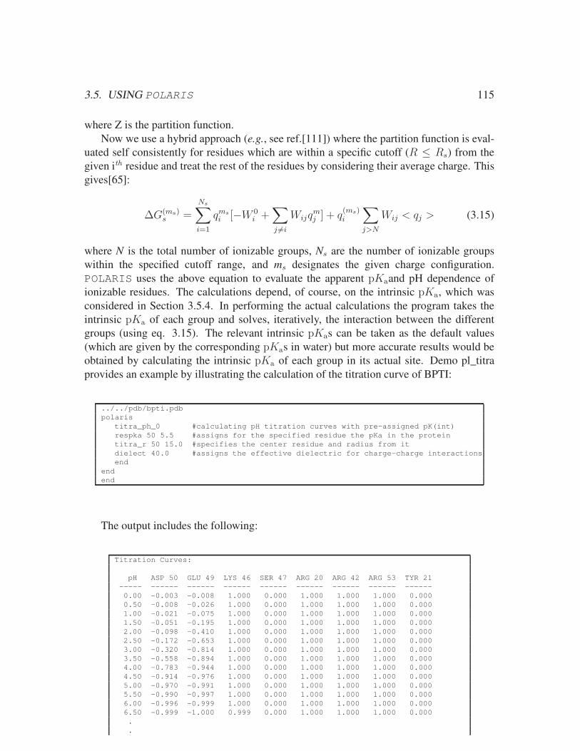
3.5. USING POLARIS 115
where Z is the partition function.Now we use a hybrid approach (e.g., see ref.[111]) where the partition function is eval-
uated self consistently for residues which are within a specific cutoff (R ≤ Rs) from thegiven ith residue and treat the rest of the residues by considering their average charge. Thisgives[65]:
∆G(ms)s =
Ns∑
i=1
qmsi [−W 0i +
∑
j 6=i
Wijqmj ] + q
(ms)i
∑
j>N
Wij < qj > (3.15)
where N is the total number of ionizable groups, Ns are the number of ionizable groupswithin the specified cutoff range, and ms designates the given charge configuration.POLARIS uses the above equation to evaluate the apparent pKaand pH dependence ofionizable residues. The calculations depend, of course, on the intrinsic pKa, which wasconsidered in Section 3.5.4. In performing the actual calculations the program takes theintrinsic pKa of each group and solves, iteratively, the interaction between the differentgroups (using eq. 3.15). The relevant intrinsic pKas can be taken as the default values(which are given by the corresponding pKas in water) but more accurate results would beobtained by calculating the intrinsic pKa of each group in its actual site. Demo pl_titraprovides an example by illustrating the calculation of the titration curve of BPTI:
../../pdb/bpti.pdb
polaris
titra_ph_0 #calculating pH titration curves with pre-assigned pK(int)
respka 50 5.5 #assigns for the specified residue the pKa in the protein
titra_r 50 15.0 #specifies the center residue and radius from it
dielect 40.0 #assigns the effective dielectric for charge-charge interactions
end
end
end
The output includes the following:
Titration Curves:
pH ASP 50 GLU 49 LYS 46 SER 47 ARG 20 ARG 42 ARG 53 TYR 21
----- ------ ------ ------ ------ ------ ------ ------ ------
0.00 -0.003 -0.008 1.000 0.000 1.000 1.000 1.000 0.000
0.50 -0.008 -0.026 1.000 0.000 1.000 1.000 1.000 0.000
1.00 -0.021 -0.075 1.000 0.000 1.000 1.000 1.000 0.000
1.50 -0.051 -0.195 1.000 0.000 1.000 1.000 1.000 0.000
2.00 -0.098 -0.410 1.000 0.000 1.000 1.000 1.000 0.000
2.50 -0.172 -0.653 1.000 0.000 1.000 1.000 1.000 0.000
3.00 -0.320 -0.814 1.000 0.000 1.000 1.000 1.000 0.000
3.50 -0.558 -0.894 1.000 0.000 1.000 1.000 1.000 0.000
4.00 -0.783 -0.944 1.000 0.000 1.000 1.000 1.000 0.000
4.50 -0.914 -0.976 1.000 0.000 1.000 1.000 1.000 0.000
5.00 -0.970 -0.991 1.000 0.000 1.000 1.000 1.000 0.000
5.50 -0.990 -0.997 1.000 0.000 1.000 1.000 1.000 0.000
6.00 -0.996 -0.999 1.000 0.000 1.000 1.000 1.000 0.000
6.50 -0.999 -1.000 0.999 0.000 1.000 1.000 1.000 0.000
.
.

116 CHAPTER 3. SPECIFIC APPLICATIONS AND PRACTICAL ASPECTS
.
Apparent pKa from titration curve:
Res. # pka_i pka_app dpka
------- ------ ------- ------
ASP 50 5.500 3.250 -2.250
GLU 49 4.300 2.250 -2.050
LYS 46 10.400 9.250 -1.150
SER 47 15.000 19.750 4.750
ARG 20 12.500 13.250 0.750
ARG 42 12.500 13.250 0.750
ARG 53 12.500 17.750 5.250
TYR 21 10.460 10.250 -0.210
TYR 23 10.460 13.750 3.290
CYS 5 8.180 7.250 -0.930
CYS 30 8.180 7.750 -0.430
CYS 51 8.180 7.750 -0.430
CYS 55 8.180 7.250 -0.930
Titration demos
The input file used for this example is named titration_3res.inp, and the corresponding pdbfile required for this run is 3_residues.pdb. As for all other examples, please refer to thedemo folder of your current MOLARIS distribution. The input file for this example lookslike this:
3_residues.pdb
polaris
titra_ph_0
crg_method 2
titra_n 1 2 3
monte_r 10
dpka_dielect 80
end
end
end
A few comments, regarding the keywords used in this input: We are using the level ofpolaris/titra_ph_0. The keywords crg_method is used, to choose which method to calculatethe charges should be used. If you use the value of 2, then the method developed by Warsheland Yuk Sham [65], which has been described in the theory, is used. It is suggested thatthe user should use the crg_method of 2, for regular titration runs. The keyword titra_n isused to define the residues in the pdb, which we wish to be titrated. The keyword monte_r
specifies the radius from the center of each titrated residue, where other residues whichare inside this radius can interact with. Finallyl, the keyword dpka_dielect specifies thedielectric constant, required for the electrostatic interactions of each titrated residue.
Using this input file results in an output, where at the end of the file, you can see thetitration curves. An example of those are given in table 3.42 using a dielectric constantof 80, i.e. columns one to four, as well as a dielectric constant of 20, i.e. the remainingcolumns in table 3.42. In figures ?? and ?? these results are illustrated graphically.

3.5. USING POLARIS 117
The apparent pKa calculated by MOLARIS is found at the bottom of the output file too,just after the printed titration curves. Again, for the examples given above using a dielectricconstant of 80, we get:
Apparent pKa from titration curve:
Res. # pka_int pka_app dpka
GLU 2 4.30 3.75 0.55
HIS 3 6.50 6.50 0.00
ARG 1 12.50 12.25 0.25
and for the example using a dielectric constant of 20 we get:
Apparent pKa from titration curve:
Res. # pka_int pka_app dpka
GLU 2 4.30 3.25 -1.05
HIS 3 6.50 6.75 0.25
ARG 1 12.50 12.75 0.25
In this demo run, we observe 3 residues, interacting with each other, with a high di-electric constant (we used the dielectric constant of value 80). That is the main reasonwhy these individual curves, look as if they were titrated individually. However, as shownabove, we may also choose to run the titration example, by having stronger interactionsbetween the titrated residues (that is for the user to decide), then we can alter the value ofthe dielectric constant used.
We now observe that the titration curve of GLU has a major shift, and at lower pH, ithas a higher charge, compared to the one at the same pH, but without the strong influenceof ARG and HIS. The use of different values for the dielectric constant allows the user todevelop a feeling as to how residues interact with each other.
Instead of considering three individual amino acid residues, we may also consider thetitration in a regular protein. For this example, we choose the small SS07D protein for thisrun, (the relaxed version sso_100ps_relax.pdb, or protein 1SSO.pdb from the Protein DataBank). The input file looks like this:
./sso_100ps_relax.pdb
polaris
titra_pH_0
crg_method 2
monte_r 10
dpka_dielect 50
end
end
end
Notice that in this input, we do not specify any particular residue to titrate. When thisis the case, MOLARIS, by default, titrates all possible ionizable residues. Should the userwant to titrate individual residues, one should use the keyword described in the previousexample.
The output of this run, contains all the titration curves from the ionizable residues.

118 CHAPTER 3. SPECIFIC APPLICATIONS AND PRACTICAL ASPECTS
dpka_dielect 80 dpka_dielect 20pH GLU 2 HIS 3 ARG 1 pH GLU 2 HIS 3 ARG 1
0.00 0.000 1.000 1.000 0.00 0.000 1.000 1.0000.50 0.000 1.000 1.000 0.50 0.000 1.000 1.0001.00 -0.001 1.000 1.000 1.00 -0.001 1.000 1.0001.50 -0.002 1.000 1.000 1.50 -0.002 1.000 1.0002.00 -0.005 1.000 1.000 2.00 -0.005 1.000 1.0002.50 -0.016 1.000 1.000 2.50 -0.017 1.000 1.0003.00 -0.050 1.000 1.000 3.00 -0.967 1.000 1.0003.50 -0.157 0.999 1.000 3.50 -0.991 1.000 1.0004.00 -0.453 0.997 1.000 4.00 -0.997 1.000 1.0004.50 -0.806 0.992 1.000 4.50 -0.999 0.999 1.0005.00 -0.941 0.973 1.000 5.00 -1.000 0.998 1.0005.50 -0.982 0.918 1.000 5.50 -1.000 0.994 1.0006.00 -0.994 0.770 1.000 6.00 -1.000 0.980 1.0006.50 -0.998 0.496 1.000 6.50 -1.000 0.923 1.0007.00 -0.999 0.234 1.000 7.00 -1.000 0.285 1.0007.50 -1.000 0.089 1.000 7.50 -1.000 0.088 1.0008.00 -1.000 0.030 1.000 8.00 -1.000 0.030 1.0008.50 -1.000 0.010 1.000 8.50 -1.000 0.010 1.0009.00 -1.000 0.003 1.000 9.00 -1.000 0.003 1.0009.50 -1.000 0.001 0.999 9.50 -1.000 0.001 1.00010.00 -1.000 0.000 0.997 10.00 -1.000 0.000 1.00010.50 -1.000 0.000 0.991 10.50 -1.000 0.000 0.99911.00 -1.000 0.000 0.972 11.00 -1.000 0.000 0.99711.50 -1.000 0.000 0.914 11.50 -1.000 0.000 0.99112.00 -1.000 0.000 0.761 12.00 -1.000 0.000 0.97012.50 -1.000 0.000 0.489 12.50 -1.000 0.000 0.88213.00 -1.000 0.000 0.232 13.00 -1.000 0.000 0.26113.50 -1.000 0.000 0.089 13.50 -1.000 0.000 0.08714.00 -1.000 0.000 0.030 14.00 -1.000 0.000 0.03014.50 -1.000 0.000 0.010 14.50 -1.000 0.000 0.01015.00 -1.000 0.000 0.003 15.00 -1.000 0.000 0.00315.50 -1.000 0.000 0.001 15.50 -1.000 0.000 0.00116.00 -1.000 0.000 0.000 16.00 -1.000 0.000 0.00016.50 -1.000 0.000 0.000 16.50 -1.000 0.000 0.00017.00 -1.000 0.000 0.000 17.00 -1.000 0.000 0.00017.50 -1.000 0.000 0.000 17.50 -1.000 0.000 0.00018.00 -1.000 0.000 0.000 18.00 -1.000 0.000 0.00018.50 -1.000 0.000 0.000 18.50 -1.000 0.000 0.00019.00 -1.000 0.000 0.000 19.00 -1.000 0.000 0.00019.50 -1.000 0.000 0.000 19.50 -1.000 0.000 0.00020.00 -1.000 0.000 0.000 20.00 -1.000 0.000 0.00020.50 -1.000 0.000 0.000 20.50 -1.000 0.000 0.00021.00 -1.000 0.000 0.000 21.00 -1.000 0.000 0.00021.50 -1.000 0.000 0.000 21.50 -1.000 0.000 0.00022.00 -1.000 0.000 0.000 22.00 -1.000 0.000 0.00022.50 -1.000 0.000 0.000 22.50 -1.000 0.000 0.00023.00 -1.000 0.000 0.000 23.00 -1.000 0.000 0.000
Table 3.42: The titration curves given by MOLARIS are printed at the end of each output file. Here, as anexample, two different titrations are given using dielectric constants of 80, i.e. the first four columns, and 20,i.e. in the last four columns.

3.5. USING POLARIS 119
Because the info are too much, MOLARIS prints the titration curves not only in the outputfile, but also in the file named titra_curv.out.
3.5.7 Calculations of ionic strength effects
Electrostatic interactions between macromolecules and their cofactors or substrates can de-pend on the concentration of ions in the surrounding solution. While such effects are usu-ally less important than the interaction between the macromolecule and its cofactor[2], theymight be of interest. The POLARIS program evaluates the effect of the ions in solutions(the ionic strength effect) by solving the Poisson-Boltzmann equation using the approachof Pack and coworkers (e.g., ref. [106]). This is done iteratively for the residual chargeson a cubic grid that surround the solvated macromolecule. The calculations are done ona macroscopic level treating the interactions between the macromolecule charges and thesolution ions (reisual charges) with a dielectric constant ǫ=78.0 and using the same ǫ forthe interaction between the residual charges (you can also change ǫ from this default op-tion value). This approximation is both very effective and quite reliable. The calculationsassume that the Helmholz layer (from which specific ion types are excluded) starts at 3 Åfrom the closest solute atom.
To obtain the ionic strength corrections, just activate the corresponding option inset_opt sublevel keyword in pre_pol level keyword, under POLARIS task key-words in MOLARIS (see ref. manual). This is demonstrated in the demo directorypl_ionic_strength which considers the effect of the ionic strength or the pKaof HIS 64in subtilisin (see [13]). The demo input file looks like:
../pdb/sub.pdb
polaris
pre_pol
ionres 32
set_opt
ionic 1 1.0 #ionic strength effect is calculated
end #and the value for ionic concentration
pka_pdld
reg1_res 64
config 0 2
md_parm_r
nsteps 1000
end
md_parm_w
nsteps 300
end
md_parm_p
nsteps 1000
end
end
end
end
The relevant part of the output will appear in the pKa_pdld.out file and will look like:
----------------------------------------
Summary of pKa for the different configs
----------------------------------------
PDLD SEMI-MACROSCOPIC ESTIMATE FOR pKa
......................................

120 CHAPTER 3. SPECIFIC APPLICATIONS AND PRACTICAL ASPECTS
effective dielectric 2 4 6 8 20 40 80
epsilon_p(e_p)
pKa_intr for str. 1 1.65 4.14 4.97 5.39 5.95 6.29 6.47
pKa_intr for str. 2 3.38 5.01 5.55 5.83 6.04 6.34 6.49
----------------------------------------------------------------------------
aver pKa_int 2.51 4.58 5.26 5.61 5.99 6.32 6.48
estimated apparent pKa 5.70
average ddE_ionic = 0.581 ion concentration = 1.0M
3.5.8 Redox Potentials of Proteins
Much has been learned about the overall properties that determine the redox potential,which provides the driving force for electron transfer reactions. However, it is still not clearhow all the key residues, which are in close proximity to the heme group in cytochrome C,contribute to the observed redox value.
Recent advances in site-specific mutagenesis provide a powerful tool to dissect the con-tributions to the observed redox potential that arise from any specific residue. Apparentlythe redox potential is controlled by the interrelated contributions from the entire surround-ing of the heme moiety. Changes in one residue can be accompanied by changes in theprotein and water environment. This effect, which can be formally considered as a di-electric effect, might include significant structural changes of the protein and/or local re-arrangement of a few water molecules at the site of the mutation. Thus, a quantitativeunderstanding of the effect of a point mutation requires some type of structure-redox cor-relation. Such a correlation requires computational analysis of the relationship between theredox energetics and the heme environment in addition to structural studies based on X-raycrystallography.
Such an approach is provided by the redox_pdld feature of POLARIS. The method hasbeen found sufficiently reliable to reproduce the observed effect of different mutations andhas provided a more comprehensive understanding of structure and function relationshipsof redox proteins. For example, the method has been validated in correlations linking aminoacid sequence changes to the redox potential of electron transfer reactions in proteins usingthe Asn52->Ile mutation in cytochrome c as a test case. Other examples are provided bycalculations of the energetics of photosynthetic proteins (see ref.[112]) and studies of iron-sulfur proteins (see refs.[113, 114]). Practical instructions for redox calculations using thePOLARIS program are given below.
The redox potential is the potential required to take the given cofactor from the state ofhigher absolute charge (say state A) to the state of lower absolute charge (say state B) inthe presence of Region II and water.
As in the case of pKa calculations, we use the trick of eq. (3.8) where the redoxpotential of the given group in water is the reference for the evaluation of the absoluteredox potential of this group in its actual protein site:
∆ξp1/2 =−∆∆Gw→p
sol
F+∆ξw1/2 (3.16)

3.5. USING POLARIS 121
where F is the Faraday constant, ∆ξ1/2 is the midpoint redox potential of the givenmolecule, while p and w designate protein and solution, respectively. If the experimen-tal value of the redox potential in pure water is not known the user should type 0.0. Tocalculate the redox potential, you can either type redox_pdld at the prompt ‘command>‘.Calculations of redox potential involve an average over several protein configurations andthey reflect, correctly, the effect of the protein reorganization energy.
The average PDLD/S estimate of the free energy and redox potential is obtained asfollows. First we evaluate the PDLD/S-LRA free energy for the oxidation procedure (aminus sign will make it a reduction procedure)
∆∆Gw→predox = −∆∆Gw→p
redox(D → D+) (3.17)
= −1
2m
∑
m
([∆Gw→ppdld/s(D → D+)D+ +∆Gw→p
pdld/s(D → D+)D]
(3.18)
where m is the number of configurations generated by MD simulations, D and D+ arethe reduced and oxidized donor (heme+ligands), respectively and ( )D+ designates thecorresponding configuration generated during an MD average over D. The ∆∆G is alreadytreated as the rigorous free energies (within the LRA approximation) while the ∆∆Gpdld/s
is the PDLD/S effective potential. (See ref. [115]).To familiarize yourself with redox calculations it is useful to run the following exam-
ple for the blue copper protein with POLARIS com file for redox - bc_redox.inp in thepl_redox_pdld directory of the demo. The input looks as follows:
../pdb/pc.pdb
analyze
allres
resatom 100
resatom 84
resatom 87
resatom 37
resatom 92
end
polaris
redox_pdld
reg1_res 100 84 87 37 92 #Coordinates and charges of Reg I
ab_crg 530 0.000 0.000
ab_crg 531 0.000 0.000
ab_crg 532 0.000 0.000
ab_crg 533 0.000 0.000
ab_crg 534 0.000 0.000
ab_crg 535 0.000 0.000
ab_crg 536 0.000 0.000
ab_crg 537 0.035 0.035
ab_crg 538 -0.227 -0.302
ab_crg 539 0.187 0.187
.
.
redox_w 500 #value of E(1/2) in water
config 1 5
.
.
.
end

122 CHAPTER 3. SPECIFIC APPLICATIONS AND PRACTICAL ASPECTS
The output file (redox_pdld.out) contains at its end the following results:
***************************************************PDLD SEMI-MACROSCOPIC ESTIMATE FOR REDOX IN PROTEIN
***************************************************
effective dielectric 2 4 6 8 20
(epsilon-p)
redox for structure 1: 662.52 581.25 554.16 540.61 512.93
redox for structure 2: 664.33 582.23 554.86 541.18 514.73
redox for structure 3: 658.27 579.16 552.79 539.60 514.22
redox for structure 4: 605.21 552.65 535.13 526.37 508.65
redox for structure 5: 599.73 549.84 533.21 524.90 509.92
-----------------------
average (mV) : 638.01 569.02 546.03 534.53 512.09
One of the best demonstrations of the usefulness of POLARIS is provided by the exten-sive study of redox property of iron sulfur proteins (see ref. [114]). The user can examinethis important class of proteins by running the demo com file in redox/Fe_S.cluster.
3.5.9 Calculations of binding free energies
The development of a reliable method for the evaluation of absolute binding free energiesof ligand protein complexes is of significant practical and fundamental interest. An effec-tive method should provide a guide for rational drug design and help in providing a deeperunderstanding of structure function correlation in proteins. Reliable estimates of bindingfree energies should help in identifying and refining lead compounds in computer-aideddrug design. Different strategies can be used in studies of absolute binding energies. Thisinclude formally rigorous approaches such as the Free Energy Perturbation (FEP) method,which is usually restricted to mutations of small parts of the ligand and the all-atom Lin-ear Response Approximation (LRA) and its variants, which allows one to calculate theabsolute binding energy of relatively large ligands. More approximated and significantlyfaster approaches, which frequently focus on electrostatic energies, are also quite effective.These include the scaled Protein Dipoles Langevin Dipoles (PDLD/S) method and the LRAversion of this approach (PDLD/S-LRA) as well as other approaches.
POLARIS provides the unique opportunity of evaluating binding free energy by themost effective approaches including the PDLD/S-LRA, LRA and LIE. It also provides theability (which is not common to other programs) of comparing the different approachesand understanding their interrelations. The main points are clearly discussed in [59]
In order to understand the philosophy behind our calculations of binding free energiesit is useful to start from the general binding cycle depicted in Fig. 3.13. In the upper cycle

3.5. USING POLARIS 123
∆Gbind,l
∆Gbind,l’’
∆Gbind,l’
l’’l’’
l’l’
ll
∆Gwl’’-->l’∆Gpl’’-->l’
∆Gpelec,l ∆Gwelec,l
(a)
(c)
(f) (e)
(d)
(b)
Figure 3.13: A thermodynamic cycle that describes the binding of a ligand to a protein and provides a cleardefinition of the LRA and LIE approximations. The electrostatic contributions to the binding free energy,∆Gwelec,ℓ and ∆G
pelec,ℓ′ can be calculated reliably by using the LRA method for the process of “uncharging”
the residual charges of the polar ligand to zero in water (a → b) and in protein (c → d), respectively. Theestimation of the ∆Gbind,ℓ′ term considers the lower cycle (b → e → f → c) and can be carried out by ashrinking process describe in the text.

124 CHAPTER 3. SPECIFIC APPLICATIONS AND PRACTICAL ASPECTS
(a→ b→ c→ d), we start by taking the ligand (ℓ) in water and “uncharging” it by settingall the residual charges to zero. Next we take the non-polar ligand (ℓ′) and bind it to theprotein. Finally we recharge (ℓ′) in the protein active site. The binding free energy is nowgiven by:
∆Gbind,ℓ = ∆Ga→b +∆Gb→c +∆Gc→d
= −∆Gwelec,ℓ +∆Gbind,ℓ′ +∆Gp
elec,ℓ (3.19)
where ∆Gbind,ℓ′ is the free energy of binding the non-polar ligand to the protein, while∆Gw
elec,ℓ and ∆Gpelec,ℓ are the electrostatic free energies associated with charging the ligand
in water (w) and in protein (p), respectively.Below we describe several strategies for evaluating the three terms of eq. 3.19.
PDLD/S-LRA calculations of binding free energies
The most crucial trick in the cycle of Fig. (3.13) is the formulation of the binding freeenergy as a sum of well defined electrostatic terms plus a more elusive term (∆Gbind,l′) thatrepresents the binding of the uncharged ligand [6]. The electrostatic terms lend themselvesto a convinient evaluation by the LRA and PDLD/S-LRA method; In particular, we canuse the thermodynamic cycle of Fig. (3.14), which is in fact the PDLD/S equivalent of thecycle of Fig. (2.12) and the upper cycle of our original LRA study [6]. Now the relevantPDLD/S-LRA electrostatic contributions are given by
∆Gelecbind,ℓ = ∆Gelec
p,ℓ −∆Gelecw,ℓ +∆Gelec
bind,ℓ′ (3.20)
In evaluating the first two terms of Eq. 3.20, we start by considering a single configu-ration (s) for the protein-ligand complex and a single configuration (s’) for the dissociatedcomplex. The effective electrostatic potential for both the a → b and c → d steps areevaluated by the PDLD/S approach, where the results of the microscopic PDLD model arescaled by considering the external cycles c → c′ → d′ → d and a → a′ → b′ → b. Thesecycles involve a change of the dielectric constant of the solvent around the protein from thatof water, εw, to the value of the so-called protein dielectric, εin, (this parameter representsthe contributions which are not treated explicitly[74]). The overall potentials for the twocycles are given by
(∆Gpelec,ℓ)s = Up
elec,ℓ = (3.21)(
(∆Gℓ+psol −∆Gℓ′+p
sol )
(
1
εin−
1
εw
)
+∆Gℓsol
(
1−1
εw
)
+U ℓqµ
εin+U ℓintra
εin
)
s
(∆Gwelec,ℓ)s′ = Uw
elec,ℓ = (3.22)(
∆Gℓsol
(
1
εin−
1
εw
)
+∆Gℓsol
(
1−1
εin
)
+U ℓintra
εin
)
s′

3.5. USING POLARIS 125
Figure 3.14: A thermodynamic cycle for calculating binding energy using the PDLD/S method. The innerbinding cycle (a → b → c → d) is equivalent to that of Fig. (3.13) and to a part of the cycle used by Leeet al.[6] The electrostatic terms associated with a → b and c → d are evaluated by the external cycles inthe figure (a → a′ → b′ → b and c → c′ → d′ → d) and are evaluated by using Eqs. 3.22 with ǫin = 4.The free energy ∆Gbind,ℓ′ , and the other contributions of ∆Gbind,ℓ′ , are evaluated by Eq. 3.26 using anapproximation to the b → e → f → c cycle.
where we use U rather than U to designate the fact that U is an effective potential ratherthan the fully microscopic potential of the previous sections. ∆Gsol denotes the electro-static contribution to the solvation free energy of the indicated group in water (e.g., ∆Gℓ+p
sol
denotes the solvation of the protein-ligand complex in water). To be more precise, ∆Gsol
should be scaled by 1/(1 − 1/εw) but this small correction is neglected here. The valuesof the ∆Gsol’s are evaluated by the Langevin dipole solvent model. U ℓ
qµ is the electro-static interaction between the charges of the ligand and the protein dipoles in vacuum (thisis a standard PDLD notation). In the present case U ℓ′
qµ = 0. U ℓintra is the intramolecu-
lar electrostatic interaction of the ligand. Now the PDLD/S results obtained with a singleprotein-ligand configuration cannot capture properly the effect of the protein reorganiza-tion (see discussion in Sham et al.[65]) and a more consistent treatment should involve theuse of the LRA or related approaches (e.g., [6, 65]). This approach provides a reasonableapproximation for the corresponding electrostatic free energies by using the equivalent ofEq. 2.21:
∆Gxelec,ℓ =
1
2
[
〈Uxelec,ℓ〉ℓ′ + 〈Ux
elec,ℓ〉ℓ]
(3.23)
where x is p or w. The effective potential U is defined in Eq. 3.22, 〈〉ℓ and 〈〉ℓ′ designatean MD average over the coordinates of the ligand-complex in their polar and non-polarforms. It is important to realize that the average of Eq. 3.23 is always done where bothcontributions to the relevant Uelec are evaluated at the same configurations. That is, thePDLD/S energies of the polar and non-polar states are evaluated at each averaging step byusing the same structure. However, we generate two set of structures one from MD runs

126 CHAPTER 3. SPECIFIC APPLICATIONS AND PRACTICAL ASPECTS
on the polar state and one from MD runs on the non-polar state. This is basically the sameapproach used in the microscopic LRA but now with the effective potential Uelec.
Next we have to evaluate the binding free energy of the non-polar ligand, ∆Gbind,ℓ′ ,of the lower cycle of Fig. (3.14), where we mutate ℓ′ to a shrinked ligand ℓ′′. This muta-tion procedure gives more stable results than those obtained by our previous strategy thatinvolved the direct b → c step, which requires a direct evaluation of the solvation en-ergy of the isolated protein. In implementing step f → c, it is not so practical to use theLRA approach. The problem is that running trajectories with the potential of ℓ′′ may leadto exponentially large contributions from the vdW energies of ℓ′. Thus, we approximate∆Gℓ′′→ℓ′ by
∆Gp,elecℓ′′→ℓ′ ≈ 〈Up
elec,ℓ′〉ℓ′ − 〈Upelec,ℓ′′〉ℓ′′ = 〈Up
elec,ℓ′′→ℓ′〉ℓ′ (3.24)
where we average the PDLD contributions for ℓ′ over trajectories obtained with the poten-tial of ℓ′ and average the contributions from ℓ′′ over trajectories obtained with the potentialof ℓ′′. The effect of the protein reorganization upon change from ℓ′′ to ℓ′ is neglected, sinceit is assumed that the major part of the protein relaxation occurs in the charging step ℓ→ ℓ′
(see however, ref. [34]). One may wonder why our electrostatic contribution is differentthan zero since the protein-ligand electrostatic interaction is zero and thus the correspond-ing FEP or LRA contribution will be zero. However, in an actual FEP procedure, thatconsiders the ℓ′ → ℓ′′ transformation, the non-zero van der Waals contribution dependson the reorganization of the system. This contribution reflects the change in protein-water(rather than protein-ligand) electrostatic interaction as a result of water penetration and thiseffect is approximated by our ∆Gp,elec
ℓ′′→ℓ′ . The same approximation used in the evaluation of∆Gp,elec
ℓ′′→ℓ′ is used for the vdW and hydrophobic term giving
∆Gp,vdWℓ′′→ℓ′ −∆Gw,vdW
ℓ′′→ℓ′ +∆Gp,hydℓ′′→ℓ′ −∆Gw,hyd
ℓ′′→ℓ′ =
= 〈UpvdW,ℓ′〉ℓ′ − 〈Up
vdW,ℓ′′〉ℓ′′ + 〈Uphyd,ℓ′〉ℓ′ − 〈Up
hyd,ℓ′′〉ℓ′′ (3.25)
where UvdW , designates the PDLD vdW interaction and Uhyd designates the field-dependentPDLD hydrophobic energy.[13] Now our final expression for ∆Gbind,ℓ′ , is
∆Gbind,ℓ′ = ∆Gpℓ′′→ℓ′ −∆Gw
ℓ′′→ℓ′
= ∆Gp,elecℓ′′→ℓ′ +∆Gp,vdW
ℓ′′→ℓ′ +∆Gp,hydℓ′′→ℓ′ −
− ∆Gw,vdWℓ′′→ℓ′ −∆Gw,hyd
ℓ′′→ℓ′ − T (∆∆S ′ℓ′)
w→p
= ∆GPDLD/Sbind,ℓ′ − T (∆∆S ′
ℓ′)w→p (3.26)
The term (∆∆S ′ℓ′)
w→p represents the loss of configurational entropy upon moving ℓ′ fromwater to the protein active site rather than that associated with e → f step. This is, ofcourse, not the case in FEP studies where the entropic contribution is obtained in the ℓ′ →ℓ′′ steps. Finally, we scale the contributions to ∆Gbind,ℓ′ , by θ and use
∆Gbind,ℓ′ = θ{
∆GPDLD/Sbind,ℓ′ − γ[T (∆∆S ′
ℓ′)′]}
(3.27)
The results of our calculations depend, of course, on the ionization state of differentprotein residues and thus on the pH of the surrounding solvent. This pH effect can be

3.5. USING POLARIS 127
calculated by our PDLD/S-LRA approach. In this approach, we calculate first the intrinsicpKa of each ionizable residue and then evaluate the effective interaction between theseresidues by a hybrid approach (for details see [65]). The calculations include the ligand (ℓ)in its polar state. At any rate, we can write (this is eq. 12 from [59])
∆Gelec/PDLD/S−LRAbind =
1
2
{
[
〈Upelec,ℓ〉ℓ′ + 〈Up
elec,ℓ〉ℓ′]
−[
〈Uwelec,ℓ〉ℓ′ + 〈Uw
elec,ℓ〉ℓ′]
}
(3.28)
and with the non electrostatic term we get:
∆GPDLD/S−LRA = ∆Gelec/PDLD/S−LRA +∆Gbind,ℓ′ (3.29)
PDLD/S-LRA/β
Instead of calculating the electrostatic and non-electrostatic contribution to the bindingfree energy with the PDLD/S-LRA method, one may also approximate the free energy ofbinding using (eq. (13) from [59]):
∆GPDLD/S−LRA/βbind = ∆G
elec/PDLD/S−LRAbind + β(〈Up
vdw,l〉l − 〈Uwvdw,l〉l) (3.30)
where ∆Gelec/PDLD/S−LRAbind is calculated according to the equivalent of equation 3.23
- just as it is done in the standard PDLD/S-LRA approach descibed above - and the non-electrostatic van der Waals term is scaled, using multiple linear regression analysis de-scribed in the next section, to fit the experimental binding free energy. This approach, re-ferred to as the PDLD/S-LRA/β method [59], together with LIE and LRA-type approacheswere successfully applied to calculate the free energies of binding of series of inhibitorscomplexed to various proteins [59]. As an example we illustrate the use of the PDLDroutines of MOLARIS to calculate the free energies of binding of inhibitors complexed toHIV Protease. All necessary input files can be found in the directory pdld_bind of yourMOLARIS distribution. The input file bind_1.inp looks like this:
relax.pdb keepnoh #load the PDB file
y
enzymix # enter enzymix for initial relaxation
relax
md_parm
np 5000
ss 0.001
temp 30
end
end
end
polaris #enter the POLARIS module
pre_pol #set some parameters for PDLD
ionres 25 #ionize ASP25 Achain
end
bind_pdld #enter he PDLD binding routines
reg1_res 199 #identify region I
config 0 4 #configurations to be done
md_parm_r #relaxation dynamics
np 45000
stepsize 0.001

128 CHAPTER 3. SPECIFIC APPLICATIONS AND PRACTICAL ASPECTS
constraint_1 3.0
constraint_2 0.01
induce 2
indforce 1
end
md_parm_w #dynamics in water
stepsize 0.001
np 1200
constraint_1 3.0
induce 2
indforce 1
end
md_parm_p #dynamics in the protein
np 1200
stepsize 0.001
constraint_1 3.0
constraint_2 0.01
induce 2
indforce 1
end
end
end
end
end
In fact, using this input results in various output files generated by MOLARIS. For thePDLD/S-LRA/β approach the most important file produced is bind_pdld_s_lra_beta.out,as it contains all the contributions necessary to calculate the free energy of binding. How-ever, also the file md_lie.out and md_lra.out are being generated by MOLARIS offering thepossibility of LRA or LIE analysis.
Apart for most PDLD-related energy terms that have already been covered in thePOLARIS section, the calculated free energies of binding can be found at the very bot-tom of the file bind_pdld_s_lra_beta.out:
calculated PDLD/S-LRA/Beta binding free enregy
.....................................
dG_bind = c1*ddV_elec (PDLD)+ c2*ddV_nonelec (from MD)
= ddG_elec + ddG_nonelec
c1 ddG_elec c2 ddG_ne dG_bind
------------------------------------------------------------------------
PDLD/S-LRA/Beta estimate 0.50 -2.66 0.25 -7.75 -10.41
------------------------------------------------------------------------
Thus, our calculated absolute free energy of binding using a scaling factor of 0.25 forthe non-electrostatic contribution stands at -10.41 as opposed to the experimental result of-10.40 kcal/mol [59].
Linear regression (QSAR) treatment of the PDLD/S-LRA results
As we noted [116] the predictive power of the PDLD/S approach can be increased byintroducing an ad-hoc linear regression approach which involve scaling of the differentfree energy terms. That is, in analyzing the binding of different ligands to a given proteinwe may write:
∆Gbind = C1(∆Gelecp,ℓ −∆Gelec
w,ℓ ) + C2∆GPDLD/Sbind,ℓ′ − C3[T (∆∆S ′
ℓ′)′] (3.31)

3.5. USING POLARIS 129
Here the Cis are correlation coefficients. The correlation terms can be determined byperforming the calculations on several ligands and using a standard linear regression treat-ment (which can be found in standard softwares such as Excel and Mathematica) and mini-mizing the difference between the calculated and the observed. With optimized correlationcoefficients you can study new ligands. Note that this approach is not much different thanstandard QSAR treatments except that now we deal with more quantitative energy contri-butions.
LRA, LIE and the LRA/β approach
POLARIS allows you to evaluate binding free energies by the more rigorous but muchmore expensive all-atom LRA [8, 34] and LIE [117] approaches. These two closely relatedapproaches (see discussion in ref. [34]) involve the thermodynamic cycle of Fig. 3.13whose binding energy is given by Eq. 3.19. The electrostatic contributions in this equationcan be evaluated by the microscopic LRA method using:
∆Gwelec,ℓ =
1
2(< ∆Uw
elec,ℓ′→ℓ >ℓ + < ∆Uwelec,ℓ′→ℓ >ℓ′) (3.32)
=1
2(< ∆Uw
elec,ℓ >ℓ + < ∆Uwelec,ℓ >ℓ′)
∆Gpelec,ℓ =
1
2(< ∆Up
elec,ℓ′→ℓ >ℓ + < ∆Upelec,ℓ′→ℓ >ℓ′)
=1
2(< ∆Up
elec,ℓ >ℓ + < ∆Upelec,ℓ >ℓ′)
where Uelec,ℓ designates the electrostatic interactions between the ligand and its surround-ing. Here ∆Uelec,ℓ′→ℓ = Uelec,ℓ−Uelec,ℓ′ and we make use of the fact that Uelec,ℓ′ = 0. Nowwe obtain from Eqs. 3.19 and 3.32:
∆GLRAbind,ℓ =
1
2
[
(< Upelec,ℓ >ℓ + < Up
elec,ℓ >ℓ′)− (< Uwelec,ℓ >ℓ + < Uw
elec,ℓ >ℓ′)]
+∆Gbind,ℓ′ = (∆∆Gw→pelec,ℓ)
LRA +∆Gbind,ℓ′ (3.33)
This is eq. (6) in [59] (where it has asmall typo of ’-’ instead of ’+’). ∆Gbind,ℓ can beobtained by the lower cycle of Fig 3.13 (b → e → f → c). In this cycle we shrink thenon-polar ligand, ℓ′, to nothing, ℓ′′, in water, then bind the zero size ligand to the protein,and finally grow it back to its original size in the protein. This gives:
∆Gbind,ℓ′ = ∆Gpℓ′′→ℓ′ −∆Gw
ℓ′′→ℓ′ +∆Gbind,ℓ′′ (3.34)
The terms ∆Gwl′′→l′ and ∆Gp
l′′→l′ can be evaluated, at least in principle, by FEP approachesor related treatments (see ref. [34]). In most cases we prefer to use the PDLD/S estimate ofEq. 3.27. Several approximations can be applied to Eq. 3.33. One useful approach involvesthe neglect of < Uelec,l >l′ . This is justified for a charging process in water where the waterdipoles are oriented randomly around the non-polar state and the solvationenergy is givenby 1/2 < Uw
elec,l >l′[2]. In proteins, however, it is not fully justified to neglect < Upelec,l >l′ ,
130 CHAPTER 3. SPECIFIC APPLICATIONS AND PRACTICAL ASPECTS
since the protein environment can remain preoriented even in the presence of the non-polarligand (see ref. [34]). At any rate one may try to use the approximation:
∆Gbind,ℓ∼=
1
2(< Up
elec,ℓ >ℓ −Uwelec,ℓ >ℓ) + ∆Gbind,ℓ′ (3.35)
This expression leads to the so called LIE approximation [117], which expresses thebinding energy as (eq. (7) in [59]):
∆GLIEbind,ℓ = α(< Up
elec,ℓ >ℓ − < Uwelec,ℓ >ℓ) + β(< Up
vdw,ℓ >ℓ − < Uwvdw,ℓ >ℓ) (3.36)
where α and β are scaling constants while Uelecℓ designates the electrostatic interactionbetween the ligand and its surrounding. The rational for this has been provided in ref.[117] by a some what less rigorous way than that used in deriving Eq. 3.33. That is,qvist et al. [117] considered the electrostatic part of the binding process as a transitionfrom a state (state A) with the isolated ligand in the gas phase and a protein with a readymade cavity (in the shape of the ligand) to a state (state B) where the ligand is boundto the protein. The electrostatic contribution of this process was estimated by the LRAapproximation. Although such a process is conceptually valid, it is difficult to treat thepotential UA in actual calculations without introducing an actual non-polar ligand (or arelated constraint) in the cavity. This problem was removed in a recent work[118], whichessentially used the cycle introduced earlier by Lee et. al.[6] (the a → b → c → d cycleof Fig. 3.13 of the present work and the upper cycle of Fig. 1 of ref. [6]) to jusify the LIEapproach. The cycle of ref. [118], however, keeps the intramolecular interactions withinthe ligand, upon annihilating the ligand-protein electrostatic interaction, while Lee et. al.also annihilated the intramolecular interactions within the ligand. Now the LIE approachevaluates the ∆∆Gbind,ℓ′ term using the vdw interactions of the polar rather than non-polarligand (this is needed since the LIE does not involve simulations of the non-polar ligand).
As stated above our LRA approximation of Eq. 3.33 combines the approach used byLee et. al.[6] in the first implementation of the LRA treatment in calculations of bindingfree energies with a microscopic estimate of the entropic term. This approach retains therigorous LRA terms of Eq. 3.33 but approximates ∆Gbind,ℓ′ by the PDLD/S contribution,but we also use an approach called LRAβ where ∆Gbind,ℓ′ is estimated in the same way asin the LIE approach by the ad-hoc scaling of Vvdw. In this case we use (eq. (8) in [59]:
∆GLRA/βbind =
1
2
[
(< Upelec,ℓ >ℓ − < Uw
elec,ℓ >ℓ) + (< Upelec,ℓ >ℓ′ − < Uw
elec,ℓ >ℓ′)]
+β(< UpvdW,ℓ >ℓ − < Uw
vdW,ℓ >ℓ) (3.37)
The all-atom LRA, LRA’ and LIE calculations are done automatically during thePDLD/S calculations and the corresponding results are given in the files called lra.out,md_lra.out and md_lie.out.
Group contributions to binding
The PDLD/S approach can also be useful in estimating the electrostatic contribution ofeach protein residue to the binding process. Theses contributions can provide a ’road map’

3.5. USING POLARIS 131
for locating ’hot’ residues whose mutations are likely to change the functional propertiesof the protein [119]. The electrostatic contribution of the ith residue [120] is defined as thechange in the electrostatic contribution to the binding upon mutation of the ith residue to aGly or upon turning off the residual charges of the ith residue.
(∆∆G(i)bind) =<
U(i)qµ
εin> + < ∆Gℓ+p
sol −∆Gpsol >
(i) (1
εin−
1
εw) (3.38)
where < >(i) is the contribution to indicated term from the ith residue. Since the effect ofthe solvent around the protein is expected to be small when a nonionized residue becomesa non polar residue, we can approximate Eq. 3.38 by:
(∆∆G(i)bind)unionized =<
U(i)qµ
εin> (3.39)
For an ionized residue it has been found [120] that the best result is obtained with thesimplified expression:
(∆∆G(i)bind)ionized =<
U(i)qµ
εeff> (3.40)
where εeff is the effective dielectric of Eq. 3.13.This evaluation of the group contributions is done automatically during the PDLD/S
calculation of the absolute binding energy. The results are summarized at the beginning ofthe bind_pdlds.out file along with the corresponding average distance between the residueto the center of the bound ligand.
3.5.10 Ion channels
The POLARIS program provides a powerful way of studying ion channels (particularlywhen coupled with an automatic generation of channel configurations by the programENZYMIX). The program can provide the energy profile for the ion penetration througha channel within the membrane taking into account the different electrostatic contributionsfrom the channel’s permanent dipoles, the water molecules inside and outside the channeland the membrane induced dipoles. Extensive studies are described in refs. [121, 122]. Anexample for Na+ in a Gramacidin channel is given in: [123] old POLARIS com file for
channel - channel.com
3.5.11 Calculating electric fields
If the keyword field is activated in the set_opt sublevel keyword in pre_pol levelkeyword, under POLARIS task keywords in MOLARIS (see ref. manual) (it has a defaultvalue of 0), then the program will create a file called field.dat. This file contains thecoordinates of all of the protein atoms and Langevin dipoles in the system and the electricfield vector at each point. This field is due to the state A charges, the region 2 charges andthe Langevin dipoles. The file is formatted with the following format of each record:
• Format: [5X,3F8.3,5X,3F8.3,5X,I5] - first three numbers are the coordinates of thepoint and the last three real numbers are the electric field vector, the final integer is 1 forregion one atoms, 2 for region two atoms and 3 for Langevin dipoles.

132 CHAPTER 3. SPECIFIC APPLICATIONS AND PRACTICAL ASPECTS
The coordinates are in Å and the electric field is in units of kcal/(electron charge x Å).
The file field.dat can be plotted by the program MOLARIS or by one of the users ownprograms. If you do not have MOLARIS one way to plot the field is to generate atom pairsfrom each field vector, to incorporate these pairs in the PDB file and then to plot themassigning, say, blue and red colors, respectively, to the first and second atom in each pair.
3.5.12 LD calculations using Chemsol
The program ChemSol is designed for the calculations of solvation free energies by usinga Langevin Dipoles (LD) model of the solvent. The implementation, parameterizationfor aqueous solution, and some applications of the model are described in detail in refs.Florián, 1997 and Florián, 1999. To obtain a copy of these manuscripts send an e-mail toJan Florián ([email protected]). Also, you can go to our web page http://laetro.usc.edu for contact information and for running ChemSol on-line free of charge.
Copies of the program ChemSol can be downloaded free of charge from anonymous ftpat: ftp.usc.edu, directory pub/warshel/cs.
3.6 Using the CG model
The CG model described in section 2.3 can be used in many applications. Some are con-sidered below, as well as instructions and demos for the CG calculations.
3.6.1 Trimming
We start this practical part by showing how you can use a small protein (such as PDB ID1SSO) as an input, and create a trimmed, i.e. coarse-grained, representation of it. The inputfile looks like this:
./sso_100ps_relax.pdb fold2 0 0 0 0 # PDB input file
analyze
allres
makepdb
file_nm sso_simp.pdb
residue all
end
end # End of analyze
end # End of Molaris
In the following examples, as was done in previous sections, the bold characters denotea keyword, and with italic we denote a MOLARIS "level". For example, from the inputgiven above, allres is a keyword. On the other hand, analyze and makepdb are MOLARISlevels. The text followed by the input file - "fold2 0 0 0 0" in the example above - consistsof the arguments to trim the amino acid residues accordingly.
The analyze level of the input file will produce a new pdb file from the coordinates of
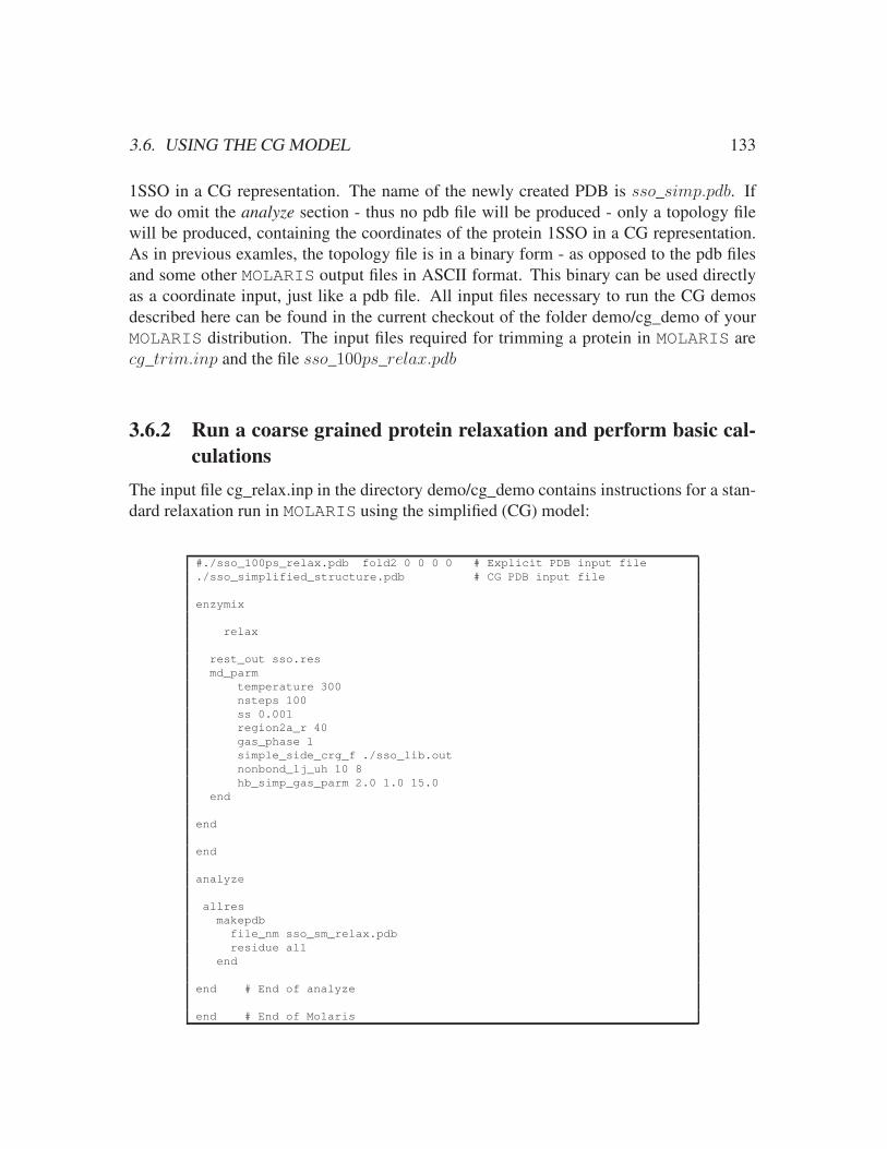
3.6. USING THE CG MODEL 133
1SSO in a CG representation. The name of the newly created PDB is sso_simp.pdb. Ifwe do omit the analyze section - thus no pdb file will be produced - only a topology filewill be produced, containing the coordinates of the protein 1SSO in a CG representation.As in previous examles, the topology file is in a binary form - as opposed to the pdb filesand some other MOLARIS output files in ASCII format. This binary can be used directlyas a coordinate input, just like a pdb file. All input files necessary to run the CG demosdescribed here can be found in the current checkout of the folder demo/cg_demo of yourMOLARIS distribution. The input files required for trimming a protein in MOLARIS arecg_trim.inp and the file sso_100ps_relax.pdb
3.6.2 Run a coarse grained protein relaxation and perform basic cal-
culations
The input file cg_relax.inp in the directory demo/cg_demo contains instructions for a stan-dard relaxation run in MOLARIS using the simplified (CG) model:
#./sso_100ps_relax.pdb fold2 0 0 0 0 # Explicit PDB input file
./sso_simplified_structure.pdb # CG PDB input file
enzymix
relax
rest_out sso.res
md_parm
temperature 300
nsteps 100
ss 0.001
region2a_r 40
gas_phase 1
simple_side_crg_f ./sso_lib.out
nonbond_lj_uh 10 8
hb_simp_gas_parm 2.0 1.0 15.0
end
end
end
analyze
allres
makepdb
file_nm sso_sm_relax.pdb
residue all
end
end # End of analyze
end # End of Molaris
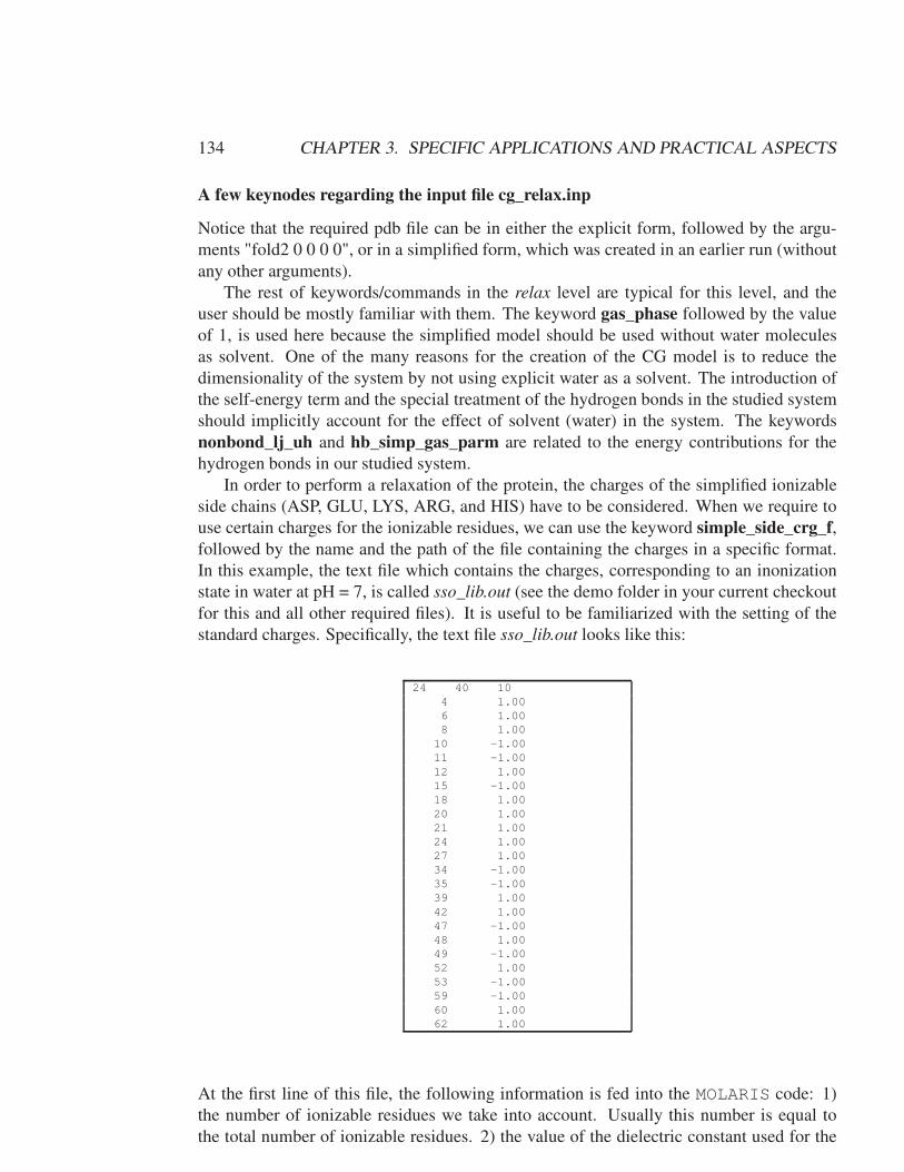
134 CHAPTER 3. SPECIFIC APPLICATIONS AND PRACTICAL ASPECTS
A few keynodes regarding the input file cg_relax.inp
Notice that the required pdb file can be in either the explicit form, followed by the argu-ments "fold2 0 0 0 0", or in a simplified form, which was created in an earlier run (withoutany other arguments).
The rest of keywords/commands in the relax level are typical for this level, and theuser should be mostly familiar with them. The keyword gas_phase followed by the valueof 1, is used here because the simplified model should be used without water moleculesas solvent. One of the many reasons for the creation of the CG model is to reduce thedimensionality of the system by not using explicit water as a solvent. The introduction ofthe self-energy term and the special treatment of the hydrogen bonds in the studied systemshould implicitly account for the effect of solvent (water) in the system. The keywordsnonbond_lj_uh and hb_simp_gas_parm are related to the energy contributions for thehydrogen bonds in our studied system.
In order to perform a relaxation of the protein, the charges of the simplified ionizableside chains (ASP, GLU, LYS, ARG, and HIS) have to be considered. When we require touse certain charges for the ionizable residues, we can use the keyword simple_side_crg_f,followed by the name and the path of the file containing the charges in a specific format.In this example, the text file which contains the charges, corresponding to an inonizationstate in water at pH = 7, is called sso_lib.out (see the demo folder in your current checkoutfor this and all other required files). It is useful to be familiarized with the setting of thestandard charges. Specifically, the text file sso_lib.out looks like this:
24 40 10
4 1.00
6 1.00
8 1.00
10 -1.00
11 -1.00
12 1.00
15 -1.00
18 1.00
20 1.00
21 1.00
24 1.00
27 1.00
34 -1.00
35 -1.00
39 1.00
42 1.00
47 -1.00
48 1.00
49 -1.00
52 1.00
53 -1.00
59 -1.00
60 1.00
62 1.00
At the first line of this file, the following information is fed into the MOLARIS code: 1)the number of ionizable residues we take into account. Usually this number is equal tothe total number of ionizable residues. 2) the value of the dielectric constant used for the

3.6. USING THE CG MODEL 135
charge-charge interactions between the side chains. 3) the value of the dielectric constantused for the charge-charge interactions between side chain and the backbone atoms. In theprevious example, at the first line of the file, we define the number of residues to be 24, thedielectric constant between protein side chains to be 40, and the dielectric constant betweenmain chain atoms and side chain atoms to be 10.
The remaining lines of file sso_lib.out are the ionizable residue numbers of the protein1SSO, followed by the charge the user requires the residue to have during the MOLARISrun. For example residue 12, which is lysine, has been assigned a charge of +1. The emptyspaces between the columns are not affecting MOLARIS to read this file. The user canassign any value for these residues, for example if we want residue 47 to be neutral, we cansimply change the charge from -1 to 0, like the following:
.
.
39 1.00
42 1.00
47 0.00
48 1.00
.
.
In considering the results of the relaxation run we will focus only on the results that arerelevant to the CG model.

136 CHAPTER 3. SPECIFIC APPLICATIONS AND PRACTICAL ASPECTS
Output
If the input file is run using sso_lib.out file described above, then tthe output filecg_relax.out after 100 steps of MD would contain the following:
Energies for the system at step 100:
------------------------------------------------------------------------
...
The simplified side-chain charge-charge interaction is
eqq_simp -14.28
The simplified VDW interaction is
sim_vdw -2.88
The simplified (normal relaxation) hydrophobic is
e_hydro -13.43
From this part of the output, we clearly see that the simplified side chain charge-chargeinteractions are not zero.
In the output file fragment above we see three terms printed: the total energy for sim-plified side chain charge-charge (electrostatic) interactions (eqq_simp), the total energy forvan der Waals (VDW) interactions (sim_vdw), and finally the total hydrophobic energycontribution of the non polar amino acid residues of the studied system.
3.6.3 MONTE CARLO (MC) Evaluation of Ionization states
One of the key requirements of the CG model is the evaluation of reliable charges for theprotein ionized groups. This is accomplished here by a MC treatment of equation 2.68.The MC procedure involves a proton transfer (PT) process that can be used effectively inconstant pH simulations. The example below should serve as a useful starting point to getyou familiar with activating the MC procedure and provides a fast and effective way forobtaining apparent pKa-s of the protein residues.
Input file
A relatively simple input file for this process is cg_mcpt.inp (in your demo folder cg_demo)containing several key features of MOLARIS, and it performs one of the fundamental func-tions of CG models, the evaluation of charges in a protein. The input file looks like thefollowing:

3.6. USING THE CG MODEL 137
#./sso_100ps_relax.pdb
./sso_simplified_structure.pdb
cg_model
simp_to_expl_relax 1
simp_relax_steps 1 2
simp_mc_pt 1
ph 7
mc_steps 120
# Participated/protonated input
# -----------------------------
participated_res all
protonated_res 10 12 27 53 62
to_from_bulk_fq 2
bulk_grid_rp 4.0
bulk_f_r 0.00 4.0
end # End of simp_mc_pt
md_parm_simp
temperature 300.0
nsteps_simp_gas 0
ss 0.0010
simple_c_scaling 1.0
nonbond_lj_uh 10 8
gas_phase 1
constraint_2 0.0
hb_simp_gas_parm 2.0 1.0 15.0
no_elong
end
end # End of simp_to_expl_relax 1
end # End of CG_MODEL
end # End of MOLARIS
Brief Explanations
We can use the fully atomistic form of the protein (sso_100ps_relax.pdb) or the CG form(sso_simp.pdb created in our 1st trimming excercise). In this example we do not use theexplicit one (it is commented out) but the CG form. Also notice the structure and thesequence of the levels needed for this run. We start by getting into the level of cg_model,then the main level where our calculations will run, i.e. simple_to explicit_relax. But thelevel where all the necessary information is input to MOLARIS is simp_mc_pt. A briefexplanation as to why and how we use some of the keywords follows:
The keywords ph and mc_steps are used to specify the pH and the number of MCsteps of our run. Note that these values are independent of the corresponding values of thesystem when we are running our MD simulation. That means, for example, that we canhave a pH of our system to be 7, but the MC pH could be at 5 without interfering with theoriginal pH of the system.

138 CHAPTER 3. SPECIFIC APPLICATIONS AND PRACTICAL ASPECTS
The keywords participated_res specifies, which ionizable residues participate in theMonte Carlo proton transfer (MC PT) process. The argument "all" in this input file nextto participated_res means that ALL possible default ionizable residues (ASP, GLU, LYS,ARG, and HIS or its allotropic HIE), which are in the studied protein sequence, will beincluded in the calculation. Another way of using this keyword is the following:
participated_res all except LYS
participated_res all except 12 53
participated_res 2 4 6 10 .......
In the first two lines of the previous input we specify all ionizable residues except forcertain exclusions. In the last example we specify ONLY certain residues. Feel free to useall types of participated residues declarations and check the corresponding result.
The keyword protonated_res specifies that the initial states of the declared residues(the residues whose sequence number is declared after the keyword) are protonated. Sincethis keyword controls the initial proton configuration in the system, it therefore controlsthe initial charges of the ionizable residues. Here we can use the sequence number of eachresidue to declare it as protonated in the initial configuration. Note that instead of usingprotonated_res, one can use the keyword file_prot_res to load a predefined (or previouslycalculated) protonation state of the system. If such a file is used the user should not use thekeyword protonated_res.
The keywords to_from_bulk_fq, bulk_grid_rp and bulk_f_r are used to calculateenergy values related to the proton transfer between bulk water surrounding the studiedprotein and the protein’s ionizable sites.
The keyword to_from_bulk_fq specifies the frequency of a MC PT move between bulkand protein. For example, if the frequency has the value of 2 as in this input file, it meansthat for each 2 MC trials, there will be 1 MC PT trial between the bulk and the protein.For the remainder of the MC trials, a MC PT trial between protein sites only would beattempted. The bulk - protein sites frequency is a matter, which requires further work,but for the time being it has been decided that MC PT runs would have a 50% frequencyoccurrence for a PT trial between bulk and protein sites and 100% for a trial between twoprotein sites.
The keyword bulk_grid_rp specifies the grid spacing of virtual waters surroundingthe protein - a smaller grid spacing means a denser coverage of virtual waters around thestudied protein.
Finally, the keyword bulk_f_r specifies the constants for the penalty function imple-mented during a MC PT trial between bulk and protein sites. A brief description for thepenalty function is the following: A proton from water molecules, which constitute the bulksurrounding the protein, should have a smaller probability to move (jump) into a proteinsite, which is buried in the interior of the protein. On the other hand, a proton from thebulk should have a much higher probability to reach a site that resides at the surface of theprotein. This issue can be controlled by introducing a penalty function, which increases theenergy of a MC PT trial if the proton has to cover a relatively long distance into the interiorof the protein. The magnitude of this distance and the penalty value introduced to the MCPT trial are controlled by the two values used with the keyword bulk_f_r. The first valuecontrols the energy increase and the second value defines the depth of the buried protein

3.6. USING THE CG MODEL 139
site.The keywords used in the md_parm_simp level have been explained in the md_parm
section of MOLARISand will not be explained here.
Output
The results of the MC PT is printed in the output file named mc_report_0.out. In this file,the user can find the following important results:
• The MC optimized charges of the protein.
• Self-energies of the ionizable residues.
• The total electrostatic energy of the system, i.e. the sum of the electrostatic contribu-tions of the individual ionizable residues.
• The partial charges of the participated ionizable residues.
• The total amount of hydrophobic energy contributions of the non-polar residues inthe protein.
• The total amount of polar energy contributions of the polar residues in the protein.
• The free energy of folding of the studied protein.
We will elaborate on each of the aforementioned results. After the MC PT has beenperformed, the minimum electrostatic energy charges have been calculated, based uponthe self-energies and the charge-charge interactions of the participated residues. At thebeginning of the file mc_report_0.out, we see an elaborate table. The first 4 columnscontain the values of the MC minimum electrostatic energy charges (third column) andthe partial charges (fourth column) of the participated residues (first and second column).Although self-energies are not directly calculated by MC PT, they are an important part ofthe CG model and are reported in the 7th column of the table. The other columns containinformation regarding intrinsic pKa contributions and unfolding contributions and will notbe discussed here. However, a portion of the table is shown below:
residue crg <qi> pKa pKa self E_pKa VQQ VQQ_mem E_elec E_pka E_pka
Intri appar e Intri res(i) res(i) total v2 water
-----------------------------------------------------------------------------------------
4 K*2 1.00 0.98 10.46 10.29 -0.09 -4.78 -0.12 0.00 -4.89 -0.09 -4.69
6 K*2 1.00 1.00 10.44 11.42 -0.05 -4.74 0.68 0.00 -4.06 -0.05 -4.69
8 K*2 1.00 0.79 10.41 11.14 -0.01 -4.71 0.50 0.00 -4.20 -0.01 -4.69
10 E*2 -1.00 -1.00 4.28 1.91 -0.03 -3.76 -1.63 0.00 -5.39 -0.03 -3.73
11 E*2 -1.00 -1.02 4.21 0.96 -0.12 -3.84 -2.25 0.00 -6.09 -0.12 -3.73
12 K*2 1.00 1.02 10.55 10.38 -0.20 -4.89 -0.11 0.00 -5.01 -0.20 -4.69
15 D*2 -1.00 -1.02 3.97 2.45 0.10 -4.18 -1.05 0.00 -5.23 0.10 -4.28
18 K*2 1.00 0.92 10.49 10.22 -0.12 -4.81 -0.18 0.00 -4.99 -0.12 -4.69
Total electrostatic energy
The total electrostatic energy of the studied system, which is the sum of the electrostaticcontributions of the individual ionizable residues, consists of the intrinsic pKa contribu-

140 CHAPTER 3. SPECIFIC APPLICATIONS AND PRACTICAL ASPECTS
tions and those from the charge-charge interactions of the participated residues.The sum is mentioned in many parts of the mc_report_0.out file. Two of them are the
following:First one:
Total electrostatic DG
SUM OF Sigma{pKa_intr}
+ Sigma{VQQ}
+ SIGMA{VQQ_MEM}
---------
-114.27
Second one:
----------------------------------------------------------
TOTAL Electr ENERGY (reported again)
e_tot -114.2737774815913
----------------------------------------------------------
Total hydrophobic and polar energies
In the output file mc_report_0.out total hydrophobic energy contributed by the non-polarresidues as well as polar energy contributed by the polar residues can be reviewed in thefollowing parts:
HYDROPHOBIC ENERGY
(Not directly related to MC)
(Taken from the self energy method)
##################
E_Hydro Non Polar
-17.43
E_Hydro Membrane
0.00
E_Hydro Polar
4.07
TOTAL HYDROPHOBIC ENERGY
-13.36
-------------------------------
-------------------------------
"POLAR" ENERGY Contributions
(Not directly related to MC)
(Taken from the self energy method)
##################
E_Polar Non Polar
0.14
E_Hydro Membrane
0.00
E_Hydro Polar
-0.35

3.6. USING THE CG MODEL 141
TOTAL "POLAR" ENERGY
-0.22
-------------------------------
-------------------------------
Some EXTRA KEYWORDS (for advanced usage of the mcpt level)
The keywords dielec_const, dielec_factor, are used to specify values of the dielectric con-stants used for the Monte Carlo process.
The keyword size_factor specifies the fraction of the size of the protein system, whichcontributes to the total folding energy of they system. This keyword is still under develop-ment.
The keyword cg_radius is used to specify values or the radius used to calculate thepolar and the non-polar neighbors of each ionizable residue. As a default, the radius for thepolar neighbors is 5 Å, and for the non-polar neighbors is 7 Å. More information as to howthe values of the dielectric constants and the polar/non-polar radii should be handled canbe found in published work of the Warshel group (see e.g. ref. [103] and Section 2.3 on p.48).
The keyword cg_b_def is used to control/modify the values of the constants used forthe calculation of the self-energy, the hydrophobic energy and finally the polar energy of theresidues of the studied protein. This keyword can be handled in various ways. The user canset the values of the constants for particular residues such as, for example, ARG and LYS,can set the values for a range of residues such as HYDRO or POLAR, or a combination ofthose two. Note that there is no special keyword that can specify all the ionizable residuessuch as ION. The constants specified by this keyword, have been described extensively inthe Warshel group publications (see e.g. ref. [103] and Section 2.3 on p. 48), and thereader should refer primarily into theory sections which describe self-energy, hydrophobicand polar energy calculations. The keyword div_hyd is also related to the calculation ofthe hydrophobic energy of the non-polar residues of the studied protein. The keywordstep_save specifies the frequency of saving the MC total electrostatic energy, i.e. in howmany steps we write in the output file the results of the MC procedure.
A version of a more elaborate Monte Carlo input file is presented in the filecg_mcpt_extra.inp. It can be found in the directory cg_demo of demo directory of yourcurrent checkout and should look like this:
#./sso_100ps_relax.pdb
./sso_simplified_structure.pdb
cg_model
simp_to_expl_relax 1
simp_relax_steps 1 2
simp_mc_pt 1
ph 7
pt_temp 300.0
mc_steps 12000
step_save 10
# Participated/protonated input
# -----------------------------
participated_res all

142 CHAPTER 3. SPECIFIC APPLICATIONS AND PRACTICAL ASPECTS
protonated_res 10 12 27 53 62
# file_prot_res charges.out
dielec_const 80 0.5
dielec_factor 0.9 1
size_factor 0.15
cg_radius 5 7
cg_b_def POLAR -1.5 1.5 1.0
cg_b_def HYDRO 0.55 -1.22 1.0
cg_b_def ASP -0.4 4 1.0
cg_b_def GLU -0.4 4 1.0
cg_b_def LYS -0.3 2.5 1.0
cg_b_def ARG -0.3 2.5 1.0
cg_b_def HIS -0.3 2.5 1.0
div_hyd 5
to_from_bulk_fq 2
bulk_grid_rp 4.0
bulk_f_r 0.00 4.0
end # End of simp_mc_pt
md_parm_simp
temperature 300.0
nsteps_simp_gas 0
ss 0.0010
simple_c_scaling 1.0
nonbond_lj_uh 10 8
gas_phase 1
constraint_2 0.0
hb_simp_gas_parm 2.0 1.0 15.0
no_elong
end
end # End of simp_to_expl_relax 1
end # End of CG_MODEL
end # End of Molaris
3.6.4 Evaluation of absolute folding energies
Below we provide two examples from our benchmark as well as the current re-sults to the complete benchmark in the current version of the program (see folderdemo/cg_protein_stability in your MOLARIS distribution). A set of PDB files to reproducedata in Tables 3.63 and 3.64 below is provided in the subfolder all_proteins/all_pdb, andthe Perl script, which you can use to generate MOLARIS input files and summarize datafor this set of protein, is all_proteins/cg_mcpt_s100k_all_proteins.pl Running this scriptshould generate tables like Table 3.63 (file name total_ene_table.txt) and 3.64 (file nameelec_ene_table.txt) below, which will be located in the folder with the name correspondingto the current date e.g. 2014-09-09. Alternatively one can run input files directly usingMOLARIS input files located in the subfolder all_proteins/all_inp. Please note that inputfiles need to be moved to the parent subfolder all_proteins or corresponding PDB file pathsin the input files would need to be changed. Below we explain entries in those tables.
In Tables 3.63 and 3.64 Name is a protein name or abbreviation. See Table 2.12 on
3.6. USING THE CG MODEL 143
p. 64 for full protein names. N residues is a total number of residues in a protein. DG
fold OBSERVED is an experimental protein folding free energy (see refs. [103, 102])FORM2 partial is an electrostatic energy term obtained using partial charges from MCPT. FORM2 MC(min) is an electrostatic energy term (see Eq. 2.96 on p. 62) obtainedusing whole residue charges (0 or ±1), which minimize electrostatic energy (Eq. 2.68 onp. 52) in the MC PT. Scaled size is an empirical term taking into account effect of a proteinsize on a folding free energy. Hydro * scale is a scaled hydrophobic energy term givenby Eq. 2.78 and discussed on p. 57 of the manual. A program default scaling factor of1/2.8 was used in these calculations with parameters (after scaling) provided in Tables 2.9and 2.10 on p. 57. VDW scale is a scaled van der Waals energy term given by Eqs. 2.65and 2.66 discussed on pp. 51-52 of the manual with parameters provided in Table 2.4 onp.51 (before scaling). A scaling factor of 0.1 (see Eq. 2.95 on p. 62) was used for VDW
scale entries in Table 3.63 and is the program default. -DG UF is the negative of a scaledcharge-charge energy estimate of an unfolded protein. A program default scaling factor of0.2 was used for this term. POLAR is a polar energy contribution given by Eq. 2.77 anddiscussed on p. 56 of the manual with parameters provided in Table 2.8 on p. 57. M_ch
+ HB is a combined and scaled main chain solvation (M_ch) and hydrogen bonding (HB)contribution term. Those terms are given by Eqs. 2.83 and 2.86 and discussed on p. 59of the manual. Program default scaling factors of 0.25 and 0.15 were used for main chainsolvation and hydrogen bonding terms, respectively (see Eq. 2.95 on p. 62). DG partial
is a total folding free energy (Eq. 2.95 on p. 62) calculated using partial charges for anelectrostatic term (FORM2 partial). diff is a difference between calculated DG partial
and experimental DG fold OBSERVED folding free energies. DG MC(Min) is a foldingfree energy calculated using FORM2 MC(Min) electrostatic term. diff2 is a differencebetween calculated DG MC(Min) and experimental DG fold OBSERVED folding freeenergies.
In Table 3.64 PART entries refer to electrostatic energy values obtained using partialcharges from an MC PT run. MC(Min) entries refer to electrostatic energy values obtainedusing whole residue charges (0 or ±1) providing minimum electrostatic energy (Eq. 2.68on p. 52) during an MC PT run. VQQ is a charge-charge interaction term for all proteinionizable residues calculated using Eq. 2.69 (p. 52) with a distance dependent constantgiven by Eq. 2.97 (p. 62). Self is a self-energy term associated with charging ionizableresidues in their specific environment (see Eqs. 2.70-2.76 on pp. 53-55 with parametersgiven in Table 2.7 on p. 54). Corr is a correction term obtained using Eq. 2.98 (p. 62).FORM2 is a total electrostatic energy term calculated as a sum of VQQ, Self, and Corr
terms (see Eq. 2.96 on p. 62).

144C
HA
PTE
R3.
SPEC
IFICA
PPLIC
AT
ION
SA
ND
PRA
CT
ICA
LA
SPEC
TS
Table 3.63: Protein folding free energies (in kcal/mol) from MC PT calculations using the CG model.
Name N DG FORM2 FORM2 Scaled Hydro VDW -DG POLAR M_ch DG diff DG diff2
Residues fold partial MC(Min) size *scale *scale UF + HB Partial MC(Min)
OBSERVED 1+5+6 1b+5b+6 (7) (8) (9) (10) (11) (12) FORM2+7 FORM2+7
+8+9+10 +8+9+10
+11+12 +11+12
----------------------------------------------------------------------------------------------------------------------------
1 Snase 136 -6.20 -10.58 -10.70 26.70 -24.56 -1.43 0.54 -0.78 5.80 -4.30 1.90 -4.42 1.78
2 DPHS (1) 137 -11.90 -11.59 -11.58 27.05 -26.48 -1.48 0.50 -0.82 6.59 -6.23 5.67 -6.22 5.68
3 ribonuclease 212 -10.50 -5.49 -3.02 39.57 -63.97 -2.07 0.00 -0.20 21.29 -10.87 -0.37 -8.40 2.10
4 barstar 89 -5.70 -0.97 -0.71 17.20 -19.93 -0.82 0.12 -0.83 1.92 -3.31 2.39 -3.05 2.65
5 bc_csp 66 -5.00 -6.49 -6.55 13.46 -17.49 -0.47 -0.23 -0.01 2.43 -8.78 -3.78 -8.85 -3.85
6 sso7d 62 -8.00 -8.54 -8.54 12.90 -13.36 -0.41 0.11 -0.22 0.26 -9.26 -1.26 -9.25 -1.25
7 chey 118 -9.50 -9.87 -9.86 21.94 -34.51 -1.12 0.91 -0.01 10.92 -11.74 -2.24 -11.73 -2.23
8 fecy_cb562 (1) 107 -10.10 -10.86 -10.94 19.81 -21.48 -0.92 0.22 -0.26 3.72 -9.77 0.33 -9.85 0.25
9 thioredoxin 108 -9.00 -5.16 -5.35 19.50 -29.88 -0.97 -0.28 -0.30 7.29 -9.80 -0.80 -9.99 -0.99
10 apoflavodoxin 168 -4.30 5.11 8.75 32.27 -43.67 -1.87 -1.56 -2.48 6.79 -5.42 -1.12 -1.77 2.53
11 barnase_wt 108 -8.80 -14.20 -14.20 19.98 -17.44 -1.22 0.57 -1.31 2.47 -11.14 -2.34 -11.14 -2.34
12 Bnase_W94F 108 -8.00 -14.07 -14.07 19.98 -17.41 -1.21 0.57 -1.32 2.47 -10.99 -2.99 -10.99 -2.99
13 Bnase_W94L 108 -7.50 -14.12 -14.12 20.07 -16.62 -1.19 0.57 -1.32 2.47 -10.15 -2.65 -10.15 -2.65
14 mon_DHFR_WT (1) 161 -6.10 2.95 3.04 29.16 -46.54 -1.86 -1.27 -0.28 10.56 -7.28 -1.18 -7.19 -1.09
15 mDHFR_W22L (1) 161 -4.00 2.96 3.07 29.25 -44.93 -1.81 -1.27 -0.27 10.56 -5.52 -1.52 -5.41 -1.41
16 mDHFR_W30A (1) 161 -6.20 2.82 2.92 29.11 -45.52 -1.79 -1.27 -0.27 10.56 -6.36 -0.16 -6.26 -0.06
17 bCSP_WT 67 -3.50 1.72 2.30 12.89 -18.57 -0.52 -0.12 0.20 3.53 -0.87 2.63 -0.29 3.21
18 bCSP_F27A 67 -2.80 1.78 2.39 12.85 -18.06 -0.49 -0.12 0.20 3.53 -0.31 2.49 0.31 3.11
19 bCSP_F17A 67 -2.00 1.78 2.39 12.85 -18.06 -0.49 -0.12 0.20 3.53 -0.31 1.69 0.31 2.31
20 bCSP_F15A 67 -1.20 1.72 2.30 12.80 -18.12 -0.50 -0.12 0.21 3.53 -0.48 0.72 0.10 1.30
21 Ribos_s6_wt 97 -8.00 -10.50 -10.50 20.18 -17.40 -1.19 0.69 -0.60 3.24 -5.58 2.42 -5.58 2.42
22 l_repressor 87 -4.60 -5.72 -5.67 16.59 -19.23 -0.75 -0.03 -0.22 2.86 -6.49 -1.89 -6.44 -1.84
23 Bs_Hpr 87 -4.00 -2.77 -2.60 15.89 -18.91 -0.56 -0.33 -0.81 2.70 -4.80 -0.80 -4.63 -0.63
24 Arc_repressor 106 -4.60 -5.70 -5.65 22.32 -22.96 -1.33 0.31 -1.02 0.92 -7.47 -2.87 -7.42 -2.82
25 GDH_Domain2 234 -4.90 -10.30 -10.05 44.37 -62.56 -2.07 -0.23 -0.42 21.19 -10.03 -5.13 -9.77 -4.87
26 Ferridoxin 59 N/A(2) 1.09 1.25 9.96 -6.20 -0.35 -0.07 -0.06 2.08 6.45 N/A 6.60 N/A
27 Sac7d 66 -7.40 -12.29 -12.19 13.64 -12.32 -0.58 0.28 -0.28 1.20 -10.34 -2.94 -10.25 -2.85
28 Ubiq_F45W 76 -7.40 -8.35 -8.37 15.64 -12.19 -0.67 0.34 -0.42 0.88 -4.77 2.63 -4.79 2.61
29 Interleucine 160 -9.10 -19.13 -19.53 30.22 -29.26 -1.60 0.46 -2.05 7.01 -14.35 -5.25 -14.74 -5.64
30 RNase_A 124 -9.20 -6.68 -6.83 22.02 -10.29 -1.25 0.54 -3.30 1.45 -11.51(3)-2.31 -11.66(3)-2.46
31 RNase_T1 104 -5.70 -1.18 -1.79 16.60 -16.59 -1.17 -0.19 -2.42 1.30 -10.64(4)-4.94 -11.25(4)-5.55
The results in this table were obtained using 1,000,000 steps of MC PT. The results within 0.1 kcal/mol of the reported energy values can be obtained usinng 100,000 steps of MC PT. (1) The ligandcontributions are not explicitly included in these CG calculations. (2) Ferridoxin without the SF4 ligand is considered unstable. (3) 4 disulfide (S-S) bond contribution of -14.0 kcal/mol was added aposteriori (-3.50 kcal/mol per bond). Raw values from the program were 2.49 and 2.34 kcal/mol using partial or MC(min) charges. (4) 2 disulfide (S-S) bond contribution of -7.00 kcal/mol was added aposteriori (-3.50 kcal/mol per bond). Raw values from the program were -3.64 and -4.25 kcal/mol using partial or MC(min) charges.

3.6. USING THE CG MODEL 145
Table 3.64: Electrostatic components of protein folding free energies (in kcal/mol) fromMC PT calculations using the CG model.
Name PART PART PART PART MC(Min) MC(Min) MC(Min) MC(Min)
VQQ Self Corr FORM2 VQQ Self Corr FORM2
[5] [1] [6] 5+1+6 [5b] [1b] [6] 5b+1b+6
-------------------------------------------------------------------------------
1 Snase -14.69 4.10 0.01 -10.58 4.08 -14.78 0.00 -10.70
2 DPHS (1) -15.06 3.46 0.01 -11.59 3.44 -15.03 0.00 -11.58
3 ribonuclease -26.40 18.87 2.05 -5.49 20.88 -24.91 1.01 -3.02
4 barstar -3.65 2.59 0.08 -0.97 1.89 -2.60 0.00 -0.71
5 bc_csp -7.01 0.51 0.01 -6.49 0.43 -6.98 0.00 -6.55
6 sso7d -8.10 -0.45 0.00 -8.54 -0.45 -8.09 0.00 -8.54
7 chey -20.52 10.61 0.04 -9.87 10.69 -20.55 0.00 -9.86
8 fecy_cb562 (1) -14.73 3.81 0.06 -10.86 3.81 -14.76 0.01 -10.94
9 thioredoxin -13.24 7.88 0.20 -5.16 8.53 -13.97 0.10 -5.35
10 apoflavodoxin 4.37 0.27 0.47 5.11 0.53 7.98 0.24 8.75
11 barnase_wt -13.17 -1.04 0.01 -14.20 -0.99 -13.21 0.00 -14.20
12 Bnase_W94F -13.17 -0.91 0.01 -14.07 -0.86 -13.21 0.00 -14.07
13 Bnase_W94L -13.17 -0.96 0.01 -14.12 -0.92 -13.21 0.00 -14.12
14 mon_DHFR_WT (1) -7.49 9.98 0.45 2.95 10.45 -7.64 0.24 3.04
15 mDHFR_W22L (1) -7.52 10.02 0.46 2.96 10.48 -7.64 0.24 3.07
16 mDHFR_W30A (1) -7.51 9.88 0.45 2.82 10.33 -7.64 0.24 2.92
17 bCSP_WT -1.17 2.79 0.10 1.72 2.66 -0.36 0.00 2.30
18 bCSP_F27A -1.20 2.88 0.10 1.78 2.76 -0.36 0.00 2.39
19 bCSP_F17A -1.20 2.88 0.10 1.78 2.76 -0.36 0.00 2.39
20 bCSP_F15A -1.17 2.78 0.10 1.72 2.66 -0.36 0.00 2.30
21 Ribos_s6_wt -16.13 5.63 0.00 -10.50 5.63 -16.14 0.00 -10.50
22 l_repressor -6.76 1.03 0.01 -5.72 1.05 -6.72 0.00 -5.67
23 Bs_Hpr -3.80 1.00 0.03 -2.77 0.95 -3.55 0.00 -2.60
24 Arc_repressor -9.57 3.87 0.00 -5.70 3.88 -9.52 0.00 -5.65
25 GDH_Domain2 -27.27 16.45 0.51 -10.30 17.95 -28.10 0.10 -10.05
26 Ferridoxin -0.94 2.01 0.02 1.09 2.04 -0.79 0.00 1.25
27 Sac7d -11.53 -0.76 0.00 -12.29 -0.76 -11.44 0.00 -12.19
28 Ubiq_F45W -9.58 1.23 0.00 -8.35 1.22 -9.59 0.00 -8.37
29 Interleucine -20.32 1.18 0.01 -19.13 1.21 -20.74 0.01 -19.53
30 RNase_A -6.45 -0.23 0.01 -6.68 -0.32 -6.51 0.00 -6.83
31 RNase_T1 -1.38 0.13 0.07 -1.18 0.42 -2.29 0.08 -1.79
The results in this table were obtained using 1,000,000 steps of MC PT. The results within 0.1 kcal/mol of the reported energy
values can be obtained using 100,000 steps of MC PT. (1) The ligand contributions are not explicitly included in these CG calculations.
Example 01. MC PT run for a small basic protein SSO7d (PDB: 1SSO) starting from apreviously relaxed structure converted to a CG representation (see Section 3.6.1 on p. 132).25,000 MC steps are used (mc_steps keyword). All ionizable residues (ARG, LYS, ASP,GLU, and HIS) can participate in the MC PT (keyword participated_res) whereas every2nd ionizable residue is initially protonated as specified by a sequence of residue numbersafter protonated_res keyword. Calculations are performed at 300 K (pt_temp keyword)and at pH = 7 (ph keyword). Other keywords control simulation and force field parametersas described above.
./cg_trim/sso_simplified_structure.pdb
cg_model
simp_to_expl_relax 1
simp_relax_steps 1 2
simp_mc_pt 1
ph 7
pt_temp 300.0
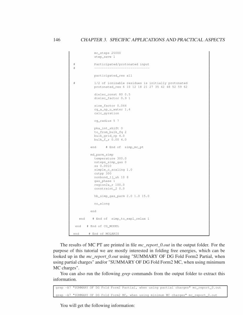
146 CHAPTER 3. SPECIFIC APPLICATIONS AND PRACTICAL ASPECTS
mc_steps 25000
step_save 1
# Participated/protonated input
# -----------------------------
participated_res all
# 1/2 of ionizable residues is initially protonated
protonated_res 6 10 12 18 21 27 35 42 48 52 59 62
dielec_const 80 0.5
dielec_factor 0.9 1
size_factor 0.044
cg_a_np_u_water 1.4
calc_gyration
cg_radius 5 7
pka_int_shift 0
to_from_bulk_fq 2
bulk_grid_rp 4.0
bulk_f_r 0.00 4.0
end # End of simp_mc_pt
md_parm_simp
temperature 300.0
nsteps_simp_gas 0
ss 0.0010
simple_c_scaling 1.0
cutpp 300
nonbond_lj_uh 10 8
gas_phase 1
region2a_r 100.0
constraint_2 0.0
hb_simp_gas_parm 2.0 1.0 15.0
no_elong
end
end # End of simp_to_expl_relax 1
end # End of CG_MODEL
end # End of MOLARIS
The results of MC PT are printed in file mc_report_0.out in the output folder. For thepurpose of this tutorial we are mostly interested in folding free energies, which can belooked up in the mc_report_0.out using "SUMMARY OF DG Fold Form2 Partial, whenusing partial charges" and/or "SUMMARY OF DG Fold Form2 MC, when using minimumMC charges".
You can also run the following grep commands from the output folder to extract thisinformation.
grep -A7 "SUMMARY OF DG Fold Form2 Partial, when using partial charges" mc_report_0.out
grep -A7 "SUMMARY OF DG Fold Form2 MC, when using minimum MC charges" mc_report_0.out
You will get the following information:

3.6. USING THE CG MODEL 147
SUMMARY OF DG Fold Form2 Partial, when using partial charges
#####################################################################################
Form2 Scaled Hydro VDW -DG POLAR Mchain DG fold
Partial size *scale UF + HB Form2
[7] [8] [9] [10] [11] [12] Partial
-------------------------------------------------------------------------------------
-8.54 12.90 -13.36 -0.41 0.11 -0.22 0.26 -9.26
SUMMARY OF DG Fold Form2 MC, when using minimum MC charges
#####################################################################################
Form2 Scaled Hydro VDW -DG POLAR Mchain DG fold
MC size *scale UF + HB Form2
[7] [8] [9] [10] [11] [12] MC
------------------------------------------------------------------------------------------
-8.54 12.90 -13.36 -0.41 0.11 -0.22 0.26 -9.26
It is the same information provided in Table 3.63 above (see entry 6 for SSO7d) . Thenumbers from the last column from the extracted output fragment (-9.26 kcal/mol in both)can be directly compared to an experimental value of -8.10 kcal/mol showing a good agree-ment. Physical meaning of different energy terms is discussed above.
A more detailed information regarding different energy terms, protonation states, in-trinsic and apparent pKa-s of ionizable residues etc. can be also found in mc_report_0.out
as was discussed in previous examples. For a detailed residue-specific summaries of elec-trostatic self-energy, polar and hydrophobic energy contributions one can also refer to filestable_ion.txt, table_pol.txt, and table_hyd.txt, respectively. MC PT run convergence can bemonitored by plotting electrostatic energy as a function of a MC step using data from thefile Energy_profile0.out. MC(Min) charges and protonation states are also reported in filecharges.out, which can be used e.g. for subsequent MC PT runs (see Example 02 below).This file contains number of particpated ionizable residues followed by lines for each ofthose residues containing residue number, name, its charge (0 or ±1), and the protonationstate (1 - protonated, 0 - not protonated).
Example 02. MC PT run for a small protein Bs_Hpr, the histidine containing proteinfrom Bacillus subtilis (PDB: 2HID) starting from a previously relaxed atomistic structure(file bs_hpr_100ps.pdb), which is read and automatically converted to the CG represen-tation with existing H atoms from the pdb removed and rebuilt (for the backbone) us-ing keepnoH keyword. 100,000 MC steps are used (mc_steps keyword). All ionizableresidues (ARG, LYS, ASP, GLU, and HIS) can participate in the MC PT (keyword partic-
ipated_res) whereas their initial protonation states are read (using file_prot_res keyword)from the file bs_hpr_charges.out, which can be generated from a previous MC PT run (typ-ially as file charges.out in the output folder, see a previous example) or created manually.This is an alternative way for specifying ionization states to using protonated_res key-word as was done in a previous example. Provided a sufficiently large number of MC stepsis used the results shold be the same or very similar but specifying most likely protona-tion states for all ionizable residues will likely result in a faster convergence. This methodshould also be used if one needs to add an effect of an electrolyte and/or external voltagea posteriori and use MC(min) charges from a previous MC PT run for these calculations.As in the previous example calculations are performed at 300 K (pt_temp keyword) and

148 CHAPTER 3. SPECIFIC APPLICATIONS AND PRACTICAL ASPECTS
at pH = 7 (ph keyword). Other keywords control simulation and force field parameters asdescribed above.
./bs_hpr_100ps.pdb keepnoH
cg_model
simp_to_expl_relax 1
simp_relax_steps 1 2
simp_mc_pt 1
ph 7
pt_temp 300.0
mc_steps 100000
step_save 1
# Participated/protonated input
# -----------------------------
participated_res all
# read a file with charges from
# a previous MC PT run
file_prot_res ./bs_hpr_charges.out
dielec_const 80 0.5
dielec_factor 0.9 1
size_factor 0.044
cg_a_np_u_water 1.4
calc_gyration
cg_radius 5 7
pka_int_shift 0
to_from_bulk_fq 2
bulk_grid_rp 4.0
bulk_f_r 0.00 4.0
end # End of simp_mc_pt
md_parm_simp
temperature 300.0
nsteps_simp_gas 0
ss 0.0010
simple_c_scaling 1.0
cutpp 300
nonbond_lj_uh 10 8
gas_phase 1
region2a_r 100.0
constraint_2 0.0
hb_simp_gas_parm 2.0 1.0 15.0
no_elong
end
end # End of simp_to_expl_relax 1
end # End of CG_MODEL
end # End of MOLARIS
The results of this MC PT run can be found in the mc_report_0.out file. As in a previous

3.7. EFFECT OF ELECTROLYTE AND MEMBRANE POTENTIAL 149
example folding free energies can be extracted e.g. by using
grep -A7 "SUMMARY OF DG Fold Form2 Partial, when using partial charges" mc_report_0.out
grep -A7 "SUMMARY OF DG Fold Form2 MC, when using minimum MC charges" mc_report_0.out
You will get the following information:
SUMMARY OF DG Fold Form2 Partial, when using partial charges
#####################################################################################
Form2 Scaled Hydro VDW -DG POLAR Mchain DG fold
Partial size *scale UF + HB Form2
[7] [8] [9] [10] [11] [12] Partial
------------------------------------------------------------------------------------
-2.77 15.89 -18.91 -0.56 -0.33 -0.81 2.70 -4.80
SUMMARY OF DG Fold Form2 MC, when using minimum MC charges
#####################################################################################
Form2 Scaled Hydro VDW -DG POLAR Mchain DG fold
MC size *scale UF + HB Form2
[7] [8] [9] [10] [11] [12] MC
------------------------------------------------------------------------------------------
-2.60 15.89 -18.91 -0.56 -0.33 -0.81 2.70 -4.63
It is the same information provided in Table 3.63 above (see entry 23 for Bs_Hpr). The numbers from the last column from the extracted output fragment (-4.80 or -4.63kcal/mol using partial or MC(Min) charges, respectively) can be directly compared to anexperimental value of -4.00 kcal/mol showing a good agreement. Physical meaning of dif-ferent energy terms is discussed above. As in a previous example file Energy_profile0.out
can be used to monitor MC PT run convergence. File charges.out contains a new set ofMC(Min) charges for ionizable residues, which are the same as the initial ones (from filebs_hpr_charges.out) in this case meaning that MC(Min) state did not change.
3.7 Effect of Electrolyte and Membrane Potential
3.7.1 Introduction
We will concentrate on Kv1.2 channel for which both open and closed conformations areavailable. Currently one needs to transform full-atom pdb to CG representation, in orderto include effect of electrolyte and membrane voltage, because model works with CG only.It is assumed by the program that channel pore and direction of the membrane potentialcoincidence withZ axis, the second important requirement is presence of the flat membranein order to calculate Videal.
If one starts from full-atom pdb protein should be rotated so pore is in Z direction, thenfull-atom protein should be converted to CG representation, and finally membrane shouldbe built and membrane atoms inside pore and cavities should be deleted and after that oneneeds to check that the membrane is flat.
Equilibration regimes for calculation of thermodynamic stability and gating charge aredifferent. Two sides of electrolyte are ether equilibrated together or separately.

150 CHAPTER 3. SPECIFIC APPLICATIONS AND PRACTICAL ASPECTS
All the files required for the run and additional files with model description can befound in molaris demo directory in subdirectory voltage/barrier. It has not only voltagefiles but also necessary steps for creation of the intermediate. At present moment it takesup to an hour for complete run of the simulation, but one can update submit.pbs script inorder to run only one structure for a given membrane potential. File sampleResults hassample output from the simulation after running of the totalEnergy.sh script. It should benoted that with future molaris model and with development of the CG model, energeticsmay change, but change in stability of structures should be checked.
3.7.2 Input Files Description
The main part of the input file is similar to the regular CG input file with additional de-scription of the electrolyte and membrane voltage as well as coupling to CG free energy.At present simulation protocol consist of two runs: first CG simulation coupled to mem-brane potential is performed till minimum of free energy is achieved, during the second runcoupling between CG and electrolyte is switched on. For the first run approximately 10000to 50000 steps is usually enough to achieve convergence (in case of Kv1.2). At presentelectrolyte subroutine is called each MC step and it is computationally intensive, that iswhy electrolyte-coupled simulations (second run) is performed for only 10 MC steps.
OPENED_membrane.pdb
analyze
#charge_zwit_membrane Z 0.1 -0.1
ionic_grid
voltage -0.2
ig_rec_for_membrane 80. 80. 400. 5. 10.0 0.15 0.15 80.0
period 0
run_mc_pt 1
equilibration 1
numberOfIterations 0
step0 0.01
K_equilibration 10.0
#write_restart 200.rest
#read_restart 1000.rest
end
simp_to_expl_relax 1
# ... part deleted for brevity
# as in regular MC for CG model
exclude_e_bat
simp_mc_pt 1
ph 7.0
mc_steps 1000
step_save 1
participated_res 2 3 12 14 18 25 30 32 33 34
# ... see demo file for all participated resiues (deleted for brevity)
participated_res 1518 1527 1558 1559
file_prot_res charges.out
# ... part deleted for brevity
# as in regular MC for CG model
end # End of simp_mc_pt
md_parm_simp
# ... part delted for brevity
# as in regular MC for CG model
end
end # End of simp_to_expl_relax 1
end # End of Analyze
end # End of MOLARIS
3.7. EFFECT OF ELECTROLYTE AND MEMBRANE POTENTIAL 151
One can see that input file is exactly the same as for regular CG when one run CGon analyze level (as first implemented in Molaris) with the exception of addition of thelevel ionic_grid. This new level describes electrolyte interaction with protein charges andmembrane potential.
Here we describe all the keyword on the ionic_grid level. Keyword voltage describesdifference in the membrane potential for two electrolyte solutions in volt, it is assumed thatpotential is a difference between potential from electrolyte solution on the left (smaller Zcoordinates) and potential of the right (larger Z coordinates) solution. For the developer,it should be noted that most of the actual calculations are done in kcal, so care should betaken in units conversions while reading source code.
The main keyword is ig_rec_for_membrane specifies box size of electrolyte, this gridis build around center of the system, next vdw cutoff for grid and protein or membraneatom is specified followed by spacing for the grid. And then concentration of electrolyte inthe left and right compartments is defined and the last number is dielectric constant.
The keyword period defines number of periodic images of grid in x, y directions. It hasbeen tested on electrolyte solution and electrolyte with membrane but not with protein inthe system.
The keyword run_mc_pt 1 specifies that electrolyte-voltage coupling is done with MCPT, run_mc_pt 0 allows one to run subroutine on analyze level without MC PT but onlywith uncharged ionazable residues (can be used for debug purposes).
The keyword equilibration 1 forces two sides of electrolyte to equilibrate, equilibration
0 forces separate equilibration of two electrolyte compartments.The keyword numberOfIterations defines number of iteration for electrolyte equilibra-
tion.The keyword step0 specifies generation of the next electrolyte charges from the current
charges.The keyword K_equilibration defines additional potential used for faster convergence.Additional keywords write_restart and read_restart add ability to save electrolyte
charges in restart file.All other keywords are standard. After run is done with above mentioned input file we
need to switch electrolyte coupling, for this purposes we run additional simulation withinput file where numberOfIterations 100 to allow equilibration of electrolyte and mc_steps
10, everything else stays the same. If during the first run one specifies file_prot_res differentfrom standard name charges.out one also need to change it.
3.7.3 Output files
After MC PT is performed, followed by several steps of MC PT coupled to electrolyte-voltage subroutine final free energy of the system can be found in mc_report_0.out.
This output file is standard MC PT run with additional information about electrolyteenergy and effect of electrolyte and membrane voltage on pKi. Two additional lines added.First electrolyte energy is printed, followed by sum of MC PT free energy and electrolyteenergy.

152 CHAPTER 3. SPECIFIC APPLICATIONS AND PRACTICAL ASPECTS
...
[1]+VQQ_partial+[7]+[8]+[9]-[10] 36.52
FORM2 +[8]+[11]-[10](TOTAL) -176.97
Electrolyte term 10.03207690887927
TOTAL ENERGY(MC_PT+electrolyte) = -166.9405453367622
[12] Average VQQ (hopefully it is correct) NaN
-------------------------------
-------------------------------
SUMS of Minimum MC charges
...
3.8 Langevin Dynamics Simulation of Ion Channels
3.8.1 Introduction
Program Channelix was written by group members of Prof. Warshel lab for studies of ionchannels, but it is also possible to use this program as a general Langevin Dynamics (LD)program for the systems without chemical bonds (which cause problems in integrationalgorithm at present).
It is assumed that the pore is in z direction and that the center of the pore has x = 0, y =0 coordinates. Coordinate system is the consistent for all input files.
Program can be run from command line as usual and all input and output files will bein the current directory:
./channelix<gramicidin.inp>gramicidin.out
3.8.2 Input Files Description
Let’s explain setup of input files for the system schematically shown on the figure 3.15. Itrepresents gramicidin A channel in the membrane but the free energy barrier through thepore is artificially lowered to allow fast simulation.
The main input file is gramicidin.inp contains main information and also specifies in-formation about all other input files. The name of the file is actually not important andcan be changed. The sequence of commands is important as well as four initial commentslines, order should be keep the same otherwise information will not be parsed correctly.
First 4 lines of gramicidin.inp are required comments, next line is dt for integrationalgorithm, then mass of the ion (at present only one ion type is allowed and mass is thesame for cation and anion), then friction coefficient, temperature, total number of LD stepsand frequency for writing data to files.

3.8. LANGEVIN DYNAMICS SIMULATION OF ION CHANNELS 153
Figure 3.15: Gramicidin and system geometry

154 CHAPTER 3. SPECIFIC APPLICATIONS AND PRACTICAL ASPECTS
########################################################################
# CHANNELIX 2.0 #
########################################################################
# #
0.001 #dt psec
23.0 #m amu
8 #g psec(-1)
300.0 #temp K
1000000 #n steps
10000 #j save steps
FreeEnergy.dat # free energy profile (DELETE comment for run)
SodiumClorides.dat # ions in the system (DELETE comment for run)
ionazableRes.dat # fixed chagred residues (DELETE comment for run)
gramicidin.dat # information about channel geometry (DELETE comment for run)
./ # output directory (DELETE comment for run)
F # wall
F # cylinder and membrane
T # charges
F # solv
T # ion pulling
T # lang_type ! change for regime
0.0 #potenital in mV
0.0 #potential in mV
0.2 50 # K pulling z0 for pulling
# T= kill interactions (wall,cylinder,charges,vdw,solv,mb)
#
#lang_type=T dt*g<<1 under
# =F dt*g>>1 over
#
The file gramicidin.inp defines files with free energy profile FreeEnergy.dat, ions thatare movable SodiumClorides.dat, fixed ionazible residues of the protein ionazableRes.dat
(not used or tested), and information about system and channel geometry gramicidin.dat.Please note that for the actual run one need to delete comments (starting with #) for linesspecified in the input (this is technical limitation due current parsing approach).
Then there are logical variables that specify presence or absence of specific interac-tion, here order again is of importance. wall means interaction of the ion(s) which keepit within the cubic system, cylinderandmembrane describes repulsive interaction of themembrane and pore of the channel (in x,y directions), chagres switches off/on explicitcharge-charge interactions with ions from ionazableRes.dat, solv describes solvation pro-file in pore(z-direction), ionpulling switches on/off additional pulling potential. For all ofabove mentioned logical variables F means keep interaction, T means switch interactionsoff.
Last logical variable describes underdump or overdump integration mechanism, as canbe seen from the comment.
Next two lines describes external potential in the left compartment(z < zcenter) and onthe right(z > zcenter), linear potential approximation is use for the pore/ membrane region.This is used for simulation of the membrane potential.
Pulling potential is described by:
Upull = K · (z − z0)2
and used as a way to accelerate dynamics of the system as in SMD approach.File FreeEnergy.dat contains free energy (in kcal) profile for z coordinate of the pore
and also specify number of points in the profile (linear interpolation is used for the inter-

3.8. LANGEVIN DYNAMICS SIMULATION OF ION CHANNELS 155
mediate z values). Profile is also plotted on figure 3.16, it is artificially too low to get fastertransition through the pore.
0
0.1
0.2
0.3
0.4
0.5
0.6
0.7
0.8
0.9
1
-15 -10 -5 0 5 10 15
Fre
e E
nerg
y (k
cal)
z (Angstrom)
exp(-0.03*x**2)
Figure 3.16: Free Energy profile in z direction
#31
-15.000000 0.001171
-14.000000 0.002795
...
-3.000000 0.763379
-2.000000 0.886920
-1.000000 0.970446
0.000000 1.000000
1.000000 0.970446
2.000000 0.886920
3.000000 0.763379
...
14.000000 0.002795
15.000000 0.001171
File SodiumClorides.dat contains coordinates of positive and negative ions which canmove (diffuse) in the system. The first line specifies total number of ions in the system,second line specifies how many ions can move through the channel, for the rest there isrepulsion from the pore entrance. It should be noted that although name of the ion isrequired it is not used and only important data are charges and coordinates. Also at presentmass is from gramicidin.inp file. In the current simulation only Sodium ions can movethrough the pore.
#4
#2
K 1.000 0.000 0.000 -16.000
K 1.000 0.000 0.000 50.000
Cl -1.000 0.000 0.000 -50.000
Cl -1.000 0.000 0.000 20.000
It is possible to specify additional fixed charges for the system in file ionazableRes.dat,although it is computationally expensive. This file is not used for gramicidin and put herejust as example of the format.

156 CHAPTER 3. SPECIFIC APPLICATIONS AND PRACTICAL ASPECTS
#5
-1.00 15.909 8.000 13.682 29 GLU
1.00 24.370 1.768 16.866 30 ARG
1.00 18.861 -2.335 18.814 42 ARG
-1.00 8.167 -3.061 13.573 58 ASP
1.00 2.383 -23.520 17.965 127 ARG
File gramicidin.dat contains information about the geometry of the channel and thesystem. The first two lines are required comments, then x,y,z ranges are defined as infigure 3.15. Next we specify boundary for the pore of the channel and dimensions of themembrane(but membrane dimensions are not used at present).
For channels like KcsA, Kv1.2 geometry of the pore is more complicated than simplecylindrical pore of the gramicidin, e.g. in Kv.1.2 there are three distinct regions: selectivityfilter, cavity and gate. These regions has different pore radii. That’s why next line specifyhow many such regions do we have - one for the case of gramicidin. And the followinglines (again one for gramicidin) define such a regions. First number is the end of thecurrent regions, the start is implicitly calculated as either start of the pore(MINCHANZ) orprevious region. And the last two numbers are pore radius for the given region and forceconstant for repulsion from the walls of the pore.
# file contains infromation about ion channel
# geometry and geometry of the system (channelix2.1 ver)
-50 50 #XMIN and XMAX
-50 50 #YMIN and YMAX
-100 100 #ZMIN and ZMAX
-15 15 # MINCHANZ and MAXCHANZ
-15 15 # MBZMAX and MBZMIN (assume that x,y dimens. correspond to XMIN,...)
1 #number of parts of the channel with different radius
15 4 5
All files described above are required for the simulation even if some features are notused.
3.8.3 Output files
After all input files correctly parsed channelix performs LD for all ions specified in theSodiumClorides.dat. Let’s here describe several important output files and the data in them.For the sake of brevity blank line is the output files were deleted to save space.
File gramicidin.out (or in geenral results from stdout) contains general ionfomraionabout timing of the run and also information about succesesful movement of the ion(s)through the pore.

3.8. LANGEVIN DYNAMICS SIMULATION OF ION CHANNELS 157
Program CHANNELIX: Oct 25 2010
===================================================
Reading input files: Time: Mon Apr 30 16:14:49 2012
===================================================
Killing CHARGE
Killing ion pulling
..dt*g<<1 regime...
Intracellular Potential (mV) 0.000000000000000
Extracellular Potential (mV) 0.000000000000000
FreeEnergy.dat
SodiumClorides.dat
ionazableRes.dat
gramicidin.dat
ions coordinates have been read ...
File with channel geometry has been read
solvation potential coordinates have been read ...
===================================================
Reading is finished: Time: Mon Apr 30 16:14:49 2012
===================================================
sigma = 30477.72575100492
sigma2 = 1.6359487789052562E-002
===================================================
Calculations begin: Time: Mon Apr 30 16:14:49 2012
===================================================
===================================================
Calculations are finished: Time: Mon Apr 30 16:15:06 2012
===================================================
File with name current.dat has information about convergence of current as functionof time. First column is time and second column is ion current. Significantly longer runrequired to get passage of the ions through the pore and till Ohm’s law will be satisfied.
0.00000 NaN
6.47800 0.0
6.47800 0.0
...
979.99900 0.0
989.99900 0.0
999.99900 0.0
File number.dat provides data about ions position in the system. Ions are either in theleft compartment, pore or right compartment.
0.00000 1 1 0
9.99900 0 1 1
19.99900 0 1 1
29.99900 1 1 0
39.99900 1 1 0
49.99900 1 1 0
59.99900 1 1 0
69.99900 1 1 0
...
File pass.dat has data for ion passage for each compartment.
0.00000 0 0
6.47800 0 0
6.47800 0 0
9.99900 0 0
...
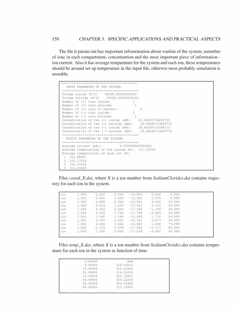
158 CHAPTER 3. SPECIFIC APPLICATIONS AND PRACTICAL ASPECTS
The file it param.out has important infomrmation about voulme of the system, numnberof ionc in each compartment, concentartion and the most important piece of information -ion current. Also it has average temparature for the system and each ion, these temperaturesshould be around set up temperature in the input file, otherwis most probably simulation isunstable.
*****************************************INPUT PARAMETRS OF THE SYSTEM:
*****************************************Volume inside (A^3) 56000.00000000000
Volume outside (A^3) 56000.00000000000
Number of (+) ions inside: 1
Number of (+) ions outside: 1
Number of (+) ions in channel: 0
Number of (-) ions inside: 1
Number of (-) ions outside: 1
Concentration of the (+) inside (mM): 29.64285714285715
Concentration of the (+) outside (mM): 29.64285714285715
Concentration of the (-) inside (mM): 29.64285714285715
Concentration of the (-) outside (mM): 29.64285714285715
*****************************************OUTPUT PARAMETRS OF THE SYSTEM:
*****************************************Average current (pA): 0.000000000000000
Average temperatures of the system (K): 311.62318
Average temperatures of each ion (K):
1 312.68987
2 310.13329
3 312.37666
4 311.29289
Files coord_X.dat, where X is a ion number from SodiumClorides.dat contains trajec-tory for each ion in the system.
ion 1.000 0.000 0.000 -16.000 0.000 0.000
ion 1.000 0.630 3.650 -13.962 0.078 9.999
ion 1.000 2.690 2.962 -14.841 4.046 19.999
ion 1.000 3.919 1.530 -17.831 -3.141 29.999
ion 1.000 4.269 2.092 -17.186 -1.199 39.999
ion 1.000 6.515 1.740 -17.780 -4.983 49.999
ion 1.000 7.598 1.240 -15.649 1.716 59.999
ion 1.000 3.797 2.991 -15.541 3.673 69.999
ion 1.000 0.090 1.446 -16.820 1.848 79.999
ion 1.000 -1.733 0.039 -17.202 -2.717 89.999
ion 1.000 1.035 0.040 -17.238 -4.602 99.999
Files temp_X.dat, where X is a ion number from SodiumClorides.dat contains temper-ature for each ion in the system as function of time.
0.00000 NaN
9.99900 328.00014
19.99900 315.51859
29.99900 314.59204
39.99900 310.33967
49.99900 309.22200
59.99900 309.59408
69.99900 313.10663
...
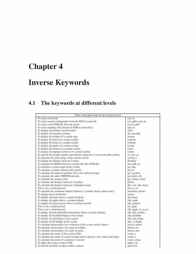
Chapter 4
Inverse Keywords
4.1 The keywords at different levels
Table of the Keywords for the Analyze LevelTo read a restart file rest_inTo read a certain configuration from the PDLD restart file rest_pdld_conf_inTo create a new PDB file from the restart rest_to_pdbTo read a topology file (instead of PDB or restart files) topf_inTo display all residues current loaded allresTo display all ionizable residues all_ionizableTo display all residues of a certain type restypeTo display all atom sof a certain residue resatomTo display all bonds of a certain residue resbondTo display all angles of a certain residue resangTo display all torsions of a certain residue restorTo display all improper torsions of a certain residue resitorTo specify the residue number and effective dielectric of a non-ionizable residue res_ion_vqTo calculate the total energy of the current system system_eTo display the distance between 2 atoms distatomTo calculate the RMSD between a restart file and a PDB file rms_pdb_resTo calculate a certain angle in the system get_angTo calculate a certain torsion in the system get_torTo calculate the radius of gyration (for a user defined group) get_gyrationTo calculate the native HBOND network get_native_hbTo calculate the contact order get_contact_orderTo calculate the distance between 2 residues distresTo calculate the distance between 2 sidechain atoms dist_cen_side_heavyThis is not a valid keyword dist_ca_caTo calculate the minimum distance between 2 residues (heavy atoms only!) minimum_distresTo change atom coordinates setxyzTo diaplay all bonds above a certain treshold chk_bondTo display all angles above a certain treshold chk_angleTo display all main torsions above a certain treshold chk_maintorThis is not a valid keyword set_angleThis is not a valid keyword chk_angle_ca_ca_caTo display all bad nonbonded interactions below a certain distance chk_bad_nonbd_rTo display all disulfide bridges in the system chk_disulfideTo display all salt bridges in the system chk_salt_bridgeTo display all SS bridges in the system chk_ss_bridgeTo calculate electrostatics for a selection of the system inside radius r electro_radiusTo calculate electrostatics for a pair of residues electro_resTo calculate electrostatics for a pair of atoms electro_atmTo calculate the center of the system (CM) center_sTo calculate the center of a given residue and to specify a new center and radius center_rTo calculate the center of a selection of atoms center_atomsTo adjust the center of mass (CM) adjust_cmTo find all ionizable residues within a sphere sphereion
159

160 CHAPTER 4. INVERSE KEYWORDS
To find all residues within a radius from a center sphereresTo find all atoms within a radius of a center sphereatmTo add a new bond between two atoms addbondTo display all bonds for an atom bonds_for_atomTo display all angles for an atom angles_for_atomTo remove a bond between atoms removebondTo render an atom dummy set_atom_dummyTo move a group of atoms move_atomsTo mutate a residue mutate_resTo mutate to a simplified residue (from simplified or explicit representation) mutate_simp_resTo mutate a residue to H2O mutate_res_to_h2oTo rotate hydrogen bound to heavy atoms rotate_hTo rotate an atom rotate_atomTo rotate the axis rotate_axisTo rotate a helix rotate_helixTo make coordinate files from the movie binary file viewmovieTo create files for viewing the electrostatic potential surface for region 1 viewpotTo calculate the VDW surface area of the protein vdwsurfTo create a new PDB file from the current system makepdbTo make a new toplogy file of the current system maketopTo make a new PDB file from 2 PDB files (by mixing_lambda) makepdb_from_2_pdbTo make a new PDB file from a restart file makepdb_from_restTo make a new PDB file from QM output makepdb_from_qmTo make a new library entry makelib1To translate the whole system translate_systemTo replace a solute molecule in the system replace_ligandTo rigidly align CA of the current system with the CA of a PDB file superimpose_ca_pdbTo rigidly align CA of the current system with the CA of restart file superimpose_ca_restTo list all HBONDS in a defined cutoff cutoff range for that bonds list_hbondsTo list all HBONDS that exist in the current structure and a restart file list_hbonds_2To return the residue number an atom belongs to whichresTo compare the residues numbers between current system and PDB file pdb_res_to_mol_resTo uncharge the residues chraged from the amber library uncharge_amberTo convert the CG model to the alfa-beta model cg_to_alfa_betaTo calculate the non-bonded pairlist for specified CG residues cb_nonbond_listTo add main chain atoms add_main_atomsTo add sidechain atoms add_sidechainTo minimize added sidechains using the steepest descent method minimize_sideTo convert simplified residues to explicit structures simp_to_expl_pdbTo convert and relax simplified residues to explicit structures simp_to_expl_relaxTo relax with 2 PDB structures – Ask Dr. Chu here expl_pdb_2_relaxTo ionize all resiues of the specified type iontypTo ionize simplified residues of a specified type ion_simp_typeTo ionize united residues of a specified type ion_united_typeTo add electrodes to the system add_electrodesTo add a membrane grid to the system add_memgridTo add membrane electrodes to the system add_mem_electrodesTo dock a ligand into a binding site dock_ligandTo define region1 atoms reg1_atmTo add a layer of membrane grid around the surface of specified region 1 atoms add_memgrid_surfaceTo remove membrane atoms within a sphere or cylindrical space remove_mem_rTo remove membrane atoms within a cubic or recangular space remove_mem_xyzTo charge membrane atoms (top and bottom layers along a specified axis) charge_membraneTo build a LD grid around the system ld_for_membraneTo build an ionic grid around the system ig_for_membraneTo add a new C-terminal residue add_res_at_endTo add a new N-terminal residue add_res_at_startTo insert a new residue at a specified position insert_resTo remove a residue at a specified position remove_resTo print the group correlation matrix write_grp_corrTo calculate the autocorrelation auto_correlationTo update the topology file update_topologyTo generate a histogram from an external file general_histogramWe need more explanation here, too big calculate_w_ele_vdw
Table of the Keywords PRE_ENZ LevelTo ionize a certain residue ionresTo half-ionize a certain residue ionres_halfTo half-ionize all residues of a certain type iontyp_half

4.1. THE KEYWORDS AT DIFFERENT LEVELS 161
To unionize a certain residue unionresTo ionize all residues of a certain type iontypTo ionize all DNA residues inside a given radius with -1 ion_phosphateTo ionize all residues of a certain simplified type ion_simp_typeTo set a new charge for a specified atom setcrgTo set the charge to zero for specified residues setcrg0To set teh charge to zero for every mainchain atom in a specified residue set_maincrg0To change atom coordinates setxyzTo charge membrane atoms (top and bottom layers along a specified axis) charge_membraneTo calculate electrostatics of a region1 residue with region2 electroTo read a restart file rest_inTo use atomic coordinates from a restart for constraints rest_constrTo create a new PDB file from the current system makepdbTo display all atom sof a certain residue resatomTo display all bonds of a certain residue resbond
Table of the Keywords RELAX LevelTo change default MD parameters md_parmTo read a restart file rest_inTo create a restart file rest_outTo change the default frequency for energy printout (default is every 10 steps) energy_outAsk Dr. Chu what this here does relax_map_lambdaTo define all residues in region 2 region2_resTo specify the steps to map the free energy profile map_pfI have no clue what this means mutate_to_GLYTo specify the relax mapping for unfolding (from folded) relax_map_unfoldTo calculate the protein energy of explicit and simple residues explicit_simpleThis is not a keyword! cal_dely2_uuTo enter the level for specifying the parameters used in the simple form expl_simp_parmTo print the energy and RMSD in the gap files for a relaxation run write_gap_rmsTo minimize added sidechains using the steepest descent method minimize_sideTo minimize the main torsion in the protein minimize_main_torTo specify the minimum system energy for minimizing sidechains minimize_run_parmTo specify the gyration constraint on CA for state 1 relax_map_gycon1To specify the gyration constraint on CA for state 2 relax_map_gycon2To specify the center corrdinates for gyration calculations gyration_centerTo relax 2 states of different harmonic distance constraints for 2 atoms relax_map_consTo relax from an unconstrained torsion to constrained torsion relax_map_torTo specify initial and final postions of the atom for the relax mapping relax_map_pmf_zTo relax with protein native-contact order constraint for simple system relax_map_contactTo relax with native HBOND constraints relax_map_native_hbTo define the plus factor for the native contact order contact_native_rTo calculate the protein contact order for explicit structures explicit_contactTo specify the scaling factor in contact order calculations multi_contact_vdwTo specify the scaling factor for vdw energy in relaxation runs multi_relax_vdwTo calculate electrostatics between substrate and the remainder of the system substrate_resTo specify the dielectric constant for substrate and sidechain atoms diele_sub_sideTo alter electrostatic and self-energy print frequency of ionized residues simp_grp_contrib
Table of the Keywords AC LevelTo define region 1 residues reg1_resTo define region 1 atoms reg1_atmTo assign the charges for states 1 and 2 ab_crgTo assign VDW parameters for states 1 and 2 ab_vdwTo modify VDW parameters using softcore potentials soft_dummy_vdwTo change default MD parameters md_parmTo supply charges and VDW parameters in a file read_acTo set the mapping parameter from state A to B map_lambdaTo set the number of frames for the free energy profile map_pfTo set the entropy constraint for AC calculations ac_entropyTo print the step interval for energy printout write_w_ac_fqTo read in a restart file rest_inTo write a restart file rest_outTo set the frequency of writing restart files rest_fqTo use coordinates from a restart file for constraints rest_constrTo specify positionsal constraints in AC calculations atom_p_conTo print the energy output energy_outTo write out the force on AC atoms check_fTo morph AC atoms during an AC calculation atom_B_shrinkTo set the frequency to print non-bonded interactions write_nonb_fq

162 CHAPTER 4. INVERSE KEYWORDS
To set the frequeny to print non-bonded interactions between 2 AC atoms/groups write_nonb_grpTable of the Keywords EVB Level
To request an EVB run evb_simpTo define EVB parameters evb_parmTo monitor electrostatics between an EVB(s) atom and the system evb_grp_elecTo calculate electrostatics between an EVB an dprotein group evb_pro_grp_elecTo set the number and density of resonance states evb_stateThis is not a valid keyword!!! mutating_evb_atomsTo set the evb atoms to be mutated to aqueous oxygen evb_mutated_to_woTo add an atom to the EVB region evb_atmTo request TS mutation (to dummy) evb_ts_mutateTo request TS charging calculations evb_ts_chargingTo set the densities of the TS evb_ts_densityThink about this general_ts_mut_mapTo be used with other keyword evb_ts_II_0_atmTo specify evb state without electrostics with environment no_elec_stateTo assign EVB torsional force constants pi_tor_pijTo assign a dummy and screen parameter dummy_evb_screenTo assign the bond length of the dummy (to be shrinked) d_evb_bond_shrinkTo set charges for linked protein atoms for different EVB states link_p_crgTo switch to harmonic bond calculation (instead of Morese potential) bond_harmonicTo use an extra harmonic bond force harmonic_morseTo assign an EVB bond between 2 atoms evb_bndTo assign a distance range constraint for EVB atoms evb_d_range_conTo assign a distance constraint between 2 EVB atoms evb_d_conTo assign an angle constraint for EVB atoms evb_a_conTo assign a torsional constraint for EVB atoms evb_t_conTo get the added constraint for adiabatic evb energy profiles ave_2pdb_conTo assign a positional constraint for EVB atoms evb_position_conTo assign a distance constraint for EVB and protein atoms evb_protein_conTo force the atom movement along a vector vector_a_conTo assign PENTACOORDINATES pentacoordTo assign the D parameter for pentacoordinated atoms penta_ang_DTo switch to an uphill to TS calculation uphill_to_tsTo perform an LRA run for EVB at the TS lra_evb_tsTo calculate the LRA VDW contribution from each protein residue lra_grp_vdwTo assign the part of the system for entropy calculations evb_entropyTo calculate average electrostatics of each residue to each resonance state ave_elecTo calculate electrostatic contribution of main and sidechain atoms chain_ele_stateTo set the number of steps to construct the free energy profile map_pfTo assign the gas phase dG for the given EVB state gas_dgTo assign the 2 atom off-diagonal element HijTo assign the 2 atom off-diagonal element Hij_2To specify the off-diagonal parameter for calculating Hij Hij_gapTo specify the off-diagonal parameter for calculating Hij Hij_gap_cTo specify the 3 atom off-diagonal elements HrTo specify 3 atom off-diagonal elements Hr_gaussTo switch to different mapping potential ADV_EVB_MAPTo recalculate the Borgis off-diagonal elements H3To recalculate the Borgis off-diagonal elements H3_2To assign inductive interactions R4To select inductive mode intra_evb_induceTo specify certain exponential coefficient exponentialTo calculate VDW between evb and protein atoms vdw_evb_pTo define type of VDW parameters for evb and protein atoms vdw_evb_p_typeTo calculate nonbonded interaction between a pair of atoms vdw_pairTo delete an angle between EVB atoms kill_angTo add a new angle between EVB atoms (or atoms) add_angTo set a new angle between EVB atoms (or atoms) set_angTo delete a specific torsional contribution kill_torTo add a new torsional parameter for EVB atoms (or atoms) add_torTo add a new improper torsional parameter for EVB atoms (or atoms) add_itorTo add a new torsional parameter using a harmonic function harmonic_torTo add new morse bond parameters morse_pairTo read an existing EVB file read_evbTo read in a restart file rest_inTo create a restart file rest_outTo set the frequency a restart file is written rest_fq

4.1. THE KEYWORDS AT DIFFERENT LEVELS 163
To write restart files at specified intervals rest_stepTo create a series of restart files for a defined EVB state ad_restoutTo use coordinates from a restart filr for consraints rest_constrTo switch on automatic proton transport calculation proton_transportTo define H3O charges for the proton transport pt_h3o_chargesTo define H2O charges for the proton transport pt_h2o_chargesTo define H3O EVB types for proton transport pt_h3o_evbtypeTo define H2O EVB types for the proton transport pt_h2o_evbtypeTo define the 3 off-diagonal for O..H-O (Borgis) pt_off_h3To switch on rigid bond energy mapping of reactions in gas bond_rigid_mapTo switch on rigid bond energy mapping of reaction in water rigid_map_in_waterTo define starting and ending atoms of a rigid bond mapping move_rigid_mapTo invoke the centroid level centroidTo define the target temperature in the xentroid run centroid_tempTo invoka a centroid DISPOLARON calculation centroid_dpThis is not a valid keyword centroid_write_xTo define the EVB atoms to add the Gaussian Bias energy centroid_gaussianTo define DP dipole solvents dp_file_nameTo define coupling of cross terms in EVB use_ba_couplingTo request paradynamic refinement of EVB parameter refine_use_dfdp1To refine an EVB bond refine_evb_bondTo refine an EVB angle refine_evb_angleTo refine an EVB torsion refine_evb_torsionTo refine an EVB imporper torsion refine_evb_itorsionTo refine an EVB VDW parameter a refine_evb_vdw_aTo refine an EVB VDW parameter b refine_evb_vdw_bTo refine the EVB hij parameter a for a specified hij refine_evb_hij_aTo refine the EVB hij parameter mu for a specified hij refine_evb_hij_muTo refine the EVB hij parameter mu for a specified hij refine_evb_hij_muTo refine the EVB hij parameter a for a specified hr refine_evb_hr_aTo refine the EVB hij parameter mu for a specified hr refine_evb_hr_muTo refine the EVB hij parameter a for a specified h3 refine_evb_H3_ATo refine the EVB hij parameter alpah for a specified h3 refine_evb_H3_ALFATo refine the EVB hij parameter beta for a specified h3 refine_evb_H3_BETATo refine the EVB hij parameter gamma for a specified h3 refine_evb_H3_GAMATo define gas phase shift for refinement refine_evb_gas_shiftTo define nonbonded exponential repulsion parameter expl_repl for refinement refine_evb_nb_expTo define nonbonded exponential replusion parameter beta for refinement refine_evb_nb_betaThis is not a valid keyword refine_evb_nb_a_pairTo specify the EVB electro screen parameter for refinement refine_evb_screenTo specify the number of PDB files and the root file pdb_file_for_refineTo specify the restart file (QM) to be used in evb parameter refinement rest_file_for_refineTo specify QM force file root name Fq_file_for_refineTo specify files in xyz format for PD refinement xyz_file_for_refTo specify the force_file for PD refinement force_file_for_refTo specify quantum energies for PD refinement Eq_file_for_refineTp specify the values for k1 and k2 in the minimiziation k1_k2_for_refineTo specify the number of steps and stepsize in SD minimization for refinement ref_steepest_stepsTo specify the dp scaling factor in the Paradynamics refinement of EVB use_ref_dpTo write out the probability of each evb state write_probTo writes out numerical and analytical force on evb atoms check_fSpecialized EVB section for proton transfer evb_sectionTo be used with evb_section transition_sectionTo switch off calculation of electrostatics for EVB atoms no_elec_forceThis is not a valid keyword write_res_crgTo specify the vq of each evb atom with protein and water atoms write_vq_out
Table of the Keywords MD_PARM LevelTo set the number of steps NSTEPSTo set the temperature TEMPERATURETo define the tolerance temperature TOLERANCE_TEMPTo define multiple steps in temperature MULTI_TEMPSTo define the stepsize [ps] STEPSIZETo define multiple stepsizes MULTI_STEPSIZETo change the stepsize during the run CH_STEPSIZETo specify the number of extra relaxation steps RELAX_1To specify that no automatic relaxation no_auto_relaxThis is not a valid keyword auto_relax_stepsTo set the frequency of updates of nonbonded interactions nbupdate

164 CHAPTER 4. INVERSE KEYWORDS
To run in the gas phase GAS_PHASETo remove bulk water NO_BULKTo define the radius for region2 REGION2A_RTo define the radius for the water solvent grid WATER_RTo define the distance of water to membrane atoms WATER_MEM_RTo ionize all ionizable residues in region 2 ion_reg2 0.5To define the langevin grid LANGEVIN_RTo specify the radius for thermalizable atoms thermalize_rTo specify the exclusion and water grid center coordinates ex_w_centerTo print all reswidues in a specified layer write_res_in_surfTo print waters around certain residues write_wat_from_resTo set the solvent solventTo switch on inductive forces induceTo specify the screen parameter in the induced dipole calculdation induce_screenTo set the dielectric constrant to screen electrostatic interaction electro_screenTo switch the calculation of the induced force on or off indforceTo switch on induction for ac atoms induce_ac_atomsTo calculate VDW interactions using defined parameters A & B p_pair_vdwTo calculate VDW interactions using defined parameters e and r p_pair_vdw_erTo switch off electrostatics between certain residues no_electro_pairTo specifying a start and end configuration for constraining pdb constraint_1_pdbTo define constraints for region 2 atoms CONSTRAINT_2To define constraints for water molecules CONSTRAINT_WTo define distance constraints for 2 sets of atoms CONSTRAINT_2DTo constraint the distance between a pair of atoms CONSTRAINT_PAIRTo define position constraints for an atom CONSTRAINT_POSTTo define a position constraints for atom and a point CONSTRAINT_RTo define an angular constraint CONSTRAINT_ANGTo define a torsional constraint CONSTRAINT_TORTo define a positional constraint on mainchain atoms CONSTRAINT_MAINTo define constraints for main torsions CONSTRAINT_MAINTORTo define positional constraints for a residue CONSTRAINT_RESTo define positional constraints for an atom CONSTRAINT_ATMTo define constraints for helix torsions and hbonds HELIX_CONSTRAINTTo constraint H atoms in their original positions H_CONSTRAINTTo use the SHAKE method for 2 atoms SHAKE_CONS_DISTTo define the SHAKE parameters SHAKE_PARAMETERTo use atomic coordinates from a restart for constraints rest_constrTo specify the distance and constraint force for region 1 atoms region1_plus_consTo specify the frequency of printing xyz coordinates write_atom_xyzTo set the frequency a restart is being written REST_FQTo set the frequency a restart file is being updated rest_update_fqTo record a binary to allow for movie creation MOVIE_COTo set the movie frequency written to the binary file MOVIE_FQTo request a quasiharmonic estimate of the entropy QUASIH_ENTROPYTo specify the 2 states for the RR approach RR_STATETo specify the force constants for the RR approach RR_FORCETo specify the force constant for the quasiharmonic approach RR_QUASIHTo specify the restart files for a RR calculation rr_restartTo set several parameters for RR calculations rr_prepTo specify LD with 2 solvents and user-defined reorganization energy langevin_chem_confTo specify Hij for running langevin_chem_conf lan_chem_conf_HijTo specify the gas-phase shift for running langevin_chem_conf lan_chem_conf_gasThis is not a valid keyword lan_chem_conf_fqTo request a LD simulation langevin_dynTo assign dummy properties to an atom dummy_atomTo specify the gamma parameter in LD simulations lan_dyn_gammaTo specify solevnt dipoles in LD simulations sol_evb_dipoleTo specify initial coordinates for each solevnt in sol_evb_dipole x_sol_0To specify the coupling of langevin dipole solvents sol_evb_coupleTo start a user-defined child run from a parent EVB run evb_calloutTo gather energies (for paradynamic runs) evb_wrefTo specify mass, force constant and gamma for added conformation langevin dipole conformation_mkxgTo specify constants in conformation energy calculations conform_u_parmsTo define the langevin solvent coupling strength qq_couple_factorTo specify the file for langevin solvent coordinates sol_file_nameTo request the use of implicit solvation exp_implicit_svTo specify the input file for doing helicase calculations helicase_file

4.1. THE KEYWORDS AT DIFFERENT LEVELS 165
This is not a valid keyword fdftTo invoke the QMMM level (region 1 atoms are treated by QM) qmmmThis is not a valid keyword qcffEvaluate the PMF by moving from initial to final state pmfTo specify the radius of gyration constraint of CA atoms gyration_consTo specify the PMF mapping ub_samplingTo freeze all atoms of a certain region FIX_REGIONTo freeze certain residues FIX_RESTo freeze certain atoms FIX_ATOMTo freeze the center of mass of region 1 atoms FIX_CENTER_OF_M_ITo freeze CA torsions FIX_CA_TORSIONSTo set the energy of fixed atoms constant (no update) NO_E_FIX_ATOMSTo set a new parameters for a certain angle ANGLE_PARMTo check all forces in the system CHECK_ALL_FTo monitor a certain distance in a simulation DIST_ATOMSTo define the frequency of distance monitoring DIST_WRITE_FQTo monitor a certain angle in a simulation WRITE_ANGLETo define the frequency of angle monitoring ANGLE_WRITE_FQTo monitor a certain torsion in a simulation WRITE_TORSIONTo define the frequency of torsional monitoring TORSION_WRITE_FQTo monitor the velocity of atoms VELOCITY_ATOMSTo define the frequency of velocity monitoring VELOCITY_WRITE_FQTo define the frequency of the log files LOG_WRITE_FQTo define the frequency of the gap files GAP_WRITE_FQTo rigidly rotate a torsion and other atoms with it RIGID_ROT_TORTo generate a Ramachandran map RAMACHANDRAN_MAPTo optimize the protonation state of HIS residues OPT_HISTo minimize using steepest descent method STEEP_MINITo define the stepsize for steepest descent STEEPEST_STEPSIZETo keep the total energy of teh system constant CONSTANT_ETo minimize region 1 atoms using Newton Raphson NEWTON_RAPHSON_MINTo calculate the contact order GET_CONTACT_ORDERTo calculate contact order for an explicit structure EXPLICIT_CONTACTTo calculate the radius of gyration GET_GYRATIONTo use Monte Carlo sampling instead of MD MC_DYNAMICSTo define a group of atoms for MC entropy correction MC_ENTROPY_ATOMSTo define the radius for the entropy calculation in MC MC_ENTROPY_RTo set the replusion VDW parameter SET_VDW_PARM_ATo calculate the RMSD of a residue RMS_RESIDUETo check all angles above a certain treshold CHECK_ANGLETo check the coordinates of a residue CHECK_RES_COORDTo print the angles of water molecules WRITE_W_ANGLETo write a PDB file with angles for waters WRITE_PDB_W_ANGLETo keep the total energy of teh system constant CONSTANT_ETo specify the power parameter for LJ protein-protein NONBOND_LJ_ABTo specify the power parameter for LJ protein-protein (united atom) NONBOND_LJ_UHTo specify the added nonbonded interaction parameters for H-bonds hb_simp_gas_parmTo specify the added nonbonded interaction parameters for H-bonds hb_simp_gas_parm2I have no idea but Spyros will know more here cg_radiusI have no idea but Spyros will know more here expl_ion_self_eTo specify the use of langevin dipoles for MD in explicit form expl_lgvnTo build a Langevin dipole grid LD_FOR_MEMBRANETo build an ionic grid IG_FOR_MEMBRANETo define a rectangular ionic grid around simplified system ig_rec_for_membraneTo write out the average force on defined atoms write_ave_forceTo set the frequency for WRITE_AVE_FORCE write_ave_f_fqTo request the calculation of vibrational spectra cal_vb_spectraTo request the calculation of vibrational spectra for region1 atoms cal_reg1_spectraTo request the calculation of torsion normal modes for alfa_beta simple systems alfa_tor_nr_modesTo request the calculation of cartesian normal modes for CA and CB alfa_xyz_nr_modesTo request minimizing the CA simple system using Newton-Raphson ca_tor_nr_minimizeTo request a Newton-Raphson minimization newton_raphson_minTo calculate the contact order GET_CONTACT_ORDERTo calculate contact order for an explicit structure EXPLICIT_CONTACTTo calculate the radius of gyration GET_GYRATIONTo calculate the native hbonds GET_NATIVE_HBTo use Monte Carlo sampling instead of MD MC_DYNAMICSTo define a group of atoms for MC entropy correction MC_ENTROPY_ATOMS

166 CHAPTER 4. INVERSE KEYWORDS
To define the radius for the entropy calculation in MC MC_ENTROPY_RTo calculate electrostatics between 2 residues ELECTRO_RESTo specify input data for calculating polarity in folding/unfolding simple_side_crg_fTo specify the library for calculating polarity in folding/unfolding simple_side_libTo specify the polar and nonpolar polarity for simple CG residues simp_res_polarityTo specify the dielectric constant and list of ionized sidechains sidechain_ionsTo specify the scaling factor for VDW interactions between side and mainchain vdw_ms_scalingTo specify the calculation of VDW interactions (in certain cutoff distances) use_vdw_erTp specify a user-defined distance-dependent dielectric constant user_dielecTo specify a user-defined set of VDW repulsion parameters set_vdw_parm_aTo specify constraints to go from initial to final structure pdb_2_consI have no idea but Spyros will know more here pdb_2_pmfI have no idea but Spyros will know more here pdb_3_pmfI have no idea but Spyros will know more here pdb_2_pmf_grp2To exclude atoms from the atoms included in pdb_2_cons pdb_2_free_atomsTo kill charges for atoms angled or bonded to region 1 atoms ba_crg_killTo specify printing of nonbonded interactions for each atom pair (regions 1 and 2) nonbond_grpTo specify the frequency of printing using nonbond_grp nonbond_e_w_fqTo calculate the RMSD of a residue RMS_RESIDUETo calculate the RMSD of a group of residues RMS_GROUPTo define the frequency of the RMS calculation RMS_WRITE_STEPTo calculate the radial distribution function CALCULATE_RDFTo print interactions between mainchains and sidechains write_main_side_eTo print the total HBONDS energy write_hb_eTo specify or change atom coordinates setxyzTo reset a charge from a protein atom set_p_crgTo define the strength and direction of external field EXTERNAL_FIELDTo define the polarizability value for membrane atoms (generated by molaris) polarizability_memTo calculate the macroscopic dielectric around a resiude MACRO_DIELECTRICTo give a detailed output on used CPU resources and runtime show_cpu_time
4.2 The keywords split into tasks• Structural tools
– Operations on entire system
– Operations on selected residues
– Operations on atoms
– Operations on bonds
– Operations on angles
– Operations on torsions
– Operations on non-bonded interactions
– Operations for coarse-grained modelling
– Operations on Input/Output and file generation
• MD Settings
– Steps and stepsizes
– Constraints
– Cutoff definitions and radii
– Temperature settings
– Solvation
– Minimization and relaxation
– Visualization tools
– Coarse-grained modelling
– Entropy calculations
– Langevin-Chem-Conf calculations
• EVB calculations
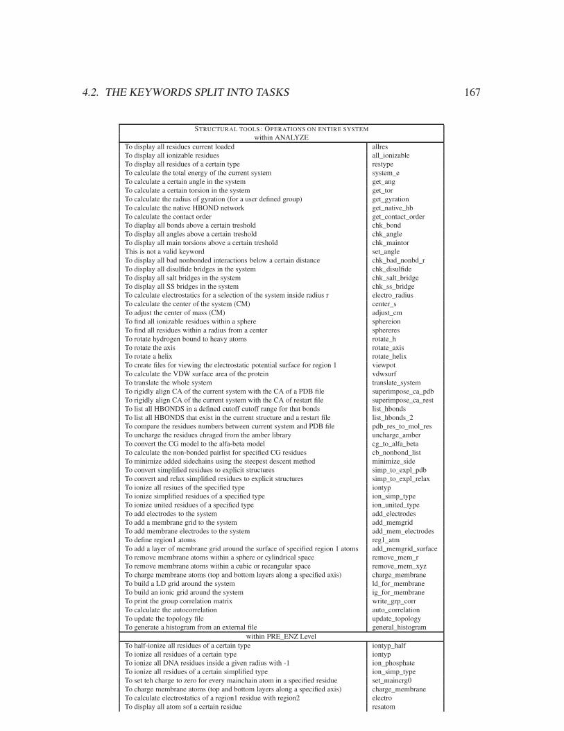
4.2. THE KEYWORDS SPLIT INTO TASKS 167
STRUCTURAL TOOLS: OPERATIONS ON ENTIRE SYSTEM
within ANALYZETo display all residues current loaded allresTo display all ionizable residues all_ionizableTo display all residues of a certain type restypeTo calculate the total energy of the current system system_eTo calculate a certain angle in the system get_angTo calculate a certain torsion in the system get_torTo calculate the radius of gyration (for a user defined group) get_gyrationTo calculate the native HBOND network get_native_hbTo calculate the contact order get_contact_orderTo diaplay all bonds above a certain treshold chk_bondTo display all angles above a certain treshold chk_angleTo display all main torsions above a certain treshold chk_maintorThis is not a valid keyword set_angleTo display all bad nonbonded interactions below a certain distance chk_bad_nonbd_rTo display all disulfide bridges in the system chk_disulfideTo display all salt bridges in the system chk_salt_bridgeTo display all SS bridges in the system chk_ss_bridgeTo calculate electrostatics for a selection of the system inside radius r electro_radiusTo calculate the center of the system (CM) center_sTo adjust the center of mass (CM) adjust_cmTo find all ionizable residues within a sphere sphereionTo find all residues within a radius from a center sphereresTo rotate hydrogen bound to heavy atoms rotate_hTo rotate the axis rotate_axisTo rotate a helix rotate_helixTo create files for viewing the electrostatic potential surface for region 1 viewpotTo calculate the VDW surface area of the protein vdwsurfTo translate the whole system translate_systemTo rigidly align CA of the current system with the CA of a PDB file superimpose_ca_pdbTo rigidly align CA of the current system with the CA of restart file superimpose_ca_restTo list all HBONDS in a defined cutoff cutoff range for that bonds list_hbondsTo list all HBONDS that exist in the current structure and a restart file list_hbonds_2To compare the residues numbers between current system and PDB file pdb_res_to_mol_resTo uncharge the residues chraged from the amber library uncharge_amberTo convert the CG model to the alfa-beta model cg_to_alfa_betaTo calculate the non-bonded pairlist for specified CG residues cb_nonbond_listTo minimize added sidechains using the steepest descent method minimize_sideTo convert simplified residues to explicit structures simp_to_expl_pdbTo convert and relax simplified residues to explicit structures simp_to_expl_relaxTo ionize all resiues of the specified type iontypTo ionize simplified residues of a specified type ion_simp_typeTo ionize united residues of a specified type ion_united_typeTo add electrodes to the system add_electrodesTo add a membrane grid to the system add_memgridTo add membrane electrodes to the system add_mem_electrodesTo define region1 atoms reg1_atmTo add a layer of membrane grid around the surface of specified region 1 atoms add_memgrid_surfaceTo remove membrane atoms within a sphere or cylindrical space remove_mem_rTo remove membrane atoms within a cubic or recangular space remove_mem_xyzTo charge membrane atoms (top and bottom layers along a specified axis) charge_membraneTo build a LD grid around the system ld_for_membraneTo build an ionic grid around the system ig_for_membraneTo print the group correlation matrix write_grp_corrTo calculate the autocorrelation auto_correlationTo update the topology file update_topologyTo generate a histogram from an external file general_histogram
within PRE_ENZ LevelTo half-ionize all residues of a certain type iontyp_halfTo ionize all residues of a certain type iontypTo ionize all DNA residues inside a given radius with -1 ion_phosphateTo ionize all residues of a certain simplified type ion_simp_typeTo set teh charge to zero for every mainchain atom in a specified residue set_maincrg0To charge membrane atoms (top and bottom layers along a specified axis) charge_membraneTo calculate electrostatics of a region1 residue with region2 electroTo display all atom sof a certain residue resatom

168 CHAPTER 4. INVERSE KEYWORDS
To display all bonds of a certain residue resbondwithin RELAX
To define all residues in region 2 region2_resTo calculate the protein energy of explicit and simple residues explicit_simpleTo minimize added sidechains using the steepest descent method minimize_sideTo minimize the main torsion in the protein minimize_main_torTo specify the minimum system energy for minimizing sidechains minimize_run_parmTo specify the center corrdinates for gyration calculations gyration_centerTo specify initial and final postions of the atom for the relax mapping relax_map_pmf_zTo relax with protein native-contact order constraint for simple system relax_map_contactTo relax with native HBOND constraints relax_map_native_hbTo calculate the protein contact order for explicit structures explicit_contactTo calculate electrostatics between substrate and the remainder of the system substrate_resTo specify the dielectric constant for substrate and sidechain atoms diele_sub_side
within ACTo define region 1 residues reg1_resTo define region 1 atoms reg1_atmTo write out the force on AC atoms check_fTo morph AC atoms during an AC calculation atom_B_shrink
within EVBTo monitor electrostatics between an EVB(s) atom and the system evb_grp_elecTo calculate electrostatics between an EVB an dprotein group evb_pro_grp_elecTo be used with other keyword evb_ts_II_0_atmTo calculate the LRA VDW contribution from each protein residue lra_grp_vdwTo calculate average electrostatics of each residue to each resonance state ave_elecTo calculate electrostatic contribution of main and sidechain atoms chain_ele_stateTo calculate VDW between evb and protein atoms vdw_evb_pTo delete an angle between EVB atoms kill_angTo add a new angle between EVB atoms (or atoms) add_angTo set a new angle between EVB atoms (or atoms) set_ang
Structural tools: Operations on selected residueswithin ANALYZE
To display all atom sof a certain residue resatomTo display all bonds of a certain residue resbondTo display all angles of a certain residue resangTo display all torsions of a certain residue restorTo display all improper torsions of a certain residue resitorTo specify the residue number and effective dielectric of a non-ionizable residue res_ion_vqTo display the distance between 2 atoms distatomTo calculate a certain angle in the system get_angTo calculate a certain torsion in the system get_torTo calculate the distance between 2 residues distresTo calculate the minimum distance between 2 residues (heavy atoms only!) minimum_distresTo calculate electrostatics for a pair of residues electro_resTo calculate the center of a given residue and to specify a new center and radius center_rTo find all atoms within a radius of a center sphereatmTo move a group of atoms move_atomsTo mutate a residue mutate_resTo mutate to a simplified residue (from simplified or explicit representation) mutate_simp_resTo mutate a residue to H2O mutate_res_to_h2oTo replace a solute molecule in the system replace_ligandTo return the residue number an atom belongs to whichresTo calculate the non-bonded pairlist for specified CG residues cb_nonbond_listTo convert simplified residues to explicit structures simp_to_expl_pdbTo convert and relax simplified residues to explicit structures simp_to_expl_relaxTo ionize all resiues of the specified type iontypTo ionize simplified residues of a specified type ion_simp_typeTo ionize united residues of a specified type ion_united_typeTo dock a ligand into a binding site dock_ligandTo add a new C-terminal residue add_res_at_endTo add a new N-terminal residue add_res_at_startTo insert a new residue at a specified position insert_resTo remove a residue at a specified position remove_res
within PRE_ENZTo ionize a certain residue ionresTo half-ionize a certain residue ionres_half

4.2. THE KEYWORDS SPLIT INTO TASKS 169
To half-ionize all residues of a certain type iontyp_halfTo unionize a certain residue unionresTo ionize all residues of a certain type iontypTo ionize all DNA residues inside a given radius with -1 ion_phosphateTo ionize all residues of a certain simplified type ion_simp_typeTo set the charge to zero for specified residues setcrg0To set teh charge to zero for every mainchain atom in a specified residue set_maincrg0To display all atom sof a certain residue resatomTo display all bonds of a certain residue resbond
Operations on atoms
To display the distance between 2 atoms distatomTo calculate a certain angle in the system get_angTo calculate a certain torsion in the system get_torTo calculate the distance between 2 sidechain atoms dist_cen_side_heavyTo change atom coordinates setxyzTo calculate electrostatics for a pair of atoms electro_atmTo calculate the center of a selection of atoms center_atomsTo find all atoms within a radius of a center sphereatmTo add a new bond between two atoms addbondTo display all bonds for an atom bonds_for_atomTo display all angles for an atom angles_for_atomTo remove a bond between atoms removebondTo render an atom dummy set_atom_dummyTo move a group of atoms move_atomsTo rotate an atom rotate_atomTo return the residue number an atom belongs to whichresTo add main chain atoms add_main_atomsTo add sidechain atoms add_sidechainTo define region1 atoms reg1_atmTo remove membrane atoms within a sphere or cylindrical space remove_mem_rTo remove membrane atoms within a cubic or recangular space remove_mem_xyzTo charge membrane atoms (top and bottom layers along a specified axis) charge_membrane
within PRE_ENZ LevelTo set a new charge for a specified atom setcrgTo change atom coordinates setxyzTo charge membrane atoms (top and bottom layers along a specified axis) charge_membraneTo use atomic coordinates from a restart for constraints rest_constrTo display all atom sof a certain residue resatomTo display all bonds of a certain residue resbond
Operations on bonds
To display all bonds of a certain residue resbondTo diaplay all bonds above a certain treshold chk_bondTo display all disulfide bridges in the system chk_disulfideTo display all salt bridges in the system chk_salt_bridgeTo display all SS bridges in the system chk_ss_bridgeTo add a new bond between two atoms addbondTo display all bonds for an atom bonds_for_atomTo display all angles for an atom angles_for_atomTo remove a bond between atoms removebondTo rotate hydrogen bound to heavy atoms rotate_hTo list all HBONDS in a defined cutoff cutoff range for that bonds list_hbondsTo list all HBONDS that exist in the current structure and a restart file list_hbonds_2
within PRE_ENZTo display all bonds of a certain residue resbond
Operations on angles
To display all angles of a certain residue resangTo calculate a certain angle in the system get_angTo display all angles above a certain treshold chk_angleTo display all angles for an atom angles_for_atom
Operations on torsions

170 CHAPTER 4. INVERSE KEYWORDS
To display all torsions of a certain residue restorTo display all improper torsions of a certain residue resitorTo calculate a certain torsion in the system get_torTo display all main torsions above a certain treshold chk_maintor
Operations on nonbonded interactions
To display all bad nonbonded interactions below a certain distance chk_bad_nonbd_rTo calculate electrostatics for a selection of the system inside radius r electro_radiusTo calculate electrostatics for a pair of residues electro_resTo calculate electrostatics for a pair of atoms electro_atmTo calculate the VDW surface area of the protein vdwsurf
Table of the Keywords PRE_ENZ LevelTo calculate electrostatics of a region1 residue with region2 electro
Operations for Coarse-grained modelling
To calculate the contact order get_contact_orderTo calculate the distance between 2 residues distresTo calculate the distance between 2 sidechain atoms dist_cen_side_heavyTo calculate the minimum distance between 2 residues (heavy atoms only!) minimum_distresTo rotate the axis rotate_axisTo rotate a helix rotate_helixTo rigidly align CA of the current system with the CA of a PDB file superimpose_ca_pdbTo rigidly align CA of the current system with the CA of restart file superimpose_ca_restTo convert the CG model to the alfa-beta model cg_to_alfa_betaTo calculate the non-bonded pairlist for specified CG residues cb_nonbond_listTo add main chain atoms add_main_atomsTo add sidechain atoms add_sidechainTo minimize added sidechains using the steepest descent method minimize_sideTo convert simplified residues to explicit structures simp_to_expl_pdbTo convert and relax simplified residues to explicit structures simp_to_expl_relaxTo relax with 2 PDB structures – Ask Dr. Chu here expl_pdb_2_relaxTo ionize simplified residues of a specified type ion_simp_typeTo ionize united residues of a specified type ion_united_typeTo add electrodes to the system add_electrodesTo add a membrane grid to the system add_memgridTo add membrane electrodes to the system add_mem_electrodesTo add a layer of membrane grid around the surface of specified region 1 atoms add_memgrid_surfaceTo remove membrane atoms within a sphere or cylindrical space remove_mem_rTo remove membrane atoms within a cubic or recangular space remove_mem_xyzTo charge membrane atoms (top and bottom layers along a specified axis) charge_membraneTo build a LD grid around the system ld_for_membraneTo build an ionic grid around the system ig_for_membrane
within PRE_ENZTo half-ionize a certain residue ionres_halfTo half-ionize all residues of a certain type iontyp_halfTo unionize a certain residue unionresTo ionize all DNA residues inside a given radius with -1 ion_phosphateTo ionize all residues of a certain simplified type ion_simp_typeTo set teh charge to zero for every mainchain atom in a specified residue set_maincrg0To charge membrane atoms (top and bottom layers along a specified axis) charge_membrane
MD settings: Steps and stepsizeTo set the number of steps NSTEPSTo define the stepsize [ps] STEPSIZETo define multiple stepsizes MULTI_STEPSIZETo change the stepsize during the run CH_STEPSIZETo specify the number of extra relaxation steps RELAX_1To specify that no automatic relaxation is performed no_auto_relaxTo define the stepsize for steepest descent STEEPEST_STEPSIZE
MD settings: Constraints
To specifying a start and end configuration for constraining pdb constraint_1_pdb

4.2. THE KEYWORDS SPLIT INTO TASKS 171
To define constraints for region 2 atoms CONSTRAINT_2To define constraints for water molecules CONSTRAINT_WTo define distance constraints for 2 sets of atoms CONSTRAINT_2DTo constraint the distance between a pair of atoms CONSTRAINT_PAIRTo define position constraints for an atom CONSTRAINT_POSTTo define a position constraints for atom and a point CONSTRAINT_RTo define an angular constraint CONSTRAINT_ANGTo define a torsional constraint CONSTRAINT_TORTo define a positional constraint on mainchain atoms CONSTRAINT_MAINTo define constraints for main torsions CONSTRAINT_MAINTORTo define positional constraints for a residue CONSTRAINT_RESTo define positional constraints for an atom CONSTRAINT_ATMTo define constraints for helix torsions and hbonds HELIX_CONSTRAINTTo constraint H atoms in their original positions H_CONSTRAINTTo use the SHAKE method for 2 atoms SHAKE_CONS_DISTTo define the SHAKE parameters SHAKE_PARAMETERTo use atomic coordinates from a restart for constraints rest_constrTo specify the distance and constraint force for region 1 atoms region1_plus_consTo freeze all atoms of a certain region FIX_REGIONTo freeze certain residues FIX_RESTo freeze certain atoms FIX_ATOMTo freeze the center of mass of region 1 atoms FIX_CENTER_OF_M_ITo freeze CA torsions FIX_CA_TORSIONSTo set the energy of fixed atoms constant (no update) NO_E_FIX_ATOMSTo keep the total energy of teh system constant CONSTANT_ETo specify constraints to go from initial to final structure pdb_2_consTo exclude atoms from the atoms included in pdb_2_cons pdb_2_free_atoms
MD settings: Cutoff radii
To define the radius for region2 REGION2A_RTo define the radius for the water solvent grid WATER_RTo define the distance of water to membrane atoms WATER_MEM_RTo specify the exclusion and water grid center coordinates ex_w_centerTo specify the distance and constraint force for region 1 atoms region1_plus_cons
MD settings: Temperature
To set the temperature TEMPERATURETo define the tolerance temperature TOLERANCE_TEMPTo define multiple steps in temperature MULTI_TEMPSTo define the target temperature in the xentroid run centroid_temp
MD settings: Solvation
To run in the gas phase GAS_PHASETo remove bulk water NO_BULKTo define the radius for the water solvent grid WATER_RTo define the distance of water to membrane atoms WATER_MEM_RTo define the langevin grid LANGEVIN_RTo specify the exclusion and water grid center coordinates ex_w_centerTo print waters around certain residues write_wat_from_resTo set the solvent solventTo switch on inductive forces induceTo specify the screen parameter in the induced dipole calculdation induce_screenTo set the dielectric constrant to screen electrostatic interaction electro_screenTo switch the calculation of the induced force on or off indforceTo switch on induction for ac atoms induce_ac_atomsTo specify LD with 2 solvents and user-defined reorganization energy langevin_chem_confTo specify the gamma parameter in LD simulations lan_dyn_gammaTo specify solevnt dipoles in LD simulations sol_evb_dipoleTo specify initial coordinates for each solevnt in sol_evb_dipole x_sol_0To specify the coupling of langevin dipole solvents sol_evb_coupleTo define the langevin solvent coupling strength qq_couple_factorTo specify the file for langevin solvent coordinates sol_file_nameTo request the use of implicit solvation exp_implicit_svTo specify the use of langevin dipoles for MD in explicit form expl_lgvn

172 CHAPTER 4. INVERSE KEYWORDS
To build a Langevin dipole grid LD_FOR_MEMBRANETo build an ionic grid IG_FOR_MEMBRANETo define a rectangular ionic grid around simplified system ig_rec_for_membraneTp specify a user-defined distance-dependent dielectric constant user_dielecTo calculate the macroscopic dielectric around a resiude MACRO_DIELECTRIC
MD settings: Monitoring and altering degrees of freedom
To set the frequency of updates of nonbonded interactions nbupdateTo calculate VDW interactions using defined parameters A & B p_pair_vdwTo calculate VDW interactions using defined parameters e and r p_pair_vdw_erTo switch off electrostatics between certain residues no_electro_pairTo assign dummy properties to an atom dummy_atomTo set the energy of fixed atoms constant (no update) NO_E_FIX_ATOMSTo set a new parameters for a certain angle ANGLE_PARMTo check all forces in the system CHECK_ALL_FTo monitor a certain angle in a simulation WRITE_ANGLETo define the frequency of angle monitoring ANGLE_WRITE_FQTo monitor a certain torsion in a simulation WRITE_TORSIONTo define the frequency of torsional monitoring TORSION_WRITE_FQTo monitor the velocity of atoms VELOCITY_ATOMSTo define the frequency of velocity monitoring VELOCITY_WRITE_FQTo define the frequency of the log files LOG_WRITE_FQTo define the frequency of the gap files GAP_WRITE_FQTo rigidly rotate a torsion and other atoms with it RIGID_ROT_TORTo generate a Ramachandran map RAMACHANDRAN_MAPTo keep the total energy of teh system constant CONSTANT_ETo set the replusion VDW parameter SET_VDW_PARM_ATo check all angles above a certain treshold CHECK_ANGLETo print the angles of water molecules WRITE_W_ANGLETo write a PDB file with angles for waters WRITE_PDB_W_ANGLETo keep the total energy of teh system constant CONSTANT_ETo specify the power parameter for LJ protein-protein NONBOND_LJ_ABTo specify the power parameter for LJ protein-protein (united atom) NONBOND_LJ_UHTo specify the added nonbonded interaction parameters for H-bonds hb_simp_gas_parmTo specify the added nonbonded interaction parameters for H-bonds hb_simp_gas_parm2To write out the average force on defined atoms write_ave_forceTo set the frequency for WRITE_AVE_FORCE write_ave_f_fqTo request the calculation of torsion normal modes for alfa_beta simple systems alfa_tor_nr_modesTo request the calculation of cartesian normal modes for CA and CB alfa_xyz_nr_modesTo calculate electrostatics between 2 residues ELECTRO_RESTo specify the scaling factor for VDW interactions between side and mainchain vdw_ms_scalingTo specify the calculation of VDW interactions (in certain cutoff distances) use_vdw_erTo specify a user-defined set of VDW repulsion parameters set_vdw_parm_aTo exclude atoms from the atoms included in pdb_2_cons pdb_2_free_atomsTo kill charges for atoms angled or bonded to region 1 atoms ba_crg_killTo specify printing of nonbonded interactions for each atom pair (regions 1 and 2) nonbond_grpTo specify the frequency of printing using nonbond_grp nonbond_e_w_fqTo print interactions between mainchains and sidechains write_main_side_eTo print the total HBONDS energy write_hb_e
MD settings: Minimization & Relaxation
To specify the number of extra relaxation steps RELAX_1To specify that no automatic relaxation no_auto_relaxTo optimize the protonation state of HIS residues OPT_HISTo minimize using steepest descent method STEEP_MINITo define the stepsize for steepest descent STEEPEST_STEPSIZETo minimize region 1 atoms using Newton Raphson NEWTON_RAPHSON_MINTo request minimizing the CA simple system using Newton-Raphson ca_tor_nr_minimizeTo request a Newton-Raphson minimization newton_raphson_min
MD settings: Coarse-grained modelling
To specify the exclusion and water grid center coordinates ex_w_centerTo specify the radius of gyration constraint of CA atoms gyration_consTo calculate the contact order GET_CONTACT_ORDER

4.2. THE KEYWORDS SPLIT INTO TASKS 173
To calculate contact order for an explicit structure EXPLICIT_CONTACTTo build a Langevin dipole grid LD_FOR_MEMBRANETo build an ionic grid IG_FOR_MEMBRANETo define a rectangular ionic grid around simplified system ig_rec_for_membraneTo request the calculation of torsion normal modes for alfa_beta simple systems alfa_tor_nr_modesTo request the calculation of cartesian normal modes for CA and CB alfa_xyz_nr_modesTo request minimizing the CA simple system using Newton-Raphson ca_tor_nr_minimizeTo calculate the contact order GET_CONTACT_ORDERTo calculate contact order for an explicit structure EXPLICIT_CONTACTTo calculate the radius of gyration GET_GYRATIONTo calculate the native hbonds GET_NATIVE_HBTo specify input data for calculating polarity in folding/unfolding simple_side_crg_fTo specify the library for calculating polarity in folding/unfolding simple_side_libTo specify the polar and nonpolar polarity for simple CG residues simp_res_polarityTo specify the dielectric constant and list of ionized sidechains sidechain_ionsTo define the strength and direction of external field EXTERNAL_FIELDTo define the polarizability value for membrane atoms (generated by molaris) polarizability_mem
MD settings: Entropy
To request a quasiharmonic estimate of the entropy QUASIH_ENTROPYTo specify the 2 states for the RR approach RR_STATETo specify the force constants for the RR approach RR_FORCETo specify the force constant for the quasiharmonic approach RR_QUASIHTo specify the restart files for a RR calculation rr_restartTo set several parameters for RR calculations rr_prepTo use Monte Carlo sampling instead of MD MC_DYNAMICSTo define a group of atoms for MC entropy correction MC_ENTROPY_ATOMSTo define the radius for the entropy calculation in MC MC_ENTROPY_RTo define a group of atoms for MC entropy correction MC_ENTROPY_ATOMSTo define the radius for the entropy calculation in MC MC_ENTROPY_R
MD settings: Visualization
To write out coordinates of specified residues in a abinary file MOVIE_COTo set the frequency of writing coordinates to the binary file MOVIE_FQ
within ANALYZETo enter the module to create a movie from a binary file VIEWMOVIETo specify the force constants for the RR approach RR_FORCETo specify the force constant for the quasiharmonic approach RR_QUASIHTo specify the restart files for a RR calculation rr_restartTo set several parameters for RR calculations rr_prepTo use Monte Carlo sampling instead of MD MC_DYNAMICSTo define a group of atoms for MC entropy correction MC_ENTROPY_ATOMSTo define the radius for the entropy calculation in MC MC_ENTROPY_RTo define a group of atoms for MC entropy correction MC_ENTROPY_ATOMSTo define the radius for the entropy calculation in MC MC_ENTROPY_R

174 CHAPTER 4. INVERSE KEYWORDS

Chapter 5
Appendices
5.1 List of Demos
5.1.1 Demo an_total
Analyze the system and obtain divers info from it.
5.1.2 Demo ez_relax
Relaxation of a protein with molecular dynamics.
5.1.3 Demo ez_EVBgasphase
5.1.4 Demo ez_EVB
EVB calculation for the reaction catalysed by ubtilisin in water and in the protein. The results are written in $OUT_DIR/evb_subwatand $OUT_DIR/evb_sub, respectively. Note that the gap files generated by this demo, which correspond to the energy values for eachframe in the free energy perturbation (FEP) calculation are located in $OUT_DIR/*. Mapping of those files is done by the programxmap which is provided with MOLARIS.
175

176 CHAPTER 5. APPENDICES
5.1.5 Demo ez_EVBcentroid
5.1.6 Demo ez_EVBadiabgasphase
5.1.7 Demo ez_EVBadiab
5.1.8 Demo ez_EVBnonequilibrium
5.1.9 Demo ez_PMF
5.1.10 Demo ez_AC
5.1.11 Demo ez_RRA
5.1.12 Demo pl_solvpdld
5.1.13 Demo pl_solvfep
5.1.14 Demo pl_aipdld
5.1.15 Demo pl_bindpdld
5.1.16 Demo pl_pkapdldpKacalculation of a residue in a protein. The results are written in $OUT_DIR/bpti_pka.
5.1.17 Demo pl_pkafep
5.1.18 Demo pl_redoxpdld
5.1.19 Demo pl_redoxfep
5.1.20 Demo pl_logp
5.1.21 Demo pl_titraph0
5.1.22 Demo pl_evbpdld

Bibliography
[1] A. Warshel, Computer Modeling of Chemical Reactions in Enzymes and Solutions. New York: John Wiley & Sons, 1991.
[2] A. Warshel and S. T. Russell, “Calculations of electrostatic interactions in biological systems and in solutions,” Q. Rev. Biophys.,vol. 17, pp. 283–421, 1984.
[3] S. C. L. Kamerlin, S. Vicatos, A. Dryga, and A. Warshel, “Coarse-grained (multiscale) simulations in studies of biophysical andchemical systems.,” ARPC, vol. 62, pp. 41–64.
[4] J. Villà and A. Warshel, “Energetics and dynamics of enzymatic reactions,” J. Phys. Chem. B, vol. 105, pp. 7887–7907, 2001.
[5] S. C. L. Kamerlin, M. Haranczyk, and A. Warshel, “Progress in ab initio qm/mm free energy simulations of electrostatic energiesin proteins: Accelerated qm/mm studies of pka, redox reactions and solvation free energies.,” JPCB, vol. 113, no. 5, pp. 1253–1272.
[6] F. S. Lee, Z. T. Chu, M. B. Bolger, and A. Warshel, “Calculations of antibody-antigen interactions: Microscopic and semi-microscopic evaluation of the free energies of binding of phosphorylcholine analogs to mcpc603,” Prot. Eng., vol. 5, pp. 215–228,1992.
[7] A. Warshel, F. Sussman, and G. King, “Free energy of charges in solvated proteins: Microscopic calculations using a reversiblecharging process,” Biochemistry, vol. 25, p. 8368, 1986.
[8] F. S. Lee and A. Warshel, “A local reaction field method for fast evaluation of long-range electrostatic interactions in molecularsimulations,” J. Chem. Phys., vol. 97, no. 5, pp. 3100–3107, 1992.
[9] Y. Y. Sham and A. Warshel, “The surface constrained all atom model provides size independent results in calculations of hydrationfree energies,” J. Chem. Phys., vol. 109, pp. 7940–7944, 1998.
[10] J. Åqvist, “Calculation of absolute binding free energies for charged ligands and effects of long-range electrostatic interactions,”J. Comput. Chem., vol. 17, no. 14, p. 1587, 1996.
[11] J. Warwicker and H. C. Watson, “Calculation of the electric potential in the active site cleft due to alpha-helix dipoles,” J. Mol.
Biol., vol. 157, pp. 671–9, 1982.
[12] K. A. Sharp and B. Honig, “Electrostatic interactions in macromolecules: Theory and applications,” Ann. Rev. Biophys. Biophys.
Chem., vol. 19, pp. 301–332, 1990.
[13] F. S. Lee, Z. T. Chu, and A. Warshel, “Microscopic and semimicroscopic calculations of electrostatic energies in proteins by thepolaris and enzymix programs,” J. Comput. Chem., vol. 14, pp. 161–185, 1993.
[14] A. Papazyan and A. Warshel, “Effect of solvent discreteness on solvation,” J. Phys. Chem. B, vol. 102, pp. 5248–5357, 1998.
[15] J. B. Hendrickson J. Am. Chem. Soc., vol. 83, p. 5437, 1961.
[16] U. Burkert and N. Allinger, Molecular Mechanics. Washington D. C.: American Chemical Society, 1982.
[17] S. Lifson and A. Warshel, “A consistent force field for calculation on conformations, vibrational spectra and enthalpies of cy-cloalkanes and n-alkane molecules,” J. Chem. Phys., vol. 49, p. 5116, 1968.
[18] M. Levitt and S. Lifson J. Mol. Biol., vol. 46, pp. 269–279, 1969.
[19] P. Kollman, “Free energy calculations: Applications to chemical and biochemical phenomena,” Chem. Rev., vol. 93, no. 7,pp. 2395–2417, 1993.
[20] M. P. Allen and D. J. Tildesley, Computer Simulation of Liquids. Oxford: Oxford University Press, 1987.
177

178 BIBLIOGRAPHY
[21] G. King and A. Warshel, “A surface constrained all-atom solvent model for effective simulations of polar solutions,” J. Chem.
Phys., vol. 91, no. 6, pp. 3647–3661, 1989.
[22] S. Miertus, E. Scrocco, and J. Tomasi, “Electrostatic interaction of a solute with a continuum. a direct utilization of ab initiomolecular potentials for the prevision of solvent effects,” J. Chem. Phys., vol. 55, pp. 117–129, 1981.
[23] R. Fletcher, Practical Methods of Optimization. New York: Wiley, 1980.
[24] A. Warshel, “Bicycle-pedal model for the first step in the vision process,” Nature, vol. 260, pp. 679–683, 1976.
[25] J. A. McCammon, B. R. Gelin, and M. Karplus Nature, vol. 267, p. 585, 1977.
[26] M. Levitt, “Molecular dynamics of native proteins ii. analysis and nature of motion,” J. Mol. Biol., vol. 168, pp. 621–657, 1983.
[27] W. F. van Gunsteren and A. E. Mark, “On the interpretation of biochemical data by molecular dynamics simulation,” Eur. J.
Biochem., vol. 204, p. 947, 1992.
[28] D. A. McQuarrie, Statistical Mechanics. New York: Harper and Row, 1976.
[29] R. W. Zwanzig, “High-temperature equation of state by a perturbation method. i. nonpolar gases,” J. Chem. Phys., vol. 22,p. 1420, 1954.
[30] J. P. Valleau and G. M. Torrie, Modern Theoretical Chemistry, Vol. 5, vol. 5 of A Guide to Monte Carlo for Statistical Mechanics.
2. Byways. New York: Plenum Press, 1977.
[31] A. Warshel and J. Åqvist, “Electrostatic energy and macromolecular function,” Ann. Rev. Biophys. Chem., vol. 20, p. 267, 1991.
[32] A. Warshel, “Dynamics of reactions in polar solvents. semiclassical trajectory studies of electron-transfer and proton-transferreactions,” J. Phys. Chem., vol. 86, no. 12, pp. 2218–2224, 1982.
[33] G. King and A. Warshel, “Investigation of the free energy functions for electron transfer reactions,” J. Chem. Phys., vol. 93,pp. 8682–8692, 1990.
[34] Y. Sham, Z. T. Chu, H. Tao, and A. Warshel, “Examining Methods for Calculations of Binding Free Energies: LRA, LIE, PDLD-LRA and PDLD/S-LRA Calculations of Ligands Binding to an HIV Protease,” Proteins: Struct. Func. Gen., vol. 39, pp. 393–407,2000.
[35] J.-K. Hwang and A. Warshel, “Microscopic examination of free energy relationships for electron transfer in polar solvents,” J.
Am. Chem. Soc., vol. 109, pp. 715–720, 1987.
[36] R. A. Kuharski, J. S. Bader, D. Chandler, M. Sprik, M. L. Klein, and R. W. Impey, “Molecular model for aqueous ferrous ferricelectron transfer,” J. Chem. Phys., vol. 89, pp. 3248–3257, 1988.
[37] G. Hummer and A. Szabo, “Calculation of free-energy differences from computer simulations of initial and final states,” J. Chem.
Phys., vol. 105, pp. 2004–2010, 1996.
[38] S. Kuwajima and A. Warshel, “The extended ewald method: A general treatment of long-range electrostatic interactions inmicroscopic simulations,” J. Chem. Phys., vol. 89, p. 3751, 1988.
[39] A. Warshel and R. Weiss, “An empirical valence bond approach for comparing reactions in solutions and in enzymes,” J. Am.
Chem. Soc., vol. 102, no. 20, pp. 6218–6226, 1980.
[40] J. Åqvist and A. Warshel, “Simulation of enzyme reactions using valence bond force fields and other hybrid quantum/classicalapproaches,” Chem. Rev., vol. 93, pp. 2523–2544, 1993.
[41] A. Warshel, F. Sussman, and J.-K. Hwang, “Evaluation of catalytic free energies in genetically modified proteins,” J. Mol. Biol.,vol. 201, pp. 139–159, 1988.
[42] J.-K. Hwang, G. King, S. Creighton, and A. Warshel, “Simulation of Free Energy Relationships and Dynamics of SN2 Reactionsin Aqueous Solution,” J. Am. Chem. Soc., vol. 110, no. 16, pp. 5297–5311, 1988.
[43] A. Warshel and M. Levitt, “Theoretical studies of enzymatic reactions: Dielectric, electrostatic and steric stabilization of thecarbonium ion in the reaction of lysozyme,” J. Mol. Biol., vol. 103, pp. 227–249, 1976.
[44] V. Théry, D. Rinaldi, B. Rivail, J. L. Maigret, and G. G. Ferenczy, “Quantum mechanical computations on very large systems:The local self-consistent field method,” J. Comput. Chem., vol. 15, pp. 269–282, 1994.

BIBLIOGRAPHY 179
[45] Y. K. Zhang, H. Y. Liu, and W. T. Yang, “Free energy calculation on enzyme reactions with an efficient iterative procedure todetermine minimum energy paths on a combined ab initio qm/mm potential energy surface,” J. Chem. Phys., vol. 112, pp. 3483–3492, 2000.
[46] J. Gao, “Hybrid quantum and molecular mecanical simulations: an alternative avenue to solvent effects in organic chemistry,”Acc. Chem. Res., vol. 29, pp. 298–305, 1996.
[47] D. Bakowies and W. Thiel, “Hybrid models for combined quantum mechanical and molecular mechanical approaches,” J. Phys.
Chem., vol. 100, pp. 10580–10594, 1996.
[48] M. Field, P. Bash, and M. Karplus, “A combined quantum mechanical and molecular mechanical potential for molecular dynamicssimulations,” J. Comput. Chem., vol. 11, no. 6, p. 700, 1990.
[49] R. Friesner and M. D. Beachy, “Quantum mechanical calculations on biological systems,” Curr. Opin. Struct. Biol., vol. 8,pp. 257–262, 1998.
[50] G. Monard and K. M. Merz, “Combined quantum mechanical/molecular mechanical methodologies applied to biomolecularsystems,” Acc. Chem. Res., vol. 32, no. 10, pp. 904–911, 1999.
[51] M. García-Viloca, A. Gonzàlez-Lafont, and J. M. Lluch, “A qm/mm study of the racemization of vinylglycolate catalyzed bymandelate racemase enzyme,” J. Am. Chem. Soc., vol. 123, pp. 709–721, 2001.
[52] S. Martí, J. Andrés, V. Moliner, E. Silla, I. Tuñon, and J. Bertrán, “Transition structure selectivity in enzyme catalysis: a qm/mmstudy of chorismate mutase,” Theor. Chem. Acc., vol. 3, pp. 207–212, 2001.
[53] M. A. Cunningham, L. L. Ho, D. T. Nguyen, R. E. Gillilan, and P. A. Bash, “Simulation of the enzyme reaction mechanism ofmalate dehydrogenase,” Biochemistry, vol. 36, pp. 4800–4816, 1997.
[54] N. Wu, Y. Mo, J. Gao, and E. Pai Proc. Natl. Acad. Sci. USA, vol. 97, pp. 2017–2022, 2000.
[55] J. Bentzien, R. Muller, J. Florián, and A. Warshel, “Hybrid ab initio quantum mechanics/molecular mechanics calculations of freeenergy surfaces for enzymatic reactions: The nucleophilic attack in subtilisin,” J. Phys. Chem. B, vol. 102, no. 12, pp. 2293–2301,1998.
[56] A. Warshel and Z. T. Chu, “Nature of the surface crossing process in bacteriorhodopsin: Computer simulations of the quantumdynamics of the primary photochemical event,” J. Phys. Chem. B, vol. 105, pp. 9857–9871, 2001.
[57] M. Štrajbl, Y. Y. Sham, J. Villà, Z. T. Chu, and A. Warshel, “Calculations of activation entropies of chemical reactions in solution,”J. Phys. Chem. B, vol. 104, pp. 4578 –4584, 2000.
[58] N. Singh and A. Warshel, “Toward accurate microscopic calculation of solvation entropies: Extending the restraint releaseapproach to studies of solvation effects,” The Journal of Physical Chemistry B, vol. 113, no. 20, pp. 7372–7382, 2009. PMID:19402609.
[59] N. Singh and A. Warshel, “Absolute binding free energy calculations: On the accuracy of computational scoring of protein-ligandinteractions,” PROTEINS, vol. 78, no. 7, pp. 1705–1723, 2010.
[60] N. Singh and A. Warshel, “A comprehensive examination of the contributions to the binding entropy of protein£ligand com-plexes,” Proteins: Structure, Function, and Bioinformatics, vol. 78, no. 7, pp. 1724–1735, 2010.
[61] J. Florián and A. Warshel, “Langevin dipoles model for ab initio calculations of chemical processes in solution: Parameterizationand application to hydration free energies of neutral and ionic solutes, and conformational analysis in aqueous solution,” J. Phys.
Chem. B, vol. 101, no. 28, pp. 5583–5595, 1997.
[62] J. Florián and A. Warshel, “Chemsol,” 1997.
[63] J. Florián and A. Warshel, “Calculations of hydration entropies of hydrophobic, polar, and ionic solutes in the framework of thelangevin dipoles solvation model,” J. Phys. Chem. B, vol. 103, pp. 10282–10288, 1999.
[64] A. Warshel, S. T. Russell, and A. K. Churg, “Macroscopic models for studies of electrostatic interactions in proteins: Limitationsand applicability,” Proc. Natl. Acad. Sci. USA, vol. 81, p. 4785, 1984.
[65] Y. Y. Sham, Z. T. Chu, and A. Warshel, “Consistent calculations of pka’s of ionizable residues in proteins: Semi-microscopic andmacroscopic approaches,” J. Phys. Chem. B, vol. 101, no. 22, pp. 4458–4472, 1997.
[66] A. Warshel, M. Štrajbl, J. Villà, and J. Florián, “Remarkable rate enhancement of orotidine 5’-monophosphate decarboxylase isdue to transition state stabilization rather than to ground state destabilization,” Biochemistry, vol. 39, pp. 14728–14738, 2000.

180 BIBLIOGRAPHY
[67] C. N. Schutz and A. Warshel, “What are the dielectric,” Proteins: Struct. Func. Gen.
[68] M. Štrajbl, J. Florián, and A. Warshel, “Ab initio evaluation of the potential surface for general base- catalyzed methanolysis offormamide: A reference solution reaction for studies of serine proteases,” J. Am. Chem. Soc., vol. 122, pp. 5354–5366, 2000.
[69] M. Štrajbl, J. Florián, and A. Warshel J. Phys. Chem. B, 2001.
[70] R. Stanton, M. Peräkylä, D. Bakowies, and P. A. Kollman, “Combined ab initio and free energy calculations to study reactions inenzymes and solution: Amide hydrolysis in trypsin and aqueous solution,” J. Am. Chem. Soc., vol. 120, pp. 3448–3457, 1998.
[71] A. Warshel and Z. T. Chu, “Calculations of solvation free energies in chemistry and biology,” in ACS Symposium Series: Structure
and Reactivity in Aqueous Solution. Characterization of Chemical and Biological Systems (D. G. C. Truhlar and C. J., eds.),pp. 72–93, Washington, D. C.: ACS, 1994.
[72] R. Langen, G. Brayer, A. Berghuis, G. McLendon, F. Sherman, and A. Warshel, “Effect of the asn52→ile mutation on the redoxpotential of yeast cytochrome c,” J. Mol. Biol., vol. 224, pp. 589–600, 1992.
[73] M. F. Perutz, “Electrostatic effects in proteins,” Science, vol. 201, p. 1187, 1978.
[74] G. King, F. S. Lee, and A. Warshel, “Microscopic simulations of macroscopic dielectric constants of solvated proteins,” J. Chem.
Phys., vol. 95, pp. 4366–4377, 1991.
[75] J. Åqvist, H. Luecke, F. A. Quiocho, and A. Warshel, “Dipoles localized at helix termini of proteins stabilize charges,” Proc.
Natl. Acad. Sci. USA, vol. 88, p. 2026, 1991.
[76] A. Warshel, P. K. Sharma, M. Kato, and W. W. Parson, “Modeling electrostatic effects in proteins.,” BBA, vol. 1764, no. 11,pp. 1647–1676, 2006.
[77] M. Levitt and A. Warshel, “Computer simulations of protein folding,” Nature, vol. 253, pp. 694–698, 1975.
[78] A. Warshel and M. Levitt, “Folding and stability of helical proteins: Carp myogen,” J. Mol. Biol., vol. 106, pp. 421–437, 1976.
[79] H. Taketomi, Y. Ueda, and N. Go Int. J. Peptide Res., vol. 7, no. 3, pp. 235–252, 1975.
[80] S. C. Kamerlin, S. Vicatos, A. Dryga, and A. Warshel, “Coarse-grained (multiscale) simulations in studies of biophysical andchemical systems,” Ann Rev Phys Chem, vol. 62, pp. 41–64, 2011.
[81] H. Nymeyer, A. E. García, and J. N. Onuchic, “Folding funnels and frustration in off-lattice minimalist protein landscapes,” Proc.
Natl. Acad. Sci. U. S. A., vol. 95, no. 11, pp. 5921–5928, 1998.
[82] P. G. Wolynes, “Recent sucesses of the energy lanscape theory of protein folding and function„”
[83] K. A. Dill, “Dominant forces in protein folding.,” Biochemistry, vol. 29, no. 31, pp. 7133–7155, 1990.
[84] D. A. Hinds and M. Levitt, “A lattice model for protein structure prediction at low resolution.,” Proc. Natl. Acad. Sci. U.S.A.,vol. 89, pp. 2536–2540, 1992.
[85] E. Shakhnovich, V. Abkevich, and O. Ptitsyn, “Conserved residues and the mechanism of protein folding.,” NAT, vol. 379,no. 6560, pp. 96–98, 1996.
[86] A. Heath, L. Kavraki, and C. Clementi, “From coarse-grain to all-atom: Toward multiscale analysis of protein landscapes.,”Proteins, vol. 68, pp. 646–661, 2007.
[87] C. Guardiani, R. Livi, and F. Cecconi, “Coarse grained modeling and approaches to protein folding,” Current bioinformatics,vol. 5, no. 3, pp. 217–240, 2010.
[88] V. Tozzini, “Coarse-grained models for proteins,” Current opinion in structural biology, vol. 15, no. 2, pp. 144–150, 2005.
[89] C. Wu and J. Shea, “Coarse-grained models for protein aggregation,” Current opinion in structural biology, vol. 21, no. 2,pp. 209–220, 2011.
[90] S. J. Marrink, H. J. Risselada, S. Yefimov, D. P. Tieleman, and A. H. de Vries, “The martini force field: Coarse grained modelfor biomolecular simulations,” Journal of Physical Chemistry B, vol. 111, no. 27, pp. 7812–7824, 2007.
[91] G. A. Voth, “Multiscale simulation of multiprotein assemblies: The challenges of ultra-coarse-graining,” Biophys J, vol. 104,no. 2, pp. 376a–376a, 2013.

BIBLIOGRAPHY 181
[92] C. Hyeon and D. Thirumalai, “Capturing the essence of folding and functions of biomolecules using coarse-grained models,” Nat
Commun, no. 2, 2011.
[93] A. Dryga, S. Chakrabarty, S. Vicatos, and A. Warshel, “Realistic simulation of the activation of voltage-gated ion channels,”PNAS, vol. 109, no. 9, pp. 3335–3340, 2012.
[94] B. M. Messer, M. Roca, Z. T. Chu, S. Vicatos, A. V. Kilshtain, and A. Warshel, “Multiscale simulations of protein landscapes:Using coarse-grained models as reference potentials to full explicit models,” Proteins, vol. 78, pp. 1212–1227, 2010.
[95] A. Warshel, M. Levitt, and S. Lifson, “Consistent Force Field for Calculation of Vibrational Spectra and Conformations of SomeAmides and Lactam Rings,” J. Mol. Spect., vol. 33, p. 84, 1970.
[96] Z. Fan, J.-K. Hwang, and W. A., “Using simplified protein representation as a reference potential for all-atom calculations offolding free energy.,” Theor Chem Acc, vol. 103, no. 1, pp. 77–80, 1999.
[97] N. V. Plotnikov and A. Warshel, “Exploring, refining and validating the paradynamics qm/mm sampling,” J Phys Chem B,vol. 116, no. 34, pp. 10342–10356, 2012.
[98] N. V. Plotnikov, S. C. Kamerlin, and W. A., “Paradynamics: An effective and reliable model for ab initio qm/mm free-energycalculations and related tasks,” J Phys Chem B, vol. 115, no. 24, pp. 7950–7962, 2011.
[99] S. Izvekov and G. A. Voth, “A multiscale coarse-graining method for biomolecular systems,” Journal of Physical Chemistry B,vol. 109, no. 7, pp. 2469–2473, 2005.
[100] A. Warshel and S. Lifson, “Consistent Force Field Calculations. II. Crystal Structure, Sublimation Energies, Molecular andLattice Vibrations, Molecular Conformations and Enthalpies of Alkanes,” J. Chem. Phys., vol. 53, p. 582, 1970.
[101] M. Roca, B. Messer, and A. Warshel, “Electrostatic contributions to protein stability and folding energy.,” FEBS Lett., vol. 581,no. 10, pp. 2065–2071, 2007.
[102] S. Vicatos, M. Roca, and A. Warshel, “Effective approach for caluclations of absolute stability of proteins using focused dielectricconstants.,” Proteins, vol. 77, no. 3, pp. 670–684, 2009.
[103] S. Vicatos, A. Rychkova, S. Mukherjee, and A. War shel, “An effective coarse-grained model for biological simulations: Recentrefinements and validations,” Proteins: Structure, Function, and Bioinformatics, vol. 82, no. 7, pp. 1168–1185, 2014.
[104] A. Rychkova, S. Vicatos, and A. Warshel, “On the energetics of translocon-assisted insertion of charged transmembrane helicesinto membranes,” PNAS, vol. 107, no. 41, pp. 17598–17603, 2010.
[105] A. Dryga, S. Chakrabarty, S. Vicatos, and A. Warshel, “Coarse grained model for exploring voltage dependent ion channels,”BBA, vol. 1818, no. 2, pp. 303–317, 2012.
[106] B. J. Klein and G. R. Pack, “Calculations of the spatial distribution of charge density in the environment of dna,” Biopolymers,vol. 22, pp. 2331–52, 1983.
[107] J. Åqvist, M. Fothergill, and A. Warshel, “Computer simulation of the co2/hco-3 interconversion step in human carbonic anhy-drase i,” J. Am. Chem. Soc., vol. 115, pp. 631–635, 1993.
[108] R. M. Levy and E. Gallicchio, “Computer simulations with explicit solvent: Recent progress in the thermodynamic decompositionof free energies and in modeling electrostatic effects,” Annu. Rev. Phys. Chem., vol. 49, pp. 531–567, 1998.
[109] A. Warshel, “Correlation between structure and efficiency of light-induced proton pumps,” in Methods in Enzymology (L. Packer,ed.), vol. 127, pp. 578–587, London: Academic Press Inc., 1986.
[110] A. Warshel, “On the origin of the red shift of the absorption spectra of aggregated chlorophylls,” J. Am. Chem. Soc., vol. 101,p. 774, 1979.
[111] S. K. S. R. G. M. R. Y. A. S. Honig, B., “On the calculation of pkas in proteins,” Proteins: Struct. Func. Gen., vol. 15, pp. 252–265, 1993.
[112] W. W. Parson, Z. T. Chu, and A. Warshel, “Electrostatic control of charge separation in bacterial photosynthesis,” Biochim.
Biophys. Acta, vol. 1017, p. 251, 1990.
[113] R. Langen, G. M. Jensen, U. Jacob, P. J. Stephens, and A. Warshel, “Protein control of iron-sulfur cluster redox potentials,” J.
Biol. Chem., vol. 267, p. 25625, 1992.
[114] P. J. Stephens, D. R. Jollie, and A. Warshel, “Protein control of redox potentials of iron-sulfur proteins,” Chem. Rev., vol. 96,p. 2491, 1996.

182 BIBLIOGRAPHY
[115] I. Muegge, P. X. Qi, A. J. Wand, Z. T. Chu, and A. Warshel, “The reorganization energy of cytochrome c revisited,” J. Phys.
Chem. B, vol. 101, pp. 825–836, 1997.
[116] H. Tao, Z. T. Chu, and A. Warshel, “Quantitative studies of ligand-receptor interactions: a rapid evaluation of binding freeenergies of endothiapepsin to its inhibitors,” in Pacific Symposium on Biocomputing (L. H. Klein and T., eds.), pp. 752–755,Singapore: World Scientific Press, 1996.
[117] J. Åqvist, C. Medina, and J.-E. Samuelsson, “A new method for predicting binding affinity in computer-aided drug design,” Prot.
Eng., vol. 7, pp. 385–391, 1994.
[118] J. Marelius, M. Graffernorgberg, T. Hansson, A. Hallberg, and J. Åqvist, “Computation of affinity and selectivity - binding of2,4-diaminopteridine and 2,4-diaminoquinazoline inhibitors to dihydrofolate reductases,” J. of Comp.-Aided Mol. Des., vol. 12,pp. 119–131, 1998.
[119] I. Muegge, T. Schweins, R. Langen, and A. Warshel, “Electrostatic control of gtp and gdp binding in the oncoprotein p21 ras,”Structure, vol. 4, pp. 475–489, 1996.
[120] I. Muegge, H. Tao, and A. Warshel, “A fast estimate of electrostatic group contributions to the free energy of protein inhibitorbinding,” Prot. Eng., vol. 10, no. 12, pp. 1363–1372, 1998.
[121] J. Åqvist and A. Warshel, “Energetics of ion permeation through membrane channels. solvation of na+ by gramicidin a,” Biophys.
J., vol. 56, p. 171, 1989.
[122] Y. Sham, I. Muegge, and A. Warshel, “Simulating proton translocations in proteins: Probing proton transfer pathways in therhodobacter sphaeroides reaction center,” Proteins: Struct. Func. Gen., vol. 36, pp. 484–500, 1999.
[123] J. Åqvist and A. Warshel, “Consistent calculations of electrostatic free energies in membrane channels. the solvation of na+ bythe gramicidin channel,” Comments Mol. cell. Biophys., vol. 6, p. 91, 1989.