Theorem proving -...

1

Theorem provingFormal MethodsLecture 8

Farn Wang Department of Electrical EngineeringNational Taiwan University

Theorem Proving: Historical Perspective

Theorem proving (or automated deduction) = logical deduction performed by machineAt the intersection of several areas

Mathematics: original motivation and techniquesLogic: the framework and the meta-reasoning techniques

2

Theorem proving

Prove that an implementation satisfies a specification by mathematical reasoning

implement Spec

implication

equivalenceor

Theorem proving

Implementation and specification expressed as formulas in a formal logicRequired relationship (logical equivalence/logical implication) described as a theorem to be proven within the context of a proof calculusA proof system:

A set of axioms and inference rules (simplification, rewriting, induction, etc.)

3

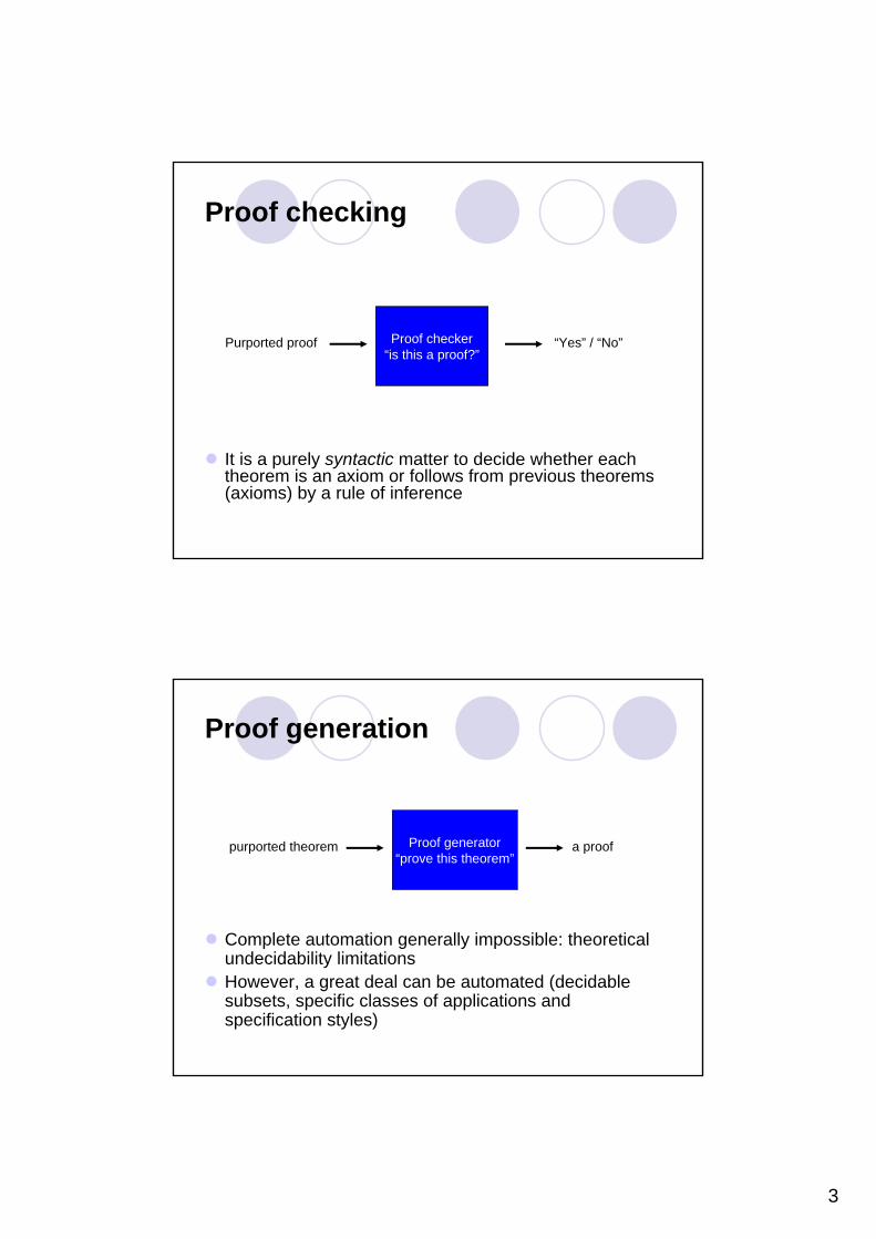
Proof checking

It is a purely syntactic matter to decide whether each theorem is an axiom or follows from previous theorems (axioms) by a rule of inference

Proof checker“is this a proof?”

Purported proof “Yes” / “No”

Proof generation

Complete automation generally impossible: theoretical undecidability limitationsHowever, a great deal can be automated (decidable subsets, specific classes of applications and specification styles)

Proof generator“prove this theorem”

purported theorem a proof

4

Applications

Hardware and software verification (or debugging)Automatic program synthesis from specificationsDiscovery of proofs of conjectures

A conjecture of Tarskiwas proved by machine (1996)There are effective geometry theorem provers

Program Verification

Fact: mechanical verification of software would improve software productivity, reliability, efficiencyFact: such systems are still in experimental stage

After 40 years !Research has revealed formidable obstaclesMany believe that program verification is extremely difficult

5

Program Verification

Fact:Verification is done with respect to a specificationIs the specification simpler than the program ?What if the specification is not right ?

Answer:Developing specifications is hardStill redundancy exposes many bugs as inconsistenciesWe are interested in partial specifications

An index is within bounds, a lock is released…

Programs, Theorems. Axiomatic Semantics

Consists of:A language for writing specifications about programsRules for establishing when specifications hold

Typical specifications:During the execution, only non-null pointers are dereferencedThis program terminates with x = 0

Partial vs. total correctness specificationsSafety vs. liveness propertiesUsually focus on safety (partial correctness)

6

Specification Languages

Must be easy to use and expressive (conflicting needs)

Most often only expressiveTypically they are extensions of first-order logic

Although higher-order or modal logics are also usedWe focus here on state-based specifications (safety)

State = values of variables + contents of heap (+ past state)

Not allowed: “variable x is live”, “lock L will be released”, “there is no correlation between the values of x and y”

A Specification Language

We’ll use a fragment of first-order logic:Formulas P ::= A | true | false | P1∧P2| P1∨P2| ¬P | ∀x.PAtoms A ::= E1≤E2| E1= E2| f(A1,…,An) | …

※ All boolean expressions from our language are atomsCan have an arbitrary collection of predicate symbols

reachable(E1,E2) - list cell E2 is reachable from E1sorted(a, L, H) - array a is sorted between L and Hptr(E,T) - expression E denotes a pointer to TE : ptr(T) - same in a different notation

An assertion can hold or not in a given stateEquivalently, an assertion denotes a set of states

7

Program Verification Using Hoare’s Logic

Hoare Triples

Partial correctness: { P } s { Q }When you start s in any state that satisfies PIf the execution of s terminatesIt does so in a state that satisfies Q

Total correctness: [ P ] s [ Q ]When you start sin any state that satisfies PThe execution of s terminates andIt does so in a state that satisfies Q

Defined inductively on the structure of statements

8

Hoare Rules

Assignmentsy:=t

CompositionS1; S2

If-then-elseif e the S1 else S2

While while e do S

Consequence

Greatest common divisor

{x1>0 ∧ x2>0}y1:=x1;y2:=x2;while ¬(y1=y2) do

if y1>y2 then y1:=y1-y2else y2:=y2-y1

{y1=gcd(x1,x2)}

9

Why it works?

Suppose that y1,y2 are both positive integers.If y1>y2 then gcd(y1,y2)=gcd(y1-y2,y2)If y2>y1 then gcd(y1,y2)=gcd(y1,y2-y1)If y1-y2 then gcd(y1,y2)=y1=y2

Hoare Rules: Assignment

General rule:{p[t/y]} y:=t {p}

Examples: {y+5=10} y:=y+5 {y=10}{y+y<z} x:=y {x+y<z}{2*(y+5)>20} y:=2*(y+5) {y>20}

Justification: write p with y’ instead of y, and add the conjunct y’=t. Next, eliminate y’ by replacing y’ by t.

10

Hoare Rules: Assignment

{p} y:=t {?}Strategy: write p and the conjunct y=t, where y’ replaces y in both p and t. Eliminate y’.

Example:{y>5} y:=2*(y+5) {?}

{p} y:=t {∃y’ (p[y’/y] t[y’/y]=y)}y’>5 y=2*(y’+5) → y>20

∧∧

Hoare Rules: Composition

General rule:{p} S1 {r}, {r} S2 {q} → {p} S1;S2 {q}

Example: if the antecedents are1. {x+1=y+2} x:=x+1 {x=y+2}2. {x=y+2} y:=y+2 {x=y}Then the consequent is

{x+1=y+2} x:=x+1; y:=y+2 {x=y}

11

Hoare Rules: If-then-else

General rule:{p ∧ e} S1 {q}, {p ∧ ¬e} S2 {q}{p} if e then S1 else S2 {q}

Example:p is gcd(y1,y2)=gcd(x1,x2) ∧ y1>0 ∧ y2>0 ∧ ¬(y1=y2)e is y1>y2S1 is y1:=y1-y2S2 is y2:=y2-y1q is gcd(y1,y2)=gcd(x1,x2) ∧ y1>0 ∧ y2>0

Hoare Rules: While

General rule:{p ∧ e} S {p}{p} while e do S {p ∧ ¬e}

Example:p is {gcd(y1,y2)=gcd(x1,x2) ∧ y1>0 ∧ y2>0}e is (y1 ≠ y2)S is if y1>y2 then y1:=y1-y2 else y2:= y2-y1

12

Hoare Rules: Consequence

Strengthen a preconditionr p, {p} S {q}{r} S {q}

Weaken a postcondition{p} S {q}, q r{p} S {r}

Soundness

Hoare logic is sound in the sense that everything that can be proved is correct!This follows from the fact that each axiom and proof rule preserves soundness.

13

Completeness

A proof system is called complete if every correct assertion can be proved.

Propositional logic is complete.No deductive system for the standard arithmetic can be complete (Godel).

And for Hoare logic?

Let S be a program and p its precondition.Then {p} S {false} means that S never terminates when started from p. This is undecidable. Thus, Hoare’s logic cannot be complete.

14

Hoare Rules: Examples

Consider{ x = 2 } x := x + 1 { x < 5 }{ x < 2 } x := x + 1 { x < 5 }{ x < 4 } x := x + 1 { x < 5 }

They all have correct preconditionsBut the last one is the most general (or weakest) precondition

Dijkstra’s Weakest Preconditions

Consider { P } s { Q }Predicates form a lattice:

valid precondictions

false true

strong weak

To verify { P } s { Q }compute WP(s, Q) and prove P ≠ WP(s, Q)

15

Weakest prendition, Strongest postcondition

For an assertion p and code S, let post(p,S) be the strongest assertion such that {p}S{post(p,S)}That is, if {p}S{q} then post(p,S) q.

For an assertion q and code S, let pre(S,q) be the weakest assertion such that {pre(S,q)}S{q}That is, if {p}S{q} then p pre(S,q).

Relative completeness

Suppose that either post(p,S) exists for each p, S, orpre(S,q) exists for each S, q.

Some oracle decides on pure implications.Then each correct Hoare triple can be proved.What does that mean? The weakness of theproof system stem from the weakness of the (FO) logic, not of Hoare’s proof system.

16

Extensions

Many extensions for Hoare’s proof rules:Total correctnessArraysSubroutinesConcurrent programsFairness

Higher-Order Logic

17

Higher-Order Logic

First-order logic:only domain variables can be quantified.

Second-order logic:quantification over subsets of variables (i.e., over predicates).

Higher-order logics:quantification over arbitrary predicates and functions.

Higher-Order Logic

Variables can be functions and predicates,Functions and predicates can take functions as arguments and return functions as values,Quantification over functions and predicates.

Since arguments and results of predicates and functions can themselves be predicates or functions, this imparts a first-class status to functions, and allows them to be manipulated just like ordinary values

18

Higher-Order Logic

Example 1: (mathematical induction)∀P. [P(0) ∧ (∀n. P(n)→P(n+1))] → ∀n.P(n) (Impossible to express it in FOL)

Example 2: Function Rise defined as Rise(c, t) = ¬c(t) ∧ c(t+1)Rise expresses the notion that a signal c rises at time t.Signal is modeled by a function c: N → {F,T}, passed as argument to Rise.Result of applying Rise to c is a function: N → {F,T}.

Higher-Order Logic (cont’d)

Advantage:high expressive power!

Disadvantages:Incompleteness of a sound proof system for most higher-order logicsTheorem (Gödel, 1931)There is no complete deduction system for the second-order logic.Reasoning more difficult than in FOL, need ingenious inference rules and heuristics.

19

Higher-Order Logic (cont’d)

Disadvantages:Inconsistencies can arise in higher-order systems if semantics not carefully defined “Russell Paradox”:Let P be defined by P(Q) = ¬Q(Q). By substituting P for Q, leads to P(P) = ¬P(P),

(P: bool → bool, Q: bool → bool)

Introduction of “types” (syntactical mechanism) is effective against certain inconsistencies.Use controlled form of logic and inferences to minimize the risk of inconsistencies, while gaining the benefits of powerful representation mechanism.Higher-order logic increasingly popular for hardware verification!

Contradiction!

Theorem Proving Systems

Automated deduction systems (e.g. Prolog)full automatic, but only for a decidable subset of FOLspeed emphasized over versatilityoften implemented by ad hoc decision proceduresoften developed in the context of AI research

Interactive theorem proving systemssemi-automatic, but not restricted to a decidable subsetversatility emphasized over speedin principle, a complete proof can be generated for every theorem

20

Theorem Proving Systems

Some theorem proving systems:Boyer-Moore (first-order logic)HOL (higher-order logic)PVS (higher-order logic)Lambda (higher-order logic)

HOL

HOL (Higher-Order Logic) developed at University of CambridgeInteractive environment (in ML, Meta Language) for machine assisted theorem proving in higher-order logic (a proof assistant)Steps of a proof are implemented by applying inference rules chosen by the user; HOL checks that the steps are safeAll inferences rules are built on top of eight primitive inference rules

21

HOL

Mechanism to carry out backward proofs by applying built-in ML functions called tactics and tacticalsBy building complex tactics, the user can customize proof strategiesNumerous applications in software and hardware verificationLarge user community

HOL Theorem Prover

Logic is strongly typed (type inference, abstract data types, polymorphic types, etc.)It is sufficient for expressing most ordinary mathematical theories (the power of this logic is similar to set theory)HOL provides considerable built-in theorem-proving infrastructure:

a powerful rewriting subsystemslibrary facility containing useful theories and tools for general useDecision procedures for tautologies and semi-decision procedure for linear arithmetic provided as libraries

22

HOL Theorem Prover

The primary interface to HOL is the functional programming language MLTheorem proving tools are functions in ML (users of HOL build their own application specific theorem proving infrastructure by writing programs in ML)Many versions of HOL:

HOL88: Classic ML (from LCF);HOL90: Standard MLHOL98: Moscow ML

HOL Theorem Prover (cont’d)

The HOL systems can be used in two main ways:for directly proving theorems: when higher-order logic is a suitable specification language (e.g., for hardware verificationand classical mathematics)as embedded theorem proving support for application-specific verification systems when specification in specific formalisms needed to be supported using customized tools.

The approach to mechanizing formal proof used in HOL is due to Robin Milner.He designed a system, called LCF: Logic for Computable Functions. (The HOL system is a direct descendant of LCF.)

HOL and ML

The ML LanguageSome predefined functions + typesHOL =

23

Specification in HOL

Functional description:express output signal as function of input signals, e.g.:

AND gate:out = and (in1, in2) = (in1 ∧ in2)

Relational (predicate) description:gives relationship between inputs and outputs in the form of a predicate (a Boolean function returning “true” of “false”), e.g.:

AND gate:AND ((in1, in2),(out)):= out =(in1 ∧ in2)


Notes:functional descriptions allow recursive functions to be described. They cannot describe bi-directional signal behavior or functions with multiple feed-back signals, thoughrelational descriptions make no difference between inputs and outputsSpecification in HOL will be a combination of predicates, functions and abstract types

24


conjunction “∧” of implementation module predicatesM (a, b, c, d, e):= M1 (a, b, p, q) ∧ M2 (q, b, e) ∧ M3 (e, p, c, d)

hide internal lines (p,q) using existential quantificationM (a, b, c, d, e):= ∃ p q. M1 (a, b, p, q) ∧ M2 (q, b, e) ∧ M3 (e, p, c, d)

Network of modules

M1

M2

M3

ab

cd

e

p

q

M


SPEC (in1, in2, in3, in4, out):= out = (in1 ∧ in2) ∨ (in3 ∧ in4)

IMPL (in1, in2, in3, in4, out):=∃ l1, l2. AND (in1, in2, l1) ∧ AND (in3, in4, l2) ∧ OR (l1, l2, out)

where AND (a, b, c):= (c =a ∧ b)OR (a, b, c):= (c = a ∨ b)

Combinational circuits

25


Note: a functional description would be:IMPL (in1, in2, in3, in4, out):=

out = (or (and (in1, in2), and (in3, in4))where and (in1, in2) = (in1 ∧ in2)

or (in1, in2) = (in1 ∨ in2)


Sequential circuitsExplicit expression of time (discrete time modeled as natural numbers).Signals defined as functions over time, e.g. type: (nat → bool) or (nat → bitvec)Example: D-flip-flop (latch):DFF (in, out):= (out (0) = F) ∧ (∀ t. out (t+1) = in (t))in and out are functions of time t to boolean values: type (nat → bool)

26


Notion of time can be added to combinational circuits, e.g., ANDgateAND (in1, in2, out):= ∀ t. out (t) = (in1(t) ∧ in2(t))

Temporal operators can be defines as predicates, e.g.:EVENTUAL sig t1 = ∃ t2. (t2 > t1) ∧ sig t2meaning that signal “sig” will eventually be true at time t2 > t1 .

Note: This kind of specification using existential quantified time variables is useful to describe asynchronous behavior

HOL Proof Mechanism

A formal proof is a sequence, each of whose elements is

either an axiomor follows from earlier members of the sequence by a rule of inference

A theorem is the last element of a proofA sequent is written:

Γ P, where Γ is a set of assumptions and P is the conclusion

27

HOL Proof Mechanism

In HOL, this consists in applying ML functions representing rules of inference to axioms or previously generated theoremsThe sequence of such applications directly correspond to a proofA value of type thm can be obtained either

directly (as an axiom)by computation (using the built-in functions that represent the inference rules)

ML typechecking ensures these are the only ways to generate a thm:All theorems must be proved!

Verification Methodology in HOL

1. Establish a formal specification (predicate) of the intended behavior (SPEC)

2. Establish a formal description (predicate) of the implementation (IMP), including:

behavioral specification of all sub-modulesstructural description of the network of sub-modules

3. Formulation of a proof goal, eitherIMP ⇒ SPEC (proof of implication), orIMP ⇔ SPEC (proof of equivalence)

4. Formal verification of above goal using a set of inference rules

28

Example 1: Logic AND

AND Specification:AND_SPEC (i1,i2,out) := out = i1 ∧ i2

NAND specification:NAND (i1,i2,out) := out = ¬(i1 ∧ i2)

NOT specification:NOT (i, out) := out = ¬ I

AND Implementation:AND_IMPL (i1,i2,out) := ∃x. NAND (i1,i2,x) ∧ NOT (x,out)

Example 1: Logic ANDProof Goal:

∀ i1, i2, out. AND_IMPL(i1,i2,out) ⇒ ANDSPEC(i1,i2,out)

Proof (forward)AND_IMP(i1,i2,out) {from above circuit diagram}

∃ x. NAND (i1,i2,x) ∧ NOT (x,out) {by def. of AND impl}NAND (i1,i2,x) ∧ NOT(x,out) {strip off “∃ x.”}NAND (i1,i2,x) {left conjunct of line 3}x =¬ (i1 ∧ i2) {by def. of NAND}NOT (x,out) {right conjunct of line 3}out = ¬ x {by def. of NOT}out = ¬(¬(i1 ∧ i2) {substitution, line 5 into 7}out =(i1 ∧ i2) {simplify, ¬¬ t=t}AND (i1,i2,out) {by def. of AND spec}AND_IMPL (i1,i2,out) ⇒ AND_SPEC (i1,i2,out)

Q.E.D.

29

Example 2: CMOS-InverterSpecification (black-box behavior)

Spec(x,y):= (y = ¬ x)

Implementation

Basic Modules SpecsPWR(x):= (x = T)GND(x):= (x = F)N-Trans(g,x,y):= (g ⇒ (x = y))P-Trans(g,x,y):= (¬ g ⇒ (x = y))

p

q

x y

(P-Trans)

(N-Trans)

Example 2: CMOS-Inverter

Implementation (network structure)Impl(x,y):= ∃ p, q.

PWR(p) ∧GND(q) ∧N-Tran(x,y,q) ∧P-Tran(x,p,y)

Proof goal∀ x, y. Impl(x,y) ⇔ Spec(x,y)

Proof (forward)Impl(x,y):= ∃ p, q.

(p = T) ∧(q = F) ∧ (substitution of the definition of PWR and GND) N-Tran(x,y,q) ∧P-Tran(x,p,y)

30


Impl(x,y):= ∃ p q. (p = T) ∧(q = F) ∧ (substitution of p and q in P-Tran and N-Tran) N-Tran(x,y,F) ∧P-Tran(x,T,y)

Impl(x,y):= (∃ p. p = T) ∧(∃ q. q = F) ∧ (use Thm: “∃a. t1 ∧ t2 = (∃a. t1) ∧ t2” if a is free in t2)N-Tran(x,y,F) ∧P-Tran(x,T,y)


Impl(x,y):=T ∧T ∧ (use Thm: “(∃a. a=T) = T” and “(∃a. a=F) = T”)N-Tran(x,y,F) ∧P-Tran(x,T,y)

Impl(x,y):= N-Tran(x,y,F) ∧ (use Thm: “x ∧ T = x”)P-Tran(x,T,y)

Impl(x,y):= (x ⇒ (y = F)) ∧ (use def. of N-Tran and P-Tran)(¬ x ⇒ (T = y))

31


Impl(x,y):= (¬ x ∨ (y = F)) ∧ ((use “(a ⇒ b) = (¬ a ∨ b)”)(x ∨ (T = y))

Boolean simplifications:Impl(x,y):= (¬ x ∧ x) ∨ (¬ x ∧ (T = y)) ∨ ((y = F) ∧ x) ∨ ((y = F) ∧ (T = y))Impl(x,y):= F ∨ (¬ x ∧ (T = y) ) ∨ ((y = F) ∧ x) ∨ FImpl(x,y):= (¬ x ∧ (T = y)) ∨ ((y = F) ∧ x)


Case analysis x=T/Fx=T:Impl(T,y):= (F ∧ (T = y) ) ∨ ((y = F) ∧ T)x=F:Impl(F,y):= (T ∧ (T = y) ) ∨ ((y = F) ∧ F)

x=T:Impl(T,y):= (y = F)x=F:Impl(F,y):= (T = y)

Case analysis on Spec:x=T:Spec(T,y):= (y = F)x=F:Spec(F,y):= (y = T)

Conclusion: Spec(x,y) ⇔ Impl(x,y)

=

32

Abstraction Forms

Structural abstraction:only the behavior of the external inputs and outputs of a moduleis of interest (abstracts away any internal details)

Behavioral abstraction:only a specific part of the total behavior (or behavior under specific environment) is of interest

Data abstraction:behavior described using abstract data types (e.g. natural numbers instead of Boolean vectors)

Temporal abstraction:behavior described using different time granularities (e.g. refinement of instruction cycles to clock cycles)

Example 3: 1-bit Adder

Specification:ADDER_SPEC (in1:nat, in2:nat, cin:nat, sum:nat, cout:nat):= in1+in2 + cin = 2*cout + sum

Implementation:

Note: Spec is a structural abstraction of Impl.

33

1-bit Adder (cont’d)

Implementation:ADDER_IMPL(in1:bool, in2:bool, cin:bool, sum:bool, cout:bool):=

∃ l1 l2 l3. EXOR (in1, in2, l1) ∧AND (in1, in2, l2) ∧EXOR (l1,cin,sum) ∧AND (l1, cin, l3) ∧OR (l2, l3, cout)

Define a data abstraction function (bn: bool → nat) needed to relate Spec variable types (nat) to Impl variable types (bool):

bn(x) :=1, if x = T

0, if x = F

1-bit Adder (cont’d)

Proof goal:∀ in1, in2, cin, sum, cout.ADDER_IMPL (in1, in2, cin, sum, cout)

⇒ ADDER_SPEC (bn(in1), bn(in2), bn(cin), bn(sum), bn(cout))

34

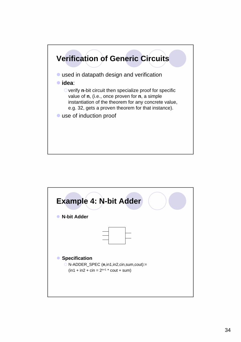
Verification of Generic Circuits

used in datapath design and verificationidea:

verify n-bit circuit then specialize proof for specific value of n, (i.e., once proven for n, a simple instantiation of the theorem for any concrete value, e.g. 32, gets a proven theorem for that instance).

use of induction proof

Example 4: N-bit Adder

N-bit Adder

SpecificationN-ADDER_SPEC (n,in1,in2,cin,sum,cout):= (in1 + in2 + cin = 2n+1 * cout + sum)

35

Example 4: N-bit Adder

Implementation

1-bitADDER sum[n-1]

coutin1[n-1]

in2[n-1]

cin

1-bitADDER

1-bitADDER

in1[n-2]

in2[n-2]

in1[0]

in2[0]

sum[n-2]

sum[0]

w

N-bit Adder (cont’d)

Implementationrecursive definition:N-ADDER_IMP(n,in1[0..n-1],in2[0..n-1],cin,sum[0..n-1],cout):=∃ w. N-ADDER_IMP(n-1,in1[0..n-2],in2[0..n-2],cin,sum[0..n-2],w) ∧

N-ADDER_IMP(1,in1[n-1],in2[n-1],w,sum[n-1],cout)Note:

N-ADDER_IMP(1,in1[i],in2[i],cin,sum[i],cout) = ADDER_IMP(in1[i],in2[i],cin,sum[i],cout)

Data abstraction function (vn: bitvec → nat) to relate bit vctors to natural numbers:

vn(x[0]):= bn(x[0])vn(x[0,n]):= 2n * bn(x[n]) + vn(x[0,n-1]

36


Proof goal:∀ n, in1, in2, cin, sum, cout.N-ADDER_IMP(n,in1[0..n-1],in2[0..n-1],cin,sum[0..n-1],cout)⇒ N-ADDER_SPEC(n, vn(in1[0..n-1]), vn(in2[0..n-1]), vn(cin),

vn(sum[0..n-1]), vn(cout))

can be instantiated with n = 32:∀ in1, in2, cin, sum, cout.N-ADDER_IMP(in1[0..31],in2[0..31],cin,sum[0..31],cout)⇒ N-ADDER_SPEC(vn(in1[0..31]), vn(in2[0..31]), vn(cin), vn(sum[0..31]), vn(cout))


Proof by induction over n:basis step:N-ADDER_IMP(0,in1[0],in2[0],cin,sum[0],cout)⇒ N-ADDER_SPEC(0,vn(in1[0]),vn(in2[0]),vn(cin),vn(sum[0]),vn(cout))

induction step:[N-ADDER_IMP(n,in1[0..n-1],in2[0..n-1],cin,sum[0..n-1],cout) ⇒N-ADDER_SPEC(n,vn(in1[0..n-1]),vn(in2[0..n-1]),vn(cin),vn(sum[0..n-1]),vn(cout))]⇒[N-ADDER_IMP(n+1,in1[0..n],in2[0..n],cin,sum[0..n],cout) ⇒N-ADDER_SPEC(n+1,vn(in1[0..n]),vn(in2[0..n]),vn(cin),vn(sum[0..n]),vn(cout))]

37


Notes:basis step is equivalent to 1-bit adder proof, i.e.ADDER_IMP(in1[0],in2[0],cin,sum[0],cout)⇒ ADDER_SPEC(bn(in1[0]),bn(in2[0]),bn(cin),bn(sum[0]),bn(cout))

induction step needs more creativity and work load!

Practical Issues of Theorem Proving

No fully automatic theorem provers. All require human guidance in indirect form, such as:

When to delete redundant hypotheses, when to keep a copy of a hypothesisWhy and how (order) to use lemmas, what lemma to use is an artHow and when to apply rules and rewritesInduction hints (also nested induction)

38

Practical Issues of Theorem Proving

Selection of proof strategy, orientation of equations, etc.Manipulation of quantifiers (forall, exists)Instantiation of specification to a certain time and instantiating time to an expressionProving lemmas about (modulus) arithmeticTrying to prove a false lemma may be long before abandoning

PVS

39

Prototype Verification System (PVS)

Provides an integrated environment for the development and analysis of formal specifications.Supports a wide range of activities involved in creating, analyzing, modifying, managing, and documenting theories and proofs.

Prototype Verification System (cont’)

The primary purpose of PVS is to provide formal support for conceptualization and debugging in the early stages of the lifecycle of the design of a hardware or software system.In these stages, both the requirements and designs are expressed in abstract terms that are not necessarily executable.

40

Prototype Verification System (cont’)

The primary emphasis in the PVS proof checker is on supporting the construction of readable proofs.In order to make proofs easier to develop, the PVS proof checker provides a collection of powerful proof commands to carry out propositional, equality, and arithmetic reasoning with the use of definitions and lemmas.

The PVS Language

The specification language of PVS is built on higher-order logic

Functions can take functions as arguments and return them as valuesQuantification can be applied to function variables

There is a rich set of built-in types and type-constructors, as well as a powerful notion of subtype.Specifications can be constructed using definitions or axioms, or a mixture of the two.

41

The PVS Language (cont’)

Specifications are logically organized into parameterized theories and datatypes.Theories are linked by import and export lists.Specifications for many foundational and standard theories are preloaded into PVS as prelude theories that are always available and do not need to be explicitly imported.

A Brief Tour of PVS

Creating the specificationParsingTypecheckingProvingStatusGenerating LATEX

42

A Simple Specification Example

sum: TheoryBEGIN

n: VAR natsum(n): RECURSIVE nat =(IF n = 0 THEN 0 ELSE n + sum(n-1) ENDIF)MEASURE (LAMBDA n : n)closed_form: THEOREM sum(n) = (n * (n + 1)) / 2

END sum

Creating the Specification

Create a file with a .pvs extensionUsing the M-x new-pvs-file command (M-x nf) to create a new PVS file, and typing sum when prompted. Then type in the sum specification.Since the file is included on the distribution tape in the Examples/tutorial subdirectory of the main PVS directory, it can be imported with the M-x import-pvs-file command (M-x imf). Use the M-x whereis-pvs command to find the path of the main PVS directory.Finally, any external means of introducing a file with extension .pvs into the current directory will make it available to the system. ex: using vi.

43

Parsing

Once the sum specification is displayed, it can be parsed with the M-x parse (M-x pa) command, which creates the internal abstract representation for the theory described by the specification.If the system finds an error during parsing, an error window will pop up with an error message, and the cursor will be placed in the vicinity of the error.

Typechecking

To typecheck the file by typing M-x typecheck(M-x tc, C-c t), which checks for semantic errors, such as undeclared names and ambiguous types.Typechecking may build new files or internal structures such as TCCs. (when sum has been typechecked, a message is displayed in the minibuffer indicating the two TCCs were generated)

44

Typechecking (cont’)

These TCCs represent proof obligations that must be discharged before the sum theory can be considered typechecked.TCCs can be viewed using the M-x show-tccscommand.


% Subtype TCC generated (line 7) for n-1

% unchecked

sum_TCC1: OBLIGATION (FORALL (n : nat) : NOT n=0 IMPLIES n-1 >= 0);

% Termination TCC generated (line 7) for sum

% unchecked

sum_TCC2: OBLIGATION (FORALL (n : nat) : NOT n=0 IMPLIES n-1 < n);

45


The first TCC is due to the fact that sum takes an argument of type nat, but the type of the argument in the recursive call to sum is integer, since nat is not closed under substraction.

Note that the TCC includes the condition NOT n=0, which holds in the branch of the IF-THEN-ELSE in which the expression n-1 occirs.

The second TCC is needed to ensure that the function sum is total. PVS does not directly support partial functions, although its powerful subtyping mechanism allows PVS to express many operations that are traditionally regarded as partial.

The measure function is used to show that recursive definitions are total by requiring the measure to decrease with each recursive call.

Proving

We are now ready to try to prove the main theoremPlace the cursor on the line containing the closed form theorem and type M-x prove M-x pr or C-c pA new buer will pop up the formula will be displayed and the cursor will appear at the Rule prompt indicating that the user can interact with the prover

46

Proving (cont’)

First, notice the display, which consists of a single formula labeled {1} under a dashed line.This is a sequent: formulas above the dashed lines are called antecedents and those below are called succedents

The interpretation of a sequent is that the conjunction of the antecedents implies the disjunction of the succedentsEither or both of the antecedents and succedents may be empty

Proving (cont’)

The basic objective of the proof is to generate a proof tree in which all of the leaves are trivially trueThe nodes of the proof tree are sequents and while in the prover you will always be looking at an unproved leaf of the treeThe current branch of a proof is the branch leading back to the root from the current sequentWhen a given branch is complete (i.e., ends in a true leaf), the prover automatically moves on to the next unproved branch, or, if there are no more unproven branches, notifies you that the proof is complete

47

Proving (cont’)

We will prove this formula by induction n.To do this, type (induct “n”)This generates two subgoals the one displayed is the base case where n is 0To see the inductive step type (postpone) which postpones the current subgoal and moves on to the next unproved one Type (postpone) a second time to cycle back to the original subgoal (labeled closed_form.1)

Proving (cont’)

To prove the base case, we need to expand the denition of sum, which is done by typing (expand “sum”)After expanding the denition of sum, we send the proof to the PVS decision procedures, which automatically decide certain fragments of arithmetic, by typing (assert)This completes the proof of this subgoal and the system moves on to the next subgoal which is the inductive step

48

Proving (cont’)

The first thing to do here is to eliminate the FORALL quantifierThis can most easily be done with the skolem! command, which provides new constants for the bound variablesTo invoke this command type (skolem!) at the promptThe resulting formula may be simplified by typing (flatten), which will break up the succedent into a new antecedent and succedent

Proving (cont’)

The obvious thing to do now is to expand the denition of sum in the succedent. This again is done with the expand command, but this time we want to control where it is expanded, as expanding it in the antecedent will not help. So we type (expand “sum” +), indicating that we want to expand sum in the succedent

49

Proving (cont’)

The final step is to send the proof to the PVS decision procedures by typing (assert)The proof is now complete the system may ask whether to save the new proof and whether to display a brief printout of the proof

closed_form :

| - - - - - - -{1} (FORALL (n : nat) : sum(n) = (n * (n + 1)) / 2)

Rule? (induct “n”)Inducting on n,this yields 2 subgoalsclosed_form.1 :

| - - - - - - -{1} sum(0) = (0 * (0 + 1)) / 2

Rule? (postpone)Postponing closed_form.1

50

closed_form.2 :

| - - - - - - -{1} (FORALL (j : nat) :

sum(j) = (j * (j + 1)) / 2IMPLIES sum(j + 1) = ((j + 1) * (j + 1 + 1)) / 2

Rule? (postpone)Postponing closed_form.2

closed_form.1 :

| - - - - - - -{1} sum(0) = (0 * (0 + 1)) / 2

Rule? (expand “sum”)(IF 0 = 0 THEN 0 ELSE 0 + sum(0 - 1) ENDIF)

simplifies to 0Expanding the definition of sum,this simplifies to:closed_form.1 :

| - - - - - - -{1} 0 = 0 / 2

Rule? (assert)Simplifying, rewriting, and recording with decision procedures,

This completes the proof of closed_form.1.

closed_form.2 :

| - - - - - - -{1} (FORALL (j : nat) :

sum(j) = (j * (j + 1)) / 2IMPLIES sum(j + 1) = ((j + 1) * (j + 1 + 1)) / 2

51

Rule? (skolem!)Skolemizing,this simplifies to:closed_form.2 | - - - - - - -{1} sum(j ! 1) = (j ! 1 * (j ! 1 + 1)) / 2

IMPLIES sum(j ! 1 + 1) = ((j ! 1 + 1) * (j ! 1 + 1 + 1)) / 2

Rule? (flatten)Applying disjunctive simplification to flatten sequent,This simplifies to:closed_form.2 :

{-1}sum(j ! 1) = (j ! 1 * (j ! 1 + 1)) / 2| - - - - - - -

{1} sum(j ! 1 + 1) = ((j ! 1 + 1) * (j ! 1 + 1 + 1)) / 2

Rule? (expand “sum” +)(IF j ! 1 + 1 = 0 THEN 0 ELSE j ! 1 + 1 + sum(j ! 1 + 1 - 1) ENDIF)simplifies to 1 + sum(j ! 1) + j ! 1Expanding the definition of sum,this simplifies to:closed_form.2:

[-1] sum(j ! 1) = (j ! 1 * (j ! 1 + 1)) / 2| - - - - - - -

{1} 1 + sum(j ! 1) + j ! 1 = (2 + j ! 1 + (j ! 1 * j ! 1 + 2 * j ! 1)) / 2

Rule? (assert)Simplifying, rewriting, and recording with decision procedures,

This completes the proof of closed_form.2.

Q.E.D

Run time = 5.62 secs.Real time= 58.95 secs.

52

Status

Type M-x status-proof-theory (M-x spt) and you will see a buffer which displays the formulas in sum (including the TCCs), along with an indication of their proof status

This command is useful to see which formulas and TCCs still require proofs

Another useful command is M-x status-proofchain (M-x spc), which analyzes a given proof to determine its dependencies

Generating LATEX

Type M-x latex-theory-view (M-x ltv). You will be prompted for the theory name ─ type sum, or just Return if sum is the defaultAfter a few moments the previewer will pop up displaying the sum theory, as shown below.

53

Generating LATEX (cont’)

sum: THEORYBEGINn: VAR natsum(n): RECURSIVE nat =

(IF n = 0 THEN 0 ELSE n + sum(n - 1) ENDIF)MEASURE (λ n : n)

closed_form: THEOREM sum(n) = (n * (n + 1)) / 2END sum

Generating LATEX (cont’)

Finally using the M-x latex-proof command, it is possible to generate a LATEX file from a proof

Expanding the definition of sum

closeed_form.2:'

0{ 1} ( ' ( ' 1)) / 2j

ii j j

=− = × +∑

' 1 1

0{1} (IF ' 1 0 THEN 0 ELSE ' 1 ENDIF) (( ' 1) ( ' 1 1)) / 2j

ij j i j j+ −

=+ = + + = + × + +∑

54

Conclusions

Advantages of Theorem ProvingHigh abstraction and expressive notationPowerful logic and reasoning, e.g., inductionCan exploit hierarchy and regularity, puts user in controlCan be customized with tactics (programs that build larger proofs steps from basic ones)Useful for specifying and verifying parameterized (generic) datapath-dominated designsUnrestricted applications (at least theoretically)

Conclusions

Limitations of Theorem Proving:Interactive (under user guidance): use many lemmas, large numbers of commandsLarge human investment to prove small theoremsUsable only by experts: difficult to prove large / hard theoremsRequires deep understanding of the both the design and HOL (while-box verification)must develop proficiency in proving by working on simple but similar problems.Automated for narrow classes of designs

Theorem proving -...

Documents

Transcript of Theorem proving -...