Theme V – Models and Techniques for

Analyzing Seismicity

Basic models of seismicity: Temporal models

Jiancang Zhuang1 • David Harte2 • Maximilian J. Werner3 •

Sebastian Hainzl4 • Shiyong Zhou5

1. Institute of Statistical Mathematics 2. Statistics Research Associates 3. Department of Geosciences, Princeton University 4. Institute of Geosciences, University of Potsdam 5. Department of Geophysics, Peking University

How to cite this article:

Zhuang, J., D. Harte, M.J. Werner, S. Hainzl, and S. Zhou (2012), Basic models of

seismicity: temporal models, Community Online Resource for Statistical Seismicity

Analysis, doi:10.5078/corssa-79905851. Available at http://www.corssa.org.

Document Information:

Issue date: 14 August 2012 Version: 1.0

2 www.corssa.org

Contents

1 Introduction . . . . . . . . . . . . . . . . . . . . . . . . . . . . . . . . . . . . . . . . . . . . . . . . . . . . . 3

2 Basic mathematical concepts . . . . . . . . . . . . . . . . . . . . . . . . . . . . . . . . . . . . . . . . . . . 4

3 Long-term temporal models . . . . . . . . . . . . . . . . . . . . . . . . . . . . . . . . . . . . . . . . . . . . 84 Temporal clustering models . . . . . . . . . . . . . . . . . . . . . . . . . . . . . . . . . . . . . . . . . . . . 19

5 Transformed time sequence and residual analysis . . . . . . . . . . . . . . . . . . . . . . . . . . . . . . . . 33

6 Related software . . . . . . . . . . . . . . . . . . . . . . . . . . . . . . . . . . . . . . . . . . . . . . . . . . 357 Summary . . . . . . . . . . . . . . . . . . . . . . . . . . . . . . . . . . . . . . . . . . . . . . . . . . . . . . 35

Basic models of seismicity: Temporal models 3

Abstract In this and subsequent articles, we present an overview of some mod-els of seismicity that have been developed to describe, analyze and forecast theprobabilities of earthquake occurrences. The models that we focus on are not onlyinstrumental in the understanding of seismicity patterns, but also important toolsfor time-independent and time-dependent seismic hazard analysis. We intend toprovide a general and probabilistic framework for the occurrence of earthquakes.In this article, we begin with a survey of simple, one-dimensional temporal modelssuch as the Poisson and renewal models. Despite their simplicity, they remain highlyrelevant to studies of the recurrence of large earthquakes on individual faults, to thedebate about the existence of seismic gaps, and also to probabilistic seismic hazardanalysis. We then continue with more general temporal occurrence models such asthe stress-release model, the Omori-Utsu formula, and the ETAS (Epidemic TypeAftershock Sequence) model.

1 Introduction

In this article, we present an overview of several temporal point-process models thatwere well studied during the 1990’s and 2000’s. We cannot go through all the ex-isting interesting models, and we only focus on some generic models, since most ofthe complicated models are constructed on the basis of these elegant generic mod-els. These models include the Poisson model, the renewal models, the Omori-Utsuformula, the ETAS (Epidemic Type Aftershock Sequence) model, and the stressrelease model. To address them systematically, we classify these models into thefollowing four classes: (1) 1D/temporal models, which include the stationary andnon-stationary Poisson model, the renewal model, the Omori-Utsu (Reseanberg-Jones) model, temporal ETAS models and single-region stress release models; (2)discrete multi-region models, including linked stress release models and self- andmutually exciting models; (3) spatiotemporal models, including homogeneous andnon-homogeneous Poisson models, space-time ETAS models; and, (4) models withauxiliary information, which incorporate information from observation or/and cal-culation results of other physical variables. In this article, we only discuss modelsfrom Class 1, i.e., temporal models that are formulated only based on the infor-mation of the catalogs. Please see other papers in this series for basic models fromthe 2nd and 3rd classes, and the CORSSA articles by Hainzl et al and Iwata (thistheme) for the 4th class of models.

To illustrate how to utilize these models for seismicity analysis, we give examplesthat are extracted from various published papers. We encourage the reader to repeatthese examples and to apply similar analysis to their own datasets.

4 www.corssa.org

2 Basic mathematical concepts

Earthquakes are caused by the rapid energy release accompanying the movementor fracture of faults in the crust or upper mantle of the earth, causing groundshaking of a duration from seconds to several minutes. However, generally only point-information is available for each earthquake, namely the origin time, hypocenter andmagnitude. If we compress the time axis of the seismograph to view all the recordsof earthquakes in a large time scale, the waveforms of each earthquake become apulse. We treat earthquakes as points in time and space. Such idealization enablesus to study the earthquake process by using point process models.

Mathematically, a point process is a random object that takes value of a countablesubset in a given spatiotemporal space. Here we can simply regard a point process asa type of stochastic model that defines probabilistic rules for the occurrence of points(i.e., earthquakes) in time and/or space. As well as purely temporal point processmodels, we consider in this article marked point processes that include earthquakemagnitudes. In a marked point process, a mark or size (e.g., magnitude) is assignedto each point.

Denote a point process in time by N and a certain temporal location by t. Weassume in the following discussions that we have known observations up to timet. The most important characteristic is the waiting time, say u, to the next eventfrom time t. We consider the following cumulative probability distribution functionof waiting time

Ft(u) = Prfrom t onwards, waiting time to next event ≤ u , (1)

with corresponding probability density function (p.d.f.)

ft(u) du = Prfrom t onward, waiting time is between u and u+ du , (2)

the survival function

St(u) = Prfrom t on, waiting time > u = Prno event occurs between t and t+ u, (3)

and the hazard function

ht(u) du = Prnext event occurs between t+ u and t+ u+ du

| it does not occur between t and t+ u.. (4)

Basic models of seismicity: Temporal models 5

One can easily prove that these functions are related in the following ways:

St(u) = 1− Ft(u) =

∫ ∞u

ft(s) ds = exp

[−∫ u

0

ht(s) ds

], (5)

ft(u) =dFtdu

= −dStdu

= ht(u) exp

[−∫ u

0

ht(s) ds

], (6)

ht(u) =ft(u)

St(u)= − d

du[logSt(u)] = − d

du[log(1− Ft(u))]. (7)

In the above equations, the first and second equality signs in each are obvious.Here we only outline how to derive the third equality signs in each. Equation (7)obtained from (4), i.e.,

ht(u) du =Prnext event occurs between t+ u and t+ u+ du

Prthe waiting time is greater than u.

=f(u) du

S(u)= −d logS(u).

To obtain the exponential term in (5), replace u by x in the above equality andintegrate both sides with respect to x from 0 to u to get∫ u

0

ht(x) dx = −∫ u

0

d logS(x) = log S(0)− logS(u) = − logS(u), (8)

i.e.,

S(u) = exp

[−∫ u

0

ht(x) dx

]. (9)

The last equality sign in (6) can be proved by taking the derivative of the aboveequation with respect to u.

In the above concepts, the hazard function ht is the key to understand our theorybecause it has the nice property of additivity. Suppose that a point process Nconsists of two independent sub-process, N1 and N2. Using the notation in (1) to(7) for N and denoting the waiting time distribution function, the survival function

and the hazard function of the sub-processes by F(i)t , S

(i)t and h

(i)t , respectively, with

i = 1 or 2, respectively, for N1 or N2. Then, we can prove

Ft(u) = F(1)t (u) + F

(2)t (u)− F (1)

t (u)F(2)t (u), (10)

ft(u) = f(1)t (u) + f

(2)t (u)− f (1)

t (u)F(2)t (u)− F (1)

t (u) f(2)t (u), (11)

ht(u) =ft(u)

1− Ft(u)=

f(1)t (u)

1− F (1)t (u)

+f

(2)t (u)

1− F (2)t (u)

= h(1)t (u) + h

(2)t (u). (12)

6 www.corssa.org

Another property of the hazard function is the following: if there is no eventoccurring between t and t + u and v ≥ u ≥ 0, then ht(v) = ht+u(v − u). This isfollowed by conditioning on no event occuring in (t, t+ u], then, when x ≥ 0.

St+u(x) = Prno event occurs in (t+ u, t+ u+ x) | no event occurs in (t, t+ u]

=Prno event occurs in either (t+ u, t+ u+ x) or (t, t+ u]

Prno event occurs in (t, t+ u]

=Prno event occurs in (t, t+ u+ x)

Prno event occurs in (t, t+ u]

=St(u+ x)

St(u)(13)

with x ≥ 0 and so

ht+u(x) =d

dxlogSt+u(x) =

d

dxlogSt(u+ x) = ht(u+ x). (14)

If we set x = 0 in the above equation, we have ht(u) = ht+u(0) when no events occurin (t, t + u], i.e., h collapses to a function of one variable. Thus, as a function of t,ht(0) is identical to ht0(t− t0) from a time t0, until the occurrence of another event,say t1, where ht(0) is identical to ht1(t− t1).

If an event occurs at t, then ht(0) has two possible explanations: one is the hazardfunction at t − tprev from the occurrence time tprev of the last previous event, theother is the hazard function at 0 from the event occurring at t. To distinguish them,we use ht−(0) and ht+(0) for the first and the second explanations, respectively.Conventionally, the first explanation is used for ht(0), i.e., ht(0) = ht−(0).

Example 1 If the distribution time from t is an exponential distribution, i.e.,

Ft(u) = 1− exp[−λu], and ft = λ exp[−λu], (15)

where λ is a positive constant, then

ht(u) = λ. (16)

This is the case of the Poisson process, which will be discussed in detail in nextsection.

Since the function ht(0) plays a key role in our understanding of the theory ofpoint processes, it is worthwhile to give it a specific name. Nowadays, it is usuallynamed as the conditional intensity and denoted by λ(t). Researchers also frequentlywrite it as λ(t|Ht), where Ht represents the observation history up to time t but notincluding t, since the value of λ(t) also can depend on what is in the observationhistory before t, but not on what happens at t.

Basic models of seismicity: Temporal models 7

From the definition of the hazard function, we have

λ(t) dt = Prone or more events occur in [t, t+ dt) | Ht. (17)

This is usually used as the definition of the conditional intensity. When the pointprocess N is simple, i.e., there is at most 1 event occurring at the same time location,then PrN [t, t + dt) > 1 = o(dt). Using this relationship, λ(t) can be also definedas follows:

E [N [t, t+ dt) | Ht] =∞∑n=0

nPrN [t, t+ dt) = n | Ht

≈ PrN [t, t+ dt) = 1 | Ht+ o(dt)

≈ λ(t) dt+ o(dt). (18)

The conditional intensity has a natural form for the purpose of forecasting.Given an observed dataset of a point process N , say t1, t2, · · · , tn, in a given

time interval [S, T ]. The likelihood function L is the joint probability density ofwaiting times to each of these events, i.e.,the joint probability that the waiting timefrom S is in the range (t1 − S, t1 − S + dt1) and the waiting time from t1 is in therange (t2−t1, t2−t1 +dt2) and so on, with the final term being that the waiting timefrom tn is greater than (T − tn). The probability each of these terms is conditionalon what has happened previously, so we can write the likelihood function as

L(N ;S, T ) dt1 dt2 · · · dtn

= PrThe waiting time from S is in (t1 − S, t1 − S + dt1)×PrThe waiting time from t1 is in (t2 − t1, t2 − t1 + dt2) | what happens before t1× · · ·×PrThe waiting time from tn is greater than T − tn | what happens before tn

= fS(t1) dt1 × ft1(t2 − t1) dt2 × · · · × ftn−1(tn − tn−1) dtn × Stn(T − tn)

= hS(t1 − S) exp

[−∫ t1

S

hS(u− S) du

]dt1

×n−1∏i=1

hti(ti+1 − ti) exp

[−∫ ti+1

ti

hti(u− ti) du

]dti

exp

[−∫ T

tn

htn(u− tn) du

](∵ (6))

=

[n∏i=1

hti(0) dti

]exp

[−∫ T

S

hu(0) du

]=

[n∏i=1

λ(ti) dti

]exp

[−∫ T

S

λ(u) du

]. (19)

We usually write the above formula as its logarithm, i.e.,

logL(N ;S, T ) =n∑i=1

log λ(ti)−∫ T

S

λ(u) du. (20)

8 www.corssa.org

A direct use of the likelihood function is for parameter estimation: when the modelinvolves some unknown regular parameters, say θ, we can estimate θ through max-imizing the likelihood, i.e., the MLE (maximum likelihood estimate) is

θ = argθ maxL(N ;S, T ; θ). (21)

Given several models fit to the same dataset, the optimal one can be selected byusing the Akaike Information Criterion (AIC, see Akaike 1974). The statistic

AIC = −2 maxθ

logL(θ) + 2kp (22)

is computed for each of the models fit to the data, where kp is the total number ofestimated parameters for a given model. Comparing models with different numbersof parameters, the addition of the quantity 2kp roughly compensates for the addi-tional flexibility that the extra parameters provide. The model with the lowest AICvalue is selected as the optimal choice for forward prediction purposes.

3 Long-term temporal models

In this section, we present the one-dimensional temporal models for long-term earth-quake forecasting, including Poisson models, renewal models and stress release mod-els. Roughly speaking, these models are intended to be used at time scales of 10 to100 years or even longer.

3.1 Stationary Poisson models

We suppose that the readers of this section already have some related backgroundknowledge of the Poisson process; if not, the readers are referred to Introduction toProbability Models (Ross 2003).

The Poisson process is named after the French mathematician Simeon-DenisPoisson (1871-1840). The process is also known as the model of complete random-ness. Thus, it naturally serves as the null model in many hypothesis tests to clarifywhether systematic structure is contained in the observations. For example, Gard-ner and Knopoff (1974) discussed whether the seismicity in California is Poissonianor not after the aftershock clusters are removed. Furthermore, the stationary Pois-son process forms the basis of most of today’s probabilistic seismic hazard analysis(Cornell 1968).

Let N(a, b) be the number of events in a point process N that fall in the timeinterval (a, b). A point process is called a stationary Poisson process if the systemhas the following characteristics:

Basic models of seismicity: Temporal models 9

a) Independent increments: The numbers of events occurring in two disjoint timeintervals are independent of each other. That is,

PrN(a, b) = m,N(c, d) = n = PrN(a, b) = mPrN(c, d) = n (23)

for all non-negative integers m, n, and any interval pairs (a, b) ∩ (c, d) = ∅.b) Stationarity: The probability distribution of the number of events falling in a

time interval only depends on the length of the time interval.c) Simplicity: There is never an occasion that two or more events occur simultane-

ously.

It can be shown that a stationary Poisson process has the following properties:

a) The number of events occurring in an interval of length S has a Poisson distri-bution, i.e.,

PrN(a, a+ S) = n =λnSn

n!e−λS, (24)

where λ is the long term average of the number of events in an interval of unitlength.

b) Given a fixed time, the forward occurrence time tf (time to next event) and thebackward occurrence time tb (time back to the previous event) have the sameexponential distribution as the waiting time τ between two consecutive events,i.e.,

Prtf < x = Prtb < x = Prτ < x = 1− e−λx. (25)

c) The mean and the variance of the number of observations are the same:

E [N(a, b)] = λ(b− a), Var [N(a, b)] = λ(b− a).

d) Binomial distribution. Given that n is the total number of events occurringin the interval [0, T ], then the number of events in [0, S], where S < T , is anon-negative integer-valued random variable from a binomial distribution withparameters (n, S/T ), i.e.,

PrN [0, S] = k | N [0, T ] = n =

(nk

)(S

T

)k (1− S

T

)n−k(26)

e) Uniform distribution: Given that at least one event occurs in [0, T ], then thelocation of an arbitrary event is uniformly distributed in [0, T ].

f) Beta distribution: Given that there are a total of n events occurring in [0, 1],n ≥ 1, the location t(k) of the kth event (k < n), from the left to the right, has abeta distribution, i.e.,

Prt(k) ∈ (x, x+ dx) | N [0, 1] = n =dx

B(k, n− k)xk−1(1− x)n−k−1, (27)

where B(x, y) =∫ 1

0tx−1(1− t)y−1 dt is the beta function.

10 www.corssa.org

Conditional intensity Recall the definition of the conditional intensity function of apoint process, which is defined by

λ(t)dt = Pr N [t, t+ dt) = 1 | Ht . (28)

For the stationary Poisson processes with rate λ, the right-hand side is λ dt exp[−dt]+o(dt), i.e., λ(t) = λ. This is why we use λ to denote both the rate of the Poissonprocess and the conditional intensity in the case of more general point processes.

Likelihood functions and maximum likelihood estimates of the Poisson process Sup-pose that all observations of a realization of a Poisson process with a rate of λ ona time interval [S, T ] is t1, t2, · · · , tn, where S ≤ t1 < t2 < · · · < tn < T . Thelikelihood of the observation is

L[S, T ;λ] = λne−λ(T−S), (29)

and the logarithm of the likelihood function is

logL(S, T ;λ) = n log λ− λ(T − S). (30)

Usually, the rate λ is unknown. We can estimate it through maximizing the likeli-hood function, i.e., the maximum likelihood estimate (MLE) of λ is

λ = argλ maxL(S, T ;λ) (31)

Taking the derivative of (30) and setting it to zero to obtain a maximum, we have

∂

∂λlogL(S, T ;λ)

∣∣∣∣λ=λ

= 0, (32)

which yieldsλ = n/(T − S), (33)

which is simply the average rate of events in the interval [S, T ].

3.2 Non-stationary Poisson models

A point process is a non-stationary Poisson process if it satisfies the independentincrements and simplicity conditions, but violates the stationarity condition. Con-sequently, the Poisson process has a rate that is a function of time, denoted byλ(t).

With the definition Λ(t) =∫ t

0λ(x) dx and Λ(t+s) =

∫ t+s0

λ(x) dx, the probabilityof observing n events in the interval [t, t+ s) is

PrN [t, t+ s) = n =e−(Λ(t+s)−Λ(t))[Λ(t+ s)− Λ(t)]n

n!.

Basic models of seismicity: Temporal models 11

That is, N [t, t+ s) is Poisson distributed with expectation value∫ t+st

λ(u) du whereλ(t) is the time dependent intensity. Also, given an event that falls in [S, T ], the prob-

ability density of its location is proportional to λ(·) on [S, T ], i.e., λ(t)/∫ TSλ(u) du.

Likelihoods and maximum likelihood estimates of non-stationary Poisson processesSuppose that the observation of a realization of a non-stationary Poisson processwith a rate of λ(t) on a time interval [S, T ] is t1, t2, · · · , tn, where S ≤ t1 < t2 <· · · < tn < T . In a similar way as for the stationary Poisson model, the likelihoodof the observations is

L(S, T ;λ) = e−∫ TS λ(u) du

∏i

λ(ti). (34)

The corresponding logarithm of the likelihood function is

logL(S, T ;λ) =∑i

log λ(ti)−∫ T

S

λ(u) du. (35)

There are relative few applications of non-stationary Poisson models in seismol-ogy. This type of model is usually used as a natural alternative to the null stationaryPoisson model when an apparent trend or seasonality is visible in the data. Some ex-amples of non-stationary Poisson models are the exponential trend model in Zhengand Vere-Jones (1994) and the polynomial trend models and the seasonality modelsin Ogata and Katsura (2004) and Ma and Vere-Jones (1997).

3.3 Renewal/recurrence models

Renewal models are simple extensions of the Poisson model. One of their uses isto model the characteristic recurrence of earthquakes on a particular fault or ina particular region. This class of models is widely used in seismicity and seismichazard analysis. For example, Field (2007) summarized how the Working Group onCalifornia Earthquake Probabilities (WGCEP) estimates the recurrence probabili-ties of large earthquakes on major fault segments using various recurrence modelsto produce the official California seismic hazard map. These models are sometimesjustified by the elastic rebound theory proposed by Reid (1910). According to histheory, large earthquakes release the elastic strain that has built up since the lastlarge earthquake. Some seismologists deduce that the longer it has been since thelast earthquake, the more probable is an imminent event (e.g. Nishenko and Buland1987; Nishenko 1991; Sykes and Menke 2006), while others contend that the datacontradict this view (e.g. Davis et al. 1989; Kagan and Jackson 1995). Renewalmodels are often used to quantitatively demonstrate whether earthquakes occurtemporally in clusters or quasi-periodically.

12 www.corssa.org

A renewal process is a generalization of the Poisson process. In essence, thePoisson process has independent identically distributed waiting times that are ex-ponentially distributed before the occurrence of the next event. A renewal processis defined as a point process with the waiting times having a more general distri-bution, which is not necessarily exponential distribution. In this section, we denotethe density function of the waiting times by f(·), which is also usually called therenewal density.

The conditional intensity of the renewal process can be derived as follows. Recallthat the time interval between any two adjacent events is independent from otherintervals. This means that the occurrence of the next event depends only on the timeof the last event but not on the full history. Thus, from Section 1, the conditionalintensity function is the same as the hazard function, i.e.,

λ(t) =f(t− tN(t−))

1− F (t− tN(t−)), (36)

where tN(t−) is the occurrence time of the last event before t and F is the cumulativeprobability function of f .

The following probability functions are often chosen as the the renewal densities.

1. The gamma density

f(u; k, θ) = uk−1 e−u/θ

θk Γ (k), for u ≥ 0 and k, θ > 0 , (37)

with a hazard function

h(u; k, θ) =uk−1 e−

uθ

θkΓuθ(k, u

θ), (38)

where θ is called the scale parameter, k the shape parameter, and Γ and Γαare the gamma and the incomplete gamma functions, respectively, defined byΓ (x) =

∫∞0tx−1e−t dt and Γα(x) =

∫∞αtx−1e−t dt.

2. The log-normal density function is

f(u;µ, σ) =1

uσ√

2πe−

(ln(u)−µ)2

2σ2 , for u ≥ 0, (39)

with a hazard function

h(u;µ, σ) =2

uσ√

2π

e−(ln(u)−µ)2

2σ2

1− erf[

ln(u)−µσ√

2

] , (40)

Basic models of seismicity: Temporal models 13

where µ and σ are the mean and standard deviation of the variable’s naturallogarithm1. and erf is the error function.

3. The Weibull distribution is one of the most widely used lifetime distributionsin reliability engineering. It is named after Waloddi Weibull who described itin detail in 1951 (Weibull 1951). The probability density function of a Weibullrandom variable X is

f(u;µ, k) =

kµ

(uµ

)k−1

e−(u/µ)k u ≥ 0,

0 u < 0,(41)

where k > 0 is the shape parameter and µ > 0 is the scale parameter of the dis-tribution. Its cumulative distribution function is a stretched exponential function

F (u;µ, k) = 1− e−(u/µ)k

and its hazard function is

h(u; k, µ, k) =k

µ

(u

µ

)k−1

.

4. Kagan and Knopoff (1987) used the inverse Gaussian distribution to model theevolution of stress as a random walk with a tectonic drift. Later on, a partic-ularly interesting renewal model, called the Brownian passage-time model, wasintroduced by Matthews et al. (2002) and Ellsworth et al. (1999) based on theproperties of the Brownian relaxation oscillator (BRO). In this conceptual modelof Matthews et al. (2002), the loading of the system has two components: (1) aconstant-rate loading component, λt, and (2) a random component, ε(t) = σW (t),that is defined as a Brownian motion (where W is a standard Brownian motionand σ is a nonnegative scale parameter). The Brownian perturbation process forthe state variable X(t) (see Figure 2 in Matthews et al. (2002)) is defined as:

X(t) = λt+ σW (t).

An event will occur when X(t) ≥ Xf ; event times are seen as “first passage”or “hitting” times of Brownian motion with drift. The BRO are a family ofstochastic renewal processes defined by four parameters: the drift or mean loading(λ), the perturbation rate (σ2), the ground state (X0), and the failure state(Xf ). On the other hand, the recurrence properties of the BRO (response times)are described by a Brownian passage-time distribution which is characterizedby two parameters: (1) the mean time or period between events, (µ), and (2)

1 If X is a normal random variable with mean µ and variance σ2, then Y = expX has a log-normal distribution

with a density of (39).

14 www.corssa.org

the aperiodicity of the mean time, α, which is equivalent to the coefficient ofvariation (defined in as the ratio of the variance to the mean occurrence time).The probability density for the Brownian passage-time (BPT) model is given by:

f(t;µ, α) =( µ

2πα2t3

) 12

exp

−(t− µ)2

2α2µt

, t ≥ 0 (42)

with a cumulative probability function

F (t;µ, α) = Φ

(t− µα√µx

)+ exp

(2

α2

)Φ

(− t+ µ

α√µx

), (43)

where Φ is the cumulative probability distribution function of a standard normalrandom variable, i.e., F is the inverse Gaussian or Wald distribution.

Forward recurrence time In practice, we usually do not start our observation at theoccurrence of an event. Then we are interested in the distribution of waiting timesuntil the next event starting from this starting time, i.e., the forward recurrencetime from an arbitrary time. This problem is equivalent to finding the distributionof the distance between an arbitrary point to the next event in the time line, andcan be solved in three steps.

1. Assume that the length of each inter-event interval ∆ has a density f with finitemean µ0, i.e.,

∫∞0u f(u) du = µ0.

2. The arbitrary time point falls in each inter-event interval ∆ with a probabilityproportional to its length. That is to say, this arbitrary time is uniformly dis-tributed on the time axis and has more chances to fall in larger intervals; or,PrArbitrary point falls in ∆ | ∆ ∈ [z, z + dz] ∝ z.

3. From 2, given the length ∆ = z of the inter-event interval that the arbitrary timefalls in, the probability that the forward recurrence time X is less than t is 1 ifz < t, or t/z if z ≥ t. In other words, the probability that the forward recurrencetime X is greater than t is 0 if z < t, or (z − t)/z if z ≥ t. In summary,

PrX ≥ t =

∫ ∞t

[PrArbitrary point falls in ∆ | ∆ ∈ [z, z + dz]

× Pr∆ ∈ [z, z + dz] × PrX > t | ∆ ∈ [z, z + dz)]

∝∫ ∞t

z f(z)(z − t)z

dz

=

∫ ∞t

(z − t)f(z) dz

= µc(t)− t[1− F (t)] (44)

Basic models of seismicity: Temporal models 15

where

µc(t) =

∫ ∞t

z f(z) dz.

Similarly, it can be shown that

PrX < t ∝ t[1− F (t)] + µ(t) (45)

where

µ(t) =

∫ t

0

z f(z) dz.

We find the normalizing factor in (44) by using

1 = PrX <∞ = PrX ≥ 0, (46)

which gives

PrX < t =t[1− F (t)]

µ0

+µ(t)

µ0

(47)

and

PrX ≥ t =µc(t)

µ0

− t [1− F (t)]

µ0

, (48)

where µ0 = E∆ =∫∞

0z f(z) dz.

It is easy to see that the phrase “the forward recurrence time” can be replacedby “the backward recurrence time” in the above discussion. That is to say, thebackward recurrence time Y has the same distribution as the forward distributionfunction. The density function wf of the forward recurrence times is obtained bytaking the derivative of (47), i.e.,

wf (t) =1− F (t)

µ0

, (49)

with corresponding hazard function

hf (t) =wf (t)

PrX > t=

1− F (t)

µc(t)− t[1− F (t)]. (50)

16 www.corssa.org

Table 1 Historical Earthquakes at Nankai Trough (DATA FILE: example2.data)

Occurrence times Years

t1 684

t2 887

t3 1099t4 1233

t5 1361t6 1498

t7 1605

t8 1707t9 1854

t10 1946

Table 2 Results from fitting renewal models to the Nankai Trough data

Model MLE logL AIC

Poisson λ = 7.092× 10−3 -59.488 120.975

Gamma k = 7.768, θ = 16.865 -54.156 112.312log-normal µ = 4.813, σ = 0.365 -54.580 113.160

Weibull k = 2.886, µ = 144.849 -55.176 114.351BPT µ = 123.881, α = 0.419 -55.978 113.954

Likelihood function Suppose that the realization of a renewal process is t1, t2, · · · , tnin [0, T ], and we do not know what happens before time 0. The likelihood functioncan be written as

L(0, T ; ·) = wf (t1)×n∏i=2

f(ti − ti−1)× F (T − tn). (51)

Another form of the likelihood is through the conditional intensity function,

logL(0, T ; ·) =∑

i: ti∈[0,T ]

log λ(ti)−∫ T

0

λ(u) du. (52)

It can be shown that both forms are equivalent.

Example 2 Table 1 [Data file: example2.data] lists 10 great earthquakes of M8+that have occurred in the Nankai Trough south of Japan since 600 A.D., taken fromTable 10.5 in Utsu (1999). Ogata (2002) analyzed this data set by using recurrencemodels and Bayesian methods to evaluate the uncertainties in the estimated occur-rence times. Here, as a simple illustration, we fit the Poisson and the four renewalmodels discussed in this section. The estimated parameters and the correspond-ing likelihood and AIC scores are listed in Table 2, indicating that, in this simpleexample, the Gamma model fits the data the best.

Basic models of seismicity: Temporal models 17

Among the models mentioned in this section, the BPT model has become themost popular one and has been used in obtaining some interesting results (see, e.g.,Ogata 2002 and Nomura et al. 2011). However, there is no clear evidence showingthat one model is superior to the others. This might be caused by the relativelylarge standard errors of the parameter estimates that are due to very few datapoints in the historical catalogs. Another reason may due to the nature of renewalprocesses (e.g., MacFadden and Weissblum 1965; Daley and Vere-Jones 2003, Pages77–79): The superposition of independent nontrivial renewal processes does notresult in a renewal process unless all of the superposed processes are simply Poisson.This property requires that the renewal process is applied to a fault system thatis relatively disjoint in behavior from the surrounding environment, or is loaded bya constant tectonic stressing rate. However, the identification of such fault systemsseems technically difficult in practice.

3.4 Stress release models

Based on the elastic rebound theory (Reid 1910), the stress release model was intro-duced in a series of papers by Vere-Jones and others (see, e.g., Zheng and Vere-Jones1991, 1994). It was extended to the linked stress release model by Shi et al. (1998),Liu et al. (1998), Lu et al. (1999), Lu and Vere-Jones (2000), and Bebbington andHarte (2001, 2003). This model assumes that the stress level in a certain regionis gradually built up, linearly with time by tectonic movements, and drops downsuddenly coinciding with earthquakes, i.e., the stress level at t, X(t), can be writtenas

X(t) = X(0) + ρt− S(t), (53)

where X(0) is the initial stress level, ρ is the constant loading rate from the tectonicmovements, and S(t) is the accumulated stress release from earthquakes in theperiod [0, t), namely

S(t) =∑i: ti<t

si . (54)

It is assumed that the stress release related to individual earthquakes scales withthe magnitude mi according to

si = 100.75mi , (55)

which is hinted from the Benioff strain. The conditional intensity is a monotonicallyincreasing function of the stress level, usually chosen as

λ(t) = Ψ(X) = eγX = exp[γ(X(0) + ρt− S(t))] = exp[a+ bt− c S(t)], (56)

18 www.corssa.org

where γ is a single parameter representing the strength and heterogeneity of theregional crust, and a = γ X(0), b = ργ, and c = γ are the final model parame-ters. The assumption of an exponential distribution is in agreement with laboratoryexperiments of stress corrosion where the mean waiting time until fracture can beapproximated by an exponential function of negative applied stress (Scholz 2002).

The amount of stress si released by an earthquake has a distribution with adensity function of ξ(s) and cumulative probability function Ξ(s), which is, forsimplification, assumed to be independent from the stress level. That is to say, thefull model has a conditional intensity function in the form of

λ(t, s) = Ψ [X(t)] ξ(s). (57)

Given the observations (ti, si) : i = 1, 2, · · · , n in a time period [T1, T2], the log-likelihood function for the full model is

logL(T1, T2; ·) =n∑i=1

log λi(ti, si)−∫ T2

T1

∫ ∞0

λ(u, v) dv du

=n∑i=1

log Ψ(X(ti))−∫ T2

T1

Ψ(X(u)) du+n∑i=1

log ξ(si). (58)

In the above equation, the first two terms are from the usual likelihood for puretemporal processes, and the third term represents the joint distribution of stressreductions caused by the earthquakes.

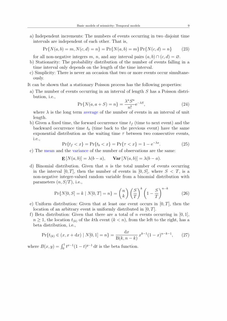
Usually, we consider the following three types of distributions for S: the Pareto,the truncated Pareto and the tapered Pareto distributions:

1. The Pareto distribution of S corresponds to the case where the magnitude dis-tribution follows the Gutenberg-Richter magnitude-frequency relation, i.e., theexponential distribution. It has a probability density function

ξ(s) =k − 1

S0

(s

S0

)−k; s ≥ S0, k > 1, (59)

where k is linked with the Gutenberg-Richter b-value by k = 43b+ 1.

2. The truncated Pareto distribution of s corresponds to the case where the magni-tude distribution follows the truncated Gutenberg-Richter magnitude-frequencyrelation. It has a probability density function

ξ(s) =k − 1

S0

[1−

(SuS0

)1−k] ( s

S0

)−k, S0 ≤ s ≤ Su, (60)

where Su and S0 are the upper and lower thresholds, respectively.

Basic models of seismicity: Temporal models 19

3. The tapered Pareto (or Kagan) distribution (see, Vere-Jones et al. 2001; Kaganand Schoenberg 2001) has a cumulative distribution function

Ξ(s) = 1−( sS 0

)−k+1

exp

(S0 − sSc

), S0 ≤ s <∞, (61)

and a density

ξ(s) =

(k−1

s+

1

Sc

)(s

S0

)−k+1

exp

(S0 − sSc

), S0 ≤ s <∞, (62)

where Sc is a parameter governing the strength of the exponential taper affectingfrequency of large events.

All three distributions are illustrated in Fig. 1.

The magnitude-frequency distribution of earthquake is well described by theGutenberg-Richter magnitude-frequency relation (Gutenberg and Richter 1944),which takes the form of an exponential distribution, i.e.,

Prmagnitude > m = 10−b(m−mc), m ≥ mc, (63)

where b is the so-called Gutenberg-Richter b-value. To reduce the possibility ofextremely large earthquakes in simulation, the following truncated form is alsooften adopted:

Prmagnitude > m =

10−b(m−mc) = e−β(m−mc), if mc ≤ m ≤Mmax,

0 otherwise,

where Mmax is the upper bound of magnitudes.

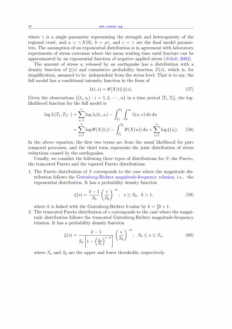
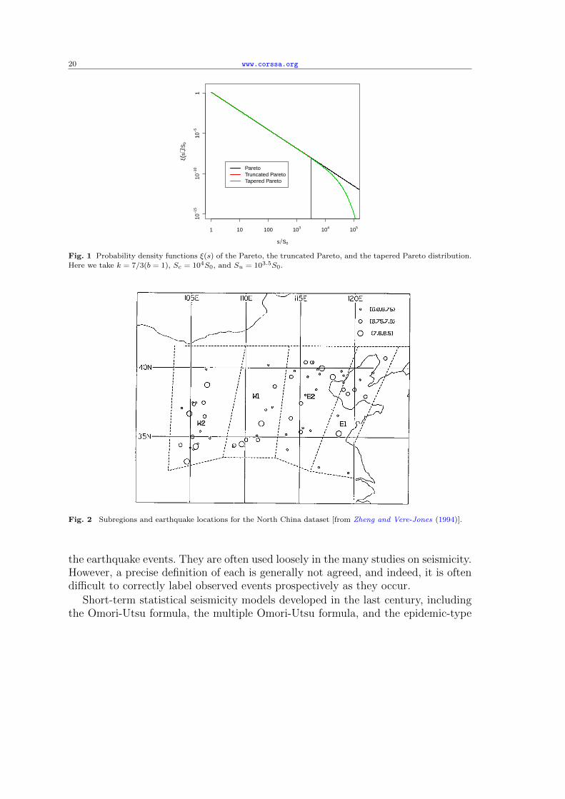
Example 3 The following example is taken from Zheng and Vere-Jones (1994) wherethe stress release model was fit to the historical catalog from North China duringthe period from 1480 to 1992. Table 3 (Data file example3.data) lists this historicalcatalog from North China, Figure 2 shows the division of subregions, and Table4 gives the corresponding results. Figure 3 shows the temporal variations of theconditional intensity functions in each subregion.

4 Temporal clustering models

On short time scales, seismicity has been shown to be clustered. The terms foreshock,main shock, aftershock, and earthquake swarm are concepts related the clustering of

20 www.corssa.org

s S0

ξ(s)

S0

10−1

510

−10

10−5

1

1 10 100 103 104 105

ParetoTruncated ParetoTapered Pareto

Fig. 1 Probability density functions ξ(s) of the Pareto, the truncated Pareto, and the tapered Pareto distribution.

Here we take k = 7/3(b = 1), Sc = 104S0, and Su = 103.5S0.

Fig. 2 Subregions and earthquake locations for the North China dataset [from Zheng and Vere-Jones (1994)].

the earthquake events. They are often used loosely in the many studies on seismicity.However, a precise definition of each is generally not agreed, and indeed, it is oftendifficult to correctly label observed events prospectively as they occur.

Short-term statistical seismicity models developed in the last century, includingthe Omori-Utsu formula, the multiple Omori-Utsu formula, and the epidemic-type

Basic models of seismicity: Temporal models 21

Table 3 DATA FILE: example3.data Historical large earthquake from north China, 1480-1996, reprinted fromZheng and Vere-Jones (1994).

Date Lat. Long. Mag. Reg. Date Lat. Long. Mag. Reg.

1484.01.29 40.40 116.10 6.70 W1 1487.08.10 34.30 108.90 6.20 E2

1501.01.19 34.80 110.10 7.00 E2 1502.10.17 35.70 115.30 6.50 W11536.10.22 39.60 116.80 6.00 W1 1548.09.13 38.00 121.00 7.00 W2

1556.01.23 34.50 109.70 8.00 E2 1561.07.25 37.50 106.20 7.20 E1

1568.04.25 34.40 109.00 6.70 E2 1568.05.15 39.00 119.00 6.00 W21573.01.10 34.40 104.10 6.70 E1 1587.04.10 35.20 113.80 6.00 W1

1597.10.06 38.50 120.00 7.00 W2 1604.10.25 34.20 105.00 6.00 E11614.10.23 37.20 112.50 6.50 E2 1618.05.20 37.00 111.90 6.50 E2

1618.11.16 39.80 114.50 6.50 W1 1622.03.18 35.50 116.00 6.00 W1

1622.10.25 36.50 106.30 7.00 E1 1624.02.10 32.40 119.50 6.00 W21624.04.17 39.80 118.80 6.20 W1 1624.07.04 35.40 105.90 6.00 E1

1626.06.28 39.40 114.20 7.00 W1 1627.02.15 37.50 105.50 6.00 E1

1634.01.- 34.10 105.30 6.00 E1 1642.06.30 35.10 111.10 6.00 E21654.07.21 34.30 105.50 8.00 E1 1658.02.03 39.40 115.70 6.00 W1

1665.04.16 39.90 116.60 6.50 W1 1668.07.25 35.30 118.60 8.60 W2

1679.09.02 40.00 117.00 8.00 W1 1683.11.22 38.70 112.70 7.00 E21695.05.18 36.00 111.50 8.00 E2 1704.09.28 34.90 106.80 6.00 E1

1709.10.14 37.40 105.30 7.50 E1 1718.06.29 35.00 105.20 7.50 E1

1720.07.12 40.40 115.50 6.70 W1 1730.09.30 40.00 116.20 6.50 W11739.01.03 38.80 106.50 8.00 E1 1815.10.23 34.80 111.20 6.70 E2

1820.08.03 34.10 113.90 6.00 W1 1829.11.19 36.60 118.50 6.00 W21830.06.12 36.40 114.20 7.50 W1 1831.09.28 32.80 116.80 6.20 W2

1852.05.26 37.50 105.20 6.00 E1 1861.07.19 39.70 121.70 6.00 W2

1879.07.01 33.20 104.70 8.00 E1 1882.12.02 38.10 115.50 6.00 W11885.01.14 34.50 105.70 6.00 E1 1888.06.13 38.50 119.00 7.50 W2

1888.11.02 37.10 104.20 6.20 E1 1920.12.06 36.70 104.90 8.50 E1

1922.09.29 39.20 120.50 6.50 W2 1937.08.01 35.40 115.10 7.00 W11945.09.23 39.50 119.00 6.20 W1 1966.03.22 37.50 115.10 7.20 W1

1967.03.27 38.50 116.50 6.30 W1 1969.07.18 38.20 119.40 7.40 W2

1975.02.04 40.70 122.80 7.30 W2 1976.04.06 40.20 111.10 6.20 E21976.07.28 39.40 118.00 7.80 W1 1976.09.23 39.90 106.40 6.20 E1

1979.08.25 41.20 108.10 6.00 E1 1989.10.18 40.00 113.70 6.00 E2

Table 4 Results from fitting the stress release model to the historical earthquakes from each of the four subregions

in North China. N represents the number of events in each subregion.

a b c logL (SRM) logL (Poisson) ∆AIC N

E1 -5.397 0.0209 0.571 -52.04 -56.76 -5.44 11E2 -3.900 0.0176 0.880 -83.34 -87.58 -4.48 22

W1 -2.764 0.0035 1.731 -50.36 -52.99 -1.24 11

W2 -5.152 0.0238 0.410 -91.97 -77.84 -7.75 18

aftershock sequence (ETAS) model, all emphasize the evolutionary nature of a de-veloping earthquake cluster. In this section, we give an introduction to these models.The models described in this section do not have a spatial component. Hence, thereis an implicit assumption that the spatial area is sufficiently small so that any given

22 www.corssa.org

Fig. 3 Conditional intensity curves for the four subregions of the North China dataset [from Zheng and Vere-Jones(1994)].

event can conceivably interact with all following events, regardless of their spatiallocations.

4.1 The Omori-Utsu formula

The Omori-Utsu formula describes the decay of the aftershock frequency with timeafter a mainshock as an inverse power law. When Omori (1894) was studying theaftershocks of the 1891 Ms8.0 Nobi earthquake, he first tried to use an exponentialdecay function to fit the data, but unsatisfactory results were obtained. Then hefound that the number of aftershocks occurring each day can be well described bythe equation

n(t) = K(t+ c)−1, (64)

Basic models of seismicity: Temporal models 23

where t is the time from the occurrence of the mainshock, K and c are constants.Utsu (1957) postulated that the decay of the aftershock numbers could vary, and

showed thatn(t) = K(t+ c)−p (65)

yields better fitting results. Equation (65) is now called the modified Omori formulaor Omori-Utsu formula.

The Omori-Utsu formula has been used extensively to analyze, model and forecastaftershock activity. Utsu et al. (1995) reviewed the values of p for more than 200aftershock sequences and found that it ranges between 0.6 and 2.5 with a medianof 1.1. He found no clear relationship between estimates of p-values and mainshockmagnitudes.

In the context of statistical seismology, we usually make use of (65) in the formof a conditional intensity function, given by

λ(t) =K

(t+ c)p. (66)

When the magnitude distribution of the aftershocks is also considered, the condi-tional intensity for the full model is written as

λ(t,m) =K s(m)

(t+ c)p, (67)

where s(m) is the magnitude probability density function and usually takes the formof the Gutenberg-Richter magnitude-frequency relation. This model has been usedby Reasenberg and Jones for forecasting aftershock activity (see, e.g., Reasenbergand Jones 1989, 1994). Therefore, some researchers also call (67) the Reasenberg-Jones model.

Likelihood of the single and multiple Omori-Utsu formulas Suppose that the oc-currence time of the mainshock is 0. As discussed in Section 2, given observationsN = (ti,mi) : i = 1, 2, · · · , n in the the time interval [S, T ], T > S ≥ 0, thelog-likelihood function for the model of the Omori-Utsu formula can be written inthe form

logL(N ;S, T ) =∑

i: ti∈[S,T ]

log λ(ti,mi)−∫M

∫ T

S

λ(u,m) du dm

=∑

i: ti∈[S,T ]

log λ(ti)−∫ T

S

λ(u) du+∑

i: ti∈[S,T ]

log s(mi), (68)

where the first two terms on the righthand side represent the contribution to thelikelihood from the occurrence times and the third term represents the contribution

24 www.corssa.org

Fig. 4 A plot of magnitudes against indices of the aftershocks of the 2008 Wenchuan earthquake in China. The

red line indicates the estimation of the completeness magnitude.

from the magnitudes. The parameters in the Omori-Utsu formula can be estimatedfrom maximizing the temporal part of the likelihood (first two terms in the righthandside)

∑i: ti∈[S,T ]

log λ(ti)−∫ T

S

λ(u) du

= N logK − p∑

i: ti∈[S,T ]

log(ti + c)− K

p− 1

[(S + c)1−p − (T + c)1−p] . (69)

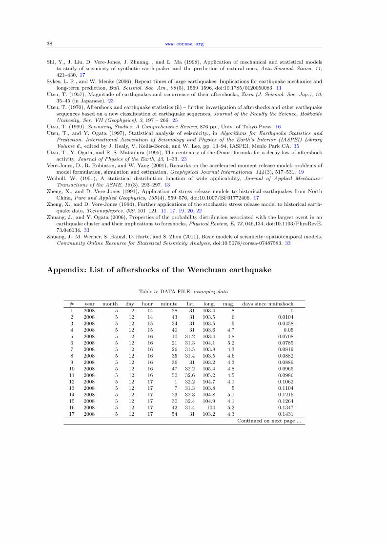
Example 4 The aftershock sequence of the 2008MS8.0 Wenchuan earthquake, China:Table 5 [Data file example4.data] lists the mainshock and the aftershocks (MS ≥ 4.0)of the Wenchuan earthquake (2009-5-12, Ms8.0), occurring within 25 days after themainshock. Since aftershocks immediately after a large mainshock are usually miss-ing due to detection and recording problems (see, e.g., Kagan and Jackson 1995),the Omori-Utsu formula should only be fit to a period where the records in theconsidered magnitude range are complete. A simple and direct way to detect thisstarting point is by plotting each event magnitude against its catalog sequentialnumber of event. As shown in Figure 4, we arbitrarily take T0 = 0.3 days, corre-sponding to the occurrence time of the 40th event. The estimated parameters fromfitting the Omori-Utsu formula are K = 45.228, c = 0.129 days, and p = 1.107; withlogL = 270.575.

Basic models of seismicity: Temporal models 25

Fig. 5 Comparison of the observed and modeled cumulative number of M ≥ 4-aftershocks of the Wenchuan

earthquake: observation (black) and Omori-Utsu formula (red).

Multiple Omori-Utsu formula It is often observed that not only mainshocks triggeraftershocks, but also large aftershocks may trigger their own aftershocks. To modelsuch phenomena, Utsu (1970) used the following model

λ(t) = K/(t− t0 + c)−p +

NT∑i=1

KiH(t− ti)(t− ti + ci)−pi

, (70)

where t0 is the occurrence time of the mainshock, ti, i = 1, . . . NT , define the oc-currence times of the triggering aftershocks and H is the Heaviside function. Thelikelihood for the multiple Omori-Utsu formula is sightly more complicated than forthe simple Omori-Ustu formula, but can be written in a similar way.

Example 5 This example is on the 1965 Rat Island earthquake of MW8.7 and itsaftershocks, and is taken from Ogata and Shimazaki (1984). Earthquakes within therange 170 − 180E and 48 − 55N and with magnitudes mb ≥ 4.7 are selected.An ordinary log-log plot of the daily number of events against time is time shownin Figure 6. The results from fitting a simple Omori-Utsu formula are

K = 85.088, c = 0.204, p = 1.055, AIC = −811.4,

and from the multiple formula, by assuming that the largest aftershock of MW7.6also has its own aftershocks, are

K = 82.284, K1 = 6.117, c = c1 = 0.204, p = p1 = 1.055, AIC = −873.4.

26 www.corssa.org

Fig. 6 An ordinary log-log plot of the number of aftershocks of the 1965 MW 8.7 Rat Island event per day against

time (Ogata and Shimazaki 1984). The curve represents the intensity function fitted to observed data points markedby the squares.

Here the AIC criteria selects the model where c = c1 and p = p1 as the best modelamong the class of models with NT = 1.

One difficulty in applying the multiple Omori-Utsu formula is to determine whichearthquakes are triggering events. The largest aftershocks often have secondary af-tershocks, but not always. We can use the techniques of residual analysis in Section5, as a diagnostic tool, to find out which events have secondary aftershocks.

4.2 The Epidemic-Type Aftershock Sequence (ETAS) model

In most cases, aftershock activity consists of secondary aftershock clustering as de-scribed by the multiple Omori-Utsu formula (70). However, even though possibletriggering events could potentially be determined through a residual analysis, sepa-rating triggering earthquakes from the others is difficult. Ogata (1988) generalizedthis model by not needing to make a distinction between triggering events and theother events. He proposed that each event, irrespective of whether it is a small ora big event, can in principle trigger its own offspring. More precisely, the temporal

Basic models of seismicity: Temporal models 27

conditional intensity of this model is

λ(t) = µ+∑i: ti<t

κ(mi) g(t− ti), (71)

or, the full form of the condition intensity for this marked point process is

λ(t,m) = s(m)

[µ+

∑i: ti<t

κ(mi) g(t− ti)

], (72)

where s(m) = β e−β(m−m0),m ≥ m0, is the p.d.f. form of the Gutenberg-Richterrelation, m0 being the magnitude threshold, κ(m) = A exp[α(m−m0)] is the meannumber of events directly triggered by an event of magnitude m and g(u) =(p − 1)(1 + t/c)−p/c is the probability density function (p.d.f.) of the time dif-ference between the parent event and its children, i.e., the p.d.f. form of the Omori-Utsu formula. Ogata (1988) named (71) the Epidemic-Type Aftershock Sequence(ETAS) model, based on an analogy with the spread of epidemics. The ETAS modelalso belongs to the more general class of self-exciting Hawkes processes (Hawkes1971a,1971b; Hawkes and Oakes 1974).

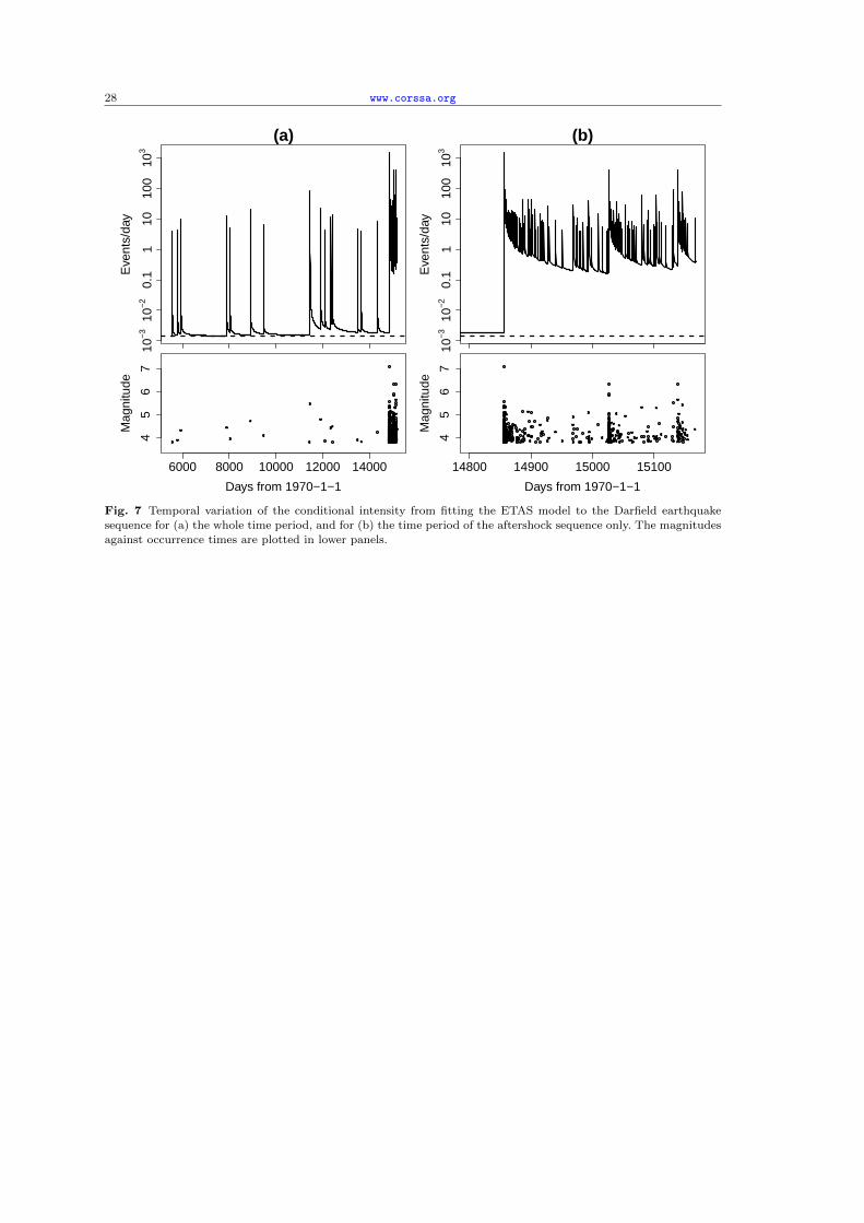
Example 6 [Data file: example6.data] The aftershock sequence of the Darfield earth-quake, New Zealand (MW7.1, 2010-9-4). The dataset is taken from the New Zealandcatalog compiled by GNS, in the region (43.2− 44.0S, 171.0− 173.5E) and in thetime interval from 1985-1-1 to 2011-7-13. The magnitude threshold is M3.8. By us-ing the ETAS fitting program in the SASeis software (Ogata 2006), the MLEs of themodel parameters are µ = 0.001414 (events/day), K = 10.32, c = 0.006006 (day),α = 1.832, p = 1.0167. Figure 7 shows the conditional intensity for the fitted ETASmodel.

Criticality and branching ratio A condition for stability of the ETAS model is thatthe process must be subcritical. In data analysis this important condition justifieswhether estimated model parameters are reasonable or irrational. Also, when ex-tending the ETAS model or specifying an explicit form of an ETAS-like branchingmodel, the stability conditions must be satisfied. Forecasting with model parametersthat specify a supercritical model definitely overestimate the earthquake risk in themedium- or long-term future.

The stability of the ETAS model or a more general branching process is closelyrelated to the concepts of criticality and branching ratio. These two concepts areidentical for the ETAS model, but not the same for general branching processes.To illustrate the differences between them, we start our discussions on criticalityand the branching ratio with more general assumptions. Readers who would like toknow more details are recommended to read through the following box.

28 www.corssa.org

(a)E

vent

s/da

y

10−3

10−2

0.1

110

100

103

6000 8000 10000 12000 14000

45

67

Days from 1970−1−1

Mag

nitu

de(b)

Eve

nts/

day

10−3

10−2

0.1

110

100

103

14800 14900 15000 15100

45

67

Days from 1970−1−1

Mag

nitu

de

Fig. 7 Temporal variation of the conditional intensity from fitting the ETAS model to the Darfield earthquakesequence for (a) the whole time period, and for (b) the time period of the aftershock sequence only. The magnitudes

against occurrence times are plotted in lower panels.

Basic models of seismicity: Temporal models 29

We start our discussions with more general branching models with the fol-lowing assumptions:

(1) The mean number of direct children produced by an event of magnitude m′

is a Poisson random variable with a mean of κ(m′);(2) The magnitudes of the children from a parent of magnitude m′ are indepen-

dent and identical distributed (i.i.d.) random variable samples (r.v.s) with adensity s(· | m′);

(3) The intensity function of background events is G0(m) = C s0(m), wheres0(m) is the p.d.f. of the magnitude density for background events and C isa constant.

It is easy to see that the intensity function for the first generation (events ofdirect children from background events) is

G1(m) =

∫S

κ(m′) s(m | m′)G0(m′) dm′,

where S represents the range of magnitudes, and for the second generation is

G2(m) =

∫S

κ(m′) s(m | m′)G1(m′) dm′.

Similarly,

Gn+1(m) =

∫S

κ(m′) s(m | m′)Gn(m′) dm′ =

∫S

K [n](m,m′)G0(m′) dm,

where K [n] (n ≥ 1) is defined by the following recursion:

K [1](m,m′) = κ(m′) s(m | m′),

K [n](m,m′) =

∫κ(m∗) s(m | m∗)K [n−1](m∗,m′) dm∗, for n = 2, 3, · · · .

Suppose that a(m′) and b(m) are the left and right eigenfunctions of K corre-sponding to the maximum eigenvalue %, i.e.,

% a(m′) =

∫S

a(m)K(m;m′) dm, (73)

and

% b(m) =

∫S

K(m;m′) b(m′) dm′, (74)

30 www.corssa.org

respectively, satisfying ∫S

a(m) b(m) dm = 1. (75)

Let

Ω(m;m′) = a(m′) b(m), (76)

i.e., Ω is the projection operator of K corresponding to %, or∫S

Ω(m;m∗)K(m∗;m′) dm∗ =

∫S

K(m;m∗)Ω(m∗;m′) dm∗

= %Ω(m;m′). (77)

When both κ and s(m | m′) are stepwise continuous functions, i.e., linear integralequations (73) and (74) can be viewed as the continuum limit of eigenvalueequations of the form ∑

j

Mi,jvj = %vi,

the maximum eigenvalue is separated from the others, and when n→∞,

K [n]

%n→ Ω, (78)

and thus

Gn(m)→ %n∫S

Ω(m;m′)G0(m′) dm′. (79)

From (79), we can see that if % < 1, then Gn → 0 when n → ∞, and that if% > 1, then Gn → ∞ when n → ∞. Here % is called the criticality parameterbecause if % < 1, the process is stable; otherwise the population might explodeand become infinitely large.

Equation (79) can be rewritten as

Gn(m)→ %n∫S

b(m) a(m′)G0(m′) dm′

= %n b(m)

∫S

a(m′)G0(m′) dm′

= %n b(m)× const, (80)

implying that b(m) is asymptotically proportional to the intensity of the popu-lation when n→∞.

Basic models of seismicity: Temporal models 31

The eigenfunction a(m′) can be interpreted as the asymptotic ability in pro-ducing offspring, directly and indirectly, from an ancestor m′ because

limn→∞

∞∑i=n

∫S

K [i](m;m′) dm = limn→∞

∞∑i=n

%i∫S

Ω(m;m′) dm

= limn→∞

∞∑i=n

%i a(m′)

∫S

b(m) dm

= limn→∞

%n

1− %a(m′)× const. (81)

For the ETAS model, where the magnitude density is separable and the back-ground rate is constant, the eigenvalue equations are

% a(m′) = κ(m′)

∫S

a(m) s(m) dm, and (82)

% b(m) = s(m)

∫S

κ(m′) b(m′) dm′, (83)

where M is the magnitude range. We can see that

a(m′) = C1 κ(m′), (84)

andb(m) = C2 s(m). (85)

Substituting a(m′) and b(m) back into (82) and (83), we get

% =

∫S

κ(m) s(m) dm. (86)

The branching ratio is defined as the proportion of triggered events in all theevents. To obtain the branching ratio for general branching models, consider amodel with the following intensity

λ(t,m) = µ s0(m) +∑ti: ti<t

κ(mi) g(t− ti) s(m | mi). (87)

Taking expectations on both sides with respect to time, we get,

λ s1(m) = E [λ(t,m)] = µ s0(m) + E

[ ∑ti: ti<t

κ(mi) g(t− ti) s(m | mi)

], (88)

32 www.corssa.org

where λ is the total average rate, and s1(m) is the magnitude density for overallevents. The expectation of the summation in the right-hand side can be writtenas

E

[ ∑ti: ti<t

κ(mi) g(t− ti) s(m | mi)

]

= E

[∫S

∫ t

−∞κ(m∗) g(t− u) s(m | m∗)× λ s1(m∗) dut dm∗

]= λ

∫S

κ(m∗) s(m | m∗) s1(m∗) dm∗,

and hence

λ s1(m) = µ s0(m) + λ

∫S

κ(m∗) s(m | m∗) s1(m∗) dm∗. (89)

Integrating on both sides with respect to m gives

λ = µ+ λ

∫S

κ(m∗) s1(m∗) dm∗. (90)

The branching ratio is obtained by

ω = 1− µ

λ=

∫S

κ(m∗) s1(m∗) dm∗ (91)

which is also the average number of events that are triggered by an arbitraryevent.

For the ETAS model, the magnitude is completely separable from the wholeintensity, and, thus, ω is identical to the criticality parameter %. But this doesnot hold for general cases.

Example 7 : Here we assume that h(m) is a probability density function andH(m) is the corresponding c.d.f. Set

s(m | m′) =h(m)

H(am′), 0 < m < am′, 0 < a ≤ 1.,

and set mc = 0 to abbreviate the notation. That is, the magnitudes of offspringare limited to not be greater than am′, where m′ is the magnitude of the ancestorof interest. By Equation (82),

ρV (m′) =κ(m′)

H(am′)

∫ am′

0

h(m)V (m) dm.

Basic models of seismicity: Temporal models 33

To obtain the eigenvalue, we apply the limit operation to both side of the aboveequality. When Mi → 0, notice that H(0) = 0 and h(M) = H ′(M), then

ρV (0) = κ(0) limm′→0

∫ am′0

h(m)V (m) dm

H(am′)=aκ(0)V (0)

a.

Thus the criticality parameter ρ is

ρ = κ(0).

In this example, if κ(m) is a monotonically increasing function of m, then, by(91), the branching ratio is

ω =

∫Mκ(m∗) s1(m∗) dm∗ >

∫Mκ(0) s1(m∗) dm∗ = κ(0) = %.

For the ETAS model, substituting κ(m) = A eα(m−m0) and s(m) = β e−β(m−m0)

into (86), the criticality parameter is

% =

∫ ∞m0

s(m)κ(m) dm =Aβ

β − α.

When % < 1, the ETAS model is stable and stationary, which requires β ≥ α andA ≤ 1−α/β. When % ≥ 1, there is a finite probability that the number of events ina unit time interval becomes infinite as t increases to infinity. More details on thebehavior of the ETAS model were discussed by Helmstetter and Sornette (2002),Zhuang and Ogata (2006) and Saichev and Sornette (2007).

Applications There have been many applications of the ETAS model. For example:(i) detection of anomalous seismicity patterns (e.g. Ogata 2005) (ii) characterizationof clustering characteristics by (regional) variations of the ETAS parameters (e.g.Enescu et al. 2009); (iii) detection of fluid-related forcing signals (e.g. Hainzl andOgata 2005; Lombardi et al. 2010); (iv) regional probabilistic earthquake forecasting(e.g., Helmstetter et al. 2006), and so forth. Here we refer to Zhuang et al. (2011)for further discussions.

5 Transformed time sequence and residual analysis

Residual analysis is a powerful tool for assessing the fit of a particular model to aset of occurrence times (e.g., Papangelou 1972; Ogata 1988; Daley and Vere-Jones

34 www.corssa.org

2003). Assume that we have a realization of a point process with event times de-noted by t1, t2, · · · , tn. We then calculate transformed event times, denoted byτ1, τ2, · · · , τn, in such a way that the transformed times have the same distribu-tional properties as the a homogeneous Poisson process with unit rate parameter.Suppose that the conditional intensity is λ(t). The transformed time sequence, fori = 1, 2, · · · , n, is calculated as

τi =

∫ ti

0

λ(u) du. (92)

Then the sequence τi : i = 1, 2, · · · , n forms a Poisson process with unit rate.To prove the above statement, we need only to prove that, from any transformed

time τ =∫ t

0λ(u) du, the waiting transformed time Y to next event is an exponen-

tial distribution with the unit rate. If the true model for the point process has aconditional λ(t), by (5) and the equivalence between the conditional intensity andthe hazard function, the survival function of the waiting time X to next event fromt is

St(x) = exp

[−∫ t+x

t

λ(u) du

]. (93)

To continue our proof, we require the following theorem: If X is a continuousrandom variable with a strictly increasing distribution function F , then F has aninverse F−1 defined on the open interval (0,1), and F (X) and 1 − F (U) are bothuniformly distributed on (0,1). Moreover, if U is a uniform r.v. on (0, 1), then F−1(U)is a r.v. with the distribution function F .

Thus, St(X) = exp[−∫ t+Xt

λ(u) du]

is a uniform r.v. on (0, 1). Since Y =∫ t0λ(u) du, we have St(X) = exp[−Y ], i.e., Y is exponentially distributed with

rate 1.This method can be used to test the goodness-of-fit of the model. If the fitted

model λ(t) is close to the true model, thenτi =

∫ ti0λ(u) du : i = 1, 2, · · · ,

is close

to the standard Poisson model. The departure of the rate in the transformed timesequence from the unit rate indicates either increased activity or quiescence, relativeto the seismic rate expected by the original model.

Example 8 (Continuation of Example 5.) A comparison between the cumulativenumbers of earthquakes (black curve) and the corresponding fit values (red curve,Figure 5) shows that quiescence may have started on the 17th day after the main-shock. This is also confirmed in the plot of the transformed time domain (Figure 8).

Basic models of seismicity: Temporal models 35

Fig. 8 Comparison of the observed and modeled cumulative number of M ≥ 4-aftershocks of the Wenchuan

earthquake: observation (black) and Omori-Utsu formula (red) in the transformed time domain.

6 Related software

There are a couple of versions of available software for fitting the models discussedin this paper. The first is IASPEI software SASeis implemented by Utsu and Ogata(1997) which is implemented using FORTRAN code, and later is revised as SA-Seis2006 by Ogata (2006) (URL: http://www.ism.ac.jp/∼ogata/Ssg/softwares.html).An alternative is provided by Harte (2010, 2012) in the R package “PtProcess”(URL: http://cran.r-project.org/web/packages/PtProcess/), which uses an objectorientated approach. R is a statistical computing language developed by R Devel-opment Core Team (2012).

7 Summary

In this article, we have illustrated a developmental approach to modeling earth-quake data using statistical models. By applying a sequence of progressively moresophisticated and possibly competing models, we can refine our understanding ofthe earthquake process. Starting from the model of complete randomness, the Pois-son model, new models are constructed by adding deterministic factors of physicalhypotheses or empirical observations relations. For example, the hypothesis of char-acteristic recurrence of earthquakes leads to the renewal models, the elastic-reboundtheory leads to the stress release model, and empirical Omori-Utsu formula leadsto the ETAS model. Many interesting studies, extensions and applications of the

36 www.corssa.org

above-mentioned models exist. We cannot go through all of them in the scope ofour discussions. Instead, we provide the reader with a general overview of some ofthe most important point-process models of seismicity and the relevant methods formodel fitting and inference.

Acknowledgements The authors thank the editor, Jeremy D. Zechar, and twoanonymous reviewers for their constructive comments.

References

Akaike, H. (1974), A new look at the statistical model identification, Automatic Control, IEEE Transactions on,

19 (6), 716 – 723, doi:10.1109/TAC.1974.1100705. 8

Bebbington, M., and D. Harte (2001), On the statistics of the linked stress release process, Journal of AppliedProbability, 38A, 176–187. 17

Bebbington, M., and D. Harte (2003), The linked stress release model for spatio-temporal seismicity: formulations,procedures and applications, Geophysical Journal International, 154, 925–946. 17

Cornell, C. A. (1968), Engineering seismic risk analysis, Bullitin of the Seismogological Society of America, 58 (5),

1583–1606. 8Daley, D. D., and D. Vere-Jones (2003), An Introduction to Theory of Point Processes – Volume 1: Elementrary

Theory and Methods (2nd Edition), Springer, New York, NY. 17, 33

Davis, P. M., D. D. Jackson, and Y. Y. Kagan (1989), The longer it has been since the last earthquake, the longerthe expected time till the next?, Bullitin of the Seismogological Society of America, 79 (5), 1439–1456. 11

Ellsworth, W. L., M. V. Matthews, R. M. Nadeau, S. P. Nishenko, P. A. Reasenberg, and R. W. Simpson (1999),

A physically-based earthquake recurrence model for estimation of long-term earthquake probabilities, U.S.Geological Survey Open-File Report, pp. 99–522. 13

Enescu, B., S. Hainzl, and Y. Ben-Zion (2009), Correlations of seismicity patterns in southern california with surface

heat flow data, Bullitin of the Seismogological Society of America, 99, 3114 – 3123, doi:10.1785/0120080038. 33Field, E. H. (2007), A summary of previous Working Groups on California Earthquake Probabilities, Bullitin of the

Seismogological Society of America, 97 (4), 1033–1053, doi:10.1785/0120060048. 11Gardner, J. K., and L. Knopoff (1974), Is the sequence of earthquakes in southern California, with aftershocks

removed, Poissonian?, Bullitin of the Seismogological Society of America, 64 (5), 1363–1367. 8

Gutenberg, B., and C. F. Richter (1944), Frequency of earthquakes in California, Bull. Seis. Soc. Am., 34, 184–188.19

Hainzl, S., and Y. Ogata (2005), Detecting fluid signals in seismicity data through statistical earthquake modeling,

Journal of Geophysical Research, 110 (B05), B05S07, doi:10.1029/2004JB003247. 33Harte, D. (2010), PtProcess: An R package for modelling marked point processes indexed by time, Journal of

Statistical Software, 35 (8), 1–32. 35Harte, D. (2012), PtProcess: Time Dependent Point Process Modelling, R package version 3.3-1. 35Hawkes, A. G. (1971a), Spectra of some self-exciting and mutually exciting point processes, Biometrika, 58 (1),

83–90, doi:10.1093/biomet/58.1.83. 27

Hawkes, A. G. (1971b), Point spectra of some mutually exciting point processes, J. Royal Stat. Soc. Series B(Meth.), 33 (3), 438–443. 27

Hawkes, A. G., and D. Oakes (1974), A cluster process representation of a self-exciting process, J. of Appl. Prob.,

11 (3), 493–503. 27Helmstetter, A., and D. Sornette (2002), Subcritical and supercritical regimes in epidemic models of earthquake

aftershocks, Journal of Geophysical Research, 107 (B10), 2237. 33Helmstetter, A., Y. Y. Kagan, and D. D. Jackson (2006), Comparison of short-term and time-independent earthquake

forecast models for Southern California, Bullitin of the Seismogological Society of America, 96 (1), 90–106, doi:

10.1785/0120050067. 33Kagan, Y. Y., and D. D. Jackson (1995), New seismic gap hypothesis: Five years after, J. Geophys. Res., 100 (B3),

3943–3959. 11, 24

Basic models of seismicity: Temporal models 37

Kagan, Y. Y., and L. Knopoff (1987), Random stress and earthquake statistics - time-dependence, GeophysicalJournal of the Royal Astronomical Socieity, 88 (3), 723–731. 13

Kagan, Y. Y., and F. Schoenberg (2001), Estimation of the upper cutoff parameter for the tapered pareto distribu-tion, Journal of Applied Probability, 38A, 158–175. 19

Liu, J., D. Vere-Jones, L. Ma, Y. Shi, and J. Zhuang (1998), The principal of coupled stress release model and its

application, Acta Seismologica Sinica, 11, 273–281. 17Lombardi, A. M., M. Cocco, and W. Marzocchi (2010), On the increase of background seismicity rate during the

1997–1998 Umbria-Marche, central Italy, sequence: apparent variation or fluid-driven triggering?, Bullitin of the

Seismogological Society of America, 100 (3), 1138–1152, doi:10.1785/0120090077. 33Lu, C., and D. Vere-Jones (2000), Application of linked stress release model to historical earthquake data:

comparison between two kinds of tectonic seismicity, Pure and Applied Geophysics, 157, 2351–2364, doi:

10.1007/PL00001087. 17Lu, C., D. Harte, and M. Bebbington (1999), A linked stress release model for historical japanese earthquakes:

Coupling among major seismic regions,, Earth Planets Space, 51, 907–918. 17

Ma, L., and D. Vere-Jones (1997), Application of m8 and lin-lin algorithms to new zealand earthquake data, NewZealand Journal of Geology and Geophysics, 40, 77–89. 11

MacFadden, J. A., and W. Weissblum (1965), Higher-oder properties of a stationary point process, Journal of the

Royal Statistical Society, Ser. B (Methodological), 25, 413–431. 17Matthews, M. V., W. L. Ellsworth, and P. A. Reasenberg (2002), A Brownian model for recurrent earthquakes,

Bulletin of the Seismological Society of America, 92 (6), 2233–2250, doi:10.1785/0120010267. 13Nishenko, S. P. (1991), Circum-pacific seismic potential 1989-1999, Pure Appl. Geophys., 135, 169–259. 11

Nishenko, S. P., and R. Buland (1987), A generic recurrence interval distribution for earthquake forecasting, Bulletin

of the Seismological Society of America, 77 (4), 1382–1399. 11Nomura, S., Y. Ogata, F. Komaki, and S. Toda (2011), Bayesian forecasting of recurrent earthquakes and predictive

performance for a small sample size, Journal of Geophysical Research, 116, B04,315, doi:10.1029/2010JB007917.

17Ogata, Y. (1988), Statistical models for earthquake occurrences and residual analysis for point processes, Journal

of the American Statistical Association, 83, 9 – 27. 26, 27, 33

Ogata, Y. (2002), Slip-size-dependent renewal processes and bayesian inferences for uncertainties, Journal of Geo-physical Research, 107 (B11), 2268, doi:10.1029/2001JB000668. 16, 17

Ogata, Y. (2005), Detection of anomalous seismicity as a stress change sensor, Journal of Geophysical Research,

110, B05S06, doi:10.1029/2004JB003245. 33Ogata, Y. (2006), Statistical Analysis of Seismicity - Updated Version (SASeis2006), Computer Science Monograph,

33, 1-28. The Institute of Statistical Mathematics, Tokyo, Japan. 27, 35Ogata, Y., and K. Katsura (2004), Point-process models with linearly parameterized intensity for application to

earthquake data, in Essays in Time Series and Allied Processes (Papers in honour of E.J. Hannan), vol. 23A,

edited by J. Gani and M. B. Priestley, pp. 291–310, Journal of Applied Probability, New York. 11Ogata, Y., and K. Shimazaki (1984), Transition from aftershock to normal activity, Bulletin of the Seismological

Society of America, 74 (5), 1757–1765. 25, 26

Omori, F. (1894), On the aftershocks of earthquakes, Journal of the College of Science, Imperial University ofTokyo, 7, 111–200. 22

Papangelou, F. (1972), Integrability of expected increments of point processes and a related random change of scale,

Trans. Amer. Math. Soc., 164, 438–506. 33R Development Core Team (2012), R: A Language and Environment for Statistical Computing, R Foundation for

Statistical Computing, Vienna, Austria, ISBN 3-900051-07-0. 35

Reasenberg, P. A., and L. M. Jones (1989), Earthquake hazard after a mainshock in California, Science, 243, 1173– 1176. 23

Reasenberg, P. A., and L. M. Jones (1994), Earthquake aftershocks: Update, Science, 265, 1251 – 1252. 23Reid, H. (1910), The Mechanics of the Earthquake, The California Earthquake of April 18, 1906, Report of the

State Investigation Commission, Vol. 2, Carnegie Institution of Washington, Washington, DC, pp. 16–28. 11,

17Ross, S. M. (2003), Introduction to Probability Models, Eighth Edition, 773 pp., Academic Press. 8

Saichev, A., and D. Sornette (2007), Theory of earthquake recurrence times, J. Geophys. Res., 112 (B04313), doi:

10.1029/2006JB004536. 33Scholz, C. H. (2002), The mechanics of earthquakes and faulting (2nd ed.), Cambridge University Press. 18

38 www.corssa.org

Shi, Y., J. Liu, D. Vere-Jones, J. Zhuang, , and L. Ma (1998), Application of mechanical and statistical modelsto study of seismicity of synthetic earthquakes and the prediction of natural ones, Acta Seismol. Sinica, 11,

421–430. 17Sykes, L. R., and W. Menke (2006), Repeat times of large earthquakes: Implications for earthquake mechanics and

long-term prediction, Bull. Seismol. Soc. Am., 96 (5), 1569–1596, doi:10.1785/0120050083. 11

Utsu, T. (1957), Magnitude of earthquakes and occurrence of their aftershocks, Zisin (J. Seismol. Soc. Jap.), 10,35–45 (in Japanese). 23

Utsu, T. (1970), Aftershock and earthquake statistics (ii) – further investigation of aftershocks and other earthquake

sequences based on a new classification of earthquake sequences, Journal of the Faculty the Science, HokkaidoUnivesity, Ser. VII (Geophysics), 3, 197 – 266. 25

Utsu, T. (1999), Seismicity Studies: A Comprehensive Review, 876 pp., Univ. of Tokyo Press. 16

Utsu, T., and Y. Ogata (1997), Statistical analysis of seismicity., in Algorithms for Earthquake Statistics andPrediction. International Association of Seismology and Physics of the Earth’s Interior (IASPEI) Library

Volume 6., edited by J. Healy, V. Keilis-Borok, and W. Lee, pp. 13–94, IASPEI, Menlo Park CA. 35

Utsu, T., Y. Ogata, and R. S. Matsu’ura (1995), The centenary of the Omori formula for a decay law of aftershockactivity, Journal of Physics of the Earth, 43, 1–33. 23

Vere-Jones, D., R. Robinson, and W. Yang (2001), Remarks on the accelerated moment release model: problems of

model formulation, simulation and estimation, Geophysical Journal International, 144 (3), 517–531. 19Weibull, W. (1951), A statistical distribution function of wide applicability, Journal of Applied Mechanics-

Transactions of the ASME, 18 (3), 293–297. 13Zheng, X., and D. Vere-Jones (1991), Application of stress release models to historical earthquakes from North

China, Pure and Applied Geophysics, 135 (4), 559–576, doi:10.1007/BF01772406. 17

Zheng, X., and D. Vere-Jones (1994), Further applications of the stochastic stress release model to historical earth-quake data, Tectonophysics, 229, 101–121. 11, 17, 19, 20, 22

Zhuang, J., and Y. Ogata (2006), Properties of the probability distribution associated with the largest event in an

earthquake cluster and their implications to foreshocks, Physical Review, E, 73, 046,134, doi:10.1103/PhysRevE.73.046134. 33

Zhuang, J., M. Werner, S. Hainzl, D. Harte, and S. Zhou (2011), Basic models of seismicity: spatiotemporal models,

Community Online Resource for Statistical Seismicity Analysis, doi:10.5078/corssa-07487583. 33

Appendix: List of aftershocks of the Wenchuan earthquake

Table 5: DATA FILE: example4.data

# year month day hour minute lat. long. mag. days since mainshock

1 2008 5 12 14 28 31 103.4 8 02 2008 5 12 14 43 31 103.5 6 0.0104

3 2008 5 12 15 34 31 103.5 5 0.04584 2008 5 12 15 40 31 103.6 4.7 0.05

5 2008 5 12 16 10 31.2 103.4 4.8 0.0708

6 2008 5 12 16 21 31.3 104.1 5.2 0.07857 2008 5 12 16 26 31.5 103.8 4.3 0.0819

8 2008 5 12 16 35 31.4 103.5 4.6 0.0882

9 2008 5 12 16 36 31 103.2 4.3 0.088910 2008 5 12 16 47 32.2 105.4 4.8 0.0965

11 2008 5 12 16 50 32.6 105.2 4.5 0.0986

12 2008 5 12 17 1 32.2 104.7 4.1 0.106213 2008 5 12 17 7 31.3 103.8 5 0.1104

14 2008 5 12 17 23 32.3 104.8 5.1 0.121515 2008 5 12 17 30 32.4 104.9 4.1 0.126416 2008 5 12 17 42 31.4 104 5.2 0.134717 2008 5 12 17 54 31 103.2 4.3 0.1431

Continued on next page ...

Basic models of seismicity: Temporal models 39

(Continuation from previous page ...)

# year month day hour minute lat. long. mag. days since mainshock

18 2008 5 12 18 2 32.2 105.1 4.8 0.1486

19 2008 5 12 18 23 31 103.3 4.9 0.163220 2008 5 12 19 10 31.4 103.6 6 0.1958

21 2008 5 12 19 33 32.6 105.4 4.5 0.2118

22 2008 5 12 19 41 32.4 105.1 4.6 0.217423 2008 5 12 19 45 32.4 105 4 0.2201

24 2008 5 12 19 52 32.6 105.4 4.7 0.225

25 2008 5 12 20 4 32.6 105.2 4.2 0.233326 2008 5 12 20 6 32.2 105.5 4.1 0.2347

27 2008 5 12 20 11 31.4 103.8 4.5 0.238228 2008 5 12 20 15 32 104.4 4.9 0.241

29 2008 5 12 20 23 32.7 105.3 4.5 0.2465

30 2008 5 12 20 29 31.4 103.9 4.1 0.250731 2008 5 12 20 33 31.4 104.1 4.2 0.2535

32 2008 5 12 20 54 31.3 103.4 4.3 0.2681

33 2008 5 12 21 2 31.1 103.5 4.6 0.273634 2008 5 12 21 7 31 103.4 4.3 0.2771

35 2008 5 12 21 32 31.2 103.9 4.3 0.2944

36 2008 5 12 21 36 32.9 105.5 4 0.297237 2008 5 12 21 40 31 103.5 5.1 0.3

38 2008 5 12 21 55 32 104.3 4.2 0.3104

39 2008 5 12 22 6 32.5 105.1 4 0.318140 2008 5 12 22 9 31.9 104.7 4.5 0.3201

41 2008 5 12 22 15 32.2 104.9 4.4 0.324342 2008 5 12 22 26 31.3 103.9 4 0.3319

43 2008 5 12 22 37 32.2 104.5 4.3 0.3396

44 2008 5 12 22 46 32.7 105.5 5.1 0.345845 2008 5 12 22 55 32.4 105 4.2 0.3521

46 2008 5 12 23 5 31.3 103.6 5 0.359

47 2008 5 12 23 5 31.3 103.5 5.2 0.35948 2008 5 12 23 16 30.9 103.2 4.1 0.3667

49 2008 5 12 23 28 31 103.5 5 0.375

50 2008 5 13 0 28 31.2 103.8 4.4 0.416751 2008 5 13 0 34 32.5 105 4.2 0.4208

52 2008 5 13 1 1 30.9 103.4 4 0.4396

53 2008 5 13 1 29 31.3 103.4 4.6 0.45954 2008 5 13 1 54 31.3 103.4 5 0.4764

55 2008 5 13 2 46 32.4 105 4.4 0.512556 2008 5 13 2 55 31.9 105.1 4.4 0.5188

57 2008 5 13 3 53 31.3 103.6 4.3 0.559

58 2008 5 13 4 8 31.4 104 5.7 0.569459 2008 5 13 4 45 31.7 104.5 5.2 0.5951

60 2008 5 13 4 51 32.4 105.2 4.7 0.5993

61 2008 5 13 5 8 31.3 103.2 4.5 0.611162 2008 5 13 5 51 32.5 105.3 4.6 0.641

63 2008 5 13 6 19 31.9 104.2 4.1 0.6604

64 2008 5 13 6 24 32.2 105 4 0.663965 2008 5 13 6 47 31.3 103.4 4.5 0.6799

66 2008 5 13 7 38 31.9 104.5 4 0.7153

67 2008 5 13 7 46 31.2 103.4 5.3 0.720868 2008 5 13 7 54 31.3 103.6 5.1 0.7264

69 2008 5 13 8 22 31.3 104 4.2 0.745870 2008 5 13 8 54 32.6 105.2 4.3 0.7681

Continued on next page ...

40 www.corssa.org

(Continuation from previous page ...)

# year month day hour minute lat. long. mag. days since mainshock

71 2008 5 13 9 7 31.4 103.7 4 0.7771

72 2008 5 13 10 15 31.6 103.9 4.5 0.824373 2008 5 13 10 33 31.3 103.6 4.2 0.8368

74 2008 5 13 10 59 31 103.3 4.3 0.8549

75 2008 5 13 11 0 31.2 103.5 4.7 0.855676 2008 5 13 11 48 31.2 103.7 4.5 0.8889

77 2008 5 13 12 45 31 103.3 4.1 0.9285

78 2008 5 13 12 50 31.3 103.4 4.1 0.931979 2008 5 13 13 25 32.6 105.2 4.2 0.9562

80 2008 5 13 13 36 32.4 105.2 4.4 0.963981 2008 5 13 13 37 31 103.5 4.6 0.9646

82 2008 5 13 14 38 31.4 103.8 4.3 1.0069

83 2008 5 13 15 7 30.9 103.4 6.1 1.027184 2008 5 13 15 19 32.3 105 4.8 1.0354

85 2008 5 13 15 51 32.5 105.3 4.4 1.0576

86 2008 5 13 15 53 32.3 105 4.8 1.05987 2008 5 13 16 11 32.5 105.2 4.1 1.0715

88 2008 5 13 16 20 31.4 103.9 4.8 1.0778

89 2008 5 13 17 41 32.1 104.4 4.1 1.13490 2008 5 13 18 16 31.8 104.3 4 1.1583

91 2008 5 13 18 36 31.3 103.6 4.1 1.1722

92 2008 5 13 20 51 32.3 105 4.6 1.26693 2008 5 13 21 13 32.5 105.5 4.4 1.2812

94 2008 5 13 21 31 32.4 105.1 4.5 1.293795 2008 5 13 23 10 32.6 105.5 4.1 1.3625

96 2008 5 13 23 54 32.1 104.9 4.5 1.3931

97 2008 5 14 0 23 31.7 104.3 4 1.413298 2008 5 14 3 30 31.1 103.3 4.1 1.5431

99 2008 5 14 3 51 31 103.3 4.2 1.5576

100 2008 5 14 6 3 31.3 103.6 4.2 1.6493101 2008 5 14 8 8 31.1 103.4 4 1.7361

102 2008 5 14 9 9 31.4 103.8 4.8 1.7785

103 2008 5 14 9 56 31.1 103.5 4.1 1.8111104 2008 5 14 10 54 31.3 103.4 5.6 1.8514

105 2008 5 14 13 54 31.9 104.2 4.9 1.9764

106 2008 5 14 14 33 31.4 103.9 4.1 2.0035107 2008 5 14 17 26 31.4 104 5.1 2.1236

108 2008 5 14 17 51 32.4 104.2 4.8 2.141109 2008 5 14 17 57 32.3 104.8 4.2 2.1451

110 2008 5 14 18 0 32.2 104.7 4.7 2.1472

111 2008 5 14 18 11 32.2 104.5 4.2 2.1549112 2008 5 14 18 18 32.4 105.1 4.8 2.1597

113 2008 5 14 18 30 32.4 105.2 4.9 2.1681

114 2008 5 14 21 29 32.3 105.1 4.5 2.2924115 2008 5 15 1 17 31.5 103.8 4.8 2.4507

116 2008 5 15 1 33 31.4 103.5 4.6 2.4618

117 2008 5 15 3 59 31.1 103.5 4.2 2.5632118 2008 5 15 5 1 31.6 104.2 5 2.6063

119 2008 5 15 6 10 31.2 103.6 4.6 2.6542

120 2008 5 15 8 9 31.8 104.4 4.3 2.7368121 2008 5 15 8 50 31.3 103.4 4 2.7653

122 2008 5 15 12 27 31.3 103.7 4.1 2.916123 2008 5 15 13 27 32 104.3 4.6 2.9576

Continued on next page ...

Basic models of seismicity: Temporal models 41

(Continuation from previous page ...)

# year month day hour minute lat. long. mag. days since mainshock

124 2008 5 15 20 10 31.4 103.8 4.2 3.2375

125 2008 5 15 21 4 32.6 105.6 4.4 3.275126 2008 5 16 5 55 32.3 104.7 4.5 3.6437

127 2008 5 16 6 10 31.4 103.9 4.6 3.6542

128 2008 5 16 6 34 31.9 104.4 4.2 3.6708129 2008 5 16 11 10 32.5 105.1 4 3.8625

130 2008 5 16 11 34 31.4 104.1 4.9 3.8792

131 2008 5 16 13 25 31.4 103.2 5.9 3.9562132 2008 5 16 14 34 32.4 105.2 4.3 4.0042

133 2008 5 16 18 17 31.3 103.5 4.3 4.159134 2008 5 16 18 20 32.5 105.1 4 4.1611

135 2008 5 16 18 51 31.4 103.6 4.2 4.1826

136 2008 5 16 21 21 31.9 104.2 4 4.2868137 2008 5 17 0 14 31.2 103.5 5.1 4.4069

138 2008 5 17 1 22 31.2 103.6 4.5 4.4542

139 2008 5 17 3 59 31 103.5 4.3 4.5632140 2008 5 17 4 0 32.6 105.4 4.1 4.5639

141 2008 5 17 4 15 32.2 104.4 4.8 4.5743

142 2008 5 17 4 16 31.3 103.5 5 4.575143 2008 5 17 4 29 31.4 103.3 4.5 4.584

144 2008 5 17 6 33 32.2 105.1 4.2 4.6701

145 2008 5 17 7 23 31.3 103.8 4.2 4.7049146 2008 5 17 8 28 31.6 104 4.1 4.75

147 2008 5 17 8 38 32 104 4 4.7569148 2008 5 17 15 38 32 104.4 4.1 5.0486

149 2008 5 17 21 32 32.2 104.7 4.7 5.2944

150 2008 5 18 1 8 32.1 105 6 5.4444151 2008 5 18 4 26 31.2 103.5 4.1 5.5819

152 2008 5 18 8 45 31.8 104 4.2 5.7618

153 2008 5 18 9 4 31.1 103.5 4.2 5.775154 2008 5 18 11 51 31 103.4 4.2 5.891

155 2008 5 18 17 25 31.2 103.1 4 6.1229

156 2008 5 18 20 37 31.3 103.2 4.2 6.2562157 2008 5 19 12 8 32.1 105 4.8 6.9028

158 2008 5 19 14 6 32.5 105.3 5.4 6.9847

159 2008 5 20 1 52 32.3 104.9 5 7.475160 2008 5 20 8 57 31.7 104 4.1 7.7701

161 2008 5 20 11 42 32.6 105.4 4 7.8847162 2008 5 20 12 17 30.8 103.3 4.3 7.909

163 2008 5 20 14 54 31.8 104.2 4 8.0181

164 2008 5 21 0 38 30.9 103.3 4 8.4236165 2008 5 21 16 40 31.4 103.3 4.1 9.0917

166 2008 5 21 17 33 32.3 105.2 4.5 9.1285

167 2008 5 21 21 59 31.4 103.9 4.5 9.3132168 2008 5 21 23 29 32.4 105.1 4.3 9.3757

169 2008 5 22 4 36 32.2 104.8 4.6 9.5889

170 2008 5 22 15 18 31.2 103.6 4.7 10.0347171 2008 5 22 19 22 32.6 105.4 4 10.2042

172 2008 5 22 23 0 31.9 104.3 4.3 10.3556

173 2008 5 23 1 37 31.3 103.6 4.6 10.4646174 2008 5 23 8 5 31.2 103.6 4.7 10.734

175 2008 5 23 9 23 31.2 103.5 4.2 10.7882176 2008 5 23 11 12 31.2 103.2 4.2 10.8639

Continued on next page ...

42 www.corssa.org

(Continuation from previous page ...)

# year month day hour minute lat. long. mag. days since mainshock

177 2008 5 24 0 10 32.2 105 4 11.4042

178 2008 5 24 1 53 32.5 105.2 4.1 11.4757179 2008 5 24 11 0 31.1 103.4 4 11.8556

180 2008 5 25 12 27 32 104.6 4.2 12.916

181 2008 5 25 16 21 32.6 105.4 6.4 13.0785182 2008 5 25 17 34 33 104.9 4.7 13.1292

183 2008 5 26 8 39 30.8 103.3 4.3 13.7576

184 2008 5 27 16 3 32.7 105.6 5.4 15.066185 2008 5 27 16 37 32.8 105.6 5.7 15.0896

186 2008 5 27 21 59 32.5 105.2 4.7 15.3132187 2008 5 28 0 46 32.2 104.6 4.2 15.4292

188 2008 5 28 1 35 32.7 105.4 4.7 15.4632

189 2008 5 29 12 48 32.6 105.5 4.6 16.9306190 2008 5 29 15 10 31.4 103.7 4.5 17.0292

191 2008 5 31 14 22 32.4 105 4 18.9958

192 2008 5 31 15 34 32.6 105.4 4 19.0458193 2008 6 1 11 23 31.6 104 4.5 19.8715

194 2008 6 3 11 9 32 104.5 4.3 21.8618

195 2008 6 5 1 26 32.3 105.1 4 23.4569196 2008 6 5 5 21 31.2 103.4 4.2 23.6201

197 2008 6 5 12 41 32.3 105 5 23.9257

198 2008 6 5 14 2 32.7 105.5 4.3 23.9819