The Domestic and International Effects of Euro Area Market

Reforms∗

Matteo Cacciatore†

HEC Montréal

Giuseppe Fiori‡

North Carolina State University

Fabio Ghironi§

University of Washington,

CEPR, EABCN, and NBER

November 6, 2015

Abstract

What will be the internal and external effects of euro area market reforms? Will increased

market flexibility in Europe affect incentives for the conduct of macroeconomic policy by Euro-

pean policymakers and their partners? We address these questions in a two-country model with

heterogeneous plants, endogenous producer entry, and labor market frictions. We interpret the

two countries in our model as the euro area and the United States. We find that market reforms

in the euro area will result in increased producer entry and lower unemployment on both sides of

the Atlantic, but a worse European external balance, at least for some time. With high market

regulation in the euro area, optimal monetary policy requires significant departures from price

stability both in the long run and over the business cycle, and a higher inflation target in the euro

area than in the U.S. The adjustment to market reforms requires expansionary monetary policy,

and more expansion in reforming Europe than in the already flexible U.S. However, deregulation

reduces static and dynamic inefficiencies, making price stability more desirable everywhere once

the transition is complete.

JEL Codes: E24; E32; E52; F41; J64; L51.

Keywords: International interdependence; Labor market; Optimal monetary policy; Product

market; Structural reforms.

∗This paper is a substantial revision of a paper prepared for the CEPR-RIETI Workshop on “New Challenges

to Global Trade and Finance,” Tokyo, October 2013. We thank Federico Etro, an anonymous referee, Keiichiro

Kobayashi, and the workshop participants for comments. The views expressed in this paper are those of the authors

and do not necessarily represent those of CEPR and NBER.†Institute of Applied Economics, HEC Montréal, 3000, chemin de la Côte-Sainte-Catherine, Montréal (Québec),

Canada. E-mail: matteo.cacciatore@hec.ca. URL: http://www.hec.ca/en/profs/matteo.cacciatore.html.‡Department of Economics, North Carolina State University, 2801 Founders Drive, 4102 Nelson Hall, Box 8110,

Raleigh, NC 27695-8110, U.S.A. E-mail: gfiori@ncsu.edu. URL: http://www.giuseppefiori.net.§Department of Economics, University of Washington, Savery Hall, Box 353330, Seattle, WA 98195, U.S.A. E-mail:

ghiro@uw.edu. URL: http://faculty.washington.edu/ghiro.

1 Introduction

It is frequently argued in policy circles that market reforms–or “structural” reforms–that facilitate

product creation and enhance labor market flexibility would be beneficial for rigid economies, such

as those of poorly performing euro area countries. The spotlight has been shining particularly bright

on this argument since 2008, with the beginning of a wave of crises that rocked the world economy.1

The argument is that more flexible markets would foster a more rapid recovery from recessions and,

in general, would result in better economic performance. Deregulation of product markets would

accomplish this by boosting business creation and enhancing competition; deregulation of labor

markets would do it by facilitating reallocation of resources and speeding up the adjustment to

shocks. Results in the academic literature support these arguments.2

In this paper, we make a start at exploring the implications of changes in the market structure

of large economies, such as the euro area, for the global economy. The issue is intuitively relevant,

as the implementation of market reforms that will alter important characteristics of a wide set of

European countries will have effects that extend beyond the boundaries of Europe. For instance,

if the euro area becomes a more favorable environment for business creation, how will this affect

incentives for this activity not just in Europe, but also in its partners? What will happen to

relative prices and imbalances between the euro area and the rest of the world? Moreover, if

reforms in Europe have significant international effects, in addition to domestic ones, they will have

consequences for the conduct of macroeconomic policy in Europe and outside. How will increased

European flexibility affect macroeconomic policy incentives of European policymakers and their

partners?

We address these questions by studying the consequences of market reforms in a two-country,

New Keynesian model with heterogeneous firms, endogenous producer entry, and labor market

frictions. The model is developed in detail in Cacciatore and Ghironi (2012). It builds on Ghironi

and Melitz’s (2005) model of international trade and macroeconomic dynamics with heterogeneous

firms and Cacciatore’s (2014) extension to incorporate search-and-matching labor market frictions

as in Diamond (1982a,b) and Mortensen and Pissarides (1994)–henceforth, DMP. Cacciatore and

Ghironi (2012) augment the framework by introducing sticky prices and wages–and a role for

1One only needs to read the statements by European Central Bank President Mario Draghi since 2011 for con-

firmation that calls for deregulation of product and labor markets have become a mantra at the highest levels of

policymaking.2 In the recent literature, see, for instance, Bertinelli, Cardi, and Sen (2013), Blanchard and Giavazzi (2003),

Cacciatore and Fiori (2010), Dawson and Seater (2011), Ebell and Haefke (2009), Felbermayr and Prat (2011), Fiori

et al. (2012), Griffith, Harrison, and Macartney (2007), and Messina and Vallanti (2007).

1

monetary policy–to study the consequences of trade integration for monetary policymaking. Here,

we focus on market reforms.

We interpret the countries in our model as the euro area and the United States, and we show

that market reforms in Europe result in increased producer entry and lower unemployment on both

sides of the Atlantic, but a worse European external balance, at least for some time. By putting

upward pressure on labor costs, producer entry in Europe implies stronger terms of trade during

much of the transition. A joint reform of both product and labor markets in the euro area causes

the unemployment rate to fall on both sides of the Atlantic, but more so in Europe, and it has

reallocation effects across euro area producers in line with arguments in the policy discussions: The

reform implies an increase in average export productivity and a decrease in employment at less

productive, non-exporting firms. Conversely, average export productivity falls in the U.S., as rising

euro area imports imply that less efficient U.S. firms begin exporting, and average employment

rises in the short and medium term at U.S. firms that sell only domestically.

When European markets are rigid, optimal policy requires significant departures from price sta-

bility both in the long run and over the business cycle–and more active policy and a higher inflation

target in the euro area than in the U.S. The adjustment to market reforms requires expansionary

policy to reduce transition costs and front-load long-run gains. Optimal policy is expansionary on

both sides of the Atlantic, but more so in the euro area. Importantly, deregulation reduces static

and dynamic inefficiencies in the euro area, and this makes price stability more desirable in both

Europe and the United States once the transition is complete. Ramsey-optimal cooperative mone-

tary policy–the model’s rendering of monetary coordination between the European Central Bank

(ECB) and the Federal Reserve–maximizes the benefits of European market reforms globally, with

non-negligible welfare gains relative to historical monetary policy behavior.3

These results can be understood by considering the distortions that characterize the market

world economy of our model relative to the social optimum. Optimal policy uses inflation to

narrow inefficiency wedges relative to the efficient allocation along the economies’ distorted margins

of adjustment: product creation, job creation, labor supply, and risk sharing. For instance, positive

long-run inflation pushes job creation closer to the efficient level by eroding markups and reducing

worker bargaining power in the presence of sticky wages. Market reform reduces the need for

inflation to accomplish this. Over time, reforms result in an endogenous increase in both the

3We follow Sims (2007) in considering historical behavior a more realistic benchmark for comparison than optimal,

non-cooperative policies.

2

number of producers and average productivity in the euro area. Even if, depending on the type of

reform, employment by the average producer may fall as more productive incumbents require less

labor to produce the same amount of output, increased labor demand from a larger number of new

entrants and expansion in the total number of producers imply lower aggregate unemployment.

Employment is pushed toward the efficient level, and this reduces the need for average inflation to

accomplish this goal.4 The incentive to use inflation over the business cycle is similarly determined

by the tradeoffs across domestic and international distortions (which imply more active monetary

policy in the relatively more distorted economy).

The paper contributes to the literature on the consequences of market reforms by bringing an

explicit international perspective to the topic and by studying the implications of reforms for mone-

tary policy. The literature on the effects of deregulating product and/or labor markets has focused

so far on closed-economy environments.5 The connection between supply-side policies–such as

market reforms–and demand-side macro policy is a novel topic of exploration in policy and acad-

emic circles.6 In an IMF Staff Discussion Note, Barkbu et al. (2012) discuss the effects of market

reforms in Europe and argue for these supply-side policies to be accompanied by active policies

supporting aggregate demand. Cacciatore, Fiori, and Ghironi (2013) study the consequences of

deregulating product and labor markets for optimal monetary policy in a two-country monetary-

union model that does not feature producer heterogeneity, endogenous determination of the trade

pattern, and the reallocation effects across producers that are present in this paper. Eggertsson,

Ferrero, and Raffo (2014) and Fernández-Villaverde, Guerrón-Quintana, and Rubio-Ramírez (2011)

focus on the consequences of the zero lower bound on interest rates for monetary policy in the after-

math of market reforms.7 We expand this literature to the more general scenario of two countries

that are not constrained to sharing the same currency, and whose trade pattern is determined

endogenously. By highlighting the reallocation and productivity effects of reforms, we connect the

literature on market reforms and macroeconomic policy to a vast literature on resource allocation

4See Pissarides and Vallanti (2007) for evidence that higher productivity is associated with lower unemployment

in the long run.5Cacciatore, Ghironi, and Stebunovs (2015) study the domestic and international effects of reforms in the structure

of U.S. banking, highlighting the consequences that these reforms had by creating a more favorable environment for

business creation in the U.S.6To appreciate the importance of this topic for policymakers, one only needs to read Draghi (2015).7Both these papers do not feature producer entry dynamics and search-and-matching labor market frictions.

They treat reforms as exogenous reductions in price and wage markups, which have deflationary consequences and

automatically cause terms of trade depreciation and external surplus. By contrast, product and labor market reforms

have inflationary effects in Cacciatore, Fiori, and Ghironi (2013), as increased business creation and higher labor

demand put upward pressure on wages. These mechanisms generate terms of trade appreciation and external deficit.

3

and productivity, much of which focuses on taxes as a key source of inefficiency.8

The paper also contributes to the literature on optimal monetary policy in models with endoge-

nous producer entry and product creation. In addition to Cacciatore, Fiori, and Ghironi (2013),

examples of this literature include Bergin and Corsetti (2008, 2014), Bilbiie, Fujiwara, and Ghi-

roni (2014), Etro and Rossi (2015), Faia (2012), and Lewis (2013). Most of these papers focus on

closed-economy models.9 Besides our own work, Bergin and Corsetti (2014) is a notable exception.

They focus on the role of a “production relocation externality” in shaping incentives for monetary

policymaking in a two-country model with two consumption sectors in each country. Their key

result is that optimal monetary policy, while helping differentiated good producers set low prices

for competitive purposes (the standard argument for monetary expansion in response to recessions

in open economies) also results in appreciation of the country’s effective terms of trade as a con-

sequence of production relocation across countries and sectors. Our model does not feature this

channel and places more attention on relocation across heterogeneous producers within the final

consumption sector–a channel that is absent from Bergin and Corsetti’s analysis.10 11

Finally, the paper is related to the vast literature on monetary transmission and optimal mone-

tary policy in New Keynesian macroeconomic models.12 In particular, we contribute to the strand

of this literature that incorporates labor market frictions, such as Arseneau and Chugh (2008),

Faia (2009), and Thomas (2008), and to the literature on price stability in open economies (Be-

nigno and Benigno, 2003 and 2006, Catão and Chang, 2012, Dmitriev and Hoddenbagh, 2012, Galí

and Monacelli, 2005, and many others) by studying hitherto unexplored mechanisms that affect

monetary policy incentives in the international economy.

The rest of the paper is organized as follows. Section 2 presents the model and the scenarios we

consider for monetary policy. Section 3 discusses the sources of inefficiency that characterize our

model world economy. Section 4 presents the calibration of the model and its properties in relation

8See Restuccia and Rogerson (2013) and references therein. Fattal Jaef (2014) is a recent contribution to this

literature that focuses on the consequences of taxes and subsidies. See also Gopinath et al. (2015).9Auray and Eyquem (2011) and Cavallari (2013) study the role of monetary policy for shock transmission in

two-country versions of the model in Bilbiie, Ghironi, and Melitz (2008a), but they do not analyze optimal monetary

policy.10While productivity is the source of heterogeneity across producers in our model, Cavallari and D’Addona (2015)

extend Cavallari (2013) to incorporate heterogeneous trade costs as in Bergin and Glick (2009) and to model endoge-

nous selection of firms into exporting through this channel. The extended model is used to explain the evidence of a

significant role of the extensive margin of export in the adjustment to shocks.11A growing literature has also begun studying fiscal policy in models with endogenous producer entry. Examples

include Bilbiie, Ghironi, and Melitz (2008b), Chugh and Ghironi (2015), Colciago (2015), Devereux, Head, and

Lapham (1996), and Lewis and Winkler (2015a,b).12See Corsetti, Dedola, and Leduc (2010), Galí (2008), Schmitt-Grohé and Uribe (2010), Walsh (2010), Woodford

(2003), and references therein.

4

to standard international business cycle moments. Section 5 studies the domestic and international

effects of market reforms and their implications for monetary policy. Section 6 concludes.

2 The Model

The results in this paper are obtained using the model developed in Cacciatore and Ghironi (2012).

We describe the model below, but we refer readers to that paper for details and derivations that

we omit.

The model features two countries, Home and Foreign. In the equations we present below, we

denote foreign variables with a superscript star. We focus on the Home economy in our description,

with the understanding that everything is similar in Foreign.

Households and Preferences

Each country is populated by a unit mass of atomistic households. In turn, each household has

a continuum of members on the unit interval. In equilibrium, some members are unemployed,

while others are employed. As common in the literature on search-and-matching frictions in labor

markets, we assume perfect insurance within the household, so that there is no ex post heterogeneity

across members.

The representative Home household maximizes the expected intertemporal utility function

( ∞X=

− [()− ()]

) (1)

where ∈ (0 1), is consumption of a basket of goods, is labor effort, and is the number

of employed household members. The functions (·) and (·) satisfy the standard assumptions.Although nominal rigidity will imply that there is a role for monetary policy in our model, we

abstract from assumptions–such as money in the utility functions–that would motivate a demand

for cash currency in each country, and we resort to a cashless economy.

The consumption basket aggregates Home and Foreign sectoral consumption outputs ()

in continuous Dixit-Stiglitz (1977) fashion with elasticity of substitution 1. Given the nominal

price index () for sector (expressed in Home currency), this implies the standard consumption-

based price index =hR 10()

1−i 11−.

5

Production

Production occurs in two vertically integrated production sectors in each country. In the upstream

sector, perfectly competitive firms use labor to produce a non-tradable intermediate input. In the

downstream sector, each consumption-producing sector is populated by a representative monop-

olistically competitive, multi-product firm that purchases the intermediate input and produces its

sectoral output. This consists of a bundle of differentiated product varieties–or product features.

In equilibrium, some of these varieties are exported while the others are sold only domestically.

Intermediate Sector

There is a unit mass of intermediate producers in each country. The representative firm in this

sector produces output according to the function

= (2)

where is exogenous aggregate productivity. Home productivity and its Foreign counterpart,

∗ , follow a bivariate (1) process in logs, with autoregressive parameter matrix Φ and variance-

covariance Σ of normally distributed innovations. The firm sells its output to final good producers

at the price (in units of consumption).

Each firm employs the continuum of workers. Labor markets are characterized by search and

matching frictions as in the DMP framework. To hire new workers, firms need to post vacancies,

incurring a cost of units of consumption per vacancy posted. The probability of finding a worker

depends on a constant-returns-to-scale matching technology, which converts aggregate unemployed

workers, , and aggregate vacancies, , into aggregate matches:

= 1− (3)

where 0 and 0 1. Each firm meets unemployed workers at a rate ≡ . Newly

created matches become productive only in the next period. For an individual firm, the inflow of

productive new hires in + 1 is therefore , where is the number of vacancies posted by the

firm in period . (In equilibrium, = .) Firms and workers who were productive in the previous

period can separate exogenously with probability ∈ (0 1). As a result of these assumptionsfirm-level employment obeys the law of motion = (1− )−1 + −1−1.

6

Nominal rigidity is introduced in the form of sticky prices (discussed below) and wages. Intermediate-

sector firms face a quadratic cost of adjusting the nominal wage rate, . For each worker, the real

cost of changing the nominal wage between period − 1 and is 22, where ≥ 0 is in unitsof consumption, and ≡ (−1)− 1 is the net wage inflation rate.13

Intermediate producers choose the number of vacancies, , and employment, , to maximize

the expected present discounted value of profits:

" ∞X=

−

µ −

− −

22

¶# (4)

where denotes the marginal utility of consumption in period , subject to the law of motion

of employment. Future profits are discounted with the stochastic discount factor of domestic

households, who are assumed to own Home firms.

Profit maximization yields the job creation equation:

=

½+1

∙+1+1+1 − +1

+1+1 −

22+1 + (1− )

+1

¸¾ (5)

where +1 ≡ +1 is the one-period-ahead stochastic discount factor. Profit maximizing

job creation requires the vacancy creation cost incurred by the firm per current match to be equal

to the expected discounted profit that the time- match will generate at +1 (the future marginal

revenue product from the match and its wage cost, including wage adjustment costs) plus the

expected discounted saving on future vacancy creation costs, further discounted by the probability

of current match survival 1− .

The wage is determined by individual Nash bargaining over the nominal wage, and the wage

payment divides the match surplus between workers and firms. The equilibrium sharing rule that

determines the bargained wage can be written as = (1−), where is the bargainingshare of firms, is worker surplus , and is firm surplus. Worker surplus is the difference

between the value to the worker of being employed (the real wage bill plus the discounted, expected

continuation value of the match next period) and the value of unemployment to the worker (the

outside option–the utility value of leisure () plus an unemployment benefit –and the

13We are constrained by tractability in our choice of a quadratic cost of wage adjustment along the lines of

Rotemberg’s (1982) model of price stickiness over the alternative Calvo (1983)-Yun (1996) model of nominal rigidity.

Introducing the Calvo-Yun model in a framework along the lines of Gertler and Trigari (2009) such as ours admits

tractable aggregation only at the first order of approximation, but we use second-order approximation in our policy

analysis below.

7

expected discounted continuation value of unemployment status). Firm surplus is the per period

marginal revenue product of the match, , net of the wage bill and costs incurred to adjust

wages, plus the expected discounted continuation value of the match to the firm in the next period.14

The bargained wage satisfies:

=

µ()

+

¶+ (1− )

µ −

22

¶+

½+1+1

∙(1− )(1− )− (1− − )(1− +1)

+1

¸¾ (6)

where is the probability of becoming employed at time , defined by ≡ . With flexible

wages ( = 0), the third term in the right-hand side of this equation reduces to (1− )

¡+1+1

¢,

or, in equilibrium, (1− ) . In this case, the real wage bill per worker is a linear combination–

determined by the constant bargaining parameter –of worker’s outside option and the marginal

revenue product generated by the worker plus the expected discounted continuation value of the

match to the firm (adjusted for the probability of worker employment). When wages are sticky,

bargaining shares are endogenous, and so is the distribution of surplus between workers and firms.

Moreover, the current wage bill reflects also expected changes in bargaining shares.

As common practice in the literature we assume that hours per worker are determined by firms

and workers in a privately efficient way, i.e., so as to maximize the joint surplus of their employment

relation.15 The joint surplus is the sum of the firm’s surplus and the worker’s surplus, i.e., +.

Maximization yields a standard intratemporal optimality condition for hours worked that equates

the marginal revenue product of hours per worker to the marginal rate of substitution between

consumption and leisure: = , where is the marginal disutility of effort.

Final Goods Production

In each consumption sector , the representative, monopolistically competitive producer pro-

duces the sectoral output bundle (), sold to consumers in Home and Foreign. Producer is a

multi-product firm that produces a set of differentiated product varieties, indexed by and defined

over a continuum Ω: () =³R∞

∈Ω ( )−1

´ −1, with 1.16 We assume monopolistic

14As in Gertler and Trigari (2009), the equilibrium bargaining share is time-varying due to the presence of wage

adjustment costs. Absent these costs, we would have a time-invariant bargaining share = , where is the

weight of firm surplus in the Nash bargaining problem.15See, among others, Thomas (2008) and Trigari (2009).16Sectors (and sector-representative firms) are of measure zero relative to the aggregate size of the economy. Notice

that () can also be interpreted as a bundle of product features that characterize the final product .

8

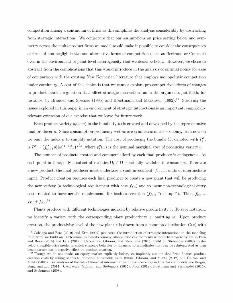
competition among a continuum of firms as this simplifies the analysis considerably by abstracting

from strategic interactions. We conjecture that our assumptions on price setting below and sym-

metry across the multi-product firms we model would make it possible to consider the consequences

of firms of non-negligible size and alternative forms of competition (such as Bertrand or Cournot)

even in the environment of plant-level heterogeneity that we describe below. However, we chose to

abstract from the complications that this would introduce in the analysis of optimal policy for ease

of comparison with the existing New Keynesian literature that employs monopolistic competition

under continuity. A cost of this choice is that we cannot explore pro-competitive effects of changes

in product market regulation that affect strategic interactions as in the arguments put forth, for

instance, by Brander and Spencer (1985) and Horstmann and Markusen (1992).17 Studying the

issues explored in this paper in an environment of strategic interactions is an important, empirically

relevant extension of our exercise that we leave for future work.

Each product variety ( ) in the bundle () is created and developed by the representative

final producer . Since consumption-producing sectors are symmetric in the economy, from now on

we omit the index to simplify notation. The cost of producing the bundle , denoted with ,

is =

¡R∞∈Ω

()

1−¢ 11− , where

() is the nominal marginal cost of producing variety .

The number of products created and commercialized by each final producer is endogenous. At

each point in time, only a subset of varieties Ω ⊂ Ω is actually available to consumers. To createa new product, the final producer must undertake a sunk investment, , in units of intermediate

input. Product creation requires each final producer to create a new plant that will be producing

the new variety (a technological requirement with cost ) and to incur non-technological entry

costs related to bureaucratic requirements for business creation (, “red tape”). Thus, ≡ + .

18

Plants produce with different technologies indexed by relative productivity . To save notation,

we identify a variety with the corresponding plant productivity , omitting . Upon product

creation, the productivity level of the new plant is drawn from a common distribution () with

17Colciago and Etro (2010) and Etro (2009) pioneered the introduction of strategic interactions in the modeling

framework we build on. Extensions to closed-economy, sticky-price environments without heterogeneity are in Etro

and Rossi (2015) and Faia (2012). Cacciatore, Ghironi, and Stebunovs (2015) build on Stebunovs (2008) to de-

velop a flexible-price model in which strategic behavior by financial intermediaries that can be reinterpreted as firm

headquarters has a negative effect on product creation.18Though we do not model an equity market explicitly below, we implicitly assume that firms finance product

creation costs by selling shares to domestic households as in Bilbiie, Ghironi, and Melitz (2012) and Ghironi and

Melitz (2005). For analyses of the role of financial intermediaries in producer entry in this class of models, see Bergin,

Feng, and Lin (2014), Cacciatore, Ghironi, and Stebunovs (2015), Notz (2012), Poutineau and Vermandel (2015),

and Stebunovs (2008).

9

support on [min∞). Foreign plants draw productivity levels from an identical distribution. This

relative productivity level remains fixed thereafter. Each plant uses intermediate input to produce

its differentiated product variety, with real marginal cost ≡ () = .

At time , each final Home producer commercializes varieties and creates new products

that will be available for sale at time + 1. New and incumbent plants can be hit by a “death”

shock with probability ∈ (0 1) at the end of each period. Therefore, the law of motion for thestock of producing plants is +1 = (1− )( +).

When serving the Foreign market, each final producer faces per-unit iceberg trade costs, 1,

and fixed export costs, . Fixed export costs are denominated in units of intermediate input

and paid for each exported product variety. Thus, the total fixed cost is ≡ , where

denotes the number of product varieties exported to Foreign. Absent fixed export costs, each

producer would find it optimal to sell all its product varieties in both countries. Fixed export costs

imply that only varieties produced by plants with sufficiently high productivity (above a cutoff

level determined by a zero-export-profit condition below) are exported. The share of exporting

plants is given by = [1−()].

Define two special “average” productivity levels (weighted by relative output shares): an average

for all producing plants and an average for all plants that export:

≡∙Z ∞

min

−1()¸ 1−1

≡∙

1

1−()

¸"Z ∞

−1()

# 1−1

(7)

These averages summarize all the information on the productivity distributions relevant for all

macroeconomic variables. Assume that (·) is Pareto with shape parameter − 1. As aresult, =

1(−1)min and =

1(−1), where ≡ ( − + 1). The share of exporting

plants is given by:

= [1−()] =

µmin

¶

−1 =

µmin

¶

(8)

Output bundles for domestic and export sale, and associated unit costs, are:

=

∙Z ∞

min

()−1 ()

¸ −1

, =

"Z ∞

()−1 ()

# −1

(9)

10

=

∙Z ∞

min

()

1−()¸ 11−

, =

"Z ∞

()

−1 ()

# 11−

(10)

In deciding how many products to create and which ones to export, the firm chooses the

sequences +1∞= and ∞= to minimize the intertemporal cost function:

( ∞X=

"

+

+

µ+1

1− −

¶ +

#) (11)

taking into account that = (min) ,

=

11− ,

=

11− ,

and = 1(−1)

. The first-order condition with respect to +1 yields the Euler equation

for product creation:

=

⎧⎪⎨⎪⎩(1− )+1

⎡⎢⎣ 1−1

µ+1

+1

+1+1+

+1+1

+1+1

+1

+1 +1

¶−+1

+1+1+1 + +1+1

⎤⎥⎦⎫⎪⎬⎪⎭ (12)

At the optimum, the cost of producing an additional variety (in units of consumption), , must

be equal to its expected benefit: the expected discounted marginal revenue from commercializing

the variety, net of export costs if it is exported, and the expected saving on future product creation

costs.

The first-order condition with respect to yields:

− ( − 1)( − 1)

= (13)

At the optimum, the marginal revenue from adding a variety with productivity to the export

bundle must be equal to the fixed export cost. Thus, varieties produced by plants with productivity

below are distributed only in the domestic market.

We are now left with the determination of domestic and export prices. Price setting happens

at the level of the bundles and rather than the level of individual varieties (or product

features). As shown in Cacciatore and Ghironi (2012), this preserves the aggregation properties of

the Melitz (2003) trade model in an environment of sticky prices.

Denote with the price (in Home currency) of the product bundle and let be the price

(in Foreign currency) of the exported bundle . Each final producer faces the following domestic

and foreign demand for its product bundles: = ()−

and = (∗ )− ∗

,

11

where and ∗

are aggregate demands of the consumption baskets in Home and Foreign.

Aggregate demand in each country includes sources other than household consumption, but it takes

the same form as the consumption basket, with the same elasticity of substitution 1 across

sectoral bundles. This ensures that the consumption price index for the consumption aggregator is

also the price index for aggregate demand of the basket.

We assume producer currency pricing (PCP): Each final producer sets and the domestic

currency price of the export bundle, , letting the price in the foreign market be =

,

where is the nominal exchange rate (units of Home currency per unit of Foreign). Absent fixed

export costs, the producer would set a single price , and the law of one price (adjusted for

the presence of iceberg trade costs) would determine the export price as = . With

fixed export costs, however, the composition of domestic and export bundles is different, and the

marginal costs of producing these bundles are not equal. Therefore, final producers choose two

different prices for the Home and Foreign markets even under PCP.

We assume that prices in the final sector are sticky: Final producers must pay quadratic price

adjustment costs as in Rotemberg (1982) when changing domestic and export prices. The nominal

costs of adjusting domestic and export price are, respectively, Γ ≡ 22, and Γ ≡

2

2, where ≥ 0 determines the size of the adjustment costs (domestic and export

prices are flexible if = 0), = (−1) − 1 and =¡

−1

¢ − 1. In Bilbiie,Ghironi, and Melitz (2008a), where price rigidity is at the level of individual product varieties, the

Rotemberg model of price stickiness simplifies the analysis considerably relative to the Calvo (1983)-

Yun (1996) approach.19 Since we impose price rigidity at the bundle level, using the Calvo-Yun

model would not imply the intractability that would arise from trying to use it at the variety level

in an environment with heterogeneity. However, we use the Rotemberg model of price stickiness

for consistency with the form of nominal rigidity we introduced in wage setting, where we were

constrained by tractability, and to facilitate comparison of results and intuitions with other work

on optimal monetary policy in this class of models that uses the same setup.20

When choosing and , the firm maximizes:

19Cavallari (2013) uses the Calvo-Yun model in her two-country version of Bilbiie-Ghironi-Melitz. Etro and Rossi

(2015) use Calvo-Yun in a version of Bilbiie-Ghironi-Melitz with Bertrand competition.20This work includes Bergin and Corsetti (2014), Faia (2012), and our own work in Bilbiie, Fujiwara, and Ghironi

(2014), Cacciatore and Ghironi (2012), and Cacciatore, Fiori, and Ghironi (2013). Much New Keynesian literature

on Ramsey-optimal monetary policy in models without producer entry builds on the Rotemberg model of nominal

rigidity in wages and/or prices. For instance, Arseneau and Chugh (2008), Chugh (2006), and Schmitt-Grohé and

Uribe (2004).

12

( ∞X=

"Ã

−

! −

Ã

−

! −

Γ

− Γ

#) (14)

subject to the demand schedules = ()−

and =£ ()

¤− ∗ where

≡ ∗ is the consumption-based real exchange rate (units of Home consumption per unit

of Foreign).

The profit-maximizing real price of Home output for domestic sale is given by:

=

(− 1)Ξ

(15)

where Ξ is given by:

Ξ ≡ 1−

22 +

(− 1)

( (1 + )−

"+1+1

(1 + +1)2

1 + +1

+1

#) (16)

Price stickiness introduces endogenous markup variation. The cost of adjusting prices gives firms

an incentive to change their markups over time in order to smooth price changes across periods.

When prices are flexible ( = 0), the markup is constant and equal to (− 1).21

The real price (relative to the Foreign price index) of Home export output implied by the

optimal choice of is equal to:

∗=

(− 1)Ξ

(17)

where:

Ξ ≡ 1−

2

2

+

(− 1)

(

³1 +

´−

"+1

+1

¡1 + +1

¢21 + +1

+1

#) (18)

Absent fixed export costs = min and Ξ = Ξ.

As noted above, the assumption of price rigidity at the level of the sectoral output bundles

and rather than the individual product varieties () and () allows us to introduce price

stickiness in the Ghironi-Melitz (2005) framework while still preserving the aggregation properties

21The assumption of C.E.S. preferences over a continuum of products implies that the model does not capture

pro-competitive effects of product market reforms via flexible-price markup variation. See Cacciatore and Fiori

(2010) and Cacciatore, Fiori, and Ghironi (2013) for models that incorporate such mechanism by assuming a translog

expenditure function.

13

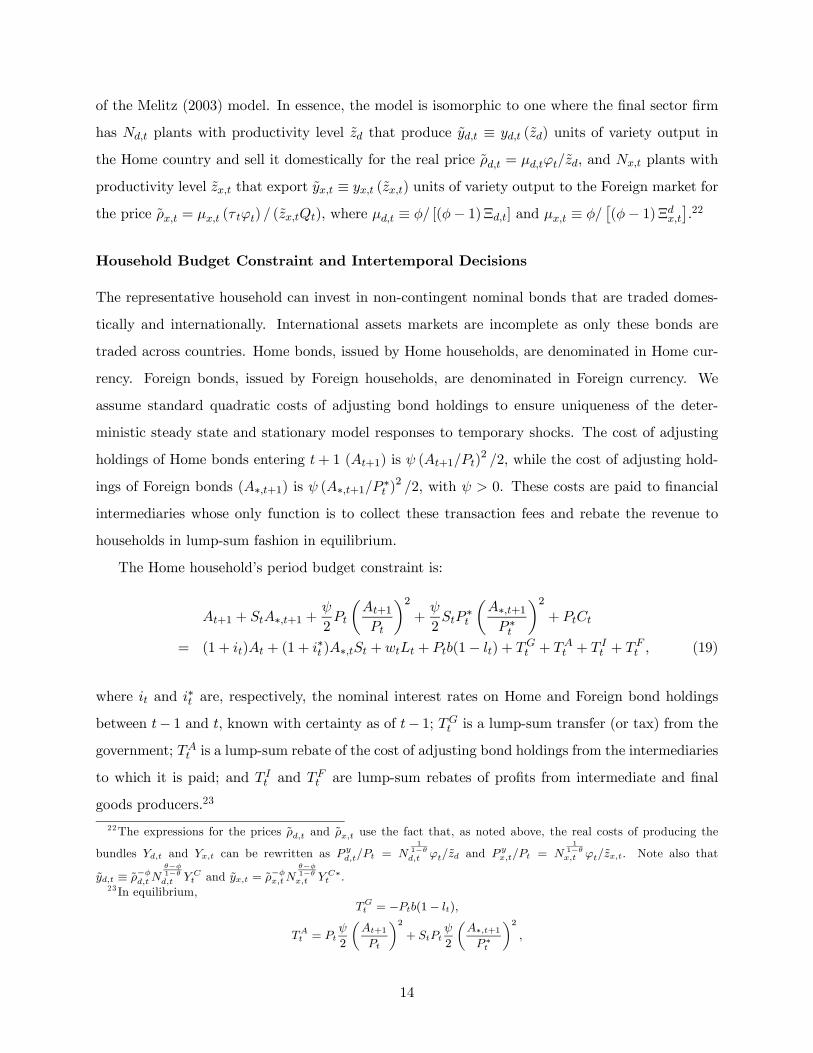
of the Melitz (2003) model. In essence, the model is isomorphic to one where the final sector firm

has plants with productivity level that produce ≡ () units of variety output in

the Home country and sell it domestically for the real price = , and plants with

productivity level that export ≡ () units of variety output to the Foreign market for

the price = ( ) (), where ≡ [(− 1)Ξ] and ≡ £(− 1)Ξ

¤.22

Household Budget Constraint and Intertemporal Decisions

The representative household can invest in non-contingent nominal bonds that are traded domes-

tically and internationally. International assets markets are incomplete as only these bonds are

traded across countries. Home bonds, issued by Home households, are denominated in Home cur-

rency. Foreign bonds, issued by Foreign households, are denominated in Foreign currency. We

assume standard quadratic costs of adjusting bond holdings to ensure uniqueness of the deter-

ministic steady state and stationary model responses to temporary shocks. The cost of adjusting

holdings of Home bonds entering + 1 (+1) is (+1)2 2, while the cost of adjusting hold-

ings of Foreign bonds (∗+1) is (∗+1 ∗ )2 2, with 0. These costs are paid to financial

intermediaries whose only function is to collect these transaction fees and rebate the revenue to

households in lump-sum fashion in equilibrium.

The Home household’s period budget constraint is:

+1 + ∗+1 +

2

µ+1

¶2+

2

∗

µ∗+1 ∗

¶2+

= (1 + ) + (1 + ∗ )∗ + + (1− ) + +

+ +

(19)

where and ∗ are, respectively, the nominal interest rates on Home and Foreign bond holdings

between − 1 and , known with certainty as of − 1; is a lump-sum transfer (or tax) from the

government; is a lump-sum rebate of the cost of adjusting bond holdings from the intermediaries

to which it is paid; and and

are lump-sum rebates of profits from intermediate and final

goods producers.23

22The expressions for the prices and use the fact that, as noted above, the real costs of producing the

bundles and can be rewritten as =

11− and

=

11− . Note also that

≡ −

−1−

and = −

−1− ∗

.23 In equilibrium,

= −(1− )

=

2

+1

2+

2

∗+1 ∗

2

14

Let +1 ≡ +1 denote real holdings of Home bonds (in units of Home consumption) and

let ∗+1 ≡ ∗+1 ∗ denote real holdings of Foreign bonds (in units of Foreign consumption).

The Euler equations for bond holdings are:

1++1 = (1++1)

µ+1

1 + +1

¶ (20)

1 + ∗+1 =¡1 + ∗+1

¢

⎡⎣+1 +1

³1 + ∗+1

´⎤⎦ (21)

where ≡ (−1)− 1 and ∗+1 ≡¡ ∗ ∗−1

¢− 1.Details of the equilibrium of our model economy are in Cacciatore and Ghironi (2012). We limit

ourselves to presenting the law of motion for net foreign assets below.

Net Foreign Assets and the Trade Balance

Bonds are in zero net supply, which implies the equilibrium conditions +1+∗+1 = 0 and ∗∗+1+

∗+1 = 0 in all periods. Cacciatore and Ghironi (2012) show that imposing equilibrium conditions

on the budget constraints of the representative Home and Foreign households and subtracting the

constraint for the Foreign household (expressed in units of Home consumption) from that for the

Home household yields the following law of motion for Home net foreign assets:

+1 +∗+1 =1 +

1 + +

1 + ∗1 + ∗

∗ + −∗

∗

∗ (22)

In addition to equilibrium in bond markets, the budget constraints of Home and Foreign govern-

ments, and the rebates received by households, this equation accounts for the fact that demand

for consumption output comes from several sources and for labor market equilibrium in each coun-

try. For instance, Home consumption demand aggregates household consumption, costs of vacancy

posting in the labor market, costs of wage adjustment in the intermediate sector, and costs of price

=

−

− −

22

=

− 1

−

22

+

− 1

−

2

2 − ( +)

15

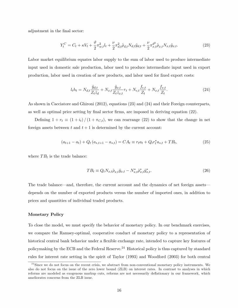
adjustment in the final sector:

= + +

22 +

22 +

2

2

(23)

Labor market equilibrium equates labor supply to the sum of labor used to produce intermediate

input used in domestic sale production, labor used to produce intermediate input used in export

production, labor used in creation of new products, and labor used for fixed export costs:

=

+

+

+

(24)

As shown in Cacciatore and Ghironi (2012), equations (23) and (24) and their Foreign counterparts,

as well as optimal price setting by final sector firms, are imposed in deriving equation (22).

Defining 1 + ≡ (1 + ) (1 + ), we can rearrange (22) to show that the change in net

foreign assets between and + 1 is determined by the current account:

(+1 − ) + (∗+1 − ∗) = ≡ +∗ ∗ + (25)

where is the trade balance:

≡ −∗

∗

∗ (26)

The trade balance–and, therefore, the current account and the dynamics of net foreign assets–

depends on the number of exported products versus the number of imported ones, in addition to

prices and quantities of individual traded products.

Monetary Policy

To close the model, we must specify the behavior of monetary policy. In our benchmark exercises,

we compare the Ramsey-optimal, cooperative conduct of monetary policy to a representation of

historical central bank behavior under a flexible exchange rate, intended to capture key features of

policymaking by the ECB and the Federal Reserve.24 Historical policy is thus captured by standard

rules for interest rate setting in the spirit of Taylor (1993) and Woodford (2003) for both central

24Since we do not focus on the recent crisis, we abstract from non-conventional monetary policy instruments. We

also do not focus on the issue of the zero lower bound (ZLB) on interest rates. In contrast to analyses in which

reforms are modeled as exogenous markup cuts, reforms are not necessarily deflationary in our framework, which

ameliorates concerns from the ZLB issue.

16

banks in our model.

As discussed in Cacciatore and Ghironi (2012), the specification of historical policy rules for

the central banks requires us to define data-consistent price and quantity variables in our model:

Endogenous product creation and “love for variety” in preferences imply that variables measured in

units of consumption do not have a direct counterpart in the data, i.e., they are not data-consistent.

As the economy experiences entry of Home and Foreign products, the welfare-consistent aggregate

price index can fluctuate even if product prices remain constant. In the data, however, aggregate

price indexes do not take these variety effects into account.25 We follow Ghironi and Melitz (2005)

and construct an average price index ≡¡ +∗

¢ 1−1 . The average price index is closer

to the actual CPI data constructed by statistical agencies than the welfare-based index , and,

therefore, it is the data-consistent CPI implied by the model. In turn, given any variable in

units of consumption, its data-consistent counterpart can be obtained as ≡ .

Under the historical characterization of policy, we assume that the exchange rate is flexible, and

each country’s central bank sets its interest rate to respond to data-consistent CPI inflation and

GDP gap relative to the equilibrium with flexible prices and wages:

1 + +1 = (1 + )h(1 + ) (1 + )

³

´ i1− 0 ≤ ≤ 1, 0, ≥ 0, (27)

where is the data-consistent CPI inflation and is the data-consistent GDP gap.

26 A similar

rule for interest rate setting applies to the Foreign central bank. We compare the properties of our

model world economy under this international monetary regime to those generated by Ramsey-

optimal, cooperative monetary policy chosen by a worldwide Ramsey authority that maximizes an

equally weighted average of Home and Foreign welfare.27

25There is much empirical evidence that gains from variety are mostly unmeasured in CPI data, as documented

for instance by Broda and Weinstein (2010).26We define GDP, denoted with , as total income: the sum of labor income and profit income from final and

intermediate producers. Formally, ≡ () + +

. We define the GDP gap as ≡

where

is data-consistent GDP under flexible prices and wages.27See the Appendix for details. Cacciatore and Ghironi (2012) consider also the case in which Home and Foreign

Ramsey-central banks act in non-cooperative fashion. With high trade integration, welfare gains from cooperation are

small relative to non-cooperative Ramsey policies, but they are larger relative to historical policy, as trade amplifies

spillovers from non-optimized policies. Following Sims (2007), we focus on historical behavior as the empirically

relevant benchmark here. Results for the non-cooperative Ramsey scenario are available on request.

17

3 Sources of Inefficiency

The worldwide Ramsey planner that determines the optimal, cooperative monetary policy uses

its policy instruments (the Home and Foreign interest rates) to address the consequences of a set

of distortions that exist in the market economy of our model. To understand these distortions

and the tradeoffs they create for policy, Cacciatore and Ghironi (2012) compare the equilibrium

conditions of the market economy to those implied by the solution to the first-best, optimal planning

problem. This makes it possible to define inefficiency wedges for the market economy (relative to

the social planner’s optimum) and describe Ramsey policy in terms of its implications for these

wedges. In this section, we summarize the sources of inefficiency in our model with reference to

the margins of economic adjustment on which they impinge. Specifically, price and wage stickiness,

firm monopoly power, unemployment benefits, “red tape” regulation, trade costs, and incomplete

markets affect five margins of adjustment and the resource constraint for consumption output in

the market economy:

• Product creation margin: Sticky prices result in inefficient time-variation and lack of

synchronization of domestic and export markups that introduce inefficiency in the product

creation margin (described by the Euler equations for product creation at Home and abroad).

Time variation and lack of synchronization of markups across markets imply inefficient devi-

ations of the monopoly profit incentive for product creation (the markup) from the welfare

benefit of product variety determined by the constant elasticity of substitution across prod-

ucts. Similarly, if steady-state inflation is not zero, sticky prices imply a departure from the

balancing of product creation incentives and welfare benefit of variety implied by continuous

Dixit-Stiglitz preferences under flexible prices. Finally, the product creation margin is affected

by the presence of the non-technological entry costs and of any non-technological, ineffi-

ciently set component of trade costs that affects the role of expected export profits in product

creation.28 As shown in Cacciatore and Ghironi (2012), the Euler equations for domestic and

foreign product creation coincide with those of the first-best environment when prices and

wages are flexible, there is no “red tape,” and trade costs are of purely technological nature.29

28Bilbiie, Ghironi, and Melitz (2008b) and Chugh and Ghironi (2015) consider the case = − and discussthe determination of optimal product creation subsidies in a first- or second-best environment, respectively. We will

focus on the consequences of an exogenous deregulation that reduces non-technological barriers to entry, abstracting

from the issue of optimal entry subsidies (or taxes). In the continuous Dixit-Stiglitz environment of this paper, it

would be optimal to set = 0 in the absence of other distortions.29Efficiency along the product creation margin in this case is a consequence of the assumption of a Dixit-Stiglitz

continuum. This implies that the monopoly profit incentive for product creation is perfectly aligned with the welfare

18

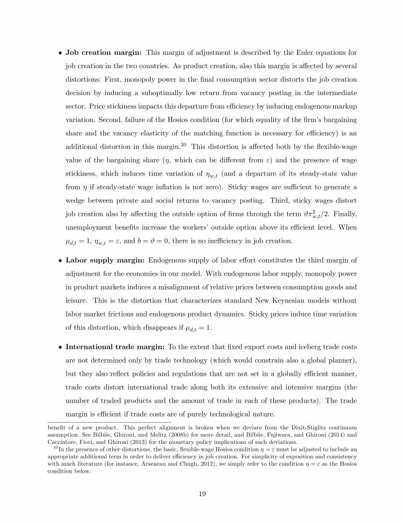
• Job creation margin: This margin of adjustment is described by the Euler equations forjob creation in the two countries. As product creation, also this margin is affected by several

distortions: First, monopoly power in the final consumption sector distorts the job creation

decision by inducing a suboptimally low return from vacancy posting in the intermediate

sector. Price stickiness impacts this departure from efficiency by inducing endogenous markup

variation. Second, failure of the Hosios condition (for which equality of the firm’s bargaining

share and the vacancy elasticity of the matching function is necessary for efficiency) is an

additional distortion in this margin.30 This distortion is affected both by the flexible-wage

value of the bargaining share (, which can be different from ) and the presence of wage

stickiness, which induces time variation of (and a departure of its steady-state value

from if steady-state wage inflation is not zero). Sticky wages are sufficient to generate a

wedge between private and social returns to vacancy posting. Third, sticky wages distort

job creation also by affecting the outside option of firms through the term 22. Finally,

unemployment benefits increase the workers’ outside option above its efficient level. When

= 1, = , and = = 0, there is no inefficiency in job creation.

• Labor supply margin: Endogenous supply of labor effort constitutes the third margin ofadjustment for the economies in our model. With endogenous labor supply, monopoly power

in product markets induces a misalignment of relative prices between consumption goods and

leisure. This is the distortion that characterizes standard New Keynesian models without

labor market frictions and endogenous product dynamics. Sticky prices induce time variation

of this distortion, which disappears if = 1.

• International trade margin: To the extent that fixed export costs and iceberg trade costsare not determined only by trade technology (which would constrain also a global planner),

but they also reflect policies and regulations that are not set in a globally efficient manner,

trade costs distort international trade along both its extensive and intensive margins (the

number of traded products and the amount of trade in each of these products). The trade

margin is efficient if trade costs are of purely technological nature.

benefit of a new product. This perfect alignment is broken when we deviate from the Dixit-Stiglitz continuum

assumption. See Bilbiie, Ghironi, and Melitz (2008b) for more detail, and Bilbiie, Fujiwara, and Ghironi (2014) and

Cacciatore, Fiori, and Ghironi (2013) for the monetary policy implications of such deviations.30 In the presence of other distortions, the basic, flexible-wage Hosios condition = must be adjusted to include an

appropriate additional term in order to deliver efficiency in job creation. For simplicity of exposition and consistency

with much literature (for instance, Arseneau and Chugh, 2012), we simply refer to the condition = as the Hosios

condition below.

19

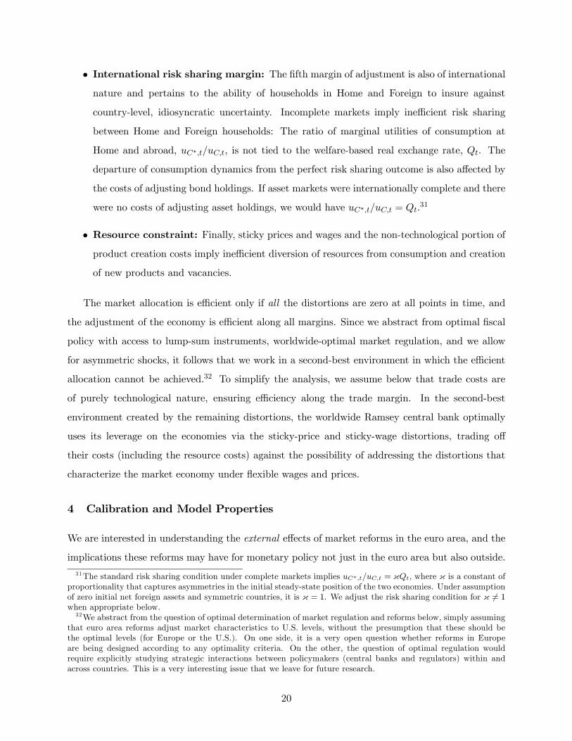
• International risk sharing margin: The fifth margin of adjustment is also of internationalnature and pertains to the ability of households in Home and Foreign to insure against

country-level, idiosyncratic uncertainty. Incomplete markets imply inefficient risk sharing

between Home and Foreign households: The ratio of marginal utilities of consumption at

Home and abroad, ∗, is not tied to the welfare-based real exchange rate, . The

departure of consumption dynamics from the perfect risk sharing outcome is also affected by

the costs of adjusting bond holdings. If asset markets were internationally complete and there

were no costs of adjusting asset holdings, we would have ∗ = .31

• Resource constraint: Finally, sticky prices and wages and the non-technological portion ofproduct creation costs imply inefficient diversion of resources from consumption and creation

of new products and vacancies.

The market allocation is efficient only if all the distortions are zero at all points in time, and

the adjustment of the economy is efficient along all margins. Since we abstract from optimal fiscal

policy with access to lump-sum instruments, worldwide-optimal market regulation, and we allow

for asymmetric shocks, it follows that we work in a second-best environment in which the efficient

allocation cannot be achieved.32 To simplify the analysis, we assume below that trade costs are

of purely technological nature, ensuring efficiency along the trade margin. In the second-best

environment created by the remaining distortions, the worldwide Ramsey central bank optimally

uses its leverage on the economies via the sticky-price and sticky-wage distortions, trading off

their costs (including the resource costs) against the possibility of addressing the distortions that

characterize the market economy under flexible wages and prices.

4 Calibration and Model Properties

We are interested in understanding the external effects of market reforms in the euro area, and the

implications these reforms may have for monetary policy not just in the euro area but also outside.

31The standard risk sharing condition under complete markets implies ∗ = κ, where κ is a constant ofproportionality that captures asymmetries in the initial steady-state position of the two economies. Under assumption

of zero initial net foreign assets and symmetric countries, it is κ = 1. We adjust the risk sharing condition for κ 6= 1when appropriate below.32We abstract from the question of optimal determination of market regulation and reforms below, simply assuming

that euro area reforms adjust market characteristics to U.S. levels, without the presumption that these should be

the optimal levels (for Europe or the U.S.). On one side, it is a very open question whether reforms in Europe

are being designed according to any optimality criteria. On the other, the question of optimal regulation would

require explicitly studying strategic interactions between policymakers (central banks and regulators) within and

across countries. This is a very interesting issue that we leave for future research.

20

For this reason, we take the United States as reference point for our benchmark calibration, and

for an initial investigation of our model’s properties. We perform this investigation by calibrating

both countries in our model symmetrically to U.S. targets, and studying the ability of the model to

replicate standard moments of the U.S. business cycle and its international interdependence with

foreign fluctuations.33 To build intuition for the mechanisms at work, we discuss the responses to

a Home productivity shock.

Calibration

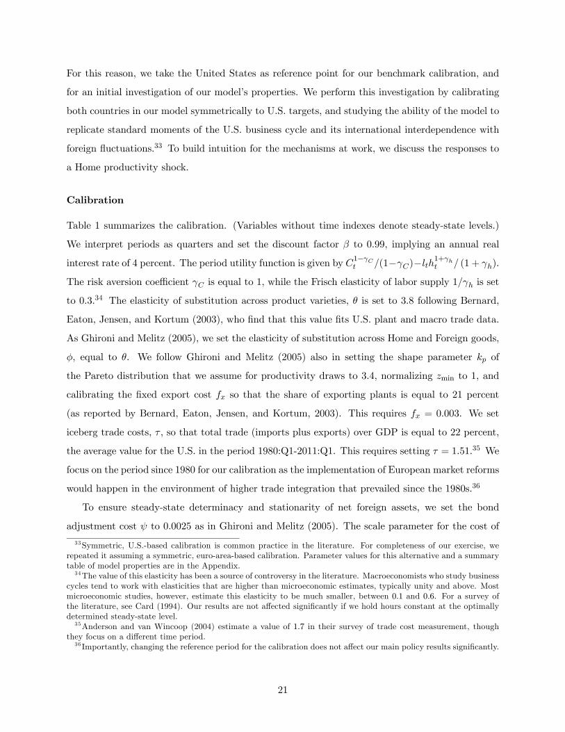
Table 1 summarizes the calibration. (Variables without time indexes denote steady-state levels.)

We interpret periods as quarters and set the discount factor to 099, implying an annual real

interest rate of 4 percent. The period utility function is given by 1− (1−)−1+ (1 + ).

The risk aversion coefficient is equal to 1, while the Frisch elasticity of labor supply 1 is set

to 03.34 The elasticity of substitution across product varieties, is set to 38 following Bernard,

Eaton, Jensen, and Kortum (2003), who find that this value fits U.S. plant and macro trade data.

As Ghironi and Melitz (2005), we set the elasticity of substitution across Home and Foreign goods,

, equal to . We follow Ghironi and Melitz (2005) also in setting the shape parameter of

the Pareto distribution that we assume for productivity draws to 34, normalizing min to 1, and

calibrating the fixed export cost so that the share of exporting plants is equal to 21 percent

(as reported by Bernard, Eaton, Jensen, and Kortum, 2003). This requires = 0003. We set

iceberg trade costs, , so that total trade (imports plus exports) over GDP is equal to 22 percent,

the average value for the U.S. in the period 1980:Q1-2011:Q1. This requires setting = 151.35 We

focus on the period since 1980 for our calibration as the implementation of European market reforms

would happen in the environment of higher trade integration that prevailed since the 1980s.36

To ensure steady-state determinacy and stationarity of net foreign assets, we set the bond

adjustment cost to 00025 as in Ghironi and Melitz (2005). The scale parameter for the cost of

33Symmetric, U.S.-based calibration is common practice in the literature. For completeness of our exercise, we

repeated it assuming a symmetric, euro-area-based calibration. Parameter values for this alternative and a summary

table of model properties are in the Appendix.34The value of this elasticity has been a source of controversy in the literature. Macroeconomists who study business

cycles tend to work with elasticities that are higher than microeconomic estimates, typically unity and above. Most

microeconomic studies, however, estimate this elasticity to be much smaller, between 01 and 06. For a survey of

the literature, see Card (1994). Our results are not affected significantly if we hold hours constant at the optimally

determined steady-state level.35Anderson and van Wincoop (2004) estimate a value of 17 in their survey of trade cost measurement, though

they focus on a different time period.36 Importantly, changing the reference period for the calibration does not affect our main policy results significantly.

21

adjusting prices, , is equal to 80, close to the value used in Bilbiie, Ghironi, and Melitz (2008a)

and estimated for the U.S. by Ireland (2001). Parameter values in this range are consistent with

the degree of price rigidity often assumed in models that adopt the framework of Calvo (1983) and

Yun (1996). We choose , the scale parameter of nominal wage adjustment costs, so that the model

reproduces the volatility of unemployment relative to GDP observed in the period 1980:Q1-2011:Q1

used to calibrate iceberg trade costs. This implies = 80 too.37 To calibrate the total entry costs,

we follow Ebell and Haefke (2009) and set so that entry costs amount to 52 months of per capita

output. This implies = 058.

We set unemployment benefits, , to 019, so that the replacement rate, (), is 055, as

reported by OECD (2004).38 The flexible-wage bargaining share of workers, 1 − , is equal to

04, as estimated by Flinn (2006). The elasticity of the matching function, , is equal to 06,

as estimated by Blanchard and Diamond (1989) and such that the Hosios condition holds in a

steady state with zero inflation. The exogenous separation rate between firms and workers, , is

10 percent, as reported by Shimer (2005). To pin down exogenous producer exit, , we target the

40-percent portion of worker separation due to plant exit documented by Haltiwanger, Scarpetta,

and Schweiger (2008). This yields = 0029, a value very close to that in Ghironi and Melitz

(2005).

Two labor market parameters are left for calibration: the scale parameter for the cost of vacancy

posting, , and the matching efficiency parameter, . We calibrate these parameters to match the

average probability of finding a job and the probability of filling a vacancy in the period 1980:Q1-

2011:Q1. The former is 60 percent, while the latter is 70 percent, in line with Shimer (2005). This

implies = 010 and = 073.39 With this calibration, the model generates an 11-percent steady-

state unemployment rate, which is not distant from the U.S. average plus a plausible adjustment

for job searchers not included in unemployment rate statistics.

For the bivariate productivity process in the intermediate sector, we set persistence and spillover

parameters (respectively, the diagonal and off-diagonal parameters in the autoregressive matrix

coefficient) consistent with evidence in Baxter (1995) and Baxter and Farr (2005), implying persis-

tence equal to 0999 and zero spillovers across countries. Moreover, we set the standard deviation

37Changing the reference period for the calibration of this parameter does not change the parameter value signifi-

cantly, and the implied changes have very little effects on the properties of the model.38Our calibration implies that the overall flow value of unemployment, () + , relative to the worker’s

compensation, , is 75 percent.39As for the wage rigidity parameter, changing the reference period implies little changes in these values, and little

effects on the properties of the model.

22

of productivity innovations at 0008 to match the absolute volatility of U.S. GDP in the period

1980:Q1-2011:Q1, but we leave the correlation of innovations at the standard 0258 of Baxter (1995)

and Backus, Kehoe, and Kydland (1992, 1994).

Finally, the parameter values in the historical rule for interest rate setting by the Federal

Reserve are those estimated by Clarida, Galí, and Gertler (2000). The inflation and GDP gap

coefficients are 162 and 034, respectively, and the smoothing parameter is 071. These values are

quite representative also of later literature that estimated interest rate reaction functions for the

Federal Reserve (and the central banks of other low inflation countries) for the period since the

early 1980s.

Impulse Responses

Figure 1 shows impulse responses to a one-percent positive innovation to Home productivity under

historical interest rate setting for both central banks in the model. We assume shock persistence

09 for this figure as this facilitates the presentation of results relative to the extremely slow return

to the steady state implied by persistence 0999. Focus on the Home country first. Unemployment

() does not respond on impact, but it falls in the periods after the shock. The higher expected

return of a match induces domestic intermediate input producers to post more vacancies on impact,

which results in higher employment in the following period. Firms and workers (costly) renegotiate

nominal wages because of the higher surplus generated by existing matches, and wage inflation

() increases.40

Employment and labor income rise in the more productive economy, boosting aggregate de-

mand for final goods and household consumption (). The larger present discounted value of

future profits generates higher expected return to product creation, stimulating product creation

() and investment ( ≡ , not shown) at Home. The number of domestic plants that

produce for the export market also increases, since higher aggregate productivity reduces the export

productivity cutoff (not shown).

Foreign households shift resources to Home to finance product creation in the more produc-

tive economy. Home initially runs a current account deficit to finance increased product creation

( falls on impact), and Foreign households share the benefit of higher Home productivity by

shifting resources to Home via lending. (Home’s deficit becomes more persistent if we increase the

40Wage adjustment costs make the effective firm’s bargaining power procyclical, i.e., (not shown) rises. Other

things equal, the increase in dampens the response of the renegotiated equilibrium wage, amplifying the response

of job creation to the shock.

23

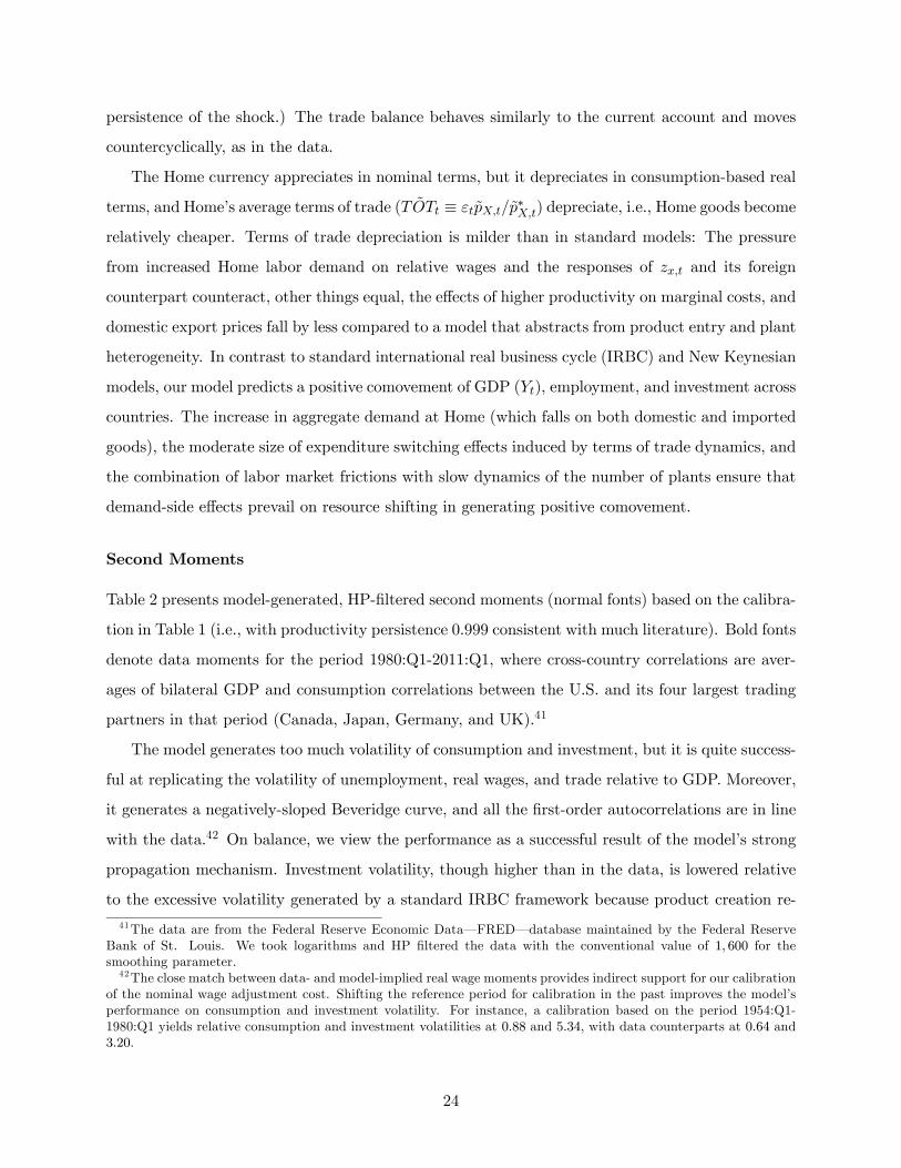
persistence of the shock.) The trade balance behaves similarly to the current account and moves

countercyclically, as in the data.

The Home currency appreciates in nominal terms, but it depreciates in consumption-based real

terms, and Home’s average terms of trade ( ≡ ∗) depreciate, i.e., Home goods become

relatively cheaper. Terms of trade depreciation is milder than in standard models: The pressure

from increased Home labor demand on relative wages and the responses of and its foreign

counterpart counteract, other things equal, the effects of higher productivity on marginal costs, and

domestic export prices fall by less compared to a model that abstracts from product entry and plant

heterogeneity. In contrast to standard international real business cycle (IRBC) and New Keynesian

models, our model predicts a positive comovement of GDP (), employment, and investment across

countries. The increase in aggregate demand at Home (which falls on both domestic and imported

goods), the moderate size of expenditure switching effects induced by terms of trade dynamics, and

the combination of labor market frictions with slow dynamics of the number of plants ensure that

demand-side effects prevail on resource shifting in generating positive comovement.

Second Moments

Table 2 presents model-generated, HP-filtered second moments (normal fonts) based on the calibra-

tion in Table 1 (i.e., with productivity persistence 0999 consistent with much literature). Bold fonts

denote data moments for the period 1980:Q1-2011:Q1, where cross-country correlations are aver-

ages of bilateral GDP and consumption correlations between the U.S. and its four largest trading

partners in that period (Canada, Japan, Germany, and UK).41

The model generates too much volatility of consumption and investment, but it is quite success-

ful at replicating the volatility of unemployment, real wages, and trade relative to GDP. Moreover,

it generates a negatively-sloped Beveridge curve, and all the first-order autocorrelations are in line

with the data.42 On balance, we view the performance as a successful result of the model’s strong

propagation mechanism. Investment volatility, though higher than in the data, is lowered relative

to the excessive volatility generated by a standard IRBC framework because product creation re-

41The data are from the Federal Reserve Economic Data–FRED–database maintained by the Federal Reserve

Bank of St. Louis. We took logarithms and HP filtered the data with the conventional value of 1 600 for the

smoothing parameter.42The close match between data- and model-implied real wage moments provides indirect support for our calibration

of the nominal wage adjustment cost. Shifting the reference period for calibration in the past improves the model’s

performance on consumption and investment volatility. For instance, a calibration based on the period 1954:Q1-

1980:Q1 yields relative consumption and investment volatilities at 088 and 534, with data counterparts at 064 and

320.

24

quires hiring new workers. This process is time consuming due to search and matching frictions in

the labor market, dampening investment dynamics. In contrast, consumption is more volatile than

the excessive smoothness of traditional models as shocks induce larger and longer-lasting income

effects.

With respect to the international dimension of the business cycle, the model is quite successful

in matching the cyclical properties of trade data: exports () and imports () are more

volatile than GDP, the trade balance is countercyclical, and its volatility is in line with the data.

These stylized facts are not reproduced by standard IRBC models (see Engel and Wang, 20011) and

many New Keynesian models. The model can also reproduce a ranking of cross-country correlations

that is a challenge for standard IRBC models: GDP correlation across countries is larger than

consumption correlation.43 As shown in Figure 1, an increase in Home productivity generates

Foreign expansion through trade linkages, as demand-side complementarities more than offset the

effect of resource shifting to the more productive economy. (This is true also with higher shock

persistence than for the example of Figure 1.) Moreover, absent technology spillovers, Foreign

consumers have weaker incentives to increase consumption on impact, which reduces the cross-

country consumption correlation.44

5 Market Reforms and Monetary Policy in the International Economy

Having established that the model successfully reproduces (qualitatively and/or quantitatively)

several features of the international business cycle, we turn to our main exercise and study the

domestic and international consequences of market reforms in one of the countries in our model,

and how such reforms affect the conduct of optimal monetary policy.

We calibrated both countries in the model to U.S. targets to assess the model’s properties. A

goal of our exercise in this paper is to begin shedding light on how market reforms in Europe are

likely to affect transatlantic interdependence and policy incentives for the Federal Reserve and the

ECB. For this purpose, we isolate structural conditions of product and labor markets as the only

source of asymmetry between the euro area and the United States in our model. We accomplish this

by re-calibrating the parameters that capture Home market regulation (the entry cost in product

43A calibration based on the pre-globalization, 1954:Q1-1980:Q1, period matches the cross-country correlation

of GDPs almost perfectly (a traditionally elusive result) while preserving the ranking of consumption and GDP

correlations. Details are available on request.44The very low correlation of consumption across countries in Table 2 is due to the combination of incomplete

markets, bond adjustment costs (albeit small), and extremely persistent shocks. Reducing shock persistence facilitates

risk sharing and increases consumption correlation, consistent with results in Baxter and Crucini (1995).

25

markets, ; unemployment benefits, ; and the flexible-wage bargaining power of workers, 1 − ,

taken as a measure of employment protection) to European levels (see the Appendix for details).45

This adjustment in parameter values allows us to treat the Home country as a model-euro area

that differs from the U.S. only by featuring more rigid product and labor markets, and to isolate

the consequences of this asymmetry and of reforms that align European market characteristics to

U.S. levels.

Under the new calibration, we compute the welfare benefit of moving from the historical policy

behavior of the calibration in Table 1 to the Ramsey-optimal cooperative monetary policy, as well

as the cooperative, Ramsey-optimal, long-run inflation rates in the two countries. These results

are reported in Table 3, in the “Status Quo” row. We then compute impulse responses to Home

product market reform (Figure 2), Home labor market reform (Figure 3), and joint reform of both

Home markets (Figure 4). Each Home market reform brings the relevant parameter value(s) to the

flexible (U.S.) level used in the previous section. The parameter change is treated as a permanent

shock, and the impulse responses trace the domestic and international effects of this change from

the impact period to the long run, under historical policy or the cooperative, Ramsey-optimal

policy.46

Since much of the policy debate on the benefits of market reforms focuses on the benefits they

would generate by reallocating resources to more efficient uses, for each reform, we also present

figures that make it possible to study such reallocation effects. Specifically, part b of Figures 2-4

shows the responses of three measures of productivity and employment across different uses of

resources in production. In our model economy, it is possible to define the productivity of the

average Home product-variety line, whose output is sold both domestically and abroad, as:

=

("−1 +

µ

¶−1

#) 1−1

(28)

45For our purposes, changing directly the value of is sufficient to capture changes in product market regulation.

The underlying assumption is that the change comes from a change in the “red tape” portion of the overall entry

cost rather than in the technological requirement .46 In the Ramsey policy problem for this exercise, we assume that the initial conditions are given by the rigid steady

state under the historical policy (which features zero inflation). In technical terms, we solve for the Ramsey-optimal

policy in response to market deregulation assuming time-zero commitment to the optimal plan. An alternative

approach would be to solve for the optimal response to reform assuming that the initial conditions are given by the

optimal Ramsey steady state with high product and labor market regulation, i.e., from a timeless perspective. Our

choice has the advantage of making the comparison between historical and Ramsey-optimal policy more transparent.

(In the presence of different initial conditions associated to alternative monetary policy regimes, as implied by the

alternative approach, it would be impossible to isolate the role of monetary policy for the transition dynamics following

reforms.)

26

The first row of each b-figure shows the responses to reform of this average productivity, of the aver-

age productivity of product lines that are sold only domestically (, which is constant by construc-

tion), and of the average productivity for export production (; this is the average productivity of

the export operation of product lines sold both domestically and abroad). We then exploit linearity

of production of differentiated varieties in the non-traded intermediate input, and linearity of pro-

duction of the latter in labor, to plot (in the second row of each b-figure) the responses of implicit

employment in the average production line, () () ≡ () ()+ () (), em-

ployment in the average product variety line that is sold only domestically, () (), and

employment in the average export operation of traded varieties, () (). These are im-

plicit measures of employment in production of the differentiated varieties, as our model assumes

that labor is used in production of the intermediate input. However, linearity of the production

process from labor to final varieties makes it possible for us to characterize transparently the use

of labor in variety production, and thus analyze the resource reallocation effects discussed by pol-

icymakers in the context of our model. (The bottom two rows in each b-figure show the same

variables for the Foreign country, to investigate the external resource allocation consequences of

Home market reforms.)

Finally, we address the welfare consequences of reforms in Tables 3 and 4. All welfare results are

in percentage of steady-state consumption. Table 3 presents the changes in welfare directly implied

by Home reforms under historical policy and the Ramsey-optimal policy.47 Table 4 presents the

effects of Home reforms on the welfare costs of business cycles.48

Optimal Policy in the Status Quo

As Table 3 shows, moving from historical policy to the Ramsey-optimal, cooperative policy increases

welfare by 054 percent of steady-state consumption at Home and 027 percent in Foreign under

the regulation status quo. The Ramsey-optimal policy implies a higher inflation rate in the Home

47Results for the case in which Home pegs the exchange rate of its currency against Foreign are available on request.

We do not include them in the paper given the extremely low likelihood that the ECB would ever peg the euro to

the dollar.48When studying optimal policy over the business cycle, we follow standard practice in the literature and assume

that the non-stochastic steady state is the same across the policy regimes we consider, and it is given by the Ramsey-

optimal steady state (which features non-zero inflation). When computing the welfare costs of business cycles,

we follow Schmitt-Grohé and Uribe (2007), and we focus on the conditional expected discounted utility of the

representative agent (as opposed to the unconditional one) in order to account for the transitional effects from the

deterministic to the stochastic steady state. Since the non-stochastic steady state is the same across the policy regimes

we consider, our choice of computing expected welfare conditional on the initial state being the non-stochastic steady

state ensures that the economy begins from the same initial point under all policies.

27

country than in Foreign. (In steady state, consumer and producer price inflation rates coincide, so

we simply refer to inflation when talking about the long-run target.) This can be understood with

reference to the distortions we discussed above: A long-run equilibrium with constant endogenous

variables eliminates some of these distortions: A constant markup removes the markup variation

distortion from the product creation margin; Constant consumption removes the risk-sharing dis-

tortion of incomplete markets, and constant, zero net foreign assets eliminate the effect of asset

adjustment costs. Monopoly power of firms in the downstream sector, positive unemployment

benefits, and a departure from the Hosios condition in Home imply suboptimally low job-creation.

Since = = , positive inflation raises firm bargaining power , favoring vacancy posting by

firms. The intuition for the positive relation between inflation and is straightforward: Positive

inflation is costly for firms, who bear the costs of wage adjustment. Suppose we want a firm to hire

the same amount of labor in an environment of positive inflation as it would with zero inflation.

For the firm to be willing to do that with positive wage adjustment costs, it must be compensated

by the willingness of workers to accept a lower level of the bargained wage. For this to happen, the

bargaining power of firms must rise.

Importantly, the result of a positive Ramsey inflation target is not an “automatic” consequence

of assuming a form of nominal rigidity that implies long-run non-neutrality of money. As shown

in Bilbiie, Fujiwara, and Ghironi (2014), the same form of price stickiness implies a zero Ramsey-

optimal inflation target in the sticky-price model of Bilbiie, Ghironi, and Melitz (2008a)–regardless

of labor supply elasticity–if preferences take the C.E.S. Dixit-Stiglitz (1977) form that is common

in the New Keynesian literature. The reason is that continuous C.E.S. Dixit-Stiglitz preferences

imply a perfect balancing of monopoly profit incentives for product creation and the welfare benefit

of product variety to consumers in the flexible-price equilibrium of the model. In this case, the

Ramsey policymaker refrains from using positive average inflation to address the effect of monopoly

power on labor supply just as in the benchmark New Keynesian model without producer entry. The

additional distortions introduced in our model imply the optimality of positive long-run inflation.49

Specifically, the Ramsey policymaker must trade the beneficial welfare effects of reducing these

steady-state distortions against the costs of non-zero inflation implied by distorting the product

creation margin, allocating resources to wage and price changes, and by the departure from the

49Bilbiie, Fujiwara, and Ghironi (2014) and Cacciatore, Fiori, and Ghironi (2013) find that the optimal inflation

target rises in the presence of standard forms of price and wage indexation. The reason is that indexation lowers the

welfare cost associated with a given long-run inflation rate, and it requires larger inflation to achieve a given change

in long-run markup and bargaining power of firms.

28

Hosios condition that is induced also in Foreign by having positive inflation. Compared to the zero

inflation outcome, the Ramsey authority reduces the inefficiency wedge in job creation implied by

the distortions. The choice of a higher inflation rate for the Home country reflects its more distorted

nature, and therefore the higher desirability of inflation to close inefficiency gaps in this country.50

The finding of optimal positive long-run inflation is in contrast with the prescription of zero

(or near zero) target inflation delivered by the vast majority of New Keynesian models in closed

and open economy. While the costs of inflation outweigh the benefits of reducing other distortions

in those models, this is no longer the case with a richer microfoundation of labor markets. In

particular, the prescription of an optimal positive long-run inflation stems from the presence of

wage stickiness and search and matching frictions in the labor market. Wage stickiness allows

the Ramsey authority optimally to manipulate bargaining power to reduce inefficiencies in job

creation. Absent sticky wages, a policy of zero long-run inflation would be optimal also in our

model, as positive inflation would no longer shift effective bargaining power in favor of firms, and

zero inflation would preserve efficiency along the product creation margin, confirming the result in

Bilbiie, Fujiwara, and Ghironi (2014).

Optimal, cooperative policy requires deviations from price stability also over the business cycle

(these deviations are amplified if regulation is high in both countries). Historical policy approx-

imates price stability in our model, while Ramsey-optimal policy lets price inflation move more

significantly in response to shocks. (Figures are available on request.) Ramsey-optimal policy low-

ers the cost of the cycle more significantly for Home than for Foreign–again consistently with the

fact that inflation is more desirable in the more rigid country.

The Dynamic Effects of Market Reforms and Monetary Policy During the Transition

We begin by discussing the effects of reforms under the historical policy (solid lines in the fig-

ures). Figure 2 shows that Home product market reform that induces more investment in business

creation (increased producer entry) at Home causes lower domestic unemployment, but also an

initial contraction of GDP, and a small decrease in consumption. Both GDP and consumption

then rise above the initial steady state over time. Households initially save to increase investment

in business creation in the more favorable environment, and the initial GDP effect of reform ends

50 In Cacciatore, Fiori, and Ghironi (2013), the central bank of a monetary union is constrained to choosing a single

long-run inflation target for the two countries in union. When these differ in the extent to which inflation is desirable,

the central bank must trade off this difference between Home and Foreign in determining its policy. The worldwide

Ramsey central bank of this paper does not face this constraint as a flexible exchange rate allows it to set different

targets for the two countries even in the fully cooperative scenario we consider.

29

up being negative, but these negative effects are reversed in one to two years (approximately one

for consumption, two for GDP) as the economy reaps the benefits of increased entry and lower

unemployment. The effects of Home labor market reform in Figure 3 are broadly similar. The

main differences are that there is an initial dip in producer entry at Home, as labor market re-

form favors the operations of incumbent producers, and there is no initial contraction of Home

consumption and GDP. Not surprisingly, the responses to joint reform of both product and labor

markets in Figure 4 display features in between Figures 2 and 3. Interestingly, Home reform has

an initially positive effect on Foreign GDP, but it is also associated with less business creation in

Foreign during the transition, and it has a more persistent negative effect on Foreign consumption,

with little change in unemployment.

Reforms are associated with Home terms of trade improvement, welfare-consistent real appre-

ciation, and current account deficit for much of the transition. Terms of trade appreciation is

associated with lower Home exports and higher imports, a decrease in the number of Home ex-

porters, and, conversely, an increase in the number of Foreign exporters. While arguments in policy

circles and academic literature (for instance, Corsetti, Martin, and Pesenti, 2013) often refer to in-

creased flexibility of product and labor markets as ways to boost competitiveness and rebalance

weak external positions, our analysis (like that in Cacciatore, Fiori, and Ghironi, 2013) highlights

that transition dynamics are likely to be characterized by worsening external balances in reforming

countries, as they experience the analog to investment booms and the associated incentive to bor-

row. In turn, producer entry puts upward pressure on labor costs that ends up pushing the relative

price of domestic products in the same direction, leading to an appreciation of the terms of trade

that is a standard prediction of models with extensive margins.51

Resource reallocation effects of reforms in the b-Figures are intuitive: Consistent with the

decrease (increase) in the number of Home (Foreign) exporters, Home (Foreign) average export

productivity rises (falls) as less efficient Home (Foreign) exporters exit (enter) the export market.

Average plant employment in export production is unchanged in both countries, but that unchanged

amount of labor is used with higher (lower) productivity in Home (Foreign). Different reforms have

different effects on average employment for domestic sale production: It is roughly unaffected

abroad, but it falls at Home in response to product market reform and in the case of joint reform of

both markets (except for an initial small increase), and it rises in the case of labor market reform.

All reforms cause an increase in overall average plant productivity at Home, where average plant

51See Bergin and Corsetti (2014) and Ghironi and Melitz (2005) for more discussion of these mechanisms.

30

employment falls after product or joint market reforms, but rises after labor market reform.52 Ce-

teris paribus, higher average productivity increases the value of job matches to upstream producers

inducing them to post more vacancies and hire more labor. In the case of labor market reforms, this

effect determines an increase in average plant employment. Home reforms have a positive but small

short-to-medium-run effect on average plant employment abroad, with a larger short-run effect in

the case of joint product and labor market reform. The increase in average plant productivity at

Home is driven by the increase in average export productivity (as the ratio between the number

of exporters and the total number of plants is falling), while the opposite is true in Foreign, where

average exporter efficiency is falling, but the number of exporters is rising–and this is also driving

the difference in the response of average employment. These responses suggest that reforms in the

euro area will indeed induce a more efficient use of resources in terms of productivity, but average

employment per plant may fall (even if aggregate unemployment is lower) as a consequence of the

external balance effects of reforms and their implications for the proportion of exporters in the

total population of producers. From the perspective of the U.S., the implications of our exercise

are that the implementation of reforms in the euro area would likely have an expansionary effect

on U.S. GDP and employment, and it would improve the U.S. external balance during the tran-

sition. Reduced business creation would be compensated by expanded export participation, with

employment gains for the average U.S. firm in the short to medium term.

Optimal monetary policy (dashes in the figures) has the main consequence of front-loading the

gains from market reforms. As Figures 2-4 show, Ramsey-optimal policy is more expansionary

than historical behavior during the transition dynamics generated by market reforms, as high-

lighted by the responses of producer price and wage inflation in both countries. This results in

more significant employment gains at Home and abroad than under historical policy regardless of

the reform considered. (Notice the insignificant deflation effects of reforms even under historical

policy, confirming that deflation is not among the important consequences of market reform in our

framework. Reforms are indeed inflationary even under historical policy for other calibrations we

considered.) Even when it engineers a larger initial consumption decline to boost product creation

at Home (when the product market is reformed) through increased Home household investment

and Foreign lending, Ramsey policy is generally front-loading the anticipated long-run consumption

gains of reforms for Home households–and, except for an initial dip at Home and abroad, it is

generating higher consumption than under historical policy during the transition dynamics also

52The Appendix presents more details on the long-run average productivity effects of reforms.

31

in Foreign. Optimal policy accomplishes the front-loading of consumption gains also by affecting

the resource-reallocation effects of reforms shown in the b-Figures. Focusing on the case of joint

reform of product and labor markets, optimal policy dampens the early increase in average export

productivity at Home, delays the employment loss in production for domestic sales (amplifying the

initial gain), and results in a more favorable short-to-medium term employment outcome for the

average plant than under historical policy. The effect on export productivity is consistent with the

dynamics of the number of exporters and total exports: Both the number of Home exporters and

total exports rise initially and are below the initial steady state for a shorter time before converging

to their higher long-run levels. Optimal policy smooths the firm-level employment costs in the euro

area that are associated with reform of the area’s product and labor markets, and it generates a

better performance of the reforming country’s export activities.53 The result that expansionary

policy front-loads the long-run gains from market reforms is consistent with arguments in Draghi

(2015).

From a welfare perspective, the results in Tables 3 and 4 show that Home stands to gain much

more than Foreign from reforming its markets, and that the gain is larger under the cooperative,

Ramsey-optimal policy. While the benefit of reform is much larger in Home, the welfare increment

in Foreign is considerably larger under optimal policy than under historical policy behavior. Though

with differences across countries that trace back to the differences in their underlying distortions,

both Home and Foreign benefit from cooperative, optimal policymaking that allows both countries

to obtain larger gains from euro area market reforms.

Optimal Policy in the Post-Reform Long Run

Market reform reduces static and dynamic inefficiencies, making price stability more desirable once

the transition to the post-reform environment is complete. As shown in Table 3, the Ramsey-

optimal inflation target falls as markets become more flexible. The optimal Home inflation rate

coincides with that for Foreign after joint deregulation of product and labor markets makes Home

symmetric to Foreign.

The result that the optimal inflation target is lower in the post-reform environment is explained

by the effects of reforms on average productivity and the number of producers: Even if, depending

on the type of reform, employment by the average producer may fall as more productive incumbents

53Note, however, that this does not imply better current account performance, as imports and the number of

Foreign exporters rise too.

32

require less labor to produce the same amount of output, increased labor demand from a larger

number of new entrants and expansion in the total number of producers imply lower aggregate

unemployment. As a consequence, there is less need of positive inflation to boost aggregate job

creation closer to the efficient outcome. Over the business cycle, market reforms also reduce the

costs of historical policies of near price stability (Table 4).

Does Partner Regulation Matter?

In the Appendix, we re-calibrate product and labor market parameters for both Home and Foreign

to European levels, and we consider the consequences of market reforms in just one country (Home,

leaving Foreign markets rigid) or both (asymmetric versus symmetric, synchronized reform). The

exercise provides additional information on the functioning of the model and the benefits of reforms.

Specifically, in addition to the results above, it allows us to gauge whether and how regulation in

a country’s partners matters for the effects and policy implications of domestic market reform.54

Interestingly, our results show that the level of regulation of Home’s trading partner is irrelevant

for both transition dynamics and the long-run effects of market reforms, as well as for their business

cycle implications. This is consistent with results in Cacciatore, Fiori, and Ghironi (2013). As in the

case of a monetary union explored in that paper, there are gains from coordinating reforms across

countries if both are initially rigid (synchronized reforms are more beneficial than asymmetric ones).

However, the magnitude of these gains is smaller than in a monetary union because asymmetric

reforms do not induce an additional tradeoff for the Ramsey authority, which is not constrained

to choose only one monetary instrument for two asymmetric countries. The larger benefit from

synchronized reforms simply reflects higher worldwide aggregate demand.

6 Conclusions

This paper assessed the domestic and international consequences of euro area market reforms and

their implications for monetary policy by the ECB and its foreign counterparts. Except for an

initial contraction in European GDP following product market reform or joint reform of both

product and labor markets, our model predicts that structural reforms in the euro area will have

positive effects on employment and GDP in Europe and abroad. Reforms will lead to appreciated

54We relegate the presentation of these results to the Appendix (where we omit the corresponding b-Figures, and

we do not expand on comments) because we view the exercise we focus on in the main text as closer to the real world

situation of a rigid euro area that adjusts its markets to flexible U.S. standards, and the possible consequences of this

adjustment.

33

euro area terms of trade, and they will cause the euro area to run an external deficit, at least

for some time. Changes in the structure of European product and labor markets have important

implications for monetary policy, with sizable gains for trade partners from the implementation of

optimal, cooperative policies relative to historical behavior. The benefits of market reforms in the

euro area will be maximized, domestically and abroad, if policies are adjusted cooperatively to the

new structural environment in which they will operate.

Appendix

A. Ramsey-Optimal, Cooperative Monetary Policy

The worldwide Ramsey authority maximizes aggregate welfare under the constraints of the compet-

itive economy. Let Λ1 Λ23∞=0 be the Lagrange multipliers associated with the equilibriumconditions in Table A.1 (excluding the two interest-rate setting rules).55 The Ramsey problem

consists of choosing:

∗

∗

∗

∗

∗

∗

∗

∗

∗ ∗ +1

∗+1 +1

∗∗+1 Λ1 Λ23∞=0 (29)

to maximize:

0

∞X=0

½1

2[()− ()] +

1

2[(∗ )− ∗ (

∗ )]

¾ (30)

subject to the constraints in Table A.1 (excluding the interest rate rules).56

As common practice in the literature, we write the original non-stationary Ramsey problem in

a recursive stationary form by enlarging the planner’s state space with additional (pseudo) co-state

variables. Such co-state variables track the value to the planner of committing to the pre-announced

policy plan along the dynamics.

55We assume that the other variables that appear in the table have been substituted out by using the appropriate

equations and definitions above.56 In the primal approach to Ramsey policy problems described by Lucas and Stokey (1983), the competitive

equilibrium is expressed in terms of a minimal set of relations involving only real allocations. In the presence of sticky

prices and wages, it is impossible to reduce the Ramsey planner’s problem to a maximization problem with a single

implementability constraint.

34

B. Euro Area Calibration

We calibrate the parameters that capture market regulation (the entry cost in product markets, ;

unemployment benefits, ; and the flexible-wage bargaining power of workers, 1− ) to European

levels. To calibrate entry costs, , we compute a weighted average of Pissarides’s (2003) index of

entry delay for countries belonging to the Euro Area, with weights equal to the contributions of

individual countries’ GDPs to euro area total GDP. The implied cost of regulation is 69 percent

of quarterly steady-state output, such that = 061. We set = 021, so that the replacement

rate, (), is equal to 062, the average value for the euro area (OECD, 2004). To pin down

the change in workers’ bargaining power, 1− , we use the fact that U.S. employment protection

legislation indexes reported by OECD (2004), adjusted for worker coverage by our own calculations,

are approximately one third of those for European countries. This requires setting 1− equal to

052 in the euro area.

C. Long-Run Average Productivity Effects of Reforms

See Table A.2.

D. The Consequences of Reforms with a Rigid Partner

Table A.3 presents the business cycle properties of the model when both countries feature rigid

markets as in the euro area calibration.57 Tables A.4-A.6 and Figures A.1-A.3 present results on

market reforms in this environment. In the tables, we consider both the case in which only Home

implements market reforms and the case in which both countries reform their markets.

References

[1] Anderson, J. E., and Eric van Wincoop (2004): “Trade Costs,” Journal of Economic Literature

42: 691-751.

[2] Arsenau, D. M., and S. K. Chugh (2008): “Optimal Fiscal and Monetary Policy with Costly

Wage Bargaining,” Journal of Monetary Economics 55: 1401-1414.

57The data used to compute the data moments in Table A.3 come from the Euro Area Wide Model dataset created

by Fagan, Henry, and Mestre (2001) and updated at http://www.eabcn.org/page/area-wide-model. As for Table 2,

we used data for the period 1980:Q1-2011:Q1, took logarithms, and HP-filtered the data with smoothing parameter

1 600.

35

[3] Arsenau, D. M., and S. K. Chugh (2012): “Tax Smoothing in Frictional Labor Markets,”

Journal of Political Economy 120: 926-985.

[4] Auray, S., and A. Eyquem (2011): “Do Changes in Product Variety Matter for Fluctuations

and Monetary Policy in Open Economies?” International Finance 14: 507-539.

[5] Backus, D. K., P. J. Kehoe, and F. E. Kydland (1992): “International Real Business Cycles,”

Journal of Political Economy 100: 745-775.

[6] Backus, D. K., P. J. Kehoe, and F. E. Kydland (1994): “Dynamics of the Trade Balance and

the Terms of Trade: The J Curve?” American Economic Review 84: 84-103.

[7] Barkbu, B., J. Rahman, R. Valdés, and Staff (2012): “Fostering Growth in Europe Now,” IMF

Staff Discussion Note 12/07.

[8] Baxter, M. (1995): “International Trade and Business Cycles,” in Grossman, G. M., and K.

Rogoff, eds., Handbook of International Economics, vol. 3, Elsevier, Amsterdam, pp. 1801-1864.

[9] Baxter, M., and M. Crucini (1995): “Business Cycles and the Asset Structure of Foreign

Trade,” International Economic Review 36: 821-853.

[10] Baxter, M., and D. D. Farr (2005): “Variable Factor Utilization and International Business

Cycles,” Journal of International Economics 65: 335-347.

[11] Benigno, G., and P. Benigno (2003): “Price Stability in Open Economies,” Review of Economic

Studies 70: 743-764.

[12] Benigno, G., and P. Benigno (2006): “Designing Targeting Rules for International Monetary

Policy Cooperation,” Journal of Monetary Economics 53: 473-506.

[13] Bergin, P. R., and G. Corsetti (2008): “The Extensive Margin and Monetary Policy,” Journal

of Monetary Economics 55: 1222-1237.

[14] Bergin, P. R., and G. Corsetti (2014): “International Competitiveness and Monetary Policy,”

mimeo, Cambridge University and University of California, Davis.

[15] Bergin, P. R., L. Feng, and C.-Y. Lin (2014): “Financial Frictions and Firm Dynamics,” NBER

WP 20099.

[16] Bergin, P. R., and R. Glick (2009): “Endogenous Tradability and Some Macroeconomic Im-

plications,” Journal of Monetary Economics 56: 1086-1095.

[17] Bernard, A. B., J. Eaton, J. B. Jensen, and S. Kortum (2003): “Plants and Productivity in

International Trade,” American Economic Review 93: 1268-1290.

[18] Bertinelli, L., O. Cardi, and P. Sen (2013): “Deregulation Shock in Product Market and

Unemployment,” Journal of Economic Dynamics and Control 37: 711-734.

[19] Bilbiie, F. O., I. Fujiwara, and F. Ghironi (2014): “Optimal Monetary Policy with Endogenous

Entry and Product Variety,” Journal of Monetary Economics 64: 1-20.

[20] Bilbiie, F. O., F. Ghironi, and M. J. Melitz (2008a): “Monetary Policy and Business Cycles

with Endogenous Entry and Product Variety,” in Acemoglu, D., K. S. Rogoff, and M. Wood-

ford, eds., NBER Macroeconomics Annual 2007, University of Chicago Press, Chicago, IL, pp.

299-353.

36

[21] Bilbiie, F. O., F. Ghironi, and M. J. Melitz (2008b): “Monopoly Power and Endogenous

Product Variety: Distortions and Remedies,” NBER WP 14383.

[22] Bilbiie, F. O., F. Ghironi, and M. J. Melitz (2012): “Endogenous Entry, Product Variety, and

Business Cycles,” Journal of Political Economy 120: 304-345.

[23] Blanchard, O. J., and P. A. Diamond (1989): “The Beveridge Curve,” Brookings Papers on

Economic Activity 20: 1-76.

[24] Blanchard, O. J., and F. Giavazzi (2003): “Macroeconomic Effects of Regulation and Deregu-

lation in Goods and Labor Markets,” Quarterly Journal of Economics 118: 879-907.

[25] Brander, J. A., and B. J. Spencer (1985): “Tacit Collusion, Free Entry and Welfare,” Journal

of Industrial Economics 33: 277-294.

[26] Broda, C., and D. E. Weinstein (2010): “Product Creation and Destruction: Evidence and

Price Implications,” American Economic Review 100: 691-723.

[27] Cacciatore, M. (2014): “International Trade and Macroeconomic Dynamics with Labor Market

Frictions,” Journal of International Economics 93: 17-30.

[28] Cacciatore, M., and G. Fiori (2010): “Macroeconomic Effects of Goods and Labor Market

Deregulation”, mimeo, HEC Montréal and North Carolina State University.

[29] Cacciatore, M., G. Fiori, and F. Ghironi (2013): “Market Deregulation and Optimal Monetary

Policy in a Monetary Union,” NBER WP 19025.

[30] Cacciatore, M., and F. Ghironi (2012): “Trade, Unemployment, and Monetary Policy,” mimeo,

HEC Montréal and University of Washington.

[31] Cacciatore, M., F. Ghironi, and V. Stebunovs (2015): “The Domestic and International Effects

of Interstate U.S. Banking,” Journal of International Economics 95: 171-187.

[32] Calvo, G. A. (1983): “Staggered Prices in a Utility Maximizing Framework,” Journal of Mon-

etary Economics 12: 983-998.

[33] Card, D. (1994): “Intertemporal Labor Supply: An Assessment,” in Sims, C., ed., Advances

in Econometrics, Sixth World Congress, Cambridge University Press, New York, NY.

[34] Catão, L., and R. Chang (2012): “Monetary Rules for Commodity Traders,” NBERWP 18536.

[35] Cavallari, L. (2013): “Firms’ Entry, Monetary Policy and the International Business Cycle,”

Journal of International Economics 91: 263-274.

[36] Cavallari, L., and S. D’Addona (2015): “Exchange Rates as Shock Absorbers: The Role of

Export Margins,” Research in Economics, forthcoming.

[37] Chugh, S. K. (2006): “Optimal Fiscal and Monetary Policy with Sticky Wages and Sticky

Prices,” Review of Economic Dynamics 9: 683-714.

[38] Chugh, S. K., and F. Ghironi (2015): “Optimal Fiscal Policy with Endogenous Product Vari-

ety,” CEPR DP 10674.

[39] Clarida, R., J. Galí, and M. Gertler (2000): “Monetary Policy Rules And Macroeconomic

Stability: Evidence And Some Theory,” Quarterly Journal of Economics 115: 147-180.

37

[40] Colciago, A. (2015): “Endogenous Market Structures and Optimal Taxation,” The Economic

Journal, forthcoming.

[41] Colciago, A., and F. Etro (2010): “Endogenous Market Structures and the Business Cycle,”

The Economic Journal 120: 1201-1233.

[42] Corsetti, G., L. Dedola, and S. Leduc (2010): “Optimal Monetary Policy in Open Economies,”

in Friedman, B., and M. Woodford, eds., Handbook of Monetary Economics, vol. 3B, pp. 861-

933, Elsevier, Amsterdam.

[43] Corsetti, G., P. Martin, and P. Pesenti (2013): “Varieties and the Transfer Problem,” Journal

of International Economics 89: 1-12.

[44] Dawson, J. W., and J. J. Seater (2011): “Federal Regulation and Aggregate Economic

Growth,” mimeo, Appalachian State University and North Carolina State University.

[45] Devereux, M. B., A. C. Head, and B. J. Lapham (1996): “Monopolistic Competition, Increasing

Returns, and the Effects of Government Spending,” Journal of Money, Credit and Banking

28: 233-254.

[46] Diamond, P. A. (1982a): “Wage Determination and Efficiency in Search Equilibrium,” Review

of Economic Studies 49: 217-227.

[47] Diamond, P. A. (1982b): “Aggregate Demand Management in Search Equilibrium,” Journal

of Political Economy 90: 881-894.

[48] Dixit, A. K., and J. E. Stiglitz (1977): “Monopolistic Competition and Optimum Product

Diversity,” American Economic Review 67: 297-308.

[49] Dmitriev, M., and J. Hoddenbagh (2012): “Price Stability in Small Open Economies,” mimeo,

Florida State University and Johns Hopkins University-SAIS.

[50] Draghi, M. (2015): “Structural Reforms, Inflation and Monetary Policy,” Introductory Speech,

ECB Forum on Central Banking, Sintra, May 22, 2015.

[51] Ebell, M., and C. Haefke (2009): “Product Market Deregulation and the U.S. Employment

Miracle,” Review of Economic Dynamics 12: 479-504.

[52] Eggertsson, G., A. Ferrero, and A. Raffo (2014): “Can Structural Reforms Help Europe?”

Journal of Monetary Economics 61: 2-22.

[53] Engel, C. and J. Wang (2011): “International Trade in Durable Goods: Understanding Volatil-

ity, Cyclicality, and Elasticities,” Journal of International Economics 83: 37-52.

[54] Etro, F. (2009): Endogenous Market Structures and the Macroeconomy, Springer-Verlag,

Berlin.

[55] Etro, F., and L. Rossi (2015): “New-Keynesian Phillips Curve with Bertrand Competition and

Endogenous Entry,” Journal of Economic Dynamics and Control 51: 318-340.

[56] Fagan, G., J. Henry, and R. Mestre (2001): “An Area-Wide Model for the Euro Area.” Euro-

pean Central Bank WP 42.

38

[57] Faia, E. (2009): “Ramsey Monetary Policy with Labor Market Frictions,” Journal of Monetary

Economics 56: 570-581.

[58] Faia, E. (2012): “Oligopolistic Competition and Optimal Monetary Policy,” Journal of Eco-

nomic Dynamics and Control 36: 1760-1774.

[59] Fattal Jaef, R. N. (2014): “Entry, Exit, and Misallocation Frictions,” mimeo, World Bank.

[60] Felbermayr, G., and J. Prat (2011): “Product Market Regulation, Firm Selection, and Unem-

ployment,” Journal of the European Economic Association 9: 278-317.

[61] Fernández-Villaverde, J., P. A. Guerrón-Quintana, and J. Rubio-Ramírez (2011): “Supply-Side

Policies and the Zero Lower Bound,” NBER WP 17543.

[62] Fiori, G., G. Nicoletti, S. Scarpetta, and F. Schiantarelli (2012): “Employment Outcomes and

the Interaction between Product and Labor Market Deregulation: Are They Substitutes or

Complements?” Economic Journal 122: F79-F104.

[63] Flinn, C. J. (2006): “Minimum Wage Effects on Labor Market Outcomes under Search, Bar-

gaining, and Endogenous Contact Rates,” Econometrica 74: 1013-1062.

[64] Galí, J. (2008): Monetary Policy, Inflation, and the Business Cycle: An Introduction to the

New Keynesian Framework, Princeton University Press, Princeton, NJ.

[65] Galí, J., and T. Monacelli (2005): “Monetary Policy and Exchange Rate Volatility in a Small

Open Economy,” Review of Economic Studies 72: 707-734.

[66] Gertler, M., and A. Trigari (2009): “Unemployment Fluctuations with Staggered Nash Wage

Bargaining,” Journal of Political Economy 117: 38-86.

[67] Ghironi, F., and M. J. Melitz (2005): “International Trade and Macroeconomic Dynamics with

Heterogeneous Firms,” Quarterly Journal of Economics 120: 865-915.

[68] Gopinath, G., S. Kalemli-Ozcan, L. Karabarbounis, and C. Villegas-Sanchez (2015): “Capital

Allocation and Productivity in South Europe,” NBER WP 21453.

[69] Griffith, R., R. Harrison, and G. Maccartney (2007): “Product Market Reforms, Labour

Market Institutions and Unemployment,” Economic Journal 117: 142-166.

[70] Haltiwanger, J., S. Scarpetta, and H. Schweiger (2008): “Assessing Job Flows Across Countries:

The Role of Industry, Firm Size and Regulations,” NBER WP 13920.

[71] Horstmann, I. J., and J. R. Markusen (1992): “Endogenous Market Structures in International

Trade (Natura Facit Saltum),” Journal of International Economics 32: 109-129.

[72] Ireland, P. N. (2001): “Sticky-Price Models of the Business Cycle: Specification and Stability,”

Journal of Monetary Economics 47: 3-18.

[73] Lewis, V. (2013): “Optimal Monetary Policy and Firm Entry,” Macroeconomic Dynamics 17:

1687-1710.

[74] Lewis, V., and R. Winkler (2015a): “Product Diversity, Market Structure, and Optimal Tax-

ation,” Economic Inquiry 53: 979-1003.

39

[75] Lewis, V., and R. Winkler (2015b): “Fiscal Policy and Business Formation in Open

Economies,” Research in Economics, forthcoming.

[76] Lucas, R. E., Jr., and N. L. Stokey (1983): “Optimal Fiscal and Monetary Policy in an

Economy Without Capital,” Journal of Monetary Economics 12: 55-93.

[77] Melitz, M. J. (2003): “The Impact of Trade on Intra-Industry Reallocations and Aggregate

Industry Productivity,” Econometrica 71: 1695-1725.

[78] Messina, J., and G. Vallanti (2007): “Job Flow Dynamics and Firing Restrictions: Evidence

from Europe,” Economic Journal 117: 279-301.

[79] Mortensen, D. T., and C. A. Pissarides (1994): “Job Creation and Job Destruction in the

Theory of Unemployment,” Review of Economic Studies 61: 397-415.

[80] Notz, S. (2012): “Macroeconomic Implications of U.S. Banking Liberalisation,” mimeo, Uni-

versity of Zurich.

[81] OECD (2004): Employment Outloook, Organisation for Economic Co-operation and Develop-

ment.

[82] Pissarides, C. A. (2003): “Company Startup Costs and Employment,” in Aghion, P., R. Fryd-

man, J. Stiglitz, and M. Woodford, eds., Knowledge, Information, and Expectations in Modern

Macroeconomics: In Honor of Edmund S. Phelps, Princeton University Press, Princeton, NJ,

pp. 479-504.

[83] Pissarides, C. A., and G. Vallanti (2007): “The Impact of TFP Growth on Steady-State

Unemployment,” International Economic Review 48: 607-640.

[84] Poutineau, J.-C., and G. Vermandel (2015): “Financial Frictions and the Extensive Margin of

Activity,” Research in Economics, forthcoming.

[85] Restuccia, D., and R. Rogerson (2013): “Misallocation and Productivity,” Review of Economic

Dynamics 16: 1-10.

[86] Rotemberg, J. J. (1982): “Monopolistic Price Adjustment and Aggregate Output,” Review of

Economic Studies 49: 517-531.

[87] Schmitt-Grohé, S., and M. Uribe (2004): “Optimal Fiscal and Monetary Policy under Sticky

Prices,” Journal of Economic Theory 114: 198-230.

[88] Schmitt-Grohé, S., and M. Uribe (2007): “Optimal Simple and Implementable Monetary and

Fiscal Rules,” Journal of Monetary Economics 54: 1702-1725.

[89] Schmitt-Grohé, S., and M. Uribe (2010): “The Optimal Rate of Inflation,” in Friedman, B.,

and M. Woodford, eds., Handbook of Monetary Economics, vol. 3B, Elsevier, Amsterdam, pp.

653-722.

[90] Shimer, R. (2005): “The Cyclical Behavior of Equilibrium Unemployment and Vacancies,”

American Economic Review 95: 25-49.

[91] Sims, C. (2007): Comment on “International Transmission and Monetary Policy Cooperation,”

in Galí, J., and M. Gertler, eds., International Dimensions of Monetary Policy, University of

Chicago Press, Chicago, IL, pp. 192-195.

40

[92] Stebunovs, V. (2008): “Finance as a Barrier to Entry: U.S. Bank Deregulation and Business

Cycles,” mimeo, Board of Governors of the Federal Reserve System.

[93] Taylor, J. B. (1993): “Discretion vs. Policy Rules in Practice,” Carnegie-Rochester Conference

Series on Public Policy 39: 195-214.

[94] Thomas, C. (2008): “Search and Matching Frictions and Optimal Monetary Policy,” Journal

of Monetary Economics 55: 936-956.

[95] Trigari, A. (2009): “Equilibrium Unemployment, Job flows and Inflation Dynamics,” Journal

of Money, Credit and Banking 41: 1-33.

[96] Walsh, C. E. (2010): Monetary Theory and Policy, 3rd Edition, MIT Press, Cambridge, MA.

[97] Woodford, M. (2003): Interest and Prices: Foundations of a Theory of Monetary Policy,

Princeton University Press, Princeton, NJ.

[98] Yun, T. (1996): “Nominal Price Rigidity, Money Supply Endogeneity, and Business Cycles,”

Journal of Monetary Economics 37: 345-370.

41

TABLE 1. CALIBRATION

Risk Aversion = 1

Frisch Elasticity 1 = 03

Discount Factor = 099

Elasticity Matching Function = 06

Flexible-Wage Firm Bargaining Power = 06

Unemployment Benefit = 019

Exogenous Worker Separation = 010

Vacancy Cost = 010

Matching Efficiency = 073

Elasticity of Substitution = = 38

Plant Exit = 0029

Pareto Shape = 34

Pareto Support min = 1

Sunk Entry Cost = 058

Fixed Export Costs = 0003

Iceberg Trade Costs = 151

Wage Adjustment Cost = 80

Price Adjustment Cost = 80

Bond Adjustment Cost = 00025

Historical Policy, Interest Rate Smoothing = 071

Historical Policy, Inflation = 162

Historical Policy, GDP Gap = 034

Productivity Persistence Φ11 = Φ22 = 0999

Productivity Spillover Φ12 = Φ21 = 0

Productivity Innovations, Standard Deviation 0008

Productivity Innovations, Correlation 0258

42

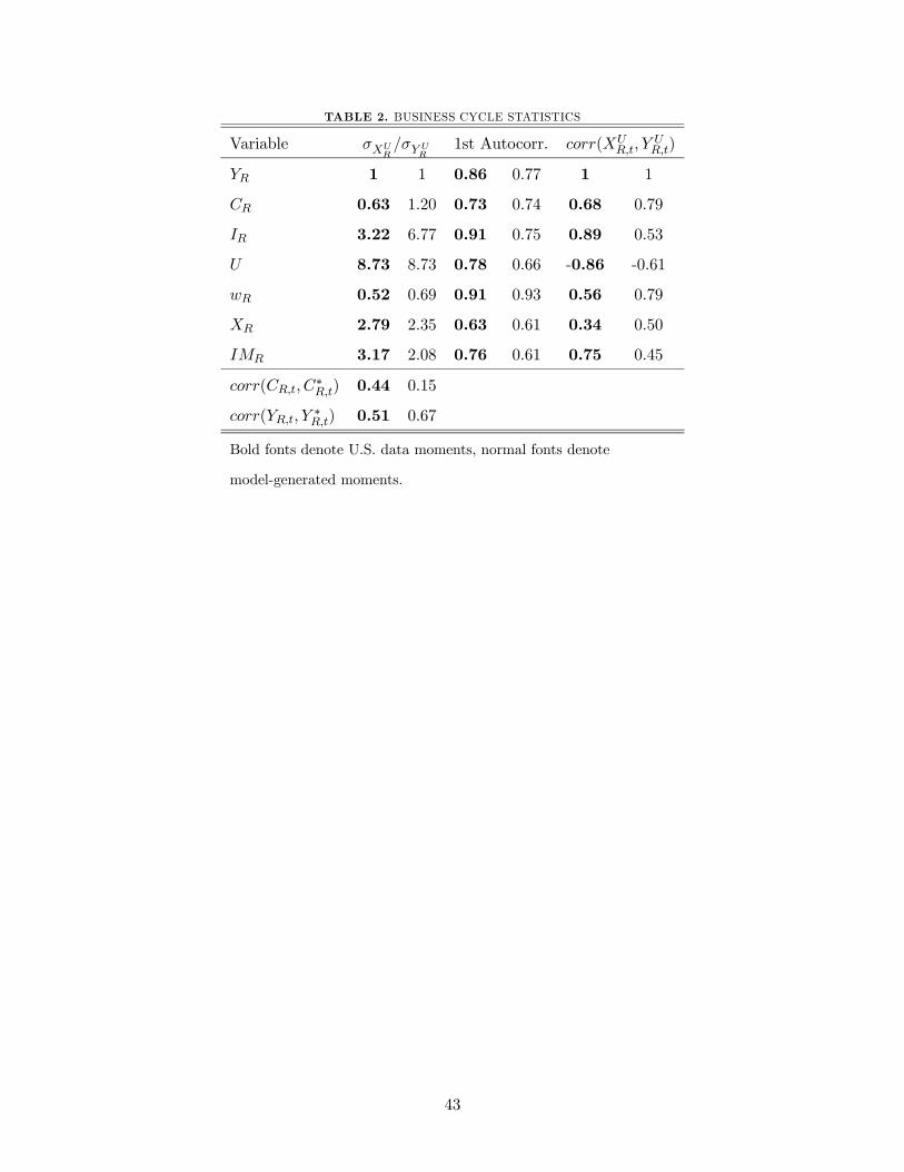
TABLE 2. BUSINESS CYCLE STATISTICS

Variable

1st Autocorr. (

)

1 1 0.86 0.77 1 1

0.63 1.20 0.73 0.74 0.68 0.79

3.22 6.77 0.91 0.75 0.89 0.53

8.73 8.73 0.78 0.66 -0.86 -0.61

0.52 0.69 0.91 0.93 0.56 0.79

2.79 2.35 0.63 0.61 0.34 0.50

3.17 2.08 0.76 0.61 0.75 0.45

( ∗) 0.44 0.15

( ∗) 0.51 0.67

Bold fonts denote U.S. data moments, normal fonts denote

model-generated moments.

43

TABLE 3. WELFARE EFFECTS OF REFORMS, NON STOCHASTIC STEADY STATE

Market Reform ∆Welfare (Historical) ∆Welfare (Ramsey) Ramsey Inflation

Home Foreign Home Foreign Home Foreign

Status Quo(Flexible Foreign)

0% 0% 0.54% 0.27% 1.85% 1.38%

PMR 2.34% 0.04% 2.84% 0.31% 1.81% 1.37%

LMR 3.93% 0.17% 4.23% 0.43% 1.40% 1.36%

JOINT 6.10% 0.21% 6.37% 0.46% 1.36% 1.36%

Note: PMR ≡ Product Market Reform; LMR ≡ Labor Market Reform;

JOINT ≡ Product and Labor Market Reform;

∆Welfare (Historical) ≡ Welfare change under historical policy;

∆Welfare (Ramsey) ≡ Welfare change under Ramsey policy.

44

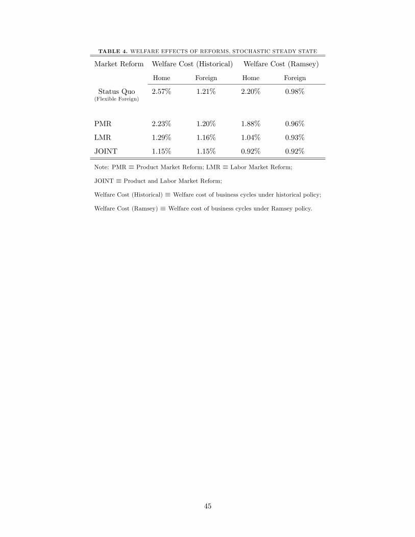
TABLE 4. WELFARE EFFECTS OF REFORMS, STOCHASTIC STEADY STATE

Market Reform Welfare Cost (Historical) Welfare Cost (Ramsey)

Home Foreign Home Foreign

Status Quo(Flexible Foreign)

2.57% 1.21% 2.20% 0.98%

PMR 2.23% 1.20% 1.88% 0.96%

LMR 1.29% 1.16% 1.04% 0.93%

JOINT 1.15% 1.15% 0.92% 0.92%

Note: PMR ≡ Product Market Reform; LMR ≡ Labor Market Reform;

JOINT ≡ Product and Labor Market Reform;

Welfare Cost (Historical) ≡ Welfare cost of business cycles under historical policy;

Welfare Cost (Ramsey) ≡ Welfare cost of business cycles under Ramsey policy.

45

TABLE A.1. MODEL SUMMARY

1 = 1−

1−1− + ∗

1− ∗

1−1−

(1)

1 = ∗1−

1−1− +

1−

1−1− (2)

−−1− ∗

=(−1)

−(−1)

(3)

∗−

∗ −1−

=

(−1)−(−1)

∗∗

∗ (4)

=

+

++

(5)

∗∗ = ∗

∗

∗ +∗

∗

∗ +∗

∗∗+∗

∗∗

(6)

= (1− )−1+−1−1 (7)

∗= (1− )∗−1+∗−1

∗−1 (8)

1 =

⎧⎨⎩+1+1

⎡⎣ +1

³+1− +1

+1

+1

´+

1(−1)

³+1

+1 ++1

+1

+1+1+1

+1

+1+1

+1

´⎤⎦⎫⎬⎭ (9)

1 =

⎧⎪⎨⎪⎩∗+1

∗+1∗

⎡⎢⎣ ∗

∗+1

³∗+1∗− ∗+1

∗+1

∗+1∗

´+

1(−1)∗

³∗

∗+1

∗+1 +∗+1∗+1

∗+1∗+1

+1∗+1

∗+1

∗+1∗+1

´⎤⎥⎦⎫⎪⎬⎪⎭ (10)

1 =

n+1

h(1− )

+1+

³+1+1+1 − +1

+1+1 −

22+1

´io(11)

1 =

n∗+1

h(1− )

∗∗+1

+∗

³∗+1

∗+1

∗+1 −

∗+1∗+1

∗+1 − 2∗2+1

´io(12)

= (13)

∗∗ = ∗∗ (14)

=−1

(15)

∗ =∗∗−1

∗ (16)

=

³()

+ ´+ (1− )

¡ −

22

¢+

n+1+1

h(1− )(1− )− (1− − )(1− +1)

+1

io (17)

∗∗

∗ = ∗³(∗ )∗

+ ∗´+ (1− ∗ )

¡∗∗ ∗ −

2∗2

¢+

n∗+1∗+1

h(1− )(1− ∗ )− (1− − ∗ )(1− ∗+1)

∗∗+1

io (18)

1 + +1 = (1 + )h(1 + ) (1 + )

³

´ i1−(19)

1 + ∗+1 = (1 + ∗ )h(1 + ∗)

³1 + ∗

´ ³ ∗

´ i1−(20)

1++1 = (1++1)+1

³1

1++1

´(21)

1− ∗∗+1 =¡1 + ∗+1

¢+1

³+1

11+∗

+1

´(22)

1+∗∗+1 =¡1+∗+1

¢

∗+1

³1

1+∗+1

´(23)

1− +1 = (1 + +1)∗+1

³

+1

11++1

´(24)

+1 =1+1+

−1+∗1+∗

∗∗ + −∗

∗

∗ (25)

46

TABLE A.2. LONG-RUN AVERAGE PRODUCTIVITY

Market Reform ∆ Average Productivity (Historical) ∆ Average Productivity (Ramsey)

Home Foreign Home Foreign

Status Quo(Flexible Foreign)

0% 0% 0% 0%

PMR 0.35% -0.03% 0.37% -0.03%

LMR 0.11% -0.10% 0.11% -0.10%

JOINT 0.46% -0.13% 0.46% -0.13%

Note: PMR ≡ Product Market Reform; LMR ≡ Labor Market Reform;

JOINT ≡ Product and Labor Market Reform;

∆ Average Productivity (Historical) ≡ Average productivity change under historical policy;

∆ Average Productivity (Ramsey) ≡ Average productivity change under Ramsey policy;

47

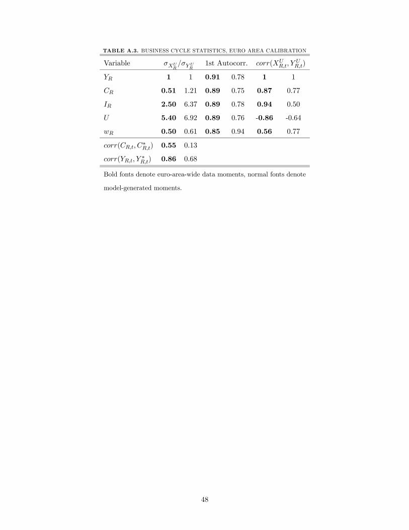
TABLE A.3. BUSINESS CYCLE STATISTICS, EURO AREA CALIBRATION

Variable

1st Autocorr. (

)

1 1 0.91 0.78 1 1

0.51 1.21 0.89 0.75 0.87 0.77

2.50 6.37 0.89 0.78 0.94 0.50

5.40 6.92 0.89 0.76 -0.86 -0.64

0.50 0.61 0.85 0.94 0.56 0.77

( ∗) 0.55 0.13

( ∗) 0.86 0.68

Bold fonts denote euro-area-wide data moments, normal fonts denote

model-generated moments.

48

TABLE A.4. WELFARE EFFECTS OF REFORMS, NON STOCHASTIC STEADY STATE, EURO AREA CALIBRATION

Market Reform ∆Welfare (Historical) ∆Welfare (Ramsey) Ramsey Inflation

Home Foreign Home Foreign Home Foreign

Status Quo(Rigid Foreign)

0% 0% 0.57% 0.57% 1.87% 1.87%

Asymmetric PMR 2.57% 0.05% 3.10% 0.62% 1.82% 1.87%

Asymmetric LMR 4.20% 0.22% 4.51% 0.77% 1.39% 1.86%

Asymmetric JOINT 6.14% 0.24% 6.44% 0.79% 1.38% 1.85%

Symmetric PMR 2.62% 2.62% 3.15% 3.15% 1.82% 1.82%

Symmetric LMR 4.39% 4.39% 4.67% 4.67% 1.38% 1.38%

Symmetric JOINT 6.33% 6.33% 6.60% 6.60% 1.37% 1.37%

Note: PMR ≡ Product Market Reform; LMR ≡ Labor Market Reform;

JOINT ≡ Product and Labor Market Reform; Asymmetric ≡ Home country reform;

Symmetric ≡ Home and Foreign country reform;

∆Welfare (Historical) ≡ Welfare change under historical policy;

∆Welfare (Ramsey) ≡ Welfare change under Ramsey policy.

49

TABLE A.5. WELFARE EFFECTS OF REFORMS, STOCHASTIC STEADY STATE, EURO AREA CALIBRATION

Market Reform Welfare Cost (Historical) Welfare Cost (Ramsey)

Home Foreign Home Foreign

Status Quo(Rigid Foreign)

2.68% 2.68% 2.29% 2.29%

Asymmetric PMR 2.29% 2.65% 1.94% 2.26%

Asymmetric LMR 1.23% 2.58% 0.99% 2.20%

Asymmetric JOINT 1.21% 2.57% 0.98% 2.19%

Symmetric PMR 2.26% 2.26% 1.92% 1.92%

Symmetric LMR 1.17% 1.17% 0.94% 0.94%

Symmetric JOINT 1.16% 1.16% 0.93% 0.93%

Note: PMR ≡ Product Market Reform; LMR ≡ Labor Market Reform;

JOINT ≡ Product and Labor Market Reform; Asymmetric ≡ Home country reform;

Symmetric ≡ Home and Foreign country reform;

Welfare Cost (Historical) ≡ Welfare cost of business cycles under historical policy;

Welfare Cost (Ramsey) ≡ Welfare cost of business cycles under Ramsey policy.

50

TABLE A.6. LONG-RUN AVERAGE PRODUCTIVITY, EURO AREA CALIBRATION

Market Reform ∆ Average Productivity (Historical) ∆ Average Productivity (Ramsey)

Home Foreign Home Foreign

Status Quo(Rigid Foreign)

0% 0% 0% 0%

Asymmetric PMR 0.38% -0.03% 0.38% -0.03%

Asymmetric LMR 0.12% -0.12% 0.11% -0.11%

Asymmetric JOINT 0.44% -0.14% 0.44% -0.13%

Symmetric PMR 0.35% 0.35% 0.35% 0.35%

Symmetric LMR 0.00% 0.00% 0.00% 0.00%

Symmetric JOINT 0.32% 0.32% 0.32% 0.32%

Note: PMR ≡ Product Market Reform; LMR ≡ Labor Market Reform;

JOINT ≡ Product and Labor Market Reform; Asymmetric ≡ Home country reform;

Symmetric ≡ Home and Foreign country reform;

∆ Average Productivity (Historical) ≡ Average productivity change under historical policy;

∆ Average Productivity (Ramsey) ≡ Average productivity change under Ramsey policy;

51

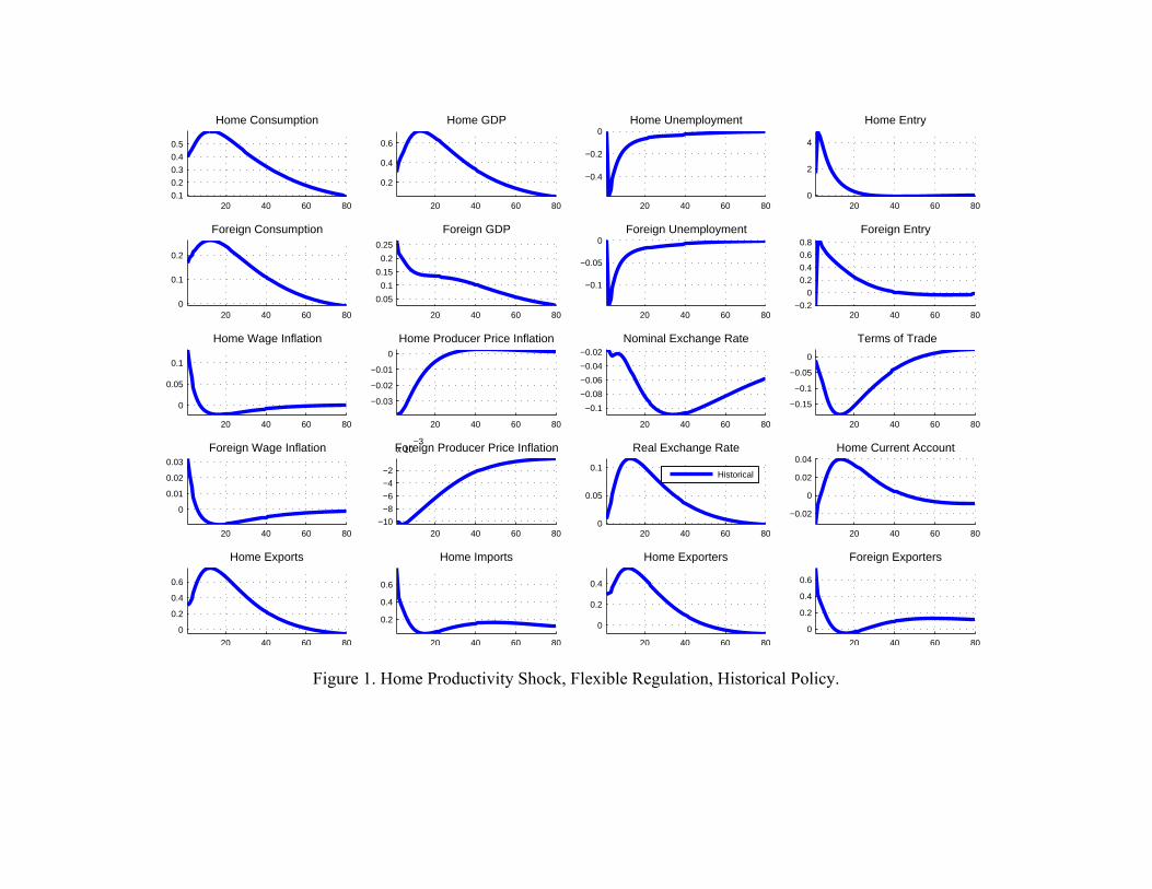
Figure 1. Home Productivity Shock, Flexible Regulation, Historical Policy.

20 40 60 800.1

0.2

0.3

0.4

0.5

Home Consumption

20 40 60 80

0.2

0.4

0.6

Home GDP

20 40 60 80

−0.4

−0.2

0Home Unemployment

20 40 60 800

2

4

Home Entry

20 40 60 800

0.1

0.2

Foreign Consumption

20 40 60 80

0.05

0.1

0.15

0.2

0.25

Foreign GDP

20 40 60 80

−0.1

−0.05

0Foreign Unemployment

20 40 60 80−0.2

00.20.40.60.8

Foreign Entry

20 40 60 80

0

0.05

0.1

Home Wage Inflation

20 40 60 80

−0.03

−0.02

−0.01

0

Home Producer Price Inflation

20 40 60 80

−0.1

−0.08

−0.06

−0.04

−0.02

Nominal Exchange Rate

20 40 60 80

−0.15

−0.1

−0.05

0

Terms of Trade

20 40 60 80

0

0.01

0.02

0.03

Foreign Wage Inflation

20 40 60 80−10

−8

−6

−4

−2

x 10−3

Foreign Producer Price Inflation

20 40 60 800

0.05

0.1

Real Exchange Rate

Historical

20 40 60 80

−0.02

0

0.02

0.04Home Current Account

20 40 60 80

0

0.2

0.4

0.6

Home Exports

20 40 60 80

0.2

0.4

0.6

Home Imports

20 40 60 80

0

0.2

0.4

Home Exporters

20 40 60 80

0

0.2

0.4

0.6

Foreign Exporters

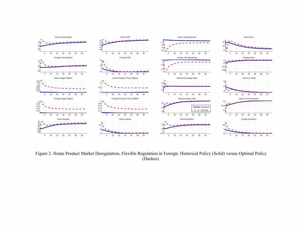
Figure 2. Home Product Market Deregulation, Flexible Regulation in Foreign. Historical Policy (Solid) versus Optimal Policy (Dashes).

5 10 15 20 25 30 35

−2

0

2

Home Consumption

5 10 15 20 25 30 35

−6−4−2

02

Home GDP

5 10 15 20 25 30 35

−4−3−2−1

Home Unemployment

5 10 15 20 25 30 35

5

10

15

Home Entry

5 10 15 20 25 30 35

−2

0

2

Foreign Consumption

5 10 15 20 25 30 350

2

4Foreign GDP

5 10 15 20 25 30 35

−2

−1

0Foreign Unemployment

5 10 15 20 25 30 35

−15

−10

−5

0

Foreign Entry

5 10 15 20 25 30 35

0.20.40.60.8

11.21.4

Home Wage Inflation

5 10 15 20 25 30 350

0.5

1

Home Producer Price Inflation

5 10 15 20 25 30 35

−2

0

2

Nominal Exchange Rate

5 10 15 20 25 30 35

0

2

4

Terms of Trade

5 10 15 20 25 30 35

0.20.40.60.8

1

Foreign Wage Inflation

5 10 15 20 25 30 35

0.20.40.60.8

1Foreign Producer Price Inflation

5 10 15 20 25 30 35

−2

−1

0

Real Exchange Rate

Historical

Ramsey

5 10 15 20 25 30 35

−1

−0.5

0Home Current Account

5 10 15 20 25 30 35

−8−6−4−2

024

Home Exports

5 10 15 20 25 30 350

5

10

Home Imports

5 10 15 20 25 30 35−10

−5

0

Home Exporters

5 10 15 20 25 30 350

5

10

Foreign Exporters

Figure 2b. Home Product Market Deregulation, Productivity and Labor Reallocation Effects.

5 10 15 20 25 30 35

0

0.2

0.4

Average Productivity, Home

5 10 15 20 25 30 35−1

−0.5

0

0.5

1Average Productivity, Domestic Sales, Home

5 10 15 20 25 30 35

0

1

2

3

Average Productivity, Export Sales, Home

5 10 15 20 25 30 35

−0.2

0

0.2

Average Employment, Home

5 10 15 20 25 30 35−0.2

0

0.2

Average Employment, Domestic Sales, Home

5 10 15 20 25 30 35−1

−0.5

0

0.5

1Average Employment, Export Sales, Home

5 10 15 20 25 30 35

−0.6

−0.4

−0.2

Average Productivity, Foreign

5 10 15 20 25 30 35−1

−0.5

0

0.5

1Average Productivity, Domestic Sales, Foreign

5 10 15 20 25 30 35

−3

−2

−1

Average Productivity, Export Sales, Foreign

5 10 15 20 25 30 35

0.1

0.2

0.3

Average Employment, Foreign

5 10 15 20 25 30 35

0.05

0.1

0.15

0.2

0.25

Average Employment, Domestic Sales, Foreign

5 10 15 20 25 30 35−1

−0.5

0

0.5

1Average Employment, Export Sales, Foreign

HistoricalRamsey

Figure 3. Home Labor Market Deregulation, Flexible Regulation in Foreign. Historical Policy (Solid) versus Optimal Policy (Dashes).

5 10 15 20 25 30 35

2

4

6Home Consumption

5 10 15 20 25 30 350

2

4

Home GDP

5 10 15 20 25 30 35

−6

−4

−2

Home Unemployment

5 10 15 20 25 30 35

−20

−10

0

Home Entry

5 10 15 20 25 30 35

0

1

2

Foreign Consumption

5 10 15 20 25 30 350

1

2

Foreign GDP

5 10 15 20 25 30 35

−2

−1

0Foreign Unemployment

5 10 15 20 25 30 35

−10

−5

0

Foreign Entry

5 10 15 20 25 30 35

0

0.5

1

Home Wage Inflation

5 10 15 20 25 30 350

0.5

1

Home Producer Price Inflation

5 10 15 20 25 30 35−0.5

0

0.5

1

Nominal Exchange Rate

5 10 15 20 25 30 35

−0.5

0

0.5

Terms of Trade

5 10 15 20 25 30 35

0.20.40.60.8

1

Foreign Wage Inflation

5 10 15 20 25 30 35

0.20.40.60.8

1Foreign Producer Price Inflation

5 10 15 20 25 30 35

−0.20

0.20.40.6

Real Exchange Rate

Historical

Ramsey

5 10 15 20 25 30 35

−0.4

−0.2

0

Home Current Account

5 10 15 20 25 30 35

0246

Home Exports

5 10 15 20 25 30 352468

10

Home Imports

5 10 15 20 25 30 35

0246

Home Exporters

5 10 15 20 25 30 352

4

6

8

10Foreign Exporters

Figure 3b. Home Labor Market Deregulation, Productivity and Labor Reallocation Effects.

5 10 15 20 25 30 35−0.4

−0.2

0

Average Productivity, Home

5 10 15 20 25 30 35−1

−0.5

0

0.5

1Average Productivity, Domestic Sales, Home

5 10 15 20 25 30 35

−2

−1

0

Average Productivity, Export Sales, Home

5 10 15 20 25 30 35

0.1

0.2

0.3

0.4

0.5

Average Employment, Home

5 10 15 20 25 30 35

0.1

0.2

0.3

0.4

0.5Average Employment, Domestic Sales, Home

5 10 15 20 25 30 35−1

−0.5

0

0.5

1Average Employment, Export Sales, Home

5 10 15 20 25 30 35−0.5

−0.4

−0.3

−0.2

−0.1Average Productivity, Foreign

5 10 15 20 25 30 35−1

−0.5

0

0.5

1Average Productivity, Domestic Sales, Foreign

5 10 15 20 25 30 35

−2.5

−2

−1.5

−1

Average Productivity, Export Sales, Foreign

5 10 15 20 25 30 350

0.1

0.2

Average Employment, Foreign

5 10 15 20 25 30 350

0.05

0.1

0.15

0.2

Average Employment, Domestic Sales, Foreign

5 10 15 20 25 30 35−1

−0.5

0

0.5

1Average Employment, Export Sales, Foreign

HistoricalRamsey

Figure 4. Home Product and Labor Market Deregulation, Flexible Regulation in Foreign. Historical Policy (Solid) versus Optimal Policy (Dashes).

5 10 15 20 25 30 35

2

4

6

Home Consumption

5 10 15 20 25 30 35

0

2

4

6

Home GDP

5 10 15 20 25 30 35

−6

−4

−2

Home Unemployment

5 10 15 20 25 30 35

−100

1020

Home Entry

5 10 15 20 25 30 35

−2

0

2

Foreign Consumption

5 10 15 20 25 30 35

−2

0

2

4

Foreign GDP

5 10 15 20 25 30 35−4

−2

0Foreign Unemployment

5 10 15 20 25 30 35

−10

−5

0

Foreign Entry

5 10 15 20 25 30 350

0.5

1

Home Wage Inflation

5 10 15 20 25 30 350

0.5

1

Home Producer Price Inflation

5 10 15 20 25 30 35−2

−1

0

Nominal Exchange Rate

5 10 15 20 25 30 35−1

0

1

2

Terms of Trade

5 10 15 20 25 30 35

0.20.40.60.8

11.21.4

Foreign Wage Inflation

5 10 15 20 25 30 350

0.5

1

Foreign Producer Price Inflation

5 10 15 20 25 30 35

−1

0

1

Real Exchange Rate

Historical

Ramsey

5 10 15 20 25 30 35

−0.8−0.6−0.4−0.2

0

Home Current Account

5 10 15 20 25 30 35

−5

0

5Home Exports

5 10 15 20 25 30 352468

101214

Home Imports

5 10 15 20 25 30 35−6−4−2

02

Home Exporters

5 10 15 20 25 30 352468

101214

Foreign Exporters

Figure 4b. Home Product and Labor Market Deregulation, Productivity and Labor Reallocation Effects.

5 10 15 20 25 30 35

−0.1

0

0.1

0.2

0.3

Average Productivity, Home

5 10 15 20 25 30 35−1

−0.5

0

0.5

1Average Productivity, Domestic Sales, Home

5 10 15 20 25 30 35

0

1

2

Average Productivity, Export Sales, Home

5 10 15 20 25 30 35−0.2

0

0.2

0.4Average Employment, Home

5 10 15 20 25 30 35−0.2

0

0.2

0.4Average Employment, Domestic Sales, Home

5 10 15 20 25 30 35−1

−0.5

0

0.5

1Average Employment, Export Sales, Home

HistoricalRamsey

5 10 15 20 25 30 35

−0.6

−0.4

−0.2

Average Productivity, Foreign

5 10 15 20 25 30 35−1

−0.5

0

0.5

1Average Productivity, Domestic Sales, Foreign

5 10 15 20 25 30 35−4

−3

−2

−1

Average Productivity, Export Sales, Foreign

5 10 15 20 25 30 350

0.1

0.2

Average Employment, Foreign

5 10 15 20 25 30 350

0.05

0.1

0.15

0.2

Average Employment, Domestic Sales, Foreign

5 10 15 20 25 30 35−1

−0.5

0

0.5

1Average Employment, Export Sales, Foreign

HistoricalRamsey

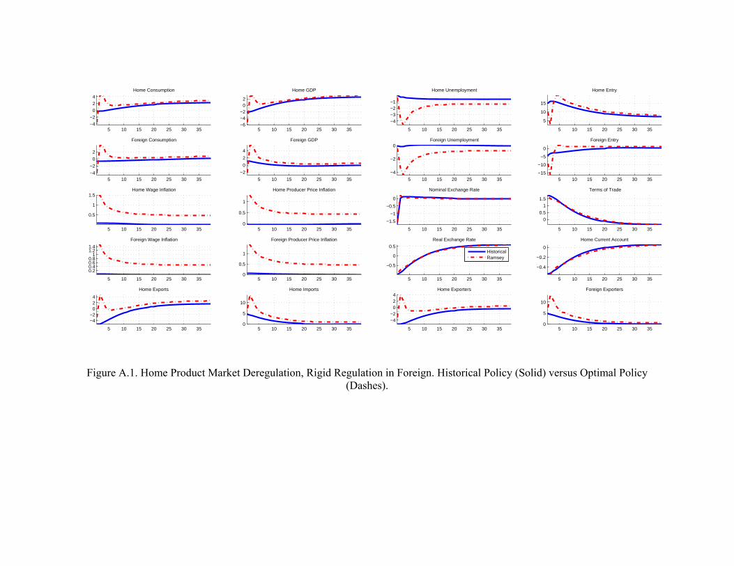
Figure A.1. Home Product Market Deregulation, Rigid Regulation in Foreign. Historical Policy (Solid) versus Optimal Policy (Dashes).

5 10 15 20 25 30 35−4

−2

0

2

4Home Consumption

5 10 15 20 25 30 35−6−4−2

02

Home GDP

5 10 15 20 25 30 35

−4−3−2−1

Home Unemployment

5 10 15 20 25 30 35

5

10

15

Home Entry

5 10 15 20 25 30 35−4

−2

0

2

Foreign Consumption

5 10 15 20 25 30 35

−2

0

2

4

Foreign GDP

5 10 15 20 25 30 35

−4

−2

0Foreign Unemployment

5 10 15 20 25 30 35−15

−10

−5

0

Foreign Entry

5 10 15 20 25 30 35

0.5

1

1.5Home Wage Inflation

5 10 15 20 25 30 350

0.5

1

Home Producer Price Inflation

5 10 15 20 25 30 35

−1.5

−1

−0.5

0

Nominal Exchange Rate

5 10 15 20 25 30 35

0

0.5

1

1.5

Terms of Trade

5 10 15 20 25 30 35

0.20.40.60.8

11.21.4

Foreign Wage Inflation

5 10 15 20 25 30 350

0.5

1

Foreign Producer Price Inflation

5 10 15 20 25 30 35

−0.5

0

0.5

Real Exchange Rate

HistoricalRamsey

5 10 15 20 25 30 35

−0.4

−0.2

0

Home Current Account

5 10 15 20 25 30 35

−4−2

024

Home Exports

5 10 15 20 25 30 350

5

10

Home Imports

5 10 15 20 25 30 35

−4−2

024

Home Exporters

5 10 15 20 25 30 350

5

10

Foreign Exporters

Figure A.2. Home Labor Market Deregulation, Rigid Regulation in Foreign. Historical Policy (Solid) versus Optimal Policy (Dashes).

5 10 15 20 25 30 35

2

4

6

Home Consumption

5 10 15 20 25 30 35

2

4

6

Home GDP

5 10 15 20 25 30 35

−6

−4

−2

Home Unemployment

5 10 15 20 25 30 35

−30−20−10

010

Home Entry

5 10 15 20 25 30 35

−2

0

2

4Foreign Consumption

5 10 15 20 25 30 35

−2024

Foreign GDP

5 10 15 20 25 30 35−4

−2

0Foreign Unemployment

5 10 15 20 25 30 35−10

−5

0

Foreign Entry

5 10 15 20 25 30 35

0

0.5

1

Home Wage Inflation

5 10 15 20 25 30 350

0.5

1

Home Producer Price Inflation

5 10 15 20 25 30 35

−2

0

2Nominal Exchange Rate

5 10 15 20 25 30 35−2

−1

0

1Terms of Trade

5 10 15 20 25 30 350

0.5

1

Foreign Wage Inflation

5 10 15 20 25 30 35

0.20.40.60.8

11.2

Foreign Producer Price Inflation

5 10 15 20 25 30 35−0.5

0

0.5

1

Real Exchange Rate

Historical

Ramsey

5 10 15 20 25 30 35

−0.4

−0.2

0

0.2

Home Current Account

5 10 15 20 25 30 35−2

02468

Home Exports

5 10 15 20 25 30 352468

10

Home Imports

5 10 15 20 25 30 35−2

02468

Home Exporters

5 10 15 20 25 30 352468

10

Foreign Exporters

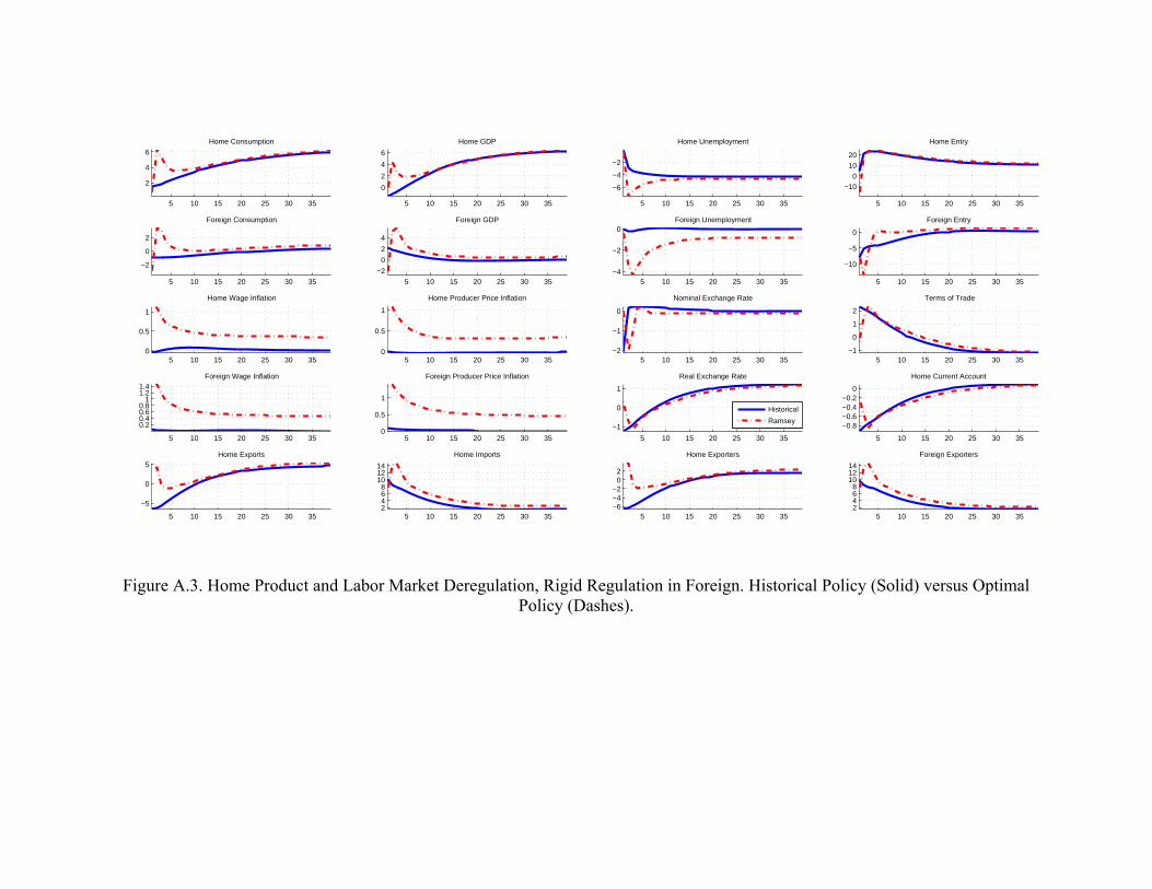
Figure A.3. Home Product and Labor Market Deregulation, Rigid Regulation in Foreign. Historical Policy (Solid) versus Optimal Policy (Dashes).

5 10 15 20 25 30 35

2

4

6

Home Consumption

5 10 15 20 25 30 35

0

2

4

6

Home GDP

5 10 15 20 25 30 35

−6

−4

−2

Home Unemployment

5 10 15 20 25 30 35

−100

1020

Home Entry

5 10 15 20 25 30 35

−2

0

2

Foreign Consumption

5 10 15 20 25 30 35

−2

0

2

4

Foreign GDP

5 10 15 20 25 30 35−4

−2

0Foreign Unemployment

5 10 15 20 25 30 35

−10

−5

0

Foreign Entry

5 10 15 20 25 30 350

0.5

1

Home Wage Inflation

5 10 15 20 25 30 350

0.5

1

Home Producer Price Inflation

5 10 15 20 25 30 35−2

−1

0

Nominal Exchange Rate

5 10 15 20 25 30 35−1

0

1

2

Terms of Trade

5 10 15 20 25 30 35

0.20.40.60.8

11.21.4

Foreign Wage Inflation

5 10 15 20 25 30 350

0.5

1

Foreign Producer Price Inflation

5 10 15 20 25 30 35

−1

0

1

Real Exchange Rate

Historical

Ramsey

5 10 15 20 25 30 35

−0.8−0.6−0.4−0.2

0

Home Current Account

5 10 15 20 25 30 35

−5

0

5Home Exports

5 10 15 20 25 30 352468

101214

Home Imports

5 10 15 20 25 30 35−6−4−2

02

Home Exporters

5 10 15 20 25 30 352468

101214

Foreign Exporters