
TheBookOfSho
77
The Book of Sho by the Team of Sho
-
Upload
laraleopoldo -
Category
Documents
-
view
325 -
download
3
Transcript of TheBookOfSho

The Book of Sho
by the Team of Sho

2
3
Table of Contents
Chapter 1: What Is Sho? ........................................................................................................................... 5 1.1 Welcome to Sho .............................................................................................................................. 5 1.2 What Sho Is .................................................................................................................................... 5
1.2.1 What Sho Looks Like ............................................................................................................... 5 1.2.2 How Sho Relates to IronPython and .NET................................................................................. 5
1.3 Why Should I Use Sho? .................................................................................................................. 6 Chapter 2: Getting Started ......................................................................................................................... 7
2.1 The Sho Environment...................................................................................................................... 7 2.1.1 The Sho Console ...................................................................................................................... 7 2.1.2 Editing Python Files, Functions, and Modules ........................................................................... 8 2.1.3 Browsing the Command History ............................................................................................... 9 2.1.4 Using Sho from the Command Shell ......................................................................................... 9
2.2 OS Utilities ................................................................................................................................... 10 2.3 Odds and Ends .............................................................................................................................. 11 2.4 Documentation Utilities ................................................................................................................ 11
2.4.1 The help function ................................................................................................................... 11 2.4.2 Using doc to Examine Types or Objects .................................................................................. 11 2.4.3 The lookup utility ................................................................................................................... 13
Chapter 3: IronPython Basics .................................................................................................................. 15 3.1 Python vs. IronPython ................................................................................................................... 15 3.2 Types ............................................................................................................................................ 15 3.3 Formatting Code ........................................................................................................................... 16 3.4 Conditionals .................................................................................................................................. 16 3.5 Built-in Collections: Lists, Tuples and Dictionaries........................................................................ 16 3.6 Loops and Iterators........................................................................................................................ 18 3.7 Manipulating Lists ........................................................................................................................ 19
3.7.1 List Comprehensions .............................................................................................................. 19 3.7.2 List ........................................................................................................................................ 19 3.7.3 Zip ......................................................................................................................................... 20 3.7.4 Sort ........................................................................................................................................ 20
3.8 Dictionaries and Hashtables .......................................................................................................... 20 3.9 Using .NET Generics .................................................................................................................... 21 3.10 Functions .................................................................................................................................... 21
3.10.1 Default Values and Named Arguments .................................................................................. 22 3.10.2 Function Pointers and Delegates ........................................................................................... 22 3.10.3 Yield .................................................................................................................................... 22
3.11 Classes ........................................................................................................................................ 23 3.12 Files and Namespaces ................................................................................................................. 24
3.12.1 Execfile ................................................................................................................................ 24 3.12.2 Import .................................................................................................................................. 25 3.12.3 From <module> import <symbol> ........................................................................................ 26
3.13 Exceptions .................................................................................................................................. 26 3.14 ShoThreads ................................................................................................................................. 27
Chapter 4: Matrix Classes ....................................................................................................................... 29 4.1 Array Creation .............................................................................................................................. 29 4.2 Element Access and Slicing........................................................................................................... 31 4.3 Optimized Matrix Methods............................................................................................................ 32 4.4 Sparse Arrays ................................................................................................................................ 33 4.5 Multidimensional Arrays ............................................................................................................... 34 4.6 Group and Elementwise Operations ............................................................................................... 35 4.7 The Find Command ...................................................................................................................... 36 4.8 Linear Algebra .............................................................................................................................. 37
Chapter 5: Math and Data Analysis ......................................................................................................... 39

4
5.1 Mapping functions ........................................................................................................................ 39 5.2 Stepping through intervals ............................................................................................................. 39 5.3 Histogramming ............................................................................................................................. 40
Chapter 6: Data Handling ....................................................................................................................... 42 6.1 Pickling Sho data .......................................................................................................................... 42 6.2 Reading/Writing Delimited Files ................................................................................................... 42 6.3 Reading from a Database............................................................................................................... 43 6.4 Roll your own data readers/writers ................................................................................................ 44
6.4.1 Custom ASCII Data Reader .................................................................................................... 44 6.4.2 Custom Binary Data Reader.................................................................................................... 44
Chapter 7: Plotting and visualization ....................................................................................................... 46 7.1 Line/scatter plots ........................................................................................................................... 46
7.1.1 Multiple Plots ......................................................................................................................... 49 7.1.2 Advanced Plot Options ........................................................................................................... 50 7.1.3 Legends.................................................................................................................................. 51 7.1.4 Drawing Images, Lines, Shapes, and Text onto Plots ............................................................... 52 7.1.5 Setting Plot Properties ............................................................................................................ 53
7.2 Bar Charts ..................................................................................................................................... 54 7.3 DataGridView ............................................................................................................................... 56 7.4 Contour Plots ................................................................................................................................ 58 7.5 Viewing Arrays as Images ............................................................................................................. 58 7.6 Interactive Histograms .................................................................................................................. 60 7.7 Inline plots in ShoConsole ............................................................................................................. 60 7.8 Copying, Exporting, and Saving Plots............................................................................................ 61
Chapter 8: .NET ..................................................................................................................................... 62 8.1 Using .NET Framework Classes .................................................................................................... 62 8.2 Using Other .NET Libraries .......................................................................................................... 62 8.3 Using COM Libraries .................................................................................................................... 63
Chapter 9: Extending Sho ....................................................................................................................... 64 9.1 Python Modules ............................................................................................................................ 64 9.2 Single C# Files .............................................................................................................................. 64 9.3 Dynamically Extending Sho with Visual Studio ............................................................................. 66
9.3.1 Signing the Assembly ............................................................................................................. 66 9.3.2 Auto-Updating the Assembly Version ..................................................................................... 67 9.3.3 Loading/Reloading the Assembly from Sho ............................................................................ 67 9.3.4 Debugging the Assembly ........................................................................................................ 68
9.4 Sho Packages ................................................................................................................................ 68 Chapter 10: Using Sho from .NET .......................................................................................................... 70
10.1 Writing .NET Code Using Sho Libraries ...................................................................................... 70 10.2 Calling Python Code from .NET .................................................................................................. 71
Chapter 11: Writing GUIs with Sho ........................................................................................................ 73 Chapter 12: Debugging Sho Code ........................................................................................................... 75
12.1 Debugging Sho Code from Sho ................................................................................................... 75 12.2 Debugging with Visual Studio ..................................................................................................... 75
Chapter 13: Epilogue .............................................................................................................................. 77 13.1 Other Resources .......................................................................................................................... 77 13.2 And You‟re Off! ......................................................................................................................... 77
5
Chapter 1: What Is Sho?
1.1 Welcome to Sho
Hello, and welcome to Sho. If you‟ve come this far, you‟ve most likely heard something about Sho and
want to find out more, and hopefully this guidebook will help you get started. The goal with this book is
not to give you a comprehensive command reference, but enough of a tour of the major features to let you
know what‟s available. If you find yourself at a point where you toss this book aside and just start hacking in Sho, we will have accomplished our purpose.
1.2 What Sho Is
Sho is an interactive environment for data input, analysis, and visualization, built on top of the IronPython
programming language. It has facilities for mathematical representations and operations, plotting data,
database access, and much more. It‟s command-line based, which means no fancy GUI with buttons and
panes and all the rest. You can build such GUIs from inside Sho, as we‟ll show later, but the basic interface
is just a prompt. The great thing is that you can define a matrix and look at its elements, open up a database and plot data from it, try various settings of your C# algorithm on a batch of data, all with just a few
interactively-typed lines at that simple prompt.
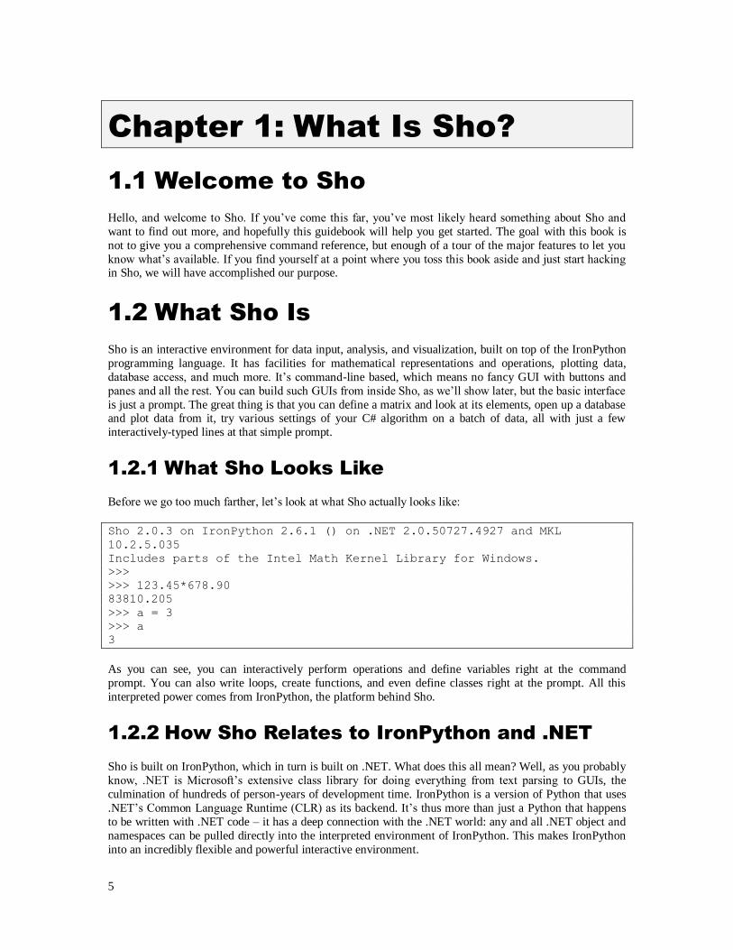
1.2.1 What Sho Looks Like
Before we go too much farther, let‟s look at what Sho actually looks like:
Sho 2.0.3 on IronPython 2.6.1 () on .NET 2.0.50727.4927 and MKL
10.2.5.035
Includes parts of the Intel Math Kernel Library for Windows.
>>>
>>> 123.45*678.90
83810.205
>>> a = 3
>>> a
3
As you can see, you can interactively perform operations and define variables right at the command
prompt. You can also write loops, create functions, and even define classes right at the prompt. All this
interpreted power comes from IronPython, the platform behind Sho.
1.2.2 How Sho Relates to IronPython and .NET
Sho is built on IronPython, which in turn is built on .NET. What does this all mean? Well, as you probably
know, .NET is Microsoft‟s extensive class library for doing everything from text parsing to GUIs, the
culmination of hundreds of person-years of development time. IronPython is a version of Python that uses
.NET‟s Common Language Runtime (CLR) as its backend. It‟s thus more than just a Python that happens
to be written with .NET code – it has a deep connection with the .NET world: any and all .NET object and
namespaces can be pulled directly into the interpreted environment of IronPython. This makes IronPython
into an incredibly flexible and powerful interactive environment.

6
So what does Sho add to the mix? Basically, we have added a number of class libraries, utilities, and
interfaces to extend the IronPython environment into an ideal playground for data analysis and
manipulation. This includes math, plotting, and visualization facilities, as well as a host of utilities that
make it easy and fun to do research and prototyping in a mixed-language environment.
1.3 Why Should I Use Sho?
Sho is a great environment for all kinds of research and rapid prototyping work. While of course it‟s not
always the right tool for the job, we think there are lots of good reasons to use it for your work:
Sho Lets You Play with Objects and Data Interactively. Once you‟re working in Sho, you can
manipulate arbitrary parameters, call methods, investigate properties, instantiate new variables,
and the like for any .NET object, namespace, or class. Why is this useful? Well, you might not
know exactly what your data looks like, what kind of things a given method might return, which
class is the right one for the job, etc. Because you can try out a new class by just typing a few lines, it feels like you‟re “playing.”
Sho Makes Simple Things Simple. If all you need is load in some data and plot it, put up an
image in a window, or find all the records in a database that contain the string “foo”, you can do it
with just a few lines of Sho that you can type in interactively. If you‟re tired of writing, compiling,
and debugging a whole program just to do simple things, Sho might be for you.
Sho Lends Itself to Writing Modular Code. Because Sho makes it easy to load in a little piece
of functionality and apply it to arbitrary data, it lends itself to writing such little pieces instead of
big, monolithic programs. For instance, if you‟re writing a program that monitors web usage, you
might need a function that pulls out the domain name from a URL. Instead of burying this deep
inside a complex program, in Sho it‟s much more natural to just expose the function at the top
level. What‟s the advantage? This lets you test it easily, just by typing
GetDomainFromURL("http://www.mydomain.com/foo/bar.aspx") at the prompt.
Sho Is a Great Way to Share and Reuse Code. If you‟ve ever tried to use code from other
groups or colleagues, you know how much effort it can be just to get things compiled and working
together. Many people use their own math representations, incompatible libraries, threading
models, etc. Furthermore, it can be very difficult to figure out how to take code that‟s in a
monolithic program and extract out the functional pieces you‟re interested in. Sho helps with this in four ways. First, because it‟s all .NET, you can load in one assembly after another, and they will
all happily coexist in the same environment. Second, since everyone is writing against the same
Sho matrix, database, and other interfaces, the inputs and outputs of the functions will be naturally
compatible. Third, because Sho encourages modular code, it‟s much more likely that the libraries
will be full of individual functions instead of monolithic code paths. Finally, Sho makes it easy to
browse and play with the functions you pull in, so figuring out how to use the different libraries
together is much easier. This is particularly true since Sho/IronPython is dynamically typed, so
you can iterate through and print information from types that you know little or nothing about. In
addition, we have facilities like doc(obj) which use .NET reflection to investigate what‟s inside
a class or variable.

7
Chapter 2: Getting Started
2.1 The Sho Environment
Sho can be used in two ways: by running the Sho Console, which has a variety of fancy features like tab
completion, history recall, key bindings, etc., or directly within the command shell (cmd), which is limited
in its editing capabilities.
2.1.1 The Sho Console
Figure 2.1: The Sho Console showing tab completion.
The Sho Console is our recommended means of accessing Sho, and has many features, as we describe below. Here‟s a rundown of the principal features:
Tab Completion and Inline Documentation. Hit Tab after typing the partial name of a .NET or
Python class, method, namespace, or function, and the console will list all the possible
completions beneath the prompt. Hit Tab after typing a function/method name and an open
parenthesis or within the argument list, and the console will list all the prototypes for that function;
if there is documentation available it will show that as well.
Command History Recall. Type a few characters and hit up-arrow; the console will then retrieve
all commands you‟ve entered that started with those characters.
Rich Copy/Paste with C-c/v. This is the behavior you‟re used to in other windows applications,
as opposed to the command shell‟s non-standard behavior. However, Sho‟s rich copy and paste
also lets you paste in images, Excel ranges, and other data from sources outside Sho.
Break Execution with Ctrl-Alt-C or Ctrl-Shift-C. Use this to stop any foreground Sho task and
get back a command prompt.

8
Visual History Browser. You can bring up a history browser that persists across sessions by
typing “historypicker()”; this includes a search box at the top where you can do
incremental search on your past commands.
Inline graphics. You can view charts and graphs inline in the console window using the
showplot, showbar and show commands.
There‟s also an extensive set of key bindings (many of these will be familiar to Emacs users):
Ctrl-a: Beginning of Line
Ctrl-e: End of Line
Ctrl-b: Backwards Character
Ctrl-f: Forwards Character
Ctrl-p: Previous line in history (same as Up-Arrow)
Ctrl-n: Next line in history (same as Down-Arrow)
Ctrl-k: Clear to end-of-line
Alt-f: Forward word
Alt-b: Backward word
Ctrl-Alt-c: Break execution
Ctrl-Alt-s: Suspend (pause) execution
Ctrl-Alt-q: Resume execution
Additionally, there is a “shell-escape” mode that allows you to quickly execute DOS-shell commands from
the Sho console. Just start your command with a „%‟, and the rest of the line will be send to the shell.
If you‟d like to change the font used by the Sho console, just call the setfont function (just type
“setfont()” in the console window). It will present you with a font selection dialog where you can
choose the font to use. You can also set the title of the console window using the setconsoletitle()
command.
2.1.2 Editing Python Files, Functions, and
Modules
You‟ll often want to edit a file, function, or Python module of your own, or perhaps look up the source for
a Python function in sho. You can use the edit() command to do all of these things:
edit(module) – opens the Python file implementing the specified module
edit(function or method) – opens the Python file containing the function at the appropriate line
number*
edit(class) – opens the Python file at the first line of the constructor*
edit(“filename.py”) – opens filename.py if it‟s in your sys.path; you can also specify the full
pathname
*The default editor is notepad.exe, since everybody has it; unfortunately, it does not have the ability to
jump to a specified line number. You can change the default editor by setting the sys.Sho.Editor
variable, and you can use the sys.Sho.EditorArgs to specify how to open the file at the appropriate
line number. For instance, if you want to use Visual Studio (devenv.exe) as your editor and have it open
files at the right number, you can do the following:
>>> sys.Sho.Editor = "devenv.exe" #note devenv.exe must be in your PATH
>>> sys.Sho.EditorArgs = "%f /command \"edit.goto %l\""
If you‟re an Emacs user, use the following commands:

9
>>> sys.Sho.Editor = "emacs.exe" #note emacs.exe must be in your PATH
>>> sys.Sho.EditorArgs = "+%l %f"
Note you can put these lines into your startup file (startup.py), which is in the root of your {SHODIR}.
2.1.3 Browsing the Command History
Sho 2.0 has added some commands to help you browse the Sho commands you‟ve typed in the past, both in the current session and in previous sessions:
history() will return a list of strings containing all the commands you‟ve entered in the current
session.
historypicker() will bring up the GUI in the figure below, containing the last month of
history from all Sho sessions; you can specify the number of months of history you‟d like as an
argument. If you enter characters in the box at the top, it will filter your history by that string.
Figure 2.2: The historypicker window
2.1.4 Using Sho from the Command Shell
The command shell interface is simple but functional. You can start it either by double-clicking the
“Sho.bat” file in Sho‟s bin directory or (if you‟ve added the {SHODIR}\bin directory to your PATH
environment variable) by typing sho in any cmd window:

10
Figure 2.3: Using Sho from the command prompt.
Cutting and pasting can be a pain in a command shell, so we suggest using “QuickEdit mode.” Right click
on the titlebar, choose Properties, then go to the Options Tab, and turn on the checkbox for QuickEdit
mode. With this mode, you can click and drag to highlight a rectangular section of the box and then hit
“Enter” to grab that section. Right-clicking will paste into the box. It‟s a bit cumbersome, but better than
right-click->Edit->Copy/Paste.
2.2 OS Utilities
Sho has a number of OS-level utilities which make it easier to get around and see what‟s going on. Note
that in all these commands, you can specify pathnames using either forward slashes (“c:/sho”) or double
backslashes (“c:\\sho”).
cd(path) – takes you to the directory of your choice.
pwd() – returns the current working directory as a string.
ls(path) – prints the contents of the specified directory, returns the FileInfo values if an optional
argument is set
files(pattern,dir) – returns the files matching pattern (e.g., “*.*”) as an array of strings.
dirs(pattern, dir) – returns the dirs matching pattern as an array of strings.
findinfiles(regex, basepath, filetypes) – prints line numbers and files in which regex appears;
recursively scans directories starting with basepath.
egrep(regex, path) – prints line numbers and files in which regex appears; similar to findinfiles()
but with wildcard-style path specification.
findfiles(regex, basepath, filetypes) – prints files whose names contain regex; recursively scans
directories starting with basepath.
addpath(path) – adds path to both the system PATH for the current process and the Python path.
which(filename) – returns where in the Python (sys.path) or bin (System PATH) path a given file appears.
shell(cmd) – start up another process as if from the Windows command prompt

11
2.3 Odds and Ends
There are a number of other utilities that are useful to know about:
tic(key) and toc(key) – a simple timer: tic starts a timer and toc returns the elapsed time in
seconds. You don‟t have to specify key, but doing so allows you to have an arbitrary number of
unique timers.
what() – returns a list of variables that the user has defined/imported.
2.4 Documentation Utilities
In addition to this book and tab completion in the Sho console, there are three other sources of
documentation inside Sho.
2.4.1 The help function
The help function is both a way of listing other means of getting help (as described in the sections below)
and of getting help on specific topics. Typing help() will return a list of help mechanisms and topics, and
help(topic) will give detailed information on that topic:
>>> help()
To get help, use one of the following options:
Help Methods:
doc(obj) - UI for interactive investigation of obj's
properties and methods
lookforsymbol(str) - prints all functions in global namespace
containing str
look(str) - print listings in code index for all functions
containing str
lookup(str) - UI for exploring code index for all functions
containing str
help(topic) - print help for a particular topic (see below)
Available Help Topics:
help("plot") - plotting functions and methods
help("array") - matrix classes and methods
help("math") - linear algebra and other math functions
help("pickle") - saving and loading data
2.4.2 Using doc to Examine Types or Objects
The doc(object) function is a handy utility for investigating what‟s inside a class, object, namespace,
module or type, be it from .NET or Python. You can call doc on just about anything. To illustrate, here‟s
part of the output of doc(System.Windows.Forms.Form):

12
Figure 2.4: Getting interactive documentation using the doc command
The doc window contains a sorted list of the methods, events, properties, and so on for that object. The
interface also has a few widgets to help you narrow down the information displayed, and to get more
information about some constituent element of the object you‟re browsing (either from doc itself or by
searching MSDN). Say you‟re trying to find out more about handling drag and drop events – you could set
the focus to the search box in the upper-right corner (shortcut: type ctrl-s), type „drag,‟ and the window
filters out anything that doesn‟t have „drag‟ in it:
Figure 2.5: Using the search box to incrementally filter doc's output
Now, if you want to find out more about, say, the DragOver event, you could right-click on that entry and
you‟ll get a menu that will invoke doc on the argument types for that event, or search MSDN for the event
itself:

13
Figure 2.6: The doc contextual menu
If you want to filter out the methods and properties from specific parts of the class hierarchy you can toggle
them by clicking on the appropriate labels in the hierarchy bar to the left of the search box. In the above
example, we don‟t display any items inherited from Object, MarshalByRefObject or Component.
The doc window will also display the values of an object‟s fields. Here in an example of calling doc on a
Rectangle object:
Figure 2.7: Examining an object's fields with doc
2.4.3 The lookup utility
If you want to find something in Sho, but you don‟t know the name of the class or function you want, you
can use the lookup function to help you find it. The lookup function takes a string and searches the
identifiers and documentation strings in Sho and displays all the items that match your query. (Note that the
first time you run lookup in a given session, it creates the search index, which can take a few minutes.)
Here is the output of lookup('grid'):

14
2.8 Finding Sho commands using lookup
If you don‟t want a separate window to pop up, you can use the console version of lookup, called simply
look:
>>> look('grid')
autoadvancegrid sho autoadvancegrid -- controls
whether a chart grid automatically advances to the next cell after
plotting (default: True)
datagridview sho usage: datagridview(data, ...)
or dgv(data, ...)
dgv sho usage: datagridview(data, ...)
or dgv(data, ...)
grid sho grid -- create grid of subplots
and direct plotting operations into the first cell

15
Chapter 3: IronPython Basics
This chapter is meant to give you a brief introduction to how to do things in IronPython. It is by no means a
comprehensive guide to Python or IronPython – for that, you should look to the books on Python and
IronPython we recommend in the final chapter of this book.
3.1 Python vs. IronPython
If you‟re already familiar with Python, you may wonder what is different in IronPython. Even if you‟re not, you‟ve probably heard of Python in the context of scripting, server-side scripts, and the like. Python was
invented and first implemented by Guido van Rossum back in the late 1980‟s. As of 2010, Python is the 6th
most popular language, and the 2nd most popular interpreted language (after Javascript), based on
http://langpop.net. But what is Python? Fundamentally, it‟s an extremely powerful scripting language that
is reminiscent of Lisp. It has many modern-language features like object-orientism, multiple inheritance,
and the like. It also has the ability to evaluate new Python code on the fly (metacircular evaluation). Python
has become extremely popular not only because of the extremely powerful and flexible language, but also
because of all the libraries that became part of the standard Python distribution (batteries).
IronPython is an implementation of Python in .NET, originally developed by the Dynamic Languages team
at Microsoft and now maintained/developed by the open source community (http://ironpython.net). The main advantage of IronPython is a deep connection with .NET. It means that you can pull in an arbitrary
.NET module, either from the framework or from your own or others‟ code, and use it as a first class object
inside IronPython. Furthermore, you can derive IronPython classes from .NET classes, send IronPython
functions as delegates into .NET code, debug your code with Visual Studio, and more, as you‟ll see in this
chapter.
3.2 Types
As you may know, Python is not a strongly typed language, which means functions don‟t declare the types of their input arguments, among other things. In other words, you can pass objects about willy-nilly without
knowing anything about what they are, and someone can painlessly pass a Color into your function
cuberoot(x) (which will result in an exception eventually, of course). That said, because we‟re in
.NET, everything does have a type, and you can call the GetType method to examine what type it is.
To keep things consistent for both the Python and .NET worlds, many basic types in IronPython have both
a “Python type” and an underlying .NET type. For instance, if you set a = "foo", a will be a str (an
IronPython string), and also a System.String.
There are other types, though, such as lists (which we‟ll cover shortly), which have distinct IronPython and
.NET types. If you set a=[1,2,3], a.GetType() or type(a) will return the value
IronPython.Runtime.List, which is distinct from the usual .NET ArrayList. However, it does
satisfy the IEnumerable interface, so you can use iterators with it. In fact, you can even pass this to C#
code that knows nothing about Python types, as long as it only looks at it through the IEnumerable
interface.
16
3.3 Formatting Code
Python‟s most serious quirk is that it has no curly braces or other delimiters – all code blocks are defined by their indentation. Many people have an initial allergic reaction to this, but it‟s easy to get over. Guido
von Rossum, the designer of Python, was adamant about this, as he felt it would force people to format
their code consistently in an easily readable way. After a couple of years of Python programming, we must
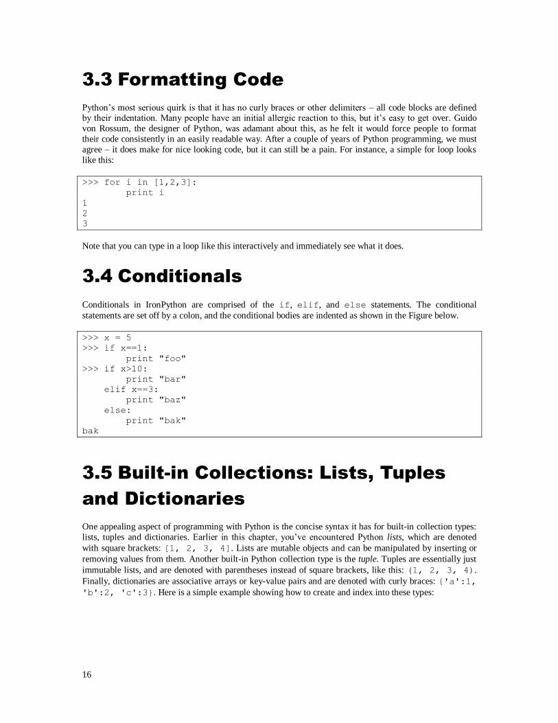
agree – it does make for nice looking code, but it can still be a pain. For instance, a simple for loop looks
like this:
>>> for i in [1,2,3]:
print i
1
2
3
Note that you can type in a loop like this interactively and immediately see what it does.
3.4 Conditionals
Conditionals in IronPython are comprised of the if, elif, and else statements. The conditional
statements are set off by a colon, and the conditional bodies are indented as shown in the Figure below.
>>> x = 5
>>> if x==1:
print "foo"
>>> if x>10:
print "bar"
elif x==3:
print "baz"
else:
print "bak"
bak
3.5 Built-in Collections: Lists, Tuples
and Dictionaries
One appealing aspect of programming with Python is the concise syntax it has for built-in collection types:
lists, tuples and dictionaries. Earlier in this chapter, you‟ve encountered Python lists, which are denoted
with square brackets: [1, 2, 3, 4]. Lists are mutable objects and can be manipulated by inserting or
removing values from them. Another built-in Python collection type is the tuple. Tuples are essentially just
immutable lists, and are denoted with parentheses instead of square brackets, like this: (1, 2, 3, 4).
Finally, dictionaries are associative arrays or key-value pairs and are denoted with curly braces: {'a':1,
'b':2, 'c':3}. Here is a simple example showing how to create and index into these types:

17
>>> l = [1, 2, 3, 4]
>>> t = ('a', 'b', 'c')
>>> d = {'a':1, 'b':2, 'z':26}
>>> l[0] # access first element of l
1
>>> t[0] # access first element of t
'a'
>>> d['a'] # look up the value bound to „a‟
1
>>> l[0] = 'howdy' # set an existing entry in a list
>>> l
['howdy', 2, 3, 4]
>>> t[0] = 123 # tuples are read-only, you can‟t change their values
Error: 'tuple' object is unsubscriptable
>>> l.append('bye!') # you can append values to a list, however
>>> l
['howdy', 2, 3, 4, 'bye!']
>>> d['a'] = 'one' # replace a value in a dictionary
>>> d['foo'] = 'bar' # add a new value
>>> d # note that the ordering of a dict may change
{'b': 2, 'z': 26, 'a': 'one', 'foo': 'bar'}
>>> l[-1] # you can use negative indices in tuples and lists
4 # in order to access elements starting from the end
>>> l[-2]
3
>>> t[-1]
'c'
You can use the keyword in to test if a value exists in a collection. Note that in looks at the keys, not the
values in a dictionary.

18
>>> li = [1,2,3]
>>> 2 in li
True
>>> 9 in li
False
>>> t = (1,2,3)
>>> 2 in t
True
>>> 9 in t
False
>>> d = {'a':1, 'b':2, 'c':3}
>>> 'a' in d
True
>>> 'x' in d
False
>>> 2 in d
False
3.6 Loops and Iterators
Loops are easy in IronPython using the “in” keyword. In fact, you can iterate over any IEnumerable
type in .NET, as we‟ll show below. The other function you need to know for simple loops is
range(start, end, step), which creates a list from start to just before end. Here are some
examples of common loop constructs:
>>> for x in [1,2,3]:
>>> print x
1
2
3
>>> for x in range(1,4):
>>> print x
1
2
3
>>> x = 1
>>> while x<4:
print x
x = x+1
1
2
3
As promised, you can also iterate over arbitrary IEnumerables:

19
>>> di = System.IO.DirectoryInfo(".")
>>> for f in di.GetFiles():
print f
dlmread.dll
imatrix.dll
IronMath.dll
IronPython.dll
...
3.7 Manipulating Lists
Python has some powerful mechanisms for manipulating lists; we give a brief overview of the most useful
tools here.
3.7.1 List Comprehensions
There is a very concise syntax for expressing operations that take lists (or any other enumerable collection,
really) as input and produce a list as output. These operations, called list comprehensions, look a little bit
like the first part of a for loop enclosed in square brackets. An example:
>>> [2*x for x in [1, 2, 3, 4]]
[2, 4, 6, 8]
This simple form of a list comprehension creates a new list by processing each element in an input list. It is
also possible to filter out items if you want to only operate on parts of the list:
>>> [x for x in [1, 2, 3, 4] if x%2==0]
[2, 4]
Note that if you iterate over a dictionary, the values you see will be the keys in the dictionary:
>>> [x+x for x in {'a':1, 'b':2}]
['aa', 'bb']
3.7.2 List
List simply takes any enumerable series and makes it into a list. This is particularly useful for hard-to-see
objects like the keys in a hashtable:

20
>>> h = System.Collections.Hashtable()
>>> h['a'] = 1
>>> h['b'] = 2
>>> h['c'] = 3
>>> list(h.Keys)
['a', 'b', 'c']
3.7.3 Zip
Zip lets you take multiple lists and “zip” them together, pairing the first element of the first list with the
first element of the others, and so on:
>>> zip(['a','b','c'],[1,2,3])
[('a', 1), ('b', 2), ('c', 3)]
3.7.4 Sort
Sort lets you sort a list (no surprise there), optionally passing in a comparison function of your choice that
compares two elements in the list. If you like, you can define the sort function inline via a lambda
expression (anonymous function):
>>> h = {'a':1, 'b':2, 'c':3, 'd':4}
>>> z = zip(list(h.Keys), list(h.Values))
>>> z
[('d', 4), ('b', 2), ('c', 3), ('a', 1)]
>>> z.sort()
>>> z
[('a', 1), ('b', 2), ('c', 3), ('d', 4)]
>>> z.sort(lambda a,b: a[1] < b[1])
>>> z
[('d', 4), ('c', 3), ('b', 2), ('a', 1)]
3.8 Dictionaries and Hashtables
There are two common types of hashtables available to you in Sho that can have arbitrary mixtures of types
for their keys and values: Python‟s dicts, which you have already seen, and .NET‟s
System.Collections.Hashtables. Both work in very similar ways:

21
>>> d = dict()
>>> d["a"] = 1
>>> "a" in d
True
>>> d["a"]
1
>>> h = System.Collections.Hashtable()
>>> h["dog"] = 1
>>> h["cat"] = 2
>>> h["giraffe"] = 3
>>> for key in h.Keys: print key, h[key]
dog 1
giraffe 3
cat 2
Of course, if you have consistent types for your keys and values, you can use the .NET generic type,
System.Collections.Generic.Dictionary; we‟ll discuss how to use generics in the next
section.
3.9 Using .NET Generics
If you‟d like to use .NET generics like System.Collections.List<int>, the syntax is a little
different in IronPython from what you may be used to in C# - instead of angle brackets, you need to use
square brackets ([int]) to specify the type.
>>> l = System.Collections.Generic.List[int]()
>>> l.Add(1)
>>> l.Add(2)
>>> l
List[int]([1, 2])
3.10 Functions
Defining a function is done with the def keyword. Here‟s a simple example:
>>> def myfunc(x):
return(x+1)
>>> myfunc(1)
2
We can call myfunc with arbitrary arguments, but not all arguments will provide the desired results!

22
>>> myfunc("a")
Error: unsupported operand type(s) for +: 'str' and 'int'
at myfunc$687$41.myfunc$687(PythonFunction $function, Object x) in
<string>: on or before line 2
at myfunc: line 2
3.10.1 Default Values and Named Arguments
It‟s often convenient to give parameters default values. This is simple and clean in IronPython:
>>> def myfunc(x=1, y=2):
return x*x+y
>>> myfunc()
3
>>> myfunc(2)
6
You can also specify which argument you‟re passing in:
>>> myfunc(y=3)
4
3.10.2 Function Pointers and Delegates
Passing function pointers around in Sho is as easy as defining the function itself. Using the example above,
we can now do the following:
>>> def dofunc(func, arg1, arg2):
return(func(arg1, arg2))
>>> dofunc(myfunc, 3, 3)
12
Internal to IronPython, these function pointers are delegates, so in some cases you can also use them to pass
functions into .NET code. For instance, to override behavior for a .NET Form, you can just add a handler
from Python using the function pointer:
>>> def onclick(obj, mouseeventargs):
print "got a click!"
>>> f = Form()
>>> f.Click += onclick
For more information on using delegates with Forms, see the chapter “Writing GUIs with Sho.”
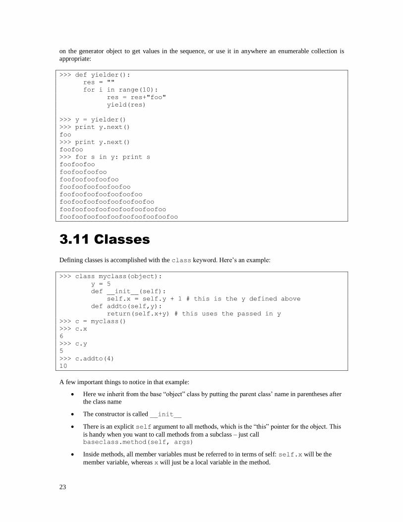
3.10.3 Yield
They say it‟s better to give than receive, so if you‟re tired of consuming and manipulating lists made by
others, you can produce enumerable lists with the yield command. Yield is like a fancy version of “return”
that produces an enumerator object (called a generator in Python parlance). You can call the next method
23
on the generator object to get values in the sequence, or use it in anywhere an enumerable collection is
appropriate:
>>> def yielder():
res = ""
for i in range(10):
res = res+"foo"
yield(res)
>>> y = yielder()
>>> print y.next()
foo
>>> print y.next()
foofoo
>>> for s in y: print s
foofoofoo
foofoofoofoo
foofoofoofoofoo
foofoofoofoofoofoo
foofoofoofoofoofoofoo
foofoofoofoofoofoofoofoo
foofoofoofoofoofoofoofoofoo
foofoofoofoofoofoofoofoofoofoo
3.11 Classes
Defining classes is accomplished with the class keyword. Here‟s an example:
>>> class myclass(object):
y = 5
def __init__(self):
self.x = self.y + 1 # this is the y defined above
def addto(self,y):
return(self.x+y) # this uses the passed in y
>>> c = myclass()
>>> c.x
6
>>> c.y
5
>>> c.addto(4)
10
A few important things to notice in that example:
Here we inherit from the base “object” class by putting the parent class‟ name in parentheses after
the class name
The constructor is called __init__
There is an explicit self argument to all methods, which is the “this” pointer for the object. This
is handy when you want to call methods from a subclass – just call baseclass.method(self, args)
Inside methods, all member variables must be referred to in terms of self: self.x will be the
member variable, whereas x will just be a local variable in the method.

24
You can declare a class variable either in the constructor or in the body of the class definition
(outside of any method definition).
If you are inheriting from something more interesting than just object, you can directly call methods on
the superclass by directly calling its methods, as seen in the constructor below. Note you can subclass .NET
classes as well as IronPython classes.
>>> class subclass(myclass):
def __init__(self):
self.y = 4
myclass.__init__(self)
def addmore(self, z):
return(self.x+self.y+z)
>>> s = subclass()
>>> s.x
5
>>> s.y
4
>>> s.addmore(5)
14
3.12 Files and Namespaces
Once you get beyond trivial files and functions, you‟ll want to start putting your IronPython code into files.
For example, let‟s say you put the following code into myfile.py:
# myfile.py
foo = 4
bar = "test"
class myclass:
def __init__(self):
self.x = 3
def addto(self,y):
return(self.x+y)
def testfunc(x):
return(2*x)
First you‟ll need to make sure myfile.py is in your IronPython path (which is stored in a variable called
sys.path); you can extend the path via the Sho function addpath(dir). There are now three ways to
use this code: execfile, import, and “from <module> import <symbol>.” We describe each
method below:
3.12.1 Execfile
The execfile(filename) function interprets the file as though you‟d typed it in. This is the classic
“scripting” model:

25
>>> execfile("myfile.py")
>>> foo
4
>>> testfunc(2)
4
This is convenient when you‟re doing the same thing over and over again, but too much of it leads to poor
modularity. If you find yourself doing this a lot or on really long files, you should start thinking about
making them into modules and importing them, as we discuss below.
Note that execfile does not search through the IronPython path, so you‟ll have to either cd to the
proper directory or fully qualify the filename.
3.12.2 Import
Import interprets everything in the file and puts it into a namespace that defaults to the filename root. All
variables, classes, and functions are accessible, but must be qualified with this namespace. For instance:
>>> import myfile
>>> foo
Error: name 'foo' not defined
Stack Trace: IronPython.Runtime.Exceptions.PythonNameErrorException:
name 'foo' not defined
>>> myfile.foo
4
>>> myfile.testfunc(2)
4
Now let‟s say you edit myfile.py to change the behavior of some function. You‟d think you can just import
again, right? Python doesn‟t work that way, and it‟s actually to make things more efficient – if you have a
bunch of modules that are importing the same module, this prevents multiple re-interpretings. To force an
update, you have to use the reload command:
>>> myfile.foo
4
# now update myfile.py so that foo = 5
>>> reload(foo)
<module myfile from "C:\test\myfile.py">
>>> myfile.foo
5
Python files can themselves import other modules (and must, if they want to use other functionality). Such
modules, then, will exist inside the namespace of the module you‟ve imported. Let‟s say myfile.py imports
yourfile, and yourfile implements a function called bar. Then if you import myfile, bar can be accessed as
myfile.yourfile.bar. If that‟s inconvenient, of course you can import bar at the top level.
Another subtlety to keep in mind is that reload does not work recursively. Thus, if myfile imports yourfile
as above, and you edit/save yourfile.py, calling reload(myfile) will not update the behavior of
yourfile. To do that you‟ll have to do reload(myfile.yourfile). If you‟ve updated myfile as well,
you‟ll then have to reload(myfile).
If you‟re not happy with the default name of your module, you can change it with the as keyword. This is
especially useful for collapsing multilevel namespaces:

26
>>> import myfile as mymod
>>> mymod.foo
4
>>> import System.Windows.Forms as WinForms
>>> f = WinForms.Form()
3.12.3 From <module> import <symbol>
The final way to use items from a file is to import them individually or en masse into the top level. For instance, if you just want to pull in foo from myfile.py, you can do:
>>> from myfile import foo
>>> foo
4
If you want to pull in all the symbols into the top level namespace, you can use “*”:
>>> from myfile import *
>>> foo
4
Reloading in this case is trickier, since the module‟s name has never been added to the global namespace.
You thus have to import the module, reload it, and then import * from it again. This has a nice
little rhythm to it, which makes it easier to remember:
import foo,
reload foo,
from foo import star!
3.13 Exceptions
Exception handling in Python works beautifully with exception handling in .NET. Essentially, .NET
exceptions are passed up to IronPython and can be dealt with from the interpreter level. As shown below,
you can catch a particular exception with try: <block> except exceptionname:, or catch them
all with except:. Here‟s how it works:
>>> try:
print a
except NameError:
print "a is not defined!"
unknown error: name 'a' is not defined
>>> try:
a = "foo"+234
except:
msg, stacktrace = geterror()
print message
unsupported operand type(s) for +: 'str' and 'int'

27
Note that the geterror() function returns both the error message and the stack trace; the latter contains
line number information and can be quite helpful if the error is occurring in a function or method defined in
a module.
You can also create your own exceptions via the raise(obj) command, where obj can be a class or
instance. It‟s best to use System.Exception objects or derive your own exceptions from that; that way the usual exception-processing pipeline will be able to handle your exceptions:
>>> raise System.Exception("something went terribly, terribly wrong")
Error: something went terribly, terribly wrong
3.14 ShoThreads
IronPython does not have its own threads, but Sho has a threading facility, called ShoThreads, based on the
native .NET threading model. While it is possible to use .NET threads directly, we recommend against this,
since an exception in a raw .NET thread will break all of IronPython. ShoThreads catch any errors and print them to the console. ShoThreads also allow you to specify a tag, so you have anonymous threads you need
to kill or otherwise manage you can find them with lsShoThreads().
For instance, we can define a simple loop and put it in a thread:
>>> def loop():
while True:
print "foo"
System.Threading.Thread.Sleep(100)
>>> t = ShoThread(loop, "test thread")
>>> t.Start()
foo
foo
foo
>>> t.Abort()
Some useful things to know about ShoThreads:
The function you pass in to the constructor can‟t take any arguments
Once you start a thread, you‟ll get back control of the command prompt
You can list currently running ShoThreads via the lsShoThreads() command
You can kill an individual ShoThread via killShoThreadByIndex(index)
You can set the ApartmentState to STA or MTA using the third argument to the constructor
Here‟s another example, showing how to put up a .NET Form in its own thread in just three lines of code:
>>> f = System.Windows.Forms.Form(Text="hello world")
>>> t = ShoThread(f.ShowDialog)
>>> t.Start()
Below we show the resulting window, which you can move around, refresh, iconify, close, etc. (since the
thread is running the message pump with ShowDialog).

28
Figure 3.1: A .NET Form in its own thread in three lines of code.

29
Chapter 4: Matrix Classes
By and large, Sho uses .NET classes. However, Sho introduces an important set of classes for data analysis:
the matrix classes. Sho contains typed array classes to hold doubles (DoubleArray,
SparseDoubleArray), floats (FloatArray, SparseFloatArray), ints (IntArray,
SparseIntArray) and complex numbers (ComplexArray) , as well as a non-numeric array that holds
arbitrary managed .NET Objects (ObjArray, SparseObjArray) and Booleans (BoolArray,
SparseBoolArray.) Included with the array datatypes are a rich set of methods and functions to
manipulate array values and perform mathematical operations on them. Many of these math operations (the
linear algebra classes in particular) are accelerated via MKL, Intel‟s implementation of the BLAS linear
algebra package.
Let‟s take a look at some of the array functionality in Sho, concentrating on DoubleArrays, which have
the most math functionality.
4.1 Array Creation
You create a 1-D, 2-D, or multidimensional array using the DoubleArray constructor:
>>> x = DoubleArray(10)
# creates a 1 x 10 array (row vector)
>>> A = DoubleArray(10, 12)
# creates a 10 x 12 2-D array
>>> A = DoubleArray(3, 4, 5)
# creates a 3 x 4 x 5 multidimensional array
Note that if you want to create a column vector, you need to create an array with one column.
>>> b = DoubleArray(10, 1)
# creates a 10 x 1 array (column vector)
You can get the number of rows and columns from the array‟s Size property, or get at them individually
with size0 or size1 (for 2-D arrays):
>>> b.Size
Array[int]((1, 10))
>>> b.size0
1
You can also create DoubleArrays out of things that look 1D or 2D array-like (specifically,
IEnumerable or IEnumerable of IEnumerables) using the From method. So, you can make one
out a Python array:
>>> DoubleArray.From([1,2,3,4])
[ 1.0000 2.0000 3.0000 4.0000]
You can use this to make two-dimensional or even multi-dimensional arrays as well, by grouping elements
appropriately.

30
>>> DoubleArray.From([[1,2],[3,4]])
[ 1.0000 2.0000
3.0000 4.0000]
>>> a = DoubleArray.From([ [[1,2],[3,4]] , [[5,6],[7,8]] ])
# returns a 2x2x2 array
>>> a[0,:,:].Squeeze()
[ 1.0000 2.0000
3.0000 4.0000]
>>> a[1,:,:].Squeeze()
[ 5.0000 6.0000
7.0000 8.0000]
The utility functions eye and ones let you quickly create identity matrices and matrices filled with ones.
>>> eye(3,3)
[ 1.0000 0.0000 0.0000
0.0000 1.0000 0.0000
0.0000 0.0000 1.0000]
To create matrices out of other matrices, you can use the <type>Array.HorizStack and
<type>Array.VertStack commands:
>>> DoubleArray.HorizStack(eye(2,2), eye(2,2))
[ 1.0000 0.0000 1.0000 0.0000
0.0000 1.0000 0.0000 1.0000]
>>> DoubleArray.VertStack(eye(2,2), eye(2,2))
[ 1.0000 0.0000
0.0000 1.0000
1.0000 0.0000
0.0000 1.0000]
You can easily create matrices full of random numbers using the rand, randn and randint
functions, to produce arrays of uniformly or Gaussian-distributed doubles, or uniformly-distributed integers
in a given range:
>>> rand(3, 3)
[ 0.2886 0.7908 0.5283
0.8500 0.2996 0.2847
0.5477 0.8334 0.1295]
>>> randn(3, 3)
[-0.3155 0.8782 -0.9785
-1.0173 -0.4855 1.3568
-0.3304 -1.0168 0.7422]
>>> randint(3, 3, 100)
[ 68 93 93
73 32 87
4 93 59]
To fill an existing array with random numbers, use the FillRandom method, which requires you to
supply a random number generator object.
>>> A.FillRandom(System.Random())

31
4.2 Element Access and Slicing
You can do element-wise reads/write of the matrix, although this is slow compared to the slicing methods
below. Notice that Sho uses 0-based indexing, so A[3,4] is really the element in the fourth row and the
fifth column.
>>> A[3, 4] = 4.5
>>> A[3, 4]
4.5
You can read/write more than one element at a time with the slicing syntax. The “:” operator means “all,”
so A[3,:] means all elements of A with row==3 and col==all. In other words, we get back the entire
fourth row:
>>> A[3, :]
[ 0.6266 0.9795 0.0853 0.0776 4.5000 0.5372 0.8158 0.3565 0.8322 0.7706
0.1115 0.1214]
This returns a “shallow copy,” i.e., what you get back is a view of your original data instead of a copy of
that data. This makes things much more memory efficient, since the underlying data is not copied. It does
have some important implications, though, which we‟ll discuss at the end of this section.
Beyond specifying all elements for slices, you can also specify ranges, for instance columns 0 up to (but
not including) 2 of row 3:
>>> A[3, 0:2]
[ 0.6266 0.9795]
Or, all rows of column 5:
>>> A[:, 5]
(printout of 10-element column vector suppressed)
Even fancier, you can skip elements. For example, row 3, columns 0 up to (but not including) 8, skip by 2:
>>> A[3, 0:8:2]
[ 0.6266 0.0853 4.5000 0.8158]
You can also access arbitrary subsets of rows or columns using lists (note: unlike other slicing operations,
this makes a deep copy):
>>> A[[3, 2], 0:4]
[ 0.6266 0.9795 0.0853 0.0776
0.9377 0.8708 0.2750 0.6975]
And, all of these expressions can serve as left-hand sides:
>>> A[3, :] = A[4, :]
>>> A[3, 3]
0.697456899424
>>> A[4, 3]
0.697456899424
32
And, you can do extra fancy stuff with both row and column specifiers:
>>> A[3:5:2, 3:5:2] = A[4:6:2, 4:6:2]
For 1D arrays, you can access elements in the same way, but only need one index:
>>> b = rand(10)
>>> b[:5]
[ 0.2850 0.4686 0.3585 0.6589 0.0573]
>>> b[0:8:3]
[ 0.2850 0.6589 0.9287]
Now back to the implications of slices being “shallow:” since what you get back is a view of the underlying
data and not a copy of that data, changes to the slice will change the original array you sliced from as well!
The example below shows the implications of this:
>>> >>> A = eye(3,3)
>>> b = A[:,0] # b is a shallow version of part of A
>>> b[0] = -1
>>> A
[-1.0000 0.0000 0.0000
0.0000 1.0000 0.0000
0.0000 0.0000 1.0000]
4.3 Optimized Matrix Methods
Sho contains three optimized methods for common operations, MultiplyTranspose, MultiplyAccum and
MultiplyInto.
MultiplyTranspose is used to compute or . The Boolean flag specifies whether the
transposed array is first (flag is true) or second (flag is false).
>>> A = rand(10,10)
>>> B = A.MultiplyTranspose(True) # B = A.T * A
>>> C = A.MultiplyTranspose(False) # C = A * A.T
MultiplyAccum is used to compute where is a scalar.
>>> A = rand(10,10)
>>> B = rand(10,10)
>>> A.MultiplyAccum(3.0, B) # A = A + 3.0 * B
MultiplyInto is used to compute ( ) ( ) , where and are scalars and (T) denotes an optional transpose. This method maps directly into MKL‟s gemm, so it more efficient than the code that
uses operators because it bypasses the copying incurred by using operators.
There are two overloads of this method. The two-parameter version computes , storing the result in
the already allocated matrix .

33
>>> A = zeros(10,10)
>>> B = rand(10,10)
>>> C = rand(10,10)
>>> A.MultiplyInto(B,C) # A = B * C, but A is not re-allocated
The six-parameter version computes ( ) ( ) , where (T) is specified by flags (equal to true if
transpose, false otherwise).
>>> A = rand(10,10)
>>> B = rand(10,10)
>>> C = rand(10,10)
>>> # Compute A = 3.0 * B * C.T + 4.5 * A
>>> A.MultiplyInto(3.0, B, False, C, True, 4.5)
4.4 Sparse Arrays
Sho also includes support for computation using sparse arrays. To create a sparse array, use the
Sparse<type>Array factory methods, which work analogously to the array factory methods described
above:
>>> sa = SparseDoubleArray(100, 100)
In addition to the normal ways of iterating through an array, sparse arrays have enumerators like
Elements that allow you to iterate over just the entries in the array that have had values assigned to them.
>>> sa[1, 1] = 1.0
>>> sa[3, 4] = 2.0
>>> sa[5, 6] = 3.0
>>> for x in sa.Elements: print x.Row, ",", x.Col, ":", x.Value
1 , 1 : 1.0
3 , 4 : 2.0
5 , 6 : 3.0

34
The standard math operators have been implemented for sparse arrays:
>>> sa1 = SparseDoubleArray(10000, 10000)
>>> sa2 = SparseDoubleArray(10000, 10000)
>>> sa1[1, 1] = 10
>>> sa1[1, 1] = 1
>>> sa1[1, 2] = 2
>>> sa2[1, 1] = 10
>>> sa2[2, 1] = 20
>>> sa3 = sa1*sa2
>>> for x in sa3.Elements: print x
[1,1 -> 50]
Note that the implementation of sparse arrays trades off some compactness in the representation for speed
in accessing elements. Therefore, an m×n array with N nonzero elements uses memory proportional to n
plus N.
4.5 Multidimensional Arrays
Sho has support for multidimensional arrays; we‟ve already seen how to construct them, and now go
through some of the operations they support. We can slice and dice them as with 1D or 2D arrays.
>>> A = DoubleArray(3, 3, 3)
>>> A.FillRandom(System.Random())
>>> A[:, :, 2]
[[0.5097 0.0605 0.3288]
[0.4535 0.9987 0.0312]
[0.1063 0.8235 0.5403]]
The result is 1x3x3 array. In order to use it in ordinary linear algebra operations as a 3x3 matrix, we need
to “squeeze” out the size 1 dimensions:
>>> A[:, :, 2].Squeeze()
[ 0.5097 0.4535 0.1063
0.0605 0.9987 0.8235
0.3288 0.0312 0.5403]
We can also add, multiply, etc. two arrays. However, note that only the elementwise operations are
available for multidimensional arrays, as the others are not mathematically well-defined:
>>> B = rand(3, 3, 3)
>>> C = A+B
>>> C = A.ElementMultiply(B)

35
4.6 Group and Elementwise Operations
There are a variety of aggregation methods that operate either on all elements, all rows, or all columns:
>>> A.Min()
0.00572715467109
>>> A.Min(OverCol) # min along columns, one per row
[ 0.1427
0.0457
0.0223
0.1235
0.1104
0.0793
0.1203
0.0349
0.0057
0.0442]
>>> A.Min(OverRow) # min along rows, one per column
[ 0.0606 0.1262 0.0457 0.0349 0.0057 0.1203 0.0223 0.1644 0.1235
0.0793]
There are two alternative ways of specifying directions for aggregation functions: OverCol/OverRow ,
which runs the aggregation function over each direction; EachCol/EachRow, which produces an answer
once for each direction. For 2D matrices OverCol is equivalent to EachRow, and OverRow is equivalent to
EachCol.
Other methods that work this way include Max, Mean, Median,Std (standard deviation), Var
(variance), and VarN (variance normalized by N.) Additionally, many basic unary math functions have
been overloaded to work on each element of an array:
>>> b
[ 0.2850 0.4686 0.3585 0.6589 0.0573 0.4675 0.9287 0.6721 0.1266
0.0844]
>>> exp(b)
[ 1.3297 1.5978 1.4311 1.9326 1.0589 1.5961 2.5313 1.9583 1.1349
1.0880]
Arrays provide special element-wise comparison operators that return integer matrices. In the example
below, we use the ElementLT method to see which of the elements of A are less than 0.5. Note that
ElementLT can also be abbreviated with the “<” symbol. Enter help("matrix") for a full list of
elementwise operations.

36
>>> A = rand(3, 4)
>>> A
[ 0.2657 0.2968 0.0606 0.1262
0.3873 0.9614 0.0057 0.1781
0.7405 0.5911 0.9570 0.3714]
>>> A.ElementLT(0.5)
[ 1 1 1 1
1 0 1 1
0 0 0 1]
>>> A<0.5
[ 1 1 1 1
1 0 1 1
0 0 0 1]
4.7 The Find Command
The Find command can be used to find elements of an array that satisfy some condition:
>>> for x in Find(A<0.5): print A[x]
0.265678072472
0.296778736309
0.0605958090446
0.12621970434
0.387283846916
0.00572715467109
0.178092201789
0.371449938683
Note that this iterator also contains the row and column information for each element:
>>> for x in Find(A<0.5):
print x.Row, x.Col, A[x]
0 0 0.2657
0 1 0.2968
0 2 0.0606
0 3 0.1262
1 0 0.3873
1 2 0.0057
1 3 0.1781
2 3 0.3714
Note we could have used x.Value instead of A[x]. You can also quickly set a subset of the elements of
an array that have some property:
>>> A[Find(A<0.5)] = 0.5
>>> A
[ 0.5000 0.5000 0.5000 0.5000
0.5000 0.9614 0.5000 0.5000
0.7405 0.5911 0.9570 0.5000]

37
4.8 Linear Algebra
In addition to slicing and dicing matrices, DoubleArray and FloatArray can perform the usual linear
algebra operations of adding, subtracting and multiplying, as long as the matrix dimensions line up (note
that only elementwise operations are available for multidimensional arrays). You can also add, subtract,
multiply, and divide by scalars. For example,
>>> A = rand(10, 10)
>>> b = rand(10, 1)
>>> c = rand(1, 10)
>>> d = (A.T*b+c.T)/2+1
>>> d
[ 2.3506
2.9228
3.1646
2.6282
3.1403
2.8749
2.8998
3.0028
2.4706
3.1772]
Note that the T property returns a shallow copy (a view) of C, with rows and columns transposed, i.e., it
doesn‟t make a deep copy of the elements; it just reinterprets them with row and column indices swapped.
This makes transposing fast, but note that if you modify C.T you‟ll be modifying C as well.
Sho has extra classes that do advanced linear algebra operations on matrices. For example, if you want to
solve a linear system , you can use the LU decomposition class:
>>> A = rand(10, 10)
>>> b = rand(10, 1)
>>> decomp = LU(A)
>>> x = decomp.Solve(b)
>>> norm(A*x-b, 1)
2.40779618466e-015
decomp is now an LU object – you can use doc to find out more about its methods. Also, notice that here
we made a temporary DoubleArray with no name ( ), and called the norm function on it with an
argument of 1, which computes the L1 norm of the vector.
The linear algebra classes currently include the following:
1) LU (LU, LUFloat, SparseLU),
2) QR (QR, QRFloat),
3) Schur (Schur, SchurFloat),
4) Cholesky (Cholesky, CholFloat, SparseCholesky),
5) SVD (SVD, SVDFloa, SingularVals, SingularValsFloat),
6) Eigenvalue (Eigen, EigenSym, EigenAsym, EigenFloat, EigenSymFloat,
EigenAsymFloat, EigenVals, EigenValsFloat, EigenValsAsym,
EienValsAsymFloat, EigenValsSym, EigenValsSymFloat)
7) A generic dense solver (Solver)

38
SVD and eigenvalue both include classes (SingularVals, EigenVals) for computing just the
singular or eigen values; use these if you do not need the full decomposition, as they will be faster and
more memory efficient.
The following is an example of using the linear algebra classes:
>>> s = SVD(A)
>>> A_hat = s.U * s.D * s.V.T
>>> norm(A-A_hat, 1)
1.26426646929e-014
Notice here that the SVD class has 3 properties: U (the left singular vectors), D (the diagonal matrix of
singular values), and V (the right singular vectors).
In addition to the specialized linear algebra classes, the inv and det functions return the inverse and
determinant of an array:
>>> norm(A*inv(A) - eye(10,10))
1.3079625534173405e-14
>>> det(A*inv(A))
1.000000000000006
The generic solver class, Solver, attempts to solve the system by the most appropriate method. After
solving, you can check the property MethodUsed to see which method was utilized.
For square matrices, the system will be solved by one of the following methods:
1) Cholesky if the matrix is positive-definite. 2) LU if the matrix is not positive-definite and is not rank deficient.
3) SVD if the matrix is rank deficient.
For non-square matrices, the system is over or underdetermined. In this case, the system will be solved
either by
1) QR if the matrix is not rank-deficient or
2) SVD if the matrix is rank-deficient.
>>> a = rand(10,10)
>>> c = a * a.T
>>> s = Solver(c)
>>> x = rand(10,1)
>>> b = c * x # create a right hand side
>>> s = Solver(a)
>>> y = s.Solve(b) # we should get the same as x
>>> s.MethodUsed
ShoNS.Array.SolverMethod.SolveChol # the Cholesky method was used
>>> (x – y) # if zeros, we found the solution
(printout of 10-element column vector full of zeros suppressed)

39
Chapter 5: Math and Data
Analysis
5.1 Mapping functions
There‟s a fair amount of math functionality in Sho that is not tied to the matrix classes – that is, you can mathematically munge collections that contain doubles, without having to convert to Sho arrays (but, these
functions often produce Sho arrays). For example:
>>> sin([1,2,3,4])
[ 0.8415 0.9093 0.1411 -0.7568]
>>> sqrt([1,2,3,4])
[ 1.0000 1.4142 1.7321 2.0000]
Unlike the Python standard sin and sqrt functions, these take any IEnumerable collection, map the
function over it, and produce a DoubleArray. Sho provides lots of functions like this: abs, acos,
asin, atan, atan2, ceil, cos, cosh, exp, floor, log, log10, pow, round, sign, sin, sinh,
sqrt, tan, tanh and trunc .
If you want to apply your own function to all elements of a DoubleArray, you can use the ApplyFunc
command:
>>> def doubler(x): return 2*x
>>> ApplyFunc(DoubleArray.From([1,2,3,4,5]), doubler)
[ 2.0000 4.0000 6.0000 8.0000 10.0000]
You can also use ApplyFunc to create functions of two arrays of the same size, where each element of
the returned array is a function of the corresponding elements from each of the two input arrays:
>>> def adder(x,y): return x+y
>>> ApplyFunc(eye(2,2), eye(2,2), adder)
[ 2.0000 0.0000
0.0000 2.0000]
5.2 Stepping through intervals
Another Sho improvement to standard Python is the drange object. drange represents an interval of real
numbers that is divided into equal sized steps, like Python‟s range and xrange. However, unlike
Python‟s range and xrange, which only take integers as arguments, drange takes doubles. You can
also specify the number of elements by using the keyword Count as below.

40
>>> DoubleArray.From(drange(2, 4.5)) # default step size of 1
[ 2.0000 3.0000 4.0000]
>>> DoubleArray.From(drange(2.1, 2.6, 0.1)) # specify a step of 0.1
[ 2.1000 2.2000 2.3000 2.4000 2.5000 2.6000]
>>> DoubleArray.From(drange(1.0, 2.0, Count=10)) # specify 10 elements
[ 1.0000 1.1111 1.2222 1.3333 1.4444 1.5556 1.6667 1.7778 1.8889
2.0000]
drange is a .NET IEnumerable object, so you can loop over it:
>>> d = drange(0, 1, 0.01)
>>> s = 0
>>> for x in d:
s = s+x
>>> s
50.5
You can also tweak its parameters, and even add, subtract, and multiply it by scalars:
>>> d.Begin = -1
>>> d.Step = 0.1
>>> d
[-1:0.1:1]
>>> e = (d*2-1)/4
>>> e
[-0.75:0.05:0.25]
5.3 Histogramming
The Histogram class buckets data into a set of consecutive bins (a related function we‟ll see in the next
chapter is hist() which both creates and plots the histogram):
>>> h = Histogram(A)
Histogram automatically chooses buckets and counts the number elements in the input collection that
fall into that bucket:
>>> h.Count
System.Int32[](2, 7, 13, 12, 19, 17, 11, 12, 6, 1)
>>> h.BinCenter
System.Object[](-1.87989378990, -1.45514758655, -1.03040138320, -
0.605655179848, -0.180908976497, 0.243837226854, 0.668583430206,
1.09332963356, 1.51807583691, 1.94282204026)
You can also change the number of bins with an optional second argument
>>> h = Histogram(A, 20)
>>> h.Count
System.Int32[](2, 0, 4, 3, 7, 6, 3, 9, 12, 7, 7, 10, 5, 6, 6, 6, 2, 4,
0, 1)

41
Or specify the bin centers, instead, with a second argument that is array-like:
>>> h = Histogram([1,1,1,4,5], [1,4])
>>> h.Count
System.Int32[](3, 2)
If the data in the input collection is discrete, the bins become exact, rather than ranges:
>>> a = ['abc', 'abc', 'def', 'ghi']
>>> h = Histogram(a)
>>> h.BinCenter
System.Object[]('abc','def','ghi')
>>> h.Count
System.Int32[](2, 1, 1)

42
Chapter 6: Data Handling
There are several ways to get data in and out of Sho. Remember that Sho is built on .NET, so any data
method that lives in .NET can be easily used from Sho (e.g., XML parsing in System.XML). in addition,
we provide some helper functionality that makes it easier for you to load and save data in Sho.
6.1 Pickling Sho data
Since Sho is designed to be an exploratory environment for playing with data, it needs quick a way to store
and retrieve that data. To that end, Sho provides a pair of functions that allow you to persist your data
(either to disk or to a memory-resident object). To store an object for later use, call the pickle function,
which takes as the first parameter, the object to store, and optionally a filename (if you want to store your
data on disk). You can then call unpickle to get the data back – pass either the filename you‟ve pickled the
data to or the object that was retured from pickle. Here is an example:
>>> a = rand(5)
>>> a
[ 0.4669 0.1889 0.4706 0.3542 0.7747]
>>> p = pickle(a)
>>> unpickle(p)
[ 0.4669 0.1889 0.4706 0.3542 0.7747]
>>> b = [(1,2), {'a':1}, (3,4)]
>>> b
[(1, 2), {'a': 1}, (3, 4)]
>>> pickle(b,"c:/b.dat")
>>> unpickle("c:/b.dat")
[(1, 2), {'a': 1}, (3, 4)]
Currently, Sho pickling is limited to the following data types:
Basic scalar data types
The basic Python collection types (lists, dicts, tuples)
Python xrange objects
Sho arrays
Basic .NET collection classes
Pure Python objects (but not Python classes inherited from .NET classes)
Anything else that supports .NET serialization
Combinations of the above
6.2 Reading/Writing Delimited Files
There are some built-in methods for improved data handling. For example, Sho allows you to read and
write .csv files:

43
>>> A = csvreadJaggedArray('foo.csv')
>>> A.GetType()
System.Object[]
>>> csvwrite('goo.csv', A)
Note that csvreadJaggedArray produces a native .NET object array (Object[]) that contains other
Object[]s (if there is only one row or column, it just returns an Object[]). If you want an
ObjArray, use csvreadArray, and if you want a DoubleArray, use csvreadDoubleArray (or
csvreadFloatArray, etc.).
If you want to read a file with a delimeter other than a comma, use one of the dlmread functions:
>>> A = dlmreadJaggedArray('foo.dat', '\t')
>>> dlmwrite('foo.dat','\t' ,A)
To read these into Sho arrays, use the dlmreadArray and dlmreadDoubleArray functions.
6.3 Reading from a Database
If you data is stored in a database, instead of a flat file, Sho has an easy mechanism for getting at your data
(if this mechanism is too limited, you can always call ADO.NET directly from Sho, too).
First, create a Sho database object:
>>> db = Database()
Second, connect to the database (below, “proxcard”, which is located on the machine “msr-sql01”).
>>> db.Connect('msr-sql01', 'proxcard')
This logs you in with your Windows credentials; if you want SQL credentials, add two more parameters:
username and password. Note that the two and four parameter versions of Connect use the defaults
“Persist Security Info=False;Integrated Security=SSPI.” If you need to specify different security settings,
use the one-parameter Connect method, in which you can pass in the exact connection string.
Next, specify the query you‟d like to execute; note that setting the query doesn‟t execute it.
>>> db.Command = 'select b.DemoTitle, count(*) as kount from
BadgeRead05 r join ReaderBoothLookup05 b on r.ReaderID = b.ProxReaderID
group by b.DemoTiltle order by kount desc'
Now you‟re ready to execute the query and get your data. You can get the data by row:
>>> x = db.DataByRow()
DataByRow returns all of the rows in the database, as a List[Array[object]]. Alternatively, you
can get the rows individually in a loop:
>>> while True:
x = db.ReadRow() # returns an object[]
if x == None: break
44
You can also use DataByCol, which returns one or more columns of the queries, as object[] (for one)
or object[object[]] (for multiple):
>>> x = db.DataByCol() # get all columns
>>> x = db.DataByCol(0) # get the first column (in order specified by
select statement)
>>> x = db.DataByCol([1,4]) # get the second and fifth columns
The database object is smart – it only executes the query once, when you first get the data. If you change
the command string, it will re-execute the string at the next opportunity.
6.4 Roll your own data readers/writers
Using IronPython, it isn‟t too difficult to create your own data readers and writers. You can use either the
Python file object (fast, IEnumerable, but ASCII only), or the .NET StreamReader/
StreamWriter classes (slower, handles Unicode with UTF-8).
6.4.1 Custom ASCII Data Reader
The example below shows the .NET way of doing things, reading a file line-by-line, applying a regular
expression match to each line, extracting out the matched expression and printing it:
>>> from System.IO import StreamReader
>>> from System.Text.RegularExpressions import Regex
>>> R = Regex('(\d+)')
>>> sr = StreamReader('c:/temp/data.dat')
>>> while True:
line = sr.ReadLine()
if line == None: break
m = R.Match(line)
if m.Success:
print m.Groups[1].ToString()
32234
562
6265
6.4.2 Custom Binary Data Reader
You can read binary data using the System.IO.BinaryReader class. There are a variety of utilities
in System.BitConverter to help you convert the bytes you read back into values. The example
below opens a file and reads a 4-character string, then grabs the next four bytes, reverses their order
(switching from little Endian big Endian), and converts them to an Int32.

45
>>> fs = System.IO.File.OpenRead(filename)
>>> br = System.IO.BinaryReader(fs)
>>> while (True):
res = br.ReadBytes(4)
id = System.Text.ASCIIEncoding().GetString(res)
print id
chunkarray = br.ReadBytes(4)
System.Array.Reverse(chunkarray)
chunklength = System.BitConverter.ToInt32(chunkarray, 0)
print chunklength
abcd
243
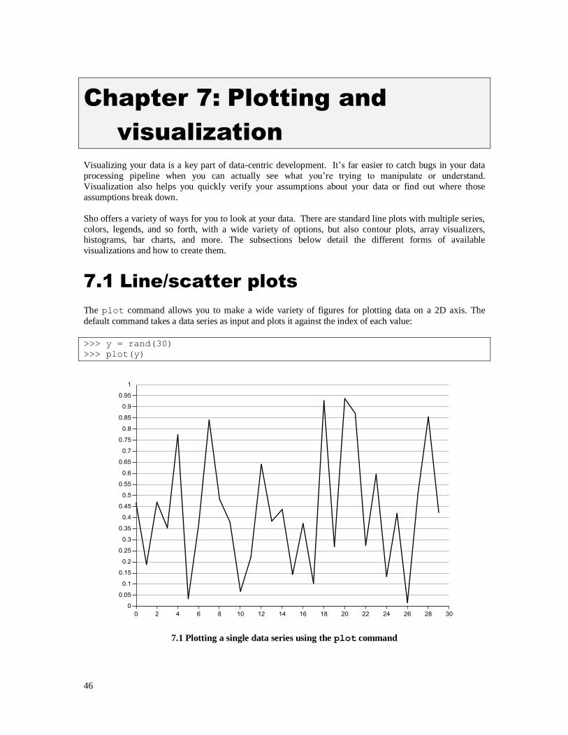
46
Chapter 7: Plotting and
visualization
Visualizing your data is a key part of data-centric development. It‟s far easier to catch bugs in your data
processing pipeline when you can actually see what you‟re trying to manipulate or understand.
Visualization also helps you quickly verify your assumptions about your data or find out where those
assumptions break down.
Sho offers a variety of ways for you to look at your data. There are standard line plots with multiple series,
colors, legends, and so forth, with a wide variety of options, but also contour plots, array visualizers, histograms, bar charts, and more. The subsections below detail the different forms of available
visualizations and how to create them.
7.1 Line/scatter plots
The plot command allows you to make a wide variety of figures for plotting data on a 2D axis. The
default command takes a data series as input and plots it against the index of each value:
>>> y = rand(30)
>>> plot(y)
7.1 Plotting a single data series using the plot command

47
You can also plot one data series versus another (if they‟re of the same length):
>>> x = rand(30)
>>> plot(x, y, '*')
7.2 Plotting two data series against one another
Note that in this case, instead of connecting all of the points (which is the default), we placed a star at every
data point, with no line between them. This third (optional) parameter specifies the color and shape of the
line and marker through shortcut characters. The color is specified by one character:
r = red
g = green
b = blue
k = black
y = yellow
c = cyan
m = magenta
w = white
The marker at each point is specified with one character (default is no marker):
+ = plus sign
o = dot
* = asterisk
. = dot
s = square
^ = triangle pointing up
v = triangle pointing down

48
When you specify a marker, Sho assumes you don‟t want to connect the markers. You can tell it to connect
with a line by adding one of the following character codes:
- = solid line
: = dotted line
-- = dashed line
-. = dash-dot line
Note that you can specify color, shape and/or line style by using a string with multiple characters. So, you
can get a blue line with connected square markers by using „bs-„ (or any other order). You can also plot
more than one series per plot, mixing and matching styles as you wish:
>>> plot(x, 'r^-', y, 'bo')
7.3 Plotting multiple series and styles of data on one set of axes

49
Each series is specified by either 1 or 2 collections, followed by an optional string of shape/color
commands. Plot also automatically cycles through colors:
>>> plot(x, y, '+', x+1, y, '+', x, y+1, '+', x+1, y+1, '+')
7.4 Automatic color cycling behavior when plotting multiple series
7.1.1 Multiple Plots
By default, Sho keeps replacing the previous plot contents with the new ones, when you invoke plot
again. This behavior can be changed in a number of ways:
>>> plotnewf(x, y) # makes a new figure and plots into it
>>> figure(3) # makes a new blank figure
>>> plot(x, y, 'rs') # plots into that new figure
>>> figure(2) # directs plot to figure 2
>>> plot(x, y, 'co') # stomps on figure 2, replaces it with new stuff
You can also tell the current figure to keep its contents so that further plot commands will add to it using
the hold function.
>>> figure(1)
>>> hold(True) # tells current figure (figure 1) to keep old stuff
>>> plot(x, y, 'o')
>>> hold(False)
Yet another way to tell Sho to plot multiple figures is to use the grid function. This function sets the
current figure to have a fixed number of subplots (rows and columns), and sets the current plot to the first
cell. You can target a particular cell with setgridcell. Alternately, you can call autoadvancegrid
to automatically advance to the next grid cell after plotting something.

50
>>> grid(1, 2) # make a 1 row, 2 column figure, current cell = (0,0)
>>> plot(x) # plot x in the first one
>>> setgridcell(0, 1) # now select cell(0,1)
>>> plot(y) # plot y in the second one
7.5 Putting multiple plots in one window using the grid command
7.1.2 Advanced Plot Options
The plotting commands above will probably handle most of your plotting needs. However, there are some
advanced features that we have added to Sho to make plotting more flexible.
There are a number of keyword arguments to plot, which affect all series within that plot command:
showLine=True|False – all series have displayed lines (or not)
color=Color – where Color is a System.Drawing.Color, which provides more choice
than the built-in Sho colors
size=Double – the size of the markers
labels=<IList> – a set of labels, the same length as the series, to hover over each marker.
Note that the labels parameter can be any collection that implements IList. For example, a DoubleArray:

51
>>> plot(x, 'r', labels=floor(x*10)/10)
Figure 7.6: Setting custom data labels for a line series
There are many other aspects of the plot you can also control, such as the number of horizontal and vertical
lines, the spacing of the vertical and horizontal ticks, the fonts of the ticks and axis labels, and much more, which we discuss in the “Setting Plot Properties” section below.
7.1.3 Legends
You can easily add legends to your plot using the legend command.
>>> plot(x, 'r-', y, 'b-')
>>> legend("baseline", "new")
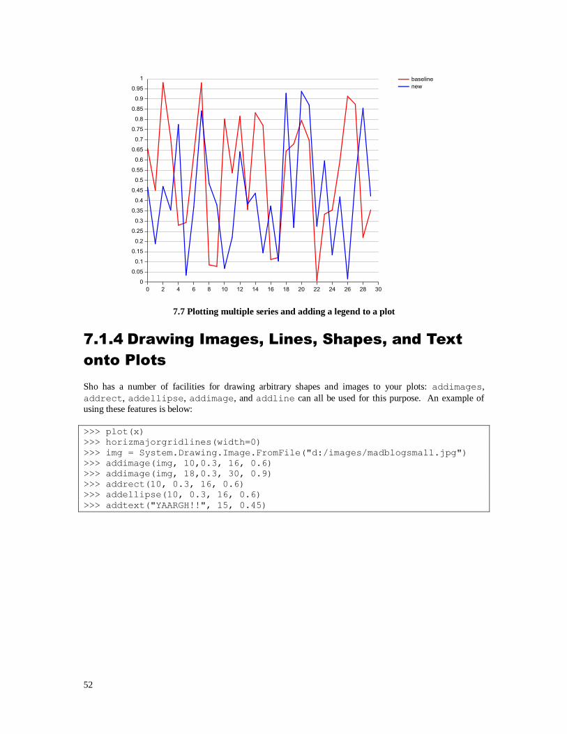
52
7.7 Plotting multiple series and adding a legend to a plot
7.1.4 Drawing Images, Lines, Shapes, and Text
onto Plots
Sho has a number of facilities for drawing arbitrary shapes and images to your plots: addimages,
addrect, addellipse, addimage, and addline can all be used for this purpose. An example of
using these features is below:
>>> plot(x)
>>> horizmajorgridlines(width=0)
>>> img = System.Drawing.Image.FromFile("d:/images/madblogsmall.jpg")
>>> addimage(img, 10,0.3, 16, 0.6)
>>> addimage(img, 18,0.3, 30, 0.9)
>>> addrect(10, 0.3, 16, 0.6)
>>> addellipse(10, 0.3, 16, 0.6)
>>> addtext("YAARGH!!", 15, 0.45)
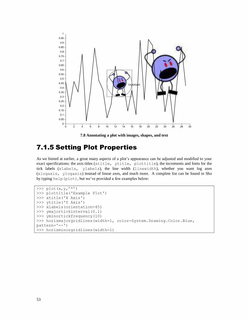
53
7.8 Annotating a plot with images, shapes, and text
7.1.5 Setting Plot Properties
As we hinted at earlier, a great many aspects of a plot‟s appearance can be adjusted and modified to your
exact specifications: the axis titles (xtitle, ytitle, plottitle), the increments and fonts for the
tick labels (xlabels, ylabels), the line width (linewidth), whether you want log axes
(xlogaxis, ylogaxis) instead of linear axes, and much more. A complete list can be found in Sho
by typing help(plot), but we‟ve provided a few examples below:
>>> plot(x,y,‟*‟)
>>> plottitle('Example Plot')
>>> xtitle('X Axis')
>>> ytitle('Y Axis')
>>> xlabels(orientation=45)
>>> ymajortickinterval(0.1)
>>> yminortickfrequency(10)
>>> horizmajorgridlines(width=1, color=System.Drawing.Color.Blue,
pattern='--')
>>> horizminorgridlines(width=1)
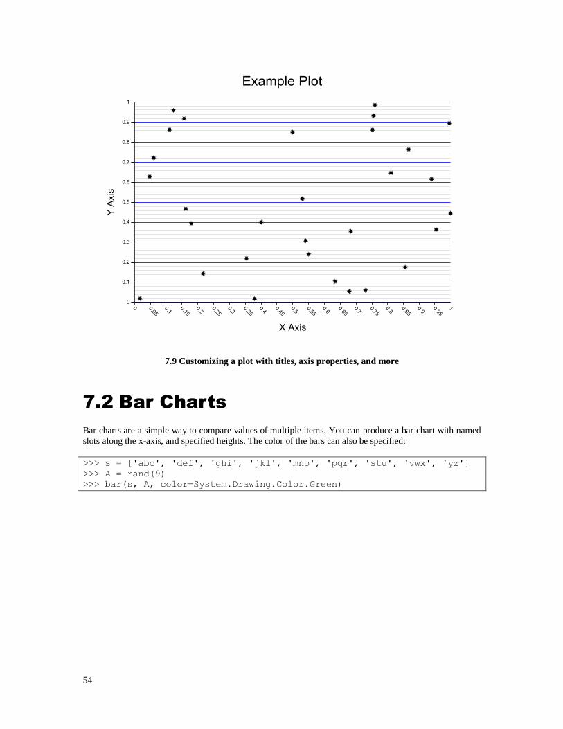
54
7.9 Customizing a plot with titles, axis properties, and more
7.2 Bar Charts
Bar charts are a simple way to compare values of multiple items. You can produce a bar chart with named
slots along the x-axis, and specified heights. The color of the bars can also be specified:
>>> s = ['abc', 'def', 'ghi', 'jkl', 'mno', 'pqr', 'stu', 'vwx', 'yz']
>>> A = rand(9)
>>> bar(s, A, color=System.Drawing.Color.Green)

55
7.10 A basic bar chart using the bar command
You can also plot multiple series on the same bar chart with custom colors and a legend:
>>> categories = ['user1', 'user2', 'user3', 'robot']
>>> trial1scores = [1.7, 2.3, 1.8, 5.0]
>>> trial2scores = [2.2, 1.9, 1.9, 4.8]
>>> bar(categories, trial1scores, 'b', categories, trial2scores, 'r')
>>> legend('trial 1', 'trial 2')
7.11 A bar chart with multiple series and a legend

56
7.3 DataGridView
If you want to look at the values of your 2D data in an editable grid, you can use the datagrid view, through
the dgv function:
>>> d = rand(20, 30)
>>> dgv(d)
This produces a data grid view in a separate window, with scroll bars:
7.12 Viewing and editing tabular data with the dgv command
There are a number of optional keyword arguments you can give to dgv in order to customize the way the
data is displayed. For instance, you can use the color keyword to have the cells colored according to their
value, and set the width of each cell to form a more image-like array:
>>> d = DoubleArray.From(drange(0, 1, 0.05))
>>> dgv(d.T*d, color=True, colWidth = 30)

57
Figure 7.13 Using cell coloring with dgv
When you put the data grid view into a variable, you can modify its properties after displaying it. So, we
could achieve the same display as above with this sequence:
>>> g = dgv(d)
>>> g.colorize()
>>> g.setColWidth(30)
The colorization automatically finds the largest and smallest entries of your 2D data. It can also take
minVal and maxVal keyword arguments to override those automatic values. Note also that dgv can take
multiple data arguments – it treats each argument as a column of data, they needn‟t be the same type or
have the same length.
In fact, dgv remembers the arguments you pass to it, and if they are mutable objects, it is possible to edit
their values from the data grid view. To toggle between edit and read-only modes, you can hit the F2 key
(alternately, you can make the view come up in edit mode by setting the keyword parameter edit to
True, and you can disable toggling edit mode by setting the keyword parameter locked to True). If the
collection you are displaying is a typed collection (an IntArray, for instance), dgv will try to coerce the
text you type into the cell into a legal value for that collection. Otherwise, it will set that entry to be the string you typed in.
If the values in the collection you‟ve displayed with dgv change, you can hit F5 to refresh the view to
reflect the new values.

58
7.4 Contour Plots
The contour function draws isovalue curves on 2D data so that you can easily get a sense of the
underlying topology.
>>> d = DoubleArray.From(drange(0,1,0.05))
>>> contour(d.T*d, bounds=[0.0, 0.0, 1.0, 1.0])
Figure 7.14 Creating a contour plot with the contour function
7.5 Viewing Arrays as Images
Another way to visualize arrays is to treat them as images and apply a colormap to them to represent the
range of values. The Sho function imageview provides a way to do this:
>>> v = DoubleArray.From(sin(drange(0, PI, 0.1)))
>>> imageview(v.T*v)

59
Figure 7.15: Viewing an array as an image with imageview
By default, the image is scaled to fill the window. Pressing „z‟ toggles between scale-to-fit mode and
manual zooming mode. In manual mode, the +/- keys zoom the image in and out, and hitting <space> sets
the zoom level so that 1 pixel represents 1 value in the underlying dataset. The „s‟ key switches between
nearest-neighbor (the default) and bilinear interpolation when zoomed in on an image.
If you want the bitmap itself, you can create it via the arrayimage function. The resulting bitmap can
then be passed to imageview in order to display it.
Of course, the imageview command can also be used directly on .NET Image and Bitmap objects:
>>> img = System.Drawing.Image.FromFile("d:/images/madblogsmall.jpg")
>>> imageview(img)
Figure 7.16 Displaying a .NET
Image with imageview

60
7.6 Interactive Histograms
Sho has a histogram plot control, which combines the bar chart plot with the Histogram class. A nice feature about the histogram plot control is that it provides a slider for changing the number of bins.
>>> a = randn(1000)
>>> hist(a)
7.17 Displaying interactive histograms with the hist command
Note that hist and Histogram both take the same optional arguments – hist simply passes its
arguments along to Histogram.
7.7 Inline plots in ShoConsole
The Sho Console also allows you to quickly view a plot (or other graphical object) inline. This can be done
using the show, showplot and showbar commands:

61
7.18 Displaying inline plots in the Sho Console with the show command
7.8 Copying, Exporting, and Saving
Plots
If you want to include Sho plots inside a document, you have a number of options. If you just want to
insert your plots into Word or an email, the easiest path is to use copy and paste: just click on a plot
window, hit Ctrl-C, and then hit Ctrl-V in your application. This will create a vector (scalable) image where
possible (e.g., in Word), and otherwise a bitmap (e.g., in Powerpoint, Outlook, Paint, etc.).
You can also save them to disk in a number of formats, including .gif, .jpg, .tif, .png (image formats) or
.emf and .eps (vector formats) with the saveplot function:
>>> saveplot("myplot.emf") # vector format
>>> saveplot("myplot.jpg") # image format

62
Chapter 8: .NET
This chapter will show you how to connect to the vast world of .NET libraries and utilities from Sho.
Fortunately, this is very easy, again due to the power of IronPython – all .NET objects are first class objects
in IronPython, and you can freely access them. In the following sections, we will show you how to load and
use existing .NET libraries.
8.1 Using .NET Framework Classes
Most framework libraries are already loaded into Sho for you, so all you have to do is import the
namespace. For instance, to use the System.IO namespace,
>>> import System.IO
>>> f = System.IO.FileInfo("c:/tmp/sho.wav")
If you want to use the items from the namespace without fully qualifying the names, you can use the
“from namespace import symbol” syntax. To get all the symbols from a namespace, you can
replace symbol with *:
>>> from System.IO import *
>>> f = FileInfo("c:/tmp/sho.wav")
There are other namespaces that are not loaded into Sho by default but are still part of the .NET framework.
For these, you‟ll have to use clr.AddReference before importing the namespace:
>>> clr.AddReference("System.Xml")
>>> from System.Xml import *
8.2 Using Other .NET Libraries
Using an existing assembly (managed DLL) in Sho is a two-step process. First, you need to load the
assembly into the Sho process, then import the primary namespace from the assembly. Let‟s say you have a library mylib.dll implementing namespace mylib in c:/tmp. Here‟s how you would load it:
>>> ShoLoadAssembly("c:/tmp/mylib.dll")
>>> import mylib
Note that this method should only be used for assemblies that you are not planning to modify during your
Sho session. In a later chapter, “Extending Sho,” we will show how you can update/rebuild your libraries
and dynamically update the behavior of your classes inside Sho.

63
8.3 Using COM Libraries
Fortunately, .NET has provided a simple mechanism for converting COM libraries to .NET assemblies, assuming the COM library exposes a type library (most do). The command you need for this is tlbimp,
which can be found in your Windows SDK directory, e.g., C:\Program Files\Microsoft
SDKs\Windows\v6.0A\Bin\TlbImp.exe. The name of the resulting assembly will match the name
of its primary namespace. The example below shows how to convert the COM .dll that comes with SAPI to
a .NET assembly. From a command prompt, first do:
C:\Program Files\Common Files\Microsoft Shared\Speech> tlbimp sapi.dll
This creates SpeechLib.dll, a .NET assembly, in that directory. Then from Sho,
>>> addpath("c:/Program Files/Common Files/Microsoft Shared/Speech/Spee
chLib.dll")
>>> ShoLoadAssembly("c:/Program Files/Common Files/Microsoft Shared/Spe
ech/SpeechLib.dll")
>>> import SpeechLib

64
Chapter 9: Extending Sho
There are many ways to extend Sho with your own modules, from modules written entirely in Python to
.NET assemblies and Sho packages. This chapter will cover the various ways in which you can add your
code to the Sho environment.
9.1 Python Modules
To create a pure Python module, all you have to do is make a .py file. Let‟s look at an example, test.py:
#test.py
a = "hello"
class myclass:
def __init__(self):
self.count = 0
def increment(self,incr=1):
self.count += incr
return(self.count)
To use this file, we just import it (after including the path with addpath if necessary):
>>> import test
>>> test.a
'hello'
>>> c = test.myclass()
>>> c.increment(2)
2
Notice that all the definitions live inside the module‟s namespace, which is the same as the filename root
(test). Remember that if you want to edit test.py and then update its behavior, you‟ll have to use
reload(test) instead of import – a second import will have no effect.
One of the great things about IronPython (and thus Sho) is that .NET objects are first-class IronPython
objects. This means, for instance, that you can derive your Python classes from .NET classes. This can be
particularly useful when creating new WinForms widgets or implementing interfaces. To do this, simply
use the .NET class name in the parent class slot:
class myclass(System.Windows.Form):
...
9.2 Single C# Files
If you want to implement some functionality in C# but it would fit easily into a single C# file and you don‟t
want to make an entire project around it, we‟ve made an easy way to do this via the load command.
Here‟s a simple example (which you can find in the {SHODIR}\playpen directory):

65
// addstuff.cs
namespace AddStuff {
public class MyAdder {
public int hello() {
System.Console.Out.Write("foo\n");
return 43;
}
}
}
To use this, load the .cs file and then import the namespace. The load command will invoke the C#
compiler and load the assembly.
>>> load("addstuff.cs")
csc.exe /target:library
/out:"C:\Users\sumitb\AppData\Local\Temp\sho_tmp58CTBLSGBU5HREJAU9O0233
F4\addstuff_3ZCZ74AL069ZLZMRJ4WGTH85D.dll" /debug
"c:\src\sho2\Sho\Current\playpen\addstuff.cs"
Microsoft (R) Visual C# 2005 Compiler version 8.00.50727.4927
>>> import addstuff
>>> m = addstuff.MyAdder()
>>> m.hello()
42
If you have additional arguments you need to give the compiler, you can fully specify the command line via
a comment line at the top of the file that starts with cscargs:. In the example below, matrixexample.cs
(also in {SHODIR}\playpen), we create a C# file which will horizontally flip a DoubleArray. Since it
takes and returns DoubleArrays, we need to reference the appropriate assemblies:
// matrixexample.cs
//
// cscargs: /r:"{SHODIR}\bin\MatrixInterf.dll" \
/r:"{SHODIR}\bin\ShoArray.dll" /debug /target:library
using ShoNS.Array;
namespace matrixexample
{
public class tester
{
public DoubleArray fliphoriz(DoubleArray d)
{
DoubleArray e = new DoubleArray(d.Size[0],d.Size[1]);
for (int i = 0; i < d.Size[0]; i++) {
for (int j = 0; j < d.Size[1]; j++) {
e[i,j] = d[i,d.Size[1]-1-j];
}
}
return(e);
}
}
}

66
Note that the {VARNAME} notation expands environment variables; in the example above SHODIR is set
to c:\Program Files\Sho. We can now load this just like the previous C# file:
>>> load("matrixexample.cs")
>>> import matrixexample
>>> t = matrixexample.tester()
>>> t.fliphoriz(DoubleArray.From([1,2,3,4,5]))
[5.0000 4.0000 3.0000 2.0000 1.0000]
Note that we can now update testmatrix.cs to change its behavior and load it again; new instances of
testmatrix.tester will then reflect the new behavior.
9.3 Dynamically Extending Sho with
Visual Studio
If you have more complex libraries to build, wish to use a different .NET language (such as C++/CLI or
VB .NET), or are simply more comfortable in the Studio environment, but still want to interactively update
and reload your libraries inside Sho, it is straightforward to do so with Visual Studio. There are a few small
things to keep in mind, though, and we detail them below.
9.3.1 Signing the Assembly
In order for .NET to pay attention to the version number when reloading a .dll, it needs to be strongly-named, which means you need to sign it. This is easy to do from inside Studio: simply go to the Properties
page for your C# project (right click on the project name and choose properties), then select the Signing tab
as shown below.
Figure 9.1: Setting up Strong Naming (aka Assembly Signing) in the Properties pane of a C# project

67
Turn on the check mark for “Sign the Assembly,” and then select <New> under the “Choose a strong name
key file” drop down. You‟ll have the option of choosing a password to protect your keyfile, which you
most likely don‟t need.
9.3.2 Auto-Updating the Assembly Version
The next step is to make sure Visual Studio auto-updates the assembly version number every time you
build. In the file explorer for the project, open up the Properties folder to reveal AssemblyInfo.cs and open that file. The bottom part of the file will look something like this:
// Version information for an assembly consists of the following four
values:
//
// Major Version
// Minor Version
// Build Number
// Revision
//
// You can specify all the values or you can default the Revision and
Build Numbers
// by using the '*' as shown below:
[assembly: AssemblyVersion("1.0.0.*")]
[assembly: AssemblyFileVersion("1.0.0.0")]
The key is to make the AssemblyVersion end with a “*” as you see above. Unfortunately, the default is
“1.0.0.0”, which will result in the version number being fixed, so you will have to edit this.
9.3.3 Loading/Reloading the Assembly from Sho
Since we‟re going to be updating this assembly, we want to make sure not to lock the file. To do this, we‟ll
use the load command again, this time on the .dll:
>>> addpath("c:/src/CSharpLibraryExample/bin/Debug")
>>> load("CSharpLibraryExample.dll")
>>> import CSharpLibraryExample
>>> c = CSharpLibraryExample.Class1()
>>> c.message
""
Note that instead of the addpath command, we could also have specified the full path for load. Again,
note that we need to load the assembly and then import the namespace.
When we want to update the code/assembly and reload it, we first rebuild the assembly from Visual Studio,
and then load it back into Sho:
# update C# file in Visual Studio so c.message is “hello world”
# and rebuild the dll
>>> load("CSharpLibraryExample.dll")
>>> c = CSharpLibraryExample.Class1()
>>> c.message
"hello world"

68
Note that we didn‟t have to re-import the namespace, but we did have to re-load the new assembly, as well
as re-instantiate the variables; this resulted in the new behavior of the class. If we didn‟t reinstantiate c, it
would still have its old behavior – in fact, the old dll is still attached to the process, and we could even have
“saved” its namespace by setting CSharpLibraryExample_old = CSharpLibraryExample
before re-loading.
9.3.4 Debugging the Assembly
Debugging your assembly in this scenario is fairly straightforward as well. Simply set a breakpoint in your
code, and then click on Debug->Attach to Process in Visual Studio. You‟ll see a list of processes; select
“shoconsole.exe” if you‟re using the Sho console, and “shopy.exe” if you‟re using the command
shell console. The break point will become a red outline for a second, but then will become a filled in red
dot again. Once it‟s refilled, you can execute code from Sho and break in the C# code inside Studio,
examine variables, the call stack, etc.
Figure 9.2: Debugging a C# project while it's being called from Sho
9.4 Sho Packages
The official method for supplementing Sho‟s functionality in a way that you can share with others is via
Sho packages. Sho packages are simply a way to gather together a file or set of files that implement some
coherent functionality, and to expose the proper pieces in the top-level Sho namespace. A package consists
of a directory named packagename in {SHODIR}/packages (defined in the Sho variable
shopackagedir), and at the least, a Python file inside that directory named __init__.py . You can
tell Sho to import a subset of the content of your package into the global namespace by setting the
sho_import_list variable inside __init__.py. Here is an example of a simple package file that
defines a variable, two functions and a class, and exports everything except one of the functions into the
global namespace:
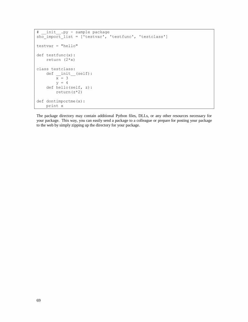
69
# __init__.py - sample package
sho_import_list = ['testvar', 'testfunc', 'testclass']
testvar = "hello"
def testfunc(x):
return (2*x)
class testclass:
def __init__(self):
x = 3
y = 4
def hello(self, z):
return(z*2)
def dontimportme(x):
print x
The package directory may contain additional Python files, DLLs, or any other resources necessary for
your package. This way, you can easily send a package to a colleague or prepare for posting your package
to the web by simply zipping up the directory for your package.

70
Chapter 10: Using Sho
from .NET
Many times you will want to use Sho code in your own C# programs. This chapter describes how to use the
Sho library code (array and visualizations) as well as your own (Python-based) Sho code.
10.1 Writing .NET Code Using Sho
Libraries
While most of the user interface/utility libraries in Sho are written in IronPython, the core math (array) and
plotting libraries are written in C#. If you wish to use these libraries in your own programs or in libraries
that extend Sho, you‟ll have to reference the appropriate libraries. We list the common cases below.
If you want to use Sho Arrays, see the example in the earlier section, “Single C# Files,” for how to use the library from .NET. If you‟re just using the array library, make sure to add the following references:
1. {SHODIR}\bin\ShoArray.dll
2. {SHODIR}\bin\MatrixInterf.dll
3. [optional] {SHODIR}\bin\MathFunc.dll
4. [optional] {SHODIR}\bin\ShoViz.dll
The classes in the first two DLLs implement the ShoNS.Array namespace and are necessary for any
program or library that will call the Sho libraries. The third DLL, Mathfunc.dll, implements the
ShoNS.MathFunc namespace, which is handy to have if you‟re doing any mathematical manipulations
in your code. The fourth entry, ShoViz.dll, implements the ShoNS.Visualization namespace, and is
required if you‟re going to call any of Sho‟s plotting or visualization functions.
The figure below shows how these references will look in Visual Studio; an example project calling Sho
libraries from C# can be found in the {SHODIR}/playpen directory. Finally, since Sho 2.0 is built on .NET
4.0, your application will need to target the .NET framework 4.0. You can select this version on the
application properties page.

71
Figure 10.1: Using the Sho libraries from C# in Visual Studio
10.2 Calling Python Code from .NET
Sometimes you need to call routines you‟re developing in Sho from a .NET program. For instance, perhaps
you‟ve been working on a clustering algorithm in Sho, and are working with a team that has a C#
application that wants to use your clustering algorithm. It turns out you can do this via the EmbeddedSho
class, available in EmbeddedSho.dll. This class takes a pointer to a Sho directory and creates a private
instance of Sho in which you can create Sho variables pointed to objects from your application, call
methods, get return values, make plots, etc.
To use it, you need to add references to EmbeddedSho.dll, IronPython.dll, and
IronPython.dll (all in shobindir). The API is best explained by the C# example below:

72
static void Main(string[] args)
{
// create the Embedded Sho
System.Console.Write("Starting Embedded Sho...");
// the path argument below should point to what "SHODIR" evaluates
// to in Sho
EmbeddedSho es = new EmbeddedSho("c:/src/sho2/sho/current");
System.Console.Write("done.\n");
// es.CacheShoOutput will store the output from Sho so you can show
// it in a form, etc;
// if you don't call this the default is to print the output to
//the console.
es.CacheShoOutput();
// create a class from the containing assembly
TestClass t = new TestClass();
// put it into the Sho environment
es.SetPythonVariable("tc", t);
// do some Sho stuff
es.ExecutePython("a = rand(10,10)");
es.ExecutePython("foo = a[0,0]");
// print information from the class
es.ExecutePython("print tc.info");
// print cached output from Sho
System.Console.WriteLine("{0}", es.GetOutputText());
es.ExecutePython("plot([1,2,3,4,5])");
// get the result in res so we can bring it back to C#
es.ExecutePython("res = tc.info");
es.ExecutePython("for x in range(10): print x");
// print cached output text. This can be called as often as
//you wish; the text is flushed each time.
System.Console.WriteLine("{0}", es.GetOutputText());
// get back and print Sho values
// note that GetPythonVariable will return an Object, which we
//can cast to a known type
System.Console.WriteLine("foo: {0}", es.GetPythonVariable("foo"));
// alternatively, we can use GetPythonVariableAs<type>, which
//will cast it to the type in one call.
System.Console.WriteLine("res: {0}",
es.GetPythonVariableAs<String>("res"));
}
An example project showing how to call Sho code from C# can be found in the {SHODIR}\playpen
directory.
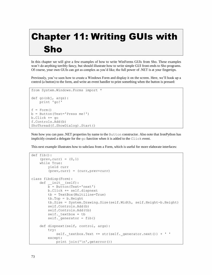
73
Chapter 11: Writing GUIs with
Sho
In this chapter we will give a few examples of how to write WinForms GUIs from Sho. These examples
won‟t do anything terribly fancy, but should illustrate how to write simple GUI front-ends to Sho programs.
Of course, your own GUIs can get as complex as you‟d like; the full power of .NET is at your fingertips.
Previously, you‟ve seen how to create a Windows Form and display it on the screen. Here, we‟ll hook up a
control (a button) to the form, and write an event handler to print something when the button is pressed:
from System.Windows.Forms import *
def go(obj, args):
print 'go!'
f = Form()
b = Button(Text='Press me!')
b.Click += go
f.Controls.Add(b)
ShoThread(f.ShowDialog).Start()
Note how you can pass .NET properties by name to the Button constructor. Also note that IronPython has
implicitly created a delegate for the go function when it is added to the Click event.
This next example illustrates how to subclass from a Form, which is useful for more elaborate interfaces:
def fib():
(prev,curr) = (0,1)
while True:
yield curr
(prev,curr) = (curr,prev+curr)
class fibdisp(Form):
def __init__(self):
b = Button(Text='next')
b.Click += self.dispnext
tb = TextBox(Multiline=True)
tb.Top = b.Height
tb.Size = System.Drawing.Size(self.Width, self.Height-b.Height)
self.Controls.Add(b)
self.Controls.Add(tb)
self._textbox = tb
self._generator = fib()
def dispnext(self, control, args):
try:
self._textbox.Text += str(self._generator.next()) + ' '
except:
print join('\n',geterror())

74
(Note the try/except around the Click handler function: this is to make sure that the user never gets a pop-
up error message.) Now we can create a fibdisp form and put it in its own thread:
>>> f = fibdisp()
>>> t = ShoThread(f.ShowDialog)
>>> t.Start()
Which will produce the window below. It‟s very easy to make a simple GUI to display the output of some
Python script (or other piece of code) this way.
Figure 11.1 Creating a simple GUI in Sho
Note that while some Forms functionality, like setting the text of the textbox, can be called from the
console thread (as opposed to the thread that the form is running on), other functionality, like adding
widgets, need to be invoked on the Form‟s thread. For instance, if we just tried to add a Button to the form,
we‟d see an error:
>>> b = Button()
>>> f.Controls.Add(b)
Error: Controls created on one thread cannot be parented to a control
on a different thread.
To do this properly, we‟ll need to use the Form‟s Invoke method and pass it a delegate for a function that
will add the button; this will execute the function in the context of the Form‟s thread. To create a delegate,
we‟ll use the System.Action class (if our function returned a value we‟d use System.Func instead).
>>> def foo():
f.Controls.Add(b)
>>> f.Invoke(System.Action(foo))
Since this is such a common task, we‟ve created a couple of convenience functions in Sho to make it easier:
>>> AddControl(f, b) # add the button to form f
>>> RemoveControl(f, b) # ...and then remove it
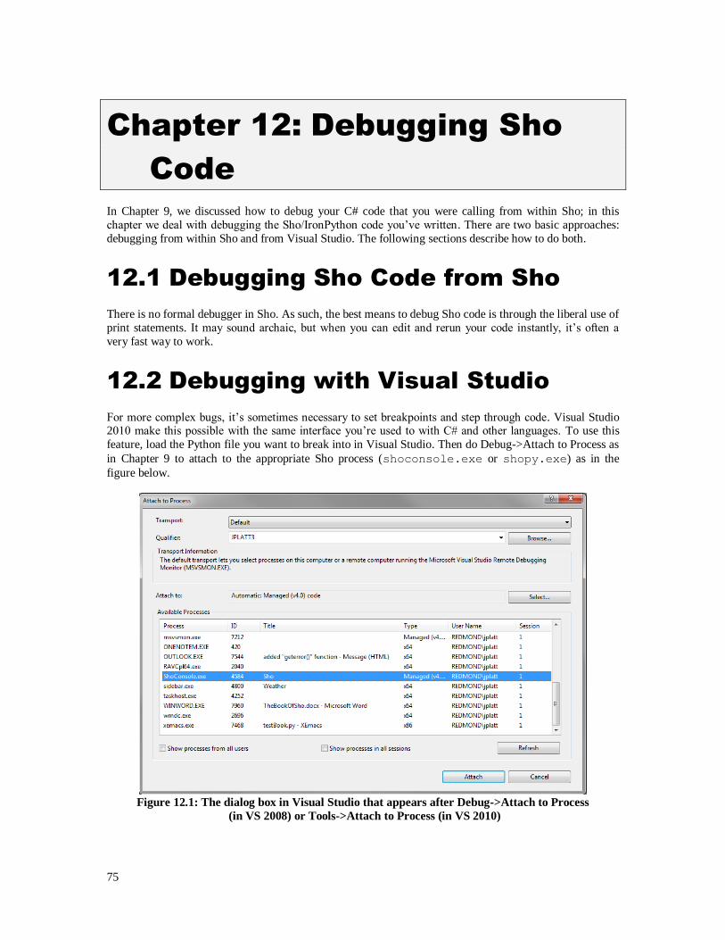
75
Chapter 12: Debugging Sho
Code
In Chapter 9, we discussed how to debug your C# code that you were calling from within Sho; in this
chapter we deal with debugging the Sho/IronPython code you‟ve written. There are two basic approaches:
debugging from within Sho and from Visual Studio. The following sections describe how to do both.
12.1 Debugging Sho Code from Sho
There is no formal debugger in Sho. As such, the best means to debug Sho code is through the liberal use of
print statements. It may sound archaic, but when you can edit and rerun your code instantly, it‟s often a
very fast way to work.
12.2 Debugging with Visual Studio
For more complex bugs, it‟s sometimes necessary to set breakpoints and step through code. Visual Studio 2010 make this possible with the same interface you‟re used to with C# and other languages. To use this
feature, load the Python file you want to break into in Visual Studio. Then do Debug->Attach to Process as
in Chapter 9 to attach to the appropriate Sho process (shoconsole.exe or shopy.exe) as in the
figure below.
Figure 12.1: The dialog box in Visual Studio that appears after Debug->Attach to Process
(in VS 2008) or Tools->Attach to Process (in VS 2010)

76
You can import the Python file into the Sho process before or after this point. If you set breakpoints in your
Python code (or your C# code called from Python), the debugger will stop there as shown in the figure
below. You can then step through the code, step into and over functions, examine local variables, etc.
Figure 12.2: Stopping at a breakpoint in Python code in Visual Studio
77
Chapter 13: Epilogue
Like any good guidebook, we‟ll leave you with a few tidbits that may be helpful in your journey. We‟ll
take this opportunity to point you to a few resources you can use to learn more about Sho, and then send
you off into the world of code.
13.1 Other Resources
In addition to this book and the self-documentation tools inside Sho, there are a few other resources we recommend if you‟re ready to get into some serious Sho hacking.
The Sho Blog. (http://blogs.msdn.com/b/the_blog_of_sho/) This is a starting point for all things
Sho: from there you can get the latest installer, find the latest packages, and see screenshots and
videos of Sho in action.
IronPython and Python Books. While this book has given you a brief overview of the
IronPython language, it‟s handy to have a book about it on hand. For the experienced Python
programmer, Michael Foord and Christian Muirhead‟s IronPython In Action (Manning) is a great
guide to the language; it‟s the first book specific to IronPython and has received great reviews.
For Python beginners, Mark Lutz and David Ascher‟s Learning Python (O‟Reilly) is a fantastic
introductory guide to the very powerful Python language.
IronPython Sites. There are a variety of resources on the web for Python, but the “IronPython Cookbook” (http://ironPython.info) has some great examples of how to do cool things (Silverlight,
Interop, XML) in IronPython.
C# Books. If you‟re going to be doing serious work in Sho, you‟ll likely be writing some C# or
C++/CLI code. We found Jesse Liberty‟s Learning C# (O‟Reilly) to be excellent not only for
getting into C#, but learning a lot about all the goodies in .NET.
.NET Books. One of the great things about Sho (because of IronPython) is that all of .NET is
immediately accessible to you. To find out more about how to do basic things, we highly
recommend Charles Petzold‟s Programming Windows in C# (Microsoft Press). This is very
similar to his extremely popular Programming Windows, but this time for managed code. We
affectionately refer to it as “Petzold dot NET.”
Reporting Bugs. If you encounter any bugs, please send them to the Sho Feedback mailing list ([email protected]).
13.2 And You’re Off!
That‟s all we have to tell you for now - we hope you enjoy the Sho environment and that it becomes useful
to you in your own work. Hopefully, you‟ll soon have something to tell us too! Sho is for you, the users,
and we would love to get your feedback about your experiences with it. We welcome your comments at
[email protected]. Have fun with Sho, and we look forward to hearing from you!


