THE ZEEMAN EFFECT 190529

Introduction

Quantum mechanics tells us that angular momenta, J , are quantized both regarding

magnitude, 2 2 ( 1)J J J , and direction, z JJ M , as illustrated in Figure 1. The

directional quantization is normally not noticeable in the energy level structure of an

atom since the "z"-direction is an arbitrary

direction (isotropic space), and all states that

differ only in the value of MJ have the same

energy. The level is said to be 2J + 1 fold

degenerate. However, if the atom is placed in an

external magnetic field the degeneracy is broken

due to energy differences between states that are

aligned with the external field and states that are

not. Thus, the different MJ - states obtain a small

additional energy:

mag J B JE g BM .

Here gJ is the Landé factor for the level, μ𝐵is the

Bohr magneton, B is the magnetic field strength

and M𝐽 is the secondary total angular momentum

quantum number. Furthermore, light emitted

from an excited atom becomes polarized with an

oscillation mode that depends on how the MJ

quantum numbers change as well as the direction

of observation relative to the external magnetic

field. Viewed perpendicular to the B-field light is

linearly polarized; oscillating parallel to the field for ∆MJ = 0 transitions and

perpendicular for ∆MJ = ±1. Viewed along the field direction ∆MJ = ±1 transitions give

rise to circularly polarized light.

Preparation

Study carefully the theory of the Zeeman effect in e.g. Thorne et al, Spectrophysics1, Ch.

3.9.1 or Foot, Atomic Physics2, Ch. 1.8 and 5.5. Since the Zeeman splitting of spectral

lines is small, we need an instrument with very high spectral resolution to measure it.

One such instrument is the Fabry-Perot interferometer described in Spectrophysics 13.1

- 13.4, Pedrotti et al, Introduction to Optics3 and also briefly in Appendix 1, below. You

must study in detail (at least) the last section of Appendix 1, where the evaluation of the

experiment is described. Recapitulate the description, production and manipulation of

polarized light. This is very briefly outlined in Appendix 2. If you are not familiar with

the concept of polarization, read the section “Linear Polarization” on p. 1115 of

University Physics with Modern Physics and “Circular and Elliptical Polarization” on p.

1121 in the same book (e-book available through the physics library at

https://lubcat.lub.lu.se/).

1 A. Thorn, U. Litzén and Se. Johansson, Spectrophysics, Springer 2 C. Foot, Atomic Physics, Oxford master series in Physics 3 F.L. Pedrotti, L.M. Pedrotti and L.S. Pedrotti, Introduction to Optics, Pearson 4 H.D. Young, R.A. Freedman, A.L. Ford, University Physics with Modern Physics, Global ed., Pearson

Preparatory exercises (Serious attempts must be made on all exercises)

1. The ground configuration in neutral Cd is 5s2 and the first excited configuration is

5s5p. In the experiment you will, among other lines, see the transition

5s5p 3P - 5s6s 3S.

a) Give the LS notation for the possible transitions between these terms.

b) You will find a green ( = 508.582 nm), a turquoise ( = 479.992 nm) and a

blue ( = 467.816 nm) line. Which of the transitions above correspond to the

different colors?

2. This exercise is essential to the lab and a solution must be presented before you

are allowed to continue.

In the experiment you will study the transitions 5s5p 1P1 - 5s5d 1D2,

5s5p 3P2 - 5s6s 3S1, 5s5p 3P1 - 5s6s 3S1 and 5s5p 3P0 - 5s6s 3S1 in a weak magnetic

field.

a) Derive the Landé g factor assuming LS coupling for the levels involved in the

four transitions.

b) Draw large and nice diagrams showing the different Zeeman components that

each of the 4 lines (not levels) split into in the magnetic field in the manner of

Figure 3.16 in Spectrophysics or Figure 5.13 in Atomic Physics. Thus, choose

a relative energy scale, with zero at the energy of the transition without

magnetic field, and show the splittings in units of µBB along the x – axis. Let

all Zeeman components have the same intensity.

c) What is the state of polarization of each of the components? (Hint: ΔM is

positive if MJ of the upper state > MJ of the lower state)

d) Which components do you expect to see in a direction parallel to the magnetic

field?

3. Let B = 0.5 T. How large is the smallest splitting between the components derived

above?

a) Expressed in eV

b) Expressed in cm-1

c) Expressed in nm

4. Use Appendix 1 to answer the following. A Fabry-Perot interferometer operating

in air have mirror surfaces with a reflectance of R = 0.85 and separated by

3.085 mm. We use a light source with a wavelength of 500 nm.

a) What is the free spectral range expressed in cm-1 and in nm.

b) What is the line width expressed in cm-1 and nm.

c) Does the size of the rings increase or decrease in higher spectral orders?

5. Use Appendix 2 to answer the following. What is the polarization of light when the

electric field is described by the expressions below?

a) ))cos()sin((0 tkzetkzeEE yx

b) )sin(3)2/sin(5 tkzetkzeE yx

Experiments

Setup

Neutral cadmium atoms have the ground configuration 5s2 and the system of excited

levels 5snℓ. In the experiment you are going to study the 4 lines

5s5p 1P1 - 5s5d 1D2 643.8 nm (red)

5s5p 3P2 - 5s6s 3S1 508.6 nm (green)

5s5p 3P1 - 5s6s 3S1 480.0 nm (turquoise)

5s5p 3P0 - 5s6s 3S1 467.8 nm (blue)

The cadmium light is emitted from a spectral lamp placed between the poles of an

electromagnet, where the field is directly proportional to the current. Light then passes

through a Fabry-Perot interferometer and the interference pattern is studied either by eye

or with a CCD camera. The setup is shown in Figure 2. The lenses have focal lengths of

50, 300 and 50 mm as indicated in the figure.

To isolate a certain wavelength from the Cd-

light (to look at one transition at the time) we

need external narrow band interference filters.

Figure 3 shows the transmission curves for the

filters for the blue and the turquoise light.

The polarization of the Zeeman components of

light emitted perpendicularly and parallel to the

magnetic field is investigated using a polarizer

and an achromatic λ/4 plate (see Appendix 2).

Qualitative studies (the most important part!)

Start by viewing the Fabry-Perot interference patterns

directly by putting your eye immediately behind the

last lens. Optimize the positions of the lenses to see

the pattern as clearly as possible. What happens when

you use different filters or different magnetic field

strengths? Study the transitions from both the

transverse and longitudinal direction with regards to

the magnetic field. Do your observations agree with

the predictions in preparatory exercise 2? Is

something missing in one direction and in that case

why? Then, insert the polarizer and other necessary

[Gra

b

your

reade

r’s

attent

ion

with

a

great

quote

from

the

docu

ment

or

use

this

space

to

emph

asize

a key

point

. To

place

this

text

box

anyw

here

on

the

page,

Figure 3. Transmission curves for the

interference filters used. Data from

Thorlabs, http://www.thorlabs.com/.

f = 50

Figure 2. The experimental setup.

CCD-Camera

f = 300 f = 50

Figure 4. Fabry-Perot pattern with

no filters or magnetic field.

instruments and verify the polarization of the σ-components you determined in exercise

2.

Quantitative studies

Carefully adjust and center the CCD camera on the pattern. The software uEye Cockpit

allows you to capture images with the camera. The brightness can be adjusted by tuning

certain camera parameters (for example the exposure time) that you can find through:

tool → camera.

Perform a set of measurements in the direction that gives you the clearest image of the

σ - splittings, for each transition. If you use the transverse direction, you need to use one

additional optical instrument. Take data for several magnetic currents between 0 and, at

most, 4A (NOTE! For one of the setups the maximum is 3A) and capture the ring pattern

for each setting to a file. You will need several points in

order to perform the fitting, so do not take too few values

for the magnetic current!

As a preparation for the quantitative analysis according

to eq. (7) in Appendix 1, use the software Motic Images

Plus, load an image, then go to the "Measurements"

menu and choose the "3-point circle" to determine the

diameter of the observed rings for each magnetic current,

as illustrated in Figure 5. Make sure to save these images

to a USB-stick for the analysis and the report writing!

Use eq. (7) in Appendix 1 and your measured diameters

and plot, in the same diagram, the Zeeman splitting, ∆σ,

as a function of the current through the magnet for the

different transitions. The magnetic field is directly proportional to the current, as shown

in Figure 6 for currents up to 5 A. Verify that the Zeeman splitting is, indeed, directly

proportional to the magnetic field. To compare the numerical value of the splittings to

the theoretical prediction you need the approximate proportionality constants which are

0.1 T/A for the Phywe magnets and 0.058 T/A for the "large magnet".

a b

Figure 6. Magnetic field as a function of current for the a) Phywe magnets and

b) "Large magnet".

To eliminate also the need to accurately know the thickness of the spacer between the

plates in eq. (7), show that the ratio of the slopes of the red and blue lines is accurately

predicted by the quantum numbers and gJ - factors involved, see preparatory exercise 2.

0 5 100

0.1

0.2

0.3

0.4

0.5

Magnetic current / A

Ma

gn

etic f

ield

/ T

Figure 5. Fitting of the Fabry-

Perot rings with the 3-point-

circle tool in Motic Images Plus.

Fitting your results

Since you expect a linear relation between magnetic current and splitting, it is

recommended to use a linear fit to the data. It is allowed to use built-in functions in for

example MATLAB for this, but you can also use a manual least-squares method by trying

out different values on k and m for 𝑦 = 𝑘𝑥 + 𝑚 and see which values minimize

∑ (𝑦(𝑥𝑖)𝑚𝑒𝑎𝑠𝑢𝑟𝑒𝑑 − 𝑦(𝑥𝑖)𝑓𝑖𝑡)2𝑁𝑖 , where N is the total number of data points taken. From

this you can also find the standard deviation S:

𝑆 = √∑ (𝑦(𝑥𝑖)𝑚𝑒𝑎𝑠𝑢𝑟𝑒𝑑−𝑦(𝑥𝑖)𝑓𝑖𝑡)

2𝑖

𝑁

The value of S might be interesting to compare to your own estimation of the size of the

uncertainty in your method.

Checklists

Before you leave the lab

Before you leave the lab, make sure that you have done all of the following required

steps:

Made sure you understand the function and purpose of all instruments used.

By eye observed the effect of the longitudinal vs transverse direction of the

optical bench with regards to the magnetic field and the effect of changes in the

magnetic field strength.

Confirmed the polarization of the σ-lines and fully understand the procedure.

Taken enough data points (i.e. enough current values have been used) to measure

the Zeeman splitting of the σ-lines of all transitions, unless otherwise instructed

by the supervisor, and properly fit a function to your data.

Measured the diameters D1 and D2 for the most appropriate image as well as all

necessary Da and Db, and saved these values (preferably also all images) to a USB

stick.

Before handing in your report

When writing a report, there are some details that are often overlooked, so take a look

through the short checklist below to ensure that you have not forgotten any of these

points:

Have you answered all the questions asked in the lab manual? (these questions

are there to guide your thinking and start your analytic train of thought!)

Are your plots easy to understand and do you guide the reader through them and

point out important features etc?

Do all of your figures have figure captions that are independent enough from the

text that you would be able to interpret the figure without the text?

Do all of your facts regarding the background/theory have a correct reference to

a trustworthy source?

Appendix 1:

The Fabry-Perot interferometer, free spectral range, line width and data reduction for the Zeeman lab.

You have most likely discussed the phenomenon of interference in thin films, shown in

Figure A1-1, in some earlier course. In many cases the reflectance of the surfaces is low

and only the first two rays have a substantial impact on the output. However, if the

reflectance is high we must sum the

contribution from (very) many rays, a

phenomenon called multiple beam

interference. This is the basis for the Fabry-

Perot interferometer. A typical

interferometer is shown schematically in

Figure A1-3. Two plane glass plates with

highly reflecting surfaces facing each other

are separated by a distance d. Light from an

extended source (see Figure A1-2) pass

through the system, as in Figure A1-3. The

light is reflected many times between the

plates and at each reflection a small part is

transmitted. Each transmitted wave acquires a phase difference

of δ relative to the previous one due to the extra "round trip"

between the plates:

22 cos ,nd

(1)

where λ is the wavelength in vacuum, d the distance between

the plates separated by a medium with refractive index n and θ

is the angle to the optical axis (Figure A1-3).

Figure A1-2. An

extended light source

emits light from a

finite area, unlike a

point source.

Figure A1-3. Light path through a Fabry-Perot-interferometer.

The condition for constructive interference in point P2 is:

2 cosnd m (2)

In an extended light source all rays that are emitted at an angle of θ will contribute to the

ring pattern at the angle of θ to the optical axis. Different orders (i.e. different values of

m) will appear with different diameters, as shown in Figure A1-4a.

Figure A1-4. a) Interference pattern for a monochromatic light source. b) For a light

source with two very close wavelengths.

Transmission and the free spectral range.

The theory of multiple beam interference shows that the transmitted intensity It through

a Fabry-Perot interferometer is given by the so-called Airy function.

0 0

2

2

1( ) ,

41 sin

(1 ) 2

tI I A IR

R

(3)

where R = is the reflectance of the surfaces and is the phase difference (1).

The Airy function is illustrated in Figure A1-5,

for different values of the reflectance R. We note

both from the figure and from (3) that the

function is periodic, with a period of 2π. This

period, expressed in any parameter, is called the

free spectral range (fsr), and is an important

parameter since it represents the range over

which the interferometer is useful. For example,

two wavelengths differing by Δλfsr will be

imaged on the same ring and hence impossible

to distinguish. This is refered to as overlapping

orders.

Figure A1-5. The Airy function.

To determine the free spectral range in any parameter other than phase we simply

differentiate (1) and use Δδfsr = 2. For example, Δλfsr is obtained from

)cos(41

)(2

nd

.

With fsr 2 and

fsr

2 2 2

fsr for small angels .4 cos( ) 2 cos( ) 2

fsr

nd nd nd

(4)

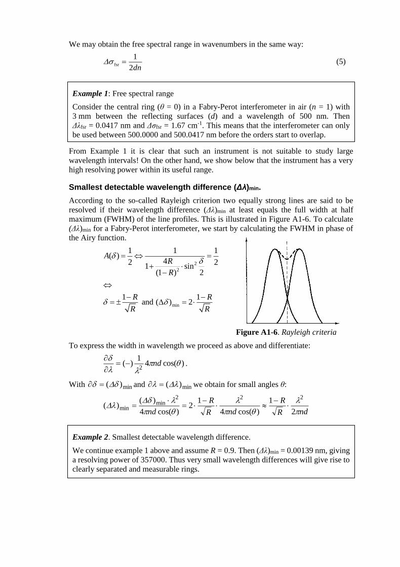
We may obtain the free spectral range in wavenumbers in the same way:

fsr

1

2dn (5)

From Example 1 it is clear that such an instrument is not suitable to study large

wavelength intervals! On the other hand, we show below that the instrument has a very

high resolving power within its useful range.

Smallest detectable wavelength difference (Δλ)min.

According to the so-called Rayleigh criterion two equally strong lines are said to be

resolved if their wavelength difference (Δλ)min at least equals the full width at half

maximum (FWHM) of the line profiles. This is illustrated in Figure A1-6. To calculate

(Δλ)min for a Fabry-Perot interferometer, we start by calculating the FWHM in phase of

the Airy function.

2

2

1 1 1( )

42 21 sin

(1 ) 2

AR

R

min

1 1 and ( ) 2

R R

R R

Figure A1-6. Rayleigh criteria

To express the width in wavelength we proceed as above and differentiate:

)cos(41

)(2

nd

.

With min)( and min)( we obtain for small angles θ:

ndR

R

ndR

R

nd

2

1

)cos(4

12

)cos(4

)()(

222min

min

Example 1: Free spectral range

Consider the central ring (θ = 0) in a Fabry-Perot interferometer in air (n = 1) with

3 mm between the reflecting surfaces (d) and a wavelength of 500 nm. Then

Δλfsr = 0.0417 nm and Δσfsr = 1.67 cm-1. This means that the interferometer can only

be used between 500.0000 and 500.0417 nm before the orders start to overlap.

Example 2. Smallest detectable wavelength difference.

We continue example 1 above and assume R = 0.9. Then (Δλ)min = 0.00139 nm, giving

a resolving power of 357000. Thus very small wavelength differences will give rise to

clearly separated and measurable rings.

Wavenumber differences from a measured Fabry-Perot ring system.

From Figure A1-3 we obtain the following relation between , the focal length f of the

lens, and the diameter D of a circle:

2 22 2 2 2 1/ 2

2 2

1cos / (1 / ) 1 1

2 8

R Df f R R f

f f

If we combine this with the condition for constructive interference (2) rewritten in terms

of wavenumber σ = 1/λ, we obtain:

2 22 (1 / 8 ) .m d D f

This expression shows that a larger ring corresponds to a smaller m, i.e. a smaller path

difference m between adjacent beams. We can estimate the magnitude of m: Suppose

we have a maximum for = 0, i.e. D = 0, and that we have d = 3 mm, which is the

distance we use in this experiment. This gives for red light ( 600 nm or

16 000 cm-1 ) m 9600.

Two adjacent spectral lines, e.g. two Zeeman components, give rise to two systems of

close lying circles, as seen in Figure A1-4b. If we want to determine the wavenumber

difference between two lines in the same interference order m with the wave numbers a

and b we get the equations:

2 2

2 2

2 (1 / 8 )

2 (1 / 8 )

a a

b b

m d D f

m d D f

We can eliminate m and d and get the equation:

2 2 2 2(1 / 8 ) (1 / 8 )a a b bD f D f (6)

Da and Db can be measured. The focal length f cannot be measured with sufficient

accuracy, but it can be eliminated in the following way. Measure the diameters of the

circles of two adjacent orders for the same line , e.g. the line we are investigating with

no magnetic field (Figure A1-3a). The two circles have the diameters D1 and D2 and the

orders m and m-1. We get the relations

2 2

1

2 2

2

2 (1 / 8 )

1 2 (1 / 8 )

m d D f

m d D f

This can be transformed into2 2 2

2 12 ( ) 8d D D f . Inserting this into (6) and using

ba gives finally

2 2

2 2

2 1

1

2

a ba b

D D

d D D

. (7)

Da and Db are in our case the diameters of the circles from two Zeeman components in a

certain order. In practice we use the highest order, i.e. the innermost circles. D1 and D2

are the diameters of two circles from the same line - with no magnetic field - in different

orders. The distance d = 3 mm for the instrument from Phywe (the same instrument that

has 3A as its maximum magnetic current) and 3.085 mm in the other interferometers.

Appendix 2 Polarized light

Light can be thought of as an electromagnetic wave consisting of an electric and a

magnetic field. The polarization describes how the electrical component of the light

behaves both in space and time. If light is polarized, it means that at a given point z both

the amplitude and the direction of the electric field vary in a regular and predictable way,

as opposed to the random variations of unpolarized light.

The superposition principle gives us a convenient way to describe polarized light as a

sum of two perpendicular, linearly polarized (along the x- and y-axes) waves with

relative phase δ.

)sin()sin(),,,( 00 tkzeEtkzeEtzyxE yyxx

Figure A2-1 shows the resulting polarization for different values of δ for the special case

yx EE 00 . Note that circularly polarized light only arises when δ = (2m + 1)/2 and

.

Components that change the state of polarization

When light enters a plate of quartz (SiO2), or other so-called anisotropic materials, it is

transmitted as two perpendicular linearly polarized waves (called the ordinary and extra

ordinary wave, respectively) that travels with different speeds, i.e. the material has two

different indices of refraction no and ne. After passing the plate, with thickness d, the two

waves have therefore traveled a different optical path length

ndndnd oe

This results in a phase difference δ between the two waves.

2d n

After the passage the observable light is a superposition of the two waves. In this

configuration the plate is called a retarder plate. If the incoming light is linearly

polarized as in Figure A2-2, i.e. the two oscillations are in phase, the retarder plate can

transform this into any desired state of polarization depending on its optical properties.

We note, in particular, the following special cases:

yx EE 00

Figure A2-1. Polarization states for different δ when .

δ = 2m Full wave plate. No change of the polarization state.

δ = (2m +1) Half wave plate. The light is still linear but the plane of oscillation has

been rotated so that the new plane of oscillation is orthogonal to the

old.

δ = (2m +1)/2 Quarter wave plate. If the incoming linear light oscillates at 45º to the

optical axis of the plate, the amplitude of the two internal waves will

be equal and the emerging light will be circularly polarized. Note that

the reverse is also true, i.e. if circular light enters then the outgoing

light will be linear. This will be used in the lab to prove that the

longitudinal Zeeman light is circularly polarized.

Optical axis

Figure A2-2. A quarter wave plate (λ/4-plate)

converts linear light to circular or vise versa.