The xgamma Distribution: Statistical Properties and ...
17
Journal of Modern Applied Statistical Methods Volume 15 | Issue 1 Article 38 5-1-2016 e xgamma Distribution: Statistical Properties and Application Subhradev Sen Malabar Cancer Centre, alassery, [email protected] Sudhansu S. Maiti Visva-Bharati University, Santiniketan, India, dssm1@rediffmail.com N. Chandra Pondicherry University, Puducherry, India, [email protected] Follow this and additional works at: hp://digitalcommons.wayne.edu/jmasm Part of the Applied Statistics Commons , Social and Behavioral Sciences Commons , and the Statistical eory Commons is Regular Article is brought to you for free and open access by the Open Access Journals at DigitalCommons@WayneState. It has been accepted for inclusion in Journal of Modern Applied Statistical Methods by an authorized editor of DigitalCommons@WayneState. Recommended Citation Sen, Subhradev; Maiti, Sudhansu S.; and Chandra, N. (2016) "e xgamma Distribution: Statistical Properties and Application," Journal of Modern Applied Statistical Methods: Vol. 15 : Iss. 1 , Article 38. DOI: 10.22237/jmasm/1462077420 Available at: hp://digitalcommons.wayne.edu/jmasm/vol15/iss1/38
Transcript of The xgamma Distribution: Statistical Properties and ...

Journal of Modern Applied StatisticalMethods
Volume 15 | Issue 1 Article 38
5-1-2016
The xgamma Distribution: Statistical Propertiesand ApplicationSubhradev SenMalabar Cancer Centre, Thalassery, [email protected]
Sudhansu S. MaitiVisva-Bharati University, Santiniketan, India, [email protected]
N. ChandraPondicherry University, Puducherry, India, [email protected]
Follow this and additional works at: http://digitalcommons.wayne.edu/jmasm
Part of the Applied Statistics Commons, Social and Behavioral Sciences Commons, and theStatistical Theory Commons
This Regular Article is brought to you for free and open access by the Open Access Journals at DigitalCommons@WayneState. It has been accepted forinclusion in Journal of Modern Applied Statistical Methods by an authorized editor of DigitalCommons@WayneState.
Recommended CitationSen, Subhradev; Maiti, Sudhansu S.; and Chandra, N. (2016) "The xgamma Distribution: Statistical Properties and Application,"Journal of Modern Applied Statistical Methods: Vol. 15 : Iss. 1 , Article 38.DOI: 10.22237/jmasm/1462077420Available at: http://digitalcommons.wayne.edu/jmasm/vol15/iss1/38

The xgamma Distribution: Statistical Properties and Application
Cover Page FootnoteFootnote: Corresponding author. Acknowledgement: The authors want to thank the Editor of the journal andthe anonymous referees for their valuable suggestion and comments that have improved the paper in itsrevised version. The first author wants to thank Dr. Satheesan Balasubramanian, Director, Malabar CancerCentre, India, for his kind support and encouragement during the preparation of the manuscript.
This regular article is available in Journal of Modern Applied Statistical Methods: http://digitalcommons.wayne.edu/jmasm/vol15/iss1/38

Journal of Modern Applied Statistical Methods
May 2016, Vol. 15, No. 1, 774-788.
Copyright © 2016 JMASM, Inc.
ISSN 1538 − 9472
Subhradev Sen is a Lecturer in Biostatistics. Email him at: [email protected].
774
The xgamma Distribution: Statistical Properties and Application
Subhradev Sen Malabar Cancer Centre
Thalassery, Kerala, India
Sudhansu S. Maiti Visva-Bharati University
Santinikentan, India
N. Chandra Pondicherry University
Puducherry, India
A new probability distribution, the xgamma distribution, is proposed and studied. The distribution is generated as a special finite mixture of exponential and gamma distributions and hence the name proposed. Various mathematical, structural, and survival properties of the xgamma distribution are derived, and it is found that in many cases the xgamma has
more flexibility than the exponential distribution. To evaluate the comparative behavior, stochastic ordering of the distribution is studied. To estimate the model parameter, the method of moment and the method of maximum likelihood estimation are proposed. A simulation algorithm to generate random samples from the xgamma distribution is indicated along with a simulation study. A real life dataset on the remission times of patients receiving an analgesic is analyzed, and it is found that the xgamma model provides better fit to the data as compared to the exponential model.
Keywords: Finite mixture distribution, lifetime distribution, survival properties, maximum likelihood estimation
Introduction
The exponential and gamma are well known probability distributions used for
modeling lifetime data. Both distributions possess some interesting structural
properties, for example, exponential distribution possesses memory less and
constant hazard rate properties. Moreover, as a special case of the gamma
distribution, the exponential distribution can be used in modeling time-to-event
data or modeling waiting times. Various extensions of both distributions can be
obtained in the literature for describing the uncertainty behind real life phenomena
arising in the area of survival modeling (see Johnson, Kotz, & Balakrishnan, 1994;
1995; Lawless, 2002) and reliability engineering (for more details, see Barlow &
Proschan, 1981). The introduction of new lifetime distributions or modified lifetime
distributions has become a time-honored fashion in statistical and biomedical
SEN ET AL
775
research. Finite mixture distributions arising from the standard distributions play,
in most situations, a better role in modeling real-life phenomena as compared to the
standard ones (see Mclachlan & Peel, 2000).
With the advances in technology and science, a wealth of information has
allowed the statistician and data modeler to think in a broader way in the process
of gathering knowledge. In order to make inferences about the population of interest,
statisticians gather and analyze these information keeping, the responsibility of
accurate inference. In recent years, it has been observed that many well-known
distributions used to model data sets do not offer enough flexibility to provide an
adequate fit. It is, therefore, the need of time that guides statisticians to model real-
life scenarios by introducing distributions that are more flexible.
Keeping the role of finite mixture distributions (for more details, see Everitt,
1996; Everitt & Howell, 2005) in modeling time-to-event data, a new distribution,
namely the xgamma distribution, is introduced in this article. A special mixture of
exponential and gamma distributions is considered in order to obtain the form of
xgamma and hence the name proposed. The basic structural and survival properties
of the xgamma distribution are obtained in the subsequent sections. Maximum
Likelihood and method of moments estimators for the parameters of the model are
found, as is a simulation study algorithm, and finally a real data application is made
to show the superiority of the xgamma distribution over the exponential distribution.
Methodology & Synthesis
A special finite mixture of exponential and gamma distributions is used to obtain a
new probability distribution, called the xgamma distribution. A random variable X
is said to have a finite mixture distribution if its probability density function (pdf)
f(x) is of the form
1
f fk
i i
i
x x
, (1)
where each fi(x) is a pdf and π1, π2,…, πk denote the mixing proportions that are
non-negative and sum to one.
We have considered f1(x) to follow an exponential distribution with parameter
θ and f2(x) to follow a gamma distribution with scale parameter θ and shape
parameter 3, i.e. f1(x) ~ Exp(θ) and f2(x) ~ Gamma(3, θ) with π1 = θ/(1 + θ) and
π2 = 1 – π1.

THE XGAMMA DISTRIBUTION
776
Definition: A continuous random variable X is said to follow an xgamma
distribution if its pdf is of the form
22f 1 e , 0, 0
1 2
xx x x
(2)
and is denoted by X ~ xgamma(θ). The cumulative density function (cdf) of X is
given by
2 2
12
F 1 , 0, 01
x
xx
x e x
(3)
Shape
The first derivative of (2) is
2 22f
1 2
xdx x x e
dx
.
It follows that
i. For 1
2 , f 0
dx
dx implies that
1 1 2
is the unique critical
point at which f(x) is maximized
ii. For 1
2 , f 0
dx
dx , i.e. f(x) is decreasing in x
Figure 1 shows the pdf of the xgamma distribution given in (2) for selected values
of θ.
The mode of the xgamma distribution is given by
1 1 2 1
, 0Mode 2
0, otherwise
X

SEN ET AL
777
Figure 1. Probability density of xgamma(θ) for selected values of θ
Remark: It is to be noted that the mode of the exponential distribution is
always 0 while the mode of xgamma can be varied as seen above. It is easy to show
that if X ~ xgamma(θ), then Mode(X) < Median(X) < Mean(X), which also holds
good for exponential distribution.
Moments and Related Measures
The rth moment about the origin of xgamma distribution is
!E
1
rr
r r
r r aX
,
where ar = ar – 1 + r for r = 1, 2, 3,… with a0 = 0 and a1 = 2. In particular,
1
2 3 42 3 4
3Mean say
1
2 6 6 10 24 15, ,
1 1 1
X
THE XGAMMA DISTRIBUTION
778
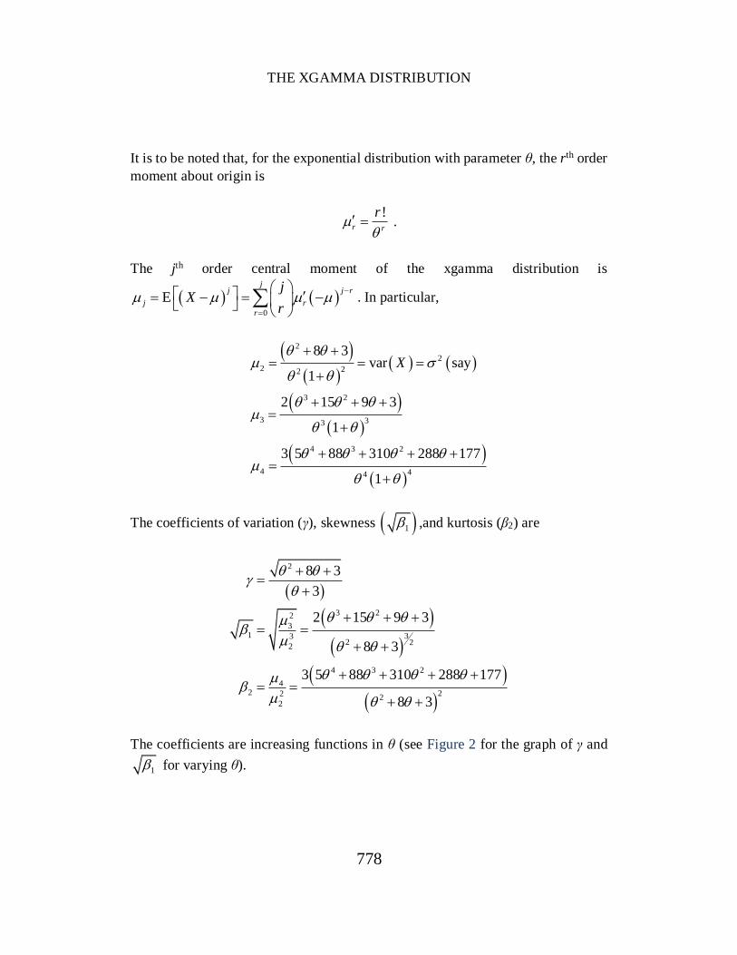
It is to be noted that, for the exponential distribution with parameter θ, the rth order
moment about origin is
!
r r
r
.
The jth order central moment of the xgamma distribution is
0
Ej
j j r
j r
r
jX
r
. In particular,
2
2
2 22
3 2
3 33
3 2
4 44
8 3var say
1
2 15 9 3
1
3 5 88 310 288 177
1
X
The coefficients of variation (γ), skewness 1 ,and kurtosis (β2) are
2
3 22
31 33
2 22
4 3 2
42 22 2
2
8 3
3
2 15 9 3
8 3
3 5 88 310 288 177
8 3
The coefficients are increasing functions in θ (see Figure 2 for the graph of γ and
1 for varying θ).

SEN ET AL
779
Figure 2. Coefficients for variation and skewness
Remark: It should be noted that the values of γ, 1 , and β2 for the
exponential distribution are 1, 2, and 6, respectively. Hence the xgamma
distribution is again more flexible than the exponential distribution.
Survival Properties
The hazard rate function or failure rate function for a continuous distribution with
pdf f(x), cdf F(x), and survival function (sf) S(x) is defined as
0
P | f fh lim
1 F Sx
X x x X x x xx
x x x
.
For the xgamma distribution, the hazard rate function is given by

THE XGAMMA DISTRIBUTION
780
2 2
2 2
12
h
12
x
xx
x
(4)
It is to be noted that
i.
2
h 0 f 01
ii. h(x) is an increasing function in x and θ with θ2/(1 + θ) < h(x) < θ
Remark: For the exponential distribution with parameter θ, h(x) = θ, and so
(4) shows the flexibility of the xgamma distribution over the exponential
distribution. Figure 3 shows the hazard rate function of the xgamma distribution for
selected values of θ.
Figure 3. Hazard rate function of xgamma(θ) for selected values of θ

SEN ET AL
781
Figure 4. Mean residual life function plot of xgamma(θ) for selected values of θ
For a continuous random variable X with pdf f(x) and cdf F(x), the mean
residual life (mrl) function is defined as
1
m E | 1 F1 F
x
x X x X x t dtx
.
For the xgamma distribution, the mrl function (see Figure 4) is given by
2 2
2 2
2 2
11 e
21 e
2
1
12
x
x x
xm x x
xx
x x
xx
(5)
It is to be noted that

THE XGAMMA DISTRIBUTION
782
i.
3m 0
1
ii. m(x) is decreasing in x and θ with
31m
1x
Remark: For the exponential distribution, the mrl function is 1/θ and hence
(6) again shows the flexibility of the xgamma distribution over the exponential
distribution.
Stochastic Ordering
For a positive continuous random variable, stochastic ordering is an important tool
for judging the comparative behavior. Recall some basic definitions:
A random variable X is said to be smaller than a random variable Y in the
i. stochastic order (X ≤st Y) if FX(x) ≥ FY(x) for all x
ii. hazard rate order (X ≤hr Y) if hX(x) ≥ hY(x) for all x
iii. mean residual life order (X ≤mrl Y) if mX(x) ≤ mY(x) for all x
iv. likelihood ratio order (X ≤lr Y) if fX(x)/fY(x) decreases in x
The following implications (see Shaked & Shanthikumar, 1994) are well
justified:
lr hr mrl
hr st
,X Y X Y X Y
X Y X Y
(6)
The following theorem shows that the xgamma distributions are ordered with
respect to the strongest likelihood ratio ordering.
Theorem 1. Let X ~ xgamma(θ1) and Y ~ xgamma(θ2). If θ1 > θ2 then X ≤lr Y
and hence the other ordering in (7).
Proof: Note that
2 1
2 2
1 2 1
2 2
2 1 2
1 2fe , 0
f 1 2
xX
Y
xxx
x x

SEN ET AL
783
2 1
2211 2
2 1 22 2 22 1 2 2
2f 1 40
f 1 2 2
xX
Y
xxd xe
dx x x x
since θ1 > θ2. Hence
f
fX
Y
x
x decreases in x and X ≤lr Y. The remaining
statement follows from (7) directly.
Estimation of the Parameter
Given a random sample X1, X2,…, Xn of size n from the xgamma distribution in (2),
the method of moment (mom) estimator for the parameter θ of xgamma distribution
given in (2) is obtained as follows:
Equate sample mean 1
ni
i
XX
n with first order moment about origin of
(2) which gives the mom estimator of θ as
2
mom
1 1 12ˆ , 0
2
X X XX
X
.
The following theorem shows that the mom estimator of θ in (2) is positively
biased:
Theorem 2. The method of moment estimator of the xgamma distribution is
positively biased, i.e., momˆE 0 .
Proof: Let momˆ g X and
2
1 1 12g
2
t t tt
t
. For t > 0, g''(t) > 0
and hence g(t) is strictly convex. Thus by Jensen’s inequality, we have
g E E gX X . Now since g E g g 3 / 1X ,
we obtain momˆE 0 . Hence the proof.
It should be noted that the sample raw moments are unbiased and consistent
estimators of the corresponding population raw moments. They are also

THE XGAMMA DISTRIBUTION
784
asymptotically normally distributed (CAN estimators) by virtue of the central limit
theorem. Thus the mom estimator, mom , of θ for xgamma distribution is consistent.
Let x = (x1, x2,…, xn) be n observations on a random sample X1, X2,…, Xn of
size n drawn from the xgamma distribution in (2). The maximum likelihood
estimator (mle) of θ for given x is as follows:
The likelihood function is given by
22
1 2
1
L | , , , L | 1 e1 2
i
nx
n i
i
x x x x x
.
The log-likelihood function is given by
2
e
1 1
log L | 2 log log 1 log 12
n n
i i
i i
n n x x
x . (7)
The log-likelihood equation corresponding to (7) becomes
l | log L | 0e
dx
d
x ,
where l(θ | x) is given by
2
21 1
22
11
2
in n
i
i ii
xn n
x
x
To obtain the mle of θ, mle (say), we can maximize (8) directly with respect to θ
or we can solve the non-linear equation l(θ | x) = 0. Note that mle cannot be solved
analytically; numerical iteration techniques, such as the Newton-Raphson
algorithm, are thus adopted to solve the log-likelihood equation for which (8) is
maximized. The initial solution for such an iteration can be taken as:
0
1
n
ii
n
x
.

SEN ET AL
785
Using this initial solution, we have
1
1
1
|
|
i
i i
i
1 x
1 x
for the ith iteration. We choose θ(i) such that θ(i) ≅ θ(i – 1).
Remark. The method of moment and maximum likelihood estimators of the
exponential distribution is 1 X , which is also biased and consistent.
Simulation Study
The inversion method for generating random data from the xgamma distribution
fails because the equation F(x) = u, where u is an observation from the uniform
distribution on (0, 1), cannot be explicitly solved in x. However, we can use the fact
that the xgamma distribution is a special mixture of the exponential(θ) and
gamma(3, θ) distributions.
To generate random data Xi, i = 1, 2,…, n, from the xgamma distribution with
parameter θ, we can use the following algorithm:
1. Generate Ui ~ uniform(0, 1), i = 1, 2,…, n
2. Generate Vi ~ exponential(θ), i = 1, 2,…, n
3. Generate Wi ~ gamma(3, θ), i = 1, 2,…, n
4. If Ui ≤ θ/(1 + θ), then set Xi = Vi. Otherwise, set Xi = Wi
A Monte Carlo simulation study was carried out considering N = 10000 times for
selected values of n and θ. Samples of sizes 20, 40, and 100 were considered and
values of θ were taken as 0.1, 0.5, 1.0, 1.5, 3, and 6 .The following two measures
were computed:
i. Average bias of the simulated estimates ˆi , i = 1, 2,… N:
1
1 ˆN
iiN
ii. Average Mean Square Error (MSE) of the simulated estimates ˆi ,
i = 1, 2,… N: 2
1
1 ˆN
iiN

THE XGAMMA DISTRIBUTION
786
Table 1. Average bias and MSE of the estimator θ
n 20 40 100
theta Bias MSE Bias MSE Bias MSE
0.1 0.00193 0.00020 0.00078 0.00009 0.00034 0.00004
-0.06375 0.00409 -0.06420 0.00414 -0.06438 0.00415
0.5 0.01182 0.00595 0.00539 0.00275 0.00199 0.00106
-0.27887 0.07934 -0.28258 0.08057 -0.28455 0.08125
1.0 0.02655 0.02750 0.01347 0.01290 0.00517 0.00499
-0.48093 0.24223 -0.49040 0.24558 -0.49631 0.24828
1.5 0.04411 0.07234 0.02804 0.03395 0.00871 0.01221
-0.63116 0.43490 -0.64478 0.43260 -0.65975 0.44133
3.0 0.12181 0.36497 0.05765 0.15694 0.02204 0.05985
-0.88938 1.04281 -0.94784 1.00708 -0.98001 1.00190
6.0 0.27864 1.75155 0.14144 0.78423 0.05511 0.28684
-1.06299 2.59379 -1.19641 2.09340 -1.28001 1.88262
The result of the simulation study has been tabulated in Table 1. In Table 1,
for each selected value of θ, the corresponding values relating to the xgamma
distribution have been presented in first row and that relating to exponential
distribution in second row.
Remarks. i) Table 1 shows that the bias is positive in the case of the xgamma
distribution (as shown in the Theorem 2). Table 1 also shows that bias and MSE
decreases as n increases and increases when θ increases. ii) In terms of bias and
MSE of the estimates of θ, the xgamma distribution shows more flexibility as
compared to the exponential distribution.
Application
In this section, a real data set is used to show that the xgamma distribution can be
a better model than one based on the exponential distribution. The data on relief
times (in hours) of 20 patients receiving an analgesic (cf. Gross & Clark, 1975) is
used. Both the xgamma and exponential distributions are fitted to this data set. The
method of maximum likelihood is used. Maximum likelihood estimates for both
the cases are calculated for the data. The required numerical evaluations are carried
out using R 3.1.1 software. Table 2 provides the maximum likelihood estimates
with corresponding standard errors of the model parameters. The model selection
is carried out using the log-likelihood value, AIC (Akaike information criterion),
the AICc (consistent Akaike information criteria) and the BIC (Bayesian
information criterion):

SEN ET AL
787
e e e
2 1AIC 2log 2 , AICc AIC , BIC log 2log
1
k kL k k n L
n k
where logeL denotes the log-likelihood function evaluated at the maximum
likelihood estimates, k is the number of parameters, and n is the sample size.
From Table 2, it is clear that the values of the AIC, AICc and BIC are smaller
for the xgamma distribution compared with those values of the exponential model,
so the new distribution seems to be a very competitive model to these data. It
follows that the xgamma distribution provides the better fit to the data. Table 2. Maximum likelihood estimates and model selection statistics
Distributions
Maximum Likelihood Estimates
Standard Error
Log-likelihood AIC AICc BIC
Exponential θmle
= 0.52632 0.11769 -32.83708 67.67416 67.89638 68.66989
xgamma θmle
= 1.10747 0.16943 -31.50824 65.01649 65.23871 66.01221
Conclusion
The xgamma distribution, a special finite mixture of exponential and gamma
distributions, was derived. Various mathematical and structural properties of the
distribution were studied including the shape, moments, measures of skewness, and
kurtosis. Important survival properties like the hazard rate and mean residual life
functions were derived and discussed. Stochastic ordering and a simulation
algorithm were also proposed. Added flexibility over the exponential distribution
was observed with regard to certain important properties of the xgamma
distribution. The maximum likelihood method and method of moments were
proposed for the parameter estimation. In order to demonstrate the applicability of
the xgamma distribution, a simulation study was shown. Moreover, the distribution
was fitted to a real data set and compared with the exponential distribution. Results
show that the xgamma distribution provides an adequate fit for the data set. The
maximum likelihood functions may be further studied under different types of
censoring mechanism for future applications of the xgamma model. Bayesian
estimation of the parameter of xgamma distribution may further be considered with
suitable prior and risk function.

THE XGAMMA DISTRIBUTION
788
References
Barlow, R. E., & Proschan, F. (1981). Statistical theory of reliability and life
testing: Probability models. Silver Spring, MD: To Begin With.
Everitt, B. S. (1996). An introduction to finite mixture distributions.
Statistical Methods in Medical Research, 5(2), 107-127. doi:
10.1177/096228029600500202
Everitt, B. S., & Howell, B. (Eds.). (2005). Encyclopedia of statistics in
behavioral science. Hoboken, NJ: John Wiley & Sons.
Gross, A. J., & Clark, V. A. (1975). Survival distributions: Reliability
applications in the biomedical sciences. New York, NY: John Wiley & Sons.
Johnson, N. L., Kotz, S., & Balakrishnan, N. (1994). Continuous univariate
distributions (Vol. 1) (2nd ed.). New York, NY: Wiley.
Johnson, N. L., Kotz, S., & Balakrishnan, N. (1995). Continuous univariate
distributions (2nd ed.) (Vol. 2). New York, NY: Wiley.
Lawless, J. F. (2003). Statistical models and methods for lifetime data (2nd
ed.). New York, NY: John Wiley & Sons.
McLachlan, G., & Peel, G. (2000). Finite mixture models. New York, NY:
John Wiley & Sons.
Shaked, M., & Shanthikumar, J. G. (1994). Stochastic orders and their
applications. New York, NY: Academic Press.