The WiggleZ Dark Energy Survey: improved distance ...

MNRAS 441, 3524–3542 (2014) doi:10.1093/mnras/stu778

The WiggleZ Dark Energy Survey: improved distance measurements toz = 1 with reconstruction of the baryonic acoustic feature

Eyal A. Kazin,1,2‹ Jun Koda,1,2 Chris Blake,1 Nikhil Padmanabhan,3 Sarah Brough,4

Matthew Colless,4 Carlos Contreras,1,5 Warrick Couch,1,4 Scott Croom,6

Darren J. Croton,1 Tamara M. Davis,7 Michael J. Drinkwater,7 Karl Forster,8

David Gilbank,9 Mike Gladders,10 Karl Glazebrook,1 Ben Jelliffe,6 Russell J. Jurek,11

I-hui Li,12 Barry Madore,13 D. Christopher Martin,8 Kevin Pimbblet,14,15

Gregory B. Poole,1,16 Michael Pracy,1,6 Rob Sharp,16,17 Emily Wisnioski,1,18

David Woods,19 Ted K. Wyder8 and H. K. C. Yee12

Affiliations are listed at the end of the paper

Accepted 2014 April 17. Received 2014 March 14; in original form 2013 December 31

ABSTRACTWe present significant improvements in cosmic distance measurements from the WiggleZDark Energy Survey, achieved by applying the reconstruction of the baryonic acoustic featuretechnique. We show using both data and simulations that the reconstruction technique canoften be effective despite patchiness of the survey, significant edge effects and shot-noise.We investigate three redshift bins in the redshift range 0.2 < z < 1, and in all three findimprovement after reconstruction in the detection of the baryonic acoustic feature and itsusage as a standard ruler. We measure model-independent distance measures DV(rfid

s /rs)of 1716 ± 83, 2221 ± 101, 2516 ± 86 Mpc (68 per cent CL) at effective redshiftsz = 0.44, 0.6, 0.73, respectively, where DV is the volume-averaged distance, and rs is thesound horizon at the end of the baryon drag epoch. These significantly improved 4.8, 4.5 and3.4 per cent accuracy measurements are equivalent to those expected from surveys with upto 2.5 times the volume of WiggleZ without reconstruction applied. These measurements arefully consistent with cosmologies allowed by the analyses of the Planck Collaboration andthe Sloan Digital Sky Survey. We provide the DV(rfid

s /rs) posterior probability distributionsand their covariances. When combining these measurements with temperature fluctuationsmeasurements of Planck, the polarization of Wilkinson Microwave Anisotropy Probe 9, andthe 6dF Galaxy Survey baryonic acoustic feature, we do not detect deviations from a flat �

cold dark matter (�CDM) model. Assuming this model, we constrain the current expansionrate to H0 = 67.15 ± 0.98 km s−1Mpc−1. Allowing the equation of state of dark energy tovary, we obtain wDE = −1.080 ± 0.135. When assuming a curved �CDM model we obtain acurvature value of �K = −0.0043 ± 0.0047.

Key words: cosmological parameters – distance scale – large-scale structure of the universe.

1 IN T RO D U C T I O N

The baryonic acoustic feature is regarded as a reliable tool formeasuring distances, which can be used to probe cosmic expansionrates and hence assist in understanding the mysterious nature ofthe recent cosmic acceleration (Riess et al. 1998; Perlmutter et al.

� E-mail: [email protected]

1999; Blake & Glazebrook 2003; Seo & Eisenstein 2003). Earlyplasma-photon acoustic waves that came to a near-stop at a redshiftz ∼ 1100 left these baryonic signatures imprinted at a comovingradius of ∼150 Mpc in both the cosmic microwave background(CMB) temperature fluctuations and in the distribution of matter, asan enhancement in the clustering amplitude of overdensities at this‘standard ruler’ distance (Peebles & Yu 1970).

However, the signature in the distribution of matter, and hence ingalaxies, experienced a damping due to long-range coherent bulk

C© 2014 The AuthorsPublished by Oxford University Press on behalf of the Royal Astronomical Society

at California Institute of T

echnology on August 7, 2014

http://mnras.oxfordjournals.org/

Dow

nloaded from

mailto:[email protected]


Reconstructed WiggleZ 3525

motions generated by tidal gravitational forces. In the linear densityfield, galaxies coherently move by ∼5 Mpc from their originalpositions, which causes smoothing of the otherwise sharp feature atthe scale of 150 Mpc in the clustering correlation function. Althoughthis damping is well understood and modelled (Meiksin, White &Peacock 1999; Seo & Eisenstein 2007; Angulo et al. 2008; Crocce &Scoccimarro 2008; Sanchez, Baugh & Angulo 2008; Seo et al. 2008;Smith, Scoccimarro & Sheth 2008; Kim et al. 2009), it decreasesthe accuracy with which the feature may be used as a standard ruler.

To correct for the effects of large-scale motions, Eisenstein et al.(2007) suggested the method of reconstruction of the baryonicacoustic feature. By using the density field to infer the displace-ments caused by these bulk flows in linear theory, one can retractthe galaxies to their near-original positions, and hence sharpen thebaryonic acoustic signature. They concluded that this method im-proves the usage of the baryonic acoustic feature as a standard ruler.The technique has since been further developed, showing that thisprocedure minimizes the systematic errors in the bias of geomet-ric information obtained from matter and galaxies (Noh, White &Padmanabhan 2009; Padmanabhan, White & Cohn 2009; Seo et al.2010; Mehta et al. 2011). Mehta et al. (2011) concluded that dis-tance measurements made when using galaxies with a low galaxy tomatter density bias of b = δgal/δm ∼ 1, such as those analysed here,have a low systematic error of ∼0.2–0.25 per cent which is reducedto 0.1–0.15 per cent when applying reconstruction (see their fig. 5).

The first successful application of the technique to galaxy datawas reported by Padmanabhan et al. (2012), who improved the dis-tance constraint to z = 0.35 by sharpening the baryonic acousticfeature of the luminous red galaxy sample (Eisenstein et al. 2001)of the SDSS-II (York et al. 2000). Testing realistic mock catalogues,they showed that the technique yields unbiased improved results. Afurther application of the technique was performed by the SDSS-IIIBaryon Oscillation Spectroscopic Survey (BOSS) using a massivegalaxy sample at z = 0.57 (Anderson et al. 2012, 2014b). Theinability of the technique to improve constraints in this particularcase may be attributed to sample variance in the sense that thepre-reconstruction measurement was on the fortunate side of ex-pectations (Kazin et al. 2013). Recently the BOSS Collaborationhave shown this to be the mostly likely explanation, by showingimprovement of distance measures when probing galaxy samplestwo and three times as large (Anderson et al. 2014a, see their fig. 4.)

In this study, we apply the reconstruction technique to galaxiesmapped by the WiggleZ Dark Energy Survey (Drinkwater et al.2010). The 0.2 < z < 1 range of WiggleZ enables the survey toprobe dark energy at a unique effective redshift of z = 0.73, whichis close to the beginning of the acceleration phase, according to thedark energy cold dark matter (CDM) paradigm. We have previouslyreported measurements using the baryonic acoustic feature in thisredshift range with accuracies of ∼4.5–7.5 per cent (Blake et al.2011). In this analysis, we show that reconstruction improves thedetectability of the baryonic acoustic feature and yields substan-tially tighter distance constraints.

When applying reconstruction to WiggleZ we are confrontedby various challenges compared to other galaxy surveys. TheWiggleZ volumes are patchy with substantial edge effects, becauseeach survey region is only ∼500 h−1Mpc in dimension with ad-ditional incompleteness due to the input catalogues. In addition,clustering measurements using the highest redshifts of the volumealso contain fairly high shot-noise corresponding to nP ∼ 1, wheren is the number density and P is the characteristic power spec-trum amplitude at wavenumber k ∼ 0.15 h Mpc−1. Hence, we arerequired to test if reconstruction of the density fields of such vol-

umes could potentially cause possible biases when displacing thegalaxies.

To test for this, we apply the algorithm to a myriad of realisticsimulated realizations. Constructing mock catalogues from N-bodysimulations for WiggleZ is a challenging problem because the galax-ies trace dark matter haloes with masses ∼1012 h−1 M�, an orderof magnitude lower than those populated by luminous red galaxies.For this reason, in past analyses of WiggleZ (e.g. Blake et al. 2011)we used log-normal realizations to support the data analysis (e.g. todetermine the covariance of the measurement). These, however, donot contain realistic displacement information. Hence, to supportthis study we generated 600 mock realizations based on a moreaccurate Lagrangian comoving scheme, as described in Section 2.2.

Another difference between the past and current WiggleZ anal-yses is the manner in which we model the correlation function ξ .In past analyses, we modelled the full shape, resulting in model-dependent measurements. The reason for this is that when assuminga theoretical model for ξ its full shape may be used as a standardruler (e.g. see Eisenstein et al. 2005; Sanchez et al. 2012, 2013). Asreconstruction involves smoothing of the density field, it is difficultto model the overall broad-band shape of the post-reconstructionpower spectrum. For this reason, in this analysis we are only in-terested in the baryonic acoustic peak position, and hence focuson the geometric information. This means that we are required tomarginalize over the shape information, which makes the distancemeasurements reported here model independent.

This study is presented as follows. In Section 2, we present thedata, simulated data, the reconstruction technique and the construc-tion of the two-point correlation functions. In Section 3, we describethe method used to calculate the geometric constraints, includingthe construction of the fitting model. In Section 4, we present dis-tance measurements from the data and compare with those obtainedwith the simulations. This section is concluded by cosmological im-plications. We summarize in Section 5.

Unless otherwise stated, we assume a flat �CDM fiducial cos-mology as defined in Komatsu et al. (2009): a dark matter densityof �m = 0.27, a baryon density of �b = 0.0448, a spectral indexof ns = 0.963, an rms of density fluctuations averaged in spheresof radii at 8 h−1Mpc of σ 8 = 0.8 and h = 0.71, where the localexpansion rate is defined as H0 = 100h kms−1 Mpc−1.

2 DATA

2.1 Galaxy sample

The WiggleZ Dark Energy Survey (Drinkwater et al. 2010) is alarge-scale galaxy redshift survey of bright emission-line galaxiesover the redshift range z < 1, which was carried out at the Anglo-Australian Telescope between 2006 August and 2011 January. Intotal, of the order of 200 000 redshifts of UV-selected galaxies wereobtained, covering of order 1000 deg2 of equatorial sky. In thisstudy, we analyse the same final WiggleZ galaxy sample as utilizedby Blake et al. (2011) for the measurements of baryonic acousticoscillations (BAOs) in the galaxy clustering pattern. After cuts tomaximize the contiguity of the observations, the sample contains158 741 galaxies divided into six survey regions – the 9-h, 11-h,15-h, 22-h, 1-h and 3-h regions. The survey selection function withineach region was determined using the methods described by Blakeet al. (2012).

For purposes of this study, following the analysis of Blake et al.(2011), we divided the galaxies into three redshift bins of width�z = 0.4, defined here as: �zNear (0.2 < z < 0.6), �zMid

MNRAS 441, 3524–3542 (2014)




Dow

nloaded from


3526 E. A. Kazin et al.

(0.4 < z < 0.8) and �zFar (0.6 < z < 1.0). Note that thesecond bin fully overlaps with the other two, which are independentfrom each other.

Blake et al. (2011) calculated the effective redshift zeff of ξ ineach slice as the weighted mean redshift of the galaxy pairs in theseparation bin 100 < s < 110 h−1Mpc, where the z of a pair is theaverage (z1 + z2)/2. For �zNear, �zMid and �zFar, this results inzeff = 0.44, 0.6 and 0.73, respectively.

2.2 The WiZ-COLA simulation

Simulated galaxy catalogues are a key tool for interpretation oflarge-scale structure measurements which are used to determinecovariances, and test methodologies for potential biases. In thissection, we briefly describe the construction of the mock cataloguesused in this analysis. For full details, the reader is referred to Kodaet al. (in preparation).

Constructing hundreds of mock catalogues from N-body simu-lations for WiggleZ is a challenging problem because the galaxiestrace dark matter haloes with masses ∼1012 h−1 M�, an order ofmagnitude lower than those populated by luminous red galaxies.For this reason, we employed cheaper methods of production ofmocks that yield a good approximation to N-body simulations.

In our first attempt to build mock catalogues, we tried imple-menting the second-order Lagrangian Perturbation Theory method(Bernardeau et al. 2002), as described in Manera et al. (2013). How-ever, we found that because of poor resolution, this method failedto identify correctly low-mass haloes such as those in which thelow-bias WiggleZ galaxies reside.

For this reason, we developed a parallel version of the COmovingLagrangian Acceleration simulation (COLA; Tassev, Zaldarriaga& Eisenstein 2013) which we used to generate 3600 realizationsof 10-time step simulations – 600 realizations for each of the sixobservational regions in the WiggleZ survey.

Each of the WiggleZ COLA ( WiZ-COLA) simulations consistsof 12963 N-body particles in a box of 600 h−1 Mpc on a side, whichgives a particle mass of 7.5 × 109 h−1 M�. We use 3 × 1296 gridsper dimension to calculate the gravitational force with enough spa-tial resolution (Tassev et al. 2013). This simulation configurationhas sufficient volume to contain one region of the WiggleZ surveyfor each redshift range z = 0.2–0.6, 0.4–0.8 or 0.6–1.0, and simul-taneously resolves dark matter haloes down to 1012 h−1 M�, whichhost emission-line galaxies observed in the WiggleZ survey. Eachsimulation takes 15 min with 216 computation cores, including halofinding.

As fully described in Koda et al. (in preparation), we populatethe haloes using a Gaussian halo occupation distribution, such thatthe resulting projected correlation functions wp(rp) match thoseof the observations.

We then apply the WiggleZ selection function to the mock galax-ies to make simulated catalogues with correct survey geometry.When we apply the mask, we rotate the simulation box to fit thesurvey volume into the box with minimum overlap, using the remap-ping algorithm by Carlson & White (2010) to find the best rotation.We output three snapshots at z = 0.44, 0.6 and 0.73, for the threeredshift bins, �zNear, �zMid and �zFar, respectively. In eachredshift bin, we use the appropriate independent 600 mocks to gen-erate covariance matrices, as described in Sections 2.4 and 3.2, andanalyse each redshift bin separately to measure DV/rs (as definedbelow).

Our simulation box is large enough for one redshift bin, but notfor the full range 0.2 < z < 1. This is not a problem when we

treat different redshifts separately (Sections 4.1 and 4.2), but doesnot give the correct correlation between �zMid and the other tworedshift bins. For this reason, we also create 300 additional mockcatalogues for each of the six regions to evaluate the correlationcoefficient between the DV/rs measurements in the overlappingredshift regions (as presented in Section 4.5). We combine, or stitch,two mock catalogues from different realizations of z = 0.2–0.6 andz = 0.6–1.0, by joining them together at their sharp edges of z = 0.6and cut out the redshift region z = 0.4–0.8 appropriately from each.This mock does not have accurate clustering across the boundaryat z = 0.6, but contains the same mock galaxies that exist in theother two redshift regions 0.2–0.6 and 0.6–1.0, which is necessaryto compute the correlation between the overlapping redshift data.Because for each of the 600 realizations we use different snap-shots to create the three original �z volumes, by stitching �zNear

and �zFar from different realizations we end up with 300 stitchedversions.

2.3 Reconstruction of the density field

In order to reduce effects of large-scale coherent motions on thebaryonic acoustic feature, the reconstruction of the density fieldmethod is applied by shifting the galaxies to their near-originalpositions in the linear density field. Here, we describe the calculationof the displacement vectors from the density fields, including thesurvey selection effects.

We determine the displacement field � within the Zel’dovichapproximation (Zel’dovich 1970) following the method describedby Padmanabhan et al. (2012). Given that large-scale structure out-side the survey regions contributes gravitationally to displacementswithin, it is necessary to enclose the observed volume within alarger ‘embedded’ volume, into which we must extrapolate the den-sity field in a statistically consistent manner. The extrapolation isover any unobserved regions inside the survey cone, and into a‘padding’ volume which extends 200 h−1 Mpc beyond each edge ofa cuboid enclosing the survey region. For each of the 18 volumesanalysed (6 angular regions and 3 redshift slices), we apply thereconstruction technique described here independently, because wedo not expect volumes to affect each other due to the large distancesbetween them.

We summarize the steps of the method as follows, distinguish-ing between quantities evaluated over the observed and embeddedvolumes.

(i) We evaluate the smoothed, observed galaxy overdensity field,δ(x), in each survey region. We carry out this calculation by bin-ning the galaxy distribution and normalized selection function ina 3D comoving coordinate grid with a cell size of 5 h−1Mpc onthe side, denoting these gridded distributions as Dc and Rc (wherec is the cell number), and then determining δ by smoothing thesedistributions with a Gaussian kernel G(x) = e−(x·x)/2λ2

such thatδc = smooth(Dc)/smooth(Rc) − 1 and 〈δc〉 = 0. We choose an rmssmoothing scaling λ = 15 h−1Mpc for our analysis, noting that ourresults are not sensitive to this choice. From here on we drop the ‘c’notation from δ, for convenience.

(ii) We generate a realization of an ‘unconstrained’ Gaussianrandom field across the embedded volume, δU , using an assumedgalaxy power spectrum P(k) consistent with fits to the data in theobserved region. We smooth the unconstrained overdensity field inthe same manner as the observed overdensity field.

MNRAS 441, 3524–3542 (2014)




Dow

nloaded from



(iii) We use the Hoffman–Ribak algorithm (Hoffman & Ribak1991; equation 3 in Padmanabhan et al. 2012), as our best estimateof the overdensity field in the embedded volume:

δ = δU + C C−1(δ − PδU ), (1)

where P is a matrix of zeros and ones which projects a vector fromthe embedded volume to the observed volume, and C and C arethe covariance matrices of pixels in the observed and embeddedvolumes, respectively, which are just the correlation functions ξ :

Cij = 〈δ(xi) δ(xj )〉 = ξ (|xi − xj |). (2)

Following Padmanabhan et al. (2012), we solve equation (1) in anumber of steps. (i) We evaluate u = δ − PδU by simple projectionof δU from the embedded to the observed volumes. (ii) We solvev = C−1u using a preconditioned conjugate gradient algorithm todetermine the solution of Cv = u, using a modified version of theNumerical Recipes subroutine linbcg. For each iteration, the ex-pression Cv is evaluated by fast Fourier transforms, using the factthat multiplication by C is equivalent to convolution by ξ (r). There-fore, FT(Cv) is equal to the product of P(k) and FT(v), where wenote that the power spectra contain the galaxy shot-noise contribu-tion 1/n in terms of mean galaxy density n. (iii) We project v intothe embedded space, v = P−1v, and calculate w = Cv as above.(iv) The final overdensity field in the embedded volume is given byδ = δU + w.

(iv) Finally, we estimate the displacement field � in theZel’dovich approximation as

∇ · � + (f /b) ∇ · (s s) = −δ/b, (3)

where f is the growth rate of structure at the survey redshift, bis the galaxy bias factor and s = � · s is the displacement inthe line-of-sight direction. We assume values f = 0.70 (z = 0.44),0.76 (z = 0.6), 0.79 (z = 0.73) and b = 1, 1.1, 1.2 (for �zNear,�zMid and �zFar, respectively), noting that our results are notsensitive to these choices. The flat-sky approximation is valid forthe WiggleZ survey regions, and we can therefore take the line-of-sight direction as parallel to a single Cartesian axis, which we takeas the x-direction, such that s = � · x. We then solve equation (3)by substituting � = ∇φ and taking the Fourier transform of theequation to obtain

[(1 + f /b)k2

x + k2y + k2

z

]FT[φ](kx, ky, kz) = FT[δ](kx, ky, kz)

b,

(4)

where FT is the Fourier transform.The inverse Fourier transform then yields the displacement field�(x, y, z) = ∇φ.

(v) We then shift each galaxy and random point by −�. Tosubtract the Kaiser effect in redshift space, the galaxies are alsoshifted an additional −fx in the x dimension. This additional shiftis not applied to the random points.

At the end of this procedure, for each of the 18 volumes, we obtaina shifted data catalogue and a shifted random point catalogue.

2.4 Correlation functions

To estimate the correlation function, we compare pair counts ofthe data to those of a sample of random points. The random pointsare distributed in a Poisson-like manner, such that they trace themask of the survey, as described in Blake et al. (2012). To reduce

shot-noise effects of the mask, we use a ratio of 100 random pointsper data point.

Before calculating pairs, we first convert the data and randomsfrom the R.A, Dec., z coordinate system to a comoving Euclidiansystem assuming a flat �CDM fiducial cosmology as defined inKomatsu et al. (2009): �m = 0.27. When calculating the pairs,each galaxy and random point is assigned a weight according to theFeldman, Kaiser & Peacock (1994) minimum variance weighting,which takes into account the number density at a given redshiftn(z):

w(z) = 1

1 + P · n(z), (5)

where we assume P = 5000 h−3 Mpc3 as the characteristic powerspectrum amplitude at the physical scales of interest.

We calculate the Landy & Szalay (1993) correlation functionestimator ξ for each of the 18 volumes. This is done first bycalculating:

ξ (μ, s) = DD − 2DR + RRnum

RRdenom, (6)

where the line-of-sight direction μ = 1 is defined as the directionwhich bisects the separation vector s between each pair, and s ≡ |s|.The normalized galaxy–galaxy pair count is DD(μ, s) and similarlyfor the normalized galaxy–random DR and normalized random–random RR counts.

The reconstruction procedure described in Section 2.3 results invarious data and random sets which we use as follows. For thepre-reconstruction case, we use the original data and random pointcounts where both RR terms in equation (6) are the same. In thereconstruction case, we use the shifted data for DD and DR, andshifted randoms for DR and RRnum. Finally, for the RRdenom term,we use the original non-shifted randoms. In this study, we examineresults using two different separation bin widths �s, of 3.3 h−1Mpcand 6.7 h−1Mpc.

To account for the volume limitation of each region, the integralconstraint correction is calculated as

I .C =∑

siξ theory(si)RRnum(si)∑

siRRnum(si)

(7)

and added to ξ (μ, s). For this purpose, the RR terms used arecalculated in each region to a large separation s at which RR is zero.In the largest region, this is just over 1 h−1Gpc. The theoreticalmodel used, ξ theory, is a combination of the template used in theanalysis for s > 50 h−1Mpc (see Section 3.1), and a linear modelfor lower separation bins si. For the reconstruction case, we use theshifted random point count RR, and do not include the Kaiser boostterm in ξ theory. We verify that the resulting values of I.C are notsensitive to details of this procedure.

We then obtain the angle-averaged correlation function ξ 0 andquadrupole ξ 2 of each of the 18 volumes by integrating eachξ (μ, s) using the appropriate Legendre polynomials. We followthis procedure for both the data and the 600 mock catalogues, per-forming measurements before and after reconstruction.

To calculate the three redshift slice correlation functions ξ�z,we combine the correlation functions of six angular regions � inthe following manner. To account for the correlations between themultipoles (Taruya, Saito & Nishimichi 2011; Kazin, Sanchez &Blanton 2012), we define the vector ξ�

[0,2] that contains ξ�0 and ξ�

2

and therefore has a length equal to double the number of bins.We emphasize that we use the ξ�

2 information to construct the ξ�z0

because the multipoles are not independent, as shown below.

MNRAS 441, 3524–3542 (2014)




Dow

nloaded from



Figure 1. The top and centre panels show the normalized covariance matrix Cij[0,2]/

√Cii

[0,2]Cjj[0,2] before and after reconstruction, respectively, for each of the

�z volumes, as indicated. The bottom panels show comparisons of S/N ratios of the monopole |ξ0|/σξ0 , before (dashed red) and after reconstruction (solidblue), where we define the uncertainties σξ0 = √

Cii of the ‘0’ component.

The resulting covariance matrix C[0,2] is defined as

C�[0,2]ij

= 1

Nmocks − 1

Nmocks∑m=1(

ξ�[0,2]i

− ξ� m[0,2] i

) (ξ�

[0,2]j− ξ� m

[0,2] j

), (8)

where the over-line denotes the mean value of Nmocks = 600.Following White et al. (2011), we then combine these to obtain

ξ�z[0,2] = C�z

[0,2]

∑�

(C�

[0,2]

)−1ξ�

[0,2], (9)

where(C�z

[0,2]

)−1 =∑

�

(C�

[0,2]

)−1. (10)

Fig. 1 displays the resulting C�z[0,2] for all three redshift volumes. The

top and centre row of panels show the normalized values pre- andpost-reconstruction, respectively. The bottom row of panels displaysthe signal-to-noise (S/N) of the monopole defined as |ξ0|/σξ0 , wherethe uncertainty σξ0 is the square root of the diagonal elements of themonopole component of C[0,2].

We notice that the off-diagonal normalized terms in the ξ 0

and ξ 2 quadrants are suppressed in the post-reconstruction casecompared to pre-reconstruction. This can be explained by therestoration of the linear density field and removal of the galaxydisplacements.

The bottom panels of Fig. 1 show clear improvement in theS/N of ξ 0 at the scale of the baryonic acoustic feature in all �z.The improvement with reconstruction is 40 per cent for �zNear,25 per cent for �zMid and 15−25 per cent for �zFar. This is the casefor both separation widths of �s = 3.3 h−1Mpc and 6.7 h−1Mpc. TheS/N is lower at other scales (s < 90 h−1Mpc and s > 130 h−1Mpc)because of the suppression of the redshift-space clustering power.

We defer investigation of the cosmological content of ξ 2 to futurestudies, and from hereon refer to ξ as the angle-averaged measure-ment.

In Fig. 2, we display the resulting angle-averaged correlationfunctions ξ from equation (9) for the data pre- (red squares) andpost-reconstruction (blue circles). The corresponding mean signalof the mock simulations ξ are displayed in Fig. 3.

In each of the three �z bins, we see a sharpening of the baryonicacoustic peak both in the data and in the simulations. In Section 4.1,we quantify this sharpening, and in Section 4.2, we present the

MNRAS 441, 3524–3542 (2014)




Dow

nloaded from



Figure 2. The WiggleZ two-point correlation functions shown before (red squares) and after applying reconstruction (blue circles) for three redshifts binsand the full z range, as indicated. These are plotted as ξs2 to emphasize the region of the baryonic acoustic feature. The uncertainty bars are the square rootof the diagonal elements of the covariance matrix. The solid lines are the best-fitting models to the range of analysis 50 < s < 200 h−1Mpc. We see a clearsharpening of the baryonic acoustic feature after reconstruction in all cases.

improved distance measurements and compare these with expecta-tions according to the mocks.

Comparing results pre- and post-reconstruction of the data andmocks, we also see a clear reduction post-reconstruction in theamplitude of ξ at scales outside the acoustic ring, s < 100 h−1Mpcand s > 140 h−1Mpc. This can be explained by the subtraction ofthe linear redshift distortions, when applying reconstruction.

The negative measurements of ξ at large scales for �zNear, andthe positive measurements for �zFar, are consistent with the ex-pectations of sample variance. This is best understood realizing thefact that the data points are correlated.

The various ξ and their covariance matrices can be found on theWorld Wide Web.1

3 M E T H O D O L O G Y

3.1 Modeling ξ

In our previous analysis of this data in Blake et al. (2011), we treatedthe full shape of ξ as a standard ruler, and modelled the whole cor-

1 http://www.smp.uq.edu.au/wigglez-data/bao-random-catalogues

relation function. In our current analysis, we focus solely on thegeometrical information contained in the baryonic acoustic featureDV/rs (defined below) and marginalize over the information en-coded in the full shape of ξ , e.g. �m h2 and the spectral index ns. Thisis because the reconstruction procedure as described in Section 2.3,while sharpening the baryonic peak and hence improving distanceconstraints, involves a smoothing process which affects the corre-lation function slope in a manner which is difficult to model.

To measure DV/rs for each �z bin, we compare the data ξ�z(si)(described in Section 2.4) to a model ξm(si) defined as:

ξm(sf ) = a0 · ξT(sf/α) + A(sf ), (11)

where ξT is a template correlation function and A(s) is a polynomial,both defined below, and sf is the distance scale in the coordinatesystem of the fiducial cosmology.

As we are interested in the geometrical information encoded inthe baryonic acoustic feature position, not in the full shape of ξ ,we follow the procedure outlined by Xu et al. (2012) in which wemarginalize over the amplitude and shape parameters ai (i = 0, 1,2, 3) as defined by

A(s) = a1 + a2

s+ a3

s2. (12)

MNRAS 441, 3524–3542 (2014)




Dow

nloaded from

http://www.smp.uq.edu.au/wigglez-data/bao-random-catalogues



Figure 3. The mean of the simulated two-point correlation functions shown before (red squares) and after applying reconstruction (blue circles) for threeredshifts bins and the full z range, as indicated. These are plotted as ξs2 to emphasize the region of the baryonic acoustic feature. The uncertainty bars are thesquare root of the diagonal elements of the covariance matrix (for one WiZ-COLA realization, not the mean). The solid lines are the templates ξT used in theanalysis (not the best-fitting model), where we focus on the range of analysis 50 < s < 200 h−1Mpc. For the s < 50 h−1Mpc region, we plot a linear model.We see a clear sharpening of the baryonic acoustic feature after reconstruction in all cases.

All effects on the amplitude, e.g. σ 8, linear bias and linear redshiftdistortions, are contained in a0 which we marginalize over.

The α parameter in equation (11) takes into account the distortionbetween distances measured in the fiducial cosmological modelused to construct the ξ measurement, and the trial cosmologicalmodel we are testing. When applied to the baryonic acoustic feature,Eisenstein et al. (2005) argued that this distortion may be related tothe cosmic distance scale as

α = (DV/rs)

(DV/rs)fid, (13)

where the volume-averaged distance is defined as

DV(z) =(

cz(1 + z)2D2A

H

)1/3

, (14)

where DA(z) is the physical angular diameter distance, H(z) is theexpansion rate and c is the speed of light (as defined in Hogg 1999).The calculation of the sound horizon rs is discussed in Section 4.5.Equation (13) stems from the fact that α is the Jacobian of thevolume element d3s, when transforming between the true coordinatesystem to the fiducial one sf. Anderson et al. (2014b) showed that

this is a fairly good approximation, even when there is anisotropicwarping.

The template ξT we use is based on renormalized perturbationtheory (RPT), as introduced by Crocce & Scoccimarro (2008)

ξT(s) = ξL ⊗ e−(k∗s)2 + AMCξ (1) dξL

ds, (15)

where the ⊗ term denotes convolution, L means linear, and

ξ (1)(s) = s · ∇−1ξL =∫ ∞

0

k

2π2PL(k)j1(ks)dk, (16)

where j1(y) is the spherical Bessel function of order 1.This model has been investigated and applied by Sanchez et al.

(2008, 2009, 2013), who show that it gives an unbiased measure-ment of α, DA, H and the equation of state of dark energy wDE.

To calculate the linear PL and ξL we use the CAMB package2

(Lewis, Challinor & Lasenby 2000) using the fiducial cosmologymentioned in Section 1. The input redshifts chosen for each redshiftbin are the effective values given above.

2 http://camb.info

MNRAS 441, 3524–3542 (2014)




Dow

nloaded from

http://camb.info



Table 1. k∗ values for the RPT ξ templates.

Volume k∗ pre-recon k∗ post-recon

�zNear: 0.2 < z < 0.6 0.17 0.55�zMid: 0.4 < z < 0.8 0.19 0.55�zFar: 0.6 < z < 1 0.20 0.55

k∗ in units of h Mpc−1.

The first term in equation (15) damps the baryonic acousticfeature through the k∗ parameter. The second term takes into accountk-mode coupling (MC) via the AMC parameter.

In our analysis, we fix k∗ and AMC to values corresponding tothe best fits to the signal of the mock-mean correlation function(ξ hereon). These fits are performed using the covariance matrix ofthe mock mean, and marginalizing over the amplitude. The valueof AMC is set to 0.15, and the k∗ values are summarized in Table 1.

In the pre-reconstruction case, we notice that k∗ increases withredshift. This is expected because at higher redshift galaxies haveless time to accumulate a displacement from their bulk flows andhence the damping scale is smaller.

The post-reconstruction fits tend to prefer a much higher k∗(0.55 h Mpc−1) due to the sharpening of the peak. We test thedata and the mock ξ and verify that the parameter of interest in theanalysis, α, is not correlated with k∗ or AMC. This verifies that ourdistance constraints do not depend on our choice of k∗ or AMC.

The resulting templates ξT are displayed as the solid lines inFig. 3, where the upper red is the pre-reconstruction template and thebottom blue is post-reconstruction. The corresponding data pointsare the mock ξ . Although the focus of the analysis is the separationrange s = 50−200 h−1Mpc, we also extrapolate in grey to the regions < 50 h−1Mpc, using a linear model ξL matched in amplitude at50 h−1Mpc (where RPT is no longer valid; Sanchez et al. 2008). Inan analysis using a similar method Kazin et al. (2013) demonstratedthat the geometric information was insensitive to the fitting range aslong as the lower bound is less than 65 h−1Mpc (see their fig. 13).

In Fig. 3, the pre-reconstruction templates show excellent agree-ment with the respective ξ . The post-reconstruction template con-tains a slight downward consistent shift in ξs2 compared to the ξ ,as the fit tends to be dominated by the accurate measurements atlower separations. This offset is easily accommodated by the A(s)terms, and we verify below that any resulting bias in the best-fittingvalues of α is negligible.

3.2 Statistical methods

Throughout this analysis, we define the log-likelihoodχ2 ≡ −2log L, calculated by

χ2(�) =Nbins∑i,j

(mi (�) − di) C−1ij (mj (�) − dj ), (17)

where m and di are vectors representing the models (equation 11)and data di = ξ�z(si) (described in Section 2.4), respectively, and� is the parameter set which is varied.

The covariance matrix of each redshift bin used C�z is the reducedmatrix ‘0’ component of C�z

[0,2] given in equation (10). To correctfor the bias due to the finite number of realizations used to estimatethe covariance matrix and avoid underestimation of the parameterconfidence limits, after inverting the matrix to C−1

original we multiply

it by the correction factors (Hartlap, Simon & Schneider 2007;Anderson et al. 2014b)

C−1 = C−1original · (Nmocks − Nbins − 2)

(Nmocks − 1). (18)

In our analysis, we compare separation binning of �s = 3.3 and6.7 h−1Mpc. Using Nmocks = 600 and Nbins = 23 and 45, respectively,between [50,200] h−1Mpc, we obtain correction factors of 0.96 and0.92.

3.3 Parameter space of fitting ξ

As indicated in equation (11), the parameter space contains fiveparameters:

�α,ai= [α, a0, a1, a2, a3]. (19)

To sample the probability distributions of the parameter space, weuse a Markov chain Monte Carlo (MCMC) based on a Metropolis–Hastings algorithm. We run the MCMC using broad priors in all ofthese parameters. We verify that for both the data and mocks that α

is not correlated with the ai, i.e. our distance measurements are notaffected by marginalization of the shape information.

In the analysis of the chains, we report results with a prior of|1 − α| ≤ 0.2. As shown in Section 4.2, this does not have aneffect on the posterior of DV/rs for well-behaved realizations, i.e.realizations with well-defined baryonic acoustic feature signatures.For lower S/N realizations, i.e. for cases of a poor baryonic acousticfeature detection, this prior helps prevent the distance fits fromwandering to values highly inconsistent with other measurements.Our choice of 20 per cent is well wider than the Planck Collaborationet al. (2013a) predictions of DV/rs at a precision of 1.1–1.5 per centin our redshift range of interest (this is displayed as the yellow bandin Fig. 8, which is explained below).

4 R ESULTS

Here, we describe results obtained in the analysis of ξ for the threeredshift bins �zNear (0.2 < z < 0.6), �zMid (0.4 < z < 0.8)and �zFar (0.6 < z < 1). All results are compared to those obtainedwhen analysing the 600 WiZ-COLA mocks. Unless otherwise spec-ified, all results described here follow the methodology described inSection 3.

4.1 Significance of detection of the baryonic acoustic feature

To quantify the sharpening of the baryonic acoustic feature inthe data and mock realizations after reconstruction, we analyse thesignificance of its detection, as described below. Although we donot use these results for constraining cosmology, this analysis yieldsa first approach to understanding the potential improvement due tothe reconstruction procedure.

To quantify the significance of the detection of the baryonicacoustic feature, we compare the minimum χ2 obtained when usinga physically motivated ξ template to that obtained when using afeatureless template not containing baryon acoustic oscillations.For the former, we use the RPT template described in equation (15)and for the latter the ‘no-wiggle’ model ξ nw presented in section 4.2of Eisenstein & Hu (1998), which captures the broad-band shapeinformation, excluding a baryonic acoustic feature.

The significance of the detection of the baryonic acoustic fea-ture is determined by the square root of the difference between the

MNRAS 441, 3524–3542 (2014)




Dow

nloaded from



Figure 4. The minimum χ2 as a function of α before (left) and after reconstruction (centre) for the �zNear (top), �zMid (centre), �zFar (lower) volumes.The thick blue lines are the results when using a physical template, and the thin red line when using a no-wiggle template. The significance of detection ofthe baryonic acoustic feature is quantified as the square root of the difference between the minimum values of χ2 for each template. The boundaries are the|1 − α| = 0.3 prior. In all cases, there is an improvement in detection, where the most dramatic is in �zFar from 2.0σ to 2.9σ . The right-hand panels comparethese data results (yellow squares) with 600 mock �χ2 results pre- (x-axis) and post- (y-axis) reconstruction. The classification of detection of the significanceof the baryonic acoustic feature is colour coded as indicated in the legend and explained in Section 4.1. A summary of significance of detection values for thedata and mocks in all redshift bins is given in Table 2.

minimum χ2 obtained using each template, �χ2. For both calcula-tions, we apply the same method, i.e. modelling (equation 11) andparameter space �α,ai

(equation 19).Fig. 4 displays the �χ2 as a function of α for the WiggleZ

volumes before (left-hand panels) and after reconstruction (centrepanels).

Focusing first on the �zFar volume, we see a significant im-provement in the detectability of the baryonic acoustic feature afterapplying reconstruction. The result obtained before reconstructionshows a low significance of detection of

√4.2 = 2σ compared to

that obtained after reconstruction√

8.4 = 2.9σ .These results are for a binning of �s = 3.3 h−1Mpc. When using

�s = 6.7 h−1Mpc, both �χ2 are lower (2.3 and 7.2, respectively),but the difference between the pre- and post-reconstruction valuesremains similar �(�χ2) ∼ 4.5.

The right-hand panels of Fig. 4 show a comparison of theseWiggleZ results (yellow square) to that expected from an array of600 WiZ-COLA mocks. To facilitate interpretation of the results,we indicate realizations which contain at least a 2σ detection in the

post-reconstruction case, which is characteristic of the data. Therealizations in which we detect a feature better than this thresholdare displayed in blue circles ( �zNear: 197/600 mocks, �zMid:278/600, �zFar: 228/600) compared to those in which we do notin red diamonds ( �zNear: 367/600 mocks, �zMid: 304/600, �zFar:342/600). The crosses are a subset for which the �χ2 is negative,meaning the no-wiggle template fit is better than that of the physicaltemplate ( �zNear: 36/600 mocks, �zMid: 18/304, �zFar: 30/600).

From these mock results, we learn about a few aspects of theresults in the �zFar volume. First, the average mock realizationyields a fairly low significance of detection, where both pre- andpost-reconstruction are between 1and2σ , and in 5 per-cent of themocks the physical ξT completely fails to outperform ξ nw.

Secondly, we see that after applying reconstruction, there is amoderate improvement in the detectability of the baryonic acous-tic feature. This can be quantified by a change in the median de-tectability of 1.4σ–1.7σ , both with an rms of 0.8σ (the negative�χ2 values are set to zero in this calculation). When focusing onthe >2σ detection subsample (where the threshold is applied to

MNRAS 441, 3524–3542 (2014)




Dow

nloaded from



Table 2. Significance of detection of the baryonic acoustic feature.

Volume√

�χ2 χ2phys, χ2

nw Expected (All mocks) Expected (>2σ subsample)

�zNear no recon 0.5 18.0, 18.3 1.4±0.8 (600) 2.0±0.8 (197)�zNear w/ recon 1.3 24.3, 26.0 1.6±0.9 (600) 2.4±0.5 (197)�zMid no recon 2.1 20.5, 25.1 1.7±0.9 (600) 2.1±0.8 (278)�zMid w/ recon 2.1 9.1, 13.5 1.9±0.9 (600) 2.6±0.6 (278)�zFar no recon 2.0 24.3, 28.5 1.5±0.8 (600) 2.0±0.7 (228)�zFar w/ recon 2.9 24.0, 32.4 1.7±0.8 (600) 2.5±0.5 (228)

All columns, except the second to the left (χ2phys, χ

2nw), are in terms of σ detection.

The significance of detection in each volume is determined by√

�χ2, where �χ2 ≡ χ2nw − χ2

physand dof = 18.�zNear: 0.2 < z < 0.6, �zMid: 0.4 < z < 0.8, �zFar: 0.6 < z < 1The >2σ subsample is based on results of the post-reconstruction case.

the post-reconstruction results), the improvement is slightly better,from a median of 2.0σ (rms of 0.7σ ) to a median 2.6σ with an rmsof 0.5σ . In Section 4.2, we find, that, on average, this translates intoan improvement in accuracy of the DV/rs measurement.

Thirdly, whereas the pre-reconstruction detection significancein the data appears similar to an average realization, the post-reconstruction detection is on the fortunate side (top 8 percentileof all 600 mocks). We show the corresponding improvement in themeasurement of DV/rs in Section 4.2. These data and mock results,as well as those for �zNear and �zMid, are summarized in Table 2.

We turn now to examine the other two redshift bins. In the toppanels of Fig. 4 and in Table 2, we see that the detection in the Wig-gleZ �zNear volume improves from no clear preference of ξT overξ nw before reconstruction, to a weak detection of 1.3σ after. In thepre-reconstruction case, this volume appears to be underperformingcompared to the mock results. In the post-reconstruction case, itsperformance appears to be within expectations of the mocks.

According to the mock catalogues, the performance of the �zMid

volume should be the best amongst the three �z volumes. This isevidenced by the fact that the >2σ subset is larger (278/600) thanthe others (197 and 224). This reflects the fact that this redshift rangecontains the highest effective volume, i.e. the best combination ofshot-noise and sample variance of the three. The effective volumenumbers are evaluated at k = 0.1 h/ Mpc in units of h−3 Gpc3: 0.096( �zNear), 0.130 ( �zMid), 0.089 ( �zFar). This does not, however,translate into notable improvements in the average significance ofdetection or constraints on DV/rs in the mocks or in the data. In thedata, as we shall continue to see, the redshift bin that benefits themost from the reconstruction procedure is �zFar. The mock resultssuggest that this is due to sample variance reasons.

From Table 2, we also learn that reconstruction improves the sig-nificance of detection of the baryonic acoustic feature for the av-erage mock by ∼0.2−0.3σ , whereas the >2σ subsample improvesby 0.4−0.5σ . We also note that the scatter of the significance ofdetection in the generic case does not vary, but in the >2σ sub-sample improves from 0.7−0.8σ pre-reconstruction to 0.5−0.6σ

post-reconstruction.Blake et al. (2011) reported pre-reconstruction significance of

detections 1.9σ , 2.2σ , 2.4σ , which are slightly higher than thosereported here. Their results are expected to yield a higher detectionsignificance through using a fixed shape of ξ , whereas we vary theshape in the fit (as described in Section 3). This could be understood,e.g. by the fact that the full shape of ξ analysis assumes a cosmology,and hence explores a smaller parameter space, leading to a highersignificance of detection. In our analysis, we make no assumptionof a prior cosmology, effectively marginalizing over a much larger

parameter space, and hence, we report a more model-independentsignificance of detection.

To summarize, we find that reconstruction improves the de-tectability of the baryonic acoustic feature in the majority of theWiZ-COLA volumes. For the �zNear volume, we find improvementof detectability for 373/600 of the mocks, in �zNear for 389/600 andin �zFar for 378/600. Hence, we learn that there is an ∼65 per centprobability of improvement of detection of the baryonic acousticfeature in WiggleZ volume due to reconstruction. In the case of thedata, we find moderate improvement for �zNear, no improvementfor �zMid and significant improvement for �zFar.

4.2 Distance constraints

We now turn to using the baryonic acoustic feature to constrainDV/rs. We quote the final results in terms of DV(rfid

s /rs) in ordernot to assume the sound horizon obtained with the fiducial cosmol-ogy rfid

s . This is further discussed in Section 4.3. Fig. 5 displays theposterior probability distributions of DV(rfid

s /rs) for all three Wig-gleZ �z bins, both pre- (dashed red) and post-reconstruction (solidblue). The dotted magenta lines are Gaussian distributions based onthe mode values and the half-width of the 68 per cent confidence re-gion of the post-reconstruction case (not the best-fitting Gaussian tothe posterior). A summary of the statistics may be found in Table 3,as well as in the panels of Fig. 5.

We find that in all three redshift bins, the DV(rfids /rs) constraints

improve with the application of reconstruction. As noted above, themost dramatic improvement is for �zFar (0.6 < z < 1) which isshown in the right-hand panel of Fig. 5 (as well as the left and centreof the bottom panels of Fig. 4). As indicated in Table 3 the width ofthe 68 per cent confidence region improves from 7.2 to 3.4 per centaccuracy. This improvement can be attributed to the clear sharpeningof the baryonic acoustic feature as seen in Fig. 2, which makesthe peak-finding algorithm much more efficient. Here, we fix thedamping parameter k∗ and AMC. When relaxing this assumption weobtain similar results. Here, we use a binning of �s = 6.7 h−1Mpc,but find consistent results for �s = 3.3 h−1Mpc.

The clear cut-off that is seen in some of the posteriors (mostly thepre-reconstruction) is due to the |1 − α| < 0.2 flat prior describedin Section 3.3. This prior does not appear to have an effect on thepost-reconstructed posteriors. We attribute the elongated wings ofthe posteriors seen in some cases to the low significance of detectionof the baryonic acoustic feature in the pre-reconstruction cases for�zNear and �zFar.

We find that the maximum likelihood values of DV(rfids /rs) at

all redshifts are consistent before and after reconstruction, within

MNRAS 441, 3524–3542 (2014)




Dow

nloaded from



Figure 5. The DV(rfids /rs) posterior probability distributions of the three WiggleZ �z volumes (as indicated), for both pre- (dashed red) and post-reconstruction

(solid blue). Gaussian approximations based on the mode and standard deviation values of the post-reconstruction cases are shown in dot–dashed magenta. Ineach panel, we quote DV(rfid

s /rs) and its 68 per cent confidence region, the α ≡ (DV/rs)/(DV/rs)fid value, and plot the orange vertical line at the fiducial valueα = 1 for comparison. The sharp cut-off in some of the results is due to the |1 − α| < 0.2 prior. The improvement due to reconstruction is apparent in all �z

bins. These results are summarized in Table 3.

Table 3. Distance measurement summary.

Effective z Data α (%) Data DV(rfids /rs) [Mpc] Mock α results Mock σα results (# mocks)

0.44 no recon 1.065 (7.9%) 1723+122−151 1.005±0.067 0.051±0.027 (197)

0.44 w/ recon 1.061 (4.8%) 1716+73−93 1.005±0.048 0.034±0.010 (197)

0.60 no recon 1.001 (6.0%) 2087+156−95 1.002±0.051 0.049±0.023 (278)

0.60 w/ recon 1.065 (4.5%) 2221+97−104 1.003±0.037 0.032±0.010 (278)

0.73 no recon 1.057 (7.2%) 2560+215−157 1.0004±0.059 0.050±0.022 (228)

0.73 w/ recon 1.039 (3.4%) 2516+94−78 1.003±0.050 0.037±0.013 (228)

The columns marked by ‘data’ are the WiggleZ results, and those by ‘mock’ are simulated.The effective z are for volumes �zNear: 0.2 < z < 0.6, �zMid: 0.4 < z < 0.8, �zFar: 0.6 < z < 1α ≡ (DV/rs)/(DV/rs)fid.The figures in brackets in the ‘data α’ column is the half-width of the 68 per cent confidence region.To convert α to DV(rfid

s /rs), we use fiducial values of DfidV for the three �z (in Mpc): 1617.7, 2085.2, 2421.7,

respectively.The +

− values for the DV(rfids /rs) column are the 68 per cent confidence region, as calculated from the edges inwards.

The cross-correlation of the DV(rfids /rs) results is indicated in Table 4.

The mock median and std results for α and σα are from the >2σ detection subsamples, as indicated. These are notGaussian.

the 68 per cent confidence regions, and see a clear overlap of theposteriors. This is in agreement with predictions from mock cat-alogues, which indicate that we would expect a cross-correlationof 0.55−0.65 between the DV(rfid

s /rs) measurements before andafter reconstruction (see the top panels of Fig. 6, which is describedbelow).

To better understand expectations of results in the threeWiggleZ volumes, we apply our analysis pipeline to 600 WiZ-COLA mocks in each �z volume. Results are displayed in Fig. 6.Each column represents results of a different �z bin, as indicated.In the top row are the α distributions pre- and post-reconstruction,and the panels in the bottom row are the distribution of the uncer-tainty in the fit to each realization σα . Similar to the right-handpanel of Fig. 4, the colour coding is such that realizations with adetection of the baryonic acoustic feature above the threshold of2σ in the reconstruction case are in blue circles, below are in reddiamonds, and no detection are marked by X. Also displayed aredashed lines which indicate the median values of the >2σ sub-set, as well as the cross-correlation values r of this subset. In thebottom row, we also indicate the WiggleZ σα results for compar-ison in the yellow boxes. In Table 3, we summarize statistics forthese distributions for the >2σ subset, which can be compared tothe data.

In the top row of Fig. 6, we notice in all �z bins groupingsalong the boundaries of boxes with sides at |1 − α| = 0.2 from thecentre, the hard prior we set in the analysis. These indicate failuresof determining α in these realizations, which is dominantly fromthe <2σ subsets, i.e. when the S/N ratio is low.

Compared to the fiducial cosmology of the mocks α = 1 the distri-bution of fitted α yields a median bias between 0.04 and 0.5 per cent,which is much smaller than the statistical uncertainties. We also testthe peak finding algorithm on the mock ξ and find fairly good agree-ment with the median α results of the >2σ subsample reported inTable 3.

The reconstruction cases demonstrate a clear improvement in thescatter of α, as seen in Table 3. For the >2σ subset, the scatter is re-duced from 5–6.5 per cent to 3.5–5 per cent. A similar improvementin the scatter is obtained when examining the full sample.

In the bottom row of Fig. 6, we see that reconstruction resultsin moderate to dramatic improvements in most of the σα results.The 2σ threshold of detection of the baryonic acoustic featurealso shows clear trends that the <2σ subsample (red diamonds)does not constrain α as well as the >2σ subsample (blue circles).This dramatic improvement is also shown in the right-hand col-umn in Table 3, where the median σα improves in all z bins from5 per cent with a scatter of ∼2.2–2.7 per cent to 3.2–3.7 per cent

MNRAS 441, 3524–3542 (2014)




Dow

nloaded from



Figure 6. The top row shows the distribution of best-fitting α for the 600 mocks for the three redshift bins as indicated before (x-axis) and after (y-axis)reconstruction. The bottom row is the same for the uncertainties σα of the mocks, as well as the WiggleZ data (yellow squares). The blue circles are resultsof realizations in which the significance of detection of the baryonic acoustic feature after reconstruction is better than 2σ , and the red diamonds are formocks below this threshold. The marked Xs are realizations in which the ξnw template outperforms the physical one. The dashed lines indicate the median ofeach statistic for the >2σ detection subsamples, and r is the correlation coefficient of this subsample. There is a clear trend of the >2σ detection realizationsyielding tighter σα constraints. WiggleZ results and summaries of the mocks are in Table 3.

with a scatter of 1 per cent. Examining the full 600 mocks in each�z, there is a similar improvement in the median, but not in thescatter.

Distributions of α and σα across the mocks show significant non-Gaussian tails. We attribute this to the effect of low-significance de-tection of the baryonic acoustic feature. We perform Kolmogorov–Smirnov tests for Gaussianity of α and σα and find the p-values tobe negligible. In the regime where the baryonic acoustic feature isbeing just resolved, there is a steep non-linear relation between thesignificance of detection of the baryonic acoustic feature and theuncertainty in α, which is demonstrated in Fig. 7. Here, we displaythe significance of detection of the baryonic acoustic feature andthe resulting σα of all realizations for the post-reconstruction casein all three �z volumes. We see a transition from a somewhat linearrelationship for the >2.5σ significance of detection realizations toa more non-linear relationship below this threshold.

The values of the uncertainties of DV(rfids /rs) obtained for the

WiggleZ data in each redshift slices lie within the range covered bythe mocks in both pre- and post-reconstruction cases.

We next briefly discuss cosmological implications of these im-proved measurements.

4.3 Distance–redshift relation summary

Fig. 8 summarizes the model-independent DV/rs results obtainedhere pre- (red; left-hand panel) and post-reconstruction (blue; bothpanels). All results are divided by the distance–redshift relationfor the fiducial cosmology used for analysis. These new WiggleZmeasurements (blue and red) are also indicated in Table 3.

Also plotted in the left-hand panel of Fig. 8 are the WiggleZdz ≡ rs/DV results from the Blake et al. (2011) analysis: (0.0916 ±0.0071, 0.0726 ± 0.0034, 0.0592 ± 0.0032) for zeff = 0.44, 0.6, 0.73,

respectively. There are a few differences in methodology betweenour pre-reconstruction analysis and theirs. The most important dif-ference is that they focus on the information in the full shape ofξ , where we marginalize over shape and focus only on the peakposition, making our results model independent. However, despitethese differences, the results of the two analyses are consistent.

For comparison in the right-hand panel of Fig. 8, we plotDV/rs measurements by Padmanabhan et al. (2012, 8.88 ±0.17; z = 0.35), Anderson et al. (2014a, DV(rfid

s /rs) =1264±25 Mpc, 2056±20 Mpc at z = 0.32, 0.57, respectively) anddz(z = 0.106) = 0.336 ± 0.015 from Beutler et al. (2011). Aspointed out by Mehta et al. (2012), there are discrepancies in theliterature regarding the calculation of rs. A common approximationis using equations 4– 6 in Eisenstein & Hu (1998). A more generictreatment is obtained by using the full Boltzmann equations as usedin the CAMB package (Lewis et al. 2000, e.g. this takes into accountthe effect of neutrinos). Calculations show that these differ by over2 per cent, which is now worse than the current 0.4 per cent accu-racy measurements of Planck Collaboration et al. (2013a). AlthoughMehta et al. (2012) show that differences in methods do not yieldsignificant variations of rs/r

fids when varying a cosmology from a

fiducial, direct comparisons of results require a uniform method.For this reason, because our choice of preference is using CAMB,we re-scale the DV/rs results of Padmanabhan et al. (2012) andBeutler et al. (2011) by r

fid−studys EH98 /r

fid−studys CAMB , according to the fiducial

cosmologies reported in the each study, fid-study (1.025 and 1.027,respectively). For the Anderson et al. (2014a) results, we use theircalculation of r

fid−studys CAMB = 149.28 Mpc.

In Fig. 8, we also plot predictions for models based on flat�CDM, according to best-fitting parameters obtained by Ko-matsu et al. (2009, dot–dashed line; this is our fiducial cos-mology), Sanchez et al. (2013, short dashed line) and Planck

MNRAS 441, 3524–3542 (2014)




Dow

nloaded from



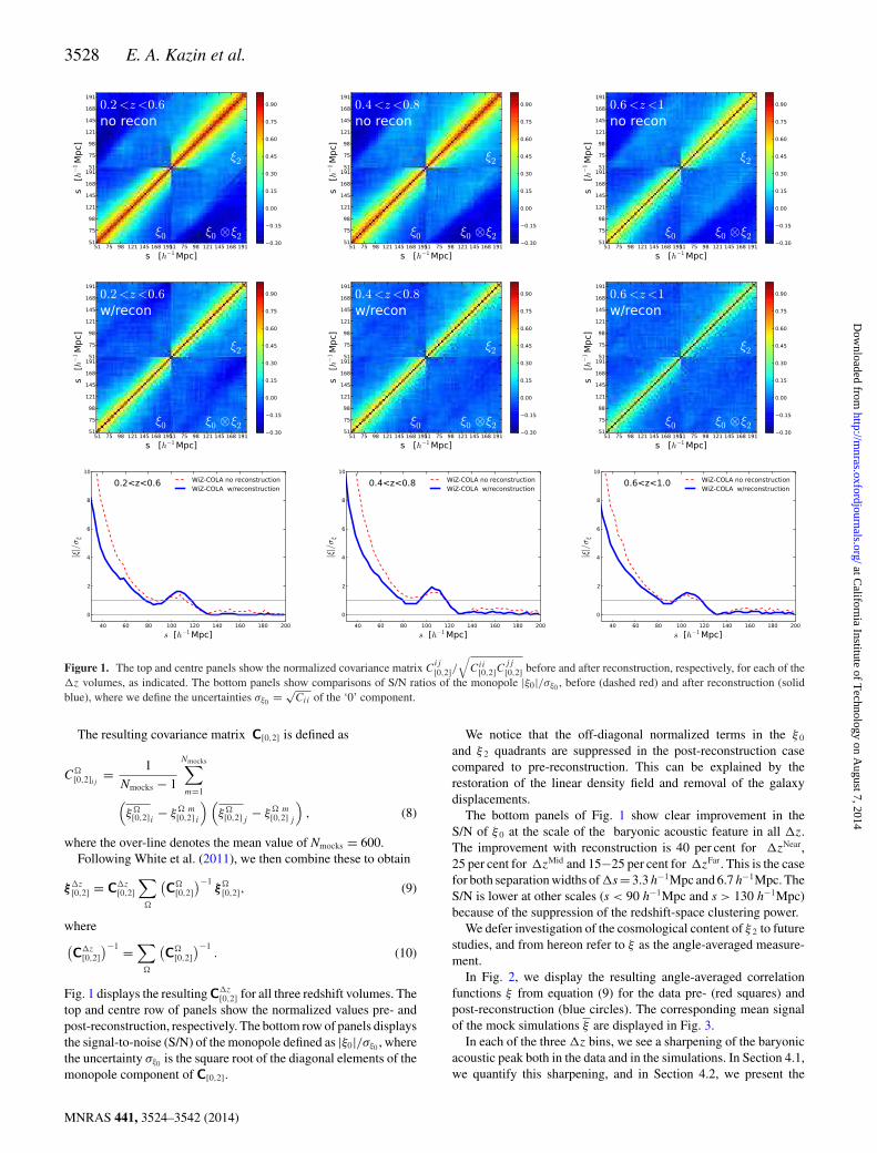
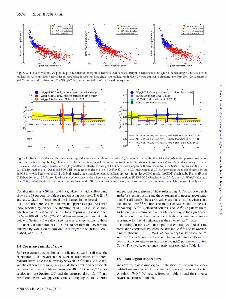
Figure 7. For each volume, we plot the post-reconstruction significance of detection of the baryonic acoustic feature against the resulting σα for each mockrealization. As in previous figures, the colour coding is such that blue circles are realizations in the >2σ subsample, red diamonds are from the <2σ subsample,and Xs do not yield a detection. The WiggleZ data points are indicated by the yellow squares.

Figure 8. Both panels display the volume-averaged distance to sound-horizon ratios DV/rs normalized by the fiducial value, where the post-reconstructionresults are indicated by the large blue circles. In the left-hand panel, the no reconstruction BAO-only results (red circles) and the ξ shape analysis results(Blake et al. 2011, orange squares) are slightly shifted for clarity. In the right-hand panel, we compare with two results from the SDSS-II (cyan star, 0.2 < z <

0.44; Padmanabhan et al. 2012) and SDSS-III (magenta triangles 0.2 < z < 0.43 0.43 < z < 0.7; Anderson et al. 2014a), as well as the result obtained by the6dFGS (z ∼ 0.1; Beutler et al. 2011). In both panels, the cosmology prediction lines are best-fitting flat �CDM results (�CDM) obtained by Planck (PlanckCollaboration et al. 2013a; solid) where the yellow band is the 68 per cent confidence region, SDSS-BOSS (Sanchez et al. 2013; dashed), WMAP (Komatsuet al. 2009; dot–dashed). The y-axis uncertainty bars are the 68 per cent confidence region, and those on the x-axis indicate the redshift range of analysis.

Collaboration et al. (2013a, solid line), where the wide yellow bandshows the 68 per cent confidence region using COSMOMC. The �m, hand wm ≡ �m h2 of each model are indicated in the legend.

Of the three predictions, our results appear to agree best withthose reported by Planck Collaboration et al. (2013a, solid line),which obtain h ∼ 0.67, where the local expansion rate is definedby H0 ≡ 100 h(km)(Mpc)−1(s)−1. When analysing various data setsbelow in Section 4.5 we show that our h results are similar to thoseof Planck Collaboration et al. (2013a) rather than the lower valueobtained by Wilkinson Microwave Anisotropy Probe (WMAP; dot–dashed) of h ∼ 0.71.

4.4 Covariance matrix of DV/rs

Before presenting cosmological implications, we first discuss thecalculation of the covariance between measurements in differentredshift slices. Due to the overlap between �zMid (0.4 < z < 0.8)and the other redshift bins, we calculate the correlation coefficientsbetween the α results obtained using the 300 stitched �zMid mockcatalogues (see Section 2.2) and the corresponding �zNear and�zFar catalogues. We apply the same α fitting algorithm as before

and present comparisons of the results in Fig. 9. The top two panelsare before reconstruction and the bottom panels are after reconstruc-tion. For all panels, the x-axis values are the α results when usingthe stitched �zMid volume, and the y-axis values are for the cor-responding �zNear (left-hand column) and �zFar (right) volumes.As before, we colour-code the results according to the significanceof detection of the baryonic acoustic feature, where the referencesubsample for this classification is the stitched �zMid case.

Focusing on the >2σ subsample in each case, we find that thecorrelation coefficient between the stitched �zMid and its overlap-ping neighbours is r ∼ 0.35−0.45. We verify that between �zNear

and �zFar r ∼ 0. We use these and the uncertainties in Table 3 toconstruct the covariance matrix of the WiggleZ post-reconstructionDV/rs. The inverse covariance matrix is presented in Table 4.

4.5 Cosmological implications

We next examine cosmological implications of the new distance–redshift measurements. In this analysis, we use the reconstructedWiggleZ DV(rfid

s /rs) results listed in Table 3, and their inversecovariance matrix (Table 4).

MNRAS 441, 3524–3542 (2014)




Dow

nloaded from



Figure 9. The top row shows the α distribution of the 300 mocks for the no reconstruction case and the bottom for post-reconstruction. In each, the x-axesvalues are those obtained with the �zMid (0.4 < z < 0.8) realizations, and the y-axes values are for �zNear (0.2 < z < 0.6; left-hand panels) and �zFar (0.6 <

z < 1; right-hand panels), accordingly. The blue circles are results of realizations in which the significance of detection of the baryonic acoustic feature afterreconstruction is better than 2σ , and the red diamonds are for mocks below this threshold, Xs indicate realizations with no detection. The correlation coefficientr for the >2σ subsample is indicated in the bottom left of each panel.

Our base model corresponds to an energy budget consisting ofbaryons (b), radiation (r), CDM and the so-called dark energy. Theprimordial density fluctuations are adiabatic and Gaussian with apower-law spectrum of Fourier amplitudes.

Table 4. The inverse covariance matrix of the DV(rfids /rs) measurements

from the reconstructed WiggleZ survey data. The volume-averaged distanceis defined in equation (14) and rs is the sound horizon at zdrag, and thefiducial cosmology assumed is given in Section 1. These measurementsare performed in three overlapping redshift slices 0.2 < z < 0.6, 0.4 <

z < 0.8, 0.6 < z < 1 with effective redshifts of 0.44, 0.6, 0.73 respectively.The data vector is DV(rfid

s /rs) =[1716.4, 2220.8, 2516.1] Mpc as listed inTable 3. As the matrix is symmetric we quote the upper diagonal, and forbrevity multiply by a factor of 104 Mpc2. That is, the user should multiplyeach element by this factor, e.g. the first element would be 2.1789887810−4 Mpc−2.

Redshift slice 0.2 < z < 0.6 0.4 < z < 0.8 0.6 < z < 1

0.2 < z < 0.6 2.178 988 78 −1.116 333 21 0.469 828 510.4 < z < 0.8 1.707 120 04 −0.718 471 550.6 < z < 1.0 1.652 831 75

We investigate four models. The first is the flat cosmological con-stant CDM paradigm, where the equation of state of dark energyis set to w = −1 (�CDM). We then relax the assumption of flat-ness (o�CDM). We also investigate the variation of w both whenassuming flatness (wCDM), as well as without (owCDM)

The main advantage of using information from low-redshift sur-veys z < 1 is their ability to constrain the equation of state of darkenergy w and the curvature �K, which are otherwise degeneratewhen analysing the CMB on its own. This is understood throughthe relationship between the expansion rate H(z) and the cosmiccomposition:

H (z)2 = H 20

(�M (1 + z)3 + �K (1 + z)2

+ �r (1 + z)4 + �DEe3∫ z

01+w(z′)

1+z′ dz′), (20)

where∑

i�i = 1 for i = m, K, r, DE. According to the definitionof DV (equation 14), our DV(rfid

s /rs) measurements yield degene-racies between H, DA and the sound horizon at the end of the dragepoch rs.

MNRAS 441, 3524–3542 (2014)




Dow

nloaded from



The physical angular diameter distance3

DA = 1

1 + z

c

H0

1√−�Ksin

(√−�K

χ

c/H0

)(21)

integrates over H through the definition of the comoving distance:

χ (z) = c

∫ z

0

dz′

H (z′). (22)

We calculate the sound horizon rs and the end-of-drag redshift zd

by using CAMB (Lewis et al. 2000). For our fiducial cosmology weobtain rfid

s =148.6 Mpc. We point out that another popular choice ofcalculating rs is by using equation 6 of Komatsu et al. (2009) and zd

with their equations 3– 5. With this we obtain rfids =152.3 Mpc. We

do not use this last calculation in our analysis. See Section 4.3 for adiscussion regarding these differences across other survey results.

Information from the CMB is required to break the degeneracywith the sound horizon scale rs. For this purpose, we use the PlanckCMB temperature anisotropies (Planck Collaboration et al. 2013b),and the CMB polarization measurements from WMAP9 (Bennettet al. 2013). When analysing the CMB information we vary thephysical baryon density wb ≡ �b h2, the physical CDM densitywc ≡ �c h2, the ratio of the sound horizon to the angular diameterdistance at the last-scattering surface �, the Thomson scatteringoptical depth due to reionization τ , the scalar power-law spectralindex ns and the log power of the primordial curvature perturbationln (1010As) (at k = 0.05 Mpc−1).

The CMB anisotropies also depend on the following parameters,which we fix: the sum of neutrino masses

∑mν =0.06eV, the ef-

fective number of neutrino-like relativistic degrees of freedom Neff

= 3.046, the fraction of baryonic mass in helium YP = 0.24, theamplitude of the lensing power relative to the fiducial value AL = 1.We also set to zero the effective mass of sterile neutrinos meff

ν, sterile,the tensor spectrum power-law index nt, the running of the spectralindex dns/d ln k and the ratio of tensor primordial power to curva-ture power r0.05. Planck Collaboration et al. (2013a) describe thenuisance parameters that are marginalized when fitting the CMBdata.

In addition, we use the 6dF Galaxy Survey (6dFGS) BAO mea-surement rs/DV = 0.336 ± 0.015 obtained by Beutler et al. (2011).Lastly, to quantify the improvements due to using the reconstructedWiggleZ DV(rfid

s /rs), we compare all results to those obtained whenusing the A(z) ∝ DV

√wM measurements of Blake et al. (2011).

They conclude that, when using the full shape of ξ as a standardruler, the A(z) parameter, as introduced by Eisenstein et al. (2005),is a more appropriate representation of the BAO information. Thevalues used here at z = 0.44, 0.6, 0.73 are listed in their table 5, andtheir inverse covariance matrix in their table 2.

We use the COSMOMC package (October 2013 version; Lewis et al.2002) to calculate the posteriors. The algorithm explores cosmo-logical parameter space by Monte Carlo sampling data sets whereit does accurate calculations of theoretical matter power spectrumand temperature anisotropy C� calculations using CAMB (Lewis et al.2000).

In our MCMC runs, we test the following combinations of data:

(i) CMB: Planck temperature fluctuations (Planck Collaborationet al. 2013b) and WMAP9 polarization (Bennett et al. 2013).

(ii) CMB+(WiggleZ pre-recon): CMB with the A(z) pre-reconstruction constraints from Blake et al. (2011).

3 Note that this is generic because isin (ix) = −sinh (x).

(iii) CMB+(WiggleZ post-recon): CMB with post-reconstruction DV(rfid

s /rs) results investigated here.(iv) CMB+(WiggleZ post-recon)+6dFGS: same as CMB+

(WiggleZ post-recon) with the addition of the baryonic acousticfeature results from the 6dFGS.

For comparison, we also test CMB with the 6dFGS results withoutinformation from WiggleZ.

Here, we report results for the local expansion rate H0, the den-sity of matter �m, the equation of state of dark energy w and thecurvature parameter �K, as relevant in the tested models.

Our results are summarized in Table 5 and in Fig. 10. All theresults show consistency with the flat (�K = 0) cosmological con-stant (w = −1) CDM paradigm. In the following subsections, wedescribe the main results of the four models tested.

4.5.1 �CDM results

The top-left panel of Fig. 10 presents the joint posterior probabilitydistribution of H0 and �m, and the marginalized results are summa-rized in Table 5. These measurements follow the degeneracy line ofconstant �m h3 (e.g. Percival et al. 2002; Sanchez et al. 2014). Allcombinations of data sets tested yield consistent results. There isa moderate improvement when adding the reconstructed WiggleZDV(rfid

s /rs) information to that of the CMB. This can be quanti-fied by the marginalized measurement of H0 improving from 1.8to 1.5 per cent accuracy, and �m from 5.4 to 4.7 per cent accuracy.Comparing CMB+(WiggleZ no recon) to the other combinations,we conclude that the reconstruction of WiggleZ and the additionalinformation from 6dFGS does little to improve the H0 and �m

measurements.

4.5.2 wCDM results

We now allow w to vary as a constant (i.e. no dependence on z). Thebottom-left panel of Fig. 10 presents the joint posterior probabilityof H0 and w. Here, we see that the CMB alone does not constrain thiscombination well, showing a large allowed range towards the lowerregion of w. Adding the pre-reconstruction WiggleZ informationdoes little to improve these measurements. Replacing with the post-reconstruction WiggleZ DV(rfid

s /rs), we see a slight improvementof the w measurement on its low side of the 68 per cent confidenceregion (but there is no improvement on the high side). A furthersubstantial improvement is achieved when adding information fromthe 6dFGS baryonic acoustic feature resulting in w = −1.08+0.15

−0.12,an ∼13 per cent accuracy measurement. This can be explained bythe fact that the low redshift DV/rs is particularly sensitive to H0,helping to break the degeneracy.

4.5.3 o�CDM results

When allowing for variation of �K and assuming w = −1, wenotice some improvement in constraints when adding the WiggleZpre-reconstruction to that of the CMB. When replacing the Wig-gleZ pre-reconstruction A(z) by the post-reconstruction DV(rfid

s /rs),however, we see substantial improvement in the measurements onthe high side of �K. Further improvement to measurements on thelow side of �K are obtained when adding information from the6dFGS baryonic acoustic feature. These are shown in the top-rightpanel of Fig. 10 which displays the joint posterior probability of H0

and �K.

MNRAS 441, 3524–3542 (2014)




Dow

nloaded from



Table 5. Constraints assuming flat �CDM.

Parameter/Data set(s) CMB CMB+(WiggleZ no-recon) CMB+(WiggleZ w/recon) CMB+(WiggleZ w/recon)+6dFGS

�CDM

H0 67.26+1.19−1.20 67.52+1.05

−1.03 67.00+1.02−1.03 67.15+0.99

−0.97

�m 0.316+0.016−0.018 0.312+0.014

−0.014 0.319+0.014−0.016 0.317+0.013

−0.015

−2ln (L) 9805.3 9805.2 9805.4 9804.9

wCDM

H0 83.36+14.70−7.29 81.15+9.67

−11.60 72.33+5.09−10.48 69.04+3.26

−4.01

�m 0.217+0.023−0.078 0.227+0.035

−0.074 0.285+0.067−0.059 0.304+0.030

−0.033

w −1.49+0.25−0.42 −1.44+0.33

−0.34 −1.18+0.36−0.19 −1.08+0.15

−0.12

�AIC 0.3 −0.1 −2.8 −2.6

o�CDM

H0 56.13+5.26−6.05 66.24+2.61

−2.60 64.92+2.03−2.05 65.84+1.69

−1.70

�m 0.462+0.072−0.107 0.324+0.024

−0.028 0.337+0.022−0.024 0.327+0.017

−0.019

100�K −3.83+2.91−1.78 −0.39+0.74

−0.66 −0.64+0.62−0.55 −0.43+0.47

−0.47

�AIC 0.5 −2.5 0.0 −2.7

owCDM

H0 61.24+9.28−21.01 80.26+9.41

−12.47 76.40+7.29−13.06 70.38+3.43

−4.55

�m 0.451+0.119−0.289 0.230+0.037

−0.079 0.255+0.057−0.080 0.289+0.032

−0.032

w −1.23+0.84−0.47 −1.55+0.44

−0.37 −1.50+0.51−0.33 −1.27+0.24

−0.18

100�K −4.18+4.23−1.55 −0.54+0.46

−0.47 −0.78+0.42−0.43 −0.83+0.44

−0.55

�AIC −0.8 −1.5 −1.4 −2.4

CMB refers to temperature fluctuations of Planck Collaboration et al. (2013b) and WMAP9 polarization (Bennett et al. 2013).WiggleZ no-recon refers to the pre-reconstruction A(z) obtained by using the full shape of ξ (Blake et al. 2011).WiggleZ w/recon refers to the post-reconstruction DV(rfid

s /rs) measurements presented here.6dFGS refers to the baryonic acoustic feature measurements of that survey (Beutler et al. 2011).In the �CDM section, we quote the maximum likelihood as −2ln L.In the wCDM, o�CDM, owCDM sections, we quote the �AIC ≡ AIC�CDM − AICM of each model M, as explained in the text. A positive�AIC indicates a preference for the model M over �CDM and vice versa. The relative likelihood of the model M can be quantified asexp(�AIC/2).

4.5.4 owCDM results

Lastly, we allow both w and �K to vary and find results to beconsistent with the flat cosmological constant paradigm. This isshown in the bottom-right panel of Fig. 10 which displays the jointposterior probability of these parameters. As expected, the CMB-only results do not constrain these parameters well, and the additionof the WiggleZ information yields substantial improvement. Asnoticed in the case of o�CDM case, we obtain a clear improvementin the higher end of the confidence region of �K when addingto the CMB the reconstructed WiggleZ DV(rfid

s /rs), compared toadding the pre-reconstruction A(z). The marginalized 68 per centconfidence region of �K is limited to [−0.0121,−0.0036].

Adding the baryonic acoustic feature from the 6dFGS does notimprove constraints on the curvature but does substantially reducethe allowed space for w, as seen in the wCDM case. In the caseof CMB+(WiggleZ post-recon)+6dFGS we obtain a marginalizedresult of w = −1.27+0.24

−0.18, a 17 per cent accuracy measurement.To better understand contributions from WiggleZ compared to

those from 6dF, when added to the CMB information, in the bottom-right panel of Fig. 10 we plot in yellow dashed constraints ob-tained with CMB+6dF without WiggleZ data. This result showsthat CMB+6dF alone is not enough to simultaneously constrain w

and �K. We do find in the o�CDM case, however, that CMB+6dF

constrains H0 and �K in a similar manner to results obtained usingCMB+(WiggleZ pre-recon).

As mentioned above, in all of our tests we find consistency with�CDM model. We now turn to quantify the model selection com-pared to �CDM. For this purpose, we use the Akaike informationcriterion, which incorporates trade-offs between the goodness offits to the additional complexity of each model (Akaike 1974). Foreach model M we quantify AICM ≡ 2p − 2 ln(L), where p is thenumber of parameters and L is the maximized value of the likeli-hood function. We then define �AIC ≡ AIC�CDM − AICM as ourindicator of the preferred model. A positive �AIC prefers model Mover �CDM and vice versa. The relative likelihood of the modelscan be quantified as exp(�AIC/2).

In Table 5, we list the �AIC of the models wCDM, o�CDM,owCDM, which should be read by column (for each data set combi-nation). We find non-positive values of �AIC values for all thedata sets which include BAO in all models, meaning that themodel that is preferred given the data (CMB, WiggleZ, 6dFGS)is �CDM. For example, when comparing the wCDM modelto �CDM and using the CMB+(WiggleZ w/recon) we obtain�AIC = −2.8, i.e. the relative likelihood of the wCDM modelis 0.247 times that of �CDM according to the Akaike informationcriteria.

MNRAS 441, 3524–3542 (2014)




Dow

nloaded from



Figure 10. Marginalized 68 and 95 per cent joint confidence regions of cosmological parameter pairs, as indicated. In the left-hand panels, we assume flatness,where the top-left panel is �CDM and the bottom left is wCDM, where w is the equation of state of dark energy. In the right-hand panels, we let the curvature�K vary, where the top-right panel is o�CDM and the bottom right is owCDM. The expansion rate H0 is in units of km s−1 Mpc−1 and �m is the matterdensity. In all panels, the dot–dashed green contours are when using information only from the CMB: Planck temperature fluctuations (Planck Collaborationet al. 2013b) and WMAP9 polarization (Bennett et al. 2013). CMB, WiggleZ pre-recon (dashed grey) is when adding A(z) information from the WiggleZ ξ

full-shape analysis (Blake et al. 2011). CMB, WiggleZ post-recon (solid blue) is when adding to CMB our post-reconstruction DV(rfids /rs) results. The CMB,

WiggleZ, 6dFGS results (dotted red) is when we add to CMB, WiggleZ post-recon BAO results from the 6dFGS (Beutler et al. 2011). For comparison, in thebottom right we also show results of CMB+6dFGS without WiggleZ information.

5 SU M M A RY

We present improved distance measurements in the redshift shiftrange 0.2 < z < 1 using the WiggleZ Dark Energy Survey galaxies,by applying the reconstruction of the baryonic acoustic featuretechnique, which utilizes additional information encoded in thedensity field.

The constraints on DV(rfids /rs) are 1716 ± 83 Mpc, 2221 ±

101 Mpc, 2516 ± 86 Mpc (68 per cent CL) for effective redshifts

zeff = 0.44, 0.6, 0.73, respectively. These results are model indepen-dent as we focus on the geometrical information contained in thebaryonic acoustic feature, and not the full shape of ξ .

Fig. 8 shows a comparison of WiggleZ DV/rs measurementsobtained by various methods with other data sets and cosmologi-cal predictions. The DV/rs measurements obtained by analysis ofthe baryonic acoustic feature position when using pre- and post-reconstruction data are shown to be consistent. Furthermore, these

MNRAS 441, 3524–3542 (2014)




Dow

nloaded from



results also agree with those obtained by Blake et al. (2011), whoused the full shape of the pre-reconstruction ξ as a standard ruler.

Interestingly, although we use a cosmology as predicted byWMAP as our fiducial, when converting redshifts to comoving dis-tances before counting the pairs of galaxies, the post-reconstructionDV/rs results show a preference for the distance–redshift pre-dictions of the best-fitting cosmologies measured by PlanckCollaboration et al. (2013a) and BOSS (e.g. Sanchez et al. 2013).

These 3.4–4.8 per cent accuracy post-reconstruction DV/rs

measurements represent a significant improvement from the pre-reconstruction case, and from the analysis of the full shape ofξ .4 These measurement improvements are effectively equivalentto those expected from surveys with up to 2.5 times the volumeof WiggleZ.5 To be conservative, here we assume a comparisonbetween our post-reconstruction BAO-only results to those of thepre-reconstruction ξ full-shape analysis reported by Blake et al.(2011).6

We test for sample variance by analysing 600 mock simulationsand find that reconstruction of the density field should yield a sharp-ened baryonic acoustic feature 65 per cent of the time, and ourDV(rfid

s /rs) results are within these expectations.The main limitations of the WiggleZ combined volumes are the

edge effects, completeness and large shot-noise. Although we showthat reconstruction successfully works on the data and most mocks,we find that it fails to yield an improved significance of detectionof the baryonic acoustic feature in ∼30–40 per cent of the cases,depending on the redshift range. We also find that 3–6 per cent ofthe mock realizations fail to detect a baryonic acoustic featurepost-reconstruction.

In Table 4, we provide the inverse covariance matrix of theDV(rfid

s /rs) measurements between these overlapping �z volumes,which can be used to calculate cosmological implications. We com-bine our measurements with CMB temperature anisotropies fromPlanck and CMB polarization of WMAP9, as well as the baryonicacoustic feature of the 6dFGS.

Using these post-reconstruction DV(rfids /rs) measurements, we

obtain consistent measurements of fundamental cosmological pa-rameters compared with those obtained when using the Blake et al.(2011) A(z) results. Assuming a curved CDM model while vary-ing the equation of state of dark energy, we find consistency withthe flat �CDM model. The significant improvement in measuringDV(rfid

s /rs), obtained by applying reconstruction, yields moderateimprovements on constraining �K (o�CDM, owCDM), and onlyslight improvement in w (wCDM, owCDM) and H0, �m (whenexamining the flat �CDM model).

Testing the �CDM model we obtain a marginalized constraintof H0 = 67.15 ± 0.98 km s−1 Mpc−1, which is in a 2.6σ tensionwith the SH0ES measurement of H0 = 73.8 ± 2.4 km s−1 Mpc(Riess et al. 2011).7 The density of matter is constrained in therange �m = 0.317 ± 0.014. Relaxing the assumption of flatnesswe constrain the curvature to �K = −0.0043 ± 0.0047. When

4 This statement is true for our analysis in the context of constraining DV/rs;the full shape of ξ contains more information, e.g. �m h2 and ns, which isnot investigated here.5 The calculation is based on squaring the uncertainty ratio, where we assumeσ 2

α ∝ 1/Volume.6 When comparing between BAO-only pre- and post-reconstruction the im-provement is effectively equivalent to surveys with volumes up to 4.7 largerthan WiggleZ.7 Calculation: (73.8−67.15)/

√2.42 + 0.982 = 2.6

assuming a flat wCDM model, the equation of state of dark energyis estimated to be wDE = −1.08 ± 0.135.

In the analysis of the cosmological constraints, we do not compareresults with those of the SDSS. Although the overlap between thesurveys is small, current investigation is underway to quantify thecovariance of the DV/rs measurements of the surveys (Beutler,Blake et al. in preparation).

To summarize we find that, although the reconstruction procedureis most effective in contiguous surveys, it can be applied success-fully in surveys that are patchy, that have high shot-noise and sig-nificant edge effects. This demonstrates the power of the techniquein producing a sharper baryonic acoustic feature from which wecan obtain significantly improved unbiased distance measurements.

AC K N OW L E D G E M E N T S

We thank Florian Beutler, Daniel Eisenstein, Shahab Joudaki,Antony Lewis, Felipe Marin and Ariel Sanchez for useful discus-sions. EK and JK are supported by the Australian Research Coun-cil Centre of Excellence for All-sky Astrophysics (CAASTRO),through project number CE110001020. CB acknowledges the sup-port of the Australian Research Council through the award of aFuture Fellowship. TMD acknowledges the support of the Aus-tralian Research Council through a Future Fellowship award,FT100100595. The numerical simulation was supported by theSwinSTAR supercomputer at Swinburne University of Technol-ogy and the Raijin supercomputer through the Flagship AllocationScheme of the NCI National Facility at the ANU.

R E F E R E N C E S

Akaike H., 1974, Ann. Stat., 19, 461Anderson L. et al., 2012, MNRAS, 427, 3435Anderson L. et al., 2014a, MNRAS, 441, 24Anderson L. et al., 2014b, MNRAS, 439, 83Angulo R. E., Baugh C. M., Frenk C. S., Lacey C. G., 2008, MNRAS, 383,

755Bennett C. L. et al., 2013, ApJS, 208, 20Bernardeau F., Colombi S., Gaztanaga E., Scoccimarro R., 2002, Phys. Rep.,

367, 1Beutler F. et al., 2011, MNRAS, 416, 3017Blake C., Glazebrook K., 2003, ApJ, 594, 665Blake C. et al., 2011, MNRAS, 418, 1707Blake C. et al., 2012, MNRAS, 425, 405Carlson J., White M., 2010, ApJS, 190, 311Crocce M., Scoccimarro R., 2008, Phys. Rev. D, 77, 023533Drinkwater M. J. et al., 2010, MNRAS, 401, 1429Eisenstein D. J., Hu W., 1998, ApJ, 496, 605Eisenstein D. J. et al., 2001, AJ, 122, 2267Eisenstein D. J. et al., 2005, ApJ, 633, 560Eisenstein D. J., Seo H.-J., Sirko E., Spergel D. N., 2007, ApJ, 664, 675Feldman H. A., Kaiser N., Peacock J. A., 1994, ApJ, 426, 23Hartlap J., Simon P., Schneider P., 2007, A&A, 464, 399Hoffman Y., Ribak E., 1991, ApJ, 380, L5Hogg D. W., 1999, preprint (astro-ph/9905116)Kazin E. A., Sanchez A. G., Blanton M. R., 2012, MNRAS, 419, 3223Kazin E. A. et al., 2013, MNRAS, 435, 64Kim J., Park C., Gott J. R., III, Dubinski J., 2009, ApJ, 701, 1547Komatsu E. et al., 2009, ApJS, 180, 330Landy S. D., Szalay A. S., 1993, ApJ, 412, 64Lewis A., Challinor A., Lasenby A., 2000, Astrophys. J., 538, 473Lewis I. et al., 2002, MNRAS, 334, 673Manera M. et al., 2013, MNRAS, 428, 1036Mehta K. T., Seo H.-J., Eckel J., Eisenstein D. J., Metchnik M., Pinto P.,

Xu X., 2011, ApJ, 734, 94

MNRAS 441, 3524–3542 (2014)




Dow

nloaded from

http://arxiv.org/abs/astro-ph/9905116



Mehta K. T., Cuesta A. J., Xu X., Eisenstein D. J., Padmanabhan N., 2012,MNRAS, 427, 2168

Meiksin A., White M., Peacock J. A., 1999, MNRAS, 304, 851Noh Y., White M., Padmanabhan N., 2009, Phys. Rev. D, 80, 123501Padmanabhan N., White M., Cohn J. D., 2009, Phys. Rev. D, 79, 63523Padmanabhan N., Xu X., Eisenstein D. J., Scalzo R., Cuesta A. J., Mehta

K. T., Kazin E., 2012, MNRAS, 427, 2132Peebles P. J. E., Yu J. T., 1970, ApJ, 162, 815Percival W. J. et al., 2002, MNRAS, 337, 1068Perlmutter S. et al., 1999, ApJ, 517, 565Planck Collaboration et al., 2013a, preprint (arXiv:1303.5076P)Planck Collaboration et al., 2013b, preprint (arXiv:1303.5075P)Riess A. G. et al., 1998, AJ, 116, 1009Riess A. G. et al., 2011, ApJ, 730, 119Sanchez A. G., Baugh C. M., Angulo R., 2008, MNRAS, 390, 1470Sanchez A. G., Crocce M., Cabre A., Baugh C. M., Gaztanaga E., 2009,

MNRAS, 400, 1643Sanchez A. G. et al., 2012, MNRAS, 425, 415Sanchez A. G. et al., 2013, MNRAS, 433, 1202Sanchez A. G. et al., 2014, MNRAS, 440, 2692Seo H.-J., Eisenstein D. J., 2003, ApJ, 598, 720Seo H.-J., Eisenstein D. J., 2007, ApJ, 665, 14Seo H.-J., Siegel E. R., Eisenstein D. J., White M., 2008, AJ, 686, 13Seo H. et al., 2010, ApJ, 720, 1650Smith R. E., Scoccimarro R., Sheth R. K., 2008, Phys. Rev. D, 77, 043525Taruya A., Saito S., Nishimichi T., 2011, Phys. Rev. D, 83, 103527Tassev S., Zaldarriaga M., Eisenstein D. J., 2013, J. Cosmol. Astropart.

Phys., 6, 36White M. et al., 2011, ApJ, 728, 126Xu X., Padmanabhan N., Eisenstein D. J., Mehta K. T., Cuesta A. J., 2012,

MNRAS, 427, 2146York D. G. et al., 2000, AJ, 120, 1579Zel’dovich Y. B., 1970, A&A, 5, 84

1Centre for Astrophysics and Supercomputing, Swinburne University ofTechnology, PO Box 218, Hawthorn, VIC 3122, Australia2ARC Centre of Excellence for All-sky Astrophysics (CAASTRO), 44 RosehillStreet, Redfern, NSW 2016, Australia

3Department of Physics, Yale University, 260 Whitney Ave, New Haven, CT06520, USA4Australian Astronomical Observatory, PO Box 915, North Ryde, NSW 1670,Australia5Carnegie Institution of Washington, Las Campanas Observatory, Colina elPino s/n, Casilla 601, Chile6Sydney Institute for Astronomy, School of Physics, University of Sydney,NSW 2006, Australia7School of Mathematics and Physics, University of Queensland, Brisbane,QLD 4072, Australia8California Institute of Technology, MC 278-17, 1200 East California Boule-vard, Pasadena, CA 91125, USA9South African Astronomical Observatory, PO Box 9, Observatory 7935,South Africa10Department of Astronomy and Astrophysics, University of Chicago, 5640South Ellis Avenue, Chicago, IL 60637, USA11Australia Telescope National Facility, CSIRO, Epping, NSW 1710,Australia12Department of Astronomy and Astrophysics, University of Toronto, 50 StGeorge Street, Toronto, ON M5S 3H4, Canada13Observatories of the Carnegie Institute of Washington, 813 Santa BarbaraSt, Pasadena, CA 91101, USA14School of Physics, Monash University, Clayton, VIC 3800, Australia15Department of Physics and Mathematics, University of Hull, CottinghamRoad, Hull HU6 7RX, UK16School of Physics, University of Melbourne, Parksville, VIC 3010,Australia17Research School of Astronomy and Astrophysics, Australian National Uni-versity, Weston Creek, ACT 2600, Australia18Max Planck Institut fur extraterrestrische Physik, Giessenbachstraβe,D-85748 Garching, Germany19Department of Physics and Astronomy, University of British Columbia,6224 Agricultural Road, Vancouver, BC V6T 1Z1, Canada

This paper has been typeset from a TEX/LATEX file prepared by the author.

MNRAS 441, 3524–3542 (2014)




Dow

nloaded from

http://arxiv.org/abs/1303.5076

http://arxiv.org/abs/1303.5075


The WiggleZ Dark Energy Survey: improved distance ...

Documents

Transcript of The WiggleZ Dark Energy Survey: improved distance ...