The Wiener index of a graph - TU Graz
86
Nina Sabine SCHMUCK The Wiener index of a graph DIPLOMA THESIS written to obtain the academic degree of a Diplom-Ingenieurin Diplomstudium Technische Mathematik Graz University of Technology Graz University of Technology Supervisor: Gast-Prof. Dipl.-Ing. Dr.techn. Stephan WAGNER Institut f¨ ur Mathematik A Graz, August 2010
Transcript of The Wiener index of a graph - TU Graz

Nina Sabine SCHMUCK
The Wiener index of a graph
DIPLOMA THESIS
written to obtain the academic degree of a Diplom-Ingenieurin
Diplomstudium Technische Mathematik
Graz University of Technology
Graz University of Technology
Supervisor:Gast-Prof. Dipl.-Ing. Dr.techn. Stephan WAGNER
Institut fur Mathematik A
Graz, August 2010

Statutory Declaration
I declare that I have authored this thesis independently, that I have not used other thanthe declared sources/resources, and that I have explicitly marked all material which hasbeen quoted either literally or by content from the used sources.
. . . . . . . . . . . . . . . . . . . . . . . . . . . . . . . . . . .date
. . . . . . . . . . . . . . . . . . . . . . . . . . . . . . . . . . . . . . . . . . . .(signature)

Contents
1 Introduction - Basic notations and definitions 6
2 Different ways to compute the Wiener index of trees 92.1 Direct formulas . . . . . . . . . . . . . . . . . . . . . . . . . . . . . . . . . 9
2.1.1 Branching points, segments and the Wiener index . . . . . . . . . . 132.1.2 Laplacian Eigenvalues and their influence on the Wiener index . . . 19
2.2 Recursive formulas . . . . . . . . . . . . . . . . . . . . . . . . . . . . . . . 242.2.1 The Wiener index of a thorn tree . . . . . . . . . . . . . . . . . . . 322.2.2 A k-subdivision of a tree and its Wiener index . . . . . . . . . . . . 37
3 Lower and upper bounds 403.1 Bounds for general graphs . . . . . . . . . . . . . . . . . . . . . . . . . . . 403.2 Bounds for trees . . . . . . . . . . . . . . . . . . . . . . . . . . . . . . . . . 42
3.2.1 Trees with given maximum degree . . . . . . . . . . . . . . . . . . . 423.2.2 Trees with given degree sequence . . . . . . . . . . . . . . . . . . . 51
4 Inverse problems - forbidden values 714.1 Connected graphs . . . . . . . . . . . . . . . . . . . . . . . . . . . . . . . . 714.2 Bipartite graphs . . . . . . . . . . . . . . . . . . . . . . . . . . . . . . . . . 724.3 Trees . . . . . . . . . . . . . . . . . . . . . . . . . . . . . . . . . . . . . . . 79
3

Preface
The first investigations into the Wiener index were made by Harold Wiener in 1947 whorealized that there are correlations between the boiling points of paraffin and the structureof the molecules (see [23]). In particular, he mentions in his article that the boiling pointtB can be quite closely approximated by the formula
tB = aw + bp+ c,
where w is the Wiener index, p the polarity number and a, b and c are constants for agiven isomeric group. Since then it has become one of the most frequently used topologicalindices in chemistry, as molecules are usually modelled as undirected graphs, especiallytrees. For example, in the drug design process, the aim is the construction of chemicalcompounds with certain properties, which not only depend on the chemical formula butalso strongly on the molecular structure, as one can easily see when considering cocaineand scopolamine, both having the chemical formula C17H21NO4.
Furthermore, there are many situations in communication, facility location, cryptology,architecture etc. where the Wiener index of the corresponding graph or the average dis-tance is of great interest. One of these problems, for example, is to find a spanning treewith minimum average distance.
In the first chapter we define the Wiener index and some properties of graphs, par-ticularly trees, that we will require later on. The second chapter deals with a variety offormulas for computing the Wiener index of trees. Some of those formulas can also beapplied to connected graphs.
Since calculating the Wiener index of a graph can be computationally expensive, wegive some cheaply computable lower and upper bounds for the Wiener index – given certaingraph properties – in chapter 3. In particular, we focus on trees with further constraints,such as a given maximum degree or degree sequence.
Finally, in chapter 4, we consider the inverse problem – Which numbers are Wienerindices? – for a number of classes of graphs and trees.
4

PREFACE 5
I want to thank all who helped me during my study of mathematics and the writingof my diploma thesis, especially Gast-Prof. Dr. Stephan Wagner and Ao.Univ.-Prof. Dr.Clemens Heuberger. Finally, I also want to thank my family for their support and Berndand Doris Haug for their linguistic advice.
Graz, August 2010
Nina Sabine Schmuck

Chapter 1
Introduction - Basic notations anddefinitions
Throughout the whole diploma thesis, all graphs will be finite, simple, connected andundirected, and in most cases we will consider trees.
Definition 1.1. Let G be a graph with vertex set V (G) and edge set E(G). The distancedG(u, v) between two vertices u, v ∈ V (G) is the minimum number of edges on a path inG between u and v.
Definition 1.2. Let G be as before. The Wiener index W (G) of G is defined by
W (G) =∑
{u,v}⊆V (G)
dG(u, v)
and the average distance µ(G) between the vertices of G by
µ(G) =W (G)(|V (G)|
2
) .Definition 1.3. Let G be as before. The distance dG(v) of a vertex v is the sum of alldistances between v and all other vertices of G.
Thus, one can define the Wiener index also in a slightly different way:
W (G) =1
2
∑v∈V (G)
dG(v) ,
where 12
compensates for the fact that each path between u and v is counted in dG(u) aswell as in dG(v).
Definition 1.4. Let G be a graph. The diameter d(G) of G is defined as
d(G) = min{u,v}⊆V (G)
dG(u, v).
6

CHAPTER 1. INTRODUCTION - BASIC NOTATIONS AND DEFINITIONS 7
Definition 1.5. The degree degG(v) of a vertex v ∈ V (G) is the number of edges incidentto v.
The degree sequence of G is a vector (degG(v1), degG(v2), . . . , degG(vn)) with degG(v1) ≥degG(v2) ≥ · · · ≥ degG(vn) and n = |V (G)|.
Furthermore we will need the following definitions:
Definition 1.6. Let T be a tree. A vertex v ∈ V (T ) is called branching point of T , ifdegT (v) ≥ 3. If degT (v) = 1, the vertex v is named leaf of T .
The path with n vertices, of which exactly 2 are leaves, is written as Pn, and the starwith exactly n− 1 leaves and 1 branching point is denoted by Sn.
Remark 1.1. It is easy to see that every tree on n vertices has at least 2 leaves and atmost n−2
2branching points.
Remark 1.2. As we will need the Wiener index of both the path and the star on severaloccasions, we compute their Wiener index in advance:
W (Sn) = n− 1︸ ︷︷ ︸branching point to leaves
+ 2n−2∑i=1
i︸ ︷︷ ︸between all pairs of leaves
= (n− 1)2,
W (Pn) =n∑i=1
i−1∑j=1
j =n∑i=1
(i
2
)=
(n+ 1
3
).
The last equation can be easily shown by induction.
Definition 1.7. Let T be a tree. A segment S of T is a path-subtree whose terminalvertices are branching points or leaves and internal vertices v have degree degT (v) = 2.The length of a segment S is equal to the number of edges in S and is denoted by lS. Theset of all vertices being terminal vertices of a segment is named by SP(T ). Moreover letS∗ be a subpath of S containing lS vertices, i.e. S∗ = S\{v} where v is a terminal vertexof S, and let S0 be S without both its terminal vertices.
Remark 1.3. Since each edge of a tree T on n vertices is used in exactly one segment, itis clear that ∑
S seg. of T
lS = n− 1.
To illustrate the above definitions let us examine the following two short examples:
Example 1.4. Let G be the graph shown in Figure 1.1. The distance e.g. between v4
and v6 is dG(v4, v6) = 2 using the path (v4, v7, v6), and the distance e.g. of v1 is dG(v1) =1 + 2 + 3 + 4 + 2 + 3 + 4 = 19. The Wiener index of G can be computed as follows:
W (G) =7∑i=1
8∑j=i+1
dG(vi, vj)

CHAPTER 1. INTRODUCTION - BASIC NOTATIONS AND DEFINITIONS 8
v1 v2 v3 v4 v5
v6 v7
v8
Figure 1.1: A graph G used in Example 1.4.
= (1 + 2 + 3 + 4 + 2 + 3 + 4) + (1 + 2 + 3 + 1 + 2 + 3)+
+ (1 + 2 + 1 + 2 + 2) + (1 + 2 + 1 + 1)+
+ (3 + 2 + 2) + (1 + 3) + 2
= 57.
Thus the average distance of G is
µ(G) =57(82
) =57
28≈ 2.0357.
Furthermore the degree sequence of G is (4, 3, 3, 3, 2, 1, 1, 1).
v1 v2 v3 v4 v5 v6
v7 v8 v9 v10 v11
v12
v13
Figure 1.2: A tree T used in Example 1.5.
Example 1.5. Now let us consider the tree T as shown in Figure 1.2. For example v1 isa leaf and v2 a branching point, but notice that v9 is neither a leaf nor a branching pointsince degT (v9) = 2.
A segment of T is e.g. S1 = (v2, v9, v12) with length lS1 = 2. Furthermore S∗1 can eitherbe the path (v2, v9) or the path (v9, v12), and S0
1 is the path only containing the vertex v9.Another segment would be S2 = (v3, v13) with S∗2 either (v3) or (v13) and S0
2 empty.

Chapter 2
Different ways to compute theWiener index of trees
As the path and therefore the distance between two vertices of a tree is unique, the Wienerindex of a tree is much easier to compute than that of an arbitrary graph. In the following,we will show different formulas for computing the Wiener index, in the first part directones and in the second part recursive ones that require certain characteristics of the treesbut in case their requirements are satisfied may make the calculation of the Wiener indexeasier by far.
2.1 Direct formulas
The first formula we are going to show is a very basic one and was found by H. Wiener in1947 (see [23]). While the definition of the Wiener index puts its stress on how far one hasto go from each vertex to reach all other vertices, this formula counts how often one hasto pass each edge.
Definition 2.1. Let e = (u, v) ∈ E(T ) be an edge of the tree T . The subtrees Tu and Tvare defined as the connected components of T containing u and v, respectively. The orderof the subtrees is denoted by nu(e) = |V (Tu)| and nv(e) = |V (Tv)|.
Theorem 2.1. Let T be a tree. Then
W (T ) =∑
e=(u,v)∈E(T )
nu(e)nv(e). (2.1)
Proof. As T is a tree, the unique path between a vertex x ∈ V (Tu) and a vertex y ∈ V (Tv)must contain e. If x and y are chosen in a different way, e is not part of the path betweenthem. Therefore nu(e)nv(e) is exactly the number of times how often e belongs to a pathbetween two vertices of T . Then the sum of nu(e)nv(e) over all edges of T must be theWiener index of T .
9
CHAPTER 2. DIFFERENT WAYS TO COMPUTE... 10
Remark 2.2. Dobrynin and Gutman give another proof of Theorem 2.1 in a more generalway in [6]. In addition to that they show for what types of graphs equation (2.1) holds andthat for all other cases the right-hand side of equation 2.1, which is denoted as the newgraph invariant W ∗ called Szeged index, is greater than the corresponding Wiener index.To be able to define W ∗ one has to generalize the definition of Tu and Tv first, which weare going to show in the following definition to give an idea of this closely related graphinvariant before continuing with our original topic.
Definition 2.2. Let e = (u, v) ∈ E(G) be an edge of the graph G. The sets Bu(e) andBv(e) of vertices of G are defined as
Bu(e) = {x ∈ V (G) : dG(x, u) < dG(x, v)}
Bv(e) = {y ∈ V (G) : dG(y, v) < dG(y, u)}.
The cardinalities of the sets are denoted by nu(e) = |Bu(e)| and nv(e) = |Bv(e)|.
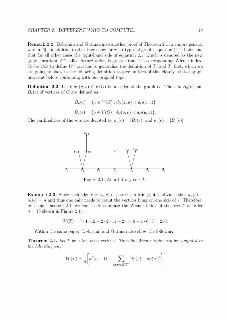
v1 v2 v3 v4 v5 v6 v7
v8 v9v10 v11 v12
v13
Figure 2.1: An arbitrary tree T .
Example 2.3. Since each edge e = (u, v) of a tree is a bridge, it is obvious that nu(e) +nv(e) = n and thus one only needs to count the vertices lying on one side of e. Therefore,by using Theorem 2.1, we can easily compute the Wiener index of the tree T of ordern = 13 shown in Figure 2.1:
W (T ) = 7 · 1 · 12 + 2 · 2 · 11 + 2 · 5 · 8 + 1 · 6 · 7 = 250.
Within the same paper, Dobrynin and Gutman also show the following:
Theorem 2.4. Let T be a tree on n vertices. Then the Wiener index can be computed inthe following way:
W (T ) =1
4
[n2(n− 1)−
∑(u,v)∈E(T )
[dT (v)− dT (u)]2].

CHAPTER 2. DIFFERENT WAYS TO COMPUTE... 11
Proof. As mentioned in Example 2.3, n = nu(e) + nv(e) for all edges e = (u, v). Furtherwe obtain
dT (v)− dT (u) =
( ∑x∈Bu(e)
dT (v, x) +∑
y∈Bv(e)
dT (v, y)
)
−( ∑x∈Bu(e)
dT (u, x) +∑
y∈Bv(e)
dT (u, y)
)=
∑x∈Bu(e)
(dT (v, x)− dT (u, x))−∑
y∈Bv(e)
(dT (u, y)− dT (v, y))
=∑
x∈Bu(e)
1−∑
y∈Bv(e)
1
= nu(e)− nv(e).
Thus together we obtain 2nu(e) = n+ (dT (v)− dT (u)) and 2nv(e) = n− (dT (v)− dT (u)).Substituting this into equation (2.1) we get
W (T ) =∑
(u,v)∈E(T )
1
2(n+ dT (v)− dT (u))
1
2(n− dT (v) + dT (u))
=1
4
∑(u,v)∈E(T )
[n2 − (dT (v)− dT (u))2
]=
1
4
[n2(n− 1)−
∑(u,v)∈E(T )
(dT (v)− dT (u))2
],
which completes the proof.
Example 2.5. Let T again be the tree in Figure 2.1. To apply Theorem 2.4 we make useof the fact that
dT (v)− dT (u) = nu(e)− nv(e)
for all edges e = (u, v) as we showed within the proof of Theorem 2.4. This simplifies thecalculation by far and we obtain
W (T ) =1
4[132 · 12− (7 · 112 + 2 · 92 + 2 · 32 + 12)] = 250.
Corollary 2.6. Let T be a tree on n vertices. Then
W (T ) =1
4
[n(n− 1) +
∑v∈V (T )
degT (v)dT (v)
].

CHAPTER 2. DIFFERENT WAYS TO COMPUTE... 12
v
u1
T1
u2
T2
um
Tm
Figure 2.2: Tree with branching point v and subtrees Ti, where m = degT (v)
Proof. Let N(v) be the set of all neighbours of the vertex v in T . It is obvious that|N(v)| = degT (v). Then we can rewrite the sum in Theorem 2.4 as follows
W (T ) =1
4
[n2(n− 1)−
∑(u,v)∈E(T )
[dT (v)− dT (u)]2]
=1
4
[n2(n− 1)− 1
2
∑v∈V (T )
∑u∈N(v)
(dT (v)2 − 2dT (v)dT (u) + dT (u)2)
]
=1
4
[n2(n− 1)− 1
2
∑v∈V (T )
(dT (v)2 degT (v)
− 2∑
u∈N(v)
dT (v)dT (u) + dT (v)2 degT (v))]
=1
4
[n2(n− 1)−
∑v∈V (T )
dT (v)(dT (v) degT (v)−
∑u∈N(v)
dT (u))].
To compute dT (ui) with ui ∈ N(v) we choose the path ui → v → x for every x ∈ V (T ).Now we counted two edges too many for each vertex in Ti, where Ti is defined as theconnected component of T including ui after deleting v (as shown in Figure 2.2). Thereforewe get
dT (ui) = n+ dT (v)− 2|Ti|,and altogether we obtain∑
u∈N(v)
dT (u) = degT (v)n+ dT (v) degT (v)− 2(n− 1).
Substituting this into W (T ) leads to
W (T ) =1
4
[n2(n− 1)−
∑v∈V (T )
(2(n− 1)dT (v)− ndT (v) degT (v))
]
=1
4
[n2(n− 1)− 4(n− 1)W (T ) + n
∑v∈V (T )
dT (v) degT (v)
].
Solving the equation for W (T ) leads to the desired statement.

CHAPTER 2. DIFFERENT WAYS TO COMPUTE... 13
Example 2.7. Now we apply Corollary 2.6 to the tree T of Figure 2.1:
W (T ) =1
4[13 · 12 + (1 · 42 + 4 · 31 + 2 · 28 + 3 · 27 + 4 · 30 + 2 · 39 + 1 · 50
+ 1 · 42 + 2 · 40 + 1 · 38 + 1 · 41 + 1 · 41 + 1 · 51)] = 250.
Remark 2.8. Examples 2.5 and 2.7 illustrate quite well that the formulas used there aremore of theoretical than of practical interest.
2.1.1 Branching points, segments and the Wiener index
Another very important formula is given by Doyle and Graver in [7]. But at first, we needthe following definition:
Definition 2.3. Let G be a connected graph. The vertices v1, v2, v3 ∈ V (G) are calledcollinear if there exists an ordering of the three vertices such that
dG(vi, vj) + dG(vj, vk) = dG(vi, vk).
The number of 3-subsets of V (G) which are not collinear is denoted by τ(G).
Theorem 2.9 (Doyle-Graver formula). Let T be a tree of order n. Then
W (T ) =
(n+ 1
3
)−∑
v∈V (T )
∑1≤i<j<k≤degT (v)
|V (Ti)| |V (Tj)| |V (Tk)| (2.2)
with Tl defined as in the proof of Corollary 2.6.
Proof. Let C be the set of all collinear 3-subsets of V (T ). As the path between twovertices u and v is unique, the only vertices w being collinear with u and v, such thatdT (u,w) + dT (w, v) = dT (u, v), are the vertices on the path between u and v. This meansthat for each pair u and v there exists exactly dT (u, v)− 1 vertices that are collinear withthem in this manner. Therefore we get
|C| =∑
{u,v}⊆V (T )
(dT (u, v)− 1) = W (T )−(n
2
).
Since all vertices u, v, w can be either collinear or non-collinear, we obtain
|C|+ τ(T ) =
(n
3
).
Combining these two formulas leads to
W (T ) =
(n
3
)+
(n
2
)− τ(T ) =
(n+ 1
3
)− τ(T ). (2.3)

CHAPTER 2. DIFFERENT WAYS TO COMPUTE... 14
Now, considering three non-collinear vertices u1, u2, u3 it is obvious that there mustexist a vertex v such that v lies on the paths between each pair of u1, u2, u3. Count-ing the number of non-collinear 3-subsets of V (T ) with v on their paths we get exactly∑
1≤i<j<k≤degT (v) |V (Ti)| |V (Tj)| |V (Tk)|. Thus
τ(T ) =∑
v∈V (T )
∑1≤i<j<k≤degT (v)
|V (Ti)| |V (Tj)| |V (Tk)|.
Substituting this into equation (2.3) completes the proof.
Remark 2.10. Notice that the first summation in equation (2.2) actually goes just over allbranching points of T . Furthermore notice that the first term in equation (2.2) is exactlythe Wiener index of the path of length n.
Example 2.11. The tree T shown in Figure 2.1 has the three branching points v2, v4
and v5. Since degT (v4) = 3, the vertex v4 contributes just one addend to the Doyle-Graver formula, whereas both v2 and v5, have degree 4, which leads to
(43
)= 4 different
combinations of their subtrees. This leads to the Wiener index
W (T ) =
(14
3
)− [1 · 1 · 2 + 1 · 1 · 8 + 1 · 2 · 8 + 1 · 2 · 8︸ ︷︷ ︸
obtained from v2
+ 6 · 1 · 5︸ ︷︷ ︸obtained from v4
+ 8 · 1 · 1 + 8 · 1 · 2 + 8 · 1 · 2 + 1 · 1 · 2︸ ︷︷ ︸obtained from v5
] = 250,
which is once again the same number.
On the following pages some further formulas based on either branching points orsegments are examined (see [4]).
Theorem 2.12. Let T be a tree on n vertices. Then
W (T ) =∑
S seg. of T
n1(S)nlS+1(S)lS +1
6
∑S seg. of T
lS(lS − 1)(3n− 2lS + 1) (2.4)
where n1(S) and nlS+1(S) are the number of vertices of the two connected componentsobtained by deleting all internal vertices of S and the corresponding edges (compare Defi-nition 2.1).
Proof. In order to prove this theorem we use formula (2.1) and rewrite it in terms ofsegments. Let S = (v1, v2, . . . , vlS , vlS+1) be a segment of T and ei = (vi, vi+1). Then weobtain nvi
(ei) = n1(S) + (i− 1) and nvi+1(ei) = nlS+1(S) + (lS− i) for i ∈ {1, 2, . . . , lS} and
clearly n1(S) + nlS+1(S) + lS − 1 = n. Thus the contribution of the edges of S to W (T ) is
lS∑i=1
nvi(ei)nvi+1
(ei) =
lS∑i=1
(n1(S) + i− 1)(nlS+1(S) + lS − i)

CHAPTER 2. DIFFERENT WAYS TO COMPUTE... 15
=
lS∑i=1
[n1(S)nlS+1(S) + (n1(S)− 1)lS − nlS+1(S)
+ (nlS+1(S)− n1(S) + lS + 1)i− i2]
= lSn1(S)nlS+1(S) + (n1(S)− 1)l2S − nlS+1(S)lS
+ (nlS+1(S)− n1(S) + lS + 1)lS(lS + 1)
2− lS(lS + 1)(2lS + 1)
6
= lSn1(S)nlS+1(S) +1
2(n1(S) + nlS+1(S) + lS − 1)l2S
+1
2(−n1(S)− nlS+1(S)− lS + 1 + 2lS)lS −
1
6(2l2S + 3lS + 1)lS
= lSn1(S)nlS+1(S) +1
2nl2S +
1
2(−n+ 2lS)lS −
1
6(2l2S + 3lS + 1)lS
= lSn1(S)nlS+1(S) +1
6lS(3nlS − 3n− 2l2S + 3lS − 1).
Summing this over all segments of T leads to the desired equation.
Example 2.13. The tree shown in Figure 2.1 has nine segments. As the segmentsS1 = (v1, v2), S2 = (v2, v8), S3 = (v4, v10), S4 = (v5, v11) and S5 = (v5, v12) are equiva-lent according to their length lSi
and the number of vertices n1(Si) and nlSi+1(Si), we get
n1(Si)nlSi+1(Si)lSi
= 12 for i = 1, . . . , 5. In the same manner we obtain for both segmentsS6 = (v2, v9, v13) and S7 = (v5, v6, v7) that the term n1(S)nlS+1(S)lS is 22. Further-more we have n1(S8)nlS8
+1(S8)lS8 = 40 for S8 = (v4, v5) and n1(S9)nlS9+1(S9)lS9 = 70 for
S9 = (v2, v3, v4). Thus according to equation (2.4) we obtain
W (T ) = 5 · 12 + 2 · 22 + 40 + 70 +1
6· 3 · [2 · 1 · (3 · 13− 2 · 2 + 1)] = 250.
Theorem 2.14. Let T be a tree of order n. Then the Wiener index can be computed by
W (T ) =1
12
[(3n2 + 1)(n− 1)− 3
∑S seg. of T
1
lS[dT (v1)− dT (vlS+1)]2 −
∑S seg. of T
l3S
]with v1 and vlS+1 being the terminal vertices of S.
Proof. In order to apply equation (2.4) we have to further investigate the productn1(S)nlS+1(S). Let T1(S) and TlS+1(S) with n1(S) and nlS+1(S) vertices, respectively,be the two connected subtrees obtained by deleting all inner vertices of S. Thus we get
dT (v1)− dT (vlS+1) =∑
x∈T1(S)
(dT (v1, x)− dT (vlS+1, x))
+∑
y∈TlS+1(S)
(dT (v1, x)− dT (vlS+1, x))

CHAPTER 2. DIFFERENT WAYS TO COMPUTE... 16
=∑
x∈T1(S)
(−lS) +∑
y∈TlS+1(S)
lS
= lS[nlS+1(S)− n1(S)].
Furthermore we know that n1(S) + nlS+1(S) = n− lS + 1. Together we obtain
n1(S)nlS+1(S) =1
4([n1(S) + nlS+1(S)]2 − [n1(S)− nlS+1(S)]2)
=1
4
[(n− lS + 1)2 − [dT (v1)− dT (vlS+1)]2
l2S
]and substituting this into equation (2.4) leads to
W (T ) =1
4
∑S seg. of T
(n− lS + 1)2lS −1
4
∑S seg. of T
1
lS[dT (v1)− dT (vlS+1)]2
+1
6
∑S seg. of T
lS(lS − 1)(3n− 2lS + 1)
=1
12
[∑S
(3n2 + 1)lS −∑S
l3S − 3∑S
1
lS[dT (v1)− dT (vlS+1)]2
]=
1
12
[(3n2 + 1)(n− 1)− 3
∑S
1
lS[dT (v1)− dT (vlS+1)]2 −
∑S
l3S
].
Example 2.15. Since dT (v1) − dT (vlS+1) = (nlS+1(S) − n1(S))lS with notation as inTheorem 2.14, we obtain for the tree in Figure 2.1 by using Theorem 2.14
W (T ) =1
12[(3 · 132 + 1)12− 3(5 · 112 + 2 · 102 · 2 + 32 + 22 · 2)− (6 · 13 + 3 · 23)] = 250.
Next we are going to rewrite Theorem 2.6 in terms of segments and generalized stars.Therefore we need the following definition and lemma:
Definition 2.4. A generalized star associated with a vertex v ∈ V (T ), T a tree, consistsof v and all segments beginning at v, and qv denotes its number of edges.
Remember that S∗ is the segment S without one, and S0 the segment S without bothterminal vertices. Furthermore we define SP(T ) to be the set of all terminal vertices ofsegments of the tree T .
Lemma 2.16. Let S = (v1, v2, . . . , vlS+1) be a segment of the tree T on n vertices. Then
lS∑i=2
dT (vi) =1
2(lS − 1)[dT (v1) + dT (vlS+1)]− 1
6lS(l2S − 1)

CHAPTER 2. DIFFERENT WAYS TO COMPUTE... 17
Proof. Let T1(S), TlS+1(S), n1(S) and nlS+1(S) be defined as before. Then the sum of alldistances of vi for i ∈ {2, 3, . . . , lS} is
dT (vi) =∑
x∈V (T1(S))
[dT (vi, v1) + dT (v1, x)]
+∑
y∈V (TlS+1(S))
[dT (vi, vlS+1) + dT (vlS+1, y)] + dS0(vi)
=∑
x∈V (T1(S))
dT (v1, x) +∑
y∈V (TlS+1(S))
dT (vlS+1, y)
+ n1(S)(i− 1) + nlS+1(S)(lS − i+ 1) + dS0(vi).
For the two terminal vertices we obtain
dT (v1) =∑
x∈V (T1(S))
dT (v1, x) +∑
y∈V (TlS+1(S))
[dT (v1, vlS+1) + dT (vlS+1, y)] + dS∗(v1)
=∑
x∈V (T1(S))
dT (v1, x) +∑
y∈V (TlS+1(S))
dT (vlS+1, y) + nlS+1(S)lS +
(lS2
)
and analogously
dT (vlS+1) =∑
x∈V (T1(S))
dT (v1, x) +∑
y∈V (TlS+1(S))
dT (vlS+1, y) + n1(S)lS +
(lS2
).
Therefore we get
dT (v1) + dT (vlS+1) = 2∑
x∈V (T1(S))
dT (v1, x) + 2∑
y∈V (TlS+1(S))
dT (vlS+1, y)
+ [n1(S) + nlS+1(S)]lS + lS(lS + 1)
which leads to∑x∈V (T1(S))
dT (v1, x) +∑
y∈V (TlS+1(S))
dT (vlS+1, y) =1
2[dT (v1) + dT (vlS+1)− lS(lS − 1)
− [n1(S) + nlS+1(S)]lS]
Finally we can calculate
lS∑i=2
dT (vi) =1
2
lS∑i=2
[dT (v1) + dT (vlS+1)− lS(lS − 1)− [n1(S) + nlS+1(S)]lS]
+ n1(S)
lS∑i=2
(i− 1) + nlS+1(S)
lS∑i=2
(lS − i+ 1) +
lS∑i=2
dS0(vi)
CHAPTER 2. DIFFERENT WAYS TO COMPUTE... 18
=1
2(lS − 1)[dT (v1) + dT (vlS+1)]− 1
2lS(lS − 1)2 + 2W (S0)
− 1
2lS(lS − 1)[n1(S) + nlS+1(S)] + [n1(S) + nlS+1(S)]
(lS2
)=
1
2(lS − 1)[dT (v1) + dT (vlS+1)]− 1
2lS(lS − 1)2 + 2
(lS3
)=
1
2(lS − 1)[dT (v1) + dT (vlS+1)]− 1
6lS(lS − 1)(3lS − 3− 2lS + 4)
=1
2(lS − 1)[dT (v1) + dT (vlS+1)]− 1
6lS(l2S − 1).
Theorem 2.17. Let T be a tree on n vertices. Then
W (T ) =1
12
[(3n+ 1)(n− 1) + 3
∑v∈SP(T )
qvdT (v)−∑
S seg. of T
l3S
]Proof. As a vertex v can either have degree equal to 2 (then it is an inner vertex of asegment S) or degree greater than 2 (then it is a terminal vertex of S) we can rewrite theformula in Corollary 2.6 as follows:
W (T ) =1
4
[n(n− 1) +
∑v∈SP(T )
degT (v)dT (v) +∑S∈T
lS∑i=2
2dT (vi)
]
=1
4
[n(n− 1) +
∑v∈SP(T )
degT (v)dT (v)
+ 2∑S∈T
(1
2(lS − 1)[dT (v1) + dT (vlS+1)]− 1
6lS(l2S − 1)
)]=
1
12
[3n(n− 1) + 3
∑v∈SP(T )
degT (v)dT (v)
+ 3∑S∈T
(lS − 1)[dT (v1) + dT (vlS+1)]−∑S∈T
l3S +∑S∈T
lS
]=
1
12
[3n(n− 1) + 3
∑v∈SP(T )
degT (v)dT (v)
+ 3∑
v∈SP(T )
(qv − degT (v))dT (v)−∑S∈T
l3S + (n− 1)
]
=1
12
[(3n+ 1)(n− 1) + 3
∑v∈SP(T )
qvdT (v)−∑S∈T
l3S
].

CHAPTER 2. DIFFERENT WAYS TO COMPUTE... 19
v1 v2 v3 v4 v5 v6 v7
v8
v9
v10
Figure 2.3
Example 2.18. Let us consider the tree T shown in Figure 2.3. As T consists of threesegments and because of symmetry, we only need to compute the distances of two verticesin T . Thus it makes sense to use Theorem 2.17 to calculate the Wiener index of T and weobtain
W (T ) =1
12[(3 · 10 + 1)9 + 3(3 · 3 · 36 + 9 · 18)− 3 · 33] = 138.
2.1.2 Laplacian Eigenvalues and their influence on the Wienerindex
A completely different way to compute the Wiener index of a tree is by using the eigenvaluesof its Laplacian matrix. The formula for computing the Wiener index, which I am goingto present in this subsection, was published independently in several papers around 1990,but I will confine myself here to mentioning the proof given by Merris in [17].
Definition 2.5. Let G be a graph. The Laplacian matrix LG is given by
L(G) = D(G)− A(G)
where D(G) is the diagonal matrix of the vertex degrees and A(G) the adjacency matrix.
v1 v2 v3 v4
v5 v6
v7 v8
Figure 2.4
CHAPTER 2. DIFFERENT WAYS TO COMPUTE... 20
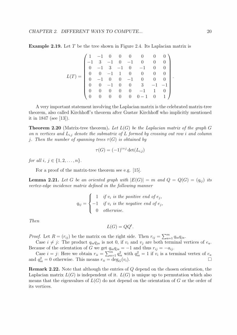
Example 2.19. Let T be the tree shown in Figure 2.4. Its Laplacian matrix is
L(T ) =
1 −1 0 0 0 0 0 0−1 3 −1 0 −1 0 0 00 −1 3 −1 0 −1 0 00 0 −1 1 0 0 0 00 −1 0 0 −1 0 0 00 0 −1 0 0 3 −1 −10 0 0 0 0 −1 1 00 0 0 0 0 0− 1 0 1
.
A very important statement involving the Laplacian matrix is the celebrated matrix-treetheorem, also called Kirchhoff’s theorem after Gustav Kirchhoff who implicitly mentionedit in 1847 (see [13]).
Theorem 2.20 (Matrix-tree theorem). Let L(G) be the Laplacian matrix of the graph Gon n vertices and Li,j denote the submatrix of L formed by crossing out row i and columnj. Then the number of spanning trees τ(G) is obtained by
τ(G) = (−1)i+j det(Li,j)
for all i, j ∈ {1, 2, . . . , n}.
For a proof of the matrix-tree theorem see e.g. [15].
Lemma 2.21. Let G be an oriented graph with |E(G)| = m and Q = Q(G) = (qij) itsvertex-edge incidence matrix defined in the following manner
qij =
1 if vi is the positive end of ej,
−1 if vi is the negative end of ej,
0 otherwise.
ThenL(G) = QQt.
Proof. Let R = (rij) be the matrix on the right side. Then rij =∑m
a=1 qiaqja.Case i 6= j: The product qiaqja is not 0, if vi and vj are both terminal vertices of ea.
Because of the orientation of G we get qiaqja = −1 and thus rij = −aij.Case i = j: Here we obtain rii =
∑ma=1 q
2ia with q2
ia = 1 if vi is a terminal vertex of eaand q2
ia = 0 otherwise. This means rii = degG(vi).
Remark 2.22. Note that although the entries of Q depend on the chosen orientation, theLaplacian matrix L(G) is independent of it. L(G) is unique up to permutation which alsomeans that the eigenvalues of L(G) do not depend on the orientation of G or the order ofits vertices.

CHAPTER 2. DIFFERENT WAYS TO COMPUTE... 21
Unlike L(G) its “edge version” K(G) = QtQ depends on the orientation for the signsof its off-diagonal entries. Due to the singular value decomposition of Q, the eigenvaluesnot equal to 0 of K(G) and L(G) are the same.
Denote the eigenvalues of L(G) by λ1 ≥ λ2 ≥ · · · ≥ λn, then, as the sum over theentries of each row and column is 0, λn = 0 and, following from the matrix-tree theorem,λn−1 > 0 if and only if G is connected.
Lemma 2.23. Let T be a tree on n vertices and K(T ) as before. Then
det(K(T )) = n.
Proof. According to Remark 2.22 we obtain
det(K(T )) =n−1∏i=1
λi
with λi, i ∈ {1, 2, . . . , n − 1}, the eigenvalues of L(T ) not equal to 0. Considering thecharacteristic polynomial of L(T ) it is easy to see that the coefficient coeffλ of λ is
coeffλ = (−1)n−1
n−1∏i=1
λi.
On the other hand, it is well known (see e.g. [14]) that
coeffλ = (−1)n−1
n∑i=1
det(Li,i).
Thus we get
det(K(T )) =n∑i=1
det(Li,i) = n
since Li,i = 1 due to the matrix-tree theorem.
A C B
ei eju
Figure 2.5
Definition 2.6. Let T be a tree and ei, ej two edges of T . Furthermore let T ′ =(V (T ), E(T )\{ei, ej}) be the forest with three components A, B and C, where A andB are on opposite sides of ei and ej such that a path in T from any vertex of A to any ver-tex of B contains ei and ej (see Figure 2.5). Then we define n(ei, ej) = |A| |B|. Analogouslywe use n(ei) = nu(ei)nv(ei) for ei = (u, v).
A vertex u of C is called between ei and ej if every path from a vertex of A to a vertexof B passes through u. The number of vertices between ei and ej is denoted by sij.

CHAPTER 2. DIFFERENT WAYS TO COMPUTE... 22
Lemma 2.24. Let T be a tree on n vertices and orient T such that K(T ) is not negative.Let X = (xij) be the adjugate of K(T ). Then
xij =
{n(ei) if i = j
(−1)sijn(ei, ej) otherwise.
Proof. Denote by Ki,j the submatrix of K(T ) obtained by deleting row i and column j,corresponding, respectively, to edge ei and ej and, analogously, by Qpq,i the submatrix ofQ after deleting the rows p and q, corresponding to the vertices vp and vq, and column i,corresponding to edge ei. Then
xij = (−1)i+j detKi,j
= (−1)i+jn−1∑p=1
n∑q=p+1
detQti,pq detQpq,j
= (−1)i+jn−1∑p=1
n∑q=p+1
detQpq,i detQpq,j. (2.5)
The second equality we get by using the Binet-Cauchy formula as Ki,j = Qti, Q ,j. Thus we
have to compute the determinant for any (n− 2)-square submatrix of Q. Remember thatin each column of Q there are just two non-zero elements. If we delete a row p of Q whichmeans removing vertex vp but not any edges from T , there is exactly one permutation π
such thatn∏l=1l 6=p
qlπ(l) 6= 0. This can easily be seen, as choosing qlπ(l) means to assign edge
eπ(l) to its terminal vertex vl. Analogously we obtain for Qpq,i that there exists exactly onepermutation if and only if the edge ei lies on the path between vp and vq. Therefore we get
detQpq,i =
{±1 if ei is between vp and vq,
0 otherwise.
Considering the case i = j we obtain
xii = (−1)2i
n−1∑p=1
n∑q=p+1
detQpq,i detQpq,i
=n−1∑p=1
n∑q=p+1
(detQpq,i)2
= n(ei)
since xii counts the pairs p, q, p < q, such that ei lies on the path between vp and vq, whichmeans that xii is the product of the numbers of vertices on each side of ei.
CHAPTER 2. DIFFERENT WAYS TO COMPUTE... 23
Now we assume i 6= j and, without loss of generality, we can further assume i < j.In order for a product detQpq,i detQpq,j to be non-zero of course both factors must benon-zero, which is only possible if the vertices vp and vq lie on opposite sides of ei as wellas on opposite sides of ej. Thus |xij| ≤ n(ei, ej), and equality is attained only if the signsof all summands are the same. Recall that we are assuming the orientation of the edgeshas been chosen such that K(T ) is entry-wise non-negative, i.e.
kab =n∑c=1
qcaqcb ≥ 0 ∀a, b.
It is obvious that qcaqcb 6= 0 if and only if ea and eb have vc as their common terminalvertex. Since T is a tree, each pair of edges can have at most one common terminal vertex,i.e. at most one summand can be non-zero. Therefore kab = 0 if ea and eb have no commonterminal vertex, and kab = 1 otherwise. In the second case both edges are oriented thesame way according to their common terminal vertex. This implies that all entries of a rowof Q have the same sign. Hence the only difference between the permutations making acontribution to the computation of detQpq,i and detQpq,j is that for the non-zero elementsof column i and column j one has to choose another non-zero element of the same row. Thusthe only factor to influence the sign of detQpq,i detQpq,j are the signs of the permutations.Let the permutations be denoted by πpq,i and πpq,j and their signs sgn(pq, i) and sgn(pq, j).It is easily seen that the signs depend on both the arbitrary ordering of the vertices andof the edges, but their product only depends on how the edges are ordered since K isindependent of the numbering of the vertices. Thus, we may assume that the verticesbetween ei and ej are consecutively numbered, say k + 1, k + 2, . . ., k + s with s = sij,and vk+1 is a terminal vertex of ei and vk+s a terminal vertex of ej. The only differencebetween the two permutations πpq,i and πpq,j is the assignment of the edges lying on thepath between ei and ej to their terminal edges. If ei is deleted, we obtain the assignmentvk+s ↔ ej and vk+l ↔ (vk+l, vk+l+1) for l = 1, . . ., s−1. On the other hand, if ej is deleted,we get the assignment vk+1 ↔ ei and vk+l ↔ (vk+l−1, vk+l) for l = 2, . . ., s. This means,for getting the permutation πpq,i by changing permutation πpq,j, we perform the followingmatrix operations: move column i past j − i− 1 columns and row k + 1 past s− 1 rows.Therefore
sgn(pq, i) = (−1)j−i−1(−1)s−1sgn(pq, j)
and thus every non-zero product in equation (2.5) has the same sign, namely (−1)sij+j−i.Hence, the absolute value of xij is n(ei, ej) and altogether we obtain
xij = (−1)i+j(−1)sij+j−in(ei, ej)
= (−1)sijn(ei, ej).
Now we have all tools needed to prove the following main statement:

CHAPTER 2. DIFFERENT WAYS TO COMPUTE... 24
Theorem 2.25. Let T be a tree on n vertices and λ1 ≥ · · · ≥ λn−1 > λn = 0 the eigenvaluesof the corresponding Laplacian matrix. Then the Wiener index can be computed as
W (T ) = n
n−1∑i=1
1
λi.
Proof. We choose an orientation of T such that K(T ) is not negative. According toLemma 2.24 the trace of the adjugate X of K(T ) is
tr(X) =n−1∑i=1
xii =∑
e∈E(T )
n(ei).
As shown in Theorem 2.1, the last sum is equal to the Wiener index of T . On the otherhand we know that the trace of a matrix can also be computed by using its eigenvalues.For all λi, i = 1, . . . , n− 1, we obtain that n 1
λiis an eigenvalue of X = nK−1(T ). Thus
tr(X) =n−1∑i=1
n1
λi,
which completes the proof.
Example 2.26. Let T again be the tree in Figure 2.4. Then the non-zero eigenvalues ofL(T ) are approximately
λ1 = 4.81361,
λ2 = 3.73205,
λ3 = 2.52932,
λ4 = λ5 = 1,
λ6 = 0.657077,
λ7 = 0.267949
and according to Theorem 2.25 we obtain W (T ) = 8∑7
i=11λi
= 65.
2.2 Recursive formulas
Up to now we have just seen explicit formulas for computing the Wiener index. In somecases it may be easier not to compute the Wiener index of the tree itself but of specialsubtrees and get the Wiener index of the whole tree as a combination of these subtrees,e.g. when the tree T is obtained by connecting several copies of the tree T ′ at a vertex u,always using the same vertex v′ ∈ V (T ′). Thus, in the following some recursive formulaswill be shown.
Maybe the first idea that occurs if one wants to calculate the Wiener index recursivelyis to take a tree, delete a leaf and compute the Wiener index of the remaining subtree.

CHAPTER 2. DIFFERENT WAYS TO COMPUTE... 25
Theorem 2.27. Let T be a tree on n ≥ 2 vertices and v ∈ V (T ) a leaf of T . Furthermorelet (u, v) ∈ E(T ) and T ′ = T − v be the subgraph of T after deleting v. Then
W (T ) = W (T ′) + dT ′(u) + n− 1.
Proof. Let x and y be two vertices of T . If v 6= x and v 6= y, the distance between x andy does not change after deleting v. Therefore the sum of all these distances is the Wienerindex of T ′. If one of the two vertices is v, w.l.o.g. v = x, then dT (x, y) = dT ′(u, y) + 1.Thus the sum of all n−1 pairs {x, y} equals dT ′(u)+n−1, which completes the proof.
Example 2.28. Consider a tree T with n vertices, obtained by taking Sn−1 and connectinga further vertex v to a leaf u of Sn−1. Using Theorem 2.27 we easily compute
W (T ) = W (Sn−1) + dSn−1(u) + n− 1
= (n− 2)2 + (n− 3)2 + 1 + n− 1
= n2 − n− 2.
Since the fact, that T is a tree, was just used for counting the number of vertex pairs{v, y}, it is obvious that Theorem 2.27 can also be generalized for connected graphs. Westate this formula in the next theorem because of completeness.
Theorem 2.29. Let G be a connected graph and v ∈ V (G) a leaf. Besides let (v, u) ∈ E(G)and G′ = G− v be the subgraph of G after deleting v. Then
W (G) = W (G′) + dG′(u) + |V (G′)|.
A generalization of Theorem 2.27, where not only a leaf but an arbitrary vertex can bedeleted, is given in [3]:
Theorem 2.30. Let T be a tree of order n ≥ 2 as shown in Figure 2.2. Then
W (T ) =m∑i=1
[W (Ti) + (n− |V (Ti)|)dTi(ui)− |V (Ti)|2] + n(n− 1).
Proof. To compute dT (x, y) with x ∈ Ti fixed, we have to consider two cases, according towhether y ∈ Ti or not. If y ∈ Ti, we have dT (x, y) = dTi
(x, y) and the sum of all such pairsis equal to W (Ti).
In case y ∈ Tj, i 6= j, we obtain
dT (x, y) = dTi(x, ui) + dT (ui, v) + dT (uj, v) + dTj
(y, uj).
Thus we get
W (T ) =m∑i=1
[W (Ti) +
1
2
∑x∈Ti
∑y∈Tj
j 6=i
(dTi(x, ui) + dT (ui, v) + dT (uj, v) + dTj
(y, uj))
]

CHAPTER 2. DIFFERENT WAYS TO COMPUTE... 26
=m∑i=1
[W (Ti) +
∑x∈Ti
∑y∈Tj
j 6=i
(dTi(x, ui) + dT (ui, v))
]
=m∑i=1
[W (Ti) +
∑x∈Ti
(dTi(x, ui) + dT (ui, v))(n− |V (Ti)|)
]
=m∑i=1
[W (Ti) + (n− |V (Ti)|)(dTi
(ui) + |V (Ti)|)]
=m∑i=1
[W (Ti) + (n− |V (Ti)|)dTi
(ui)− |V (Ti)|2)
]+ n
m∑i=1
|V (Ti)|
=m∑i=1
[W (Ti) + (n− |V (Ti)|)dTi
(ui)− |V (Ti)|2)
]+ n(n− 1).
Example 2.31. Let T be a tree on n vertices, obtained by taking the path Pl+1 andattaching n− l−1 vertices to one of its leaves v. To compute W (T ) we apply Theorem 2.30with vertex v as the separating point and therefore with n− l − 1 single vertices and onepath of length l as the subtrees. Thus we obtain
W (T ) =n−l−1∑i=1
[0 + (n− 1)0− 12]
(l + 1
3
)+ (n− l)
(l
2
)− l2 + n(n− 1)
=
(l + 1
3
)+ (n− l)
(l
2
)− (n− 1− l)− l2 + n(n− 1)
=
(l
3
)+ (n− l − 1)
(l
2
)+ (n− 1)2.
u
Tu
v
Tv
Figure 2.6: The trees Tu and Tv connected by a path of k new vertices.
In [5] the following formula for the Wiener index of a tree which arises from two treesby connecting them by a path can be found:
Theorem 2.32. Let Tu and Tv be two trees with nu = |V (Tu)| and nv = |V (Tv)| andu ∈ V (Tu) and v ∈ V (Tv) two vertices. T arises from Tu and Tv by connecting u and v by

CHAPTER 2. DIFFERENT WAYS TO COMPUTE... 27
a path on k new vertices (see Figure 2.6). Then
W (T ) = W (Tu) +W (Tv) + (nu + k)dTv(v) + (nv + k)dTu(u) + (k + 1)nunv
+1
2(k2 + k)(nu + nv) +
1
6(k3 − k).
Proof. Let x, y be two vertices of T . Then we distinguish the following cases:Case 1: x, y ∈ V (Ti), i = u, v. It is obvious that dT (x, y) = dTi
(x, y).Case 2: x ∈ V (Tu) and y ∈ V (Tv), then dT (x, y) = dTu(x, u) + dT (u, v)︸ ︷︷ ︸
=k+1
+dTv(v, y).
Case 3: x and y are both new vertices. The contribution of all such vertices is theWiener index of a path of length k − 1.
Case 4: x ∈ V (Ti), i = u, v, and y is one of the new vertices. In this case we obtaindT (x, y) = dTi
(x, i) + dT (i, y).Therefore we get
W (T ) =∑
{x,y}⊆V (Tu)
dTu(x, y) +∑
{x,y}⊆V (Tv)
dTv(x, y)
+∑
x∈V (Tu)
∑y∈V (Tv)
(dTu(x, u) + k + 1 + dTv(v, y)) +
(k + 1
3
)
+∑y newvertex
( ∑x∈V (Tu)
(dTu(x, u) + dT (u, y)) +∑
x∈V (Tv)
(dTv(x, v) + dT (v, y))
)
= W (Tu) +W (Tv) + dTu(u)nv + nunv(k + 1) + dTv(v)nu +1
6(k3 − k)
+ kdTu(u) + (nu + nv)k∑i=1
i+ kdTv(v)
= W (Tu) +W (Tv) + (nu + k)dTv(v) + (nv + k)dTu(u) + (k + 1)nunv
+1
2(k2 + k)(nu + nv) +
1
6(k3 − k),
which completes the proof.
Example 2.33. Let T be the tree arising from S14 and S19 by connecting the branchingpoint u of S14 with the branching point v of S19 by a path on 12 new vertices. It is easyto see that dS14(u) = 13 and dS19(v) = 18. Furthermore we know that W (Sl) = (l − 1)2.Thus we obtain
W (T ) = 132 + 182 + (14 + 12)18 + (19 + 12)13 + 13 · 14 · 19
+1
2(122 + 12)(19 + 14) +
1
6(123 − 12) = 7682.
Remark 2.34. Since nowhere in the proof of Theorem 2.32 the fact that Tu and Tv aretrees has been used, it is obvious that the formula remains the same for Tu and Tv arbitrarygraphs.

CHAPTER 2. DIFFERENT WAYS TO COMPUTE... 28
Corollary 2.35. Let Tu and Tv be two trees of orders nu and nv, respectively, and verticesu ∈ V (Tu), v ∈ V (Tv). If T arises from Tu and Tv by connecting u and v by an edge,
W (T ) = W (Tu) +W (Tv) + nudTv(v) + nvdTu(u) + nunv.
Proof. Evidently this formula is exactly the formula of Theorem 2.32 with k = 0.
In the same paper they suggest a different way of connecting two trees: To take a pathof each tree containing no branching points and to identify these vertices in the same orderas they appear within the paths. This leads to the following theorem:
Theorem 2.36. Let T1 and T2 be two trees with n1 = |V (T1)| and n2 = |V (T2)|. Fur-thermore let p1 = (u1, u2, . . . , uk) be a path in T1 and p2 = (v1, v2, . . . , vk) a path in T2,both without branching points. Then the Wiener index of the tree T , which is obtained byidentifying ui and vi, i = 1, . . . , k, can be computed as
W (T ) = W (T1) +W (T2) + (n1 − k)dT2(v1) + (n2 − k)dT1(u1)
+ 2(k − 1)[nuk(p1) + nvk
(p2)− nuk(p1)nvk
(p2)]
− 1
2k(k − 1)(n1 + n2) +
1
6(k − 1)(5k2 − k − 12),
where nuk(p1) is the number of vertices in the connected component of T1 containing uk
after deleting all edges of p1 and nvk(p2) is defined analogously.
Proof. Let T ′1, T ′′1 , T ′2 and T ′′2 be defined as shown in Figure 2.7. Then |V (T ′′1 )| = nuk(p1)−1,
|V (T ′′2 )| = nvk(p2) − 1 and with that, we trivially get |V (T ′1)| = n1 − nuk
(p1) − k + 1,|V (T ′2)| = n2 − nvk
(p2)− k + 1.
T ′1
T ′2
u1 = v1 u2 u3 uk−1
v2 v3 vk+1
T ′′1
T ′′2
uk = vk
Figure 2.7
To calculate the Wiener index of T we once again distinguish between some differenttypes of vertex pairs:
Of course all the distances between vertices of T1 keep being the same, for whichreason the contribution of these vertices is W (T1). Under the same considerations, thecontribution of vertex pairs of T2 is W (T2). As the vertices of p1 and p2 are identified we
CHAPTER 2. DIFFERENT WAYS TO COMPUTE... 29
have to subtract all distances between these vertices once (they are counted once in W (T1)and once in W (T2)), which is
(k+1
3
).
Next we calculate the distances within T2 between vertices of T ′1 and vertices of T2−p2.Clearly each vertex of T ′1 contributes dT2(v1)−
(k2
)where the second term compensates for
the fact that dT2(v1) also includes the distances to the vertices of p2. In the same mannerwe obtain dT1(u1)−
(k2
)for the distance within T1 between a vertex of T ′2 and all vertices
of T1 − p1.Using also v1 as the point of reference we get dT2(v1) −
(k2
)− (k − 1)(nvk
(p2) − 1) asthe distances within T2 between a vertex of T ′′1 and all vertices of T2 − p2. The third termoccurs because for all vertices of T ′′2 the (not needed) path between v1 and vk is countedin dT2(v1). Analogously we obtain dT1(u1) −
(k2
)− (k − 1)(nuk
(p1) − 1) for the distanceswithin T2 between a vertex of T ′′2 and all vertices of T1 − p1.
Combining all cases we get
W (T ) = W (T1) +W (T2)−(k + 1
3
)+ (n1 − nuk
(p1)− k + 1)
(dT2(v1)−
(k
2
))+ (n2 − nvk
(p2)− k + 1)
(dT1(u1)−
(k
2
))+ (nuk
(p1)− 1)
(dT2(v1)−
(k
2
)− (k − 1)(nvk
(p2)− 1)
)+ (nvk
(p2)− 1)
(dT1(u1)−
(k
2
)− (k − 1)(nuk
(p1)− 1)
)= W (T1) +W (T2)− 1
6(k − 1)(k2 + k) + (n1 − k)dT2(v1) + (n2 − k)dT1(u1)
− 1
2k(k − 1)(n1 + n2 − 2k)− 2(k − 1)(nuk
(p1)− 1)(nvk(p2)− 1)
= W (T1) +W (T2) + (n1 − k)dT2(v1) + (n2 − k)dT1(u1)
+ 2(k − 1)[nuk(p1) + nvk
(p2)− nuk(p1)nvk
(p2)]
− 1
2k(k − 1)(n1 + n2 − 2k) +
1
6(k − 1) (−k2 − k + 6k2 − 12)︸ ︷︷ ︸
=5k2−k−12
,
which completes the proof.
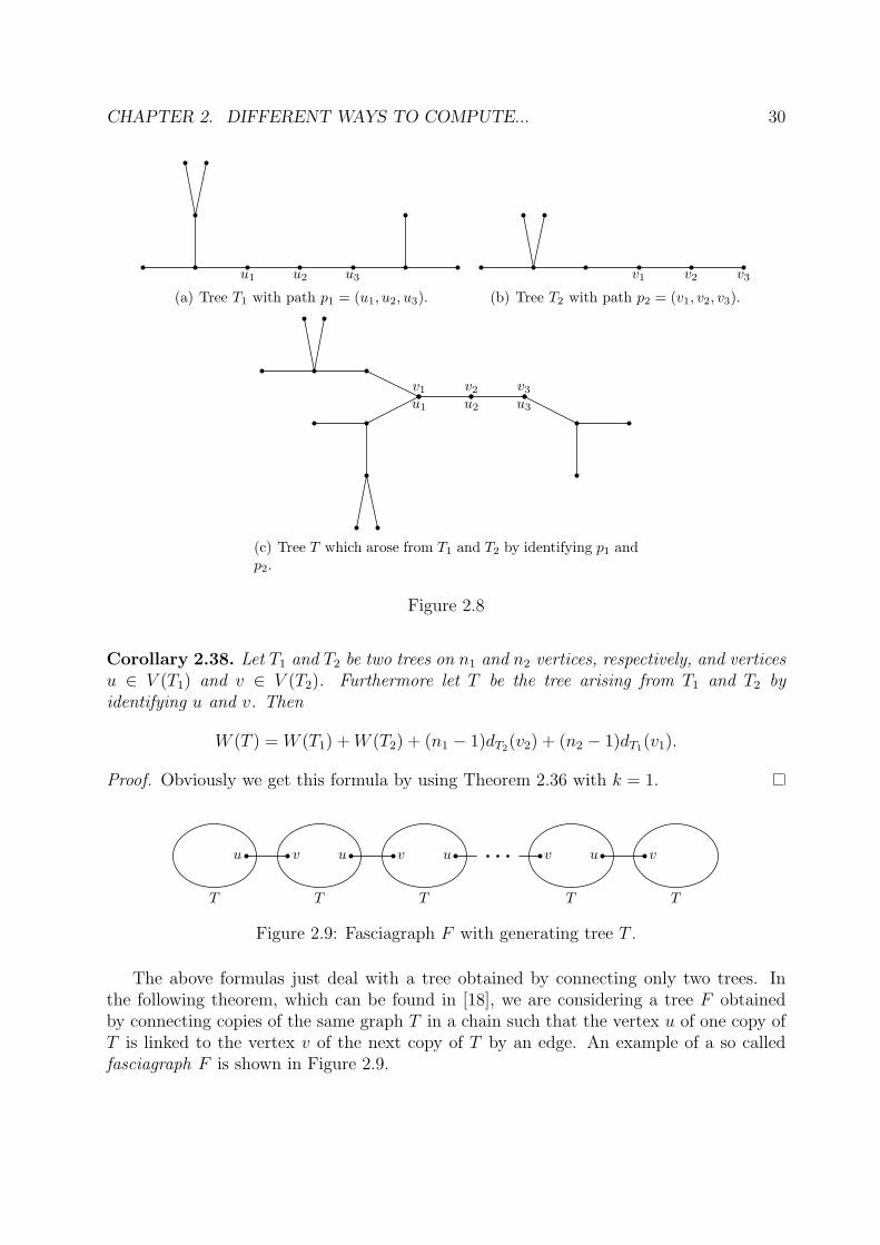
Example 2.37. Let T , T1 and T2 be the trees shown in Figure 2.8. Furthermore letp1 = (u1, u2, u3) and p2 = (v1, v2, v3). Then we have n1 = 11, n2 = 8, k = 3, dT1(u1) = 25,dT2(v1) = 15, nu3(p1) = 4 and nv3(p2) = 1. Besides we easily compute W (T1) = 186 andW (T2) = 71 by using e.g. the Doyle-Graver formula. According Theorem 2.36 we obtain
W (T ) = 186 + 71 + (11− 3)15 + (8− 3)25 + 2 · 2(4 + 1− 4)
− 1
2· 3 · 2(11 + 8) +
1
6· 2(5 · 32 − 3− 12) = 459.
CHAPTER 2. DIFFERENT WAYS TO COMPUTE... 30
u1 u2 u3
(a) Tree T1 with path p1 = (u1, u2, u3).
v1 v2 v3
(b) Tree T2 with path p2 = (v1, v2, v3).
u1 u2 u3
v1 v2 v3
(c) Tree T which arose from T1 and T2 by identifying p1 andp2.
Figure 2.8
Corollary 2.38. Let T1 and T2 be two trees on n1 and n2 vertices, respectively, and verticesu ∈ V (T1) and v ∈ V (T2). Furthermore let T be the tree arising from T1 and T2 byidentifying u and v. Then
W (T ) = W (T1) +W (T2) + (n1 − 1)dT2(v2) + (n2 − 1)dT1(v1).
Proof. Obviously we get this formula by using Theorem 2.36 with k = 1.
u v u v u v u v
T T T T T
Figure 2.9: Fasciagraph F with generating tree T .
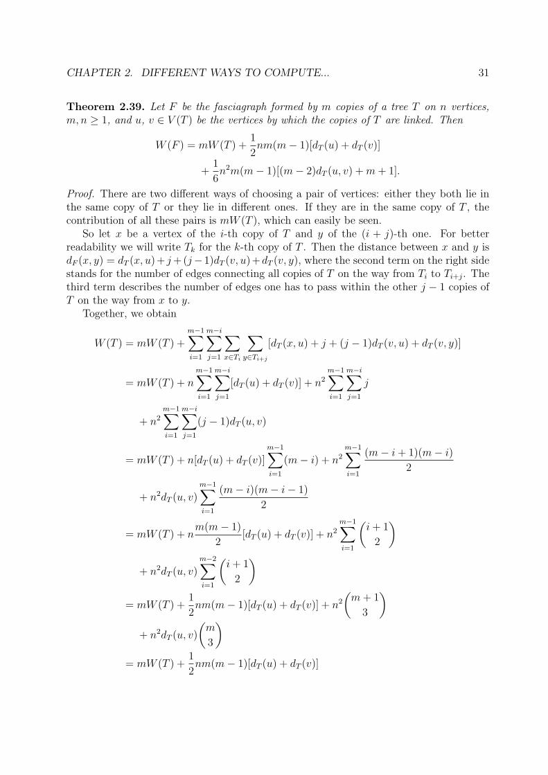
The above formulas just deal with a tree obtained by connecting only two trees. Inthe following theorem, which can be found in [18], we are considering a tree F obtainedby connecting copies of the same graph T in a chain such that the vertex u of one copy ofT is linked to the vertex v of the next copy of T by an edge. An example of a so calledfasciagraph F is shown in Figure 2.9.
CHAPTER 2. DIFFERENT WAYS TO COMPUTE... 31
Theorem 2.39. Let F be the fasciagraph formed by m copies of a tree T on n vertices,m,n ≥ 1, and u, v ∈ V (T ) be the vertices by which the copies of T are linked. Then
W (F ) = mW (T ) +1
2nm(m− 1)[dT (u) + dT (v)]
+1
6n2m(m− 1)[(m− 2)dT (u, v) +m+ 1].
Proof. There are two different ways of choosing a pair of vertices: either they both lie inthe same copy of T or they lie in different ones. If they are in the same copy of T , thecontribution of all these pairs is mW (T ), which can easily be seen.
So let x be a vertex of the i-th copy of T and y of the (i + j)-th one. For betterreadability we will write Tk for the k-th copy of T . Then the distance between x and y isdF (x, y) = dT (x, u) + j+ (j−1)dT (v, u) +dT (v, y), where the second term on the right sidestands for the number of edges connecting all copies of T on the way from Ti to Ti+j. Thethird term describes the number of edges one has to pass within the other j − 1 copies ofT on the way from x to y.
Together, we obtain
W (T ) = mW (T ) +m−1∑i=1
m−i∑j=1
∑x∈Ti
∑y∈Ti+j
[dT (x, u) + j + (j − 1)dT (v, u) + dT (v, y)]
= mW (T ) + nm−1∑i=1
m−i∑j=1
[dT (u) + dT (v)] + n2
m−1∑i=1
m−i∑j=1
j
+ n2
m−1∑i=1
m−i∑j=1
(j − 1)dT (u, v)
= mW (T ) + n[dT (u) + dT (v)]m−1∑i=1
(m− i) + n2
m−1∑i=1
(m− i+ 1)(m− i)2
+ n2dT (u, v)m−1∑i=1
(m− i)(m− i− 1)
2
= mW (T ) + nm(m− 1)
2[dT (u) + dT (v)] + n2
m−1∑i=1
(i+ 1
2
)
+ n2dT (u, v)m−2∑i=1
(i+ 1
2
)= mW (T ) +
1
2nm(m− 1)[dT (u) + dT (v)] + n2
(m+ 1
3
)+ n2dT (u, v)
(m
3
)= mW (T ) +
1
2nm(m− 1)[dT (u) + dT (v)]

CHAPTER 2. DIFFERENT WAYS TO COMPUTE... 32
+1
6n2m(m− 1)[(m− 2)dT (u, v) +m+ 1].
Remark 2.40. Notice that nowhere in the proof of Theorem 2.39 the fact that T is a treewas used. Thus the formula holds also for T an arbitrary connected graph.
Example 2.41. To illustrate Theorem 2.39 we consider the fasciagraph Fn,m obtained byconnecting m copies of the star Sn such that both u and v are the vertex with degreedegSn
(u) = n− 1. Thus we obtain
W (Fn,m) = m(n− 1)2 +1
2nm(m− 1)2(n− 1) +
1
6n2m(m− 1)(m+ 1)
= m[(n− 1)(nm− 1) +1
6n2(m2 − 1)].
2.2.1 The Wiener index of a thorn tree
A completely different concept of reducing the Wiener index of a tree T1 to the Wienerindex of another tree T2 is to add some new leaves to T2:
Definition 2.7. Let T be a tree of order n. Then T ∗ is called thorn tree of T if T ∗ arisesform T by attaching ni new vertices to the vertex vi of T , i = 1, 2, . . ., n.
Remark 2.42. It is obvious that the number of vertices of T ∗ is n∗ = n +∑n
i=1 ni anddegT ∗(vi) = degT (vi) + ni.
Furthermore notice that neither the thorn tree of a given tree nor the tree from whichthe thorn tree has arisen is unique.
Figure 2.10: A tree and its thorn tree.
Example 2.43. An example of a tree T and one of its possible thorn trees T ∗ is given inFigure 2.10, where the dashed edges indicate the new ones of T ∗. As one can see not allvertices of T have to be connected with a new vertex.
The following formula for computing the Wiener index of the thorn tree T ∗ by usingthe Wiener index of the corresponding tree T was given by Gutman in 1998 [10]:

CHAPTER 2. DIFFERENT WAYS TO COMPUTE... 33
Theorem 2.44. Let T be a tree on n vertices and T ∗ its thorn tree. Then
W (T ∗) = W (T ) +∑
1≤i<j≤n
(ni + nj)dT (vi, vj) +∑
1≤i<j≤n
ninjdT (vi, vj)
+
( n∑i=1
ni
)2
+ (n− 1)n∑i=1
ni
=∑
1≤i<j≤n
(ni + 1)(nj + 1)dT (vi, vj) +
( n∑i=1
ni
)2
+ (n− 1)n∑i=1
ni
with ni the number of new vertices connected to vi.
Proof. Let V (T ) = {v1, v2, . . . , vn}. For each pair of vertices x, y ∈ V (T ∗) we distinguishbetween four cases:
Case 1: x ∈ V (T ) and y ∈ V (T ). It is obvious that dT ∗(x, y) = dT (x, y) and thereforethe contribution to the Wiener index of T ∗ of all such vertex pairs is W (T ).
Case 2: x ∈ V (T ), e.g. x = vj, and y ∈ V (T ∗) \ V (T ) with y attached to a vertex vi.Then we obtain for all ni pairs {x, y} that dT ∗(x, y) = dT (x, vi) + 1.
Case 3: x, y ∈ V (T ∗) \ V (T ) with x attached to a vertex vi and y attached to a vertexvj, i 6= j. Then dT ∗(x, y) = dT (vi, vj) + 2, and there are exactly ninj such pairs {x, y}.
Case 4: x, y ∈ V (T ∗) \ V (T ) with both attached to a vertex vi. Then dT ∗(x, y) = 2and the number of such pairs is
(ni
2
).
Altogether we get
W (T ∗) = W (T ) +n∑i=1
n∑j=1
ni(dT (vi, vj) + 1) +∑
1≤i<j≤n
ninj(dT (vi, vj) + 2) +n∑i=1
2
(ni2
)
= W (T ) +∑
1≤i<j≤n
(ni + nj)dT (vi, vj) +n∑i=1
n∑j=1
ni +∑
1≤i<j≤n
ninjdT (vi, vj)
+
( n∑i=1
ni
)2
−n∑i=1
n2i +
n∑i=1
ni(ni − 1)
= W (T ) +∑
1≤i<j≤n
(ni + nj)dT (vi, vj) +∑
1≤i<j≤n
ninjdT (vi, vj)
+
( n∑i=1
ni
)2
+ (n− 1)n∑i=1
ni.
Since W (T ) =∑
1≤i<j≤ndT (vi, vj), we can also write the Wiener index of T ∗ as
W (T ∗) =∑
1≤i<j≤n
(ni + 1)(nj + 1)dT (vi, vj) +
( n∑i=1
ni
)2
+ (n− 1)n∑i=1
ni,
which completes the proof.

CHAPTER 2. DIFFERENT WAYS TO COMPUTE... 34
v1 v2 v3 v4 v5
Figure 2.11
Example 2.45. Let us consider the thorn tree T ∗ shown in Figure 2.11. To use Theo-rem 2.44 for computing the Wiener index of T ∗ we choose the path (v1, v2, v3, v4, v5) to bethe tree T and therefore n1 = 4, n2 = 1, n3 = 3, n4 = 0 and n5 = 2. Thus we obtain
W (T ∗) =5∑i=1
5∑j=i+1
(ni + 1)(nj + 1)|j − i|+( 5∑i=1
ni
)2
+ 45∑i=1
ni
= 186 + 100 + 40 = 326.
Remark 2.46. It is easily seen that in Theorem 2.44 the graph T need not be a tree, butonly a finite, connected and simple graph.
Now let us consider some special cases of Theorem 2.44:
Corollary 2.47. Let T be a tree on n vertices v1, v2, . . . , vn, and T ∗ its thorn tree withni = k, i = 1, 2, . . . , n. Then
W (T ∗) = (k + 1)2W (T ) + nk(nk + n− 1).
Proof. Simple substituting leads to
W (T ∗) = W (T ) +∑
1≤i<j≤n
2kdT (vi, vj) + k2∑
1≤i<j≤n
dT (vi, vj)
+
( n∑i=1
k
)2
+ (n− 1)n∑i=1
k
= (1 + 2k + k2)W (T ) + k2n2 + kn(n− 1)
= (k + 1)2W (T ) + nk(nk + n− 1).
Example 2.48. Let T ∗ arise from the tree T of Figure 2.11 by connecting 3 vertices toeach vertex of T . According to Example 2.45 the Wiener index of T is 326. Therefore weeasily get
W (T ∗) = 4 · 326 + 15 · 3(15 · 3 + 15− 1) = 3959.
To obtain two further corollaries we first have to prove the following lemma:

CHAPTER 2. DIFFERENT WAYS TO COMPUTE... 35
Lemma 2.49. Let T be a tree with vertex set V (T ) = {v1, v2, . . . , vn}. Then∑1≤i<j≤n
(degT (vi) + degT (vj))dT (vi, vj) = 4W (T )− n(n− 1) (2.6)
and ∑1≤i<j≤n
degT (vi) degT (vj)dT (vi, vj) = 4W (T )− (n− 1)(2n− 1). (2.7)
Proof. To prove the two equations we use equation (2.1) in a more generalized form, whichmeans that every pair {vi, vj} is associated with a weight ωij. Since equation (2.1) can berewritten as
W (T ) =∑
e=(va,vb)∈E(T )
∑vi∈V (Ta)
∑vj∈V (Tb)
1
using the notation defined in Theorem 2.6, we obtain by similar considerations
Wω(T ) :=∑
1≤i<j≤n
ωijdT (vi, vj) =∑
e=(va,vb)∈E(T )
∑vi∈V (Ta)
∑vj∈V (Tb)
ωij.
Let ωij = degT (vi) + degT (vj). Then∑1≤i<j≤n
(degT (vi) + degT (vj))dT (vi, vj) =
=∑
e=(va,vb)∈E(T )
( ∑vi∈V (Ta)
∑vj∈V (Tb)
degT (vj) +∑
vi∈V (Ta)
∑vj∈V (Tb)
degT (vj)
)
=∑
e=(va,vb)∈E(T )
(nvb
(e)∑
vi∈V (Ta)
degT (vi) + nva(e)∑
vj∈V (Tb)
degT (vj)
)=
∑e=(va,vb)∈E(T )
(nvb(e)[2(nva(e)− 1) + 1] + nva(e)[2(nvb
(e)− 1) + 1])
=∑
e=(va,vb)∈E(T )
[4nva(e)nvb(e)− (nva(e) + nvb
(e))]
= 4W (T )− n(n− 1).
The third equation holds as∑
v∈V (G) degG(v) = 2|E(G)| for all finite graphs G, and fur-
thermore we use the fact that degT (v) = degTl(v) for all vertices v ∈ V (Tl \ {vl}) and
degT (vl) = degTl(vl)− 1, l = a, b.
Now let ωij = degT (vi) degT (vj). Then∑1≤i<j≤n
(degT (vi) degT (vj))dT (vi, vj) =∑
e=(va,vb)∈E(T )
( ∑vi∈V (Ta)
degT (vi)∑
vj∈V (Tb)
degT (vj)
)

CHAPTER 2. DIFFERENT WAYS TO COMPUTE... 36
=∑
e=(va,vb)∈E(T )
[2(nva(e)− 1) + 1][2(nvb(e)− 1) + 1]
=∑
e=(va,vb)∈E(T )
[4nva(e)nvb(e)− 2(nva(e) + nvb
(e)) + 1]
= 4W (T )− (n− 1)(2n− 1),
which completes the proof.
Corollary 2.50. Let T be a tree of order n and T ∗ its thorn tree with parameters ni =degT (vi), i = 1, 2, . . ., n. Then
W (T ∗) = 9W (T ) + (n− 1)(3n− 5).
Proof. Using Theorem 2.44 and Lemma 2.49 we obtain
W (T ∗) = W (T ) +∑
1≤i<j≤n
(degT (vi) + degT (vj))dT (vi, vj)
+∑
1≤i<j≤n
degT (vi) degT (vj)dT (vi, vj) +
( n∑i=1
degT (vi)
)2
+ (n− 1)n∑i=1
degT (vi)
= W (T ) + 4W (T )− n(n− 1) + 4W (T )− (n− 1)(2n− 1)
+ 4(n− 1)2 + 2(n− 1)2
= 9W (T ) + (n− 1)(3n− 5).
Corollary 2.51. Let T be a tree on n vertices and T ∗ its thorn tree with parametersni = m− degT (vi) ≥ 0, i = 1, 2, . . ., n. Then
W (T ∗) = (m− 1)2W (T ) + [(m− 1)n+ 1]2.
Proof. In the same manner as in Corollary 2.50 we compute
W (T ∗) = W (T ) +∑
1≤i<j≤n
(2m− degT (vi)− degT (vj))dT (vi, vj)
+∑
1≤i<j≤n
(m− degT (vi))(m− degT (vj))dT (vi, vj)
+
( n∑i=1
(m− degT (vi))
)2
+ (n− 1)n∑i=1
(m− degT (vi))
= W (T ) + 2mW (T )− (4W (T )− n(n− 1)) +m2W (T )

CHAPTER 2. DIFFERENT WAYS TO COMPUTE... 37
−m(4W (T )− n(n− 1)) + 4W (T )− (n− 1)(2n− 1)
+ (mn− 2(n− 1))2 + (n− 1)(mn− 2(n− 1))
= (m− 1)2W (T ) + (mn)2 − 2mn(n− 1) + (n− 1)2
= (m− 1)2W (T ) + [(m− 1)n+ 1]2.
Another special case of thorn trees are the so-called caterpillars. In [2] a formula forregular caterpillars is presented.
Definition 2.8. If T is a path, its thorn tree T ∗ is called a caterpillar.We denote a caterpillar by T ∗(a, b) if all vertices which are not leaves have the same
degree a > 1 and b > 0 is the number of non-leaves.
Corollary 2.52. Let T ∗(a, b) be as before. Then
W (T ∗(a, b)) =(a− 1)b
6[(a− 1)(b− 1)(b+ 7) + 6(a+ 1)] + 1.
Proof. Substituting into the formula of Corollary 2.51 we get
W (T ∗(a, b)) = (a− 1)2W (Pb) + [(a− 1)b+ 1]2
= (a− 1)2
(b+ 1
3
)+ (a− 1)2b2 + 2(a− 1)b+ 1
= (a− 1)b
[(a− 1)
(b2 − 1
6+ b
)+ 2
]+ 1
=(a− 1)b
6[(a− 1)(b2 + 6b− 1) + 12] + 1
=(a− 1)b
6[(a− 1)(b− 1)(b+ 7) + 6(a+ 1)] + 1.
2.2.2 A k-subdivision of a tree and its Wiener index
By increasing the length of the segments in a tree we obtain another concept of growingtrees (see [5]):
Definition 2.9. Let T be a tree. T ′ is called k-subdivision of T if T ′ arises from T byreplacing every edge of T by a path of length k + 1.
Notice that the order of T ′ is n′ = k(n − 1) + n and the degree of each new vertex isexactly 2, whereas degT ′(v) = degT (v) for all v ∈ V (T ).

CHAPTER 2. DIFFERENT WAYS TO COMPUTE... 38
Theorem 2.53. Let T be a tree on n vertices and T ′ its k-subdivision. Then
W (T ′) = (k + 1)3W (T ) +
(n′ + 1
3
)− (k + 1)3
(n+ 1
3
)with n′ the order of T ′.
Proof. Applying formula 2.2 to T ′ we get
W (T ′) =
(n′ + 1
3
)−
∑v∈V (T ′)
∑1≤i<j<l≤degT ′ (v)
|V (T ′i )| · |V (T ′j)| · |V (T ′l )|
=
(n′ + 1
3
)−∑
v∈V (T )
∑1≤i<j<l≤degT (v)
(k + 1)3|V (Ti)| · |V (Tj)| · |V (Tl)|
=
(n′ + 1
3
)+ (k + 1)3W (T )− (k + 1)3
(n+ 1
3
).
Example 2.54. Let T be the tree shown in Figure 2.1 and T ′ its 3-subdivision. As wealready know that W (T ) = 250 we can easily compute the Wiener index of T ′ by usingTheorem 2.53. Thus we obtain
W (T ′) = 43 · 250 +
(50
3
)− 43
(14
3
)= 12304.
In [18] Polansky and Bonchev also consider a tree T1 which is obtained from T by1-subdividing only one edge e = (u, v) of T :
Theorem 2.55. Let T be a tree of order n and e = (u, v) ∈ E(T ). Furthermore let T1 bethe tree as described above. Then
W (T1) = W (T ) +1
2[dT (u) + dT (v) + nu(e) + 2nu(e)nv(e) + nv(e)].
Proof. Let the new vertex between u and v be denoted by w. Considering two vertices xand y ∈ V (T1) we distinguish between three cases:
If x, y ∈ V (Tl), l = u, v, we have dT1(x, y) = dT (x, y).If x ∈ V (Tu) and y ∈ V (Tv), we obtain dT1(x, y) = dT (x, y) + 1.If x ∈ V (Tl), l = u, v, and y = w, we get dT1(x, y) = dT (x, l) + 1.
Furthermore it is easy to see that
dT (u) = dTu(u) +∑
x∈V (Tv)
dT (u, v) = dTu(u) + dTv(v) + nv(e)
and analogouslydT (v) = dTu(u) + dTv(v) + nu(e).

CHAPTER 2. DIFFERENT WAYS TO COMPUTE... 39
Altogether we obtain
W (T1) =∑
{x,y}⊆V (Tu)
dT (x, y) +∑
{x,y}⊆V (Tv)
dT (x, y) +∑
x∈V (Tu)
∑y∈V (Tv)
(dT (x, y) + 1)
+∑
x∈V (Tu)
(dT (x, u) + 1) +∑
x∈V (Tv)
(dT (x, v) + 1)
= W (T ) + nu(e)nv(e) + dTu(u) + nu(e) + dTv(v) + nv(e)
= W (T ) + nu(e)nv(e) +1
2[dT (u) + dT (v)− nu(e)− nv(e)] + nu(e) + nv(e)
= W (T ) +1
2[dT (u) + dT (v) + nu(e) + 2nu(e)nv(e) + nv(e)].
Example 2.56. We again choose T to be the tree in Figure 2.1. Furthermore let T1 bethe tree which is obtained by 1-subdividing e = (v4, v5). Since dT (v4) = 27, dT (v5) = 30,nv4(e) = 8 and nv5(e) = 5, we get
W (T1) = 250 +1
2(17 + 30 + 8 + 2 · 8 · 5 + 5) = 325
according to Theorem 2.55.

Chapter 3
Lower and upper bounds
Since calculating the Wiener index of a graph can be computationally expensive, it isof some interest to know the extreme values of the Wiener index, particularly of graphsbelonging to certain classes.
3.1 Bounds for general graphs
Some very basic bounds for the Wiener index are given in [11]. The first inequality men-tioned here shows how the Wiener index of a graph and of its subgraph are related.
Theorem 3.1. Let G be a connected graph and e ∈ E(G). Furthermore let G′ be the graphwith vertex set V (G) and edge set E(G) \ {e}. Then
W (G) < W (G′).
Proof. Let e = (u, v). Then for each vertex pair x, y with e lying on the shortest pathbetween x and y we obviously have dG(x, y) ≤ dG′(x, y). Since dG(u, v) < dG′(u, v), weobtain W (G) < W (G′).
This immediately leads to the following theorem about graphs and their spanning trees:
Theorem 3.2. Let G be a connected graph and T its spanning tree. Then
W (G) ≤ W (T )
with equality if and only if G is a tree.
A lower bound for the Wiener index of an arbitrary graph is given by the next theorem:
Theorem 3.3. Let G be a connected graph. Then
W (G) ≥ n(n− 1)
2.
40

CHAPTER 3. LOWER AND UPPER BOUNDS 41
Proof. The Wiener index of the complete graph Kn on n vertices can be easily computedas
W (Kn) =n−1∑i=1
i =n(n− 1)
2.
According to Theorem 3.1 each subgraph G of Kn with E(G) ⊂ E(Kn) has Wiener indexless than the Wiener index of Kn. Since each graph of order n is a subgraph of the completegraph, the inequality holds.
In [8] closer bounds are given if the number of edges is fixed.
Theorem 3.4. Let G be a connected graph with n vertices and m edges. Then
n(n− 1)−m ≤ W (G) ≤ n3 + 5n− 6
6−m.
Proof. In order to prove the first inequality we consider the distance between two verticesu and v. If u and v are neighbours, we obtain dG(u, v) = 1 and otherwise dG(u, v) ≥ 2.Since |E(G)| = m, there are exactly m unordered vertex pairs with distance 1 and
(n2
)−m
unordered vertex pairs with distance greater than 1. Thus we obtain
W (G) =∑
{u,v}⊆V (G)
dG(u, v) ≥ m+ 2
[(n
2
)−m
]= n(n− 1)−m.
The second inequality is shown by induction on n and n− 1 ≤ m ≤(n2
). For n = 2 the
inequality holds since K2 is the only connected graph and W (K2) = 1 ≤ 8+10−66− 1 = 1.
Now let us assume that the second inequality holds for all connected graphs of order n.Let T be a tree on n + 1 vertices and v a leaf of T . Furthermore let T ′ be the subtree ofT induced by V (T ) \ {v}. Then the inequality holds for T ′ and we obtain
W (T ) = W (T ′) + dT (v) ≤ n3 + 5n− 6
6− (n− 1) +
n∑i=1
i
=(n+ 1)3 + 5(n+ 1)− 6
6− n.
Let us assume that the inequality holds for all connected graphs with n vertices andm ≥ n−1 edges. We consider the connected graph G with n vertices and m+1 edges. SinceG is no tree, it contains an edge e such that G′ with vertex set V (G) and edge set E(G)\{e}is a connected subgraph of G. According to Theorem 3.1 we obtain W (G) ≤ W (G′) − 1.As the assumption holds for G′ we have
W (G) ≤ W (G′)− 1 ≤ n3 + 5n− 6
6−m− 1,
which completes the proof.
CHAPTER 3. LOWER AND UPPER BOUNDS 42
Corollary 3.5. Among all connected graphs of order n the path Pn maximizes the Wienerindex.
Proof. Let G be a connected graph with n vertices and m edges. Since G is connected, wehave n− 1 ≤ m. Due to Theorem 3.4 we have
W (G) ≤ n3 + 5n− 6
6−m ≤ n3 + 5n− 6
6− (n− 1)
=n3 − n
6=
(n+ 1
3
)= W (Pn).
3.2 Bounds for trees
Because of Corollary 3.5 we already have an upper bound for the Wiener index of trees.By Corollary 3.6 we also obtain a lower bound.
Corollary 3.6. Among all trees of order n the star Sn minimizes the Wiener index.
Proof. Since the number of edges in a tree of order n is m = n−1, we obtain by Theorem 3.4
(n− 1)2 ≤ W (T ).
Thus, as W (Sn) = (n− 1)2, the star Sn has the minimal Wiener index among all trees oforder n.
Another question that immediately arises is: Which extremal values of the Wienerindex can be obtained if the order of the tree and its maximum degree or even its entiredegree sequence is given? In the following two subsections we will take a closer look atthese problems.
3.2.1 Trees with given maximum degree
As the maximum degree in Pn is 2, it is obvious that Pn still maximizes the Wiener indexamong all trees of order n and maximum degree at most ∆ ≥ 2. Therefore this subsectionwill be mainly devoted to solve the following problem:
Problem 3.1. What trees minimize the Wiener index among all trees of given order nand maximum degree at most ∆ ≥ 2?
Remark 3.7. If ∆ = 2, the only tree with degree at most 2 and therefore the optimalsolution is the path Pn. Also if n ≤ ∆+1, the problem gets trivial and the optimal solutionis the star Sn+1. Thus Problem 3.1 is only of interest if ∆ ≥ 3 and n > ∆ + 1.

CHAPTER 3. LOWER AND UPPER BOUNDS 43
In order to discuss Problem 3.1 we have to consider a special class of trees described inthe definition below (see [9] ).
Definition 3.2. Let ∆ ≥ 3 and R ∈ {∆ − 1,∆}. Then T (R,∆) is defined as the set ofall trees T which can be embedded in the plane as follows:
Let n = |V (T )|, M0(R,∆) = 1 and Mi(R,∆) = 1 + R
k−1∑j=0
(∆ − 1)j for all i ≥ 1.
Furthermore letMk(R,∆) ≤ n < Mk+1(R,∆)
for some k ≥ 0 andn−Mk(R,∆) = m(∆− 1) + r
with m ≥ 0 and 0 ≤ r < ∆− 1. Then
1. all vertices of T lie on some line R× {i} with 0 ≤ i ≤ k + 1,
2. on line R × {0} there is just one single vertex which has exactly min{n − 1, R}neighbours lying all on line R× {1},
3. on line R×{i}, 1 ≤ i ≤ k−1, every vertex has a unique neighbour on line R×{i−1}and ∆− 1 neighbours on line R× {i+ 1},
4. if v1, . . . , vm+1 are the m + 1 leftmost vertices on line R × {k} such that va lies leftof vb for a < b, then vj has ∆ − 1 neighbours on line R × {k + 1}, 1 ≤ j ≤ m, andvm+1 has r neighbours on line R× {k + 1}.
Figure 3.1: The tree T ∈ T (3, 3) with n = 27.
Example 3.8. An example of an element of T (R,∆) with R = ∆ = 3 is shown inFigure 3.1.
Remark 3.9. For every n ∈ N the set T (R,∆) contains a unique tree T of order n up toisomorphism.
Notice that Mi(R,∆) is the number of vertices being assigned to the lines 0 up to i.

CHAPTER 3. LOWER AND UPPER BOUNDS 44
Definition 3.3. Let T be a tree on n vertices and v ∈ V (T ). A maximal subtree Bcontaining v as a leaf is called a branch of T at v. The weight bw(B) of B is defined as thenumber of edges in B and the branch-weight bw(v) of v is the maximum of the weights ofall branches at v. Then it is easy to see that n =
∑ki=1 bw(Bi) with Bi, i = 1, . . . , k, being
the k branches of T at v.Furthermore the centroid C(T ) of T is the set of vertices in T with minimum branch-
weight.
In [5] the following characterisation of centroids is mentioned:
Theorem 3.10. Let T be a tree of order n and C(T ) its centroid. Then one of the followingholds:
(i) C(T ) = {c} and bw(c) ≤ n−12
,
(ii) C(T ) = {c1, c2} and bw(c1) = bw(c2) = n2.
Proof. Assume that |C(T )| ≥ 3, then there exist pairwise distinct c1, c2, c3 ∈ C(T ). It isobvious that bw(c1) = bw(c2) = bw(c3). Let B1 be the branch of c1 with bw(B1) = bw(c1).Then we distinguish the following cases:
(i) c2, c3 /∈ V (B1),
(ii) c2 /∈ V (B1) and c3 ∈ V (B1) (the case c2 ∈ V (B1) and c3 /∈ V (B1) is the same due tosymmetry),
(iii) c2, c3 ∈ V (B1).
For cases (i) and (ii) we immediately obtain that there exists a branch B2 of c2 withV (B1) ∪ {c1} ⊆ V (B2). Thus we have bw(B2) > bw(B1) = bw(c1) = bw(c2) which is acontradiction.
Now let c2, c3 ∈ V (B1) (case (iii)). If there exists another branch B′1 of c1 with bw(B′1) =bw(B1), we obviously have c2, c3 /∈ V (B′1) and therefore we can use the argumentation ofcases (i) and (ii) to obtain a contradiction. Thus for all branches B′1 6= B1 of c1 we havebw(B′1) < bw(B1). Since c2 and c3 are in the same branch of c1, there exists a vertex vwhich is a neighbour of c1 and lies on the paths from c1 to c2 and from c1 to c3. Thatindicates that v ∈ V (B1) and either v 6= c2 or v 6= c3. W.l.o.g. v 6= c2. Since thereexists a path c1 → v → c2, we obtain that there also exists a branch B2 of c2 withc1, v ∈ V (B2). Let Bv be a branch of v. If c1 ∈ V (Bv), we get V (Bv) ⊂ V (B2) andthus bw(Bv) < bw(B2) ≤ bw(c2) = bw(c1). If c1 /∈ V (Bv), we have V (Bv) ⊂ V (B1)and therefore bw(Bv) < bw(B1) = bw(c1). Hence we obtain bw(v) < bw(c1), which is acontradiction to the assumption that c1 ∈ C(T ).
Therefore |C(T )| ≤ 2. Let C(T ) = {c} and furthermore we assume bw(c) > n−12
. LetB1, B2, . . ., Bk be the branches at c and w.l.o.g. let bw(B1) = bw(c). Furthermore wedenote the vertex of B1 connected with c by u. As E(T ) = n− 1, we get that
k∑i=2
bw(Bi) <n− 1
2.

CHAPTER 3. LOWER AND UPPER BOUNDS 45
Considering the branch Ba of u containing B2, . . ., Bk and c we obtain bw(Ba) <n−1
2+ 1
and thereforebw(Ba) ≤ bw(c).
On the other hand, as the other branches of u are subtrees of B1 without c, their branch-weight is smaller than bw(B1). Altogether we get
bw(u) ≤ bw(c),
which is a contradiction to C(T ) = {c}.In case C(T ) = {c1, c2} it is easy to see that for ci the branch Bi with maximum weight
has to contain cj with i 6= j. Furthermore there are no further vertices on the path betweenc1 and c2 (as otherwise such a vertex would lie in both B1 and B2 and therefore the weightof such a vertex would be less than bw(c1)). Since all edges except (c1, c2), which is countedtwice, are counted exactly once, we get
bw(c1) + bw(c2) = n− 1 + 1 = n
and thus bw(c1) = bw(c2) = n2, which completes the proof.
In order to find a solution to Problem 3.1 we have to prove the following lemma, whichcan be found in [9], first.
Lemma 3.11. Let T ∈ T (R,∆) be of order n with Mk(R,∆) < n < Mk+1(R,∆) forsome k ≥ 1. Furthermore let T0 ∈ T (R,∆) be of order Mk(R,∆) and T arise from T0 byattaching n −Mk(R,∆) new vertices which lie on the line R × {k + 1} to the vertices ofT0 lying on the line R× {k}. Then either W (T ) < W (T ′) or T and T ′ are isomorphic.
Proof. Let T ′ be the tree with minimum Wiener index among all trees which arise fromT0 in the manner described above. Then we show that T ′ and T are isomorphic.
Let v ∈ V (T0) lie on the line R × {i} with 0 ≤ i ≤ k. Furthermore the subtree of T ′
containing v and only vertices lying on a line R×{j} with j > i is denoted by Tv. We callTv full (empty) if all vertices of Tv on line R× {k} have degree ∆ (1).
We choose the following planar embedding of T ′: For each v lying on line R × {i},i ≤ k − 1, beginning with i = k − 1 we consider the subtrees of all neighbours of v online R × {i + 1}. We arrange the subtrees according to the number of their vertices in adecreasing manner, the subtree with most vertices lying leftmost.
Claim: Let the vertex v lie on line R × {i}, i ≤ k − 1. Furthermore we denote theneighbours of v on line R×{i+ 1} by v1, . . ., vl. Then there exists at most one tree amongTv1 , . . ., Tvl
which is neither full nor empty.If the claim holds, with this particular planar embedding of T ′ it is easy to see that T ′
and T are isomorphic.Proof of the claim: In order to prove the claim by contradiction we assume that there
exists a vertex v lying on line R × {i} with maximum i, i ≤ k − 1, such that v has atleast two neighbours v1 and v2 on line R × {i + 1} with Tv1 , Tv2 being neither full nor

CHAPTER 3. LOWER AND UPPER BOUNDS 46
v1 v2
v
v1 v2
v
(a) Case p = (∆− 1)k−i − |V1|.
v1 v2
v
v1 v2
v
(b) Case p = |V2|.
Figure 3.2: How T ′′ arises from T ′.
empty. W.l.o.g. we assume that |V (Tv1)| ≥ |V (Tv2)|, which also means that v1 lies left ofv2 according to the embedding described above. Since the claim holds for all j > i, thereis at most one vertex in V (Ta), a = 1, 2, on line R× {k} of degree 6= 1, ∆.
Furthermore we define
V1 = {x ∈ Tv1 : x lies on line R× {k + 1}}
and V2 analogously. Thus we get
1 ≤ |V1| ≤ |V2| < (∆− 1)k−i.
Let p = min{(∆ − 1)k−i − |V1|, |V2|}, then obviously 1 ≤ p. The idea is to take p verticesof V2 and to rearrange them such that they are in V1 \ V2. Therefore let x1, . . . , xp be theleftmost vertices of V2, and furthermore with q = d p
∆−1e let y1, . . . , yq be the rightmost
vertices in V (Tv1) on line R× {k} and z1, . . . , zq be the leftmost vertices in V (Tv2) on thesame line, all counted from left to right. Then we define the tree T ′′ with vertex set V (T ′)and edge set(
E(T ′) \ {(xj, zd j∆−1e) : 1 ≤ j ≤ p}
)∪ {(xj, yd j+b
∆−1e) : 1 ≤ j ≤ p}
with b = degT ′(y1)− 1 (see Figure 3.2).If x, y ∈ V (T ′) \ {x1, . . . , xp}, the distance between x and y is the same in T ′′ as in
T ′. Moreover the sum of the distances between all vertex pairs x ∈ {x1, . . . , xp} andy ∈ (V (T ′) \ (V1 ∪ V2)) ∪ {x1, . . . , xp} is also the same in T ′′ as in T ′. Thus we get
W (T ′)−W (T ′′) =∑
x∈{x1,...,xp}y∈(V1∪V2)\{x1,...,xp}
(dT ′(x, y)− dT ′′(x, y)).

CHAPTER 3. LOWER AND UPPER BOUNDS 47
Considering the subtree of T ′′ induced by V (Tv1) ∪ {x1, . . . , xp} it is easy to see that itcontains a tree T ∗v2
∼= Tv2 such that {x1, . . . , xp} ⊆ V (T ∗v2). Let V ∗1 = V1 \ V (T ∗v2
), then∑x∈{x1,...,xp}
y∈(V1\V ∗1 )∪V2\{x1,...,xp}
(dT ′(x, y)− dT ′′(x, y)) = 0.
Thus we obtain
W (T ′)−W (T ′′) =∑
x∈{x1,...,xp}y∈V ∗1
(dT ′(x, y)− dT ′′(x, y))
≥∑
x∈{x1,...,xp}y∈V ∗1
(2(k + 1− i)− 2(k − i)) > 0,
which is a contradiction to the assumption concerning the Wiener index of T ′ and thereforethe claim holds.
In Lemma 3.12 we use the following notation: Let v ∈ V (T ) with T a tree. If thecentroid C(T ) 6= {v}, then let Tv be the subtree of T induced by
{u ∈ V (T ) : dT (u, c) = dT (u, v) + dT (v, c) for all c ∈ C(T )}
(compare definition of collinear). If C(T ) = {v}, then Tv = T .
Lemma 3.12. Let T be a tree on n vertices and maximum degree at most ∆, ∆ ≥ 3,such that W (T ) ≤ W (T ′) for all trees T ′ on n vertices and maximum degree at most ∆.Furthermore let v ∈ V (T ). Then Tv ∈ T (∆− 1,∆) if C(T ) 6= {v}, and Tv ∈ T (∆,∆) ifC(T ) = {v}.
Proof. If n ≤ ∆ + 1, the tree with minimum Wiener index is the star Sn, as mentioned inRemark 3.7, and hence the lemma holds in this case.
Thus let n > ∆ + 1. In order to prove the lemma by induction, we define h(Tv) as themaximum distance of v to a leaf of Tv. In case h(Tv) = 0, we have V (Tv) = {v} and thusTv ∈ T (∆,∆). If h(Tv) = 1, Tv is a star with degTv
(v) ≤ ∆−1 and, as a result, the lemmaholds too.
Now let h(Tv) ≥ 2.Claim: Let (x1, x2, . . . , xl) be a path in Tv such that x1 = v ∈ C(T ). Then we get
degT (xj) = ∆ for all 1 ≤ j ≤ l − 2.If the claim holds, we distinguish two different cases:
• Case 1: There exist two leaves w1 and w2 in Tv such that dT (v, w2) ≥ dT (v, w1) + 2.
• Case 2: For all leaves w1 and w2 in Tv their distance to v differs by at most 1.

CHAPTER 3. LOWER AND UPPER BOUNDS 48
Ad case 1: We assume that w1 has minimum distance d1 from v among all leaves ofTv and d2 := dT (w2, v) = h(Tv). As for all x 6= v the subtree Tx of Tv is in T (R,∆) withR ∈ {∆ − 1,∆} by induction, the distance between x and a leaf of Tx differs by at most1. Therefore the only subtree containing w1 and w2 is Tv itself. Let v1 and v2, v1 6= v2,be two neighbours of v in Tv such that vi lies on the path between v and wi, i = 1, 2. Byinduction, Tvi
∈ T (∆− 1,∆) for i = 1, 2. Furthermore let u be the neighbour of v2 whichlies on the path between v2 and w2. Therefore we obtain that in the planar embedding ofTv1 and Tv2 according to Definition 3.2 v1 and v2 lie on line R×{0}, u lies on line R×{1},wi lies on line R × {di − 1} for i = 1, 2 and all other vertices in V (Tv1) and V (Tv2) lie onthe lines R× {j} with 1 ≤ j ≤ d1 and 1 ≤ j ≤ d2 − 1, respectively. W.l.o.g. let w2 be thevertex lying leftmost on line R× {d2 − 1} in Tv2 . Furthermore let V1 be the set of verticeson line R × {d1} in Tv1 , let V2 be the set of vertices on line R × {d2 − 1} in Tv2 and letV3 = V (Tv2) \ V (Tu).
Then we easily obtain
|V (Tu)|+ |V3| = |V (Tv2)| ≤ bw(v) ≤ bw(v2) = |V (T ) \ V (Tv2)|.
Hence if |V (Tv1)| < |V (Tu)|, we get
|V3| < |V (T ) \ V (Tv2)| − |V (Tv1)| = |V (T ) \ (V (Tv2) ] V (Tv1))|.
Now we consider the tree T ′ with vertex set V (T ) and edge set
(E(T ) \ {(v, v1), (v2, u)}) ∪ {(v, u), (v2, v1)}.
Then
W (T )−W (T ′) = (|V (Tu)| − |V (Tv1)|) (|V (T ) \ (V (Tv1) ∪ V (Tv2))| − |V3|) > 0,
which is a contradiction.Therefore |V (Tv1)| ≥ |V (Tu)|. Thus we obtain
d2−3∑i=0
(∆− 1)i < |V (Tu)| ≤ |V (Tv1)| <d1∑i=0
(∆− 1)i,
which implies d1 > d2 − 3. According to the definition of d1 and d2, we get d1 = d2 − 2.Hence Tv1 − V1
∼= Tu − V2.As w2 is the leftmost vertex lying on line R× {d1 + 1} of Tv2 , Tu must be full if there
is any vertex of V2 lying in V3, which would be a contradiction to |V (Tv1)| ≥ |V (Tu)| andTv1 not full. Thus we obtain V2 ⊆ V (Tu), and furthermore |V1| ≥ |V2|. This implies that
|V3| ≤ 1 + (∆− 2)
d1−1∑i=0
(∆− 1)i.
In order to construct a tree T ′ such that W (T ) > W (T ′), analogously to the proof ofLemma 3.11 we define p = min{(∆− 1)d1−|V1|, |V2|} ≥ 1. Let x1, . . . , xp be the p leftmost

CHAPTER 3. LOWER AND UPPER BOUNDS 49
vertices in V2. For q = d p∆−1e let y1, . . . , yq be the rightmost q vertices on line R×{d1− 1}
of Tv1 and z1, . . . , zq be the leftmost q vertices on line R×{d1} of Tv2 , all counted from leftto right. Then we define T ′ to be the tree with vertex set V (T ) and edge set(
E(T ) \ {(xj, zd j∆−1e) : 1 ≤ j ≤ p}
)∪ {(xj, yd j+b
∆−1e) : 1 ≤ j ≤ p}
with b = degT ′(y1) − 1. It is obvious that the sum of the distances between all pairs ofvertices in V (T ) \ {x1, . . . , xp} is the same in T and T ′, and analogously the sum of thedistances between all vertex pairs in {x1, . . . , xp}. Thus
W (T )−W (T ′) =∑
x∈{x1,...,xp}y∈V (T )\{x1,...,xp}
(dT (x, y)− dT ′(x, y)).
If x ∈ {x1, . . . , xp} and y ∈ V (T ) \ (V (Tv1) ∪ V (Tv2)), we get dT (x, y) − dT ′(x, y) = 1. Ifx ∈ {x1, . . . , xp} and y ∈ V3, we get dT (x, y)− dT ′(x, y) = −1.
In case C(T ) = {v}, we get degT (v) = ∆ by using the claim. Thus
|V (T ) \ (V (Tv1) ∪ V (Tv2))| ≥ 1 + (∆− 2)
d1−1∑i=0
(∆− 1)i ≥ |V3|.
In case C(T ) 6= {v}, we also get
|V (T ) \ (V (Tv1) ∪ V (Tv2))| > |V (T ) \ V (Tv)| ≥ |V (Tv)| > |V3|.
Altogether we obtain∑x∈{x1,...,xp}
y∈V (T )\(V (Tv1 )∪V (Tu))
(dT (x, y)− dT ′(x, y)) = p(|V (T ) \ (V (Tv1) ∪ V (Tv2))| − |V3|) ≥ 0,
since V (Tu) ∪ V3 = V (Tv2).Considering the subtree of T ′ induced by the vertex set V (Tv1)∪ {x1, . . . , xp} it is easy
to see that it contains a subtree T ∗u∼= Tu with {x1, . . . , xp} ⊆ V (T ∗u ). Let V ∗1 = V1 \V (T ∗u ),
then obviously V ∗1 6= ∅. Thus we get∑x∈{x1,...,xp}
y∈(V (Tv1 )∪V (Tu))\V ∗1
(dT (x, y)− dT ′(x, y)) = 0
and finally ∑x∈{x1,...,xp}
y∈V ∗1
(dT (x, y)− dT ′(x, y)) ≥ p|V ∗1 |((2d1 + 3)− 2d1) > 0.

CHAPTER 3. LOWER AND UPPER BOUNDS 50
Therefore we getW (T )−W (T ′) > 0,
which is a contradiction to the choice of T .Ad case 2: Let Mk(R,∆) ≤ |V (Tv)| < Mk+1(R,∆) for some k ≥ 1. Since in this case
the distance from two leaves of Tv to v differs by at most 1 and the claim implies that allvertices of T except the leaves and their neighbours have degree ∆, T arises from a treeT0 ∈ T (R,∆) of order Mk(R,∆) by attaching n−Mk(R,∆) new vertices which lie on lineR× {k + 1} to the vertices of T0 lying on line R× {k}. Using Lemma 3.11 we obtain thedesired result.
Proof of the claim: Since xi ∈ V (Tv), 2 ≤ i ≤ l, we obtain from the definition of Tv thatxi /∈ C(T ). To prove the claim by contradiction, let degT (xj) < ∆ for some 1 ≤ j ≤ l − 2.Furthermore we define Vj+2 = V (Txj+2
), Vj+1 = V (Txj+1) \ Vj+2 and Vj = V (T ) \ (Vj+1 ∪
Vj+2). Because of the definition of the centroid and Tv, it is easy to see that |Vj| > |Vj+1|.Let T ′′ be the tree with vertex set V (T ) and edge set (E(T )\{(xj+1, xj+2)})∪{(xj, xj+2)}.Then we obtain
W (T )−W (T ′′) = |Vj+2| (|Vj| − |Vj+1|) > 0,
which is a contradiction to the definition of T .
Now we can give the solution to Problem 3.1:
Theorem 3.13. Let T be a tree of order n and maximum degree at most ∆ with ∆ ≥ 3.Then W (T ) ≤ W (T ′) for all trees T ′ of order n and maximum degree at most ∆ if andonly if T ∈ T (∆,∆).
Proof. If C(T ) = {c}, it immediately follows from Lemma 3.12 that T ∈ T (∆,∆).If C(T ) = {c1, c2}, we know from Theorem 3.10 that |V (Tc1)| = |V (Tc2)| = n
2. Further-
more by Lemma 3.12 we obtain Tc1 , Tc2 ∈ T (∆ − 1,∆). Therefore Tc1 and Tc2 must beisomorphic. Because of Lemma 3.11 we get that |V (Tc1)| = |V (Tc2)| = Mk(∆ − 1,∆) forsome k ≥ 0, which implies that T ∈ T (∆,∆).
Since the number of possible trees is finite, there has to be an optimal tree and, as wehave already shown, it has to be in T (∆,∆). Thus if T ∈ T (∆,∆), it is the optimal tree,which completes the proof.
The solution to Problem 3.1 leads to another question:
Problem 3.4. Which trees maximize the Wiener index among all trees of given order n(with n ≡ 2 mod (∆− 1)) whose vertices are either leaves or of degree ∆?
A solution to this problem was also given in [9], but since it is just a special case ofProblem 3.7, we will deal with it later on.

CHAPTER 3. LOWER AND UPPER BOUNDS 51
3.2.2 Trees with given degree sequence
Minimizing the Wiener index
On the following pages we consider the problem described below (see [21]).
Problem 3.5. Given an integer sequence (d1, . . . , dn) with
d1 ≥ d2 ≥ · · · ≥ dk ≥ 2 > 1 = dk+1 = · · · = dn
andn∑i=1
di = 2(n− 1),
we want to find a tree with degree sequence (d1, . . . , dn) which minimizes the Wiener indexamong all trees of the same degree sequence.
Definition 3.6. Let (d1, . . . , dn) be the degree sequence of the tree T with
d1 ≥ d2 ≥ · · · ≥ dk ≥ 2 > 1 = dk+1 = · · · = dn.
Then T is called greedy tree if it can be embedded in the plane as follows:
1. take the vertex v with degree d1 as root,
2. each vertex u lies on some line i where i is the distance between the root v and u,
3. each line is filled up with vertices in decreasing degree order from left to right.
v
Figure 3.3: A greedy tree.
Example 3.14. Let (4, 4, 4, 3, 3, 3, 2, 2, 2, 1, 1, 1, 1, 1, 1, 1, 1, 1, 1, 1) be the given degree se-quence. Then its corresponding greedy tree using the plane embedding of Definition 3.6 isshown in Figure 3.3.
An equivalent definition of a greedy tree is given in the lemma below.
Lemma 3.15. A rooted tree T with a given degree sequence is a greedy tree if the followingholds:

CHAPTER 3. LOWER AND UPPER BOUNDS 52
1. Its root v has the largest degree.
2. For all leaves of T their distance to v differs by at most 1.
3. For any two vertices u1 and u2 with distance to the root dT (v, u1) > dT (v, u2) followsthat degT (u1) ≤ degT (u2).
4. Let u1, u2 be two vertices with dT (v, u1) = dT (v, u2) and degT (u1) > degT (u2). Fur-thermore let w1 and w2 be two more vertices with dT (v, wi) = dT (v, ui) + dT (ui, wi),i = 1, 2, and dT (v, w1) = dT (v, w2). Then we have degT (w1) ≥ degT (w2).
5. Let u1, u2 be two vertices with dT (v, u1) = dT (v, u2) and degT (u1) > degT (u2). Be-sides let u′1, u′2 be two more vertices with dT (v, u′i) = dT (v, ui) and N(u′i)∩N(ui) 6= ∅,i = 1, 2; here N(a) denotes the set of neighbours of the vertex a. Then we havedegT (u′1) ≥ degT (u′2).
For all vertices u′′1, u′′2 with dT (v, u′′1) = dT (v, u′′2) and dT (v, u′′i ) = dT (v, u′i)+dT (u′i, u′′i ),
i = 1, 2, we also have degT (u′′1) ≥ degT (u′′2).
Before being able to show that the greedy tree is the optimal solution to Problem 3.5we have to give some characteristics of paths and the longest path in particular of theoptimal tree. In order to do so, we use the following notation:
Let T be an optimal tree according to Problem 3.5 and P be a path of T . If P is ofodd length, let z be the vertex of P that separates P into two sub-paths of equal length m.Then we denote the vertices of P on the right side of z by x1, x2, . . . , xm and on the leftside by y1, y2, . . . , ym, in both cases the counting starts at z. In case P is of even length,an edge e takes the place of z and the vertices of P are labelled analogously.
Let Xi, Yi and Z be the connected components containing xi, yi and z, respectively,after deleting all edges of P . Besides let X>k and Y>k denote the subtrees induced bythe vertex sets V (Xk+1) ∪ V (Xk+2) ∪ . . . ∪ V (Xm) and V (Yk+1) ∪ V (Yk+2) ∪ . . . ∪ V (Ym),respectively.
W.l.o.g. we assume that |V (X1)| ≥ |V (Y1)|.
Lemma 3.16. Let T be a tree with minimum Wiener index among all trees of the samedegree sequence. Furthermore let P be a path of T with |V (Xi)| ≥ |V (Yi)| for i = 1, 2, . . . , kand k = 1, . . . ,m. Then we can assume
|V (X>k)| ≥ |V (Y>k)|.
Proof. If k = m, we have V (X>k) = V (Y>k) = ∅ and the lemma holds. So, let k < m. Toshow the lemma by contradiction, let us assume that |V (X>k)| < |V (Y>k)|. Let T ′ be thetree which arises from T by switching X>k and Y>k. It is obvious that T ′ and T have thesame degree sequence. Furthermore we show that W (T ′) ≤ W (T ). In order to do so wehave to distinguish between two cases according to whether P contains a vertex z or not.
Considering the case that there is no such vertex z, the distance between two verticesin T ′ is as follows:

CHAPTER 3. LOWER AND UPPER BOUNDS 53
• If x, y ∈ V (X>k) ∪ V (Y>k), we get dT ′(x, y) = dT (x, y).
• If x, y ∈ V (T ) \ (V (X>k) ∪ V (Y>k)), we have dT ′(x, y) = dT (x, y).
• If x ∈ V (A>k) and y ∈ V (Ai), we get dT ′(x, y) = dT (x, y) + 2i − 1 for i = 1, . . . , kand A = X, Y .
• If x ∈ V (X>k) and y ∈ V (Yi) or x ∈ V (Y>k) and y ∈ V (Xi), i = 1, . . . , k, we obtaindT ′(x, y) = dT (x, y)− (2i− 1).
Thus
W (T ′)−W (T ) =k∑i=1
(2i− 1)|V (Xi)||V (X>k)|+k∑i=1
(2i− 1)|V (Yi)||V (Y>k)|
−k∑i=1
(2i− 1)|V (Xi)||V (Y>k)| −k∑i=1
(2i− 1)|V (Yi)||V (X>k)|
=k∑i=1
(2i− 1)(|V (Xi)| − |V (Yi)|︸ ︷︷ ︸≥0
)(|V (X>k)| − |V (Y>k)|︸ ︷︷ ︸<0
) ≤ 0.
In case there is a vertex z ∈ V (P ), the distance between two vertices in T ′ can becalculated as follows:
• If x, y ∈ V (X>k) ∪ V (Y>k), we get dT ′(x, y) = dT (x, y).
• If x, y ∈ V (T ) \ (V (X>k) ∪ V (Y>k)), we have dT ′(x, y) = dT (x, y).
• If x ∈ V (Z) and y ∈ V (A>k) with A = X, Y , we obtain dT ′(x, y) = dT (x, y).
• If x ∈ V (A>k) and y ∈ V (Ai), we get dT ′(x, y) = dT (x, y) + 2i for i = 1, . . . , k andA = X, Y .
• If x ∈ V (X>k) and y ∈ V (Yi) or x ∈ V (Y>k) and y ∈ V (Xi), i = 1, . . . , k, we obtaindT ′(x, y) = dT (x, y)− 2i.
Analogously we get
W (T ′)−W (T ) =k∑i=1
2i(|V (Xi)| − |V (Yi)|)(|V (X>k)| − |V (Y>k)|) ≤ 0,
which completes the proof.
Lemma 3.17. Let T be a tree with minimum Wiener index among all trees of the same de-gree sequence. Furthermore let P be a path of T with |V (Xi)| ≥ |V (Yi)| for i = 1, 2, . . . , k−1and |V (X>k)| ≥ |V (Y>k)|, k = 1, . . . ,m− 1. Then we can assume
|V (Xk)| ≥ |V (Yk)|.

CHAPTER 3. LOWER AND UPPER BOUNDS 54
Proof. Let us assume that |V (Xk)| < |V (Yk)|. Furthermore let T ′ be the tree obtainedfrom T by switching Xk and Yk. We show that W (T ′) ≤ W (T ) by the same case distinctionas in the proof of Lemma 3.16. Thus we obtain for z /∈ V (P )
W (T ′)−W (T ) =k−1∑i=1
(2i− 1)(|V (Xi)| − |V (Yi)|)(|V (Xk)| − |V (Yk)|)
+ (2k − 1)(|V (X>k)| − |V (Y>k)|)(|V (Xk)| − |V (Yk)|) ≤ 0,
and for z ∈ V (P )
W (T ′)−W (T ) =k−1∑i=1
2i(|V (Xi)| − |V (Yi)|)(|V (Xk)| − |V (Yk)|)
+ 2k(|V (X>k)| − |V (Y>k)|)(|V (Xk)| − |V (Yk)|) ≤ 0.
Lemma 3.18. Let T be a tree with minimum Wiener index among all trees of the same de-gree sequence. Furthermore let P be a path of T with |V (Xi)| ≥ |V (Yi)| for i = 1, 2, . . . , k−1and V (X>k−1)| ≥ |V (Y>k−1)|, k = 1, . . . ,m. Then we can assume
degT (xk) ≥ degT (yk).
Proof. For contradiction let us assume that a = degT (xk) < degT (yk) = a+b with a, b ≥ 1.Thus deleting yk leads to a + b connected components. We choose C1, . . . , Cb to be suchcomponents that no vertex of V (P ) is one of their elements. Furthermore let u1, . . . , ub bethe neighbours of yk lying in C1, . . . , Cb and let B be the set of all vertices in C1, . . . , Cb.Then we define T ′ to be the tree with vertex set V (T ) and edge set
(E(T ) \ {(yk, ui) : i = 1, . . . , b}) ∪ {(xk, ui) : i = 1, . . . , b}.
Thus T ′ and T have the same degree sequence and, similar to the previous proofs, we getfor z /∈ V (P )
W (T ′)−W (T ) =k−1∑i=1
(2i− 1) |B|︸︷︷︸>0
(|V (Yi)| − |V (Xi)|)︸ ︷︷ ︸≤0
+ (2k − 1) |B|︸︷︷︸>0
(|V (Y>k−1)| − |B| − |V (X>k−1)|)︸ ︷︷ ︸≤0
≤ 0,
and for z ∈ V (P )
W (T ′)−W (T ) =k−1∑i=1
2i|B|(|V (Yi)| − |V (Xi)|)
+ 2k|B|(|V (Y>k−1)| − |B| − |V (X>k−1)|) ≤ 0.
Therefore in both cases the Wiener index of T ′ is at most as great as the Wiener index ofT , although degT ′(xk) ≥ degT ′(yk).

CHAPTER 3. LOWER AND UPPER BOUNDS 55
Remark 3.19. If at least one inequality in the conditions of Lemma 3.16, Lemma 3.17 orLemma 3.18 is strict, the assumptions in the conclusions become forced.
Up to now we have considered arbitrary paths in a tree T which is an optimal solutionto the Problem 3.5. Now, let P ∗ be a maximal path of T . If P ∗ has odd length 2m− 1, welabel its vertices as vl1 , . . . , v1, u1, . . . , ul2 in this order with l1 + l2 = 2m. If P ∗ has evenlength 2m, we label them as vl1 , . . . , v1, u1, . . . , ul2+1 in this order with l1 + l2 + 1 = 2m+ 1.
Analogously we label the connected components of T which are obtained by deletingall edges of P as Ui and Vi, respectively. We choose the labelling such that U1 is thecomponent with most vertices.
Lemma 3.20. Let T be a tree with minimum Wiener index among all trees of the samedegree sequence. Furthermore let P ∗ be a maximal path of T . Then we can assume that
|V (U1)| ≥ |V (V1)| ≥ |V (U2)| ≥ |V (V2)| ≥ · · · ≥ |V (Um)| = |V (Vm)| = 1
for P ∗ having odd length 2m− 1 and
|V (U1)| ≥ |V (V1)| ≥ |V (U2)| ≥ |V (V2)| ≥ · · · ≥ |V (Vm)| = |V (Um+1)| = 1
for P ∗ having even length 2m. In both cases we have l1 = l2 = m.
Proof. We show the lemma by induction. So, let P ∗ be of odd length. Since U1 is thecomponent with most vertices, we have |V (U1)| ≥ |V (V1)| and |V (U1)| ≥ |V (U2)|. If|V (U2)| > |V (V1)|, we just need to switch U2 and V1 to get
|V (U1)| ≥ |V (V1)| ≥ |V (U2)|.
Now suppose that we have
|V (U1)| ≥ |V (V1)| ≥ |V (U2)| ≥ |V (V2)| ≥ · · · ≥ |V (Vk−1)| ≥ |V (Uk)|
for some k ≤ min{l1, l2}. To show that we can assume |V (Uk)| ≥ |V (Vk)| we suppose that|V (Uk)| < |V (Vk)| must hold. According to Lemma 3.16 applied to the labelling xi = uiand yi = vi, i = 1, . . . , k − 1, we have |V (U>k−1)| ≥ |V (V>k−1)|. Together we obtain
|V (U>k)| = |V (U>k−1)| − |V (Uk)| > |V (V>k−1)| − |V (Vk)| = |V (V>k)|.
Thus we can apply Lemma 3.17 and we get |V (Uk)| ≥ |V (Vk)|, which is a contradiction.Therefore we have
|V (U1)| ≥ |V (V1)| ≥ |V (U2)| ≥ |V (V2)| ≥ · · · ≥ |V (Uk)| ≥ |V (Vk)|.
Analogously we show that |V (Vk)| ≥ |V (Uk+1)| for k < min{l1, l2} by assuming that|V (Vk)| < |V (Uk+1)|. Using the labelling z = u1, xi = vi and yi = ui+1, i = 1, . . . , k − 1,we get
|V (V>k−1)| = |V (X>k−1)| ≥ |V (Y>k−1)| = |V (U>k)|

CHAPTER 3. LOWER AND UPPER BOUNDS 56
by Lemma 3.16. If |V (Yk)| = |V (Uk+1)| > |V (Vk)| = |V (Xk)| holds, we get
|V (U>k+1)| = |V (U>k)| − |V (Uk+1)| > |V (V>k−1)| − |V (Vk)| = |V (V>k)|.
Applying Lemma 3.17 shows that |V (Vk)| ≥ |V (Uk+1)| must hold, which is a contradiction.Thus we have
|V (U1)| ≥ |V (V1)| ≥ |V (U2)| ≥ |V (V2)| ≥ · · · ≥ |V (Vk)| ≥ |V (Uk+1)|.
Altogether we have
|V (U1)| ≥ |V (V1) ≥ · · · ≥ |V (Uk)| ≥ |V (Vk)|
with k = min{l1, l2}. If k = l2, we obtain that |V (U>k)| = 0 since P ∗ is maximal. Accordingto Lemma 3.16 we have |V (V>k)| = 0 and thus l1 = l2 = m. If k = l1 < l2 we analogouslyget that |V (V>k)| = 0. Using the labelling z = u1, xi = vi and yi = ui+1, i = 1, . . . , k,we obtain |V (U>k+1| = 0 by Lemma 3.16. Therefore we have l1 ≤ l2 ≤ l1 + 1. In casel2 = l1 + 1, we get l1 + l2 = 2l1 + 1, which is a contradiction to the assumption that P ∗ hasodd length. Thus
l1 = l2 = m
and, since P ∗ is maximal,|V (Um)| = |V (Vm)| = 1.
If P ∗ has even length, the proof is analogous.
Lemma 3.21. Let T be a tree with minimum Wiener index among all trees of the samedegree sequence. Furthermore let P ∗ be a maximal path of T with labelling such thatLemma 3.20 holds. Then we have
degT (u1) ≥ degT (v1) ≥ degT (u2) ≥ degT (v2) ≥ · · · ≥ degT (um) = degT (vm) = 1
for P ∗ having odd length 2m− 1 and
degT (u1) ≥ degT (v1) ≥ degT (u2) ≥ degT (v2) ≥ · · · ≥ degT (vm) = degT (um+1) = 1
for P ∗ having even length 2m.
Proof. In case P ∗ has odd length, we have according to Lemma 3.20
|V (U1)| ≥ |V (V1)| ≥ |V (U2)| ≥ |V (V2)| ≥ · · · ≥ |V (Um)| = |V (Vm)| = 1.
Thus we obtain
|V (U>i−1)| =m∑k=i
|V (Uk)| ≥m∑k=i
|V (Vk)| = |V (V>i−1)|
CHAPTER 3. LOWER AND UPPER BOUNDS 57
for i = 1, . . . ,m. Applying Lemma 3.18 to P ∗ in the setting that xi = ui and yi = vi fori = 1, . . . ,m leads to degT (xi) ≥ degT (yi), which means
degT (ui) ≥ degT (vi) i = 1, . . . ,m.
On the other hand we have
|V (V>i−1)| =m∑k=i
|V (Vk)| ≥m∑
k=i+1
|V (Uk)| = |V (U>i)|
for i = 1, . . . ,m. Using the assignment z = u1, xi = vi and yi = ui+1 with i = 1, . . . ,m−1,we get degT (xi) ≥ degT (yi) by applying Lemma 3.18, which means
degT (vi) ≥ degT (ui+1) i = 1, . . . ,m− 1.
As |V (Um)| = |V (Vm)| = 1, we further have
degT (um) = degT (vm) = 1.
Altogether we obtain
degT (u1) ≥ degT (v1) ≥ degT (u2) ≥ degT (v2) ≥ · · · ≥ degT (um) = degT (vm) = 1.
It is easy to see that the proof of the second case is analogous.
Finally we once again need the concept of the centroid of a tree and one further char-acteristic of centroids which can be found in [24]:
Theorem 3.22. Let T be a tree and C(T ) its centroid. Then we have dT (c) ≤ dT (v) forall c ∈ C(T ) and v ∈ V (T ).
Proof. Let v ∈ V (T ) with v 6= c and P be the path between v and c. Furthermore letB1, . . . , Bk be the branches of c such that v ∈ V (B1). Let l ≥ 1 be the length of P and letB′i be the subtree of T induced by V (Bi) \ {c}. Then we have the following three cases:
• If x ∈ V (k⋃i=2
B′i), we get dT (v, x) = dT (c, x) + l.
• For all x ∈ V (P ) the sums over their distances to v and c, respectively, cancel eachother out.
• If x ∈ V (B′1) \ V (P ), we have dT (c, x) ≤ dT (v, x) + l.
If |C(T )| = 1, we have n−12≥ bw(B1) = |V (B′1)| according to Theorem 3.10 and thus
we get n+12≤ |V (
k⋃i=2
Bi)| = |V (k⋃i=2
B′i)|+ 1. Therefore we have
|V (B′1) \ V (P )| ≤ n− 1
2− l ≤ n− 3
2<n− 1
2≤ |V (
k⋃i=2
B′i)|

CHAPTER 3. LOWER AND UPPER BOUNDS 58
and we obtain
dT (v)− dT (c) ≥∑
x∈V (kS
i=2B′i)
l −∑
x∈V (B′1)\V (P )
l > 0.
If |C(T )| = 2 and v ∈ C(T ), we have n2
= bw(B1) = |V (B′1)| according to Theorem 3.10
and therefore we obtain n2
= |V (k⋃i=2
Bi)| = |V (k⋃i=2
B′i)|+ 1. Furthermore we have l = 1 and
thusdT (v) = dT (c).
If |C(T )| = 2, v /∈ C(T ) and C(T ) ∩ V (B1) 6= ∅, we again have n2
= bw(B1) = |V (B′1)|
according to Theorem 3.10 and therefore n2
= |V (k⋃i=2
Bi)| = |V (k⋃i=2
B′i)| + 1. Furthermore
in this case we have l ≥ 2 and thus
dT (v)− dT (c) > 0.
If |C(T )| = 2, v /∈ C(T ) and C(T )∩V (B1) = ∅, we get n2> bw(B1) = |V (B′1)| according
to Theorem 3.10 and n2< |V (
k⋃i=2
Bi)| = |V (k⋃i=2
B′i)|+ 1, as n has to be even. With this and
l ≥ 1 we obtaindT (v)− dT (c) > 0,
which completes the proof.
Lemma 3.23. Let T be a tree. Considering any maximal path P ∗ of T with labelling asin Lemma 3.20, then
dT (u1) ≤ dT (x)
for all x ∈ V (P ∗).
Proof. If u1 ∈ C(T ) everything is done according to Theorem 3.22. Thus let us assumethat u1 /∈ C(T ).
Let c ∈ C(T ) with c /∈ V (P ∗). Then it is obvious that there must be a branch B1 ofc such that V (P ∗) ⊆ V (B1). As |V (B1)| ≤ n
2according to Theorem 3.10 and U1 is the
component with most vertices, there must be a path between u1 and c such that no othervertex of P ∗ lies on it. Thus dT (u1) ≤ dT (x) for all x ∈ V (P ∗).
Now, let C(T ) ⊆ V (P ∗) and c ∈ C(T ). Hence there exists a k such that c = uk orc = vk. We consider the case that c = uk, the other one is similar. As u1 /∈ C(T ), wehave c 6= u1. For the distance between u1 and a vertex x we distinguish the following threecases:
• For x ∈ V (V>0) ∪ V (U1) we obtain dT (u1, x) = dT (uk, x)− (k − 1).
• If x ∈ V (U>k−1), we get dT (u1, x) = dT (uk, x) + (k − 1).

CHAPTER 3. LOWER AND UPPER BOUNDS 59
• If x ∈ V (Ui), 2 ≤ i ≤ k − 1, we have dT (u1, x) = dT (uk, x) + (2i− k − 1).
Thus we obtain for k ≥ 2
dT (u1)− dT (uk) =∑
x∈V (V>0)∪V (U1)
−(k − 1) +∑
x∈V (U>k−1)
(k − 1)
+k−1∑i=2
∑x∈V (Ui)
(2i− k − 1)
= − (k − 1)(|V (V>0)|+ |V (U1)|) + (k − 1)|V (U>k−1)|
+k−1∑i=2
|V (Ui)|(2i− k − 1)
≤ − (k − 1)|U1| − (k − 1)k−2∑i=1
|V (Vi)|
+k−1∑i=2
|V (Ui)|(2i− k − 1)
≤ 0,
where the first inequality holds due to |V (Vi)| ≥ |V (Ui+1)| and the second one holds ask − 3 ≥ 2i − k − 1 for i ≤ k − 1 and hence −(k − 1)|V (Vi)| + (2i − k + 1)|V (Ui+1)| ≤ 0.But this is a contradiction to the fact that u1 /∈ C(T ). Thus, according to Theorem 3.22,we obtain dT (u1) ≤ dT (x) for all x ∈ V (P ∗).
Now we can prove the following theorem given in [21] which settles Problem 3.5:
Theorem 3.24. Let (d1, . . . , dn) be an integer sequence with
d1 ≥ d2 ≥ · · · ≥ dk ≥ 2 > 1 = dk+1 = · · · = dn
andn∑i=1
di = 2(n− 1).
Then the greedy tree with degree sequence (d1, . . . , dn) minimizes the Wiener index amongall trees with same degree sequence.
Proof. Let T be the tree which minimizes the Wiener index among all trees with degreesequence (d1, . . . , dn). To show that T is the greedy tree, we show that T fulfils Lemma 3.15.We distinguish two cases: either |C(T )| = 1 or |C(T )| = 2. If there is only one vertex inthe centroid, we choose it as root v. If there are two vertices in C(T ), we choose one as rootv and the other one as its leftmost neighbour. According to Lemma 3.21 and Lemma 3.23v is the vertex with largest degree in T . Thus 1. of Lemma 3.15 is satisfied.

CHAPTER 3. LOWER AND UPPER BOUNDS 60
Let l1 and l2 be two leaves of T . If v lies on the path between l1 and l2, we obtain|dT (l1, v)− dT (l2, v)| ≤ 1 since u1 = v using the labelling of Lemma 3.20. Otherwise thereis a vertex u lying on the path between l1 and l2 such that li is connected with v via u,i = 1, 2. As the path is of maximal length, we can apply Lemma 3.20 to it and obtainu = u1 through similar considerations as made in Lemma 3.23. Thus we have
|dT (l1, v)− dT (l2, v)| = |dT (l1, u)− dT (l2, u)| ≤ 1
and 2. of Lemma 3.15 is satisfied.Let x and y be two vertices with dT (x, v) < dT (y, v). If v, x and y are collinear, we just
choose a path of maximal length such that v, x, y ∈ V (P ). It follows immediately fromLemma 3.21 that degT (x) ≥ degT (y). If v, x and y are not collinear, there exists a vertexu lying on the path P between x and y such that a is connected with v via u, a = x, y. Weprolong P on both sides to gain a path P ′ of maximal length. Again we get that u = u1
and, by using Lemma 3.20, we obtain that x = ui+1, y = vj or x = vi, y = uj+1 withi = dT (x, v)− dT (u, v) and j = dT (y, v)− dT (u, v). Since i < j, we get degT (x) ≥ degT (y)according to Lemma 3.21. Hence 3. of Lemma 3.15 is satisfied.
Now, let x and y be two non-leaves with dT (x, v) = dT (y, v) and degT (x) > degT (y).Moreover let x′ and y′ be two further vertices with
dT (x′, v) = dT (x′, x) + dT (x, v) = dT (y′, y) + dT (y, v) = dT (y′, v).
Let us consider a path P with maximal length and x, y, x′, y′ ∈ V (P ). Applying Lemma 3.20we obtain that there exists a vertex u ∈ V (P ) such that both x and y are connected withv via u and therefore u = u1. Furthermore, as degT (x) > degT (y), we get x = vi,y = ui+1, x′ = vj and y′ = uj+1 with i = dT (x, u) and j = dT (x′, u). Thus we havedegT (x′) ≥ degT (y′) and 4. of Lemma 3.15 is satisfied.
Again, let x and y be two non-leaves with dT (x, v) = dT (y, v) and degT (x) > degT (y)and let u be the vertex lying on the path between x and y such that both x and yare connected with v via u. Furthermore let x′ and y′ be two vertices with dT (x′, v) =dT (y′, v) = dT (x, v) such that a′ and a have a0 as common neighbour, a = x, y. Moreoverlet x′′ and y′′ be two further vertices with
dT (x′′, v) = dT (x′′, x′) + dT (x′, v) = dT (y′′, y′) + dT (y′, v) = dT (y′′, v).
Since 4. of Lemma 3.15 holds, we have degT (x0) ≥ degT (y0). Therefore considering thepath P of maximal length with u, x0, y0, x
′, y′, x′′, y′′ ∈ V (P ), we again obtain u = u1,x0 = vi, y0 = ui+1, x′ = vi+1, y′ = ui+2, x′′ = vj and y′′ = uj+1 with i = dT (x0, u) and j =dT (x′′, u) by applying Lemma 3.20. According to Lemma 3.21 we get degT (x′) ≥ degT (y′)and degT (x′′) ≥ degT (y′′) and 5. of Lemma 3.15 is satisfied.
Finally, by Lemma 3.15, T is the greedy tree.
Maximizing the Wiener index
Problem 3.7. Given an integer sequence (d1, . . . , dn) with
d1 ≥ d2 ≥ · · · ≥ dk ≥ 2 > 1 = dk+1 = · · · = dn

CHAPTER 3. LOWER AND UPPER BOUNDS 61
andn∑i=1
di = 2(n− 1),
we want to find a tree with degree sequence (d1, . . . , dn) which maximizes the Wiener indexamong all trees of the same degree sequence.
Since it is an open problem whether or not finding an optimal solution is NP-hard, wecan only give some characteristics of the optimal solution. The first of these characteristics,which reduces the set of possible solutions to the set of caterpillars, was published by Shiin 1993 (see [19]).
Lemma 3.25. Let (d1, d2, . . . , dn) be a degree sequence with∑n
i=1 di = 2(n − 1). Fur-thermore let Tmax be the tree with maximal Wiener index over all trees which have thisparticular degree sequence. Then Tmax is a caterpillar.
Proof. We prove this theorem by contradiction. So, let us assume that Tmax is not acaterpillar. Then there exists a path of length l ≥ 4.
T1
x1 x2 x3 xk
T2
xk+1 xlP
T3
y
z1 zs
Figure 3.4
Let P = (x1, x2, . . . , xlP ) be a longest path of Tmax. As Tmax is not a caterpillar, thereexists an xk, 2 < k < lP − 1, such that xk is the endpoint of a path P1 not containing anyother vertex of P and having length lP1 ≥ 2. We denote the vertex connected with xk onP1 by y. Then let N(y) = {xk, z1, . . . , zs}, s ≥ 1, be the neighbours of y. Furthermorelet T1 be the subtree of Tmax after deleting the edges (xk, xk+1) and (xk, y) containingxk. By the same operations we get T2 as the subtree containing xk+1 and T3 as the onecontaining y, as illustrated in Figure 3.4. Without loss of generality we can also assumethat |V (T1)| > |V (T2)|.
Now we are going to construct a tree T ′ 6= Tmax, such that W (T ′) > W (T ). In orderto do so we replace each edge (y, zi) of Tmax by the new edge (xlP , zi), i = 1, . . . , s. Hencewe obtain
degT ′(y) = 1 = degTmax(xlP )

CHAPTER 3. LOWER AND UPPER BOUNDS 62
degT ′(xlP ) = degTmax(y)
degT ′(zi) = degTmax(zi)
with i = 1, . . . , s, and therefore the degree sequence of T ′ and Tmax is the same.Now we consider the distance between two vertices. It is easy to see that the distance
within Tmax and T ′ is the same in the following five cases:
• u, v ∈ V (T1)
• u, v ∈ V (T2)
• u, v ∈ V (T3) \ {y}
• u ∈ V (T1), v ∈ V (T2)
• u ∈ V (T1) ∪ V (T2) and y.
Furthermore, as for the degree, xlP takes the place of y and vice versa, concerning thedistance to a vertex in V (T3) \ {y}. The only two cases in which the distance really differsare the ones where u ∈ V (T3) \ {y} and v ∈ V (T1) or v ∈ V (T2) \ {xlP }. In case v ∈ V (T1)we obtain
dTmax(u, v) = dTmax(u, y) + 1 + dTmax(xk, v)
dT ′(u, v) = dTmax(u, y) + dTmax(xlP , xk) + dTmax(xk, v),
and in case v ∈ V (T2) \ {xlP } we get
dTmax(u, v) = dTmax(u, y) + 1 + dTmax(xk, v)
dT ′(u, v) = dTmax(u, y) + dTmax(xlP , v).
Since, at the beginning of the proof, we assumed that P is a longest path in Tmax, weobtain that dTmax(xk, v) ≤ dTmax(xk, xlP ) for all v ∈ V (T2).
Thus we get
W (T ′)−W (Tmax) =∑
u∈V (T3)\{y}
[ ∑v∈V (T1)
(dTmax(xk, xlP )− 1)
+∑
v∈V (T2)\{xlP}
(dTmax(v, xlP )− dTmax(xk, v)− 1)
]
>∑
u∈V (T3)\{y}
[ ∑v∈V (T2)\{xlP
}
dTmax(v, xlP )
+ dmax(xk, xlP )︸ ︷︷ ︸≥2
(|V (T1)| − |V (T2)|+ 1)
− (|V (T1)|+ |V (T2)| − 1)
]

CHAPTER 3. LOWER AND UPPER BOUNDS 63
≥∑
u∈V (T3)\{y}
[ ∑v∈V (T2)\{xlP
}
dTmax(v, xlP )
+ |V (T1)| − (|V (T2)| − 1)︸ ︷︷ ︸≥2 due to assumption
−2(|V (T2)| − 1)
]≥ 0,
where the last inequality holds as dTmax(v, xlP ) ≥ 2 for all v ∈ V (T2) \ {xlP−1, xlP }. Butthis is a contradiction to the condition that Tmax has maximal Wiener index.
Now, by using Lemma 3.25 we are also able to solve Problem 3.4:
Theorem 3.26. The tree Tmax maximizes the Wiener index among all trees of order n,n ≡ 2 mod (∆ − 1), with all vertices of either degree 1 or ∆ if and only if Tmax is acaterpillar.
Proof. Let (∆, . . . ,∆︸ ︷︷ ︸k times
, 1, . . . , 1︸ ︷︷ ︸n−k times
) be the degree sequence of T with some k. Then
n∑i=1
degT (vi) = k∆ + n− k = 2(n− 1).
But this is just equivalent ton ≡ 2 mod (∆− 1),
which means that a tree T with order n and all vertices being either leaves or of degree∆ exists and, since the number of possible trees is finite, also a tree Tmax with maximumWiener index exists. According to Lemma 3.25 Tmax is a caterpillar.
On the other hand let T be a caterpillar. If Tmax is an optimal solution to Problem 3.4,we have already shown that Tmax is a caterpillar. As the caterpillar with vertices of eitherdegree 1 or ∆ is unique, we get T = Tmax, which completes the proof.
Figure 3.5: A caterpillar with n = 14 and ∆ = 4.
Example 3.27. Let n = 14 and ∆ = 4. Then n ≡ 2 mod (∆ − 1) and the tree withmaximum Wiener index among all trees with vertex degree either 1 or ∆ is the caterpillarshown in Figure 3.5.

CHAPTER 3. LOWER AND UPPER BOUNDS 64
As we have seen in Lemma 3.25, the optimal solution of Problem 3.7 is a caterpillar inall cases. Therefore, in the following we show a formula for computing the Wiener index ofcaterpillars and discuss how to arrange the vertices on the longest path of the caterpillarin order to maximize its Wiener index (see [25]).
Lemma 3.28. Let T be a caterpillar on n vertices and (degT (v1), degT (v2), . . . , degT (vn))its unordered degree sequence, where degT (vi) ≥ 2, 1 ≤ i ≤ k, belongs to the i-th vertex ofthe path formed by all k non-leaves. Then
W (T ) = (n− 1)2 +k−1∑i=1
( i∑j=1
(degT (vj)− 1)
)( k∑j=i+1
(degT (vj)− 1)
).
Proof. In order to use formula (2.1) we have to calculate the number of vertices of the twoconnected components of T after deleting ei = (vi, vi+1), i = 1, . . . , k − 1:
nvi(ei) =
i∑j=1
(degT (vj)− 1) + 1
nvi+1(ei) =
k∑j=i+1
(degT (vj)− 1) + 1.
Furthermore we obtain for each of the remaining (n−k) edges which have a leaf as pendantvertex that one of its subtrees contains one vertex and the other one n− 1 vertices.
Thus we can easily calculate
W (T ) =∑
e=(u,v)∈E(T )
nu(e)nv(e)
= (n− 1)(n− k) +k−1∑i=1
( i∑j=1
(degT (vj)− 1) + 1
)( k∑j=i+1
(degT (vj)− 1) + 1
)
= (n− 1)(n− k) + (k − 1)
(1 +
k∑j=1
(degT (vj)− 1)
)
+k−1∑i=1
( i∑j=1
(degT (vj)− 1)
)( k∑j=i+1
(degT (vj)− 1)
)
= (n− 1)2 +k−1∑i=1
( i∑j=1
(degT (vj)− 1)
)( k∑j=i+1
(degT (vj)− 1)
),
where the last equation holds since∑k
j=1(degT (vj)− 1) + 1 = n− 1.
Now, we can characterize the tree with maximum Wiener index by the following theo-rem:

CHAPTER 3. LOWER AND UPPER BOUNDS 65
Theorem 3.29. Let T be a tree and (d1, d2, . . . , dn) its degree sequence with di ≥ 2 fori = 1, . . . , k and dk+1 = · · · = dn = 1. Then T has the maximum Wiener index of alltrees with the same degree sequence if and only if T is a caterpillar with (d′1, . . . , d
′k) being
the permutation of (d1, . . . , dk) such that d′j is the degree of the j-th vertex on the path ofnon-leaves in T and (d′1, . . . , d
′k) maximizes
k−1∑i=1
( i∑j=1
(d′′j − 1)
)( k∑j=i+1
(d′′j − 1)
),
where (d′′1, . . . , d′′k) is a permutation of (d1, . . . , dk).
Proof. If T is the tree with maximum Wiener index of all trees with the same degreesequence, we already know from Lemma 3.25 that T must be a caterpillar, and, fromLemma 3.28, that it must maximize the sum above.
Now, let T be a caterpillar with degT (vj) = d′j, j = 1, . . . , k, in which vj is the j-thvertex on the path of non-leaves and (d′1, . . . , d
′k) maximizes the sum above. Furthermore
let T1 be an arbitrary tree which fulfils the given degree sequence. Due to Lemma 3.25 thereexists a caterpillar T2 with the same degree sequence, (d1, . . . , dk) being its permutationof (d1, . . . , dk) and W (T1) ≤ W (T2). Because of Lemma 3.28 and the choice of T we alsoobtain the inequality
W (T2) = (n− 1)2 +k−1∑i=1
( i∑j=1
(dj − 1)
)( k∑j=i+1
(dj − 1)
)
≤ (n− 1)2 +k−1∑i=1
( i∑j=1
(d′j − 1)
)( k∑j=i+1
(d′j − 1)
)= W (T ),
and therefore W (T1) ≤ W (T ), which completes the proof.
Another characteristic of the optimal tree, which is a very important criterion foreliminating candidates for optimal trees, is given in the following lemma:
Lemma 3.30. Let x1 ≥ x2 ≥ · · · ≥ xk ≥ 1 be integers with k ≥ 5. Further let Sk be theset of all permutations of {1, . . . , k} and suppose that (y1, . . . , yk) is a permutation in Sksuch that w.l.o.g. y1 ≥ yk and
k−1∑i=1
( i∑j=1
yj
)( k∑j=i+1
yj
)= max
π∈Sk
k−1∑i=1
( i∑j=1
xπ(j)
)( k∑j=i+1
xπ(j)
).
Then there exists a 2 ≤ t ≤ k − 2 such that
y1 ≥ y2 ≥ · · · ≥ yt−1 ≥ yt ≤ yt+1 ≤ · · · ≤ yk.

CHAPTER 3. LOWER AND UPPER BOUNDS 66
Proof. We define the function
f(s) =s−2∑i=1
yi −k∑
i=s+1
yi
for 2 ≤ s ≤ k − 1. Obviously
f(2) = −k∑i=3
yi < 0
and
f(k − 1) =k−3∑i=1
yi − yk > 0,
since y1 ≥ yk. Besides, f is strictly increasing. Therefore there exists a 2 ≤ t1 ≤ k − 2such that
f(t1) ≤ 0 and f(t1 + 1) > 0.
This means that
t1−2∑j=1
yj ≤k∑
j=t1+1
yj (3.1)
t1−1∑j=1
yj >k∑
j=t1+2
yj. (3.2)
Now, let us consider the permutation (z1, . . . , zk) = (y1, y2, . . . , yi−1, yi+1, yi, yi+2, . . . , yk).Since (y1, . . . , yk) is the optimal permutation, we obtain
k−1∑i=1
( i∑j=1
yj
)( k∑j=i+1
yj
)−
k−1∑i=1
( i∑j=1
zj
)( k∑j=i+1
zj
)
=
( i−1∑j=1
yj + yi
)( k∑j=i+2
yj + yi+1
)−( i−1∑j=1
yj + yi+1
)( k∑j=i+2
yj + yi
)
= (yi+1 − yi)( i−1∑j=1
yj −k∑
j=i+2
yj
)≥ 0.
Due to equation (3.1) and the fact that f is strictly increasing we get
i−1∑j=1
yj <k∑
j=i+2
yj for 1 ≤ i ≤ t1 − 2,
and because of equation (3.2) we have
i−1∑j=1
yj >
k∑j=i+2
yj for t1 ≤ i ≤ k − 1.

CHAPTER 3. LOWER AND UPPER BOUNDS 67
Thus altogether we obtain
yi+1 − yi ≤ 0 for 1 ≤ i ≤ t1 − 2
yi+1 − yi ≥ 0 for t1 ≤ i ≤ k − 1,
which meansy1 ≥ · · · ≥ yt1−1 and yt1 ≤ · · · ≤ yk.
If t1 = 2, then f(2) < 0 and therefore y1 ≥ y2 and t = 2.If t1 ≥ 3, we obtain either yt1−1 ≥ yt1 and t = t1 or yt1−1 ≤ yt1 and t = t1 − 1.
Remark 3.31. Note that for k ≤ 3 the tree T with maximum Wiener index is just thegreedy caterpillar, which means that in this case there is also a t like in Lemma 3.30. Acaterpillar is called greedy if the i-th vertex on the path of non-leaves has degree d2i−1 fori ≤ k+1
2and degree d2(k+1−i) for i > k+1
2. For k = 4, the degree permutation (d1, d4, d3, d2)
gives the optimal solution.
Proof. Case k = 1, 2: It is obvious.Case k = 3: Let T1 be the optimal caterpillar with degree sequence (y1, y2, y3), such
that w.l.o.g. y1 ≥ y3 and degT1(vi) = yi with vi being the i-th vertex of the path formed by
the non-leaves of T1. Furthermore let T2 be the caterpillar with degree sequence (y1, y3, y2).Then
0 ≤ W (T1)−W (T2) = (y1 + y2)y3 − (y1 + y3)y2 = y1(y3 − y2).
Thus we obtain y3 ≥ y2 and altogether we get y1 ≥ y3 ≥ y2, which leads to
(y1, y2, y3) = (d1, d3, d2).
Case k = 4: Let T1 again be the optimal caterpillar with degree sequence (y1, y2, y3, y4)analogously. Furthermore let T2 be the caterpillar with degree sequence (y1, y3, y2, y4) andT3 with (y1, y2, y4, y3). Then
0 ≤ W (T1)−W (T2) = (y1 + y2)(y3 + y4)− (y1 + y3)(y2 + y4) = (y1 − y4)(y3 − y2)
and
0 ≤ W (T1)−W (T3) = (y1 + y2 + y3)y4 − (y1 + y2 + y4)y3 = (y1 + y2)(y4 − y3).
Therefore we obtain y3 ≥ y2 and y4 ≥ y3, and together with the assumption y1 ≥ y4 we get
(y1, y2, y3, y4) = (d1, d4, d3, d2).
This reduces the number of different possible trees to quite a high extent, which leadsto the algorithm described below.

CHAPTER 3. LOWER AND UPPER BOUNDS 68
Algorithm for finding the optimal solution
The input is an unsorted list of all degrees di ≥ 2, i = 1, . . . , k. Then the algorithmworks as follows:
1. First the input needs to be prepared: sort the given degree sequence decreasingly,collect all equal degrees and save them as a list of lists l, in which the first numberof each sub-list is the degree −1 and the second number tells how often the degreeoccurs.
2. In case the degree sequence is constant, there is nothing left to do but to computethe Wiener index and return it.
3. Otherwise the optimal solution is constructed in a recursive manner by filling up thepath from both ends. To do so, construct a left list ll and a right one lr. Due toLemma 3.30 the largest degree has to belong to the leftmost or rightmost vertex.W.l.o.g. assign it to the leftmost vertex, delete it from l and invoke the recursivefunction:
(a) Take the first element (di, ni) from l, where di is the biggest degree not assignedyet, and delete it.
(b) For all possible a, b ∈ N0 such that a+ b = ni assign a times di to ll and b timesdi to lr, such that the new elements are the rightmost of ll and the leftmost oflr. Go back to (3a) until l contains only one element.
(c) Join ll, the not yet assigned degrees and lr in this order.
(d) Compare the Wiener index of the currently constructed caterpillar and thelargest Wiener index found so far. If the Wiener index of the current cater-pillar is greater, save it as the new largest Wiener index found so far.
Since the recursion is handled in a depth-first manner, all possible caterpillars areconstructed and compared.
Let d1 = · · · = dk1 > dk1+1 = · · · = dk1+k2 > · · · > dk1+···+kl+1 = · · · = dk ≥ 2. Then thenumber of the different caterpillars to consider is k1(k2 + 1) · · · (kl + 1), since the leftmostvertex has always degree d1 and the last block of equal degrees is just assigned to the lastfree positions. The worst case occurs if all degrees are pairwise different, which means thatthere are 2n−2 different caterpillars to consider.
Although this algorithm finds the optimal solution, it is not very satisfactory becauseof its running time. Therefore a polynomial heuristic which may find a caterpillar withWiener index equal or close to the Wiener index of the optimal solution is of interest.

CHAPTER 3. LOWER AND UPPER BOUNDS 69
A heuristic
The input once more is an unsorted list of all degrees di ≥ 2, i = 1, . . . , k. The mainidea is to arrange the vertices such that they are concentrated equally at both ends of thepath. Then the algorithm works as follows:
1. Sort the given degree sequence −1 decreasingly and save it as list l.
2. In case the degree sequence is constant, there is nothing left to do but to computethe Wiener index and return it.
3. Otherwise construct a left list ll and a right one lr. Take the first (second) element ofl and assign it to the leftmost (rightmost) vertex which means to save it as leftmost(rightmost) element in ll (lr).
Take the biggest non-assigned element of l and save it as the rightmost element ofll if the sum over all elements of ll is smaller than the sum over all elements of lr.Otherwise save it as the leftmost element of lr. Continue until all elements of l areassigned.
4. Join ll and lr in this order and save it as l1.
5. Compute the number of vertices of the left (right) half of the so far constructedcaterpillar and save it as sum l (sumr).
In case sum l = sumr, there is nothing left to do but to compute the Wiener indexand return it together with the caterpillar.
Otherwise start with the rightmost vertex of the left half and the leftmost one of theright half and compare the vertex pairs until one end is reached: swap a vertex ubelonging to the heavier side and a vertex v belonging to the other side if
• Lemma 3.30 is not violated,
• the position of v is at least as near to its closer end as the position of u to itscloser end,
• the difference |sum l − sumr| does not increase.
Compute this changing of positions once allowing that |sum l − sumr| can stay thesame after each changing of position and saving it as l2, and once demanding thedecrease of |sum l − sumr| after each changing of position and save it as l3.
6. Compare the Wiener index of l1, l2 and l3 and return their maximum.
Because of the running time of the first algorithm I was only able to test the heuristicfor smaller values of k, in particular I did so for k ≤ 30. In order to create degree sequencesfor testing I used the random number generator of Mathematica 7.0. Furthermore I onlyconsidered uniform distributed numbers.

CHAPTER 3. LOWER AND UPPER BOUNDS 70
The heuristic seems to find either an optimal solution or a solution whose Wiener indexis quite close to the Wiener index of the optimal solution. In particular the results of thetesting are:
• The smaller the length of the interval from which the degrees were chosen the likelierit was that the heuristic found an optimal solution.
• When the interval length was about 100, the heuristic did not find the optimalsolution in almost half the cases.
• When the heuristic did not find an optimal solution, the mean percentage error wassmaller than 0.007%.
• The mean percentage error decreased for greater values of k or when the length ofthe interval from which the degrees were chosen increased.
An example for not finding the optimal solution is the sequence
(15, 14, 13, 12, 12, 9, 9, 8, 8, 7, 4, 3).
The sequence returned by the heuristic is H = (15, 12, 9, 9, 8, 4, 3, 7, 8, 12, 13, 14) which hasWiener index 34329, whereas an optimal solution is OS = (15, 13, 9, 9, 7, 4, 3, 8, 8, 12, 12, 14)with Wiener index 34333. Notice that the sum over all vertices in the left half of H (resp.OS ) equals the sum over all vertices in the right half of H (resp. OS ).

Chapter 4
Inverse problems - forbidden values
In this chapter we are going to deal with a more elementary question: which naturalnumbers are Wiener indices? In more detail the problem can be stated as follows:
Problem 4.1. Given a w ∈ N, we want to find a graph G from a certain class, such thatits Wiener index fulfils
W (G) = w.
As mentioned before, some chemical characteristics of a substance and the Wiener indexof its molecular graph correlate. Thus it is of some interest to find a graph from a certainclass with a particular Wiener index.
Over the years Problem 4.1 has been considered for different types of graphs. In thefollowing sections we are going to study the solutions for some special graph classes.
4.1 Connected graphs
In case G is only a connected graph, a solution of Problem 4.1 was given by Gutman et al.in 1994 (see [12]).
Lemma 4.1. Let G be a connected graph with |V (G)| = n and |E(G)| = m. Furthermorelet the length of all paths in G be less than three. Then
W (G) = n(n− 1)−m.
Proof. Since G consists of m edges, there are m pairs of vertices having distance one.Furthermore we assumed that the length of all paths is less than three. Thus the remaining(n2
)−m vertex pairs are at distance two. Together we obtain
W (G) = 1 ·m+ 2 ·[(n
2
)−m
]= n(n− 1)−m.
71

CHAPTER 4. INVERSE PROBLEMS - FORBIDDEN VALUES 72
As a result we can state the following lemma.
Lemma 4.2. For every integer value w, such that(n2
)≤ w ≤ (n− 1)2, n ≥ 1, there exists
a connected graph G of order n and diameter d(G) ≤ 2, such that W (G) = w.
Proof. Let m = |E(G)|. As G is connected, we have m ≥ n − 1. It is obvious that theonly graph with m = n− 1 and diameter less than three is the star Sn, which has Wienerindex (n− 1)2. If we add k further edges to Sn, we obtain m = n− 1 + k and the length ofeach path still is less than three. According to Lemma 4.1, the Wiener index of this graphis (n− 1)2− k. The maximal value of k is
(n2
)− (n− 1), which is reached for the complete
graph Kn. Thus for every m, n− 1 ≤ m ≤(n2
), there exists a connected graph of order n
with maximum path-length less than three and Wiener index
n(n− 1)−(n
2
)=
(n
2
)≤ W (G) ≤ (n− 1)2 = n(n− 1)− (n− 1).
Theorem 4.3. Let w ∈ N0. Then there exists a connected graph G with W (G) = w if andonly if w ∈ N0 \ {2, 5}.
Proof. The main idea of the proof is to show that for n ≥ 4 the upper bound of the Wienerindex of a graph on n vertices is smaller than the lower bound of the Wiener index ofa graph on n + 1 vertices in Lemma 4.2 by at most 1. This means that the inequality(n− 1)2 ≥
(n+1
2
)− 1 holds for n ≥ 4. This can be easily seen since
(n− 1)2 −(n+ 1
2
)+ 1 =
1
2(n2 − 5n+ 4) =
1
2(n− 4)(n− 1) ≥ 0
for n ≥ 4. Thus we have that all w ≥(
42
)= 6 are Wiener indices of some connected graphs.
Applying Lemma 4.2 to n = 1, 2, 3 we obtain that also 0, 1, 3 and 4 are Wiener indices.Therefore it only remains to be shown that there is also no graph with diameter greater
than two, which has Wiener index 2 or 5. Let G be a connected graph and P a path of Gwith length greater than two. This means that |V (P )| ≥ 4 and hence W (P ) ≥ 10. SinceP is a sub-graph of G, we obtain W (G) ≥ 10, which completes the proof.
4.2 Bipartite graphs
Definition 4.2. Let G be a graph with vertex set V (G) and edge set E(G). Then G iscalled bipartite if there exist two subsets V1(G) and V2(G) such that V (G) = V1(G)]V2(G)and all edges in E(G) have exactly one endvertex in V1(G) and one in V2(G).
Furthermore let |V1| = a and |V2| = b. Then G is called a bipartite graph on a + bvertices.

CHAPTER 4. INVERSE PROBLEMS - FORBIDDEN VALUES 73
v1 v2 vn−2
vn−1
vn
Figure 4.1: Qn.
In 1995, Gutman and Yeh published a solution to Problem 4.1 for bipartite graphs (see[11]). They showed that all but 14 numbers are Wiener indices of bipartite graphs. Inorder to understand their proof, we have to consider some special graphs.
Let us denote the tree of order n which arises from the path Pn−2 by connecting twofurther vertices as leaves to one of the two pendant vertices of Pn−2 by Qn (see Figure 4.1).
Furthermore we denote the circuit with n vertices by Cn and the complete bipartitegraph on a+ b vertices by Ka,b.
v1
v2
vk
v′1
v′2
v′k
vnewv1
v2
vk
v′1
v′2
v′kvk+1
vnew
Figure 4.2: Cn+1 arising from Cn with n even on the left and with n odd on the right.
Lemma 4.4. The Wiener index of a circuit Cn of order n can be computed as
W (Cn) =
{n3
8if n is even,
n3−n8
if n is odd.
Proof. We show this formula with induction. It is easy to see that W (C3) = 3 = 33−34
and
W (C4) = 8 = 43
8. So let the formula be true for n ≤ 2k, k ∈ N \ {1}. Then C2k+1 arises
from C2k by adding vertex vnew to C2k as shown in Figure 4.2. Thus, using the labellingfrom Figure 4.2 we distinguish the following cases:
• For vi and vj with 1 ≤ i < j ≤ k the distance in C2k+1 and C2k is the same.Analogously for v′i and v′j.
• For vnew and vi, i = 1, . . . , k, we have dC2k+1(vnew, vi) = i. Analogously for vnew and
v′i.

CHAPTER 4. INVERSE PROBLEMS - FORBIDDEN VALUES 74
• For vi and v′j with 1 ≤ i ≤ k and k ≥ j ≥ k + 1− i the distance in C2k+1 and C2k isthe same.
• For vi and v′j with 1 ≤ i ≤ k and 1 ≤ j ≤ k−i we have dC2k+1(vi, v
′j) = dC2k
(vi, v′j)+1.
Therefore we obtain for n = 2k
W (Cn+1) =n3
8+ 2
k∑i=1
i+k−1∑i=1
i
=n3
8+ k(k + 1) +
k(k − 1)
2
=n3
8+
3k2 + k
2=n3
8+
3n2 + 2n
8
=(n+ 1)3 − (n+ 1)
8.
With similar considerations we get for n = 2k + 1 (see Figure 4.2)
W (Cn+1) =n3 − n
8+ 2
k∑i=1
i+ k + 1 +k∑i=1
i
=n3 − n
8+ k(k + 1) + k + 1 +
k(k + 1)
2
=n3 − n
8+
3k2 + 5k + 2
2=n3 − n
8+
3n2 + 4n+ 1
8
=(n+ 1)3
8.
Lemma 4.5. The tree Qn maximizes the Wiener index among all trees of order n ≥ 4 thatare different from Pn.
Proof. According to Theorem 2.9 we have to maximize(n+ 1
3
)−∑
v∈V (T )
∑1≤i<j<k≤degT (v)
|Vi| |Vj| |Vk| (4.1)
over all trees T different from Pn. Obviously the first sum goes over all branching pointsof T and, since T is different from Pn, there must be at least one branching point. Thus,in order to maximize (4.1), T has to contain exactly one branching point. Let v be thebranching point of T and Vl, 1 ≤ l ≤ degT (v), the vertex sets of the subtrees gained bydeleting v. Then we have to fulfil the condition
|V1|+ |V2|+ · · ·+ |VdegT (v)| = n− 1

CHAPTER 4. INVERSE PROBLEMS - FORBIDDEN VALUES 75
for |Vl| ≥ 1 with 1 ≤ l ≤ degT (v). Thus there exists a Vi such that |Vi| ≥ n−1degT (v)
. Evidently
degT (v) ≤ n−1. In case degT (v) = 3, it is easy to see that the maximum in (4.1) is obtainedby |V1| = n− 3, |V2| = |V3| = 1, which means that T = Qn and
|V1| |V2| |V3| = n− 3.
If degT (v) ≥ 5, we obtain∑1≤i<j<k≤degT (v)
|Vi| |Vj| |Vk| ≥n− 1
degT (v)
(degT (v)− 1
2
)+
(degT (v)− 1
3
)
=(degT (v)− 3)(n− 1)
2+
n− 1
degT (v)+
(degT (v)− 1
3
)≥ (n− 1) + 1 + 4 = n+ 4 > n− 3.
Thus degT (v) ≤ 4. In case degT (v) = 4, and hence n ≥ 5, it is easy to compute that themaximum in (4.1) is obtained by |V1| = n− 4, |V2| = |V3| = |V4| = 1. Therefore we get∑
1≤i<j<k≤4
|Vi| |Vj| |Vk| = (n− 4)3 + 1 = 3n− 11,
which is greater than n− 3 for n ≥ 5.Altogether we obtain that degT (v) = 3 and T = Qn.
Lemma 4.6. The tree Qn maximizes the Wiener index among all connected graphs oforder n ≥ 4 that are different from Pn.
Proof. Because of Lemma 4.4 we immediately get that
W (Cn) < W (Qn) =
(n+ 1
3
)− (n− 3)
for n ≥ 4. Let G be a connected graph of order n different from Pn and Cn. Then G hasa spanning tree T that is different from Pn. According to Theorem 3.2 and Lemma 4.5 weobtain
W (G) ≤ W (T ) ≤ W (Qn).
Furthermore we need some propositions about bipartite graphs:
Lemma 4.7. Let G be a connected bipartite graph on a+ b vertices. Then
W (G) ≥ (a+ b)(a+ b− 1)− ab
with equality if and only if G = Ka,b.

CHAPTER 4. INVERSE PROBLEMS - FORBIDDEN VALUES 76
Proof. If G is a bipartite graph on a+ b vertices different from Ka,b, it arises from Ka,b bydeleting some edges. Thus we obtain by Theorem 3.1
W (G) > W (Ka,b) = ab+ 2a−1∑i=1
i+ 2b−1∑i=1
i
= ab+ a(a− 1) + b(b− 1)
= (a+ b)(a+ b− 1)− ab.
With Lemma 4.7 we immediately obtain the following corollary for n = a+ b:
Corollary 4.8. Let G be a connected bipartite graph on n vertices, n ≥ 1. Then
W (G) ≥
{n(n− 1)− n2
4if n is even,
n(n− 1)− n2−14
if n is odd.
Lemma 4.9. Let G be a connected bipartite graph on a+ b vertices. Then W (G) is odd ifand only if both a and b are odd.
Proof. Let V1, V2 be the two vertex sets such that E(G) = {(x, y) : x ∈ V1, y ∈ V2} and|V1| = a, |V2| = b. If x, y ∈ Vi, i = 1, 2, it is easy to see that dG(x, y) ≡ 0 mod 2. Thus wehave
1
2
∑x,y∈Vi
dG(x, y) ≡ 0 mod 2.
For x ∈ V1 and y ∈ V2 we get dG(x, y) ≡ 1 mod 2 and therefore
∑x∈V1
∑y∈V2
dG(x, y) ≡
{1 mod 2 if ab ≡ 1 mod 2,
0 mod 2 if ab ≡ 0 mod 2.
Hence W (G) =∑
x∈V1
∑y∈V2
dG(x, y)+ 12
∑i=1,2
∑x,y∈Vi
dG(x, y) is odd if and only if ab ≡ 1mod 2, which again is equivalent to both a and b being odd.
To find bipartite graphs to solve Problem 4.1 we mainly use four different types ofgraphs:
Definition 4.3. Let a ≥ 1 and 1 ≤ l ≤ k ≤ j ≤ i ≤ a. Then we denote the bipartitegraph with vertex set {v1, . . . , va} ] {w1, w2} and edge set
{(vb, w1) : 1 ≤ b ≤ a} ∪ {(vb, w2) : 1 ≤ b ≤ i}
by Ga,2(i). Furthermore we obtain the bipartite graph Ga,3(i, j) on a + 3 vertices byintroducing a new vertex w3 to Ga,2(i) such that the vertex set becomes
E(Ga,2(i)) ∪ {(vb, w3) : 1 ≤ b ≤ j}.
CHAPTER 4. INVERSE PROBLEMS - FORBIDDEN VALUES 77
Analogously the bipartite graph Ga,4(i, j, k) on a + 4 vertices arises from Ga,3(i, j) byconnecting a new vertex w4 to it such that the vertex set becomes
E(Ga,3(i, j)) ∪ {(vb, w4) : 1 ≤ b ≤ k}.
Finally we get the bipartite graph Ga,5(i, j, k, l) on a + 5 vertices by introducing a newvertex w5 to Ga,4(i, j, k) such that the vertex set becomes
E(Ga,4(i, j, k)) ∪ {(vb, w5) : 1 ≤ b ≤ l}.
Lemma 4.10. Let a ≥ 1 and 1 ≤ l ≤ k ≤ j ≤ i ≤ a. Then
W (Ga,2(i)) = a2 + 3a+ 2− 2i,
W (Ga,3(i, j)) = a2 + 6a+ 6− 2(i+ j),
W (Ga,4(i, j, k)) = a2 + 9a+ 12− 2(i+ j + k),
W (Ga,5(i, j, k, l)) = a2 + 12a+ 20− 2(i+ j + k + l).
Proof. We first show the formula for W (Ga,2(i)) using the notation of Definition 4.3. Thedistance between w1 and vb, 1 ≤ b ≤ a, is 1 and the distance between w1 and w2 is 2.Furthermore it is easy to see that the sum of all distances between x, y ∈ {v1, . . . , va}is 2
∑a−1b=1 b. At last the distance between w2 and vb is one for 1 ≤ b ≤ i and three for
i+ 1 ≤ b ≤ a. Therefore we obtain
W (Ga,2(i)) = a+ 2a−1∑b=1
b+ i+ 3(a− i) + 2
= a2 + 3a+ 2− 2i.
Analogously we get
W (Ga,3(i, j)) = W (Ga,2(i)) + j + 3(a− j) + 4
= a2 + 6a+ 6− 2(i+ j).
The proof of the remaining formulas is similar.
Notice that the Wiener index of Ga,5(i, j, k, l) as well as that of the other bipartitegraphs of Definition 4.3 does not depend on the values of i, j, k and l, respectively, butonly on their sum. Thus it is obvious that with a ∈ N we have the further condition that2 ≤ i+ j ≤ 2a for Ga,3(i, j), 3 ≤ i+ j + k ≤ 3a for Ga,4(i, j, k) and 4 ≤ i+ j + k + l ≤ 4afor Ga,5(i, j, k, l).
Lemma 4.11. Let w, a, i, j, k, l ∈ N such that 4 ≤ i+ j + k + l ≤ 4a. Then there exists agraph Ga,5(i, j, k, l) with W (Ga,5(i, j, k, l)) = w if and only if
w ∈ N \ {0, 1, 2, . . . , 24, 26, 27, 28, 29, 30, 31, 33, 35, 37, 39, 42, 44, 46, 48, 50, 59, 61, 63, 78}.

CHAPTER 4. INVERSE PROBLEMS - FORBIDDEN VALUES 78
Proof. First notice that W (Ga,5(i, j, k, l)) ≡ 1 mod 2 if and only if a ≡ 1 mod 2. Fur-thermore we obtain from Lemma 4.10 that
W (Ga,5(i, j, k, l)) ∈ Wa = {a2 + 4a+ 20, a2 + 4a+ 22, a2 + 4a+ 24, . . . , a2 + 12a+ 12}
where the first value is W (Ga,5(a, a, a, a)) and the last is W (Ga,5(1, 1, 1, 1)). Now we tryto show that Wa ∩Wa+2 6= ∅ for a big enough. Therefore we compute
W (Ga,5(1, 1, 1, 1))−W (Ga+2,5(a+ 2, a+ 2, a+ 2, a+ 2))
= a2 + 12a+ 12− ((a+ 2)2 + 4(a+ 2) + 20)
= 4a− 20.
Hence W (Ga,5(1, 1, 1, 1)) ≥ W (Ga+2,5(a + 2, a + 2, a + 2, a + 2)) for a ≥ 5. This meansthat all odd numbers w1 ≥ 65 = W (G5,5(5, 5, 5, 5)) and all even numbers w0 ≥ 80 =W (G6,5(6, 6, 6, 6)) are Wiener indices of some Ga,5(i, j, k, l). Moreover we obtain
W (G1,5(i, j, k, l)) ∈ {25},W (G2,5(i, j, k, l)) ∈ {32, 34, 36, 38, 40},W (G3,5(i, j, k, l)) ∈ {41, 43, 45, . . . , 57},W (G4,5(i, j, k, l)) ∈ {52, 54, 56, . . . , 76},
which completes the proof.
With this we can state the solution to Problem 4.1 for bipartite graphs:
Theorem 4.12. Let w ∈ N0. Then there exists a connected bipartite graph G with Wienerindex W (G) = w if and only if w ∈ N0 \ {2, 3, 5, 6, 7, 11, 12, 13, 15, 17, 19, 33, 37, 39}.
Proof. Direct calculation of W (Ga,2(i)) with a = 1, 2, 3, 4, 6 shows that 4, 8, 10, 14, 16,18, 22, 24, 26, 28, 44, 46,48, 50 and 78 are Wiener indices of connected bipartite graphs.Furthermore by computing W (Ga,3(i, j)) for a = 1, 3, 4 we obtain that 9, 21, 23, 27, 29, 30and 42 are Wiener indices of connected bipartite graphs. Since each tree is bipartite andW (P1) = 0, W (P2) = 1, W (P5) = 20 and W (P6) = 35, we get that 0, 1, 20 and 35 areWiener indices of connected bipartite graphs too. Finally the four bipartite graphs shownin Figure 4.3 are examples of graphs with Wiener index 31, 59, 61 and 63. Thus togetherwith Lemma 4.11 we obtain that there exist bipartite graphs with Wiener index equal toany natural number including zero except those 14 numbers listed above.
Therefore it remains to be shown that none of these 14 numbers can be Wiener indicesof bipartite graphs. Because of Corollary 4.8 a bipartite graph G with W (G) < 8 must haveless than four vertices. The only connected bipartite graphs with less than four verticesare P1, P2 and P3. As their Wiener index is not equal to 2, 3, 5, 6 or 7, these numbers areno Wiener indices of any bipartite graph.
Furthermore Corollary 4.8 implies that the number of vertices of a bipartite graph Gwith W (G) < 14 must be less than five. On the other hand, according to Corollary 3.5 the

CHAPTER 4. INVERSE PROBLEMS - FORBIDDEN VALUES 79
(a) Tree with Wiener index 31. (b) Tree with Wiener index 63.
(c) Bipartite graphwith Wiener index59.
(d) Bipartite graph withWiener index 61.
Figure 4.3
maximal Wiener index of a graph with less than five vertices is W (P4) = 10. Thus we getw 6= 11, 12, 13.
Again with Corollary 4.8 we obtain that a bipartite graph G with W (G) < 20 musthave less than six vertices. Furthermore, as Lemma 4.9 implies that the Wiener index ofa bipartite graph is even if the number of vertices is odd, we get that a bipartite graphwith five vertices can never have Wiener index 15, 17 or 19. But as we already know themaximal Wiener index of a graph with less than five vertices is 10. Therefore 15, 17 and19 are not Wiener indices of any bipartite graph.
Analogously we obtain by Corollary 4.8 and Lemma 4.9 that a bipartite graph withWiener index less than 40 must have less than seven vertices. According to Corrollary 3.5the maximal Wiener index of a graph with less than seven vertices is W (P6) = 35. Hencew 6= 37, 39.
Finally, as 33 is odd and less than 40, a bipartite graph with Wiener index 33 must haveless than seven vertices. On the other hand, we have W (P5) = 20, which means that thenumber of vertices must be six. As W (Q6) = 32 and W (P6) = 35, we obtain by Lemma 4.6that there exists no bipartite graph with Wiener index 33, which completes the proof.
4.3 Trees
In this section we are going to deal with the question which natural numbers can be Wienerindices of trees. In 1994 Gutman et al. [12], after making some numerical testing, statedthe conjecture that there is some bound M ∈ N such that for all w ≥M one can find a treeT with W (T ) = w. Some further checking of all possible trees with 20 and less verticesshowed that of all natural numbers up to 1206 there are only 49 numbers which are not
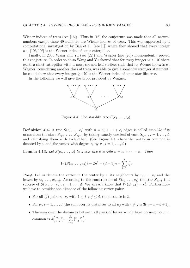
CHAPTER 4. INVERSE PROBLEMS - FORBIDDEN VALUES 80
Wiener indices of trees (see [16]). Thus in [16] the conjecture was made that all naturalnumbers except these 49 numbers are Wiener indices of trees. This was supported by acomputational investigation by Ban et al. (see [1]) where they showed that every integern ∈ [103, 108] is the Wiener index of some caterpillar.
Finally, in 2006 Wang and Yu (see [22]) and Wagner (see [20]) independently provedthis conjecture. In order to do so Wang and Yu showed that for every integer w > 108 thereexists a short caterpillar with at most six non-leaf vertices such that its Wiener index is w.Wagner, considering another class of trees, was able to give a somehow stronger statement:he could show that every integer ≥ 470 is the Wiener index of some star-like tree.
In the following we will give the proof provided by Wagner.
v
v1 v2 vd
Figure 4.4: The star-like tree S(c1, . . . , cd).
Definition 4.4. A tree S(c1, . . . , cd) with n = c1 + · · · + cd edges is called star-like if itarises from the stars Sc1+1, . . . , Scd+1 by taking exactly one leaf of each Sci+1, i = 1, . . . , d,and identifying them with each other. (See Figure 4.4 where the vertex in common isdenoted by v and the vertex with degree ci by vi, i = 1, . . . , d.)
Lemma 4.13. Let S(c1, . . . , cd) be a star-like tree with n = c1 + · · ·+ cd. Then
W (S(c1, . . . , cd)) = 2n2 − (d− 1)n−d∑i=1
c2i .
Proof. Let us denote the vertex in the center by v, its neighbours by v1, . . . , vd and theleaves by w1, . . . , wn−d. According to the construction of S(c1, . . . , cd) the star Sci+1 is asubtree of S(c1, . . . , cd), i = 1, . . . , d. We already know that W (Sci+1) = c2
i . Furthermorewe have to consider the distance of the following vertex pairs:
• For all(d2
)pairs vi, vj with 1 ≤ i < j ≤ d, the distance is 2.
• For vi, i = 1, . . . , d, the sum over its distances to all wj with i 6= j is 3(n− ci−d+1).
• The sum over the distances between all pairs of leaves which have no neighbour in
common is 4((
n−d2
)−
d∑i=1
(ci−1
2
)).

CHAPTER 4. INVERSE PROBLEMS - FORBIDDEN VALUES 81
Altogether we obtain
W (S(c1, . . . , cd)) =d∑i=1
c2i + 2
(d
2
)+ 3
d∑i=1
(n− ci − d+ 1)
+ 4
((n− d
2
)−
d∑i=1
(ci − 1
2
))
=d∑i=1
c2i + d(d− 1) + 3(n− d+ 1)d− 3n
+ 2(n− d)(n− d− 1)− 2d∑i=1
(c2i − 3ci + 2)
= 2n2 − nd− 5n+ 4d−d∑i=1
c2i + 6n− 4d
= 2n2 − (d− 1)n−d∑i=1
c2i .
Lemma 4.14. Let S(c1, . . . , cd) be the star-like tree with n = c1 + · · · + cd. Furthermorelet ci = cj = c for some 1 ≤ i, j ≤ d, i 6= j. Then
W (S(c1, . . . , cd)) > W (S(c′1, . . . , c′d))
for the star-like tree S(c′1, . . . , c′d) with
c′k =
c− 1 if k = i,
c+ 1 if k = j,
ck otherwise.
Proof. Obviously n and d remain unchanged. Thus according to Lemma 4.13 we obtain
W (S(c1, . . . , cd))−W (S(c′1, . . . , c′d)) = (c− 1)2 + (c+ 1)2 − 2c2 = 2 > 0.
Definition 4.5. The star-like tree with c1 = · · · = cl = 2 and cl+1 = · · · = cl+k = 1 isdenoted by S(2l, 1k). Besides we refer to the Wiener index of S(2l, 1k) as w(l, k).
It is easy to see that for S(2l, 1k) we get n = 2l + k and d = l + k. Thus we have
w(l, k) = 2(2l + k)2 − (l + k − 1)(2l + k)− 4l − k = 6l2 + (5k − 2)l + k2.

CHAPTER 4. INVERSE PROBLEMS - FORBIDDEN VALUES 82
l 2 3 4 5 6 7 8 9 10 11 12 13s(l) 1 1 3 4 4 7 9 10 10 14 17 19
l 14 15 16 17 18 19 20 21 22 23 24 25s(l) 20 20 25 29 32 34 35 35 41 46 50 53
Table 4.1: s(l) for all star-like trees S(2l, 1k) with 2 ≤ l ≤ 25.
Definition 4.6. Let S(c1, . . . , cd) be the star-like tree with ci = cj = c for some indices1 ≤ i, j ≤ d, i 6= j. Replacing ci by c+ 1 and cj by c− 1 is called a splitting step.
The number of splitting steps one can perform starting with S(2l, 1k) is denoted by s(l)(which is independent of the number of 1’s occurring in S(2l, 1k)).
Example 4.15. Let us consider the star-like tree S(2l, 1k) with l = 5. Then we canperform the following splitting steps
S(25, 1k) ↪→ S(3, 3, 2, 1k+2) ↪→ S(4, 2, 2, 1k+2) ↪→ S(4, 3, 1k+3).
Thus we have s(5) = 4.A list of all s(l) for 2 ≤ l ≤ 25 is given in Table 4.1.
Obviously s(l) is a non-decreasing function and we have s(l + 7) ≥ s(l) + s(7) ands(l + 8) ≥ s(l) + s(8). Using Table 4.1 we see that s(l) ≥ l + 5 for 12 ≤ l ≤ 18 ands(l) ≥ l + 9 for 16 ≤ l ≤ 24. Thus we obtain s(l) ≥ l + 5 for l ≥ 12 and s(l) ≥ l + 9 forl ≥ 16.
Now, starting with S(2l, 1k), we can construct star-like trees with Wiener index w(l, k),w(l, k)− 2, . . ., w(l, k)− 2s(l) by using splitting steps and applying Lemma 4.14.
Proposition 4.16. For every even integer w ≥ 1506 there exists a star-like tree S(c1, . . . , cd)such that W (S(c1, . . . , cd)) = w.
Proof. Let us consider the star-like tree S(2l, 1k) with k = 0, 2, 4, . . . , 10 and l = x+ 1− k2.
Then according to Lemma 4.13 we obtain
W (l, k) = 6
(x+ 1− k
2
)2
+ (5k − 2)
(x+ 1− k
2
)+ k2
= 6x2 + (10− k)x+ 4.
Let x ≥ 16. Then we have l ≥ 16 + 1− 102
= 12 and therefore
s(l) ≥ l + 5 ≥ l +k
2= x+ 1.
Thus
6x2 + (10− k)x+ 4− 2s(l) ≤ 6x2 + (10− k)x+ 4− 2(x+ 1)
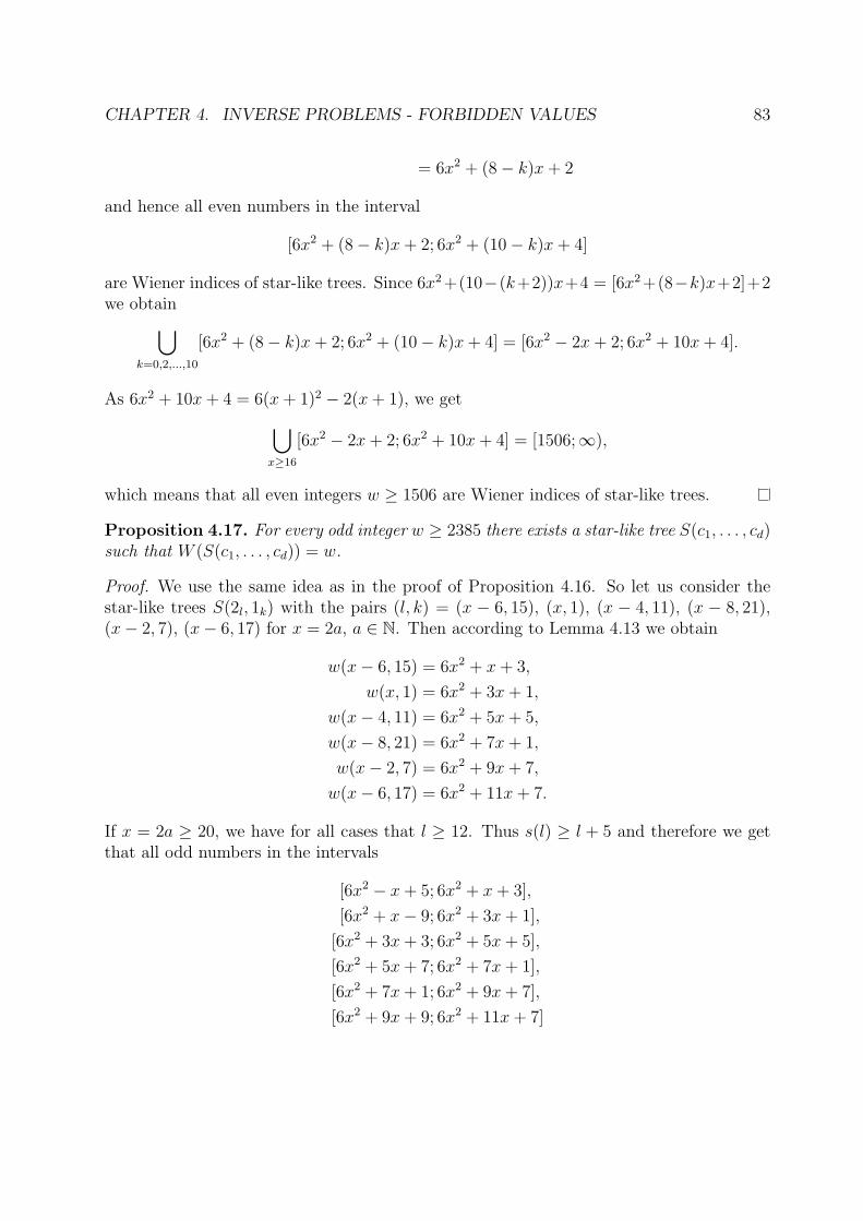
CHAPTER 4. INVERSE PROBLEMS - FORBIDDEN VALUES 83
= 6x2 + (8− k)x+ 2
and hence all even numbers in the interval
[6x2 + (8− k)x+ 2; 6x2 + (10− k)x+ 4]
are Wiener indices of star-like trees. Since 6x2 +(10−(k+2))x+4 = [6x2 +(8−k)x+2]+2we obtain⋃
k=0,2,...,10
[6x2 + (8− k)x+ 2; 6x2 + (10− k)x+ 4] = [6x2 − 2x+ 2; 6x2 + 10x+ 4].
As 6x2 + 10x+ 4 = 6(x+ 1)2 − 2(x+ 1), we get⋃x≥16
[6x2 − 2x+ 2; 6x2 + 10x+ 4] = [1506;∞),
which means that all even integers w ≥ 1506 are Wiener indices of star-like trees.
Proposition 4.17. For every odd integer w ≥ 2385 there exists a star-like tree S(c1, . . . , cd)such that W (S(c1, . . . , cd)) = w.
Proof. We use the same idea as in the proof of Proposition 4.16. So let us consider thestar-like trees S(2l, 1k) with the pairs (l, k) = (x − 6, 15), (x, 1), (x − 4, 11), (x − 8, 21),(x− 2, 7), (x− 6, 17) for x = 2a, a ∈ N. Then according to Lemma 4.13 we obtain
w(x− 6, 15) = 6x2 + x+ 3,
w(x, 1) = 6x2 + 3x+ 1,
w(x− 4, 11) = 6x2 + 5x+ 5,
w(x− 8, 21) = 6x2 + 7x+ 1,
w(x− 2, 7) = 6x2 + 9x+ 7,
w(x− 6, 17) = 6x2 + 11x+ 7.
If x = 2a ≥ 20, we have for all cases that l ≥ 12. Thus s(l) ≥ l + 5 and therefore we getthat all odd numbers in the intervals
[6x2 − x+ 5; 6x2 + x+ 3],
[6x2 + x− 9; 6x2 + 3x+ 1],
[6x2 + 3x+ 3; 6x2 + 5x+ 5],
[6x2 + 5x+ 7; 6x2 + 7x+ 1],
[6x2 + 7x+ 1; 6x2 + 9x+ 7],
[6x2 + 9x+ 9; 6x2 + 11x+ 7]

CHAPTER 4. INVERSE PROBLEMS - FORBIDDEN VALUES 84
are Wiener indices of some star-like trees, which means that all odd numbers in the interval[6x2 − x+ 5; 6x2 + 11x+ 7] for x = 2a ≥ 20 are Wiener indices of some star-like trees.
Now, let us consider the star-like trees S(2l, 1k) with the pairs (l, k) = (x − 1, 3),(x− 5, 13), (x− 9, 23), (x− 3, 9), (x− 7, 19), (x− 1, 5) for x = 2a− 1, a ∈ N. Analogouslywe obtain by Lemma 4.13
w(x− 1, 3) = 6x2 + x+ 2,
w(x− 5, 13) = 6x2 + 3x+ 4,
w(x− 9, 23) = 6x2 + 5x− 2,
w(x− 3, 9) = 6x2 + 7x+ 6,
w(x− 7, 19) = 6x2 + 9x+ 4,
w(x− 1, 5) = 6x2 + 11x+ 8.
If x = 2a− 1 ≥ 21, we have for all cases that l ≥ 12. Thus s(l) ≥ l + 5. Furthermore, forl = x − 3 ≥ 18 we have s(x − 3) ≥ (x − 3) + 90x + 6, and therefore we get that all oddnumbers in the intervals
[6x2 − x− 6; 6x2 + x+ 2],
[6x2 + x+ 4; 6x2 + 3x+ 4],
[6x2 + 3x+ 6; 6x2 + 5x− 2],
[6x2 + 5x; 6x2 + 7x+ 6],
[6x2 + 7x+ 8; 6x2 + 9x+ 4],
[6x2 + 9x; 6x2 + 11x+ 8]
are Wiener indices of some star-like trees, which means that all odd numbers in the interval[6x2 − x− 6; 6x2 + 11x+ 8] for x = 2a− 1 ≥ 21 are Wiener indices of some star-like trees.
Combining those two results, we obtain that for any x ≥ 20 all odd numbers in theinterval
[6x2 − x+ 4; 6x2 + 11x+ 8]
are Wiener indices of some star-like trees. Since 6x2 + 11x + 8 = 6(x + 1)2 − (x + 1) + 3,we obtain ⋃
x≥20
[6x2 − x+ 4; 6x2 + 11x+ 8] = [2384;∞),
which means that all odd integer w ≥ 2384 are Wiener indices of star-like trees.
Furthermore Wagner checked via computer that all integers 470 ≤ w ≤ 2384 are Wienerindices of star-like trees with less then 41 edges. Thus, together with [12], the followingtheorem holds:
Theorem 4.18. Let w ∈ N0. Then there exists a tree T with W (T ) = w if and only ifw ∈ N0 \ {2, 3, 5, 6, 7, 8, 11, 12, 13, 14, 15, 17, 19, 21, 22, 23, 24, 26, 27, 30, 33, 34, 37, 38, 39, 41,43, 45, 47, 51, 53, 55, 60, 61, 69, 73, 77, 78, 83, 85, 87, 89, 91, 88, 101, 106, 113, 147, 159}.

Bibliography
[1] Y.-E. A. Ban, S. Bereg, and N. H. Mustafa. A conjecture on Wiener indices incombinatorial chemistry. Algorithmica, 40(2):99–118, 2004.
[2] D. Bonchev and D. J. Klein. On the Wiener number of thorn trees, stars, rings, androds. Croatica Chemica Acta, 75:613–620, 2002.
[3] E. R. Canfield, R. Robinson, and D. H. Rouvray. Determination of the Wiener molec-ular branching index for the general tree. J. Comput. Chem., 6:598–609, 1985.
[4] A. Dobrynin. Branchings in trees and the calculation of the Wiener index of a tree.MATCH Commun. Math. Comput. Chem., 41:119–134, 2000.
[5] A. Dobrynin, R. Entringer, and I. Gutman. Wiener index of trees: theory and appli-cation. Acta Appl. Math., 66:211–249, 2001.
[6] A. Dobrynin and I. Gutman. On a graph invariant related to the sum of all distancesin a graph. Publ. Inst. Math. (Beograd), 56:18–22, 1994.
[7] J. Doyle and J. Graver. Mean distance in a graph. Discrete Math., 17:147–154, 1977.
[8] R. Entringer, D. Jackson, and D. Snyder. Distance in graphs. Czechoslovak Math. J.,26:283–296, 1976.
[9] M. Fischermann, A. Hoffmann, D. Rautenbach, L. Szekely, and L. Volkmann. Wienerindex versus maximum degree in trees. Discrete Applied Mathematics, 122:127–137,2002.
[10] I. Gutman. Distance of thorny graphs. Publ. Inst. Math. (Beograd), 63:31–36, 1998.
[11] I. Gutman and Y.-N. Yeh. The sum of all distances in bipartite graphs. MathematicaSlovaca, 45:327–334, 1995.
[12] I. Gutman, Y.-N. Yeh, and J.-C. Chen. On the sum of all distances in graphs. TamkangJ. Math., 25:83–86, 1994.
[13] M. Hazewinkel, editor. Encyclopaedia of mathematics. Kluwer Academic Publishers,2002. An online version can be found at http://eom.springer.de/default.htm.
85

BIBLIOGRAPHY 86
[14] N. Jacobson. Basic algebra I. W. H. Freeman and company (San Francisco), 1974.
[15] W. Kocay and D. L. Kreher. Graphs, algorithms, and optimization. Chapman andHall / CRC, 2005.
[16] M. Lepovic and I. Gutman. A collective property of trees and chemical trees. J. Chem.Inf. Comput. Sci., 38:823–826, 1998.
[17] R. Merris. An edge version of the matrix-tree theorem and the Wiener index. Linearand Multilinear Algebra, 25:291–296, 1989.
[18] O. E. Polansky and D. Bonchev. The Wiener number of graphs. I. General theory andchanges due to some graph operations. MATCH Commun. Math. Comput. Chem.,21:133–186, 1986.
[19] R. Shi. The average distance of trees. Systems Sci. Math. Sci., 6:18–24, 1993.
[20] S. G. Wagner. A class of trees and its Wiener index. Acta Appl. Math., 91:119–132,2006.
[21] H. Wang. The extremal values of the Wiener index of a tree with given degree sequence.Discrete Applied Mathematics, 156:2647–2654, 2008.
[22] H. Wang and G. Yu. All but 49 numbers are Wiener indices of trees. Acta Appl.Math., 92:15–20, 2006.
[23] H. Wiener. Structural determination of paraffin boiling points. J. Amer. Chem. Soc.,69:17–20, 1947.
[24] B. Zelinka. Medians and peripherians of trees. Arch. Math. (Brno), 4:87–95, 1968.
[25] X.-D. Zhang, Y. Liu, and M.-X. Han. The maximum Wiener index of trees with givendegree sequences. Preprint, arXiv:0907.3772v1, July 2009.