The Weekend Effect in Equity Option Returns ∗

Christopher S. Jones Joshua ShemeshMarshall School of Business Department of Finance

University of Southern California University of Melbournechristopher.jones@marshall.usc.edu joshua.shemesh@unimelb.edu.au

August 30, 2012

Abstract

We find that returns on options on individual equities display markedly lower returns overweekends (Friday close to Monday close) relative to any other day of the week. These patternsare observed both in unhedged and delta-hedged positions, indicating that the effect is not theresult of a weekend effect in the underlying securities. Our results hold for puts and calls overa wide range of maturities and strike prices and remains strong in samples that include onlythe most liquid options. We find no evidence of a weekly seasonal in bid-ask spreads, tradingvolume, or open interest that could drive the effect. We also do not find evidence that weekendreturns are significantly risker than weekday returns, though the weekend effect does appearstronger when the riskiness of the market portfolio is high. Weekend returns are lower when theTED spread and market volatility are high, suggesting that limits to arbitrage may explain thepersistence of the effect.

∗We are grateful for comments from Mike Chernov, Larry Harris, Robert Hudson, Nikunj Kapadia, Oguz Ozbas,Yigal Newman, Nick Polson, Allen Poteshman, Eric Renault, Mark Weinstein, Fernando Zapatero, and seminarparticipants at USC, Hebrew University, the 2009 Montreal Financial Econometrics Conference, the 2009 FinancialManagement Association meetings, and the 2010 American Finance Association meetings. Shemesh thanks theSanger Chair of Banking and Risk Management for financial support.

1 Introduction

The weekend effect in the stock market represents one of the earliest and most studied pieces

of evidence against the Efficient Market Hypothesis, yet the effect has received little attention

in recent literature. The explanation seems to be that the weekend effect has disappeared, at

least in equity markets, sometime during the last two decades. Why the effect disappeared,

or whether there ever was a weekend effect to begin with, as Sullivan, Timmermann, and

White (2001) have questioned, remain open questions.

Although the modern weekend effect literature began with the article of French (1980),

evidence on the effect was reported 50 years earlier by Fields (1931). Similar effects have

been observed in international equity indexes (e.g. Jaffe and Westerfield (1985)), in a variety

of government bond returns (e.g. Gibbons and Hess (1981), Flannery and Protopapadakis

(1988)), and in U.S. equities as far back as 1885 (Bessembinder and Hertzel (1993)). The

robustness of the finding was short-lived, however, as authors such as Connolly (1989) and

Chang, Pinegar, and Ravichandran (1993) suggested that the effect started disappearing in

the 1970s or 80s. Kamara (1997) showed that the disappearance happened the soonest for

the largest firms. Chen and Singal (2003) argued that it is the introduction of options on a

firm’s stock that led to the elimination of the weekend effect in a specific firm. Since options

tended to be introduced first for large capitalization firms, this offers a potential explanation

of Kamara’s result.

The Chen and Singal (2003) finding deserves further investigation because it implies that

the weekend effect may not have disappeared, but merely changed addresses. Their story is

actually related to the original intuition of Fields (1931), who conjectured that risk-averse

equity investors might want to close out their positions on Friday afternoon and open them

back up on Monday morning. Chen and Singal modify this intuition by suggesting that it

is the short sellers that are most interested in closing positions before the weekend. Their

reasoning is simple – with unbounded downside risk, naked short positions require constant

monitoring, which becomes difficult if not impossible to perform over the weekend.

1

Chen and Singal (2003) support their hypothesis with the observation that the weekend

effect was most pronounced in stocks with high levels of short interest and the finding that

the weekend effect disappeared only for those stocks on which options are traded. Their

result is also consistent with the decline in the weekend effect for US Treasuries, for which

derivative products are widely used.

The same intuition implies another effect that remains unexplored. If investors are gen-

erally averse to holding positions with unbounded risk over the weekend, then speculators

who have written call option positions should also attempt to close out these positions unless

they receive additional compensation for that risk in the form of declining option premia.

Put option writers, while not exposed to a completely unbounded risk, still face the possi-

bility of losses that are far in excess of those that likely to occur in an equity position, for

example. For this reason we believe that the Chen and Singal (2003) hypothesis has the

straightforward implication that we should see a weekend effect in call and put options, with

weekend option returns being substantially lower than returns over the rest of the week.

We view this story only as one possible motivation for examining weekday effects in

equity option markets. More generally, options represent one of the last unexplored asset

classes for assessing the survival of the weekend effect. Knowing whether or not such an

effect exists has substantial implications for a number of literatures. Besides providing an

additional test of the Chen and Singal (2003) hypothesis, an unambiguous result from the

options market would directly address the view of Sullivan, Timmermann, and White (2001)

that the weekend effect was most likely the result of data mining.

Finding a weekend effect in option returns might also provide a new direction for the

option pricing literature in its search for models capable of explaining upward-sloping term

structures and smile-shaped cross sections in Black-Scholes implied volatilities. This liter-

ature is divided over the importance of jumps versus stochastic volatilities and the correct

risk premia to attribute to each (e.g. Pan (2002), Broadie, Chernov, and Johannes (2007)).

A weekend effect in option returns would indicate that the risks that are more prevalent or

less manageable over the weekend are the ones that require the largest risk premia.

2

We look for a weekend effect in option returns using simple methods. Using the Op-

tionMetrics dataset over the period from January 1996 to June 2007, we form portfolios of

options. Portfolios are formed on the basis of option maturity, moneyness, or both. Puts and

calls are put in different portfolios. We experiment with a variety of sampling and weighting

schemes. In addition, we examine returns separately for each year in our sample period.

The results are clear cut. The weekend effect in individual equity option returns is large

and negative. We observe the effect in unhedged returns, but an analysis of delta-hedged

returns suggests that little of the effect is due to any weekend effect in the underlying stock

returns. All results are highly statistically significant, often with t-statistics exceeding 10.

We find similar effects in puts and calls and across almost all maturity and moneyness

categories.

After an adjustment to quote implied volatilities in terms of trading time rather than

calendar time, we find a weekly seasonal in implied volatilities that is even more significant

than that of the option returns. We also examine a measure we refer to as “total implied

volatility”, which is simply the Black-Scholes implied volatility of the stock price at expi-

ration, not reported per unit of time. As an option moves closer to expiration, it’s total

volatility tends to decrease as the length of time before expiration decreases. Over the week-

end, total implied volatility declines over twice as much as any other day of the week, which

is inconsistent with the observation, first made by French and Roll (1986) and confirmed in

our sample below, that the actual volatility of Friday close to Monday close returns is no

greater than the volatility of returns over any other close-to-close interval.

Our results are unaffected when we restrict the sample to the most liquid options and to

options on firms that are members of the S&P 100. We do not, however, find strong evidence

of a weekend effect in S&P 500 Index options.

We investigate a number of potential explanations for the effect. One is that our results

are due to data mining, a concern articulated by Sullivan, Timmermann, and White (2001).

Another is that the margins required to write options are more costly to maintain over the

weekend than during the week. Although the underlying equity returns do not appear any

3

riskier over the weekend, we do find limited evidence that option returns are slightly more

volatile, suggesting that higher risk may be partly responsible for the effect. We do not

find evidence that our results can be attributed to the biases that result from measurement

errors in prices, as in Blume and Stambaugh (1983). Finally, we find no evidence or weekly

patterns in volume or open interest that might suggest other liquidity-based explanations of

our results.

Regressions reveal that the effect is substantially stronger for expiration weekends (week-

ends that follow the last day of trading for front month contracts). It appears to exist to a

lesser extent for mid-week holidays as well, though the evidence for this finding is weaker,

most likely because of low incidence of mid-week holidays. In addition, the weekend effect is

more negative in times when S&P 500 Index volatility and the TED spread are high. Since

higher values of these two variables should make arbitrage strategies more difficult to imple-

ment, we interpret these findings as providing evidence for a limits to arbitrage explanation

as to why the effect persists.

We know of only one other paper, Sheikh and Ronn (1994), that investigates weekly

patterns in options markets. In examining short-term at-the-money options on 30 stocks

over a period of just 21 months, Sheikh and Ronn find some evidence of a weekly seasonal

in which call returns are highest on Wednesdays, but they do not find a weekend effect in

calls or in puts. Furthermore, after adjusting option returns by subtracting Black-Scholes

model-implied returns, the pattern in calls disappears, though a significant weekend effect

arises in adjusted put returns. Our paper therefore resolves the ambiguity of their findings,

showing that weekend effects are present in both calls and puts over a far more extensive

sample.

The paper is organized as follows. In Section 2 we describe our data, sampling methods,

and portfolio construction. Section 3 contains results that document weekly patterns in

returns, implied volatilities, and liquidity measures. Section 4 examines the determinants of

weekend and weekday returns in a regression setting. Section 5 concludes.

4

2 Data and methods

Our primary data source is the Ivy DB data set from OptionMetrics. This data set includes

all US listed options on equities, indexes, and ETFs. In our paper we generally restrict our

attention to individual equity options, though for a few results we examine S&P 500 Index

options.

Throughout our analysis, we form portfolios of options on the basis of maturity and/or

delta. The delta we use is lagged an extra day, i.e. if we are forming a portfolio at day t− 1

to hold until day t, then we use the delta that was observed on day t− 2. We do this so that

if there are measurement errors in deltas they are not correlated with the returns on the

same assets. We consider five maturity ranges and six delta ranges so that all options in a

given portfolio are at least roughly comparable and all portfolios have a reasonable number

of options included. Finally, we have separate portfolios for calls and puts.

We compute portfolio returns by taking the equal or value weighted average of the returns,

either hedged or unhedged, of each option in that portfolio. Since our dataset includes bid-

ask quotes rather than transaction prices, we compute returns from quote midpoints. Since

options have zero net supply, the concept of value weighting must be reinterpreted, and what

we call value weighted portfolios are actually weighted by the dollar value of open interest

for each option. We usually examine excess returns, where we compute riskless returns using

the shortest maturity yield provided in the Ivy DB zero curve file.

We impose a number of filters to try to eliminate a number of sources of noise. We find

many large errors on the first day an option is introduced, so we exclude the first observation

for each contract. Large return reversals (2000% followed by -95% or vice versa) are also

eliminated. Because large bid-ask spreads are likely to be less informative, and to deal

with obvious data errors, we exclude the day t return on an option if any of the following

conditions hold:

• day t− 2 bid price is less than $0.50 or 0.1% of the price of the underlying stock

5

• day t− 2 bid-ask spread is more than 25% of the midpoint

• day t− 1 or t bid-ask spread is more than $5.00 or 200% of the midpoint

• day t−1 or t ask price is less than the bid or more than twice the price of the underlying

stock

The first two conditions represent filters that are implemented prior to the return interval.

These focus our attention away from the least liquid segment of the options market, which

tends to be deep out-of-the-money contracts. Note that if the day t − 2 values that these

filters are based on are measured with error, then this error should at least be uncorrelated

with the subsequent return from day t − 1 to t. The last two conditions are included to

eliminate a small number of major outliers that we do not catch otherwise. These might be

data recording errors or non-competitive “stub” quotes posted by a market maker who does

not want to trade. We also eliminate quotes in which the bid or ask is set to what appears

to be an undocumented missing value code (e.g. 999). Finally, we eliminate observations in

which there was a stock split between day t− 1 and day t. Together, these filters eliminate

the largest and most suspicious outliers in our sample. We note, however, that all of our

main results are robust to dropping all of these filters.

The implied volatilities in our analysis are provided by Ivy DB (with some adjustments

we describe below). They are computed using a binomial tree approach that accounts for

dividends. (Because they are equivalent to Black-Scholes values for stocks that pay no

dividends, we will refer to the implied volatilities and Greeks as “Black-Scholes” values.)

The delta of each option is also computed with the Black-Scholes model using the implied

volatility from that same option.

In many cases the OptionMetrics database does not include an implied volatility. Most

often, this is because an option contract appears to have negative intrinsic value, making

the implied volatility undefined. As discussed by Battalio and Shultz (2008), apparent

arbitrage opportunities in options data are typically the result of microstructure issues and

measurement errors. If we were to discard options with negative intrinsic values, we would

6

be systematically excluding options with observed prices that are below their true values.

Duarte and Jones (2008) demonstrate that this will result in an downward bias for option

returns.

The solution proposed by Duarte and Jones is to “fill in” missing implied volatilities

with those of similar contracts. If a call option’s implied volatility is missing, then we use

the implied volatility of the put contract written on the same underlying firm with the same

maturity and strike price. If both put and call implied volatilities are missing, then we use the

value from the same contract on the previous day. It is worth noting that this procedure of

filling in missing implied volatilities relies only on current and lagged information. A portfolio

strategy that uses the implied volatilities from this procedure for portfolio formation and for

computing hedge ratios is therefore fully implementable.

Option returns and excess returns are defined as

Ct − Ct−1

Ct−1

andCt − Ct−1

Ct−1

− rt−1NDt−1,t,

respectively, where Ct is the option bid-ask midpoint, rt is the riskless return per day, and

NDt−1,t is the number of calendar days between date t− 1 and t. Given that the change in

value of a delta-hedged portfolio is

Ct − Ct−1 −∆(St − St−1) ,

we define delta-hedged returns as

Ct − Ct−1

Ct−1

−∆St−1

Ct−1

St − St−1

St−1

and delta-hedged excess returns as

Ct − Ct−1

Ct−1

− rt−1NDt−1,t −∆St−1

Ct−1

(

St − St−1

St−1

− rt−1NDt−1,t

)

.

7

This may be viewed as the excess return on a portfolio that combines one option contract

with a zero-cost position in ∆ shares worth of single-stock futures.

We view our use of the Black-Scholes model as relatively benign. Even if the delta we use

to compute hedged returns is incorrect, those hedged returns nevertheless represent the re-

turns on a feasible investment strategy (abstracting from transactions costs). Delta hedging,

while not perfect, can be expected to remove at least the majority of the option’s exposure to

the underlying stock. Hull and Suo (2002) claim, in fact, that Black-Scholes works about as

well as any other model in this regard. When we examine weekday effects in Black-Scholes

implied volatilities, our results may also be slightly skewed by model misspecification. Nev-

ertheless, it is hard to imagine how this form of misspecification could causes systematic

patterns across different days of the week.

Summary statistics describing our sample are included in Table 1. The table examines the

excess returns on equal weighted portfolios of unhedged and delta-hedged option positions,

where portfolios are formed on the basis of option delta.

Several stylized facts are immediately apparent. First, portfolios of unhedged call options

have positive average returns, while unhedged puts have negative average returns, which is

consistent with calls having positive market betas and puts having negative betas. Second,

all portfolios of unhedged option positions have returns that display positive skewness and

substantial excess kurtosis. Delta-hedged option returns are even more fat-tailed. This is the

result of delta hedging being more effective for small changes in stock prices. Large changes

in stock prices, which are often the source of extreme option returns, cannot be hedged due

to the convexity of option payoffs. We also see a systematic relation between moneyness

and volatility. Out-of-the-money (OTM) options are substantially more risky than in-the-

money options. This is the direct result of OTM options representing more highly leveraged

exposures to the underlying securities.

Another regularity in Table 1 is that average delta-hedged returns are almost all positive,

for most option deltas and for both puts and calls. We believe that these positive means

are likely the result of an upward bias arising from measurement errors in observed prices.

8

This bias, discussed first by Blume and Stambaugh (1983) and more recently by Duarte and

Jones (2008), is a significant problem when measuring average returns. We believe that our

results, which focus on the differences between Monday and non-Monday returns, should be

unaffected by this bias. Nevertheless, we address the issue below in Section 4.1.

Finally, Table 1 contains the average number of options in our sample and in each delta-

sorted portfolio. Our sample contains, on a typical day, almost 60,000 contracts, representing

several dozen puts and calls of different deltas and maturities for the average firm. Portfolios

that are formed on the basis of delta are generally well populated, usually containing 5,000

contracts or more. A few portfolios, namely the deep out-of-the-money puts and calls,

contain many fewer contracts. As discussed above, this is the direct result of the data filters

we impose. The contracts that pass our filters and remain in these portfolios, while limited

in number, should hopefully provide a more accurate assessment of the performance of deep

OTM contracts.

3 Weekday patterns in option markets

3.1 Main findings

Our main results are presented in Tables 2-A and 2-B. Table 2-A displays average excess

returns across different days of the week on portfolios of puts and calls sorted by delta.

When we average across all options, both puts and calls, we see an average Monday return

of -0.58%, indicating that the average option loses more than half of 1% of its value each

weekend. The corresponding t-statistic is -16.1 The average returns for other days of the

week are all positive. Similar results are obtained for portfolios of puts or calls that are sorted

on delta. Monday returns are in all cases negative, though their statistical significance is

sometimes only marginal.2

1 All tables report asymptotic t-statistics. We have also computed p-values for all our key results using bootstrapdistributions, and we find these results to be essentially identical. Additional nonparametric results, reported inSection 3.6, also addresses finite sample issues.

2 The higher levels of statistical significance for the pooled portfolio of unhedged puts and calls is due to thereduction in variance that comes from the offsetting deltas of puts and calls, which has approximately the same effect

9

Table 2-B presents corresponding results for delta-hedged excess returns. A subset of

these results is reported graphically in Figure 1. These results show that delta-hedged returns

exhibit an even stronger weekend effect with markedly increased statistical precision. This

suggests two conclusions. One is that the weekend effect in option returns is not the result

of a weekend effect in the underlying stocks. If it was, then delta hedging would eliminate

at least the majority of that weekly pattern. Second, delta-hedged returns are substantially

less volatile than unhedged returns, so standard errors on average hedged returns are much

smaller.

Because we observe the same effect in delta-hedged returns, and because we see that

effect much more clearly, our subsequent analysis will be focused on delta-hedged positions.

In addition, we simply feel that looking at delta-hedged returns is also more interesting.

The literature has already examined weekend effects in stock returns, so if delta hedging at

least substantially eliminates the portion of the option return that is due to the underlying

stock, then whatever returns remain should reflect risks that have thus far received much

less attention in the literature.

Table 3 performs the same analysis on delta-hedged excess returns, only now the portfolios

are sorted on the basis of maturity rather than delta. Here we see that the effect is strong

for all maturities except the longest. Even the 1-10 day maturity range, which many studies

discard because of expiration-day concerns, displays the weekend effect strongly.

The results in Tables 2-3 demonstrate large negative and highly significant Monday re-

turns, but they are not completely satisfactory for three reasons. First, they do not directly

assess the statistical significance of the differences between average returns on different days

of the week, which would represent the most direct evidence of a weekend effect. Second, the

presence of Monday holidays means that weekend returns are sometimes not observed until

Tuesday, so the interpretation of Monday returns as weekend returns is not always correct.

Finally, in order to present these results in a reasonable amount of space we are limited

to one-way sorts on the basis of either maturity or delta, resulting in highly aggregated

as delta hedging.

10

portfolios whose constituents may differ widely.

To address all three of these issues, we next examine the differences between weekend

and non-weekend returns for portfolios sorted on the basis of both maturity and delta, where

the weekend return is defined as the return from the last trading day of one week to the

first trading day of the next. The results, presented in Table 4, show that average returns

are lower over weekends for almost all portfolios, and most of these results are statistically

significant at very high confidence levels. For the disaggregated portfolios of both calls and

puts, average differences range from around zero to more than -3%, with the typical portfolio

having an average difference of about -1%.

A potential concern is that our returns are calculated assuming no early exercise. Early

exercise can be optimal for put options and, in the case of stocks about to pay dividends,

for call options as well. In these cases, our computed returns should understate the returns

to a portfolio in which exercise decisions are made optimally. For puts, the value of early

exercise comes from the possible benefit of accelerating the fixed option premium forward in

time. While this can have a significant effect on option value, the loss in value that results

from delaying exercise by one day should be small, as it is at most the loss of one day of

interest on the option payoff.

For calls, failing to exercise prior to a large dividend could have a substantial effect on

the one-day option return. This cannot explain our results for two reasons. First, firms do

not have any tendency to go ex dividend over the weekend, with Wednesdays and Thursdays

containing about 60% of all ex dividend dates in our sample. Thus, if failing to account for

early exercise is biasing any of our average returns downward, it is the non-weekend returns,

so accounting for early exercise would only magnify the difference between weekend and

weekday returns.

Most importantly, early exercise cannot explain our results because it is only optimal for

call and put options that are significantly in the money. Since we find large weekend effects

across all moneyness levels, early exercise due to dividends or any other factor cannot be a

primary explanation of our findings.

11

3.2 Weekday effects in other variables

Table 5-A looks at weekday effects in other variables to determine whether we see effects that

are consistent with those found in equity option excess returns. We first examine “simple”

returns, which are identical to the returns we examined previously but do not subtract the

riskless rate. We start with simple returns to exclude the possibility that our results arise

from the way we are computing riskless returns. Averages of simple unhedged and delta-

hedged returns, shown in the top rows of the table, demonstrate the same weekly patterns

that we observed for excess returns. Thus, the weekend effect in excess returns cannot

simply be attributed to the fact that excess returns over weekends are reduced by three days

of riskless return.

We next investigate average changes in several different measures of implied volatility.

While changes in implied volatilities would seem somewhat mechanically related to option

returns, it is not necessarily the case that patterns in returns and implied volatilities will

mirror each other. As a simple example, consider the case in which investors are risk neutral

and volatility changes deterministically. In this case, changes in implied volatilities will be

predictable, but all expected excess returns are zero. A model that generates an effect in

returns, as we have observed, but not in implied volatilities is somewhat more difficult to

construct but is nevertheless a theoretical possibility.3

Table 5-A reports results for three different measures of implied volatility. The first is the

“unadjusted” implied volatility that is provided in Ivy DB. This measure of volatility tends

to rise as options approach expiration, most likely reflecting a misspecification of the Black-

Scholes model. Surprisingly, however, we see that the rise is greatest on Mondays. While

such a result is theoretically possible, it is nevertheless unintuitive that implied volatility

could rise, indicating higher option values, when returns are most negative.

The answer to this apparent contradiction is in how Ivy DB computes implied volatilities.

In the Black-Scholes formula, it is the total amount of volatility until the expiration date

3 One possibility is a stochastic volatility model in which opposite weekly seasonals in the volatility drift and thevolatility risk premium offset to produce no seasonal in the risk neutral volatility process.

12

that determines option value, not the amount of volatility per unit of time. In other words,

every place the volatility parameter σ appears it is multiplied by the square root of the time

to expiration. Ivy DB measures the time to expiration in terms of calendar time, so that

Monday has three days less time to maturity than the Friday that immediately preceded

it. There is nothing incorrect about this approach – quoting in terms of calendar time is

just a convention – but the interpretability of this convention is slightly problematic. The

reason is that the interval from Friday close to Monday close is about as volatile as any other

close-to-close period, as demonstrated by French and Roll (1986). It certainly is not more

volatile by a factor of√3, which is what we would expect if weekends and weekdays were

equally risky. Hence, when the time to maturity declines by three days but only one day of

actual volatility actually accrues, implied volatility appears to rise.

We address this in two ways. First, we adjust the implied volatility so that it is quoted

in terms of trading days rather than calendar days. Second, we examine “total implied

volatility”, which is the implied volatility of the log stock price at expiration, not reported

per unit of time. This is computed simply by taking the product of the unadjusted implied

volatility and the square root of the time to expiration (measured in calendar time). With

both of these modifications, we see highly significant changes in implied volatility that are

lower on Mondays than they are for the rest of the week.

Finally, we also look for a weekend effect in S&P 500 Index options. Intuitively, one might

expect index options to be driven by the same systematic risk factors that affect individual

equity options. However, the two differ significantly in that index options are options on a

portfolio rather than a portfolio of options. They are therefore affected by correlations as well

as volatilities. Risk factors that drive correlations, as in the model of Driessen, Maenhout,

and Vilkov (2009), should therefore affect only options on the index.

On the other hand, systematic movements in average idiosyncratic volatility will affect

portfolios of individual options but will have little effect on options on the index. Such

systematic movements have been documented by Campbell, Lettau, Malkiel, and Xu (2001)

and have been found by Goyal and Santa-Clara (2003) to drive aggregate risk premia. If the

13

risk premium on this factor has a weekly seasonal, then this will generate a weekend effect

only in individual equity options.

Our results for S&P 500 options, reported in Table 5-B, are somewhat inconclusive. The

average Monday return on the portfolio of all puts is significantly negative and is lower than

the average return over the rest of the week. However, the average Friday return on the

same portfolio is also low, suggesting that Monday returns are not special. Furthermore,

there is no weekend effect observed at all for index call options. Finally, more disaggregated

portfolios, which we do not report in the table, yield weak or nonexistent effects.

3.3 Midweek holidays, long weekends, and expiration weekends

Having established that weekend returns are significantly different from weekday returns, we

now examine midweek holidays, long weekends, and expiration weekends. If the weekend

effect is related to non-trading, then we should also see negative option returns over midweek

holidays, and we might also expect that the effect would be stronger over long weekends.

We also examine whether expiration weekends are different from non-expiration weekends.

Early studies by Stoll and Whaley (1986, 1987) documented that expiration weekends were

associated with higher than normal levels of trading volume, as well as some evidence of

unusual price behavior in the underlying index. More recently, Ni, Pearson, and Poteshman

(2005) document that returns on underlying stocks over expiration weekends appear to be

altered by price manipulation and hedge rebalancing. By controlling for expiration weekends

we can confirm that our finding is not simply driven by option expirations, which also occur

on weekends, but is in fact related to weekend non-trading in general.

We investigate these issues in a regression framework. In all the regressions we run, the

dependent variable is the excess return on a portfolio of delta-hedged option positions. We

consider both equal weighted and value weighted portfolios, where value weighted (VW)

portfolios weight contacts by the dollar value of their open interest. In every case, the unit

of observation is a portfolio, either of puts or calls, that is formed on the basis of a double

14

sort on both delta and maturity.

The independent variables in these regressions consist of four dummy variables. The

first is set to one if the return is computed over any interval that includes a non-trading

period. These are, of course, most often weekends, but they include mid-week holidays as

well. The second dummy is set to one if the non-trading period is a mid-week holiday. This

variable therefore represents the incremental effect of the non-trading period being a mid-

week holiday. The third dummy variable is equal to one if the non-trading period is a long

weekend of three or more days. As with the previous variable, this represents a incremental

effect rather than the total effect of the three-day weekend on returns. Finally, we include a

dummy variable that is equal to one if the return interval includes an expiration weekend.

Again, the coefficient on this variable captures the incremental effect of expiration over and

above the effect that comes from the fact that expiration takes place over the weekend.4

All regressions use ordinary least squares and pool all observations of all double-sorted

portfolios of puts and calls. Because of significant cross-correlations, standard errors are

clustered by date. The so-called Rogers clustering we use also adjusts the standard errors

for conditional heteroskedasticity. In addition, to account for portfolio-level heterogeneity,

we include portfolio fixed effects. This has virtually no effect on any of our results except to

increase the R-squares.

In addition to regressions based on the full sample, we also report results based on more

liquid subsamples. In one pair of regressions, we only include options on stocks that are

members of the S&P 100. In another pair, we only include option contracts that had positive

trading volume for five days in a row prior to the day on which the return is computed. In

both cases, the additional filter has the effect of concentrating the sample on the most liquid

options in the market. Results that use these filters should alleviate concerns that our results

are driven solely by illiquid contracts that do not trade.

Table 6 contains the results of these regressions. In every case, the non-trading dummy

4 We note that expiring options do not have market prices on the Monday following expiration weekend, soour regressions only include options that are not expiring. The dummy variable therefore represents the effect ofexpiration weekend on non-expiring contracts.

15

is highly significant, with t-statistics ranging from 3.76 to 8.92 in absolute value. The size

of the effect is fairly consistent across specifications as well, with non-trading periods having

returns that are lower by about one percent. The results for value weighted portfolios are

moderately weaker than those of the equal weighted portfolios, and the effect in the more

liquid subsamples is just slightly reduced from the full sample, but for all portfolios the

non-trading dummy remains highly significant.

The fact that the non-trading dummy is significant even when the expiration weekend

dummy is included implies that the weekend effect is not simply driven by the fact that expi-

rations take place over the weekend. However, the expiration weekend dummy is significant

in all regressions, suggesting that expiration does have an incremental effect over and above

the effect that comes from non-trading. The expiration effect is stronger for value weighted

relative to equal weighted portfolios, and it is also stronger in the more liquid subsamples.

The fact that the expiration effect is stronger in contracts that are more widely held suggests

the possibility that new option purchases by holders of expiring contracts might result in

high closing prices going into expiration weekend.

The coefficient on the mid-week holiday dummy is only significant for the equal weighted

portfolios from the full sample, but its positive sign suggests that mid-week holidays are

significantly different from weekends. Specifically, mid-week holidays have average returns

that are not as negative as weekends, consistent with the fact that mid-week holidays usually

represent a non-trading period that is just half as long as a regular weekend. The long

weekend dummy is never significant, possibly the result of usually having a small number of

extended weekends each year.

The bottom of the table reports sums of some of the coefficients as well as t-statistics for

those sums. These sums represent the total effect of having a mid-week holiday or a long

weekend rather than the incremental effect over and above the generic non-trading effect.

The results here are not always significant, again probably due to the low numbers of mid-

week holidays and long weekends. Despite the small sample sizes, however, we can still reject

in half the cases that the total effect of a mid-week holiday is zero. This suggests that our

16

findings are more accurately described as a “non-trading” rather than “weekend” effect.

3.4 Robustness

We now ask whether these results are sensitive to changes in our empirical approach. Tables

7-A and 7-B replicate 2-A and 2-B but, instead of equal weighting, weight options by the

dollar value of their open interest. Weighting by open interest has two purposes. One is

that it puts more emphasis on contracts that are likely more liquid and more representative

of the options market as a whole. Second, it should reduce the measurement error bias

identified by Blume and Stambaugh (1983), though this is a bit uncertain since the the bias

in delta-hedged returns is somewhat more complex than the bias in simple returns, as noted

by Duarte and Jones (2008).

Overall, Tables 7-A and 7-B show that average Monday returns are only slightly smaller

for value weighted portfolios than they are for equal weighted portfolios. T-statistics are

generally about the same as those from equal weighted portfolios, more so for delta-hedged

returns. This indicates that negative weekend returns are pervasive in contracts that are

widely held, and not just in puts and calls that exist only on paper.

However, average returns on non-Mondays are noticeably different from results under

equal weighting. In Table 2-B, for instance, we saw significantly positive non-Monday re-

turns for most portfolios of delta-hedged calls and puts. Once combined with the negative

Monday returns, the non-Monday returns were sufficiently positive such that cumulative

weekly returns were positive as well, indicating that the simple strategy of delta-hedging

long option positions would result in high positive rates of return. In contrast, Table 7-B

shows that there is little evidence of systematically positive non-Monday returns, and the

cumulative weekly returns implied from Table 7-B are generally close to zero or slightly

negative.

We believe that the most likely explanation of the differences between equal weighted and

value weighted non-Monday returns is a reduction in the Blume-Stambaugh bias, and that

17

the positive non-Monday returns in Table 2-B were most likely spurious. Since our finding

of significant negative Monday returns is, in contrast, robust to the weighting scheme, we

find it unlikely that it could be driven by the same bias. Nevertheless, we will return to the

issue briefly in Section 4.1.

An alternative robustness check is to alter our sample selection approach to focus on the

most liquid contracts in the market. As in Table 6, we report results based on (i) options

on firms that are members of the S&P 100 and (ii) options that had positive trading volume

for five days in a row prior to the day on which the return is computed.

The results, reported in Table 8, confirm our earlier conclusion that the weekend effect is

not simply a figment of thinly-traded contracts. In particular, the results for the S&P 100

sample are about the same as those from the sample of all firms. For the sample of contracts

with five consecutive days of positive volume, our main result is unaffected and possibly even

stronger than before.

Finally, we move in the opposite direction and include all options in the data set, even

those that we previously filtered out because of large price reversals or bid-ask spreads. In

this sample, all average returns are higher, a result we attribute to the upward bias in average

returns that results from larger measurement errors. Nevertheless, in this sample Monday

returns are still the lowest, generally by the same margin as before.

3.5 Subsample results

In Table 9 we examine each year in our sample separately. We do so for several reasons.

First, finding a consistent effect across years would indicate that our finding is robust and

unlikely to be the result of data mining. Second, if we find that our weekend effect persists

in years, like 2002 and 2003, when both interest rates and interest rate spreads were close to

zero, then it is unlikely that the effect can be attributed to the costs of maintaining margin

requirements, which might be higher over the weekend.

The findings are amazingly consistent across years. In every year, the average return

18

on all options is significantly negative on Mondays. Some Tuesdays are also significantly

negative, but with much less regularity. Notably, the average returns are about as negative

in 2002 and 2003 as they are in the rest of the sample. Figure 2 shows that during this period

T-bill yields were extremely low, and the TED spread (3-month Eurodollars minus 3-month

T-bills) was stuck below 25bps. If the cost of maintaining margin is related to interest rates

or interest rate spreads, then that cost cannot explain the weekend effect in options, at least

completely.

3.6 Nonparametric tests

Thus far, all of our test statistics have been computed based on asymptotic approximations.

In a recent paper, Broadie, Chernov, and Johannes (2009) find that asymptotic standard

errors can be misleading when applied to average returns on S&P 500 Index options. They

instead advocate a parametric bootstrap approach that is more successful at accounting for

tail events that may be absent from the sample.

Given that the asymptotic t-statistics that result from our analysis are much larger than

those that Broadie et al. find unconvincing, we feel it is unlikely that our results would be

overturned using the approach that they suggest in their paper. Of course, it would be

preferable to demonstrate this via our own parametric bootstrap, but such an undertaking

is impossible given the size of our sample, which is several orders of magnitude larger than

the one considered by Broadie et al.

An alternative approach towards obtaining exact finite sample inferences is to focus on

nonparametric tests for which distributional assumptions are unnecessary. As motivation for

the kind of test we consider, Figure 3 plots the frequencies with which each day of the week

has the lowest return of all the days in that week. The returns used for this plot come from

equal weighted portfolios of all delta-hedged calls or puts. Regardless of the distribution of

underlying returns, if that distribution is fixed for all days of the week then we would expect

these frequencies to be approximately equal.5 Instead, what we see is that the put portfolio5 Actually, Monday should contain the lowest return of the week less often than other days due to the higher

19

has its lowest return of the week on Monday about 75% of the time, the call portfolio about

60%.

Since Monday is not always the first day of the week, as a more direct examination of

weekend returns we focus on the frequency with which the return on the first trading day of

the week is the lowest of that week. For a typical week, regardless of the return distribution,

any distribution that is identical across days of the week implies that this frequency should

be one in five. Given the presence of holidays in our sample, the correct expectation is that

this frequency should be around 21%. We can test this null using a simple chi-square test.

The results are shown in the left panel of Table 10, where stars indicate the level of statistical

significance.

Amazingly, the portfolio of all puts and calls has its lowest return over the weekend

in over 82% of the weeks in our sample, which is overwhelmingly statistically significant.

While portfolios of puts or calls with different deltas and maturities have somewhat lower

frequencies, they are all above 21% and are almost all highly significant.

Were it the case that weekend returns were the lowest of the week just slightly more that

21% of the time, then it would be possible that this could be attributed to higher weekend

volatility. However, this would imply that weekend returns should also be the highest of the

week with probability greater than 21%. The right panel of Table 10 shows, however, that

weekend returns are rarely the highest of the week, with frequencies generally below 10%

and never above 21%.

While these results do not necessarily imply that mean weekend returns are lower than

those of the rest of the week, they leave little doubt that weekend returns are typically low,

and that this phenomenon is not attributable to errors in finite sample inference.

frequency of Monday holidays.

20

4 Potential explanations

In this section we examine several possible explanations for low weekend returns. These

include statistical biases, risk compensation, and limits to arbitrage. We also explain why

our results cannot be attributed, at least in a rational market, to time decay in option values.

The result of this analysis is to identify a number of conditioning variables that forecast

the magnitude of weekend returns. However, none of these variables is successful at “ex-

plaining” our basic finding that weekend returns are the lowest of the week. The weekend is

not a proxy for any other variable that we have considered.

4.1 Weekly patterns in liquidity

As we have discussed, if observed prices are subject to measurement errors then average

returns will be upward biased, as noted by Blume and Stambaugh (1983). The errors in

Blume and Stambaugh’s paper arose from the use of transactions prices rather than “true”

prices or fundamental values. While our price data consist of bid-ask midpoints, which should

potentially be less error-prone than transactions prices, Duarte and Jones (2008) show that

measurement errors are still prevalent and appear strongly related to the size of the bid-ask

spread. Large spreads mean that the midpoint is less likely to reflect true value, and as the

result a concern arises that systematic patterns in bid-ask spreads might generate a weekend

effect as an artifact of pure statistical bias.

Table 11 reports average bid-ask spreads of options relative to quote midpoints. On a

relative basis, option spreads can be very large, averaging up to 17% for deep out-of-the-

money puts and over 24% for deep out-of-the-money calls. These spreads provide at least

a partial explanation for the generally positive cumulative weekly returns found for equal

weighted portfolios in Table 2-B.6 Attributing positive weekly returns to statistical bias is

6 For example, if the true option price is uniformly distributed between the bid and the ask, then measurementerrors in prices will have a standard deviation that is approximately 29% of the width of the spread. For an optionwith a 10% spread, this would cause returns to be upward biased by approximately 8 basis points per day, whichwould increase the observed weekly return by 40 basis points.

21

consistent with our finding that value weighted portfolio returns, which should be largely

immune from the Blume-Stambaugh bias, have cumulative weekly returns that are close to

zero.

What we are more interested in, however, is whether Friday spreads are small relative

to other days of the week. In this case, the upward bias in Friday to Monday returns will

be lower than the bias on other days, which could lead to an observed weekend effect. The

bottom line from Table 11 is that Friday spreads are not smaller, except possibly to a degree

that is so small that it would have no effect beyond one or two basis points. We conclude

that bid-ask spreads do not offer any explanations for the weekend effect, either related to

the Blume and Stambaugh bias or otherwise.

Our second reason to examine liquidity measures follows from the hypothesis of Chen and

Singal (2003). If option writers are averse to holding positions over the weekend, as their

story would suggest, then we might expect systematic differences in open interest or trading

volume on different days of the week. We emphasize that this prediction is ambiguous due

to the fact that in equilibrium the motive to trade around the weekend may be suppressed

by higher weekend risk premia. It is therefore possible that negative weekend returns are

low enough to keep both volume and open interest stable across the week.

Nevertheless, we examine both volume and open interest in Table 12. In order to try

to standardize volume and open interest across option written on very heterogeneous firms,

we report dollar open interest and volume as a percentage of the market capitalization of

the firm. A visual inspection of the numbers in Table 12 reveals no observable patterns

whatsoever. Whatever the explanation for the weekend effect is, it is not to be found in this

table.

4.2 Time decay

A first reaction to the above results might be to attribute low weekend returns to the negative

time decay, or “theta,” in option values. We seek to dispel this apparent explanation here.

22

In a Black-Scholes world, the price Ct of an option satisfies

dCt =∂Ct

∂St

dSt +∂Ct

∂tdt+

1

2

∂2Ct

∂S2t

Var(dSt).

Since the partial derivative ∂Ct

∂t, often referred to as “theta,” is negative, the option value

will decrease over time if the price of the underlying asset remains constant.

The theta of an option, at least in the Black-Scholes model, has two components, both

of which are negative:∂Ct

∂t= −rKe−rτΦ(d2)−

Stφ(d1)σ

2√τ

The first term represents the cost of leverage. Any call option represents a levered equity

position, and this term represents the cost of the borrowing that would take place in a

portfolio that replicated the value of the option.

Since borrowing costs are three times higher over the weekend than they are over a

single day, this term might be expected to contribute to the weekend effect. However, these

implicit borrowing costs are small for most maturities and deltas, even in high interest

rate environments, and we observe a weekend effect even during time periods when interest

rates are near zero. More importantly, however, all interest rate effects are eliminated by

examining excess returns, and our results for excess returns on delta-hedged options are no

weaker than our results for simple (i.e. not in excess of the riskless rate) delta-hedged returns.

The second component of theta, −Stφ(d1)σ/ (2√τ), represents the option value that is

lost as the amount of volatility remaining until expiration is reduced by the passage of

time. There are two reasons why this component of theta is also incapable of explaining the

weekend effect. The first reason is based on the observation that the loss in option value is

not due to time per se but rather is due to the lower amount of volatility remaining over the

option’s life as the option moves closer to expiration. Empirically, French and Roll (1986)

observed that the amount of volatility over a three-day weekend is no greater, on average,

than the amount of volatility that occurs during a weekday. Below, we confirm the same

result in our sample. Hence, the loss in option value should be no greater over the weekend

than it is over any other period with identical underlying volatility.

23

Moreover, even if the weekend were significantly more volatile than a weekday, the second

component of theta would still not explain our findings. The reason is that this component

is exactly equal to the “gamma” effect,

1

2

∂2Ct

∂S2t

Var(dSt).

That is, the loss in option value that occurs when we fix the price of the stock is exactly

offset by the gain that is due to the fact that the stock price is never fixed!

Intuitively, theta mostly comes from the fact that the total volatility until expiration

decreases from one trading day to the next, and with less volatility remaining over the life

of the contract there is a lower probability of ending up deeper in the money. By definition,

however, that total volatility until expiration is reduced exactly by the volatility that is

realized between these two dates, which itself increases the probability of ending up deeper

in the money, leading to higher expected payoffs.7

In markets that are incomplete, either because of discreteness or additional risk factors,

option thetas could be substantially more complex. Nevertheless, we do not believe that it is

productive to think about theta as a determinant of expected option returns. Fundamentally,

we know that all assets’ expected returns are the sum of the riskless interest rate and a risk

7 To formalize this discussion, note that the delta-hedged gain on the call is

∂Ct

∂tdt+

1

2

∂2Ct

∂S2t

Var(dSt).

Replacing derivatives with Black-Scholes “Greeks,” this gain is written as[

−rKe−rτΦ(d2)−

Stφ(d1)σ

2√τ

]

dt+1

2

φ(d1)

Sσ√τσ2S

2

t dt

The gamma effect cancels out the second term in theta, simplifying the gain to be

−rKe−rτΦ(d2)dt

The riskless return on the same notional amount would be(

Ct −∂Ct

∂St

St

)

rdt

([

StΦ(d1)− e−rτ

KΦ(d2)]

− StΦ(d1))

rdt

= −re−rτ

KΦ(d2)dt

Hence the first term of theta is exactly canceled out when we subtract the corresponding riskless return.

24

premium. If systematic differences in excess returns are observed for different days of the

week, then the only explanation is variation in risk premia. Attributing returns to the theta

of a more complex model may be possible, but to us it seems more direct to examine whether

weekly patterns in risk could make time variation in risk premia a plausible explanation. We

turn to this issue next.

4.3 Weekly patterns in risk

If delta-hedging is imperfect, then delta-hedged returns might retain exposures to systematic

risk factors, and delta-hedged returns could therefore offer higher or lower expected returns

if those risk factors are priced. In the literature on equity index options, delta-hedged

option returns are found to be quite negative on average, a result that is often interpreted as

compensation for stochastic volatility and jump risks borne by the option writer. If this is

the case, then a greater level of unhedgeable risk over the weekend might explain our results.

We address this issue in two ways. First, we ask whether there is any evidence that the

underlying stocks are riskier over the weekend, either in terms of higher standard deviation

or greater departures from normality. Second, we ask whether the option portfolio returns

are themselves more volatile.

Table 13 examines the moments of the S&P 500 Index, the average moments of the

individual stocks in our sample, and also the moments of first differences in the VIX index.

Specifically, the numbers in the tables represent average values of sample moments calculated

separately for each firm-year based on daily returns on the underlying asset. We average the

sample moments cross sectionally before computing the time series averages and standard

errors reported in the table. An advantage of computing moments for each firm-year is that

we implicitly weight firms with longer histories more heavily.

For the S&P 500 and the VIX, the cross sectional average is trivial, as there is just one

asset in the cross section. For stocks, the cross sectional average is performed three ways:

equally weighted, weighted by firm market value (value weighted) at the end of the previous

25

year, and weighted by the average dollar open interest in all options on that firm in the

previous year (open interest weighted). Since one year of data must be used to compute

open interest weights, the first sample moments included in the averages are from 1997.

A number of findings here deserve mention. First, we find some evidence that the weekend

effect in stocks, reported by Fields (1931) and French (1980), persists through our sample,

but only in the equal weighted averages of individual stock moments. The effect is ab-

sent from the S&P 500 Index and is undetectable in firm value weighted and open interest

weighted averages, suggesting that whatever weekend effect remains in stocks is confined to

the smallest firms, for which option open interest is generally small. Nevertheless, for these

options the weekend effect must remain fairly large. The average Monday return is around

-5bps for the equal weighted portfolio, a full 15bps below the average value for the rest of

the week.

While a weekend effect in small stock returns is notable, it cannot explain our findings in

the option market for several reasons. First, as noted above, a weekend effect in the under-

lying stock return might explain some patterns in unhedged option returns, but the effect

should be mostly absent from delta-hedged returns. This is not what we find. Furthermore,

the weekend effect we find in options exists even for firms in the S&P 100 Index, which

represent the largest firms in the market, and for option contracts that have the greatest

open interest.

It is more plausible that weekly patterns in second and higher moments of stock returns

would explain the weekend effect in option returns, but we find little evidence of such a

pattern. The average return standard deviation is very flat across all days of the week,

confirming French and Roll’s (1986) finding that Friday-to-Monday returns are not much

different from those of any other close-to-close interval despite being computed over two

additional days. This is true both for S&P 500 volatility and for all the averages of individual

stock standard deviations.

Skewness does seem slightly lower on Mondays than it is for the rest of the week, though

it is still usually positive. Kurtosis is slightly lower over the weekend, at least in the equally

26

weighted results. To the extent that negative skewness is undesirable from the perspective

of an option writer, low Monday skewness could cause negative weekend returns. Note,

however, that negative skewness is only desirable for buyers of out-of-the-money puts and

in-the-money calls, the latter since they can be transformed into out-of-the-money puts via

put-call parity. In contrast, buyers of out-of-the-money calls and in-the-money puts benefit

from positive skewness. Since we see weekend effects for puts and calls of all deltas, skewness

cannot explain our findings completely, even if the market’s perception of weekend skewness

is that it is substantially more negative than our estimates. Furthermore, if lower skewness

is contributing to negative weekend returns, this should be at least somewhat offset by the

slightly lower excess kurtosis, which should make deep out-of-the-money options less risky

from the perspective of the option writer.

One intriguing result at the bottom of the table jumps out, namely that changes in the

VIX Index are systematically higher on Mondays relative to the rest of the week. This turns

out to be due to the same technical effect that results from the use of calendar rather than

trading time. As described by the CBOE (2009), the VIX Index computes maturity as the

amount of calendar time until expiration. Despite the fact that the VIX is “model-free” and

not a Black-Scholes implied volatility, it nevertheless is measured per unit of time, and the

time convention chosen ensures that it will rise predictably over the weekend.

There is no evidence that the volatility of VIX changes is higher over the weekend, which

should rule out the possibility that the weekend effect in options is due to time variation in

the quantity of variance risk. Since variance risk has been shown by Bakshi, Cao, and Chen

(1997) and others to be an important determinant of S&P 500 Index option risk premia,

finding that the level of this risk is higher over the weekend might explain our result. No

such pattern can be detected.

A more direct examination of the risk-return explanation is to look at the standard

deviations of portfolios of delta-hedged options. We do so in Table 14 and find that Mondays

are in fact associated with slightly higher levels of riskiness in option returns, particularly

among deep out-of-the-money contracts. Given that the underlying stocks have essentially

27

no more volatility over the weekend than they do over a single weekday, greater weekend

volatility in delta-hedged option returns implies that delta hedging is somewhat less effective

over the weekend than it is during the week. Compensation for non-hedgeable risk could

therefore contribute or possibly even explain the weekend effect in options.

There are two problems, however, with option portfolio risk as an explanation for low

weekend returns. The first is that the level of volatility in option returns over the weekend

is simply not that much higher than it is during the week, and it is hard to see how such a

modest difference could result in the magnitude of the weekend effect that we find. Second, if

risk is greater on weekends, and if that risk is priced, then it likely represents some systematic

factor that should also drive S&P 500 Index options. For example, if the higher kurtosis

we observed for S&P 500 Index returns on Mondays is the explanation for the weekend

effect in individual equities, then it seems natural to expect a similar effect in options on

the index. Our earlier results for the S&P 500 Index, reported in Table 5-B, were somewhat

inconclusive. There were some significantly negative Monday returns, but no weekend effect

was obviously apparent, as one might have expected if options were systematically more

risky over the weekend.

Nevertheless, we do not believe that the risk explanation should be dismissed completely.

In the next section we include several risk measures as possible determinants of average

option returns.

4.4 Market conditions and non-trading returns

In this section we examine the relation between non-trading returns and a number of vari-

ables that represent current conditions in the underlying and option markets. Given the

relationship between risk and weekend returns that was suggested by previous results, two

of these variables are measures of volatility in option or underlying returns.

An alternative motivation for examining the relation between volatility and expected

returns is that high volatility may represent an impediment to arbitrageurs attempting to

28

exploit the weekend anomaly. For the weekend effect to persist in markets where traders are

aware of its existence, it seems natural to imagine that there are limits to arbitrage of the sort

discussed by Shleifer and Vishny (1997). In fact, Venezia and Shapira (2007) find that the

weekend effect in equity markets appears to be driven by an increase in the trading activity

of individual investors around the weekend. Professional investors, in contrast, decrease their

trading around the weekend, suggesting that they may face impediments to trade that limit

their ability to capitalize on weekend mispricings.

Another potential limit to arbitrage is the cost of borrowing. Specifically, as we discussed

above, the cost of maintaining the margin required to write options should be related to

interest rate spreads since T-bills can be held as collateral in a margin account. Though we

found that the weekend effect persists in periods when the TED spread is low, there still

may be a relation that is not apparent from casual inspection. We therefore consider the

TED spread as an additional explanatory variable for option returns.

As in Table 6, regressions are run in which the unit of observation is a portfolio that is

formed on the basis of maturity and delta and the dependent variable is the delta-hedged

excess return on a given portfolio. Regressions on equal weighted portfolios are presented

in Table 15, while results for value weighted portfolios are in Table 16. All regressions use

ordinary least squares, and standard errors are clustered by date. Portfolio fixed effects are

included, but all the results we discuss are obtained without them as well. In all regressions

we control for the non-trading and expiration effects already documented in Table 6, and

regressions that include only these effects are repeated in the first columns of regression

coefficients in Tables 15 and 16.

In the previous section we saw that the volatility of delta-hedged option returns was

modestly higher over the weekend than it was for weekdays. This suggests the possibility

that negative weekend option returns represent compensation for the riskiness of portfolios

of delta-hedged option positions.

If risk in hedged positions commands a negative risk premium, then a negative risk-

return relation should be expected more generally, and not just on weekends. As a measure

29

of this risk, we construct a 44-day rolling window standard deviation from the returns on an

value weighted portfolio of all delta-hedged option positions in our dataset. This volatility

is included separately and interacted with a non-trading dummy variable.

Our regression results, presented in the second columns of Tables 15 and 16, reveal

no significant relation between delta-hedged returns and option volatility, either separately

or interacted with the non-trading dummy. The absence of a consistently negative relation

between option risk and return suggests that risk does not provide an explanation for negative

weekend returns.

We nevertheless consider a 44-day rolling volatility computed from S&P 500 Index returns

as an alternative measure of volatility.8 As before, this volatility is included separately and

interacted with the non-trading dummy. The results for equal weighted portfolios in Table

15 and value weighted portfolios in Table 16 are fairly consistent. Aggregate stock market

risk is positively, rather than negatively, related to future option returns, though the effect

is stronger in equal weighted portfolios. The positivity of this relation is also inconsistent

with a risk based explanation of negative weekend returns.

What is surprising in these results, at least in the case of the equal weighted portfolios,

is the negative coefficient on the interaction between S&P 500 volatility and the non-trading

dummy. Thus, while volatility in general has a positive effect on option risk premia, the

effect switches sign over the weekend.

The sign of the risk premia underlying these coefficient estimates is determined by the

sign of the covariance between delta-hedged option returns and the aggregate pricing kernel.

Since the covariance between marginal utility and option returns is negative for option buyers

but positive for sellers, the correlation between returns and the pricing kernel, which will be a

weighted average of the two marginal utilities, is indeterminate. One possible explanation of

the changing regression coefficient is that as we move from weekday to weekend the marginal

utility of the option writer becomes more volatile as the effectiveness of his hedging strategy

8 Another possibility would have been to use the VIX Index instead, but the mechanically-induced weekly seasonalin VIX discussed in Section 4.3 makes the interpretation of results using the VIX problematic.

30

deteriorates from the inability to rebalance. If option sellers hedge but option buyers do

not, then the ability to hedge effectively when markets are open means that the behavior

of the pricing kernel will mimic that of the option buyer. Over the weekend, ineffective

hedging causes the option writer’s marginal utility to dominate the pricing kernel, causing

the covariance of the pricing kernel with returns to switch from negative to positive. If risk

premia are of greater magnitude when volatility is higher, we should obtain the observed

result.

The effect of the TED spread on average returns also changes sign when it is interacted

with the non-trading dummy. During the week, higher TED spreads predict higher option

returns. Over the weekend or during other non-trading periods, high TED spreads fore-

cast lower returns. Both effects are statistically significant, at least marginally, in all the

specifications in which they appear.

In summary, we find that the weekend effect is strongest when market volatility and

TED spreads are high, both of which suggest that limits to arbitrage prevent the effect’s

full exploitation. We note that the results in Tables 15 and 16 include a number of cases in

which the inclusion of other variables eliminates the significance of the non-trading dummy.

This does not mean that the regression “explains” the weekend effect, because the variables

that must be added to make the non-trading dummy insignificant are themselves interaction

terms with the same dummy. When we include all the explanatory variables except the

interaction terms, reported in the last column of the two tables, the significance of the non-

trading dummy is as strong as it was without the additional explanatory variables. Rather

than offering an explanation of the weekend effect, these regressions are more accurately

interpreted as measuring the magnitude of the effect in different market conditions.

5 Conclusions

We have demonstrated that a weekend effect exists in the returns, both hedged and unhedged,

and implied volatilities of individual equity options. The finding is robust to sample period,

31

the method of portfolio construction, and the selection of the sample.

Regression results suggest that the effect exists during mid-week holidays as well, likely

with a somewhat smaller magnitude. Returns are especially negative over expiration week-

ends and during non-trading periods in which TED spreads and market volatilities are high.

We argue that these results are consistent with limits to arbitrage that prevent option writers

from fully profiting from anomalous weekend returns.

We believe that our results lend some support to the Chen and Singal (2003) hypothesis

that investors try to close out positions that expose them to unbounded downside risk prior

to the start of the weekend. In stock markets, the unbounded risk faced by short sellers was

eliminated when those investors could instead take short positions by purchasing put options.

In options markets, the unbounded risks are borne by option writers, and compensation for

their risks takes the form of negative weekend option returns. Support for the hypothesis is

strengthened by the finding that variables that proxy for limits to arbitrage forecast future

weekend returns in a manner consistent with that theory.

The fact that option returns have a weekly seasonal has two other implications. One is

that option pricing models that rely on risk premia for stochastic volatility or jumps must

also explain why such premia are primarily manifested over weekends. This seems to us like

a challenging restriction that most models would likely fail.

In addition, we believe that our results make the data mining explanation of the original

weekend effect, as articulated by Sullivan, Timmermann, and White (2001), somewhat less

appealing. While the weekend effect may have disappeared from equity markets, its contin-

ued existence in option markets suggests that the effect was real and indicative of economic

forces that continue to operate today in a somewhat different environment.

32

References

Bakshi, G., C. Cao, and Z. Chen, 1997, “Empirical performance of alternative option pricing

models,” Journal of Finance 52, 2003-2049.

Battalio, R., and P. Schultz, 2006, “Options and the bubble,” Journal of Finance 61, 2071-

2102.

Bessembinder, H., and M. Hertzel, 1993, “Return autocorrelations around non-trading days”,

Review of Financial Studies 6, 155-189.

Blume, M., and R. Stambaugh, 1983, “Bias in computed returns: An application to the size

effect,” Journal of Financial Economics 12, 387-553.

Broadie, M., M. Chernov, and M. Johannes, 2007, “ Model specification and risk premia:

Evidence from futures options,” Journal of Finance 62, 1453-1490.

Campbell, J., M. Lettau, B. Malkiel, and Y. Xu, 2001, “Have individual stocks become more

volatile? An empirical exploration of idiosyncratic risk,” Journal of Finance 56, 1-43.

Chang, E., M. Pinegar, and R. Ravichandran, 1993, “International evidence on the robust-

ness of the day-of-the-week effect,” Journal of Financial and Quantitative Analysis 28,

497-513.

Chen, H., and V. Singal, 2003, “Role of speculative short sales in price formation: The case

of the weekend effect,” Journal of Finance 58, 685-706.

CBOE (Chicago Board Options Exchange), 2009, “The CBOE Volatility Index - VIX,” white

paper.

Connolly, R., 1989, “An examination of the robustness of the weekend effects,” Journal of

Financial and Quantitative Analysis 24, 133-169.

33

Driessen, J., P. Maenhout, and G. Vilkov, 2009, “The price of correlation risk: Evidence

from equity options,” Journal of Finance, forthcoming.

Duarte, J., and C. Jones (2008), “The price of market volatility risk,” working paper

Fields, M., 1931, “Stock prices: A problem in verification,” Journal of Business 4, 415-438.

Fisher, L., 1966, “Some new stock market indexes,” Journal of Business 39, 191-225.

Flannery, M., and A. Protopapadakis, 1988, “From T-bills to common stocks: Investigating

the generality of intra-week return seasonality,” Journal of Finance 43, 431-450.

French, K., 1980, “Stock returns and the weekend effect,” Journal of Financial Economics

8, 55-69.

French, K., and R. Roll, 1986, “Stock return variances : The arrival of information and the

reaction of traders,” Journal of Financial Economics 17, 5-26.

Gibbons, M., and P. Hess, 1981, “Day of the week effects and asset returns,” Journal of

Business 54, 579-596.

Goyal, A., and P. Santa-Clara, 2003, “Idiosyncratic risk matters!,” Journal of Finance 58,

975-1007.

Kamara, A., 1997, “New evidence on the Monday seasonal in stock returns,” Journal of

Business 70, 63-84

Keim, D., and R. F. Stambaugh, 1984, “A further investigation of the weekend effect in

stock returns,” Journal of Finance 39, 819-835.

Jaffe, J., and R. Westerfield, 1985, “The week-end effect in common stock returns: The

international evidence,” Journal of Finance 40, 433-454.

Ni, S., N. Pearson, and A. Poteshman, 2005, “Stock price clustering on option expiration

dates,” Journal of Financial Economics 78, 49-87.

Pan, J., 2002, “The jump-risk premia implicit in options: Evidence from an integrated

time-series study,” Journal of Financial Economics 63, 3-50.

Sheikh, A., and E. Ronn, 1994, “A characterization of the daily and intraday behavior of

returns on options,” Journal of Finance 49, 557-579.

Shleifer, A., and R. Vishny, 1997, “The limits of arbitrage,” Journal of Finance 52, 35-55.

34

Stoll, H., and R. Whaley, 1986, “Expiration day effects of index futures and options: Em-

pirical tests,” Review of Research in Futures Markets 5, 292-304.

Stoll, H., and R. Whaley, 1987, “Program trading and expiration day effects,” Financial

Analysts Journal 43, 16-28.

Sullivan, R., A. Timmermann, and H. White, 2001, “Dangers of data mining: The case of

calendar effects in stock returns”, Journal of Econometrics 105, 249-286

Venezia, I., and Z. Shapira, 2007, “On the behavioral differences between professional and

amateur investors after the weekend,” Journal of Banking and Finance 31, 1417-1426.

35

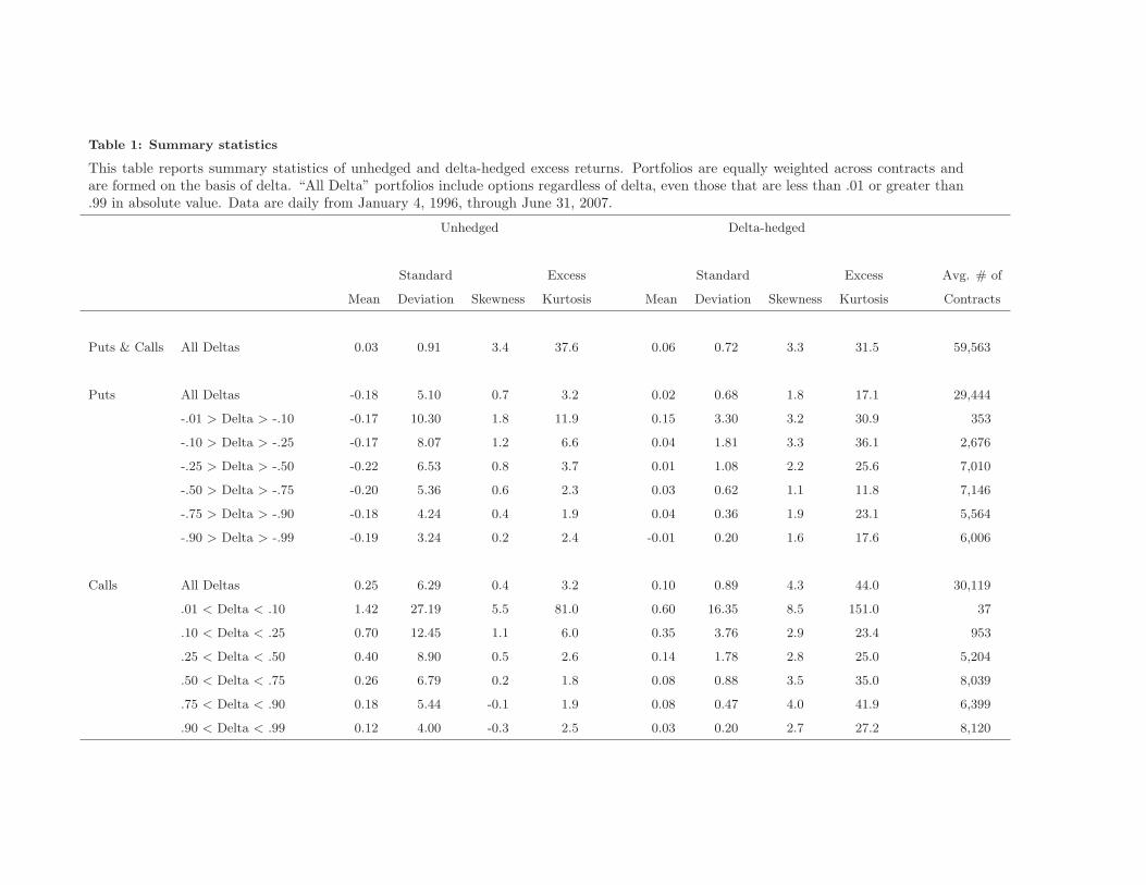
Table 1: Summary statistics

This table reports summary statistics of unhedged and delta-hedged excess returns. Portfolios are equally weighted across contracts andare formed on the basis of delta. “All Delta” portfolios include options regardless of delta, even those that are less than .01 or greater than.99 in absolute value. Data are daily from January 4, 1996, through June 31, 2007.

Unhedged Delta-hedged

Standard Excess Standard Excess Avg. # of

Mean Deviation Skewness Kurtosis Mean Deviation Skewness Kurtosis Contracts

Puts & Calls All Deltas 0.03 0.91 3.4 37.6 0.06 0.72 3.3 31.5 59,563

Puts All Deltas -0.18 5.10 0.7 3.2 0.02 0.68 1.8 17.1 29,444

-.01 > Delta > -.10 -0.17 10.30 1.8 11.9 0.15 3.30 3.2 30.9 353

-.10 > Delta > -.25 -0.17 8.07 1.2 6.6 0.04 1.81 3.3 36.1 2,676

-.25 > Delta > -.50 -0.22 6.53 0.8 3.7 0.01 1.08 2.2 25.6 7,010

-.50 > Delta > -.75 -0.20 5.36 0.6 2.3 0.03 0.62 1.1 11.8 7,146

-.75 > Delta > -.90 -0.18 4.24 0.4 1.9 0.04 0.36 1.9 23.1 5,564

-.90 > Delta > -.99 -0.19 3.24 0.2 2.4 -0.01 0.20 1.6 17.6 6,006

Calls All Deltas 0.25 6.29 0.4 3.2 0.10 0.89 4.3 44.0 30,119

.01 < Delta < .10 1.42 27.19 5.5 81.0 0.60 16.35 8.5 151.0 37

.10 < Delta < .25 0.70 12.45 1.1 6.0 0.35 3.76 2.9 23.4 953

.25 < Delta < .50 0.40 8.90 0.5 2.6 0.14 1.78 2.8 25.0 5,204

.50 < Delta < .75 0.26 6.79 0.2 1.8 0.08 0.88 3.5 35.0 8,039

.75 < Delta < .90 0.18 5.44 -0.1 1.9 0.08 0.47 4.0 41.9 6,399

.90 < Delta < .99 0.12 4.00 -0.3 2.5 0.03 0.20 2.7 27.2 8,120

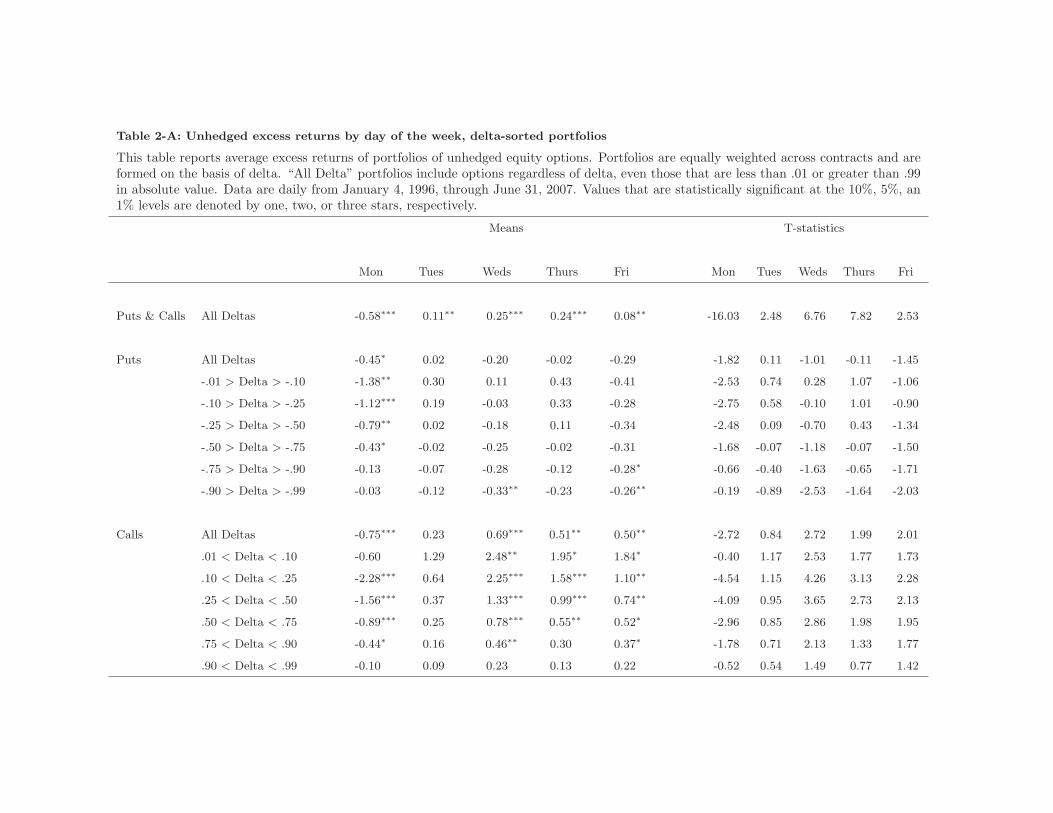
Table 2-A: Unhedged excess returns by day of the week, delta-sorted portfolios

This table reports average excess returns of portfolios of unhedged equity options. Portfolios are equally weighted across contracts and areformed on the basis of delta. “All Delta” portfolios include options regardless of delta, even those that are less than .01 or greater than .99in absolute value. Data are daily from January 4, 1996, through June 31, 2007. Values that are statistically significant at the 10%, 5%, an1% levels are denoted by one, two, or three stars, respectively.

Means T-statistics

Mon Tues Weds Thurs Fri Mon Tues Weds Thurs Fri

Puts & Calls All Deltas -0.58∗∗∗ 0.11∗∗ 0.25∗∗∗ 0.24∗∗∗ 0.08∗∗ -16.03 2.48 6.76 7.82 2.53

Puts All Deltas -0.45∗ 0.02 -0.20 -0.02 -0.29 -1.82 0.11 -1.01 -0.11 -1.45

-.01 > Delta > -.10 -1.38∗∗ 0.30 0.11 0.43 -0.41 -2.53 0.74 0.28 1.07 -1.06

-.10 > Delta > -.25 -1.12∗∗∗ 0.19 -0.03 0.33 -0.28 -2.75 0.58 -0.10 1.01 -0.90

-.25 > Delta > -.50 -0.79∗∗ 0.02 -0.18 0.11 -0.34 -2.48 0.09 -0.70 0.43 -1.34

-.50 > Delta > -.75 -0.43∗ -0.02 -0.25 -0.02 -0.31 -1.68 -0.07 -1.18 -0.07 -1.50

-.75 > Delta > -.90 -0.13 -0.07 -0.28 -0.12 -0.28∗ -0.66 -0.40 -1.63 -0.65 -1.71

-.90 > Delta > -.99 -0.03 -0.12 -0.33∗∗ -0.23 -0.26∗∗ -0.19 -0.89 -2.53 -1.64 -2.03

Calls All Deltas -0.75∗∗∗ 0.23 0.69∗∗∗ 0.51∗∗ 0.50∗∗ -2.72 0.84 2.72 1.99 2.01

.01 < Delta < .10 -0.60 1.29 2.48∗∗ 1.95∗ 1.84∗ -0.40 1.17 2.53 1.77 1.73

.10 < Delta < .25 -2.28∗∗∗ 0.64 2.25∗∗∗ 1.58∗∗∗ 1.10∗∗ -4.54 1.15 4.26 3.13 2.28

.25 < Delta < .50 -1.56∗∗∗ 0.37 1.33∗∗∗ 0.99∗∗∗ 0.74∗∗ -4.09 0.95 3.65 2.73 2.13

.50 < Delta < .75 -0.89∗∗∗ 0.25 0.78∗∗∗ 0.55∗∗ 0.52∗ -2.96 0.85 2.86 1.98 1.95

.75 < Delta < .90 -0.44∗ 0.16 0.46∗∗ 0.30 0.37∗ -1.78 0.71 2.13 1.33 1.77

.90 < Delta < .99 -0.10 0.09 0.23 0.13 0.22 -0.52 0.54 1.49 0.77 1.42

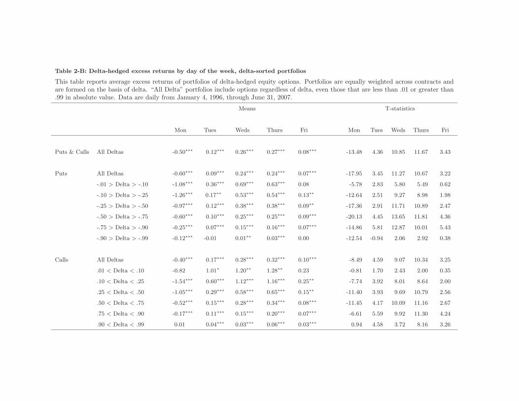
Table 2-B: Delta-hedged excess returns by day of the week, delta-sorted portfolios

This table reports average excess returns of portfolios of delta-hedged equity options. Portfolios are equally weighted across contracts andare formed on the basis of delta. “All Delta” portfolios include options regardless of delta, even those that are less than .01 or greater than.99 in absolute value. Data are daily from January 4, 1996, through June 31, 2007.

Means T-statistics

Mon Tues Weds Thurs Fri Mon Tues Weds Thurs Fri

Puts & Calls All Deltas -0.50∗∗∗ 0.12∗∗∗ 0.26∗∗∗ 0.27∗∗∗ 0.08∗∗∗ -13.48 4.36 10.85 11.67 3.43

Puts All Deltas -0.60∗∗∗ 0.09∗∗∗ 0.24∗∗∗ 0.24∗∗∗ 0.07∗∗∗ -17.95 3.45 11.27 10.67 3.22

-.01 > Delta > -.10 -1.08∗∗∗ 0.36∗∗∗ 0.69∗∗∗ 0.63∗∗∗ 0.08 -5.78 2.83 5.80 5.49 0.62

-.10 > Delta > -.25 -1.26∗∗∗ 0.17∗∗ 0.53∗∗∗ 0.54∗∗∗ 0.13∗∗ -12.64 2.51 9.27 8.98 1.98

-.25 > Delta > -.50 -0.97∗∗∗ 0.12∗∗∗ 0.38∗∗∗ 0.38∗∗∗ 0.09∗∗ -17.36 2.91 11.71 10.89 2.47

-.50 > Delta > -.75 -0.60∗∗∗ 0.10∗∗∗ 0.25∗∗∗ 0.25∗∗∗ 0.09∗∗∗ -20.13 4.45 13.65 11.81 4.36

-.75 > Delta > -.90 -0.25∗∗∗ 0.07∗∗∗ 0.15∗∗∗ 0.16∗∗∗ 0.07∗∗∗ -14.86 5.81 12.87 10.01 5.43

-.90 > Delta > -.99 -0.12∗∗∗ -0.01 0.01∗∗ 0.03∗∗∗ 0.00 -12.54 -0.94 2.06 2.92 0.38

Calls All Deltas -0.40∗∗∗ 0.17∗∗∗ 0.28∗∗∗ 0.32∗∗∗ 0.10∗∗∗ -8.49 4.59 9.07 10.34 3.25

.01 < Delta < .10 -0.82 1.01∗ 1.20∗∗ 1.28∗∗ 0.23 -0.81 1.70 2.43 2.00 0.35

.10 < Delta < .25 -1.54∗∗∗ 0.60∗∗∗ 1.12∗∗∗ 1.16∗∗∗ 0.25∗∗ -7.74 3.92 8.01 8.64 2.00

.25 < Delta < .50 -1.05∗∗∗ 0.29∗∗∗ 0.58∗∗∗ 0.65∗∗∗ 0.15∗∗ -11.40 3.93 9.69 10.79 2.56

.50 < Delta < .75 -0.52∗∗∗ 0.15∗∗∗ 0.28∗∗∗ 0.34∗∗∗ 0.08∗∗∗ -11.45 4.17 10.09 11.16 2.67

.75 < Delta < .90 -0.17∗∗∗ 0.11∗∗∗ 0.15∗∗∗ 0.20∗∗∗ 0.07∗∗∗ -6.61 5.59 9.92 11.30 4.24

.90 < Delta < .99 0.01 0.04∗∗∗ 0.03∗∗∗ 0.06∗∗∗ 0.03∗∗∗ 0.94 4.58 3.72 8.16 3.26

Table 3: Delta-hedged excess returns by day of the week, maturity-sorted portfolios

This table reports average excess returns of portfolios of delta-hedged equity options. Portfolios are equally weighted acrosscontracts and are formed on the basis of maturity. Data are daily from January 4, 1996, through June 31, 2007.

Means T-statistics

Mon Tues Weds Thurs Fri Mon Tues Weds Thurs Fri

Puts 1-10 days -1.16∗∗∗ 0.26∗∗∗ 0.45∗∗∗ 0.44∗∗∗ 0.05 -16.20 4.02 8.07 6.83 0.76

11-53 days -0.82∗∗∗ 0.09∗∗∗ 0.29∗∗∗ 0.28∗∗∗ 0.06∗∗ -19.31 2.73 11.13 10.86 2.11

54-118 days -0.41∗∗∗ 0.08∗∗∗ 0.20∗∗∗ 0.20∗∗∗ 0.10∗∗∗ -13.88 3.66 11.30 10.49 5.14

119-252 days -0.30∗∗∗ 0.06∗∗∗ 0.16∗∗∗ 0.16∗∗∗ 0.09∗∗∗ -12.11 3.40 10.10 9.54 5.21

253+ days 1.23 0.22 0.53∗ 0.02 0.23∗ 0.92 0.73 1.76 0.10 1.85

Calls 1-10 days -0.78∗∗∗ 0.46∗∗∗ 0.59∗∗∗ 0.58∗∗∗ 0.19∗ -8.22 5.03 6.53 7.54 1.95

11-53 days -0.60∗∗∗ 0.20∗∗∗ 0.36∗∗∗ 0.40∗∗∗ 0.10∗∗∗ -9.61 4.20 9.02 10.42 2.60

54-118 days -0.25∗∗∗ 0.13∗∗∗ 0.22∗∗∗ 0.27∗∗∗ 0.11∗∗∗ -5.84 4.26 8.95 10.05 4.32

119-252 days -0.16∗∗∗ 0.09∗∗∗ 0.16∗∗∗ 0.21∗∗∗ 0.11∗∗∗ -4.73 3.86 7.95 9.17 4.99

253+ days -0.28∗∗ 0.20 0.11 -0.76 0.11 -2.05 0.55 0.67 -1.11 1.13

39

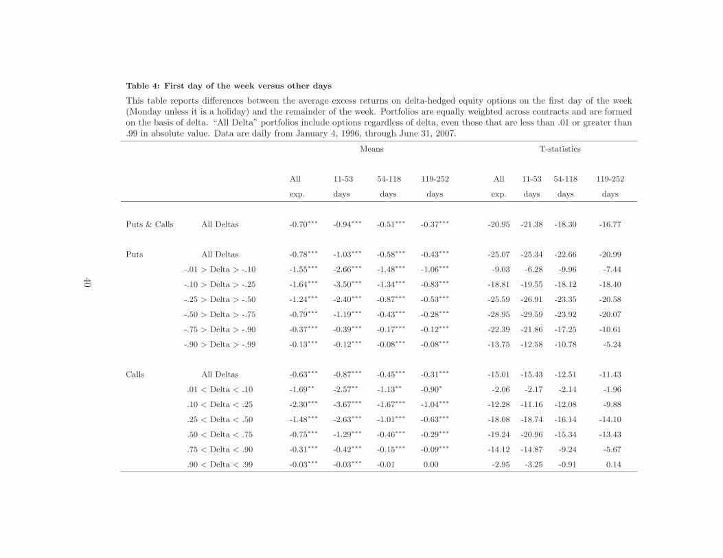
Table 4: First day of the week versus other days

This table reports differences between the average excess returns on delta-hedged equity options on the first day of the week(Monday unless it is a holiday) and the remainder of the week. Portfolios are equally weighted across contracts and are formedon the basis of delta. “All Delta” portfolios include options regardless of delta, even those that are less than .01 or greater than.99 in absolute value. Data are daily from January 4, 1996, through June 31, 2007.

Means T-statistics

All 11-53 54-118 119-252 All 11-53 54-118 119-252

exp. days days days exp. days days days

Puts & Calls All Deltas -0.70∗∗∗ -0.94∗∗∗ -0.51∗∗∗ -0.37∗∗∗ -20.95 -21.38 -18.30 -16.77

Puts All Deltas -0.78∗∗∗ -1.03∗∗∗ -0.58∗∗∗ -0.43∗∗∗ -25.07 -25.34 -22.66 -20.99

-.01 > Delta > -.10 -1.55∗∗∗ -2.66∗∗∗ -1.48∗∗∗ -1.06∗∗∗ -9.03 -6.28 -9.96 -7.44

-.10 > Delta > -.25 -1.64∗∗∗ -3.50∗∗∗ -1.34∗∗∗ -0.83∗∗∗ -18.81 -19.55 -18.12 -18.40

-.25 > Delta > -.50 -1.24∗∗∗ -2.40∗∗∗ -0.87∗∗∗ -0.53∗∗∗ -25.59 -26.91 -23.35 -20.58

-.50 > Delta > -.75 -0.79∗∗∗ -1.19∗∗∗ -0.43∗∗∗ -0.28∗∗∗ -28.95 -29.59 -23.92 -20.07

-.75 > Delta > -.90 -0.37∗∗∗ -0.39∗∗∗ -0.17∗∗∗ -0.12∗∗∗ -22.39 -21.86 -17.25 -10.61

-.90 > Delta > -.99 -0.13∗∗∗ -0.12∗∗∗ -0.08∗∗∗ -0.08∗∗∗ -13.75 -12.58 -10.78 -5.24

Calls All Deltas -0.63∗∗∗ -0.87∗∗∗ -0.45∗∗∗ -0.31∗∗∗ -15.01 -15.43 -12.51 -11.43

.01 < Delta < .10 -1.69∗∗ -2.57∗∗ -1.13∗∗ -0.90∗ -2.06 -2.17 -2.14 -1.96

.10 < Delta < .25 -2.30∗∗∗ -3.67∗∗∗ -1.67∗∗∗ -1.04∗∗∗ -12.28 -11.16 -12.08 -9.88

.25 < Delta < .50 -1.48∗∗∗ -2.63∗∗∗ -1.01∗∗∗ -0.63∗∗∗ -18.08 -18.74 -16.14 -14.10

.50 < Delta < .75 -0.75∗∗∗ -1.29∗∗∗ -0.46∗∗∗ -0.29∗∗∗ -19.24 -20.96 -15.34 -13.43

.75 < Delta < .90 -0.31∗∗∗ -0.42∗∗∗ -0.15∗∗∗ -0.09∗∗∗ -14.12 -14.87 -9.24 -5.67

.90 < Delta < .99 -0.03∗∗∗ -0.03∗∗∗ -0.01 0.00 -2.95 -3.25 -0.91 0.14

40

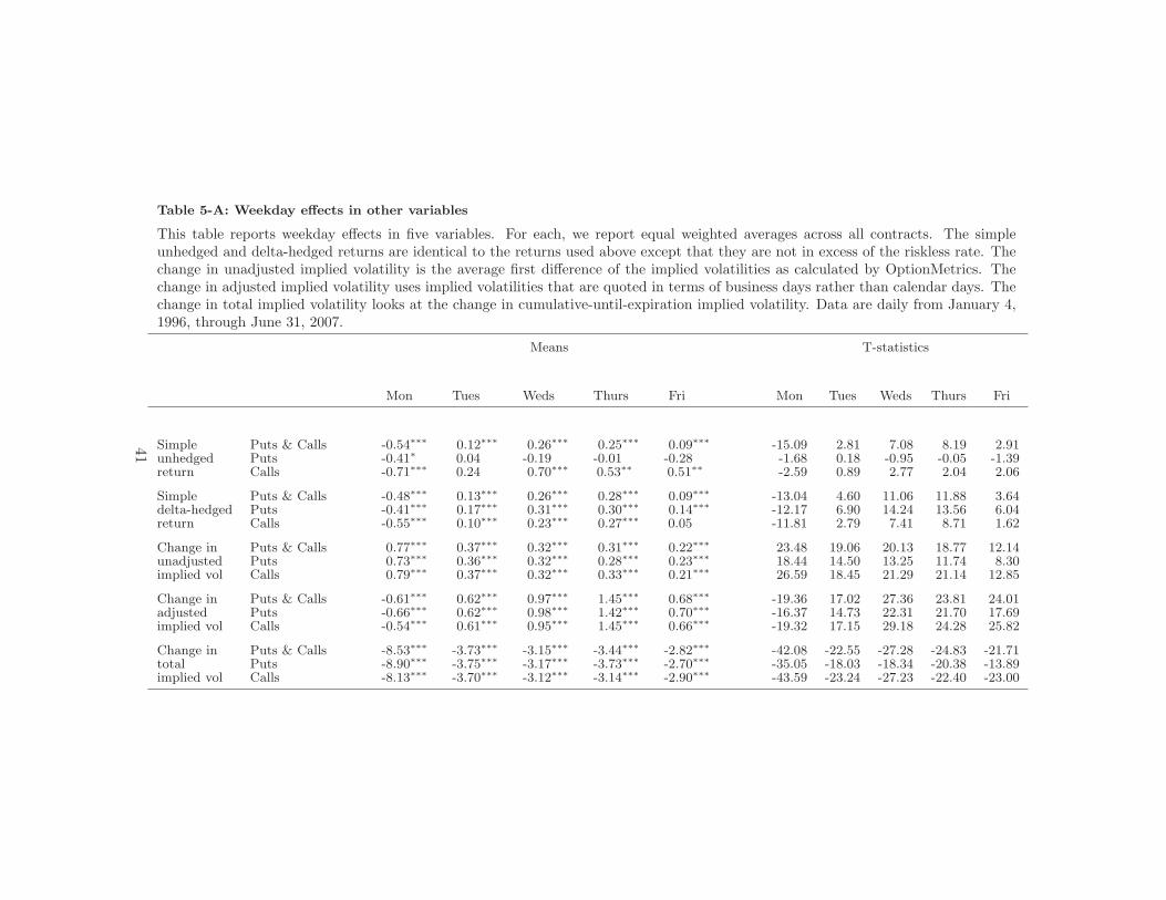
Table 5-A: Weekday effects in other variables

This table reports weekday effects in five variables. For each, we report equal weighted averages across all contracts. The simpleunhedged and delta-hedged returns are identical to the returns used above except that they are not in excess of the riskless rate. Thechange in unadjusted implied volatility is the average first difference of the implied volatilities as calculated by OptionMetrics. Thechange in adjusted implied volatility uses implied volatilities that are quoted in terms of business days rather than calendar days. Thechange in total implied volatility looks at the change in cumulative-until-expiration implied volatility. Data are daily from January 4,1996, through June 31, 2007.

Means T-statistics

Mon Tues Weds Thurs Fri Mon Tues Weds Thurs Fri

Simple Puts & Calls -0.54∗∗∗ 0.12∗∗∗ 0.26∗∗∗ 0.25∗∗∗ 0.09∗∗∗ -15.09 2.81 7.08 8.19 2.91unhedged Puts -0.41∗ 0.04 -0.19 -0.01 -0.28 -1.68 0.18 -0.95 -0.05 -1.39return Calls -0.71∗∗∗ 0.24 0.70∗∗∗ 0.53∗∗ 0.51∗∗ -2.59 0.89 2.77 2.04 2.06

Simple Puts & Calls -0.48∗∗∗ 0.13∗∗∗ 0.26∗∗∗ 0.28∗∗∗ 0.09∗∗∗ -13.04 4.60 11.06 11.88 3.64delta-hedged Puts -0.41∗∗∗ 0.17∗∗∗ 0.31∗∗∗ 0.30∗∗∗ 0.14∗∗∗ -12.17 6.90 14.24 13.56 6.04return Calls -0.55∗∗∗ 0.10∗∗∗ 0.23∗∗∗ 0.27∗∗∗ 0.05 -11.81 2.79 7.41 8.71 1.62

Change in Puts & Calls 0.77∗∗∗ 0.37∗∗∗ 0.32∗∗∗ 0.31∗∗∗ 0.22∗∗∗ 23.48 19.06 20.13 18.77 12.14unadjusted Puts 0.73∗∗∗ 0.36∗∗∗ 0.32∗∗∗ 0.28∗∗∗ 0.23∗∗∗ 18.44 14.50 13.25 11.74 8.30implied vol Calls 0.79∗∗∗ 0.37∗∗∗ 0.32∗∗∗ 0.33∗∗∗ 0.21∗∗∗ 26.59 18.45 21.29 21.14 12.85

Change in Puts & Calls -0.61∗∗∗ 0.62∗∗∗ 0.97∗∗∗ 1.45∗∗∗ 0.68∗∗∗ -19.36 17.02 27.36 23.81 24.01adjusted Puts -0.66∗∗∗ 0.62∗∗∗ 0.98∗∗∗ 1.42∗∗∗ 0.70∗∗∗ -16.37 14.73 22.31 21.70 17.69implied vol Calls -0.54∗∗∗ 0.61∗∗∗ 0.95∗∗∗ 1.45∗∗∗ 0.66∗∗∗ -19.32 17.15 29.18 24.28 25.82

Change in Puts & Calls -8.53∗∗∗ -3.73∗∗∗ -3.15∗∗∗ -3.44∗∗∗ -2.82∗∗∗ -42.08 -22.55 -27.28 -24.83 -21.71total Puts -8.90∗∗∗ -3.75∗∗∗ -3.17∗∗∗ -3.73∗∗∗ -2.70∗∗∗ -35.05 -18.03 -18.34 -20.38 -13.89implied vol Calls -8.13∗∗∗ -3.70∗∗∗ -3.12∗∗∗ -3.14∗∗∗ -2.90∗∗∗ -43.59 -23.24 -27.23 -22.40 -23.00

41

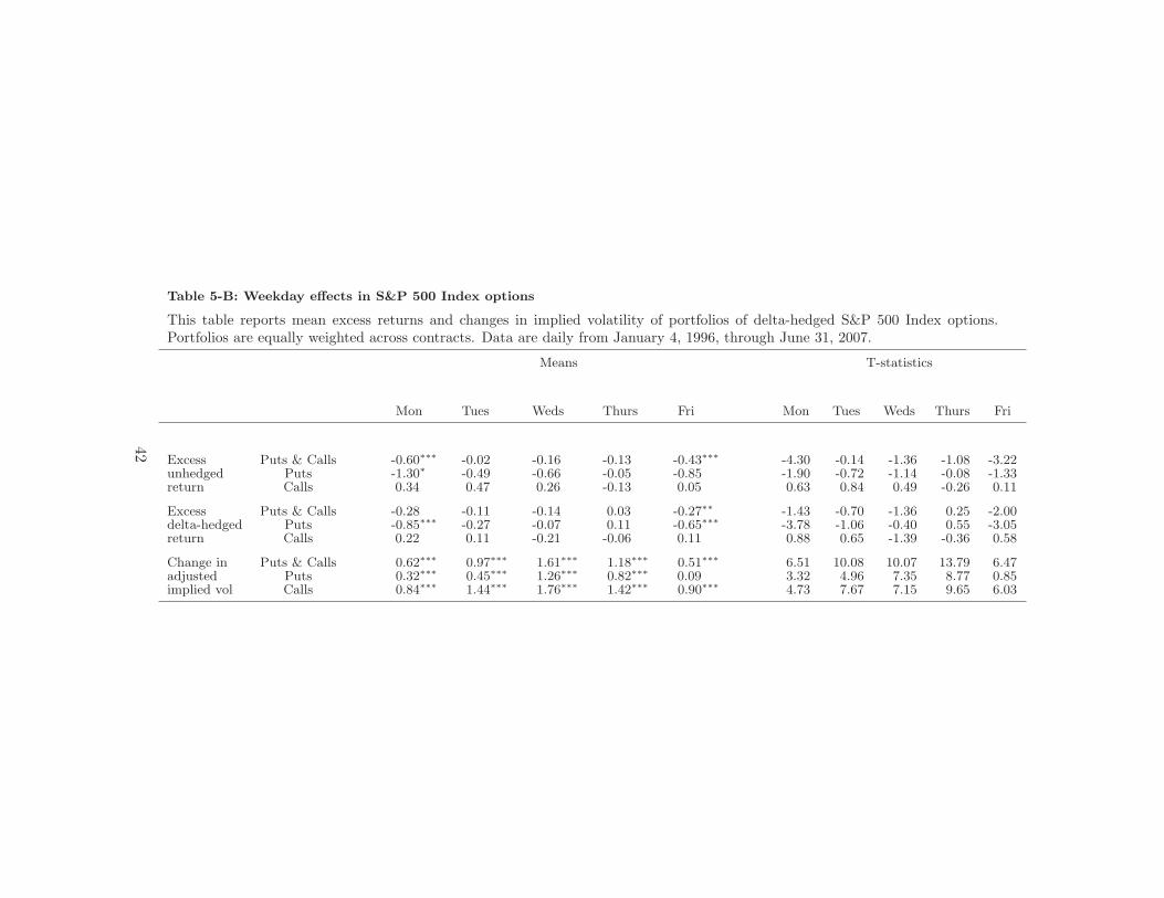
Table 5-B: Weekday effects in S&P 500 Index options

This table reports mean excess returns and changes in implied volatility of portfolios of delta-hedged S&P 500 Index options.Portfolios are equally weighted across contracts. Data are daily from January 4, 1996, through June 31, 2007.

Means T-statistics

Mon Tues Weds Thurs Fri Mon Tues Weds Thurs Fri

Excess Puts & Calls -0.60∗∗∗ -0.02 -0.16 -0.13 -0.43∗∗∗ -4.30 -0.14 -1.36 -1.08 -3.22unhedged Puts -1.30∗ -0.49 -0.66 -0.05 -0.85 -1.90 -0.72 -1.14 -0.08 -1.33return Calls 0.34 0.47 0.26 -0.13 0.05 0.63 0.84 0.49 -0.26 0.11

Excess Puts & Calls -0.28 -0.11 -0.14 0.03 -0.27∗∗ -1.43 -0.70 -1.36 0.25 -2.00delta-hedged Puts -0.85∗∗∗ -0.27 -0.07 0.11 -0.65∗∗∗ -3.78 -1.06 -0.40 0.55 -3.05return Calls 0.22 0.11 -0.21 -0.06 0.11 0.88 0.65 -1.39 -0.36 0.58

Change in Puts & Calls 0.62∗∗∗ 0.97∗∗∗ 1.61∗∗∗ 1.18∗∗∗ 0.51∗∗∗ 6.51 10.08 10.07 13.79 6.47adjusted Puts 0.32∗∗∗ 0.45∗∗∗ 1.26∗∗∗ 0.82∗∗∗ 0.09 3.32 4.96 7.35 8.77 0.85implied vol Calls 0.84∗∗∗ 1.44∗∗∗ 1.76∗∗∗ 1.42∗∗∗ 0.90∗∗∗ 4.73 7.67 7.15 9.65 6.03

42

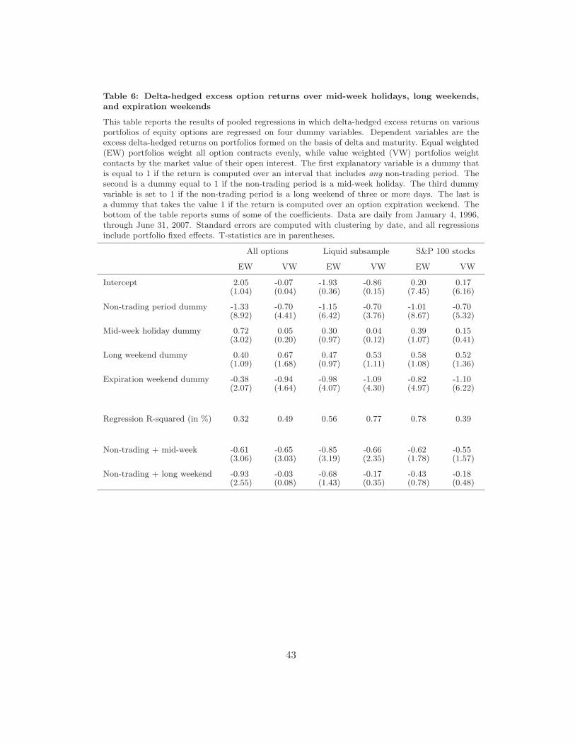
Table 6: Delta-hedged excess option returns over mid-week holidays, long weekends,

and expiration weekends

This table reports the results of pooled regressions in which delta-hedged excess returns on variousportfolios of equity options are regressed on four dummy variables. Dependent variables are theexcess delta-hedged returns on portfolios formed on the basis of delta and maturity. Equal weighted(EW) portfolios weight all option contracts evenly, while value weighted (VW) portfolios weightcontacts by the market value of their open interest. The first explanatory variable is a dummy thatis equal to 1 if the return is computed over an interval that includes any non-trading period. Thesecond is a dummy equal to 1 if the non-trading period is a mid-week holiday. The third dummyvariable is set to 1 if the non-trading period is a long weekend of three or more days. The last isa dummy that takes the value 1 if the return is computed over an option expiration weekend. Thebottom of the table reports sums of some of the coefficients. Data are daily from January 4, 1996,through June 31, 2007. Standard errors are computed with clustering by date, and all regressionsinclude portfolio fixed effects. T-statistics are in parentheses.

All options Liquid subsample S&P 100 stocks

EW VW EW VW EW VW

Intercept 2.05 -0.07 -1.93 -0.86 0.20 0.17(1.04) (0.04) (0.36) (0.15) (7.45) (6.16)

Non-trading period dummy -1.33 -0.70 -1.15 -0.70 -1.01 -0.70(8.92) (4.41) (6.42) (3.76) (8.67) (5.32)

Mid-week holiday dummy 0.72 0.05 0.30 0.04 0.39 0.15(3.02) (0.20) (0.97) (0.12) (1.07) (0.41)

Long weekend dummy 0.40 0.67 0.47 0.53 0.58 0.52(1.09) (1.68) (0.97) (1.11) (1.08) (1.36)

Expiration weekend dummy -0.38 -0.94 -0.98 -1.09 -0.82 -1.10(2.07) (4.64) (4.07) (4.30) (4.97) (6.22)

Regression R-squared (in %) 0.32 0.49 0.56 0.77 0.78 0.39

Non-trading + mid-week -0.61 -0.65 -0.85 -0.66 -0.62 -0.55(3.06) (3.03) (3.19) (2.35) (1.78) (1.57)

Non-trading + long weekend -0.93 -0.03 -0.68 -0.17 -0.43 -0.18(2.55) (0.08) (1.43) (0.35) (0.78) (0.48)

43

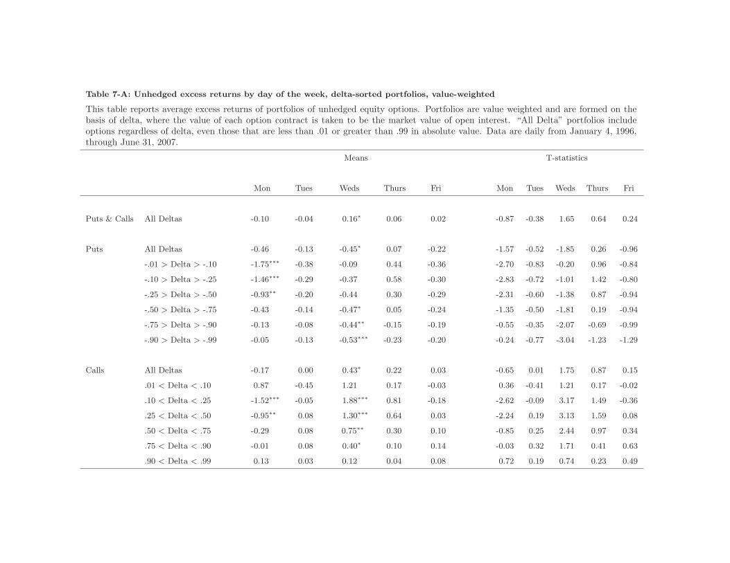
Table 7-A: Unhedged excess returns by day of the week, delta-sorted portfolios, value-weighted

This table reports average excess returns of portfolios of unhedged equity options. Portfolios are value weighted and are formed on thebasis of delta, where the value of each option contract is taken to be the market value of open interest. “All Delta” portfolios includeoptions regardless of delta, even those that are less than .01 or greater than .99 in absolute value. Data are daily from January 4, 1996,through June 31, 2007.

Means T-statistics

Mon Tues Weds Thurs Fri Mon Tues Weds Thurs Fri

Puts & Calls All Deltas -0.10 -0.04 0.16∗ 0.06 0.02 -0.87 -0.38 1.65 0.64 0.24

Puts All Deltas -0.46 -0.13 -0.45∗ 0.07 -0.22 -1.57 -0.52 -1.85 0.26 -0.96

-.01 > Delta > -.10 -1.75∗∗∗ -0.38 -0.09 0.44 -0.36 -2.70 -0.83 -0.20 0.96 -0.84

-.10 > Delta > -.25 -1.46∗∗∗ -0.29 -0.37 0.58 -0.30 -2.83 -0.72 -1.01 1.42 -0.80

-.25 > Delta > -.50 -0.93∗∗ -0.20 -0.44 0.30 -0.29 -2.31 -0.60 -1.38 0.87 -0.94

-.50 > Delta > -.75 -0.43 -0.14 -0.47∗ 0.05 -0.24 -1.35 -0.50 -1.81 0.19 -0.94

-.75 > Delta > -.90 -0.13 -0.08 -0.44∗∗ -0.15 -0.19 -0.55 -0.35 -2.07 -0.69 -0.99

-.90 > Delta > -.99 -0.05 -0.13 -0.53∗∗∗ -0.23 -0.20 -0.24 -0.77 -3.04 -1.23 -1.29

Calls All Deltas -0.17 0.00 0.43∗ 0.22 0.03 -0.65 0.01 1.75 0.87 0.15

.01 < Delta < .10 0.87 -0.45 1.21 0.17 -0.03 0.36 -0.41 1.21 0.17 -0.02

.10 < Delta < .25 -1.52∗∗∗ -0.05 1.88∗∗∗ 0.81 -0.18 -2.62 -0.09 3.17 1.49 -0.36

.25 < Delta < .50 -0.95∗∗ 0.08 1.30∗∗∗ 0.64 0.03 -2.24 0.19 3.13 1.59 0.08

.50 < Delta < .75 -0.29 0.08 0.75∗∗ 0.30 0.10 -0.85 0.25 2.44 0.97 0.34

.75 < Delta < .90 -0.01 0.08 0.40∗ 0.10 0.14 -0.03 0.32 1.71 0.41 0.63

.90 < Delta < .99 0.13 0.03 0.12 0.04 0.08 0.72 0.19 0.74 0.23 0.49

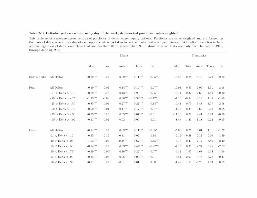
Table 7-B: Delta-hedged excess returns by day of the week, delta-sorted portfolios, value-weighted

This table reports average excess returns of portfolios of delta-hedged equity options. Portfolios are value weighted and are formed onthe basis of delta, where the value of each option contract is taken to be the market value of open interest. “All Delta” portfolios includeoptions regardless of delta, even those that are less than .01 or greater than .99 in absolute value. Data are daily from January 4, 1996,through June 31, 2007.

Means T-statistics

Mon Tues Weds Thurs Fri Mon Tues Weds Thurs Fri

Puts & Calls All Deltas -0.29∗∗∗ 0.01 0.09∗∗∗ 0.11∗∗∗ -0.05∗∗ -8.55 0.28 4.49 5.29 -2.39

Puts All Deltas -0.49∗∗∗ -0.02 0.14∗∗∗ 0.14∗∗∗ -0.07∗∗ -10.91 -0.53 5.09 4.31 -2.56

-.01 > Delta > -.10 -0.89∗∗∗ 0.06 0.43∗∗∗ 0.29∗ -0.05 -3.11 0.37 2.69 1.89 -0.32

-.10 > Delta > -.25 -1.13∗∗∗ -0.08 0.36∗∗∗ 0.39∗∗∗ -0.17∗ -7.26 -0.94 4.19 4.28 -1.89

-.25 > Delta > -.50 -0.85∗∗∗ -0.04 0.27∗∗∗ 0.27∗∗∗ -0.14∗∗∗ -10.41 -0.79 5.48 4.97 -2.98

-.50 > Delta > -.75 -0.50∗∗∗ -0.01 0.17∗∗∗ 0.17∗∗∗ -0.07∗∗∗ -11.77 -0.34 5.66 5.10 -2.68

-.75 > Delta > -.90 -0.23∗∗∗ 0.00 0.09∗∗∗ 0.07∗∗∗ -0.01 -11.10 0.21 4.41 3.23 -0.56

-.90 > Delta > -.99 -0.11∗∗∗ -0.02 -0.02 0.00 -0.01 -8.47 -1.49 -1.18 0.22 -0.55

Calls All Deltas -0.24∗∗∗ 0.02 0.09∗∗∗ 0.11∗∗∗ -0.05∗ -5.66 0.76 3.61 4.81 -1.77

.01 < Delta < .10 -0.25 -0.15 0.11 0.09 -1.14 -0.15 -0.28 0.23 0.16 -1.39

.10 < Delta < .25 -1.53∗∗∗ -0.07 0.38∗∗ 0.67∗∗∗ -0.45∗∗ -5.17 -0.40 2.17 3.80 -2.40

.25 < Delta < .50 -0.94∗∗∗ 0.03 0.33∗∗∗ 0.44∗∗∗ -0.22∗∗∗ -7.15 0.35 4.27 5.45 -2.72

.50 < Delta < .75 -0.39∗∗∗ 0.06∗ 0.16∗∗∗ 0.22∗∗∗ -0.07∗ -6.32 1.67 4.68 6.14 -1.96

.75 < Delta < .90 -0.15∗∗∗ 0.05∗∗∗ 0.06∗∗∗ 0.09∗∗∗ -0.01 -5.54 2.90 3.48 5.28 -0.41

.90 < Delta < .99 -0.01 0.01 -0.01 0.01 0.00 -1.49 1.51 -0.76 1.13 0.09

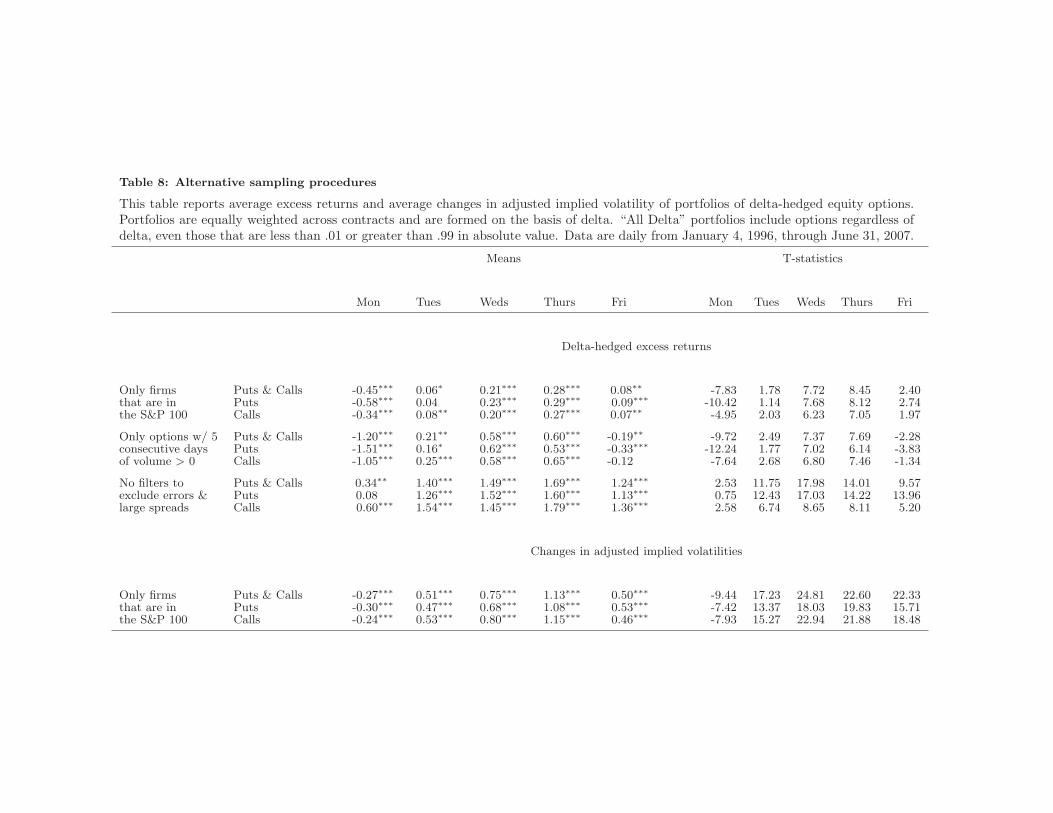
Table 8: Alternative sampling procedures

This table reports average excess returns and average changes in adjusted implied volatility of portfolios of delta-hedged equity options.Portfolios are equally weighted across contracts and are formed on the basis of delta. “All Delta” portfolios include options regardless ofdelta, even those that are less than .01 or greater than .99 in absolute value. Data are daily from January 4, 1996, through June 31, 2007.

Means T-statistics

Mon Tues Weds Thurs Fri Mon Tues Weds Thurs Fri

Delta-hedged excess returns

Only firms Puts & Calls -0.45∗∗∗ 0.06∗ 0.21∗∗∗ 0.28∗∗∗ 0.08∗∗ -7.83 1.78 7.72 8.45 2.40that are in Puts -0.58∗∗∗ 0.04 0.23∗∗∗ 0.29∗∗∗ 0.09∗∗∗ -10.42 1.14 7.68 8.12 2.74the S&P 100 Calls -0.34∗∗∗ 0.08∗∗ 0.20∗∗∗ 0.27∗∗∗ 0.07∗∗ -4.95 2.03 6.23 7.05 1.97

Only options w/ 5 Puts & Calls -1.20∗∗∗ 0.21∗∗ 0.58∗∗∗ 0.60∗∗∗ -0.19∗∗ -9.72 2.49 7.37 7.69 -2.28consecutive days Puts -1.51∗∗∗ 0.16∗ 0.62∗∗∗ 0.53∗∗∗ -0.33∗∗∗ -12.24 1.77 7.02 6.14 -3.83of volume > 0 Calls -1.05∗∗∗ 0.25∗∗∗ 0.58∗∗∗ 0.65∗∗∗ -0.12 -7.64 2.68 6.80 7.46 -1.34

No filters to Puts & Calls 0.34∗∗ 1.40∗∗∗ 1.49∗∗∗ 1.69∗∗∗ 1.24∗∗∗ 2.53 11.75 17.98 14.01 9.57exclude errors & Puts 0.08 1.26∗∗∗ 1.52∗∗∗ 1.60∗∗∗ 1.13∗∗∗ 0.75 12.43 17.03 14.22 13.96large spreads Calls 0.60∗∗∗ 1.54∗∗∗ 1.45∗∗∗ 1.79∗∗∗ 1.36∗∗∗ 2.58 6.74 8.65 8.11 5.20

Changes in adjusted implied volatilities

Only firms Puts & Calls -0.27∗∗∗ 0.51∗∗∗ 0.75∗∗∗ 1.13∗∗∗ 0.50∗∗∗ -9.44 17.23 24.81 22.60 22.33that are in Puts -0.30∗∗∗ 0.47∗∗∗ 0.68∗∗∗ 1.08∗∗∗ 0.53∗∗∗ -7.42 13.37 18.03 19.83 15.71the S&P 100 Calls -0.24∗∗∗ 0.53∗∗∗ 0.80∗∗∗ 1.15∗∗∗ 0.46∗∗∗ -7.93 15.27 22.94 21.88 18.48

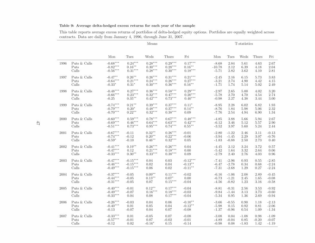
Table 9: Average delta-hedged excess returns for each year of the sample

This table reports average excess returns of portfolios of delta-hedged equity options. Portfolios are equally weighted acrosscontracts. Data are daily from January 4, 1996, through June 31, 2007.

Means T-statistics

Mon Tues Weds Thurs Fri Mon Tues Weds Thurs Fri

1996 Puts & Calls -0.68∗∗∗ 0.24∗∗∗ 0.28∗∗∗ 0.29∗∗∗ 0.17∗∗∗ -8.68 2.84 5.61 4.63 2.67Puts -0.82∗∗∗ 0.16∗∗ 0.30∗∗∗ 0.28∗∗∗ 0.16∗∗ -10.78 2.12 6.39 4.18 2.04Calls -0.56∗∗∗ 0.31∗∗∗ 0.28∗∗∗ 0.30∗∗∗ 0.18∗∗∗ -5.71 2.82 3.62 4.10 2.81

1997 Puts & Calls -0.47∗∗ 0.26∗∗ 0.26∗∗∗ 0.31∗∗∗ 0.21∗∗∗ -2.45 2.16 6.15 5.73 3.83Puts -0.64∗∗∗ 0.21∗∗∗ 0.24∗∗∗ 0.26∗∗∗ 0.27∗∗∗ -3.21 2.74 4.90 4.42 4.15Calls -0.33∗ 0.31∗ 0.30∗∗∗ 0.36∗∗∗ 0.16∗∗ -1.71 1.74 5.14 5.02 2.49

1998 Puts & Calls -0.48∗∗∗ 0.27∗∗∗ 0.36∗∗∗ 0.58∗∗∗ 0.29∗∗∗ -2.97 2.65 5.00 4.02 3.20Puts -0.66∗∗∗ 0.23∗∗∗ 0.32∗∗∗ 0.47∗∗∗ 0.20∗∗∗ -5.78 2.70 4.70 4.54 2.74Calls -0.25 0.35∗∗ 0.42∗∗∗ 0.73∗∗∗ 0.40∗∗∗ -0.98 2.27 4.38 3.44 3.00

1999 Puts & Calls -0.74∗∗∗ 0.21∗∗ 0.39∗∗∗ 0.37∗∗∗ 0.11∗ -8.95 2.28 6.02 6.82 1.93Puts -0.79∗∗∗ 0.20∗ 0.48∗∗∗ 0.37∗∗∗ 0.14∗∗ -8.76 1.84 5.98 5.06 2.32Calls -0.70∗∗∗ 0.22∗∗ 0.32∗∗∗ 0.38∗∗∗ 0.09 -7.76 2.54 4.94 6.90 1.34

2000 Puts & Calls -0.60∗∗∗ 0.59∗∗∗ 0.78∗∗∗ 0.67∗∗∗ 0.48∗∗∗ -4.85 3.88 5.66 5.94 2.67Puts -0.69∗∗∗ 0.46∗∗∗ 0.64∗∗∗ 0.63∗∗∗ 0.42∗∗∗ -6.12 3.46 5.12 5.57 2.90Calls -0.51∗∗∗ 0.73∗∗∗ 0.95∗∗∗ 0.74∗∗∗ 0.55∗∗ -3.52 3.97 5.60 5.24 2.44

2001 Puts & Calls -0.67∗∗∗ -0.11 0.32∗∗ 0.26∗∗∗ -0.01 -2.80 -1.22 2.46 3.11 -0.13Puts -0.74∗∗∗ -0.12 0.20∗∗ 0.22∗∗∗ -0.06 -3.94 -1.45 2.29 3.07 -0.76Calls -0.59∗ -0.10 0.46∗∗ 0.32∗∗∗ 0.05 -1.83 -0.88 2.50 2.73 0.40

2002 Puts & Calls -0.41∗∗∗ 0.19∗∗ 0.26∗∗∗ 0.26∗∗∗ 0.04 -4.45 2.12 3.24 3.72 0.57Puts -0.47∗∗∗ 0.12 0.21∗∗∗ 0.18∗∗∗ 0.00 -5.42 1.64 3.32 2.64 0.06Calls -0.33∗∗∗ 0.30∗∗ 0.33∗∗∗ 0.38∗∗∗ 0.09 -2.79 2.40 2.76 4.03 0.96

2003 Puts & Calls -0.47∗∗∗ -0.15∗∗∗ 0.04 0.03 -0.12∗∗∗ -7.41 -2.96 0.93 0.55 -2.85Puts -0.46∗∗∗ -0.15∗∗∗ 0.02 0.04 -0.13∗∗ -6.47 -2.78 0.34 0.68 -2.24Calls -0.49∗∗∗ -0.15∗∗∗ 0.06 0.02 -0.11∗∗ -7.31 -2.68 1.29 0.27 -2.24

2004 Puts & Calls -0.37∗∗∗ -0.05 0.09∗∗ 0.11∗∗∗ -0.02 -6.16 -1.06 2.08 2.89 -0.45Puts -0.44∗∗∗ -0.05 0.13∗∗ 0.07∗ 0.00 -6.73 -1.21 2.45 1.65 -0.08Calls -0.31∗∗∗ -0.05 0.07 0.15∗∗∗ -0.04 -4.56 -0.82 1.23 3.16 -0.58

2005 Puts & Calls -0.40∗∗∗ -0.01 0.12∗∗ 0.17∗∗∗ -0.04 -8.81 -0.31 2.56 3.53 -0.92Puts -0.49∗∗∗ -0.07 0.16∗∗∗ 0.18∗∗∗ -0.03 -9.84 -1.44 3.13 3.73 -0.60Calls -0.33∗∗∗ 0.04 0.08 0.17∗∗∗ -0.04 -5.34 0.95 1.36 2.69 -0.94

2006 Puts & Calls -0.26∗∗∗ -0.03 0.04 0.06 -0.10∗∗ -3.66 -0.55 0.90 1.18 -2.13Puts -0.40∗∗∗ 0.01 0.05 0.04 -0.12∗∗ -5.98 0.15 0.92 0.81 -2.06Calls -0.13 -0.07 0.04 0.07 -0.08 -1.37 -0.96 0.54 1.09 -1.34

2007 Puts & Calls -0.33∗∗∗ 0.01 -0.05 0.07 -0.08 -3.08 0.04 -1.08 0.98 -1.09Puts -0.57∗∗∗ -0.01 0.07 -0.02 -0.01 -4.89 -0.04 0.85 -0.20 -0.07Calls -0.12 0.02 -0.16∗ 0.15 -0.14 -0.98 0.08 -1.83 1.42 -1.19

47

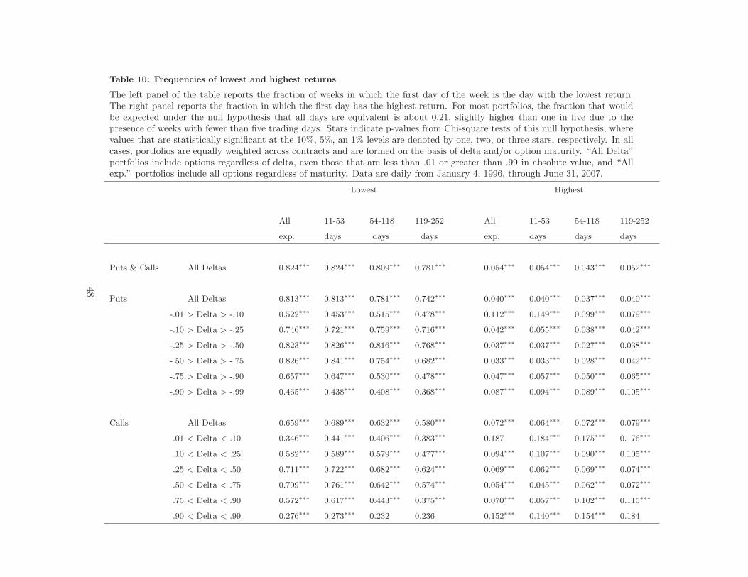
Table 10: Frequencies of lowest and highest returns

The left panel of the table reports the fraction of weeks in which the first day of the week is the day with the lowest return.The right panel reports the fraction in which the first day has the highest return. For most portfolios, the fraction that wouldbe expected under the null hypothesis that all days are equivalent is about 0.21, slightly higher than one in five due to thepresence of weeks with fewer than five trading days. Stars indicate p-values from Chi-square tests of this null hypothesis, wherevalues that are statistically significant at the 10%, 5%, an 1% levels are denoted by one, two, or three stars, respectively. In allcases, portfolios are equally weighted across contracts and are formed on the basis of delta and/or option maturity. “All Delta”portfolios include options regardless of delta, even those that are less than .01 or greater than .99 in absolute value, and “Allexp.” portfolios include all options regardless of maturity. Data are daily from January 4, 1996, through June 31, 2007.

Lowest Highest

All 11-53 54-118 119-252 All 11-53 54-118 119-252

exp. days days days exp. days days days

Puts & Calls All Deltas 0.824∗∗∗ 0.824∗∗∗ 0.809∗∗∗ 0.781∗∗∗ 0.054∗∗∗ 0.054∗∗∗ 0.043∗∗∗ 0.052∗∗∗

Puts All Deltas 0.813∗∗∗ 0.813∗∗∗ 0.781∗∗∗ 0.742∗∗∗ 0.040∗∗∗ 0.040∗∗∗ 0.037∗∗∗ 0.040∗∗∗

-.01 > Delta > -.10 0.522∗∗∗ 0.453∗∗∗ 0.515∗∗∗ 0.478∗∗∗ 0.112∗∗∗ 0.149∗∗∗ 0.099∗∗∗ 0.079∗∗∗

-.10 > Delta > -.25 0.746∗∗∗ 0.721∗∗∗ 0.759∗∗∗ 0.716∗∗∗ 0.042∗∗∗ 0.055∗∗∗ 0.038∗∗∗ 0.042∗∗∗

-.25 > Delta > -.50 0.823∗∗∗ 0.826∗∗∗ 0.816∗∗∗ 0.768∗∗∗ 0.037∗∗∗ 0.037∗∗∗ 0.027∗∗∗ 0.038∗∗∗

-.50 > Delta > -.75 0.826∗∗∗ 0.841∗∗∗ 0.754∗∗∗ 0.682∗∗∗ 0.033∗∗∗ 0.033∗∗∗ 0.028∗∗∗ 0.042∗∗∗

-.75 > Delta > -.90 0.657∗∗∗ 0.647∗∗∗ 0.530∗∗∗ 0.478∗∗∗ 0.047∗∗∗ 0.057∗∗∗ 0.050∗∗∗ 0.065∗∗∗

-.90 > Delta > -.99 0.465∗∗∗ 0.438∗∗∗ 0.408∗∗∗ 0.368∗∗∗ 0.087∗∗∗ 0.094∗∗∗ 0.089∗∗∗ 0.105∗∗∗

Calls All Deltas 0.659∗∗∗ 0.689∗∗∗ 0.632∗∗∗ 0.580∗∗∗ 0.072∗∗∗ 0.064∗∗∗ 0.072∗∗∗ 0.079∗∗∗

.01 < Delta < .10 0.346∗∗∗ 0.441∗∗∗ 0.406∗∗∗ 0.383∗∗∗ 0.187 0.184∗∗∗ 0.175∗∗∗ 0.176∗∗∗

.10 < Delta < .25 0.582∗∗∗ 0.589∗∗∗ 0.579∗∗∗ 0.477∗∗∗ 0.094∗∗∗ 0.107∗∗∗ 0.090∗∗∗ 0.105∗∗∗

.25 < Delta < .50 0.711∗∗∗ 0.722∗∗∗ 0.682∗∗∗ 0.624∗∗∗ 0.069∗∗∗ 0.062∗∗∗ 0.069∗∗∗ 0.074∗∗∗

.50 < Delta < .75 0.709∗∗∗ 0.761∗∗∗ 0.642∗∗∗ 0.574∗∗∗ 0.054∗∗∗ 0.045∗∗∗ 0.062∗∗∗ 0.072∗∗∗

.75 < Delta < .90 0.572∗∗∗ 0.617∗∗∗ 0.443∗∗∗ 0.375∗∗∗ 0.070∗∗∗ 0.057∗∗∗ 0.102∗∗∗ 0.115∗∗∗

.90 < Delta < .99 0.276∗∗∗ 0.273∗∗∗ 0.232 0.236 0.152∗∗∗ 0.140∗∗∗ 0.154∗∗∗ 0.184

48

Table 11: Relative bid-ask spreads, maturity-sorted portfolios

This table reports average bid-ask spreads, measured as a percentage of the bid-ask midpoint,of portfolios of equity options. All figures represent equally weighted averages across contracts.Data are daily from January 4, 1996, through June 31, 2007.

Means

Mon Tues Weds Thurs Fri

Puts All Deltas 8.9 8.9 8.9 8.9 8.8

-.01 > Delta > -.10 17.2 17.1 16.8 16.8 16.6

-.10 > Delta > -.25 14.6 14.6 14.4 14.3 14.2

-.25 > Delta > -.50 11.5 11.5 11.4 11.4 11.2

-.50 > Delta > -.75 8.9 8.9 8.9 9.0 8.8

-.75 > Delta > -.90 7.6 7.6 7.7 7.8 7.5

-.90 > Delta > -.99 4.9 4.9 5.0 5.1 4.8

Calls All Deltas 8.9 8.9 8.7 8.8 8.7

.01 < Delta < .10 23.7 23.8 22.8 22.2 22.1

.10 < Delta < .25 18.3 18.5 17.8 17.6 17.4

.25 < Delta < .50 13.6 13.6 13.3 13.3 13.1

.50 < Delta < .75 9.8 9.8 9.7 9.7 9.6

.75 < Delta < .90 7.8 7.8 7.8 7.9 7.7

.90 < Delta < .99 5.4 5.4 5.5 5.5 5.4

49

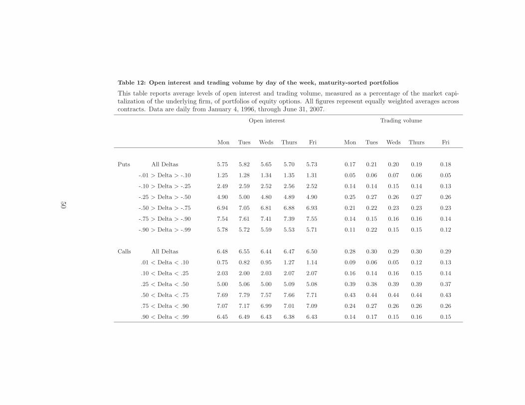
Table 12: Open interest and trading volume by day of the week, maturity-sorted portfolios

This table reports average levels of open interest and trading volume, measured as a percentage of the market capi-talization of the underlying firm, of portfolios of equity options. All figures represent equally weighted averages acrosscontracts. Data are daily from January 4, 1996, through June 31, 2007.

Open interest Trading volume

Mon Tues Weds Thurs Fri Mon Tues Weds Thurs Fri

Puts All Deltas 5.75 5.82 5.65 5.70 5.73 0.17 0.21 0.20 0.19 0.18

-.01 > Delta > -.10 1.25 1.28 1.34 1.35 1.31 0.05 0.06 0.07 0.06 0.05

-.10 > Delta > -.25 2.49 2.59 2.52 2.56 2.52 0.14 0.14 0.15 0.14 0.13

-.25 > Delta > -.50 4.90 5.00 4.80 4.89 4.90 0.25 0.27 0.26 0.27 0.26

-.50 > Delta > -.75 6.94 7.05 6.81 6.88 6.93 0.21 0.22 0.23 0.23 0.23

-.75 > Delta > -.90 7.54 7.61 7.41 7.39 7.55 0.14 0.15 0.16 0.16 0.14

-.90 > Delta > -.99 5.78 5.72 5.59 5.53 5.71 0.11 0.22 0.15 0.15 0.12

Calls All Deltas 6.48 6.55 6.44 6.47 6.50 0.28 0.30 0.29 0.30 0.29

.01 < Delta < .10 0.75 0.82 0.95 1.27 1.14 0.09 0.06 0.05 0.12 0.13

.10 < Delta < .25 2.03 2.00 2.03 2.07 2.07 0.16 0.14 0.16 0.15 0.14

.25 < Delta < .50 5.00 5.06 5.00 5.09 5.08 0.39 0.38 0.39 0.39 0.37

.50 < Delta < .75 7.69 7.79 7.57 7.66 7.71 0.43 0.44 0.44 0.44 0.43

.75 < Delta < .90 7.07 7.17 6.99 7.01 7.09 0.24 0.27 0.26 0.26 0.26

.90 < Delta < .99 6.45 6.49 6.43 6.38 6.43 0.14 0.17 0.15 0.16 0.15

50

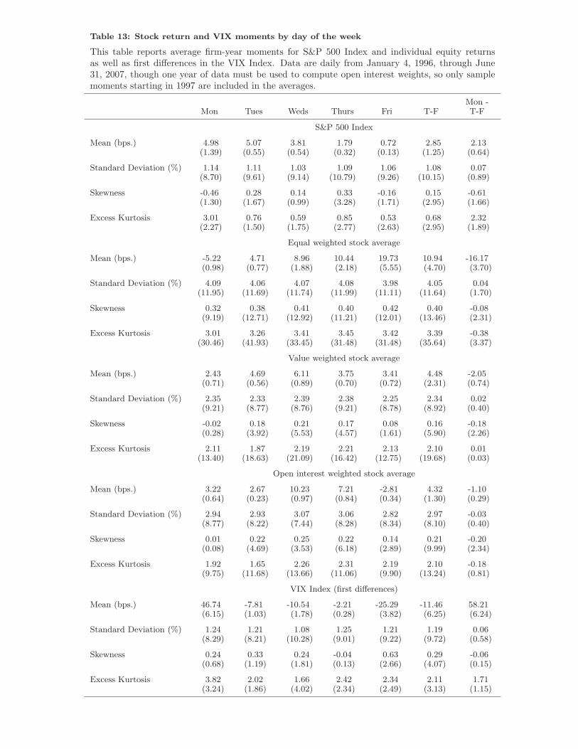
Table 13: Stock return and VIX moments by day of the week

This table reports average firm-year moments for S&P 500 Index and individual equity returnsas well as first differences in the VIX Index. Data are daily from January 4, 1996, through June31, 2007, though one year of data must be used to compute open interest weights, so only samplemoments starting in 1997 are included in the averages.

Mon -Mon Tues Weds Thurs Fri T-F T-F

S&P 500 Index

Mean (bps.) 4.98 5.07 3.81 1.79 0.72 2.85 2.13(1.39) (0.55) (0.54) (0.32) (0.13) (1.25) (0.64)

Standard Deviation (%) 1.14 1.11 1.03 1.09 1.06 1.08 0.07(8.70) (9.61) (9.14) (10.79) (9.26) (10.15) (0.89)

Skewness -0.46 0.28 0.14 0.33 -0.16 0.15 -0.61(1.30) (1.67) (0.99) (3.28) (1.71) (2.95) (1.66)

Excess Kurtosis 3.01 0.76 0.59 0.85 0.53 0.68 2.32(2.27) (1.50) (1.75) (2.77) (2.63) (2.95) (1.89)

Equal weighted stock average

Mean (bps.) -5.22 4.71 8.96 10.44 19.73 10.94 -16.17(0.98) (0.77) (1.88) (2.18) (5.55) (4.70) (3.70)

Standard Deviation (%) 4.09 4.06 4.07 4.08 3.98 4.05 0.04(11.95) (11.69) (11.74) (11.99) (11.11) (11.64) (1.70)

Skewness 0.32 0.38 0.41 0.40 0.42 0.40 -0.08(9.19) (12.71) (12.92) (11.21) (12.01) (13.46) (2.31)

Excess Kurtosis 3.01 3.26 3.41 3.45 3.42 3.39 -0.38(30.46) (41.93) (33.45) (31.48) (31.48) (35.64) (3.37)

Value weighted stock average

Mean (bps.) 2.43 4.69 6.11 3.75 3.41 4.48 -2.05(0.71) (0.56) (0.89) (0.70) (0.72) (2.31) (0.74)

Standard Deviation (%) 2.35 2.33 2.39 2.38 2.25 2.34 0.02(9.21) (8.77) (8.76) (9.21) (8.78) (8.92) (0.40)

Skewness -0.02 0.18 0.21 0.17 0.08 0.16 -0.18(0.28) (3.92) (5.53) (4.57) (1.61) (5.90) (2.26)

Excess Kurtosis 2.11 1.87 2.19 2.21 2.13 2.10 0.01(13.40) (18.63) (21.09) (16.42) (12.75) (19.68) (0.03)

Open interest weighted stock average

Mean (bps.) 3.22 2.67 10.23 7.21 -2.81 4.32 -1.10(0.64) (0.23) (0.97) (0.84) (0.34) (1.30) (0.29)

Standard Deviation (%) 2.94 2.93 3.07 3.06 2.82 2.97 -0.03(8.77) (8.22) (7.44) (8.28) (8.34) (8.10) (0.40)

Skewness 0.01 0.22 0.25 0.22 0.14 0.21 -0.20(0.08) (4.69) (3.53) (6.18) (2.89) (9.99) (2.34)

Excess Kurtosis 1.92 1.65 2.26 2.31 2.19 2.10 -0.18(9.75) (11.68) (13.66) (11.06) (9.90) (13.24) (0.81)

VIX Index (first differences)

Mean (bps.) 46.74 -7.81 -10.54 -2.21 -25.29 -11.46 58.21(6.15) (1.03) (1.78) (0.28) (3.82) (6.25) (6.24)

Standard Deviation (%) 1.24 1.21 1.08 1.25 1.21 1.19 0.06(8.29) (8.21) (10.28) (9.01) (9.22) (9.72) (0.58)

Skewness 0.24 0.33 0.24 -0.04 0.63 0.29 -0.06(0.68) (1.19) (1.81) (0.13) (2.66) (4.07) (0.15)

Excess Kurtosis 3.82 2.02 1.66 2.42 2.34 2.11 1.71(3.24) (1.86) (4.02) (2.34) (2.49) (3.13) (1.15)

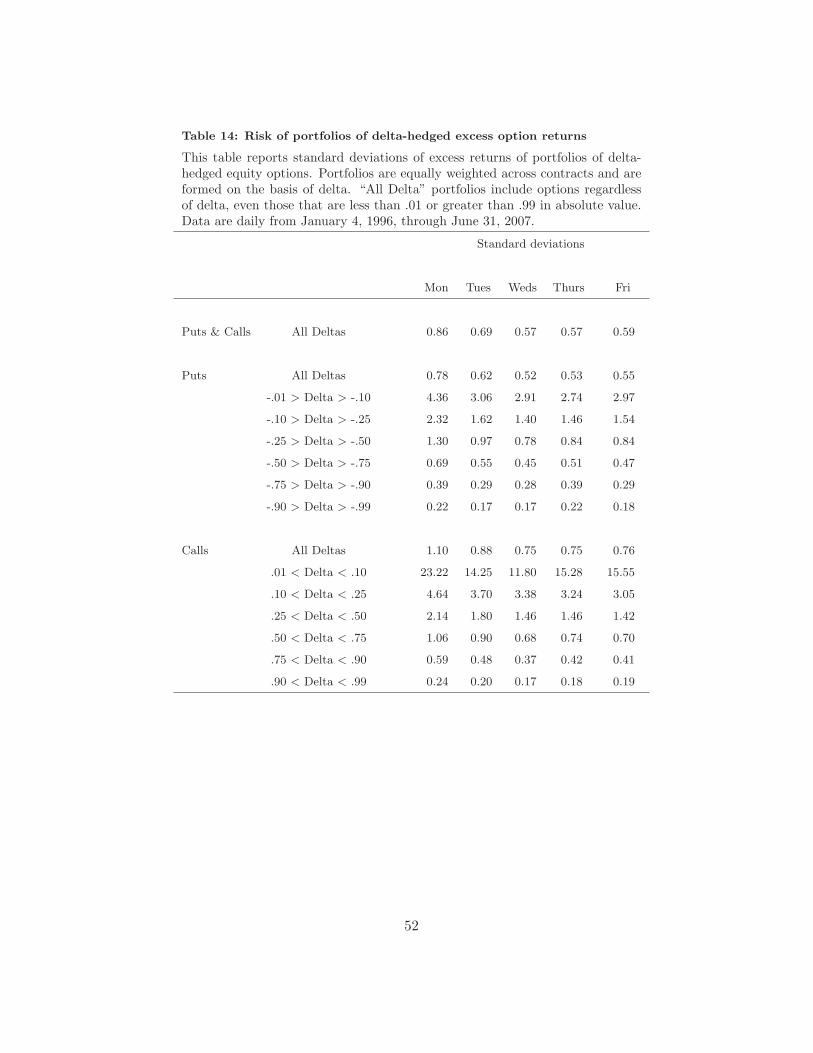
Table 14: Risk of portfolios of delta-hedged excess option returns

This table reports standard deviations of excess returns of portfolios of delta-hedged equity options. Portfolios are equally weighted across contracts and areformed on the basis of delta. “All Delta” portfolios include options regardlessof delta, even those that are less than .01 or greater than .99 in absolute value.Data are daily from January 4, 1996, through June 31, 2007.

Standard deviations

Mon Tues Weds Thurs Fri

Puts & Calls All Deltas 0.86 0.69 0.57 0.57 0.59

Puts All Deltas 0.78 0.62 0.52 0.53 0.55

-.01 > Delta > -.10 4.36 3.06 2.91 2.74 2.97

-.10 > Delta > -.25 2.32 1.62 1.40 1.46 1.54

-.25 > Delta > -.50 1.30 0.97 0.78 0.84 0.84

-.50 > Delta > -.75 0.69 0.55 0.45 0.51 0.47

-.75 > Delta > -.90 0.39 0.29 0.28 0.39 0.29

-.90 > Delta > -.99 0.22 0.17 0.17 0.22 0.18

Calls All Deltas 1.10 0.88 0.75 0.75 0.76

.01 < Delta < .10 23.22 14.25 11.80 15.28 15.55

.10 < Delta < .25 4.64 3.70 3.38 3.24 3.05

.25 < Delta < .50 2.14 1.80 1.46 1.46 1.42

.50 < Delta < .75 1.06 0.90 0.68 0.74 0.70

.75 < Delta < .90 0.59 0.48 0.37 0.42 0.41

.90 < Delta < .99 0.24 0.20 0.17 0.18 0.19

52

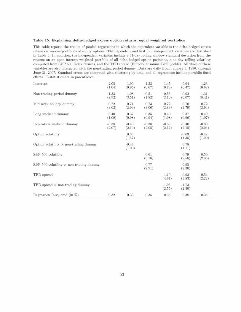
Table 15: Explaining delta-hedged excess option returns, equal weighted portfolios

This table reports the results of pooled regressions in which the dependent variable is the delta-hedged excessreturn on various portfolios of equity options. The dependent and first four independent variables are describedin Table 6. In addition, the independent variables include a 44-day rolling window standard deviation from thereturns on an open interest weighted portfolio of all delta-hedged option positions, a 44-day rolling volatilitycomputed from S&P 500 Index returns, and the TED spread (Eurodollar minus T-bill yields). All three of thesevariables are also interacted with the non-trading period dummy. Data are daily from January 4, 1996, throughJune 31, 2007. Standard errors are computed with clustering by date, and all regressions include portfolio fixedeffects. T-statistics are in parentheses.

Intercept 2.05 1.90 1.33 1.45 0.94 1.23(1.04) (0.95) (0.67) (0.73) (0.47) (0.62)

Non-trading period dummy -1.33 -1.08 -0.51 -0.55 -0.02 -1.31(8.92) (3.51) (1.82) (2.10) (0.07) (8.41)

Mid-week holiday dummy 0.72 0.71 0.73 0.72 0.70 0.72(3.02) (2.99) (3.06) (2.83) (2.79) (2.94)

Long weekend dummy 0.40 0.37 0.35 0.40 0.37 0.40(1.09) (0.98) (0.94) (1.08) (0.96) (1.07)

Expiration weekend dummy -0.38 -0.40 -0.38 -0.39 -0.40 -0.39(2.07) (2.10) (2.05) (2.12) (2.15) (2.04)

Option volatility 0.35 -0.63 -0.47(1.57) (1.35) (1.20)

Option volatility × non-trading dummy -0.44 0.78(1.00) (1.11)

S&P 500 volatility 0.61 0.79 0.59(3.78) (2.58) (2.35)

S&P 500 volatility × non-trading dummy -0.77 -0.95(2.91) (2.30)

TED spread 1.10 0.92 0.54(4.67) (3.83) (2.22)

TED spread × non-trading dummy -1.93 -1.73(2.55) (2.30)

Regression R-squared (in %) 0.32 0.33 0.35 0.35 0.38 0.35

53

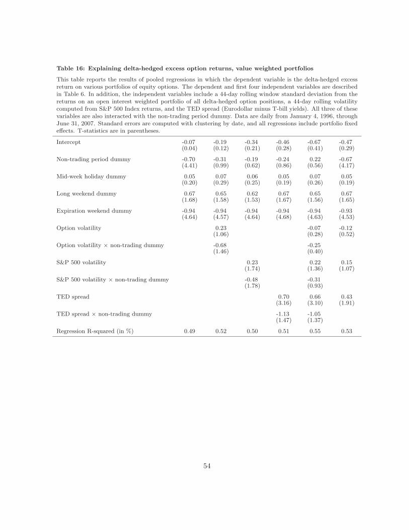
Table 16: Explaining delta-hedged excess option returns, value weighted portfolios

This table reports the results of pooled regressions in which the dependent variable is the delta-hedged excessreturn on various portfolios of equity options. The dependent and first four independent variables are describedin Table 6. In addition, the independent variables include a 44-day rolling window standard deviation from thereturns on an open interest weighted portfolio of all delta-hedged option positions, a 44-day rolling volatilitycomputed from S&P 500 Index returns, and the TED spread (Eurodollar minus T-bill yields). All three of thesevariables are also interacted with the non-trading period dummy. Data are daily from January 4, 1996, throughJune 31, 2007. Standard errors are computed with clustering by date, and all regressions include portfolio fixedeffects. T-statistics are in parentheses.

Intercept -0.07 -0.19 -0.34 -0.46 -0.67 -0.47(0.04) (0.12) (0.21) (0.28) (0.41) (0.29)

Non-trading period dummy -0.70 -0.31 -0.19 -0.24 0.22 -0.67(4.41) (0.99) (0.62) (0.86) (0.56) (4.17)

Mid-week holiday dummy 0.05 0.07 0.06 0.05 0.07 0.05(0.20) (0.29) (0.25) (0.19) (0.26) (0.19)

Long weekend dummy 0.67 0.65 0.62 0.67 0.65 0.67(1.68) (1.58) (1.53) (1.67) (1.56) (1.65)

Expiration weekend dummy -0.94 -0.94 -0.94 -0.94 -0.94 -0.93(4.64) (4.57) (4.64) (4.68) (4.63) (4.53)

Option volatility 0.23 -0.07 -0.12(1.06) (0.28) (0.52)

Option volatility × non-trading dummy -0.68 -0.25(1.46) (0.40)

S&P 500 volatility 0.23 0.22 0.15(1.74) (1.36) (1.07)

S&P 500 volatility × non-trading dummy -0.48 -0.31(1.78) (0.93)

TED spread 0.70 0.66 0.43(3.16) (3.10) (1.91)

TED spread × non-trading dummy -1.13 -1.05(1.47) (1.37)

Regression R-squared (in %) 0.49 0.52 0.50 0.51 0.55 0.53

54

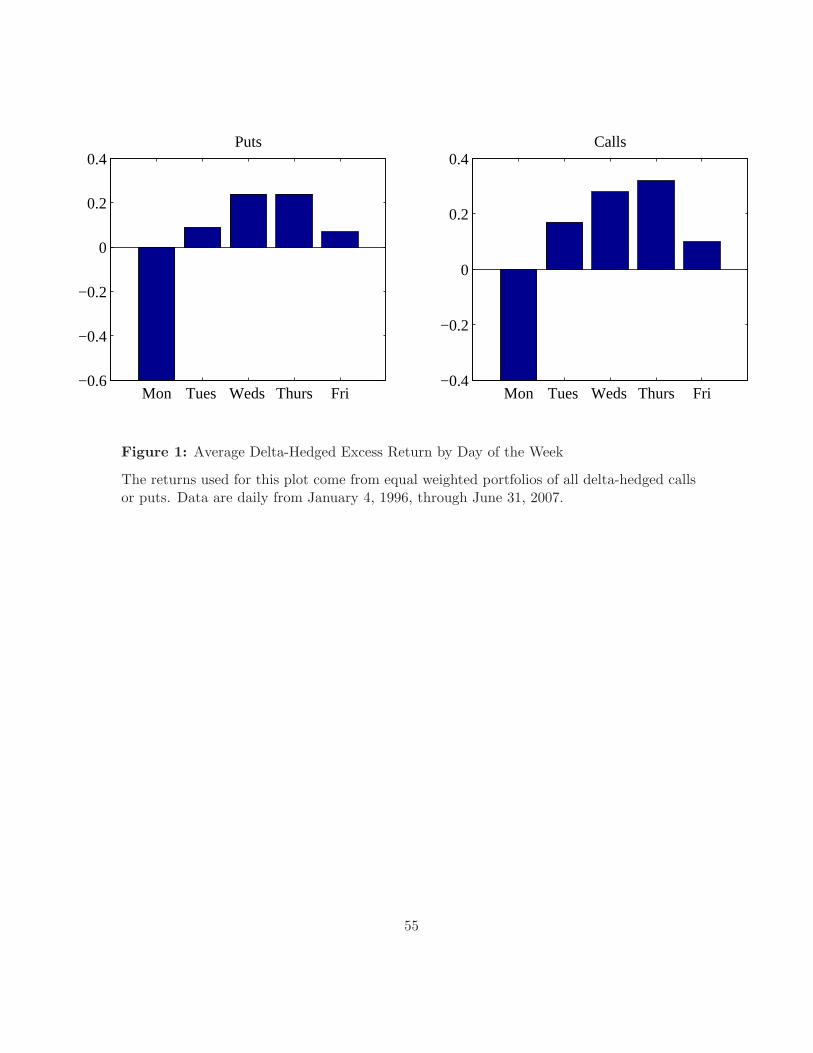
Mon Tues Weds Thurs Fri −0.6

−0.4

−0.2

0

0.2

0.4Puts

Mon Tues Weds Thurs Fri −0.4

−0.2

0

0.2

0.4Calls

Figure 1: Average Delta-Hedged Excess Return by Day of the Week

The returns used for this plot come from equal weighted portfolios of all delta-hedged callsor puts. Data are daily from January 4, 1996, through June 31, 2007.

55

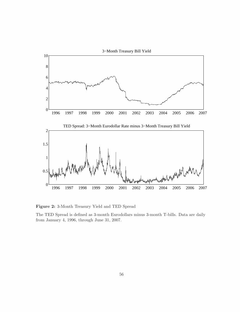
1996 1997 1998 1999 2000 2001 2002 2003 2004 2005 2006 20070

2

4

6

8

103−Month Treasury Bill Yield

1996 1997 1998 1999 2000 2001 2002 2003 2004 2005 2006 20070

0.5

1

1.5

2TED Spread: 3−Month Eurodollar Rate minus 3−Month Treasury Bill Yield

Figure 2: 3-Month Treasury Yield and TED Spread

The TED Spread is defined as 3-month Eurodollars minus 3-month T-bills. Data are dailyfrom January 4, 1996, through June 31, 2007.

56

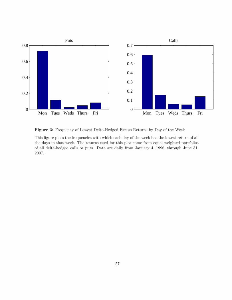
Mon Tues Weds Thurs Fri 0

0.2

0.4

0.6

0.8Puts

Mon Tues Weds Thurs Fri 0

0.1

0.2

0.3

0.4

0.5

0.6

0.7Calls

Figure 3: Frequency of Lowest Delta-Hedged Excess Returns by Day of the Week

This figure plots the frequencies with which each day of the week has the lowest return of allthe days in that week. The returns used for this plot come from equal weighted portfoliosof all delta-hedged calls or puts. Data are daily from January 4, 1996, through June 31,2007.

57