Project ReportATC-261

The Weather-Huffman Method of

Data Compression of Weather Images

J. Gertz

31 October 1997

Lincoln Laboratory MASSACHUSETTS INSTITUTE OF TECHNOLOGY

LEXINGTON, MASSACHUSETTS

Prepared for the Federal Aviation Administration, Washington, D.C. 20591

This document is available to the public through

the National Technical Information Service, Springfield, VA 22161

This document is disseminated under the sponsorship of the Department of Transportation in the interest of information exchange. The United States Government assumes no liability for its contents or use thereof.

1. Report No.

ATC-261

2. Government Accession No.

TECHNICAL REPORT STANDARD TITlE PAGE

3. Recipient's Catalog No.

4. Title and Subtitle

The Weather-Huffman Method of Data Compression ofWeather Images

7. Author(s)

Jeffrey L. Gertz

9. Performing Organization Name and Address

MIT Lincoln Laboratory244 Wood StreetLexington, MA 02173-9108

12. Sponsoring Agency Name and AddressDeparttnentofTr~po~tion

Federal Aviation AdministrationSystems Research and Development ServiceWashington, DC 20591

15. Supplementary Notes

5. Report Date31 October 1997

6. Performing Organization Code

8. Performing Organization Report No.

ATC-261

10. Work Unit No. (TRAIS)

11. Contract or Grant No.

DTFAO1-93-Z-Q2012

13. Type of Report and Period Covered

Project Report

14. Sponsoring Agency Code

This report is based on studies performed at Lincoln Laboratory, a center for research operated by Massachusetts Institute ofTechnology, under Air Force Contract FI9628-95-C-0002.

16. Abstract

Providing an accurate picture of the weather conditions in the pilot's area ofinterest is a highly useful application forground-ta-air datalinks. The problem with using data links to transmit weather graphics is the large number of bits requiredto exactly specify the weather image. To make transmission ofweather images practical, a means must be found to compressthe data to a size compatible with a limited datalink capacity.

The Weather-Huffman (WH) Algorithm developed in this report incorporates several subalgorithms in order toencode as faithfully as possible an input weather image within a specified datalink bit limitation. The main algorithmcomponent is the encodingofa version ofthe input image via the Weather Huffman runlength code, a variant ofthe standardHuffman code tailored to the peculiarities of weather images.

If possible, the input map itself is encoded. Generally, however, a resolution-reduced version of the map must becreated prior to the encoding to meet the bit limitation. In that case, the output map will contain blocky regions, and higherweather level areas will tend to bloom in size.

Two routines are included in WH to overcome these problems. The flI'St is a Smoother Process, which corrects theblocky edges of weather regions. The second, more powerful routine. is the Extra Bit Algorithm (EBA). EBA utilizes allbits remaining in the message after the Huffman encoding to correct pixels set at toohigh a weather leveL Both size and shapeof weather regions are adjusted by this algorithm.

Pictorial examples of the operation ofthis algorithm on several severe weather images derived from NEXRAD arepresented.

17. Key Words

Data CompressionWeather Images

18. Distribution Statement

This document is available to the public through theNational Technical Information Service,Springfield, VA 22161.

19. Security Classif. (of this report)

Unclassified

FORM DOT F 1700.7 (8-72)

20. Security Classif. (of this page)

Unclassified

Reproduction of completed page authorized

21. No. of Pages

88

22. Price

TABLE OF CONTENTS

List of IDustrations vList of Tables vi

l. INTRODUCTION 1

1.1 Weather Radar Infonnation 11.2 Ground-to-Air Data Links 11.3 Standard Compression Approaches 31.4 Weather Image Compression Algorithm 41.5 Report Outline 5

2. WEATIIER-HUFFMAN ALGORITHM OVERVIEW 7

2.1 Weather Image Huffman Code 72.2 Runlength Filtering and Resolution Reduction 102.3 Smoothing Process 102.4 Extra Bit Algorithm (EBA) 112.5 Sample Image Results 112.6 Program Size and Tuning Measures 14

3. HUFFMAN RUNLENGlH CODING 15

3.1 Image Scanning Procedures 153.2 Codeword Determination 183.3 Huffman Decoding Table Representation 20

4. WEATIIER-HUFFMAN CODING TABLE 25

4.1 Representation of Long Runlengths 254.2 Encoding "Other" Length Runs 254.3 Elimination of Long Codewords 274.4 Weather-Huffman (WH) Table Encoding 284.5 Encoding Codeword Lengths 304.6 Detennining the "Other" Length Breakpoint 314.7 Default Code Ensembles 32

5. WEATIffiR IMAGE SIMPLIFICATION 33

5.1 Runlength Filtering 335.2 Resolution Reduction 33

6. SMOOTIIING PROCESS 39

6.1 Smoothing Process Rules 396.2 Smoothing Process Implementation 396.3 Smoothing Process Operation 44

w

TABLE OF CONTENTS(continued)

7. THE EX1RA BIT ALGORI1HM (EBA)

7.1 Scoring of Quadrants for Extra Bit Application7.2 Selection of Classes for Extra Bit Application7.3 Encoding Algorithm for Extra Bit Application7.4 Decoding Algorithm for Extra Bit Application

8. WEATIffiR-HUFFMAN ALGORITHM ENCODING

8.1 Sequence of Encoding Methods8.2 Weather-Huffman Encoding Overview8.3 Building the Runlength Statistics8.4 Detennining the Codewords8.5 Encoding the Decoding Table8.6 Encoding the Image

9. WEATHER-HUFFMAN ALGORITHM DECODING

9.1 Decoder Control Logic9.2 Weather-Huffman (WH) Decoding Process9.3 Decoding Table Representation9.4 Decoding Table Creation9.5 Image Runlength Decoding

10. WEATHER-HUFFMAN ALGORITHM RESULTS

10.1 Degrees ofResolution Reduction10.2 Incremental Results10.2 Algorithm Tradeoffs10.3 Variation in Link Bit Limit

APPENDIX A

APPENDIXB

REFERENCES

IV

45

45464748

51

515354555757

59

5960616163

65

65656666

73

77

79

FigureNo.

1-1

1-2

1-32-1

2-2a

2-2b

3-1

3-2

3-3

3-4

5-1

5-2

5-3

6-1

6-2

6-3

6-4

8-1

8-2

8-3

10-1

10-2

LIST OF ILLUSTRATIONS

Sample stormy weather image.

Sample weather regions showing the "contiguity" of weather images.

Sample weather region showing weather transition levels.

The Hilbert Scan for a 32*32 square. Each quadrant (different line type)

is completed before another is entered.

Compression performance at 3500 bits.

Compression performance at 3500 bits.

The Hilbert scan for a 32*32 square. Each quadrant (different line type)

is completed before another is entered.

The Hilbert scan of a typical weather region. Several long meanderingruns and several short "nick" runs are produced.

List generation procedure for an ensemble of six runlengths and theirassociated probabilities.

A complete binary tree specifying the Huffman codewords.

Effect of filtering weather images.

Superpixel settings generated from the indicated level 2 counts.

Mobile image encoded at various levels of resolution reduction.

Rules of smoothing process algorithm.

Examples of application of smoothing process rules.

Example of smoothing process algorithm applied to sample weatherregion.

Effect of various levels of smoothing on output New York image.

An example of Weather-Huffman resolution reduction (numbers areweather levels).

Example case indicating extension of S2 run.

Example where 0 length run specification is not required.

Effect of different resolution reduction levels on New York image. Asresolution decreases, image fidelity degrades but bit requirement drops.

Effect of runlength fIltering of lower resolution levels on New Yorkimage. Fidelity undergoes minor change while bit requirement dropssignificantly.

v

Page

2

4

5

8

12

13

16

17

19

20

34

36

37

40

41

42

43

52

54

58

67

68

FigureNo.

LIST OF ILLUSTRATIONS(continued)

Page

10-3 Output New York image existing after each incremental step of theWH algorithm. 69

104 Tradeoff for Allison image between resolution and extra bits. Extra bitalgorithm compensates for resolution reduction by using bits freed up byapplication of lower resolution. 70

10-5a Output Mobile image as a function of datalink bit limit 71

1O-5b Output Allison image as a function of datalink: bit limit 72

LIST OF TABLES

TableNo.

1 National Weather Service Reflectivity Levels

vi

Page

3

1. INTRODUCTION

It is often said that "a picture is worth a thousand words". This is certainly the case when itcomes to giving the pilot of an aircraft a description of the weather. Providing an accurate pictureof the weather conditions in the pilot's area of interest could be a highly useful application of aground-ta-air datalink. Even those pilots that have onboard weather radars could profit from theability to see the weather in regions beyond the range of their radar, or seeing the nearby regionwith the greater clarity that a ground-based weather radar can provide.

1.1 WEATHER RADAR INFORMATION

The present TDWR (Tenninal Doppler Weather Radar), ASR-9 (Airport SurveillanceRadar), and NEXRAD (NEXt generation weather RADar) radars are designed to providehazardous weather information to controllers located at the tower or at an enroute center. While thevoice message pilots receive from the terminal controllers will facilitate the avoidance of hazardousweather, it will not provide "escape" infonnation. The lack of vectoring instructions will leave thechoice of alternate flight paths to the pilot. With such a system, the possibility of a pilotencountering weather situations as dangerous, or even more dangerous, than those in the verbalwarning, or his not understanding the message enough to avoid the hazard, becomes a possiblescenario.

During the enroute portions of flight, graphical weather infonnation could be used in anumber of applications to increase flight safety. This infonnation would be useful as warnings ofimmediate weather hazards that need be avoided, as infonnation of possible escape maneuversonce hazardous weather has been encountered, and for long range strategic flight path planninginfonnation. Because NEXRAD images are so important to in-flight decision making, they areused as examples throughout this report.

1.2 GROUND·TO·AIR DATA LINKS

To provide pilots with the infonnation needed to make informed decisions on the avoidanceof hazardous weather, and to supply them with the same infonnation the controllers have, the FAAis actively developing the capability to provide real time graphical information of hazardousweather conditions to aircraft by use of datalink. Several fonns of ground-to-air datalinks arecurrently under development.

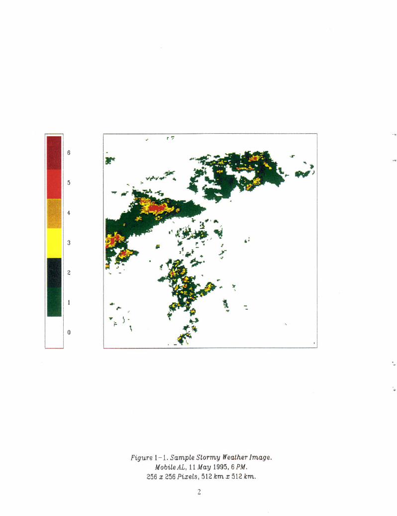
The problem with using any datalink: to transmit weather graphics is the large number ofbits required to specify a weather image. For the purposes of this report, a weather image isdefined as an array of 256x256 (65,536) pixels. This array size is typical of a graphic, such as aNEXRAD image, that could be transmitted and displayed in an aircraft using modem equipment.Each pixel can indicate either clear sky or one of the six National Weather Service weatherreflectivity levels (see Table 1 below), and thus requires 3 bits to specify. Hence, a weatherimage, such as the example shown in Figure 1-1, will consist of 196,608 bits of infonnation, notcounting any datalink overhead. This size will impose a severe load upon any practical ground-to­air datalink.

1

r r;

6

r ·r

.~

5.....""*.J9# . ...

4-

3

2

~ !r'... 1-{"-

~

... ~I -;:.0 \

Figure 1-1. Sample Stormy Weather Image.

MobileAL, 11 May 1995, 6 PM.256 x 256 Pixels, 512 km x 512 km.

2

Table 1. National Weather Service Reflectivity Levels

NWSLevel

Precip.Intensity

Rainfallinlhr

PossibleTurbulence Hail Lightning

LEVEL 6 Extreme ;:: 7.1 Severe Large Yes

LEVEL 5 Intense 4.5-7.1 Severe Likely Yes

LEVEL 4 Very Strong 2.2-4.5 Severe - Yes

LEVEL 3 Strong 1.1-2.2 Severe - Yes

LEVEL 2 Moderate 0.2-1.1 Light! - NoModerate

LEVEL 1 Weak < 0.2 Light! - NoModerate

To make transmission of weather images using datalinks practical, a means must be foundto significantly compress the image; a typical aeronautical datalink would require a 65-to-1compression if it were to limit the uplinked image transmission to 3600 bits. In addition, thealgorithms used to perform the compression and decompression must be computationally efficient:the ground computer may have to handle many aircraft requests in a given scan, and the airbornecomputer may not be particularly powerful or have extensive memory capacity.

1.3 STANDARD COMPRESSION APPROACHES

There are many data compression techniques that are well-developed and documented.These techniques include runlength encoding, select encoding, Huffman encoding, Lempel-Zivencoding, and arithmetic encoding [1]. These algorithms are drawn from a variety of applicationsincluding text-file archiving, compression of Fax images, and transmission of general pictures. Allof these approaches make use of the redundancies in the data to achieve compression. They aregeneral techniques, independent of the nature of the data. They also maintain exact fidelity undercompression - the decompressed image exactly matches the raw image. However, as a result ofthis property, they cannot guarantee a maximum bit limit

Several of these general approaches were tested on sample weather images taken fromoperating weather radars as well as from weather service providers [2]. The best of theseapproaches, the Huffman [3], could only produce compressions of the order of 3-t0-1 or 4-to-l onthe sample images. None ever achieved the compressions required to fit weather images intotypical datalink limitations. It became clear that an algorithm based on the unique attributes ofweather images would be required to achieve the necessary compression.

It also became apparent that exact fidelity under compression could not always be achievedfor this application; some amount of distortion in the transmission of the weather images over thedatalink would often have to be tolerated. This opened the door to modem data compressionapproaches such as fractals, cosine transforms, and wavelets. These algorithms were found to beinappropriate for the types of graphics represented by weather images (few bits, low redundancy),and also require too great an encoding and decoding overhead for the target class of computers,especially those aboard general aviation aircraft

3

As a result of these observations, two methods of compression tailored to weather imageswere developed at lincoln Laboratory: Polygon-Ellipse [4] and Weather-Huffman. Polygon­Ellipse was implemented and field tested first, but human factors evaluation indicated that theimages produced were unacceptable at high compression levels. Later evaluations indicated thatWeather-Huffman removed the drawbacks noted by subject pilots.

The algorithm described in the remainder of this report, specially tailored for weatherimages, maximizes the number of images that can be sent exactly. When lossless representation isimpossible, it trades off controlled amounts of distortion for increased compression. The ultimatetest of this algorithm is that it produces useful and accurate images when bit-limited byrepresentative ground-to-air datalink limits.

1.4 WEATHER IMAGE COMPRESSION ALGORITHM

Weather images exhibit a great deal of structure - they are far from random sets of pixels.If the compression algorithm can make use of this structure, the result will be the achievement ofgreater compression than would be possible for a "general" algorithm which simply depended onthe basic redundancy of the image.

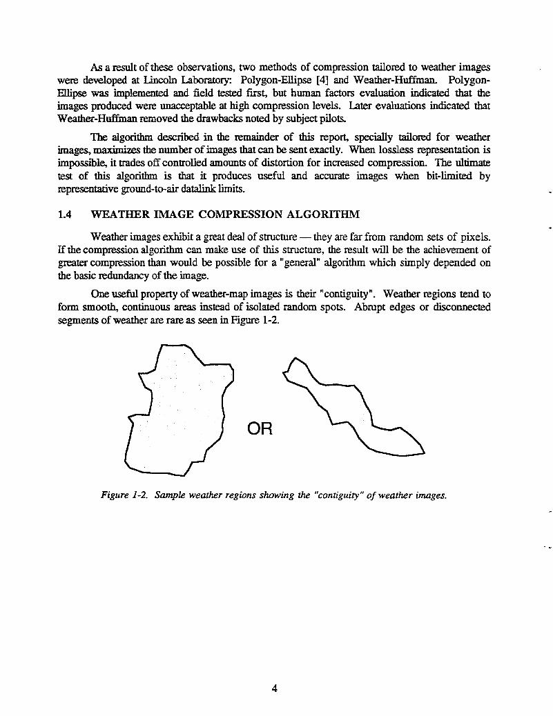
One useful property of weather-map images is their "contiguity". Weather regions tend toform smooth, continuous areas instead of isolated random spots. Abrupt edges or disconnectedsegments of weather are rare as seen in Figure 1-2.

OR

Figure 1-2. Sample weather regions showing the "contiguity" o/weather images.

4

A second property of weather images might be termed "continuity" - regions of intense(higher-level) weather usually are wholly contained within regions of less intense weather. In fact,weather transitions are generally restricted to plus or minus one level as seen in Figure 1-3.

Figure 1-3. Sample weather region showing weather transition levels.

These two properties are exploited in the compression technique developed in this projectThe Weather-Huffman (WH) Algorithm. The key element of the WH algorithm is a Huffman-typerunlength encoding scheme that has built-in assumptions tied to typical weather images; when theseassumptions hold, the bit requirements of WH are far less than the theoretically optimum Huffmancode.

The WH algorithm contains procedures for gracefully degrading the resolution of thetransmitted image when necessary to meet a specified bit limit. It also contains an auxiliary ExtraBit Algorithm (EBA) which makes use of any bits remaining after the WH compression step torestore as much as possible of the fidelity lost by this resolution reduction.

1.S REPORT OUTLINE

Section 2 of this report provides an overview of the Weather-Huffman (WH) approach toweather image compression. This section also includes results of applying the algorithm with a bitlimitation (3500 bits) to sample complex real-life weather images. Finally, it estimates the groundcomputer and onboard avionics requirements for implementing the WH encoding and decodingroutines.

Section 3 provides an overview of the theory of the Huffman runlength algorithm, thefoundation of the WH approach. It also presents the principles of the decoding table, which must

5

be included with the encoded image in the uplink message in order to permit the decoder todecipher the sequence of codewords that constitute the image representation.

Section 4 then details the complex procedures used to convert the general Huffman methodto one that applies specifically to the weather image situation. In particular, the techniquesemployed to compress the bit requirements of the decoding table are described in depth. Withoutthese modifications, the decoding table alone could use up all the bits of the uplink message.

Section 5 then presents the methods needed to simplify the input weather image when itsexact representation exceeds the datalink bit limit. Both mtering and resolution reduction of theweather image are employed. The fonner eliminates isolated pixels to reduce the number of runson the image, while the latter maps a block of pixels into a single "superpixel" (2x2->1, or 4x4->I ,or 8x8->1) to reduce the number of pixels to encode.

Section 6 then presents the smoothing algorithm employed by the decoder to eliminate theblockiness of the decoded image that results whenever resolution reduction was required. That is,the edges of a 2x2, 4x4, or 8x8 expansion are modified to better match the true shapes of weatherregions.

Section 7 provides the details of the Extra Bit Algorithm (EBA), which utilizes all messagebits remaining after the Huffman encoding of the image to improve the accuracy of the decodedimage whenever resolution reduction was required. In particular, it specifies which quadrants of a1->2x2 expansion should be set to a weather level other than the level of the expanded superpixeL

Finally, Sections 8 and 9 present the complete set of steps used by the encoder and decoderrespectively in the Weather-Huffman Algorithm, making use of the information provided in theearlier sections. They also provides a detailed description of the bit format of the encoded datastream sent on the datalink. The level of detail provided in these sections is sufficient for aprogrammer to understand the C-coded subroutines developed as part of this project.

Sample results of the Weather-Huffman algorithm are presented in Section 10. The effectsof including or omitting each part of the algorithm are illustrated, so that the relevant tradeoffs canbe realized. Also various bit limitations are explored, so that the graceful degradation of theapproach will be apparent

Appendix A presents, for each weather level, the three default codeword sets available forthe Huffman encoding step. Appendix B lists the set of user-specified parameters that currentlyexist in the WH software. For each, an explanation is provided of the parameter's effect and itsdefault setting.

6

2. WEATHER-HUFFMAN ALGORITHM OVERVIEW

The Weather-Huffman (WH) Algorithm incorporates several subalgorithms in order toencode as faithfully as possible an input weather image within a specified datalink bit limitation.The main algorithm component is the encoding of a version of the input image via the Weather­Huffman runlength code, a variant of the standard Huffman code tailored to the peculiarities ofweather graphics. In addition, this code has features designed to significantly reduce the bitsneeded to transmit the decoding table, an overhead concern of all Huffman codes.

If possible, the input image itself is encoded. Generally, however, a resolution-reducedversion of the image must be created prior to the encoding to meet the bit limitation. In that case,the output image will contain blocky regions, and higher weather level areas will tend to bloom insize.

Two routines are included in WH to overcome these problems. The first is a SmootherProcess, which corrects the blocky edges of weather regions. The second, more powerful routine,is the Extra Bit Algorithm (EBA). EBA utilizes all bits remaining in the message after the Huffmanencoding to correct pixels set at too high a weather level. Both size and shape of weather regionsare adjusted by this algorithm.

2.1 WEATHER IMAGE HUFFMAN CODE

The standard Huffman code is optimal for a random sequence of pixel values. However, aweather image usually has specialized properties that violate the randomness assumption; theseinclude the 2-dimensional contiguity and continuity properties illustrated in Section 1. Theseproperties have been exploited to produce a code, named the Weather-Huffman code, specificallytailored to weather images, that requires fewer bits on average than the "optimal" Huffman code.

This code, instead of being a strict runlength code (with a codeword indicating a specificrun at a specific level, such as 3 pixels at level 2), is rather a runlength/transition code. Inparticular, the algorithm assigns a complete Huffman code to each weather level, 0-6, to encoderuns at that leveL Transitions between weather levels, whenever a choice of direction exists (seeexample below), are encoded by a single bit:

0: go up to the next higher level

1: go down to the next lower level

As long as most transitions are a single change in level, this code will significantly exceedin perfonnance the standard single Huffman runlength code. In particular, for 6 level weatherimages, the savings is 2 bits per run, while for 3 level weather images the savings is 1 bit per run.

Guided by the contiguity assumption, the scanning mechanism used to produce the stringof pixels for runlength encoding is the Hilbert scan, rather than the traditional row-by-row rasterscan. The Hilbert scan is a 2-dimensional space-filling scan with the property that all pixels in abinary 2D square are visited before that square is left. The Hilbert scan for a 32*32 square can beseen in Figure 2-1. Note that, as just stated, each quadrant is completed before the next quadrant isentered.

7

r, .., r ...... r ...., r'l "'I....................... -i~ ,~ i~ ,~ i~ ,j i~ ,jr.l a. .._" "'ll r.l ...._.I "'ll

: r"~ ....., I : r"~ ....., I&.....I &.. a..1 &.....I L.. a..1.. , L~ ..I , .. "'I &~ .. .I ,~I .JI. 1. .. a. ...J I..... II., ., ., r .... r"~ r-, .. 1, _I r- .., &- r.l a.,: .., : , ...., r" "'I : , .. :1..1 .. .I : L.... : L.. I"r, .., I ....., r I ,.. r ..: .... : a.1 r" .., &- : I- :I .. ,..I , ...., r- "'I 1.'1 ...I_.I a._" L .._ ...... &__ 1_

I ..-, r-" r-l ...., ..-,..I ," .., I .. ,- I .. a.1 r-r" .., , , I .... I , ......I L_ _.I ...I ..I • L__

... '_.~ r.l "I "I I ..-,

..I .. , ...I .., I ..I I .. I ,-I r" I I , .. I L.. ," , .. "II .. 1... I .. 1~ r-" __• L_..r" r" ,~ , ., ..-,I I- I I L_ I r- I .I ,-"'I , .... I "'I I r" "'I._ 1_ I., .. I ..I I L__

I r-" ..-, I .... "'I I ..-,I L .I I .. I I .. I r-"'I I r" 1.. r" r" ....I .. _.I L__ I_I __ • L_..

I ..... _, J-'- r-1 ....-., .-._,_J r- -1 L... r- L"j _J r­J- -1 r'" ....1 i .... 1 . J- -1I ,_.... _._1 : _J _J : 1_....'- r--- r-1 ,1 ....1 I -'-1I J -1 ,J -1 . __ J i _J r'". r- . . r- . L_ r- r- -11_ L...! 1_ L...! rJ , 1_....

r- rl r- r"j -1 .... -., '-'-1. L_ . . L... • r'" L_ _J r'"I J 1 J ,-1 .- -1.... . -1 . r- --1,... L__... L., LJ _J : 1_....I 1-·... ....·-1 : -1 -1 I -'-1L__J L__J ! __ J • _J r--1 L... _J r- L_ rJ r- -1J _ •..1 1-.... L_J __ , 1_....

Figure 2-1. The Hilbert scan for a 32*32 square. Each quadrant (different line type)is completed before another is entered.

The advantage of a Hilbert scan for 2-dimensional objects such as weather regions is that afew long runs are produced while the scan meanders within the region, combined with several veryshort runs as the scan nicks the region's edges. Although the total number of runs produced isabout the same as would result from a raster scan, the dichotomy of lengths is advantageous to aHuffman coding: since the large majority of runs are concentrated in a few (short) lengths, shortHuffman codewords can be assigned to most runs. In addition, if filtering of the runs is requiredto meet a message bit limit, numerous single length runs are available to the filtering process.

The codes for the various weather levels are all runlength in nature. Codewords areprovided for each possible length run:

opixels at the level

1,2,3 ... n consecutive pixels at the level (common lengths)

63 consecutive pixels (longest encoded run)

"other" (uncommon) length runs

The codeword for 0 length runs is required to cover the case of transitions of more than oneweather leveL The uncommon "other" length runs all share the same initial codeword to provide amanageable number of codewords and minimize the decoding table length. The bits after thiscodeword then specify the actual runlength.

8

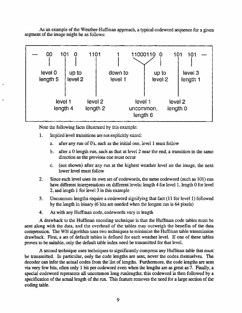
As an example of the Weather-Huffman approach, a typical codeword sequence for a givensegment of the image might be as follows:

00 101 0

I I1101 1

I11000110 0

I101 101

Ilevel 0

length 5up to

level 2down tolevel 1

up tolevel 2

level 3length 1

level 1length 4

level 2length 2

level 1uncommon,

length 6

level 2length 0

Note the following facts illustrated by this example:

1. Implied level transitions are not explicitly stated:

a. after any run of O's, such as the initial one, level I must follow

b. after a 0 length run, such as that at level 2 near the end, a transition in the samedirection as the previous one must occur

c. (not shown) after any run at the highest weather level on the image, the nextlower level must follow

2. Since each level uses its own set of codewords, the same codeword (such as 101) canhave different interpretations on different levels: length 4 for levell, length 0 for level2, and length 1 for level 3 in this example

3. Uncommon lengths require a codeword signifying that fact (11 for level 1) followedby the length in binary (6 bits are needed when the longest run is 64 pixels)

4. As with any Huffman code, codewords vary in length

A drawback to the Huffman encoding technique is that the Huffman code tables must besent along with the data, and the overhead of the tables may outweigh the benefits of the datacompression. The WH algorithm uses two techniques to minimize the Huffman table transmissiondrawback. First, a set of default tables is defined for each weather level. If one of these tablesproves to be suitable, only the default table index need be transmitted for that level.

A second technique uses techniques to significantly compress any Huffman table that mustbe transmitted. In particular, only the code lengths are sent, never the codes themselves. Thedecoder can infer the actual codes from the list of lengths. Furthennore, the code lengths are sentvia very few bits, often only 1 bit per codeword even when the lengths are as great as 7. Finally, aspecial codeword represents all uncommon long runlengths; this codeword is then followed by aspecification of the actual length of the run. This feature removes the need for a large section of thecoding table.

9

2.2 RUNLENGTH FILTERING AND RESOLUTION REDUCTION

If the Huffman runlength encoding of the exact input weather image requires more than theallowable number of bits, some fonn of detail reduction must be perfonned on the image to lowerthe encoding load. Two types of image simplification are used as part of the WH approach:runlength flltering and resolution reduction.

Isolated weather pixels add substantially to the Huffman runlength encoding requirement.For example, the following sequence of pixels - 221222 - produces code for 3 runs and 2 levelchanges. By changing the isolated pixel to a 2, the encoding reduces to that for a single run.Altering the weather level of such isolated pixels is in some cases deemed acceptable distortion forthe large benefit in data compression that is achieved.

In the example of the NEXR.AD radar graphic, for pilot safety considerations, no reductionin level is pennitted for moderate (level 2) or greater pixels in the filtering operation; only level 1pixels may be reduced. Any weather level pixel, however, may be increased a single increment byfIltering, and in addition level 0 pixels may be set to level 2. Thus, examples of the application andrejection offiltering operations are:

(a) 11011 -> 11111 0 can increase

(b) 33433 -> 33433 4 can't be reduced

(c) 12033 -> 12233 0 can be raised to 2

(d) 11233 -> 11233 no gain by changing the 2 to 3

(e) 101010 -> 111111 preferraisingOtoloweringl

Another, more severe, way to decrease the Huffman runlength encoding bit requirementsof a weather image is to reduce the resolution of the image from 256x256 pixels to 128x128 pixels,with each new pixel representing 4 of the old ones (a 2x2 square). This change produces ablockier image, but maintains reasonable fidelity. If this reduction is not sufficient to satisfy the bitlimit, further reduction to 64x64 pixels, or even 32x32 pixels, is utilized in the WH algorithm.

The approach chosen to produce the various size superpixels emphasizes higher levels ofweather, in that the new pixel setting is influenced most by the highest weather level in thesuperpixel square. The level chosen also depends upon the weather in the neighboringsuperpixels, in that no region of weather of level 3 or above, even if only 1 pixel in size, will everbe pennitted to be lost via resolution reduction.

2.3 SMOOTHING PROCESS

Whenever the Weather-Huffman encoding requires resolution reduction of the input imageto meet the datalink bit limitation, the decoder must expand the received image back into its fullresolution. Without any other infonnation about the original image to go by, the decoder isreduced to replicating each received superpixel into 4 quadrants of same~levelpixels at each step ofthe regeneration. Thus, if a received superpixel were of size 4x4, the decoder would generate 42x2 superpixels, and then 16 lx1 actual pixels, all of the same weather level The result of thisoperation is the generation of an output image with weather regions that are larger and blockier thanthose on the input image.

10

;

The Smoothing Process attempts to mitigate this effect by using knowledge of weatherregion shapes to reduce in level some of the pixels at each regeneration step. For example, weatherregions do not often have sharp comers. The Smoothing Process, for reasons of pilot safety, isnot allowed to reduce the extent of weather regions. It is only permitted to reshape the edges ofregions to drive them closer to expected reality.

2.4 EXTRA BIT ALGORITHM (EBA)

Should the Huffman coding of the Hilbert-scanned input image produce too many bits tomeet the datalink limit, the Huffman encoding will need to be applied to a reduced resolutionversion of the input image, with pixels replaced by superpixels (2x2, 4x4, or 8x8). Then thedecoder will expand each received superpixel into an array of pixels, each with the same leveLThis will result in output weather regions being noticeably larger and more blocky than those onthe input image. While the smoothing algorithm attempts to reduce this effect, it has two majordrawbacks:

1. only a few pixels are subject to level reduction, and

2. the smoother makes its reduction without any knowledge of the actual weathercontours

In effect, the smoothing algorithm uses knowledge of typical weather region shapes to

produce a more esthetically pleasing result, which is usually, but not guaranteed to be, moreaccurate than the decoder output

The Extra Bit Algorithm (EBA) utilizes the bits remaining in the uplink message to relate tothe decoder correction infonnation for selected quadrants of as many superpixels as possible. Theinfonnation, one bit per quadrant,. says either to leave the quadrant at the superpixel level or toreduce the quadrant by 1 weather leveL Successive applications to the same quadrant, via morethan one pass through EBA, can achieve greater than 1 level reductions, and quadrants that wereincorrectly smoothed down can be returned to their original correct values.

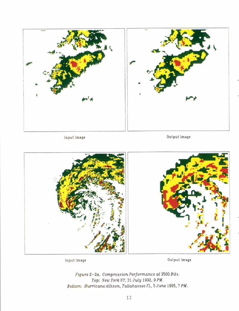
2.5 SAMPLE IMAGE RESULTS

Weather images representing light weather conditions require no compression to meet a3500 bit limit Figures 2-2a and 2-2b illustrate the performance of the Weather-HuffmanAlgorithm on images that do require compression, namely severe weather images (the worst wecould fmd) produced at various U.S. locations. The first and last images were taken in the NewYork area, the third at Mobile, and the second represents hurricane Allison at Tallahassee.

Each image is 256x256 pixels, with a pixel representing 2 kilometer by 2 kilometers; thuseach image covers a region approximately 300 nautical miles on a side. The figure' in each casecompares the input weather image to the output image provided the pilot.

It was required in each case that the WH algorithm input at least a 4x4 resolution-reducedimage to the runlength encoder (the last image required 8x8 reduction because of its extremely largenumber of small heavy weather regions). This level of reduction appears typical for severeweather images. However, the output images were in each case quite reasonable representations of"truth". Some blockiness and region blooming are apparent in each output, though the fidelity wasjudged operationally acceptable in each case.

11

•

Input Image Output Image

;..:

f. r

;~

Input Image Output Image

Figure 2-2a. Comp'ression Performance at 3500 Bits.Top: /lew York NY, 31 July 1992, 9PM.

Bottom: Hurricane ALLison, TaLLahassee FL, 5 June 1995, 7 PM.

12

•

..-.:

•• •

••• •

-..

r '7 ....

r ....~ • ...

~ .•r. "..."'''';.' ..>

Input Image Output lmage

Input Image Output Image

Figure 2-2b. Compression Performance at 3500 Bits.Top: MobileAL, 11 May 1995, 6 PM.

Bottom: Bridgeport CT, 11 May 1995, 6 PM.

13

Based on the results seen to date on a large number of weather images, it appears that theWeather-Huffman Algorithm is successful in providing accurate weather images to pilots over bit­limited datalinks.

2.6 PROGRAM SIZE AND TIMING MEASURES

The Weather-Huffman algorithm has been fully coded in the C language and tested on aDigital Equipment Corporation MicroVAX 3500 Color Graphics Workstation. (The 3500 is aminicomputer whose performance can be matched or exceeded by modem high-capability 32-bitmicrocomputers). Considerable effort has been made to optimize the coding for computationalefficiency.

The compression routines start with a 256x256 pixel image array (read from a disk me) andproduce a bit-string in memory. The decompression routines perform the inverse transfonnation.The WH algorithm requires about 2 megabytes of memory to execute its compression procedureand about 1 megabyte of memory to execute its decompression procedure. This includes all code,data areas, and C libraries used.

The algorithm was tested on a set of severe weather images derived from data supplied byweather services. Timing the procedures was done with the VAX system clock, accurate to a 10millisecond quantization. All testing assumed a 3500 bit limit The algorithm, as presently codedand run, requires about 3 seconds on average to encode these severe images. (Tests on moretypical weather images required significantly less time per image). The decoding routines, on theother hand, require only 0.35 seconds processing per image.

It is clear that the processing requirements for the airborne datalink computer to performdecoding for the WH algorithm is quite reasonable:

onboard memory: 1 megabyte

onboard processing: 0.35 seconds per image

The speed-optimized WH algorithm requires more computer resources to do its encodingprocedure, but, its requirements are still reasonable for modem ground-based computer systems.

14

3. HUFFMAN RUNLENGTH CODING

Coding theory tells us that if successive runlengths are independent random variables, themost efficient codes for representing them are entropy codes. Entropy codes are those whosecodeword lengths are based on the frequency of occurrence of the symbol being encoded; morecommon runlengths will be assigned shorter codewords. In order for variable length codes to beuniquely decodable, their codewords must satisfy the prefix constraint: no codeword can be theprefix of any other codeword.

The most efficient entropy prefix code is the Huffman code. This code assignment isoptimum in the sense that the total number of bits required to transmit a set of runlengthsdescribing a given random image is minimum. Unfortunately, since the code assignment will bedifferent for each image, the Huffman approach requires the overhead of transmitting a decodingtable as part of each encoded message. This overhead can easily eliminate the optimality of theHuffman approach

The Weather-Huffman algorithm is a modification of the standard Huffman encodingscheme, with weather runs being the entities to be encoded. It introduces variations to reduce thenumber of bits required for encoding such images, particularly concentrating on methods ofreducing the decoding table overhead. In order to help the reader understand the WH approach,this section presents the details of the general Huffman algorithm. The next section then providesdetails of the Weather-Huffman modifications.

3.1 IMAGE SCANNING PROCEDURES

A run on a weather image is a number of successive pixels having the same weather level.In order to determine a run, the term "successive" must be defined. The "normal" method ofscanning a 2-dimensional picture is the raster scan, which proceeds left-to-right, row-by-rowdown the picture. The raster scan takes advantage of the continuity, or smooth edge, property ofweather regions. That is, successive rows will tend to have similar run characteristics, whichmakes the Huffman coding job more efficient.

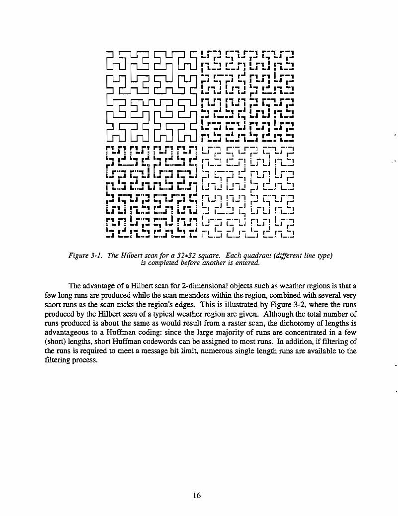
An alternative scanning method, the Hilbert scan, exploits a different property of weatherregions, namely their contiguity, or tendency to form large 2-dimensional areas. The Hilbert scanis a 2-dimensional space-filling scan with the property that all pixels in a binary 2D square arevisited before that square is left The Hilbert scan for a 32*32 square can be seen in Figure 3-l.Note that, as just stated, each quadrant is completed before the next quadrant is entered.

15

r ...... r ........., .., r ....,: .. .1:: .. .1:: .. .1:: .. .1:L.. ,'" L.. r'" L.. r'" L.. r'"r.l _.I "Ill ... .1 _.I "Ill

: r , I : r , IL .I L L .I L .I.., L r" .., L .I r"I I. 1.1 Lo II. ., , r r"r" L, r" .., L.. r.l ..,: .. , : r" .., r" .., : , .. :L" .... : L : L.. L'"r, .., I , I , .. r.,: .. .I : r" .., L.. : L.. :L.. r'" r" .., r" .., L., .. .I_.. "_Ol L ~_.. L_

I ..-, r-" r-....-, ..-,.... r~ .., L.. r" L~ .. .I r"r" .., r" .., I .. , I r" "II L_~ .._J I L_..... r--" r..l "I I ..-,po" .. , po" .. , I I .... r~

I r" I I r" I L.. rOIl r" "IL.. LOll L.. LOll _ .. L_..r" r" r" r" -., ..-,I L.. I I L.. I r" L~ .... r".., .. .I .., ...I I .. , I r" ..,... L_... L, L_..I r-" ..-, I ..-,L I .. .I I r".. , L r" L.. rOIl r" "II .. _J L_.. L_" .._.. L_...

Figure 3-1. The Hilbert scan for a 32*32 square. Each quadrant (different line type)is completed before another is entered.

The advantage of a Hilbert scan for 2-dimensional objects such as weather regions is that afew long runs are produced while the scan meanders within the region, combined with several veryshort runs as the scan nicks the region's edges. This is illustrated by Figure 3-2, where the runsproduced by the Hilbert scan of a typical weather region are given. Although the total number ofruns produced is about the same as would result from a raster scan, the dichotomy of lengths isadvantageous to a Huffman coding: since the large majority of runs are concentrated in a few(short) lengths, short Huffman codewords can be assigned to most runs. In addition, if fIltering ofthe runs is required to meet a message bit limit, numerous single length runs are available to thefiltering process.

16

Long Meandering Run:Runlength 33 Pixels

Short IINickll Runs:tr~--+-

Runlengths 1 Pixel

Figure 3-2. The Hilbert scan of a typical weather region. Several long meanderingruns and several short "nick" runs are produced.

This assertion was tested by processing 11 sample NEXRAD weather images via bothscanning methods. The ensemble average number of bits required by the Huffman runlengthencoding were as follows:

Scanning Method

Raster

Hilbert

Input Image

22546

20179

4x4 Filtered Image

2444

2168

Thus, the Hilbert scan saved an average of 10% for the unedited images, and 11% for thefiltered images. Considering the fixed decoding table overhead, these savings, particularly thelatter one, are quite substantial.

17

The generation program for the Hilbert scan can be expressed in the following iterativefonn:

Hilbert(i)

{

hilbert1Ce','s' ,'w','n' ,i);

}

hilbert1(r,u,l,d,i)

{

if(i>O)

{

hilbert! (u,r,d,l,(i-l»;

move(r);

hilbertl(r,u,l,d,(i-l»;

move(u);

hilbert1(r,u,l,d,(i-l»;

move(l);

hilbertl(d,l,u,r,(i-l»;

}

}

/* main routine */

/* subroutine */

/* iterative calls to itself */

where 'e','s','w','n' are the directions of the compass, the move function tells you tomove in the direction of its argument, and

i =log2(n) (i =8 for a 256x256 image).

Note that the iterative calls to hilbertl have various permutations of the original arguments;this is what causes the reflections and rotations of the curve components.

3.2 CODEWORD DETERMINATION

The Huffman algorithm takes as its input a non-increasing list of runlength probabilities.At each step, it combines the two lowest entries on the list into a single new entry. The twomerged entries are removed, and the new entry is sorted into its proper location to create a newshorter ordered list. The process tenninates when only a single entry remains. The record of pairmergings is then used to construct a binary tree which specifies the Huffman codewords in themanner now to be explained.

18

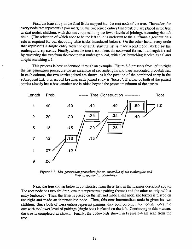
First, the lone entry in the final list is mapped into the root node of the tree. Thereafter, forevery node that represents a pair merging, the two joined entries that created it are placed in the treeas that node's children, with the entry representing the fewer levels of joinings becoming the leftchild. (The selection of which node to be the left child is irrelevant to the Huffman algorithm; thisrule is required for our decoding table tricks introduced below). On the other hand, every nodethat represents a single entry from the original starting list is made a leaf node labeled by therunlength it represents. Finally, when the tree is complete, the codeword for each runlength is readby traversing the tree from the root to that runlength's leaf, with a left branching labeled as a 0 anda right branching a L

This process is best understood through an example. Figure 3-3 presents from left to rightthe list generation procedure for an ensemble of six runlengths and their associated probabilities.In each column, the two entries joined are shown, as is the position of the combined entry in thesubsequent list. For record keeping, each joined entry is "boxed"; if either or both of the pairedentries already has a box, another one is added beyond the present maximum of the entries.

Length Prob. ------- Tree Construction Root

7 .12

5 .15

1 .07

II .60 II 1.0

.40 5V.20

.404

9 .06

2

Figure 3-3. list generation procedure for an ensemble of six runlengths andtheir associated probabilities.

Next, the tree shown below is constructed from these lists in the manner described above.The root node has two children, one that represents a pairing (boxed) and the other an original listentry (unboxed). Thus, the latter is placed on the left and made a leaf node, the former is placed onthe right and made an intermediate node. Then, this new intermediate node is given its twochildren. Since both of these entries represent pairings, they both become intermediate nodes; theone with the lower level of pairings (single box) is placed on the left. Continuing in this manner,the tree is completed as shown. Finally, the codewords shown in Figure 3-4 are read from thetree.

19

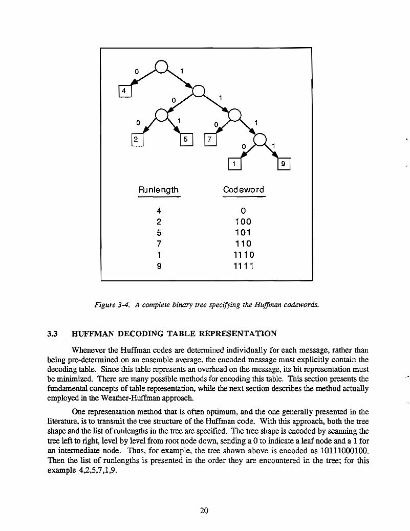
RJnlength Codeword

4 02 1005 1017 1101 11109 1111

Figure 3-4. A complete binary tree specifYing the Huffman codewords.

3.3 HUFFMAN DECODING TABLE REPRESENTATION

Whenever the Huffman codes are determined individually for each message, rather thanbeing pre-determined on an ensemble average, the encoded message must explicitly contain thedecoding table. Since this table represents an overhead on the message, its bit representation mustbe minimized. There are many possible methods for encoding this table. This section presents thefundamental concepts of table representation, while the next section describes the method actuallyemployed in the Weather-Huffman approach.

One representation method that is often optimum, and the one generally presented in theliterature, is to transmit the tree structure of the Huffman code. With this approach, both the treeshape and the list of runlengths in the tree are specified. The tree shape is encoded by scanning thetree left to right, level by level from root node down, sending a 0 to indicate a leaf node and a 1 foran intermediate node. Thus, for example, the tree shown above is encoded as 10111000100.Then the list of runlengths is presented in the order they are encountered in the tree; for thisexample 4,2,5,7,1,9.

20

Upon reception, the decoder constructs the tree from the shape specification, knowing thatevery intennediate node will have two children. Every time a leaf node is encountered, the nextrunlength is read from the runlength list and its code read by traversing the tree to its position.This approach to decoding table presentation requires at most 2n bits for the tree specification,where n is the number of runlengths, plus n*m bits for the runlength list, where the longestrunlength L satisfies L :;:; 2m.

A more straight-forward, though more bit-eonsuming, method of representing the decodingtable is to list the n triplets of runlength, number of codeword bits, and codeword. Thus, the tablefor the above example would be the following:

number of runlengths n =6

runlength number of bits

1 4

2 34 1

5 3

7 3

9 4

codeword

1110

100

o101

110

111

This manner of representation can be shortened considerably by leaving out the entire thirdcolumn. This "trick" can be performed because it is possible, with our tree rules described above,to infer the codeword from its number of bits through use of the following algorithm:

1. Reorder the runlengths in increasing order of number of bits; if two or more have thesame value, list them in the order in which they appear in the decoding table.

2. Initialize:

bi =number of bits of fIrst runlength

codel =bi bits of 0

3. Compute each other codeword from the previous one:

bi = number of bits of runlength i

codei = (codei_I + 1) followed by (hi - bi-I) D's

Applying this algorithm to the above example, the re-ordered list of runlengths wouldbecome 4,2,5,7,1,9. Then, for instance, the code for a runlength of 1 (i=5) is generated from thecode for a mnlength of 7 (i=4) as follows:

codes =(code4 + 1) followed by (bs - b4) O's

=(110 + 1) followed by (4 - 3) D's

=1110

Proceeding in this manner, all the codes shown above would be produced.

21

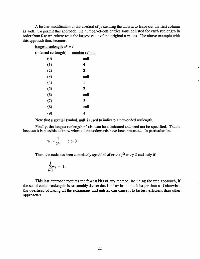
A further modification to this method of presenting the table is to leave out the first columnas well. To permit this approach, the number-of-bits entries must be listed for each runlength inorder from 0 to n*, where n* is the largest value of the original n values. The above example withthis approach thus becomes:

long;est runleng;th n* = 9

(inferred runlength) number of bits

(0) null

(1) 4

(2) 3

(3) null

(4) I

(5) 3

(6) null

(7) 3

(8) null

(9) 4

Note that a special symbol, null, is used to indicate a non-eoded runlength.

Finally, the longest runlength n* also can be eliminated and need not be specifIed. That isbecause it is possible to know when all the codewords have been presented. fu particular, let

Then, the code has been completely specilled after the jth entry if and only if:

This last approach requires the fewest bits of any method, including the tree approach, ifthe set of coded runlengths is reasonably dense; that is, if n* is not much larger than n. Otherwise,the overhead of listing all the extraneous null entries can cause it to be less efficient than otherapproaches.

22

To overcome this efficiency problem, a hybrid approach is possible when many shortrunlengths, but only a few scattered longer runlengths, exist. The hybrid approach starts with asequence of inferred-length number-of-bit entries from 0 to n/, followed by the remaining entriesgiven by a series of explicit runlength and number-of-bits pairings. The above example might thenbe presented as follows:

lQncest sequential runlencth nl =5

(inferred runlength) number Qf bits

(0) null

(1) 4

(2) 3

(3) null

(4) 1

(5) 3

runlencth

7

9

number Qf bits

3

4

Note that the number Qf explicit runlengths need not be specified because Qf the enddetenninatiQn rule given abQve. A modification of this last method, described in Section 4 , is theapproach used by the Weather-Huffman algorithm.

23

4. WEATHER-HUFFMAN CODING TABLE

The Huffman theory section presented general methods for creating the codewords to beused in encoding weather runlengths, as well as alternatives for transmitting to the decoder thetables specifying the chosen nmlengthlcodeword pairings. This section develops the specializedtechniques developed for the Weather-Huffman (WH) application that result in a major reduction inthe number of bits needed to transmit the Huffman tables. In fact, it is these enhancements thatmake the WH approach feasible as a data compression algorithm for the Mode 5 data link; with the"normal" approach, the decoding tables alone could on occasion exceed the bit capacity of theMode 5 message.

4.1 REPRESENTATION OF LONG RUNLENGTHS

Providing a separate codeword for every nmlength existing for a given image level wouldgenerally be very inefficient because of the large decoding table overhead, even· if the hybridapproach to table representation described in the theory section were adopted. Thus, the Weather­Huffman algorithm makes use of two special codewords to represent "other" length runs, where"other" is defmed as any length beyond the longest one explicitly given a codeword. These wordsobviate the need to list numerous explicit runlengths and their codeword lengths.

The frrst special codeword (denoted by 51), when encountered, informs the decoder thatthe next set of bits will state the actual length of the run; in the simplest implementation these extrabits would just be the binary value of the length (i.e.: ()()()UO = 6). 5ince the longest possiblerunlength is 65536 (for a 256x256 image), 16 bits would be required for the extra field every timean "other" length occurs.

To reduce this overhead to only 6 bits, only lengths up to 63 are represented by the specialcodeword 5 1. Longer lengths are encoded by the use of a second special codeword (52); thiscodeword tells the decoder that a run of greater than 63 pixels is present. The decoder then recordsthe initial length 63 part of the run, doesn't change level, and reads the length of the remainder ofthe run in the normal manner. For example, a run of 149 would be encoded as follows:

(word 52) (word 52) (word 51) (binary 23)

63 + 63 + 23 == 149

if a run of 23 were an "other" length.

4.2 ENCODING "OTHER" LENGTH RUNS

Even using only 6 bits for specifying the length of "other" runs is inefficient when theseruns are generally at the short end of the spectrum. Thus, the Weather-Huffman implementationconsiders the use of shorter binary fields on a level-by-level, image-by-image basis. It does thiseither by uniformly reducing the number of bits if the longest runlength is sufficiently short tomake this possible, or by employing a "long-short" dichotomy for the set of runlengths otherwise.

With a "long-short" scheme, short runs use fewer specification bits than do long runs; asingle extra bit preceding the binary field indicates which bitlength applies. The long-shortapproach makes sense when most of the "other" runs are at the short end of the spectrum, as then

25

Rmax.+LiLRj*<Ei+BLJ

j=Rmax.+Si+1

the loss encountered by having to include the extra bit is more than offset by the gain of havingnumerous short specifications.

The full set of options utilized by the Weather-Huffman algorithm, including both uniformbit reduction and long-short approaches, for the representation of "other" lengths for a given imagelevel are as follows:

Option Bit Field Lengths Extra Bit Needed

0 6 no

1 6 3 yes

2 6 2 yes

3 5 no

4 5 2 yes

5 4 no

6 3 no

7 2 no

For example, with option 1, a long-short scheme, "other" runs that are 8 pixels or fewergreater than the longest explicitly specified runlength will require a 3-bit binary field (plus thesingle extra bit); longer runlengths will require 6 + 1 bits. Conversely, with option 5, a uniformreduction method, all runlengths are specified by 4 bits, but the longest "other" run must notexceed the longest specified length by more than 16 for this option to be applicable. The option inuse for each level will, of course, have to be included in the transmitted decoding table.

Once the longest runlength Rmax to be explicitly coded is determined (by the methoddiscussed below), selecting the proper long-short option to employ is quite simple: try all eight,and choose the one requiring the fewest bits to encode all the "other" runs. In particular, the"other" bit requirement for option i is given by:

Rmax+SiI,Rj*<Ei+BSi) +

j=Rmax+l

where Rj is the number of runs of length j, Si and Li are the number of runlengths accommodatedby the short and long bit fields, respectively, for option i, BSi and BLi are the number of bits in theshort and long fields, and Ei is 1 if the option uses a long-short dichotomy:

Option BSi Si LSi Li Ei

1 0 6 64 02 3 8 6 64 13 2 4 6 64 14 5 32 05 2 3 5 32 16 0 4 16 07 0 3 8 08 0 2 4 0

26

Note that an option i is not a viable candidate if the longest runlength for the image levelexceed Rmax + Li, which is the longest runlength that can be represented by the option.

4.3 ELIMINATION OF LONG CODEWORDS

Since for any given image level there are 66 potential runlengths to be assigned codewords(0-63, SI, S2), it is quite possible for the Huffman algorithm to produce codewords that exceedsthe desired 7 bit limitation. (1be theoretical limit is 65 bits, but a weather image does not containenough pixels to ever approach that value). In these cases, the codewords must be modified tosatisfy the imposed limit In particular, some of the shorter codewords must be lengthened topennit the outlier codewords to be brought down within the 7 bit limit

The algorithm adopted is, when a choice exists, to start by modifying codewords of length6, then proceeding if necessary to codewords of length 5, etc. until all the longer codewords havebeen brought down to length 7. This approach, of not lengthening any codeword for commonrunlengths, minimizes the number of bits required for image encoding.

When the longest codeword is restricted to have at most 7 bits, there are 27 = 128 bitsequences in the code space. Each codeword of length m, because of the prefIx nature of theHuffman code, exhausts 2(l-m) of these sequences. For example, the codeword 01001 removesthe sequences 0100100,0100101,0100110, and 0100111 from possible assignment, while any 7bit codeword removes only its own sequence from the available list

This realization has led to the following algorithm for the reassignment of Huffman codeswhen the longest codeword produced by the Huffman algorithm exceeds the 7 bit limit, where thecodewords are ordered from the shortest to the longest:

1. Initialize i =0, and let n =number of codewords.

2. Initialize the number of sequences used to U =o.3. Increment i by 1; if i > n, quit.

4. Increase U by 2(7-bi), where bi =number of bits currently assigned to codeword i.

5. If (128 - U) =(n-i), set bj =7 for all j =i+l, ... ,n; quit.

6. Otherwise, if (128 - U) < (n-i), repeat the following actions:

a. increment bi by 1

b. adjust U =U - 2(7-bi+l) + 2(7-bi)

until (128 - U) ~ (n-i), then return to step 3.

7. Otherwise, if (128 - U) > (n-i), repeat the following actions:

a. compute A =2(l-bi+l) - 2(7-bi)

b. if (128 - U - A) ~ (n-l),

decrement bi by 1 and adjust U = U + Auntil the test in b fails, then return to step 3.

Step 5 recognizes the fact that if the number of remaining sequences and remainingrunlengths are equal, each remaining runlength can be assigned a 7-bit codeword. Step 6 handles

27

Adjusted Length

1

2

3

5

5

7

7

7

7

7

7

7

7

Huffman Length

1

2

3

4

6

6

6

7

8

9

10

11

11

the case that fewer sequences than runlengths remain, so that more available sequences have to begenerated by increasing the length of the codeword assigned to the current runlength. Finally, step7 recognizes the case when previous applications of step 6 have freed up more sequences thanwere required, so that the codeword for runlength i may be able to be decreased to absorb some ofthe extra sequences.

An example of the application of this algorithm is given by the following before and afterset of codeword length assignments:

Runlength Order

1

2

3

4

5

6

7

8

9

10

11

12

13

Note that the 4th runlength had to have its codeword length increased to accommodate thecodewords over the limit, but that by doing so the number of sequences freed up also allowed the5th codeword to be shortened.

4.4 WEATHER-HUFFMAN (WH) TABLE ENCODING

The actual Huffman table encoding employed by WH can now be described. The generalmethod utilized is a variant on the implicit runlength scheme presented in the previous section, inwhich a list of codeword lengths (with null meaning no codeword because that runlength neveroccurred) is presented. The order of the implicit runlengths is Sl, 52,0, 1, 2, 3, .. , , n, where nis the longest encoded runlength, and thus (n+1) is the first "other" length. Since the null length isexpected to be the most common encoded value, the runlength codes are encoded in two parts: asingle bit indicating null (0) or not null (1), and a field for the non-null cases which presents theactual length of the Huffman code for that runlength.

The simplest way to present the latter field would be to set a limit on the acceptable lengthof a Huffman codeword, and then use enough bits in the field to cover all possible values of thatmaximum length. For example, if the limit is set at 7, 3 bits would be required for the field. Notethat limiting the codeword length required the modification to the codeword generating algorithmpresented above to cover the cases when the algorithm produces longer codewords.

28

Rather than use a constant length field, the Weather-Huffman algorithm saves bits bycomputing, for each runlength, the set of codeword lengths that could possibly still exist. This setcan be determined from the previously listed codeword lengths if the longest codeword for thelevel is known and the rule given earlier,

I

I

1

variable

variable

variable

variable

No. of Bits

2

3

1

bi > 0 is used. The specific algorithm for encoding the codeword lengths is1

where Wi = -bo2 1

provided below.

Putting together all of the above pieces, the Huffman table for each image level is presentedas the following set of fields:

Field

Table present (Le., non-default)

Longest codeword used

Sl encoded?

if yes, S1 codeword length

S2 encoded?

if yes, S2 codeword length

Length 0 encoded?

if yes, 0 codeword length

Length 1 encoded?

if yes, 1 codeword length

Length n encoded? 1

if yes, n codeword length variable

if S1 encoded, option used 3

As described below, three default codeword sets are available for each image level. Thetrrst two bits above either specify one of these default sets, in which case the table specificationterminates, or state that the actual table description is to follow. The codeword-reading process isknown to be over when the completion rule above is satisfied, that is, when the length n has beenread such that:

~;;=1~

29

Also, for image levels 0 or mapmax, no runs of length 0 can exist; thus that length is notencoded.

4.5 ENCODING CODEWORD LENGTHS

The concept of counting the number of "used" sequences presented earlier can also beapplied advantageously to the problem of determining how many bits are required to encode thelengths of codewords in the decoding table. If the length of the longest codeword used for a givenimage level is stated to be Lmax, then the length Ll of the fIrst codeword presented in the table isrestricted to the range:

Ll =0 ifLmax =0

ifLmax >0

Note that if a Q-length codeword is used, it must be the only codeword for that level since itwould use up all 128 available sequences; thus knowing another length Lmax exists precludes the 0length.

After each codeword length is specilled in the decoding table, the number of availableunused sequences decreases. Thus the range of possible codeword lengths also decreases as one­by-one the shorter lengths drop out as possibilities. In particular, by the formulas of the lastsection, length L is still an option only if:

2(7-L) ~ (128 - U)

As the set of codeword length options decrease, of course, the number of bits needed in thedecoding table to specify the actual length will also decrease (in fact, if only 1 option remains, nobits at all are needed!). For example, consider the codeword length assignments in the followinglist of runlengths when the longest codeword is stated to be 4:

Sequences Runlength Code Length Bits Needed to Actual CodeUsed So Far Options Specify Length Used

0 1 1-4 2 3

16 2 1-4 2 248 3 1-4 2 280 4 2-4 2 2

112 5 3-4 1 4

120 6 4 0 4

where the sequences used so far entry is increased at each step according to the length used in thelast column of the previous row. The total of the bits needed to specify column represents asavings of 50% over the 3 bits per codeword length that would be required by the "normal"approach when a 7-bit codeword limitation is enforced.

The bit requirement for specifying the codeword length can be reduced even further byemploying a Huffman approach (Huffman encoding the entries of the Huffman decoding table!).For example, if the code length options available at a given point are 5, 6, and 7, it takes 2 bits for

30

i =SI, S2, 0, 1. ...• n

the specification by the above logic. But it is possible to shorten the specification for length 7 bychoosing the following set of decoding table entries:

5: 11

6: 10

7: 0

In particular, whenever the number of options is not fully 2m, some of the options can beassigned m-l bits for their specification. The WH algoritlun in such cases assigns the I-bit shorterm-l bit specifications starting with length Lmax, then with Lmax-l, etc. until only m bitsspecifications are available.

Complete details of the encoding and decoding of the decoding table are presented inSections 8 and 9, respectively.

4.6 DETERMINING THE "OTHER" LENGTH BREAKPOINT

The final piece of the decoding table puzzle is how to detennine the longest runlength toexplicitly give its own codeword, with the remaining longer runlengths relegated to the "other"category. In a pure Huffman coded system, the "optimum" codewords would be detennined asoutlined in the theory section, with each length assigned its own codeword. However, therequirement of transmitting the decoding table in the message changes the problem fromminimizing the total codeword bits to instead:

Problem: Minimize T ={(Table bits) + (Codeword bits) }

With the table architecture described earlier, the only variable that affects the minimizationproblem is Lmax, the longest explicitly encoded runlength. Since providing each runlength with itsown codeword will always minimize the number of bits needed to encode the weather runs, thetradeoff when changing Lmax can be expressed by:

as Lmax is raised, the bits for encoding runs decreases, but

as Lmax is raised, the decoding table size increases.

The optimum value ofLmax is the value that minimizes the sum of encoding bits and tablebits.

Because of all the "tricks" used to represent the decoding table, there is no simplecalculation that will produce the optimum value of Lmax. If the optimum is truly sought, all valuesof Lmax from 0 to the longest runlength must be processed through both the Huffman codewordassignment and the table generation algorithm to learn the number of bits required for that value;the smallest total found then detennines Lmax.

For a given value of Lmax, the computation ofT proceeds as follows:

631. Let R6s = I. Ri be the number of "other" runs.

i=n+l

2. Detennine the Huffman codewords Ci for the lengthsusing the frequencies Ri.

31

4. Detennine the "other" option number that minimizes the bits T2 required to state theexplicit second codewords for the "other" runlengths (if Rt55 = 0, Tl = 0).

5. Detennine T3, the number of bits required to encode the Huffman table for this valueof n.

6. T=Tl+T2+T3.

If this calculation is perfonned for all values of Lmax, the minimum value Tmio will bedetennined.

Clearly, this process is very time consuming, and a shortcut that eliminates many of theLm.ax values from consideration would be highly desirable. The method adopted to attain this goalis to not test any value i if its number of runs Ri satisfies either

(a) Ri < Ri+1. or

(b) Ri ~ 1

If the first condition applies, the next runlength value will probably be a better stoppingpoint than this one; if the second condition applies, this runlength value will probably not beat thecurrent optimum stopping point. The length Rmax. is always tested even if it has only 1 run, as theelimination of the need for "other" runs is a significant savings of bits.

4.7 DEFAULT CODE ENSEMBLES

The above "tricks" for encoding the Huffman decoding table have severely reduced the bitrequirements of these tables. In fact, tests on sample images show that often as few as 20 bits areneeded for a table for a particular weather leveL

Alternatively, a default Huffman codeword set can be employed for the level. Thepredefined codewords will generally not be optimal for the level's actual runlength statistics, butthe elimination of the need for the decoding table can result in fewer total encoded bits. TheWeather-Huffman algorithm has defmed 3 default codeword sets for each weather level, matchedto statistics found on a set of test images. These default sets, which vary by level, are presented inAppendix A. Since each default set has a defmed value of Lmax, the approach given above can befollowed to determine for each set the number of bits Tdef,i that are required if it is selected for theencoding. The only differences are that step 2 is avoided (the default codewords are used) and instep 5, T3 = 5 (2 bits for the default number and 3 bits for the option selection). The default setwith the smallest result is the winner, with Tdef being its calculated value.

Finally, the proper encoding scheme for each level is found by comparing the table-drivenvalue of Tmio to the optimum default-driven value of Tdef. If the latter if smaller, the encodersimply lists the number, 0, 1, or 2, of the optimum default option; if the former is smaller, theencoder lists the value 3 followed by the decoding table.

32

5. WEATHER IMAGE SIMPLIFICATION

If the Huffman runlength encoding of the exact input weather image requires more than theallowable number of bits, some form of detail reduction must be performed on the image to lowerthe encoding load. Two types of image simplification are used as part of the Weather-Huffmanapproach: runlength filtering and resolution reduction.

5.1 RUNLENGTH FILTERING

Isolated weather pixels add substantially to the Huffman runlength encoding requirement.For example, the following sequence of pixels - 221222 - produces code for 3 runs and 2 levelchanges. By changing the isolated pixel to a 2, the encoding reduces to that for a single run.Altering the weather level of such isolated pixels is in some cases deemed acceptable distortion forthe large benefit in data compression that is achieved.

For pilot safety considerations, no reduction in level is permitted for significant weatherpixels (level 2 and above) in the filtering operation; only level 1 pixels may be reduced. Anyweather level pixel, however, may be increased a single increment by filtering, and in additionlevel 0 pixels may be set to level 2. Thus, examples of the application and rejection of filteringoperations are:

(a) 11011 -> 11111 ocan increase

(b) 33433 -> 33433 4 can't be reduced

(c) 12033 -> 12233 0 can be raised to 2

(d) 11233 -> 11233 no gain by changing the 2 to 3

(e) 101010 -> 111111 prefer raising 0 to lowering 1

(f) 33133 -> 33233 1 can only be raised to 2

Example (d) recognizes the fact that a sequence of 11333 would still require a 0 length runspecification for level 2, and hence no gain would be achieved by making the change. Similarly,example (f) saves the two 0 length runs that would have been required for level 2, one on thedescent and the other on the subsequent ascent.

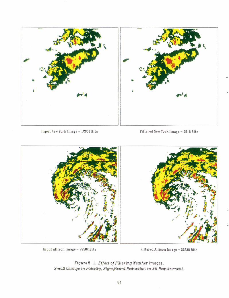
Figure 5-1 presents before and after views of the fIltering operation for two typical weatherimages. Note that the significant reduction in bit requirement for the Huffman encoding isachieved at a very minor distortion in the weather regions on the image.

5.2 RESOLUTION REDUCTION

Another, more severe, way to decrease the Huffman runlength encoding bit requirementsof a weather image is to reduce the resolution of the image from 256x256 pixels to 128x128 pixels,with each new pixel representing 4 of the old ones (a 2x2 square). This change produces ablockier image, but maintains reasonable fidelity. If this reduction is not sufficient to satisfy the bitlimit, further reduction to 64x64 pixels, or even 32x32 pixels, is utilized in the Weather-Huffmanalgorithm. To generalize the notation to apply to any size image, not just 256x256 ones, thevarious levels of resolution reduction are denoted by the size of the encoded "superpixel". Thusthe original image is labeled lxI, the first reduction in resolution becomes the 2x2 image, followedif needed by the 4x4 and 8x8 images.

33

I'III!

Input New York Image - 12651 Bits

Input Allison Image - 29582 Bits

Filtered New York Image - 9516 Bits

Filtered Allison Image - 22530 Bits

-.

Figure 5-1. Effect of Filtering Weather Images.SmaU Change in Fidelity I Significant Reduction in Bit Requirement.

34

The approach chosen to produce the various size superpixels emphasizes higher levels ofweather, in that the new pixel setting is influenced most by the highest weather level in thesuperpixel square. The level chosen also depends upon the weather in the neighboringsuperpixels, in that no region of weather of level 3 or above, even if only 1 pixel in size, will everbe pennitted to be lost via resolution reduction.

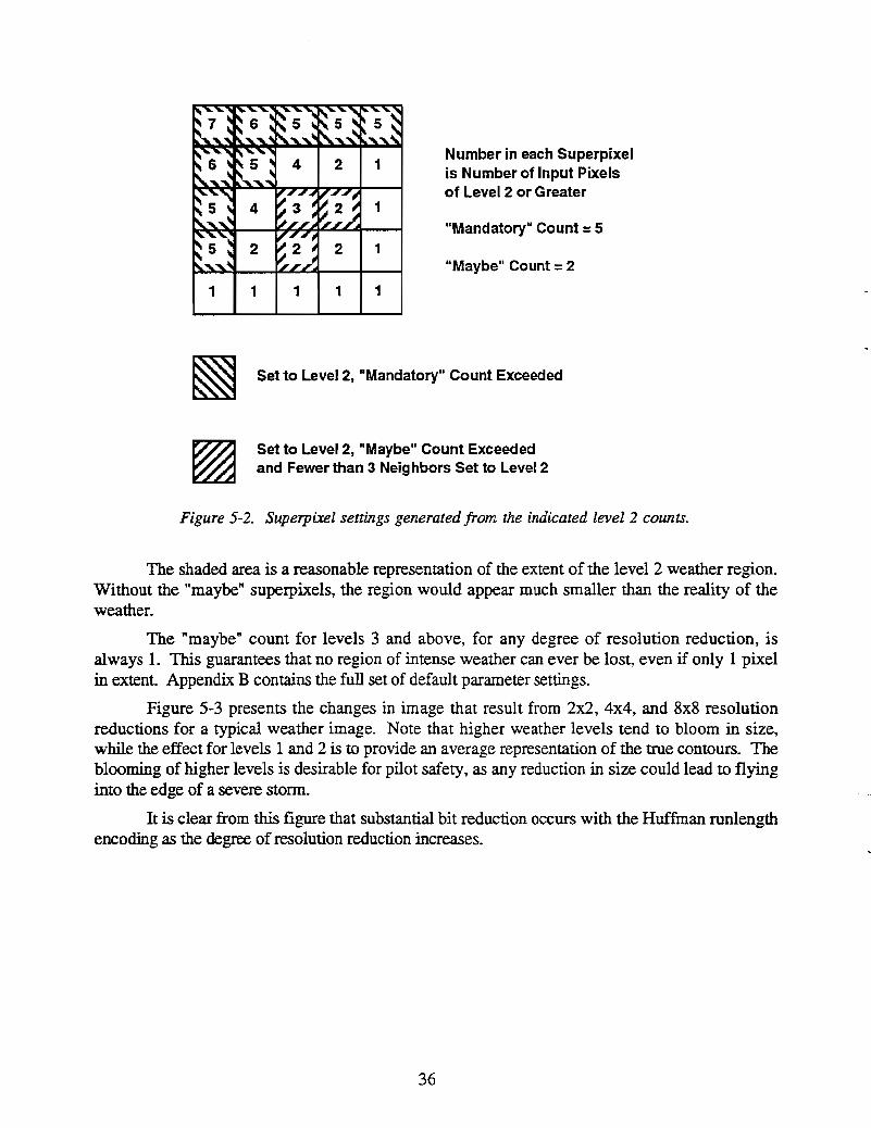
To determine the proper weather level setting of a superpixel, the number of its constituentpixels at or above each level is counted (that is, for example, the level 2 count includes all pixels oflevels 2, 3, 4, 5, and 6). Then, highest level to lowest, each level count is compared to its twothreshold values. If the level count satisfies the "mandatory" threshold, the superpixel componentsby themselves are sufficient to justify setting the superpixel to that weather level.

Otherwise, if the level count satisfies the "maybe" threshold, the superpixel components bythemselves are insufficient to warrant that weather level setting. However, the count is enough thatthe weather region must be represented on the output image. Thus, if not enough of thesuperpixel's neighbors will be set to that weather level to adequately represent the region, thissuperpixel must assume the responsibility by being set to that level.

To determine if such a case exists, the superpixel's 8 horizontal, vertical, and diagonalneighbors are checked to determine how many M of them have already, or will when checked,assume responsibility for representing the weather region. M is determined by comparing theneighbor setting (if already processed) or the neighbor counts (if not yet processed) of each of the8 neighbors. For each neighbor of the former class, M is incremented if its setting is the level inquestion or higher, while for each neighbor of the latter class, M is incremented if its count for thislevel is at least the "mandatory" value. Finally, if the resulting value of M is less than 3, thesuperpixel is set to the level being tested. For this operation, a left-to-right, top-to-bottom row-by­row scan is assumed, so for a superpixel, its W, NW, N, and NE neighbors will have alreadybeen processed, while its E, SE, S, and SW neighbors will not have been processed as yet.

As an example, assume the "mandatory" and "maybe" thresholds for level 2 for a 4x4image are 5 and 2, respectively. This means that any 4x4 superpixel with 5 or more level 2 pixelsout of 16 is automatically set to level 2. Otherwise, any superpixel with a level 2 count between 2and 4 is set to level 2 only when the neighboring superpixels cannot adequately represent theweather region. Applying the above rules, the following superpixel settings are generated from theindicated level 2 counts as seen in Figure 5-2.

35

Number in each Superpixelis Number of Input Pixelsof Level 2 or Greater

"Mandatory" Count =5

"Maybe" Count =2

1 1 1 1 1

Set to Level 2, "Mandatory" Count Exceeded

Set to Level 2, "Maybe" Count Exceededand Fewer than 3 Neighbors Set to Level 2

Figure 5-2. Superpixel settings generated from the indicated level 2 counts.

The shaded area is a reasonable representation of the extent of the level 2 weather region.Without the "maybe" superpixels, the region would appear much smaller than the reality of theweather.

The "maybe" count for levels 3 and above, for any degree of resolution reduction, isalways 1. This guarantees that no region of intense weather can ever be lost, even if only I pixelin extent. Appendix B contains the full set of default parameter settings.

Figure 5-3 presents the changes in image that result from 2x2, 4x4, and 8x8 resolutionreductions for a typical weather image. Note that higher weather levels tend to bloom in size,while the effect for levels 1 and 2 is to provide an average representation of the true contours. Theblooming of higher levels is desirable for pilot safety, as any reduction in size could lead to flyinginto the edge of a severe storm.

It is clear from this figure that substantial bit reduction occurs with the Huffman runlengthencoding as the degree of resolution reduction increases.

36

•....,..'P;.. I .

..

.'7 10;'

r ...Ir' ...

"III-.pt:" .. r/ttiI'Jvt'¥.· "

>

Input Image (tx1) - 22660 Bits Image at 2x2 Resolution - 8927 Bits.

-... • r......

•~. .{. I..: .,

I 'i • •r. r..- .~

•-. I: I• • -• •

Image at 4x4 Resolution - 3245 Bits. Image at 8xB Resolution - 11B2 Bits

Figure 5-3. Mobile Image Encoded at Various Levels of Resolution Reduction.

37

6. SMOOTHING PROCESS

Whenever the Weather-Huffman encoding requires resolution reduction of the input imageto meet the link bit limitation, the decoder must expand the received image back into its fullresolution. Without any other infonnation about the original image to go by, the decoder isreduced to replicating each received superpixel into 4 quadrants of same-level pixels at each step ofthe regeneration. Thus, if a received superpixel were of size 4x4, the decoder would generate 42x2 superpixels, and then 16 1x1 actual pixels, all of the same weather level The result of thisoperation is the generation of an output image with weather regions that are larger and blockier thanthose on the input image.

The Smoothing Process attempts to mitigate this effect by using knowledge of weatherregion shapes to reduce in level some of the pixels at each regeneration step. For example, weatherregions do not often have sharp comers. The Smoothing Process, for reasons of pilot safety, isnot allowed to reduce the extent of weather regions. It is only pennitted to reshape the edges ofregions to drive them closer to expected reality.

6.1 SMOOTHING PROCESS RULES

The rules of the Smoother Process are quite simple. When a superpixel is reproduced, 4comer quadrant pixels are generated. A quadrant may be smoothed down I level only when:

1. All 3 neighboring superpixels of its parent superpixel are of lower weather level thanit is, and

2. Neither the horizontal nor vertical neighbor quadrant in its superpixel meets rule 1.

Figure 6-1 illustrated these rules pictorially, while Figure 6-2 presents sample applicationsof these rules. The effect of rule 1 is to smooth the edges of weather regions by eliminating sharpcomers. Rule 2, on the other hand, precludes the losing of the full extent of the weather regionthat would occur by smoothing away two neighboring regions. The bottom two examples ofFigure 6-2 show how rule 2 prevents compromising the size of the weather region.

A simple cartoon example of smoothing is presented in Figure 6-3, while a full-scaleexample of the application of smoothing when a 4x4 superpixel image is expanded fIrst to 2x2superpixels, and then to Ixi output pixels, is provided by Figure 6-4. It should be clear that theresult is more indicative of the actual underlying weather region than is the unsmoothed post­Huffman picture.

6.2 SMOOTHING PROCESS IMPLEMENTATION

Implementation of the Smoothing Process is simplified via use of the four pre-computedneighbor value lookup tables UL(score), UR(score), LL(score), and LR(score), one for each ofthe four quadrants of the superpixel. The tables are generated by assigning the following values tothe 8 neighbor positions of a superpixel (see Figure 6-1).

39

In Order to Smooth a Corner Quadrant

a) All 3 Neighboring Blocks Must be Lower Level, and

"~~,

b) Neither Neighbor Quadrant May be Smoothable

Figure 6-1. Rules of smoothing process algorithm.

40

Smooth Corner Quadrant

Smooth Diagonal

Don't Lose Extent of Weather

1·,1;; I~J~:;·

< ... I;;)

Can't Smooth Isolated Region

Figure 6-2. Examples of application of smoothing process rules.

41

(a) Original 4x4 Decoding. (b) After Smoothing to 2x2.

(c) Final Smoothing to 1x1.

Figure 6-3. Example of smoothing process algorithm applied to sample weather region.

42

•

.r-

-•

Input Image Image at 4x4 Resolution (No Smoothing)

r

-•

r

-•

Image at4x4 Resolution after Smoothing at 2x2 Image at 4x4 Resolution after FuJI Smoothing (2x2 and Ixt)

Figure 6-4. Effect of Various Leve~s of Smoothing on Output New York Image.

43

UL(s) = 1 for s =

Value Value Value=1 =2 =4

:;,,,,i.;.,""~

Value I~~~ Value~ ....... .~ -'- ~,

=8 = 16

Value Value Value= 32 =64 = 128

For the shaded upper left quadrant of the center superpixel to be smoothable, by the firstrule stated above, the neighbors of values 1, 2, and 8 must all be of lower weather level. But, bythe second rule, either neighbor 4 or 16, and either neighbor 32 or 64, must be of equal or higherweather level. Thus, if a score is generated for the center superpixel by adding the values of allneighbors that are of lower weather level, the set of scores that pennit smoothing of the UL pixelare:

11, 15, 27, 43, 47, 59, 75, 79, 91,

139,143,155,171,175,187,203,207,219

Similar tables are generated for the upper right, lower left, and lower right quadrants.

6.3 SMOOTHING PROCESS OPERATION

When the smoothing algorithm is run, two images are input: the lower resolution image MSalready decoded, and the higher resolution image MR to be created by the Smoothing Process. Forexample, the MS image may be resolution 4x4, in which case the MR image will be 2x2. For eachsuperpixel of image MS, each of the 8 neighboring superpixels are checked to determine thesmoothing score by noting which set of them has lower weather levels.

Then, using the UL table, the upper left quadrant on MR is set equal to the superpixelweather level if UL(score)=O, or instead set one weather level lower if UL(score)=l. Similaractions are taken for the three other quadrants of the superpixel on image MR. To save time,superpixels of weather level 0 are not checked, as all of its quadrants on MR must also becomelevelO.

44

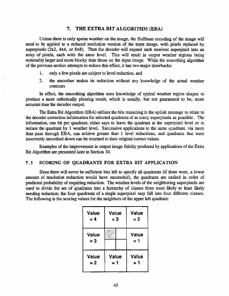
7. THE EXTRA BIT ALGORITHM (EBA)

Unless there is only sparse weather on the image, the Huffman encoding of the image willneed to be applied to a reduced resolution version of the input image, with pixels replaced bysuperpixels (2x2, 4x4, or 8x8). Then the decoder will expand each received superpixel into anarray of pixels, each with the same level. This will result in output weather regions beingnoticeably larger and more blocky than those on the input image. While the smoothing algorithmof the previous section attempts to reduce this effect. it has two major drawbacks:

1. only a few pixels are subject to level reduction, and

2. the smoother makes its reduction without any knowledge of the actual weathercontours

In effect, the smoothing algorithm uses knowledge of typical weather region shapes toproduce a more esthetically pleasing result, which is usually, but not guaranteed to be, moreaccurate than the decoder output.

The Extra Bit Algorithm (EBA) utilizes the bits remaining in the uplink message to relate tothe decoder correction information for selected quadrants of as many superpixels as possible. Theinformation, one bit per quadrant, either says to leave the quadrant at the superpixel level or toreduce the quadrant by 1 weather level. Successive applications to the same quadrant, via morethan pass through EB~ can achieve greater than 1 level reductions, and quadrants that wereincorrectly smoothed down can be returned to their original correct values.

Examples of the improvement in output image fidelity produced by applications of the ExtraBit Algorithm are presented later in Section 10.

7.1 SCORING OF QUADRANTS FOR EXTRA BIT APPLICATION

Since there will never be sufficient bits left to specify all quadrants (if there were, a loweramount of resolution reduction would have succeeded), the quadrants are ranked in order ofpredicted probability of requiring reduction. The weather levels of the neighboring superpixels areused to divide the set of quadrants into a hierarchy of classes from most likely to least likelyneeding reduction; the four quadrants of a single superpixel may fall into four different classes.The following is the scoring values for the neighbors of the upper left quadrant:

Value Value Value=4 =3 =2

Value Ij~~~e:1 Value=3 =1

Value Value Value=2 =1 =1

45

where the number indicated for each neighbor superpixel is added to the score of the upper leftquadrant if that superpixel is at or above the level of the quadrant

Thus, a quadrant totally within a weather region will receive a score of 17 and be the leastlikely to require reduction, while a quadrant of an isolated superpixel will receive a score of O. Thescore values were determined by examining a set of sample images and computing the percent ofthe time a quadrant required reduction when a particular neighbor was below its level; the greaterthe percentage, the higher the assigned score.

7.2 SELECTION OF CLASSES FOR EXTRA BIT APPLICATION

Once all quadrants are scored, the EBA algorithm determines, for each score class, thefraction of its quadrants that require level adjustment Adjustment is required if either:

(a) the quadrant has not been smoothed down, but its correct value is below that of itssuperpixel, or

(b) the quadrant has been incorrectly smoothed down.

For each weather level, a minimum fraction parameter Plevel exists; if a class adjustmentfraction exceed this parameter, it is deemed worth using extra bits for that class.

In theory, the adjustment fraction will be a monotonically decreasing function of score, sothat a "highest worthwhile score" can be found. All scores up to and including this score wouldthen be encoded by EBA, and the rest ignored. In practice, however, the fraction for one score caneasily exceed that of its next lower neighbor. Thus, the algorithm selected to fmd the highest scoreH to use is as follows, where NT and NA are the total number of quadrants of score N and thenumber of quadrants requiring adjustment of score N, respectively:

1. Initialize winning index H= -1.

2. Initialize search index I=-1.

3. Increment J.

4. If IT =0 (no quadrants exist at score J), go to step 3.

5. If ~ ;::: Plevel (score I is worthwhile), set H=I, go to step 3.

6. Set temporary index K =I.

7 . Increment K.

g. Increment JA by KA and IT by KT (combine scores I through K).

IA9. If IT ;::: Plevel , set H=K, J=K, go to step 3.

10. IfK<17, go to step 7.

11. H is the desired score.

Thus, when a score fails the requirements test, and combining that score with successivescores fails to correct the situation, the last successful score is used by EBA Should the fInalvalue of H be -1, no successful score exists, and so no EBA is used for this weather level.

46

Of course, the number of bits remammg in the message may not be sufficient toaccommodate all the quadrants for scores through H. In that case, only a number of quadrantsequal to the number of remaining bits can be specified. The value of Haetual used by EBA will thenby necessity be less than the desired value ofH. In particular, ifB is the number of bits available,Haetua1 is the smallest value such that:

The values specified to the decoder in the encoded message are the score Haetual and thenumber Nmax of quadrants of level Haetual that can be accommodated:

Haetua1-1Nmax = B - LiT

i=l

Ifno bit limitation is encountered, the score Hactual = H and Nmax is unlimited. 5 bits areused to transmit Hactua1, followed by 1 bit to indicate whether Nmax is limited (O=no, l=yes),followed by 9 bits for Nmax if a limitation exists.

7.3 ENCODING ALGORITHM FOR EXTRA BIT APPLICATION

Extra Bit Algorithm (EBA) encoding is performed on one combination of image resolutionand image weather level per call to the routine. The first series of calls is at one level lessresolution reduction than was used for the Weather-Huffman encoding, and occurs after smoothingwas applied to generate the new higher resolution image. The levels are processed in decreasingorder, starting at the image maximum Lmax. If sufficient bits exist for a full pass through EBA tooccur, so that all weather levels are processed, smoothing is again applied to generate the nexthigher resolution image, after which EBA starts again at the highest image level. In the mostextreme case (8x8 Weather-Huffman resolution), three passes can occur through EBA

The encoder employs three images in its processing:

1. Image MS, the superpixel image that exists after Weather-Huffman decoding and anypreviously completed EBA passes are performed.

2. Image MR, the image at the resolution of the routine call, which is one level lessresolution reduction than MS, that exists after the latest smoothing application.

3. Image MA, the input image at the same resolution as image MR.

Image MS is used to determine the neighbor score discussed above for each of the quadrantpixels on image MR, the image to be corrected by EBA. Image MA provides "truth", so that thealgorithm will know which pixels are to have change bit indications sent to the decoder.

The first step in the decoding process is to scan image MS row by row. For eachsuperpixel whose level is at or above the level of the subroutine call, its four quadrants (NW, NE,SW, SE) on image MR are scored and evaluated as to whether a change is required. A change is

47

needed either when the MS pixel is at the same level as the MS superpixel but the true pixel of MAis lower level, or when the MS pixel has been incorrectly smoothed below the MS level

After this scan is complete, the selection of classes for EBA application is determined asdescribed above. Using this selection, and the number of message bits remaining, the values ofHaetual and Nmax are calculated and added to the message, also as described above.

The remaining part of the EBA is the listing in the encoded message of the information bitsthemselves, one for each applicable quadrant on image MR The superpixels of image MS areonce again scanned row by row, and for each quadrant on MR of an applicable superpixel, itsneighbor score is checked (it was computed and saved in the class scoring procedure). If the scoreis less than Hactual, or is equal to Hactnal and is one of the fITst Nmax of that score, a '0' bit isadded to the message if the quadrant should be lower level than the MS superpixel, or a 'I' bit isadded if the quadrant should be at least as high as the MS superpixel

In order for the encoder to process successive EBA calls, it must modify its MR image totrack the actions to be taken by the decoder. Thus whenever a '0' bit is created, if the pixel on MRis above the level of its MS superpixel, the pixel must be set one level below that value. Similarly,whenever a 'I' bit created, and the pixel is of lower weather level than its superpixel, the pixel onMR. must be set to the superpixellevel. These actions ensure that further applications of EBA willrefer to the same image as that used by the decoder.

7.4 DECODING ALGORITHM FOR EXTRA BIT APPLICATION

The EBA decoder is responsible for modifying the weather levels of a set of the superpixelquadrants on the output image that exists after Weather-Huffman decoding. The actions to betaken for the set of quadrants judged worthy of consideration are listed via the message bitsremaining after the Weather-Huffman decoding is completed.

The EBA decoder is called separately for each weather level processed by the encoder. Itmay be called two or three times for the same level if more than one pass through the levels hasoccurred. Of course, successive passes occur at different degrees of resolution reduction.

The EBA decoder uses two weather images. The fITst is the reference superpixel image MSthat exists after Weather-Huffman decoding and any previously completed EBA passes areperformed, while the second is the currently active image MR, of one level less resolutionreduction than MS, that exists after the latest smoothing application. For example, if MS is a 4x4superpixel image, MR. will be a 2x2 image. Each superpixel of MS corresponds to 4 elements ofMR.; these elements (which can be pixels or superpixels) are referred to as the quadrants of the MSsuperpixel.

The scoring classes employed by EBA have been discussed above. The encoderdetermined the highest class to be adjusted by EBA, and if a bit limitation existed, the number ofquadrants at this class that were processed. The decoder's fIrst action is to read these values. ThefITst 5 unread message bits specify the highest class H. IfH=31, this is a signal that no EBA is tooccur at this level, and the decoder simply returns. The next bit indicates whether a limit exits (1)or not (0); if yes, the next 9 bits specify the quadrant count C for score H (if no limit, C is set to.(oo0סס1

48

The remainder of the EBA decoder simply scans image MS row by row. one superpixel ata time. For each superpixel whose level is at least as high as the level of the subroutine call. itsfour quadrants (NW. NE, SW, SE) on image MR are processed. For each, the decoder computesthe neighbor superpixel score, referencing image MS, using the scoring algorithm detailed above.

If the quadrant score S satisfies S < H, or if S = H and the count of such occurrences isone of the first C, a message bit is read to detennine the action to take for the quadrant pixel onimage MR. IT the bit is '0', the quadrant should end up lower than the level of the EBA call; thus ifit is not, it is set to one level less than the calling level. On the other hand. if the bit is '1', thequadrant should end up at least as high as this level If it is lower, due to being incorrectly reducedby the smoothing algorithm. it is returned to the calling level.

49

8. WEATHER-HUFFMAN ALGORITHM ENCODING

This section provides the complete message encoding process utilized by the Weather­Huffman Algorithm. This process incorporates two sub-algorithms:

1. encoding, via the Weather-Huffman runlength algorithm, the highest resolutionversion possible, given a specified data link bit limit, of the original input image

2. using the Extra Bit Algorithm on some or all weather levels to improve the fidelity ofthe output image generated by the runlength decoder

The details of the encoding procedures for the Extra Bit Algorithm have already beenprovided in Section 7, so that infonnation will not be repeated here. Also, many of the details ofthe Weather-Huffman runlength encoding algorithm have been provided in Sections 3 and 4. Onthe other hand. the full set of steps of the Weather-Huffman encoding logic, including when eachof the already discussed routines are utilized, is fully specified below.

8.1 SEQUENCE OF ENCODING METHODS

Unless the input weather image has only very sparse weather, the attempt to losslesslyencode the image via Weather-Huffman runlength encoding will generally exceed the bit limitationimposed on the link. In such cases, a sequence of progressively more reduced resolution andfIltered approaches are applied; the first to meet the bit requirement is used to transmit the imageover the link to the decoder. This section describes in order the sequence of combinationrunlength, smoothing, and extra bit algorithm (EBA) selected for WH. For each method, the sizeof the superpixel (lxI, 2x2, 4x4, or 8x8) used for runlength encoding is listed first. Section 5presented the method employed to construct these superpixels from the original input pixels.

1. IxI encoding

This is the attempt to losslessly encode the input image using the actual pixels. Nosmoothing or extra bits are required.

2. 2x2 encodingThis case attempts to encode the reduced resolution 2x2 image. Theresult is smoothed to lxI, after which any remaining message bits are used by the EBA to correctas many as possible of the incorrect IxI pixels.

3. 4x4 encoding

Experience with sample complex weather images has revealed two facts: most such imagesrequire at least 4x4 resolution reduction to have a chance of meeting typical link bit limitations, andany further resolution reduction to 8x8 produces a decoded image with severe loss of fidelity.Thus, the WH algorithm pursues several subcases in an attempt to encode the image as accuratelyas possible within the 4x4 resolution reduction restriction.

3.a. 4x4 encoding using unfiltered 4x4 image

This case attempts to encode the reduced resolution 4x4 image produced as describedearlier. If successful within the bit limit, the output image is smoothed to 2x2 resolution and theEBA algorithm is applied The lowest level L acted upon by EBA is then noted, and the followingactions taken:

51

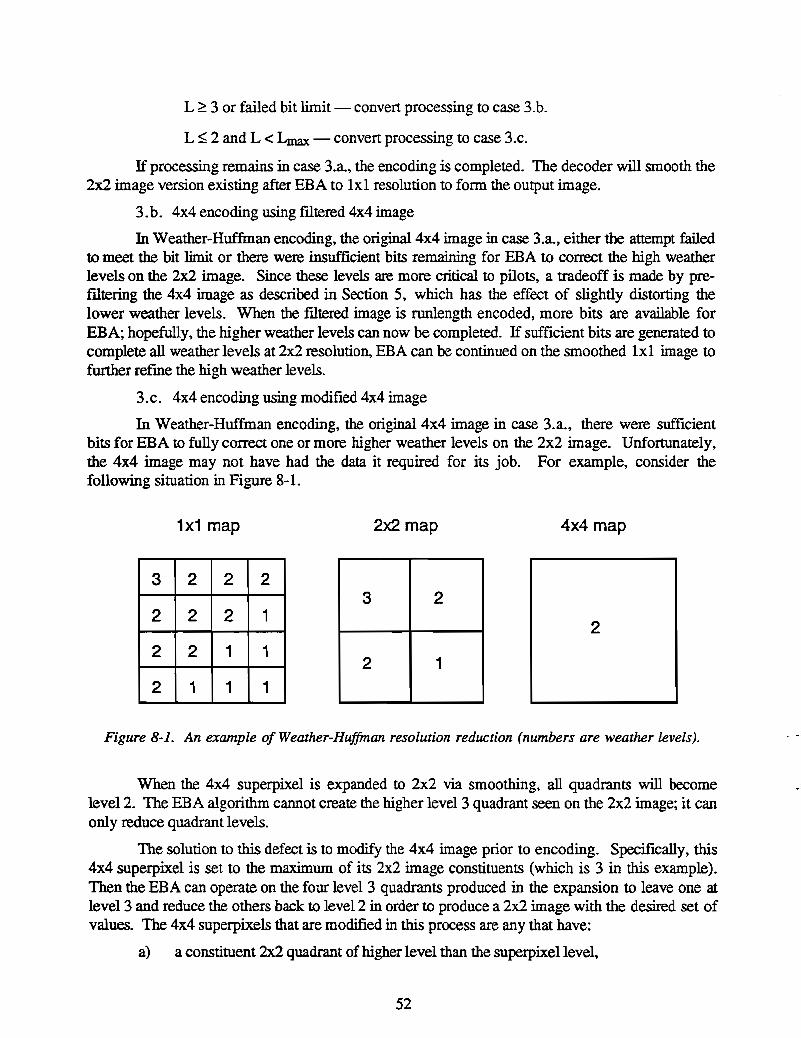
L ~ 3 or failed bit limit - convert processing to case 3.b.

L ::; 2 and L < Lmax - convert processing to case 3.c.

IT processing remains in case 3.a. the encoding is completed. The decoder will smooth the2x2 image version existing after EBA to lxl resolution to form the output image.

3.b. 4x4 encoding using fIltered 4x4 image

In Weather-Huffman encoding. the original4x4 image in case 3.a. either the attempt failedto meet the bit limit or there were insufficient bits remaining for EBA to correct the high weatherlevels on the 2x2 image. Since these levels are more critical to pilots, a tradeoff is made by pre­flltering the 4x4 image as described in Section 5. which has the effect of slightly distorting thelower weather levels. When the flltered image is runlength encoded, more bits are available forEBA; hopefully. the higher weather levels can now be completed. IT sufficient bits are generated tocomplete all weather levels at 2x2 resolution. EBA can be continued on the smoothed lxl image tofurther refme the high weather levels.

3.c. 4x4 encoding using modified 4x4 image

In Weather-Huffman encoding. the original4x4 image in case 3.a.• there were sufficientbits for EBA to fully correct one or more higher weather levels on the 2x2 image. Unfortunately.the 4x4 image may not have had the data it required for its job. For example. consider thefollowing situation in Figure 8-1.

1x1 map

3 2 2 2

2 2 2 1

2 2 1 1

2 1 1 1

2x2 map

3 2

2 1

4x4 map

2

Figure 8-1. An example of Weather-Huffman resolution reduction (numbers are weather levels).

When the 4x4 superpixel is expanded to 2x2 via smoothing, all quadrants will becomelevel2. The EBA algorithm cannot create the higher level 3 quadrant seen on the 2x2 image; it canonly reduce quadrant levels.

The solution to this defect is to modify the 4x4 image prior to encoding. Specifically, this4x4 superpixel is set to the maximum of its 2x2 image constituents (which is 3 in this example).Then the EBA can operate on the four level 3 quadrants produced in the expansion to leave one atlevel 3 and reduce the others back to level 2 in order to produce a 2x2 image with the desired set ofvalues. The 4x4 superpixels that are modified in this process are any that have:

a) a constituent 2x2 quadrant of higher level than the superpixellevel.

52

b) that quadrant is of level L+l or greater, as case 3.a. has already indicated that theseare the levels that will be completed by EBA, and either

cl) this quadrant is of level 3 or higher (severe weather), or

c2) two or more quadrants of the superpixel exist with this level

4. 8x8 encoding

H 4x4 resolution reduction was insufficient to Weather-Huffman encode the image, a finalattempt using 8x8 reduction is made. First, the 8x8 image generated as described in Section 5 isemployed; if this image requires too many bits, the pre-fIltered version of the 8x8 image is created.No tradeoff case as used for 4x4 is employed here, as the lower weather levels have already beenstrongly distorted by the resolution reduction.

4.a. 8x8 encoding using unfIltered 8x8 image

This case attempts to encode the reduced resolution 8x8 image produced as describedearlier. H successful within the bit limit, the output image is smoothed to 4x4 resolution and theEBA algorithm is applied. Ifbits still remain, the new 4x4 image is smoothed to 2x2 and the EBAalgorithm is continued. In the most extreme case, EBA can even be applied to the smoothed Ixiimage.

4.b. 8x8 encoding using filtered 8x8 image

This case is identical to step 4.a. except that the filtered 8x8 image is the starting entity.Again, EBA is applied to each new resolution level in succession until the remaining bits are allused.

5. Increase the message bit limitation

H even 8x8 resolution reduction with filtering fails to produce a image that can be encodedwithin the message bit limitation, this limit must be increased and the encoding process restarted.

8.2 WEATHER-HUFFMAN ENCODING OVERVIEW

The image encoding process of the Weather-Huffman algorithm has four main phases:scanning the image to build the runlength statistics, detennining the codewords to use for eachweather level, encoding the decoding tables corresponding to these sets of codewords, and usingthese codewords to sequentially encode the runs of the image. Scanning can be perfonned byeither a row-by-row raster scan or by a Hilbert scan. As discussed in Section 3, the Hilbert scanwill in general lead to fewer encoding bits and as such has been selected.

Three preparatory operations are required prior to the image encoding itself. The fIrst isgenerating the input image at the resolution reduction level that matches the sequence step beingpursued. The details of the creation of the superpixels for this degree of reduction were providedin Section 5. Next, the linear I-dimensional string of superpixels corresponding to the Hilbertscan of this image must be generated by the code provided in Section 3. During this process, themaximum level superpixel Lmax resident on the image is noted.

Finally, the maximum level superpixel in each 16xl6 image quadrant (corresponding to256 consecutive Hilbert-scanned superpixels) is found and stored in the qmax array. These valuesare encoded in the message so as to be available to the decoder; 3 bits are employed if Lmax>3, 2

53

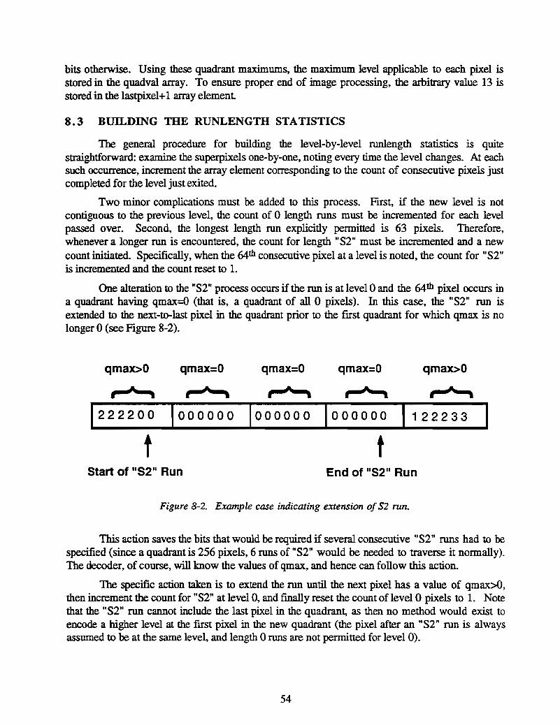
bits otherwise. Using these quadrant maximums, the maximum level applicable to each pixel isstored in the quadval array. To ensure proper end of image processing, the arbitrary value 13 isstored in the lastpixel+1 array element

8.3 BUILDING THE RUNLENGTH STATISTICS

The general procedure for building the level-by-Ievel runlength stallstlcs is quitestraightforward: examine the superpixels one-by-one, noting every time the level changes. At eachsuch occurrence, increment the array element corresponding to the count of consecutive pixels justcompleted for the level just exited.

Two minor complications must be added to this process. First, if the new level is notcontiguous to the previous level, the count of 0 length runs must be incremented for each levelpassed over. Second, the longest length run explicitly permitted is 63 pixels. Therefore,whenever a longer run is encountered, the count for length "S2" must be incremented and a newcount initiated. Specifically, when the 64th consecutive pixel at a level is noted, the count for "S2"is incremented and the count reset to 1.

One alteration to the "S2" process occurs if the run is at level 0 and the 64th pixel occurs ina quadrant having qmax=O (that is, a quadrant of all 0 pixels). In this case, the "S2" run isextended to the next-to-last pixel in the quadrant prior to the fIrst quadrant for which qmax is nolonger 0 (see Figure 8-2).

qmaX>O qmax=O qmax=O qmax=O qrnax>O

, .... , , fA' , , rAt , , rAt , , fA' ,1222200 1000000 1000000 1000000 122233

t tStart of 118211 Run End of 1152" Run

Figure 8-2. Example case indicating extension ofS2 run.

This action saves the bits that would be required if several consecutive "S2" runs had to bespecified (since a quadrant is 256 pixels, 6 runs of "S2" would be needed to traverse it normally).The decoder, of course, will know the values of qmax, and hence can follow this action.

The specific action taken is to extend the run until the next pixel has a value of qmax>O,then increment the count for "S2" at level 0, and fmally reset the count of level 0 pixels to 1. Notethat the "52" run cannot include the last pixel in the quadrant, as then no method would exist toencode a higher level at the fIrst pixel in the new quadrant (the pixel after an "S2" run is alwaysassumed to be at the same level. and length 0 runs are not pennitted for level 0).

54

When the last superpixel of the image is reached, a fmal explicit length run is recorded.This last run cannot be a long "S2" run due to the setting of quadval(lastpixel+1)=13.

The result of this step is the generation of the array Run(L,G), where L ranges fromweather level 0 to level Lmax and G ranges from runlength 0 to runlength 63 and then the 64th

entry is used for runlength "S2". For each level, the longest nonna! non-S2 runlength Rmax isnoted for later use.

8.4 DETERMINING THE CODEWORDS

Once the Run array is determined, for each image level the encoder must detennine thecodewords that will correspond to each non-null runlength. The resulting decoding table must thenbe encoded and added to the message for use by the decoder. The winning codeword set can beone of the three default sets defmed for the level, or be a set tailored specifically for this image.

Before the codewords can be generated for a level, two parameters must be calculated: thelongest explicitly encoded runlength Gmax, and the option 0 to use for encoding "other" longerrunlengths. The methods employed for indicating the incremental runlength of an "other" run werepresented in Section 4. To review, eight options were defmed, five of which always use the samenumber of bits for all runlengths (a different number for each option), while the other three arelong-short options which use two fixed numbers of bits: the smaller for runlengths near Gmax andthe larger for longer runlengths. Depending upon the distribution of "other" runlengths for a level,one option will require the fewest message bits for the encoding of the set of "other" runs.

The first step in detennining the codeword set to use for a level is calculating the number ofbits that would be required for encoding its runs with the default settings. Each default setspecifies the value of Gmax and the codewords for runs of length 0 through Gmax and Sl (the"other" length) and S2 (length exceeding 64). The "other" option to use for runlengths beyondGmax, however, is open. Thus, all eight are tested against the set of "other" runs to select the best,using the procedure detailed in Section 4. The number of bits assigned to each default option isthen the sum of:

1. 3 bits for specifying the "other" option selected

2. the number of bits required by the winning "other" option

3. number of S1 runs x length of S1 codeword

4. number of S2 runs x length of S2 codeword

Gmax5. 1'. (Run(L,j) x length of runlength j codeword)

j=O

The index of the winning default set, and the number of bits it requires for level L runs, is stored.Should there be no runs at level L (winning total =3), the fIrst default set is automatically used forthe level.

Next, the number of bits required for level L by a tailored set of codewords is computed forcomparison. This total would always beat the default case if it weren't for the fact that the bits forthe decoding table now has to be included.

55

With a tailored set, the best value of Gmax to use has to be detennined. Section 4 explainedthe method employed in this search to avoid trying all possible values, which is to skip anyrunlength i for which the number of runs Ri satisfies either:

(a) Ri < Ri+l, or

(b) Ri~l

For any other potential value of Gmax, from -1 (all runs are "other" runs) to Rmax, thenumber of bits required to encode the level is calculated, and the minimum-bit value of Gmax isnoted. For each tested value of Gmax, the steps are as follows:

1. Compute the number of "other" runs:

RmaxRother = L Run(L,j)

j=Gmax+l

2. IfRother> 0, detennine the number of bits required by the winning "other" option asdescribed above for the default cases.

3. Order in decreasing order of number of runs the non-zero runlengths from 0 to Gmaxplus S1 and S2.

4. Calculate the Huffman codeword lengths for each of these runlengths (see Sections 3and 4 for the method).

5. Calculate the number of bits required for the decoding table (see Section 4 for themethod).

The number of bits corresponding to this value of Gmax then becomes the sum of:

1. if Rother > 0, 3 bits for specifying the "other" option selected

2. the number of bits required by the winning "other" option

3. number of S1 runs x length of S1 codeword

4. number of S2 runs x length of S2 codeword

Gmax5. ~ (Run(L,j) x length of runlength j codeword)

j=O

6. number of bits to specify the decoding table

Finally, the bit requirement for the winning default option is compared to the bitrequirement of the tailored codeword set with the optimum value of Gmax. If the tailored set isvictorious, the ensemble of codeword lengths produced by the Huffman algorithm callcorresponding to that Gmax value will be employed in the weather image decoding. The actualcodewords themselves are determined in the next step during the encoding of the decoding table.

To save encoding time, if the bit requirement of the selected alternative, when added tothose of the lower levels already processed, exceeds the message bit limitation, the encodingprocedure is terminated, and the next method of the encoding sequence pursued instead.

56

•

8.S ENCODING THE DECODING TABLE

If a default codeword set is selected, the encoding of the decoder table is trivial:

1. Use 2 bits to encode the number (0-2) of the default set selected.

2. Use 3 bits to encode the winning "other" option.

Then the codewords lengths and codewords themselves of the default ensemble are readfrom storage and transferred to the encoding arrays.

The process is more complicated if a tailored codeword set is selected. In that case, theencoding of the decoder table proceeds as follows:

1. Use 2 bits to encode the number '3', indicating a tailored set of codewords is beingused.

2. Use 3 bits to encode the longest Huffman codeword Hmax being used (maximumlength allowed is 7).

3. Initialize runlength G =-1.

4. Increment G.

5. If G > Gmax, go to step 10.

6. If no runs of length G exist for this level, that is if R(L,G) ::: 0, add a '0' to themessage, and return to step 4.

7. Add a '1' to the message.

8. Determine, as explained in Section 4, the number of bits required to encode the lengthof the codeword Her for runlength G.

9. Encode (Hmax - Ha) using that many bits, and return to step 4.

10. If "other" runs exist, that is if Rother> 0, use 3 bits to encode the winning "other"option.

The last step prior to encoding the image itself is determining the actual codewords for eachrunlength, including S1 and S2. This process, which uses the codeword lengths already knownfrom the call to the Huffman algorithm, was presented in detail in Section 3.

8.6 ENCODING THE IMAGE

The last phase of the encoding process, encoding the image itself, is the simplest. Theimage's superpixels are traversed once again from beginning to end. As each new run terminationis encountered, the codeword (or codewords if an "other" length ron is found), followed by thelevel transition bit (if needed), corresponding to the previous runlength and next level combination,are added to the encoded message. The method of determining the end of a ron is the same asabove, including the special "S2" cases.

If the terminated runlength has an explicit codeword assigned to it (always we for "S2"runs), that codeword is added to the message. Otherwise, the codeword for "SI", the "other"length run, is added to the message. This"S1" codeword must then be followed by the bit

57

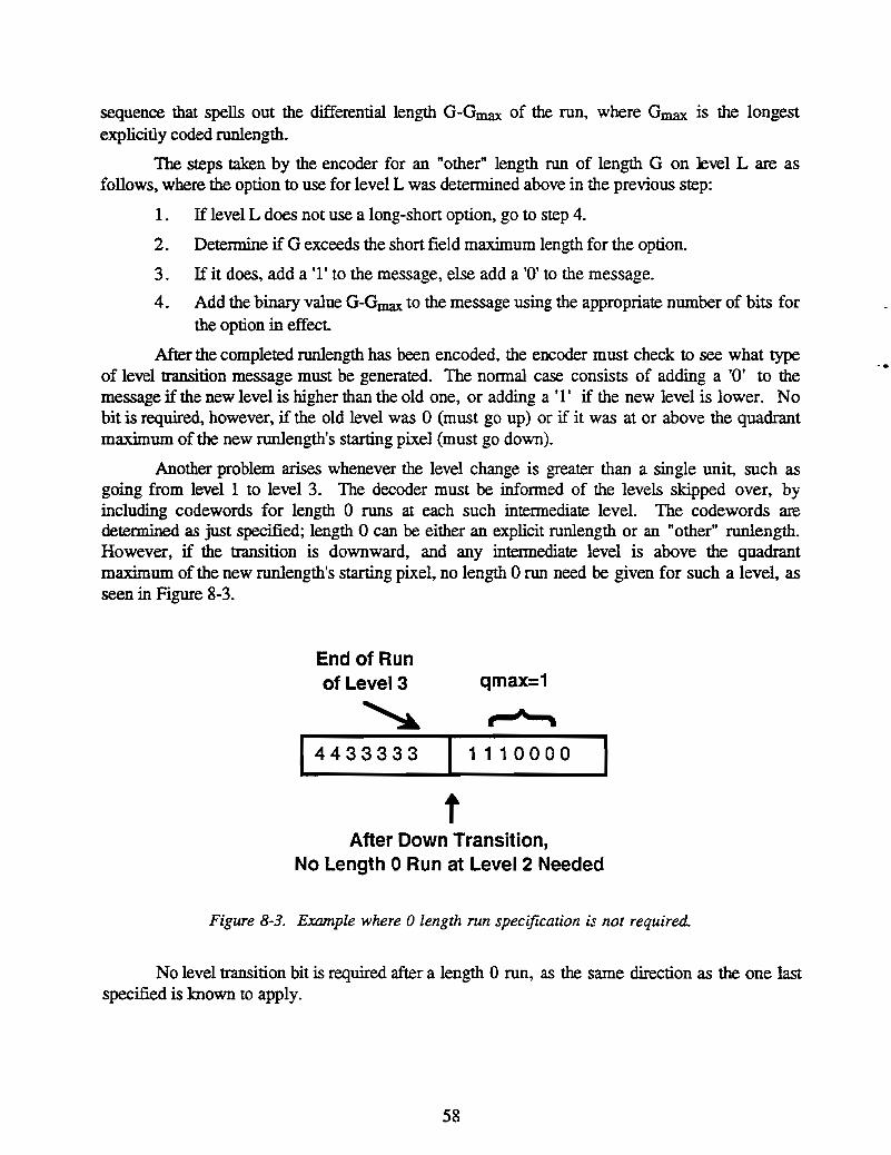
sequence that spells out the differential length G-Gmax of the run, where Gmax is the longestexplicitly coded runlength.

The steps taken by the encoder for an "other" length run of length G on level L are asfollows, where the option to use for level L was determined above in the previous step:

1. If level L does not use a long-short option, go to step 4.

2. Detennine if G exceeds the short field maximum length for the option.

3. If it does, add a '1' to the message, else add a '0' to the message.

4. Add the binary value G-Gmax to the message using the appropriate number of bits forthe option in effect.

Mter the completed runlength has been encoded, the encoder must check to see what typeof level transition message must be generated. The normal case consists of adding a '0' to themessage if the new level is higher than the old one, or adding a'l' if the new level is lower. Nobit is required, however, if the old level was 0 (must go up) or if it was at or above the quadrantmaximum of the new runlength's starting pixel (must go down).

Another problem arises whenever the level change is greater than a single unit. such asgoing from level 1 to level 3. The decoder must be informed of the levels skipped over, byincluding codewords for length 0 runs at each such intermediate level. The codewords aredetermined as just specified; length 0 can be either an explicit runlength or an "other" runlength.However, if the transition is downward, and any intermediate level is above the quadrantmaximum ofthe new runlength's starting pixel, no length 0 run need be given for such a level, asseen in Figure 8-3.

qmax=1End of Runof Level 3

, ,4433333 11110000

tAfter Down Transition,

No Length 0 Run at Level 2 Needed

Figure 8-3. Example where 0 length run specification is not required.

No level transition bit is required after a length 0 run, as the same direction as the one lastspecified is known to apply.

58

•

9. WEATHER-HUFFMAN ALGORITHM DECODING

This section provides the complete message decoding process utilized by the Weather­Huffman Algorithm. This process incorporates three sub-algorithms:

1. decoding the Weather-Huffman runlength-encoded image. which may be resolutionreduced from the original input image

2. applying the Smoothing operation sufficient times to regenerate a image with theoriginal resolution

3. using the Extra Bit Algorithm on some or all weather levels to improve the fidelity ofthe smoothed images

The details of the decoding procedures for the Smoothing and Extra Bit Algorithm havealready been provided in their respective Sections 5 and 6. so that information will not be repeatedhere. The Weather-Huffman decoding logic. on the other hand, is fully specified below.

9.1 DECODER CONTROL LOGIC

Depending upon the degree of input image resolution reduction required to enableapplication of the Weather-Huffman (WH) runlength encoding, and the number of weather levelsthat the Extra Bit Algorithm (EBA) was successful in completing, the decoder will process one ofseven possible cases. The first 3 bits of the message specify the applicable case. The next threebits provide the highest weather level Lmax of the input image. Finally, the next 3 bits specify thelowest weather level LEBA processed by the Extra Bit Algorithm (EBA) on its fmal pass; differentcases are used to represent different numbers of EBA passes. For the last pass. EBA progresses inorder from the highest weather level Lmax to level LEBA; on all prior passes it progresses all theway down to level 1.

The actions taken by the decoder for the 7 possible cases are as follows:

Case I: Ixl WH resolution

The WH decoding will produce directly the Hilbert scanned version of the output image.'This image is then transformed back to the raster scan version which constitutes the fmal image.

Case 2: 2x2 WH resolution

The WH decoding will produce the Hilbert scanned version of the 2x2 resolution outputimage. This image is transformed back to the raster scan version of the 2x2 image, which is thensmoothed to a Ix! resolution image. For each weather level in order, from the highest level Lmaxdown to the level LEBA specified in the message, EBA is applied to correct this image and producethe fmal output image.

Case 3: 4x4 WH resolution with a single 2x2 EBA pass

The WH decoding will produce the Hilbert scanned version of the 4x4 resolution outputimage. This image is transformed back to the raster scan version of the 4x4 image, which is thensmoothed to a 2x2 resolution image. For each weather level in order. from the highest level Lmax

59

down to the level LEBA specified in the message. EBA is applied to correct this image and producea corrected 2x2 image. This image is then smoothed to lxl resolution to generate the [mal outputimage.

Case 4: 4x4 WH resolution with 2x2 and Ixl EBA passes

This case starts the same as case 3. except that all levels of the 2x2 image receive EBAtreatment to produce the corrected 2x2 image, which is then smoothed to generate a Ixl image.For each weather level in order. from the highest level Lmax down to the level LEBA specified inthe message, EBA is applied to correct this image and produce a [mal Ixi output image.

Case 5: 8x8 WH resolution with a single 4x4 EBA pass

The WH decoding will produce the Hilbert scanned version of the 8x8 resolution outputimage. This image is transformed back to the raster scan version of the 8x8 image, which is thensmoothed to a 4x4 resolution image. For each weather level in order, from the highest level !...maxdown to the level LEBA specified in the message. EBA is applied to correct this image and producea corrected 4x4 image. This image is then smoothed to 2x2 resolution, and then further smoothedto Ixl resolution, to generate the [mal output image.

Case 6: 8x8 WH resolution with 4x4 and 2x2 EBA passes

This case starts the same as case 5, except that all levels of the 4x4 image receive EBAtreatment to produce the corrected 4x4 image, which is then smoothed to generate a 2x2 image.For each weather level in order, from the highest level Lmax down to the level LEBA specified inthe message, EBA is applied to correct this image and produce a corrected 2x2 image prior to the[mal smoothing to Ixi resolution.

Case 7: 8x8 WH resolution with 4x4, 2x2. and IxI EBA passes

This case starts the same as case 6, except that all levels of the 2x2 image receive EBAtreatment to produce the corrected 2x2 image, which is then smoothed to generate a IxI image.For each weather level in order, from the highest level Lmax down to the level LEBA specified inthe message, EBA is applied to correct this image and produce the [mal Ix I output image.

9.2 WEATHER-HUFFMAN (WH) DECODING PROCESS

The basic Weather-Huffman decoding process consists of iteratively reading a runlength ata known weather level, followed by determining the direction of transition to the next weatherlevel. In order for the decoder to know the codewords employed by the encoder to specify therunlengths, the message must contain the specifications of the decoding table.

The fIrst step of WH decoding is to check for a maximum weather level of 0; in that case,an empty image is immediately returned. Otherwise. the decoder next reads the weather levelmaximums for each image quadrant These are used to reduce the number of weather transitionsthat require explicit specification: if a run is at the quadrant maximum, a down transition must

60

follow. The number of bits for each quadrant maximum is either 2 or 3, depending upon themaximum weather level for the image (3 bits ifLmax > 3).

After these preliminaries are completed, the process of reading the decoding table anddecoding the weather runs commences.

9.3 DECODING TABLE REPRESENTATION

The fIrst step, and by far the most complex step, of the image decoding operation is theconstruction of the decoding tables for each weather level. As explained in the decoding tableSection 4, numerous "tricks" are employed by the encoder to compress the number of bits requiredto transmit these tables. The job of the decoder is to read the message bits allocated to decodertable specifications, undo these tricks, and produce the array that expresses the decoding tables.

The decoding table array is a 3-dimensional entity of the form:

dec_run(level, #bits, codeword) -> length of run

For example, the entry

dec_run(3, 4, 5) -> 2

says that if you know that the next run consists of level J pixels, and the next ~ message bits to bedecoded are 0101 (binary ~, then the run is of length l.

Most of the entries in the decoder array will set to -1, which is a signal that the entry doesnot correspond to a valid codeword. Since the Huffman code is a prefix code, the followingentries are mandated by the above example:

dec_run(3, 1,0) -> -1,

dec_run(3,2, 1) -> -1, and

dec_run(3, 3, 2) -> -1

since the codewords 0,01, and 010 are all prefixes of the assumed codeword 0101. When thedecoder accesses a decoder array entry of -1, it knows that it must read another message bit in itssearch for the next runlength codeword.

In addition to the decoding array, the decoder must know how to read the actual length ofthe "other" length runs that are signaled by the presence of an SI entry in the decoding array.These lengths are those beyond the longest length explicitly assigned a codeword for the level. Asdetailed in the decoding table theory Section 4, there are 8 possible options for the number of bitsused to encode these runlengths; in 3 of the options, two different lengths, a "long" length and a"short" length, are used. Since the length parameters of each option are fixed, the decoder needonly be told the option number in effect for each level.

9.4 DECODING TABLE CREATION

The actual operation of decoding the message bits that encode a given level's decoding tablecommences with the determination of whether a default table or a tailored table has been selected.For the default cases, the total decoding table generation process is extremely simple:

1. Read T, the value of the next 2 message bits.

61

2. IfT =3, a tailored table specification follows; go to step 5.

3. Copy the default array init{T, i, j, k) into dec_run(i, j, k).

4. Read V, the value of the next 3 message bits;

Set up the parameters for "other" option V for this level

Appendix A lists the default codeword assignments for each level's default tables.

When a tailored table has been constructed for the weather level, the decoder must read thespecification of that table from the message bits. As already described in the encoding Section 8,this specification has been severely compressed to minimize its bit requirement. To review, thebasic form of the specification is a list, in order of runlength, of the number of bits in the codewordassigned to that runlength. The specific runlength ordering is as follows:

51, 52, (0), 1, 2, ....., Rmax

where Rmax is the longest explicitly encoded runlength, Sl is the "other" length designation usedto signal runs between Rmax and 63, S2 signals a run of length greater than 63, and the length of 0is not required for weather levels 0 and Lmax. Once the set of codeword lengths are known, theactual codewords themselves can be determined by the method described in the Huffman theorySection 3.

For each runlength assigned its own explicit codeword, the number of bits required to statethe length of that codeword is a function of the number of lengths still possible. The processconnected with determining this number was detailed in the Huffman table Section 4. That sectionalso explained how a Huffman coding scheme could result in the number of bits actually employedvarying with the codeword length being utilized.

The actual decoding algorithm continuation for determining a level's tailored decoding tablethus becomes:

5. Initialize the sum of the number of codewords used so far to 5 = 0, and the runlengthwhose codeword length is being read to R =51.

6. Read G, the longest codeword length, as the value of the next 3 message bits.

7 . Read the next message bit;

if it is 0, no codeword exists for length R, go to step 13.

8. Use 5 and G to look up D, the range of possible codeword lengths for R, and thenuse D to look up the fewest message bits B that could provide the actual codewordlength for runlength R.

9. Read V, the value of the next B message bits.

10. IfV is not a valid Huffman code for range D, read the next message bit M and set V =2.V +M.

11. Look up the offset F corresponding to V;

the codeword length for R is LR =G - F.

62

12. Increase S by the number of codewords covered by LR;

if S = 128, all explicit lengths have been specified, go to step 14.

13. Set R to the next run1ength in the list;

return to step 7.

14. Using the set of values LR, determine the actual codewords for Sl, S2, and eachexplicit length run and create the decoding array dec_run.

15. If a codeword exists for Sl, the tailored decoding table uses an "other" option;

read V, the value of the next 3 message bits;

set up the parameters for "other" option V for this level.

9.S IMAGE RUNLENGTH DECODING

After the decoding array dec_run has been established, the actual decoding of therunlengths of the Weather-Huffman encoded Hilbert-scanned image can commence. The next 3bits of the message specify the level Ll of the fIrst image superpixel. Each runlength in turn is thenread. The basic idea is to read message bits until a valid codeword is located.

Level transitions are read via one message bit (up or down) after each run except when thechoice is predetermined. In particular, up is assumed after level 0, down is assumed after a run at

the quadrant maximum level, and transition to the new quadrant maximum level is assumed after arun above that level. Multiple level transitions are handled by having a runlength of length 0 foreach skipped over level, after which a transition in the same direction is assumed.

The sequence of steps for detennining each runlength and transition pair is as follows:

1. Initialize last decoded pixel P to 0, level L to Ll.

2, Initialize codeword C to 0, number of codeword bits N to o.3. IfR = dec_run(L, N, C) is ~ 0, the runlength has been found;

go to step 5.

4. Increment N and read the next message bit B;

setC=2~ +B;

return to step 3.

5. If R = SI ("other" length), follow rules of the "other" option in effect for level L todetennine actual R (see below).

6. If R = S2 (run> 63), set R = 63 unless L = 0 and the quadrant max level is 0, inwhich case extend R through the next to last superpixel for which the quadrant max iso(if extended to last one, a change from level 0 at the next superpixel would beimpossible to specify, as no length 0 run at level 0 is pennitted).

7. Set superpixels P+1 through P+R to L.

8. Increase P to P+R.

63

9. IfP = end of image, quit.

10. If level transition is not assumed to be known, read next message bit B;

B=O -> up, B=l -> down.

11. Set new value ofL;

return to step 2.

As described earlier, two types of "other" options exist The fIrst type always employs aflXed number of bits F to specify the actual runlength. When such an option is in effect, the next Fmessage bits are read to produce the value V, and the true runlength R is given by

R=Rmax+V

where Rmax is the longest explicitly encoded runlength for level L.

The second type of option employs two different numbers of bits for runlengthspecification. Thus the next message bit must be read to determine which length to use: the shorterlength (bit ='0') or the longer length (bit = 'I I). Once the length. is known, that many bits areread, and the procedure for computing R is then the same as for the single length case.

64

10. WEATHER-HUFFMAN ALGORITHM RESULTS

This section presents more detailed results (beyond those provided in Section 2) ofapplying the Weather-Huffman Algorithm to various sample weather images. It also highlights theeffectiveness of each part of the algorithm by showing incremental results. Various bit limitationsare also applied to indicate the graceful degradation properties of the algorithm. For ease ofviewing results, all images have been converted to 3-level weather: green for light rain, yellow formoderate rain and turbulence, and red for heavy rain and severe turbulence.

10.1 DEGREES OF RESOLUTION REDUCTION

Filtering provides a significant reduction in encoding bits for a minor change inunage.

A filtered 4x4 image is strongly preferable to an 8x8 image, and thus is worth tryingfirst.

2.

The greater the degree of resolution reduction forced on the algorithm by the bit limitation,the greater the loss of fidelity that results in the encoded image. Figure 10-1 presents, for a sampleimage, the four levels of reduction considered by the Weather-Huffman Algorithm: none (or lxlsuperpixels), 2x2, 4x4, and 8x8. It is clear that as resolution decreases, two significant effectsoccur: the weather regions become blockier, and higher weather level regions bloom in size. Theblooming alternative is to lose small regions of high level weather, which for pilot safety reasons isunacceptable.

The figure also provides information on how the encoder bit requirement decreases withgreater resolution reduction. The ratio for each step is approximately 2.5 : 1, rather than the 4 : 1that might have been expected by just counting pixels to be encoded. The reason for this is two­fold: the decoding table overhead increases in importance as the message decreases in size, and theHuffman efficiency decreases as the number of runs decreases.

The algorithm also allows image fIltering at both the 4x4 and 8x8 resolution steps, in orderto decrease the encoding bit requirement and thus possibly meet the bit limitation without needingfurther resolution reduction. Figure 10-2 indicates the output images, and bit requirements,produced both with and without fIltering for the 4x4 and 8x8 levels. Two results are clear fromthis figure:

1.

10.2 INCREMENTAL RESULTS

The Weather-Huffman Algorithm contains three separate subalgorithms:

1. Weather-Huffman runlength encoding a resolution-reduced version of the inputimage.

2. Smoothing the resolution-reduced output image back to the original resolution.

3. Applying the Extra Bit Algorithm to correct errors introduced by the resolutionreduction.

Figure 10-3 illustrates the effectiveness of each step by presenting the results of skippingsome of the subalgorithms. The upper left picture is the input image. The upper right picture is the

65

output of Weather-Huffman runlength encoding when a 3500 bit limit is imposed. The algorithmwas forced to encode a reduced version of the input with 4x4 superpixels, which required 1962bits. 1be blockiness of this resolution reduction is quite apparent. The lower left picture showsthe effect of employing smoothing on the previous image: the edges of the regions have becomemore realistic, but unfortunately the regions are still as large as before. Finally, the lower rightpicture includes the Extra Bit Algorithm processing, using the bits remaining in the 3SQO-bit limit.It is clear that the red regions have been significantly altered, removing most of the blooming thatresulted from the original resolution reduction. In addition, the shapes of the yellow regions havebeen significantly improved.

10.3 ALGORITHM TRADEOFFS

It is possible to trade off resolution reduction for increased extra bit coding. That is, apossible alternative is 2x2 runlength encoding with no Extra Bit Algorithm versus 4x4 runlengthencoding with 2x2 EBA correction employed in the freed up bits. Figure 10-4 considers thesealternatives. The upper left image is the input image for the example. The upper right imagepresents the result of 2x2 Huffman encoding only, while the lower left image is the output from4x4 Huffman encoding followed by a complete pass of EBA at the 2x2 level.

The first thing to note is that 4x4 with EBA requires significantly fewer bits. This isbecause EBA only attempts to correct the edges of existing regions. Thus, as seen in thecomparison of the images, several more green regions, with superior internal structure, exist in the2x2 image. The red areas, however, are very similar between the images.

A more fair comparison would be to allow EBA to utilize all the bits freed up by going to4x4 resolution. The lower right image presents this result. Comparing it with the 2x2 imageabove it, it is seen that, although the green regions are still inferior, the red regions are significantlymore accurate. This results from the EBA being able to correct the red at the lxl resolution in itssecond pass through the weather levels.

Thus, a real tradeoff exists for operational evaluation: is it better to concentrate on accuracyof higher or lower level weather regions. The resulting opinion could alter the decision currentlyused in the Weather-Huffman algorithm, which is to use the least possible resolution reduction forthe Huffman encoding step. It should be noted, however, that if the tradeoff for a severe weatherimage is between 4x4 reduction versus 8x8 with EBA, the loss of fidelity with 8x8 reductionmakes it the losing alternative.

10.4 VARIATION IN LINK BIT LIMIT

Obviously, the more bits allocated to image encoding, the more faithful will be the outputresult Figures to-Sa and to-Sb illustrate this effect by presenting the output images produced fortwo sample images at three different bit limits: 2300, 3500, and 4700.

As the bit limit is increased, the shape and sizes of the various weather regions increase inaccuracy. Note that because of the priority scheme employed by the Extra Bit Algorithm, higherweather regions are better preserved than lower ones with lower bit limits. Put another way, thedegradation of the output images as the bit limit is tightened is moderate for the most criticalweather infonnation. In fact, both of the 23OQ-bit images are probably acceptable for strategicflying.

66

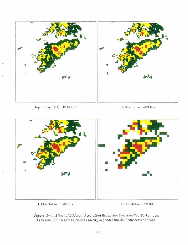
r

-•

Input Image (Ix1) - 12651 Bits

4x4 Resolution - 1962 Bits

J

-••

2x2 Resolution - 4974 Bits

...8x8 Resolution - 731 Bits

Figure 10-1. Effect of Different Resolution Reduction Levels on New York Image.As Resolution Decreases, Image Fidelity Degrades but Bit Requirement Drops.

6

r

-•

-••

.......

4x4 Resolution - No Filtering - 1962 Bits

• ••

8x8 Resolution - No Filtering - 731 Bits

r

-

-...,.

4:<4 Resolution - With Filtering - 1507 Bits

8x8 Resolution - With Filtering - 538 Bits

...

Figure 10-2. Effect of Runlength Filtering at Lower Resolut'i.on Levels on New York Image.Fidelity Undergoes Minor Change while Bil Requirement D7'OpS Significantly.

68

•

•

Input Image

•

•

Smoothing Process Included - Still 1962 Bits

Huffman Runlength Encoding Only (4x4) - 1962 Bits

•

Extra Bit Algorithm Applied to 3500 Bit Limit

Figure 10-3. Output New York Image Existing after Each Incremental Step of the WH Algorithm.

69

'.

..

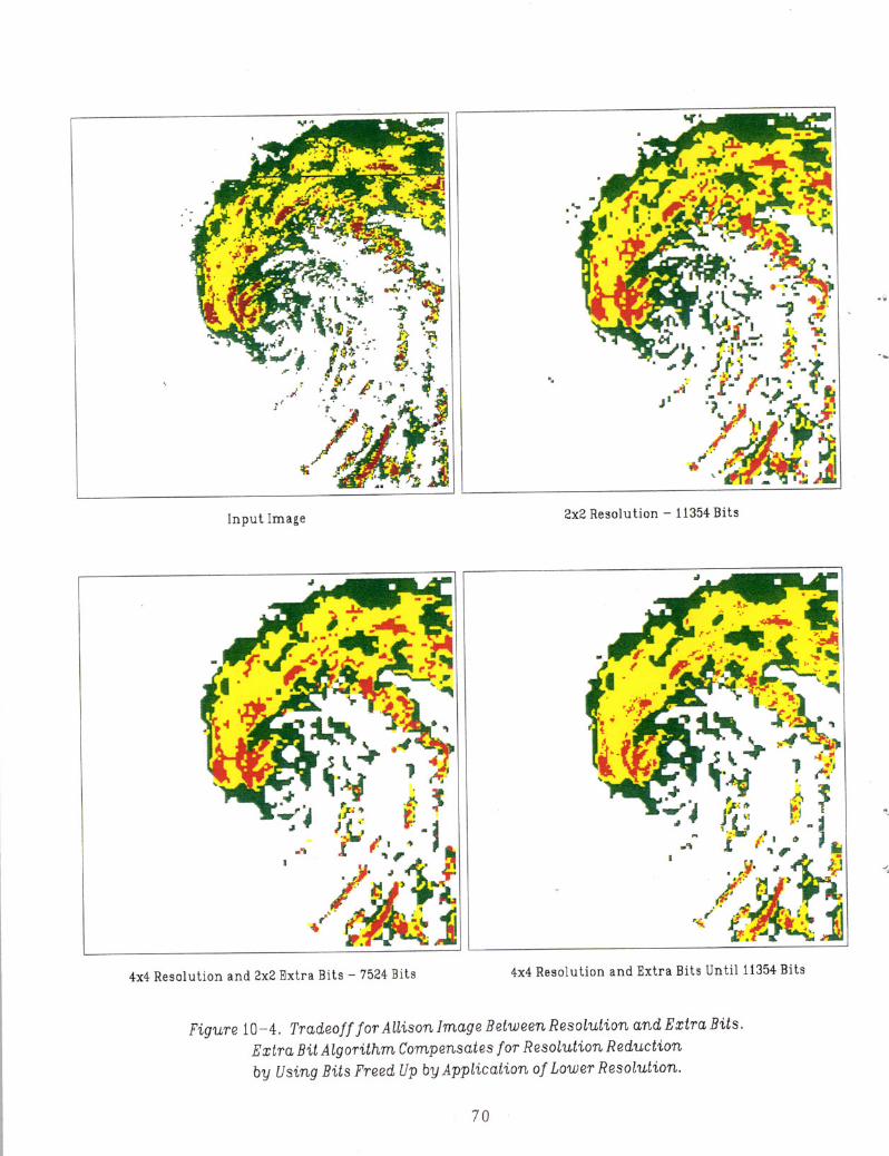
Input Image

4x4- Resolution and 2x2 Extra Bits - 7524 Bits

2x2 Resolution - 11354 Bits

4-x4 Resolution and Extra Bits Until 11354 Bits

Figure 10-4. Tradeoff for Allison Image Between Resolution and Extra Bits.Extra Bit Algorithm Compensates for Resolution Reductionby Using Bits Freed Up by Application of Lower Resolution.

70

•

, 4- :i4" """i~~,~

j,~.;. )f ,. ~ .• j -I

, . i;l-r 4 f~.

·r

Tj:. \.

\

•

-..

•

,.. . .

;~l~~. .~.. .. I... ,• •... ,

•

-

Input Image

•

Output Image with 2300 Bit Limit

-..• • • •

.,., r .•

., ,.: ..• ; ~04 .. f'» ..

t' ~ • ''''", •W ~:... r. .:-.,... ~;.-

..

~::.

.j.~:~-... ~ ~.

•

•

-• •• •

,. .

,.

Output Image with 3500 Bit Limit Output Image with 4700 Bit Limit

Figure 10-5a. Output Mobile Image as a Funct'i..on of Datalink Bit Limit.

71

Input Image

Output Image with 3500 Bit Limit

Output Image with 2300 Bit Limit

Output Image with 4700 Bit Limit

Figure 10-5b. Output Allison Image as a Function of Datalink Bit Limit.

72

APPENDIX ADEFAULT HUFFMAN ENCODING ENSEMBLES

This Appendix presents, for each image level, the 3 options available for default Huffmancodeword ensembles. For each option, the codeword bitlength L and the actual codewordassignment are listed for each applicable runlength. The special "runlengths" Sl and S2 are alsoincluded, where as described in the report:

S1 indicates an "other" length run, length> LmaxS2 indicates a long run, length> 63

where Lmax, also listed for each option, is the longest runlength assigned its own codeword.

73

Level 0

Option 0 Option 1 Option 2

Lmax =7 Lmax =S2 Lmax =8

Runlength L Code L Code L Code

S1 4 1000 1 0 2 01

S2 1 0 1 1 2 00

1 4 1001 4 1000

2 4 1010 4 1001

3 4 1011 4 1010

4 4 1100 4 1011

5 4 1101 4 1100

6 4 1110 4 1101

7 4 1111 4 1110

8 4 1111

Level 1 and 2

Option 0 Option 1 Option 2

Lmax=5 Lmax =S2 Lmax =7

Runlength L Code L Code L Code

S1 3 000 1 0 2 00

S2 3 001 1 1 2 01

0 3 010 4 1000

1 3 011 4 1001

2 3 100 4 1010

3 3 101 4 1011

4 3 110 4 1100

5 3 111 4 1101

6 4 1110

7 4 1111

74

Levels 3, 4, 5, and 6

Option 0 Option 1 Option 2

lmax=2 Lrnax =2 Lmax=4

Runlength L Code L Code L Code

51 3 110 1 0 2 00

52 3 111 3 111 3 010

0 2 00 3 100 3 011

1 2 01 3 101 3 100

2 2 10 3 110 3 101

3 3 110

4 3 111

Level?

Option 0 Option 1 Option 2

Lmax =2 Lmax =2 Lmax =4

Runlength L Code L Code L Code

51 3 110 1 0 2 00

52 3 111 3 111 3 010

1 2 00 3 100 3 011

2 2 01 3 101 3 100

3 2 10 3 110 3 101

4 3 110

5 3 111

Note that, for levels 0 and 7, no codeword need be assigned to a runlength of O. Arunlength of 0 is used to cover multi-level weather changes through the given level For example,a change from level 3 to level 1 requires a codeword for a length 0 run at level 2. Clearly, nochange "through" level 0 or 7 is possible. For an actual image, no codeword for length 0 would berequired for the highest weather level existing on that image. Thus, whenever the highest imagelevel is 3 or greater, the default ensemble of level 7 is used for that highest level.

75

APPENDIXBWEATHER-HUFFMAN (WH) PERFORMANCE-TRADEOFF PARAMETERS

This Appendix lists and defmes each of the peIfonnance-tradeoff parameters currentlyexisting in the WH algorithm software. It also lists the current default settings of each parameter,and discusses the peIformance effects of changing to other values.

Image Bit Limit (maxbits) Default = 3500

This parameter is the maximum number of bits that can be used to encode the weatherimage. Changes in the setting will increase or decrease the distortion produced in the imagerepresentation output to the pilot

Level Renumbering (remapp) Default = 0

This parameter specifies whether the standard weather level numbering scheme should bemaintained on the input image, or whether some of the levels should be grouped. The meanings ofthe possible values are:

o= no renumbering of weather levels

1 =renumber the weather levels

the user must enter in order the new numbers for levels 1 through 6.

The remapping feature is useful when fewer than 6 levels of weather are desired on theoutput display. For example, a 3 level display - light rain, heavy rain, storms - would beproduced by entering 1 followed by the 6 values 1,2,3,3,3,3, which combines together all pixelsof levels 3 through 6.

Minimum Level Count for 8x8 (wt8g) Default =32,20,6,1,1,1

These parameters specify, for each level I through 6, the minimum count of pixels at orabove that level that require the 8x8 resolution reduced superpixel to be set to that level. Forexample, if 20 or more of the 64 pixels in the superpixel are of level 2 or above, and if none of thehigher level thresholds are satisfied (i.e., there are fewer than 6 at or above level 3, and none at

levels 4, 5, or 6), the superpixel is set to level 2. If the values are decreased, weather regions willbe "averaged up" in size, and more weather "spots" will be maintained on the output image; if theyare increased, the larger regions will be more faithfully represented as more bits are freed up forencoding them.

Minimum Level Count for 4x4 (wt4g) Default = 8,5,2,1,1,1

The analog for 4x4 superpixels.

Minimum Level Count for 2x2 (wt2g) Default =2,1,1,1,1,1

The analog for 2x2 superpixels.

Provisional Level Count for 8x8 (wt8) Default = 12,6,1,1,1,1

These parameters specify, for each level 1 through 6, the provisional count of pixels at orabove that level that require the 8x8 resolution reduced superpixel to be set to that level if notenough neighboring superpixels are available to adequately represent the weather region. Forexample, if6 OT more of the 64 pixels in the superpixel are of level 2 or above, and if none of the

77

higher level thresholds are satisfied (i.e., there are none at levels 3, 4, 5, or 6), the superpixel is setto level 2 if less than two neighboring superpixels are set to level 2. This parameter works as aprotection against the previous parameter (wt2g) causing the loss of a significant weather region.If the values are decreased, weather regions will be further "averaged up" in size, and additionalweather "spots" will be maintained on the output image; if they are increased, the larger regionswill be more faithfully represented as more bits are freed up for encoding them.

Proyisional Level Count for 4x4 (wt4) Default =4,2,1,1,1,1

The analog for 4x4 superpixels.

Provisional Level Count for 2x2 (wt2) Default =1,1,1,1,1,1

The analog for 2x2 superpixels.

Extra Bit Usefulness Multiplier (mult) Default = 4,5,7,7,7,7

This parameter specifies, for each weather level, the fraction of the quadrants in an extra bitclass that must require level adjustment for the class to be encoded by the Extra Bit Algorithm. Forexample, for level 2, a given extra bit class must satisfy:

mu1t[2] * (adjusted quadrants) ~ (total quadrants)

for the class to be encoded. By reducing the value for a level, that level will be more accuratelyrepresented on the output image at the expense of lower levels. (Due to the possibility of multipleextra bit passes, reducing the value for a level can in some cases degrade that level as well).

78

J

REFERENCES

[1] Lelewer. D. E., and D. S. Hirschberg, "Data Compression," ACM Computing Surveys. 19,

3 (September 1987): 261-296.

[2] Gertz, J. L., and R. D. Grappel, "Encoding Approaches for Data Link Transmission of

Weather Graphics," Lexington, MA, M.LT. Lincoln Laboratory Project Report ATC-205,

10 December 1993.

[3] Huffman D. A., "A method for the construction of minimum-redundancy codes,"

Proceedings IRE, 40,9 (September 1952): 1098-110l.

[4] Gertz, J. L., "The Polygon-Ellipse Method of Data Compression of Weather Maps,"

Lexington, MA, M.lT. Lincoln Laboratory Project Report ATC-213, 28 March 1994.

79