The Wealth Elasticity of Political Contributions by the...

0

The Wealth Elasticity of Political Contributions by the Forbes 400

Adam Bonica * Howard Rosenthal**

Stanford University New York University

Abstract: Inequality in campaign contributions in the American plutocracy has grown

hand in hand with the growth in economic inequality. We report on the campaign

contributions of the Forbes 400 wealthiest individuals from 1983 to 2012. We find that

the wealth elasticity of individual contributions is around 1.0 without statistical controls

but remains around 0.6 even with fixed effects for individuals and election cycles. The

results suggest that the inequality in campaign contributions is largely driven by the

increase in economic inequality. The sensitivity of contributions to individual wealth

mainly benefits Republicans. In contrast, turnover in membership in the 400 has favored

the Democrats.

* Department of Political Science, Stanford University, 307 Encina Hall West, Stanford,

CA 94305, [email protected].

** Wilf Family Department of Politics, New York University, 2nd Floor, 19 W. 4th Street,

New York, NY 10012, [email protected]

1

The Forbes 400 series of the wealth of the 400 wealthiest Americans, published

annually since 1982, allows us to match wealth with individual campaign contributions in

federal elections. The direct empirical motivation of the paper is to examine whether the

contributions of the super wealthy correlate with variations in their individual wealth.

We have constructed a (unbalanced) panel of wealth and contributions data for 1982-

2012.

In a larger context, however, it is important to ask how political inequality, as

measured by inequality in campaign contributions, relates to inequality in wealth.

Individual contributions are important and have been larger, when aggregated, then

contributions by PACs (political action committees) and other organizations (Bonica et

al., 2013). The number of campaign contributors, computed from itemized reports to the

Federal Election Commission and the Internal Revenue Service has increased rapidly in

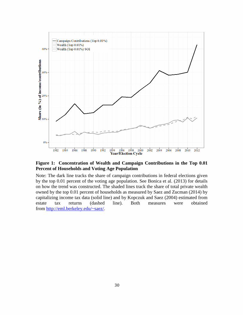
recent years, passing 3,000,000 in the 2012 election cycle. Despite the increase in mass

participation, the share of campaign contributions provided by the top 0.01% of

contributors in the voting age population has risen sharply (Bonica et al., 2013) and is far

greater than the share of income captured by the top 0.01% of the income distribution

(Piketty and Saez, 2003) or the share of wealth captured by the top 0.01% of the wealth

distribution (Saez and Zucman 2014, Kopczuk and Saez 2004 ), as seen in Figure 1. Even

within the Forbes 400, contributions have become more concentrated.

From the 400 list, we have measurements not of income but of wealth.

Membership on the list evolves rapidly. Nevertheless, the observation that the aggregate

wealth of the 400, inflation adjusted to 2014 dollars, rose from $0.2 trillion in 1982 to

$2.2 trillion in 2014 is striking. We examine whether this rising economic inequality in

wealth has been accompanied by rising political inequality in campaign contributions

both between the 400 and the general population and within the 400.

To summarize, we need to look for empirical results on individual contributions

that are consistent with the observation that contributions have become increasingly

unequal despite the fact that increasing multitudes of citizens are throwing chump change

in the Trevi fountains of American politics. That is, political inequality has grown in spite

of the increase in mass participation.

2

I. Analytical Setup

We begin with a simple setup to suggest the channels by which political

inequality can grow within the framework of our empirical work. We consider a world

with two agents {POOR, RICH}. The wealth levels are 𝑊𝑃𝑂𝑂𝑅 < 𝑊𝑅𝐼𝐶𝐻 . We measure

wealth inequality as the proportion of wealth held by the RICH agent and political

inequality as the proportion of contributions made by the RICH agent. [As an aside, we

note that empirical evidence shows that the RICH agent is more likely to vote than the

POOR one (Bonica et al., 2013)]

Our basic empirical specification is log-linear:

ln(𝐶) = ln (𝛼) + 𝛽 ln(𝑊) 𝑜𝑟 𝐶 = 𝛼𝑊𝛽

The equation presumes that wealth is exogenous to contributions. More on this point in

our concluding remarks.

We define wealth inequality as 𝐼𝑊 = 𝑊𝑅𝐼𝐶𝐻/(𝑊𝑅𝐼𝐶𝐻 + 𝑊𝑃𝑂𝑂𝑅) and political or

contribution inequality as 𝐼𝐶 = 𝐶𝑅𝐼𝐶𝐻/(𝐶𝑅𝐼𝐶𝐻 + 𝐶𝑃𝑂𝑂𝑅) . Observe that if POOR and

RICH share common parameters α and 𝛽, 𝛽 determines whether contribution inequality is

more than wealth inequality. This can occur only if 𝛽 > 1 , when contribution is a

superior good with respect to wealth. In a simple unbalanced panel regression of 𝐶 on W,

𝛽 is indeed estimated to be greater than 1. On the other hand, with fixed effects, 𝛽 is less

than 1.

So how might political inequality between agents RICH and POOR grow?

Political inequality will indeed grow as wealth inequality grows, but 𝛽>1 is still required

for political inequality to be greater than wealth inequality.

Political inequality will exceed wealth inequality only if RICH and POOR have

different parameter values 𝛼POOR , 𝛼RICH , 𝛽POOR , 𝛽RICH . A necessary condition for

political inequality to exceed wealth inequality is either 𝛼POOR < 𝛼RICH or 𝛽POOR <

𝛽RICH. When parameter values are sufficiently distinct, political inequality can exceed

wealth inequality. Parameter values can change over time as the identity of the agents

turns over. Bill Gates, who has topped the 400 for years, was not in the 400 during the

early 1980s.

3

While we have no way to measure parameter values at the individual level for

those not in the 400, we do have the ability to use the data to discover trends that would

be likely to produce increased political inequality. (We also examine the relationship

between wealth and campaign contributions at the level of census-tracts.)

First, for each member of the 400 we have aggregated contributions over the two-

year election cycles of American politics. We estimate cycle fixed effects. These are

important to control for the fact that contributions tend to be more in presidential than in

midterm cycles. Cycle fixed effects also control for both the effect of changes in

campaign finance law and changes in interest in politics perhaps driven by contributing

becoming a display tournament for the wealthy. An increasing sequence of cycle fixed

effects would cause contributions to grow, for a fixed value of β, faster than indicated by

the increases in individual wealth.

Second, there are individual fixed effects, which are important given substantial

heterogeneity in contributions across individuals. These fixed effects may, even after

cycle fixed effects, have a temporal pattern. As membership of the 400 has turned over, it

has become increasingly male dominated 1

Third, temporal variation in 𝛽 could be explored with the same motivation that

suggests looking at cycle and individual fixed effects.

and is likely to reflect more new

entrepreneurial wealth as against inherited wealth (Edlund and Kopczuk, 2009). Again, if

individual fixed effects have grown in time, the contributions of the wealthy would grow

faster than indicated by the increases in individual wealth.

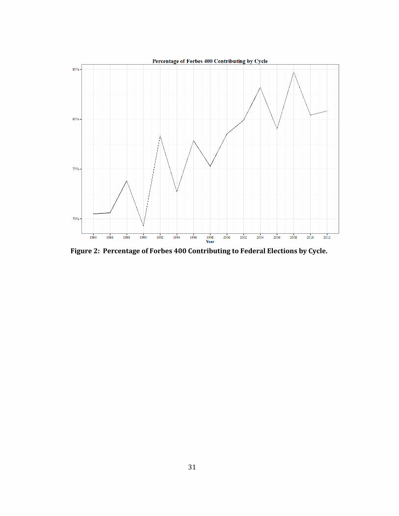
Finally, our estimation is tobit. Tobit posits a wealth threshold below which the

individual fails to contribute. The tobit is motivated by the observation that a substantial

number of 400 members make no contributions. Figure 2 shows that only 72%

contributed in 1984 but that 81% did in 2012.

In section II, we provide an overview of important patterns in the membership of the

400 and in their contributions. In section III, we describe the data. Subsequently, in

section IV we present basic estimation results and do robustness checks. One check

1 The percentage of females in the 400 decreased from 20.2% in 1983 to 12.5% in 2012.

4

includes data on contributions when the individual is not a member of the 400. A second

varies the time period of the analysis, and a third examines panel bias. Section V

validates our results on wealth by using census tract data. The census data also extends

the analysis to income. In section VI we breakdown contribution by whether it is directed

to Republicans or Democrats and by the estimated political ideology of the donor. In

section VII we investigate whether increases in individual wealth relate to partisan

preferences. The two final sections provide discussion and a conclusion.

II. The Politics of Wealth Concentration

Many have considered the connection between politics and inequality. Here we

provide background on relevant trends for the 400.

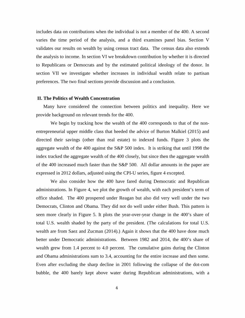
We begin by tracking how the wealth of the 400 corresponds to that of the non-

entrepreneurial upper middle class that heeded the advice of Burton Malkiel (2015) and

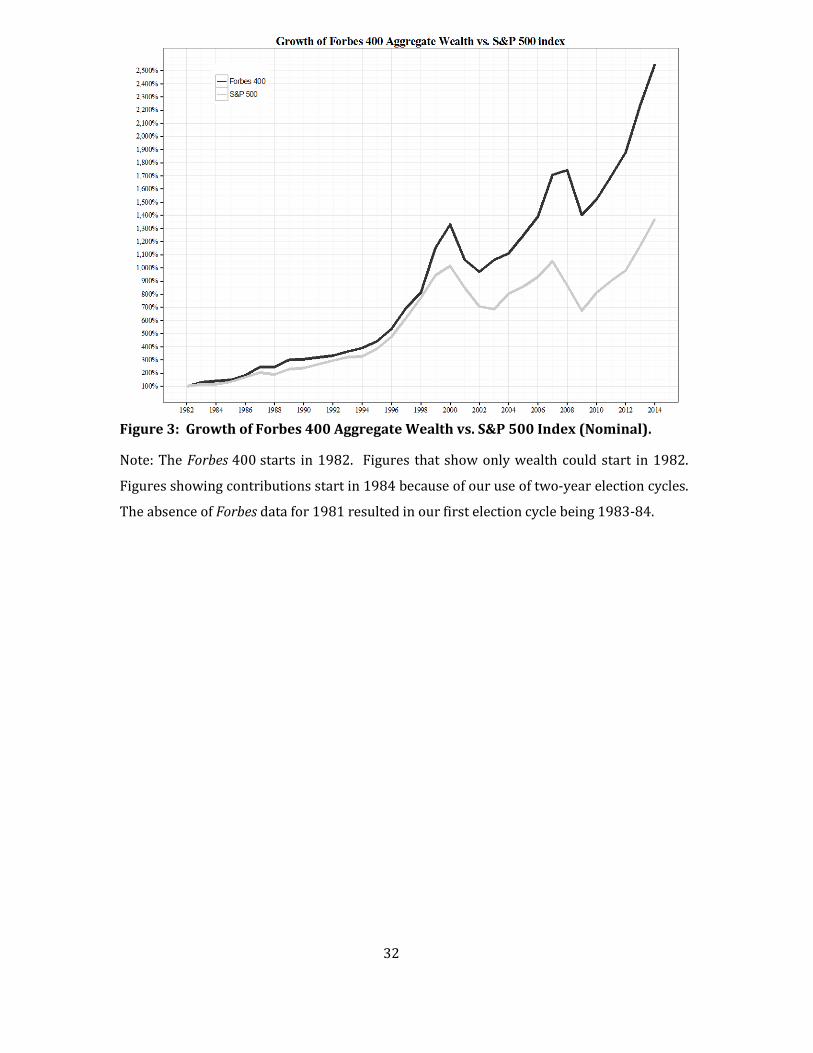
directed their savings (other than real estate) to indexed funds. Figure 3 plots the

aggregate wealth of the 400 against the S&P 500 index. It is striking that until 1998 the

index tracked the aggregate wealth of the 400 closely, but since then the aggregate wealth

of the 400 increased much faster than the S&P 500. All dollar amounts in the paper are

expressed in 2012 dollars, adjusted using the CPI-U series, figure 4 excepted.

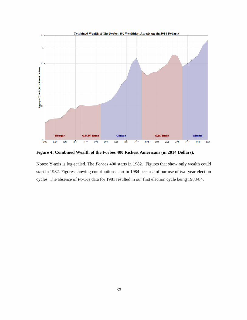
We also consider how the 400 have fared during Democratic and Republican

administrations. In Figure 4, we plot the growth of wealth, with each president’s term of

office shaded. The 400 prospered under Reagan but also did very well under the two

Democrats, Clinton and Obama. They did not do well under either Bush. This pattern is

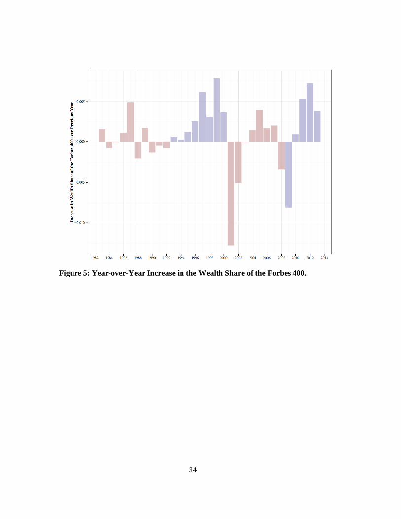
seen more clearly in Figure 5. It plots the year-over-year change in the 400’s share of

total U.S. wealth shaded by the party of the president. (The calculations for total U.S.

wealth are from Saez and Zucman (2014).) Again it shows that the 400 have done much

better under Democratic administrations. Between 1982 and 2014, the 400’s share of

wealth grew from 1.4 percent to 4.0 percent. The cumulative gains during the Clinton

and Obama administrations sum to 3.4, accounting for the entire increase and then some.

Even after excluding the sharp decline in 2001 following the collapse of the dot-com

bubble, the 400 barely kept above water during Republican administrations, with a

5

cumulative gain of just 0.4 percent. The results are similar when using the top 0.00025%

households (data from Saez and Zucman, 2014) in place of the top 400.

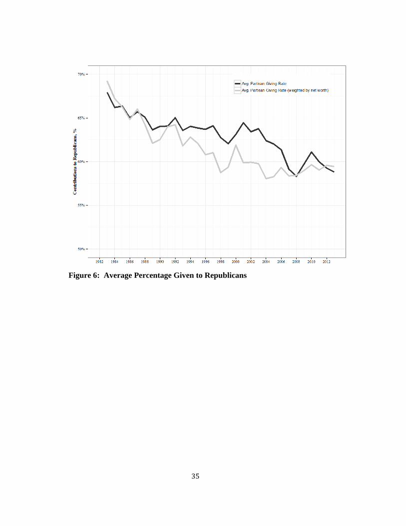
Also of interest are changes in the political orientation of the 400. For each

individual, we construct a measure of partisan giving by calculating the share of major

party contributions given to Republicans. Figure 6 plots two trend lines for the average

percentage contributed to Republicans, one with individuals weighted equally and

another with individuals weighted by the Forbes estimate of wealth. The 400 have

trended steadily to the left even as their fortunes swelled.

This trend is all the more remarkable given that the composition of the 400 has

been impervious to the changing demographics of labor markets and other areas of

society. The 400 in 2012 was 89% percent male, 66% over the age of 60, and

overwhelmingly white—all groups that voted disproportionately for Mitt Romney in

2012—but the 400 are less Republican than what one might expect based on this

demographic profile. This is perhaps made less surprising when taking into consideration

how the 400 have fared during Democratic administrations. It is also the case that

changes in partisanship could well reflect changes from a manufacturing and extraction

economy to a technology and information economy—Silicon Valley and Hollywood are

generous to Democrats.

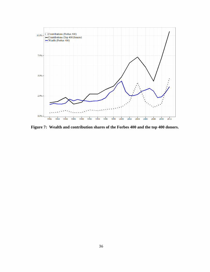
Over time, the share of all individual contributions made by the 400 has

increased. This marker of increased political inequality is shown in Figure 7. In the 2004

and 2012 election cycles, the share of contributions increased to the point where the 400

had a greater share of contributions than their share of wealth. The figure also shows the

contribution share of the top 400 donors in each election cycle. Clearly, the 400 are far

from representing all the largest contributors; the result shows that there is a high degree

of heterogeneity in individual contributions.

In the most recent presidential election cycle, 2011-12, the Forbes 400 were hefty

contributors but were still far from dominating the set of large contributors. Of the top

400 donors in the 2011-12 election cycle, only 64 were also on the Forbes 400; another

21 had appeared on the list in the past. Many of the largest donors are from the class of

not-quite-so-fabulously wealthy individuals with fortunes measured in the hundreds of

millions rather than billions. Fred Eychaner, whose net worth was estimated at $500

6

million in 2005 (about two-thirds of the amount required to make it onto the list that

year), has been among the top ten among Democratic donors donating a total of $21.6

million during the 2004-2012 election cycles. Over the same period, Bob J. Perry, whose

estate was estimated at $650 million at the time of his death in 2013, gave an average of

$13.5 million per election cycle in support of conservative causes, for a total of $67.5

million, making him second only to Forbes 400 member Sheldon Adelson in total

donations.2

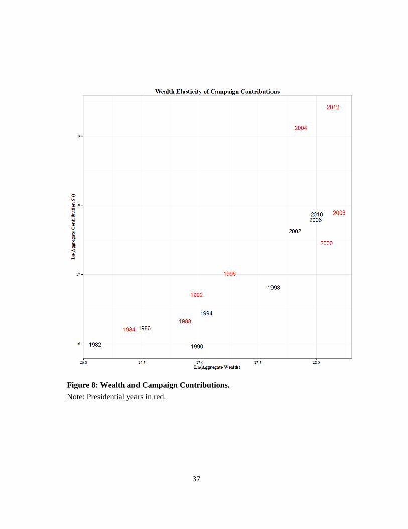
Figure 8 plots logged total contributions of 400 members in each election cycle

against logged wealth. Observe that the figure shows very large contributions in two

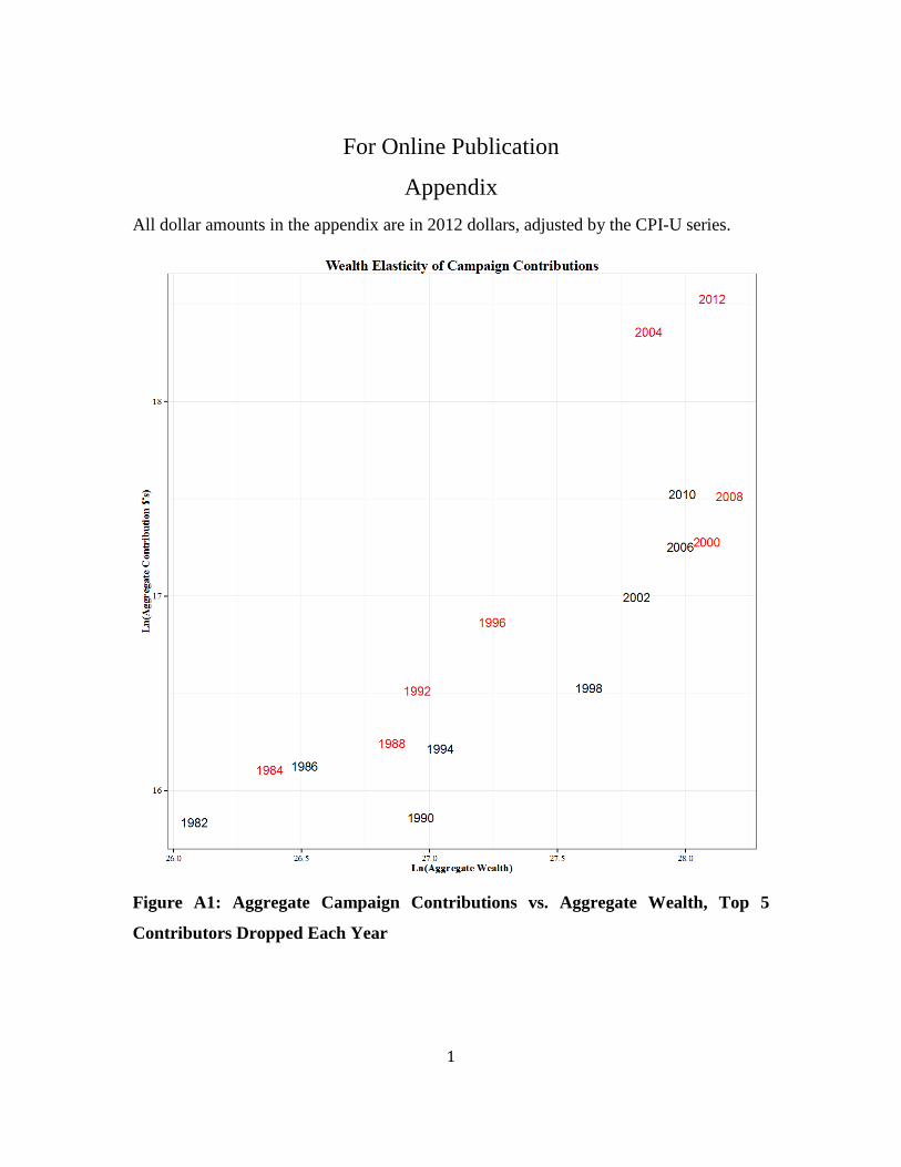
recent presidential years, 2004 and 2012. To check that the figure was not distorted by a

few large contributions, we redid the figure with the five largest contributions trimmed

from each year. Results are similar. (See the online Appendix.) The strong relationship

in figure 8 might reflect changes in the composition of the 400. In 2012, only exactly

half, 200, of the 400 members ten years earlier, in 2002, were still members. Naturally,

this group was relatively super wealthy since great wealth makes it less likely that one

will get bumped off the list by a new fortune. The 200 had 68% of the total wealth of the

400 in 2002. Nonetheless, their share had declined to 64% in 2012, implying that the

arrivals were relatively wealthier than the departures.

This observation suggests that wealth alone does not drive contribution and

that individual fixed effects, perhaps ideological in nature, may be important. Still, the

Forbes 400 clearly accounts for a growing share of contributions, nearing 5.0 percent in

2012 up from just 0.4 percent three decades earlier.

III. Data

We collected data on wealth and political contributions of all 1,510 individuals who

have appeared on the Forbes 400 annual list of the richest Americans from 1982 to 2013.

Our data is represented as an unbalanced panel of individuals across election cycles. Our

2 Estimates of net worth for Eychaner and Perry are provided by The Center for Public Integrity. See http://www.publicintegrity.org/2012/04/26/8754/meet-super-donor-all-stars.

7

dependent variable is contributions by individuals, aggregated over the two-year election

cycles.

Political Contributions

We include federal election contributions to candidates, party committees, and to

527s and super PACs. We do not include undisclosed contributions to 501c(3)s made

possible by Citizens United. Before 2013-14, these were relatively small. In addition,

small, unreported contributions, typically below $200 to an organization or candidate in

an election cycle have not been included. For more details, see Bonica, Rosenthal, and

Rothman (2014). The original data was drawn from the FEC and IRS web sites. The data

is maintained in the DIME database at Stanford. (data.stanford.edu/dime). The panel

dataset includes contributions for 400 members for all years from 1983-84 through 2011-

12 where the individual had reached voting age (18) and was not deceased.

Wealth

Our principal independent variable is wealth. We typically cannot measure wealth

for years in which the individual does not appear in the 400 list. For some years, Forbes

also lists the wealth of “drop offs”, those individuals who were in the list the preceding

year but whose wealth no longer suffices to put them in the 400. We use this information

where available. Otherwise, we adapt our methods to recognize that we have an upper

bound (subject to Forbes’s measurement error) on the wealth of the individual. That is,

we measure individual contributions for all years where the individual is alive and 21 and

older but, for individuals whose wealth is unmeasured by Forbes, we “know” only that

the individual’s wealth is below the minimum needed to be on the list. For individuals on

the list in both years of an election cycle, we measure their wealth as the average of their

wealth over the two years. For individuals on the list in only one year, we measure their

wealth as the average of their reported wealth in that year and the minimum threshold for

inclusion on the list in the other year. We exclude the 1981-1982 and 2013-2014 election

cycles from the regression analyses as we observed wealth in only one of the two-years

8

when we constructed our panel.3

Our results are robust to running the analysis with only

the observations where the individual belonged in both years of the cycle.

Record Linkage

Linking contribution records to 400 members is complicated by variations in

name and address. (To start, Forbes introduces variation in name across years.) We used

a combination of automated and directed matching to create our dataset, which contains

169,798 contribution records to federal elections made between 1983 and 2012. It

remains possible that the data contains errors. The entire dataset will be posted on a web

site. Corrections are welcome.

Covariates

We have information on the gender, age, and geographic location of residence of

the individual and rough measures of the source of wealth (finance, technology, oil, etc.).

We do not use that information in this study, but remove the effects of such variables

other through fixed effects. We do use age in cross-sectional estimates.

The Forbes 400: Potential Selection Effects

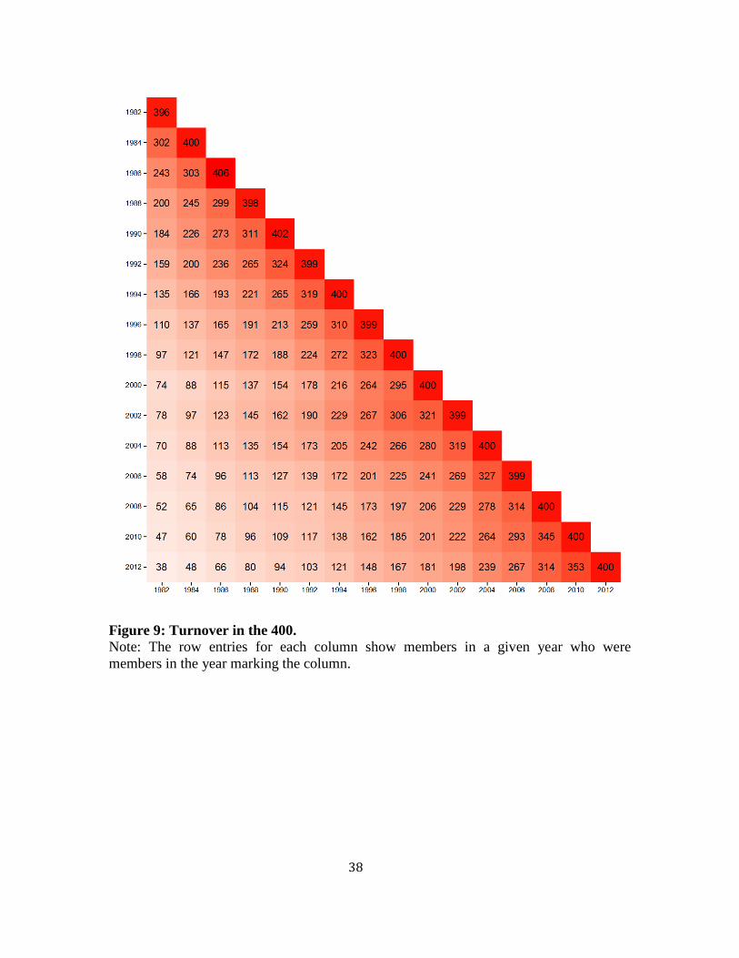
Membership in the Forbes 400 evolves extremely rapidly. Figure 9 cross-tabulates

membership by year. Only 38 members of the 1982 list also appear in 2012. Death is a

much less important part of the story than is entrepreneurial mobility. In an average year

in our panel, 6.9 individuals exited the list due to death, accounting for 14 percent of total

turnover. Death does generate dynastic turnover as, for example, when Sam Walton is

succeeded by his children. Longer dynasties, such as Du Ponts, Rockefellers, Fords, and

Marses, appear, but relatively young new entrepreneurial blood (Bill Gates, Mark

Zuckerberg, Michael Bloomberg, George Soros, Larry Ellison) is constantly entering.

Winners, like John Paulson, stick, and losers, like Raj Rajurtanam exit. As such, the

wealth of the 400 increases by selection.

3 We did use aggregate wealth for 2014 of the 400 in constructing figures 3, 4, and 5.

9

To see if the aggregate wealth elasticity represents more than selection, we

investigate individual wealth elasticity as well. We study if new blood is more politically

engaged by comparing average values of individual fixed effects across years.4

Heterogeneity of Contributions

There is considerable heterogeneity in contribution within the 400. In 2012, the

two largest donors both in the 400 and overall were Sheldon and Miriam Adelson, who

gave $56.8 million and $46.6 million, respectively. The Adelsons’ money may not have

been well spent, since most of it went to the presidential nomination bid of Newt

Gingrich. (We treat households like the Adelsons as a single household identified by the

main source of wealth. In this case, we treat Sheldon Adelson as contributing $103.4

million.) But, as said previously, only 39 other members gave over $1 million.

IV. Wealth Elasticity Results for the Forbes 400

We need to deal not only with strong variation in contributions across individuals

who do contribute but also with the variation in participation shown in Figure 2. To deal

with non-participation, our basic regression specification is tobit, as used by Gordon,

Hafer, and Landa (2007). The tobit is standard practice in studies of charitable giving, of

which campaign contributions can be thought of as a special case (Joulfaian 2000,

Wooldridge 2002, 518-19). We report the marginal effects of log wealth on the expected

value of log contributions evaluated at the mean value for explanatory variables. These

are in the row labeled “𝑑𝐸[𝑌]/𝑑x “ in the tables. Given that censoring is not severe, the

marginal effects are similar to the raw coefficients. Only 22 percent of observations in

our sample are left-censored compared to 65 percent for the sample used by Gordon,

Hafer, and Landa (2007). Heterogeneity of contributions is captured by individual fixed

effects.

Our first set of results pertains to an unbalanced panel of members of the 400

during their period of membership. We thus exclude, for the moment, contribution data

4 We do not include age in our panel analysis because age is highly collinear with the intertemporal pattern of both cycle fixed effects and individual fixed effects.

10

for individuals when they are non-members. We also, to estimate fixed effects, include

only individuals who have been members for at least two election cycles.

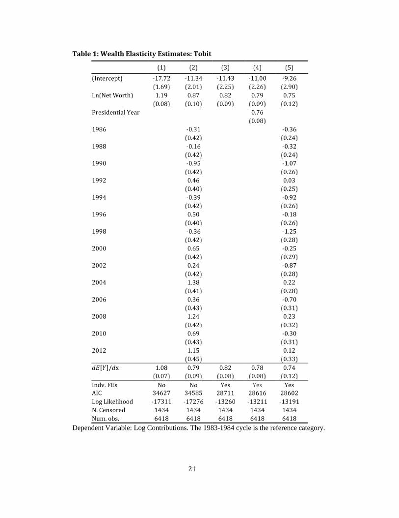
Our basic results appear in Table 1. The first model, with no fixed effects,

suggests that campaign contributions are a superior good since both the tobit coefficient

on wealth and the marginal effect are (slightly) greater than 1.0. Superiority goes away

with fixed effects. Models 2, 3, and 4, which alternate cycle and individual fixed effects

and presidential year dummy have elasticity estimates that are 0.87 or lower. The

estimated marginal effects all have z-statistics, with respect to 1.0, that are greater than 2.

If we replace cycle fixed effects with a presidential year dummy, we get the expected

result that more is given in presidential cycles. The elasticity drops to 0.74 with both

individual and cycle fixed effects. Still, the estimates in the range [0.74, 1.08] shown in

the table, given measurement error in wealth, are impressive and likely to be enough,

given the high rate of growth of wealth in the 400, to propel the 400 to a greater share of

total campaign giving.

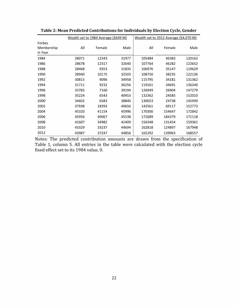
The increase in contributions by the 400 also reflects increasing fixed effects.

More precisely, a substantial portion of the increase in contributions by the 400 is a result

of current members, ceteris paribus, contributing more than members in earlier years.

This is shown by predicted contribution amounts displayed in Table 2. These are drawn

from the full specification, column 5 of Table 1. The Ns for the average in each cycle are

given in the diagonal elements of figure 9. They are either 400 or extremely close to it.

The first set of predicted values are calculated by setting each member’s wealth to the

average net worth of the 400 in 1984 ($649 M). For the second set of predicted values,

wealth is set to the average net worth of the 400 in 2012 ($4,070 M). Both sets of

predictions are calculated with election cycle fixed effects set to its 1984 value.

Individual fixed effects have clearly increased over the 30 years of our panel and have

done so within each gender. Comparing the first and last rows in column 1 suggests that

average contribution amounts would have increased from $28,071 in 1984 to $43,987 in

2012 due to turnover in membership alone. This compares to a predicted increase from

$28,071 to $105,484 assuming the average net worth of 1984 400 members had risen to

11

the 2012 level. A striking observation is that the predicted contribution amounts for

women are less than those for men in every cycle except 2006.5

Robustness

We next report on three robustness checks. The first includes the wealth of

individuals dropped off the 400. The second limits the time period. The third checks for

panel bias by using only individuals on the 400 for five or more election cycles.

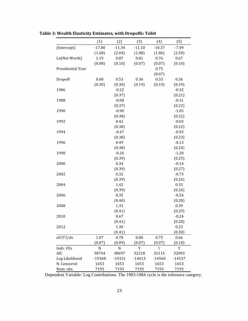
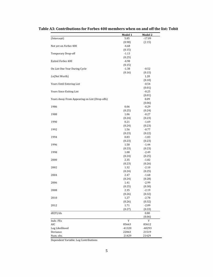
In recent years, Forbes has been reporting estimates of wealth of individuals who

dropped off the list in a given year. Including these estimates generates another 800

observations. The estimates reported in Table 3 show little change. A dummy for Drop-

off is positive but insignificant. We conducted further analysis with proxies for wealth

when wealth was not observed but the individual was over 21 years of age. Our basic

results hold in these specifications. Contributions are systematically lower when an

individual is not on the list. The decline is less when an individual leaves the list but

rejoins it later than when an individual permanently exits the list. Full details are in the

online Appendix.

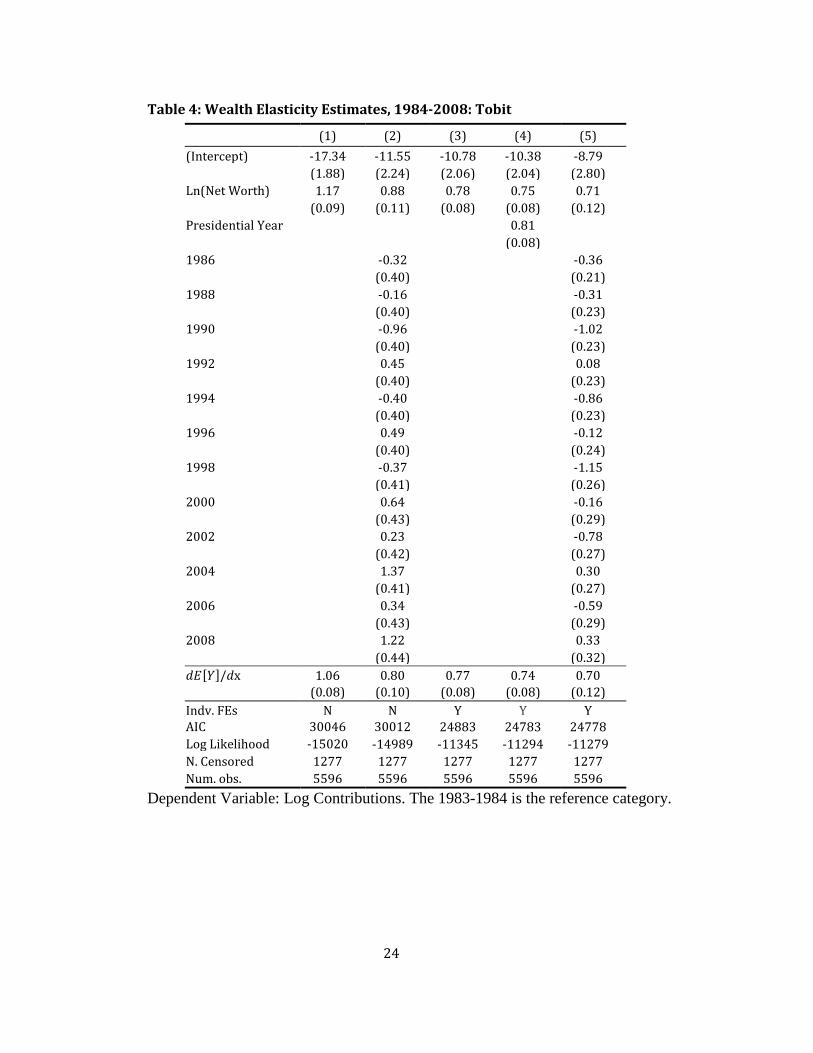
Because campaign finance may have been changed by the Citizens United

decision in 2010, we also report results restricted to the 1983-84 through 2007-08 cycle.

Again, results are robust, although the elasticity drops slightly with individual and cycle

fixed effects included, as shown in Table 4.

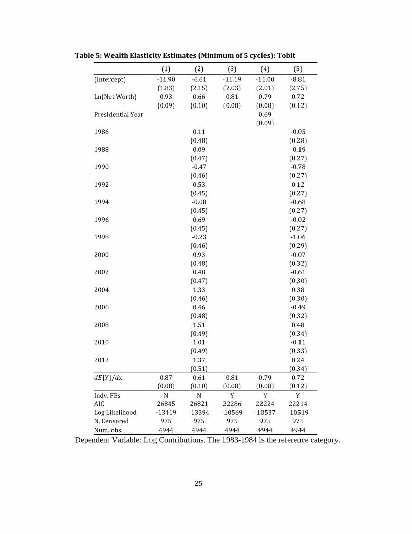
Our final robustness check limits the analysis to those on the 400 for five or more

cycles (generally 10 years) as against Table 1, where the sample includes those present in

two or more cycles. Again the results, shown in Table 5, are robust.

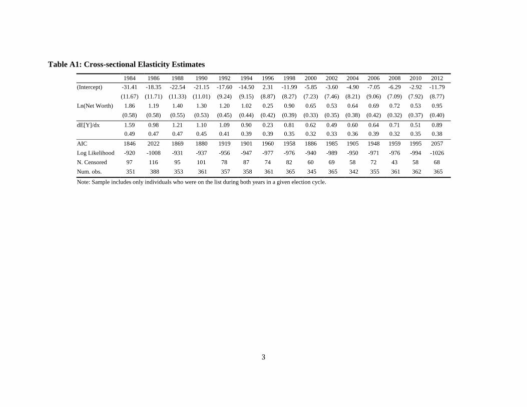
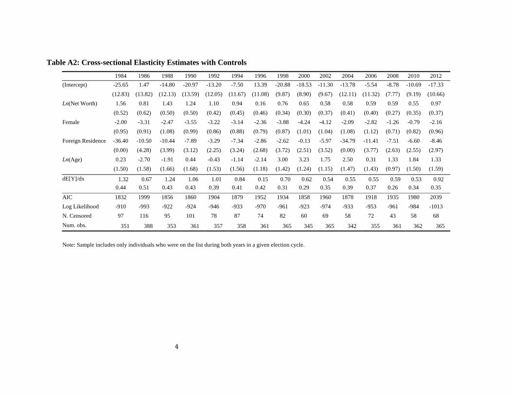
We include cross-sectional results by election cycle in the online appendix. We

estimate the cross-sectional regressions first without and then with controls for

individual-level characteristics including age, residence outside the United States, and

gender, which were subsumed by the fixed-effects in the panel regression. The cross-

5 The sudden increase in average contributions for women starting in 2004 is explained by entry onto the list by Marion Sandler, Linda Pritzker and Penny Pritzker. Were we to exclude these three observations from the calculations in column 2, the averages for women would have been much lower at $17,769 in 2004 and $19,719 in 2006.

12

sectional results are largely consistent with the panel estimates. The estimates for wealth

elasticity range from a maximum of 1.60 in 1984 to a minimum of 0.46 in 1996. In none

of the cross-sectional regressions do we reject the null that wealth elasticity is equal to

one. When individual-level controls are included, we find the coefficients for female and

residing outside of the United States are both consistently associated with reduced

contributions. We previously noted that the percentage of females in the 400 has

declined. Much female wealth may come from inheritance. Heirs may have less political

interest than entrepreneurs. Separating heirs from entrepreneurs, however, may be tricky.

The Koch brothers are heirs that grew their business. The estimated effects for age are not

consistent across elections cycles.

V. Wealth Elasticity Results from Census Tracts

The results above represent estimates of elasticity at the very extreme of the wealth

distribution. This leaves open the possibility that the estimates might differ when looking

at the overall distribution. Analogously, luxury yachts may look like a normal good when

looking only at the 400 but appear as a luxury good in looking at the entire wealth

distribution.

While we are unaware of any other comparable data sources with individual-level

data on wealth and campaign contributions, the American Community Survey (ACS)

provides estimates of household income and housing property values aggregated by

census tract. The total value of owner occupied housing provides an indirect measure of

wealth. We additionally estimate income elasticity using ACS estimates of per-capita

income by census tract. The dependent variable is log total contributions dollars

aggregated by census tract. In order to calculate the values, we overlay geo-coordinates

provided in the DIME data onto census tract shape files. To remain consistent with the 5-

year American Community Survey data which were collected between 2008 and 2012,

we include all federal contributions made during the three election cycles of 2008, 2010,

and 2012.

One limitation of this approach is the $200 disclosure threshold for federal

contributions. While this is unlikely to pose an issue for the 400, it will censor

contributions from the less well off. This could bias the contribution totals in lower and

middle-class neighborhoods downwards. Small donors, defined as those making “small

13

gifts” in amounts below the $200 minimum threshold for inclusion in itemized reports,

accounted for about 10-15 percent of total contributions in recent elections.

A similar but opposite limitation is in the wealth data. Housing wealth, while a large

fraction of the wealth of the 99%, is a small fraction of the wealth of the 400. The ratio of

housing values to wealth is likely to be lower in very affluent census tracts than in poorer

ones. Furthermore, housing values imperfectly measure housing wealth since the values

do not measure housing equity.

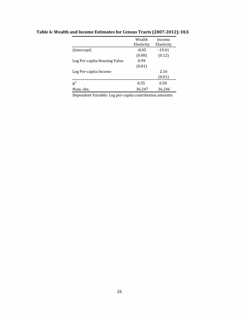
Table 6 reports the estimated elasticity with respect to (housing value) wealth and

income. The wealth elasticity estimate is very close to 1.00 and is consistent with the

Forbes estimates when controlling for cycle fixed-effects. This increases our confidence

of the validity of the Forbes estimation. It also provides added confidence in the finding

that contributions are in fact normal with respect to wealth and are not simply an artifact

of the sample. At the same time, the estimated income elasticity of 2.16 does indicate

campaign contributions are a superior good with respect to income. However, both

estimates may be slightly inflated due to the censoring problem discuss above.

We draw on contribution records from state elections in Ohio and Florida, which

do not have a minimum reporting thresholds and instead require that all contributions be

itemized, to assess sensitivity to the $200 threshold. We do so by estimating the wealth

and income elasticity first based on total amounts contributed to state elections by census

tract and then again based on total amounts from contributions of $200 or more. We

estimate the models separately for each state. The coefficient estimates do not appear to

be very sensitive to the reporting thresholds. The estimated coefficient on wealth

elasticity fell very slightly from 0.84 to 0.82 for Florida and from 0.85 to 0.82 in Ohio

after censoring contributions below $200. The corresponding estimates for income

elasticity before and censoring at $200 were 1.67 and 1.65 for Florida and 1.88 and 1.86

for Ohio.

VI. Wealth Effects for Republicans and Democrats

If increases in individual wealth lead to substantial increases in individual giving, the

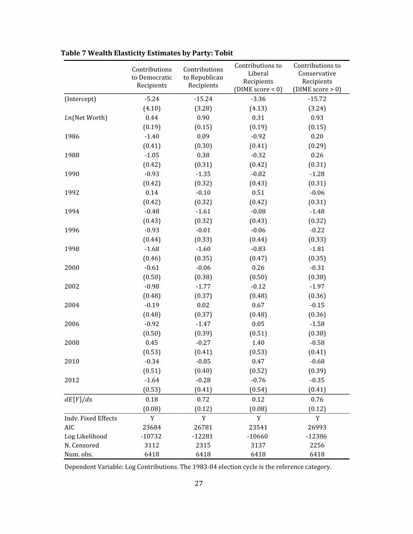
increases appear mainly to the benefit of Republicans. In Table 7, we report separate

estimates for Democratic and Republican contributions. So if an individual gave only to

14

Democrats, the individual would be recorded as a zero contributor to Republicans. Note

that the number of observations is identical to that in Table 1. The results show that the

elasticity is much higher for Republican donations than for those to Democrats. In fact,

the Democrat coefficient is quite close to zero.

An even sharper (if not statistically significantly so) difference occurs if we analyze

contributions in terms of a continuous measure of ideology. This measure, developed

from contribution data, is the common-space DIME score of Bonica (2014). The measure

corresponds well with the common notion of liberal and conservative and correlates

highly, for elected members of Congress, with the widely used DW-NOMINATE scores

of Poole and Rosenthal (2007). Illustrative scores for 400 members are David Koch, 0.88;

Sheldon Adelson, 0.76; Bill Gates, -.043; Warren Buffet, -0.78; George Soros, -1.08. We

separate liberal and conservative candidates on the basis of their DIME score, with a

score of 0 being the separating value. Even with fixed effects, contributions to

conservatives have an elasticity of nearly 1.0. The results are robust to restricting the

sample to those in the 400 for five or more cycles.

We explore the partisan differences further by running separate regressions for

individuals grouped into ideological camps. Individuals with strong partisan leanings,

defined as those who have given more than 90 percent of their contribution dollars to a

single party during the period of our panel (including years they were not 400 members),

are placed in the liberal and conservative groups. The dependent variable for each group

is log contributions to their respective parties. Non-donors and donors who have never

given to a candidate or committee affiliated with a major party are excluded from the

analysis. Breaking out donors by partisan leanings allows us to rule out concerns that the

lower estimated elasticity for giving to Democrats might be dragged down by zeroes

generated by conservatives who rarely support Democrats. The results, shown in Table 8,

are similar to those reported in Table 7.

We observe, to summarize this section, that were the composition of the 400 to

remain unchanged but the members’ wealth uniformly shifted upward, the Republicans

would be the beneficiaries of the shift in wealth. That is, supposing a one-percent across

the board increase in the net worth of the 400, the corresponding increase in contributions

going to Republicans would be 0.72 percent versus just 0.18 percent for Democrats.

15

VII. Partisan Preferences Are Insensitive to Changes in Wealth

Canonical models of redistribution offer some possible insights as to why wealth

effects differ by party. These models predict that preferences over redistribution are a

function of an individual’s income and the aggregate income of society (e.g. Meltzer and

Richard 1981, Bolton and Roland 1999). As an individual’s income increases relative to

society, her preferred level of redistribution will decrease. In a polarized two-party

system where the parties differ on their proposed levels of redistribution, support for the

anti-redistributive party is predicted to be increasing in relative income. A direct

implication is that demand for Republican and Democratic policies will behave as

superior and inferior substitute goods. If Individuals do in fact move to the right as wealth

increases, it could explain why the wealth elasticity is lower for Democrats.

There is strong empirical evidence of a relationship between income and

partisanship (e.g. McCarty, Poole, and Rosenthal 2006, Bonica, Rosenthal, and Rothman,

2014, 2015). However, the trend towards Democrats shown in Figure 6 suggests these

findings might not hold for the 400. Our data allow us to directly test this by examining

the preference dynamics of the Forbes 400 as revealed by their contribution patterns. We

construct two time-varying measures of political preferences. The first are period-specific

DIME scores. The dynamic ideal points are recovered by applying the one-period-at-a-

time estimation procedure developed by Nokken and Poole (2004) to the DIME scores

(See Bonica 2014 for details.) The technique estimates independent period-specific ideal

points for contributors made in each period, with the candidate ideal points held static.

This allows contributor ideal points to change freely from one cycle to the next. The

second measure is the percentage of contribution dollars made to Republican recipients

grouped by election cycle. We regress these preference measures on log wealth first

specified with a simple bivariate regression and then including fixed effects and

controlling for age.

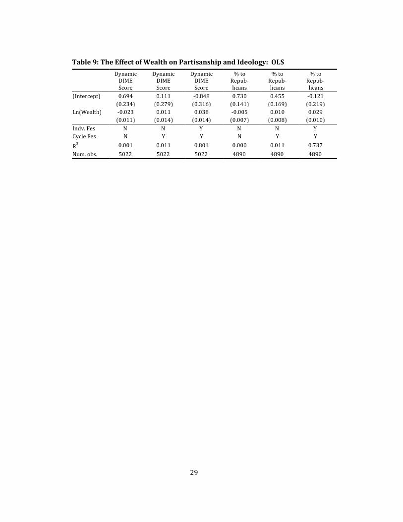
The results reported in Table 9 offer little evidence of a wealth effect on ideology.

Wealth alone fails to explain any of the variance in giving patterns. Only in the two-way

fixed effects model is the coefficient for wealth statistically significant. Even then, the

effect sizes are extremely small. To place the effect size in context, moving from the

16

average 400 net worth of $4 billion in 2012 to the top value of $63.4 billion would

correspond to a shift of just 0.12 of a standard deviation in overall DIME scores, or about

a third of the difference between Hillary and Bill Clinton. We further consider whether

contributors change before and after making it onto the list. We estimate separate DIME

scores for each individual based on contributions made before and after appearing on the

Forbes 400. A t-test of before and after estimates is not significant (t = 0.47).

Taken in context, the results suggest that if the first billion did not induce a

preference for Republican policies, it is unlikely the next ten billion will either. Insofar

as individual preferences respond to increases in wealth, the transition must typically

occur at a much earlier point in the wealth distribution. The evidence here is consistent

with the partisan stability of contributions by medical doctors (Bonica, Rothman, and

Rosenthal, 2014, 2015). It is also consistent with a long-standing view in political science

that partisan identification is fixed early in adult life and remains stable (Green, Shickler,

and Palmquist 2004).

VIII. Discussion

The increasing share of total contributions made by the Forbes 400 appears to reflect

two factors. First, entrants to the list are likely to be heavier contributors than those who

exit. Second, even though the elasticity of contribution with individual and cycle fixed

effects is less than 1.0, the elasticity appears large enough for continuing members to be

increasing their contributions at a higher rate than the growth of contributions in the

general population.

Does the Deregulation of Political Finance Account for Increased Inequality?

A robust regulatory framework governs the market for political contributions. It has

been widely speculated that the recent wave of successful legal challenges brought

against the Federal Election Commission—notably the rulings in Supreme Court rulings

in Citizens United vs. FEC and McCutcheon vs. FEC—are primarily responsible for the

increased concentration of campaign contributions. It stands to reason that contribution

limits that cap direct donations to candidates during an election cycle at a few thousand

dollars, while intended to keep most legislative services and favors priced out of the

market, also artificially constrains spending on politics well below what demand would

dictate in an unregulated market (McCarty and Rothenberg 1997; Ansolabehere et. al

17

2003). While changes to the regulatory environment have likely contributed to the trend,

our results suggest they provide at best a partial explanation. There are no big jumps in

our data that correspond to changes in campaign finance law.

It is possible that accounts focusing on changes to campaign finance laws have

overestimated their practical importance. Granted, supposing the enactment of a legal

environment where hard-money limits were strictly binding and soft-money and

independent expenditure loopholes were closed, sustaining the current levels of

inequality in campaign contributions would be infeasible. However, the legal framework

for individuals to donate unlimited amounts was set in place decades earlier by Buckley v.

Valeo (424 US 1 [1976]).

Partisan Trends in Giving by the Forbes 400

The shifting partisan leanings of the nation’s wealthiest individuals have

implications for understanding recent trends in political fundraising. The historic rise in

inequality in recent decades has not ushered in an era of Republican fundraising

dominance. On the contrary, we have seen the exact opposite. Democrats have made

substantial gains against Republicans in recent decades while inequality was on the rise.

In the 1980s, Democrats faced a sizable fundraising deficit, often being outraised in

Congressional races by a 2:1 margin. By 2004, Democrats had closed the gap and have

since managed to outraise Republicans in two of the past six election cycles. These trends

are partly attributable to strong support for Democrats among high earning professionals.

Our results show that these patterns extend to the wealthiest members of society, owing

in part to the growth of technology sector. The relative political benefits to parties will

nonetheless depend heavily on the partisan leanings of entrants to the Forbes 400, which

are in turn related to sources of wealth.

Contributions depend heavily on partisan efforts at fund-raising. But donors also

structure the process as noted by the activity of the Koch brothers and the Adelsons on

the Republican side and by the engagement with and disengagement from Barack Obama

by George Soros. Whether the impetus is from politicians or contributors or self-spenders

such as Ross Perot and Donald Trump, much of the money may not find its way to

supporting the candidates of the two major parties but is dissipated in primaries or third

party runs. Competitive spending in the out party, as with the Republicans for 2016 and

18

the Democrats for 2004, may be important to short-term variations in how the wealthy

support the two major parties. Our results show, however, a definite long-term trend to

the Democrats.

VIII. Conclusion

We have shown the campaign contributions by members of the 400 are sensitive to

changes in the wealth of the individuals. One might be concerned about the endogeneity

of wealth with respect to contributions. This is only a partial concern. Entrepreneurs such

as Bill Gates, Sergey Brin, Larry Page, George Soros, and Mark Zuckerberg got wealthy

before they became contributors. Gates, Brin, Page, and Zuckerberg made no

contributions in election cycles prior to joining the 400. Those of Soros were well under

$10,000 per cycle. On the other hand, established wealth may contribute to preserve or

increase wealth by items like the carried interest deduction, the diminished estate tax, and

special treatment for the fossil fuels sector. The question must be left to future research.

The increasing concentration of campaign contributions is likely to be responsive

to the increase in economic inequality. On the other hand, the wealth elasticity is largely

a matter that affects Republican or conservative contributors.

19

References

Ansolabehere, Stephen, John M. de Figueredo, and James Snyder. 2003. “Why is There

So Little Money in Politics?” Journal of Economic Perspectives, 17(1):105-130.

Bonica, Adam. 2014. “Mapping the Ideological Marketplace”. American Journal of

Political Science, 58 (2): 367- 387.

Bonica, Adam, Nolan McCarty, Keith T. Poole, and Howard Rosenthal, 2013. “Why

Hasn’t Democracy Slowed Rising Inequality?” Journal of Economic Perspectives

27(3): 103-24.

Bonica, Adam, Howard Rosenthal, and David Rothman. 2014. “The Political Polarization

of Physicians in the United States: An Analysis of Campaign Contributions to

Federal Elections, 1991-2012” JAMA Internal Medicine. 174 (8): 1308-1317.

Bonica, Adam, Howard Rosenthal, and David Rothman. 2015. “The Political Alignment

of US Physicians: An Update Including Campaign Contributions to the

Congressional Midterm Elections in 2014” JAMA Internal Medicine. 175(7):1236-

1237.

Bolton, Patrick and Gerard Roland. 1999. “The Break-up of Nations.” Quarterly Journal

of Economics 112(4):1057-1090.

Edlund, Lena and Wojciech Kopczuk, 2009. "Women, Wealth, and Mobility”, American

Economic Review, 99 (1): 146-178.

Green, Donald P., Bradley Palmquist, and Eric Schickler. Partisan Hearts and Minds:

Political Parties and The Social Identities of Voters. Yale University Press, 2004.

Gordon, Sanford, Catherine Hafer, and Dmitri Landa. 2007. “Consumption or

Investment? On Motivations for Political Giving.” Journal of Politics, 69:1057-72

Joulfaian, David. 2000. "Estate Taxes and Charitable Bequests by the Wealthy” National

Tax Journal National Tax Association, 53(n3): 743-64, September.

Kopczuk, Wojciech and Emmanuel Saez 2004. "Top Wealth Shares in the United States,

1916-2000: Evidence from Estate Tax Returns", short version National Tax Journal,

57(2), Part 2, June, 445-487 (long NBER Working Paper No. 10399, March)

Malkiel, Burton, 2015, A Random Walk Down Wall Street: The Time-Tested Strategy for

Successful Investing (Eleventh Edition), New York, W. W. Norton.

20

McCarty, Nolan, Keith T. Poole, and Howard Rosenthal. Polarized America: The Dance

of Ideology and Unequal Riches. Cambridge, MA. MIT Press, 2006.

McCarty, Nolan, and Lawrence S. Rothenberg. 1996. "Commitment and the Campaign

Contribution Contract." American Journal of Political Science no. 40 (3):872-904.

Piketty, Thomas and Emmanuel Saez, 2003. "Income Inequality in the United States,

1913-1998” Quarterly Journal of Economics, 118(1), 1-39

Saez, Emmanuel and Gabriel Zucman, 2014. “Wealth Inequality in the United States

since 1913: Evidence from Capitalized Income Tax Data” NBER Working Paper

20625

Wooldridge, Jeffrey. 2002. Econometric Analysis of Cross Section and Panel Data.

Cambridge, MA: MIT Press

http://eml.berkeley.edu/~saez/pikettyqje.pdf�

http://eml.berkeley.edu/~saez/pikettyqje.pdf�

21

Table 1: Wealth Elasticity Estimates: Tobit

(1) (2) (3) (4) (5) (Intercept) -17.72 -11.34 -11.43 -11.00 -9.26

(1.69) (2.01) (2.25) (2.26) (2.90) Ln(Net Worth) 1.19 0.87 0.82 0.79 0.75

(0.08) (0.10) (0.09) (0.09) (0.12) Presidential Year 0.76 (0.08) 1986 -0.31 -0.36 (0.42) (0.24) 1988 -0.16 -0.32 (0.42) (0.24) 1990 -0.95 -1.07 (0.42) (0.26) 1992 0.46 0.03 (0.40) (0.25) 1994 -0.39 -0.92 (0.42) (0.26) 1996 0.50 -0.18 (0.40) (0.26) 1998 -0.36 -1.25 (0.42) (0.28) 2000 0.65 -0.25 (0.42) (0.29) 2002 0.24 -0.87 (0.42) (0.28) 2004 1.38 0.22 (0.41) (0.28) 2006 0.36 -0.70 (0.43) (0.31) 2008 1.24 0.23 (0.42) (0.32) 2010 0.69 -0.30 (0.43) (0.31) 2012 1.15 0.12 (0.45) (0.33) 𝑑𝐸[𝑌]/𝑑x 1.08 0.79 0.82 0.78 0.74

(0.07) (0.09) (0.08) (0.08) (0.12) Indv. FEs No No Yes Yes Yes AIC 34627 34585 28711 28616 28602 Log Likelihood -17311 -17276 -13260 -13211 -13191 N. Censored 1434 1434 1434 1434 1434 Num. obs. 6418 6418 6418 6418 6418

Dependent Variable: Log Contributions. The 1983-1984 cycle is the reference category.

22

Table 2: Mean Predicted Contributions for Individuals by Election Cycle, Gender Wealth set to 1984 Average ($649 M) Forbes Membership

Wealth set to 2012 Average ($4,070 M)

in Year All Female Male All Female Male

1984 28071 12343 31977 105484 46383 120162 1986 28678 12317 32640 107764 46282 122652 1988 28468 9353 31835 106976 35147 119629 1990 28940 10175 32503 108750 38235 122136 1992 30815 9096 34958 115795 34181 131362 1994 31711 9232 36256 119161 34691 136240 1996 33783 7160 39194 126949 26904 147279 1998 35224 6543 40453 132362 24585 152010 2000 34602 6583 38840 130023 24738 145949 2002 37938 18393 40656 142561 69117 152773 2004 45320 41154 45996 170300 154647 172842 2006 45956 49067 45538 172689 184379 171118 2008 41607 34982 42409 156348 131454 159361 2010 43329 33237 44694 162818 124897 167948 2012 43987 37247 44856 165292 139963 168557

Notes: The predicted contribution amounts are drawn from the specification of Table 1, column 5. All entries in the table were calculated with the election cycle fixed effect set to its 1984 value, 0.

23

Table 3: Wealth Elasticity Estimates, with Dropoffs: Tobit

(1) (2) (3) (4) (5) (Intercept) -17.80 -11.34 -11.10 -10.37 -7.49

(1.68) (2.04) (1.88) (1.86) (2.50) Ln(Net Worth) 1.19 0.87 0.81 0.76 0.67

(0.08) (0.10) (0.07) (0.07) (0.10) Presidential Year 0.75

(0.07) Dropoff 0.68 0.53 0.36 0.33 0.36 (0.30) (0.30) (0.19) (0.19) (0.19) 1986 -0.22 -0.32 (0.37) (0.21) 1988 -0.08 -0.31 (0.37) (0.22) 1990 -0.90 -1.05 (0.38) (0.22) 1992 0.42 -0.03 (0.38) (0.22) 1994 -0.47 -0.93 (0.38) (0.23) 1996 0.49 -0.13 (0.38) (0.24) 1998 -0.26 -1.20 (0.39) (0.25) 2000 0.34 -0.14 (0.39) (0.27) 2002 0.32 -0.73 (0.39) (0.26) 2004 1.42 0.33 (0.39) (0.26) 2006 0.35 -0.54 (0.40) (0.28) 2008 1.33 0.39 (0.41) (0.29) 2010 0.67 -0.24 (0.41) (0.28) 2012 1.30 0.23 (0.41) (0.30) 𝑑𝐸[𝑌]/𝑑x 1.07 0.78 0.80 0.75 0.66

(0.07) (0.09) (0.07) (0.07) (0.10) Indv. FEs N N Y Y Y AIC 38744 38697 32218 32115 32093 Log Likelihood -19368 -19331 -14613 -14560 -14537 N. Censored 1653 1653 1653 1653 1653 Num. obs. 7193 7193 7193 7193 7193

Dependent Variable: Log Contributions. The 1983-1984 cycle is the reference category.

24

Table 4: Wealth Elasticity Estimates, 1984-2008: Tobit

(1) (2) (3) (4) (5) (Intercept) -17.34 -11.55 -10.78 -10.38 -8.79

(1.88) (2.24) (2.06) (2.04) (2.80) Ln(Net Worth) 1.17 0.88 0.78 0.75 0.71


(0.08) 1986 -0.32 -0.36 (0.40) (0.21) 1988 -0.16 -0.31 (0.40) (0.23) 1990 -0.96 -1.02 (0.40) (0.23) 1992 0.45 0.08 (0.40) (0.23) 1994 -0.40 -0.86 (0.40) (0.23) 1996 0.49 -0.12 (0.40) (0.24) 1998 -0.37 -1.15 (0.41) (0.26) 2000 0.64 -0.16 (0.43) (0.29) 2002 0.23 -0.78 (0.42) (0.27) 2004 1.37 0.30 (0.41) (0.27) 2006 0.34 -0.59 (0.43) (0.29) 2008 1.22 0.33 (0.44) (0.32) 𝑑𝐸[𝑌]/𝑑x 1.06 0.80 0.77 0.74 0.70


Dependent Variable: Log Contributions. The 1983-1984 is the reference category.

25

Table 5: Wealth Elasticity Estimates (Minimum of 5 cycles): Tobit

(1) (2) (3) (4) (5) (Intercept) -11.90 -6.61 -11.19 -11.00 -8.81

(1.83) (2.15) (2.03) (2.01) (2.75) Ln(Net Worth) 0.93 0.66 0.81 0.79 0.72


(0.09) 1986 0.11 -0.05 (0.48) (0.28) 1988 0.09 -0.19 (0.47) (0.27) 1990 -0.47 -0.78 (0.46) (0.27) 1992 0.53 0.12 (0.45) (0.27) 1994 -0.08 -0.68 (0.45) (0.27) 1996 0.69 -0.02 (0.45) (0.27) 1998 -0.23 -1.06 (0.46) (0.29) 2000 0.93 -0.07 (0.48) (0.32) 2002 0.48 -0.61 (0.47) (0.30) 2004 1.33 0.38 (0.46) (0.30) 2006 0.46 -0.49 (0.48) (0.32) 2008 1.51 0.48 (0.49) (0.34) 2010 1.01 -0.11 (0.49) (0.33) 2012 1.37 0.24 (0.51) (0.34) 𝑑𝐸[𝑌]/𝑑x 0.87 0.61 0.81 0.79 0.72


Dependent Variable: Log Contributions. The 1983-1984 is the reference category.

26

Table 6: Wealth and Income Estimates for Census Tracts (2007-2012): OLS

Wealth

Elasticity Income

Elasticity (Intercept) -8.05 -19.41

(0.08) (0.12) Log Per-capita Housing Value 0.99 (0.01) Log Per-capita Income 2.16

(0.01)

R2 0.35 0.50 Num. obs. 36,247 36,246 Dependent Variable: Log per-capita contribution amounts

27

Table 7 Wealth Elasticity Estimates by Party: Tobit

Contributions to Democratic

Recipients

Contributions to Republican

Recipients

Contributions to Liberal

Recipients (DIME score < 0)

Contributions to Conservative

Recipients (DIME score > 0)

(Intercept) -5.24 -15.24 -3.36 -15.72

(4.10) (3.28) (4.13) (3.24) 𝐿𝑛(Net Worth) 0.44 0.90 0.31 0.93

(0.19) (0.15) (0.19) (0.15) 1986 -1.40 0.09 -0.92 0.20 (0.41) (0.30) (0.41) (0.29) 1988 -1.05 0.38 -0.32 0.26 (0.42) (0.31) (0.42) (0.31) 1990 -0.93 -1.35 -0.82 -1.28 (0.42) (0.32) (0.43) (0.31) 1992 0.14 -0.10 0.51 -0.06 (0.42) (0.32) (0.42) (0.31) 1994 -0.48 -1.61 -0.08 -1.48 (0.43) (0.32) (0.43) (0.32) 1996 -0.93 -0.01 -0.06 -0.22 (0.44) (0.33) (0.44) (0.33) 1998 -1.68 -1.60 -0.83 -1.81 (0.46) (0.35) (0.47) (0.35) 2000 -0.61 -0.06 0.26 -0.31 (0.50) (0.38) (0.50) (0.38) 2002 -0.98 -1.77 -0.12 -1.97 (0.48) (0.37) (0.48) (0.36) 2004 -0.19 0.02 0.67 -0.15 (0.48) (0.37) (0.48) (0.36) 2006 -0.92 -1.47 0.05 -1.58 (0.50) (0.39) (0.51) (0.38) 2008 0.45 -0.27 1.40 -0.58 (0.53) (0.41) (0.53) (0.41) 2010 -0.34 -0.85 0.47 -0.68 (0.51) (0.40) (0.52) (0.39) 2012 -1.64 -0.28 -0.76 -0.35 (0.53) (0.41) (0.54) (0.41) 𝑑𝐸[𝑌]/𝑑x 0.18 0.72 0.12 0.76

(0.08) (0.12) (0.08) (0.12) Indv. Fixed Effects Y Y Y Y AIC 23684 26781 23541 26993 Log Likelihood -10732 -12281 -10660 -12386 N. Censored 3112 2315 3137 2256 Num. obs. 6418 6418 6418 6418

Dependent Variable: Log Contributions. The 1983-84 election cycle is the reference category.

28

Table 8. Wealth Elasticity Estimates for Donors Grouped By Partisan Leanings: Tobit

Democratic

Donors Democratic

Donors Democratic

Donors Republican

Donors Republican

Donors Republican

Donors (Intercept) -15.76 -0.26 8.06 -20.50 -13.85 -4.11

(6.36) (7.79) (8.99) (3.48) (4.32) (5.04) 𝐿𝑛(Net Worth) 1.05 0.27 0.25 1.32 1.00 0.82

(0.30) (0.39) (0.45) (0.17) (0.21) (0.23) 1986 -2.89 -2.37 0.04 -0.20 (1.50) (0.82) (0.74) (0.43) 1988 -0.79 -0.79 -0.20 -0.19 (1.47) (0.85) (0.77) (0.48) 1990 -2.17 -2.17 -1.31 -1.38 (1.45) (0.86) (0.77) (0.48) 1992 1.46 0.88 0.07 -0.37 (1.45) (0.85) (0.76) (0.47) 1994 0.24 -0.87 -0.95 -1.50 (1.43) (0.87) (0.77) (0.48) 1996 2.31 1.65 0.30 -0.65 (1.44) (0.91) (0.76) (0.49) 1998 0.29 -0.19 -0.83 -1.68 (1.47) (0.99) (0.78) (0.52) 2000 1.34 0.20 0.74 0.10 (1.48) (1.06) (0.81) (0.57) 2002 0.83 -0.73 -0.35 -0.94 (1.46) (1.04) (0.79) (0.55) 2004 2.19 0.55 1.76 0.83 (1.46) (1.04) (0.78) (0.55) 2006 0.95 -0.98 -0.08 -0.67 (1.52) (1.12) (0.81) (0.59) 2008 2.47 0.85 0.95 0.27 (1.50) (1.18) (0.84) (0.63) 2010 1.28 -0.57 0.52 -0.05 (1.50) (1.13) (0.83) (0.61) 2012 2.03 0.32 1.38 0.85 (1.52) (1.16) (0.86) (0.63) 𝑑𝐸[𝑌]/𝑑x 0.86 0.22 0.24 1.19 0.90 0.81

(0.25) (0.31) (0.42) (0.15) (0.19) (0.23) Indv. Fes N N Y N N Y AIC 4716 4700 3894 9554 9551 8196 Log-Lik -2355 -2333 -1767 -4774 -4759 -3780 N. Censored 265 272 265 405 405 405 Num. obs. 881 881 881 1764 1764 1764

Dependent Variable: Log Contributions. The 1983-84 election cycle is the reference category.

29

Table 9: The Effect of Wealth on Partisanship and Ideology: OLS

Dynamic DIME Score

Dynamic DIME Score

Dynamic DIME Score

% to Repub- licans

% to Repub- licans

% to Repub- licans

(Intercept) 0.694 0.111 -0.848 0.730 0.455 -0.121

(0.234) (0.279) (0.316) (0.141) (0.169) (0.219) Ln(Wealth) -0.023 0.011 0.038 -0.005 0.010 0.029

(0.011) (0.014) (0.014) (0.007) (0.008) (0.010) Indv. Fes N N Y N N Y Cycle Fes N Y Y N Y Y

R2 0.001 0.011 0.801 0.000 0.011 0.737 Num. obs. 5022 5022 5022 4890 4890 4890

30

Figure 1: Concentration of Wealth and Campaign Contributions in the Top 0.01 Percent of Households and Voting Age Population Note: The dark line tracks the share of campaign contributions in federal elections given by the top 0.01 percent of the voting age population. See Bonica et al. (2013) for details on how the trend was constructed. The shaded lines track the share of total private wealth owned by the top 0.01 percent of households as measured by Saez and Zucman (2014) by capitalizing income tax data (solid line) and by Kopczuk and Saez (2004) estimated from estate tax returns (dashed line). Both measures were obtained from http://eml.berkeley.edu/~saez/.

http://eml.berkeley.edu/~saez/�

31

Figure 1: Percentage of Forbes 400 Contributing to Federal Elections by Cycle. Figure 2: Percentage of Forbes 400 Contributing to Federal Elections by Cycle.

32

Figure 3: Growth of Forbes 400 Aggregate Wealth vs. S&P 500 Index (Nominal).

Note: The Forbes 400 starts in 1982. Figures that show only wealth could start in 1982.

Figures showing contributions start in 1984 because of our use of two-year election cycles.

The absence of Forbes data for 1981 resulted in our first election cycle being 1983-84.

33

Figure 4: Combined Wealth of the Forbes 400 Richest Americans (in 2014 Dollars).

Notes: Y-axis is log-scaled. The Forbes 400 starts in 1982. Figures that show only wealth could

start in 1982. Figures showing contributions start in 1984 because of our use of two-year election

cycles. The absence of Forbes data for 1981 resulted in our first election cycle being 1983-84.

34

Figure 5: Year-over-Year Increase in the Wealth Share of the Forbes 400.

35

Figure 6: Average Percentage Given to Republicans

36

Figure 7: Wealth and contribution shares of the Forbes 400 and the top 400 donors.

37

Figure 8: Wealth and Campaign Contributions. Note: Presidential years in red.

38

Figure 9: Turnover in the 400. Note: The row entries for each column show members in a given year who were members in the year marking the column.

1

For Online Publication

Appendix All dollar amounts in the appendix are in 2012 dollars, adjusted by the CPI-U series.

Figure A1: Aggregate Campaign Contributions vs. Aggregate Wealth, Top 5

Contributors Dropped Each Year

2

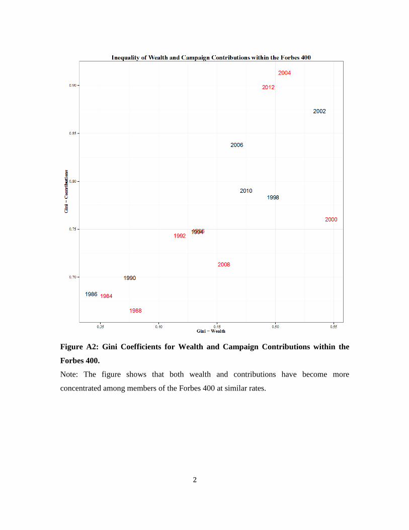
Figure A2: Gini Coefficients for Wealth and Campaign Contributions within the

Forbes 400.

Note: The figure shows that both wealth and contributions have become more

concentrated among members of the Forbes 400 at similar rates.

3

Table A1: Cross-sectional Elasticity Estimates

1984 1986 1988 1990 1992 1994 1996 1998 2000 2002 2004 2006 2008 2010 2012 (Intercept) -31.41 -18.35 -22.54 -21.15 -17.60 -14.50 2.31 -11.99 -5.85 -3.60 -4.90 -7.05 -6.29 -2.92 -11.79

(11.67) (11.71) (11.33) (11.01) (9.24) (9.15) (8.87) (8.27) (7.23) (7.46) (8.21) (9.06) (7.09) (7.92) (8.77)

Ln(Net Worth) 1.86 1.19 1.40 1.30 1.20 1.02 0.25 0.90 0.65 0.53 0.64 0.69 0.72 0.53 0.95

(0.58) (0.58) (0.55) (0.53) (0.45) (0.44) (0.42) (0.39) (0.33) (0.35) (0.38) (0.42) (0.32) (0.37) (0.40)

dE[Y]/dx 1.59 0.98 1.21 1.10 1.09 0.90 0.23 0.81 0.62 0.49 0.60 0.64 0.71 0.51 0.89

0.49 0.47 0.47 0.45 0.41 0.39 0.39 0.35 0.32 0.33 0.36 0.39 0.32 0.35 0.38

AIC 1846 2022 1869 1880 1919 1901 1960 1958 1886 1985 1905 1948 1959 1995 2057 Log Likelihood -920 -1008 -931 -937 -956 -947 -977 -976 -940 -989 -950 -971 -976 -994 -1026 N. Censored 97 116 95 101 78 87 74 82 60 69 58 72 43 58 68 Num. obs. 351 388 353 361 357 358 361 365 345 365 342 355 361 362 365

Note: Sample includes only individuals who were on the list during both years in a given election cycle.

4

Table A2: Cross-sectional Elasticity Estimates with Controls

1984 1986 1988 1990 1992 1994 1996 1998 2000 2002 2004 2006 2008 2010 2012

(Intercept) -25.65 1.47 -14.80 -20.97 -13.20 -7.50 13.39 -20.88 -18.53 -11.30 -13.78 -5.54 -8.78 -10.69 -17.33

(12.83) (13.82) (12.13) (13.59) (12.05) (11.67) (11.08) (9.87) (8.90) (9.67) (12.11) (11.32) (7.77) (9.19) (10.66)

Ln(Net Worth) 1.56 0.81 1.43 1.24 1.10 0.94 0.16 0.76 0.65 0.58 0.58 0.59 0.59 0.55 0.97

(0.52) (0.62) (0.50) (0.50) (0.42) (0.45) (0.46) (0.34) (0.30) (0.37) (0.41) (0.40) (0.27) (0.35) (0.37)

Female -2.00 -3.31 -2.47 -3.55 -3.22 -3.14 -2.36 -3.88 -4.24 -4.12 -2.09 -2.82 -1.26 -0.79 -2.16

(0.95) (0.91) (1.08) (0.99) (0.86) (0.88) (0.79) (0.87) (1.01) (1.04) (1.08) (1.12) (0.71) (0.82) (0.96)

Foreign Residence -36.40 -10.50 -10.44 -7.89 -3.29 -7.34 -2.86 -2.62 -0.13 -5.97 -34.79 -11.41 -7.51 -6.60 -8.46

(0.00) (4.28) (3.99) (3.12) (2.25) (3.24) (2.68) (3.72) (2.51) (3.52) (0.00) (3.77) (2.63) (2.55) (2.97)

Ln(Age) 0.23 -2.70 -1.91 0.44 -0.43 -1.14 -2.14 3.00 3.23 1.75 2.50 0.31 1.33 1.84 1.33

(1.50) (1.58) (1.66) (1.68) (1.53) (1.56) (1.18) (1.42) (1.24) (1.15) (1.47) (1.43) (0.97) (1.50) (1.59)

dE[Y]/dx 1.32 0.67 1.24 1.06 1.01 0.84 0.15 0.70 0.62 0.54 0.55 0.55 0.59 0.53 0.92

0.44 0.51 0.43 0.43 0.39 0.41 0.42 0.31 0.29 0.35 0.39 0.37 0.26 0.34 0.35

AIC 1832 1999 1856 1860 1904 1879 1952 1934 1858 1960 1878 1918 1935 1980 2039 Log Likelihood -910 -993 -922 -924 -946 -933 -970 -961 -923 -974 -933 -953 -961 -984 -1013 N. Censored 97 116 95 101 78 87 74 82 60 69 58 72 43 58 68 Num. obs. 351 388 353 361 357 358 361 365 345 365 342 355 361 362 365

Note: Sample includes only individuals who were on the list during both years in a given election cycle.

5

Table A3: Contributions for Forbes 400 members when on and off the list: Tobit

Model 1 Model 2 (Intercept) 5.85 -17.09

(0.98) (2.15) Not yet on Forbes 400 -4.68 (0.15) Temporary Drop-off -1.13 (0.25) Exited Forbes 400 -4.98 (0.15) On List One Year During Cycle -1.38 -0.52 (0.16) (0.15) 𝐿𝑛(Net Worth) 1.20 (0.10) Years Until Entering List -0.54 (0.01) Years Since Exiting List -0.25 (0.01) Years Away From Appearing on List (Drop-offs) 0.09 (0.06) 1986 0.06 -0.29

(0.25) (0.24) 1988 1.06 -0.27

(0.24) (0.23) 1990 0.21 -1.69

(0.24) (0.23) 1992 1.56 -0.77

(0.23) (0.22) 1994 0.83 -1.83

(0.23) (0.23) 1996 1.58 -1.44

(0.23) (0.23) 1998 1.08 -2.49

(0.24) (0.25) 2000 2.35 -1.82

(0.23) (0.26) 2002 1.32 -2.10

(0.24) (0.25) 2004 2.47 -1.68

(0.24) (0.28) 2006 1.41 -2.99

(0.25) (0.30) 2008 2.35 -2.19

(0.26) (0.32) 2010 1.27 -2.78

(0.26) (0.32) 2012 1.71 -2.09

(0.27) (0.33) dE[Y]/dx 0.80 (0.06) Indv. FEs Y Y AIC 85663 83612 Log Likelihood -41320 -40293 Deviance 22063 21519 Num. obs. 21429 21429 Dependent Variable: Log Contributions

6

We do not observe wealth estimates for most individuals during periods they were

not on the list. We collected data on dates of death.6

For individuals who are not currently on the list, we set their net worth to the

minimum threshold for inclusion on the list in a given year, which is same as the value of

the 400th ranked member. We then include controls for the number of years away from

the list an individual is relative to the closest year from when the individual is on the list.

This reflects that wealth should be closer to the minimum threshold for inclusion on the

list the closer an individual is to membership. Likewise, for years between appearing on

the list, we include a control for the duration in years from the last/next time an

individual will appear on the list. This is calculated as the absolute distance between the

current year and the most proximate year the individual appeared on the list. The

variables Years Until Entering List, Years Since Exiting List, and Years Away from

Appearing on List (Drop-offs) all take on values of zero for periods where an individual

appears on the list.

This makes it possible to determine

which past-members who have dropped off the list were alive after the last cycle where

they appeared on the list. We also observe when individuals on the list become of voting

age and can legally donate to campaigns.

Model 1 confirms that total giving is much greater when individuals are on the list

than either before entering or after exiting. The estimate for Temporary Drop-offs

indicates that individuals who temporally drop-off of the list but later rejoin it experience

a smaller decline in giving relative to either the run up to joining the list or following

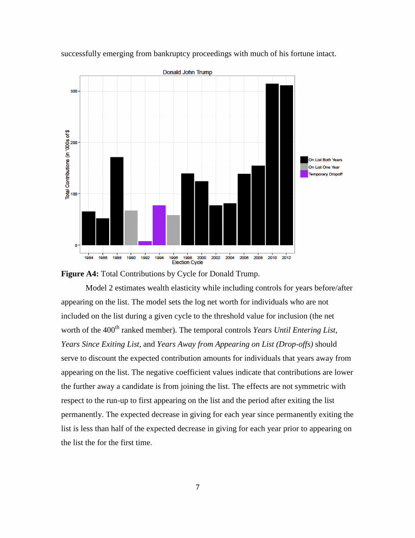
falling off the list permanently. Donald Trump offers an illustration of this dropoff effect.

Trump first appears on the list in 1982 and remains on it for every year with the

exception of a gap of 6 years between 1990 and 1995. His contributions fall nearly to

zero during the 1991-1992 election cycle as bankruptcy proceedings threated his fortune.

After emerging from bankruptcy Trump’s net worth quickly recovered leading him to

rejoin the list in 1996. His contribution levels recovered almost immediately after

6 Dates of death were obtained from wolframalpha.com, searches for obituaries in the New York Times, the Los Angeles Times, other newspapers, and Google searches. These sources were also useful for disambiguating parents from children with the same name.

7

successfully emerging from bankruptcy proceedings with much of his fortune intact.

Figure A4: Total Contributions by Cycle for Donald Trump.

Model 2 estimates wealth elasticity while including controls for years before/after

appearing on the list. The model sets the log net worth for individuals who are not

included on the list during a given cycle to the threshold value for inclusion (the net

worth of the 400th ranked member). The temporal controls Years Until Entering List,

Years Since Exiting List, and Years Away from Appearing on List (Drop-offs) should

serve to discount the expected contribution amounts for individuals that years away from

appearing on the list. The negative coefficient values indicate that contributions are lower

the further away a candidate is from joining the list. The effects are not symmetric with

respect to the run-up to first appearing on the list and the period after exiting the list

permanently. The expected decrease in giving for each year since permanently exiting the

list is less than half of the expected decrease in giving for each year prior to appearing on

the list the for the first time.

8

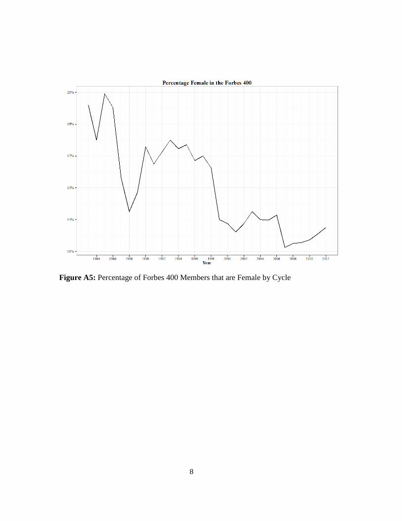
Figure A5: Percentage of Forbes 400 Members that are Female by Cycle

The Wealth Elasticity of Political Contributions by the...

Documents

Transcript of The Wealth Elasticity of Political Contributions by the...