THE VIABILITY OF A MARKET FOR

TRADABLE YIELD INDEX CONTRACTS FOR

AGRICULTURAL USE IN WESTERN AUSTRALIA

By Christopher Carter

B. Econs (Hons)

This thesis is presented for the degree of Doctor of Philosophy of The

University of Western Australia, School of Agricultural and Resource

Economics (Faculty of Natural and Agricultural Sciences)

June 2013

ii

iii

Abstract

Farms in the Western Australia wheatbelt are exposed to relatively high levels of

production risk. This thesis analyses the demand for traded derivatives based on

yield indices that can be used by farmers to hedge production risk. The volume of

demand by farmers is critical as it determines the long term viability of the yield

index contract.

This thesis contributes new knowledge by investigating how market design

influences farmers demand for a novel yield index contract that insures against

loss in poor grain production seasons. The thesis tests whether a market for

tradable yield index contracts in Western Australia is viable by simulating farmer

demand for the product in a range of designed markets.

The underlying yield indices for each market are specified according to the wheat

production characteristics in that region. The analysis investigates the effects of

alternate production characteristics, due to location, on farmers’ demand for

contracts.

Farmer demand is estimated using Monte Carlo simulation for a range of rainfall

patterns during the growing season. These simulated seasons are used as input

into a yield model and a valuation model to determine the price of (willingness to

pay for) the yield index contract contingent upon the seasonal conditions. Given

the price, transactions costs and the farmer’s current hedging ratio, a farmer

decides on adjustments to their hedging ratio. The estimates of traded volume

derived from the simulation provide an analysis of participation in the market and

expected transaction risk.

The results show that, even with an optimal contract specification, transaction

costs exclude all but the most risk averse farmers from participating in the

market. Given the constraints imposed by geographical basis risk, it is unlikely

that such a market would be viable without participation from a majority of

farmers in a region. This scenario is unlikely given the level of use of well-

established price futures markets.

iv

If the policy objective is to stabilise farm income through yield index contracts,

this can only be achieved by the injection of liquidity into the market from public

funds. As, based on the analysis here, the alternative purely free market solution

is not viable in the long run.

v

Contents

Abstract iii

Contents v

List of tables vii

List of figures viii

Acknowledgements x

Student Declaration xii

1 Introduction 1

1.1 Previous analysis 3

1.2 Research objectives and hypothesis 5

1.3 Thesis outline 5

2 Review of Literature on Insurance Demand 7

2.1 Relevance of utility theory to insurance demand 8

2.2 The demand for insurance 11

2.3 Pricing weather and yield index derivatives 16

2.4 Farmers’ decision making 20

2.5 Summary 22

3 Review of Literature on Weather Derivatives and Markets 25

3.1 Attributes of weather derivative markets and products 25

3.2 Construction of market and index 38

3.3 Summary 43

4 Western Australian agricultural Context 45

4.1 Farming in Western Australia 45

4.2 Summary 50

5 Construction of the Index, Contracts and market 51

5.1 Construction of an index for agricultural producers 51

5.2 Specification of the contract 57

vi

5.3 Construction of the market 59

5.4 Location of the representative shires 62

5.5 Weather and yield data 67

5.6 Summary 67

6 Rainfall, Yield and Price Modelling 69

6.1 Rainfall modelling 69

6.2 Yield modelling 72

6.3 Pricing the yield index contracts 76

6.4 Summary 78

7 Farmer Decision Making 79

7.1 The model of expected utility 79

7.2 Derivation of the hedge ratio 84

7.3 The simulation methodology 86

7.4 Summary 87

8 Results 89

8.1 Spatial differences in production and demand 89

8.2 Influence of market construction on farmers' participation in the

market 97

8.3 Viability of the proposed yield index contract 104

9 Conclusions 115

9.1 The effect of regional parameters upon demand 115

9.2 The effect of market construction upon demand 116

9.3 The viability of a market for yield index contracts 116

9.4 Further research 117

10 References 119

11 Appendix 1: Matlab Code 131

vii

List of tables

Table 5-1: Results of Regression analysis of the sum of rainfall based

index on yield in selected WA shires. 52

Table 5-2: R-Square values for functional forms of yield index 56

Table 5-3: Characteristics of representative shires used in this thesis 64

Table 6-1: Comparison of means (µ) and variance (σ) of observed and

simulated rainfall 72

Table 8-1: Expected net surplus/deficit ($/t) and standard deviation of net

surplus when farmers do not hedge. 90

Table 8-2: Probability that the farmers experience net deficit 90

Table 8-3: The initial contract price by shire and the initial contract price

as a percentage of the farmers expected net surplus 91

Table 8-4: CARA coefficients used in this thesis and the equivalent

CRRA coefficients 92

Table 8-5: Initial hedge ratio by shire for CRRA equivalent 92

Table 8-6: Comparison of expected utility for hedging and non hedging

strategies for Mullewa with CRRA = 1.06 100

Table 8-7: Detail on the alternative market constructions 101

Table 8-8: Difference in expected utility between using the given market

construction and a no hedging strategy 101

viii

List of figures

Figure 2-1: Expected utility of a risk averse agent 9

Figure 2-2: Effect of D and alpha parameters on V(μ) 13

Figure 5-1: Physical structure of the market for yield index contracts 60

Figure 5-2: Map of locations used in this study 65

Figure 5-3: Plot of Pearson correlation of shire yield and distance between

representative weather measuring points for five WA shires 66

Figure 6-1: Initial yield distribution for all shires 74

Figure 6-2: Final yield distributions for all shires 75

Figure 8-1: Expected Price of the yield index contract during the season, by

shire 91

Figure 8-2: a-j. Mean and spread of shire hedge ratios for different CRRA

coefficients 95

Figure 8-3: Distribution of hedge ratios for Mullewa when CRRA is 1.32 for

different weeks 95

Figure 8-4: Expected certainty equivalent of the hedging over the non

hedging strategy by shires and risk aversion 97

Figure 8-5: The cumulative distribution of utility with and without hedging at

week 20 for a farmer in Mullewa with a risk aversion coefficient of a)

1.06 and b) 2.38 99

Figure 8-6: Relationship between contract premium and the risk premium;

and contract premium and the supply of the contract to the market at

week 15, for two scenarios. a) Scenario 2: Farmer can change hedge

at any time b) Scenario 5: Farmer can change hedge at 5 week

intervals 104

Figure 8-7: Relationship between percentage increase of the non actuarial

premium and the initial hedge ratio for multiple coefficients of risk

aversion in the Mullewa Shire. 106

ix

Figure 8-8: Farmer offers in the market as a percentage of total unclosed

positions by initial fixed transaction cost 107

Figure 8-9: Probability of farmer changing hedge ratio for given weeks during

the season, by transaction cost premium. Data for Mullewa shire with

CRRA = 1.06 108

Figure 8-10: Number of interaction in the market for a range of additional

transaction costs. For Mullewa shire, CRRA 1.06 108

Figure 8-11: Number of interaction in the market for a range of additional

transaction costs. For Mullewa shire, CRRA 2.35 109

Figure 8-12: Non actuarial premium required by traders as a fee to enter

market due to transaction risk: market construction 4, Mullewa Shire,

Model run with no initial transaction risk premium 110

Figure 8-13: Non-actuarial premium required by traders as a fee to enter

market due to transaction risk: market construction 4, Mullewa Shire,

Model run with initial transaction risk premium of 30% 110

Figure 8-14: Effect of the transaction risk premium on the difference in the

farmers certainty equivalent in using the hedging and non-hedging

strategy in the market construction number 4 112

Figure 8-15: Effect of the transaction risk premium on the difference in the

farmers certainty equivalent in using the hedging and non-hedging

strategy in the market construction number 5 112

x

Acknowledgements

I would like to acknowledge the contributions of the Australian Research Council

(ARC) and the Department of Agriculture and Food Western Australia (DAFWA)

for providing the opportunity to undertake this research through an ARC Industry

Linkage Grant.

I would also like to say thank you to all the people who have encouraged,

supported, cajoled, pushed and pulled, harassed and sometimes dragged me on

the stop start journey I have travelled with this thesis.

Firstly to Ben White my supervisor for most of my study, who showed utmost

patience and commitment in support of my work.

To Greg Hertzler and Morteza Chalak, who played their parts at either end of this

process. To Greg, this would never have started without your efforts and

inspiration. To Morteza, I can't thank you enough for the effort you put in, in the

final months.

To Jo Pluske your positivity was a huge contributor to my continued progress, so

thank you.

Deb Swindells, Jan Taylor and Theresa Goh, thank you for all of your assistance

and support from the School of Agricultural and Resource Economics office.

A large part of my thanks go to Pete Metcalfe from DAFWA who was there at the

start and still there at the end, your support has always been hugely appreciated.

Many thanks to Shona Zulsdorf for spending much time and effort assisting with

reading, re-reading and supplying with cups of tea.

To the rest of crew at the Department of Agriculture and Food WA who provided

assistance with data and in the latter stages some healthy encouragement to

complete, again thank you.

Finally to my wonderful family, there is nothing I can write here that could convey

the way I have appreciated your unstoppable belief, your patience, your

encouragement and you just being there.

xi

For Shirin, you have been brilliant, enormous thanks for your patience and

support throughout the years.

For my gorgeous girls, Kiska and Zelia, the waiting is up, its time to put the boat

in the water and go for a sail.

xii

Student Declaration

This thesis does not contain work that I have published, nor work under

review for publication.

Student Signature .................................................................................................

Coordinating Supervisor Signature.

..……………………………………………………………………

1

1 INTRODUCTION

Adverse seasons are a serious risk to the long-term viability of farm businesses.

Potentially, multi peril crop insurance is a tool that farmers can use to reduce the

economic impact of adverse seasons (Hertzler 2005). A multi peril crop insurance

contract pays an indemnity to the farmer in an adverse season regardless of the

cause of the loss. In other words, the indemnity is paid whether the loss is due to

drought, frost, pests, disease or fire.

Governments subsidise multi peril crop insurance in both developing countries,

including Brazil and India (Skees, Hazell et al. 1999) and developed countries

United States and Canada (Skees, Hazell et al. 1999; Turvey 1999; Goodwin

2001; Vedenov and Barnett 2004; Hertzler 2005; Hertzler, Kingwell et al. 2006).

Historical precedence suggests that multi peril crop insurance is not viable

commercially, due to the costs associated with asymmetrical information,

specifically moral hazard and adverse selection (Miranda and Glauber 1997).

Moral hazard is defined as the capacity of the holder of an insurance contract to

change the nature of the insured risk once insured. Adverse selection occurs

where the one party holds additional information regarding the insured risk and

can use the information for economic benefit. The other significant historical

cause of poor performance in multi peril crop insurance is systemic risk. Systemic

risk occurs where there is significant temporal correlation between claims on the

same insurance policy by insured parties. The effect of systemic risk has become

less than historically recognised, with the development of a global underwriting

industry willing to absorb this cost.

The multi peril US Federal Crop Insurance Program in the United States has

experienced loss ratios in excess of 1.88 in the United States (Goodwin 2001).

Despite these losses, federal or provincial governments in the United States and

Canada continue to subsidise multi peril crop insurance. Farmers in Australia do

not have state or federal government subsidised multi peril crop insurance

schemes (PC 2009; OECD 2010). The federally based national drought policy

supports farm businesses to prepare for adverse seasonal conditions through

2

strategic planning, and does not support the ex-post remuneration of farmers for

poor seasons. As there is minimal government support measures in Australia,

government policy does not crowd out commercial production insurance products

for farmers (Hertzler 2005).

While traditional multi peril crop insurance cannot be designed without

asymmetrical information, a index based insurance, can reduce or eliminate

these problems (Miranda and Glauber 1997; Skees, Hazell et al. 1999; Turvey

2001). Index insurance uses an index that is highly correlated with revenue in the

target industries. The value of the index relative to an exercise/ strike price

determines the indemnity paid. This is different to an assessed insurance where

the insurer pays an indemnity once the actual loss of the business has been

assessed (Turvey 2001). In agriculture, the forms of index insurance most likely

to be successful are weather and yield index contracts (Hertzler, Kingwell et al.

2006).

Weather derivatives are contracts drawn on a weather based underlying variable

(Hao, Kanakasabai et al. 2004; Jewson and Brix 2005; Musshoff, Odening et al.

2006). Hertzler specifies the difference between a weather derivative and a

financial derivative as where

“[t]he underlying variable is not a price but a quantity such as millimetres of

rainfall" (Hertzler 2004 p.1)

A yield index derivative is where the underlying is an index of expected yield. A

market maker or independent authority uses a crop yield model that incorporates

seasonal conditions to model the expected yield from the observed weather

conditions.

Weather derivatives have potential as a tool to manage seasonal risk in

agriculture. The type of risk that a derivative product can manage are where

payouts are highly spatially correlated, regular and often small. Insurance is more

appropriate for low probability of occurrence and little correlation in the timing of

claims (Yoo 2003).

3

1.1 Previous analysis

The viability of multi peril crop insurance has been subject to a broad empirical

and theoretical literature in agricultural economics. Bardsley et al. (1984) use a

model of supply and demand for crop insurance to determine the potential for a

crop insurance scheme in Australia. They conclude that there is no prospect for

an unsubsidised crop insurance scheme in Australia on the basis that the farmer

gains relatively little utility from taking out a contract and therefore demand will be

insufficient to support the market.

Quiggin (in a reply to Bardsley et al.) questions the assumption of their paper

especially the measure of risk aversion of the insurer (Quiggin 1986). Quiggin

concludes that there is potential for a crop insurance market if insurers are risk

neutral and combine the crop insurance with non-correlated assets in a portfolio.

In response, Bardsley states that there may be a viable model though farmers

would only use the insurance to cover a small proportion of crop risk (Bardsley

1986).

Since the debate between Bardsley and Quiggin there have been few analyses

of the viability of crop insurance for Australia outside of government

commissioned reports. Of these reports several specifically relate to multi peril

crop insurance in Western Australia see (Industries Assistance Commission

1996; Ernst and Young Consultants 2000; Collinson 2001; Ernst and Young

Consultants 2003). These reports conclude that multi peril crop insurance is not a

viable commercial product in Western Australia as the product would suffer from

asymmetrical information and systemic risk.

Ernst and Young (2003) recommend that there is potential for weather derivatives

in the absence of multi peril crop insurance and a drought safety net. Hertzler

(2004) designed a framework for the pricing of a yield index contract for

Australian conditions. Hertzler derives a quantifying equation to "price" a yield

index contract though stops short of determining whether there would be demand

for such a product.

The earliest use of weather derivatives was in the American energy industry in

1997 (Considine 2005). The development of these products started due to

concern over the predictions for a strong El Nino effect in 1997-98. In the energy

industry, an underlying based on either extremely cold or hot days can be highly

4

correlated with power generation costs. The contracts derived from this type of

index removes some of the weather related risk for the industry. These exchange

traded contracts have been highly successful in terms of volumes with weather

derivatives now available for many of the major cities in the US, Asia, Europe and

Australia. There are however, significant differences in the design of an

accumulative index for the energy industry and the design of an index that is

applicable to agricultural production risk.

The current literature does not analyse farmer demand for tradable yield index

derivative contracts, henceforth referred to as yield index contracts, supplied

through a market exchange. This type of product is new to the literature and is

not available in Australia, and to the best of knowledge, these products are not

currently available to agricultural producers. In this model of the market, yield

index contracts would be subject to low transaction costs and there is a risk

neutral supplier of contracts, through an exchange market. This form of market

reduces concerns of moral hazard and systemic risk that exist in traditional

insurance markets. Farmer demand in a market for a yield index contracts, have

not been analysed. This thesis addresses this gap in the literature. It also extends

a static model of farmer demand for insurance into a multi-period analysis, where

farmers can trade on a secondary market for yield index contracts. This thesis

uses a whole market approach to identify if there are structural weaknesses in

the contract design that affect farmers participating in the market, and thus

market viability.

This thesis uses a Monte Carlo methodology to simulate trades within a yield

index contract market. Sustained market volumes during the life of the contract

maintain prices at close to the actuarial premium (the expected value of a

contract) by a competitive process. Where the market volumes are not sustained,

market makers charge a risk premium above the actuarial rate. The thesis

determines whether demand by risk averse farmers for yield index contracts at

premia above the actuarial rate is sufficient to maintain market viability.

5

1.2 Research objectives and hypothesis

This thesis contributes new knowledge by investigating how market design

influences farmers demand for a novel yield index contract that insures against

loss in poor production seasons. The thesis evaluates whether a market for

tradable yield index contracts in Western Australia is viable. To the best of the

author's knowledge, there are no yield index contracts with an active secondary

market. While there is a substantial literature on the supply of similar contracts,

there have been few studies of demand for yield index derivatives for broad acre

cropping, and none that assess how market design affects demand for the

product.

This research explores whether market design for yield index contracts is a

significant determinant of the viability of the market. Specifically it is hypothesised

that the preference for yield index contracts dominates not using yield index

contracts at low to moderate levels of risk aversion. If this hypothesis is true, the

study will address a second hypothesis that the preference for the contracts

would generate sufficient demand to establish a viable market.

1.3 Thesis outline

Chapter 2 presents the theoretical models relevant to this study. These models

include the standard utility theory, the model of demand for insurance and option

pricing methodology.

Chapter 3 reviews the state of the literature on weather derivatives and the how

the markets for weather derivatives are constructed.

Chapter 4 describes the Western Australia broad acre cropping sector in terms of

production characteristics and agricultural policy. This chapter includes a

discussion of the data used in the thesis.

Chapter 5 analyses the design of yield index contracts and the pricing of the

contracts. This chapter includes the description of the data for the simulation

model and the simulation of weather and yield data.

Chapter 6 presents the methodology used to simulate the weather, which is used

to create a yield index. The pricing methodology is based on the yield index.

6

Chapter 7 presents the decision making model. The chapter develops the

methods to determine the hedging decision in a myopic hedging strategy. The

chapter defines the farmers' utility functions and payoffs, and incorporates a

production hedge into the payoff. The chapter develops the model to analyse the

demand for yield index contracts.

Chapter 8 shows results based on the analysis of the model described in

chapters 6 and 7 and assesses market viability.

Chapter 9 summarises the conclusions of the thesis and state whether the results

confirm the hypothesis, and discusses further research.

7

2 REVIEW OF LITERATURE ON INSURANCE DEMAND

'There would be no risks if there were no uncertainties, though there may be

many uncertainties without any risk being taken' (Kast and Lapied 2006 p.85)

Finance formalises risk analysis based on the parameters of the underlying

random variable (Buhlmann 1970; Merton 1990; Oksendal 1992; Moix 2001;

Melinikov 2004). The parameters of the random variable determine the expected

distribution of returns and the expected value of the investment decision. In

agriculture there is a high degree of uncertainty in production due to the large

number of uncertain factors that affect production (Anderson, Dillon et al. 1977).

However, the principles of risk used in finance are still apply (Kingwell, Pannell et

al. 1993).

A farmer manages multiple risks including production risk, input and output price

risk, business risk, counterparty risk and personal risk (Hardaker, Huirne et al.

1997; Skees, Hazell et al. 1999). Production risk and price risk are the most

significant risks to the viability of the farm. To manage these risks, producers can

use price-hedging mechanisms through futures and forward contracts, and

named peril (hail and fire) insurance. In the United States and Canada farmers

have access to multi peril crop insurance.

In countries with subsidised insurance, the level of subsidy is adequate to

generate sufficient demand to ensure the product is viable for the insurer. In

Australia, crop insurance is not subsidised and the demand for insurance is

based on how the farmer perceives the effect of insurance on their utility. To

understand the demand for production insurance, we need to first understand the

theory regarding decision making between risky alternatives.

This chapter presents the theory that is most relevant to this study. The theory

informs the empirical analysis of this thesis. The theory included in this chapter

includes the expected utility theory and the theory of insurance demand. There is

8

additional discussion on the pricing of weather derivatives and farmer decision

making, as applied in this study.

2.1 Relevance of utility theory to insurance demand

"Expected utility models are concerned with choices between risky prospects

whose outcomes may be single or multi dimensional". (Schoemaker 1982 p. 530)

Von Neumann and Morgenstern (1944) developed the most widely used model of

decision making under uncertainty, the expected utility theory. The theory is

constructed based on three axioms, being transitivity, reflexivity, and

completeness, that inform decision making under risk (Von Neumann and

Morganstern 1953). Neumann and Morgenstern discuss the role of the agents

preferences when constructing the axioms of utility. They state that it is not

possible to develop axioms of choice to explain gambling without introducing

contradictions. The importance of the human perception of risk to a decision

making model is a common theme running through the utility literature. It arises in

all the main theoretical developments including rank dependency, subjective

expected utility, and cumulative prospect theory.

Friedman and Savage (1948) state that the curvature of the utility function,

defined by the second derivative of utility with respect to wealth, would affect how

the decision maker would act. Where the curvature of the utility function is

concave to the origin, the utility of the expected value of the fair odds gamble are

greater than the utility of the gamble. The decision maker would prefer a small

loss to ensure a certain income than choose the risky gamble. This defines the

preference of a risk averse individual. Where the utility function in convex to the

origin, the opposite applies; the agent is willing to pay a small price to take the

risky gamble rather than the certain outcome. Friedman and Savage introduced

the risk aversion and risk seeking terms into common use. The concept of risk

aversion is critical to the demand for insurance, where an agent must forego an

amount with certainty to ensure a less risky return. The basic structure of the

expected utility theory, with a risk averse agent is presented in Figure 2-1.

9

Figure 2-1: Expected utility of a risk averse agent

In Figure 2-1, points a and b represent the two possible outcomes of a gamble,

where the odds of each outcome are 0.5. The expected value of a gamble is

point w1 where,

baw2

1

2

11 (2.1)

And the utility from the expected value of the gamble is U1, where

11 wUU (2.2)

However, the utility from the gamble U2 is

bUaUU2

1

2

12 (2.3)

For this level of utility, the agent is willing to forego P, the value of

21 wwP (2.4)

to receive a certain return of w2 in Figure 2-1, instead of the fair odds gamble for a

and b. In (2.4), w2 is the value of the certainty equivalent of the gamble. The

certainty equivalent is the value of the gamble to a risk averse decision maker. P

is the risk premium and w1 is the expected value of the gamble. It is easy to see

that the certainty equivalent plus the risk premium is equivalent to the expected

return of the gamble.

Wealth

Uti

lity

WW

b

a

U1

U2

c

d

2 1

10

The expected utility and rank dependency type forms are the two dominant

approaches used to determine the utility for a decision maker (Schoemaker

1982). The rank dependency forms have had limited applications to farm decision

making (Serrao and Coelho 2004). The rank dependency model is less widely

used than the expected utility model despite the failure of expected utility model

to predict individual choices. Bar Shira (1992) and Hardaker et al. (2003)

conclude that the expected utility model provides an adequate prediction of

decision making. In this study the expected utility model is used, despite its

limitations a predictive model, in a normative model of producer risk preferences.

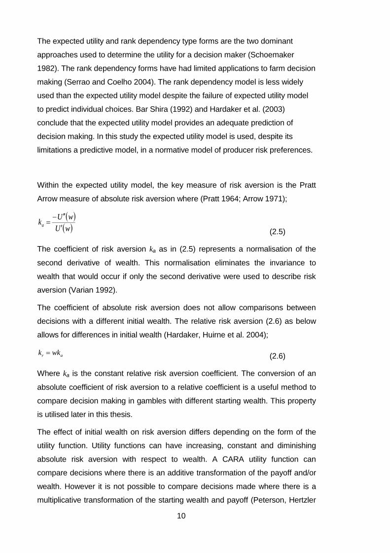
Within the expected utility model, the key measure of risk aversion is the Pratt

Arrow measure of absolute risk aversion where (Pratt 1964; Arrow 1971);

(2.5)

The coefficient of risk aversion ka as in (2.5) represents a normalisation of the

second derivative of wealth. This normalisation eliminates the invariance to

wealth that would occur if only the second derivative were used to describe risk

aversion (Varian 1992).

The coefficient of absolute risk aversion does not allow comparisons between

decisions with a different initial wealth. The relative risk aversion (2.6) as below

allows for differences in initial wealth (Hardaker, Huirne et al. 2004);

(2.6)

Where ka is the constant relative risk aversion coefficient. The conversion of an

absolute coefficient of risk aversion to a relative coefficient is a useful method to

compare decision making in gambles with different starting wealth. This property

is utilised later in this thesis.

The effect of initial wealth on risk aversion differs depending on the form of the

utility function. Utility functions can have increasing, constant and diminishing

absolute risk aversion with respect to wealth. A CARA utility function can

compare decisions where there is an additive transformation of the payoff and/or

wealth. However it is not possible to compare decisions made where there is a

multiplicative transformation of the starting wealth and payoff (Peterson, Hertzler

wU

wUka

ar wkk

11

et al. 2000) using this utility function. One advantage of a utility function with

CARA is that it allows for negative payoffs (Peterson, Hertzler et al. 2000).

Newbury and Stiglitz (1981) state that the CARA utility function is

“Useful for solving portfolio problems such as the choice of a hedge in a futures

market” (Newbery and Stiglitz 1981)

Binswanger (1981) estimates the risk aversion of farmers in India. Binswanger

uses a methodology where the farmers are invited to participate in a series of

gambles with increasing returns. In the study, farmers participate in three rounds

of decisions over a period of six to eight weeks. In each round of decisions, the

value of the gamble increases by a multiple of ten. The farmers are offered the

choice between a set of gambles where the expected value of the gamble

increases as the variance of the gambles increase. The finding is that the farmers

commonly hold a risk aversion that is neutral to intermediate for small gambles,

and moderate to severe for large gambles. This study finds that there is a

tendency, as the value of the gamble increases, to see a leftwards shift in the

distribution of risk aversion. The study also finds that the value of the gamble

itself has more influence on the decision making process than the total wealth

following the gamble.

Bond and Wonder (1980) state that while the average degree of risk aversion is

low in farmers, there is a wide distribution that highlights the need to use a

distribution of risk aversions when modelling farmer decision making.

The CARA expected utility function is used extensively in the literature

investigating the demand for insurance (Newbery and Stiglitz 1981; Simmons and

Rambaldi 1997). The widespread application of the CARA expected utility

function applied analysis justifies its application here though following on from

Bond and Wonder (1980) the study must use a distribution of risk aversion

coefficients.

2.2 The demand for insurance

An insurable risk is one that is not prone to asymmetrical information, where the

insured event is measurable and the measurement determines the indemnity

paid (Eeckhoudt and Gollier 1995).

12

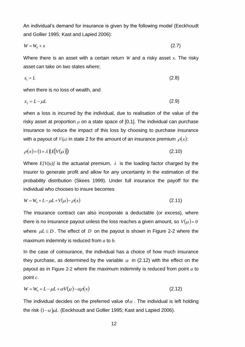
An individual’s demand for insurance is given by the following model (Eeckhoudt

and Gollier 1995; Kast and Lapied 2006):

xWW 0 (2.7)

Where there is an asset with a certain return W and a risky asset x. The risky

asset can take on two states where;

Lx 1 (2.8)

when there is no loss of wealth, and

LLx 2 (2.9)

when a loss is incurred by the individual, due to realisation of the value of the

risky asset at proportion μ on a state space of [0,1]. The individual can purchase

insurance to reduce the impact of this loss by choosing to purchase insurance

with a payout of V(μ) in state 2 for the amount of an insurance premium x :

VEx 1 (2.10)

Where E[V(u)] is the actuarial premium, is the loading factor charged by the

insurer to generate profit and allow for any uncertainty in the estimation of the

probability distribution (Skees 1999). Under full insurance the payoff for the

individual who chooses to insure becomes

xVLLWW 0 (2.11)

The insurance contract can also incorporate a deductable (or excess), where

there is no insurance payout unless the loss reaches a given amount, so 0V

where DL . The effect of D on the payout is shown in Figure 2-2 where the

maximum indemnity is reduced from a to b.

In the case of coinsurance, the individual has a choice of how much insurance

they purchase, as determined by the variable in (2.12) with the effect on the

payout as in Figure 2-2 where the maximum indemnity is reduced from point a to

point c.

xVLLWW 0 (2.12)

The individual decides on the preferred value of . The individual is left holding

the risk L1 (Eeckhoudt and Gollier 1995; Kast and Lapied 2006).

13

Figure 2-2: Effect of D and alpha parameters on V(μ)

The utility function with insurance is (2.13).

dfLVLLwUwUE

1

0

12 1 (2.13)

The first derivative of utility with respect to identifies the demand for insurance

(Eeckhoudt and Gollier 1995). Where is E , to take the derivative of this

function we derive

01

1

0

22

dfLwU

d

wUdE (2.14)

Given that

LCLLwxw 112 (2.15)

This thesis uses these functions to derive the demand for insurance. The demand

function incorporates the coinsurance coefficient, though not the deductible

constraint. The thesis shows how the demand for insurance changes over time,

and subsequently affects the viability of the market for yield index contracts for

agricultural use.

2.2.1 Agricultural insurance

Agricultural insurance and hedging agricultural risk is not a new concept: Farmers

have used forward contracts since the Meiji era (1600's) in Japan to set forward

Loss

Ind

em

nit

y .

V(μ)

μL

αV(μ)

V(μ)-D

d0

a

c

b

14

prices for rice (Bernstein 1996). In some countries the insurance industry has

offered farmers multi peril crop insurance, to provide farmers with a tool to

manage production risk (Miranda and Glauber 1997; Skees 1999; Turvey 1999;

Collinson 2001; Vedenov and Barnett 2004; Hertzler, Kingwell et al. 2006).

The literature on multi peril crop insurance is extensive (Bardsley, Abey et al.

1984; Quiggin 1986; Miranda and Glauber 1997; Richards 1998; Turvey 2001;

Sherrick, Barry et al. 2004) and not entirely in agreement on the key issue of

market viability. The consensus holds that multi peril crop insurance is not

commercially viable (Miranda and Glauber 1997; Goodwin 2001; Sherrick, Barry

et al. 2004; Hertzler 2005). An insurance product with an indemnity premium ratio

(the ratio of the total cost of offering an insurance product, including

administration costs and indemnities paid out by an insurer to the premiums

received) less than 1 is a viable product and a ratio in the range of 0.88 to 0.95

allows a commercial return (Skees 2010). Goodwin (2001) states that the true

historical indemnity to premium ratio is 1.88 for American multi peril crop

insurance products. This ratio indicates that the scheme would not be

commercially viable and is consequently underwritten by US Government (Skees,

Hazell et al. 1999).

Despite this finding, the US multi peril crop insurance is one of the more

successful schemes when compared to other available or previously available

schemes in other countries. The US scheme exhibits one of the lowest indemnity

premium ratios. Skees and Hazell (1999) state that the indemnity premium ratio

of Multiperil crop insurance in other countries ranged from 2.60 in Japan to 5.74

in the Philippines with all the MCPI programs heavily subsidised by the

government.

Typically, asymmetric information undermines the commercial viability of crop

insurance, where one participant in the market (usually the farmer) has more

information than the other (the insurance company) and the information can be

used to extract rent.

Asymmetrical information can be further decomposed into moral hazard and

adverse selection (Akerlof 1970). Adverse selection is a leading cause of non-

viability of the U.S crop insurance market (Goodwin 1993; Miranda and Glauber

15

1997; Turvey 1999; Collinson 2001; Goodwin 2001; Sherrick, Barry et al. 2004;

Vedenov and Barnett 2004; Ginder and Spaulding 2006). Adverse selection

occurs when high risk farmers purchase insurance at the same price as the low

risk farmers. In crop insurance markets, this means there are a higher proportion

of high risk farmers in the insurance pool than in the general farm population. The

high risk farmers make more claims on the insurance while paying premiums that

are lower than the actuarial price for the risk in their individual contracts. If the

price of insurance increases to the actuarially fair premium for the high risk

farmers, there is a greater incentive for the low risk farmers, who are not likely to

claim, to reduce their level of insurance (Goodwin 2001).

Moral hazard in insurance is the over reporting of losses, or the under reporting of

risks (Varian 1992). Either of these actions by the insured leads to sure losses to

the insurer in the long term, as the premiums do not cover actual indemnities. In

the long run, moral hazard leads to either actuarially unfair premiums, or the

breakdown of the insurance market (Varian 1992) . Moral hazard is a significant

cause of non-viability of multi peril crop insurance (Goodwin 1993; Vedenov and

Barnett 2004).

Systemic risk is another significant cause of non viable crop insurance markets.

Systemic risk occurs where there is a high correlation in the timing of insurance

claims. Kaufman and Scott (2003) define systemic risk using a definition for the

banking sector that is equally applicable in the insurance sector.

“Systemic risk refers to the risk or probability of breakdowns in an entire system,

as opposed to breakdowns in individual parts or components, and is evidenced

by comovements (correlation) among most or all the parts” (Kaufman and Scott

2003 p. 371)

Skees defines systemic risk in relation to crop insurance as “low frequency high

consequence loss events that are correlated across space” (Skees and Barnett

1999).

Systemic risk in agricultural insurance occurs where there is high spatial

autocorrelation in farm production, which means insurers cannot reduce risk by

creating a larger portfolio within a region (Miranda and Glauber 1997). Spatial

autocorrelation occurs when the probability of an insurance claim in one region

displays a correlation with the adjacent spatial region. This correlated risk

16

increases the likely indemnity per unit of premium to higher levels than for other

business insurance (Miranda and Glauber 1997).

Miranda and Glauber (1997) state that for an efficient insurance industry the risks

should be independent across insured individuals. This is not the case for

agricultural insurance, where "crop losses display a substantial degree of

correlation across space" (Miranda and Glauber 1997). Where there is systemic

risk the coefficient of variation of indemnities for the US crop insurance schemes

ranged from 67% to 130% . If the indemnities were independent as would occur

in a more traditional insurance market, the coefficient of variation of total

indemnities would be in the order of 1 to 4% (Miranda and Glauber 1997).

Miranda and Glauber (1997) state that asymmetric information is a lesser cause

of failure in the crop insurance market than systemic risk however it is difficult to

separate the effects of these two problems.

While traditional multi peril crop insurance cannot be designed without

asymmetrical information and systemic risk, an index based insurance, can

reduce or eliminate these problems (Miranda and Glauber 1997; Skees, Hazell et

al. 1999; Turvey 2001). Index insurance uses an index that is highly correlated

with revenue in the target industries. The value of the index at the maturity of the

contract, relative to an exercise/ strike price determines the indemnity paid. This

is different to an assessed insurance where the insurer pays an indemnity once

the actual loss of the business has been assessed (Turvey 2001). In agriculture,

the forms of index insurance most likely to be successful are weather and yield

index contracts (Hertzler, Kingwell et al. 2006).

2.3 Pricing weather and yield index derivatives

Index insurance is analogous to purchasing an option to sell stock in an

exchange market (put option). To derive the premium for the index insurance

there are similarities with the option pricing methodology developed by Black and

Scholes (Black and Scholes 1973) and Merton (Merton 1973). Before 1973 the

attempts at creating an equilibrium pricing model were unsatisfactory (Cox, Ross

et al. 1979). Black and Scholes (1973) presented a method to calculate the

option price utilising the diffusion process of the asset price to determine the

probability of a stock exceeding a particular strike price. The price of the hedge

17

and the optimal hedge ratio replicated the payoff function of the underlying. This

method limited opportunities for arbitrage, though assumed the contract could be

traded continuously without transaction costs. Merton (1971) used a similar

calculation and the same formula was revealed independently of Black and

Scholes. Merton (1973) extends the Black and Scholes formula to include the

payment of dividends from an underlying stock. As agricultural derivatives are a

form of option, it is reasonable to expect that the pricing methodology borrows

heavily from the option pricing methodologies.

Hertzler outlines the inherent difficulty in pricing a yield index derivative. “Instead

of observing an option price and choosing the quantity for their portfolio, a farmer

observes the option quantity and chooses the price” (Hertzler 2004)

As an example, a farmer may purchase a yield index contract that provides a

payout in a poor season. When purchasing the product, the farmer nominates a

strike price and a value, or tick. The strike price indicates the value of production

below which the farmer receives an indemnity. The tick price is the value per unit

increment of the index, in the case of a yield index product the tick would be the

price per . The tick ensures the marginal return on the insurance indemnity is the

same as the marginal loss in revenue. However, in the case of index insurance,

this creates an incomplete market, as traders are not able to trade the underlying,

as it is an index. There is also no possibility for arbitrage, which means that

traditional risk neutral pricing tools cannot be used (Hertzler 2004).

The complication in pricing leads to premiums for yield and weather index

contracts that are higher than the actuarial price that would be expected for the

same product where there is an asset with a replicating payoff. The supply side of

the market errs on the side of caution and increase the premiums to offset any

uncertainty in their initial pricing (Skees 2010). This occurs as the insurers cannot

adequately price the uncertainty and make a best guess as to its value.

The most promising methods for pricing weather derivatives are numerical

methods. Xu uses an indifference pricing method to determine the price of

weather derivatives in Germany, where the price is determined by the willingness

of a weather exposed industry to pay for the derivative (Xu, Odening et al. 2007).

This methodology identifies the price at which the purchaser is indifferent

between buying and not buying the derivative. This price sets an upper limit on

18

the price of the derivative above which there is no demand for the product. The

indifference pricing method assumes the ability to determine the utility of

participants in the market, and may be suited for an over the counter style

market. One of the findings of the study is that even with moderate coefficients of

risk aversion there are few locations where the bid by farmers would have been

above the offer price of most product suppliers. This is supported through other

literature, mostly from the multi-peril crop insurance literature, where there is an

general lack of demand to cover weather risk at the market rate (Simmons and

Rambaldi 1997; Ernst and Young Consultants 2000; Simmons 2002; Considine

2005)(East 2006).

Alaton et al. (2002) use two methods to determine the price for weather

derivatives for the energy industry. The first method is a functional approach,

while the second method uses a Monte Carlo simulation. The functional approach

assumes a normal distribution for the outcomes of an energy industries weather

derivative. The prices generated by the two methods were similar, within 2 per

cent of each other for three option contracts.

Musshoff et al. (2006) investigates three methods of pricing weather derivatives;

a burn analysis; an index value simulation; and a daily simulation. The burn

analysis uses historical data to provide the distribution of returns and assess the

probability and impact of losses. The index simulation uses empirical data to

derive a parameterised weather distribution from which a selection of seasons

could be sampled. The daily simulation methodology uses estimates of daily

rainfall probabilities, with the expected distribution of returns derived from

observations from the rainfall simulations. The paper concluded that each of the

methods has advantages, with the daily specification index providing smaller

confidence intervals than the burn analysis though with greater potential for mis-

specified parameters.

For agriculture the pricing of the options is more suited to a numerical approach.

Hertzler (2004) approaches a pricing methodology using a chain rule method.

The methodology followed by Hertzler to get to the differential of price for the

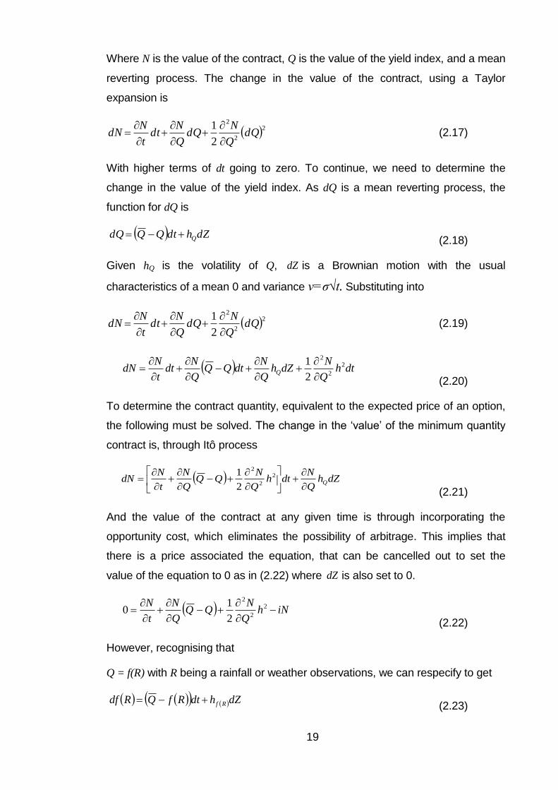
yield index contract is followed below, starting with;

tQfN , (2.16)

19

Where N is the value of the contract, Q is the value of the yield index, and a mean

reverting process. The change in the value of the contract, using a Taylor

expansion is

22

2

2

1dQ

Q

NdQ

Q

Ndt

t

NdN

(2.17)

With higher terms of dt going to zero. To continue, we need to determine the

change in the value of the yield index. As dQ is a mean reverting process, the

function for dQ is

(2.18)

Given hQ is the volatility of Q, dZ is a Brownian motion with the usual

characteristics of a mean 0 and variance v=σ√t. Substituting into

22

2

2

1dQ

Q

NdQ

Q

Ndt

t

NdN

(2.19)

(2.20)

To determine the contract quantity, equivalent to the expected price of an option,

the following must be solved. The change in the ‘value’ of the minimum quantity

contract is, through Itô process

(2.21)

And the value of the contract at any given time is through incorporating the

opportunity cost, which eliminates the possibility of arbitrage. This implies that

there is a price associated the equation, that can be cancelled out to set the

value of the equation to 0 as in (2.22) where dZ is also set to 0.

(2.22)

However, recognising that

Q = f(R) with R being a rainfall or weather observations, we can respecify to get

(2.23)

dZhdtQQdQ Q

dthQ

NdZh

Q

NdtQQ

Q

Ndt

t

NdN Q

2

2

2

2

1

dZhQ

Ndth

Q

NQQ

Q

N

t

NdN Q

2

2

2

2

1

iNhQ

NQQ

Q

N

t

N

2

2

2

2

10

dZhdtRfQRdf Rf

20

Where

(2.24)

(2.25)

Using the Itô process,

(2.26)

Introducing into equation (2.21) we get

(2.27)

At this point, it is evident that the solution of the price is not achieved analytically.

The nonlinear transform of the random variable becomes intractable. This leads

into the approach for the rest of the thesis where numerical methods are used to

determine the pricing.

This thesis uses the burn analysis method outlined in Musshoff et al. (2006). To

use the burn analysis we need to use a distribution of historical data. As this

thesis uses a market that permits the inter-seasonal trading of agricultural

derivatives, it also needs to generate the data for the burn analysis. Conventional

historical data does not contain the yield expectations at all times during the

season, only the yield results at the end of the season. We firstly need to provide

data that allows the daily simulation of rainfall and derivation of yield then price

from this simulated data.

2.4 Farmers’ decision making

The farmers' decision making process determines the level of participation in the

market for insurance and yield index contracts. These decisions include the

estimation of the optimal hedge ratio and the irreversibility of the decision.

dZhdR R

dRR

fRdf

dZhR

Rfdth

R

RfRdf RR

2

2

2

2

1

dZhdZh

R

Rfdth

R

RfdtRfQdQ RfR

2

2

2

2

1

21

2.4.1 Hedge ratios

The optimal hedge of an asset with an uncertain return occurs where the change

in the value of the hedge position replicates the change in value of the underlying

stock. Black and Scholes (1973) derive a hedge ratio that replicates the value of

an underlying asset if continuously updated. This strategy only works where there

are no transaction cost, otherwise the hedger faces near infinite transaction costs

(Albanese and Tompaidis 2008). A market for agricultural derivatives incurs

transaction costs. A weather derivatives market is incomplete so traditional

methods used to determine the optimal hedge ratio, such Black and Scholes

method, cannot be used.

Lapan and Moschini (1994) present a method to determine the hedge ratio for a

farmer exposed to price and production risk. In their paper they specify optimal

price hedge ratios for farmers with uncertain production and basis risk. Their

finding that a futures market for price hedging cannot create a perfect hedge

where there is uncertainty in production. The optimal hedge under these

conditions is a function of the decision makers risk aversion, the coefficients of

variation of price and yields, the volatility of the futures price and the bias of the

market amongst other variables. Their findings show that the optimal hedge

changes with time, depending on forecasts, and is sensitive to risk aversion.

Simmons solves a model of hedging, where the production decision and hedging

decision are made simultaneously. Based on Kahl (1994) the hedge ratio is a

function of the futures price, transaction costs, and the expected bias in the

market. The form of the function means there is a reduction in the hedge ratio as

there is increasing transaction costs. The results of the model show that even

with a low level of transaction costs, the demand for the hedging product from

farmers is very low.

2.4.2 Irreversibility

The purchase of insurance is regarded as an irreversible decision. When a

farmer has purchased the insurance, the contract is in place for a set period of

time. With respect to crop insurance, the farmer accepts the initial cost of the

insurance, and does not have any flexible options in managing the contract.

Within a derivatives market, the farmer has options to increase the hedge ratio,

decrease the hedge ratio or completely close the insured position. These

22

management options provide the farmer with some flexibility, and the flexibility

has a value (Trigeorgis 1993).

Where it is assumed that the farmer is myopic there is a threshold value at which

the decision to change hedge position is preferred. As the hedge is not fixed as in

an insurance contract, there is an option to wait and resolve uncertainty over the

value of the option and the underlying index (Dixit and Pindyck 1994). When

uncertainty is resolved, the farmer may make a decision to pay a premium for a

different expected income distribution at time T by changing the hedge position.

Creating a threshold influences the preferred hedging strategy for the farmer as

in Karp (1988) and Hanemann (1984).

2.5 Summary

This chapter has reviewed the standard model of utility theory and discussed how

the model can be applied in an empirical study. This discussion concluded that

the model of expected utility with constant absolute risk aversion framework

would be used for this study.

The demand for insurance model based on Eeckhoudt and Gollier (1995)

discussed in this chapter provides the framework used in this study. When

applied to agricultural insurance this framework encounters two problems, of

systemic risk and asymmetrical insurance. These problems have the potential to

reduce the viability of the market. To counteract the effects, it is possible to

change the method used determine an indemnity, from an assessment based

method to a parameter based method.

This chapter has shown that pricing of the index insurance is analogous to pricing

options to purchase stocks in the exchange markets. There are however

complications in pricing the weather derivatives for agriculture, through non linear

payoff functions. For this reason the approach we take, uses a numerical method

to find the price of the yield index contracts.

When a farmer purchase index insurance, they purchase what is the optimal

hedge ratio, given that purchasing insurance is an irreversible, risky decision from

which they experience economic consequences. The method a farmer uses to

determine the economic consequences, affects their participation in a market.

23

Given that farmer participation is one of the key drivers of market viability, the

model of farmer decision making is a key component of this study.

24

25

3 REVIEW OF LITERATURE ON WEATHER

DERIVATIVES AND MARKETS

This chapter reviews the current literature on markets for weather derivatives.

This review extends to the microstructure of the markets and the factors that

influence market viability. This facilitates discussion in following chapters of how

the market for yield index contracts needs to be designed.

3.1 Attributes of weather derivative markets and products

An alternative to using traditional insurance to hedge agricultural production risk

is to use weather and/or yield index derivatives. Weather derivatives [for

agriculture] are designed to hedge the volumetric risk associated with

unfavourable weather (East 2005). They are a type of index whose payoff

depends on occurrence or non-occurrence of specific weather events (Vedenov

and Barnett 2004) and are designed to hedge against risks of too little or too

much rainfall and high or low temperatures” (Hertzler 2004). Most importantly,

weather derivatives are financial instruments that allow market participants to

trade weather related risks (Musshoff, Odening et al. 2006). A yield index

derivative allows farmers to use a variant on the financial put or call option to

reduce the downside risk of crop production (Hertzler 2005).

Options are financial derivatives that allow agents to limit the downside risk of

holding an asset, while maintaining an upside risk (Merton 1973; Merton 1990;

Zhang 1998). They give an agent the option to purchase (call) or sell (put) an

asset at a fixed price at a time in the future (maturity). If the actual price of the

asset is above (call) or below (put) the fixed price, the holder of the option

contract exercises the option and collect the difference between the fixed and

actual price of the asset. (Cox, Ross et al. 1979; Geman 1999).

Weather derivatives for agriculture provide a risk management product with a

payoff similar to a financial option (Skees 2001). The payoff from a weather

derivative is based on the value of a parametric weather index called the

26

'underlying'. As an example, a farmer could purchase a weather derivative based

on an index derived from rainfall. The derivative contract would pay the farmer an

indemnity if the total rainfall were below a given quantity at the end of the season

(Skees, Hazell et al. 1999). If the index were below the strike price at the

expiration date of the contract the farmer could exercise the option and would

receive an indemnity. Where an index is highly correlated with farm production,

the indemnity would be similar to the revenue shortfall incurred due to the

weather (Skees, Hazell et al. 1999). It is important that the index that the farmer

uses to hedge production is highly correlated with revenue (Alaton, Djehiche et

al. 2002).

To increase the correlation between the underlying index and agricultural

production, one method is to create a yield index that is a function of multiple

weather variables. A yield index is a more efficient index than a weather variable.

The definition of an efficient index is an index that has a high correlation with the

efficient yield level. In other words, it provides indemnities in years where the

efficient yield is below the expected yield for a region. The design and

parameterision of a yield index determines the distribution of indemnity payments

to farmers (Hertzler 2004).

In agriculture, there is a lag of up to six months between the weather event, the

indemnity payment based on the yield index and the realised yield at harvest. In

WA, for instance, cereal crops are planted in autumn (April to May) and

harvested in summer November to January. Critical to the construction of a yield

index, a similar weather event, for instance a rainfall event, occurring at different

times of the season can have different effects on yield (Stephens and Lyons

1998). In other words, the effect of a weather event on an efficient yield index is a

function of the scale of the event as well as its timing. A naïve yield index that is a

simple function of weather events, for instance only includes a cumulative rainfall

variable, and does not account for the timing increases the basis risk in the

contract to the farmer.

3.1.1 Market construction for weather derivatives

Weather derivatives are often industry specific, and offset the weather risk faced

by that industry. There are two commonly used market constructions for weather

27

derivatives (Jewson and Brix 2005). The first market construction is 'Over the

Counter' (OTC) contracts. The second structure is a market where openly traded

contracts are listed on exchanges. These include the temperature indices

relevant to the energy industry in the Chicago Mercantile Exchange in the USA.

In the first structure, companies with a specific weather risk enter a customised

contract with an insurer based on an independently observable weather variable

(Jewson and Brix 2005). The OTC market adds additional cost to the purchase of

the insurance as the insurer incurs significant administration costs in writing and

managing an individual contract. Skees suggests that the non-actuarial

component of the premium could be in order of 80-100 per cent of the actuarial

component (Skees 2010). The non-actuarial component of the premium is the

amount above the actuarial value and includes loadings for systemic risk,

uncertainty, administration and rent. The non-actuarial component of the

premium in order of 80-100% is similar to the non-actuarial component of

traditional insurance.

In 1997 the American energy industry started to use weather derivatives to

reduce their exposure to weather events (Jewson and Brix 2005). The industry

used several methods to construct indices on which the derivatives were based.

The indices measure the number of days in a period of time, that exceed

temperature thresholds (Jewson and Brix 2005). When the temperature on any

day is above or below a set temperature, depending on the method used, the

index increases. This weather index has been found to have a high correlation

with energy revenues and thus insures the revenues of energy companies

(Geman 1999; Jewson and Brix 2005).

The first temperature indices developed by the energy industry were based on

the concept that households and industry use cooling devices on days over 18˚C

(Considine 2005). When the temperature increases above this minimum

threshold, households and industry use cooling devices (Geman 1999; Alaton,

Djehiche et al. 2002; Jewson and Brix 2005). The temperature on a day can be

determined by

28

2

maxmin

ttt TempTemp

Temp

(3.1)

Where i is the measured day and the temperature on the day, Tempt , is the mid

point between the maximum Temptmax

and minimum Temptmin temperatures for the

day. The following is an example of how a cooling degree-day index could be

constructed

0,18max t

t TempCDD (3.2)

Where CDD represents the observation of a cooling degree-day, temp represents

the observed temperature, and t indicates time where it is one day in the contract

period.

The index is then valued at any time t as;

T

t

tt CDDI0

(3.3)

Where I is the value of the CDD index at time t, and T is the time at which the

contract matures.

There is a high correlation between the sum of days over a given period and the

revenues received by energy companies selling energy for cooling and heating.

By using a weather derivative based on a summation of CDD over the hedged

period, it is possible for an energy company to smooth the income over these

periods.

At the Chicago Mercantile Exchange (CME), companies can trade options on the

heating and cooling degree-day indices. The market accepts bids and offers on a

contract with a particular combination of maturity, exercise price, and there is an

active secondary market that allows participants to open and close positions prior

to maturity of the contracts. The contracts operate in the same manner as a

financial option and can be combined to generate a range of payoffs. The

contract price prior to maturity is generated by matching bids and offers in the

market (Geman 1999). At the maturity of the contract the value of the long

position on the call option on a weather index is dependant of the value of the

index relative to the strike on the contract (Geman 1999; Alaton, Djehiche et al.

2002; Jewson and Brix 2005);

29

0,ˆmax, xxTv (3.4)

Where the tick price is a, x is the value of the index at T and x̂ is the

exercise/strike price.

With the type of index in (3.3) there is minimal cost in historical data collection for

determining premiums, and market participants are unable to alter the

observation of weather (Martin and Barnett 2001). The freedom of access to data

and ease of data availability effectively eliminates asymmetrical information, and

moral hazard.

There have been a number of yield indices constructed with a high correlations to

crop yield and farm revenue (Skees, Hazell et al. 1999). These studies mostly

focus on developing countries with small-scale agriculture. For instance, Sakurai

and Reardon (1997) study the demand for a crop insurance product in Burkina

Faso. The form of insurance in this study provides a fixed indemnity when rainfall

for the season falls below a given strike level. The study shows that this form of

insurance creates the perception amongst farmers that seasonal outcomes have

a binary distribution where yields are either good or bad. The farmers in the study

perceive season as good if the insurance is not triggered and bad when the

insurance is triggered. This is different to how the seasons were perceived prior

to the installation of the insurance program, when yields were perceived to follow

a normal distribution. In this market, Sakurai and Reardon found demand for

insurance was sufficient to create a viable market. One of the observations of the

study revealed that the insurance was less in demand from larger farmers who

were able to resist drought through other on and off farm management risk

management measures (Sakurai and Reardon 1997).

Stoppa and Hess (2003) analyse the use of a rainfall contract in Morocco. They

present two types of rainfall based contracts, where Moroccan farmers purchase

insurance that provides a payout when rainfall for the season is below a given

strike value. The two types of contract are; a contract based on the total rainfall

over a given period, and a weighted index where rainfall is weighted depending

on when, during the season, it falls. Over the period of the study, if the insurance

were based on the total rainfall index there would have been four years where

farmers experienced a revenue loss, where the insurance did not pay an

indemnity, and would have paid farmers an indemnity in one year where there

30

was no loss in revenue. The authors state that if the insurance were based on a

weighted index, there would have been one year when indemnity should have

been paid and was not, and an indemnity was paid once when it was not

required. The weighted index was the preferred of the two options (Stoppa and

Hess 2003). Their conclusion was that the weighted rainfall index more

accurately reflected revenue shortfalls.

Skees et al. (1999) evaluate several constructions of a weather index to use in

developing countries. The simplest of these is where the farmer purchases a

contract where the indemnity is a set amount once seasonal rainfall is below a

threshold or strike value. The contract has a strike value of 70 per cent of

seasonal rainfall. This contract does not match risk exposure to the indemnity. If

the contract is offered to low rainfall areas, where yields and revenues are limited

by rainfall, this is a cost effective method of hedging this risk.

Other rainfall insurance schemes involve graduated indemnities, where total

rainfall falls percentage bracket with a commensurate indemnity. Both the single

and graduated payouts contracts are susceptible to tampering with rainfall record

(Skees, Hazell et al. 1999).

Skees and Hazell state that such simple contracts are more effective in

developing countries when provided through the public sector, as the lack of

sophistication and regulation in the private sector may inhibit the operation of

such a market. This point aside, a lack of correlation between indemnities in

these simple contacts and the underlying weather variable leads to inefficiencies.

This could lead to low levels of participation in the market (Skees, Hazell et al.

1999).

In countries with capital intensive agriculture and larger farm sizes, the spatial

density of farms in the market is relatively low, increasing the likelihood of

geographical basis risk as farms are further from a weather station. Second,

there are more choices for risk management strategies. For instance farmers in

WA use alternate means to reduce risk, such as geographical diversification,

portfolio diversification, price futures and reliance on efficient capital markets

(Simmons 2002). In subsistence agriculture in the developing world, the crop

yield is more likely to display a high level of correlation with the sum of rainfall,

creating a higher correlation with a simple index.

31

Turvey et al. (2006) evaluates a weather derivative for the Canadian ice wine

industry. In Ontario, some wineries produce a particular type of wine known as

ice wine. Ice wine is highly sensitive to seasonal conditions, as it requires that the

grapes be harvested while iced to ensure the flavour and qualities in the grapes.

There is a significant premium attached to the grapes that are certified as being

ice wine grapes. Turvey et al. (2006) create a weather index based on the sum of

time available for Ice wine harvest. While this ice wine index is available to all

farmers in the region, it does not reflect the seasonal risk inherent in the majority

of grape crops. It is insurance against a particular seasonal event being lack of

icing time for harvest. The contract could be of value to reduce risk in other

industries, including frosting in cereal crops or fruit and vegetables, Turvey states

that there is a high level of basis risk in using local weather observations (Turvey,

Weersink et al. 2006).

Zueli and Skees (2005) study a rainfall contract for farmers using irrigated

agriculture in New South Wales. The contract would allow farmers to forward

purchase water for the coming season and use the contract as a tool to manage

drought. The contracts are based on total rainfall with the assumption that the

level of water available for irrigation was highly correlated with rainfall. This

method provides a significant opportunity for a highly correlated hedge against

drought. However, when comparing the operation of irrigated farmers to farmers

with rain fed crops, the ability to store water in irrigation removes some of the risk

of the rain fed production system. The results of this study state that while there is

a high correlation between rainfall and revenue, farmers may become more

willing to bear additional risk once they have certainty around the quantity of

water they have available (Zueli and Skees 2005).

As an alternative structure for hedging weather risk, Barrieu and Karoui (2002)

construct a market that uses bonds to reinsure weather risk. They construct this

market despite weather lacking a tradeable long position, as the value of the

bonds are derived from weather observations and traders cannot own weather as

an asset. In Barrieu and Karoui (2002) the contracts have a value that

approximates the risk free value of holding the contract with some correction for

perceived risk, including transaction risk. The contracts are tradable near

continuously though are not exercisable until maturity.

32

3.1.2 Effectiveness of weather derivatives

There are four key factors that need to be addressed in the design of effective

weather derivatives and yield index contracts. These are basis risk, asymmetric

information and transaction costs. To neglect any of these factors when

designing the market increases the likelihood that the market would not be viable.

3.1.2.1 Basis risk

“Basis risk is defined as the risk that the payoffs of a given hedging instrument do

not correspond to shortfalls in the underlying exposure” (Woodard and Garcia

2007) p 4.

For an agricultural derivative contract, there are several sources of basis risk for

the farmer. Woodard and Garcia (2007) identify three sources of basis risk;

The first is local risk, which is the determined through the predicative accuracy of

the index. The weather events measured and used in creating the index must

predict the same outcomes as occur at the same location. For example, if an

agency uses weather measurements taken at a particular location to predict yield

at the same site, at harvest time the index value should replicate the measured

yield. The second cause of basis risk is the separation between the measuring

point and the insured’s location. This risk is geographical basis risk and

encapsulates the difference in weather events due to geographical separation

between measuring point and insured location. The third is product basis risk and

refers to the difference in hedging effectiveness between alternative hedging

instruments (Woodard and Garcia 2007 pg. 7).

Local risk occurs when a yield index falsely predicts the yield in the same

geographical location as the weather is observed. This occurs through a incorrect

parameterisation of the index. If it is assumed that the drift function of a stochastic

weather variable is zero, the best prediction of the index at any time after the

current observation is the same as the current observation.

Geographical basis risk is due to the geographical separation of the insured

location and the weather station used to measure the weather that feeds into the

yield index. Geographical basis risk is noted as one of the prime constraints to

the viability of a weather derivative market (Goodwin 2001; Vedenov and Barnett

2004; East 2005; Popp, Rudstrom et al. 2005). To reduce geographical basis

33

risk, means increasing the spatial density of markets for trading in weather

derivatives, requiring a more dense network of weather stations. Logically what

follows in this situation is that for each market that opens in a given location, the

liquidity in markets based on weather measuring stations nearby to the new

station drops (Skees and Barnett 1999). Without liquidity, transaction costs (a

percentage of the contract price) and transaction risk rise, and the markets fail.

The impact of basis risk on the viability of agricultural derivatives has mostly

focussed on geographical basis risk, as it is the largest component of basis risk in

an agricultural derivative market.

East (East 2005) models the effect of geographical basis risk on the value of

weather derivatives. She uses historical data to model payouts for two farms in

NSW and compares the correlation of the required payouts to the contract values

at the measuring points. She analyses two scenarios. In the first she uses a

single measuring station and in the second, she constructs an index that

combines data from three weather stations using the arithmetic mean. The

results show that when one station is used the correlation of revenue and payout

is high enough to warrant the use of weather derivatives if the farm is within 40

kilometres of the station. Beyond this distance, the correlation and the value of

the hedge fall. Her findings state that triangulation of the weather measuring

points creates a higher correlation between the index and yield for one of the

farms in the study and lower correlation with the other farm in the study. This

finding is put down to the geography of the region, and the method used to

calculate the combined index (East 2005).

Musshoff models geographical basis risk in German agriculture (Musshoff,

Odening et al. 2006). He finds the correlation in rainfall observations for weather

stations 25km apart is 0.9 falling to 0.5 for stations 200km apart. The correlation

between weather measuring points as a function of distance displays

heteroscedasticity indicating that the relationship becomes less precise with

distance. Musshoff does not investigate the effect of triangulation in this study.

Constructing a yield index contract that is tradeable creates an additional

transaction risk due to illiquidity in the market and volatility of the underlying

index. If a market is illiquid, there tends to be a lag between writing and settling

an order in the market (Bagehot 1971; Glosten and Migrom 1985; Freyre-

Sanders, Guobuzaite et al. 2004). The length of this lag determines an increase

34

in risk, and as the risk increases market liquidity tends to fall (Glosten and

Migrom 1985).

An increase in basis risk, in any of its forms, reduces the efficiency and viability

of a yield index contract. Geographical, product and local basis risk do not

increase the price of the weather derivative to the farmer. Instead, they reduce

the correlation of the indemnity and the revenue loss from a production shortfall.

While the price of the product remains unchanged, the value of the contract to the

farmer is reduced.

3.1.2.2 Asymmetrical information

An efficient market for weather derivatives addresses the problems of asymmetric

information, systemic risk and high transaction costs found in insurance markets

(Hertzler 2004). Insurance markets are prone to high transaction costs due to the

costs of asymmetric information and claim assessment (Hertzler, Kingwell et al.

2006). By using a weather variable as the basis for indemnity calculation, the

negative effect of asymmetric information on the efficiency of the contract is

eliminated (Alaton, Djehiche et al. 2002) as all information about the distribution

of outcomes is assessable by both parties to a contract. This eliminates adverse

selection as the payoff is based on an index rather than an individuals

circumstance (Turvey 2001; Alaton, Djehiche et al. 2002). Using an

independently observable weather variable as the basis for indemnities

eliminates the moral hazard in insurance, as there is no incentive to manipulate

production to seek indemnities. With traditional crop insurance there are

management practices that farmers can use to increase the probability of making

a claim (Ernst and Young Consultants 2000).

Selection bias in an exchange market based on a yield index could still impact on

the viability of such a market. Selection bias in a traditional crop insurance market

can create an insurance pool with a high percentage of high-risk farmers.

Selection bias in a market for yield index contracts occurs when the specification

of an index, the contract is more likely to appeal to farmers with a particular

production system than another. An example is where a yield index is modelling

the yield of a crop based on characteristics of a non-prevalent soil type. In

Western Australia, the yield potential of soils types is different depending on

season type (Stephens and Lyons 1998). For example, in a dry season a soil with

35

a higher percentage of clay may yield better than soil with a high percentage of

sand, with the opposite response in a wet season. An index based on the wrong

production characteristics increases local basis risk and excludes farmers with

the different soil type from the market. While this form of selection bias does not

affect the riskiness of the insurance pool, it affects the liquidity of a market and

affects its viability.

3.1.2.3 Systemic risk

Weather derivatives reduce systemic risk by spreading the risk to institutional

investors. Miranda and Glauber (1997) state that where there is significant

correlation between indemnities, the preferred market structure to offer a product

to reduce the risk is in a derivatives market (Miranda and Glauber 1997). If a

single insurer were to hold a portfolio of weather insurance contracts, they do not

benefit from diversity of a broad portfolio. The systemic risk raises the level of risk

for the given portfolio above what would be acceptable if payouts were

independent (Miranda and Glauber 1997). Where weather derivatives are listed

on a market exchange, the liquidity and risk in holding contracts is shared

between hedgers and speculators.

3.1.2.4 Transaction costs

The best use of insurance markets is to manage low frequency high

consequence risks. Weather risk is a high frequency low consequence risk.

Insurance as a tool to manage this type of risk is overly burdened by transaction

costs (Skees and Barnett 1999).

A weather derivative in an exchange market will incur less transaction costs to

the purchaser than if an insurance retailer offers a similar product. There are

lower entry and exit costs, and there are negligible assessment costs to

determine the value of the contract at maturity. Ernst and Young (2000) estimate

that 30 per cent of the premium for agricultural insurance is due to administration

costs. Skees (2010) states that the additional non-actuarial premium would be in

the order of 80 per cent of the actuarial premium for a traditional insurance

product. This non-actuarial cost is equivalent to the loading coefficient λ in (2.10).

.

36

3.1.3 Why weather derivatives have not been established

Lapan and Moschini (1994) and Edwards and Simmons (2004) have stated that

there should be demand from farmers for futures to reduce some price risk.

Edwards states that the willingness to pay for this hedge is sensitive to the level

of risk aversion and the cost of the hedge. Simmons and Rambaldi (1997) reach

the same conclusion. Lapan also states that the risk attitude of the hedger is a

determinant of the demand for futures and forward contracts.

There is evidence from Lubulwa et al. (1997) that only 4 per cent of farmers use

futures markets to hedge price risk. Simmons (Simmons 2002) states that

farmers do not choose to use futures markets to hedge risk as capital markets

are a preferred option to manage risk. Simmons states that with efficient capital

markets, farmers alter their leverage to control risk rather than change the

cropping mix. Using a capital market would also dominate hedging as a risk

management option. This conclusion is aligned with the separation theorem

(Tobin (1958).

Other restrictions on farmers demand for hedging tools are the time, expertise

and effort that is required. To maintain a futures position requires setting up

margin funds and monitoring the markets (Hertzler 1999). Hertzler suggests that

other risk management options take less effort and time than using futures

markets to manage risk. One example is harvest pools where a grain trader holds

a farmers grain and sells the grain over a period of time to reduce the exposure

to price fluctuations at harvest.

It is argued by O’Donoughue et al. (2008) that farmers accept current levels of

risk and expected return. So why would farmers reduce the expected income for

a reduction in risk? The U.S policy on weather insurance changed in 1994, and

farmers received a higher subsidy. The result was a shift in production towards

specialising in more profitable enterprise, while the new policy held risk constant

(O'Donoghue, Roberts et al. 2008). The authors also found that specialisation led

to an increase in allocative efficiency. A market for weather derivatives could

deliver a similar effect and increase the allocative efficiency of farms as the on

farm diversification is reduced, in favour of specialisation in crops that provide a

higher return (Hertzler, Kingwell et al. 2006). This position relies on the ability of

Australian farmers to increase their expected returns through increasing their

37

allocative efficiency. Kingwell (1993) identified a reduction in profit of

approximately 2-6 per cent in an average Western Australian broad acre farm

due to inefficiencies through risk aversion.

3.1.4 Attributes of current weather derivative markets

Energy markets are the best example of viable weather derivative markets.

These markets are high liquidity and deep markets in the US and EU for monthly

and seasonal heating degree-day and cooling degree-day contracts. There are

several key attributes to these markets, being liquidity and depth.

Liquidity is defined as the expected rate of order of shares (Polimenis 2005). The

metric for measuring liquidity includes the liquidity ratio, a measure of the value of

shares traded to the absolute value of the price change of an asset (Cohen,

Maier et al. 1986). Low liquidity increases the transaction cost loading on the

asset price of an asset as market makers factor into the offered price a premium

as there may be an adverse price shift while waiting for a trade (Polimenis 2005).

Liquidity allows participants to enter or exit the market without significantly

affecting prices (Thompson, Garcia et al. 1996). A thin market makes it difficult for

speculators to realise profits in the market, as there are high transaction costs in

doing so. There are fewer arbitrage opportunities, and limited participation in the

market (Thompson, Garcia et al. 1996).

Market depth is the average density of the limit order book in contacts per dollar

(Polimenis 2005). The limit order book is the volume of orders in the market that

is exercised at a particular price. In operation, depth is the ability of the market to

absorb large orders without distorting the price. This is significant in that without

depth the participants in the market have to spread their activity in the market

over multiple periods. This action increases the risk of participating in the market

due to exposure to shifts in the value of the contract. The two concepts of liquidity

and risk are used in this thesis to determine the effect of the farmer's participation

in a market, on the transaction risk faced by the market.

38

3.2 Construction of market and index

3.2.1 Market efficiency

The definition of market efficiency is where all information on the value of an

asset is contained in the price of that asset. This was espoused as early as

Bachelier in 1900 (Dimson and Mussavian 1998). This has several definitions,

such as weak form, semi-strong and strong form efficiency.

“The weak form of the efficient market hypothesis claims that prices fully reflect

the information implicit in the sequence of past prices. The semi-strong form of

the hypothesis asserts that prices reflect all relevant information that is publicly

available, while the strong form of market efficiency asserts information that is

known to any participant is reflected in market prices.” (Dimson and Mussavian

1998).page

If prices from more than one time are required for a complete knowledge of the

value of the underlying, the efficient market hypothesis collapses. The price of a

stock contains all that needs to be known about the value of the underlying.

Samuelson relates the idea that if it is certain a stock price will rise, then it will

have already risen (Samuelson 1965).

An efficient market must not allow restrictions on entry or exit into the market, and

no one agent can effectively set prices. The most efficient markets are those with

a structure similar to a perfectly competitive market, with a large number of

buyers and sellers, full information and no collusion. The preferred structure for

agricultural derivatives market is a publically listed index. This provides the

closest equivalent to an efficient market.

3.2.2 Microstructure of the market

Under the efficient markets hypothesis, if bids and offers are not quickly matched

within a market, traders are not able to gain full information on the value of the

asset. At this point risk can become uncertainty as traders become uncertain of

the underlying distributions (O'mara 1995). Market participants disengage from a

market where there is limited knowledge of the expected distribution of the asset

39

value at a point in time. A derivatives market for agriculture needs to have a

microstructure that is able to maintain an efficient market, meaning one that is

liquid and with significant depth.

The theory on market microstructure is initiated by Treynor under the pseudonym

of Bagehot (1971). Treynor introduces the concept of informed versus

uninformed traders. This implies that the market is semi-strong form or weak form

efficient. Each of the two knowledge-based subsets of traders make transactions

with a market maker, defined in Bageshot;

“The market maker is the exchange specialist in the case of listed securities and

the over-the-counter dealer in the case of unlisted securities” (Bagehot 1971 pg

13)

In transactions with the two parties the market maker makes profits on average

on trades with the uninformed trader, or traders who have assumed their

knowledge has not yet been absorbed into the market. Market makers

experience losses from trading with the informed investors who know the true

value of a stock, and can trade respectively (Bagehot 1971). The implication by

Bagehot is that uninformed speculation is not profitable. On this basis, the model

in this thesis does not allow speculative activity as it is inefficient use of

resources.

O'mara introduces the price of immediacy as a concept there is a premium that

traders are willing to pay that traders are willing to pay for immediate clearing of

their offer in the market (Glosten and Migrom 1985). This may be through altering

a bid to ensure a trade is made. This price of immediacy is negatively correlated

with liquidity. An illiquid market means trades are happening infrequently and

traders and market makers have to alter their positions to ensure a trade (Glosten

and Migrom 1985). Transaction risk is created through this price of immediacy.

This thesis integrates transaction risk into the model to determine the effect that

transaction risk has on the demand for weather or yield derivatives as a risk

management tool.

40

3.2.3 Market stability

There are several indicators of market viability, which provide a guide as to how

well the structure of the market meets the needs of participants in the market in

both the short and long run. Thompson et al. (1996) referencing Leuthold et al.

(1989) note seven attributes of successfully traded commodities as: (1)

homogeneity of a product, or at least a product that is not identified with a

particular farmer or manufacturer; (2) capability of standardization and grading;

(3) variability or uncertainty of prices; (4) centralised cash markets; (5) active and

large commercial markets and interested participants; (6) availability of public

information; and (7) accurate contract design. A market for agricultural weather or

yield derivatives meets these criteria. Regulations and contract specification allow

the market to meet criteria 1 and 2. Criteria 3 relies on the liquidity in the market

and demand from farmers, other investors and speculators for the asset available

in the market. The structure and regulations of the futures markets in Australia

create conditions for criteria 4, 6 and 7. The greatest concern is the ability to meet

the criteria 5, as the market needs liquidity and depth to meet the needs of

investors interested in large transactions. Without institutional participants in the

market, it would be difficult to ensure the efficiency of the market in finding the

price of the asset and subsequently the long-term stability and viability of the

market.

The collapse of the futures markets for high fructose corn syrup (HFCS – 55) and

the Diammonium Phosphate (DAP) futures markets show that a market that does

not meet the criteria, especially criteria 5 regarding liquidity, is not viable

(Thompson, Garcia et al. 1996; Bollman, Garcia et al. 2003).

In the analysis of the collapse of the HFCS-55 futures market, Thompson et al.

(1996) interviewed producers and users of the market after the collapse to

determine why they thought the market collapsed. The HFCS-55 market was a

market for futures in high fructose corn syrup operated out of the Minneapolis

grain exchange in 1986-88, with the final future position in the market being

December 1988. The highest ranked reason for collapse by the three users in the

survey was the lack of speculation/ liquidity in the market. The producers in the

survey said that the greatest reason for failure of the market was the level of

industry concentration.

41

Bollman et al. (2003) state that low volume, liquidity and participation in the

market were the primary reasons that there was limited use of the DAP futures

market. The factors that caused these symptoms were a general

misunderstanding of how to use futures markets, satisfaction with the existing

pricing mechanisms and the low correlation between the futures and cash

markets.

O’mara (1995) and Bagehot (1971) state that the position of a market maker to

reconcile the two sides of the market can provide a clue as to the stability of the

market. The market maker has to take each side of the market and alter the

selling prices and buying prices according to what they believe is the true price of

the goods. They specialise in a particular good, and have the monopoly price

setting position with that good. The profitability of the market maker comes

thorough offering a bid ask spread at which they buy and sell an asset.

However, market makers are trading in a market where there is a distinct

difference in knowledge of the participants. This leads to different beliefs among

market participants over the true value of the asset. Given that there is a subset

of participants in the market with a high degree of knowledge regarding the value

of the good, it can be assumed that these participants only trade when the price

set by the market maker allow the trader to create a profit. This creates a sure

loss for the position held by the market maker, if the prices offered are incorrect.

Conversely, there are participants in the market who do not have full knowledge

of the value of the traded good, and trade according to their perceived value. This

provides the market maker with a trade where they profit from the less informed

traders. To create this profitable position the market maker offers a bid ask

spread. The market maker offers to buy the asset at a price lower then he offers

to sell it. The monopoly position held by the market maker allows them to set

these prices, thus the ongoing profitability is through maintenance of an ongoing

market and maintaining the monopoly position rather than immediate returns,

where it would be possible for a usurper to take the same role (O'mara 1995;

Dimson and Mussavian 1998).

It is accepted that if there is a high percentage of well-informed participants in the

market, each trade results in a sure loss for the market maker (Glosten and

Migrom 1985). The way for a market maker to counter this threat is through

42

setting a high bid ask spread, to maximise the profitability of trade with the few

participants who are unsure of the actual value of the asset. As the bid ask

spread increases there are other factors, such as exposure to margin calls, that

increases friction in the market and reduce available liquidity and depth (Bollman,

Garcia et al. 2003). This ends market trading as transaction risks and lags

become too high for uninformed risk neutral investors to trade in the market, and

this in turn means there is no profitability for the speculator who provides the

liquidity.

For the purpose of the thesis, it is assumed that there is full information in the

market regarding the underlying. While this is a simplifying assumption, the

benefits gained from modelling a random bid ask spread are minimal in

evaluating the viability of a market for yield index contracts. However, to

incorporate the effect of the market microstructure on the viability of the market

the thesis incorporates the effects of liquidity and depth through an increased

basis risk where there is an illiquid market.

3.2.4 Operation of the market

There are two types of entrants into an exchange market. The first are hedgers

and the second are the speculators (Polimenis 2005). Hedgers try to protect a

revenue stream through an opposite stream of revenue, while speculators

capitalise on the hedgers need for a supplier of contracts, and liquidity in the

market. Speculators are however, not going to commit to a position in which they

are exposed to an unacceptable level of risk. The advantage for the supply side

of a market in agricultural derivatives is the low correlation between weather risk

and market risk.

Speculators commit to a new market where they expect to profit through trading

in price movements. Hedgers aim to reduce the effects of weather risk on

production and revenue. An illiquid market limits the efficiency of the demand

side if the market cannot attract speculators. This is a concern as weather

derivatives need to be specified for a narrow geographical region to generate

demand from hedgers.

It is possible to design a market structure where farmers could engage in active

trading. To reduce the transaction cost requires that the contract held by the

43

farmer has market value between blurring the contract and maturity, and farmers

have access to a market where the contract can be traded near continuously and

costlessly.

This thesis presents a market for a fixed maturity and strike derivative contract for

agricultural production risk. The underlying is a yield index at a given location and

the future price of the dominant crop in the region. As the long position of the

underlying (held by the farmer) is the insured crop this is considered an

incomplete market where the traditional self-replicating hedge position cannot be

attained as there is an inability to trade in the underlying asset.(Hertzler 2004).

3.3 Summary

This chapter has showed that there are two primary considerations for the

success of a market for weather derivatives. These are the farmer's demand for

derivatives and the effect of transaction costs on the value of the contract to the

farmer. There is concern that limited liquidity in the market leads to an increase in

the transaction risk, leading to an increase in transaction costs. This occurs when

there is a lag period between the bid and offer for a product. The relationship

between these two factors must be tested to determine the viability of a market in

the long run. If farmer demand, as a function of transaction risk, is stable when

risk is increasing then the market absorbs the transaction costs without reducing

demand. If demand decreases when there is increasing transaction risk, the

increase in transaction risk reduces demand and the market is not stable.

The primary constraint to the adoption of yield index contracts is the farmers

demand for the contracts. This is dictated by the coefficient of risk aversion. It is

assumed, as in Bond (1980) that there is a distribution of risk aversion

coefficients.

One of the critical issues in the literature is the effect that the structure of the

market has on the use of the market. These microstructures, in the case of yield

index contracts, affect the market as the markets are potentially small and

complex, conditions that could led to slow adoption by hedgers and farmers.

44

45

4 WESTERN AUSTRALIAN AGRICULTURAL CONTEXT

This chapter outlines the characteristics of the Western Australian grain

production, the structure of the industry and the history of crop insurance in

Western Australia. The chapter includes the characteristics of the regulatory

framework that would affect the development and operation of a market for yield

index contracts.

4.1 Farming in Western Australia

The agricultural industry in Western Australia is a $4.5b industry. Farms in the

Western Australian wheatbelt have a range of crop and livestock enterprises. On

average, a West Australian farm uses 70% of their productive land to produce

grain and of this area the average farm sows 60% to wheat (Bankwest 2011).

Wheat comprises 70% of all grain grown in WA and is the largest single

contributor to the state's gross value of agricultural production. Average wheat

production in Western Australia over the period 2000-2009 is 6.8 million tonnes

per annum (ABARE 2010). The gross value of wheat production in Western

Australia is $1.8 billion per annum (ABARE 2010). There are approximately 4500

grain farmers in Western Australia (ABS 2010).

There is increasing variability in farm revenues with an estimated doubling in

volatility in the 15 years, between 1995 and 2011 (Kingwell 2010). The variability

in revenue is a function of both increasing price and production variability. The

reason for production variability is the sensitivity to growing season rainfall.

Growing season rainfall is the rain that falls between May and October, when the

overwhelming majority of grain in Western Australia is grown. The rainfall

between May and October has changed in intensity and timing with a strong

trend towards later opening rainfall, and lower volumes of total rainfall. These

factors are increasing the production variability.

The grain production system displays increasing economies of scale and there

has been a migration of the rural population away from town sites in the eastern

46

fringes of the wheatbelt. The population of farmers and of secondary industry is in

decline due to limited services in the regional areas and the increased

productivity of labour means less demand for support services (DAFF 2006).

The average farm size for the eastern wheatbelt is in excess of 3500 ha (ABARE

2010). To operate farms of this scale requires investment in significant quantities

of physical capital. With a diminishing returns on trade the profitability of the

farms is reduced without significant increases in productivity (Hughes, Lawson et

al. 2011).

Farms are mostly owner managed though there is a trend towards the separation

of ownership and management. The separation of management and ownership is

occurring due to the increasing size of farms (ABARE 2010). The new generation

of farm managers are tertiary trained and willing to adopt and trial new production

technologies. In contrast there has been a slow adoption of price hedging

products, such as forward contracts and futures markets, that are currently

available, the transition to a deregulated export market in 2008 and the active

marketing consultancy industry created within the new system increases the

farmer's use of grain marketing tools.

4.1.1 Climatic conditions in Western Australia

Western Australia has a lower coefficient of variation for yield than many other

agricultural production regions in the world and especially when compared to

other grain growing region in Australia (Stephens 2003). It also has a relatively

high spatial correlation and stable weather patterns.

The yield correlation reduces more slowly as a function of distance between

geographical locations than in other agricultural regions of the world. This is

significant in the context of this study due to the effect it has on basis risk of a

yield index product. With a high spatial yield correlation, the catchment of

potential market participants for a particular index based on a weather measuring

point is greater than for a region with low spatial yield correlation. This feature of

the landscape is due to much of the agricultural region receiving rainfall and

seasonal conditions from common weather systems.

While Western Australia is a reasonable candidate for the evaluation of weather

derivatives, this thesis needs to evaluate the local differences in production

systems for their effect on the viability of a market. The differences include

47

reliance on wheat for cash flow, the rainfall patterns, the operating margins of the

enterprises in the region and the variance of wheat yield.

4.1.2 Structure of the industry

Western Australia has a highly stratified grain production. The top 20% of grain

farmers by size produce 60% of the grain (ABARE 2010). The top 5% of grain

farmers produce 30% of the grain. To achieve this scale of production, farmers

need to be efficient managers and understand the production process as well as

capital management. The concentration of ownership indicates that the leading

business are sophisticated operations that have the capacity to manage

substantial risk. Managers of large-scale operations currently use geographical

dispersion, off-farm investment and management of trust funds and deposit

schemes to manage some of the business risk.

The Western Australian industry is well serviced by agricultural and financial

consultants, and a higher percentage of farmers employ consultants than in the

Eastern States of Australia. The consulting industry has developed specialised

advisory services, with consultant groups generally employing specialists for

different components of farm management. This provides a flexible advisory

service that can quickly update farmers on developments in the market. If a yield

index contract were to be introduced into Western Australia it has the potential to

be adopted by farmers based on specialist advice.

Management of price risk by farmers is through a combination of grain marketing

options, either through price hedging, cash sales or through using grain pools

(Hertzler 1999). In 2009 the Australian Stock Exchange (ASX) opened a wheat

futures market for Western Australia. The contracts are for 20mt contracts, for

ASW wheat deliverable to the port of Kwinana located 40km south of Perth. The

contracts known as WAW are expected to become an indicator for the export

price of wheat. As of 2012 there is limited use of the market to hedge grain

prices. The operator of the market expects that this market will increase in

liquidity with the continued development and sophistication of the deregulated

export market.

Management of production risk can only occur with biological risks, or isolated

weather event risks such as fire and hail. There is a substantial take up of the

48

named peril insurance, for fire and hail. Agronomic options or chemical options

are available to manage other biological risk such as pest and disease. Farm

managers can manage abiotic stresses through agronomic options, such as

using a range of sowing times to avoid frost damage (DAFWA 2004).

The ability to use a market based product to manage weather risk should appeal

to the large-scale farm businesses. The large operators have the costs structures

with an ability to absorb costs of consultants and advisors to manage the risk.

The Bankwest Planfarm Benchmarks (2010) state that the top 25% of farmers

are operating with return to capital of 4-5%. This low return on capital is one of

the constraints to adoptions of weather derivatives as in Hertzler (2004).

4.1.3 Crop insurance in Western Australia

Crop insurance has made several appearances for Australian agriculture over the

course of the last 25 years. They have all been short lived ventures (Ernst and

Young Consultants 2003). Hertzler states that even after a century of trying there

is no viable multi peril crop insurance program that is not heavily subsidised

(Hertzler 2004). It is too heavily burdened by asymmetrical information, a lack of

farm level data and high operating costs (Ernst and Young Consultants 2000).

Three recent studies determine the efficiency of a potential crop insurance

scheme in Australia. Skees (2010) reiterates the previous reports (Ernst and

Young Consultants 2000; Collinson 2001) in recommending that there is no role

for government in subsidising the creation of a multi-peril crop insurance scheme

for Western Australia agriculture. The latest reports agree with the federal report

into multi peril crop insurance that was released in 1999, and earlier theoretical

studies such as Bardsley (1984).

The most thorough of the recent reports was the final report by the Multi-Peril

Crop insurance Task Force presented in 2003 (Ernst and Young Consultants

2003). The findings of this report stated that if crop insurance was going to work

in Australia, the place it would work would be Western Australia (Hertzler) due to

the lower levels of spatial variation in yield. However, the report found that even

in Western Australia, the insurance scheme would not be feasible without

government support (Ernst and Young Consultants). The general prediction of all

these studies was that there would be a lack of farmer demand for insurance.

49

Despite the studies there is persistent interest in the installation of a multi peril

type scheme for Western Australia (Bowran 2011). The interest generally calls for

a subsidised scheme similar to the system in the United States.

While a market for multi-peril crop insurance may not be viable, there are other

methods to supply products to cover some production risk. Named peril

insurance is popular in Australian agriculture to manage the risk from fire and

hailstorms. These risks are non-systemic and the impacts of these events are

assessable. The market for these products is well-established, with multiple

vendors and products. The Australian market for products to reduce the risk of

poor seasonal conditions such as drought, is not as mature as the named peril

insurance market. At the time of writing, we are aware of two companies who

offer over the counter rainfall insurance and weather derivatives designed for the

agricultural industry.

The long-term viability of a market for yield index contracts requires the structure

of the industry to be conducive to the introduction of such a risk management

product. If wheat is the major agricultural product in terms of total value, in

Western Australia, the greatest threat to agricultural profitability is through

production or price shocks in this crop. A market for weather derivatives in

Western Australia must be based on protecting wheat revenue. The underlying

yield index must be highly correlated with wheat revenues though coincidentally

may also be sufficiently correlated with the yield of other crops such as barley

and canola to generate some additional demand. Even with this assumption the

success of yield index contracts relies on the design of the market to reduce

basis risk and transaction costs and whether farmers are willing to participate in

such a market.

4.1.4 Government policy to assist farmers in poor seasons

The Australian government has had two key policies to assist farmers to manage

poor production seasons. The measure of a poor seasons is where it would be

beyond the ability of a good manager to plan for the outcome (PC 2009). The first

policy is the Exceptional Circumstance scheme and the second policy is the Farm

Management Deposit scheme.

50

The Exceptional Circumstances scheme is a safety net system that provides

income support for farmers in an area declared a drought zone. Through

provision of income support in poor years, EC effectively crowded out any

attempt at multi peril crop insurance or weather derivatives (Ernst and Young

Consultants 2000; Hertzler 2005).

Farm Management Deposits allow farmers to smooth incomes through variable

seasons. Farmers can deposit income into the Farm Management Deposit in

good seasons and withdraw in poor seasons. The flow of income is smoothed,

and taxation is deferred to minimise the onus on the farmer in good seasons (PC

2009).

4.2 Summary

This chapter has presented the background to the Western Australian agricultural

industry. It has presented detail regarding the structure of the industry, the high

proportion of wheat as a percentage of crops and the government policy that may

impact on the demand for crop insurance.

This chapter draws several conclusions. The first conclusion is that if there were

to be a yield index contract, the preferred contract would be a hedge on wheat

production. The yield of other crops correlates with wheat yields, though using

such a product for these crops would entail some level of basis risk.

The second conclusion is that farmers producing wheat have the scale and

professional support in place to manage production risk through a market based

mechanism. There is sufficient access to specialty advice and sufficient scale to

fund the advice on using new risk products.

The last conclusion is that the government does not crowd out demand for yield

index contracts through drought policy mechanisms.

51

5 CONSTRUCTION OF THE INDEX, CONTRACTS AND

MARKET

This chapter sets out a market structure for a yield index contract. The structure

allows a low cost of trading in the market for investors, hedgers and speculators.

The market structure is analysed in the results presented in Chapter 5.

The first section in this chapter presents the definition of the yield index . Section

2 presents the contract specification. Section 3 gives the market design . The

final section describes sources of data for the representative shires used in this

thesis.

5.1 Construction of an index for agricultural producers

It is critical to the viability of the market to create an index that avoids high

transaction costs and basis risks (Skees and Barnett 1999). The thesis tests two

sets of modelled indices for their efficiency in predicting yields. The first are

weather based indices, where the index is derived from observations of a

weather variable. The second are model based yield indices, where the index is a

function of a weather variable. The second set of models are more complex as

the index is a function of a random variable (Hertzler 2004). This complexity is

due to crop yields being a function of the sequence of weather events during the

crop growing season (DAFWA 2004). Therefore, this thesis tests the efficiency of

a set of weather based indices and compares their efficiency with a set of yield

based indices.

5.1.1 Efficiency of weather indices

This thesis tests the efficiency of three weather indices. The three models are a

sum of rainfall model, a cumulative rainfall model and a weighted rainfall model.

The sum of rainfall model is the least complex weather index and is given by;

52

T

t

t

m rQ0

(5.1)

Where tr is rainfall on day t and mQ is the index value at time t . The index is the

sum of the rainfall during the growing season, a period of approximately five

months. Griffiths et al. (1999) states that while there is correlation between total

rainfall and yield, and it is simple to calculate there are other straightforward

indices with higher correlation to yield . It is accepted in the literature that the

correlation is not high enough, to use total rainfall as an index for hedging

production risk in cereal crops (Stephens and Lyons 1998; Stoppa and Hess

2003; Zueli and Skees 2005; East 2006; Musshoff, Odening et al. 2006). This

model can be used as a baseline, when assessing the efficiency of other models.

Using two forms of linear regression functions;

Form (1) y=β0 + β1Qm, and

Form (2) y=β0 + β1Qm+β2(Q

m)2

the test parameters are presented in

Table 5-1

Table 5-1: Results of Regression analysis of the sum of rainfall based index

on yield in selected WA shires.

Shire Reg.

form Mul. r r2 Adj. r2 S.E. F Sig. F

Corrigin 1 0.22 0.05 0.04 0.27 4.15 0.04

Corrigin 2 0.47 0.22 0.20 0.24 11.20 0.00

Kojonup 1 0.06 0.00 -0.01 0.37 0.29 0.59

Kojonup 2 0.34 0.12 0.09 0.35 5.08 0.01

Moora 1 0.05 0.00 -0.01 0.23 0.20 0.66

Moora 2 0.51 0.26 0.24 0.20 13.36 0.00

53

Mullewa 1 0.57 0.32 0.32 0.28 37.82 0.00

Mullewa 2 0.69 0.47 0.46 0.25 34.53 0.00

Ravensthorpe 1 0.56 0.31 0.31 0.28 36.14 0.00

Ravensthorpe 2 0.61 0.38 0.36 0.27 23.48 0.00

In Table 5.1 the highest r2 value when using the sum of rainfall to predict yield is

through form 2 in Mullewa with an R-Square coefficient of 0.47. While the f-test

statistics indicate that the sum of rainfall is a significant variable to predict yield,

for all shires the r2 values are less than 0.5.

A weighted rainfall index factors in the knowledge that crops have different water

requirements to maximise yield, depending on the current stage of crop growth.

Rainfall in different stages of crop growth has a different effect on yield. To model

the timing of rainfall a weighted rainfall index introduces a weighting for rainfall in

discrete periods over the course of the season (East 2006).

The weighted yield index method creates an index m

tQ by applying a weighting on

the sum of rainfall over a ten day period that is consistent with plant water use

and storage characteristics (Stoppa and Hess 2003).

t

t

tt

m

t wQ0

(5.2)

In this function t is a weighting coefficient determined through regression, for

each 10 day time period. When used in Morocco the method creates an index

that is correlated with yield, with R2 values of 0.95 (Stoppa and Hess 2003).

However, this approach to index construction creates several problems. At the

time boundaries for the weighted periods, the weighting function should be

continuous. Using a stepped weighting function there are discontinuities. For

example, rainfall on the last day of a period is weighted differently to the first day

of the following period despite there being no statistically discernable difference in

impact on yield.

54

5.1.2 The efficiency of yield indices

This thesis tests the efficiency of indices based on two yield models. The yield

models are the French and Schultz model (French and Schultz 1984) and the

Stress Index Model (Stephens, Lyons et al. 1989).

The potential yield model proposed by French and Schultz (1984) is used widely

in Australia and has been modified for most regions. The model uses water use

efficiency and water loss to create a prediction of yield based on rainfall. Water

loss is the expected loss of rainfall through evapotranspiration, leeching and

runoff (DAFWA 2004). Water use efficiency is the quantity of grain that the plant

can produce per millimetre of rainfall from the remnant rainfall (DAFWA 2004).

The form of the French and Schultz equation is;

)( bwaY TT (5.3)

Where yields YT is a function of the total rainfall wT, water use efficiency a and

water loss b. The dependant variable YT is the water limited yield, that is, the yield

that should occur when water is the limiting factor. The water limited yield is the

upper limit for the possible yield, given seasonal conditions and does not account

for the effect of other variables that could impact on yield.

The Stress Index Model (STIN) (Stephens, Lyons et al. 1989), estimates crop

yield by modelling the water stress on crops . This model predicts the crop yield

based on the observed weather up to the current period, time t, and the average

weather conditions for the remainder of the season.

The STIN model estimates the evapotranspiration of the crop. Evapotranspiration

is the amount of water used by the crop or lost through evaporation and runoff

(Stephens, Lyons et al. 1989). The value is a historical average of three months,

with weighting on the more current months. The model used by (Stephens, Lyons

et al. 1989) is presented below.

Firstly the model uses historical data to create an estimate of the coefficient of

evapotranspiration nY for a ten day period, based on the average

evapotranspiration for that month. The values for each ten day period of a month

are determined as below.

55

93

3

93

13

2

11

ccc

c

ccc

XXXY

XY

XXXY

(5.4)

Where cX is the mean evapotranspiration of the current month, evaluated using

the modified Penman formula as in Frere and Popov (1979). The subscript

indicates the month of the year where c=1 to 12 . The water requirements, iJ , of

the crop are such that;

tin

i

t KYJ (5.5)

Where tiK is the crop coefficient dependant on the crop, where subscript i

indicates the crop type, for instance wheat, barley, lupins, canola. The water

available to the crop is;

ita

ttt JJLL 1 (5.6)

Where Lt is the stored soil moisture and a

tJ is the plant available water.

There is a yield penalty if the value of tL is above the limit of the soil to store

moisture, or if the stored soil moisture falls below the plant available water level

required for the maximum plant growth. The penalty is measured as tD a deficit

that reduces the index tI where,

tttt MDII /1 (5.7)

and tM is the total water requirement for the potential highest yielding crop. The

value of tI becomes the yield index taking an initial value of 100 which reduces

when a crop experiences water deficiencies or surpluses.

While the STIN model predicts yields accurately as evidenced by the R2 statistics

of 0.88 when hind casting against historical yields in the Merredin shire (

Table 5-2), it depends on site specific measures of evapotranspiration that

include the water holding capacity of the soil. The French and Scultz model

imputes these losses within the model. This elimination of variables makes the

French and Schultz model more tractable for a simulation based routine. For this

56

reason the model used to simulate yield is a modified French and Schultz index,

though including an element of Stephens’ water balance model. The choice of

this model assumes that farmers are technically efficient and water is the yield

limiting variable. The full model is outlined in Chapter 6.

Table 5-2: R-Square values for functional forms of yield index

Index Region R2 Source

French and

Schultz South Australia 0.66

(Whitbread and

Hancock 2008)

Stress Index Merredin 0.88 (Stephens, Lyons

et al. 1989)

5.1.3 Construction of the index through time

A yield index must predict yield for a given location. When using a yield index for

insurance purposes, the accuracy of the index affects the basis risk. Basis risk

occurs when there is a difference between the final value of the yield index, and

the yield on the insured farm. The index is unbiased, where the production ( mQ ),

at the end of period (t=T) is calculated from the following equation:

Tttt

m

Tt wEwfQE ,0 (5.8)

The expected yield is a function of two stochastic variables. The variable tw 0 is

the vector of weather observations made from start of the season ( 0t ) to

current time period ( t ). The component Ttt wE is the expected weather from

the current period t to the last period ( Tt ). Thus, a yield index models the effect

of weather observations on expected yield and assumes that weather conditions

for the remainder of the season are known. This method allows for the intra

seasonal trade of contracts, therefore we use it in this thesis.

The index itself is a random variable that displays Markov properties, where the

best predictor of the future value is the current value (Merton 1990). The future

observation can be influenced by forecasting though not by prior observations.

57

Over a short time period the Markov properties remain despite the accuracy of

short range weather forecasting, as any certainty is incorporated into the index. In

this thesis, the index operates in an environment where the forecast is for

average rainfall from the current period (t) to the final time period (T).

5.2 Specification of the contract

The underlying for the proposed yield index contract is an index composed of a

modelled yield index and the current futures price. The underlying is a value of a

unit of grain at the end of the season relative to the expected value at the start of

the season. The size of the parcel of grain would be a set value, based on an

arbitrary production figure. In the ASX wheat price futures markets the contracts

specify 50 tonnes of grain for delivery, based on the carrying capacity of a wheat

truck.

The payoff of the yield index contract is the same as a European option (Zhang

1998). The difference between the contract in this thesis and a European option

is that in this thesis the strike value of the contract is predetermined and

homogenous for all contracts in the market. The yield index contract market only

offers a single contract specification with one exercise price. The reason for this

restriction is to maximise the liquidity of the market. If there were to be a regular

market where brokers could choose the exercise price for the contract, the

market would be highly illiquid as the liquidity in the market would be spread over

a number of different contract specifications with unique exercise values.

A farmer who purchases a contract holds an option to sell a quantity of grain to

the market at the maturity of the contract. The yield index is an indicator of the

expected quantity of grain a farmer could deliver against the contract. If the yield

index is below the contract quantity when the option matures, the farmer receives

a payment equal to the value of the grain that the farmer could not deliver to the

market. The contracts are marked to market and no physical grain changes

ownership. The farmer cannot exercise the contracts before maturity although the

contracts can be sold back to the market. The value of the contract is derived

from the yield index, and an exchange is used to trade the contracts. The value of

the yield index is noted on the exchange though there is no means to trade in this

underlying.

58

The contract based on a yield index matures at the end of October in each year.

After that date, additional rain has little effect on crop yield. The expected yield in

any year is largely independent of the seasonal conditions in the previous year.

For this reason a yield index is constrained to model the yield for a single season,

based on observed and expected rainfall during that season. The market would

only open during the growing season to reflect the impact of growing season

rainfall on expected yield. While this would be possible to open a market for yield

index contracts prior to the start of the season, the expectation of an average

season would not change, thus there would be no change in the value and hence

price of the contract. This thesis models the index over 20 weeks before the

maturity being the growing season, when yield expectations will change.

As the underlying for a yield index is a quantity of grain, there must be a method

to transform the quantity of grain into a cash value. There are several ways to

ascribe this value to yield index contracts. The first is to define an arbitrary tick

price for each contract so that movement in the yield index proscribed a change

in value of the underlying. This would create heterogeneity in the contracts. This

would not be acceptable in a tradeable market as the contract needs to be

homogenous. The tick price is an arbitrary parameter that should be indicative of

revenue received per unit of the contract. To create a higher correlation with

revenue stream from farm production, the tick price should be the expected price

of grain at maturity of the contract. Linking the production risk hedge to a futures

price creates an effective revenue hedge.

The difference between the bonds in Barrieu and Karoui (2002) and the contracts

in this thesis are the maturity and the negotiability of the bond parameters. For

the weather bonds in Barrieu and Karoui, the contracts are based on multi-year

events and the farmer would be unable to close the position prior to maturity. In

this thesis, the exchange market enables farmers and traders to close the

hedged position before the contract matures.

This thesis assumes that the index and hence the price of the contract is non-

biased, so the expected future value of the contract is best predicted by the

current value. A counter to this assumption is the availability of short-term

weather forecasts. With a weather-based derivative, forecasts of weather for the

remainder of the season affect the price of the contract. These forecasts are

incorporated into the value of the contract.

59

As the underlying yield index is a virtual asset, a participant in the market cannot

hold a portfolio position that includes a yield index contract that is long in the

underlying asset. The proxy for the long position is the crop with an expected

value that reflects the change in value of the long position. The traders in the

market are exposed to risk, as they cannot create a replicating portfolio, and

incorporate a market price of risk into their offers and bids in the market. Although

a market participant cannot exercise the contract at any time between t and T, it

can be sold through the market at the market price that effectively closes the

participants’ position.

We assume that the farmer does not take a short position in the market or

speculate in the market. These activities are risk seeking and while there is

certainly evidence of risk seeking in Australian farmers (Bond and Wonder 1980)

the majority of farmers are risk neutral to moderately risk averse.

5.3 Construction of the market

The most efficient form of market for derivatives is an open exchange (Miranda

and Glauber 1997). This minimises the transaction costs and allow third party

participants in the market that spreads systemic risk. This section presents the

basic structure of the market for agricultural derivatives that is proposed in this

thesis (Figure 5-1).

60

Figure 5-1: Physical structure of the market for yield index

contracts

The farmers, institutional investors, and hedge brokers are direct participants in

the market, and the weather agency is an indirect participant. The roles are as

outlined below, where the numbering refers to Figure 5-1;

1) The farmers are participants in the market who create the initial demand for

contracts to hedge production risk. They are able to participate directly in the

exchange markets though it would be reasonable to expect that they would

purchase contracts from a broker. Hertzler (2004) states that farmers are

unwilling to continuously monitoring their positions, as required in a market

situation.

2) Institutional investors (the insurers) assume positions to create a market with

the hedgers if the market is efficient. The negligible correlation between an yield

index and stock indices is an attractive characteristic within an investment

portfolio consisting of stocks and similar forms of investment (Jewson and Brix

2005). The thesis assumes that the insurers have an unlimited capacity to

participate in the market. This acceptable price incorporates a risk premium

61

where it is justified. The insurers are risk neutral, and as such the riskiness of a

contract has no effect on the utility of the insurer (Quiggin 1986).

3) Hedge brokers are third party traders, which act as brokers for derivative

contracts. The farmers can direct the brokers to buy or sell contracts. It is

expected that an intermediary such as a bank or insurance company fills this role.

This role however increases the transaction costs for the farmer. The brokers

aggregate the farmers demand for contracts, and interact with the market

exchange on orders from farmers.

4) Independent weather agencies do not directly participate in the market, though

are integral as they provide the weather observations, and the yield index to the

market. The market would rely on weather observations and forecasts to set a

price of the agricultural derivative. The market relies on the weather body to be

independent. This independence ensures that there is no moral hazard in the

market. For Western Australia, the Bureau of Meteorology would provide the

rainfall and weather data required to create an index and potentially a yield index.

Farmers' demand for price futures contracts to hedge price risk is sensitive to

transaction costs (Simmons and Rambaldi 1997). This thesis tests whether

farmers' demand for tools to hedge production risk is also sensitive to transaction

costs. Among the options available within the numerous exchange market

models, the most appropriate and simplest market model would be an order

driven market such as the double auction system (Das 2003). A double auction

system occurs where a participant in the market can enter a limit order, where a

participant enters a price at which their order is exercised, or market order, where

the order is exercised at the current market price. The benefits are price

stabilisation, which is important for assets that are thinly traded and significantly

reduce costs of transactions (Cohen, Maier et al. 1986). When compared to an

over-the-counter, this market structure is the most effective at creating

symmetrical information. The costs of entering and exiting the market are lower

than for over the counter markets. The model simplifies the operation of the

market and incorporates a single clearing price per day of operation. This model

is tested against a traditional insurance market, where the farmer can purchase

insurance only at the beginning of the season, for comparison.

62

The microstructures of a market are the institutional arrangements used to match

buyers and sellers whose orders arrive at different times (Glosten and Migrom

1985) and affects the efficiency of price discovery in a market where there are

’frictions’, instead of the smooth operation of classical markets (Cohen, Maier et

al. 1986). A key concept in the market microstructure literature is how the

structure of the market affects the bid-ask spread: an efficient structure tends to

reduce the size of the spread. The bid-ask spread is used in this thesis to

incorporate additional transaction costs in the market.

One reason for a bid ask spread is asymmetrical information in the market

participants. There are subsets of participants, with different knowledge on the

real value of the product (Bagehot 1971; Glosten and Migrom 1985; O'mara

1995). Participants cannot correctly estimate the true price of a weather

derivative. This is due to the time and cost required to generate this knowledge

(Hertzler 2004). Informed traders may have additional information regarding the

movement of the underlying (Glosten and Migrom 1985). In this thesis the

additional information is the knowledge of the liquidity in the market and how this

affects the premiums. It is assumed that only the insurers have access to this

information and hence only the insurer can incorporate an additional premium

based on liquidity of the market. The transaction costs will be incorporated into

the contract premium (i.e. λ coefficient as in (2.10)).

One way to increase the liquidity of the market can be to use only one yield index

for the whole state which would limit the choice of the farmer. The down side of

having only one yield index is that it does not account for climatic heterogeneity.

This thesis manages climatic heterogeneity by dividing the state into five

climatically homogeneous shires that have homogenous production

characteristics. These shires are representative of particular production systems.

5.4 Location of the representative shires

This thesis focuses on five towns in Western Australia. We chose the locations

due to their geographical separation and the differing climatic conditions. The

shires have significant differences in rainfall and yield (Table 5.3).

63

Table 5-3The towns used in this thesis are:

Corrigin, located in the central wheatbelt, a traditional wheat producing shire in

the medium/low rainfall zone.

Kojonup, traditionally a sheep producing shire in the high rainfall zone, trending

towards increased production of grain. Grain production shared by canola, barley

and wheat.

Moora, mixed grain/sheep production in the northern medium rainfall zone.

Mullewa, low rainfall high percentage cropping systems in the northern wheatbelt.

Mullewa has two distinct regions characterised by soil type, a yellow sand plain

region and a red loamy region.

Ravensthorpe, medium/low rainfall system with high sheep production. Located

in the South Eastern corner of the wheatbelt, the shire includes some of the

wettest grain production regions in the state, such as Munglinup. However there

is a steep rainfall gradient north south with resultant effect on average yields

across this transect.

64

Table 5-3: Characteristics of representative shires used in this

thesis

Corrigin Kojonup Moora Mullewa Ravensthorpe

Average growing

season rainfall (mm

May-Oct)

240 358 328 230 216

Average yield (t/ha) 1.76 2.19 2.21 1.8 1.82

Standard deviation

of yield.

0.27 0.31 0.21 0.28 0.35

Average cropping

area sown to wheat:

71% 24% 71% 74% 44%

The yield and production characteristics of these shires are presented in Table

5-3, with the location of each shire presented in Figure 5.2. These shires are

representative of the significant production systems in Western Australia.

65

Figure 5-2: Map of locations used in this study

5.4.1 Systemic risk in Western Australia

A recognised constraint in creating traditional multi-peril crop insurance is

systemic risk (Skees and Barnett 1999; Goodwin 2001; Vedenov and Barnett

2004). Systemic risk is risk which cannot be reduced through the diversification of

a portfolio (Kaufman and Scott 2003). In Western Australia there is a high degree

of correlation between the yields realised in separate locations. This is one of the

reasons why yield index derivatives are a good option for the cover of agricultural

risk (Hertzler 2005), as the higher the correlation the lower the basis risk, and the

greater the accessible liquidity for a single market. Spatial autocorrelation is a

preferred characteristic as it increases the liquidity in the market for a

geographical location as there are more farmers with rainfall and yield correlated

to a weather measuring station. To determine whether there is significant spatial

correlation for wheat yields in Western Australia, we assessed the yields from the

five chosen shires to derive the Pearson correlation coefficient of yield with all

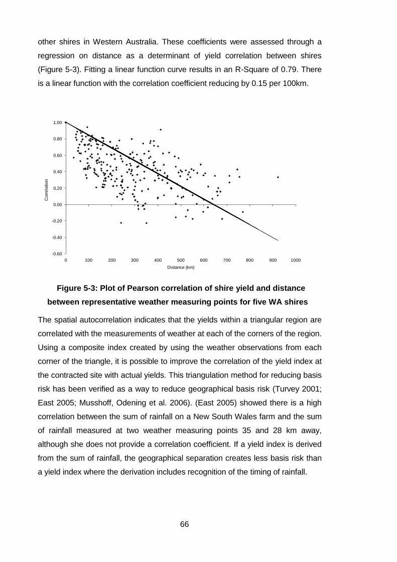
66

other shires in Western Australia. These coefficients were assessed through a

regression on distance as a determinant of yield correlation between shires

(Figure 5-3). Fitting a linear function curve results in an R-Square of 0.79. There

is a linear function with the correlation coefficient reducing by 0.15 per 100km.

Figure 5-3: Plot of Pearson correlation of shire yield and distance

between representative weather measuring points for five WA shires

The spatial autocorrelation indicates that the yields within a triangular region are

correlated with the measurements of weather at each of the corners of the region.

Using a composite index created by using the weather observations from each

corner of the triangle, it is possible to improve the correlation of the yield index at

the contracted site with actual yields. This triangulation method for reducing basis

risk has been verified as a way to reduce geographical basis risk (Turvey 2001;

East 2005; Musshoff, Odening et al. 2006). (East 2005) showed there is a high

correlation between the sum of rainfall on a New South Wales farm and the sum

of rainfall measured at two weather measuring points 35 and 28 km away,

although she does not provide a correlation coefficient. If a yield index is derived

from the sum of rainfall, the geographical separation creates less basis risk than

a yield index where the derivation includes recognition of the timing of rainfall.

-0.60

-0.40

-0.20

0.00

0.20

0.40

0.60

0.80

1.00

0 100 200 300 400 500 600 700 800 900 1000

Distance (km)

Co

rre

latio

n .

67

5.5 Weather and yield data

The data used for this thesis is the daily rainfall data from the Bureau of

Meteorology for the following years: Corrigin (Station id: 10536)(1910-2004),

Kojonup (Station id: 10582)(1907-2003), Moora (Station id: 8091) (1907-2004),

Mullewa (Station id: 8095) (1907-2004), Ravensthorpe (Station id: 10633) (1907-

2004).

The wheat yield data used in this thesis is a set of shire level yield data detrended

to approximate the yield of each year given the technology available in 2004. The

data is for the period between 1929 and 2004 and has been supplied by the

Department of Agriculture and Food Western Australia.

5.6 Summary

This chapter has presented alternate means to derive a yield index and the

benefits of using each in creating a yield index contract. This discussion led into

the construction of the yield index contract and then the design of the market

around the contract.

The conclusion of the chapter is that there is significant benefit in using a yield

index construction rather than a weather index construction as the basis of a

product to hedge production risk. In designing the market, there needs to be

consideration of how the market ensures adequate liquidity to allow for minimal

disruption to trading in the market, and limiting transaction risk.

68

69

6 RAINFALL, YIELD AND PRICE MODELLING

In this chapter a Monte Carlo simulation is used to model the interaction of a

farmer with the derivative market. To enable the Monte Carlo simulation this

chapter presents the method to simulate rainfall that is subsequently used to

determine distributions for yield and contract prices.

6.1 Rainfall modelling

Rainfall simulation is in two stages. The first stage simulates the rain event where

there are two states, rain and no rain. The second simulates the quantity of

rainfall if the rain event is in the rain state and samples from a distribution of

historical rainfall. The model uses data from the Bureau of Meteorology (2008) for

weather stations in five representative shires of Corrigin, Kojonup, Moora

Mullewa and Ravensthorpe (see Section 5.4).

The probability of rain on a given day, changes depending on the rainfall state in

the proceeding two days (Srikanthan and McMahon 1985; Musshoff, Odening et

al. 2006). To model this clustering we have constructed a probability space where

the probability of rain is reliant on the rainfall history of the previous two days. The

reason for using two days in the rainfall history is due to the structure of the

dominant weather patterns in the wheatbelt. The weather patterns in winter are

driven by dominant frontal patterns, where fronts are likely to deliver measureable

rainfall over a period of one to two days. Given these rainfall patterns there is a

difference in the probabilities of rain and the observation of rain in days 2 and

three of a weather system. The probabilities for these transitions are calculated

through the actual data, using strings of rainfall events in weekly kernels to

generate sufficient confidence for the probabilities.

The method used in this section is based on the method used by Srikanthon and

McMahon (1985), where a sampling from a distribution based on historical

observations generates the simulated seasons. Srikanthon and McMahon (1985)

70

use a Box- Jenkins model to simulate data where the observations are based on

an autoregressive moving average. The transition matrices are determined

through historical events while the rainfall quantity is determined in one process,

sampling from a distribution of rainfall that is constructed from five sets. The

elements of the first four sets display a linear relationship, while the fifth set is an

exponential function (Srikanthan and McMahon 1985). An advantage of this

approach to is that distorted probabilities due to a low frequency of observations

for transitions between states as the observation of rainfall days is sparse

(Srikanthan and McMahon 1985). In the method used in this thesis, the sequence

of rainfall events is determined through a separate process to the actual rainfall

measurement.

For this thesis, R is an n×m matrix of rainfall events for a shire, where n is the

number of days in a year (n = 365) and m is the number of years of annual

observations for each shire. The data is limited to 365 days as the additional day

in leap years would have little impact on any modelling approach.

A set of matrices are created with the same dimensions as R that could be used

to derive a transition matrix. The initial step was to evaluate the presence of

rainfall on a given day. This step creates a matrix RA as a binary matrix where

01

00

,

,

,

ji

jiA

jiRif

RifR (6.1)

The second step creates a matrix RB of values to show the observations of rainfall

on the days immediately prior to the day of the year i, and the year j.

1,1,2

0,1,1

0,0,0

,2,1

,2,1

,2,1

,

A

ji

A

ji

A

ji

A

ji

A

ji

A

ji

B

ji

RRif

RRif

RRif

R (6.2)

The values in RC combine the data R

A and RB from the matrices to provide 6

mutually exclusive states for any one day that capture whether there was a rain

event on the day, and the rain state on the previous two days (6.3).

71

2,1,5

1,1,4

0,1,3

2,0,2

1,0,1

0,0,0

,,

,,

,,

,,

,,

,,

,

B

ji

A

ji

B

ji

A

ji

B

ji

A

ji

B

ji

A

ji

B

ji

A

ji

B

ji

A

ji

C

ji

RRif

RRif

RRif

RRif

RRif

RRif

R (6.3)

A transition matrix for each week is then derived from RC. To increase the number

of observations the model can use to generate rainfall state probabilities, the

transition matrices are created using data for the given week from all available

years of data and the two adjacent weeks of the year.

The result is a transition matrix with the probability of making the transition from

the current rainfall state to another. One transition matrix is generated for each

week. Using a random number simulator, the model then uses the transition

matrices to simulate a sequence of rain and non-rain days for each week of a

season.

6.1.1 Rainfall density

The method used to simulate rainfall depth is a sampling from an expected

distribution of rainfall.

For this purpose we constructed a set of distributions based on weekly rainfall.

We use historical data to determine the distribution of rainfall depth for each of

the 6 potential states for each week. Matrix CR is used to filter the actual rainfall

events and compile a set of observations for each rainfall state. We then use

these observations to create three state dependant distributions of rainfall depth

for each week of the year. The rainfall depth is then sampled from this distribution

when the state simulation model declares a rainfall event.

72

Table 6-1: Comparison of means (µ) and variance (σ) of observed

and simulated rainfall

Observed GSR Modelled GSR

Mean Standard

deviation

Mean Standard

deviation

Corrigin 241.7 56.9 222.5 43.6

Kojonup 361.4 80.3 354 57.9

Moora 330.8 79.8 319.7 57.2

Mullewa 232.7 68.5 230.7 70.8

Ravensthorpe 218.3 59.3 216.5 61.5

In Table 6-1 there is some discrepancy between the simulated results and the

observed historical values. This discrepancy is greater in the annual rainfall (not

in table) where the modelled results do not adequately reflect the summer storm

events during January and February.

6.2 Yield modelling

This section describes the how the yield outcomes for each season are

generated. The yield outcomes are a function of the simulated rainfall.

The historical yield data used for the calibration test is the simulation of yield

using the Stress Index Model (STIN) as (see (Stephens, Lyons et al. 1989)). By

using historical seasonal data and the current yield efficiencies, the impact of

technology is not expressed. However, as the data is compiled as an indicative

shire yield using rainfall data from a range of weather stations across the shires,

the variance in the data is less than on farm observations of yield.. This effect

shown in Popp et al. (2005) where aggregate variance in spatially aggregated

crop yield could be half of the actual on farm variance. For this reason the yield

73

model returns the same mean yields as the raw data, though the variance is

higher. This result is consistent with Popp et al. (2005).

When the historical yield data had been normalised, the data were subject to the

Kolmogorov Smirnov test for normality of distribution with significance at 5%, the

hypothesis that the observations were a normal distribution was rejected. This

result is consistent with other studies (Just and Weninger 1999; Atwood, Shaik et

al. 2003). Nelson and Preckel characterises the yield distribution as a conditional

beta distribution (Nelson and Preckel 1989) although Martin and Barnett (2001)

show that the probable distribution of rainfall follows a gamma distribution. The

result with the historical data is counter to the findings in other studies (Just and

Weninger 1999; Atwood, Shaik et al. 2003) who suggest there may be non-

empirical reasons for misspecification of yield distributions such as the inclusion

of non-random elements. The argument that yield distribution is distorted into

non-normal distributions through non-random elements means finding the real

distribution is not feasible, and normality of yield distribution is preferable option.

However, the yield data used in this study has been generated through a yield

model, and thus only displays the effect of the weather data on yield, and not the

farmer's management. On using the Jaque-Brera and Kolmogorov-Smirnov tests,

normality of the simulated yield distribution is rejected when tested at a 5%

significance level.

This thesis uses the French and Schultz (1984) model determine the expected

yield (see section 5.1.2). French and Schultz (1984) is modified to incorporate

expected rainfall to provide an expected yield as the season progresses.

French and Schultz (1984) used the following function for expected yield at time

T:

)( bRaY TT (6.4)

The modification to the model is to incorporate a variable water loss function set

at 30% of seasonal rainfall, and to incorporate the observed and expected

components of the rainfall. These changes to the water loss function have been

recommended through personal communications (Bowran 2011). Thus the

(French and Schultz 1984) is modified to the following:

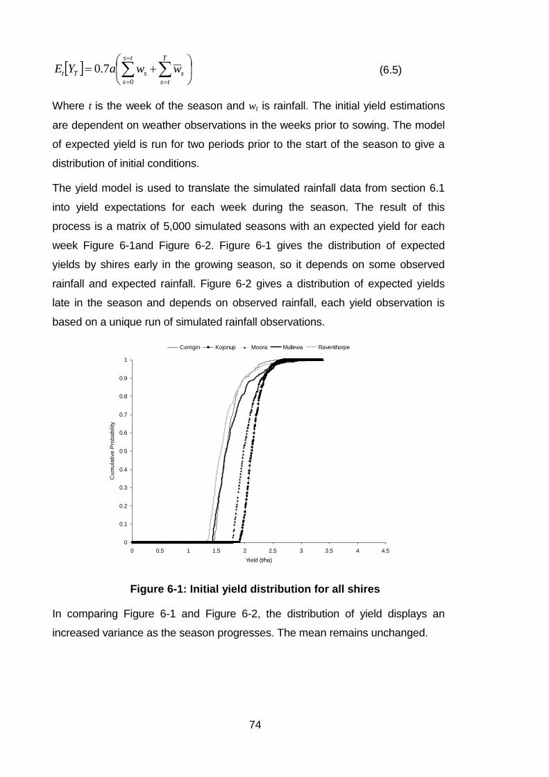
74

T

ts

s

ts

s

sTt wwaYE0

7.0 (6.5)

Where t is the week of the season and wt is rainfall. The initial yield estimations

are dependent on weather observations in the weeks prior to sowing. The model

of expected yield is run for two periods prior to the start of the season to give a

distribution of initial conditions.

The yield model is used to translate the simulated rainfall data from section 6.1

into yield expectations for each week during the season. The result of this

process is a matrix of 5,000 simulated seasons with an expected yield for each

week Figure 6-1and Figure 6-2. Figure 6-1 gives the distribution of expected

yields by shires early in the growing season, so it depends on some observed

rainfall and expected rainfall. Figure 6-2 gives a distribution of expected yields

late in the season and depends on observed rainfall, each yield observation is

based on a unique run of simulated rainfall observations.

Figure 6-1: Initial yield distribution for all shires

In comparing Figure 6-1 and Figure 6-2, the distribution of yield displays an

increased variance as the season progresses. The mean remains unchanged.

0

0.1

0.2

0.3

0.4

0.5

0.6

0.7

0.8

0.9

1

0 0.5 1 1.5 2 2.5 3 3.5 4 4.5

Yield (t/ha)

Cu

mu

lative

Pro

ba

bility .

Corrigin Kojonup Moora Mullewa Raventhorpe

75

Figure 6-2: Final yield distributions for all shires

The yield output of the model has been normalised by dividing the result by the

mean yield to so that the output of the model is the expected yield as a ratio of

the mean yield to generate the yield index Qm as in (6.6).

Y

YEQ Ttm (6.6)

This is an important distinction, and means the yield index contract does not

insure a grain yield, i.e. a yield per hectare of crop, instead insuring against a

change from expected production. The reason for creating the contract in this

manner is that the yields of farmers are going to be different, even at a very

similar locale due to soil and local geographical effects on weather. As an

example of how this index works, if the expected yield for the season was the

long term average, the index would be the value 100 representing an expected

average year. If there were an expected 10% reduction in production the yield

index would be 90.

6.2.1 Deriving the yield distribution

For the farmer to estimate an expected utility from crop production, before and

during the season, the farmer must know the expected distribution of the crop

yield. We simulate the expected crop yield for a season based on the observed

0

0.1

0.2

0.3

0.4

0.5

0.6

0.7

0.8

0.9

1

0 0.5 1 1.5 2 2.5 3 3.5 4 4.5

Yield (t/ha)

Cu

mu

lative

Pro

ba

bility .

Corrigin Kojonup Moora Mullewa Raventhorpe

76

values of rainfall up to t and the expected rainfall for t→T. The method used to

determine the expected distribution uses the set of yield outcomes from the

simulated seasons.

The model selects the seasons that have similar observed rainfall from the set of

simulated seasons. For any time prior to the end of the season, there is a set of

20,000 expected yields. To select the similar seasons, we firstly sorts the

seasons in increasing order of index value. We then select the 250 seasons

where the index at the given time is greater than the current season, though by

the smallest amount. The model then selects the 250 seasons where the index at

the given time is less than the current season, though by the smallest amount.

These outcomes in the final period of the selected seasons provide an

approximation of the expected yield distribution.

The index value at the given time is the expected yield. The distribution of

expected yield is used to determine the variance of the profit and the price of the

derivative contract that is presented in the following section.

6.3 Pricing the yield index contracts

6.3.1 Uncertainty in yield distributions

There has been disagreement over the shape of yield distributions and the effect

that data aggregation has on economic modelling (Debrah and Hall 1989; Just

and Weninger 1999; Ker and Goodwin 2000; Atwood, Shaik et al. 2003; Popp,

Rudstrom et al. 2005). There has generally been an implicit assumption that the

distribution of yields is a normal distribution, however, this is not always the case

in analysis of historical yield data. In Atwood et al. (2003) a re-examination of the

assumption of normality in yield distribution rejects the hypothesis of yield

normality. This result also occurs in Just and Weninger (1999) where it is stated

that historical methodological problems have led to false recommendation of crop

yield normality. Added to the uncertainty in yield distribution is the effect of

aggregation of data on yield variance that has been shown to display much

higher values when disaggregated to the farm level (Debrah and Hall 1989;

Popp, Rudstrom et al. 2005).

77

6.3.2 Derivation of the contract price

For this thesis we use the burn analysis for pricing the contracts as a robust

model suggested by Alaton (2002) that takes into account the uncertainty in yield

distribution. This method as used in Turvey et al. (2006) and Alaton bypasses the

problem of analytically estimating the change in distribution over time. Musshoff

et al. (2006) use the mean of discounted payoff rates for a rainfall index, based

on 56 historical observations. Jewson and Brix (2005) state that burn analysis is

a simple way to determine option pricing, that involves the calculation of historical

payoffs of an option, then finding the mean of the historical payoff. This thesis

uses the data generated by the yield model to complete the burn analysis. The

price of the contract for each week is the mean discounted value of the contract

at maturity plus a variable transaction cost. The methodology in section 6.3.1

generates a distribution of expected yield for each week during the season.

The farmer pays the transaction costs when participating in the market. There are

two components of transaction costs. The first is a fixed cost, which occurs due to

the construction of the market and the role of the broker in the market. The fixed

cost is borne by the farmer when they buy the contracts on the market. The

variable transaction costs are determined as a percentage of the contract value

and include the market price of risk.

The variable transaction costs are the sum of the liquidity risk and the timing risk

(6.7). ,

tm (6.7)

where the total transaction cost is λ,composed of the market rate for risk λm and

the cost of the timing risk λm.

The cost of the timing risk is an additional percentage of the current contract

price, equal to the expected cost of an adverse shift in contract price between

entering the market and settling the trade as in (6.8). The cost is not a fixed

percentage as is it based on an estimate of a change in price before settling

trades.

nntttC

entCtCE

h

hh

rn

t

(6.8)

78

Where tC h is the contract price at time t , n is the period of time between an

order being place in the market and the settling of the order. The hedge ratio at

time t and t + n is given by t and nt respectively. The sign of t depends

on whether the order in the market is a purchase or sell order. The transaction

cost is a fee that the trader requires as an incentive to enter the market given the

riskiness of the contract. The farmers view the cost as a transaction cost that is

excess to the actuarial premium.

6.4 Summary

This chapter shows how the rainfall is simulated, and how the simulated rainfall is

used to derive an expected yield. The expected yield for each simulated season

is then used to complete a simulated burn analysis to provide an option price for

every state (yield) and time during the season.

This state by time data is then accessible to the model of farmer decision making

to determine when the farmer will choose to change the hedge ratio, given risk

aversion and a myopic outlook. This model of farmer decision making is analysed

in chapter 8.

79

7 FARMER DECISION MAKING

This chapter defines how this thesis models the farmer's decision-making

process. It incorporates elements of the theory chapter into the applied model.

The chapter has three sections. The first section builds the utility function of the

farmer, starting with a static model of payoff, then introduces the capacity to

hedge production. Section 2 defines how farmers change their hedging strategy

based on rainfall during the season. The section derives the hedge ratio and

includes the timing of the farmer's decision to alter the hedged position. Section 3

describes how the model operates.

7.1 The model of expected utility

This section presents the model of farmer utility used in this thesis. The section

builds the utility model on a static payoff function. The static payoff function is

then extended into a time varying expected payoff function by introducing an

error term on the payoff. The static and expected payoff functions are then

combined into a model of expected utility.

7.1.1 Static payoff function

The simulation model focus solely on the hedging behaviour per unit of expected

production. While in Edwards and Simmons (2004) decisions regarding the area

planted and the hedge ratio need to be solved simultaneously, in this thesis, the

simultaneity problem does not exist. The thesis is looking at the hedging

behaviour during the season after the area has been planted.

We assume that there is only one crop type and a yield index contract is only

offered on this crop. This is reasonable in Western Australia where grain

production is dominated by wheat, (see Chapter 4 for details). We also assume

that there are no premiums or discounts for quality, consistent with Hertzler

(Hertzler 1999), and that there is no correlation between production and price

80

(Hertzler 1999; Edwards and Simmons 2004) (Simmons and Rambaldi 1997). In

other words WA with 3% of the world grain market is a price taker.

Specifically the value of the yield index contract at the start of the season is a

fixed quantity of grain Q~

where

1~

0

T

t

tqEQ (7.1)

And tq is a share of this quantity of grain that a farmer could sell in a forward

contract at time t. The term Q~

is an arbitrary quantity and set at one tonne of

grain for this thesis. The revenue for the expected unit of production is a function

of price and quantity

T

t

rt

tt eqpPQ0

(7.2)

tp is the price of forward price of grain at time t in $/tonne, r is a discount rate.

The total payoff function is defined as follows.

CPQYT (7.3)

Where is profit and Y is the total quantity of Q~

units of grain that the farmer

expects to produce, and C is the cost per unit of production of Q~

including

variable costs and fixed costs. Constructing the payoff function in this manner

removes area as a variable, and reduces the costs and prices to a value based

on a unit of production.

The costs of production for the season are known, and discounted to the initial

value by the discount rate. Given that the accrual of costs during the season

equates with the exercise of management options, the assumption of cost

certainty avoids additional complexity in modelling the impact of agronomic

management decisions during the season and the effects on yield distributions

and risk.

As an example, the quantity of production specified by the contract (Q~

) is 1

tonne. Where 1000Y , the farmer expects to produce 1000 tonnes of wheat per

year ( QY~

), for a cost of $170 per tonne (C ). The farmer can sell any portion of

81

the expected wheat production in any period for a forward price (tp ). If the spot

price is kept constant at $200/t then π = 1000×(200×(1)-170)=30,000.

To introduce a hedge into the profit function we use the yield index contract as

specified in section 5.2. The market is offering a contract with the strike (d) fixed

as a percentage of Q~

. If the modelled production is below the strike at T the

contract pays the farmer an indemnity. The farmers cannot exercise the contract

prior to maturity, though can sell the contract back to the market. Using an

adaptation of the notation from Section 2.2, the payoff of the contract at time of

maturity T is;

1,0max dPV TT (7.4)

The payoff of the contract is analogous to the payoff of a put option at time T. μ is

an error term equal to

Q

Qm

~1 (7.5)

Where mQ is the modelled production using observed and expected weather

conditions and is the yield index used as the underlying for the derivative. In this

case μ measures the modelled yield relative to expected. For instance, if Q~

is 1

tonne of wheat and the expected production Qm is 0.7 of the average, then µ is

the expected reduction in yield from the average, being 0.3, meaning that 30% of

expected production is foregone due to rainfall effects.

While there would be a difference between the modelled production and the

farmer’s production, that the thesis assumes that the farmer’s yield is exactly the

modelled yield. This eliminates the need for subscripts on the error term. This

assumption removes the geographical and local basis risk.

The payoff function at time T is altered from (7.3) and becomes

CVCPQY 11 (7.6)

Where is the number of contracts held by the farmer, and is the non actuarial

component of the contract premium. The cost of the hedged position is;

rtT

t

ttt eC

1

1 (7.7)

82

is the contract premium. A hedge ratio α is the number of contracts held to the

number of units of expected grain production given as

Y

(7.8)

Where 10 as there is an assumption that farmers do not speculate or take a

short position in the market. Dividing (7.6) by Y to derive profit per tonne

CVCPQT 11 (7.9)

as the payoff function at time T.

7.1.2 Expected payoff function

The introduction of multiple time periods changes the expected payoff function to;

ttt EE |1 (7.10)

Where t is the expected return per tonne at time T. The error term t is the

change in expected payoff for the period. The distribution is non-normal as in

Section 6.2.1 and the skew parameter of the distribution is an undefined function

of 1t . It has no upper bound and a lower bound of E .

The payoff function in (7.10) gives the farmers expectation of income at time T

while at time t<T. At time T, the payoff becomes known and reverts to the static

description as in (7.9). The thesis includes other simplifying assumption, that the

farmer can fix the price of grain at the start of the season.

Despite the non-normal distributions, the change in expected profit with respect

to time is zero. This characteristic of zero drift over time means that the index is

an unbiased estimator of the contract payoff at maturity.

7.1.3 Definition of the utility function

This paper uses a utility function with constant absolute risk aversion (CARA).

This is a preferred model of utility for use in a portfolio type analysis and is a

mean-variance model as in Newbury and Stiglitz (Newbery and Stiglitz 1981).

The assumption of CARA allows a range of functional forms including the form,

83

2

2 EE

kEUE (7.11)

Where k is the CARA coefficient of risk aversion. This model of utility is a

preferred form as it allows for negative payoffs (Peterson, Hertzler et al. 2000).

For the distribution of returns for farming in Western Australia, this is a preferred

characteristic.

To generate the coefficients of risk aversion the thesis used the methodology

from (Simmons and Rambaldi 1997). Bond and Wonder (1980) completed a

survey of Australian farmers to generate absolute risk aversion coefficients based

on a CARA utility function. Theses estimate, however, were based on a particular

distribution of initial wealth that does not apply to the farm population in WA.

While Bond and Wonder use the ELSE technique to determine the coefficients of

risk aversion, this method has received criticism (Anderson, Dillon et al. 1977;

Drynan 1981) based on the Equally Likely Certainty Equivalents (ELSE)

technique used to elicit the risk aversion coefficients. The criticism suggests that

the elicitation techniques could distort the estimation of the coefficient through not

eliminating several potential sources of bias, including the bias towards preferring

to gamble. While the critique is valid, they are the best estimates of risk aversion

coefficients for Australian farmers and have been widely utilised. Therefore to use

Bond and Wonder estimates in this study we use the following two step process

as used in Simmons and Rambaldi (1997):

Step 1: Convert from CARA coefficients to CRRA coefficients.

Step 2: Convert from CRRA back to CARA with wealth adjusted to appropriate

levels for this application.

The payoff function (7.9) and the expected payoff function (7.10) are then

substituted into the utility function (7.11) and the utility function becomes

211

2

11

tttt

ttt

VPQEVPQEk

CVCPQEUE

(7.12)

The control variable in this function is where it is the hedge ratio and can be

set by the farmer t a value between 0 and 1 inclusive. This maintains consistency

84

with the assumption that farmers do not speculate or assume a short position

with the contract. Taking the first derivative of (7.12) with respect to gives the

change in utility attributable to a change in the hedge ratio.

gEVgVkV

UEttt

t

2 (7.13)

The certainty equivalent derived from (7.12) becomes

CVCPQE tt 11 (7.14)

and the risk premium component of the utility function becomes

211

2tttt VPQEVPQE

k (7.15)

These functions are referred to in the results chapter.

7.2 Derivation of the hedge ratio

Chapter 2 showed the approaches used in the literature to determine the optimal

hedge in a portfolio. This section outlines the approach used in this thesis to

model the farmer’s hedging decisions.

7.2.1 Myopic decision maker

The farmer makes decisions based on the assumption that the decisions are not

revised before time T. If the initial decision is unaffected by the anticipation of

future revision, the optimal decision rule is said to be myopic (Karp 1987). A

myopic decision framework transforms a dynamic problem into a one period

discrete time problem (Karp 1988). The myopic model can only be applied when

the current price of the asset is an unbiased predictor of the future price of the

asset at every point in time. The solution for the hedge ratio in the myopic

scenario is given by Bray (1981). The solution can be solved in a static setting,

however the application is in asset markets where there is instantaneous

realisation of value from change in the underlying asset price. The model needs

to be altered for agriculture where change in the underlying, namely the weather,

does not necessarily create a shift in the expected income from production.

85

Here the farmer is assumed to be myopic. He makes a decision regarding the

optimal hedge at time t . The price of the derivative contract is an unbiased

estimator of the final price of the contract, and the decision made at this time is

the utility maximising hedge ratio given the expected distribution of profit at this

time. Given that the price of the contract is updated irrespective of farmer

expectations of the season, it changes as ntt . The farmer updates their

estimation of the seasonal outcomes at the same frequency that the yield index is

updated. To put this concept into a formal framework,

tfUE nttt ,,,, (7.16)

Where is a vector of potential outcomes for . The expectations regarding the

distribution of seasonal outcomes at nt are based on the information available

at t . The farmers decision to change the hedge ratio is made when there is

realisation that

tftf ntntt ,,,,,,

(7.17)

Where is the optimal hedge ratio at state μ. Where this condition holds, the

farmer no longer perceives the current hedge ratio as the optimal hedge ratio

given the expected seasonal conditions.

7.2.2 Switching mechanism

A farmer uses rainfall observation and the contract price to update their

perception of . Once the condition is satisfied, the farmer must make a decision

whether to change the hedge position and by what amount. Satisfying the

condition in does not mean that the farmer changes their hedge ratio. A farmer

does not adjust the hedge ratio, where this action incurs non-actuarial costs with

no utility benefit.

The farmer makes the decision to change the hedge ratio when the change in

utility from shifting to the optimal hedge ratio is greater than the transaction cost

of making the change

tntntt tftf

1,,,,,, (7.18)

Maturity approaches for the contract, and as μ approaches the strike mark d, the

distribution of optimal hedge ratio should follow a bimodal distribution. There are

86

two preferred hedge ratios at maturity of the contract depending on the value of μ

at T. These preferred hedge ratios are where the farmer is fully hedged where μ

is less than the strike d, and conversely the farmers' preferred hedge ratio is 0

where μ is greater than the strike d.

7.2.3 Dominance of hedging strategies

This thesis uses the certainty equivalent (7.11) to determine the preference of

one hedging strategy over another. While the farmer is maximising utility at all

points in time by altering their hedge ratios, it is possible that the result of using a

utility maximising hedging strategy does not improve the utility outcome of the

season. The farmer makes irreversible decisions during the season, and these

decisions while optimal at the time, may be suboptimal if the season were known.

The decision model used to determine the hedging decisions produces a certain

outcome in the final period. As the season progresses, the risk premium

component of the utility function reduces to zero as the variability in expected

return diminishes. This means that in the final time period, the return in any

season is equally preferred irrespective of the risk aversion of the farmer.

When the model is run over a number of seasons, the utility result of each

seasonal simulation is put into a column vector. It is possible to use the certainty

equivalent of the results vector, given the risk aversion coefficient used in the

model run, to determine value of a strategy that can be compared with other

strategies. The strategies can only be compared where the same risk aversion

coefficient is used.

7.3 The simulation methodology

Farmer’s participation in the yield index contracts market is assessed by Monte

Carlo simulation model. The simulated random variable is rainfall. The rainfall is

simulated for each of the 150 days of a growing season (Section 6.1). The daily

rainfall is then aggregated to create a total weekly observation of rainfall. Each

weekly sum of observed rainfall is used in the yield model to determine the effect

of the weeks weather on the expected yield. The result of the yield model is a

vector containing the expected production m

tQ for all 20 weeks of the growing

87

season. The production index in the final period m

TQ is the percentage of the

average yield that the farmer receives in the season. The expected production for

each week is used as the index on a market exchange.

The rainfall model simulates 20,000 growing seasons. These simulations are

maintained within a matrix. The yield index model is then used to create a matrix

of the same size to determine expected yield given the observed rainfall. The

price model calculates a contract price for every element in the yield model.

These three matrices are stored prior to running the model and accessed by the

simulation model.

When simulating a farmer’s decision making, the model randomly selects a row

vector from the yield and index matrix. A price vector is selected from the same

row in price matrix, as the rows in the price matrix are derived from the same row

in the yield matrix.

The farmer makes their optimal hedging decision for week one based on cell with

coordinates [1,1] in the yield and contract price vectors, and on the expected

distribution of yield in week one. The expected yield distribution is calculated

within the model as in Section .6.2.1

When the farmer has made the optimal hedging decision in week 1, the model

repeats the process for week two, based on the yield, price, and hedge ratio in

week 1, and deriving a new yield distribution for week 2. This process is repeated

for the 20 weeks in the season. When final week has elapsed, all variables are

reset, and the model selects another of the simulated seasons, and repeat the

process. The results in Chapter 8 are based on simulations of 1000 seasons.

7.4 Summary

This chapter has presented the model of farmer utility that is used in this thesis.

The simple model of farmer utility includes an option to hedge or change the

hedge ratio during the course of the season. The method used to determine

when the hedge is changed is shown within this chapter, including how and when

the farmer switches between the utility maximising hedge ratios, given their

myopic outlook.

88

This chapter finalised the model used in this thesis. The results from the model

are now presented in Chapter 8.

89

8 RESULTS

This chapter first determines whether spatial variability in production parameters

affect the demand for yield index contracts. Then it investigates whether alternate

methods of constructing a market affects demand for the derivative

8.1 Spatial differences in production and demand

This section analyses the initial demand for a yield index contract. For the

analysis, the simulation model for the farm decisions was run as in Chapter 7.

8.1.1 Initial hedging ratios

The expected wealth of the farmer at the start of each season is shown in Table

8-1. The initial expected incomes were compiled over four runs of 5,000

replicates of the model.

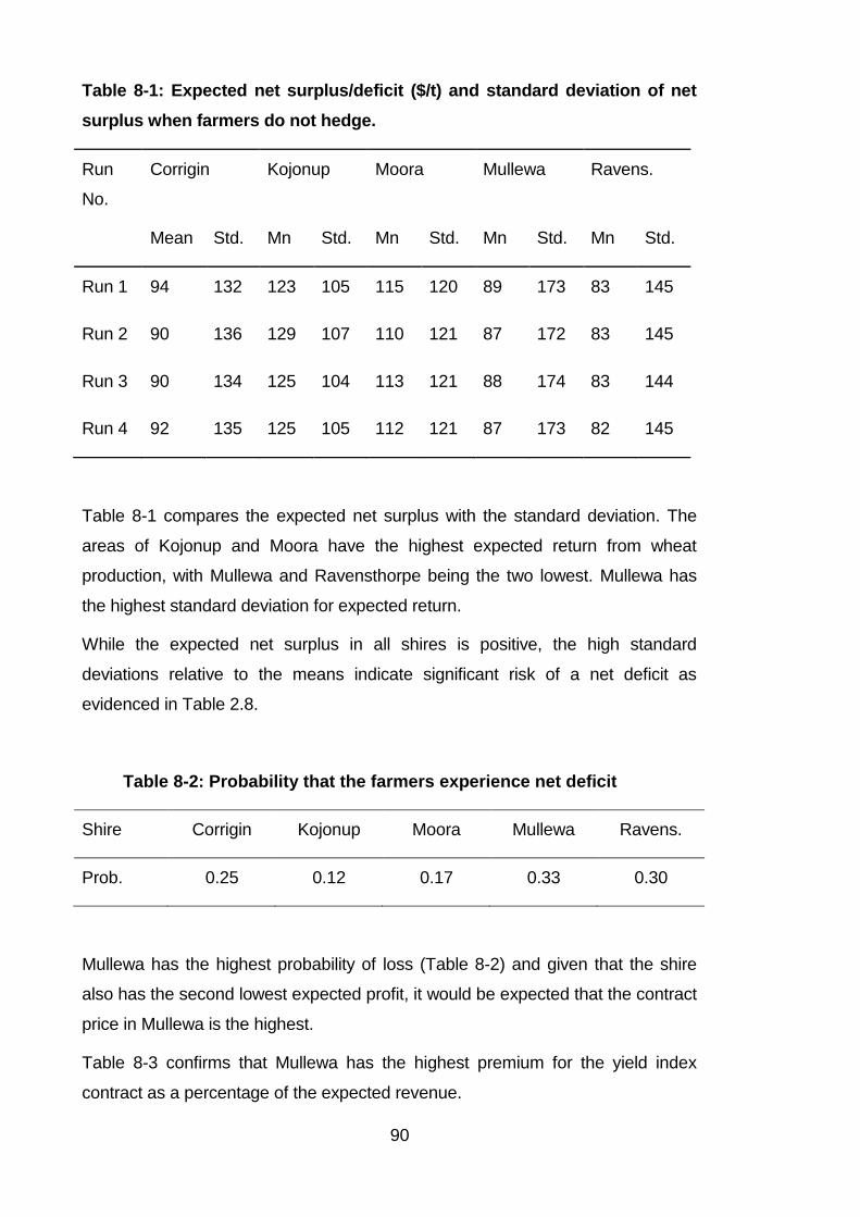
90

Table 8-1: Expected net surplus/deficit ($/t) and standard deviation of net

surplus when farmers do not hedge.

Run

No.

Corrigin Kojonup Moora Mullewa Ravens.

Mean Std. Mn Std. Mn Std. Mn Std. Mn Std.

Run 1 94 132 123 105 115 120 89 173 83 145

Run 2 90 136 129 107 110 121 87 172 83 145

Run 3 90 134 125 104 113 121 88 174 83 144

Run 4 92 135 125 105 112 121 87 173 82 145

Table 8-1 compares the expected net surplus with the standard deviation. The

areas of Kojonup and Moora have the highest expected return from wheat

production, with Mullewa and Ravensthorpe being the two lowest. Mullewa has

the highest standard deviation for expected return.

While the expected net surplus in all shires is positive, the high standard

deviations relative to the means indicate significant risk of a net deficit as

evidenced in Table 2.8.

Table 8-2: Probability that the farmers experience net deficit

Shire Corrigin Kojonup Moora Mullewa Ravens.

Prob. 0.25 0.12 0.17 0.33 0.30

Mullewa has the highest probability of loss (Table 8-2) and given that the shire

also has the second lowest expected profit, it would be expected that the contract

price in Mullewa is the highest.

Table 8-3 confirms that Mullewa has the highest premium for the yield index

contract as a percentage of the expected revenue.

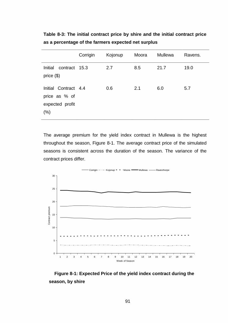
91

Table 8-3: The initial contract price by shire and the initial contract price

as a percentage of the farmers expected net surplus

Corrigin Kojonup Moora Mullewa Ravens.

Initial contract

price ($)

15.3 2.7 8.5 21.7 19.0

Initial Contract

price as % of

expected profit

(%)

4.4 0.6 2.1 6.0 5.7

The average premium for the yield index contract in Mullewa is the highest

throughout the season, Figure 8-1. The average contract price of the simulated

seasons is consistent across the duration of the season. The variance of the

contract prices differ.

Figure 8-1: Expected Price of the yield index contract during the

season, by shire

0

5

10

15

20

25

30

1 2 3 4 5 6 7 8 9 10 11 12 13 14 15 16 17 18 19 20

Week of Season

Contr

act

pre

miu

m

.

Corrigin Kojonup Moora Mullewa Ravesthorpe

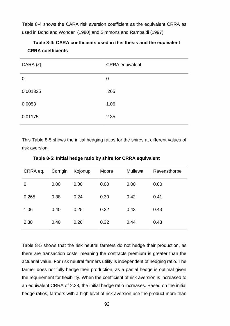
92

Table 8-4 shows the CARA risk aversion coefficient as the equivalent CRRA as

used in Bond and Wonder (1980) and Simmons and Rambaldi (1997)

Table 8-4: CARA coefficients used in this thesis and the equivalent

CRRA coefficients

CARA (k) CRRA equivalent

0 0

0.001325 .265

0.0053 1.06

0.01175 2.35

This Table 8-5 shows the initial hedging ratios for the shires at different values of

risk aversion.

Table 8-5: Initial hedge ratio by shire for CRRA equivalent

CRRA eq. Corrigin Kojonup Moora Mullewa Ravensthorpe

0 0.00 0.00 0.00 0.00 0.00

0.265 0.38 0.24 0.30 0.42 0.41

1.06 0.40 0.25 0.32 0.43 0.43

2.38 0.40 0.26 0.32 0.44 0.43

Table 8-5 shows that the risk neutral farmers do not hedge their production, as

there are transaction costs, meaning the contracts premium is greater than the

actuarial value. For risk neutral farmers utility is independent of hedging ratio. The

farmer does not fully hedge their production, as a partial hedge is optimal given

the requirement for flexibility. When the coefficient of risk aversion is increased to

an equivalent CRRA of 2.38, the initial hedge ratio increases. Based on the initial

hedge ratios, farmers with a high level of risk aversion use the product more than

93

those with a low level of risk aversion. The initial hedge ratios in the high risk

shires are higher than in the low risk shires.

This result is different to Edwards and Simmons (2004), where there is minimal

demand for weather derivatives by farmers with low coefficient of risk aversion. In

Edwards and Simmons (2004), the specification of the product is different, as

there is no real option available to the farmer to manage the portfolio.

8.1.2 Change in the distribution of hedge ratios over time

The hedge ratio decreases over time where a farmer is risk averse with a CRRA

coefficient greater than 0.265, in all shires except Kojonup (Figure 8.2). This

means that farmers purchases the optimal hedge in the initial period and sell the

hedge back to the market as the season progresses. The more risk averse

farmer is more likely to sell the contracts back to the market.

The mean hedge ratio diminishes as the season progresses for all shires at the

high levels of risk aversion. This occurs because there is a higher probability that

at the end of the season, the preferred hedging position would be a hedge ratio of

zero. This is due to the contract being out of the money more than in the money

at maturity. The standard deviation of the hedge ratio where the farmer has a

CRRA of 2.385 is higher than the standard deviation where the CRRA is 0.265.

The combination of the greater variance in hedge ratios and the diminishing

mean hedge ratio for the more risk averse farmer shows that they are more likely

to change their initial hedge ratio.

94

a)

b)

c)

d)

e)

f)

g)

h)

Corrigin Hedge Ratio | CRRA = 0.265

0.0

0.1

0.2

0.3

0.4

0.5

1 2 3 4 5 6 7 8 9 10 11 12 13 14 15 16 17 18 19 20

Week of Season

Mean H

edge R

atio

.

0.00

0.10

0.20

0.30

Std

Dev H

edge R

atio

.

Mean Std. Dev.

Corrigin Hedge Ratio | CRRA = 2.385

0.0

0.1

0.2

0.3

0.4

0.5

1 2 3 4 5 6 7 8 9 10 11 12 13 14 15 16 17 18 19 20

Week of Season

Mean H

edge R

atio

.

0.00

0.10

0.20

0.30

Std

Dev H

edge R

atio

.

Mean Std. Dev.

Kojonup Hedge Ratio | CRRA = 0.265

0.0

0.1

0.2

0.3

0.4

0.5

1 2 3 4 5 6 7 8 9 10 11 12 13 14 15 16 17 18 19 20

Week of Season

Mean H

edge R

atio

.

0.00

0.10

0.20

0.30

Std

Dev H

edge R

atio

.

Mean Std. Dev.

Kojonup Hedge Ratio | CRRA = 2.385

0.0

0.1

0.2

0.3

0.4

0.5

1 2 3 4 5 6 7 8 9 10 11 12 13 14 15 16 17 18 19 20

Week of Season

Mean H

edge R

atio

.

0.00

0.10

0.20

0.30

Std

Dev H

edge R

atio

.

Mean Std. Dev.

Moora Hedge Ratio | CRRA = 0.265

0.0

0.1

0.2

0.3

0.4

0.5

1 2 3 4 5 6 7 8 9 10 11 12 13 14 15 16 17 18 19 20

Week of Season

Mean H

edge R

atio

.

0.00

0.10

0.20

0.30

Std

Dev H

edge R

atio

.

Mean Std. Dev.

Moora Hedge Ratio | CRRA = 2.385

0.0

0.1

0.2

0.3

0.4

0.5

1 2 3 4 5 6 7 8 9 10 11 12 13 14 15 16 17 18 19 20

Week of Season

Mean H

edge R

atio

.

0.00

0.10

0.20

0.30

Std

Dev H

edge R

atio

.

Mean Std. Dev.

Mullewa Hedge Ratio | CRRA = 0.265

0.0

0.1

0.2

0.3

0.4

0.5

1 2 3 4 5 6 7 8 9 10 11 12 13 14 15 16 17 18 19 20

Week of Season

Mean H

edge R

atio

.

0.00

0.10

0.20

0.30

Std

Dev H

edge R

atio

.

Mean Std. Dev.

Mullewa Hedge Ratio | CRRA = 2.385

0.0

0.1

0.2

0.3

0.4

0.5

1 2 3 4 5 6 7 8 9 10 11 12 13 14 15 16 17 18 19 20

Week of Season

Mean H

edge R

atio

.

0.00

0.10

0.20

0.30

Std

Dev H

edge R

atio

.

Mean Std. Dev.

95

i)

j)

Figure 8-2: a-j. Mean and spread of shire hedge ratios for different

CRRA coefficients

Figure 8-3 displays the cumulative distribution function of the hedge ratios in

Mullewa when the farmer has a CRRA equivalent of 1.06. While there is a shift

from the initial hedge ratio with a flattening of the distribution curve, after week 15

the curve remains very similar. This shows that the farmer is unwilling to change

the hedge ratio in the later stage of the season. There are high contract prices

where the contract is in the money and little effect on the expected distributions of

return where the contract is out of the money.

.

Figure 8-3: Distribution of hedge ratios for Mullewa when CRRA is

1.32 for different weeks

At the start of the seasons (week 1) the mean hedge ratio is 0.47. As time

progresses (weeks 7, 14 and 20) the farms reduce or increase the hedge ratios.

Ravensthorpe Hedge Ratio | CRRA = 0.265

0.0

0.1

0.2

0.3

0.4

0.5

1 2 3 4 5 6 7 8 9 10 11 12 13 14 15 16 17 18 19 20

Week of Season

Mean H

edge R

atio

.

0.00

0.10

0.20

0.30

Std

Dev H

edge R

atio

.

Mean Std. Dev.

Ravensthorpe Hedge Ratio | CRRA = 2.385

0.0

0.1

0.2

0.3

0.4

0.5

1 2 3 4 5 6 7 8 9 10 11 12 13 14 15 16 17 18 19 20

Week of Season

Mean H

edge R

atio .

0.00

0.10

0.20

0.30

Std

Dev H

edge R

atio .

Mean Std. Dev.

0

0.2

0.4

0.6

0.8

1

1.2

0 0.2 0.4 0.6 0.8 1

Observed Hedge Ratio

Cum

ula

tive p

robabili

ty

.

Week 1 Week 7 Week 14 Week 20

96

It is expected that the farmer ends the season with a hedge ratio of 0 or 1. If the

farmer could choose the preferred hedge ratio in the final period the choice would

be 1 or 0, depending on whether the value of the index is below or above the

strike value respectively. This expected result does not occur in the data. The

distribution of hedge ratios does not collapse to a bimodal distribution. As time

approaches the final period, if the probability that the contract is valuable in the

final period approaches one, the optimal hedge ratio also approaches one.

However, the value from changing the hedge ratio approaches zero as the

expected profit from production becomes certain. Changing the hedge ratio does

not affect the variance of expected returns, hence the high cost of doing so is not

economic. As time approaches the final period, if the probability that the contract

is valuable in the final period approaches zero, the optimal hedge ratio also

approaches zero. In this scenario, the return on selling the contract back to the

market is less than the transaction cost, therefore no transaction is made.

8.1.3 The effect of spatial variability on demand

The production parameters of a region affect the farmers demand for the yield

index contract. In the high risk shires, the strategy of using the market dominates

the strategy of not using the market for higher levels of risk aversion (Figure 8-4).

In the shires of Moora and Kojonup the hedging strategy does not dominate the

non-hedging strategy at any level of risk aversion. In the shires of Ravensthorpe

and Corrigin, the hedging strategy dominates the non hedging strategy at the

highest tested level of risk aversion, while in the Mullewa shire the hedging

strategy dominates the non hedging strategy at the high and medium levels of

risk aversion.

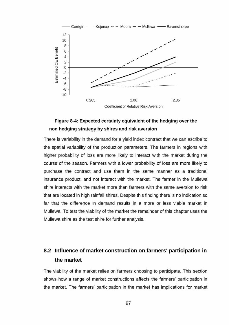
97

Figure 8-4: Expected certainty equivalent of the hedging over the

non hedging strategy by shires and risk aversion

There is variability in the demand for a yield index contract that we can ascribe to

the spatial variability of the production parameters. The farmers in regions with

higher probability of loss are more likely to interact with the market during the

course of the season. Farmers with a lower probability of loss are more likely to

purchase the contract and use them in the same manner as a traditional

insurance product, and not interact with the market. The farmer in the Mullewa

shire interacts with the market more than farmers with the same aversion to risk

that are located in high rainfall shires. Despite this finding there is no indication so

far that the difference in demand results in a more or less viable market in

Mullewa. To test the viability of the market the remainder of this chapter uses the

Mullewa shire as the test shire for further analysis.

8.2 Influence of market construction on farmers' participation in

the market

The viability of the market relies on farmers choosing to participate. This section

shows how a range of market constructions affects the farmers’ participation in

the market. The farmers’ participation in the market has implications for market

-10

-8

-6

-4

-2

0

2

4

6

8

10

12

0.265 1.06 2.35

Coefficient of Relative Risk Aversion

Estim

ate

d C

E B

en

efit .

Corrigin Kojonup Moora Mullewa Ravensthorpe

98

viability. The section gives results from the market in the Mullewa shire, as this

shire has the highest participation in the market during the season.

8.2.1 Dominance of the hedging strategy

There are two simple strategies where farmers have a choice to maximise utility

by using a contract to hedge production risk, either. The farmer uses the market

or does not use the market. Neither strategy dominates the other in the sense of

first degree stochastic dominance (Figure 8-5). In the sense of second degree

stochastic dominance, again neither strategy dominates the other (Figure 8-5).

This case occurs irrespective of the risk aversion of the farmer.

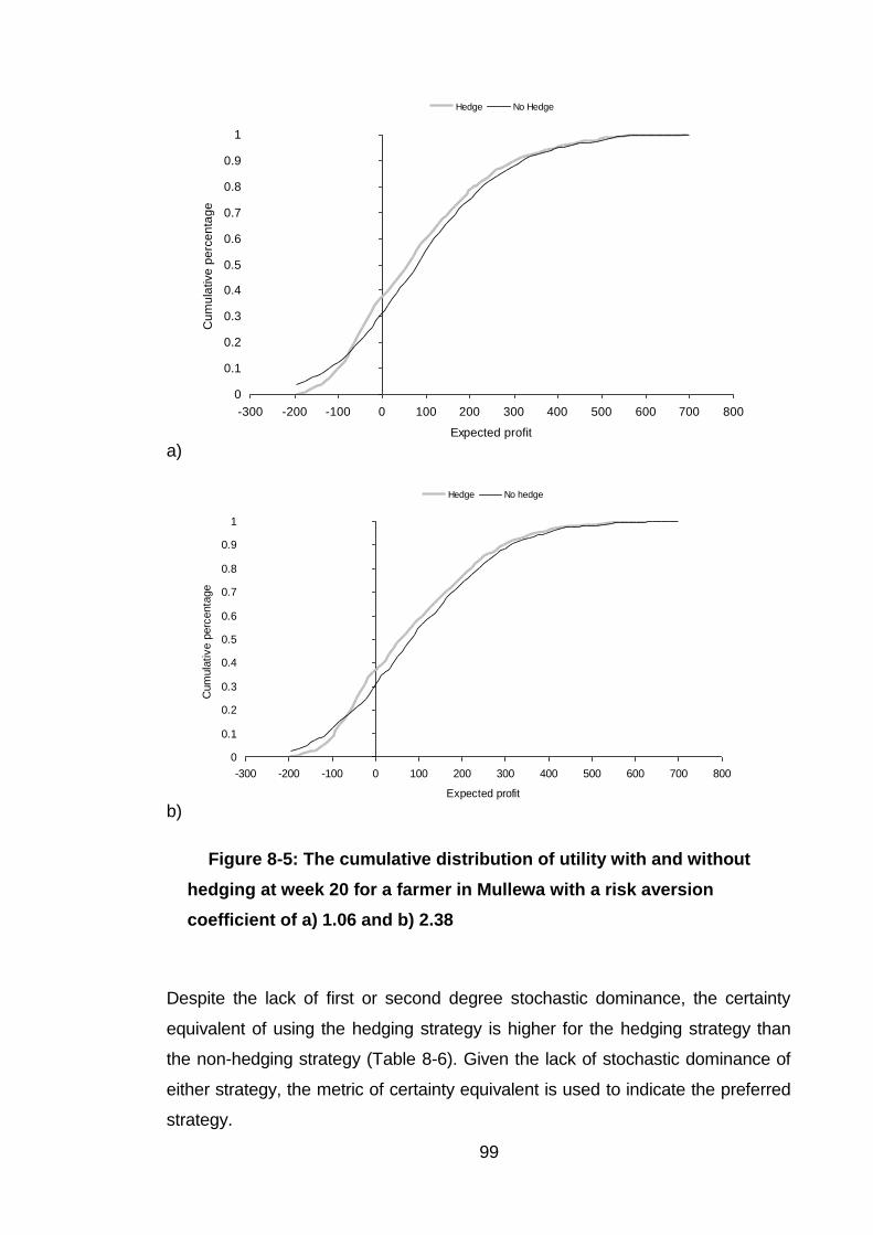
99

a)

b)

Figure 8-5: The cumulative distribution of utility with and without

hedging at week 20 for a farmer in Mullewa with a risk aversion

coefficient of a) 1.06 and b) 2.38

Despite the lack of first or second degree stochastic dominance, the certainty

equivalent of using the hedging strategy is higher for the hedging strategy than

the non-hedging strategy (Table 8-6). Given the lack of stochastic dominance of

either strategy, the metric of certainty equivalent is used to indicate the preferred

strategy.

0

0.1

0.2

0.3

0.4

0.5

0.6

0.7

0.8

0.9

1

-300 -200 -100 0 100 200 300 400 500 600 700 800

Expected profit

Cu

mu

lative

pe

rce

nta

ge

.

Hedge No Hedge

0

0.1

0.2

0.3

0.4

0.5

0.6

0.7

0.8

0.9

1

-300 -200 -100 0 100 200 300 400 500 600 700 800

Expected profit

Cum

ula

tive p

erc

enta

ge

.

Hedge No hedge

100

Table 8-6: Comparison of expected utility for hedging and non

hedging strategies for Mullewa with CRRA = 1.06

E(U)

Hedging strategy 7.34

Non-Hedging strategy 3.8

This is an important result though one predicted by theory. If the premium is

actuarially correct, the expected profit of each strategy is equivalent. Given that

the farmer in this thesis and specifically this section is risk averse, the farmer

prefers the strategy of choosing to hedge production risk to the strategy of not

hedging production risk.

8.2.2 Alternate market scenarios and the effect on farmer demand

This remainder of section 8.2 compares the hedging behaviour in 6 market

scenarios. This section determines the preferred market construction and the

market constructions are presented in Table 8-7. The scenarios in this section

are tested under the assumption of minimal transaction costs that include a fixed

cost of participation in the market and a proportional market price of risk

additional to the actuarial price. Each market scenario is a change in the

construction of the market.

101

Table 8-7: Detail on the alternative market constructions

Construction Week number of season when farmer can change hedge ratio

1. No hedging

2. All weeks

3. 1

4. 1 4 7 10 13 16 19

5. 1 3 8 13 18

6. 1 5 13 20

Comparing the expected utility from each market construction with the strategy of

not hedging, shows that farmers with different risk aversions would benefit from

different market constructions (Table 8-8). No singular construction is preferred

by all farmers.

Table 8-8: Difference in expected utility between using the given

market construction and a no hedging strategy

Construction CRRA coefficients of risk aversion

.265 1.06 2.35

2. -4.41 3.56 17.61

3. 1.83 9.08 21.81

4. -1.02 9.77 17.21

5. 0.01 10.28 23.81

6. 0.98 12.14 20.57

102

The farmers with a low aversion to risk prefer the insurance type market

(Construction 3). Their last preference is for the market where they can trade the

contracts continuously (Construction 2). These farmers prefer the strategy of not

hedging to using the continuously traded market, and the market where there are

seven opportunities to change hedge ratios (Construction 4). The farmers with a

moderate level of risk aversion prefer the market construction where there are

four opportunities (Construction 6) to change hedge ratios in the market. The

farmers with a high level of risk aversion are ambivalent between the market

construction with four or five options to change hedge ratios, and the insurance

type of market. In all cases, the market construction where a farmer can trade

continuously is the least preferred.

8.2.3 Relationship between the contract price, risk premium and supply

of the contract to the market

In this section, the relationship between the supply of the contract to the market

and the risk premium component of the utility function is presented (Figure 8-6).

When a contract is sold by the farmer, the farmers' hedge ratio decreases. When

the farmers' hedge ratio is decreased there is an increase in supply of the

contracts into the market. The supply curve for the contract is presented as the

quantity of contracts supplied to market (Figure 8-6a).

There is a switching point between buying and selling the contract in the market

in response to the price of the contract. There is a tendency for farmers to

increase supply of the contract to the market where there is a higher price for the

contract, and demand more of the contract when the price is lower. There is a

positive correlation between price and supply with coefficient of 0.0011.1 The

1 Regression function of form y = -0.104 + 0.0011x where supply is a responsive function of price.

Standard error R2 0.045 0.507

103

supply elasticity at the mean is 0.08. This occurs as the benefit of holding the

contract in reducing risk is declining as shown by the trend in the 'risk premium'

curve. The price where the farmer’s behaviour switches occurs when the value of

holding the contract in reducing variance is less than the utility value of selling the

hedge.

The curve showing the relationship between the value of holding the contract and

the contract premium (Figure 8-6a) has a negative slope until the contract

premium reaches approximately $60. At this price the contract is deep in the

money and the variance of the portfolio is stable, with respect to changes in the

contract price. At this point the farmer sells the contract back to the market and

accepts an increase in variance on crop returns for a certain return from the

contract sale.

The supply curve for Scenario 2 is no longer apparent (Figure 8-6b). The

relationship between price and supply has broken down2. Where the farmer does

change their hedge ratio, there is a low correlation between price and supply into

the contract market. Figure 8-6b does not show the effect that previous

interactions with the market have on the current quantity contracts held by

farmers. This effect is also due to the myopic decision making of the farmer,

where farmers do not respond to market signals in the contract market, though do

respond to perceived changes in expected yield. To determine whether there is a

supply response the effect of a risk premium on the yield contract is shown

Section 6.3.

2 Note that the farmer is not required to change the hedge ratio at this point in time due to the myopic nature

of the farmers decision making.

104

a)

b)

Figure 8-6: Relationship between contract premium and the risk

premium; and contract premium and the supply of the contract to the

market at week 15, for two scenarios. a) Scenario 2: Farmer can

change hedge at any time b) Scenario 5: Farmer can change hedge at

5 week intervals

8.3 Viability of the proposed yield index contract

This section presents the results on the viability of the market for these yield

index contracts. The results from Section 8.2 show the value to the farmer from

-0.4

-0.3

-0.2

-0.1

0

0.1

0.2

0.3

0.4

0.5

0 50 100 150 200

Price of Contract

Ch

an

ge

in

He

dg

e R

atio

.

-0.4

-0.3

-0.2

-0.1

0

0.1

0.2

0.3

0.4

0.5

0 50 100 150 200

Price of Contract

Ch

an

ge

in

He

dg

e R

atio

.

105

using the contracts. This section assesses if there is adequate liquidity to create a

viable market when there are transaction costs. The form the transaction cost is a

loading factor on the actuarial premium.

The loading factor is perceived by the farmer as an additional cost, though is

perceived by traders as the cost to counter the risk of an adverse shift in the

value of the asset.

To determine the equilibrium and provide an understanding of the change in

behaviour under fixed transaction cost, the model is run with a range of

transaction costs.

8.3.1 Effect of additional transaction risk on initial hedge ratio

As the transaction cost increase, farmers reduce their initial hedge ratios. This

imposes an immediate threshold on the transaction costs, above which a market

is not used by farmers. For representative farmers with a low level of risk

aversion, this immediate threshold is at 45% of the actuarial price. Figure 8-7

presents the relationship between the percentage of the premium that is incurred

as a transaction cost and the initial hedge ratio. Under all scenarios of risk

aversion, the initial hedge ratio declines with an increase in transaction costs.

106

Figure 8-7: Relationship between percentage increase of the non

actuarial premium and the initial hedge ratio for multiple coefficients

of risk aversion in the Mullewa Shire.

8.3.2 Affect of liquidity on transaction risk

An illiquid market causes transaction risk for speculators. Transaction risk is

costed through liquidity and volatility costs and are incorporated into the

speculators bid prices in the market (Section 6.3). Volatility costs occur when

there is a lag between the bid in the market and the acceptance of the bid, in

which time the price of the asset changes. As farmers do not interact with the

market on a continuous basis, volatility costs are incurred by the speculators.

8.3.3 Liquidity in the market

The level of liquidity affects the viability of the market. As we showed in Section

6.3 the value of offers as a percentage of the total value of the unclosed positions

in the market provides a measure of liquidity (Schwartz and Francioni 2004). The

key results for liquidity regard the behaviour of the farmers in the market. The

volume of trade as a percentage of the open positions declines during the course

of the season. This trend occurs irrespective of the level of transaction cost

(Figure 8-8).

0.00

0.05

0.10

0.15

0.20

0.25

0.30

0.35

0.40

0.45

0.50

0.05 0.10 0.15 0.20 0.25 0.30 0.35 0.40

Percentage

Iniita

l H

ed

ge

Ra

tio

.

CRRA = 0.265 CRRA = 1.06 CRRA = 2.35

107

Figure 8-8: Farmer offers in the market as a percentage of total

unclosed positions by initial fixed transaction cost

The decline in the liquidity in the market during the season occurs irrespective of

the transaction cost. The result is dependant on the measure of liquidity being the

quantity of offers in the market as the percentage of unclosed positions. There

are few transactions in the high transaction cost markets after the initial four

weeks (Figure 8-9). Where there is an additional transaction cost of 30% of the

actuarial premium, there is little interaction with the market after week 4.

0.00%

0.20%

0.40%

0.60%

0.80%

1.00%

1.20%

1.40%

1.60%

Week 1 Week 4 Week 7 Week 10 Week 13 Week 16 Week 19

Week of Season

% o

f M

ark

et

Valu

e

.

0.05 0.15 0.30 0.40

0

0.2

0.4

0.6

0.8

1

1.2

Week 1 Week 4 Week 7 Week 10 Week 13 Week 16 Week 19

Week of Season

% o

bse

rva

tio

ns: ch

an

ge

he

dg

e r

atio

o . 0.05 0.15 0.30 0.40

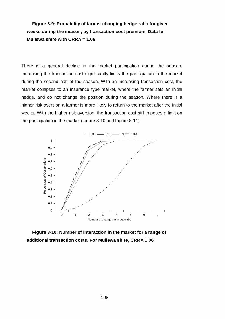
108

Figure 8-9: Probability of farmer changing hedge ratio for given

weeks during the season, by transaction cost premium. Data for

Mullewa shire with CRRA = 1.06

There is a general decline in the market participation during the season.

Increasing the transaction cost significantly limits the participation in the market

during the second half of the season. With an increasing transaction cost, the

market collapses to an insurance type market, where the farmer sets an initial

hedge, and do not change the position during the season. Where there is a

higher risk aversion a farmer is more likely to return to the market after the initial

weeks. With the higher risk aversion, the transaction cost still imposes a limit on

the participation in the market (Figure 8-10 and Figure 8-11).

Figure 8-10: Number of interaction in the market for a range of

additional transaction costs. For Mullewa shire, CRRA 1.06

0

0.1

0.2

0.3

0.4

0.5

0.6

0.7

0.8

0.9

1

0 1 2 3 4 5 6 7

Number of changes in hedge ratio

Pe

rce

nta

ge

of O

bse

rva

tio

ns .

0.05 0.15 0.3 0.4

109

Figure 8-11: Number of interaction in the market for a range of

additional transaction costs. For Mullewa shire, CRRA 2.35

8.3.4 Expected cost of transaction risk

The components of transaction risk change depending on the market structure.

As in Section 6.3, this thesis models transaction risk as the additional cost due to

liquidity and timing risk.

The required transaction risk premium on entering the market for the traders

increases over the course of the season. This reflects fewer opportunities for

closing the position as it is less likely that the farmers make significant changes to

their hedge ratio late in the season, given that farmers become increasingly

certain of their level of production. This limited farmer participation in the market

near the end of the season results in limited liquidity and depth.

The results show that the total premium loading required by speculators is higher

that the tested initial transaction cost loadings (Figure 8-12 and Figure 8-13). This

shows that the market is not in equilibrium where the transaction costs loadings

are in the tested range.

0

0.1

0.2

0.3

0.4

0.5

0.6

0.7

0.8

0.9

1

0 1 2 3 4 5 6 7

Number of changes in hedge ratio

Pe

rce

nta

ge

of O

bse

rva

tio

ns .

0.05 0.15 0.3 0.4

110

Figure 8-12: Non actuarial premium required by traders as a fee to

enter market due to transaction risk: market construction 4, Mullewa

Shire, Model run with no initial transaction risk premium

Figure 8-13: Non-actuarial premium required by traders as a fee to

enter market due to transaction risk: market construction 4, Mullewa

Shire, Model run with initial transaction risk premium of 30%

As the transaction cost in the market increases, the fee in the form of contract

price loadings that the traders require to enter the market, also increases. As the

transaction costs increase, the farmer's participation in the market is reduced.

The reduction in farmer's participation again increases the fee that traders require

to enter the market. The market is not in equilibrium, as the transaction cost

required by the market does not converge with the initial transaction cost

incorporated into the modelling, to stabilise demand through the season. The

effect of this increasing transaction cost through time is the contraction of the

-

0.20

0.40

0.60

0.80

1.00

1.20

1.40

Week 1 Week 4 Week 7 Week 10 Week 13 Week 16 Week 19

Week of Season

% o

f V

alu

e .

0.265 1.060 2.350

-

0.20

0.40

0.60

0.80

1.00

1.20

1.40

Week 1 Week 4 Week 7 Week 10 Week 13 Week 16 Week 19

Week of Season

% o

f V

alu

e .

0.265 1.060 2.350

111

farmer demand to the early part of the season where there is still high uncertainty

in production.

8.3.5 Effect of additional transaction risk on dominance of hedging

strategy

There is an upper threshold on the loading factor above which the hedging

strategy does not dominate the strategy of not hedging (Figure 8-14). For the

farmer with a moderate level of risk aversion (CRRA = 1.06), a loading above 0.4

results in not-hedging being the dominant strategy (Figure 8-15).

The dominance of the hedging strategy over the non-hedging strategy is minimal

for farmers, in both market constructions. When there is an increase in

transaction costs, the representative farmer does not realise utility benefit from

using a yield index contract.

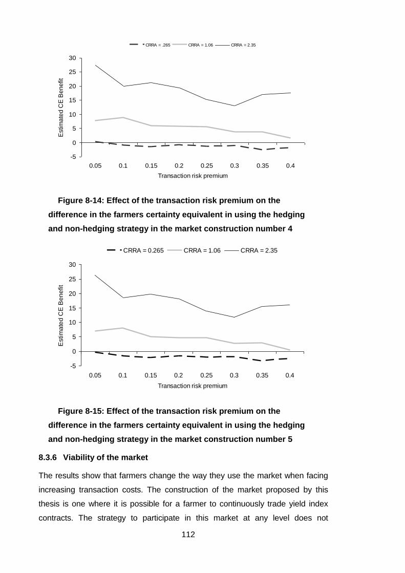
112

Figure 8-14: Effect of the transaction risk premium on the

difference in the farmers certainty equivalent in using the hedging

and non-hedging strategy in the market construction number 4

Figure 8-15: Effect of the transaction risk premium on the

difference in the farmers certainty equivalent in using the hedging

and non-hedging strategy in the market construction number 5

8.3.6 Viability of the market

The results show that farmers change the way they use the market when facing

increasing transaction costs. The construction of the market proposed by this

thesis is one where it is possible for a farmer to continuously trade yield index

contracts. The strategy to participate in this market at any level does not

-5

0

5

10

15

20

25

30

0.05 0.1 0.15 0.2 0.25 0.3 0.35 0.4

Transaction risk premium

Estim

ate

d C

E B

en

efit .

CRRA = .265 CRRA = 1.06 CRRA = 2.35

-5

0

5

10

15

20

25

30

0.05 0.1 0.15 0.2 0.25 0.3 0.35 0.4

Transaction risk premium

Estim

ate

d C

E B

en

efit .

CRRA = 0.265 CRRA = 1.06 CRRA = 2.35

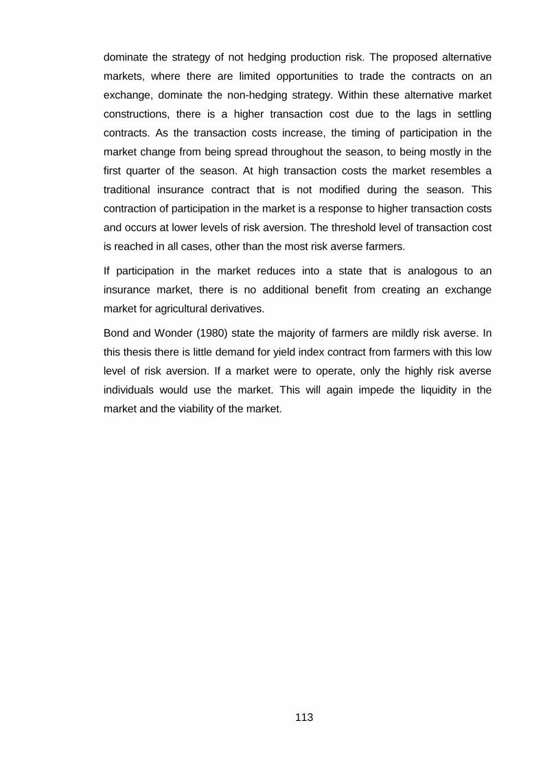
113

dominate the strategy of not hedging production risk. The proposed alternative

markets, where there are limited opportunities to trade the contracts on an

exchange, dominate the non-hedging strategy. Within these alternative market

constructions, there is a higher transaction cost due to the lags in settling

contracts. As the transaction costs increase, the timing of participation in the

market change from being spread throughout the season, to being mostly in the

first quarter of the season. At high transaction costs the market resembles a

traditional insurance contract that is not modified during the season. This

contraction of participation in the market is a response to higher transaction costs

and occurs at lower levels of risk aversion. The threshold level of transaction cost

is reached in all cases, other than the most risk averse farmers.

If participation in the market reduces into a state that is analogous to an

insurance market, there is no additional benefit from creating an exchange

market for agricultural derivatives.

Bond and Wonder (1980) state the majority of farmers are mildly risk averse. In

this thesis there is little demand for yield index contract from farmers with this low

level of risk aversion. If a market were to operate, only the highly risk averse

individuals would use the market. This will again impede the liquidity in the

market and the viability of the market.

115

9 CONCLUSIONS

This chapter discusses the three major conclusions from this thesis. The chapter

then makes recommendations for further research in the area following on the

findings in this thesis.

9.1 The effect of regional parameters upon demand

The thesis investigated the differences in the initial hedges in the different

regions. Two strategies were compared. The first strategy was for the farmers in

these shire to use the yield index contracts to hedge production risk with a

continuous trading strategy. The second strategy was to not use the yield index

contracts. For all farmers with a low level of risk aversion, the preferred strategy

is to not hedge production risk.

In the Mullewa shire, the preferred strategy for the moderate risk aversion was to

hedge production risk. For farmers with a high level of risk aversion, the hedging

strategy was preferred in Mullewa, Ravensthorpe and Corrigin shires.

Farmers in the low risk shires purchase a relatively small number of contracts.

Given that there is a high probability that the contract ends the season out of the

money, where there is no value to the farmer in exercising the contract, any up

front cost is lost. Farmers in the low risk shires, even with a high level of risk

aversion are not as willing to purchase a contract as in the high risk shires.

Analysis of the low risk shires was limited to this analysis of initial hedge ratios. In

low risk shires, wheat is a less dominant enterprise in the farming system. The

risk to whole farm profit from poor wheat production is less than in other regions.

116

9.2 The effect of market construction upon demand

An exchange market with weekly trading of index based agricultural derivatives in

Western Australia is not a preferred option for the provision of risk management

instruments.

Farmers with a high level of risk aversion prefer to use an exchange market for

trading yield index contracts over the option of not hedging production. However,

the market constructions with limited opportunities for trading are preferred over

the weekly trading construction. There is no benefit from the additional

opportunities to trade contracts. There is benefit in the markets with limited

opportunities to trade, above using the contract as a one off insurance,

purchased at the beginning of the year. Farmers regain some utility from selling

the contracts back to the market.

9.3 The viability of a market for yield index contracts

The viability of an exchange market for weather derivatives would be impaired by

a lack of liquidity and participation in the market. The additional premiums above

the actuarial premium would limit participation in the market. With a high

transaction cost premium, the farmer participation in the market collapses to a

state where the participation structure is the same as a traditional insurance

market. Farmers take an initial hedge and maintain the hedge ratio though the

season. At this point there is no benefit from creating a market exchange.

The major cause of non-viability in the market for agricultural derivatives is the

low liquidity in the market. There is some discussion that there would be

participation in the market from the secondary industry that relies on success of

agricultural production (Hertzler, Kingwell et al. 2006). This includes industry such

as the agricultural machinery industry. There is no guarantee that there is interest

from secondary industry to invest in the market and increase liquidity. A yield

index is only designed to be correlated to the yield of a particular crop, not the

revenue of a secondary industry. While there is a high correlation between crop

yields and machinery sales, the payoff on a near continuous index may not

provide adequate correlation with machinery dealers incomes that also depends

on income rates and taxation policy. This means that for the market to be viable,

117

the market cannot rely on liquidity from the secondary markets. The market

needs to be used for frequent trading from farmer hedgers, to increase the

number of times the limited liquidity is interacting with the market, and at the

same time creating depth in the market to absorb lumpy market interactions. The

more frequent the activity of insurers, farmers and brokers, the greater the

chance of creating a viable market.

The transaction risk in the market, reduces any dominance of the hedging

strategy irrespective of the market construction. The hedging strategy is not

dominant when the market has incorporated the cost of transaction risk. Thus the

market cannot incorporate the costs of transaction risks before the hedging

strategy is no longer a dominant strategy.

9.4 Further research

A market exchange is not a viable method to spread agricultural production risk.

There are alternatives to manage a high cost of insurance such as new

reinsurance methods.

The high transaction cost of an insurance market is partially due to the need to

reinsure the risk, due to high levels of systemic risk. There is potential for further

research to investigate alternative options for this reinsurance, to reduce the cost

to the insurer of providing this service. The exchange market is not an option for

this role. Currently the service can be provided through over the counter

contracts.

There is potential to develop more sophisticated hedging strategies in the

exchange market for yield index contracts. This could be solved using stochastic

dynamic programming and would provide additional insight into the way farmers

might function in the market.

119

10 REFERENCES

ABARE (2010). Australian Commodity Statistics. Canberra, Australian Bureau

of Agricultural and Resource Economics and Sciences.

ABS (2010). Statistics on Farmers.

Akerlof, G. A. (1970). "The Market for "Lemons": Quality Uncertainty and the

Market Mechanism." The Quarterly Journal of Economics 84(3): p. 488-500.

Alaton, P., B. Djehiche, et al. (2002). "On Modelling and Pricing Weather

Derivatives." Applied Mathematical Finance 9: p. 1-20.

Albanese, C. and S. Tompaidis (2008). "Small Transaction Cost Asymptotics

and Dynamic Hedging." European Journal of Operational Research 185:

1404-1414.

Anderson, J. R., C. Dillon, et al. (1977). Agricultural Decision Analysis, Iowa

State University Press.

Arrow, K. J. (1971). The Theory of Risk Bearing: Essays on the Theory of Risk

Bearing.

Atwood, J., S. Shaik, et al. (2003). "Are Crop Yields Normally Distributed? A Re-

examination." American Journal of Agricultural Economics 85(4): p. 888-

901.

Bagehot, W. (1971). "The Only Game in Town." Financial Analysts Journal 27

(Mar/Apr): p. 12-22.

Bankwest (2011). Bankwest/Planfarm Benchmarks 2010/11.

Bar-Shira, Z. (1992). "Non Parametric Test of the Expected Utility Hypothesis."

American Journal of Agricultural Economics(August): p. 523-533.

Bardsley, P. (1986). "A Note on the Viability of Crop Insurance - Reply."

Australian Journal of Agricultural Economics 30(1): p. 75 - 80.

Bardsley, P., A. Abey, et al. (1984). "The Economics of Insuring Crops against

Drought." Australian Journal of Agricultural Economics 28(1): p. 1-14.

120

Barrieu, P. and N. E. Karoui (2002). "Reinsuring Climatic Risk Using Optimally

Designed Weather Bonds." The Geneva Papers on Risk and Insurance

Theory 27: p. 87-113.

Bernstein, P. L. (1996). Against the Gods: The Remarkable Story of Risk.

Binswanger, H. P. (1981). "Attitudes Toward Risk: Theoretical Implications of an

Experiment in Rural India." Economic Journal 91(364): p. 867-890.

Black, F. and M. Scholes (1973). "The Pricing of Options and Corporate

Liabilities." Journal of Political Economy 81(3): p. 637.

Bollman, K., P. Garcia, et al. (2003). "What killed the Diammonium Phosphate

Contract?" Review of Agricultural Economics 25(2): p. 483-505.

Bond, G. and B. Wonder (1980). "Risk Attitudes Amongst Australian Farmers."

Australian Journal of Agricultural Economics 29(3): p. 16-34.

Bowran, D. (2011). Personal Communication.

Bray, M. (1981). "Futures Trading, Rational Expectations and the Efficient

Markets Hypothesis." Econometrica 49(3): p. 575-596.

Buhlmann, H. (1970). Mathematical Methods in Risk Theory, Springer Verlag.

Bureau of Meteorology (2008). Website: www.bom.gov.au.

Cohen, K. J., S. F. Maier, et al. (1986). The Microstructure of Securities

Markets, Prentice Hall, Englewood Cliffs, New Jersey.

Collinson (2001). Risk Management Tools for WA Agriculture. The Issue of Multi

Peril Crop Insurance. A Report Prepared for the Multi Peril Crop Insurance

Taskforce Reporting to the Minister for Agriculture Fisheries and Forestry.

Considine, G. (2005). Introduction to Weather Derivatives, Aquila Energy.

Cox, J. C., S. A. Ross, et al. (1979). "Option Pricing: A Simplified Approach."

Journal of Financial Economics 7(2): p. 229-263.

DAFF (2006). Information Handbook: Exceptional Circumstances Assistance,

Department of Agriculture Fisheries and Forestry.

DAFWA (2004). The Wheat Book. Bulletin 4443, DAFWA.

Das, S. (2003). Intelligent Market Making in Artificial Financial Markets.

Computer Science. Massachusetts, Massachusetts Institute of Technology.

121

Debrah, S. and H. Hall (1989). "Data Aggregation and Farm Risk Analysis."

Agricultural Systems 31: p. 239-245.

Dimson, E. and M. Mussavian (1998). "A Brief History of Market Efficiency."

European Financial Management 4(1): p. 1-14.

Dixit, A. K. and R. S. Pindyck (1994). Investment Under Uncertainty. Princeton,

New Jersey, Princeton University Press.

Drynan, R. (1981). "Risk attitudes amongst Australian growers: A comment."

Australian Journal or Agricultural Economics 25(2): 73-76.

East, M. (2005). Issues of Geographical Basis Risk in Weather Derivatives for

Australian Wheat Farmers. 49th Annual Conference of the Australian

Agricultural and Resource Economics Society, Coffs Harbour, Australia.

East, M. J. (2006). Potential of Weather Derivatives as a Risk Management Tool

for Australian Farmers. School of Agricultural Economics, University of New

England: 132.

Edwards, M. and P. Simmons (2004). Preliminary Results for the Measurement

of Willingness to pay for Climate Derivatives. 48th Annual Conference of the

Australian Agricultural and Resource Economics Society, Melbourne,

University of New England, Armidale.

Eeckhoudt and C. Gollier (1995). Risk: Evaluation, Management and Sharing,

Prentice Hall.

Ernst and Young Consultants (2000). Multi Peril Crop Insurance Project: Phase

2 Report. Assessing the Feasibility of Establishing MPCI in Australia,

Department of Agriculture Fisheries and Forestry Australia.

Ernst and Young Consultants (2003). Multi Peril Crop Insurance Task Force:

Final Report, Department of Agriculture Fisheries and Forestry Australia.

French, R. J. and J. E. Schultz (1984). "Water Use Efficiency of Wheat in a

Mediterranean Type Environment. Part 1 The Relationship Between Yield,

Water Use and Climate." Australian Journal of Agricultural Research 35: p.

743-64.

Frere, M. and G. F. Popov (1979). "Agrometeorological crop monitoring and

forecasting." Plant Production and Protection Paper Paper 17: 1-66.

122

Freyre-Sanders, A., R. Guobuzaite, et al. (2004). "A Review of Trading Costs

Models: Reducing Transaction Costs." The Journal of Investing Fall: p. 93-

115.

Friedman, M. and L. Savage (1948). "The Utility Analysis of Choices Involving

Uncertainty." The Journal of Political Economy 56(Aug): p. 279-304.

Geman, H. (1999). From Options on Stocks and Currencies to Options on

Insurance, Credit and Weather. Insurance and Weather Derivatives: From

Exotic Options to Exotic Underlyings. H. ed. Geman. London, Risk Books.

Ginder, M. G. and A. D. Spaulding (2006). Factors Affecting Crop Insurance

Purchase Decisions in Northern Illinois. American Agricultural Economics

Association Annual Meeting, Long Beach, California, July 23-26.

Glosten, L. and P. Migrom (1985). "Bid, Ask and Transaction Prices in a

Specialist Market with Heterogeneously Informed Traders." Journal of

Financial Economics 14(1): p. 71-100.

Goodwin, B. K. (1993). "An Empirical Analysis of the Demand for Multiple Peril

Crop Insurance." American Journal of Agricultural Economics 75(2): p. 425-

434.

Goodwin, B. K. (2001). "Problems with Market Insurance in Agriculture."

American Journal of Agricultural Economics 83(3): p. 643-649.

Griffiths, W. E., G. Thompson, et al. (1999). Predicting Output from Seemingly

Unrelated Area and Yield Equations. Working Paper series in Agricultural

and Resource Economics No. 99-9.

Hanemann, W. M. (1984). "Discrete/Continuous Models of Consumer Demand."

Econometrica 52(3): p. 541-561.

Hao, J., M. Kanakasabai, et al. (2004). Hedging Crop Risk With Weather Index

and Individual Crop Insurance. 2004 Annual Meeting Papers, February 14-

18, Tulsa, Oklahoma.

Hardaker, J. B., R. B. M. Huirne, et al. (1997). Coping with Risk in Agriculture,

CAB International.

Hardaker, J. B., R. B. M. Huirne, et al. (2004). Coping with Risk in Agriculture,

CAB International.

123

Hardaker, J. B., J. W. Richardson, et al. (2003). "Stochastic Efficiency Analysis

with Risk Aversion Bounds: A Simplified Approach." The Australian Journal

of Agricultural and Resource Economics 48(2): p. 253-270.

Hertzler, G. (1999). Financial Risk management for Australian Wheat Growers.

Research Profile: Agricultural and Resource Economics at the University of

Western Australia in 1999. R. W. Fraser and J. Taylor. Perth, Uniprint, The

University of Western Australia. 1: p. 19-47.

Hertzler, G. (2004). Weather Derivatives and Yield Index Insurance as Exotic

Options. AARES Conference 2004, Melbourne.

Hertzler, G. (2005). Prospects for Insuring Against Drought in Australia. From

Disaster Response to Risk Management. L. C. Botterill and D. A. Wilhite.

Dordrecht, Springer.

Hertzler, G., R. Kingwell, et al. (2006). Managing and Sharing Risks of Drought

in Australia. 26th Conference of the International Association of Agricultural

Economists, Gold Coast, Queensland Australia, 12-18 August.

Hughes, N., K. Lawson, et al. (2011). Productivity Pathways: Climate Adjusted

Production Frontiers for the Australian Broadacre Cropping Industry.

ABARES research report 11.5. Canberra.

Industries Assistance Commission (1996). Crop and Rainfall Insurance.

Canberra, Australian Government Public Service.

Jewson, S. and A. Brix (2005). Weather Derivative Valuation: The

Meteorological Statistical Financial and Mathematical Foundations.

Cambridge, Cambridge Press.

Just, R. E. and Q. Weninger (1999). "Are Crop Yields Normally Distributed?"

American Journal of Agricultural Economics 81(2): p. 287-304.

Karp, L. S. (1987). "Methods for Selecting the Optimal Dynamic Hedge when

Production is Stochastic." American Journal of Agricultural Economics

69(3): p. 647-657.

Karp, L. S. (1988). "Dynamic Hedging with Uncertain Production." International

Economic Review 29(4): p. 621.

124

Kast, R. and A. Lapied (2006). Economics and Finance of Risk and of the

Future, John Wiley and Sons.

Kaufman, G. G. and K. E. Scott (2003). "What is Systemic Risk and Do Bank

Regulators Retard or Contribute to It?" The Independent Review VII(3): p.

371-391.

Ker, A. P. and B. K. Goodwin (2000). "Nonparametric Estimation of Crop

Insurance Rates Revisited." American Journal of Agricultural Economics

82(2): p. 463-478.

Kingwell, R. (1993). "Risk Attitude and Dryland Farm Management." Agricultural

Systems 45: p. 191-202.

Kingwell, R. (2010). Variability of Revenue for Australian Farmers. AARES

Annual Conference, Adelaide.

Kingwell, R. S., D. J. Pannell, et al. (1993). "Tactical Responses to Seasonal

Conditions in Whole-Farm Planning in Western Australia." Agricultural

Economics 8(3): p. 211-226.

Lapan, H. and G. Moschini (1994). "Futures Hedging under Price, Basis, and

Production Risk." American Journal of Agricultural Economics 76(3): p. 465-

477.

Leuthold, R. M., J. C. Junkus, et al. (1989). The Theory and Practice of Futures

Markets. Lexington MA, Lexington Books.

Lubulwa, M., H. Lim-Applegate, et al. (1997). Managing Price Risk. Australian

Farm Surveys Report, Australian Bureau of Agricultural and Resource

Economics.

Martin, S. W. and B. J. Barnett (2001). "Developing and Pricing Precipitation

Insurance." Journal of Agricultural and Resource Economics 26(1): p. 261-

274.

Melinikov, A. (2004). Risk Analysis in Finance and Insurance, Chapman and

Hall/CRC.

Merton, R. (1973). "Theory of Rational Option Pricing." Bell Journal of

Economics and Management Science 4(1): p. 141.

Merton, R. (1990). Continuous Time Finance. Cambridge & Oxford, Blackwell.

125

Merton, R. C. (1971). "Optimum Consumption and Portfolio Rules in a

Continuous-Time Model." Journal of Economic Theory 3(4): p. 373-413.

Miranda, M. J. and J. W. Glauber (1997). "Systemic Risk, Reinsurance and the

Failure of Crop Insurance Markets." American Journal of Agricultural

Economics 79(Feb.): p. 206-215.

Moix, P.-Y. (2001). Lecture Notes in Economics and Mathematical Systems:

The Measurement of Market Risk.

Musshoff, O., M. Odening, et al. (2006). Modelling and Pricing Rain Risk.

International Association of Agricultural Economists Conference, Gold

Coast, Australia, August 12-18.

Nelson, C. H. and P. V. Preckel (1989). "The Conditional Beta Distribution as a

Stochastic Production Function." American Journal of Agricultural

Economics 71(2): p. 370-378.

Newbery, D. M. G. and J. E. Stiglitz (1981). The Theory of Commodity Price

Stabilization: A Study in the Economics of Risk, Oxford: Clarendon Press.

O'Donoghue, E. J., M. J. Roberts, et al. (2008). "Did the Federal Crop Insurance

Reform Act Alter Farm Enterprise Diversification?" Journal of Agricultural

Economics 60(1): 80-104.

O'mara, M. (1995). Market Microstructure Theory, Blackwell Business.

OECD (2010). Risk Management in Australian Agriculture.

Oksendal, B. (1992). Stochastic Differential Equations: An Introduction with

Applications, Springer Verlag.

PC (2009). National Drought Policy. Melbourne, Productivity Commission.

Peterson, E., G. Hertzler, et al. (2000). The Impact of Price and Yield Risk on

the Bioeconomics of Reservoir Aquaculture in North Vietnam.

Polimenis, V. (2005). "A Realistic Model on Market Liquidity and Depth." The

Journal of Futures Markets 25(5): p. 443-464.

Popp, M., M. Rudstrom, et al. (2005). "Spatial Yield Risk Across Region, Crop

and Aggregation Method." Canadian Journal of Agricultural Economics 53:

p. 103-115.

126

Pratt, J. (1964). "Risk Aversion in the Small and in the Large." Econometrica

32(January-April): p. 122-136.

Quiggin, J. (1986). "A Note on the Viability of Rainfall Insurance." Australian

Journal of Agricultural and Resource Economics 30(1): p. 63-69.

Richards, T. J. (1998). A Two Stage Model of the Demand for Specialty Crop

Insurance. Morrison School of Agribusiness and Resource Management

Faculty Working Paper Series. Arizona State University.

Sakurai, T. and T. Reardon (1997). "Potential Demand for Drought Insurance in

Burkina Faso and its Determinants." American Journal of Agricultural

Economics 79(4): p. 1193-1207.

Samuelson, P. (1965). "Proof that properly anticipated prices fluctuate

randomly." Industrial Management Review 6.

Schoemaker, P. J. H. (1982). "The Expected Utility Model: Its Variants,

Purposes, Evidence and Limitations." Journal of Economic Literature 20(2):

p. 529-563.

Schwartz, R. A. and R. Francioni (2004). Equity Markets in Action: The

Fundamentals of Liquidity, Market Structure and Trading, Wiley.

Serrao, A. and L. Coelho (2004). Cumulative Prospect Theory: A Study of the

Farmers's Decision Behaviour in the Alentejo Dryland Region of Portugal.

American Agricultural Economics Association Annual Meeting, Denver,

Colorado August 1-4, 2004.

Sherrick, B. J., P. J. Barry, et al. (2004). "Factors Influencing Farmers' Crop

Insurance Decisions." American Journal of Agricultural Economics 86(1): p.

103-114.

Simmons, P. (2002). "Why do Farmers have so Little Interest in Futures

Markets?" Agricultural Economics 27(1): p. 1-6.

Simmons, P. and A. Rambaldi (1997). "Potential Demand for Hedging by

Australian Wheat Producers." The Australian Journal of Agricultural and

Resource Economics 41(2): p. 157-168.

Skees, J. (1999). "Agriculture Risk Management or Income Enhancement?"

Regulation 22(1): p. 35-43.

127

Skees, J. (2001). The Potential Role of Weather Derivatives for US Agriculture.

The Climate Report. Vol. 2(4).

Skees, J. (2010). Personal Communication. C. Carter. Perth, Western Australia.

Skees, J. (2010). Weather Insurance for Western Australia, DAFWA.

Skees, J., P. Hazell, et al. (1999). New Approaches to Crop Yield Insurance in

Developing Countries. EPTD Discussion Paper. Washington, Environment

and Production Technology Division.

Skees, J. R. and B. J. Barnett (1999). "Conceptual and Practical Considerations

for Sharing Catastrophic/Systemic Risks." Review of Agricultural Economics

21(2): p. 424-441.

Srikanthan, R. and T. A. McMahon (1985). Stochastic Generation of Rainfall

and Evaporation Data. Australian Water Resources Council Technical

Paper Research Paper 80/149, Australian Water Resources Council.

Stephens, D. J. (2003). National and Regional Assessments of Crop Yield

Trends and Water Use Efficiencies. Proceedings of the Australian

Agronomy Conference.

Stephens, D. J. and T. J. Lyons (1998). "Rainfall Yield Relationships Across the

Australian Wheatbelt." Australian Journal of Agricultural Research 49: p.

211-223.

Stephens, D. J., T. J. Lyons, et al. (1989). "A Simple Model to Forecast Wheat

Yield in Western Australia." Journal of the Royal Society of Western

Australia 71: p. 77-81.

Stoppa, A. and U. Hess (2003). Design and Use of Weather Derivatives in

Agricultural Policies: The Case of Rainfall Index Insurance in Morocco.

International Conference Agricultural policy reform and the WTO: where are

we heading?, Capri (Italy) June 23-26.

Thompson, S., P. Garcia, et al. (1996). "The Demise of the High Fructose Corn

Syrup Futures Contract: A Case Study." The Journal of Futures Markets

16(6): p. 697-724.

Tobin, J. (1958). "Liquidity Preference as Behaviour Towards Risk " The Review

of Economic Studies 67: p. 65-86.

128

Trigeorgis, L. (1993). "The Nature of Option Interactions and the Valuation of

Investments in Multiple Real Options." The Journal of Financial and

Quantitative Analysis 28(1): p. 1-20.

Turvey, C. G. (1999). Weather Insurance, Crop Production and Specific Event

Risk. Working Paper W00/02.

Turvey, C. G. (2001). "Weather Derivatives for Specific Risks in Agriculture."

Review of Agricultural Economics 23(2): p. 333-351.

Turvey, C. G., A. Weersink, et al. (2006). "Pricing Weather Insurance with a

Random Strike Price: The Ontario Ice Wine Harvest." American Journal of

Agricultural Economics 88(3): p 696-709.

Varian, H. (1992). Microeconomic Analysis. New York, Norton & Co.

Vedenov, D. V. and B. J. Barnett (2004). "Efficiency of Weather Derivatives as

Primary Crop Insurance Instruments." Journal of Agricultural and Resource

Economics 29(3): p. 387-403.

Von Neumann, J. and O. Morganstern (1953). Theory of Games and Economic

Behaviour. Princeton, Princeton University Press.

Whitbread, A. and J. Hancock (2008). Estimating Grain Yield with the French

and Schultz Approaches vs Simulating Attainable Yield with APSIM on the

Eyre Peninsula. 14th Australian Agronomy Conference.

Woodard, J. and P. Garcia (2007). Basis Risk and Weather Hedging

Effectiveness. EAAE Seminar 'Management of Climate Risks in Agriculture',

Berlin, Germany, July 5-6.

Xu, W., M. Odening, et al. (2007). Indifference Pricing of Weather Insurance.

101st EAAE Seminar 'Management on Climate Risks in Agriculture', Berlin,

Germany, July 5-6, 2007.

Yoo, S. (2003). Weather Derivatives and Seasonal Forecasts,

http://www.card.iastate.edu/faculty/profiles/bruce_babcock/Shiyong_Yoo_p

apers/WD_2.pdf.

Zhang, P. G. (1998). Exotic Options: A Guide to Second Generation Options,

World Scientific Publishing.

129

Zueli, K. A. and J. Skees (2005). "Rainfall Insurance: A Promising Tool for

Drought Management." Water Resources Development 21(4): p. 663-675.

131

11 APPENDIX 1: MATLAB CODE

The following code is the overarching framework where the Monte Carlo

simulates are generated.

TN = 22; % time periods for hte model.

S=1000; % number of iterations for montecarlo.

cnt=0;

SeasLen = 150; % season length

SeasSow = 19; % week of sowing

tn = 22; %ceil(SeasLen/7); % time steps to take for the

model

Tf = SeasLen/365; % final decision point/length of decision period

td = Tf/tn; % time steps

t = (td:td:Tf); % time till maturity

%____________________________________________

% setting the variable for the simulation model

clear model;

model.toggleP =0; % toggle fixed price (0) or random (1)

model.toggleF =1; % toggle fixed yield (0) or random (1)

model.toggleH =1; % toggle fixed hedge (0) or random (1)

model.toggleB =1; % Toggles the basis risk (0) on (1) off

model.toggleM =0; % Toggles the myopic decision making (0) on (1) off

model.WlossPer = 0.3; % % of annual rainfall not used in F+S function

model.w = 1; % initial model weather

model.C = 160; % Cost of production ~$100 a tonne + transport costs

model.Ystrike = 0.7; % strike as a percentage of average yield

model.r = 0.05; % interest/discount

132

model.Pn = .5; % rate of mean reversion in price variable

model.Hin = 0; % sets the initial hedge

model.TransF= 0.57; % transaction cost fixed cost per contract

model.Runoftimes = [1:22];

%--------------------------------------------------------------------------

% these are the first sets of loops for location and starting price

for LocationN=4;

for CRRA=3;

for CPpara=1;

% 1=Corrigin, 2=Kojonup, 3=Moora, 4=Mullewa, 5=Ravensthorpe.

model.TransCP = .005+ (CPpara-1)*.05; % transaction cost percentage

of tranaciton (done .005,

%--------------------------------------------------------------------------

% Extract data from the stored variables for the location

Location = cell2mat(Wdata.R(LocationN));

YieldLoc=cell2mat(Wdata.Yield(1));

%________________________________________________

% this section selects the option prices from the Price matrix

LocPrices=cell2mat(Prices.Prices(LocationN));

%--------------------------------------------------------------------------

% setting the initial price matrix

IndexLoc=cell2mat(Index.Index(LocationN));

model.P=200;

133

P = 200;

%--------------------------------------------------------------------------

% setting the Risk Aversion coefficient

model.Ra = (CRRA-1)^2*.265;

%-------------------------------------------------------------------------

% Setting up the matrices to collect data from the simulation model

ProfitNoHedm =[zeros(S,TN)];

ProfitHedm =[zeros(S,TN)];

ValHedPos =[zeros(S,TN)];

HedRat =[zeros(S,TN)];

HedRatCh =[zeros(S,TN)];

YieldFin =[zeros(S,TN)];

WeatherFin =[zeros(S,TN)];

HedgeTime =[zeros(S,TN)];

TransCosts =[zeros(S,1)];

IndexY =[zeros(S,TN)];

Outcomes10 =[zeros(S,501)];

RPb =[zeros(S,TN)];

TRb =[zeros(S,TN)];

%------------------------------------------------------------------------

% runs the simulation model

for Sn=1:S;

RowSeas = ceil(rand()*20000);

YieldSeas = IndexLoc(RowSeas,:);

PriceSeas = LocPrices(RowSeas,:);

134

FMDM_2011_trial_5;

RowSeasCap(Sn,:) = RowSeas;

UtilityNoHed(Sn,:) =UtilityNH;

UtilityHed(Sn,:) =Utility;

HedRat(Sn,:) =HR;

YieldFin(Sn,:) =Iw;

IndexY(Sn,:) =Im;

PriceMC(Sn,:) =Price;

RPbH(Sn,:) =RPbreakH;

TRbH(Sn,:) =TRbreakH;

RPbNH(Sn,:) =RPbreakNH;

TRbNH(Sn,:) =TRbreakNH;

end

%--------------------------------------------------------------------------

% Store Results

Results.UtilityNoHed{CRRA,LocationN} =UtilityNoHed;

Results.UtilityHed{CRRA,LocationN} = UtilityHed ;

Results.HedRat{CRRA,LocationN} = HedRat;

Results.YieldFin{CRRA,LocationN} = YieldFin;

Results.IndexY{CRRA,LocationN} = IndexY;

Results.Price{CRRA,LocationN} =PriceMC;

Results.RP{CRRA,LocationN} =RPbH;

Results.TR{CRRA,LocationN} =TRbH;

Results.RPn{CRRA,LocationN} =RPbNH;

Results.TRn{CRRA,LocationN} =TRbNH;

keep('Results','Index','Prices','model','Wdata','S','TN','LocationN','cnt','tn','CPpar

a','CRRA','UteN','UteO','Ute','Runoftimes','CCC','HRch','C');

135

end

end

end

The following code tracks the progression of the season and the farmers

hedging decisions.

toggleP=model.toggleP; % toggle fixed price (0) or random (1)

toggleF =model.toggleF; % toggle fixed futures (0) or random (1)

toggleH =model.toggleH; % toggle fixed hedge (0) or random (1)

toggleM =model.toggleM; % toggle myopic decision making (0) or random

(1)

toggleB =model.toggleB; % Toggles the basis risk

w=model.w; % initial weather

C=model.C; % Cost of production ~80%

Ystrike=model.Ystrike; % strike of the option

r=model.r; % interest/discount

P=model.P; % long run average price

Ps=model.Ps; % price annual sqrt(v)

Ra=model.Ra; % Risk coefficient (0 is risk neutral)

basisrisk=model.BasisRisk; % stdev of brownian model for basis risk.

Hin=model.Hin; % sets the initial hedge

TransCP=model.TransCP; % transaction cost percentage of tranaciton

TransF = model.TransF;

Runoftimes = model.Runoftimes;

%-----------------------------------------------------------------

% setting the season and location

Yield = YieldLoc(LocationN,1); % check for respective average Yield in

data file.

strike = Ystrike*P*Yield;

C = strike;

136

CC=C;

Ra = Ra/(P*Yield);

%-----------------------------------------------------------------

% Prices of Grain on farm

Pr = ones(1,tn);

PrV =ones(100,tn); % creates a distribution of prices at time T

if toggleP == 0;

Pr = Pr*P;

else

for tt=1:tn;

if tt == 1; Pr(1,1) = P;

else

PrV(:,tt) = random('norm',0,Ps*sqrt(Tf-t(1,tt)),100,1);

Pr(1,tt) = Pr(1,tt-1)+PrV(ceil(rand()*100),tt); %

end

end

end

%-----------------------------------------------------------------

% setting up the coefficients of weather

% setting up the weather index and the premium pricing.

% IW IS THE PROXY FOR YIELD

if toggleF == 0;

Iw=ones(1,tn);

else

Iw =YieldSeas*Yield; % Weather index based on yield

end

Im = max(Iw.*Pr,1); % the Index as listed

137

%-----------------------------------------------------------------

% this is the toggle for the basis risk

if toggleB==1;

ytb = Iw;

else

ytbasis(1,1)=brown(1,0,basisrisk,Tf); % setting up the random basis risk.

ytb(1,1)=Iw(1,1);

for tt=2:TN;

ytbasis(1,tt)=ytbasis(1,tt-1)+brown(1,0,basisrisk,Tf);

ytb(:,tt)=Iw(:,tt)+ytbasis(1,tt);

end

end

%-----------------------------------------------------------------

% Option prices at time t, finds the price of the option for all

% observations of Im along t --> T

Price=PriceSeas.*Pr;

%-----------------------------------------------------------------

% this is setting up for the model

HR = [zeros(1,tn)];

HAP = [zeros(1,tn)]; % HAP will recognise the change in the hedge

ratio

FPh = [zeros(1,tn)]; % Expected Profit with hedging

%--------------------------------------------------------------------------

%--------------------------------------------------------------------------

% this is the start of the utility section

%--------------------------

138

for tt=1:tn;

m(:,1)=IndexLoc(:,tt)*Pr(1,tt)*Yield;

m(:,2)=IndexLoc(:,tn)*Pr(1,tt)*Yield;

m=sortrows(m,1);

mmin=min(abs(m(:,1)-Im(1,tt)));

aa=round(mean(find(mmin==abs(m(:,1)-Im(1,tt))))); % need to leave the aa at

this value to determine how it will change on the way through the season from

the current observations.

bounds(1,1)=max(min(aa-250,19500),1);

bounds(2,1)=bounds(1,1)+500;

outcomes=m(bounds(1,1):bounds(2,1),2);

outcomes =max(.01,outcomes);

outcomes = sort(outcomes);

outcost= C-outcomes;

outloss = countifmore(outcost,0);

outlossmat(:,tt) = max(0,C-outcomes);

outcomesloss = (sum(outcost(1:outloss,:))/outloss);

if outloss == 0; outcomesloss=0; end

outcomesgain = 0;

OCL(1,tt)=outcomesloss;

OCC(:,tt)=outcomes;

%-----------------------------------------------------------------------

% Sets the times when the model will be evaluated

xxx = find(tt==Runoftimes);

139

if xxx > 0; xxx=1; else xxx=0;end

%-----------------------------------------------------------------------

% find the thresholds

if toggleH == 0;

HR = Hin*(ones(1,TN));

HRch = zeros(1,TN);

HRch(1,1)=Hin;

HH(1,1) = 1;

else

% --------------------------------------------------------------------

% this collects the TR and Risk premium P before the hedge changes

variables =

ones(501,1)*[HR(1,tt),Iw(1,tt),Pr(1,tt),CC,Ra,Price(1,tt),strike,Iw(1,tt),1,TransCP,

TransF,outcomesloss,outcomesgain,1];

variables(:,9)=outcomes;

Utility(1,tt)=-ExpUtil_2011_3(HR(1,max(tt-1,1)),variables);

breakdown = ExpUtil_2011_break_2(HR(1,max(tt-1,1)),variables);

RPbreakH(1,tt) = breakdown(1,2);

TRbreakH(1,tt) = breakdown(1,1);

variables =

ones(501,1)*[0,Iw(1,tt),Pr(1,tt),C,Ra,Price(1,tt),strike,Iw(1,tt),1,0,0,outcomesloss

,outcomesgain,0];

variables(:,9)=outcomes;

UtilityNH(1,tt)=-ExpUtil_2011_3(0,variables);

breakdown = ExpUtil_2011_break_2(0,variables);

RPbreakNH(1,tt) = breakdown(1,2);

TRbreakNH(1,tt) = breakdown(1,1);

140

% --------------------------------------------------------------------

if tt<3;

HR(1,tt)=0;

HRch(1,tt)=0;

elseif tt==3;

variables =

ones(501,1)*[max(0,Hin),Iw(1,tt),Pr(1,tt),C,Ra,Price(1,tt),strike,Iw(1,tt),1,TransC

P,TransF,outcomesloss,outcomesgain,1];

variables(:,9)=outcomes;

f = (@(xx) ExpUtil_2011_3(xx,variables));

A=[-1;1];

B = [0;1];

[ExpUtilHR ExpUtilObjF] = fmincon(f,0.5,A,B,[],[],0,1,[],options);

% [ExpUtilHR ExpUtilObjF] = fminbnd(f,0,1);

EUHR(Sn,tt)=ExpUtilHR;

EUOF(Sn,tt)=ExpUtilObjF;

variablesO =

ones(501,1)*[max(0,Hin),Iw(1,tt),Pr(1,tt),CC,Ra,Price(1,tt),strike,Iw(1,tt),1,0,0,ou

tcomesloss,outcomesgain,1];

variablesO(:,9)=outcomes;

UteO=-ExpUtil_2011_3(0,variablesO)-TransF;

UteOall(Sn,tt)=UteO;

VarTrans=TransCP;

TranCost=0;

141

HedDiff = ExpUtilHR;

if ExpUtilHR < 0;

VarTrans=-TransCP;

TranCost = TransF - HedDiff*Price(1,tt)*(1+VarTrans)+HedDiff*Price(1,tt);

end

TranCost = TransF + HedDiff*Price(1,tt)*(1+VarTrans)-HedDiff*Price(1,tt);

if ExpUtilHR == 0; TranCost=TransF; end

TranCost = TranCost*exp(-r*(23-tt)/52);

variablesN =

ones(501,1)*[0,Iw(1,tt),Pr(1,tt),CC,Ra,Price(1,tt),strike,Iw(1,tt),1,0,0,outcomeslo

ss,outcomesgain,1];

variablesN(:,9)=outcomes;

UteN=-ExpUtil_2011_3(ExpUtilHR,variablesN)-TranCost;

UteNall(Sn,tt)=UteN;

TranCostA(Sn,tt)=TranCost;

Ute(Sn,tt)=UteN -UteO;

if UteN < UteO;

HR(1,tt)=0;

HRch(1,tt) = 0;

else

HR(1,tt) = ExpUtilHR;

HRch(1,tt) = ExpUtilHR;

end

elseif Price(1,tt) < .005;

142

HR(1,tt)=HR(1,tt-1);

HRch(1,tt)=0;

elseif xxx==1;% tt ==23 % this is a toggle to ensure that the hedged position

changes at all times when deemed optimal

variables = ones(501,1)*[HR(1,tt-

1),Iw(1,tt),Pr(1,tt),CC,Ra,Price(1,tt),strike,Iw(1,tt),1,TransCP,TransF,outcomeslo

ss,outcomesgain,1];

variables(:,9)=outcomes;

f = (@(xx) ExpUtil_2011_3(xx,variables));

A=[-1;1];

B = [0;1];

[ExpUtilHR ExpUtilObjF] = fmincon(f,HR(1,tt-1),A,B,[],[],0,1,[],options);

% [ExpUtilHR ExpUtilObjF] = fminbnd(f,-HR(1,tt-1),1-HR(1,tt-1));

HR(1,tt) = ExpUtilHR;

HRch(1,tt)= ExpUtilHR-HR(1,tt-1);

EUHR(Sn,tt)=ExpUtilHR;

EUOF(Sn,tt)=ExpUtilObjF;

variablesO = ones(501,1)*[HR(1,tt-

1),Iw(1,tt),Pr(1,tt),CC,Ra,Price(1,tt),strike,Iw(1,tt),1,0,0,outcomesloss,outcomes

gain,1];

143

variablesO(:,9)=outcomes;

UteO=-ExpUtil_2011_3(HR(1,tt-1),variablesO)-TransF;

UteOall(Sn,tt)=UteO;

VarTrans=TransCP;

TranCost=0;

HedDiff = ExpUtilHR - HR(1,tt-1);

if ExpUtilHR < 0;

VarTrans=-TransCP;

TranCost = TransF - HedDiff*Price(1,tt)*(1+VarTrans)+HedDiff*Price(1,tt);

end

TranCost = TransF + HedDiff*Price(1,tt)*(1+VarTrans)-HedDiff*Price(1,tt);

if ExpUtilHR == 0; TranCost=TransF; end

TranCost = TranCost*exp(-r*(23-tt)/52);

variablesN = ones(501,1)*[HR(1,tt-

1),Iw(1,tt),Pr(1,tt),CC,Ra,Price(1,tt),strike,Iw(1,tt),1,0,0,outcomesloss,outcomes

gain,1];

variablesN(:,9)=outcomes;

UteN=-ExpUtil_2011_3(HR(1,tt),variablesN)-TranCost;

UteNall(Sn,tt)=UteN;

TranCostA(Sn,tt)=TranCost;

Ute(Sn,tt)=UteN -UteO;

if UteN < UteO;

HR(1,tt)=HR(1,tt-1);

HRch(1,tt) = 0;

144

end

else;

HR(1,tt)=HR(1,tt-1);

HRch(1,tt)=0;

end

end

% ok so that is the deicsion making done, this next bit is looking at

% the change in the hedged ratio

%---------------------------------

%this little fella keeps track of all the spending on hedges

if HRch(1,tt) == 0; dummy = 0; else dummy = 1; end;

if HRch(1,tt) < 0; dummy2 = -1; else dummy2 = 1; end;

CC = CC+HRch(1,tt)*(Price(1,tt)*(1+dummy2*TransCP))+dummy*TransF;

CCC(Sn,tt)=CC;

%--------------------------------------------

end