The Variational Monte Carlo Method
23
Ceperley Variational Methods 1 The Variational Monte Carlo Method The theorem + restrictions Upper and lower bounds: variance How to do the variation. McMillan’s calculation on liquid 4 He Fermion VMC
Transcript of The Variational Monte Carlo Method

Ceperley Variational Methods 1
The Variational Monte Carlo Method
The theorem + restrictions Upper and lower bounds: variance How to do the variation. McMillan’s calculation on liquid 4He Fermion VMC

Ceperley Variational Methods 2
First Major QMC Calculation • PhD thesis of W. McMillan (1964) University of Illinois. • VMC calculation of ground state of liquid helium 4. • Applied MC techniques from classical liquid theory. • Ceperley, Chester and Kalos (1976) generalized to fermions.
• Zero temperature (single state) method
• Can be generalized to finite temperature by using “trial” density matrix instead of “trial” wavefunction.
Ceperley Variational Methods 3
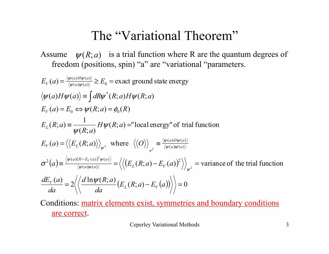
The “Variational Theorem” Assume is a trial function where R are the quantum degrees of
freedom (positions, spin) “a” are “variational “parameters.
Conditions: matrix elements exist, symmetries and boundary conditions
are correct.
);( aRψ
( ) ( ) ( )
( )( ) 0);();(ln2)(
function trial theof variance)();(
where);()(
function trialof energy" local");();(
1);(
)();()(
);();()()(
energy state groundexact )(
2
2
22
2)()(
)()()(2
)()()()(
00
*
0)()()()(
=−=
=−=≡
≡=
=≡
=⇔=
≡
=≥=
−
∫
aEaREda
aRddaadE
aEaREa
OaREaE
aRHaR
aRE
RaREaE
aRHaRdRaHa
EaE
VLV
VLaa
aaEHa
aaaOa
LV
L
V
aaaHa
V
V
ψ
σ
ψψ
φψ
ψψψψ
ψψψ
ψψ
ψψψψ
ψ
ψψψψ
ψ
Ceperley Variational Methods 4
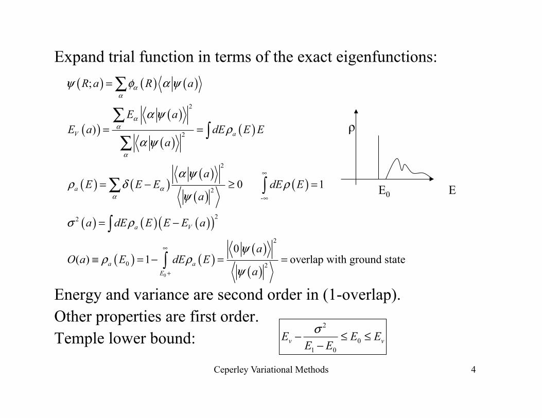
Expand trial function in terms of the exact eigenfunctions: Energy and variance are second order in (1-overlap). Other properties are first order. Temple lower bound:
( ) ( ) ( )
( )( )
( )( )
( ) ( )( )( )
( )
( ) ( ) ( )( )
( ) ( )( )( )0
2
2
2
2-
22
2
0 2
;
)
0 1
0( ) 1 overlap with ground state
V a
a
a V
a aE
R a R a
E aE a dE E E
a
aE E E dE E
a
a dE E E E a
aO a E dE E
a
αα
αα
α
αα
ψ φ α ψ
α ψρ
α ψ
α ψρ δ ρ
ψ
σ ρ
ψρ ρ
ψ
∞
∞
∞
+
=
= =
= − ≥ =
= −
≡ = − = =
∑
∑∫
∑
∑ ∫
∫
∫
E0 E
ρ
vv EEEE
E ≤≤−
− 001
2σ

Ceperley Variational Methods 10
Variational Monte Carlo (VMC)
• Variational Principle. Given an appropriate trial function: – Continuous – Proper symmetry – Normalizable – Finite variance
• Quantum chemistry uses a product of single particle functions
• With MC we can use any “computable” function.
– Sample R from |ψ|2 using MCMC. – Take average of local energy: – Optimize ψ to get the best upper bound
• Better wavefunction, lower variance! “Zero variance” principle. (non-classical)
ψ ψ
ψψ
ψ ψσ
ψψ
= ≥
= −
∫∫
∫∫
0
22 2
V
V
dR HE E
dR
dR HE
dR
2
1
0
( ) ( ) ( )
( )L
V L
E R R H R
E E R Eψ
ψ ψ−⎡ ⎤=ℜ⎣ ⎦= ≥
Ceperley Variational Methods 11
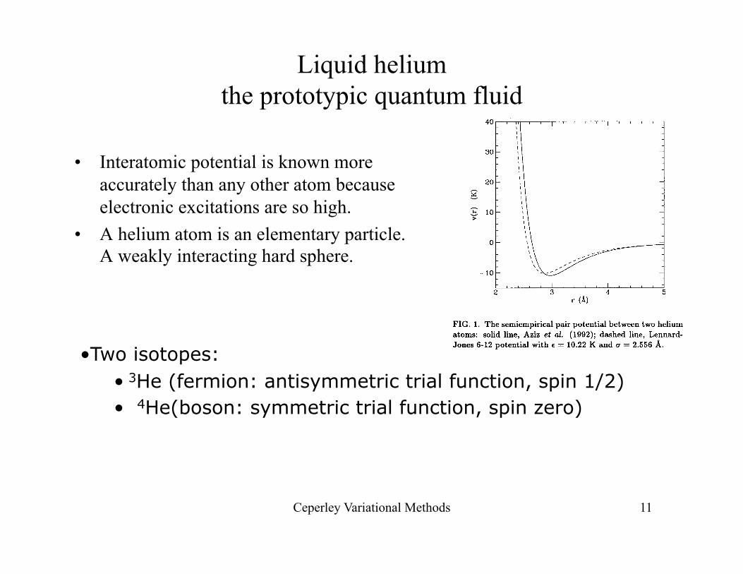
Liquid helium the prototypic quantum fluid
• Interatomic potential is known more accurately than any other atom because electronic excitations are so high.
• A helium atom is an elementary particle. A weakly interacting hard sphere.
• Two isotopes: • 3He (fermion: antisymmetric trial function, spin 1/2) • 4He(boson: symmetric trial function, spin zero)

Ceperley Variational Methods 13
Trial function for helium • We want finite variance of the local
energy. • Whenever 2 atoms get close together
wavefunction should vanish. • The pseudopotential u(r) is similar to
classical potential • Local energy has the form:
G is the pseudoforce: If v(r) diverges as r-n how should u(r)
diverge? Assume: U(r)=αr-m
Gives a cusp condition on u.
( )
2 2
( )
( ) ( ) 2 ( )
( )
iju r
i j
ij ij ii j i
i i ij
R e
E R v r u r G
G u r
ψ
ψ
λ λ
−
<
<
=
= − ∇ −
= ∇
∏
∑ ∑
∑
( )212 for 2
121
2
n mr mr n
nm
m
ε λ α
εαλ
− − −= >
= −
=2 1 2
2
12 u(r)= 2 '' '
'(0)2 ( 1)
De r u ur
euD
λ λ
λ
− −⎛ ⎞− = ∇ +⎜ ⎟⎝ ⎠
= −−

Ceperley Variational Methods 14
Optimization of trial function
• Try to optimize u(r) using reweighting
(correlated sampling) – Sample R using P(R)=ψ2(R,a0) – Now find minima of the analytic
function Ev(a) – Or minimize the variance (more
stable but wavefunctions less accurate).
• Statistical accuracy declines away from a0.
2
2
1
2
2
( ) ( )( )
( )
( , ) ( , )
( , )
( , )( , )
( )( , ) ( , ) ( , )
ψ ψ
ψ
ψ
ψ ψ−
=
=
=
=
⎡ ⎤⎢ ⎥⎣ ⎦=
∫∫
∑∑
∑∑
V
i ik
ik
i
ii
effi
i
a H aE a
a
w R a E R a
w R a
R aw R a
P RE R a R a H R a
wN
w

Ceperley Variational Methods 15
Other quantum properties • Kinetic energy • Potential energy • Pair correlation function • Structure function • Pressure (virial relation)
• Momentum distribution – Non-classical showing effects of
bose or fermi statistics – Fourier transform is the single
particle off-diagonal density matrix • Compute with McMillan Method. • Condensate fraction ~10%
Like properties from classical simulations No upper bound property Only first order in accuracy
*2 2 2
*2
2
( , ') ... ( , ...) ( ', ...)
( ', ,...)( , ,...)
Nn r r dr dr r r r r
r rr r
ψ ψ
ψψ
=
=
∫
Ceperley Variational Methods 17
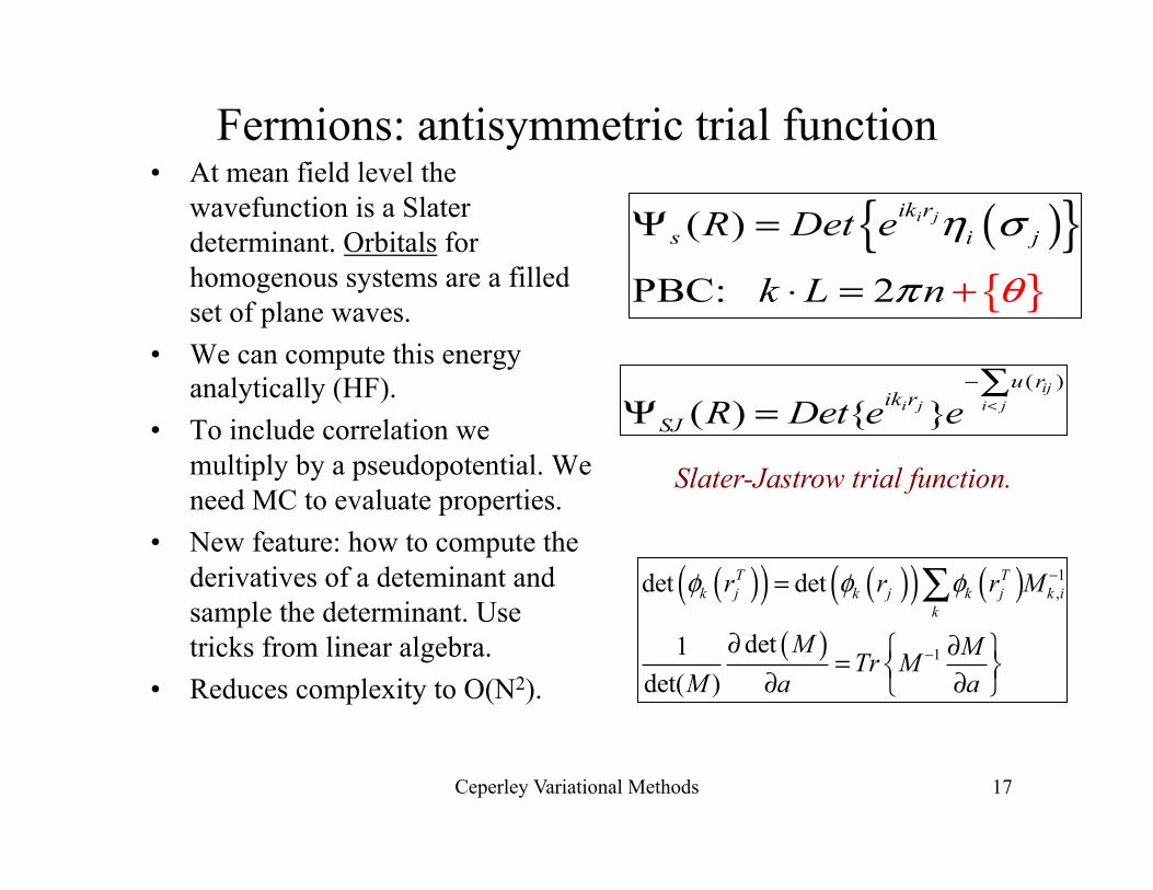
Fermions: antisymmetric trial function • At mean field level the
wavefunction is a Slater determinant. Orbitals for homogenous systems are a filled set of plane waves.
• We can compute this energy analytically (HF).
• To include correlation we multiply by a pseudopotential. We need MC to evaluate properties.
• New feature: how to compute the derivatives of a deteminant and sample the determinant. Use tricks from linear algebra.
• Reduces complexity to O(N2).
( ){ }{ }
( )
PBC: 2
i jik rs i jR Det e
k L n
η σ
π θ
Ψ =
⋅ = +
( )
( ) { }ij
i j i ju r
ik rSJ R Det e e <
−∑Ψ =
Slater-Jastrow trial function.
( )( ) ( )( ) ( )( )
1,
1
det det
det1det( )
T Tk j k j k j k i
kr r r M
M MTr MM a a
φ φ φ −
−
=
∂ ∂⎧ ⎫= ⎨ ⎬∂ ∂⎩ ⎭
∑

Ceperley Variational Methods 18
The electron gas D. M. Ceperley, Phys. Rev. B 18, 3126 (1978)
• Standard model for electrons in metals
• Basis of DFT. • Characterized by 2
dimensionless parameters: – Density – Temperature
• What is energy? • When does it freeze? • What is spin
polarization? • What are properties?
22 1
2 i
i i j ij
Hm r<
= − ∇ +∑ ∑h
02
/
/sr a ae Ta
=
Γ =
log( )Γ
log( )sr
Γ <Γ =
classical OCP175 classical meltingsr
Ceperley Variational Methods 19
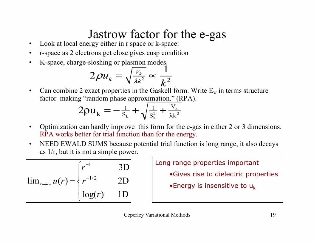
Jastrow factor for the e-gas • Look at local energy either in r space or k-space: • r-space as 2 electrons get close gives cusp condition • K-space, charge-sloshing or plasmon modes.
• Can combine 2 exact properties in the Gaskell form. Write EV in terms structure factor making “random phase approximation.” (RPA).
• Optimization can hardly improve this form for the e-gas in either 2 or 3 dimensions. RPA works better for trial function than for the energy.
• NEED EWALD SUMS because potential trial function is long range, it also decays as 1/r, but it is not a simple power.
2k
2kk k
VS1
S1
ku2 λ++−=ρ
2 2
12 kVk ku
kλρ = ∝
1
1/ 2
3Dlim ( ) 2D
log( ) 1Dr
ru r r
r
−
−→∞
⎧⎪= ⎨⎪⎩
Long range properties important
• Gives rise to dielectric properties
• Energy is insensitive to uk

Ceperley Variational Methods 20
Comparison of Trial functions • What do we choose for the trial function in VMC and DMC? • Slater-Jastrow (SJ) with plane wave orbitals :
• For higher accuracy we need to go beyond this form. • Include backflow-three body.
Example of incorrect physics within SJ
( )φ <
−∑Ψ =
( )
2( ) { }j
ij iji ju r
k rR Det e

Ceperley Variational Methods 21
Wavefunctions beyond Jastrow
• Use method of residuals construct a sequence of increasingly better trial wave functions.
• Zeroth order is Hartree-Fock wavefunction • First order is Slater-Jastrow pair wavefunction (RPA for electrons gives an
analytic formula) • Second order is 3-body backflow wavefunction • Three-body form is like a squared force. It is a bosonic term that does not
change the nodes.
>φφ<τ−+
−
φ≈φ n1n H
n1n e)R()R(
smoothing
ξΨ −∑ ∑ 22( )exp{ [ ( )( )] }ij ij i j
i jR r r r

Ceperley Variational Methods 22
Backflow- 3B Wave functions
• Backflow means change the coordinates to quasi- coordinates.
• Leads to a much improved energy
Kwon PRB 58, 6800 (1998).
{ } { }i j i ji iDet e Det e⇒k r k x
η= + −∑ ( )( )i i ij ij i jj
rx r r r
3DEG

Ceperley Variational Methods 23
Dependence of energy on wavefunction
3d Electron fluid at a density rs=10
Kwon, Ceperley, Martin, Phys. Rev. B58,6800, 1998
• Wavefunctions – Slater-Jastrow (SJ) – three-body (3) – backflow (BF) – fixed-node (FN)
• Energy <ψ |H| ψ> converges to ground state
• Variance <ψ [H-E]2ψ> to zero. • Using 3B-BF gains a factor of 4. • Using DMC gains a factor of 4.
-0.109
-0.1085
-0.108
-0.1075
-0.107
0 0.05 0.1
VarianceEnergy
FN -SJ
FN-BF
Ceperley Variational Methods 26
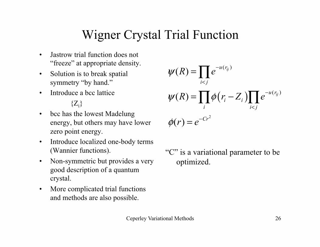
Wigner Crystal Trial Function • Jastrow trial function does not
“freeze” at appropriate density. • Solution is to break spatial
symmetry “by hand.” • Introduce a bcc lattice {Zi} • bcc has the lowest Madelung
energy, but others may have lower zero point energy.
• Introduce localized one-body terms (Wannier functions).
• Non-symmetric but provides a very good description of a quantum crystal.
• More complicated trial functions and methods are also possible.
“C” is a variational parameter to be optimized.
( )2
( )
( )
( )
( )
( )
ij
ij
u r
i j
u ri i
i i j
Cr
R e
R r Z e
r e
ψ
ψ φ
φ
−
<
−
<
−
=
= −
=
∏
∏ ∏

Ceperley Variational Methods 27
Twist averaged boundary conditions • In periodic boundary conditions (Γ
point), the wavefunction is periodicàLarge finite size effects for metals because of shell effects.
• Fermi liquid theory can be used to correct the properties.
• In twist averaged BC we use an arbitrary phase θ as r àr+L
• If one integrates over all phases the momentum distribution changes from a lattice of k-vectors to a fermi sea.
• Smaller finite size effects
Error with PBC Error with TABC
2
ikrekL nϕ
π θ== +
kx
( )3
3
( ) ( )12
ix L e x
A d A
θ
π
θ θπ
θπ −
Ψ + = Ψ
= Ψ Ψ∫

Ceperley Variational Methods 28
Twist averaged MC • Make twist vector dynamical by changing during the
random walk.
• Within GCE, change the number of electrons • Within TA-VMC
– Initialize twist vector. – Run usual VMC (with warmup) – Resample twist angle within cube – (iterate)
• Or do in parallel.
( ) i= 1,2,3iπ θ π− < ≤

Ceperley Variational Methods 30
Momentum Distribution • Momentum distribution
– Non-classical showing effects of bose or fermi statistics
– Fourier transform is the single particle off-diagonal density matrix
• Compute with McMillan Method.
*2 2 2
*2
2
1( , ') ... ( , ...) ( ', ...)
( , ...)( ', ...)
Nn r r dr dr r r r rZ
r rr r
ψ ψ
ψψ
=
=
∫
Ceperley Variational Methods 31
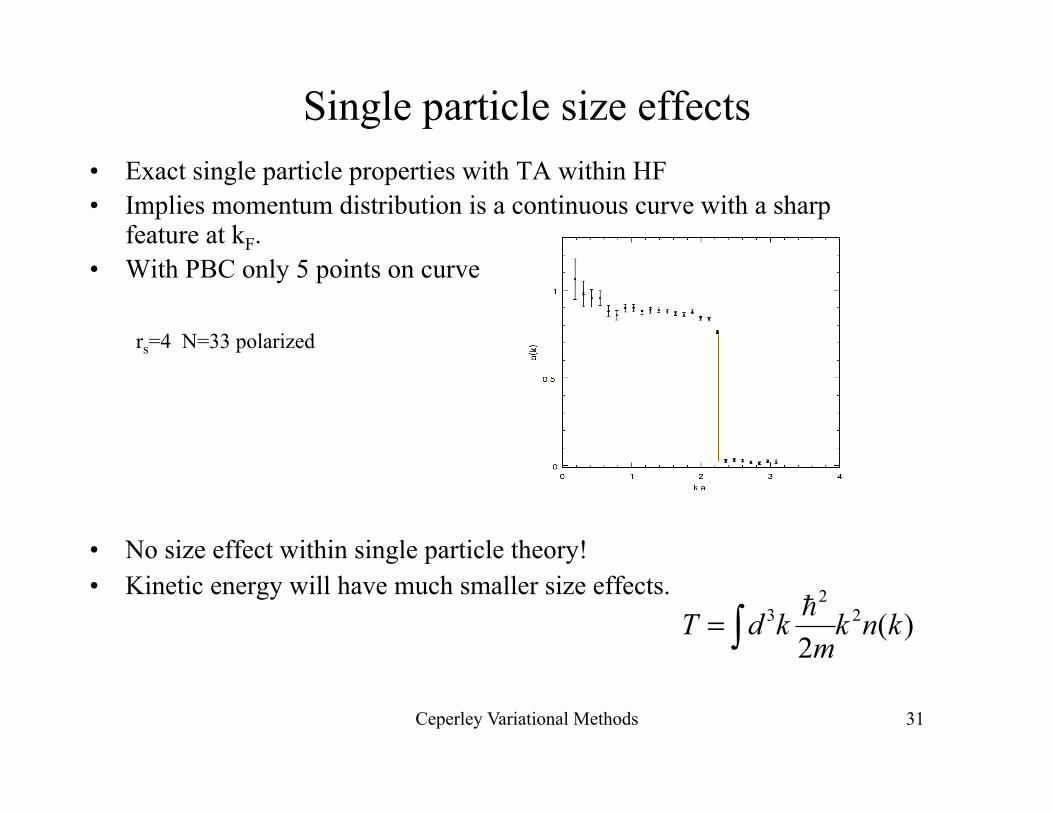
Single particle size effects • Exact single particle properties with TA within HF • Implies momentum distribution is a continuous curve with a sharp
feature at kF. • With PBC only 5 points on curve
rs=4 N=33 polarized
• No size effect within single particle theory! • Kinetic energy will have much smaller size effects.
)(2
22
3 knkm
kdT ∫=!

Ceperley Variational Methods 32
Potential energy • Write potential as integral over structure function:
• Error comes from 2 effects. – Approximating integral by sum – Finite size effects in S(k) at a given k.
• Within HF we get exact S(k) with TABC. • Discretization errors come only from non-analytic points of S(k).
– the absence of the k=0 term in sum. We can put it in by hand since we know the limit S(k) at small k (plasmon regime)
– Remaining size effects are smaller, coming from the non-analytic behavior of S(k) at 2kF.
1 2( )32
4 ( ) ( ) 1 ( 1) i r r kk kV d k S k S k N e
kπ ρ ρ −
−= = = + −∫
', '
2( ) 1HF q q kq q
S kN
δ − += − ∑

Ceperley Variational Methods 42
Summary of T=0 methods:
Variational(VMC), Fixed-node(FN), Released-node(RN)
1.E-05
1.E-04
1.E-03
1.E-02
1.E-01
1.E+00
1.E+01
1.E+00 1.E+01 1.E+02 1.E+03 1.E+04 1.E+05 1.E+06 1.E+07
computer time (sec)
erro
r (a
u)
Simple trial function
Better trial function
VMC FN
RN