The Variable-Order Fractional Calculus of VariationsThe fractional variational calculus is a recent...
136
arXiv:1805.00720v2 [math.OC] 17 Jun 2018 Ricardo Almeida, Dina Tavares, Delfim F. M. Torres The Variable-Order Fractional Calculus of Variations June 17, 2018 This is a preprint. The final authenticated version is available online as a SpringerBrief in Applied Sciences and Technology at: https://doi.org/10.1007/978-3-319-94006-9 Please cite this book as follows: R. Almeida, D. Tavares and D. F. M. Torres, The variable-order fractional calculus of variations, SpringerBriefs in Applied Sciences and Technology, Springer, Cham, 2019.
Transcript of The Variable-Order Fractional Calculus of VariationsThe fractional variational calculus is a recent...

arX
iv:1
805.
0072
0v2
[m
ath.
OC
] 1
7 Ju
n 20
18
Ricardo Almeida, Dina Tavares,
Delfim F. M. Torres
The Variable-Order Fractional
Calculus of Variations
June 17, 2018
This is a preprint. The final authenticated
version is available online as a SpringerBrief
in Applied Sciences and Technology at:
https://doi.org/10.1007/978-3-319-94006-9
Please cite this book as follows:
R. Almeida, D. Tavares and D. F. M. Torres,The variable-order fractional calculus of variations,SpringerBriefs in Applied Sciences and Technology, Springer, Cham, 2019.


Preface
This book intends to deepen the study of the fractional calculus, giving specialemphasis to variable-order operators.
Fractional calculus is a recent field of mathematical analysis and it is a gen-eralization of integer differential calculus, involving derivatives and integrals ofreal or complex order (Kilbas, Srivastava and Trujillo, 2006; Podlubny, 1999).The first note about this ideia of differentiation, for non-integer numbers, datesback to 1695, with a famous correspondence between Leibniz and L’Hopital.In a letter, L’Hopital asked Leibniz about the possibility of the order n in thenotation dny/dxn, for the nth derivative of the function y, to be a non-integer,n = 1/2. Since then, several mathematicians investigated this approach, likeLacroix, Fourier, Liouville, Riemann, Letnikov, Grunwald, Caputo, and con-tributed to the grown development of this field. Currently, this is one of themost intensively developing areas of mathematical analysis as a result of itsnumerous applications. The first book devoted to the fractional calculus waspublished by Oldham and Spanier in 1974, where the authors systematizedthe main ideas, methods and applications about this field (Mainardi, 2010).
In the recent years, fractional calculus has attracted the attention ofmany mathematicians, but also some researchers in other areas like physics,chemistry and engineering. As it is well known, several physical phenom-ena are often better described by fractional derivatives (Herrmann, 2013;Odzijewicz, Malinowska and Torres, 2012a; Sheng, 2012). This is mainly dueto the fact that fractional operators take into consideration the evolution ofthe system, by taking the global correlation, and not only local characteris-tics. Moreover, integer-order calculus sometimes contradict the experimentalresults and therefore derivatives of fractional order may be more suitable(Hilfer, 2000).
In 1993, Samko and Ross devoted themselves to investigate operatorswhen the order α is not a constant during the process, but variable on time:α(t) (Samko and Ross, 1993). An interesting recent generalization of the the-ory of fractional calculus is developed to allow the fractional order of thederivative to be non-constant, depending on time (Chen, Liu and Burrage,

VI
2014; Odzijewicz, Malinowska and Torres, 2012b, 2013a). With this approachof variable-order fractional calculus, the non-local properties are more evidentand numerous applications have been found in physics, mechanics, control andsignal processing (Coimbra, Soon and Kobayashi, 2005; Ingman and Suzdalnitsky,2004; Odzijewicz, Malinowska and Torres, 2013b; Ostalczyk et al., 2015; Ramirez and Coimbra,2011; Rapaic and Pisano, 2014; Valerio and Costa, 2013).
Although there are many definitions of fractional derivative, the mostcommonly used are the Riemann–Liouville, the Caputo, and the Grunwald-Letnikov derivatives. For more about the development of fractional calculus,we suggest (Samko, Kilbas and Marichev, 1993), (Samko and Ross, 1993),(Podlubny, 1999), (Kilbas, Srivastava and Trujillo, 2006) or (Mainardi, 2010).
One difficult issue that usually arises when dealing with such fractionaloperators, is the extreme difficulty in solving analytically such problems(Atangana and Cloot, 2013; Zhuang et al., 2009). Thus, in most cases, we donot know the exact solution for the problem and one needs to seek a numeri-cal approximation. Several numerical methods can be found in the literature,typically applying some discretization over time or replacing the fractional op-erators by a proper decomposition (Atangana and Cloot, 2013; Zhuang et al.,2009).
Recently, new approximation formulas were given for fractional constantorder operators, with the advantage that higher-order derivatives are not re-quired to obtain a good accuracy of the method (Atanackovic et al., 2013;Pooseh, Almeida and Torres, 2012, 2013). These decompositions only dependon integer-order derivatives, and by replacing the fractional operators thatappear in the problem by them, one leaves the fractional context ending upin the presence of a standard problem, where numerous tools are available tosolve them (Almeida, Pooseh and Torres, 2015).
The first goal of this book is to extend such decompositions to Caputo frac-tional problems of variable-order. For three types of Caputo derivatives withvariable-order, we obtain approximation formulas for the fractional operatorsand respective upper bounds for the errors.
Then, we focus our attention on a special operator introduced by Mali-nowska and Torres: the combined Caputo fractional derivative, which is an ex-tension of the left and the right fractional Caputo derivatives (Malinowska and Torres,2010). Considering α, β ∈ (0, 1) and γ ∈ [0, 1], the combined Caputo fractionalderivative operator CDα,β
γ is a convex combination of the left and the rightCaputo fractional derivatives, defined by
CDα,βγ = γ C
aDαt + (1− γ)Ct D
βb .
We consider this fractional operator with variable fractional order, i.e., thecombined Caputo fractional derivative of variable-order:
CDα(·,·),β(·,·)γ x(t) = γ1
CaD
α(·,·)t x(t) + γ2
Ct D
β(·,·)b x(t),
VII
where γ = (γ1, γ2) ∈ [0, 1]2, with γ1 and γ2 not both zero. With this fractionaloperator, we study different types of fractional calculus of variations problems,where the Lagrangian depends on the referred derivative.
The calculus of variations is a mathematical subject that appeared for-mally in the XVII century, with the solution to the bachistochrone problem,that deals with the extremization (minimization or maximization) of func-tionals (van Brunt, 2004). Usually, functionals are given by an integral thatinvolves one or more functions or/and its derivatives. This branch of mathe-matics has proved to be relevant because of the numerous applications existingin real situations.
The fractional variational calculus is a recent mathematical field that con-sists in minimizing or maximizing functionals that depend on fractional oper-ators (integrals or/and derivatives). This subject was introduced by Riewe in1996, where the author generalizes the classical calculus of variations, by usingfractional derivatives, and allows to obtain conservations laws with noncon-servative forces such as friction (Riewe, 1996, 1997). Later appeared severalworks on various aspects of the fractional calculus of variations and involv-ing different fractional operators, like the Riemann–Liouville, the Caputo,the Grunwald–Letnikov, the Weyl, the Marchaud or the Hadamard frac-tional derivatives (Agrawal, 2002; Almeida, 2016; Askari and Ansari, 2016;Atanackovic, Konjik and Pilipovic, 2008; Baleanu, 2008; Fraser, 1992; Georgieva and Guenther,2002; Jarad, Abdeljawad and Baleanu, 2010). For the state of the art of thefractional calculus of variations, we refer the readers to the books (Almeida, Pooseh and Torres,2015; Malinowska, Odzijewicz and Torres, 2015; Malinowska and Torres, 2012).
Specifically, here we study some problems of the calculus of variations withintegrands depending on the independent variable t, an arbitrary function x
and a fractional derivative CDα(·,·),β(·,·)γ x. The endpoint of the cost integral,
as well the terminal state, are considered to be free. The fractional problemof the calculus of variations consists in finding the maximizers or minimizersto the functional
J (x, T ) =
∫ T
a
L(
t, x(t),CDα(·,·),β(·,·)γ x(t)
)
dt+ φ(T, x(T )),
where CDα(·,·),β(·,·)γ x(t) stands for the combined Caputo fractional derivative
of variable fractional order, subject to the boundary condition x(a) = xa.For all variational problems presented here, we establish necessary optimalityconditions and transversality optimality conditions.
The book is organized in two parts, as follows. In the first part, we reviewthe basic concepts of fractional calculus (Chapter 1) and of the fractionalcalculus of variations (Chapter 2). In Chapter 1, we start with a brief overviewabout fractional calculus and an introduction to the theory of some specialfunctions in fractional calculus. Then, we recall several fractional operators(integrals and derivatives) definitions and some properties of the consideredfractional derivatives and integrals are introduced. In the end of this chapter,
VIII
we review integration by parts formulas for different operators. Chapter 2presents a short introduction to the classical calculus of variations and reviewdifferent variational problems, like the isoperimetric problems or problemswith variable endpoints. In the end of this chapter, we introduce the theory ofthe fractional calculus of variations and some fractional variational problemswith variable-order.
In the second part, we systematize some new recent results on variable-order fractional calculus of (Tavares, Almeida and Torres, 2015, 2016, 2017,2018a,b). In Chapter 3, considering three types of fractional Caputo deriva-tives of variable-order, we present new approximation formulas for those frac-tional derivatives and prove upper bound formulas for the errors. In Chapter 4,we introduce the combined Caputo fractional derivative of variable-order andcorresponding higher-order operators. Some properties are also given. Then,we prove fractional Euler–Lagrange equations for several types of fractionalproblems of the calculus of variations, with or without constraints.
References
Agrawal OP (2002) Formulation of Euler–Lagrange equations for fractionalvariational problems. J. Math. Anal. Appl. 272:368–379
Almeida R (2016) Fractional variational problems depending on indefiniteintegrals and with delay. Bull. Malays. Math. Sci. Soc. 39(4):1515–1528arXiv:1512.06752
Almeida R, Pooseh S, Torres DFM (2015) Computational Methods in theFractional Calculus of Variations. Imperial College Press, London
Askari H, Ansari A (2016) Fractional calculus of variations with a generalizedfractional derivative. Fract. Differ. Calc. 6:57–72
Atanackovic TM, Janev M, Pilipovic S, Zorica D (2013) An expansion formulafor fractional derivatives of variable order. Cent. Eur. J. Phys. 11(10):1350–1360
Atanackovic TM, Konjik S, Pilipovic S (2008) Variational problems withfractional derivatives: Euler–Lagrange equations. J. Phys. A 41(9):095201,12 pp
Atangana A, Cloot AH (2013) Stability and convergence of the space fractionalvariable-order Schrodinger equation. Adv. Difference Equ. 80(1):10 pp
Baleanu D (2008) New applications of fractional variational principles. Rep.Math. Phys. 61(2):199–206
Chen S, Liu F, Burrage K (2014) Numerical simulation of a newtwo–dimensional variable-order fractional percolation equation in non-homogeneous porous media. Comput. Math. Appl. 67(9):1673–1681
Coimbra CFM, Soon CM, Kobayashi MH (2005) The variable viscoelasticityoperator. Annalen der Physik 14(6):378–389
Fraser C (1992) Isoperimetric problems in variatonal calculus of Euler andLagrange. Historia Mathematica 19:4–23

References IX
Georgieva B, Guenther RB (2002) First Noether-type theorem for the gen-eralized variational principle of Herglotz. Topol. Methods Nonlinear Anal.20(2):261–273
Herrmann R (2013) Folded potentials in cluster physics–a comparison ofYukawa and Coulomb potentials with Riesz fractional integrals. J. Phys.A 46(40):405203, 12 pp
Hilfer R (2000) Applications of fractional calculus in physics. World Sci. Pub-lishing, River Edge, NJ
Ingman D, Suzdalnitsky J (2004) Control of damping oscillations by frac-tional differential operator with time–dependent order. Comput. Meth.Appl. Mech. Eng. 193(52):5585–5595
Jarad F, Abdeljawad T, Baleanu D (2010) Fractional variational principleswith delay within Caputo derivatives. Rep. Math. Phys. 65(1):17–28
Kilbas AA, Srivastava HM, Trujillo JJ (2006) Theory and Applications ofFractional Differential Equations. Elsevier, Amsterdam
Mainardi F (2010) Fractional Calculus and Waves in Linear Viscoelasticity.Imp. Coll. Press, London
Malinowska AB, Odzijewicz T, Torres DFM (2015) Advanced Methods in theFractional Calculus of Variations. Springer Briefs in Applied Sciences andTechnology, Springer, Cham
Malinowska AB, Torres DFM (2010) Fractional variational calculus in terms ofa combined Caputo derivative. Proceedings of FDA’10, The 4th IFACWork-shop on Fractional Differentiation and its Applications, Badajoz, Spain, Oc-tober 18–20, 2010 (Eds: I. Podlubny, B. M. Vinagre Jara, YQ. Chen, V. FeliuBatlle, I. Tejado Balsera):Article no. FDA10-084, 6 pp. arXiv:1007.0743
Malinowska AB, Torres DFM (2012) Introduction to the Fractional Calculusof Variations. Imp. Coll. Press, London
Odzijewicz T, Malinowska AB, Torres DFM (2012a) Fractional calculus ofvariations in terms of a generalized fractional integral with applications tophysics. Abstr. Appl. Anal. 2012:Art. ID 871912, 24 pp arXiv:1203.1961
Odzijewicz T, Malinowska AB, Torres DFM (2012b) Variable order fractionalvariational calculus for double integrals. Proceedings of the 51st IEEE Con-ference on Decision and Control, December 10–13, 2012, Maui, Hawaii:Art.no. 6426489, 6873–6878. arXiv:1209.1345
Odzijewicz T, Malinowska AB, Torres DFM (2013a) Fractional variationalcalculus of variable order. in Advances in harmonic analysis and operatortheory:291–301, Oper. Theory Adv. Appl., Birkhauser/Springer Basel AG,Basel arXiv:1110.4141
Odzijewicz T, Malinowska AB, Torres DFM (2013b) Noether’s theoremfor fractional variational problems of variable order. Cent. Eur. J. Phys.11(6):691–701 arXiv:1303.4075
Ostalczyk PW, Duch P, Brzezin ski DW, Sankowski D (2015) Order func-tions selection in the variable-, fractional-order PID controller. Advancesin Modelling and Control of Non–integer–Order Systems, Lecture Notes inElectrical Engineering 320:159–170.
X
Podlubny I (1999) Fractional Differential Equations. Academic Press, SanDiego, CA
Pooseh S, Almeida R, Torres DFM (2012) Approximation of fractional in-tegrals by means of derivatives. Comput. Math. Appl. 64(10):3090–3100arXiv:1201.5224
Pooseh S, Almeida R, Torres DFM (2013) Numerical approximations offractional derivatives with applications. Asian J. Control 15(3):698–712arXiv:1208.2588
Ramirez LES, Coimbra CFM (2011) On the variable order dynamics of thenonlinear wake caused by a sedimenting particle. Phys. D 240(13):1111–1118
Rapaic MR, Pisano A (2014) Variable-order fractional operators for adaptiveorder and parameter estimation. IEEE Trans. Automat. Control 59(3):798–803
Riewe F (1996) Nonconservative Lagrangian and Hamiltonian mechanics.Phys. Rev. E (3) 53(2):1890–1899
Riewe F (1997) Mechanics with fractional derivatives. Phys. Rev. E (3)55(3):3581–3592
Samko SG, Kilbas AA, Marichev OI (1993) Fractional Integrals and Deriva-tives. translated from the 1987 Russian original, Gordon and Breach, Yver-don
Samko SG, Ross B (1993) Integration and differentiation to a variable frac-tional order. Integral Transform. Spec. Funct. 1(4):277–300
Tavares D, Almeida R, Torres DFM (2015) Optimality conditions for frac-tional variational problems with dependence on a combined Caputo deriva-tive of variable order. Optimization 64(6):1381–1391 arXiv:1501.02082
Tavares D, Almeida R, Torres DFM (2016) Caputo derivatives of fractionalvariable order: numerical approximations. Commun. Nonlinear Sci. Numer.Simul. 35:69–87 arXiv:1511.02017
Tavares D, Almeida R, Torres DFM (2017) Constrained fractional variationalproblems of variable order. IEEE/CAA Journal Automatica Sinica 4(1):80–88 arXiv:1606.07512
Tavares D, Almeida R, Torres DFM (2018a) Fractional Herglotz variationalproblem of variable order. Disc. Contin. Dyn. Syst. Ser. S 11(1):143–154.arXiv:1703.09104
Tavares D, Almeida R, Torres DFM (2018b) Combined fractional variationalproblems of variable order and some computational aspects. J. Comput.Appl. Math. 339:374–388. arXiv:1704.06486
Valerio D, Costa JS (2013) Variable order fractional controllers. Asian J. Con-trol 15(3):648–657
van Brunt B (2004) The Calculus of Variations. Universitext, Springer, NewYork
Zheng B (2012) (G′/G)-expansion method for solving fractional partial dif-ferential equations in the theory of mathematical physics. Commun. Theor.Phys. 58(5):623–630

References XI
Zhuang P, Liu F, Anh V, Turner I (2009) Numerical methods for the variable-order fractional advection-diffusion equation with a nonlinear source term.SIAM J. Numer. Anal. 47(3):1760–1781.


Acknowledgements
This work was supported by Portuguese funds through the Center for Re-search and Development in Mathematics and Applications (CIDMA), and thePortuguese Foundation for Science and Technology (FCT), within projectUID/MAT/04106/2013.
Any comments or suggestions related to the material here contained aremore than welcome, and may be submitted by post or by electronic mail tothe authors:
Ricardo Almeida <[email protected]>
Center for Research and Development in Mathematics and ApplicationsDepartment of Mathematics, University of Aveiro3810-193 Aveiro, Portugal
Dina Tavares <[email protected]>ESECS, Polytechnic Institute of Leiria2410–272 Leiria, Portugal
Delfim F. M. Torres <[email protected]>Center for Research and Development in Mathematics and ApplicationsDepartment of Mathematics, University of Aveiro3810-193 Aveiro, Portugal

Contents
1 Fractional calculus . . . . . . . . . . . . . . . . . . . . . . . . . . . . . . . . . . . . . . . . . 11.1 Historical perspective . . . . . . . . . . . . . . . . . . . . . . . . . . . . . . . . . . . . 11.2 Special functions . . . . . . . . . . . . . . . . . . . . . . . . . . . . . . . . . . . . . . . . 41.3 Fractional integrals and derivatives . . . . . . . . . . . . . . . . . . . . . . . . 5
1.3.1 Classical operators . . . . . . . . . . . . . . . . . . . . . . . . . . . . . . . . 61.3.2 Some properties of the Caputo derivative . . . . . . . . . . . . . 91.3.3 Combined Caputo derivative . . . . . . . . . . . . . . . . . . . . . . . . 111.3.4 Variable-order operators . . . . . . . . . . . . . . . . . . . . . . . . . . . . 121.3.5 Generalized fractional operators . . . . . . . . . . . . . . . . . . . . . 141.3.6 Integration by parts . . . . . . . . . . . . . . . . . . . . . . . . . . . . . . . 16
2 The calculus of variations . . . . . . . . . . . . . . . . . . . . . . . . . . . . . . . . . . 212.1 The classical calculus of variations . . . . . . . . . . . . . . . . . . . . . . . . . 21
2.1.1 Euler–Lagrange equations . . . . . . . . . . . . . . . . . . . . . . . . . . 232.1.2 Problems with variable endpoints . . . . . . . . . . . . . . . . . . . . 242.1.3 Constrained variational problems . . . . . . . . . . . . . . . . . . . . 25
2.2 Fractional calculus of variations . . . . . . . . . . . . . . . . . . . . . . . . . . . 262.2.1 Fractional Euler–Lagrange equations . . . . . . . . . . . . . . . . . 272.2.2 Fractional variational problems of variable-order . . . . . . . 29
3 Expansion formulas for fractional derivatives . . . . . . . . . . . . . . 353.1 Caputo-type fractional operators of variable-order . . . . . . . . . . . 35
3.1.1 Caputo derivatives for functions of one variable . . . . . . . 363.1.2 Caputo derivatives for functions of several variables . . . . 42
3.2 Numerical approximations . . . . . . . . . . . . . . . . . . . . . . . . . . . . . . . . 453.3 Example . . . . . . . . . . . . . . . . . . . . . . . . . . . . . . . . . . . . . . . . . . . . . . . 543.4 Applications . . . . . . . . . . . . . . . . . . . . . . . . . . . . . . . . . . . . . . . . . . . . 54
3.4.1 A time-fractional diffusion equation . . . . . . . . . . . . . . . . . . 553.4.2 A fractional partial differential equation in fluid
mechanics . . . . . . . . . . . . . . . . . . . . . . . . . . . . . . . . . . . . . . . . 58

XVI Contents
4 The fractional calculus of variations . . . . . . . . . . . . . . . . . . . . . . . 614.1 Introduction . . . . . . . . . . . . . . . . . . . . . . . . . . . . . . . . . . . . . . . . . . . . 62
4.1.1 Combined operators of variable-order . . . . . . . . . . . . . . . . 624.1.2 Generalized fractional integration by parts . . . . . . . . . . . . 66
4.2 Fundamental variational problem . . . . . . . . . . . . . . . . . . . . . . . . . . 684.2.1 Necessary optimality conditions . . . . . . . . . . . . . . . . . . . . . 684.2.2 Particular cases . . . . . . . . . . . . . . . . . . . . . . . . . . . . . . . . . . . 734.2.3 Examples . . . . . . . . . . . . . . . . . . . . . . . . . . . . . . . . . . . . . . . . 74
4.3 Higher-order variational problems . . . . . . . . . . . . . . . . . . . . . . . . . 754.3.1 Necessary optimality conditions . . . . . . . . . . . . . . . . . . . . . 754.3.2 Example . . . . . . . . . . . . . . . . . . . . . . . . . . . . . . . . . . . . . . . . . 82
4.4 Variational problems with time delay . . . . . . . . . . . . . . . . . . . . . . 824.4.1 Necessary optimality conditions . . . . . . . . . . . . . . . . . . . . . 834.4.2 Example . . . . . . . . . . . . . . . . . . . . . . . . . . . . . . . . . . . . . . . . . 86
4.5 Isoperimetric problems . . . . . . . . . . . . . . . . . . . . . . . . . . . . . . . . . . . 864.5.1 Necessary optimality conditions I . . . . . . . . . . . . . . . . . . . . 874.5.2 Necessary optimality conditions II . . . . . . . . . . . . . . . . . . . 924.5.3 Example . . . . . . . . . . . . . . . . . . . . . . . . . . . . . . . . . . . . . . . . . 94
4.6 Variational problems with holonomic constraints . . . . . . . . . . . . 954.6.1 Necessary optimality conditions . . . . . . . . . . . . . . . . . . . . . 964.6.2 Example . . . . . . . . . . . . . . . . . . . . . . . . . . . . . . . . . . . . . . . . . 100
4.7 Fractional variational Herglotz problem . . . . . . . . . . . . . . . . . . . . 1004.7.1 Fundamental problem of Herglotz . . . . . . . . . . . . . . . . . . . 1014.7.2 Several independent variables . . . . . . . . . . . . . . . . . . . . . . . 1044.7.3 Examples . . . . . . . . . . . . . . . . . . . . . . . . . . . . . . . . . . . . . . . . 108
Appendix
Index . . . . . . . . . . . . . . . . . . . . . . . . . . . . . . . . . . . . . . . . . . . . . . . . . . . . . . . . . . 121

1
Fractional calculus
In this chapter, a brief introduction to the theory of fractional calculus ispresented. We start with a historical perspective of the theory, with a strongconnection with the development of classical calculus (Section 1.1). Then,in Section 1.2, we review some definitions and properties about a few specialfunctions that will be needed. We end with a review on fractional integralsand fractional derivatives of noninteger order and with some formulas of in-tegration by parts, involving fractional operators (Section 1.3).
The content of this chapter can be found in some classical books on frac-tional calculus, for example (Almeida, Pooseh and Torres, 2015; Kilbas, Srivastava and Trujillo,2006; Malinowska and Torres, 2012a; Podlubny, 1999; Samko, Kilbas and Marichev,1993).
1.1 Historical perspective
Fractional Calculus (FC) is considered as a branch of mathematical analysiswhich deals with the investigation and applications of integrals and deriva-tives of arbitrary order. Therefore, FC is an extension of the integer-ordercalculus that considers integrals and derivatives of any real or complex order(Kilbas, Srivastava and Trujillo, 2006; Samko, Kilbas and Marichev, 1993),i.e., unify and generalize the notions of integer-order differentiation and n-fold integration.
FC was born in 1695 with a letter that L’Hopital wrote to Leibniz, wherethe derivative of order 1/2 is suggested (Oldham and Spanier, 1974). AfterLeibniz had introduced in his publications the notation for the nth derivativeof a function y,
dny
dxn,
L’Hopital wrote a letter to Leibniz to ask him about the possibility of aderivative of integer order to be extended in order to have a meaning whenthe order is a fraction: ”What if n be 1/2?” (Ross, 1977). In his answer, dated
2 1 Fractional calculus
on 30 September 1695, Leibniz replied that ”This is an apparent paradox fromwhich, one day, useful consequences will be drawn” and, today, we know it istruth. Then, Leibniz still wrote about derivatives of general order and in 1730,Euler investigated the result of the derivative when the order n is a fraction.But, only in 1819, with Lacroix, appeared the first definition of fractionalderivative based on the expression for the nth derivative of the power function.Considering y = xm, with m a positive integer, Lacroix developed the nthderivative
dny
dxn=
m!
(m− n)!xm−n, m ≥ n,
and using the definition of Gamma function, for the generalized factorial, hegot
dny
dxn=
Γ (m+ 1)
Γ (m− n+ 1)xm−n.
Lacroix also studied the following example, for n = 12 and m = 1:
d1/2x
dx1/2=
Γ (2)
Γ (3/2)x
12 =
2√x√π. (1.1)
Since then, many mathematicians, like Fourier, Abel, Riemann, Liouville,among others, contributed to the development of this subject. One of thefirst applications of fractional calculus appear in 1823 by Niels Abel, throughthe solution of an integral equation of the form
∫ t
0
(t− τ)−αx(τ)dτ = k,
used in the formulation of the Tautochrone problem (Abel, 1923; Ross, 1977).
Different forms of fractional operators have been introduced along time,like the Riemann–Liouville, the Grunwald-Letnikov, the Weyl, the Caputo, theMarchaud or the Hadamard fractional derivatives (Kilbas, Srivastava and Trujillo,2006; Oldham and Spanier, 1974; Oliveira and Machado, 2014; Podlubny,1999). The first approach is the Riemann-Liouville, which is based on iterat-ing the classical integral operator n times and then considering the Cauchy’sformula where n! is replaced by the Gamma function and hence the fractionalintegral of noninteger order is defined. Then, using this operator, some of thefractional derivatives mentioned above are defined.
During three centuries, FC was developed but as a pure theoretical sub-ject of mathematics. In recent times, FC had an increasing of importancedue to its applications in various fields, not only in mathematics, but also inphysics, mechanics, engineering, chemistry, biology, finance, and others ar-eas of science (Herrmann, 2013; Hilfer, 2000; Li and Liu, 2016; Mainardi,2010; Odzijewicz, Malinowska and Torres, 2013c; Pinto and Carvalho, 2014;

1.1 Historical perspective 3
Sierociuk et al., 2015; Sun, Chen and Chen, 2009). In some of these appli-cations, many real world phenomena are better described by noninteger or-der derivatives, if we compare with the usual integer-order calculus. In fact,fractional order derivatives have unique characteristics that may model cer-tain dynamics more efficiently. Firstly, we can consider any real order for thederivatives, and thus we are not restricted to integer order derivatives only;secondly, they are nonlocal operators, in opposite to the usual derivatives,thus containing memory. With the memory property, one can take into ac-count the past of the processes. Signal processing, modeling and control aresome areas that have been the object of more intensive publishing in the lastdecades.
In most applications of the FC, the order of the derivative is assumed to befixed along the process, that is, when determining what is the order α > 0 suchthat the solution of the fractional differential equationDαy(t) = f(t, y(t)) bet-ter approaches the experimental data, we consider the order α to be a fixedconstant. Of course, this may not be the best option, since trajectories are adynamic process, and the order may vary. More interesting possibilities arisewhen one considers the order α of the fractional integrals and derivatives notconstant during the process but to be a function α(t), depending on time.Then, we may seek what is the best function α(·) such that the variable-orderfractional differential equation Dα(t)y(t) = f(t, y(t)) better describes the pro-cess under study. This approach is very recent. One such fractional calcu-lus of variable-order was introduced in (Samko and Ross, 1993). Afterwards,several mathematicians obtained important results about variable-order frac-tional calculus, and some applications appeared, like in mechanics, in themodeling of linear and nonlinear viscoelasticity oscillators and in other phe-nomena where the order of the derivative varies with time. See, for instance,(Almeida and Torres, 2013; Atanackovic and Pilipovic, 2011; Coimbra, 2003;Odzijewicz, Malinowska and Torres, 2013a; Ramirez and Coimbra, 2011; Samko,1995; Sheng et al., 2011).
The most common fractional operators considered in the literature takeinto account the past of the process. They are usually called left fractionaloperators. But in some cases we may be also interested in the future of theprocess, and the computation of α(t) to be influenced by it. In that case, rightfractional derivatives are then considered. Recently, in some works, the maingoal is to develop a theory where both fractional operators are taken into ac-count. For that, some combined fractional operators are introduced, like thesymmetric fractional derivative, the Riesz fractional integral and derivative,the Riesz–Caputo fractional derivative and the combined Caputo fractionalderivative that consists in a linear combination of the left and right frac-tional operators. For studies with fixed fractional order, see (Klimek, 2001;Malinowska and Torres, 2011, 2012a,b).
Due to the growing number of applications of fractional calculus in scienceand engineering, numerical approaches are being developed to provide tools forsolving such problems. At present, there are already vast studies on numerical
4 1 Fractional calculus
approximate formulas (Kumar, Pandey and Sharma, 2017; Li, Chen and Ye,2011). For example, for numerical modeling of time fractional diffusion equa-tions, we refer the reader to (Fu, Chen and Yang, 2013).
1.2 Special functions
Before introducing the basic facts on fractional operators, we recall four typesof functions that are important in Fractional Calculus: the Gamma, Psi, Betaand Mittag-Leffler functions. Some properties of these functions are also re-called.
Definition 1 The Euler Gamma function is an extension of the factorialfunction to real numbers, and it is defined by
Γ (t) =
∫ ∞
0
τ t−1 exp(−τ) dτ, t > 0.
For example, Γ (1) = 1, Γ (2) = 1 and Γ (3/2) =√π2 . For positive integers
n, we get Γ (n) = (n− 1)!. We mention that other definitions for the Gammafunction exist, and it is possible to define it for complex numbers, except forthe non-positive integers.
The Gamma function is considered the most important Eulerian functionused in fractional calculus, because it appears in almost every fractional inte-gral and derivative definitions. A basic but fundamental property of Γ , thatwe will use later, is obtained using integration by parts:
Γ (t+ 1) = t Γ (t).
Definition 2 The Psi function is the derivative of the logarithm of theGamma function:
Ψ(t) =d
dtln (Γ (t)) =
Γ ′(t)
Γ (t).
The follow function is used sometimes for convenience to replace a com-bination of Gamma functions. It is important in FC because it shares a formthat is similar to the fractional derivative or integral of many functions, par-ticularly power functions.
Definition 3 The Beta function B is defined by
B(t, u) =
∫ 1
0
st−1(1− s)u−1ds, t, u > 0.
This function satisfies an important property:
B(t, u) =Γ (t)Γ (u)
Γ (t+ u).

1.3 Fractional integrals and derivatives 5
With this property, it is obvious that the Beta function is symmetric, i.e.,
B(t, u) = B(u, t).
The next function is a direct generalization of the exponential series and itwas defined by the mathematician Mittag-Leffler in 1903 (Podlubny, 1999).
Definition 4 Let α > 0. The function Eα defined by
Eα(t) =
∞∑
k=0
tk
Γ (αk + 1), t ∈ R,
is called the one parameter Mittag-Leffler function.
For α = 1, this function coincides with the series expansion of et, i.e.,
E1(t) =
∞∑
k=0
tk
Γ (k + 1)=
∞∑
k=0
tk
k!= et.
While linear ordinary differential equations present in general the exponentialfunction as a solution, the Mitttag-Leffler function occurs naturally in the solu-tion of fractional order differential equations (Kilbas, Srivastava and Trujillo,2006). For this reason, in recent times, the Mittag-Leffler function has be-come an important function in the theory of the fractional calculus and itsapplications.
It is also common to represent the Mittag-Leffler function in two argu-ments. This generalization of Mittag-Leffler function was studied by Wimanin 1905 (Mainardi, 2010).
Definition 5 The two-parameter function of the Mittag-Leffler type with pa-rameters α, β > 0 is defined by
Eα,β(t) =
∞∑
k=0
tk
Γ (αk + β), t ∈ R.
If β = 1, this function coincides with the classical Mittag-Leffler function,i.e., Eα,1(t) = Eα(t).
1.3 Fractional integrals and derivatives
In this section, we recall some definitions of fractional integral and fractionaldifferential operators, that includes all we use throughout this book. In theend, we present some integration by parts formulas because they have a crucialrole in deriving Euler–Lagrange equations.

6 1 Fractional calculus
1.3.1 Classical operators
As it was seen in Section 1.1, there are more than one way to generalize integer-order operations to the non-integer case. Here, we present several definitionsand properties about fractional operators, omitting some details about theconditions that ensure the existence of such fractional operators.
In general, the fractional derivatives are defined using fractional integrals.We present only two fractional integrals operators, but there are several knownforms of the fractional integrals.
Let x : [a, b] → R be an integrable function and α > 0 a real number.Starting with Cauchy’s formula for a n-fold iterated integral, given by
aInt x(t) =
∫ t
a
dτ1
∫ τ1
a
dτ2 · · ·∫ τn−1
a
x(τn)dτn
=1
(n− 1)!
∫ t
a
(t− τ)n−1x(τ)dτ,
(1.2)
where n ∈ N, Liouville and Riemann defined fractional integration, generaliz-ing equation (1.2) to noninteger values of n and using the definition of Gammafunction Γ . With this, we introduce two important concepts: the left and theright Riemann–Liouville fractional integrals.
Definition 6 We define the left and right Riemann–Liouville fractional in-tegrals of order α, respectively, by
aItαx(t) =
1
Γ (α)
∫ t
a
(t− τ)α−1x(τ)dτ, t > a
and
tIbαx(t) =
1
Γ (α)
∫ b
t
(τ − t)α−1x(τ)dτ, t < b.
The constants a and b determine, respectively, the lower and upper bound-ary of the integral domain. Additionally, if x is a continuous function, asα → 0, aIt
α = tIbα = I, with I the identity operator, i.e., aIt
αx(t) =
tIbαx(t) = x(t).We present the second fractional integral operator, introduced by J.
Hadamard in 1892 (Kilbas, Srivastava and Trujillo, 2006).
Definition 7 We define the left and right Hadamard fractional integrals oforder α, respectively, by
aJαt x(t) =
1
Γ (α)
∫ t
a
(
lnt
τ
)α−1x(τ)
τdτ, t > a
and
tJαb x(t) =
1
Γ (α)
∫ b
t
(
lnτ
t
)α−1 x(τ)
τdτ, t < b.

1.3 Fractional integrals and derivatives 7
The three most frequently used definitions for fractional derivatives are:the Grunwald-Letnikov, the Riemann–Liouville and the Caputo fractionalderivatives (Oldham and Spanier, 1974; Podlubny, 1999). Other definitionswere introduced by others mathematicians, as for instance Weyl, Fourier,Cauchy, Abel.
Let x ∈ AC([a, b];R) be an absolutely continuous functions on the interval[a, b], and α a positive real number. Using Definition 6 of Riemann–Liouvillefractional integrals, we define the left and the right Riemann–Liouville andCaputo derivatives as follows.
Definition 8 We define the left and right Riemann–Liouville fractional deriva-tives of order α > 0, respectively, by
aDαt x(t) =
(
d
dt
)n
aIn−αt x(t)
=1
Γ (n− α)
(
d
dt
)n ∫ t
a
(t− τ)n−α−1x(τ)dτ, t > a
and
tDαb x(t) =
(
− d
dt
)n
tIn−αb x(t)
=(−1)n
Γ (n− α)
(
d
dt
)n ∫ b
t
(τ − t)n−α−1x(τ)dτ, t < b,
where n = [α] + 1.
The following definition was introduced in (Caputo, 1967). The Caputofractional derivatives, in general, are more applicable and interesting in fieldslike physics and engineering, for its properties like the initial conditions.
Definition 9 We define the left and right Caputo fractional derivatives oforder α, respectively, by
CaD
αt x(t) = aI
n−αt
(
d
dt
)n
x(t)
=1
Γ (n− α)
∫ t
a
(t− τ)n−α−1x(n)(τ)dτ, t > a
and
Ct D
αb x(t) = tI
n−αb
(
− d
dt
)n
x(t)
=(−1)n
Γ (n− α)
∫ b
t
(τ − t)n−α−1x(n)(τ)dτ, t < b,
where n = [α] + 1 if α /∈ N and n = α if α ∈ N.

8 1 Fractional calculus
Obviously, the above defined operators are linear. From these definitions,it is clear that the Caputo fractional derivative of a constant C is zero, which isfalse when we consider the Riemann–Liouville fractional derivative. If x(t) =C, with C a constant, then we get
CaD
αt x(t) =
Ct D
αb x(t) = 0
and
aDαt x(t) =
C (t− a)−α
Γ (1− α), tD
αb x(t) =
C (b − t)−α
Γ (1− α).
For this reason, in some applications, Caputo fractional derivatives seem tobe more natural than the Riemann–Liouville fractional derivatives.
Remark 1 If α goes to n−, with n ∈ N, then the fractional operators intro-duced above coincide with the standard derivatives:
aDαt = C
aDαt =
(
d
dt
)n
and
tDαb = C
t Dαb =
(
− d
dt
)n
.
The Riemann–Liouville fractional integral and differential operators of or-der α > 0 of power functions return power functions, as we can see below.
Lemma 2 Let x be the power function x(t) = (t− a)γ . Then, we have
aIαt x(t) =
Γ (γ + 1)
Γ (γ + α+ 1)(t− a)γ+α, γ > −1
and
aDαt x(t) =
Γ (γ + 1)
Γ (γ − α+ 1)(t− a)γ−α, γ > −1.
In particular, if we consider γ = 1, a = 0 and α = 1/2, then the left
Riemann–Liouville fractional derivative of x(t) = t is 2√t√π, the same result
(1.1) as Lacroix obtained in 1819.Grunwald and Letnikov, respectively in 1867 and 1868, returned to the
original sources and started the formulation by the fundamental definition ofa derivative, as a limit,
x(1)(t) = limh→0
x(t+ h)− x(t)
h
and considering the iteration at the nth order derivative formula:
x(n)(t) = limh→0
1
hn
n∑
k=0
(−1)k(
n
k
)
x(t− kh), n ∈ N, (1.3)

1.3 Fractional integrals and derivatives 9
where(
nk
)
= n(n−1)(n−2)...(n−k+1)k! , with n, k ∈ N, the usual notation for the
binomial coefficients. The Grunwald-Letnikov definition of fractional deriva-tive consists in a generalization of (1.3) to derivatives of arbitrary order α(Podlubny, 1999).
Definition 10 The αth order Grunwald-Letnikov fractional derivative offunction x is given by
GLa Dα
t x(t) = limh−→0
h−αn∑
k=0
(−1)k(
α
k
)
x(t− kh),
where(
αk
)
= Γ (α+1)k!Γ (α−k+1) and nh = t− a.
Lemma 3 Let x be the power function x(t) = (t − a)γ , where γ is a realnumber. Then, for 0 < α < 1 and γ > 0, we have
GLa Dα
t x(t) =Γ (γ + 1)
Γ (γ − α+ 1)(t− a)γ−α.
Definition 11 We define the left and right Hadamard fractional derivativesof order α, respectively, by
aDαt x(t) =
(
td
dt
)n1
Γ (n− α)
∫ t
a
(
lnt
τ
)n−α−1x(τ)
τdτ
and
tDαb x(t) =
(
−t ddt
)n1
Γ (n− α)
∫ b
t
(
lnτ
t
)n−α−1 x(τ)
τdτ,
for all t ∈ (a, b), where n = [α] + 1.
Observe that, for all types of derivative operators, if variable t is the time-variable, the left fractional derivative of x is interpreted as a past state of theprocess, while the right fractional derivative of x is interpreted as a futurestate of the process.
1.3.2 Some properties of the Caputo derivative
For α > 0 and x ∈ AC([a, b];R), the Riemann–Liouville and Caputo deriva-tives are related by the following formulas (Kilbas, Srivastava and Trujillo,2006):
CaD
αt x(t) = aD
αt
[
x(t) −n−1∑
k=0
x(k)(a)(t− a)k
k!
]
(1.4)
and
Ct D
αb x(t) = tD
αb
[
x(t) −n−1∑
k=0
x(k)(b)(b− t)k
k!
]
, (1.5)

10 1 Fractional calculus
where n = [α] + 1 if α /∈ N and n = α if α ∈ N.In particular, when α ∈ (0, 1), the relations (1.4) and (1.5) take the form:
CaD
αt x(t) = aD
αt (x(t)− x(a))
= aDαt x(t)− x(a)
Γ (1−α) (t− a)−α (1.6)
andCt D
αb x(t) = tD
αb (x(t)− x(b))
= tDαb x(t)−
x(b)Γ (1−α) (b − t)−α.
(1.7)
It follows from (1.6) and (1.7) that the left Riemann–Liouville derivativeequals the left Caputo fractional derivative in the case x(a) = 0 and theanalogue holds for the right derivatives under the assumption x(b) = 0.
In Theorem 4, we see that the Caputo fractional derivatives providesa left inverse operator to the Riemann–Liouville fractional integration (cf.Lemma 2.21 in (Kilbas, Srivastava and Trujillo, 2006)).
Theorem 4 Let α > 0 and let x ∈ C ([a, b];Rn). For Caputo fractional oper-ators, the next rules hold:
CaD
αt aI
αt x(t) = x(t)
andCt D
αb tI
αb x(t) = x(t).
The next statement characterizes the composition of the Riemann–Liouvillefractional integration operators with the Caputo fractional differentiation op-erators (cf. Lemma 2.22 in (Kilbas, Srivastava and Trujillo, 2006)).
Theorem 5 Let α > 0. If x ∈ ACn ([a, b];R), then
aIαt
CaD
αt x(t) = x(t) −
n−1∑
k=0
x(k)(a)
k!(t− a)k
and
tIαb
Ct D
αb x(t) = x(t)−
n−1∑
k=0
(−1)kx(k)(b)
k!(b− t)k,
with n = [α] + 1 if α /∈ N and n = α if α ∈ N.In particular, when α ∈ (0, 1), then
aIαt
CaD
αt x(t) = x(t)− x(a) and tI
αb
Ct D
αb x(t) = x(t)− x(b).
Similarly to the Riemann–Liouville fractional derivative, the Caputo frac-tional derivative of a power function yields a power function of the same form.
1.3 Fractional integrals and derivatives 11
Lemma 6 Let α > 0. Then, the following relations hold:
CaD
αt (t− a)γ =
Γ (γ + 1)
Γ (γ − α+ 1)(t− a)γ−α, γ > n− 1
andCt D
αb (b− t)γ =
Γ (γ + 1)
Γ (γ − α+ 1)(b− t)γ−α, γ > n− 1,
with n = [α] + 1 if α /∈ N and n = α if α ∈ N.
1.3.3 Combined Caputo derivative
In this section, we introduce a special operator for our work, the combinedCaputo fractional derivative. We extend the notion of the Caputo fractionalderivative to the fractional derivative CDα,β
γ , that involves the left and theright Caputo fractional derivative, i.e., it combines the past and the future ofthe process into one single operator.
This operator was introduced in (Malinowska and Torres, 2010), mo-tivated by the ideia of the symmetric fractional derivative introduced in(Klimek, 2001):
Definition 12 Considering the left and right Riemann–Liouville derivatives,the symmetric fractional derivative is given by
aDαb x(t) =
1
2[aD
αt x(t) + tD
αb x(t)] . (1.8)
Other combined operators were studied. For example, we have the Rieszand the Riesz–Caputo operators (Malinowska and Torres, 2012a).
Definition 13 Let x : [a, b] → R be a function of class C1 and α ∈ (0, 1).For t ∈ [a, b], the Riesz fractional integral of order α, is defined by
Ra I
αb x(t) =
1
2Γ (α)
∫ b
a
|t− τ |α−1x(τ)dτ
=1
2[aI
αt x(t) + tI
αb x(t)] ,
and the Riesz fractional derivative of order α, is defined by
RaD
αb x(t) =
1
Γ (1− α)
d
dt
∫ b
a
|t− τ |−αx(τ)dτ
=1
2[aD
αt x(t)− tD
αb x(t)] .
Definition 14 Considering the left and right Caputo derivatives, Riesz–Caputo fractional derivative is given by
12 1 Fractional calculus
RCa Dα
b x(t) =1
Γ (1− α)
∫ b
a
|t− τ |−α d
dτx(τ)dτ
=1
2
[
CaD
αt x(t)− C
t Dαb x(t)
]
.
(1.9)
Remark 7 (Malinowska and Torres (2012a)) If α goes to 1, then thefractional derivatives introduced above coincide with the standard derivative:
RaD
αb = RC
a Dαb =
d
dt.
Similarly to the last operator (1.9), the combined Caputo derivative is aconvex combination of the left and the right Caputo fractional derivatives.But, in this operator, we also consider other coefficients for the convex combi-nation besides 1/2. Moreover, the orders α and β of the left- and right-sidedfractional derivatives can be different. Therefore, the combined Caputo deriva-tive is a convex combination of the left Caputo fractional derivative of orderα and the right Caputo fractional derivative of order β.
Definition 15 Let α, β ∈ (0, 1) and γ ∈ [0, 1]. The combined Caputo frac-tional derivative operator CDα,β
γ is defined by
CDα,βγ = γ C
aDαt + (1− γ)Ct D
βb , (1.10)
which acts on x ∈ AC ([a, b];R) in the following way:
CDα,βγ x(t) = γ C
aDαt x(t) + (1− γ)Ct D
βb x(t).
The operator (1.10) is obviously linear. Observe that
CDα,β0 = C
t Dβb and CDα,β
1 = CaD
αt .
The symmetric fractional derivative and the Riesz fractional derivative areuseful tools to describe some nonconservative models. But those types of dif-ferentiation do not seem suitable for all kinds of variational problems becausethey are based on the Riemann–Liouville fractional derivatives and thereforethe possibility that admissible trajectories x have continuous fractional deriva-tives imply that x(a) = x(b) = 0 (Samko and Ross, 1993). For more detailsabout the combined Caputo fractional derivative, see (Malinowska and Torres,2011, 2012b,c; Odzijewicz, Malinowska and Torres, 2012b).
1.3.4 Variable-order operators
Very useful physical applications have given birth to the variable-order frac-tional calculus, for example in modeling mechanical behaviors (Fu, Chen and Yang,2013; Sun et al., 2013). Nowadays, variable-order fractional calculus is partic-ularly recognized as a useful and promising approach in the modelling of

1.3 Fractional integrals and derivatives 13
diffusion processes, in order to characterize time-dependent or concentration-dependent anomalous diffusion, or diffusion processes in inhomogeneous porousmedia (Sun et al., 2012).
Now, we present the fundamental notions of the fractional calculus ofvariable-order (Malinowska, Odzijewicz and Torres, 2015). We consider thefractional order of the derivative and of the integral to be a continuous functionof two variables, α(·, ·) with domain [a, b]2, taking values on the open interval(0, 1). Let x : [a, b] → R be a function.
First, we recall the generalization of fractional integrals for a variable-orderα(·, ·).Definition 16 The left and right Riemann–Liouville fractional integrals oforder α(·, ·) are defined by
aIα(·,·)t x(t) =
∫ t
a
1
Γ (α(t, τ))(t− τ)α(t,τ)−1x(τ)dτ, t > a
and
tIα(·,·)b x(t) =
∫ b
t
1
Γ (α(τ, t))(τ − t)α(τ,t)−1x(τ)dτ, t < b,
respectively.
We remark that, in contrast to the fixed fractional order case, variable-order fractional integrals are not the inverse operation of the variable-orderfractional derivatives.
For fractional derivatives, we consider two types: the Riemann–Liouvilleand the Caputo fractional derivatives.
Definition 17 The left and right Riemann–Liouville fractional derivatives oforder α(·, ·) are defined by
aDα(·,·)t x(t) =
d
dtaI
α(·,·)t x(t)
=d
dt
∫ t
a
1
Γ (1− α(t, τ))(t− τ)−α(t,τ)x(τ)dτ, t > a
(1.11)
and
tDα(·,·)b x(t) =− d
dttI
α(·,·)b x(t)
=d
dt
∫ b
t
−1
Γ (1− α(τ, t))(τ − t)−α(τ,t)x(τ)dτ, t < b
(1.12)
respectively.
Lemma 8 gives a Riemann–Liouville variable-order fractional integral andfractional derivative for the power function x(t) = (t− a)γ , where we assumethat the fractional order depends only on the first variable: α(t, τ) := α(t),where α : [a, b] → (0, 1) is a given function.
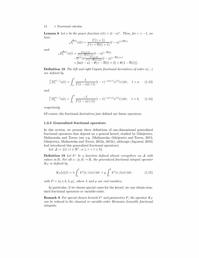
14 1 Fractional calculus
Lemma 8 Let x be the power function x(t) = (t−a)γ . Then, for γ > −1, wehave
aIα(t)t x(t) =
Γ (γ + 1)
Γ (γ + α(t) + 1)(t− a)γ+α(t)
and
aDα(t)t x(t) = Γ (γ+1)
Γ (γ−α(t)+1)(t− a)γ−α(t)
−α(1)(t) Γ (γ+1)Γ (γ−α(t)+2) (t− a)γ−α(t)+1
× [ln(t− a)− Ψ(γ − α(t) + 2) + Ψ(1 − α(t))] .
Definition 18 The left and right Caputo fractional derivatives of order α(·, ·)are defined by
CaD
α(·,·)t x(t) =
∫ t
a
1
Γ (1− α(t, τ))(t− τ)−α(t,τ)x(1)(τ)dτ, t > a (1.13)
and
Ct D
α(·,·)b x(t) =
∫ b
t
−1
Γ (1− α(τ, t))(τ − t)−α(τ,t)x(1)(τ)dτ, t < b, (1.14)
respectively.
Of course, the fractional derivatives just defined are linear operators.
1.3.5 Generalized fractional operators
In this section, we present three definitions of one-dimensional generalizedfractional operators that depend on a general kernel, studied by Odzijewicz,Malinowska and Torres (see e.g. (Malinowska, Odzijewicz and Torres, 2015;Odzijewicz, Malinowska and Torres, 2012a, 2013c), although (Agrawal, 2010)had introduced this generalized fractional operators).
Let ∆ := (t, τ) ∈ R2 : a ≤ τ < t ≤ b.
Definition 19 Let kα be a function defined almost everywhere on ∆ withvalues in R. For all x : [a, b] → R, the generalized fractional integral operatorKP is defined by
KP [x](t) = λ
∫ t
a
kα(t, τ)x(τ)dτ + µ
∫ b
t
kα(τ, t)x(τ)dτ, (1.15)
with P = 〈a, t, b, λ, µ〉, where λ and µ are real numbers.
In particular, if we choose special cases for the kernel, we can obtain stan-dard fractional operators or variable-order.
Remark 9 For special chosen kernels kα and parameters P , the operator KP
can be reduced to the classical or variable-order Riemann–Liouville fractionalintegrals:
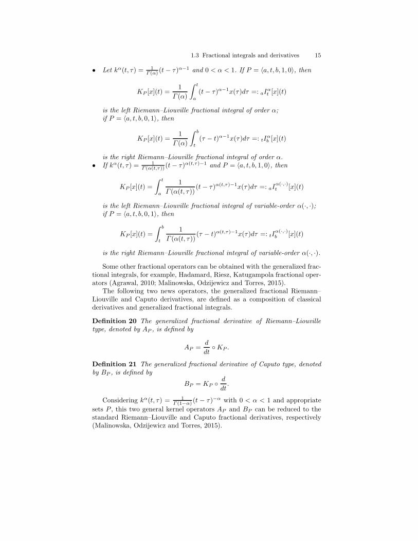
1.3 Fractional integrals and derivatives 15
• Let kα(t, τ) = 1Γ (α) (t− τ)α−1 and 0 < α < 1. If P = 〈a, t, b, 1, 0〉, then
KP [x](t) =1
Γ (α)
∫ t
a
(t− τ)α−1x(τ)dτ =: aIαt [x](t)
is the left Riemann–Liouville fractional integral of order α;if P = 〈a, t, b, 0, 1〉, then
KP [x](t) =1
Γ (α)
∫ b
t
(τ − t)α−1x(τ)dτ =: tIαb [x](t)
is the right Riemann–Liouville fractional integral of order α.• If kα(t, τ) = 1
Γ (α(t,τ))(t− τ)α(t,τ)−1 and P = 〈a, t, b, 1, 0〉, then
KP [x](t) =
∫ t
a
1
Γ (α(t, τ))(t− τ)α(t,τ)−1x(τ)dτ =: aI
α(·,·)t [x](t)
is the left Riemann–Liouville fractional integral of variable-order α(·, ·);if P = 〈a, t, b, 0, 1〉, then
KP [x](t) =
∫ b
t
1
Γ (α(t, τ))(τ − t)α(t,τ)−1x(τ)dτ =: tI
α(·,·)b [x](t)
is the right Riemann–Liouville fractional integral of variable-order α(·, ·).
Some other fractional operators can be obtained with the generalized frac-tional integrals, for example, Hadamard, Riesz, Katugampola fractional oper-ators (Agrawal, 2010; Malinowska, Odzijewicz and Torres, 2015).
The following two news operators, the generalized fractional Riemann–Liouville and Caputo derivatives, are defined as a composition of classicalderivatives and generalized fractional integrals.
Definition 20 The generalized fractional derivative of Riemann–Liouvilletype, denoted by AP , is defined by
AP =d
dtKP .
Definition 21 The generalized fractional derivative of Caputo type, denotedby BP , is defined by
BP = KP d
dt.
Considering kα(t, τ) = 1Γ (1−α) (t − τ)−α with 0 < α < 1 and appropriate
sets P , this two general kernel operators AP and BP can be reduced to thestandard Riemann–Liouville and Caputo fractional derivatives, respectively(Malinowska, Odzijewicz and Torres, 2015).

16 1 Fractional calculus
1.3.6 Integration by parts
In this section, we summarize formulas of integration by parts because theyare important results to find necessary optimality conditions when dealingwith variational problems.
First, we present the rule of fractional integration by parts for theRiemann–Liouville fractional integral.
Theorem 10 Let 0 < α < 1, p ≥ 1, q ≥ 1 and 1/p + 1/q ≤ 1 + α. If y ∈Lp([a, b];R) and x ∈ Lq([a, b];R), then the following formula for integrationby parts hold:
∫ b
a
y(t) aIαt x(t)dt =
∫ b
a
x(t) tIαb y(t)dt.
For Caputo fractional derivatives, the integration by parts formulas arepresented below (Almeida and Malinowska, 2013).
Theorem 11 Let 0 < α < 1. The following relations hold:
∫ b
a
y(t)CaDαt x(t)dt =
∫ b
a
x(t) tDαb y(t)dt+
[
x(t) tI1−αb y(t)
]t=b
t=a(1.16)
and
∫ b
a
y(t)Ct Dαb x(t)dt =
∫ b
a
x(t) aDαt y(t)dt−
[
x(t) aI1−αt y(t)
]t=b
t=a. (1.17)
When α → 1, we get CaD
αt = aD
αt = d
dt ,Ct D
αb = tD
αb = − d
dt , aIαt = tI
αb =
I, and formulas (1.16) and (1.17) give the classical formulas of integration byparts.
Then, we introduce the integration by parts formulas for variable-orderfractional integrals (Odzijewicz, Malinowska and Torres, 2013b).
Theorem 12 Let 1n < α(t, τ) < 1 for all t, τ ∈ [a, b] and a certain n ∈ N
greater or equal than two, and x, y ∈ C([a, b];R). Then the following formulafor integration by parts hold:
∫ b
a
y(t) aIα(·,·)t x(t)dt =
∫ b
a
x(t) tIα(·,·)b y(t)dt.
In the following theorem, we present the formulas involving the Ca-puto fractional derivative of variable-order. The theorem was proved in(Odzijewicz, Malinowska and Torres, 2013b) and gives a generalization of thestandard fractional formulas of integration by parts for a constant α.
Theorem 13 Let 0 < α(t, τ) < 1− 1n for all t, τ ∈ [a, b] and a certain n ∈ N
greater or equal than two. If x, y ∈ C1 ([a, b];R), then the fractional integrationby parts formulas

References 17
∫ b
a
y(t)CaDα(·,·)t x(t)dt =
∫ b
a
x(t) tDα(·,·)b y(t)dt+
[
x(t) tI1−α(·,·)b y(t)
]t=b
t=a
and∫ b
a
y(t)Ct Dα(·,·)b x(t)dt =
∫ b
a
x(t) aDα(·,·)t y(t)dt−
[
x(t) aI1−α(·,·)t y(t)
]t=b
t=a
hold.
This last theorem have an important role in this work to the proof of thegeneralized Euler–Lagrange equations.
In the end of this chapter, we present integration by parts formulas forgeneralized fractional operators (Malinowska, Odzijewicz and Torres, 2015).For that, we need the following definition:
Definition 22 Let P = 〈a, t, b, λ, µ〉. We denote by P ∗ the parameter setP ∗ = 〈a, t, b, µ, λ〉. The parameter P ∗ is called the dual of P .
Let 1 < p <∞ and q be the adjoint of p, that is 1p +
1q = 1. A proof of the
next result can be found in (Malinowska, Odzijewicz and Torres, 2015).
Theorem 14 Let k ∈ Lq(∆;R). Then the operator KP∗ is a linear boundedoperator from Lp([a, b];R) to Lq([a, b];R). Moreover, the following integrationby parts formula holds:
∫ b
a
x(t) ·KP [y](t)dt =
∫ b
a
y(t) ·KP∗ [x](t)dt
for all x, y ∈ Lp([a, b];R).
References
Abel NH (1823) Solution de quelques problemes a l’aide d’integrales definies.Mag. Naturv. 1(2):1–127
Agrawal OP (2010) Generalized variational problems and Euler-Lagrangeequations. Comput. Math. Appl. 59(5):1852–1864
Almeida R, Malinowska AB (2013) Generalized transversality conditions infractional calculus of variations. Commun. Nonlinear Sci. Numer. Simul.18(3):443–452
Almeida R, Pooseh S, Torres DFM (2015) Computational Methods in theFractional Calculus of Variations. Imperial College Press, London
Almeida R, Torres DFM (2013) An expansion formula with higher-orderderivatives for fractional operators of variable order. The Scientific WorldJournal 2013 Art. ID 915437, 11 pp arXiv:1309.4899
Atanackovic TM, Pilipovic S (2011) Hamilton’s principle with variable orderfractional derivatives. Fract. Calc. Appl. Anal. 14:94–109
18 1 Fractional calculus
Caputo M (1967) Linear model of dissipation whose Q is almost frequencyindependent–II. Geophys. J. R. Astr. Soc. 13:529–539
Coimbra CFM (2003) Mechanics with variable-order differential operators.Ann. Phys. 12(11–12):692–703
Fu Z-J, Chen W, Yang H-T (2013) Boundary particle method for Laplacetransformed time fractional diffusion equations. J. Comput. Phys. 235:52–66
Herrmann R (2013) Folded potentials in cluster physics–a comparison ofYukawa and Coulomb potentials with Riesz fractional integrals. J. Phys.A 46(40):405203, 12 pp
Hilfer R (2000) Applications of fractional calculus in physics. World Sci. Pub-lishing, River Edge, NJ
Kilbas AA, Srivastava HM, Trujillo JJ (2006) Theory and Applications ofFractional Differential Equations. Elsevier, Amsterdam
Klimek M (2001) Fractional sequential mechanics – models with symmetricfractional derivative. Czechoslovak J. Phys. 51(12):1348–1354
Kumar K, Pandey R, Sharma S (2017) Comparative study of three numeri-cal schemes for fractional integro–differential equations. J. Comput. Appl.Math. 315:287–302
Li CP, Chen A, Ye J (2011) Numerical approaches to fractional calculus andfractional ordinary differential equation. J. Comput. Phys. 230(9):3352–3368
Li G, Liu H (2016) Stability analysis and synchronization for a class offractional-order neural networks. Entropy 18(55):13 pp
Mainardi F (2010) Fractional Calculus and Waves in Linear Viscoelasticity.Imp. Coll. Press, London
Malinowska AB, Odzijewicz T, Torres DFM (2015) Advanced Methods in theFractional Calculus of Variations. Springer Briefs in Applied Sciences andTechnology, Springer, Cham
Malinowska AB, Torres DFM (2010) Fractional variational calculus in terms ofa combined Caputo derivative. Proceedings of FDA’10, The 4th IFACWork-shop on Fractional Differentiation and its Applications, Badajoz, Spain, Oc-tober 18–20, 2010 (Eds: I. Podlubny, B. M. Vinagre Jara, YQ. Chen, V. FeliuBatlle, I. Tejado Balsera):Article no. FDA10-084, 6 pp. arXiv:1007.0743
Malinowska AB, Torres DFM (2011) Fractional calculus of variations fora combined Caputo derivative. Fract. Calc. Appl. Anal. 14(4):523–537arXiv:1109.4664
Malinowska AB, Torres DFM (2012a) Introduction to the Fractional Calculusof Variations. Imp. Coll. Press, London
Malinowska AB, Torres DFM (2012b) Multiobjective fractional variationalcalculus in terms of a combined Caputo derivative. Appl. Math. Comput.218(9):5099–5111 arXiv:1110.6666
Malinowska AB, Torres DFM (2012c) Towards a combined fractionalmechanics and quantization. Fract. Calc. Appl. Anal. 15(3):407–417arXiv:1206.0864
References 19
Odzijewicz T, Malinowska AB, Torres DFM (2012a) Fractional calculus ofvariations in terms of a generalized fractional integral with applications tophysics. Abstr. Appl. Anal. 2012:Art. ID 871912, 24 pp arXiv:1203.1961
Odzijewicz T, Malinowska AB, Torres DFM (2012b) Fractional variationalcalculus with classical and combined Caputo derivatives. Nonlinear Anal.75(3):1507–1515 arXiv:1101.2932
Odzijewicz T, Malinowska AB, Torres DFM (2013a) Fractional variationalcalculus of variable order. in Advances in harmonic analysis and operatortheory:291–301, Oper. Theory Adv. Appl., Birkhauser/Springer Basel AG,Basel arXiv:1110.4141
Odzijewicz T, Malinowska AB, Torres DFM (2013b) Noether’s theoremfor fractional variational problems of variable order. Cent. Eur. J. Phys.11(6):691–701 arXiv:1303.4075
Odzijewicz T, Malinowska AB, Torres DFM (2013c) A generalized fractionalcalculus of variations. Control Cybernet. 42(2):443–458 arXiv:1304.5282
Oldham KB, Spanier J (1974) The Fractional Calculus. Academic Press, NewYork
Oliveira EC, Machado JAT (2014) A Review of definitions for fractionalderivatives and integral. Math. Probl. in Eng. 2014:238459, 6 pp
Pinto C, Carvalho ARM (2014) New findings on the dynamics of HIV andTB coinfection models. Appl. Math. Comput. 242:36–46
Podlubny I (1999) Fractional Differential Equations. Academic Press, SanDiego, CA
Ramirez LES, Coimbra CFM (2011) On the variable order dynamics of thenonlinear wake caused by a sedimenting particle. Phys. D 240(13):1111–1118
Ross B (1977) The development of fractional calculus 1695–1900. HistoriaMathematica 4:75–89
Samko SG (1995) Fractional integration and differentiation of variable order.Anal. Math. 21(3):213–236
Samko SG, Kilbas AA, Marichev OI (1993) Fractional Integrals and Deriva-tives. translated from the 1987 Russian original, Gordon and Breach, Yver-don
Samko SG, Ross B (1993) Integration and differentiation to a variable frac-tional order. Integral Transform. Spec. Funct. 1(4):277–300
Sheng H, Sun HG, Coopmans C, Chen YQ, Bohannan GW (2011) A physicalexperimental study of variable-order fractional integrator and differentiator.Eur. Phys. J. 193(1):93–104
Sierociuk D, Skovranek T, Macias M, Podlubny I, Petras I, Dzielinski A,Ziubinski P (2015) Diffusion process modeling by using fractional–ordermodels. Appl. Math. Comput. 257(15):2–11
Sun HG, Chen W, Chen YQ (2009) Variable order fractional differential op-erators in anomalous diffusion modeling. Physica A. 388(21):4586–4592
20 1 Fractional calculus
Sun H, Chen W, Li C, Chen Y (2012) Finite difference schemes for variable-order time fractional diffusion equation. Internat. J. Bifur. Chaos Appl. Sci.Engrg. 22(4):1250085, 16 pp
Sun H, Hu S, Chen Y, Chen W, Yu Z (2013) A dynamic-order fractionaldynamic system. Chinese Phys. Lett. 30(4):046601, 4 pp

2
The calculus of variations
As part of this book is devoted to the fractional calculus of variations, inthis chapter we introduce the basic concepts about the classical calculus ofvariations and the fractional calculus of variations. The study of fractionalproblems of the calculus of variations and respective Euler–Lagrange typeequations is a subject of current strong research.
In Section 2.1, we introduce some concepts and important results fromthe classical theory. Afterwards, in Section 2.2, we start with a brief historicalintroduction to the non–integer calculus of variations and then we presentrecent results on the fractional calculus of variations.
For more information about this subject, we refer the reader to the books(Almeida, Pooseh and Torres, 2015; Malinowska, Odzijewicz and Torres, 2015;Malinowska and Torres, 2012; van Brunt, 2004).
2.1 The classical calculus of variations
The calculus of variations is a field of mathematical analysis that concernswith finding extrema (maxima or minima) for functionals, i.e., concerns withthe problem of finding a function for which the value of a certain integral iseither the largest or the smallest possible.
In this context, a functional is a mapping from a set of functions to thereal numbers, i.e., it receives a function and produces a real number. LetD ⊆ C2([a, b];R) be a linear space endowed with a norm ‖ · ‖. The costfunctional J : D → R is generally of the form
J (x) =
∫ b
a
L (t, x(t), x′(t)) dt, (2.1)
where t ∈ [a, b] is the independent variable, usually called time, and x(t) ∈ R
is a function. The integrand L : [a, b]×R2 → R, that depends on the function
22 2 The calculus of variations
x, its derivative x′ and the independent variable t, is a real-valued function,called the Lagrangian.
The roots of the calculus of variations appear in works of Greek thinkers,such as Queen Dido or Aristotle in the late of the 1st century BC. During the17th century, some physicists and mathematicians (Galileo, Fermat, Newton,among others) investigated some variational problems, but in general they didnot use variational methods to solve them. The development of the calculus ofvariations began with a problem posed by Johann Bernoulli in 1696, called thebrachistochrone problem: given two points A and B in a vertical plane, what isthe curve traced out by a point acted on only by gravity, which starts at A andreaches B in minimal time? The curve that solves the problem is called thebrachistochrone. This problem caught the attention of some mathematiciansincluding Jakob Bernoulli, Leibniz, L’Hopital and Newton, which presentedalso a solution for the brachistochrone problem. Integer variational calculus isstill, nowadays, a revelant area of research. It plays a significant role in manyareas of science, physics, engineering, economics, and applied mathematics.
The classical variational problem, considered by Leonhard Euler, is statedas follows.Let a, b ∈ R. Among all functions x ∈ D, find the ones that minimize (ormaximize) the functional J : D → R, where
J (x) =
∫ b
a
L (t, x(t), x′(t)) dt, (2.2)
subject to the boundary conditions
x(a) = xa, x(b) = xb, (2.3)
with xa, xb fixed reals and the Lagrangian L satisfying some smoothness prop-erties. Usually, we say that a function is ”sufficiently smooth” for a particulardevelopment if all required actions (integration, differentiation, . . .) are pos-sible.
Definition 23 A trajectory x ∈ C2([a, b];R) is said to be an admissible tra-jectory if it satisfies all the constraints of the problem along the interval [a, b].The set of admissible trajectories is denoted by D.
To discuss maxima and minima of functionals, we need to introduce thefollowing definition.
Definition 24 We say that x⋆ ∈ D is a local extremizer to the functionalJ : D → R if there exists some real ǫ > 0, such that
∀x ∈ D : ‖x⋆ − x‖ < ǫ ⇒ J (x⋆)− J (x) ≤ 0 ∨ J (x⋆)− J (x) ≥ 0.
In this context, as we are dealing with functionals defined on functions,we need to clarify the term of directional derivatives, here called variations.The concept of variation of a functional is central to obtain the solution ofvariational problems.

2.1 The classical calculus of variations 23
Definition 25 Let J be defined on D. The first variation of a functional Jat x ∈ D in the direction h ∈ D is defined by
δJ (x, h) = limǫ→0
J (x+ ǫh)− J (x)
ǫ=
d
dǫJ (x + ǫh)
]
ǫ=0
,
where x and h are functions and ǫ is a scalar, whenever the limit exists.
Definition 26 A direction h ∈ D, h 6= 0, is said to be an admissible variationfor J at y ∈ D if
1. δJ (x, h) exists;2. x+ ǫh ∈ D for all sufficiently small ǫ.
With the condition that J (x) be a local extremum and the definitionof variation, we have the following result that offers a necessary optimalitycondition for problems of calculus of variations (van Brunt, 2004).
Theorem 15 Let J be a functional defined on D. If x⋆ minimizes (or max-imizes) the functional J over all functions x : [a, b] → R satisfying boundaryconditions (2.3), then
δJ (x⋆, h) = 0
for all admissible variations h at x⋆.
2.1.1 Euler–Lagrange equations
Although the calculus of variations was born with Johann’s problem, it waswith the work of Euler in 1742 and the one of Lagrange in 1755 that a system-atic theory was developed. The common procedure to address such variationalproblems consists in solving a differential equation, called the Euler–Lagrangeequation, which every minimizer/maximizer of the functional must satisfy.
In Lemma 16, we review an important result to transform the necessarycondition of extremum in a differential equation, free of integration with anarbitrary function. In literature, it is known as the fundamental lemma of thecalculus of variations.
Lemma 16 Let x be continuous in [a, b] an let h be an arbitrary function on[a, b] such that it is continuous and h(a) = h(b) = 0. If
∫ b
a
x(t)h(t)dt = 0
for all such h, then x(t) = 0 for all t ∈ [a, b].
For the sequel, we denote by ∂iz, i ∈ 1, 2, . . . ,M, with M ∈ N, thepartial derivative of a function z : RM → R with respect to its ith argument.Now we can formulate the necessary optimality condition for the classicalvariational problem (van Brunt, 2004).
24 2 The calculus of variations
Theorem 17 If x is an extremizing of the functional (2.2) on D, subject to(2.3), then x satisfies
∂2L (t, x(t), x′(t))− d
dt∂3L (t, x(t), x′(t)) = 0 (2.4)
for all t ∈ [a, b].
To solve this second order differential equation, the two given boundaryconditions (2.3) provide sufficient information to determine the two arbitraryconstants.
Definition 27 A curve x that is a solution of the Euler–Lagrange differentialequation will be called an extremal of J .
2.1.2 Problems with variable endpoints
In the basic variational problem considered previously, the functional J tominimize (or maximize) is subject to given boundary conditions of the form
x(a) = xa, x(b) = xb,
where xa, xb ∈ R are fixed. It means that the solution of the problem, x, needsto pass through the prescribed points. This variational problem is called a fixedendpoints variational problem. The Euler–Lagrange equation (2.4) is normallya second-order differential equation containing two arbitrary constants, sowith two given boundary conditions provided, they are sufficient to determinethe two constants.
However, in some areas, like physics and geometry, the variational prob-lems do not impose the appropriate number of boundary conditions. In thesecases, when one or both boundary conditions are missing, that is, when theset of admissible functions may take any value at one or both of the bound-aries, then one or two auxiliary conditions, known as the natural boundaryconditions or transversality conditions, need to be obtained in order to solvethe equation (van Brunt, 2004):
[
∂L(t, x(t), x′(t))
∂x′
]
t=a
= 0 and/or
[
∂L(t, x(t), x′(t))
∂x′
]
t=b
= 0. (2.5)
There are different types of variational problems with variable endpoints:
• Free terminal point – one boundary condition at the initial time (x(a) =xa). The terminal point is free (x(b) ∈ R);
• Free initial point – one boundary condition at the final time (x(b) = xb).The initial point is free (x(a) ∈ R);
• Free endpoints – both endpoints are free (x(a) ∈ R, x(b) ∈ R);• Variable endpoints – the initial point x(a) or/and the endpoint x(b) is
variable on a certain set, for example, on a prescribed curve.

2.1 The classical calculus of variations 25
Another generalization of the variational problem consists to find an opti-mal curve x and the optimal final time T of the variational integral, T ∈ [a, b].This problem is known in the literature as a free-time problem (Chiang, 1992).An example is the following free-time problem with free terminal point. LetD denote the subset C2([a, b];R) × [a, b] endowed with a norm ‖(·, ·)‖. Findthe local minimizers of the functional J : D → R, with
J (x, T ) =
∫ T
a
L(t, x(t), x′(t))dt, (2.6)
over all (x, T ) ∈ D satisfying the boundary condition x(a) = xa, with xa ∈ R
fixed. The terminal time T and the terminal state x(T ) are here both free.
Definition 28 We say that (x⋆, T ⋆) ∈ D is a local extremizer (minimizer ormaximizer) to the functional J : D → R as in (2.6) if there exists some ǫ > 0such that, for all (x, T ) ∈ D,
‖(x⋆, T ⋆)− (x, T )‖ < ǫ⇒ J(x⋆, T ⋆) ≤ J(x, T ) ∨ J(x⋆, T ⋆) ≥ J(x, T ).
To develop a necessary optimality condition to problem (2.6) for an ex-tremizer (x⋆, T ⋆), we need to consider an admissible variation of the form:
(x⋆ + ǫh, T ⋆ + ǫ∆T ),
where h ∈ C1([a, b];R) is a perturbing curve that satisfies the conditionh(a) = 0, ǫ represents a small real number, and ∆T represents an arbitrarilychosen small change in T . Considering the functional J (x, T ) in this admissi-ble variation, we get a function of ǫ, where the upper limit of integration willalso vary with ǫ:
J (x⋆ + ǫh, T ⋆ + ǫ∆T ) =
∫ T⋆+ǫ∆T
a
L(t, (x⋆ + ǫh)(t), (x⋆ + ǫh)′(t))dt. (2.7)
To find the first-order necessary optimality condition, we need to determinethe derivative of (2.7) with respect to ǫ and set it equal to zero. By doing it,we obtain three terms on the equation, where the Euler–Lagrange equationemerges from the first term, and the other two terms, which depend only onthe terminal time T , give the transversality conditions.
2.1.3 Constrained variational problems
Variational problems are often subject to one or more constraints (holonomicconstraints, integral constraints, dynamic constraints, . . .). Isoperimetric prob-lems are a special class of constrained variational problems for which the ad-missible functions are needed to satisfy an integral constraint.
Here we review the classical isoperimetric variational problem. The classi-cal variational problem, already defined, may be modified by demanding that

26 2 The calculus of variations
the class of potential extremizing functions also satisfy a new condition, calledan isoperimetric constraint, of the form
∫ b
a
g(t, x(t), x′(t))dt = C, (2.8)
where g is a given function of t, x and x′, and C is a given real number.The new problem is called an isoperimetric problem and encompasses an
important family of variational problems. In this case, the variational problemsare often subject to one or more constraints involving an integral of a givenfunction (Fraser, 1992). Some classical examples of isoperimetric problemsappear in geometry. The most famous example consists in finding the curve ofa given perimeter that bounds the greatest area and the answer is the circle.Isoperimetric problems are an important type of variational problems, withapplications in different areas, like geometry, astronomy, physics, algebra oranalysis.
In the next theorem, we present a necessary condition for a function to bean extremizer to a classical isoperimetric problem, obtained via the conceptof Lagrange multiplier (van Brunt, 2004).
Theorem 18 Consider the problem of minimizing (or maximizing) the func-tional J , defined by (2.2), on D given by those x ∈ C2 ([a, b];R) satisfying theboundary conditions (2.3) and an integral constraint of the form
G =
∫ b
a
g(t, x(t), x′(t))dt = C,
where g : [a, b] × R2 → R is a twice continuously differentiable function.
Suppose that x gives a local minimum (or maximum) to this problem. Assumethat δG(x, h) does not vanish for all h ∈ D. Then, there exists a constant λsuch that x satisfies the Euler–Lagrange equation
∂2F (t, x(t), x′(t), λ)− d
dt∂3F (t, x(t), x′(t), λ) = 0, (2.9)
where F (t, x, x′, λ) = L(t, x, x′)− λg(t, x, x′).
Remark 19 The constant λ is called a Lagrange multiplier.
Observe that δG(x, h) does not vanish for all h ∈ D if x does not satisfiesthe Euler–Lagrange equation with respect to the isoperimetric constraint, thatis, x is not an extremal for G.
2.2 Fractional calculus of variations
The first connection between fractional calculus and the calculus of variationsappeared in the XIX century, with Niels Abel (Abel, 1923). In 1823, Abel

2.2 Fractional calculus of variations 27
applied fractional calculus in the solution of an integral equation involved in ageneralization of the tautochrone problem. Only in the XX century, however,both areas were joined in an unique research field: the fractional calculus ofvariations.
The fractional calculus of variations deals with problems in which the func-tional, the constraint conditions, or both, depend on some fractional opera-tor (Almeida, Pooseh and Torres, 2015; Malinowska, Odzijewicz and Torres,2015; Malinowska and Torres, 2012) and the main goal is to find functionsthat extremize such a fractional functional. By inserting fractional operatorsthat are non-local in variational problems, they are suitable for developingsome models possessing memory effects.
This is a fast growing subject, and different approaches have been de-veloped by considering different types of Lagrangians, e.g., depending onRiemann–Liouville or Caputo fractional derivatives, fractional integrals, andmixed integer-fractional order operators (see, for example, (Almeida and Torres,2009; Askari and Ansari, 2016; Atanackovic, Konjik and Pilipovic, 2008; Baleanu,2008; Baleanu et al., 2010; Cresson, 2007; Rabei et al., 2007; Tarasov, 2006)).In recent years, there has been a growing interest in the area of fractionalvariational calculus and its applications, which include classical and quantummechanics, field theory and optimal control.
Although the origin of fractional calculus goes back more than three cen-turies, the calculus of variations with fractional derivatives has born only in1996-1997 with the works of F. Riewe. In his works, Riewe obtained a versionof the Euler–Lagrange equations for problems of the calculus of variationswith fractional derivatives, when investigating non-conservative Lagrangianand Hamiltonian mechanics (Riewe, 1996, 1997). Agrawal continued the studyof the fractional Euler–Lagrange equations (Agrawal, 2002, 2006, 2007), forsome kinds of fractional variational problems, for example, problems withonly one dependent variable, for functionals with different orders of fractionalderivatives, for several functions, involving both Riemann–Liouville and Ca-puto derivatives, etc. The most common fractional operators considered inthe literature take into account the past of the process, that is, one usuallyuses left fractional operators. But, in some cases, we may be also interestedin the future of the process, and the computation of α(·) to be influenced byit. In that case, right fractional derivatives are then considered.
2.2.1 Fractional Euler–Lagrange equations
Similarly to the classical variational calculus, the common procedure to ad-dress such fractional variational problems consists in solving a fractional dif-ferential equation, called the fractional Euler–Lagrange equation, which everyminimizer/maximizer of the functional must satisfy. With the help of theboundary conditions imposed on the problem at the initial time t = a andat the terminal time t = b, one solves, often with the help of some numer-ical procedure, the fractional differential equation and obtain a possible so-

28 2 The calculus of variations
lution to the problem (Blaszczyk and Ciesielski, 2014; Lotfi and Yousefi, 2013;Pooseh, Almeida and Torres, 2013; Sumelka and Blaszczyk, 2014; Xu and Agrawal,2014).
Referring again to Riewe’s works (Riewe, 1996, 1997), friction forces aredescribed with Lagrangians that contain fractional derivatives. Precisely, forr,N and N ′ natural numbers and assuming x : [a, b] → R
r, αi, βj ∈ [0, 1] withi = 1, . . . , N, j = 1, . . . , N ′, the functional defined by Riewe is
J (x) =
∫ b
a
L(
aDα1
t [x](t), . . . , aDαN
t [x](t), tDβ1
b [x](t), . . . , tDβN′
b [x](t), x(t), t)
dt.
(2.10)He proved that any solution x of the variational problem of extremizing thefunctional (2.10), satisfies the following necessary condition:
Theorem 20 Considering the variational problem of minimizing (or maxi-mizing) the functional (2.10), the fractional Euler–Lagrange equation is
N∑
i=1
tDαi
b [∂iL] +
N ′
∑
i=1
aDβi
t [∂i+NL] + ∂N ′+N+1L = 0.
Riewe also illustrated his results considering the classical problem of linearfriction (Riewe, 1996).
In what follows, we are concerned with problems of the fractional calculusof variations where the functional depends on a combined fractional Caputoderivative with constant orders α and β (Malinowska and Torres, 2011, Defi-nition 15).
Let D denote the set of all functions x : [a, b] → RN , endowed with a norm
‖ · ‖ in RN . Consider the following problem: find a function x ∈ D for which
the functional
J (x) =
∫ b
a
L(t, x(t),CDα,βγ x(t))dt (2.11)
subject to given boundary conditions
x(a) = xa, x(b) = xb
archives a minimum, where t ∈ [a, b], xa, xb ∈ RN , γ ∈ [0, 1] and the La-
grangian L satisfies some smoothness properties.
Theorem 21 Let x = (x1, . . . , xN ) be a local minimizer to the problem withthe functional (2.11) subject to two boundary conditions, as defined before.Then, x satisfies the system of N fractional Euler–Lagrange equations
∂iL(t, x(t),CDα,β
γ x(t)) +Dβ,α1−γ∂N+iL(t, x(t),
CDα,βγ x(t)) = 0, (2.12)
i = 2, . . . , N + 1, for all t ∈ [a, b].

2.2 Fractional calculus of variations 29
For a proof of the last result, see (Malinowska and Torres, 2010). Observethat, if the orders α and β go to 1, and if γ = 0 or γ = 1, we obtain acorresponding result in the classical context of the calculus of variations. Infact, considering α and β going to 1, the fractional derivatives C
aDαt and aD
αt
coincide with the classical derivative ddt ; and similarly, C
t Dβb and tD
βb coincide
with the classical derivative − ddt .
Variational problems with free endpoints and transversality conditions arealso relevant subjects in the fractional calculus of variations. The subject offree boundary points in fractional variational problems was first consideredby Agrawal in (Agrawal, 2006). In that work, he studied the Euler–Lagrangeequation and transversality conditions for the case when both initial and finaltimes are given and the admissible functions are specified at the initial timebut are unspecified at the final time. After that, some free-time variationalproblems involving fractional derivatives or/and fractional integrals werestudied (Almeida and Malinowska, 2013; Odzijewicz, Malinowska and Torres,2012a).
Sometimes, the analytic solution of the fractional Euler–Lagrange equationis very difficult to obtain and, in this case, some numerical methods havebeen developed to solve the variational problem (Almeida, Pooseh and Torres,2015).
2.2.2 Fractional variational problems of variable-order
In recent years, motivated by the works of Samko and Ross, where they in-vestigated integrals and derivatives not of a constant but of variable-order(Samko, 1995; Samko and Ross, 1993), some problems of the calculus ofvariations involving derivatives of variable fractional order have appeared(Atanackovic and Pilipovic, 2011; Odzijewicz, Malinowska and Torres, 2012b).
Considering Definition 19 of the generalized fractional integral of operatorKP , (Malinowska, Odzijewicz and Torres, 2015) presented a new variationalproblem, where the functional was defined by a given kernel. For appropriatechoices of the kernel k and the set P , we can obtain a variable-order fractionalvariational problem (see Remark 9).
Let P = 〈a, t, b, λ, µ〉. Consider the functional J in A(xa, xb) defined by:
J [x] =
∫ b
a
L (x(t),KP [x](t), x′(t), BP [x](t), t) dt, (2.13)
where A(xa, xb) is the set
x ∈ C1([a, b];R) : x(a) = xa, x(b) = xb, KP [x], BP [x] ∈ C([a, b];R),and KP is the generalized fractional integral operator with kernel belongingto Lq(∆;R) and BP the generalized fractional derivative of Caputo type.
The optimality condition for the problem that consists to determine afunction that minimize (or maximize) the functional (2.13) is given in thefollowing theorem (Malinowska, Odzijewicz and Torres, 2015).
30 2 The calculus of variations
Theorem 22 Let x ∈ A(xa, xb) be a minimizer of functional (2.13). Then,x satisfies the following Euler–Lagrange equation:
d
dt[∂3L(⋆x)(t)] +AP∗ [τ 7−→ ∂4L(⋆x)(τ)] (t)
= ∂1L(⋆x)(t) +KP∗ [τ 7−→ ∂2L(⋆x)(τ)] (t),(2.14)
where (⋆x)(t) = (x(t),KP [x](t), x′(t), BP [x](t), t), for t ∈ (a, b).
Observe that, if functional (2.13) does not depends on the generalized frac-tional operators KP and BP , this problem coincide with the classical varia-tional problem and Theorem 22 reduces to Theorem 17.
Let := (t, τ) ∈ R2 : a ≤ τ < t ≤ b and let 1 < p < ∞ and q be
the adjoint of p. A special case of this problem is obtained when we considerα : ∆→ [0, 1− δ] with δ > 1/p and the kernel is defined by
kα(t, τ) =1
Γ (1− α(t, τ))(t− τ)−α(t,τ)
in Lq(∆;R). The next results provides necessary conditions of optimality(Malinowska, Odzijewicz and Torres, 2015).
Theorem 23 Consider the problem of minimizing a functional
J [x] =
∫ b
a
L(
x(t), aI1−α(·,·)t [x](t), x′(t),CaD
α(·,·)t [x](t), t
)
dt (2.15)
subject to boundary conditions
x(a) = xa, x(b) = xb, (2.16)
where x′, aI1−α(·,·)t [x],CaD
α(·,·)t [x] ∈ C([a, b];R). Then, if x ∈ C1([a, b];R) min-
imizes (or maximizes) the functional (2.15) subject to (2.16), then it satisfiesthe following Euler–Lagrange equation:
∂1L(
x(t), aI1−α(·,·)t [x](t), x′(t),CaD
α(·,·)t [x](t), t
)
− d
dt∂3L
(
x(t), aI1−α(·,·)t [x](t), x′(t),CaD
α(·,·)t [x](t), t
)
+ tI1−α(·,·)b
[
∂2L(
x(τ), aI1−α(·,·)τ [x](τ), x′(τ),CaD
α(·,·)τ [x](τ), τ
)]
(t)
+ tDα(·,·)b
[
∂4L(
x(τ), aI1−α(·,·)τ [x](τ), x′(τ),CaD
α(·,·)τ [x](τ), τ
)]
(t) = 0.
In fact, the use of fractional derivatives of constant order in variationalproblems may not be the best option, since trajectories are a dynamic process,and the order may vary. Therefore, it is important to consider the order to be afunction, α(·), depending on time. Then we may seek what is the best function

References 31
α(·) such that the variable-order fractional differential equation Dα(·)x(t) =f(t, x(t)) better describes the process under study.
This approach is very recent, and many work has to be done for acomplete study of the subject (see, e.g., (Atangana and Kilicman, 2014;Coimbra, Soon and Kobayashi, 2005; Samko and Ross, 1993; Sheng et al., 2011;Valerio et al., 2009)).
References
Abel NH (1823) Solution de quelques problemes a l’aide d’integrales definies.Mag. Naturv. 1(2):1–127
Agrawal OP (2002) Formulation of Euler–Lagrange equations for fractionalvariational problems. J. Math. Anal. Appl. 272:368–379
Agrawal OP (2006) Fractional variational calculus and the transversality con-ditions. J. Phys. A: Math. Gen. 39(33):10375–10384
Agrawal OP (2007) Generalized Euler–Lagrange equations and transversalityconditions for FVPs in terms of the Caputo derivative. J. Vib. Control13(9–10):1217–1237
Almeida R, Malinowska AB (2013) Generalized transversality conditions infractional calculus of variations. Commun. Nonlinear Sci. Numer. Simul.18(3):443–452
Almeida R, Pooseh S, Torres DFM (2015) Computational Methods in theFractional Calculus of Variations. Imperial College Press, London
Almeida R, Torres DFM (2009) Calculus of variations with fractionalderivatives and fractional integrals. Appl. Math. Lett. 22(12):1816–1820arXiv:0907.1024
Askari H, Ansari A (2016) Fractional calculus of variations with a generalizedfractional derivative. Fract. Differ. Calc. 6:57–72
Atanackovic TM, Konjik S, Pilipovic S (2008) Variational problems withfractional derivatives: Euler–Lagrange equations. J. Phys. A 41(9):095201,12 pp
Atanackovic TM, Pilipovic S (2011) Hamilton’s principle with variable orderfractional derivatives. Fract. Calc. Appl. Anal. 14:94–109
Atangana A, Kilicman A (2014) On the generalized mass transport equationto the concept of variable fractional derivative. Math. Probl. Eng. 2014:Art.ID 542809, 9 pp
Baleanu D (2008) New applications of fractional variational principles. Rep.Math. Phys. 61(2):199–206
Baleanu D, Golmankhaneh AK, Nigmatullin R, Golmankhaneh AK (2010)Fractional Newtonian mechanics. Cent. Eur. J. Phys. 8(1):120–125
Blaszczyk T, Ciesielski M (2014) Numerical solution of fractional Sturm-Liouville equation in integral form. Fract. Calc. Appl. Anal. 17(2):307–320
Chiang AC (1992) Elements of Dynamic Optimization. McGraw-Hill, Inc.,Singapore

32 2 The calculus of variations
Coimbra CFM, Soon CM, Kobayashi MH (2005) The variable viscoelasticityoperator. Annalen der Physik 14(6):378–389
Cresson J (2007) Fractional embedding of differential operators and La-grangian systems. J. Math. Phys. 48(3):033504, 34 pp
Fraser C (1992) Isoperimetric problems in variatonal calculus of Euler andLagrange. Historia Mathematica 19:4–23
Lotfi A, Yousefi SA (2013) A numerical technique for solving a class of frac-tional variational problems. J. Comput. Appl. Math. 237(1):633–643
Malinowska AB, Odzijewicz T, Torres DFM (2015) Advanced Methods in theFractional Calculus of Variations. Springer Briefs in Applied Sciences andTechnology, Springer, Cham
Malinowska AB, Torres DFM (2010) Fractional variational calculus in terms ofa combined Caputo derivative. Proceedings of FDA’10, The 4th IFACWork-shop on Fractional Differentiation and its Applications, Badajoz, Spain, Oc-tober 18–20, 2010 (Eds: I. Podlubny, B. M. Vinagre Jara, YQ. Chen, V. FeliuBatlle, I. Tejado Balsera):Article no. FDA10-084, 6 pp. arXiv:1007.0743
Malinowska AB, Torres DFM (2011) Fractional calculus of variations fora combined Caputo derivative. Fract. Calc. Appl. Anal. 14(4):523–537arXiv:1109.4664
Malinowska AB, Torres DFM (2012) Introduction to the Fractional Calculusof Variations. Imp. Coll. Press, London
Odzijewicz T, Malinowska AB, Torres DFM (2012a) Fractional variationalcalculus with classical and combined Caputo derivatives. Nonlinear Anal.75(3):1507–1515 arXiv:1101.2932
Odzijewicz T, Malinowska AB, Torres DFM (2012b) Variable order fractionalvariational calculus for double integrals. Proceedings of the 51st IEEE Con-ference on Decision and Control, December 10–13, 2012, Maui, Hawaii:Art.no. 6426489, 6873–6878. arXiv:1209.1345
Pooseh S, Almeida R, Torres DFM (2013) Discrete direct methods inthe fractional calculus of variations. Comput. Math. Appl. 66(5):668–676arXiv:1205.4843
Rabei EM, Nawafleh KI, Hijjawi RS, Muslih SI, Baleanu D (2007) The Hamil-ton formalism with fractional derivatives. J. Math. Anal. Appl. 327(2):891–897
Riewe F (1996) Nonconservative Lagrangian and Hamiltonian mechanics.Phys. Rev. E (3) 53(2):1890–1899
Riewe F (1997) Mechanics with fractional derivatives. Phys. Rev. E (3)55(3):3581–3592
Samko SG (1995) Fractional integration and differentiation of variable order.Anal. Math. 21(3):213–236
Samko SG, Ross B (1993) Integration and differentiation to a variable frac-tional order. Integral Transform. Spec. Funct. 1(4):277–300
Sheng H, Sun HG, Coopmans C, Chen YQ, Bohannan GW (2011) A physicalexperimental study of variable-order fractional integrator and differentiator.Eur. Phys. J. 193(1):93–104

References 33
Sumelka W, Blaszczyk T (2014) Fractional continua for linear elasticity. Arch.Mech. 66(3):147–172
Tarasov VE (2006) Fractional variations for dynamical systems: Hamilton andLagrange approaches. J. Phys. A 39(26):8409–8425
Valerio D, Vinagre G, Domingues J, Costa JS (2009) Variable-order fractionalderivatives and their numerical approximations I – real orders. Symposiumon Fractional Signals and Systems Lisbon 09, M. Ortigueira et al. (eds.)Lisbon, Portugal
van Brunt B (2004) The Calculus of Variations. Universitext, Springer, NewYork
Xu Y, Agrawal OP (2014) Models and numerical solutions of generalizedoscillator equations. J. Vib. Acoust. 136(5):050903, 7 pp


3
Expansion formulas for fractional derivatives
In this chapter, we present a new numerical tool to solve differential equationsinvolving three types of Caputo derivatives of fractional variable-order. Foreach one of them, an approximation formula is obtained, which is written interms of standard (integer order) derivatives only. Estimations for the errorof the approximations are also provided. Then, we compare the numericalapproximation of some test function with its exact fractional derivative. Wepresent an exemplification of how the presented methods can be used to solvepartial fractional differential equations of variable-order.
Let us briefly describe the main contents of the chapter. We begin thischapter by formulating the needed definitions (Section 3.1). Namely, wepresent three types of Caputo derivatives of variable fractional order. First,we consider one independent variable only; then we generalize for several in-dependent variables. The following Section 3.2 is the main core of the chapter,where we prove approximation formulas for the given fractional operators ofvariable-order and respectively upper bound formulas for the errors. To testthe efficiency of the proposed method, in Section 3.3 we compare the exactfractional derivative of some test function with the numerical approximationsobtained from the decomposition formulas given in Section 3.2. To end, in Sec-tion 3.4 we apply our method to approximate two physical problems involvingCaputo fractional operators of variable-order (a time-fractional diffusion equa-tion and a fractional Burgers’ partial differential equation in fluid mechanics)by classical problems that may be solved by well-known standard techniques.
The results of this chapter first appeared in (Tavares, Almeida and Torres,2016).
3.1 Caputo-type fractional operators of variable-order
In the literature of fractional calculus, several different definitions of deriva-tives are found (Samko, Kilbas and Marichev, 1993). One of those, intro-duced by (Caputo, 1967) and studied independently by other authors, like

36 3 Expansion formulas for fractional derivatives
(Dzrbasjan and Nersesjan, 1968) and (Rabotnov, 1969), has found many ap-plications and seems to be more suitable to model physical phenomena(Dalir and Bashour, 2010; Diethelm, 2004; Machado et al., 2010; Murio and Mejıa,2008; Singh, Saxena and Kumar, 2013; Sweilam and AL-Mrawm, 2011; Yajima and Yamasaki,2012).
3.1.1 Caputo derivatives for functions of one variable
Our goal is to consider fractional derivatives of variable-order, with α de-pending on time. In fact, some phenomena in physics are better describedwhen the order of the fractional operator is not constant, for example, inthe diffusion process in an inhomogeneous or heterogeneous medium, orprocesses where the changes in the environment modify the dynamic ofthe particle (Chechkin, Gorenflo and Sokolov, 2005; Santamaria et al., 2006;Sun, Chen and Chen, 2009). Motivated by the above considerations, we intro-duce three types of Caputo fractional derivatives. The order of the derivativeis considered as a function α(t) taking values on the open interval (0, 1). Tostart, we define two different kinds of Riemann–Liouville fractional deriva-tives.
Definition 29 Given a function x : [a, b] → R,
1. the type I left Riemann–Liouville fractional derivative of order α(t) isdefined by
aDα(t)t x(t) =
1
Γ (1− α(t))
d
dt
∫ t
a
(t− τ)−α(t)x(τ)dτ ;
2. the type I right Riemann–Liouville fractional derivative of order α(t) isdefined by
tDα(t)b x(t) =
−1
Γ (1− α(t))
d
dt
∫ b
t
(τ − t)−α(t)x(τ)dτ ;
3. the type II left Riemann–Liouville fractional derivative of order α(t) isdefined by
aDα(t)t x(t) =
d
dt
(
1
Γ (1− α(t))
∫ t
a
(t− τ)−α(t)x(τ)dτ
)
;
4. the type II right Riemann–Liouville fractional derivative of order α(t) isdefined by
tDα(t)b x(t) =
d
dt
(
−1
Γ (1− α(t))
∫ b
t
(τ − t)−α(t)x(τ)dτ
)
.
The Caputo derivatives are given using the previous Riemann–Liouvillefractional derivatives.

3.1 Caputo-type fractional operators of variable-order 37
Definition 30 Given a function x : [a, b] → R,
1. the type I left Caputo derivative of order α(t) is defined by
CaD
α(t)t x(t) = aD
α(t)t (x(t)− x(a))
=1
Γ (1− α(t))
d
dt
∫ t
a
(t− τ)−α(t)[x(τ) − x(a)]dτ ;
2. the type I right Caputo derivative of order α(t) is defined by
Ct D
α(t)b x(t) = tD
α(t)b (x(t) − x(b))
=−1
Γ (1− α(t))
d
dt
∫ b
t
(τ − t)−α(t)[x(τ) − x(b)]dτ ;
3. the type II left Caputo derivative of order α(t) is defined by
Ca D
α(t)t x(t) = aDα(t)
t (x(t)− x(a))
=d
dt
(
1
Γ (1− α(t))
∫ t
a
(t− τ)−α(t)[x(τ) − x(a)]dτ
)
;
4. the type II right Caputo derivative of order α(t) is defined by
Ct D
α(t)b x(t) = tDα(t)
b (x(t) − x(b))
=d
dt
(
−1
Γ (1− α(t))
∫ b
t
(τ − t)−α(t)[x(τ) − x(b)]dτ
)
;
5. the type III left Caputo derivative of order α(t) is defined by
Ca D
α(t)t x(t) =
1
Γ (1− α(t))
∫ t
a
(t− τ)−α(t)x′(τ)dτ ;
6. the type III right Caputo derivative of order α(t) is defined by
Ct D
α(t)b x(t) =
−1
Γ (1− α(t))
∫ b
t
(τ − t)−α(t)x′(τ)dτ.
In contrast with the case when α is a constant, definitions of different typesdo not coincide.
Theorem 24 The following relations between the left fractional operatorshold:
CaD
α(t)t x(t) = C
a Dα(t)t x(t) +
α′(t)
Γ (2− α(t))
×∫ t
a
(t− τ)1−α(t)x′(τ)
[
1
1− α(t)− ln(t− τ)
]
dτ (3.1)
38 3 Expansion formulas for fractional derivatives
and
CaD
α(t)t x(t) = C
a Dα(t)t x(t) − α′(t)Ψ(1− α(t))
Γ (1− α(t))
×∫ t
a
(t− τ)−α(t)[x(τ) − x(a)]dτ. (3.2)
Proof. Integrating by parts, one gets
CaD
α(t)t x(t) =
1
Γ (1− α(t))
d
dt
∫ t
a
(t− τ)−α(t)[x(τ) − x(a)]dτ
=1
Γ (1− α(t))
d
dt
[
1
1− α(t)
∫ t
a
(t− τ)1−α(t)x′(τ)dτ
]
.
Differentiating the integral, it follows that
CaD
α(t)t x(t) =
1
Γ (1− α(t))
[
α′(t)
(1− α(t))2
∫ t
a
(t− τ)1−α(t)x′(τ)dτ
+1
1− α(t)
∫ t
a
(t− τ)1−α(t)x′(τ)
[
−α′(t) ln(t− τ) +1− α(t)
t− τ
]
dτ
]
= Ca D
α(t)t x(t) +
α′(t)
Γ (2− α(t))
∫ t
a
(t− τ)1−α(t)x′(τ)
[
1
1− α(t)− ln(t− τ)
]
dτ.
The second formula follows from direct calculations.
Therefore, when the order α(t) ≡ c is a constant, or for constant functionsx(t) ≡ k, we have
CaD
α(t)t x(t) = C
a Dα(t)t x(t) = C
a Dα(t)t x(t).
Similarly, we obtain the next result.
Theorem 25 The following relations between the right fractional operatorshold:
Ct D
α(t)b x(t) = C
t Dα(t)b x(t) +
α′(t)
Γ (2− α(t))
×∫ b
t
(τ − t)1−α(t)x′(τ)
[
1
1− α(t)− ln(τ − t)
]
dτ
and
Ct D
α(t)b x(t) = C
t Dα(t)b x(t) +
α′(t)Ψ(1 − α(t))
Γ (1− α(t))
∫ b
t
(τ − t)−α(t)[x(τ) − x(b)]dτ.

3.1 Caputo-type fractional operators of variable-order 39
Theorem 26 Let x ∈ C1 ([a, b],R). At t = a
CaD
α(t)t x(t) = C
a Dα(t)t x(t) = C
a Dα(t)t x(t) = 0;
at t = bCt D
α(t)b x(t) = C
t Dα(t)b x(t) = C
t Dα(t)b x(t) = 0.
Proof. We start proving the third equality at the initial time t = a. We simplynote that
∣
∣
∣
Ca D
α(t)t x(t)
∣
∣
∣≤ ‖x′‖Γ (1− α(t))
∫ t
a
(t− τ)−α(t)dτ =‖x′‖
Γ (2− α(t))(t− a)1−α(t),
which is zero at t = a. For the first equality at t = a, using equation (3.1),and the two next relations
∣
∣
∣
∣
∫ t
a
(t− τ)1−α(t) x′(τ)
1− α(t)dτ
∣
∣
∣
∣
≤ ‖x′‖(1− α(t))(2 − α(t))
(t− a)2−α(t)
and∣
∣
∣
∣
∣
∫ t
a
(t− τ)1−α(t)x′(τ) ln(t− τ)dτ
∣
∣
∣
∣
∣
≤ ‖x′‖2− α(t)
(t− a)2−α(t)
∣
∣
∣
∣
∣
ln(t− a)− 1
2− α(t)
∣
∣
∣
∣
∣
,
this latter inequality obtained from integration by parts, we prove thatCaD
α(t)t x(t) = 0 at t = a. Finally, we prove the second equality at t = a
by considering equation (3.2): performing an integration by parts, we get
∣
∣
∣
∣
∫ t
a
(t− τ)−α(t)[x(τ) − x(a)]dτ
∣
∣
∣
∣
≤ ‖x′‖(1− α(t))(2 − α(t))
(t− a)2−α(t)
and so Ca D
α(t)t x(t) = 0 at t = a. The proof that the right fractional operators
also vanish at the end point t = b follows by similar arguments.
With some computations, a relationship between the Riemann–Liouvilleand the Caputo fractional derivatives is easily deduced:
aDα(t)t x(t) = C
aDα(t)t x(t) +
x(a)
Γ (1− α(t))
d
dt
∫ t
a
(t− τ)−α(t)dτ
= CaD
α(t)t x(t) +
x(a)
Γ (1− α(t))(t− a)−α(t)
+x(a)α′(t)
Γ (2− α(t))(t− a)1−α(t)
[
1
1− α(t)− ln(t− a)
]
and

40 3 Expansion formulas for fractional derivatives
aDα(t)t x(t) = C
a Dα(t)t x(t) + x(a)
d
dt
(
1
Γ (1− α(t))
∫ t
a
(t− τ)−α(t)dτ
)
= Ca D
α(t)t x(t) +
x(a)
Γ (1− α(t))(t− a)−α(t)
+x(a)α′(t)
Γ (2− α(t))(t− a)1−α(t) [Ψ(2− α(t))− ln(t− a)] .
For the right fractional operators, we have
tDα(t)b x(t) = C
t Dα(t)b x(t) +
x(b)
Γ (1− α(t))(b− t)−α(t)
− x(b)α′(t)
Γ (2− α(t))(b− t)1−α(t)
[
1
1− α(t)− ln(b− t)
]
and
tDα(t)b x(t) = C
t Dα(t)b x(t) +
x(b)
Γ (1− α(t))(b− t)−α(t)
− x(b)α′(t)
Γ (2− α(t))(b− t)1−α(t) [Ψ(2− α(t))− ln(b− t)] .
Thus, it is immediate to conclude that if x(a) = 0, then
aDα(t)t x(t) = C
aDα(t)t x(t) and aDα(t)
t x(t) = Ca D
α(t)t x(t)
and if x(b) = 0, then
tDα(t)b x(t) = C
t Dα(t)b x(t) and tDα(t)
b x(t) = Ct D
α(t)b x(t).
Next we obtain formulas for the Caputo fractional derivatives of a powerfunction.
Lemma 27 Let x(t) = (t− a)γ with γ > 0. Then,
CaD
α(t)t x(t) =
Γ (γ + 1)
Γ (γ − α(t) + 1)(t− a)γ−α(t)
− α′(t)Γ (γ + 1)
Γ (γ − α(t) + 2)(t− a)γ−α(t)+1
× [ln(t− a)− Ψ(γ − α(t) + 2) + Ψ(1− α(t))] ,
Ca D
α(t)t x(t) =
Γ (γ + 1)
Γ (γ − α(t) + 1)(t− a)γ−α(t)
− α′(t)Γ (γ + 1)
Γ (γ − α(t) + 2)(t− a)γ−α(t)+1
× [ln(t− a)− Ψ(γ − α(t) + 2)] ,
Ca D
α(t)t x(t) =
Γ (γ + 1)
Γ (γ − α(t) + 1)(t− a)γ−α(t).

3.1 Caputo-type fractional operators of variable-order 41
Proof. The formula for CaD
α(t)t x(t) follows immediately from (Samko and Ross,
1993). For the second equality, one has
Ca D
α(t)t x(t) =
d
dt
(
1
Γ (1− α(t))
∫ t
a
(t− τ)−α(t)(τ − a)γdτ
)
=d
dt
(
1
Γ (1− α(t))
∫ t
a
(t− a)−α(t)
(
1− τ − a
t− a
)−α(t)
(τ − a)γdτ
)
.
With the change of variables τ − a = s(t− a), and with the help of the Betafunction B(·, ·) (see Definition 3), we prove that
Ca D
α(t)t x(t) =
d
dt
(
(t− a)−α(t)
Γ (1− α(t))
∫ 1
0
(1− s)−α(t)sγ(t− a)γ+1ds
)
=d
dt
(
(t− a)γ−α(t)+1
Γ (1− α(t))B(γ + 1, 1− α(t))
)
=d
dt
(
Γ (γ + 1)
Γ (γ − α(t) + 2)(t− a)γ−α(t)+1
)
.
We obtain the desired formula by differentiating this latter expression. Thelast equality follows in a similar way.
Analogous relations to those of Lemma 27, for the right Caputo fractionalderivatives of variable-order, are easily obtained.
Lemma 28 Let x(t) = (b− t)γ with γ > 0. Then,
Ct D
α(t)b x(t) =
Γ (γ + 1)
Γ (γ − α(t) + 1)(b− t)γ−α(t)
+ α′(t)Γ (γ + 1)
Γ (γ − α(t) + 2)(b− t)γ−α(t)+1
× [ln(b − t)− Ψ(γ − α(t) + 2) + Ψ(1− α(t))] ,
Ct D
α(t)b x(t) =
Γ (γ + 1)
Γ (γ − α(t) + 1)(b− t)γ−α(t)
+ α′(t)Γ (γ + 1)
Γ (γ − α(t) + 2)(b− t)γ−α(t)+1
× [ln(b − t)− Ψ(γ − α(t) + 2)] ,
Ct D
α(t)b x(t) =
Γ (γ + 1)
Γ (γ − α(t) + 1)(b− t)γ−α(t).
With Lemma 27 in mind, we immediately see that
CaD
α(t)t x(t) 6= C
a Dα(t)t x(t) 6= C
a Dα(t)t x(t).
Also, at least for the power function, it suggests that Ca D
α(t)t x(t) may be a
more suitable inverse operation of the fractional integral when the order is
42 3 Expansion formulas for fractional derivatives
variable. For example, consider functions x(t) = t2 and y(t) = (1 − t)2, andthe fractional order α(t) = 5t+1
10 , t ∈ [0, 1]. Then, 0.1 ≤ α(t) ≤ 0.6 for all t.Next we compare the fractional derivatives of x and y of order α(t) with thefractional derivatives of constant order α = 0.1 and α = 0.6. By Lemma 27,we know that the left Caputo fractional derivatives of order α(t) of x are givenby
C0 D
α(t)t x(t) =
2
Γ (3− α(t))t2−α(t)
− t3−α(t)
Γ (4− α(t))[ln(t)− Ψ(4− α(t)) + Ψ(1 − α(t))] ,
C0 D
α(t)t x(t) =
2
Γ (3− α(t))t2−α(t) − t3−α(t)
Γ (4− α(t))[ln(t)− Ψ(4 − α(t))] ,
C0 D
α(t)t x(t) =
2
Γ (3− α(t))t2−α(t),
while by Lemma 28, the right Caputo fractional derivatives of order α(t) of yare given by
Ct D
α(t)1 y(t) =
2(1− t)2−α(t)
Γ (3− α(t))
+(1− t)3−α(t)
Γ (4− α(t))[ln(1− t)− Ψ(4− α(t)) + Ψ(1− α(t))] ,
Ct D
α(t)1 y(t) =
2(1− t)2−α(t)
Γ (3− α(t))+
(1− t)3−α(t)
Γ (4− α(t))[ln(1− t)− Ψ(4− α(t))] ,
Ct D
α(t)1 y(t) =
2(1− t)2−α(t)
Γ (3− α(t)).
For a constant order α, we have
C0 D
αt x(t) =
2
Γ (3− α)t2−α and C
t Dα1 y(t) =
2
Γ (3− α)(1− t)2−α.
The results can be seen in Figure 3.1.
3.1.2 Caputo derivatives for functions of several variables
Partial fractional derivatives are a natural extension and are defined in a simi-
lar way. Letm ∈ N, k ∈ 1, . . . ,m, and consider a function x :
m∏
i=1
[ai, bi] → R
with m variables. For simplicity, we define the vectors
[τ ]k = (t1, . . . , tk−1, τ, tk+1, . . . , tm) ∈ Rm
and(t) = (t1, . . . , tm) ∈ R
m.

3.1 Caputo-type fractional operators of variable-order 43
(a) C0 D
α(t)t x(t) (b) C
0 Dα(t)t x(t)
(c) C0 D
α(t)t x(t) (d) C
t Dα(t)1 y(t)
(e) Ct D
α(t)1 y(t) (f) C
t Dα(t)1 y(t)
Fig. 3.1. Comparison between variable-order and constant-order fractional deriva-tives.

44 3 Expansion formulas for fractional derivatives
Definition 31 Given a function x :∏m
i=1[ai, bi] → R and fractional ordersαk : [ak, bk] → (0, 1), k ∈ 1, . . . ,m,1. the type I partial left Caputo derivative of order αk(tk) is defined by
CakD
αk(tk)tk x(t) =
1
Γ (1− αk(tk))
∂
∂tk
∫ tk
ak
(tk − τ)−αk(tk) (x[τ ]k − x[ak]k) dτ ;
2. the type I partial right Caputo derivative of order αk(tk) is defined by
CtkD
αk(tk)bk
x(t) =−1
Γ (1− αk(tk))
∂
∂tk
∫ bk
tk
(τ − tk)−αk(tk) (x[τ ]k − x[bk]k) dτ ;
3. the type II partial left Caputo derivative of order αk(tk) is defined by
CakDαk(tk)
tkx(t)
=∂
∂tk
(
1
Γ (1− αk(tk))
∫ tk
ak
(tk − τ)−αk(tk) (x[τ ]k − x[ak]k) dτ
)
;
4. the type II partial right Caputo derivative of order αk(tk) is defined by
CtkD
αk(tk)bk
x(t)
=∂
∂tk
(
−1
Γ (1− αk(tk))
∫ bk
tk
(τ − tk)−αk(tk) (x[τ ]k − x[bk]k) dτ
)
;
5. the type III partial left Caputo derivative of order αk(tk) is defined by
CakD
αk(tk)tk x(t) =
1
Γ (1− αk(tk))
∫ tk
ak
(tk − τ)−αk(tk)∂x
∂tk[τ ]kdτ ;
6. the type III partial right Caputo derivative of order αk(tk) is defined by
CtkD
αk(tk)bk
x(t) =−1
Γ (1− αk(tk))
∫ bk
tk
(τ − tk)−αk(tk)
∂x
∂tk[τ ]kdτ.
Similarly as done before, relations between these definitions can be proven.
Theorem 29 The following four formulas hold:
CakD
αk(tk)tk
x(t) = CakD
αk(tk)tk
x(t)
+α′k(tk)
Γ (2− αk(tk))
∫ tk
ak
(tk − τ)1−αk(tk)∂x
∂tk[τ ]k
[
1
1− αk(tk)− ln(tk − τ)
]
dτ,
(3.3)

3.2 Numerical approximations 45
CakD
αk(tk)tk x(t) = C
akDαk(tk)
tk x(t)
− α′k(tk)Ψ(1− αk(tk))
Γ (1− αk(tk))
∫ tk
ak
(tk − τ)−αk(tk)[x[τ ]k − x[ak]k]dτ, (3.4)
CtkD
αk(tk)bk
x(t) = CtkD
αk(tk)bk
x(t)
+α′k(tk)
Γ (2− αk(tk))
∫ bk
tk
(τ − tk)1−αk(tk)
∂x
∂tk[τ ]k
[
1
1− αk(tk)− ln(τ − tk)
]
dτ
and
CtkD
αk(tk)bk
x(t) = CtkDαk(tk)
bkx(t)
+α′k(tk)Ψ(1− αk(tk))
Γ (1− αk(tk))
∫ bk
tk
(τ − tk)−αk(tk)[x[τ ]k − x[bk]k]dτ.
3.2 Numerical approximations
Let p ∈ N. We define
Ap =1
Γ (p+ 1− αk(tk))
1 +N∑
l=n−p+1
Γ (αk(tk)− n+ l)
Γ (αk(tk)− p)(l − n+ p)!
,
Bp =Γ (αk(tk)− n+ p)
Γ (1− αk(tk))Γ (αk(tk))(p− n)!,
Vp(t) =
∫ tk
ak
(τ − ak)p−n ∂x
∂tk[τ ]kdτ,
Lp(t) = maxτ∈[ak,tk]
∣
∣
∣
∣
∂px
∂tpk[τ ]k
∣
∣
∣
∣
.
Theorem 30 Let x ∈ Cn+1 (∏m
i=1[ai, bi],R) with n ∈ N. Then, for all k ∈1, . . . ,m and for all N ∈ N such that N ≥ n, we have
CakD
αk(tk)tk x(t) =
n∑
p=1
Ap(tk − ak)p−αk(tk)
∂px
∂tpk[tk]k
+
N∑
p=n
Bp(tk − ak)n−p−αk(tk)Vp(t) + E(t).
The approximation error E(t) is bounded by
E(t) ≤ Ln+1(t)exp((n− αk(tk))
2 + n− αk(tk))
Γ (n+ 1− αk(tk))Nn−αk(tk)(n− αk(tk))(tk − ak)
n+1−αk(tk).
46 3 Expansion formulas for fractional derivatives
Proof. By definition,
CakD
αk(tk)tk x(t) =
1
Γ (1− αk(tk))
∫ tk
ak
(tk − τ)−αk(tk)∂x
∂tk[τ ]kdτ
and, integrating by parts with u′(τ) = (tk − τ)−αk(tk) and v(τ) = ∂x∂tk
[τ ]k, wededuce that
CakD
αk(tk)tk
x(t) =(tk − ak)
1−αk(tk)
Γ (2− αk(tk))
∂x
∂tk[ak]k
+1
Γ (2− αk(tk))
∫ tk
ak
(tk − τ)1−αk(tk)∂2x
∂t2k[τ ]kdτ.
Integrating again by parts, taking u′(τ) = (tk−τ)1−αk(tk) and v(τ) = ∂2x∂t2
k
[τ ]k,
we get
CakD
αk(tk)tk
x(t) =(tk − ak)
1−αk(tk)
Γ (2− αk(tk))
∂x
∂tk[ak]k +
(tk − ak)2−αk(tk)
Γ (3− αk(tk))
∂2x
∂t2k[ak]k
+1
Γ (3− αk(tk))
∫ tk
ak
(tk − τ)2−αk(tk)∂3x
∂t3k[τ ]kdτ.
Repeating the same procedure n−2 more times, we get the expansion formula
CakD
αk(tk)tk x(t) =
n∑
p=1
(tk − ak)p−αk(tk)
Γ (p+ 1− αk(tk))
∂px
∂tpk[ak]k
+1
Γ (n+ 1− αk(tk))
∫ tk
ak
(tk − τ)n−αk(tk)∂n+1x
∂tn+1k
[τ ]kdτ.
Using the equalities
(tk − τ)n−αk(tk) = (tk − ak)n−αk(tk)
(
1− τ − aktk − ak
)n−αk(tk)
= (tk − ak)n−αk(tk)
[
N∑
p=0
(
n−αk(tk)p
)
(−1)p(τ − ak)
p
(tk − ak)p+ E(t)
]
with
E(t) =∞∑
p=N+1
(
n−αk(tk)p
)
(−1)p(τ − ak)
p
(tk − ak)p,
we arrive at

3.2 Numerical approximations 47
CakD
αk(tk)tk
x(t) =n∑
p=1
(tk − ak)p−αk(tk)
Γ (p+ 1− αk(tk))
∂px
∂tpk[ak]k
+(tk − ak)
n−αk(tk)
Γ (n+ 1− αk(tk))
∫ tk
ak
N∑
p=0
(
n−αk(tk)p
)
(−1)p(τ − ak)
p
(tk − ak)p∂n+1x
∂tn+1k
[τ ]kdτ + E(t)
=
n∑
p=1
(tk − ak)p−αk(tk)
Γ (p+ 1− αk(tk))
∂px
∂tpk[ak]k +
(tk − ak)n−αk(tk)
Γ (n+ 1− αk(tk))
×N∑
p=0
(
n−αk(tk)p
) (−1)p
(tk − ak)p
∫ tk
ak
(τ − ak)p ∂
n+1x
∂tn+1k
[τ ]kdτ + E(t)
with
E(t) =(tk − ak)
n−αk(tk)
Γ (n+ 1− αk(tk))
∫ tk
ak
E(t)∂n+1x
∂tn+1k
[τ ]kdτ.
Now, we split the last sum into p = 0 and the remaining terms p = 1, . . . , N
and integrate by parts with u(τ) = (τ−ak)p and v′(τ) = ∂n+1x∂tn+1
k
[τ ]k. Observing
that(
n−αk(tk)p
)
(−1)p =Γ (αk(tk)− n+ p)
Γ (αk(tk)− n)p!,
we obtain:
(tk − ak)n−αk(tk)
Γ (n+ 1− αk(tk))
N∑
p=0
(
n−αk(tk)p
) (−1)p
(tk − ak)p
∫ tk
ak
(τ − ak)p ∂
n+1x
∂tn+1k
[τ ]kdτ
=(tk − ak)
n−αk(tk)
Γ (n+ 1− αk(tk))
[
∂nx
∂tnk[tk]k −
∂nx
∂tnk[ak]k
]
+(tk − ak)
n−αk(tk)
Γ (n+ 1− αk(tk))
N∑
p=1
Γ (αk(tk)− n+ p)
Γ (αk(tk)− n)p!(tk − ak)p
×[
(tk − ak)p ∂
nx
∂tnk[tk]k −
∫ tk
ak
p(τ − ak)p−1 ∂
nx
∂tnk[τ ]kdτ
]
= − (tk − ak)n−αk(tk)
Γ (n+ 1− αk(tk))
∂nx
∂tnk[ak]k +
(tk − ak)n−αk(tk)
Γ (n+ 1− αk(tk))
∂nx
∂tnk[tk]k
×[
1 +
N∑
p=1
Γ (αk(tk)− n+ p)
Γ (αk(tk)− n)p!
]
+(tk − ak)
n−αk(tk)−1
Γ (n− αk(tk))
×N∑
p=1
Γ (αk(tk)− n+ p)
Γ (αk(tk) + 1− n)(p− 1)!(tk − ak)p−1
∫ tk
ak
(τ − ak)p−1 ∂
nx
∂tnk[τ ]kdτ.
Thus, we get

48 3 Expansion formulas for fractional derivatives
CakD
αk(tk)tk x(t) =
n−1∑
p=1
(tk − ak)p−αk(tk)
Γ (p+ 1− αk(tk))
∂px
∂tpk[ak]k
+(tk − ak)
n−αk(tk)
Γ (n+ 1− αk(tk))
∂nx
∂tnk[tk]k
[
1 +N∑
p=1
Γ (αk(tk)− n+ p)
Γ (αk(tk)− n)p!
]
+(tk − ak)
n−αk(tk)−1
Γ (n− αk(tk))
N∑
p=1
Γ (αk(tk)− n+ p)
Γ (αk(tk) + 1− n)(p− 1)!(tk − ak)p−1
×∫ tk
ak
(τ − ak)p−1 ∂
nx
∂tnk[τ ]kdτ + E(t).
Repeating the process n − 1 more times with respect to the last sum, thatis, splitting the first term of the sum and integrating by parts the obtainedresult, we arrive to
CakD
αk(tk)tk
x(t) =
n∑
p=1
(tk − ak)p−αk(tk)
Γ (p+ 1− αk(tk))
∂px
∂tpk[tk]k
×
1 +
N∑
l=n−p+1
Γ (αk(tk)− n+ l)
Γ (αk(tk)− p)(l − n+ p)!
+
N∑
p=n
Γ (αk(tk)− n+ p)
Γ (1− αk(tk))Γ (αk(tk))(p− n)!(tk − ak)
n−p−αk(tk)
×∫ tk
ak
(τ − ak)p−n ∂x
∂tk[τ ]kdτ + E(t).
We now seek the upper bound formula for E(t). Using the two relations∣
∣
∣
∣
τ − aktk − ak
∣
∣
∣
∣
≤ 1, if τ ∈ [ak, tk]
and∣
∣
∣
(
n−αk(tk)p
)∣
∣
∣≤ exp((n− αk(tk))
2 + n− αk(tk))
pn+1−αk(tk),
we get
E(t) ≤∞∑
p=N+1
exp((n− αk(tk))2 + n− αk(tk))
pn+1−αk(tk)
≤∫ ∞
N
exp((n− αk(tk))2 + n− αk(tk))
pn+1−αk(tk)dp
=exp((n− αk(tk))
2 + n− αk(tk))
Nn−αk(tk)(n− αk(tk)).
Then,

3.2 Numerical approximations 49
E(t) ≤ Ln+1(t)exp((n− αk(tk))
2 + n− αk(tk))
Γ (n+ 1− αk(tk))Nn−αk(tk)(n− αk(tk))(tk − ak)
n+1−αk(tk).
This concludes the proof.
Remark 31 In Theorem 30 we have
limN→∞
E(t) = 0
for all t ∈ ∏mi=1[ai, bi] and n ∈ N.
Theorem 32 Let x ∈ Cn+1 (∏m
i=1[ai, bi],R) with n ∈ N. Then, for all k ∈1, . . . ,m and for all N ∈ N such that N ≥ n, we have
CakD
αk(tk)tk x(t) =
n∑
p=1
Ap(tk − ak)p−αk(tk)
∂px
∂tpk[tk]k
+
N∑
p=n
Bp(tk − ak)n−p−αk(tk)Vp(t) +
α′k(tk)(tk − ak)
1−αk(tk)
Γ (2− αk(tk))
×[
(
1
1− αk(tk)− ln(tk − ak)
) N∑
p=0
(
1−αk(tk)p
) (−1)p
(tk − ak)pVn+p(t)
+
N∑
p=0
(
1−αk(tk)p
)
(−1)pN∑
r=1
1
r(tk − ak)p+rVn+p+r(t)
]
+ E(t).
The approximation error E(t) is bounded by
E(t) ≤ Ln+1(t)exp((n− αk(tk))
2 + n− αk(tk))
Γ (n+ 1− αk(tk))Nn−αk(tk)(n− αk(tk))(tk − ak)
n+1−αk(tk)
+ |α′k(tk)|L1(t)
exp((1 − αk(tk))2 + 1− αk(tk))
Γ (2− αk(tk))N1−αk(tk)(1− αk(tk))
×[∣
∣
∣
∣
1
1− αk(tk)− ln(tk − ak)
∣
∣
∣
∣
+1
N
]
(tk − ak)2−αk(tk).
Proof. Taking into account relation (3.3) and Theorem 30, we only need toexpand the term
α′k(tk)
Γ (2− αk(tk))
∫ tk
ak
(tk − τ)1−αk(tk)∂x
∂tk[τ ]k
[
1
1− αk(tk)− ln(tk − τ)
]
dτ.
(3.5)Splitting the integral, and using the expansion formulas
(tk − τ)1−αk(tk) = (tk − ak)1−αk(tk)
(
1− τ − aktk − ak
)1−αk(tk)
= (tk − ak)1−αk(tk)
[
N∑
p=0
(
1−αk(tk)p
)
(−1)p(τ − ak)
p
(tk − ak)p+ E1(t)
]

50 3 Expansion formulas for fractional derivatives
with
E1(t) =
∞∑
p=N+1
(
1−αk(tk)p
)
(−1)p(τ − ak)
p
(tk − ak)p
and
ln(tk − τ) = ln(tk − ak) + ln
(
1− τ − aktk − ak
)
= ln(tk − ak)−N∑
r=1
1
r
(τ − ak)r
(tk − ak)r− E2(t)
with
E2(t) =∞∑
r=N+1
1
r
(τ − ak)r
(tk − ak)r,
we conclude that (3.5) is equivalent to
α′k(tk)
Γ (2− αk(tk))
[(
1
1− αk(tk)− ln(tk − ak)
)∫ tk
ak
(tk − τ)1−αk(tk)∂x
∂tk[τ ]kdτ
−∫ tk
ak
(tk − τ)1−αk(tk) ln
(
1− τ − aktk − ak
)
∂x
∂tk[τ ]kdτ
]
=α′k(tk)
Γ (2− αk(tk))
[(
1
1− αk(tk)− ln(tk − ak)
)
×∫ tk
ak
(tk − ak)1−αk(tk)
N∑
p=0
(
1−αk(tk)p
)
(−1)p(τ − ak)
p
(tk − ak)p∂x
∂tk[τ ]kdτ
+
∫ tk
ak
(tk − ak)1−αk(tk)
N∑
p=0
(
1−αk(tk)p
)
(−1)p(τ − ak)
p
(tk − ak)p
×N∑
r=1
1
r
(τ − ak)r
(tk − ak)r∂x
∂tk[τ ]kdτ
]
+α′k(tk)
Γ (2− αk(tk))
[(
1
1− αk(tk)− ln(tk − ak)
)
×∫ tk
ak
(tk − ak)1−αk(tk)E1(t)
∂x
∂tk[τ ]kdτ
+
∫ tk
ak
(tk − ak)1−αk(tk)E1(t)E2(t)
∂x
∂tk[τ ]kdτ
]
=α′k(tk)(tk − ak)
1−αk(tk)
Γ (2− αk(tk))
[
(
1
1− αk(tk)− ln(tk − ak)
) N∑
p=0
(
1−αk(tk)p
)
× (−1)p
(tk − ak)pVn+p(t) +
N∑
p=0
(
1−αk(tk)p
)
(−1)pN∑
r=1
1
r(tk − ak)p+rVn+p+r(t)
]
3.2 Numerical approximations 51
+α′k(tk)(tk − ak)
1−αk(tk)
Γ (2− αk(tk))
[(
1
1− αk(tk)− ln(tk − ak)
)
×∫ tk
ak
E1(t)∂x
∂tk[τ ]kdτ +
∫ tk
ak
E1(t)E2(t)∂x
∂tk[τ ]kdτ
]
.
For the error analysis, we know from Theorem 30 that
E1(t) ≤exp((1− αk(tk))
2 + 1− αk(tk))
N1−αk(tk)(1− αk(tk)).
Then,∣
∣
∣
∣
∫ tk
ak
(tk − ak)1−αk(tk) E1(t)
∂x
∂tk[τ ]kdτ
∣
∣
∣
∣
≤ L1(t)exp((1− αk(tk))
2 + 1− αk(tk))
N1−αk(tk)(1− αk(tk))(tk − ak)
2−αk(tk).
(3.6)
On the other hand, we have∣
∣
∣
∣
∫ tk
ak
(tk − ak)1−αk(tk)E1(t)E2(t)
∂x
∂tk[τ ]kdτ
∣
∣
∣
∣
≤ L1(t)exp((1 − αk(tk))
2 + 1− αk(tk))
N1−αk(tk)(1 − αk(tk))(tk − ak)
1−αk(tk)
×∞∑
r=N+1
1
r(tk − ak)r
∫ tk
ak
(τ − ak)rdτ
= L1(t)exp((1 − αk(tk))
2 + 1− αk(tk))
N1−αk(tk)(1 − αk(tk))(tk − ak)
1−αk(tk)∞∑
r=N+1
tk − akr(r + 1)
≤ L1(t)exp((1 − αk(tk))
2 + 1− αk(tk))
N2−αk(tk)(1 − αk(tk))(tk − ak)
2−αk(tk).
(3.7)
We get the desired result by combining inequalities (3.6) and (3.7).
Theorem 33 Let x ∈ Cn+1(∏m
i=1[ai, bi],R) with n ∈ N. Then, for all k ∈1, . . . ,m and for all N ∈ N such that N ≥ n, we have
CakDαk(tk)
tkx(t) =
n∑
p=1
Ap(tk − ak)p−αk(tk)
∂px
∂tpk[tk]k
+
N∑
p=n
Bp(tk − ak)n−p−αk(tk)Vp(t) +
α′k(tk)(tk − ak)
1−αk(tk)
Γ (2− αk(tk))
×[
(Ψ(2− αk(tk))− ln(tk − ak))
N∑
p=0
(
1−αk(tk)p
) (−1)p
(tk − ak)pVn+p(t)
+N∑
p=0
(
1−αk(tk)p
)
(−1)pN∑
r=1
1
r(tk − ak)p+rVn+p+r(t)
]
+ E(t).
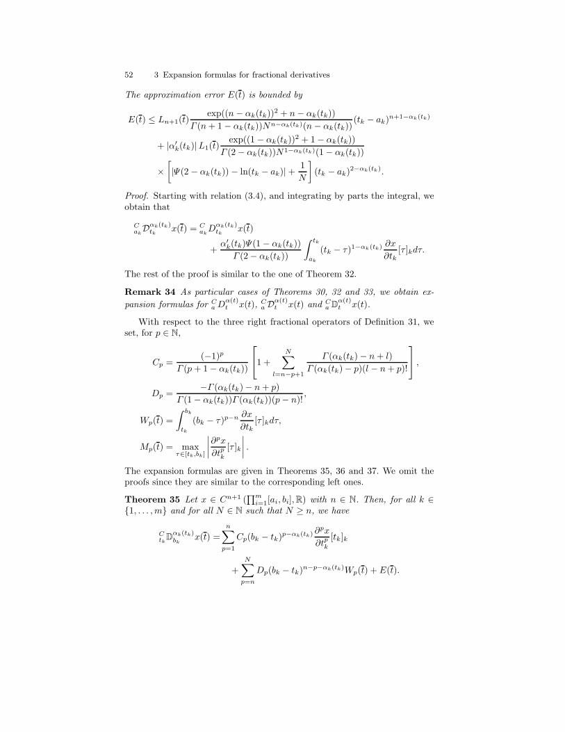
52 3 Expansion formulas for fractional derivatives
The approximation error E(t) is bounded by
E(t) ≤ Ln+1(t)exp((n− αk(tk))
2 + n− αk(tk))
Γ (n+ 1− αk(tk))Nn−αk(tk)(n− αk(tk))(tk − ak)
n+1−αk(tk)
+ |α′k(tk)|L1(t)
exp((1 − αk(tk))2 + 1− αk(tk))
Γ (2− αk(tk))N1−αk(tk)(1− αk(tk))
×[
|Ψ(2 − αk(tk))− ln(tk − ak)|+1
N
]
(tk − ak)2−αk(tk).
Proof. Starting with relation (3.4), and integrating by parts the integral, weobtain that
CakDαk(tk)
tk x(t) = CakD
αk(tk)tk x(t)
+α′k(tk)Ψ(1 − αk(tk))
Γ (2− αk(tk))
∫ tk
ak
(tk − τ)1−αk(tk)∂x
∂tk[τ ]kdτ.
The rest of the proof is similar to the one of Theorem 32.
Remark 34 As particular cases of Theorems 30, 32 and 33, we obtain ex-
pansion formulas for CaD
α(t)t x(t), C
a Dα(t)t x(t) and C
a Dα(t)t x(t).
With respect to the three right fractional operators of Definition 31, weset, for p ∈ N,
Cp =(−1)p
Γ (p+ 1− αk(tk))
1 +
N∑
l=n−p+1
Γ (αk(tk)− n+ l)
Γ (αk(tk)− p)(l − n+ p)!
,
Dp =−Γ (αk(tk)− n+ p)
Γ (1− αk(tk))Γ (αk(tk))(p− n)!,
Wp(t) =
∫ bk
tk
(bk − τ)p−n ∂x
∂tk[τ ]kdτ,
Mp(t) = maxτ∈[tk,bk]
∣
∣
∣
∣
∂px
∂tpk[τ ]k
∣
∣
∣
∣
.
The expansion formulas are given in Theorems 35, 36 and 37. We omit theproofs since they are similar to the corresponding left ones.
Theorem 35 Let x ∈ Cn+1 (∏m
i=1[ai, bi],R) with n ∈ N. Then, for all k ∈1, . . . ,m and for all N ∈ N such that N ≥ n, we have
CtkD
αk(tk)bk
x(t) =
n∑
p=1
Cp(bk − tk)p−αk(tk)
∂px
∂tpk[tk]k
+N∑
p=n
Dp(bk − tk)n−p−αk(tk)Wp(t) + E(t).

3.2 Numerical approximations 53
The approximation error E(t) is bounded by
E(t) ≤Mn+1(t)exp((n− αk(tk))
2 + n− αk(tk))
Γ (n+ 1− αk(tk))Nn−αk(tk)(n− αk(tk))(bk − tk)
n+1−αk(tk).
Theorem 36 Let x ∈ Cn+1 (∏m
i=1[ai, bi],R) with n ∈ N. Then, for all k ∈1, . . . ,m and for all N ∈ N such that N ≥ n, we have
CtkD
αk(tk)bk
x(t) =
n∑
p=1
Cp(bk − tk)p−αk(tk)
∂px
∂tpk[tk]k
+
N∑
p=n
Dp(bk − tk)n−p−αk(tk)Wp(t) +
α′k(tk)(bk − tk)
1−αk(tk)
Γ (2− αk(tk))
×[
(
1
1− αk(tk)− ln(bk − tk)
) N∑
p=0
(
1−αk(tk)p
) (−1)p
(bk − tk)pWn+p(t)
+N∑
p=0
(
1−αk(tk)p
)
(−1)pN∑
r=1
1
r(bk − tk)p+rWn+p+r(t)
]
+ E(t).
The approximation error E(t) is bounded by
E(t) ≤Mn+1(t)exp((n− αk(tk))
2 + n− αk(tk))
Γ (n+ 1− αk(tk))Nn−αk(tk)(n− αk(tk))(bk − tk)
n+1−αk(tk)
+ |α′k(tk)|M1(t)
exp((1 − αk(tk))2 + 1− αk(tk))
Γ (2− αk(tk))N1−αk(tk)(1 − αk(tk))
×[∣
∣
∣
∣
1
1− αk(tk)− ln(bk − tk)
∣
∣
∣
∣
+1
N
]
(bk − tk)2−αk(tk).
Theorem 37 Let x ∈ Cn+1 (∏m
i=1[ai, bi],R) with n ∈ N. Then, for all k ∈1, . . . ,m and for all N ∈ N such that N ≥ n, we have
CtkD
αk(tk)bk
x(t) =
n∑
p=1
Cp(bk − tk)p−αk(tk)
∂px
∂tpk[tk]k
+
N∑
p=n
Dp(bk − tk)n−p−αk(tk)Wp(t) +
α′k(tk)(bk − tk)
1−αk(tk)
Γ (2− αk(tk))
×[
(Ψ(2− αk(tk))− ln(bk − tk))
N∑
p=0
(
1−αk(tk)p
) (−1)p
(bk − tk)pWn+p(t)
+
N∑
p=0
(
1−αk(tk)p
)
(−1)pN∑
r=1
1
r(bk − tk)p+rWn+p+r(t)
]
+ E(t).
The approximation error E(t) is bounded by

54 3 Expansion formulas for fractional derivatives
E(t) ≤Mn+1(t)exp((n− αk(tk))
2 + n− αk(tk))
Γ (n+ 1− αk(tk))Nn−αk(tk)(n− αk(tk))(bk − tk)
n+1−αk(tk)
+ |α′k(tk)|M1(t)
exp((1 − αk(tk))2 + 1− αk(tk))
Γ (2− αk(tk))N1−αk(tk)(1 − αk(tk))
×[
|Ψ(2 − αk(tk))− ln(bk − tk)|+1
N
]
(bk − tk)2−αk(tk).
3.3 Example
To test the accuracy of the proposed method, we compare the fractionalderivative of a concrete given function with some numerical approximationsof it. For t ∈ [0, 1], let x(t) = t2 be the test function. For the order of thefractional derivatives we consider two cases:
α(t) =50t+ 49
100and β(t) =
t+ 5
10.
We consider the approximations given in Theorems 30, 32 and 33, with a fixedn = 1 and N ∈ 2, 4, 6. The error of approximating f(t) by f(t) is measuredby |f(t)− f(t)|. See Figures 3.2–3.7.
(a) C0 D
α(t)t x(t) (b) Error
Fig. 3.2. Type III left Caputo derivative of order α(t) for the example of Sec-tion 3.3—analytic versus numerical approximations obtained from Theorem 30.
3.4 Applications
In this section we apply the proposed technique to some concrete fractionaldifferential equations of physical relevance.

3.4 Applications 55
(a) C0 D
α(t)t x(t) (b) Error
Fig. 3.3. Type I left Caputo derivative of order α(t) for the example of Section 3.3—analytic versus numerical approximations obtained from Theorem 32.
(a) C0 D
α(t)t x(t) (b) Error
Fig. 3.4. Type II left Caputo derivative of order α(t) for the example of Section 3.3—analytic versus numerical approximations obtained from Theorem 33.
3.4.1 A time-fractional diffusion equation
We extend the one-dimensional time-fractional diffusion equation (Lin and Xu,2007) to the variable-order case. Consider u = u(x, t) with domain [0, 1]2. Thepartial fractional differential equation of order α(t) is the following:
C0 D
α(t)t u(x, t)− ∂2u
∂x2(x, t) = f(x, t) for x ∈ [0, 1], t ∈ [0, 1], (3.8)
subject to the boundary conditions
u(x, 0) = g(x), for x ∈ (0, 1), (3.9)

56 3 Expansion formulas for fractional derivatives
(a) C0 D
β(t)t x(t) (b) Error
Fig. 3.5. Type III left Caputo derivative of order β(t) for the example of Sec-tion 3.3—analytic versus numerical approximations obtained from Theorem 30.
(a) C0 D
β(t)t x(t) (b) Error
Fig. 3.6. Type I left Caputo derivative of order β(t) for the example of Section 3.3—analytic versus numerical approximations obtained from Theorem 32.
andu(0, t) = u(1, t) = 0, for t ∈ [0, 1]. (3.10)
We mention that when α(t) ≡ 1, one obtains the classical diffusion equation,and when α(t) ≡ 0 one gets the classical Helmholtz elliptic equation. UsingLemma 27, it is easy to check that
u(x, t) = t2 sin(2πx)
is a solution to (3.8)–(3.10) with

3.4 Applications 57
(a) C0 D
β(t)t x(t) (b) Error
Fig. 3.7. Type II left Caputo derivative of order β(t) for the example of Section 3.3—analytic versus numerical approximations obtained from Theorem 33.
f(x, t) =
(
2
Γ (3− α(t))t2−α(t) + 4π2t2
)
sin(2πx)
andg(x) = 0
(compare with Example 1 in (Lin and Xu, 2007)). The numerical procedure is
the following: replace C0 D
α(t)t u with the approximation given in Theorem 30,
taking n = 1 and an arbitrary N ≥ 1, that is,
C0 D
α(t)t u(x, t) ≈ At1−α(t) ∂u
∂t(x, t) +
N∑
p=1
Bpt1−p−α(t)Vp(x, t)
with
A =1
Γ (2− α(t))
[
1 +
N∑
l=1
Γ (α(t)− 1 + l)
Γ (α(t)− 1)l!
]
,
Bp =Γ (α(t)− 1 + p)
Γ (1− α(t))Γ (α(t))(p− 1)!,
Vp(x, t) =
∫ t
0
τp−1 ∂u
∂t(x, τ)dτ.
Then, the initial fractional problem (3.8)–(3.10) is approximated by the fol-lowing system of second-order partial differential equations:
At1−α(t) ∂u
∂t(x, t) +
N∑
p=1
Bpt1−p−α(t)Vp(x, t)−
∂2u
∂x2(x, t) = f(x, t)

58 3 Expansion formulas for fractional derivatives
and∂Vp∂t
(x, t) = tp−1 ∂u
∂t(x, t), p = 1, . . . , N,
for x ∈ [0, 1] and for t ∈ [0, 1], subject to the boundary conditions
u(x, 0) = 0, for x ∈ (0, 1),
u(0, t) = u(1, t) = 0, for t ∈ [0, 1],
andVp(x, 0) = 0, for x ∈ [0, 1], p = 1, . . . , N.
3.4.2 A fractional partial differential equation in fluid mechanics
We now apply our approximation techniques to the following one-dimensionallinear inhomogeneous fractional Burgers’ equation of variable-order (see (Odibat and Momani,2009, Example 5.2)):
C0 D
α(t)t u(x, t) +
∂u
∂x(x, t)− ∂2u
∂x2(x, t) =
2t2−α(t)
Γ (3− α(t))+ 2x− 2, (3.11)
for x ∈ [0, 1] and t ∈ [0, 1], subject to the boundary condition
u(x, 0) = x2, for x ∈ (0, 1). (3.12)
Here,
F (x, t) =2t2−α(t)
Γ (3− α(t))+ 2x− 2
is the external force field. Burgers’ equation is used to model gas dynamics,traffic flow, turbulence, fluid mechanics, etc. The exact solution is
u(x, t) = x2 + t2.
The fractional problem (3.11)–(3.12) can be approximated by
At1−α(t) ∂u
∂t(x, t) +
N∑
p=1
Bpt1−p−α(t)Vp(x, t) +
∂u
∂x(x, t)− ∂2u
∂x2(x, t)
=2t2−α(t)
Γ (3− α(t))+ 2x− 2
with A, Bp and Vp, p ∈ 1, . . . , N, as in Section 3.4.1. The approximationerror can be decreased as much as desired by increasing the value of N .

References 59
References
Caputo M (1967) Linear model of dissipation whose Q is almost frequencyindependent–II. Geophys. J. R. Astr. Soc. 13:529–539
Chechkin AV, Gorenflo R, Sokolov IM (2005) Fractional diffusion in inhomo-geneous media. J. Phys. A: Math. Theor. 38(42):L679–L684
Dalir M, Bashour M (2010) Applications of fractional calculus. Appl. Math.Sci. 4(21–24):1021–1032
Diethelm K (2004) The Analysis of Fractional Differential Equations. LectureNotes in Mathematics 2004, Springer, Berlin
Dzrbasjan MM, Nersesjan AB (1968) Fractional derivatives and the Cauchyproblem for differential equations of fractional order. Izv. Akad. Nauk Ar-mjan. SSR Ser. Mat. 3(1):3–29
Lin Y, Xu C (2007) Finite difference/spectral approximations for the time-fractional diffusion equation. J. Comput. Phys. 225(2):1533–1552
Machado JAT, Silva MF, Barbosa RS, Jesus IS, Reis CM, Marcos MG, Gal-hano AF (2010) Some applications of fractional calculus in engineering.Math. Probl. Eng. 2010:Art. ID 639801, 34 pp
Murio DA, Mejıa CE (2008) Generalized time fractional IHCP with Caputofractional derivatives. J. Phys. Conf. Ser. 135:Art. ID 012074, 8 pp
Odibat Z, Momani S (2009) The variational iteration method: an efficientscheme for handling fractional partial differential equations in fluid me-chanics. Comput. Math. Appl. 58(11-12):2199–2208
Rabotnov YN (1969) Creep Problems in Structural Members. North-HollandSeries in Applied Mathematics and Mechanics, Amsterdam/London
Samko SG, Kilbas AA, Marichev OI (1993) Fractional Integrals and Deriva-tives. translated from the 1987 Russian original, Gordon and Breach, Yver-don
Samko SG, Ross B (1993) Integration and differentiation to a variable frac-tional order. Integral Transform. Spec. Funct. 1(4):277–300
Santamaria F, Wils S, Schutter E, Augustine GJ (2006) Anomalous diffusionin Purkinje cell dendrites caused by spines. Neuron. 52:635–648
Singh K, Saxena R, Kumar S (2013) Caputo-based fractional derivative infractional Fourier transform domain. IEEE Journal on Emerging and Se-lected Topics in Circuits and Systems 3:330–337
Sun HG, Chen W, Chen YQ (2009) Variable order fractional differential op-erators in anomalous diffusion modeling. Physica A. 388(21):4586–4592
Sweilam NH, AL-Mrawm HM (2011) On the numerical solutions of the vari-able order fractional heat equation. Studies in Nonlinear Sciences 2:31–36
Tavares D, Almeida R, Torres DFM (2016) Caputo derivatives of fractionalvariable order: numerical approximations. Commun. Nonlinear Sci. Numer.Simul. 35:69–87 arXiv:1511.02017
Yajima T, Yamasaki K (2012) Geometry of surfaces with Caputo fractionalderivatives and applications to incompressible two-dimensional flows. J.Phys. A 45(6):065201, 15 pp


4
The fractional calculus of variations
In this chapter, we consider general fractional problems of the calculus ofvariations, where the Lagrangian depends on a combined Caputo fractional
derivative of variable fractional order CDα(·,·),β(·,·)γ given as a combination
of the left and the right Caputo fractional derivatives of orders, respectively,α(·, ·) and β(·, ·). More specifically, here we study some problems of the cal-culus of variations with integrands depending on the independent variable t,
an arbitrary function x and a fractional derivative CDα(·,·),β(·,·)γ x defined by
CDα(·,·),β(·,·)γ x(t) = γ1
CaD
α(·,·)t x(t) + γ2
Ct D
β(·,·)b x(t),
where γ = (γ1, γ2) ∈ [0, 1]2, with γ1 and γ2 not both zero.Starting from the fundamental variational problem, we investigate different
types of variational problems: problems with time delay or with higher-orderderivatives, isoperimetric problems, problems with holonomic constraints andproblems of Herglotz and those depending on combined Caputo fractionalderivatives of variable-order. Our variational problems are known as free-timeproblems because, in general, we impose a boundary condition at the initialtime t = a, but we consider the endpoint b of the integral and the terminalstate x(b) to be free (variable). The main results provide necessary optimalityconditions of Euler–Lagrange type, described by fractional differential equa-tions of variable-order, and different transversality optimality conditions.
Our main contributions are to consider the Lagrangian containing a frac-tional operator where the order is not a constant, and may depend on time.Moreover, we do not only assume that x(b) is free, but the endpoint b is alsofree.
In Section 4.1, we introduce the combined Caputo fractional derivativeof variable-order and provide the necessary concepts and results needed inthe sequel (Section 4.1.1). We deduce two formulas of integration by partsthat involve the combined Caputo fractional derivative of higher order (Sec-tion 4.1.2).

62 4 The fractional calculus of variations
The fractional variational problems under our consideration are formulated
in terms of the fractional derivative CDα(·,·),β(·,·)γ . We discuss the fundamen-
tal concepts of a variational calculus such as the Euler–Lagrange equationsand transversality conditions (Section 4.2), variational problems involvinghigher-order derivatives (Section 4.3), variational problems with time delay(Section 4.4), isoperimetric problems (Section 4.5), problems with holonomicconstraints (Section 4.6) and the last Section 4.7 investigates fractional vari-ational Herglotz problems.
Some illustrative examples are presented for all considered variationalproblems.
The results of this chapter first appeared in (Tavares, Almeida and Torres,2015, 2017, 2018a,b).
4.1 Introduction
In this section, we recall the fundamental definition of the combined Caputofractional derivative presented in Section 1.3.3 (see Definition 15), and gen-eralize it for fractional variable-order. In the end, we prove an integrationby parts formula, involving the higher-order Caputo fractional derivative ofvariable-order.
4.1.1 Combined operators of variable-order
Motivated by the combined fractional Caputo derivative, we propose the fol-lowing definitions about combined variable-order fractional calculus.
Let α, β : [a, b]2 → (0, 1) be two functions and γ = (γ1, γ2) ∈ [0, 1]2 avector, with γ1 and γ2 not both zero.
Definition 32 The combined Riemann–Liouville fractional derivative of variable-
order, denoted by Dα(·,·),β(·,·)γ , is defined by
Dα(·,·),β(·,·)γ = γ1 aD
α(·,·)t + γ2 tD
β(·,·)b ,
acting on x ∈ C([a, b];R) in the following way:
Dα(·,·),β(·,·)γ x(t) = γ1 aD
α(·,·)t x(t) + γ2 tD
β(·,·)b x(t).
Definition 33 The combined Caputo fractional derivative operator of variable-
order, denoted by CDα(·,·),β(·,·)γ , is defined by
CDα(·,·),β(·,·)γ = γ1
CaD
α(·,·)t + γ2
Ct D
β(·,·)b ,
acting on x ∈ C1([a, b];R) in the following way:
CDα(·,·),β(·,·)γ x(t) = γ1
CaD
α(·,·)t x(t) + γ2
Ct D
β(·,·)b x(t).

4.1 Introduction 63
In the sequel, we need the auxiliary notation of the dual fractional deriva-tive, defined by
Dβ(·,·),α(·,·)γ = γ2 aD
β(·,·)t + γ1 tD
α(·,·)T , (4.1)
where γ = (γ2, γ1) and T ∈ (a, b].To generalize the concept of the combined fractional derivative to higher
orders, we need to review some definitions of higher-order operators.Let n ∈ N and x : [a, b] → R be a function of class Cn. The fractional
order is a continuous function of two variables, αn : [a, b]2 → (n− 1, n).
Definition 34 The left and right Riemann–Liouville fractional integrals oforder αn(·, ·) are defined respectively by
aIαn(·,·)t x(t) =
∫ t
a
1
Γ (αn(t, τ))(t− τ)αn(t,τ)−1x(τ)dτ
and
tIαn(·,·)b x(t) =
∫ b
t
1
Γ (αn(τ, t))(τ − t)αn(τ,t)−1x(τ)dτ.
With this definition of Riemann–Liouville fractional integrals of variable-order, and considering n = 1, in Appendix A.1 we implemented two func-tions leftFI(x,alpha,a) and rightFI(x,alpha,b) that approximate, re-
spectively, the Riemann–Liouville fractional integrals aIαn(·,·)t x and tI
αn(·,·)b x,
using the open source software package Chebfun (Trefethen, 2013). Withthese two functions we present also, in Appendix A.1, an illustrative ex-ample where we determine computational approximations to the fractionalintegrals for a specific power function of the form x(t) = tγ (see Example 4.4in Appendix A.1). For this numerical computations, we have used MATLAB
(Linge and Langtangen, 2016).
Definition 35 The left and right Riemann–Liouville fractional derivatives oforder αn(·, ·) are defined by
aDαn(·,·)t x(t) =
dn
dtn
∫ t
a
1
Γ (n− αn(t, τ))(t− τ)n−1−αn(t,τ)x(τ)dτ
and
tDαn(·,·)b x(t) = (−1)n
dn
dtn
∫ b
t
1
Γ (n− αn(τ, t))(τ − t)n−1−αn(τ,t)x(τ)dτ,
respectively.
Definition 36 The left and right Caputo fractional derivatives of orderαn(·, ·) are defined by

64 4 The fractional calculus of variations
CaD
αn(·,·)t x(t) =
∫ t
a
1
Γ (n− αn(t, τ))(t− τ)n−1−αn(t,τ)x(n)(τ)dτ (4.2)
and
Ct D
αn(·,·)b x(t) = (−1)n
∫ b
t
1
Γ (n− αn(τ, t))(τ − t)n−1−αn(τ,t)x(n)(τ)dτ, (4.3)
respectively.
Remark 38 Definitions 35 and 36, for the particular case of order between0 and 1, can be found in (Malinowska, Odzijewicz and Torres, 2015). Theyseem to be new for the higher-order case.
Considering Definition 36, in Appendix A.2 we implement two new func-tions leftCaputo(x,alpha,a,n) and rightCaputo(x,alpha,b,n) that ap-
proximate the higher-order Caputo fractional derivatives CaD
αn(·,·)t x and C
t Dαn(·,·)b x,
respectively. With these two functions, we present, also in Appendix A.2, anillustrative example where we study approximations to the Caputo fractionalderivatives for a specific power function of the form x(t) = tγ (see Example 4.5in Appendix A.2).
Remark 39 From Definition 34, it follows that
aDαn(·,·)t x(t) =
dn
dtnaI
n−αn(·,·)t x(t), tD
αn(·,·)b x(t) = (−1)n
dn
dtntI
n−αn(·,·)b x(t)
and
CaD
αn(·,·)t x(t) = aI
n−αn(·,·)t
dn
dtnx(t), C
t Dαn(·,·)b x(t) = (−1)n tI
n−αn(·,·)b
dn
dtnx(t).
In Lemma 40, we obtain higher-order Caputo fractional derivatives of apower function. For that, we assume that the fractional order depends onlyon the first variable: αn(t, τ) := αn(t), where αn : [a, b] → (n− 1, n) is a givenfunction.
Lemma 40 Let x(t) = (t− a)γ with γ > n− 1. Then,
CaD
αn(t)t x(t) =
Γ (γ + 1)
Γ (γ − αn(t) + 1)(t− a)γ−αn(t).
Proof. As x(t) = (t− a)γ , if we differentiate it n times, we obtain
x(n)(t) =Γ (γ + 1)
Γ (γ − n+ 1)(t− a)γ−n.
Using Definition 36 of the left Caputo fractional derivative, we get
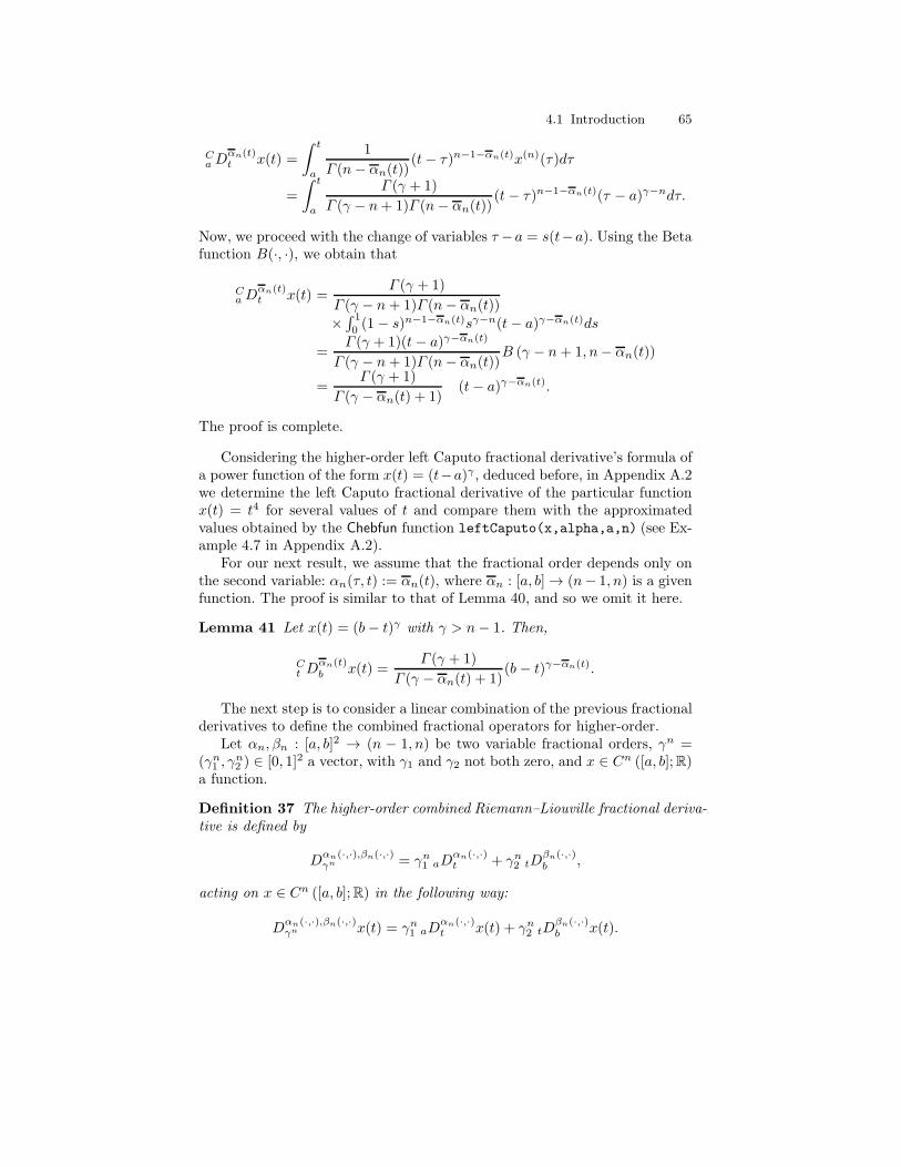
4.1 Introduction 65
CaD
αn(t)t x(t) =
∫ t
a
1
Γ (n− αn(t))(t− τ)n−1−αn(t)x(n)(τ)dτ
=
∫ t
a
Γ (γ + 1)
Γ (γ − n+ 1)Γ (n− αn(t))(t− τ)n−1−αn(t)(τ − a)γ−ndτ.
Now, we proceed with the change of variables τ −a = s(t−a). Using the Betafunction B(·, ·), we obtain that
CaD
αn(t)t x(t) =
Γ (γ + 1)
Γ (γ − n+ 1)Γ (n− αn(t))
×∫ 1
0(1− s)n−1−αn(t)sγ−n(t− a)γ−αn(t)ds
=Γ (γ + 1)(t− a)γ−αn(t)
Γ (γ − n+ 1)Γ (n− αn(t))B (γ − n+ 1, n− αn(t))
=Γ (γ + 1)
Γ (γ − αn(t) + 1)(t− a)γ−αn(t).
The proof is complete.
Considering the higher-order left Caputo fractional derivative’s formula ofa power function of the form x(t) = (t−a)γ , deduced before, in Appendix A.2we determine the left Caputo fractional derivative of the particular functionx(t) = t4 for several values of t and compare them with the approximatedvalues obtained by the Chebfun function leftCaputo(x,alpha,a,n) (see Ex-ample 4.7 in Appendix A.2).
For our next result, we assume that the fractional order depends only onthe second variable: αn(τ, t) := αn(t), where αn : [a, b] → (n− 1, n) is a givenfunction. The proof is similar to that of Lemma 40, and so we omit it here.
Lemma 41 Let x(t) = (b− t)γ with γ > n− 1. Then,
Ct D
αn(t)b x(t) =
Γ (γ + 1)
Γ (γ − αn(t) + 1)(b − t)γ−αn(t).
The next step is to consider a linear combination of the previous fractionalderivatives to define the combined fractional operators for higher-order.
Let αn, βn : [a, b]2 → (n − 1, n) be two variable fractional orders, γn =(γn1 , γ
n2 ) ∈ [0, 1]2 a vector, with γ1 and γ2 not both zero, and x ∈ Cn ([a, b];R)
a function.
Definition 37 The higher-order combined Riemann–Liouville fractional deriva-tive is defined by
Dαn(·,·),βn(·,·)γn = γn1 aD
αn(·,·)t + γn2 tD
βn(·,·)b ,
acting on x ∈ Cn ([a, b];R) in the following way:
Dαn(·,·),βn(·,·)γn x(t) = γn1 aD
αn(·,·)t x(t) + γn2 tD
βn(·,·)b x(t).

66 4 The fractional calculus of variations
In our work, we use both Riemann–Liouville and Caputo derivatives defi-nitions. The emphasis is, however, in Caputo fractional derivatives.
Definition 38 The higher-order combined Caputo fractional derivative of xat t is defined by
CDαn(·,·),βn(·,·)γn x(t) = γn1
CaD
αn(·,·)t x(t) + γn2
Ct D
βn(·,·)b x(t).
Similarly, in the sequel of this work, we need the auxiliary notation of thedual fractional derivative:
Dβi(·,·),αi(·,·)γi
= γi2 aDβi(·,·)t + γi1 tD
αi(·,·)T , (4.4)
where γi = (γi2, γi1) and T ∈ (a, b].
Some computational aspects about the combined Caputo fractional deriva-tive of variable-order, are also discussed in Appendix A.3, using the softwarepackage Chebfun. For that, we developed the new function (see Example 4.8in Appendix A.3) combinedCaputo(x,alpha,beta,gamma1,gamma2,a,b,n)
and obtained approximated values for a particular power function.
4.1.2 Generalized fractional integration by parts
When dealing with variational problems, one key property is integration byparts. Formulas of integration by parts have an important role in the proofof Euler–Lagrange conditions. In the following theorem, such formulas areproved for integrals involving higher-order Caputo fractional derivatives ofvariable-order.
Let n ∈ N and x, y ∈ Cn ([a, b];R) be two functions. The fractional orderis a continuous function of two variables, αn : [a, b]2 → (n− 1, n).
Theorem 42 The higher-order Caputo fractional derivatives of variable-order satisfy the integration by parts formulas
∫ b
a
y(t)CaDαn(·,·)t x(t)dt =
∫ b
a
x(t) tDαn(·,·)b y(t)dt
+
[
n−1∑
k=0
(−1)kx(n−1−k)(t)dk
dtktI
n−αn(·,·)b y(t)
]t=b
t=a
and
∫ b
a
y(t)Ct Dαn(·,·)b x(t)dt =
∫ b
a
x(t) aDαn(·,·)t y(t)dt
+
[
n−1∑
k=0
(−1)n+kx(n−1−k)(t)dk
dtkaI
n−αn(·,·)t y(t)
]t=b
t=a
.

4.1 Introduction 67
Proof. Considering the Definition 36 of left Caputo fractional derivatives oforder αn(·, ·), we obtain
∫ b
a
y(t)CaDαn(·,·)t x(t)dt
=
∫ b
a
∫ t
a
y(t)1
Γ (n− αn(t, τ))(t− τ)n−1−αn(t,τ)x(n)(τ)dτdt.
Using Dirichelt’s Formula, we rewrite it as
∫ b
a
∫ b
t
y(τ)(τ − t)n−1−αn(τ,t)
Γ (n− αn(τ, t))x(n)(t)dτdt
=
∫ b
a
x(n)(t)
∫ b
t
(τ − t)n−1−αn(τ,t)
Γ (n− αn(τ, t))y(τ)dτdt =
∫ b
a
x(n)(t) tIn−αn(·,·)b y(t)dt.
(4.5)
Using the (usual) integrating by parts formula, we get that (4.5) is equal to
−∫ b
a
x(n−1)(t)d
dttI
n−αn(·,·)b y(t)dt+
[
x(n−1)(t)tIn−αn(·,·)b y(t)
]t=b
t=a.
Integrating by parts again, we obtain
∫ b
a
x(n−2)(t)d2
dt2tI
n−αn(·,·)b y(t)dt
+
[
x(n−1)(t) tIn−αn(·,·)b y(t)− x(n−2)(t)
d
dttI
n−αn(·,·)b y(t)
]t=b
t=a
.
If we repeat this process n− 2 times more, we get
∫ b
a
x(t)(−1)ndn
dtntI
n−αn(·,·)b y(t)dt
+
[
n−1∑
k=0
(−1)kx(n−1−k)(t)dk
dtktI
n−αn(·,·)b y(t)
]t=b
t=a
=
∫ b
a
x(t)tDαn(·,·)b y(t)dt+
[
n−1∑
k=0
(−1)kx(n−1−k)(t)dk
dtktI
n−αn(·,·)b y(t)
]t=b
t=a
.
The second relation of the theorem for the right Caputo fractional deriva-tive of order αn(·, ·), follows directly from the first by Caputo–Torres duality(Caputo and Torres, 2015).
Remark 43 If we consider in Theorem 42 the particular case when n = 1,then the fractional integration by parts formulas take the well-known formspresented in Theorem 13.
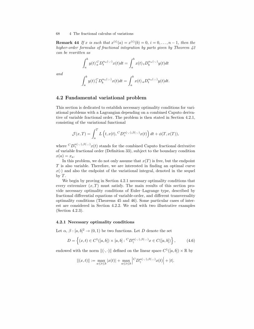
68 4 The fractional calculus of variations
Remark 44 If x is such that x(i)(a) = x(i)(b) = 0, i = 0, . . . , n− 1, then thehigher-order formulas of fractional integration by parts given by Theorem 42can be rewritten as
∫ b
a
y(t)CaDαn(·,·)t x(t)dt =
∫ b
a
x(t) tDαn(·,·)b y(t)dt
and∫ b
a
y(t)Ct Dαn(·,·)b x(t)dt =
∫ b
a
x(t) aDαn(·,·)t y(t)dt.
4.2 Fundamental variational problem
This section is dedicated to establish necessary optimality conditions for vari-ational problems with a Lagrangian depending on a combined Caputo deriva-tive of variable fractional order. The problem is then stated in Section 4.2.1,consisting of the variational functional
J (x, T ) =
∫ T
a
L(
t, x(t),CDα(·,·),β(·,·)γ x(t)
)
dt+ φ(T, x(T )),
where CDα(·,·),β(·,·)γ x(t) stands for the combined Caputo fractional derivative
of variable fractional order (Definition 33), subject to the boundary conditionx(a) = xa.
In this problem, we do not only assume that x(T ) is free, but the endpointT is also variable. Therefore, we are interested in finding an optimal curvex(·) and also the endpoint of the variational integral, denoted in the sequelby T .
We begin by proving in Section 4.2.1 necessary optimality conditions thatevery extremizer (x, T ) must satisfy. The main results of this section pro-vide necessary optimality conditions of Euler–Lagrange type, described byfractional differential equations of variable-order, and different transversalityoptimality conditions (Theorems 45 and 46). Some particular cases of inter-est are considered in Section 4.2.2. We end with two illustrative examples(Section 4.2.3).
4.2.1 Necessary optimality conditions
Let α, β : [a, b]2 → (0, 1) be two functions. Let D denote the set
D =
(x, t) ∈ C1([a, b])× [a, b] : CDα(·,·),β(·,·)γ x ∈ C([a, b])
, (4.6)
endowed with the norm ‖(·, ·)‖ defined on the linear space C1([a, b])× R by
‖(x, t)‖ := maxa≤t≤b
|x(t)|+ maxa≤t≤b
∣
∣
∣
CDα(·,·),β(·,·)γ x(t)
∣
∣
∣+ |t|.

4.2 Fundamental variational problem 69
Definition 39 We say that (x⋆, T ⋆) ∈ D is a local minimizer to the func-tional J : D → R if there exists some ǫ > 0 such that
∀(x, T ) ∈ D : ‖(x⋆, T ⋆)− (x, T )‖ < ǫ⇒ J(x⋆, T ⋆) ≤ J(x, T ).
Along the work, we denote by ∂iz, i ∈ 1, 2, 3, the partial derivative of afunction z : R3 → R with respect to its ith argument, and by L a differentiableLagrangian L : [a, b]× R
2 → R.Consider the following problem of the calculus of variations:
Problem 1 Find the local minimizers of the functional J : D → R, with
J (x, T ) =
∫ T
a
L(
t, x(t),CDα(·,·),β(·,·)γ x(t)
)
dt+ φ(T, x(T )), (4.7)
over all (x, T ) ∈ D satisfying the boundary condition x(a) = xa, for a fixedxa ∈ R. The terminal time T and terminal state x(T ) are free.The terminal cost function φ : [a, b]× R → R is at least of class C1.
For simplicity of notation, we introduce the operator [·]α,βγ defined by
[x]α,βγ (t) =(
t, x(t),CDα(·,·),β(·,·)γ x(t)
)
. (4.8)
With the new notation, one can write (4.7) simply as
J (x, T ) =
∫ T
a
L[x]α,βγ (t)dt+ φ(T, x(T )).
The next theorem gives fractional necessary optimality conditions to Prob-lem 1.
Theorem 45 Suppose that (x, T ) is a local minimizer to the functional (4.7)on D. Then, (x, T ) satisfies the fractional Euler–Lagrange equations
∂2L[x]α,βγ (t) +D
β(·,·),α(·,·)γ ∂3L[x]
α,βγ (t) = 0, (4.9)
on the interval [a, T ], and
γ2
(
aDβ(·,·)t ∂3L[x]
α,βγ (t)− TD
β(·,·)t ∂3L[x]
α,βγ (t)
)
= 0, (4.10)
on the interval [T, b]. Moreover, (x, T ) satisfies the transversality conditions
L[x]α,βγ (T ) + ∂1φ(T, x(T )) + ∂2φ(T, x(T ))x′(T ) = 0,
[
γ1 tI1−α(·,·)T ∂3L[x]
α,βγ (t)− γ2 T I
1−β(·,·)t ∂3L[x]
α,βγ (t)
]
t=T+ ∂2φ(T, x(T )) = 0,
γ2
[
T I1−β(·,·)t ∂3L[x]
α,βγ (t)− aI
1−β(·,·)t ∂3L[x]
α,βγ (t)
]
t=b= 0.
(4.11)
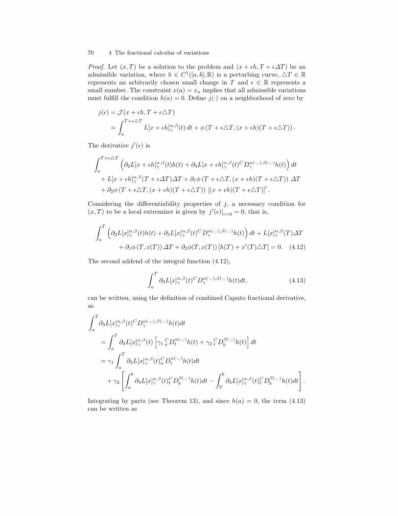
70 4 The fractional calculus of variations
Proof. Let (x, T ) be a solution to the problem and (x+ ǫh, T + ǫ∆T ) be anadmissible variation, where h ∈ C1([a, b];R) is a perturbing curve, T ∈ R
represents an arbitrarily chosen small change in T and ǫ ∈ R represents asmall number. The constraint x(a) = xa implies that all admissible variationsmust fulfill the condition h(a) = 0. Define j(·) on a neighborhood of zero by
j(ǫ) = J (x+ ǫh, T + ǫT )
=
∫ T+ǫT
a
L[x+ ǫh]α,βγ (t) dt+ φ (T + ǫT, (x+ ǫh)(T + ǫT )) .
The derivative j′(ǫ) is
∫ T+ǫT
a
(
∂2L[x+ ǫh]α,βγ (t)h(t) + ∂3L[x+ ǫh]α,βγ (t)CDα(·,·),β(·,·)γ h(t)
)
dt
+ L[x+ ǫh]α,βγ (T + ǫ∆T )∆T + ∂1φ (T + ǫT, (x+ ǫh)(T + ǫT )) ∆T+ ∂2φ (T + ǫT, (x+ ǫh)(T + ǫT )) [(x+ ǫh)(T + ǫT )]′ .
Considering the differentiability properties of j, a necessary condition for(x, T ) to be a local extremizer is given by j′(ǫ)|ǫ=0 = 0, that is,
∫ T
a
(
∂2L[x]α,βγ (t)h(t) + ∂3L[x]
α,βγ (t)CDα(·,·),β(·,·)
γ h(t))
dt+ L[x]α,βγ (T )∆T
+ ∂1φ (T, x(T ))∆T + ∂2φ(T, x(T )) [h(T ) + x′(T )T ] = 0. (4.12)
The second addend of the integral function (4.12),
∫ T
a
∂3L[x]α,βγ (t)CDα(·,·),β(·,·)
γ h(t)dt, (4.13)
can be written, using the definition of combined Caputo fractional derivative,as
∫ T
a
∂3L[x]α,βγ (t)CDα(·,·),β(·,·)
γ h(t)dt
=
∫ T
a
∂3L[x]α,βγ (t)
[
γ1CaD
α(·,·)t h(t) + γ2
Ct D
β(·,·)b h(t)
]
dt
= γ1
∫ T
a
∂3L[x]α,βγ (t)Ca D
α(·,·)t h(t)dt
+ γ2
[
∫ b
a
∂3L[x]α,βγ (t)Ct D
β(·,·)b h(t)dt−
∫ b
T
∂3L[x]α,βγ (t)Ct D
β(·,·)b h(t)dt
]
.
Integrating by parts (see Theorem 13), and since h(a) = 0, the term (4.13)can be written as

4.2 Fundamental variational problem 71
γ1
[
∫ T
a
h(t)tDα(·,·)T ∂3L[x]
α,βγ (t)dt +
[
h(t)tI1−α(·,·)T ∂3L[x]
α,βγ (t)
]
t=T
]
+ γ2
[
∫ b
a
h(t)aDβ(·,·)t ∂3L[x]
α,βγ (t)dt−
[
h(t)aI1−β(·,·)t ∂3L[x]
α,βγ (t)
]
t=b
−(
∫ b
T
h(t)TDβ(·,·)t ∂3L[x]
α,βγ (t)dt−
[
h(t)T I1−β(·,·)t ∂3L[x]
α,βγ (t)
]
t=b
+[
h(t)T I1−β(·,·)t ∂3L[x]
α,βγ (t)
]
t=T
)]
.
Unfolding these integrals, and considering the fractional operator Dβ(·,·),α(·,·)γ
with γ = (γ2, γ1), then (4.13) is equivalent to
∫ T
a
h(t)Dβ(·,·),α(·,·)γ ∂3L[x]
α,βγ (t)dt
+
∫ b
T
γ2h(t)[
aDβ(·,·)t ∂3L[x]
α,βγ (t)− TD
β(·,·)t ∂3L[x]
α,βγ (t)
]
dt
+[
h(t)(
γ1 tI1−α(·,·)T ∂3L[x]
α,βγ (t)− γ2 T I
1−β(·,·)t ∂3L[x]
α,βγ (t)
)]
t=T
+[
h(t)γ2
(
T I1−β(·,·)t ∂3L[x]
α,βγ (t)− aI
1−β(·,·)t ∂3L[x]
α,βγ (t)
)]
t=b.
Substituting these relations into equation (4.12), we obtain
0 =
∫ T
a
h(t)[
∂2L[x]α,βγ (t) +D
β(·,·),α(·,·)γ ∂3L[x]
α,βγ (t)
]
dt
+
∫ b
T
γ2h(t)[
aDβ(·,·)t ∂3L[x]
α,βγ (t)− TD
β(·,·)t ∂3L[x]
α,βγ (t)
]
dt
+ h(T )[
γ1 tI1−α(·,·)T ∂3L[x]
α,βγ (t)− γ2 T I
1−β(·,·)t ∂3L[x]
α,βγ (t)
+ ∂2φ(t, x(t))]
t=T
+∆T[
L[x]α,βγ (t) + ∂1φ(t, x(t)) + ∂2φ(t, x(t))x′(t)]
t=T
+ h(b)[
γ2
(
T I1−β(·,·)t ∂3L[x]
α,βγ (t)− aI
1−β(·,·)t ∂3L[x]
α,βγ (t)
)]
t=b.
(4.14)
As h and T are arbitrary, we can choose T = 0 and h(t) = 0, for allt ∈ [T, b], but h is arbitrary in t ∈ [a, T ). Then, for all t ∈ [a, T ], we obtainthe first necessary condition (4.9):
∂2L[x]α,βγ (t) +D
β(·,·),α(·,·)γ ∂3L[x]
α,βγ (t) = 0.
Analogously, considering T = 0, h(t) = 0, for all t ∈ [a, T ] ∪ b, and harbitrary on (T, b), we obtain the second necessary condition (4.10):

72 4 The fractional calculus of variations
γ2
(
aDβ(·,·)t ∂3L[x]
α,βγ (t)− TD
β(·,·)t ∂3L[x]
α,βγ (t)
)
= 0.
As (x, T ) is a solution to the necessary conditions (4.9) and (4.10), then equa-tion (4.14) takes the form
0 =h(T )[
γ1 tI1−α(·,·)T ∂3L[x]
α,βγ (t)− γ2 T I
1−β(·,·)t ∂3L[x]
α,βγ (t) + ∂2φ(t, x(t))
]
t=T
+∆T[
L[x]α,βγ (t) + ∂1φ(t, x(t)) + ∂2φ(t, x(t))x′(t)]
t=T
+ h(b)[
γ2
(
T I1−β(·,·)t ∂3L[x]
α,βγ (t)− aI
1−β(·,·)t ∂3L[x]
α,βγ (t)
)]
t=b.
(4.15)
Transversality conditions (4.11) are obtained for appropriate choices of vari-ations.
In the next theorem, considering the same Problem 1, we rewrite thetransversality conditions (4.11) in terms of the increment ∆T on time andon the consequent increment ∆xT on x, given by
∆xT = (x+ h) (T +∆T )− x(T ). (4.16)
Theorem 46 Let (x, T ) be a local minimizer to the functional (4.7) on D.Then, the fractional Euler–Lagrange equations (4.9) and (4.10) are satisfiedtogether with the following transversality conditions:
L[x]α,βγ (T ) + ∂1φ(T, x(T ))
+x′(T )[
γ2T I1−β(·,·)t ∂3L[x]
α,βγ (t)− γ1tI
1−α(·,·)T ∂3L[x]
α,βγ (t)
]
t=T= 0,
[
γ1 tI1−α(·,·)T ∂3L[x]
α,βγ (t)− γ2 T I
1−β(·,·)t ∂3L[x]
α,βγ (t)
]
t=T+ ∂2φ(T, x(T )) = 0,
γ2
[
T I1−β(·,·)t ∂3L[x]
α,βγ (t)− aI
1−β(·,·)t ∂3L[x]
α,βγ (t)
]
t=b= 0.
(4.17)
Proof. The Euler–Lagrange equations are deduced following similar argu-ments as the ones presented in Theorem 45. We now focus our attentionon the proof of the transversality conditions. Using Taylor’s expansion up tofirst order for a small ∆T , and restricting the set of variations to those forwhich h′(T ) = 0, we obtain
(x+ h) (T +∆T ) = (x+ h)(T ) + x′(T )∆T +O(∆T )2.
Rearranging the relation (4.16) allows us to express h(T ) in terms of ∆T and∆xT :
h(T ) = ∆xT − x′(T )∆T +O(∆T )2.
Substitution of this expression into (4.15) gives us
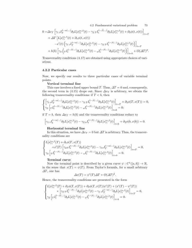
4.2 Fundamental variational problem 73
0 =∆xT
[
γ1 tI1−α(·,·)T ∂3L[x]
α,βγ (t)− γ2 T I
1−β(·,·)t ∂3L[x]
α,βγ (t) + ∂2φ(t, x(t))
]
t=T
+∆T[
L[x]α,βγ (t) + ∂1φ(t, x(t))
−x′(t)(
γ1 tI1−α(·,·)T ∂3L[x]
α,βγ (t)− γ2 T I
1−β(·,·)t ∂3L[x]
α,βγ (t)
)]
t=T
+ h(b)[
γ2
(
T I1−β(·,·)t ∂3L[x]
α,βγ (t)− aI
1−β(·,·)t ∂3L[x]
α,βγ (t)
)]
t=b+O(∆T )2.
Transversality conditions (4.17) are obtained using appropriate choices of vari-ations.
4.2.2 Particular cases
Now, we specify our results to three particular cases of variable terminalpoints.
Vertical terminal lineThis case involves a fixed upper bound T . Thus,∆T = 0 and, consequently,
the second term in (4.15) drops out. Since ∆xT is arbitrary, we obtain thefollowing transversality conditions: if T < b, then
[
γ1 tI1−α(·,·)T ∂3L[x]
α,βγ (t)− γ2 T I
1−β(·,·)t ∂3L[x]
α,βγ (t)
]
t=T+ ∂2φ(T, x(T )) = 0,
γ2
[
T I1−β(·,·)t ∂3L[x]
α,βγ (t)− aI
1−β(·,·)t ∂3L[x]
α,βγ (t)
]
t=b= 0;
if T = b, then ∆xT = h(b) and the transversality conditions reduce to[
γ1 tI1−α(·,·)b ∂3L[x]
α,βγ (t)− γ2 aI
1−β(·,·)t ∂3L[x]
α,βγ (t)
]
t=b+ ∂2φ(b, x(b)) = 0.
Horizontal terminal lineIn this situation, we have∆xT = 0 but∆T is arbitrary. Thus, the transver-
sality conditions are
L[x]α,βγ (T ) + ∂1φ(T, x(T ))
+x′(T )[
γ2T I1−β(·,·)t ∂3L[x]
α,βγ (t)− γ1tI
1−α(·,·)T ∂3L[x]
α,βγ (t)
]
t=T= 0,
γ2
[
T I1−β(·,·)t ∂3L[x]
α,βγ (t)− aI
1−β(·,·)t ∂3L[x]
α,βγ (t)
]
t=b= 0.
Terminal curveNow the terminal point is described by a given curve ψ : C1([a, b]) → R,
in the sense that x(T ) = ψ(T ). From Taylor’s formula, for a small arbitrary∆T , one has
∆x(T ) = ψ′(T )∆T +O(∆T )2.
Hence, the transversality conditions are presented in the form
L[x]α,βγ (T ) + ∂1φ(T, x(T )) + ∂2φ(T, x(T ))ψ′(T ) + (x′(T )− ψ′(T ))
×[
γ2 T I1−β(·,·)t ∂3L[x]
α,βγ (t)− γ1 tI
1−α(·,·)T ∂3L[x]
α,βγ (t)
]
t=T= 0,
γ2
[
T I1−β(·,·)t ∂3L[x]
α,βγ (t)− aI
1−β(·,·)t ∂3L[x]
α,βγ (t)
]
t=b= 0.
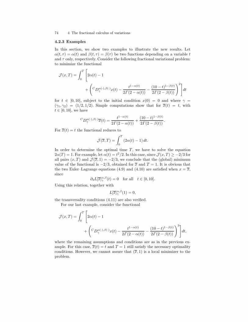
74 4 The fractional calculus of variations
4.2.3 Examples
In this section, we show two examples to illustrate the new results. Letα(t, τ) = α(t) and β(t, τ) = β(τ) be two functions depending on a variable tand τ only, respectively. Consider the following fractional variational problem:to minimize the functional
J (x, T ) =
∫ T
0
[
2α(t)− 1
+
(
CDα(·),β(·)γ x(t)− t1−α(t)
2Γ (2− α(t))− (10− t)1−β(t)
2Γ (2− β(t))
)2]
dt
for t ∈ [0, 10], subject to the initial condition x(0) = 0 and where γ =(γ1, γ2) = (1/2, 1/2). Simple computations show that for x(t) = t, witht ∈ [0, 10], we have
CDα(·),β(·)γ x(t) =
t1−α(t)
2Γ (2− α(t))+
(10− t)1−β(t)
2Γ (2− β(t)).
For x(t) = t the functional reduces to
J (x, T ) =
∫ T
0
(2α(t)− 1)dt.
In order to determine the optimal time T , we have to solve the equation2α(T ) = 1. For example, let α(t) = t2/2. In this case, since J (x, T ) ≥ −2/3 forall pairs (x, T ) and J (x, 1) = −2/3, we conclude that the (global) minimumvalue of the functional is −2/3, obtained for x and T = 1. It is obvious thatthe two Euler–Lagrange equations (4.9) and (4.10) are satisfied when x = x,since
∂3L[x]α,βγ (t) = 0 for all t ∈ [0, 10].
Using this relation, together with
L[x]α,βγ (1) = 0,
the transversality conditions (4.11) are also verified.For our last example, consider the functional
J (x, T ) =
∫ T
0
[
2α(t)− 1
+
(
CDα(·),β(·)γ x(t)− t1−α(t)
2Γ (2− α(t))− (10− t)1−β(t)
2Γ (2− β(t))
)3]
dt,
where the remaining assumptions and conditions are as in the previous ex-ample. For this case, x(t) = t and T = 1 still satisfy the necessary optimalityconditions. However, we cannot assure that (x, 1) is a local minimizer to theproblem.

4.3 Higher-order variational problems 75
4.3 Higher-order variational problems
In this section, we intend to generalize the results obtained in Section 4.2 byconsidering higher-order variational problems with a Lagrangian dependingon a higher-order combined Caputo derivative of variable fractional order,defined by
CDαn(·,·),βn(·,·)γn x(t) = γn1
CaD
αn(·,·)t x(t) + γn2
Ct D
βn(·,·)b x(t),
subject to boundary conditions at the initial time t = a.In Section 4.3.1, we obtain higher-order Euler–Lagrange equations and
transversality conditions for the generalized variational problem with a La-grangian depending on a combined Caputo fractional derivative of variablefractional order (Theorems 47 and 49).
One illustrative example is discussed in Section 4.3.2.
4.3.1 Necessary optimality conditions
Let n ∈ N and x : [a, b] → R be a function of class Cn. The fractional order isa continuous function of two variables, αn : [a, b]2 → (n− 1, n).
Let D denote the linear subspace of Cn([a, b]) × [a, b] such that the frac-
tional derivative of x, CDαi(·,·),βi(·,·)γi x(t), exists and is continuous on the in-
terval [a, b] for all i ∈ 1, . . . , n. We endow D with the norm
‖(x, t)‖ = maxa≤t≤b
|x(t)| + maxa≤t≤b
n∑
i=1
∣
∣
∣
CDαi(·,·),βi(·,·)γi x(t)
∣
∣
∣+ |t|.
Consider the following higher-order problem of the calculus of variations:
Problem 2 Minimize functional J : D → R, where
J (x, T ) =
∫ T
a
L(
t, x(t), CDα1(·,·),β1(·,·)γ1 x(t), . . . , CD
αn(·,·),βn(·,·)γn x(t)
)
dt
+ φ(T, x(T )), (4.18)
over all (x, T ) ∈ D subject to boundary conditions
x(a) = xa, x(i)(a) = xia, ∀i ∈ 1, . . . , n− 1,
for fixed xa, x1a, . . . , x
n−1a ∈ R. Here the terminal time T and terminal state
x(T ) are both free. For all i ∈ 1, . . . , n, αi, βi(
[a, b]2)
⊆ (i − 1, i) and γi =(
γi1, γi2
)
is a vector. The terminal cost function φ : [a, b]× R → R is at leastof class C1.

76 4 The fractional calculus of variations
For simplicity of notation, we introduce the operator [·]α,βγ defined by
[x]α,βγ (t) =(
t, x(t), CDα1(·,·),β1(·,·)γ1 x(t), . . . , CD
αn(·,·),βn(·,·)γn x(t)
)
.
We assume that the Lagrangian L : [a, b]×Rn+1 → R is a function of class C1.
Along the work, we denote by ∂iL, i ∈ 1, . . . , n + 2, the partial derivativeof the Lagrangian L with respect to its ith argument.
Now, we can rewrite functional (4.18) as
J (x, T ) =
∫ T
a
L[x]α,βγ (t)dt+ φ(T, x(T )). (4.19)
In the previous section, we obtained fractional necessary optimality con-ditions that every local minimizer of functional J , with n = 1, must fulfill.Here, we generalize those results to arbitrary values of n, n ∈ N. Necessaryoptimality conditions for Problem 2 are presented next.
Theorem 47 Suppose that (x, T ) gives a minimum to functional (4.19) onD. Then, (x, T ) satisfies the following fractional Euler–Lagrange equations:
∂2L[x]α,βγ (t) +
n∑
i=1
Dβi(·,·),αi(·,·)γi
∂i+2L[x]α,βγ (t) = 0, (4.20)
on the interval [a, T ], and
n∑
i=1
γi2
(
aDβi(·,·)t ∂i+2L[x]
α,βγ (t)− TD
βi(·,·)t ∂i+2L[x]
α,βγ (t)
)
= 0, (4.21)
on the interval [T, b]. Moreover, (x, T ) satisfies the following transversalityconditions:
L[x]α,βγ (T ) + ∂1φ(T, x(T )) + ∂2φ(T, x(T ))x
′(T ) = 0,n∑
i=1
[
γi1(−1)i−1 di−1
dti−1 tIi−αi(·,·)T ∂i+2L[x]
α,βγ (t)
− γi2di−1
dti−1 T Ii−βi(·,·)t ∂i+2L[x]
α,βγ (t)
]
t=T
+ ∂2φ(T, x(T )) = 0,
n∑
i=j+1
[
γi1(−1)i−1−j di−1−j
dti−1−j tIi−αi(·,·)T ∂i+2L[x]
α,βγ (t)
+ γi2(−1)j+1 di−1−j
dti−1−j T Ii−βi(·,·)t ∂i+2L[x]
α,βγ (t)
]
t=T
= 0, ∀j = 1, . . . , n− 1,
n∑
i=j+1
[
γi2(−1)j+1
[
di−1−j
dti−1−j aIi−βi(·,·)t ∂i+2L[x]
α,βγ (t)
− di−1−j
dti−1−j T Ii−βi(·,·)t ∂i+2L[x]
α,βγ (t)
]]
t=b
= 0, ∀j = 0, . . . , n− 1.
(4.22)

4.3 Higher-order variational problems 77
Proof. The proof is an extension of the one used in Theorem 45. Let h ∈Cn([a, b];R) be a perturbing curve and T ∈ R an arbitrarily chosen smallchange in T . For a small number ǫ ∈ R, if (x, T ) is a solution to the problem,we consider an admissible variation of (x, T ) of the form (x+ ǫh, T + ǫ∆T ),and then, by the minimum condition, we have that
J (x, T ) ≤ J (x+ ǫh, T + ǫ∆T ).
The constraints x(i)(a) = x(i)a imply that all admissible variations must fulfill
the conditions h(i)(a) = 0, for all i = 0, . . . , n− 1. We define function j(·) ona neighborhood of zero by
j(ǫ) = J (x+ ǫh, T + ǫT )
=
∫ T+ǫT
a
L[x+ ǫh]α,βγ (t) dt+ φ (T + ǫT, (x+ ǫh)(T + ǫT )) .
The derivative j′(ǫ) is given by the expression
∫ T+ǫT
a
(
∂2L[x+ ǫh]α,βγ (t)h(t) +n∑
i=1
∂i+2L[x+ ǫh]α,βγ (t)CDαi(·,·),βi(·,·)γi h(t)
)
dt
+ L[x+ ǫh]α,βγ (T + ǫ∆T )∆T + ∂1φ (T + ǫT, (x+ ǫh)(T + ǫT )) ∆T+ ∂2φ (T + ǫT, (x+ ǫh)(T + ǫT )) (x + ǫh)′(T + ǫT ).
Hence, by Fermat’s theorem, a necessary condition for (x, T ) to be a localminimizer of j is given by j′(0) = 0, that is,
∫ T
a
(
∂2L[x]α,βγ (t)h(t) +
n∑
i=1
∂i+2L[x]α,βγ (t)CD
αi(·,·),βi(·,·)γi h(t)
)
dt
+ L[x]α,βγ (T )∆T + ∂1φ (T, x(T ))∆T + ∂2φ(T, x(T )) [h(t) + x′(T )T ] = 0.
(4.23)
Considering the second addend of the integral function (4.23), for i = 1, weget
∫ T
a
∂3L[x]α,βγ (t)CD
α1(·,·),β1(·,·)γ1 h(t)dt
=
∫ T
a
∂3L[x]α,βγ (t)
[
γ11CaD
α1(·,·)t h(t) + γ12
Ct D
β1(·,·)b h(t)
]
dt
= γ11
∫ T
a
∂3L[x]α,βγ (t)CaD
α1(·,·)t h(t)dt
+ γ12
[
∫ b
a
∂3L[x]α,βγ (t)Ct D
β1(·,·)b h(t)dt−
∫ b
T
∂3L[x]α,βγ (t)Ct D
β1(·,·)b h(t)dt
]
.

78 4 The fractional calculus of variations
Integrating by parts (see Theorem 42), and since h(a) = 0, we obtain that
γ11
[
∫ T
a
h(t)tDα1(·,·)T ∂3L[x]
α,βγ (t)dt+
[
h(t)tI1−α1(·,·)T ∂3L[x]
α,βγ (t)
]
t=T
]
+ γ12
[
∫ b
a
h(t)aDβ1(·,·)t ∂3L[x]
α,βγ (t)dt −
[
h(t)aI1−β1(·,·)t ∂3L[x]
α,βγ (t)
]
t=b
−(
∫ b
T
h(t)TDβ1(·,·)t ∂3L[x]
α,βγ (t)dt−
[
h(t)T I1−β1(·,·)t ∂3L[x]
α,βγ (t)
]
t=b
+[
h(t)T I1−β1(·,·)t ∂3L[x]
α,βγ (t)
]
t=T
)]
.
Unfolding these integrals, and considering the fractional operator Dβ1,α1
γ1with
γ1 = (γ12 , γ11), then the previous term is equal to
∫ T
a
h(t)Dβ1(·,·),α1(·,·)γ1
∂3L[x]α,βγ (t)dt
+
∫ b
T
γ12h(t)[
aDβ1(·,·)t ∂3L[x]
α,βγ (t)− TD
β1(·,·)t ∂3L[x]
α,βγ (t)
]
dt
+ h(T )[
γ11 tI1−α1(·,·)T ∂3L[x]
α,βγ (t)− γ12 T I
1−β1(·,·)t ∂3L[x]
α,βγ (t)
]
t=T
− h(b)γ12
[
aI1−β1(·,·)t ∂3L[x]
α,βγ (t)− T I
1−β1(·,·)t ∂3L[x]
α,βγ (t)
]
t=b.
Considering the third addend of the integral function (4.23), for i = 2, we get
∫ T
a
∂4L[x]α,βγ (t)CD
α2(·,·),β2(·,·)γ2 h(t)dt = γ21
∫ T
a
∂4L[x]α,βγ (t)CaD
α2(·,·)t h(t)dt
+ γ22
[
∫ b
a
∂4L[x]α,βγ (t)Ct D
β2(·,·)b h(t)dt−
∫ b
T
∂4L[x]α,βγ (t)Ct D
β2(·,·)b h(t)dt
]
= γ21
[
∫ T
a
h(t)tDα2(·,·)T ∂4L[x]
α,βγ (t)dt
+
[
h(1)(t)tI2−α2(·,·)T ∂4L[x]
α,βγ (t)− h(t)
d
dttI
2−α2(·,·)T ∂4L[x]
α,βγ (t)
]
t=T
]
+ γ22
[
∫ b
a
h(t)aDβ2(·,·)t ∂4L[x]
α,βγ (t)dt
+
[
h(1)(t)aI2−β2(·,·)t ∂4L[x]
α,βγ (t)− h(t)
d
dtaI
2−β2(·,·)t ∂4L[x]
α,βγ (t)
]
t=b

4.3 Higher-order variational problems 79
−∫ b
T
h(t)TDβ2(·,·)t ∂4L[x]
α,βγ (t)dt
−[
h(1)(t)T I2−β2(·,·)t ∂4L[x]
α,βγ (t)− h(t)
d
dtT I
2−β2(·,·)t ∂4L[x]
α,βγ (t)
]
t=b
+
[
h(1)(t)T I2−β2(·,·)t ∂4L[x]
α,βγ (t)− h(t)
d
dtT I
2−β2(·,·)t ∂4L[x]
α,βγ (t)
]
t=T
]
.
Again, with the auxiliary operator Dβ2,α2
γ2, with γ2 = (γ22 , γ
21), we obtain
∫ T
a
h(t)Dβ2(·,·),α2(·,·)γ2
∂4L[x]α,βγ (t)dt
+
∫ b
T
γ22h(t)[
aDβ2(·,·)t ∂4L[x]
α,βγ (t)− TD
β2(·,·)t ∂4L[x]
α,βγ (t)
]
dt
+[
h(1)(t)(
γ21 tI2−α2(·,·)T ∂4L[x]
α,βγ (t) + γ22 T I
2−β2(·,·)t ∂4L[x]
α,βγ (t)
)]
t=T
−[
h(t)
(
γ21d
dttI
2−α2(·,·)T ∂4L[x]
α,βγ (t) + γ22
d
dtT I
2−β2(·,·)t ∂4L[x]
α,βγ (t)
)]
t=T
+[
h(1)(t)γ22
(
aI2−β2(·,·)t ∂4L[x]
α,βγ (t)− T I
2−β2(·,·)t ∂4L[x]
α,βγ (t)
)]
t=b
−[
h(t)γ22
(
d
dtaI
2−β2(·,·)t ∂4L[x]
α,βγ (t)− d
dtT I
2−β2(·,·)t ∂4L[x]
α,βγ (t)
)]
t=b
.
Now, consider the general case∫ T
a
∂i+2L[x]α,βγ (t)CD
αi(·,·),βi(·,·)γi h(t)dt,
i = 3, . . . , n. Then, we obtain
γi1
[
∫ T
a
h(t)tDαi(·,·)T ∂i+2L[x]
α,βγ (t)dt
+
[
i−1∑
k=0
(−1)kh(i−1−k)(t)dk
dtktI
i−αi(·,·)T ∂i+2L[x]
α,βγ (t)t)
]
t=T
]
+ γi2
[
∫ b
a
h(t)aDβi(·,·)t ∂i+2L[x]
α,βγ (t)dt
+
[
i−1∑
k=0
(−1)i+kh(i−1−k)(t)dk
dtkaI
i−βi(·,·)t ∂i+2L[x]
α,βγ (t)
]
t=b
−∫ b
T
h(t)TDβi(·,·)t ∂i+2L[x]
α,βγ (t)dt
−[
i−1∑
k=0
(−1)i+kh(i−1−k)(t)dk
dtkT I
i−βi(·,·)t ∂i+2L[x]
α,βγ (t)
]t=b
t=T
.

80 4 The fractional calculus of variations
Unfolding these integrals, we obtain
∫ T
a
h(t)Dβi(·,·),αi(·,·)γi
∂i+2L[x]α,βγ (t)dt
+
∫ b
T
γi2h(t)[
aDβi(·,·)t ∂i+2L[x]
α,βγ (t)− TD
βi(·,·)t ∂i+2L[x]
α,βγ (t)
]
dt
+ h(i−1)(T )[
γi1 tIi−αi(·,·)T ∂i+2L[x]
α,βγ (t) + γi2(−1)i T I
i−βi(·,·)t ∂i+2L[x]
α,βγ (t)
]
t=T
+ h(i−1)(b)γi2(−1)i[
aIi−βi(·,·)t ∂i+2L[x]
α,βγ (t)− T I
i−βi(·,·)t ∂i+2L[x]
α,βγ (t)
]
t=b
+ h(i−2)(T )
[
γi1(−1)1d
dttI
i−αi(·,·)T ∂i+2L[x]
α,βγ (t)
+γi2(−1)i+1 d
dtT I
i−βi(·,·)t ∂i+2L[x]
α,βγ (t)
]
t=T
+ h(i−2)(b)γi2(−1)i+1
[
d
dtaI
i−βi(·,·)t ∂i+2L[x]
α,βγ (t)
− d
dtT I
i−βi(·,·)t ∂i+2L[x]
α,βγ (t)
]
t=b
+ . . .+ h(T )
[
γi1(−1)i−1 di−1
dti−1 tIi−αi(·,·)T ∂i+2L[x]
α,βγ (t)
+ γi2(−1)2i−1 di−1
dti−1 T Ii−βi(·,·)t ∂i+2L[x]
α,βγ (t)
]
t=T
+ h(b)γi2(−1)2i−1
[
di−1
dti−1 aIi−βi(·,·)t ∂i+2L[x]
α,βγ (t)
− di−1
dti−1 T Ii−βi(·,·)t ∂i+2L[x]
α,βγ (t)
]
t=b
.
Substituting all the relations into equation (4.23), we obtain that
0 =
∫ T
a
h(t)
(
∂2L[x]α,βγ (t) +
n∑
i=1
Dβi(·,·),αi(·,·)γi
∂i+2L[x]α,βγ (t)
)
dt
+
∫ b
T
h(t)
n∑
i=1
γi2
[
aDβi(·,·)t ∂i+2L[x]
α,βγ (t)− TD
βi(·,·)t ∂i+2L[x]
α,βγ (t)
]
dt
+
n−1∑
j=0
h(j)(T )
n∑
i=j+1
[
γi1(−1)i−1−j di−1−j
dti−1−j tIi−αi(·,·)T ∂i+2L[x]
α,βγ (t)
+γi2(−1)j+1 di−1−j
dti−1−j T Ii−βi(·,·)t ∂i+2L[x]
α,βγ (t)
]
t=T
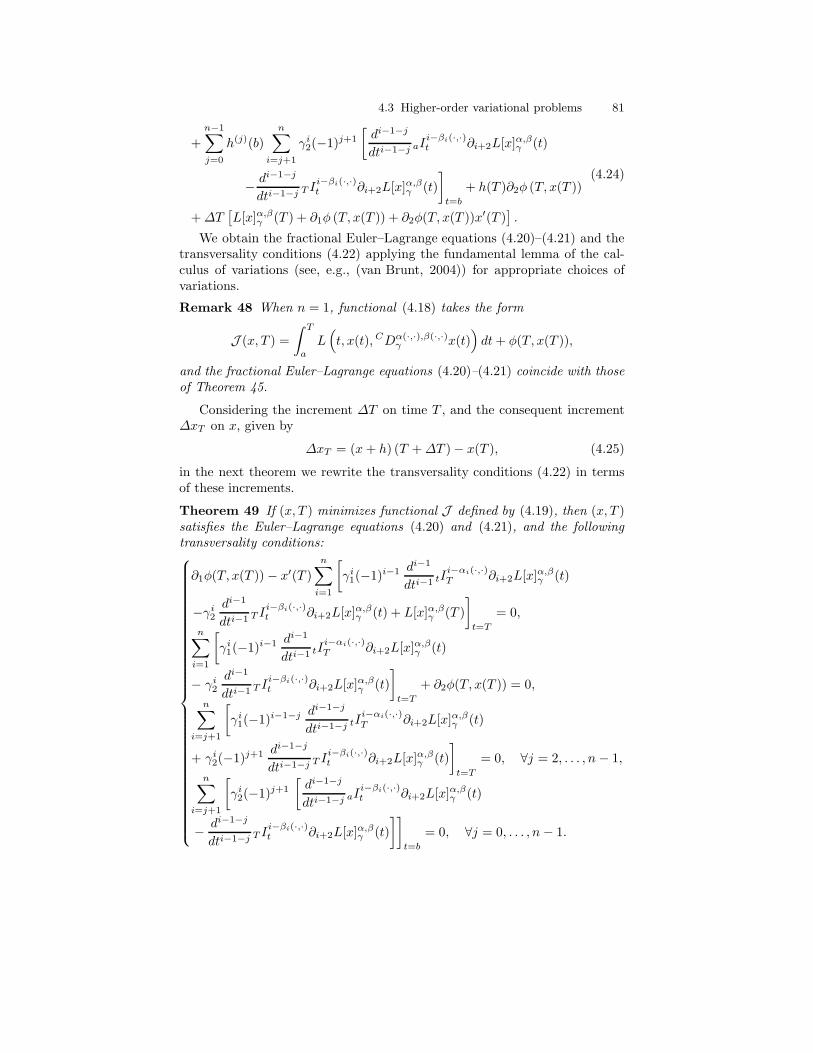
4.3 Higher-order variational problems 81
+
n−1∑
j=0
h(j)(b)
n∑
i=j+1
γi2(−1)j+1
[
di−1−j
dti−1−j aIi−βi(·,·)t ∂i+2L[x]
α,βγ (t)
− di−1−j
dti−1−j T Ii−βi(·,·)t ∂i+2L[x]
α,βγ (t)
]
t=b
+ h(T )∂2φ (T, x(T ))
+∆T[
L[x]α,βγ (T ) + ∂1φ (T, x(T )) + ∂2φ(T, x(T ))x′(T )
]
.
(4.24)
We obtain the fractional Euler–Lagrange equations (4.20)–(4.21) and thetransversality conditions (4.22) applying the fundamental lemma of the cal-culus of variations (see, e.g., (van Brunt, 2004)) for appropriate choices ofvariations.
Remark 48 When n = 1, functional (4.18) takes the form
J (x, T ) =
∫ T
a
L(
t, x(t),CDα(·,·),β(·,·)γ x(t)
)
dt+ φ(T, x(T )),
and the fractional Euler–Lagrange equations (4.20)–(4.21) coincide with thoseof Theorem 45.
Considering the increment ∆T on time T , and the consequent increment∆xT on x, given by
∆xT = (x+ h) (T +∆T )− x(T ), (4.25)
in the next theorem we rewrite the transversality conditions (4.22) in termsof these increments.
Theorem 49 If (x, T ) minimizes functional J defined by (4.19), then (x, T )satisfies the Euler–Lagrange equations (4.20) and (4.21), and the followingtransversality conditions:
∂1φ(T, x(T ))− x′(T )
n∑
i=1
[
γi1(−1)i−1 di−1
dti−1 tIi−αi(·,·)T ∂i+2L[x]
α,βγ (t)
−γi2di−1
dti−1 T Ii−βi(·,·)t ∂i+2L[x]
α,βγ (t) + L[x]α,βγ (T )
]
t=T
= 0,
n∑
i=1
[
γi1(−1)i−1 di−1
dti−1 tIi−αi(·,·)T ∂i+2L[x]
α,βγ (t)
− γi2di−1
dti−1 T Ii−βi(·,·)t ∂i+2L[x]
α,βγ (t)
]
t=T
+ ∂2φ(T, x(T )) = 0,
n∑
i=j+1
[
γi1(−1)i−1−j di−1−j
dti−1−j tIi−αi(·,·)T ∂i+2L[x]
α,βγ (t)
+ γi2(−1)j+1 di−1−j
dti−1−j T Ii−βi(·,·)t ∂i+2L[x]
α,βγ (t)
]
t=T
= 0, ∀j = 2, . . . , n− 1,
n∑
i=j+1
[
γi2(−1)j+1
[
di−1−j
dti−1−j aIi−βi(·,·)t ∂i+2L[x]
α,βγ (t)
− di−1−j
dti−1−j T Ii−βi(·,·)t ∂i+2L[x]
α,βγ (t)
]]
t=b
= 0, ∀j = 0, . . . , n− 1.

82 4 The fractional calculus of variations
Proof. Using Taylor’s expansion up to first order, and restricting the set ofvariations to those for which h′(T ) = 0, we obtain that
(x+ h) (T +∆T ) = (x+ h)(T ) + x′(T )∆T +O(∆T )2.
According to the increment on x given by (4.25), we get
h(T ) = ∆xT − x′(T )∆T +O(∆T )2.
From substitution of this expression into (4.24), and by using appropriatechoices of variations, we obtain the intended transversality conditions.
4.3.2 Example
We provide an illustrative example. It is covered by Theorem 47 .Let pn−1(t) be a polynomial of degree n − 1. If α, β : [0, b]2 → (n − 1, n)
are the fractional orders, then CDα(·,·),β(·,·)γ pn−1(t) = 0 since p
(n)n−1(t) = 0 for
all t. Consider the functional
J (x, T ) =
∫ T
0
[
(
CDα(·,·),β(·,·)γ x(t)
)2
+ (x(t) − pn−1(t))2 − t− 1
]
dt+ T 2
subject to the initial constraints
x(0) = pn−1(0) and x(k)(0) = p(k)n−1(0), k = 1, . . . , n− 1.
Observe that, for all t ∈ [0, b],
∂iL[pn−1]α,βγ (t) = 0, i = 2, 3.
Thus, function x ≡ pn−1 and the final time T = 1 satisfy the necessaryoptimality conditions of Theorem 47. We also remark that, for any curve x,one has
J (x, T ) ≥∫ T
0
[−t− 1] dt+ T 2 =T 2
2− T,
which attains a minimum value −1/2 at T = 1. Since J (pn−1, 1) = −1/2, weconclude that (pn−1, 1) is the (global) minimizer of J .
4.4 Variational problems with time delay
In this section, we consider fractional variational problems with time delay.As mentioned in (Machado, 2011), “we verify that a fractional derivative re-quires an infinite number of samples capturing, therefore, all the signal his-tory, contrary to what happens with integer order derivatives that are merelylocal operators. This fact motivates the evaluation of calculation strategies
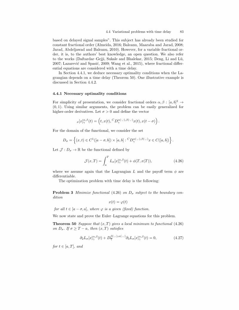
4.4 Variational problems with time delay 83
based on delayed signal samples”. This subject has already been studied forconstant fractional order (Almeida, 2016; Baleanu, Maaraba and Jarad, 2008;Jarad, Abdeljawad and Baleanu, 2010). However, for a variable fractional or-der, it is, to the authors’ best knowledge, an open question. We also referto the works (Daftardar–Gejji, Sukale and Bhalekar, 2015; Deng, Li and Lu,2007; Lazarevic and Spasic, 2009; Wang et al., 2015), where fractional differ-ential equations are considered with a time delay.
In Section 4.4.1, we deduce necessary optimality conditions when the La-grangian depends on a time delay (Theorem 50). One illustrative example isdiscussed in Section 4.4.2.
4.4.1 Necessary optimality conditions
For simplicity of presentation, we consider fractional orders α, β : [a, b]2 →(0, 1). Using similar arguments, the problem can be easily generalized forhigher-order derivatives. Let σ > 0 and define the vector
σ[x]α,βγ (t) =
(
t, x(t),CDα(·,·),β(·,·)γ x(t), x(t − σ)
)
.
For the domain of the functional, we consider the set
Dσ =
(x, t) ∈ C1([a− σ, b])× [a, b] : CDα(·,·),β(·,·)γ x ∈ C([a, b])
.
Let J : Dσ → R be the functional defined by
J (x, T ) =
∫ T
a
Lσ[x]α,βγ (t) + φ(T, x(T )), (4.26)
where we assume again that the Lagrangian L and the payoff term φ aredifferentiable.
The optimization problem with time delay is the following:
Problem 3 Minimize functional (4.26) on Dσ subject to the boundary con-dition
x(t) = ϕ(t)
for all t ∈ [a− σ, a], where ϕ is a given (fixed) function.
We now state and prove the Euler–Lagrange equations for this problem.
Theorem 50 Suppose that (x, T ) gives a local minimum to functional (4.26)on Dσ. If σ ≥ T − a, then (x, T ) satisfies
∂2Lσ[x]α,βγ (t) +D
β(·,·),α(·,·)γ ∂3Lσ[x]
α,βγ (t) = 0, (4.27)
for t ∈ [a, T ], and

84 4 The fractional calculus of variations
γ2
(
aDβ(·,·)t ∂3Lσ[x]
α,βγ (t)− TD
β(·,·)t ∂3Lσ[x]
α,βγ (t)
)
= 0, (4.28)
for t ∈ [T, b]. Moreover, (x, T ) satisfies
Lσ[x]α,βγ (T ) + ∂1φ(T, x(T )) + ∂2φ(T, x(T ))x
′(T ) = 0,[
γ1 tI1−α(·,·)T ∂3Lσ[x]
α,βγ (t)− γ2 T I
1−β(·,·)t ∂3Lσ[x]
α,βγ (t)
]
t=T
+∂2φ(T, x(T )) = 0,
γ2
[
T I1−β(·,·)t ∂3Lσ[x]
α,βγ (t)− aI
1−β(·,·)t ∂3Lσ[x]
α,βγ (t)
]
t=b= 0.
(4.29)
If σ < T − a, then Eq. (4.27) is replaced by the two following ones:
∂2Lσ[x]α,βγ (t) +D
β(·,·),α(·,·)γ ∂3Lσ[x]
α,βγ (t) + ∂4Lσ[x]
α,βγ (t+ σ) = 0, (4.30)
for t ∈ [a, T − σ], and
∂2Lσ[x]α,βγ (t) +D
β(·,·),α(·,·)γ ∂3Lσ[x]
α,βγ (t) = 0, (4.31)
for t ∈ [T − σ, T ].
Proof. Consider variations of the solution (x+ ǫh, T + ǫ∆T ), where h ∈C1([a − σ, b];R) is such that h(t) = 0 for all t ∈ [a − σ, a], and ǫ,T aretwo reals. If we define j(ǫ) = J (x+ ǫh, T + ǫ∆T ), then j′(0) = 0, that is,
∫ T
a
(
∂2Lσ[x]α,βγ (t)h(t) + ∂3Lσ[x]
α,βγ (t)CDα(·,·),β(·,·)
γ h(t)
+ ∂4Lσ[x]α,βγ (t)h(t− σ)
)
dt+ Lσ[x]α,βγ (T )∆T
+ ∂1φ (T, x(T ))∆T + ∂2φ(T, x(T )) [h(T ) + x′(T )T ] = 0. (4.32)
First, suppose that σ ≥ T − a. In this case, since
∫ T
a
∂4Lσ[x]α,βγ (t)h(t− σ) dt =
∫ T−σ
a−σ
∂4Lσ[x]α,βγ (t+ σ)h(t) dt
and h ≡ 0 on [a−σ, a], this term vanishes in (4.32) and we obtain Eq. (4.12).The rest of the proof is similar to the one presented in Section 4.2, Theorem45, and we obtain (4.27)–(4.29). Suppose now that σ < T − a. In this case,we have that
∫ T
a
∂4Lσ[x]α,βγ (t)h(t− σ) dt =
∫ T−σ
a−σ
∂4Lσ[x]α,βγ (t+ σ)h(t) dt
=
∫ T−σ
a
∂4Lσ[x]α,βγ (t+ σ)h(t) dt.
Next, we evaluate the integral

4.4 Variational problems with time delay 85
∫ T
a
∂3Lσ[x]α,βγ (t)CDα(·,·),β(·,·)
γ h(t) dt
=
∫ T−σ
a
∂3Lσ[x]α,βγ (t)CDα(·,·),β(·,·)
γ h(t) dt
+
∫ T
T−σ
∂3Lσ[x]α,βγ (t)CDα(·,·),β(·,·)
γ h(t) dt.
For the first integral, integrating by parts, we have∫ T−σ
a
∂3Lσ[x]α,βγ (t)CDα(·,·),β(·,·)
γ h(t) dt = γ1
∫ T−σ
a
∂3Lσ[x]α,βγ (t)CaD
α(·,·)t h(t)dt
+ γ2
[
∫ b
a
∂3Lσ[x]α,βγ (t)Ct D
β(·,·)b h(t)dt−
∫ b
T−σ
∂3Lσ[x]α,βγ (t)Ct D
β(·,·)b h(t)dt
]
=
∫ T−σ
a
h(t)[
γ1tDα(·,·)T−σ ∂3Lσ[x]
α,βγ (t) + γ2aD
β(·,·)t ∂3Lσ[x]
α,βγ (t)
]
dt
+
∫ b
T−σ
γ2h(t)[
aDβ(·,·)t ∂3Lσ[x]
α,βγ (t)− T−σD
β(·,·)t ∂3Lσ[x]
α,βγ (t)
]
dt
+[
h(t)[
γ1tI1−α(·,·)T−σ ∂3Lσ[x]
α,βγ (t)− γ2T−σI
1−β(·,·)t ∂3Lσ[x]
α,βγ (t)
]]
t=T−σ
+[
γ2h(t)[
−aI1−β(·,·)t ∂3Lσ[x]
α,βγ (t) + T−σI
1−β(·,·)t ∂3Lσ[x]
α,βγ (t)
]]
t=b.
For the second integral, in a similar way, we deduce that∫ T
T−σ
∂3Lσ[x]α,βγ (t)CDα(·,·),β(·,·)
γ h(t) dt
= γ1
[
∫ T
a
∂3Lσ[x]α,βγ (t)CaD
α(·,·)t h(t)dt−
∫ T−σ
a
∂3Lσ[x]α,βγ (t)CaD
α(·,·)t h(t)dt
]
+ γ2
[
∫ b
T−σ
∂3Lσ[x]α,βγ (t)Ct D
β(·,·)b h(t)dt−
∫ b
T
∂3Lσ[x]α,βγ (t)Ct D
β(·,·)b h(t)dt
]
=
∫ T−σ
a
γ1h(t)[
tDα(·,·)T ∂3Lσ[x]
α,βγ (t)− tD
α(·,·)T−σ ∂3Lσ[x]
α,βγ (t)
]
dt
+
∫ T
T−σ
h(t)[
γ1tDα(·,·)T ∂3Lσ[x]
α,βγ (t) + γ2T−σD
β(·,·)t ∂3Lσ[x]
α,βγ (t)
]
dt
+
∫ b
T
γ2h(t)[
T−σDβ(·,·)t ∂3Lσ[x]
α,βγ (t)− TD
β(·,·)t ∂3Lσ[x]
α,βγ (t)
]
dt
+[
h(t)[
−γ1tI1−α(·,·)T−σ ∂3Lσ[x]
α,βγ (t) + γ2T−σI
1−β(·,·)t ∂3Lσ[x]
α,βγ (t)
]]
t=T−σ
+[
h(t)[
γ1tI1−α(·,·)T ∂3Lσ[x]
α,βγ (t)− γ2T I
1−β(·,·)t ∂3Lσ[x]
α,βγ (t)
]]
t=T
+[
γ2h(t)[
−T−σI1−β(·,·)t ∂3Lσ[x]
α,βγ (t) + T I
1−β(·,·)t ∂3Lσ[x]
α,βγ (t)
]]
t=b.
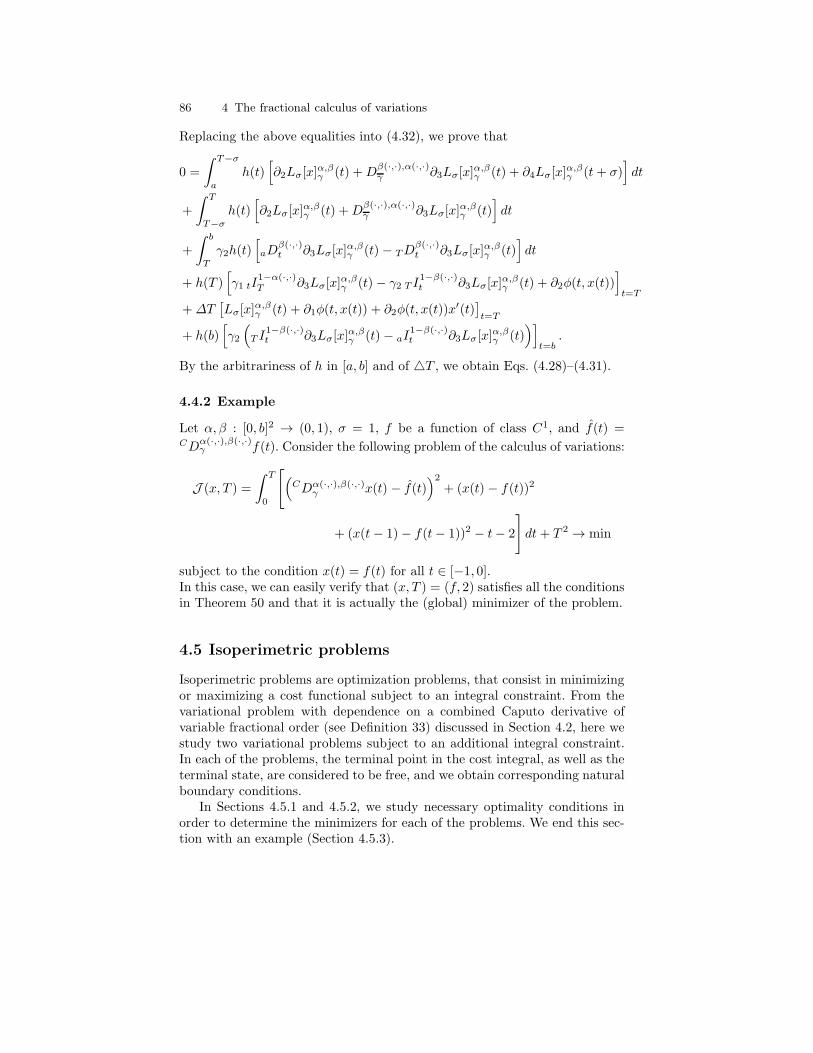
86 4 The fractional calculus of variations
Replacing the above equalities into (4.32), we prove that
0 =
∫ T−σ
a
h(t)[
∂2Lσ[x]α,βγ (t) +D
β(·,·),α(·,·)γ ∂3Lσ[x]
α,βγ (t) + ∂4Lσ[x]
α,βγ (t+ σ)
]
dt
+
∫ T
T−σ
h(t)[
∂2Lσ[x]α,βγ (t) +D
β(·,·),α(·,·)γ ∂3Lσ[x]
α,βγ (t)
]
dt
+
∫ b
T
γ2h(t)[
aDβ(·,·)t ∂3Lσ[x]
α,βγ (t)− TD
β(·,·)t ∂3Lσ[x]
α,βγ (t)
]
dt
+ h(T )[
γ1 tI1−α(·,·)T ∂3Lσ[x]
α,βγ (t)− γ2 T I
1−β(·,·)t ∂3Lσ[x]
α,βγ (t) + ∂2φ(t, x(t))
]
t=T
+∆T[
Lσ[x]α,βγ (t) + ∂1φ(t, x(t)) + ∂2φ(t, x(t))x
′(t)]
t=T
+ h(b)[
γ2
(
T I1−β(·,·)t ∂3Lσ[x]
α,βγ (t)− aI
1−β(·,·)t ∂3Lσ[x]
α,βγ (t)
)]
t=b.
By the arbitrariness of h in [a, b] and of T , we obtain Eqs. (4.28)–(4.31).
4.4.2 Example
Let α, β : [0, b]2 → (0, 1), σ = 1, f be a function of class C1, and f(t) =CD
α(·,·),β(·,·)γ f(t). Consider the following problem of the calculus of variations:
J (x, T ) =
∫ T
0
[
(
CDα(·,·),β(·,·)γ x(t) − f(t)
)2
+ (x(t) − f(t))2
+ (x(t− 1)− f(t− 1))2 − t− 2
]
dt+ T 2 → min
subject to the condition x(t) = f(t) for all t ∈ [−1, 0].In this case, we can easily verify that (x, T ) = (f, 2) satisfies all the conditionsin Theorem 50 and that it is actually the (global) minimizer of the problem.
4.5 Isoperimetric problems
Isoperimetric problems are optimization problems, that consist in minimizingor maximizing a cost functional subject to an integral constraint. From thevariational problem with dependence on a combined Caputo derivative ofvariable fractional order (see Definition 33) discussed in Section 4.2, here westudy two variational problems subject to an additional integral constraint.In each of the problems, the terminal point in the cost integral, as well as theterminal state, are considered to be free, and we obtain corresponding naturalboundary conditions.
In Sections 4.5.1 and 4.5.2, we study necessary optimality conditions inorder to determine the minimizers for each of the problems. We end this sec-tion with an example (Section 4.5.3).

4.5 Isoperimetric problems 87
For the two isoperimetric problems considered in the next sections, let Dbe the set given by (4.6) and [x]α,βγ (t) the vector (4.8).
Picking up the problem of the fractional calculus of variations withvariable-order, discussed in Section 4.2, we consider also a differentiable La-grangian L : [a, b]× R
2 → R and the functional J : D → R of the form
J (x, T ) =
∫ T
a
L[x]α,βγ (t)dt+ φ(T, x(T )), (4.33)
where the terminal cost function φ : [a, b]× R → R is of class C1.In the sequel, we need the auxiliary notation of the dual fractional deriva-
tive:
Dβ(·,·),α(·,·)γ,c = γ2 aD
β(·,·)t + γ1 tD
α(·,·)c , where γ = (γ2, γ1) and c ∈ (a, b].
(4.34)With the functional J , defined by (4.33), we consider two different isoperi-
metrics problems.
4.5.1 Necessary optimality conditions I
The first fractional isoperimetric problem of the calculus of variations is Prob-lem 4.
Problem 4 Determine the local minimizers of J over all (x, T ) ∈ D satisfy-ing a boundary condition
x(a) = xa (4.35)
for a fixed xa ∈ R and an integral constraint of the form
∫ T
a
g[x]α,βγ (t)dt = ψ(T ), (4.36)
where g : C1(
[a, b]× R2)
→ R and ψ : [a, b] → R are two differentiablefunctions. The terminal time T and terminal state x(T ) are free.
In this problem, the condition of the form (4.36) is called an isoperimetricconstraint. The next theorem gives fractional necessary optimality conditionsfor Problem 4.
Theorem 51 Suppose that (x, T ) gives a local minimum for functional (4.33)on D subject to the boundary condition (4.35) and the isoperimetric constraint(4.36). If (x, T ) does not satisfy the Euler–Lagrange equations with respect tothe isoperimetric constraint, that is, if one of the two following conditions arenot verified,
∂2g[x]α,βγ (t) +D
β(·,·),α(·,·)γ,T ∂3g[x]
α,βγ (t) = 0, t ∈ [a, T ], (4.37)
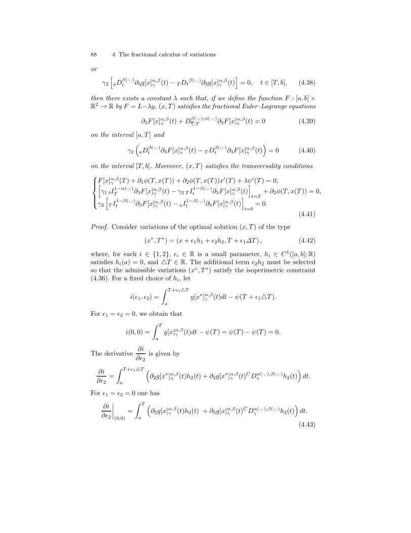
88 4 The fractional calculus of variations
or
γ2
[
aDβ(·,·)t ∂3g[x]
α,βγ (t)− TDt
β(·,·)∂3g[x]α,βγ (t)
]
= 0, t ∈ [T, b], (4.38)
then there exists a constant λ such that, if we define the function F : [a, b]×R
2 → R by F = L−λg, (x, T ) satisfies the fractional Euler–Lagrange equations
∂2F [x]α,βγ (t) +D
β(·,·),α(·,·)γ,T ∂3F [x]
α,βγ (t) = 0 (4.39)
on the interval [a, T ] and
γ2
(
aDβ(·,·)t ∂3F [x]
α,βγ (t)− TD
β(·,·)t ∂3F [x]
α,βγ (t)
)
= 0 (4.40)
on the interval [T, b]. Moreover, (x, T ) satisfies the transversality conditions
F [x]α,βγ (T ) + ∂1φ(T, x(T )) + ∂2φ(T, x(T ))x′(T ) + λψ′(T ) = 0,
[
γ1 tI1−α(·,·)T ∂3F [x]
α,βγ (t)− γ2 T I
1−β(·,·)t ∂3F [x]
α,βγ (t)
]
t=T+ ∂2φ(T, x(T )) = 0,
γ2
[
T I1−β(·,·)t ∂3F [x]
α,βγ (t)− aI
1−β(·,·)t ∂3F [x]
α,βγ (t)
]
t=b= 0.
(4.41)
Proof. Consider variations of the optimal solution (x, T ) of the type
(x∗, T ∗) = (x+ ǫ1h1 + ǫ2h2, T + ǫ1∆T ) , (4.42)
where, for each i ∈ 1, 2, ǫi ∈ R is a small parameter, hi ∈ C1([a, b];R)satisfies hi(a) = 0, and T ∈ R. The additional term ǫ2h2 must be selectedso that the admissible variations (x∗, T ∗) satisfy the isoperimetric constraint(4.36). For a fixed choice of hi, let
i(ǫ1, ǫ2) =
∫ T+ǫ1T
a
g[x∗]α,βγ (t)dt− ψ(T + ǫ1T ).
For ǫ1 = ǫ2 = 0, we obtain that
i(0, 0) =
∫ T
a
g[x]α,βγ (t)dt − ψ(T ) = ψ(T )− ψ(T ) = 0.
The derivative∂i
∂ǫ2is given by
∂i
∂ǫ2=
∫ T+ǫ1T
a
(
∂2g[x∗]α,βγ (t)h2(t) + ∂3g[x
∗]α,βγ (t)CDα(·,·),β(·,·)γ h2(t)
)
dt.
For ǫ1 = ǫ2 = 0 one has
∂i
∂ǫ2
∣
∣
∣
∣
(0,0)
=
∫ T
a
(
∂2g[x]α,βγ (t)h2(t) + ∂3g[x]
α,βγ (t)CDα(·,·),β(·,·)
γ h2(t))
dt.
(4.43)

4.5 Isoperimetric problems 89
The second term in (4.43) can be written as
∫ T
a
∂3g[x]α,βγ (t)CDα(·,·),β(·,·)
γ h2(t)dt
=
∫ T
a
∂3g[x]α,βγ (t)
[
γ1CaD
α(·,·)t h2(t) + γ2
Ct D
β(·,·)b h2(t)
]
dt
= γ1
∫ T
a
∂3g[x]α,βγ (t)CaD
α(·,·)t h2(t)dt
+ γ2
[
∫ b
a
∂3g[x]α,βγ (t)Ct D
β(·,·)b h2(t)dt −
∫ b
T
∂3g[x]α,βγ (t)Ct D
β(·,·)b h2(t)dt
]
.
(4.44)
Using the fractional integrating by parts formula, (4.44) is equal to
∫ T
a
h2(t)[
γ1tDTα(·,·)∂3g[x]
α,βγ (t) + γ2aDt
β(·,·)∂3g[x]α,βγ (t)
]
dt
+
∫ b
T
γ2h2(t)[
aDβ(·,·)t ∂3g[x]
α,βγ (t)− TDt
β(·,·)∂3g[x]α,βγ (t)
]
dt
+
[
h2(t)
(
γ1tIT1−α(·,·)∂3g[x]
α,βγ (t)− γ2T It
1−β(·,·)∂3g[x]α,βγ (t)
)]
t=T
+
[
γ2h2(t)
(
T It1−β(·,·)∂3g[x]
α,βγ (t)− aIt
1−β(·,·)∂3g[x]α,βγ (t)
)]
t=b
.
Substituting these relations into (4.43), and considering the fractional opera-
tor Dβ(·,·),α(·,·)γ,c as defined in (4.34), we obtain that
∂i
∂ǫ2
∣
∣
∣
∣
(0,0)
=
∫ T
a
h2(t)[
∂2g[x]α,βγ (t) +D
β(·,·),α(·,·)γ,T ∂3g[x]
α,βγ (t)
]
dt
+
∫ b
T
γ2h2(t)[
aDβ(·,·)t ∂3g[x]
α,βγ (t)− TDt
β(·,·)∂3g[x]α,βγ (t)
]
dt
+
[
h2(t)
(
γ1tIT1−α(·,·)∂3g[x]
α,βγ (t)− γ2T It
1−β(·,·)∂3g[x]α,βγ (t)
)]
t=T
+
[
γ2h2(t)
(
T It1−β(·,·)∂3g[x]
α,βγ (t)− aIt
1−β(·,·)∂3g[x]α,βγ (t)
)]
t=b
.
Since (4.37) or (4.38) fails, there exists a function h2 such that
∂i
∂ǫ2
∣
∣
∣
∣
(0,0)
6= 0.

90 4 The fractional calculus of variations
In fact, if not, from the arbitrariness of the function h2 and the fundamentallemma of the calculus of the variations, (4.37) and (4.38) would be verified.Thus, we may apply the implicit function theorem, that ensures the existenceof a function ǫ2(·), defined in a neighborhood of zero, such that i(ǫ1, ǫ2(ǫ1)) =0. In conclusion, there exists a subfamily of variations of the form (4.42) thatverifies the integral constraint (4.36). We now seek to prove the main result.For that purpose, consider the auxiliary function j(ǫ1, ǫ2) = J (x∗, T ∗).
By hypothesis, function j attains a local minimum at (0, 0) when subjectto the constraint i(·, ·) = 0, and we proved before that ∇i(0, 0) 6= (0, 0).Applying the Lagrange multiplier rule, we ensure the existence of a numberλ such that
∇ (j(0, 0)− λi(0, 0)) = (0, 0).
In particular,∂ (j − λi)
∂ǫ1(0, 0) = 0. (4.45)
Let F = L− λg. The relation (4.45) can be written as
0 =
∫ T
a
h1(t)[
∂2F [x]α,βγ (t) +D
β(·,·),α(·,·)γ,T ∂3F [x]
α,βγ (t)
]
dt
+
∫ b
T
γ2h1(t)[
aDβ(·,·)t ∂3F [x]
α,βγ (t)− TD
β(·,·)t ∂3F [x]
α,βγ (t)
]
dt
+ h1(T )[
γ1 tI1−α(·,·)T ∂3F [x]
α,βγ (t)− γ2 T I
1−β(·,·)t ∂3F [x]
α,βγ (t) + ∂2φ(t, x(t))
]
t=T
+∆T[
F [x]α,βγ (t) + ∂1φ(t, x(t)) + ∂2φ(t, x(t))x′(t) + λψ′(t)
]
t=T
+ h1(b)γ2
[
T I1−β(·,·)t ∂3F [x]
α,βγ (t)− aI
1−β(·,·)t ∂3F [x]
α,βγ (t)
]
t=b.
(4.46)
As h1 and T are arbitrary, we can choose T = 0 and h1(t) = 0 for allt ∈ [T, b]. But h1 is arbitrary in t ∈ [a, T ). Then, we obtain the first necessarycondition (4.39):
∂2F [x]α,βγ (t) +D
β(·,·),α(·,·)γ,T ∂3F [x]
α,βγ (t) = 0 ∀t ∈ [a, T ].
Analogously, considering T = 0 and h1(t) = 0 for all t ∈ [a, T ] ∪ b, andh1 arbitrary on (T, b), we obtain the second necessary condition (4.40):
γ2
(
aDβ(·,·)t ∂3F [x]
α,βγ (t)− TD
β(·,·)t ∂3F [x]
α,βγ (t)
)
= 0 ∀t ∈ [T, b].
As (x, T ) is a solution to the necessary conditions (4.39) and (4.40), thenequation (4.46) takes the form

4.5 Isoperimetric problems 91
h1(T )[
γ1 tI1−α(·,·)T ∂3F [x]
α,βγ (t)− γ2 T I
1−β(·,·)t ∂3F [x]
α,βγ (t) + ∂2φ(t, x(t))
]
t=T
+∆T[
F [x]α,βγ (t) + ∂1φ(t, x(t)) + ∂2φ(t, x(t))x′(t) + λψ′(t)
]
t=T
+ h1(b)[
γ2
(
T I1−β(·,·)t ∂3F [x]
α,βγ (t)− aI
1−β(·,·)t ∂3F [x]
α,βγ (t)
)]
t=b= 0.
(4.47)
Transversality conditions (4.41) are obtained for appropriate choices of vari-ations.
In the next theorem, considering the same Problem 4, we rewrite thetransversality conditions (4.41) in terms of the increment on time ∆T andon the increment of space ∆xT given by
∆xT = (x + h1)(T +∆T )− x(T ). (4.48)
Theorem 52 Let (x, T ) be a local minimizer to the functional (4.33) onD subject to the boundary condition (4.35) and the isoperimetric constraint(4.36). Then (x, T ) satisfies the transversality conditions
F [x]α,βγ (T ) + ∂1φ(T, x(T )) + λψ′(T )
+x′(T )[
γ2T I1−β(·,·)t ∂3F [x]
α,βγ (t)− γ1tI
1−α(·,·)T ∂3F [x]
α,βγ (t)
]
t=T= 0,
[
γ1 tI1−α(·,·)T ∂3F [x]
α,βγ (t)− γ2 T I
1−β(·,·)t ∂3F [x]
α,βγ (t)
]
t=T+ ∂2φ(T, x(T )) = 0,
γ2
[
T I1−β(·,·)t ∂3F [x]
α,βγ (t)− aI
1−β(·,·)t ∂3F [x]
α,βγ (t)
]
t=b= 0.
(4.49)
Proof. Suppose (x∗, T ∗) is an admissible variation of the form (4.42) withǫ1 = 1 and ǫ2 = 0. Using Taylor’s expansion up to first order for a small ∆T ,and restricting the set of variations to those for which h′1(T ) = 0, we obtainthe increment ∆xT on x:
(x + h1) (T +∆T ) = (x+ h1)(T ) + x′(T )∆T + O(∆T )2.
Relation (4.48) allows us to express h1(T ) in terms of ∆T and ∆xT :
h1(T ) = ∆xT − x′(T )∆T +O(∆T )2.
Substituting this expression into (4.47), and using appropriate choices of vari-ations, we obtain the new transversality conditions (4.49).
Theorem 53 Suppose that (x, T ) gives a local minimum for functional (4.33)on D subject to the boundary condition (4.35) and the isoperimetric constraint(4.36). Then, there exists (λ0, λ) 6= (0, 0) such that, if we define the functionF : [a, b]× R
2 → R by F = λ0L − λg, (x, T ) satisfies the following fractionalEuler–Lagrange equations:
∂2F [x]α,βγ (t) +D
β(·,·),α(·,·)γ,T ∂3F [x]
α,βγ (t) = 0

92 4 The fractional calculus of variations
on the interval [a, T ], and
γ2
(
aDβ(·,·)t ∂3F [x]
α,βγ (t)− TD
β(·,·)t ∂3F [x]
α,βγ (t)
)
= 0
on the interval [T, b].
Proof. If (x, T ) does not verifies (4.37) or (4.38), then the hypothesis of The-orem 51 is satisfied and we prove Theorem 53 considering λ0 = 1. If (x, T )verifies (4.37) and (4.38), then we prove the result by considering λ = 1 andλ0 = 0.
4.5.2 Necessary optimality conditions II
We now consider a new isoperimetric type problem with the isoperimetricconstraint of form
∫ b
a
g[x]α,βγ (t)dt = C, (4.50)
where C is a given real number.
Problem 5 Determine the local minimizers of J (4.33), over all (x, T ) ∈ Dsatisfying a boundary condition
x(a) = xa (4.51)
for a fixed xa ∈ R and an integral constraint of the form (4.50).
In the follow theorem, we give fractional necessary optimality conditionsfor Problem 5.
Theorem 54 Suppose that (x, T ) gives a local minimum for functional (4.33)on D subject to the boundary condition (4.51) and the isoperimetric constraint(4.50). If (x, T ) does not satisfy the Euler–Lagrange equation with respect tothe isoperimetric constraint, that is, the condition
∂2g[x]α,βγ (t) +D
β(·,·),α(·,·)γ,b ∂3g[x]
α,βγ (t) = 0, t ∈ [a, b],
is not satisfied, then there exists λ 6= 0 such that, if we define the functionF : [a, b] × R
2 → R by F = L − λg, (x, T ) satisfies the fractional Euler–Lagrange equations
∂2F [x]α,βγ (t) +D
β(·,·),α(·,·)γ,T ∂3L[x]
α,βγ (t)− λD
β(·,·),α(·,·)γ,b ∂3g[x]
α,βγ (t) = 0 (4.52)
on the interval [a, T ], and
γ2
(
aDβ(·,·)t ∂3F [x]
α,βγ (t)− TD
β(·,·)t ∂3L[x]
α,βγ (t)
)
− λ(
∂2g[x]α,βγ (t) + γ1tD
α(·,·)b ∂3g[x]
α,βγ (t)
)
= 0 (4.53)

4.5 Isoperimetric problems 93
on the interval [T, b]. Moreover, (x, T ) satisfies the transversality conditions
L[x]α,βγ (T ) + ∂1φ(T, x(T )) + ∂2φ(T, x(T ))x′(T ) = 0,
[
γ1 tI1−α(·,·)T ∂3L[x]
α,βγ (t)− γ2 T I
1−β(·,·)t ∂3L[x]
α,βγ (t) + ∂2φ(t, x(t))
]
t=T= 0
[
−λγ1tI1−α(·,·)b ∂3g[x]
α,βγ (t)
+γ2
(
T I1−β(·,·)t ∂3L[x]
α,βγ (t)− aI
1−β(·,·)t ∂3F [x]
α,βγ (t)
)]
t=b= 0.
(4.54)
Proof. Similarly as done to prove Theorem 51, let
(x∗, T ∗) = (x+ ǫ1h1 + ǫ2h2, T + ǫ1∆T )
be a variation of the solution, and define
i(ǫ1, ǫ2) =
∫ b
a
g[x∗]α,βγ (t)dt− C.
The derivative∂i
∂ǫ2, when ǫ1 = ǫ2 = 0, is
∂i
∂ǫ2
∣
∣
∣
∣
(0,0)
=
∫ b
a
(
∂2g[x]α,βγ (t)h2(t) + ∂3g[x]
α,βγ (t)CDα(·,·),β(·,·)
γ h2(t))
dt.
Integrating by parts and choosing variations such that h2(b) = 0, we have
∂i
∂ǫ2
∣
∣
∣
∣
(0, 0) =
∫ b
a
h2(t)[
∂2g[x]α,βγ (t) +D
β(·,·),α(·,·)γ,b ∂3g[x]
α,βγ (t)
]
dt.
Thus, there exists a function h2 such that
∂i
∂ǫ2
∣
∣
∣
∣
(0, 0) 6= 0.
We may apply the implicit function theorem to conclude that there exists asubfamily of variations satisfying the integral constraint. Consider the newfunction j(ǫ1, ǫ2) = J (x∗, T ∗). Since j has a local minimum at (0, 0) whensubject to the constraint i(·, ·) = 0 and ∇i(0, 0) 6= (0, 0), there exists a numberλ such that
∂
∂ǫ1(j − λi) (0, 0) = 0. (4.55)
Let F = L− λg. Relation (4.55) can be written as

94 4 The fractional calculus of variations
∫ T
a
h1(t)[
∂2F [x]α,βγ (t) +D
β(·,·),α(·,·)γ,T ∂3L[x]
α,βγ (t)− λD
β(·,·),α(·,·)γ,b ∂3g[x]
α,βγ (t)
]
dt
+
∫ b
T
h1(t)[
γ2
(
aDβ(·,·)t ∂3F [x]
α,βγ (t)− TD
β(·,·)t ∂3L[x]
α,βγ (t)
)
− λ(
∂2g[x]α,βγ (t) + γ1tD
α(·,·)b ∂3g[x]
α,βγ (t)
)]
dt
+ h1(T )[
γ1 tI1−α(·,·)T ∂3L[x]
α,βγ (t)− γ2 T I
1−β(·,·)t ∂3L[x]
α,βγ (t) + ∂2φ(t, x(t))
]
t=T
+∆T[
L[x]α,βγ (t) + ∂1φ(t, x(t)) + ∂2φ(t, x(t))x′(t)]
t=T
+ h1(b)[
−λγ1tI1−α(·,·)b ∂3g[x]
α,βγ (t)
+γ2
(
T I1−β(·,·)t ∂3L[x]
α,βγ (t)− aI
1−β(·,·)t ∂3F [x]
α,βγ (t)
)]
t=b= 0.
Considering appropriate choices of variations, we obtain the first (4.52) andthe second (4.53) necessary optimality conditions, and also the transversalityconditions (4.54).
Similarly to Theorem 53, the following result holds.
Theorem 55 Suppose that (x, T ) gives a local minimum for functional (4.33)on D subject to the boundary condition (4.51) and the isoperimetric constraint(4.50). Then there exists (λ0, λ) 6= (0, 0) such that, if we define the functionF : [a, b] × R
2 → R by F = λ0L − λg, (x, T ) satisfies the fractional Euler–Lagrange equations
∂2F [x]α,βγ (t) +D
β(·,·),α(·,·)γ,T ∂3L[x]
α,βγ (t)− λD
β(·,·),α(·,·)γ,b ∂3g[x]
α,βγ (t) = 0
on the interval [a, T ], and
γ2
(
aDβ(·,·)t ∂3F [x]
α,βγ (t)− TD
β(·,·)t ∂3L[x]
α,βγ (t)
)
− λ(
∂2g[x]α,βγ (t) + γ1tD
α(·,·)b ∂3g[x]
α,βγ (t)
)
= 0
on the interval [T, b].
4.5.3 Example
Let α(t, τ) = α(t) and β(t, τ) = β(τ). Define the function
ψ(T ) =
∫ T
0
(
t1−α(t)
2Γ (2− α(t))+
(b− t)1−β(t)
2Γ (2− β(t))
)2
dt
on the interval [0, b] with b > 0. Consider the functional J defined by

4.6 Variational problems with holonomic constraints 95
J(x, t) =
∫ T
0
[
α(t) +(
CDα(·,·),β(·,·)γ x(t)
)2
+
(
t1−α(t)
2Γ (2− α(t))+
(b− t)1−β(t)
2Γ (2− β(t))
)2]
dt
for t ∈ [0, b] and γ = (1/2, 1/2), subject to the initial condition
x(0) = 0
and the isoperimetric constraint
∫ T
0
CDα(·,·),β(·,·)γ x(t)
(
t1−α(t)
2Γ (2− α(t))+
(b− t)1−β(t)
2Γ (2− β(t))
)2
dt = ψ(T ).
Define F = L− λg with λ = 2, that is,
F = α(t) +
(
CDα(·),β(·)γ x(t) − t1−α(t)
2Γ (2− α(t))− (b − t)1−β(t)
2Γ (2− β(t))
)2
.
Consider the function x(t) = t with t ∈ [0, b]. Because
CDα(·,·),β(·,·)γ x(t) =
t1−α(t)
2Γ (2− α(t))+
(b − t)1−β(t)
2Γ (2− β(t)),
we have that x satisfies conditions (4.39), (4.40) and the two last of (4.41).Using the first condition of (4.41), that is,
α(t) + 2
(
T 1−α(T )
2Γ (2− α(T ))+
(b− T )1−β(T )
2Γ (2− β(T ))
)2
= 0,
we obtain the optimal time T .
4.6 Variational problems with holonomic constraints
In this section, we present a new variational problem subject to a new typeof constraints. A holonomic constraint is a condition of the form
g(t, x) = 0,
where x = (x1, x2, ..., xn), n ≥ 2, and g is a given function (see, e.g.,(van Brunt, 2004)).
Consider the space
U = (x1, x2, T ) ∈ C1([a, b])× C1([a, b])× [a, b] : x1(a) = x1a ∧ x2(a) = x2a(4.56)
for fixed reals x1a, x2a ∈ R. In this section, we consider the following varia-tional problem:

96 4 The fractional calculus of variations
Problem 6 Find functions x1 and x2 that maximize or minimize the func-tional J defined in U by
J (x1, x2, T ) =
∫ T
a
L(t, x1(t), x2(t),CDα(·,·),β(·,·)
γ x1(t),CDα(·,·),β(·,·)
γ x2(t))dt
+ φ(T, x1(T ), x2(T )),
(4.57)
where the admissible functions satisfy the constraint
g(t, x1(t), x2(t)) = 0, t ∈ [a, b], (4.58)
called a holonomic constraint, where g : [a, b] × R2 → R is a continuous
function and continuously differentiable with respect to second and third argu-ments.The terminal time T and terminal states x1(T ) and x2(T ) are free and theLagrangian L : [a, b] × R
4 → R is a continuous function and continuouslydifferentiable with respect to its ith argument, i ∈ 2, 3, 4, 5. The terminalcost function φ : [a, b]× R
2 → R is of class C1.
4.6.1 Necessary optimality conditions
The next theorem gives fractional necessary optimality conditions to the vari-ational problem with a holonomic constraint. To simplify the notation, we de-
note by x the vector (x1, x2); byCD
α(·,·),β(·,·)γ x we mean the two-dimensional
vector (CDα(·,·),β(·,·)γ x1,
CDα(·,·),β(·,·)γ x2); and we use the operator
[x]α,βγ (t) :=(
t, x(t),CDα(·,·),β(·,·)γ x(t)
)
.
The next result given necessary optimality conditions for Problem 6.
Theorem 56 Suppose that (x, T ) gives a local minimum to functional J asin (4.57), under the constraint (4.58) and the boundary conditions defined in(4.56) . If
∂3g(t, x(t)) 6= 0 ∀t ∈ [a, b],
then there exists a piecewise continuous function λ : [a, b] → R such that (x, T )satisfies the following fractional Euler–Lagrange equations:
∂2L[x]α,βγ (t) +D
β(·,·),α(·,·)γ,T ∂4L[x]
α,βγ (t) + λ(t)∂2g(t, x(t)) = 0 (4.59)
and
∂3L[x]α,βγ (t) +D
β(·,·),α(·,·)γ,T ∂5L[x]
α,βγ (t) + λ(t)∂3g(t, x(t)) = 0 (4.60)
on the interval [a, T ], and

4.6 Variational problems with holonomic constraints 97
γ2
(
aDβ(·,·)t ∂4L[x]
α,βγ (t)− TDt
β(·,·)∂4L[x]α,βγ (t) + λ(t)∂2g(t, x(t))
)
= 0
(4.61)and
aDβ(·,·)t ∂5L[x]
α,βγ (t)− TDt
β(·,·)∂5L[x]α,βγ (t) + λ(t)∂3g(t, x(t)) = 0 (4.62)
on the interval [T, b]. Moreover, (x, T ) satisfies the transversality conditions
L[x]α,βγ (T ) + ∂1φ(T, x(T )) + ∂2φ(T, x(T ))x′1(T ) + ∂3φ(T, x(T ))x
′2(T ) = 0,
[
γ1 tI1−α(·,·)T ∂4L[x]
α,βγ (t)− γ2 T I
1−β(·,·)t ∂4L[x]
α,βγ (t)
]
t=T+ ∂2φ(T, x(T )) = 0,
[
γ1tIT1−α(·,·)∂5L[x]
α,βγ (t)− γ2T It
1−β(·,·)∂5L[x]α,βγ (t)
]
t=T+ ∂3φ(T, x(T )) = 0,
γ2
[
T I1−β(·,·)t ∂4L[x]
α,βγ (t)− aI
1−β(·,·)t ∂4L[x]
α,βγ (t)
]
t=b= 0,
γ2
[
T I1−β(·,·)t ∂5L[x]
α,βγ (t)− aI
1−β(·,·)t ∂5L[x]
α,βγ (t)
]
t=b= 0.
(4.63)
Proof. Consider admissible variations of the optimal solution (x, T ) of thetype
(x∗, T ∗) = (x+ ǫh, T + ǫ∆T ) ,
where ǫ ∈ R is a small parameter, h = (h1, h2) ∈ C1([a, b])×C1([a, b]) satisfieshi(a) = 0, i = 1, 2, and T ∈ R. Because
∂3g(t, x(t)) 6= 0 ∀t ∈ [a, b],
by the implicit function theorem there exists a subfamily of variations of (x, T )that satisfy (4.58), that is, there exists a unique function h2(ǫ, h1) such thatthe admissible variation (x∗, T ∗) satisfies the holonomic constraint (4.58):
g(t, x1(t) + ǫh1(t), x2(t) + ǫh2(t)) = 0 ∀t ∈ [a, b].
Differentiating this condition with respect to ǫ and considering ǫ = 0, weobtain that
∂2g(t, x(t))h1(t) + ∂3g(t, x(t))h2(t) = 0,
which is equivalent to
∂2g(t, x(t))h1(t)
∂3g(t, x(t))= −h2(t). (4.64)
Define j on a neighbourhood of zero by
j(ǫ) =
∫ T+ǫT
a
L[x∗]α,βγ (t)dt+ φ(T + ǫT, x∗(T + ǫT )).
The derivative∂j
∂ǫfor ǫ = 0 is

98 4 The fractional calculus of variations
∂j
∂ǫ
∣
∣
∣
∣
ǫ=0
=
∫ T
a
(
∂2L[x]α,βγ (t)h1(t) + ∂3L[x]
α,βγ (t)h2(t)
+∂4L[x]α,βγ (t)CDα(·,·),β(·,·)
γ h1(t) + ∂5L[x]α,βγ (t)CDα(·,·),β(·,·)
γ h2(t))
dt
+ L[x]α,βγ (T )T + ∂1φ(T, x(T ))T + ∂2φ(T, x(T )) [h1(T ) + x′1(T )T ]+ ∂3φ(T, x(T )) [h2(T ) + x′2(T )T ] .
(4.65)
The third term in (4.65) can be written as
∫ T
a
∂4L[x]α,βγ (t)CDα(·,·),β(·,·)
γ h1(t)dt
=
∫ T
a
∂4L[x]α,βγ (t)
[
γ1CaD
α(·,·)t h1(t) + γ2
Ct D
β(·,·)b h1(t)
]
dt
= γ1
∫ T
a
∂4L[x]α,βγ (t)CaD
α(·,·)t h1(t)dt
+ γ2
[
∫ b
a
∂4L[x]α,βγ (t)Ct D
β(·,·)b h1(t)dt −
∫ b
T
∂4L[x]α,βγ (t)Ct D
β(·,·)b h1(t)dt
]
.
(4.66)
Integrating by parts, (4.66) can be written as
∫ T
a
h1(t)[
γ1tDTα(·,·)∂4L[x]
α,βγ (t) + γ2aDt
β(·,·)∂4L[x]α,βγ (t)
]
dt
+
∫ b
T
γ2h1(t)[
aDβ(·,·)t ∂4L[x]
α,βγ (t) − TDt
β(·,·)∂4L[x]α,βγ (t)
]
dt
+
[
h1(t)
(
γ1tIT1−α(·,·)∂4L[x]
α,βγ (t)− γ2T It
1−β(·,·)∂4L[x]α,βγ (t)
)]
t=T
+
[
γ2h1(t)
(
T It1−β(·,·)∂4L[x]
α,βγ (t)− aIt
1−β(·,·)∂4L[x]α,βγ (t)
)]
t=b
.
By proceeding similarly to the 4th term in (4.65), we obtain an equivalent ex-pression. Substituting these relations into (4.65) and considering the fractional
operator Dβ(·,·),α(·,·)γ,c as defined in (4.34), we obtain that

4.6 Variational problems with holonomic constraints 99
0 =
∫ T
a
[
h1(t)[
∂2L[x]α,βγ (t) +D
β(·,·),α(·,·)γ,T ∂4L[x]
α,βγ (t)
]
+ h2(t)[
∂3L[x]α,βγ (t) +D
β(·,·),α(·,·)γ,T ∂5L[x]
α,βγ (t)
]
]
dt
+γ2
∫ b
T
[
h1(t)[
aDβ(·,·)t ∂4L[x]
α,βγ (t)− TDt
β(·,·)∂4L[x]α,βγ (t)
]
+ h2(t)[
aDβ(·,·)t ∂5L[x]
α,βγ (t)− TDt
β(·,·)∂5L[x]α,βγ (t)
]
dt
]
+h1(T )
[
γ1tIT1−α(·,·)∂4L[x]
α,βγ (t)
− γ2T It1−β(·,·)∂4L[x]
α,βγ (t) + ∂2φ(t, x(t))
]
t=T
(4.67)
+h2(T )
[
γ1tIT1−α(·,·)∂5L[x]
α,βγ (t)− γ2T It
1−β(·,·)∂5L[x]α,βγ (t) + ∂3φ(t, x(t))
]
t=T
+T[
L[x]α,βγ (t) + ∂1φ(t, x(t)) + ∂2φ(t, x(t))x′1(t) + ∂3φ(t, x(t))x
′2(t)
]
t=T
+h1(b)
[
γ2
(
T It1−β(·,·)∂4L[x]
α,βγ (t)− aIt
1−β(·,·)∂4L[x]α,βγ (t)
)]
t=b
+h2(b)
[
γ2
(
T It1−β(·,·)∂5L[x]
α,βγ (t)− aIt
1−β(·,·)∂5L[x]α,βγ (t)
)]
t=b
.
Define the piecewise continuous function λ by
λ(t) =
−∂3L[x]
α,βγ (t) +D
β(·,·),α(·,·)γ,T ∂5L[x]
α,βγ (t)
∂3g(t, x(t)), t ∈ [a, T ]
−aDβ(·,·)t ∂5L[x]
α,βγ (t)−T D
β(·,·)t ∂5L[x]
α,βγ (t)
∂3g(t, x(t)), t ∈ [T, b].
(4.68)
Using equations (4.64) and (4.68), we obtain that
λ(t)∂2g(t, x(t))h1(t)
=
(∂3L[x]α,βγ (t) +D
β(·,·),α(·,·)γ,T ∂5L[x]
α,βγ (t))h2(t), t ∈ [a, T ]
(aDβ(·,·)t ∂5L[x]
α,βγ (t)−T D
β(·,·)t ∂5L[x]
α,βγ (t))h2(t), t ∈ [T, b].
Substituting in (4.67), we have

100 4 The fractional calculus of variations
0 =
∫ T
a
h1(t)[
∂2L[x]α,βγ (t) +D
β(·,·),α(·,·)γ,T ∂4L[x]
α,βγ (t) + λ(t)∂2g(t, x(t))
]
dt
+γ2
∫ b
T
h1(t)[
aDβ(·,·)t ∂4L[x]
α,βγ (t)− TDt
β(·,·)∂4L[x]α,βγ (t) + λ(t)∂2g(t, x(t))
]
dt
+h1(T )
[
γ1tIT1−α(·,·)∂4L[x]
α,βγ (t)− γ2T It
1−β(·,·)∂4L[x]α,βγ (t) + ∂2φ(t, x(t))
]
t=T
+h2(T )
[
γ1tIT1−α(·,·)∂5L[x]
α,βγ (t)− γ2T It
1−β(·,·)∂5L[x]α,βγ (t) + ∂3φ(t, x(t))
]
t=T
+T[
L[x]α,βγ (t) + ∂1φ(t, x(t)) + ∂2φ(t, x(t))x′1(t) + ∂3φ(t, x(t))x
′2(t)
]
t=T
+h1(b)
[
γ2
(
T It1−β(·,·)∂4L[x]
α,βγ (t)− aIt
1−β(·,·)∂4L[x]α,βγ (t)
)]
t=b
+h2(b)
[
γ2
(
T It1−β(·,·)∂5L[x]
α,βγ (t)− aIt
1−β(·,·)∂5L[x]α,βγ (t)
)]
t=b
.
Considering appropriate choices of variations, we obtained the first (4.59) andthe third (4.61) necessary conditions, and also the transversality conditions(4.63). The remaining conditions (4.60) and (4.62) follow directly from (4.68).
4.6.2 Example
We end this section with a simple illustrative example. Consider the followingproblem:
J(x, t) =
∫ T
0
[
α(t) +
(
CDα(·,·),β(·,·)γ x1(t)−
t1−α(t)
2Γ (2− α(t))− (b− t)1−β(t)
2Γ (2− β(t))
)2
+(
CDα(·,·),β(·,·)γ x2(t)
)2]
dt −→ min,
x1(t) + x2(t) = t+ 1,
x1(0) = 0, x2(0) = 1.
It is a simple exercise to check that x1(t) = t, x2(t) ≡ 1 and λ(t) ≡ 0 satisfyour Theorem 56.
4.7 Fractional variational Herglotz problem
In this section, we study fractional variational problems of Herglotz type,
depending on the combined Caputo fractional derivatives CDα(·,·),β(·,·)γ . Two

4.7 Fractional variational Herglotz problem 101
different cases are considered.The variational problem of Herglotz is a generalization of the classical vari-ational problem. It allows us to describe nonconservative processes, even incase the Lagrange function is autonomous (that is, when the Lagrangian doesnot depend explicitly on time). In opposite to calculus of variations, wherethe cost functional is given by an integral depending only on time, spaceand on the dynamics, in the Herglotz variational problem the model is givenby a differential equation involving the derivative of the objective functionz, and the Lagrange function depends on time, trajectories x and z, andon the derivative of x. The problem of Herglotz was posed by (Herglotz,1930), but only in 1996, with the works (Guenther, Gottsch and Kramer,1996; Guenther, Guenther and Gottsch, 1996), it has gained the attentionof the mathematical community. Since then, several papers were devotedto this subject. For example, see references (Almeida and Malinowska, 2014;Georgieva and Guenther, 2002; Georgieva, Guenther and Bodurov, 2003; Santos, Martins and Torres,2014, 2015a,b).
In Section 4.7.1, we obtain fractional Euler–Lagrange conditions for thefractional variational problem of Herglotz, with one variable, and the generalcase, for several independent variables is discussed in Section 4.7.2. Finally,three illustrative examples are presented in detail (Section 4.7.3).
4.7.1 Fundamental problem of Herglotz
Let α, β : [a, b]2 → (0, 1) be two functions. The fractional Herglotz variationalproblem that we study is as follows.
Problem 7 Determine the trajectories x ∈ C1 ([a, b];R) satisfying a givenboundary condition x(a) = xa, for a fixed xa ∈ R, and a real T ∈ (a, b], thatextremize the value of z(T ), where z satisfies the differential equation
z(x, t) = L(
t, x(t),CDα(·,·),β(·,·)γ x(t), z(t)
)
, t ∈ [a, b], (4.69)
with dependence on a combined Caputo fractional derivative operator, subjectto the initial condition
z(a) = za, (4.70)
where za is a fixed real number.
In the sequel, we use the auxiliary notation
[x, z]α,βγ (t) =(
t, x(t),CDα(·,·),β(·,·)γ x(t), z(t)
)
.
The Lagrangian L is assumed to satisfy the following hypothesis:
1. L : [a, b]× R3 → R is differentiable,

102 4 The fractional calculus of variations
2. t→ λ(t)∂3L[x, z]α,βγ (t) is such that TD
β(·,·)t
(
λ(t)∂3L[x, z]α,βγ (t)
)
,
aDβ(·,·)t
(
λ(t)∂3L[x, z]α,βγ (t)
)
, andDβ(·,·),α(·,·)γ
(
λ(t)∂3L[x, z]α,βγ (t)
)
exist andare continuous on [a, b], where
λ(t) = exp
(
−∫ t
a
∂4L [x, z]α,βγ (τ)dτ
)
.
The following result gives necessary conditions of Euler–Lagrange type for asolution of Problem 7.
Theorem 57 Let x ∈ C1 ([a, b];R) be such that z defined by Eq. (4.69), sub-ject to the initial condition (4.70), has an extremum at T ∈]a, b]. Then, (x, z)satisfies the fractional differential equations
∂2L[x, z]α,βγ (t)λ(t) +D
β(·,·),α(·,·)γ
(
λ(t)∂3L[x, z]α,βγ (t)
)
= 0, (4.71)
on [a, T ], and
γ2
(
aDβ(·,·)t
(
λ(t)∂3L[x, z]α,βγ (t)
)
− TDβ(·,·)t
(
λ(t)∂3L[x, z]α,βγ (t)
)
)
= 0,
(4.72)on [T, b]. Moreover, the following transversality conditions are satisfied:
[
γ1tI1−α(·,·)T
(
λ(t)∂3L[x, z]α,βγ (t)
)
− γ2T I1−β(·,·)t
(
λ(t)∂3L[x, z]α,βγ (t)
)
]
t=T= 0,
γ2
[
T I1−β(·,·)t
(
λ(t)∂3L[x, z]α,βγ (t)
)
− aI1−β(·,·)t
(
λ(t)∂3L[x, z]α,βγ (t)
)
]
t=b= 0.
(4.73)If T < b, then L[x, z]α,βγ (T ) = 0.
Proof. Let x be a solution of the problem. Consider an admissible variationof x, x = x + ǫh, where h ∈ C1([a, b];R) is an arbitrary perturbation curveand ǫ ∈ R represents a small number (|ǫ| ≪ 1). The constraint x(a) = xaimplies that all admissible variations must fulfill the condition h(a) = 0. Onthe other hand, consider an admissible variation of z, z = z + ǫθ, where θ isa perturbation curve (not arbitrary) such that
1. θ(a) = 0, so that z(a) = za,2. θ(T ) = 0 because z(T ) is a maximum (or a minimum),
i.e., z(T )− z(T ) ≤ 0 (z(T )− z(T ) ≥ 0),
3. θ(t) =d
dεz(x, t)
∣
∣
∣
∣
ε=0
, so that the variation satisfies the differential equation
(4.69).
Differentiating θ with respect to t, we obtain that
d
dtθ(t) =
d
dt
d
dεz(x, t)
∣
∣
∣
∣
ε=0
=d
dε
d
dtz(x, t)
∣
∣
∣
∣
ε=0
=d
dεL(
t, x(t) + ǫh(t),CDα(·,·),β(·,·)γ x(t) + ǫCDα(·,·),β(·,·)
γ h(t), z(x, t))
∣
∣
∣
∣
ε=0
,

4.7 Fractional variational Herglotz problem 103
and rewriting this relation, we obtain the following differential equation for θ:
θ(t)−∂4L[x, z]α,βγ (t)θ(t) = ∂2L[x, z]α,βγ (t)h(t)+∂3L[x, z]
α,βγ (t)CDα(·,·),β(·,·)
γ h(t).
Considering λ(t) = exp
(
−∫ t
a
∂4L[x, z]α,βγ (τ)dτ
)
, we obtain the solution for
the last differential equation
θ(T )λ(T )− θ(a)
=
∫ T
a
(
∂2L[x, z]α,βγ (t)h(t) + ∂3L[x, z]
α,βγ (t)CDα(·,·),β(·,·)
γ h(t))
λ(t)dt.
By hypothesis, θ(a) = 0. If x is such that z(x, t) defined by (4.69) attains anextremum at t = T , then θ(T ) is identically zero. Hence, we get
∫ T
a
(
∂2L[x, z]α,βγ (t)h(t) + ∂3L[x, z]
α,βγ (t)CDα(·,·),β(·,·)
γ h(t))
λ(t)dt = 0.
(4.74)Considering only the second term in Eq. (4.74) and the definition of combinedCaputo derivative operator, we obtain that
∫ T
a
λ(t)∂3L[x, z]α,βγ (t)
(
γ1CaD
α(·,·)t h(t) + γ2
Ct D
β(·,·)b h(t)
)
dt
= γ1
∫ T
a
λ(t)∂3L[x, z]α,βγ (t)Ca D
α(·,·)t h(t)dt
+ γ2
[
∫ b
a
λ(t)∂3L[x, z]α,βγ (t)Ct D
β(·,·)b h(t)dt
−∫ b
T
λ(t)∂3L[x, z]α,βγ (t)Ct D
β(·,·)b h(t)dt
]
= ⋆.
Using the fractional integration by parts formula and considering γ = (γ2, γ1),
we get
⋆ =
∫ T
a
h(t)Dβ(·,·),α(·,·)γ
(
λ(t)∂3L[x, z]α,βγ (t)
)
dt
+
∫ b
T
γ2h(t)[
aDβ(·,·)t
(
λ(t)∂3L[x, z]α,βγ (t)
)
−T Dβ(·,·)t
(
λ(t)∂3L[x, z]α,βγ (t)
)
]
dt
+ h(T )[
γ1tI1−α(·,·)T
(
λ(t)∂3L[x, z]α,βγ (t)
)
− γ2T I1−β(·,·)t
(
λ(t)∂3L[x, z]α,βγ (t)
)
]
t=T
+ h(b)γ2
[
T I1−β(·,·)t
(
λ(t)∂3L[x, z]α,βγ (t)
)
−a I1−β(·,·)t
(
λ(t)∂3L[x, z]α,βγ (t)
)
]
t=b.
Substituting this relation into expression (4.74), we obtain

104 4 The fractional calculus of variations
0 =
∫ T
a
h(t)[
∂2L[x, z]α,βγ (t)λ(t) +D
β(·,·),α(·,·)γ
(
λ(t)∂3L[x, z]α,βγ (t)
)
]
dt
+
∫ b
T
γ2h(t)[
aDβ(·,·)t
(
λ(t)∂3L[x, z]α,βγ (t)
)
−T Dβ(·,·)t
(
λ(t)∂3L[x, z]α,βγ (t)
)
]
dt
+ h(T )[
γ1tI1−α(·,·)T
(
λ(t)∂3L[x, z]α,βγ (t)
)
− γ2T I1−β(·,·)t
(
λ(t)∂3L[x, z]α,βγ (t)
)
]
t=T
+ h(b)γ2
[
T I1−β(·,·)t
(
λ(t)∂3L[x, z]α,βγ (t)
)
−a I1−β(·,·)t
(
λ(t)∂3L[x, z]α,βγ (t)
)
]
t=b.
With appropriate choices for the variations h(·), we get the Euler–Lagrangeequations (4.71)–(4.72) and the transversality conditions (4.73).
Remark 58 If α(·, ·) and β(·, ·) tend to 1, and if the Lagrangian L is of classC2, then the first Euler–Lagrange equation (4.71) becomes
∂2L[x, z]α,βγ (t)λ(t) + (γ2 − γ1)
d
dt
[
λ(t)∂3L[x, z]α,βγ (t)
]
= 0.
Differentiating and considering the derivative of the lambda function, we ob-tain
λ(t)
[
∂2L[x, z]α,βγ (t)
+ (γ2 − γ1)
[
−∂4L[x, z]α,βγ (t)∂3L[x, z]α,βγ (t) +
d
dt∂3L[x, z]
α,βγ (t)
]
]
= 0.
As λ(t) > 0, for all t, we deduce that
∂2L[x, z]α,βγ (t)+(γ2−γ1)
[
d
dt∂3L[x, z]
α,βγ (t)− ∂4L[x, z]
α,βγ (t)∂3L[x, z]
α,βγ (t)
]
= 0.
4.7.2 Several independent variables
Consider the following generalization of the problem of Herglotz involving n+1independent variables. Define Ω =
∏ni=1[ai, bi], with n ∈ N, P = [a, b] × Ω
and consider the vector s = (s1, s2, . . . , sn) ∈ Ω. The new problem consistsin determining the trajectories x ∈ C1 (P ) that give an extremum to z[x, T ],where the functional z satisfies the differential equation
z(t) =
∫
Ω
L(
t, s, x(t, s),CDα(·,·),β(·,·)γ x(t, s),
CDα1(·,·),β1(·,·)γ1 x(t, s), . . . ,C D
αn(·,·),βn(·,·)γn x(t, s), z(t)
)
dns (4.75)
subject to the constraint
x(t, s) = g(t, s), for all (t, s) ∈ ∂P, (4.76)
where ∂P is the boundary of P and g is a given function g : ∂P → R. Weassume that

4.7 Fractional variational Herglotz problem 105
1. α, αi, β, βi : [a, b]2 → (0, 1) with i = 1, . . . , n,
2. γ, γ1, . . . , γn ∈ [0, 1]2,3. dns = ds1 . . . dsn,
4. CDα(·,·),β(·,·)γ x(t, s), CD
α1(·,·),β1(·,·)γ1 x(t, s), . . . ,C D
αn(·,·),βn(·,·)γn x(t, s) exist and
are continuous functions,5. the Lagrangian L : P × R
n+3 → R is of class C1.
Remark 59 By CDα(·,·),β(·,·)γ x(t, s) we mean the Caputo fractional derivative
with respect to the independent variable t, and by CDαi(·,·),βi(·,·)γi x(t, s) we mean
the Caputo fractional derivative with respect to the independent variable si,for i = 1, . . . , n.
In the sequel, we use the auxiliary notation [x, z]α,βn,γ (t, s) to represent thefollowing vector
(
t, s, x(t, s),CDα(·,·),β(·,·)γ x(t, s),C D
α1(·,·),β1(·,·)γ1 x(t, s),
. . . ,C Dαn(·,·),βn(·,·)γn x(t, s), z(t)
)
.
Consider the function
λ(t) = exp
(
−∫ t
a
∫
Ω
∂2n+4 [x, z]α,βn,γ (τ, s)dnsdτ
)
.
Theorem 60 If (x, z, T ) is an extremizer of the functional defined by Eq.(4.75), then (x, z, T ) satisfies the fractional differential equations
∂n+2L[x, z]α,βn,γ (t, s)λ(t) +D
β(·,·),α(·,·)γ
(
λ(t)∂n+3L[x, z]α,βn,γ (t, s)
)
+
n∑
i=1
Dβi(·,·),αi(·,·)γi
(
λ(t)∂n+3+iL[x, z]α,βn,γ (t, s)
)
= 0 (4.77)
on [a, T ]×Ω, and
γ2
(
aDβ(·,·)t
(
λ(t)∂n+3L[x, z]α,βn,γ (t, s)
)
− TDβ(·,·)t
(
λ(t)∂n+3L[x, z]α,βn,γ (t, s)
)
)
= 0
(4.78)on [T, b]×Ω.Moreover, (x, z) satisfies the transversality condition
[
γ1tI1−α(·,·)T
(
λ(t)∂n+3L[x, z]α,βn,γ (t, s)
)
− γ2T I1−β(·,·)t
(
λ(t)∂n+3L[x, z]α,βn,γ (t, s)
)
]
t=T= 0, s ∈ Ω. (4.79)
If T < b, then
∫
Ω
L[x, z]α,βn,γ (T, s)dns = 0.
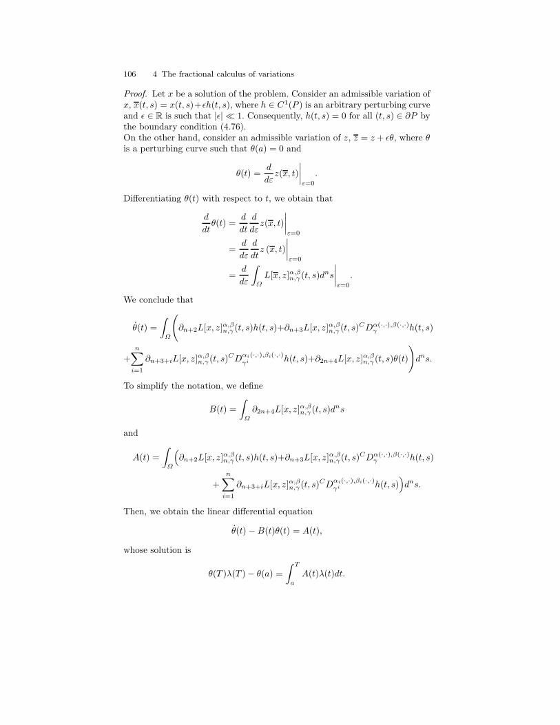
106 4 The fractional calculus of variations
Proof. Let x be a solution of the problem. Consider an admissible variation ofx, x(t, s) = x(t, s)+ǫh(t, s), where h ∈ C1(P ) is an arbitrary perturbing curveand ǫ ∈ R is such that |ǫ| ≪ 1. Consequently, h(t, s) = 0 for all (t, s) ∈ ∂P bythe boundary condition (4.76).On the other hand, consider an admissible variation of z, z = z + ǫθ, where θis a perturbing curve such that θ(a) = 0 and
θ(t) =d
dεz(x, t)
∣
∣
∣
∣
ε=0
.
Differentiating θ(t) with respect to t, we obtain that
d
dtθ(t) =
d
dt
d
dεz(x, t)
∣
∣
∣
∣
ε=0
=d
dε
d
dtz (x, t)
∣
∣
∣
∣
ε=0
=d
dε
∫
Ω
L[x, z]α,βn,γ (t, s)dns
∣
∣
∣
∣
ε=0
.
We conclude that
θ(t) =
∫
Ω
(
∂n+2L[x, z]α,βn,γ (t, s)h(t, s)+∂n+3L[x, z]
α,βn,γ (t, s)
CDα(·,·),β(·,·)γ h(t, s)
+
n∑
i=1
∂n+3+iL[x, z]α,βn,γ (t, s)
CDαi(·,·),βi(·,·)γi h(t, s)+∂2n+4L[x, z]
α,βn,γ (t, s)θ(t)
)
dns.
To simplify the notation, we define
B(t) =
∫
Ω
∂2n+4L[x, z]α,βn,γ (t, s)d
ns
and
A(t) =
∫
Ω
(
∂n+2L[x, z]α,βn,γ (t, s)h(t, s)+∂n+3L[x, z]
α,βn,γ (t, s)
CDα(·,·),β(·,·)γ h(t, s)
+
n∑
i=1
∂n+3+iL[x, z]α,βn,γ (t, s)
CDαi(·,·),βi(·,·)γi h(t, s)
)
dns.
Then, we obtain the linear differential equation
θ(t)−B(t)θ(t) = A(t),
whose solution is
θ(T )λ(T )− θ(a) =
∫ T
a
A(t)λ(t)dt.

4.7 Fractional variational Herglotz problem 107
Since θ(a) = θ(T ) = 0, we get
∫ T
a
A(t)λ(t)dt = 0. (4.80)
Considering only the second term in (4.80), we can write
∫ T
a
∫
Ω
λ(t)∂n+3L[x, z]α,βn,γ (t, s)
(
γ1CaD
α(·,·)t h(t, s) + γ2
Ct D
β(·,·)b h(t, s)
)
dnsdt
= γ1
∫ T
a
∫
Ω
λ(t)∂n+3L[x, z]α,βn,γ (t, s)
CaD
α(·,·)t h(t, s)dnsdt
+ γ2
[
∫ b
a
∫
Ω
λ(t)∂n+3L[x, z]α,βn,γ (t, s)
Ct D
β(·,·)b h(t, s)dnsdt
−∫ b
T
∫
Ω
λ(t)∂n+3L[x, z]α,βn,γ (t, s)
Ct D
β(·,·)b h(t, s)dnsdt
]
.
Let γ = (γ2, γ1). Integrating by parts (cf. Theorem 13), and since h(a, s) =
h(b, s) = 0 for all s ∈ Ω, we obtain the following expression:
∫ T
a
∫
Ω
h(t, s)Dβ(·,·),α(·,·)γ
(
λ(t)∂n+3L[x, z]α,βn,γ (t, s)
)
dnsdt
+ γ2
∫ b
T
∫
Ω
h(t, s)[
aDβ(·,·)t
(
λ(t)∂n+3L[x, z]α,βn,γ (t, s)
)
− TDβ(·,·)t
(
λ(t)∂n+3L[x, z]α,βn,γ (t, s)
)
]
dnsdt
+
∫
Ω
h(T, s)[
γ1tI1−α(·,·)T
(
λ(t)∂n+3L[x, z]α,βn,γ (t, s)
)
−γ2 T I1−β(·,·)t
(
λ(t)∂n+3L[x, z]α,βn,γ (t, s)
)
dns]
t=T.
Doing similarly for the (i + 2)th term in (4.80), with i = 1, . . . , n, lettingγi = (γi
2, γi1), and since h(t, ai) = h(t, bi) = 0 for all t ∈ [a, b], we obtain
∫ T
a
∫
Ω
λ(t)∂n+3+iL[x, z]α,βn,γ (t, s)
(
γi1CaiDαi(·,·)
si h(t, s) + γi2CsiD
βi(·,·)bi
h(t, s))
dnsdt
=
∫ T
a
∫
Ω
h(t, s)Dβi(·,·),αi(·,·)
γi
(
λ(t)∂n+3+iL[x, z]α,βn,γ (t, s)
)
dnsdt.
Substituting these relations into (4.80), we deduce that

108 4 The fractional calculus of variations
∫ T
a
∫
Ω
h(t, s)[
∂n+2L[x, z]α,βn,γ (t, s)λ(t) +D
β(·,·),α(·,·)γ
(
λ(t)∂n+3L[x, z]α,βn,γ (t, s)
)
+n∑
i=1
Dβi(·,·),αi(·,·)
γi
(
λ(t)∂n+3+iL[x, z]α,βn,γ (t, s)
)
dnsdt
+ γ2
∫ b
T
∫
Ω
h(t, s)[
aDβ(·,·)t
(
λ(t)∂n+3L[x, z]α,βn,γ (t, s)
)
−TDβ(·,·)t
(
λ(t)∂n+3L[x, z]α,βn,γ (t, s)
)
]
dnsdt
+
∫
Ω
h(T, s)[
γ1tI1−α(·,·)T
(
λ(t)∂n+3L[x, z]α,βn,γ (t, s)
)
−γ2 T I1−β(·,·)t
(
λ(t)∂n+3L[x, z]α,βn,γ (t, s)
)
dns]
t=T.
For appropriate choices with respect to h, we get the Euler–Lagrange equa-tions (4.77)–(4.78) and the transversality condition (4.79).
4.7.3 Examples
We present three examples, with and without the dependence on z.
Example 4.1. Consider
z(t) =(
CDα(·,·),β(·,·)γ x(t)
)2
+ z(t) + t2 − 1, t ∈ [0, 3],
x(0) = 1, z(0) = 0.(4.81)
In this case, λ(t) = exp(−t). The necessary optimality conditions (4.71)–(4.72)of Theorem 57 hold for x(t) ≡ 1. If we replace x by x in (4.81), we obtain
z(t)− z(t) = t2 − 1, t ∈ [0, 3],
z(0) = 0,
whose solution isz(t) = exp(t)− (t+ 1)2. (4.82)
The last transversality condition of Theorem 57 asserts that
L[x, z]α,βγ (T ) = 0 ⇔ exp(T )− 2T − 2 = 0,
whose solution is approximately
T ≈ 1.67835.
We remark that z (4.82) actually attains a minimum value at this point (seeFigure 4.1, (a)):
z(1.67835) ≈ −1.81685.

4.7 Fractional variational Herglotz problem 109
Example 4.2. Consider now
z(t) = (t− 1)(
x2(t) + z2(t) + 1)
, t ∈ [0, 3],
x(0) = 0, z(0) = 0.(4.83)
Since the first Euler–Lagrange equation (4.71) reads
(t− 1)x(t) = 0, ∀t ∈ [0, T ],
we see that x(t) ≡ 0 is a solution of this equation. The second transversalitycondition of (4.73) asserts that, at t = T , we must have
L[x, z]α,βγ (t) = 0,
that is,(t− 1)(z2(t) + 1) = 0,
and so T = 1 is a solution for this equation. Substituting x by x in (4.83), weget
z(t) = (t− 1)(z2(t) + 1), t ∈ [0, 3],
z(0) = 0.
The solution to this Cauchy problem is the function
z(t) = tan
(
t2
2− t
)
,
(see Figure 4.1, (b)) and the minimum value is
z(1) = tan
(
−1
2
)
.
Example 4.3. For our last example, consider
z(t) =(
CDα(·,·),β(·,·)γ x(t) − f(t)
)2
+ t2 − 1, t ∈ [0, 3],
x(0) = 0, z(0) = 0,(4.84)
where
f(t) :=t1−α(t)
2Γ (2− α(t))− (3− t)1−β(t)
2Γ (2− β(t)).
In this case, λ(t) ≡ 1. We intend to find a pair (x, z), satisfying all the con-ditions in (4.84), for which z(T ) attains a minimum value. It is easy to verifythat x(t) = t and T = 1 satisfy the necessary conditions given by Theorem57. Replacing x by x in (4.84), we get a Cauchy problem of form
z(t) = t2 − 1, t ∈ [0, 3],
z(0) = 0,

110 4 The fractional calculus of variations
whose solution is
z(t) =t3
3− t.
Observe that this function attains a minimum value at T = 1, which is z(1) =−2/3 (Figure 4.1, (c)).
(a) Extremal z of Example 4.1. (b) Extremal z of Example 4.2.
(c) Extremal z of Example 4.3.
Fig. 4.1. Graphics of function z(x, t).
References
Almeida R (2016) Fractional variational problems depending on indefiniteintegrals and with delay. Bull. Malays. Math. Sci. Soc. 39(4):1515–1528arXiv:1512.06752

References 111
Almeida R, Malinowska AB (2014) Fractional variational principle of Herglotz.Discrete Contin. Dyn. Syst. Ser. B 19(8):2367–2381
Baleanu D, Maaraba T, Jarad F (2008) Fractional variational principles withdelay. J. Phys. A 41(31):315403, 8 pp
Caputo MC, Torres DFM (2015) Duality for the left and right fractionalderivatives. Signal Process. 107:265–271 arXiv:1409.5319
Daftardar–Gejji V, Sukale Y, Bhalekar S (2015) Solving fractional delay dif-ferential equations: A new approach. Fract. Calc. Appl. Anal. 16:400–418
Deng W, Li C, Lu J (2007) Stability analysis of linear fractional differentialsystem with multiple time delays. Nonlinear Dynam. 48(4):409–416
Georgieva B, Guenther RB (2002) First Noether-type theorem for the gen-eralized variational principle of Herglotz. Topol. Methods Nonlinear Anal.20(2):261–273
Georgieva B, Guenther RB, Bodurov T (2003) Generalized variational princi-ple of Herglotz for several independent variables. J. Math. Phys. 44(9):3911–3927
Guenther RB, Gottsch JA, Kramer DB (1996) The Herglotz algorithm forconstructing canonical transformations. SIAM Rev. 38(2):287–293
Guenther RB, Guenther CM, Gottsch JA (1996) The Herglotz Lectures onContact Transformations and Hamiltonian Systems. Lecture Notes in Non-linear Analysis, Vol. 1, Juliusz Schauder Center for Nonlinear Studies,Nicholas Copernicus University, Torun
Herglotz G (1930) Beruhrungstransformationen, Lectures at the University ofGottingen, Gottingen
Jarad F, Abdeljawad T, Baleanu D (2010) Fractional variational principleswith delay within Caputo derivatives. Rep. Math. Phys. 65(1):17–28
Lazarevic MP, Spasic AM (2009) Finite-time stability analysis of fractional or-der time-delay systems: Gronwall’s approach. Math. Comput. Model. 49(3–4):475–481
Linge S, Langtangen HP (2016) Programming for Computations—MATLAB/Octave. A Gentle Introduction to Numerical Simulations withMATLAB/Octave. Springer, Cham
Machado JAT (2011) Time-delay and fractional derivatives. Adv. DifferenceEqu. Vol 2011:934094, 12 pp
Malinowska AB, Odzijewicz T, Torres DFM (2015) Advanced Methods in theFractional Calculus of Variations. Springer Briefs in Applied Sciences andTechnology, Springer, Cham
Santos SPS, Martins N, Torres DFM (2014) Higher-order variational problemsof Herglotz type. Vietnam J. Math. 42(4):409–419 arXiv:1309.6518
Santos SPS, Martins N, Torres DFM (2015a) Variational problems of Her-glotz type with time delay: DuBois-Reymond condition and Noether’s firsttheorem. Discrete Contin. Dyn. Syst. 35(9):4593–4610 arXiv:1501.04873
Santos SPS, Martins N, Torres DFM (2015b) An optimal control approach toHerglotz variational problems. In Optimization in the Natural Sciences (eds.

112 4 The fractional calculus of variations
A. Plakhov, T. Tchemisova and A. Freitas), Communications in Computerand Information Science, Vol. 499, Springer:107–117 arXiv:1412.0433
Tavares D, Almeida R, Torres DFM (2015) Optimality conditions for frac-tional variational problems with dependence on a combined Caputo deriva-tive of variable order. Optimization 64(6):1381–1391 arXiv:1501.02082
Tavares D, Almeida R, Torres DFM (2017) Constrained fractional variationalproblems of variable order. IEEE/CAA Journal Automatica Sinica 4(1):80–88 arXiv:1606.07512
Tavares D, Almeida R, Torres DFM (2018a) Fractional Herglotz variationalproblem of variable order. Discrete Contin. Dyn. Syst. Ser. S 11(1):143–154.arXiv:1703.09104
Tavares D, Almeida R, Torres DFM (2018b) Combined fractional variationalproblems of variable order and some computational aspects. J. Comput.Appl. Math. 339:374–388. arXiv:1704.06486
Trefethen LN (2013) Approximation Theory and Approximation Practice.Society for Industrial and Applied Mathematics
van Brunt B (2004) The Calculus of Variations. Universitext, Springer, NewYork
Wang H, Yu Y, Wen G, Zhang S (2015) Stability analysis of fractional orderneural networks with time delay. Neural Process. Lett. 42(2):479–500

Appendix
In this appendix, we use a specific MATLAB software, the package Chebfun, toobtain a few computational approximations for the main fractional operatorsin this book.
Chebfun is an open source software package that “aims to provide numer-ical computing with functions” in MATLAB (Linge and Langtangen, 2016).Chebfun overloads MATLAB’s discrete operations for matrices to analogouscontinuous operations for functions and operators (Trefethen, 2013). For themathematical underpinnings of Chebfun, we refer the reader to (Trefethen,2013). For the algorithmic backstory of Chebfun, we refer to (Driscoll, Hale and Trefethen,2014).
In what follows, we study some computational approximations of Riemann–Liouville fractional integrals, of Caputo fractional derivatives and conse-quently of the combined Caputo fractional derivative, all of them withvariable-order. We provide, also, the necessary Chebfun code for the variable-order fractional calculus.
To implement these operators, we need two auxiliary functions: the gammafunction Γ (Definition 1) and the beta function B (Definition 3). Bothfunctions are available in MATLAB through the commands gamma(t) andbeta(t,u), respectively.
A.1 Higher-order Riemann–Liouville fractional integrals
In this section, we discuss computational aspects to the higher-order Riemann–
Liouville fractional integrals of variable-order aIαn(·,·)t x(t) and tI
αn(·,·)b x(t).
Considering the Definition 34 of higher-order Riemann–Liouville fractionalintegrals, we implemented in Chebfun two functions leftFi(x,alpha,a) andrightFI(x,alpha,b) that approximate, respectively, the Riemann–Liouville
fractional integrals aIαn(·,·)t x(t) and tI
αn(·,·)b x(t), through the following Cheb-
fun/MATLAB code.

114 APPENDIX
function r = leftFI(x,alpha,a)
g = @(t,tau) x(tau)./(gamma(alpha(t,tau)).*(t-tau).^(1-alpha(t,tau)));
r = @(t) sum(chebfun(@(tau) g(t,tau),[a t],’splitting’,’on’),[a t]);
end
and
function r = rightFI(x,alpha,b)
g = @(t,tau) x(tau)./(gamma(alpha(tau,t)).*(tau-t).^(1-alpha(tau,t)));
r = @(t) sum(chebfun(@(tau) g(t,tau),[t b],’splitting’,’on’),[t b]);
end
With these two functions, we illustrate their use in the following exam-ple, where we determine computacional approximations for Riemann–Liouvillefractional integrals of a special power function.
Example 4.4. Let α(t, τ) = t2+τ2
4 and x(t) = t2 with t ∈ [0, 1]. In this case,
a = 0, b = 1 and n = 1. We have aIα(·,·)0.6 x(0.6) ≈ 0.2661 and 0.6I
α(·,·)b x(0.6) ≈
0.4619, obtained in MATLAB with our Chebfun functions as follows:
a = 0; b = 1; n = 1;
alpha = @(t,tau) (t.^2+tau.^2)/4;
x = chebfun(@(t) t.^2, [0,1]);
LFI = leftFI(x,alpha,a);
RFI = rightFI(x,alpha,b);
LFI(0.6)
ans = 0.2661
RFI(0.6)
ans = 0.4619
Other values for aIα(·,·)t x(t) and tI
α(·,·)b x(t) are plotted in Figure 4.2.
A.2 Higher-order Caputo fractional derivatives
In this section, considering the Definition 36, we implement in Chebfun twonew functions leftCaputo(x,alpha,a,n) and rightCaputo(x,alpha,b,n)
that approximate, respectively, the higher-order Caputo fractional derivatives
of variable-order CaD
αn(·,·)t x(t) and C
t Dαn(·,·)b x(t).
The following code implements the left operator (4.2):
function r = leftCaputo(x,alpha,a,n)
dx = diff(x,n);
g = @(t,tau) dx(tau)./(gamma(n-alpha(t,tau)).
*(t-tau).^(1+alpha(t,tau)-n));
r = @(t) sum(chebfun(@(tau) g(t,tau),[a t],’splitting’,’on’),[a t]);
end
Similarly, we define the right operator (4.3) with Chebfun in MATLAB asfollows:

115
0.1 0.2 0.3 0.4 0.5 0.6 0.7 0.8 0.90
0.1
0.2
0.3
0.4
0.5
0.6
0.7
0.8
0.9
Fig. 4.2. Riemann–Liouville fractional integrals of Example 4.4: x(t) = t2 in con-
tinuous line, left integral aIα(·,·)t x(t) with “−” style, and right integral tI
α(·,·)b x(t)
with “×−” style.
function r = rightCaputo(x,alpha,b,n)
dx = diff(x,n);
g = @(t,tau) dx(tau)./(gamma(n-alpha(tau,t)).
*(tau-t).^(1+alpha(tau,t)-n));
r = @(t)(-1).^n.* sum(chebfun(@(tau) g(t,tau),[t b],
’splitting’,’on’),[t b]);
end
We use the two functions leftCaputo and rightCaputo to determine apro-ximations for the Caputo fractional derivatives of a power function of the formx(t) = tγ .
Example 4.5. Let α(t, τ) = t2
2 and x(t) = t4 with t ∈ [0, 1]. In this case, a = 0,
b = 1 and n = 1. We have CaD
α(·,·)0.6 x(0.6) ≈ 0.1857 and C
0.6Dα(·,·)b x(0.6) ≈
−1.0385, obtained in MATLAB with our Chebfun functions as follows:
a = 0; b = 1; n = 1;
alpha = @(t,tau) t.^2/2;
x = chebfun(@(t) t.^4, [a b]);
LC = leftCaputo(x,alpha,a,n);
RC = rightCaputo(x,alpha,b,n);
LC(0.6)
ans = 0.1857
RC(0.6)

116 APPENDIX
ans = -1.0385
See Figure 4.3 for a plot with other values of CaD
α(·,·)t x(t) and C
t Dα(·,·)b x(t).
0.1 0.2 0.3 0.4 0.5 0.6 0.7 0.8 0.9-1.5
-1
-0.5
0
0.5
1
1.5
Fig. 4.3. Caputo fractional derivatives of Example 4.5: x(t) = t4 in continuous line,
left derivative Ca D
α(·,·)t x(t) with “−” style, and right derivative C
t Dα(·,·)b x(t) with
“×−” style.
Example 4.6. In Example 4.5, we have used the polynomial x(t) = t4. It isworth mentioning that our Chebfun implementation works well for functionsthat are not a polynomial. For example, let x(t) = et. In this case, we justneed to change
x = chebfun(@(t) t.^4, [a b]);
in Example 4.5 by
x = chebfun(@(t) exp(t), [a b]);
to obtain
LC(0.6)
ans = 0.9917
RC(0.6)
ans = -1.1398
See Figure 4.4 for a plot with other values of CaD
α(·,·)t x(t) and C
t Dα(·,·)b x(t).

117
0.1 0.2 0.3 0.4 0.5 0.6 0.7 0.8 0.9-1.5
-1
-0.5
0
0.5
1
1.5
2
2.5
Fig. 4.4. Caputo fractional derivatives of Example 4.6: x(t) = et in continuous line,
left derivative Ca D
α(·,·)t x(t) with “−” style, and right derivative C
t Dα(·,·)b x(t) with
“×−” style.
With Lemma 40 in Section 4.1 we can obtain, analytically, the higher-orderleft Caputo fractional derivative of a power function of the form x(t) = (t−a)γ .This allows us to show the effectiveness of our computational approach, thatis, the usefulness of polynomial interpolation in Chebyshev points in fractionalcalculus of variable-order. In Lemma 40, we assume that the fractional orderdepends only on the first variable: αn(t, τ) := αn(t), where αn : [a, b] →(n− 1, n) is a given function.
Example 4.7. Let us revisit Example 4.5 by choosing α(t, τ) = t2
2 and x(t) = t4
with t ∈ [0, 1]. Table 4.1 shows the approximated values obtained by our Cheb-fun function leftCaputo(x,alpha,a,n) and the exact values computed withthe formula given by Lemma 40. Table 4.1 was obtained using the followingMATLAB code:
format long
a = 0; b = 1; n = 1;
alpha = @(t,tau) t.^2/2;
x = chebfun(@(t) t.^4, [a b]);
exact = @(t) (gamma(5)./gamma(5-alpha(t))).*t.^(4-alpha(t));
approximation = leftCaputo(x,alpha,a,n);
for i = 1:9
t = 0.1*i;
E = exact(t);

118 APPENDIX
A = approximation(t);
error = E - A;
[t E A error]
end
t Exact Value Approximation Error
0.1 1.019223177296953e-04 1.019223177296974e-04 -2.046431600566390e-18
0.2 0.001702793965464 0.001702793965464 -2.168404344971009e-18
0.3 0.009148530806348 0.009148530806348 3.469446951953614e-18
0.4 0.031052290994593 0.031052290994592 9.089951014118469e-16
0.5 0.082132144921157 0.082132144921157 6.522560269672795e-16
0.6 0.185651036003120 0.185651036003112 7.938094626069869e-15
0.7 0.376408251363662 0.376408251357416 6.246059225389899e-12
0.8 0.704111480975332 0.704111480816562 1.587694420379648e-10
0.9 1.236753486749357 1.236753486514274 2.350835082154390e-10
Table 4.1. Exact values obtained by Lemma 40 for functions of Example 4.7 versuscomputational approximations obtained using the Chebfun code.
Computational experiments similar to those of Example 4.7, obtained bysubstituting Lemma 40 by Lemma 41 and our leftCaputo routine by therightCaputo one, reinforce the validity of our computational methods. Inthis case, we assume that the fractional order depends only on the secondvariable: αn(τ, t) := αn(t), where αn : [a, b] → (n− 1, n) is a given function.
A.3 Higher-order combined fractional Caputo derivative
The higher-order combined Caputo fractional derivative combines both leftand right Caputo fractional derivatives, that is, we make use of functionsleftCaputo(x,alpha,a,n)and rightCaputo(x,alpha,b,n)provided in Sec-tion A.1 to define Chebfun computational code for the higher-order combinedfractional Caputo derivative of variable-order:
function r = combinedCaputo(x,alpha,beta,gamma1,gamma2,a,b,n)
lc = leftCaputo(x,alpha,a,n);
rc = rightCaputo(x,beta,b,n);
r = @(t) gamma1 .* lc(t) + gamma2 .* rc(t);
end
Then we illustrate the behavior of the combined Caputo fractional deriva-tive of variable-order for different values of t ∈ (0, 1), using MATLAB.
Example 4.8. Let α(t, τ) = t2+τ2
4 , β(t, τ) = t+τ3 and x(t) = t, t ∈ [0, 1].
We have a = 0, b = 1 and n = 1. For γ = (γ1, γ2) = (0.8, 0.2), we haveCD
α(·,·),β(·,·)γ x(0.4) ≈ 0.7144:

References 119
a = 0; b = 1; n = 1;
alpha = @(t,tau) (t.^2 + tau.^2)/.4;
beta = @(t,tau) (t + tau)/3;
x = chebfun(@(t) t, [0 1]);
gamma1 = 0.8;
gamma2 = 0.2;
CC = combinedCaputo(x,alpha,beta,gamma1,gamma2,a,b,n);
CC(0.4)
ans = 0.7144
For other values of CDα(·,·),β(·,·)γn x(t), for different values of t ∈ (0, 1) and
γ = (γ1, γ2), see Figure 4.5 and Table 4.2.
0.1 0.15 0.2 0.25 0.3 0.35 0.4 0.45-0.8
-0.6
-0.4
-0.2
0
0.2
0.4
0.6
0.8
1
Fig. 4.5. Combined Caputo fractional derivative CDα(·,·),β(·,·)γ x(t) for α(·, ·), β(·, ·)
and x(t) of Example 4.8: continuous line for γ = (γ1, γ2) = (0.2, 0.8), “−” style forγ = (γ1, γ2) = (0.5, 0.5), and “×−” style for γ = (γ1, γ2) = (0.8, 0.2).
References
Driscoll TA, Hale N, Trefethen LN (2014) Chebfun Guide. Pafnuty Publica-tions, Oxford
Linge S, Langtangen HP (2016) Programming for Computations—MATLAB/Octave. A Gentle Introduction to Numerical Simulations withMATLAB/Octave. Springer, Cham

120 APPENDIX
t Case 1 Case 2 Case 3
0.4500 -0.5630 -0.3371 -0.1112
0.5000 -790.4972 -1.9752e+03 -3.1599e+03
0.5500 -3.5738e+06 -8.9345e+06 -1.4295e+07
0.6000 -2.0081e+10 -5.0201e+10 -8.0322e+10
0.6500 2.8464e+14 7.1160e+14 1.1386e+15
0.7000 4.8494e+19 1.2124e+20 1.9398e+20
0.7500 3.8006e+24 9.5015e+24 1.5202e+25
0.8000 -1.3648e+30 -3.4119e+30 -5.4591e+30
0.8500 -1.6912e+36 -4.2280e+36 -6.7648e+36
0.9000 5.5578e+41 1.3895e+42 2.2231e+42
0.9500 1.5258e+49 3.8145e+49 6.1033e+49
0.9900 1.8158e+54 4.5394e+54 7.2631e+54
Table 4.2. Combined Caputo fractional derivative CDα(·,·),β(·,·)γ x(t) for α(·, ·), β(·, ·)
and x(t) of Example 4.8. Case 1: γ = (γ1, γ2) = (0.2, 0.8); Case 2: γ = (γ1, γ2) =(0.5, 0.5); Case 3: γ = (γ1, γ2) = (0.8, 0.2).
Trefethen LN (2013) Approximation Theory and Approximation Practice.Society for Industrial and Applied Mathematics

Index
admissible trajectory, 22admissible variation, 23approximation error, 45, 49, 52, 53
beta function, 4, 41, 65, 113boundary conditions, 22, 24, 55, 58, 68,
69, 75, 83, 87, 92, 96, 101brachistochrone, 22
Caputo fractional derivativeleft, 7left (higher-order), 63, 64left (variable-order), 14partial left, 44partial right, 44right, 7right (higher-order), 63right (variable-order), 14several variables, 42
combined Caputo fractional derivativeclassical, 12higher-order, 66variable-order, 62
combined Riemann–Liouville fractionalderivative
higher-order, 65variable-order, 62
dual parameter set, 17
Euler–Lagrange equations, 23, 28, 30,69, 76, 83, 87, 92, 96, 102
expansion formulas, 45, 49, 51–53extremal, 24
first variation, 23
gamma function, 4, 113generalized fractional derivative
of Caputo, 15of Riemann–Liouville, 15
generalized fractional integralsof Riemann–Liouville, 14
Grunwald-Letnikov fractional deriva-tive, 9
Hadamard fractional derivativeleft, 9right, 9
Hadamard fractional integralleft, 6right, 6
holonomic constraint, 95, 96horizontal terminal line, 73
integration by partsCaputo fractional derivative of
higher-order, 66Caputo fractional derivatives, 16, 68Caputo fractional derivatives of
variable-order, 16fractional integrals of variable-order,
16Riemann–Liouville fractional
integrals, 16isoperimetric problem, 25, 86
Lagrange multiplier, 26

122 Index
Mittag-Leffler functionone parameter, 5two parameters, 5
psi function, 4
Riemann–Liouville fractional derivativeleft, 7left (higher-order), 63left (variable-order), 13right, 7right (higher-order), 63right (variable-order), 13
Riemann–Liouville fractional integralleft, 6left (higher-order), 63left (variable-order), 13right, 6right (higher-order), 63right (variable-order), 13
Riesz fractional derivative, 11Riesz fractional integral, 11Riesz–Caputo fractional derivative, 11
symmetric fractional derivative, 11
tautochrone problem, 2, 27terminal cost function, 69, 75, 87, 96terminal curve, 73time delay, 82transversality conditions, 24, 25, 29, 69,
72, 76, 81, 88, 91, 93, 97, 102, 105
variational fractional problem, 28, 29fundamental, 69higher-order, 75of Herglotz, 101with a holonomic constraint, 95with time delay, 83
vertical terminal line, 73