
The Value of Gradually Spreading Information
43
The Value of Diffusing Information Forthcoming in the Journal of Financial Economics Asaf Manela * August 6, 2013 Abstract How does the speed by which information diffuses affect its value to a stock market investor? In a structural model solved in closed-form, this speed has two opposing effects on the empiri- cally dominant term of the value of information. Faster-diffusing information means quicker and less noisy profits, but also increases competing informed trading, impounding more information into prices and eroding profits. Structural empirical analysis of stock market reaction to drug approvals using media coverage as a proxy for the transmission rate of information finds that the value of information is hump-shaped in its future transmission rate. Moreover, the estimated amount of noise trading is small. JEL Classification: G12, D82, D83 Keywords: value of information, information choice, information diffusion, percolation, learning, media coverage, drug approvals * Washington University in St. Louis, Olin Business School, [email protected]. This paper is based on my University of Chicago Dissertation. I thank Pietro Veronesi, Douglas Diamond, John Heaton and Lubos Pastor for their guidance. This paper has benefited from helpful comments and suggestions from an anonymous referee, Tal Barak-Manela, Zahi Ben-David, Phil Dybvig, Andrea Frazzini, Matthew Gentzkow, Michael Gofman, Ohad Kadan, Roni Kisin, Alan Moreira, Toby Moskowitz, Alexi Savov, David Solomon, Paul Tetlock, Anjan Thakor, Luigi Zingales, and seminar participants at ASU, Boston College, Chicago, Hebrew U, LBS, Maryland, Tel-Aviv and Wash U, the WFA meeting in Santa Fe, the Econometric Society meeting in Rio de Janeiro, and the LBS Trans-Atlantic Doctoral Conference. Remaining errors are my own.
Transcript of The Value of Gradually Spreading Information

The Value of Diffusing Information
Forthcoming in the Journal of Financial Economics
Asaf Manela∗
August 6, 2013
Abstract
How does the speed by which information diffuses affect its value to a stock market investor?
In a structural model solved in closed-form, this speed has two opposing effects on the empiri-
cally dominant term of the value of information. Faster-diffusing information means quicker and
less noisy profits, but also increases competing informed trading, impounding more information
into prices and eroding profits. Structural empirical analysis of stock market reaction to drug
approvals using media coverage as a proxy for the transmission rate of information finds that the
value of information is hump-shaped in its future transmission rate. Moreover, the estimated
amount of noise trading is small.
JEL Classification: G12, D82, D83
Keywords: value of information, information choice, information diffusion, percolation, learning,
media coverage, drug approvals
∗Washington University in St. Louis, Olin Business School, [email protected]. This paper is based on myUniversity of Chicago Dissertation. I thank Pietro Veronesi, Douglas Diamond, John Heaton and Lubos Pastor fortheir guidance. This paper has benefited from helpful comments and suggestions from an anonymous referee, TalBarak-Manela, Zahi Ben-David, Phil Dybvig, Andrea Frazzini, Matthew Gentzkow, Michael Gofman, Ohad Kadan,Roni Kisin, Alan Moreira, Toby Moskowitz, Alexi Savov, David Solomon, Paul Tetlock, Anjan Thakor, Luigi Zingales,and seminar participants at ASU, Boston College, Chicago, Hebrew U, LBS, Maryland, Tel-Aviv and Wash U, theWFA meeting in Santa Fe, the Econometric Society meeting in Rio de Janeiro, and the LBS Trans-Atlantic DoctoralConference. Remaining errors are my own.
1 Introduction
How does the speed by which information diffuses affect its value to a stock market investor?
Consider two drugs: Viagra treats erectile dysfunction while Allegra fights nasal allergies. Both
drugs, if approved by the FDA, would generate similar revenues to their publicly traded developers.
When Viagra is approved, news of the approval diffuses fast because it makes for good conversation,
while news of Allegra’s approval travels slower. As an investor, would you pay more today to know
that Viagra or Allegra will be approved tomorrow?
Theoretically, I show that faster-diffusing information can be more or less valuable. Intuitively,
faster-diffusing information translates into a quicker realization of profits that are subject to less
noise. However, competing informed agents trade more aggressively on faster-diffusing information,
impounding more information into prices, thus decreasing the returns to informational trading.
Empirically, the value of drug approval information turns out to be hump-shaped in its diffusion
speed. Therefore the most valuable information diffuses at a moderate speed.
I construct an asset pricing model where the transmission rate of information determines equi-
librium asset prices and volume. The model is a four-period noisy rational expectations model, a la
Grossman and Stiglitz (1980), with asymmetric information about a risky asset that pays-off in the
post-announcement period. Information diffuses through a large population of risk-averse agents.
The transmission rate controls the probability that uninformed agents in the pre-announcement
period become informed for free in the announcement period. Pre-announcement, agents make
their endogenous information choice taking into account its future diffusion, through both direct
communication, and indirect learning from prices.1
The main theoretical result provides a closed-form expression for the value of information given
the transmission rate that has eluded previous studies of similar settings (Hirshleifer, Subrah-
manyam, and Titman, 1994; Holden and Subrahmanyam, 2002). It is the sum of three terms. The
first, and empirically dominant term, is positive and increasing in the intertemporal decline in unin-
1Money managers do in fact spread and exploit information over their social networks. Shiller and Pound (1989)provides survey evidence that direct interpersonal communication is important in investment decisions, and thatinvestor interest in specific stocks spreads like an epidemic. Hong, Kubik, and Stein (2005) provide further evidencethat mutual fund managers spread information directly, through word-of-mouth communication. Furthermore, Cohen,Frazzini, and Malloy (2008) find that portfolio managers gain an informational advantage through education networks,and that their returns from this channel are concentrated around corporate news announcements. Consistent with theStein (2009) model of truthful exchanges of information between competitors, Gray (2010) finds that skilled investorsshare their profitable ideas with their competition.
2

formed agents’ uncertainty. The transmission rate has two contrasting effects on this term: The first
and more intuitive effect is that informational gains realized earlier are better than those realized
only in the future that are subject to additional shocks. However, a second effect of this potential
gain is that informed agents trade more aggressively, which makes pre-announcement prices more
informative. The resulting reduction in pre-announcement uncertainty reduces the intertemporal
decline in uncertainty and lowers the equilibrium value of information.2
The second term of the value of information is positive as well and has to do with the intertem-
poral decline in uncertainty of the informed relative to this decline by the uninformed. The third
term is negative and represents the extent of information spillover to uninformed agents who do
not pay for the signal. In contemporaneous work, Han and Yang (forthcoming) study information
acquisition and market efficiency in a one-period model with information spillovers over networks.
In their model only this third term survives, which explains why they find that the value of infor-
mation is monotonically decreasing in its speed. The relative contribution of each of these terms
to the total value depends on the parameters of the model, mainly the prior variances of the noisy
supply and of the terminal payoff, and remains an empirical question, which I turn to next.
I estimate the parameters of the model and the magnitudes of the three terms of the value of
information in a panel of FDA drug approvals, using media coverage as a proxy for the approval-
specific transmission rate of information. Structural estimation reveals that the gradual information
diffusion model quantitatively matches well many empirical moments of stock returns and volume
around drug approvals. An open question about noisy rational expectations models is how much
noise is keeping equilibrium prices from revealing the signal to the uninformed. A requirement
of too much noise would question the validity of this theoretical assumption. Encouragingly, I
estimate that non-informational supply shocks (noise) have a standard deviation of 1% of the total
supply of the stock. Thus the model requires only a small amount of non-informational trading to
prevent prices from fully revealing the news.
Perhaps surprisingly, my main empirical finding is that the value of information is hump-shaped
in the transmission rate of information of the fitted model and stems entirely from the first term,
i.e. from its effect on the intertemporal decline in uninformed agents’ uncertainty. This result
2Note that this second effect happens holding the early informed fraction fixed. Unlike in Grossman-Stiglitz wherestrategic substitutability in information choice results from endogenous price informativeness, here price informative-ness affects the value of information through the aggressiveness of the same informed agents.
3

means that all else equal, the most valuable information to have early, diffuses at a moderate
rate later on. Furthermore, I find that the endogenous information choice feature of the model is
crucial to match the magnitude of the negative covariation between the transmission rate and post-
approval returns. In information market equilibrium, uninteresting news that propagates slowly
is not pursued by anyone before the official announcement, because the fixed cost of information
is prohibitively high. Faster-diffusing information is purchased at a higher rate, while the fastest
diffusing news is somewhat less valuable. This unique feature of the model accentuates the covari-
ation between transmission rates and the demand for the risky asset by influencing the extensive
margin of information acquisition by the population as a whole.
My model builds on foundations laid by previous asset pricing theories with sequential infor-
mation arrival. Hirshleifer, Subrahmanyam, and Titman (1994) randomly assigns the informed
population into early and late informed groups. In a similar setting, Holden and Subrahmanyam
(2002) allow agents to purchase information in any of two periods of their model and investigate
the serial correlation of stock returns and trade volume. I improve on their numerical work by
characterizing the value of information in an intuitive closed-form expression. I further consider
the problem of uninformed investors that randomly become informed in the future. Hong and Stein
(1999) provides a behavioral model with information diffusion across a population of differentially
and symmetrically informed “newswatchers.” The rational part of their model is closely related
to my model. I extend their work with optimal learning from prices, information acquisition, and
information asymmetry in the sense that different agents have different precision of information.
Information acquisition is also central in Veldkamp (2006) which studies media frenzies in emerg-
ing markets and uses the aggregate number of articles that reference an emerging market as a
proxy for the cost of information in different environments. By contrast, the focus in my paper
is on specific anticipated news and the market reactions they induce. Other recent work on in-
formation acquisition studies large price movements (Barlevy and Veronesi, 2000; Dow, Goldstein,
and Guembel, 2011; Mele and Sangiorgi, 2011; Garcıa and Strobl, 2011), portfolio choice (Per-
ess, 2004; Van Nieuwerburgh and Veldkamp, 2010), mutual funds behavior (Garcia and Vanden,
2009; Kacperczyk, Nieuwerburgh, and Veldkamp, 2012), the home bias puzzle (Nieuwerburgh and
Veldkamp, 2009), and bank runs (He and Manela, 2012). For a good review of this literature see
Veldkamp (2011).
4
More broadly, this paper relates to a literature on the diffusion of information in markets.
Duffie and Manso (2007) and subsequently Duffie, Malamud, and Manso (2009, 2010) study the
“percolation” of information through agents’ encounters in large but decentralized markets. Hong,
Hong, and Ungureanu (2011) study a dynamic model of opinions, prices and volume based on word-
of-mouth communication. They allow for intricate information diffusion dynamics at the cost of a
simplified asset pricing framework in which agents agree to disagree and behave myopically. Colla
and Mele (2010) and Ozsoylev and Walden (2011) show that social communication improves price
informativeness in an exogenous information environment. I embed a simpler diffusion technology
in a centralized market with Bayesian learning from prices, and focus on the value of information
in this environment.3
This is one of the first papers to empirically test the implications of asymmetric information
asset pricing models. Kelly and Ljungqvist (2012) tests several predictions of the Easley and O’hara
(2004) model by exploiting various natural experiments involving shocks to research coverage by
sell-side equity analysts. Quantitative related work by Cho and Krishnan (2000) estimates a small
amount of noise in a Hellwig (1980) dispersed information model. Savov (2012) calibrates a dynamic
dispersed information model to study mutual fund performance. The approach here of focusing on
a particular anticipated news release, namely drug approvals, using media coverage as a proxy for
the transmission rate of information is novel.
The paper proceeds as follows. Section 2 describes the model. Section 3 describes the drug
approvals sample. Section 4 then proceeds with structural estimation. Section 5 concludes.
2 Model
I construct an asset pricing model with the necessary features for the discussion and empirical
analysis, and describe its main predictions. The model extends the Grossman and Stiglitz (1980)
framework to a three-trading period economy with a fraction of informed investors that evolves
deterministically over time and is known by all market participants. The model has four periods
labeled t = 0, 1, 2, 3, where the first three involve trade, and all uncertainty is revealed in period 3.
3Also related is Daley and Green (2012) which studies market outcomes when information (or news) about anasset’s type is gradually revealed to all potential buyers simultaneously when a seller knows its true value, as well asa literature on the supply of financial information which I abstract from (Admati and Pfleiderer, 1986, 1988; Fishmanand Hagerty, 1995; Garcıa and Sangiorgi, 2011).
5

Figure 1: Informational Types over Time
t = 0 1 2 3
Informed Early at Time 1 (II )
Informed Late at Time 2 (UI )
Uninformed until Time 3 (UU )
I1
1−I1
Γ(I1,δ)
1− Γ(I1, δ)
R1 R2
OfficialAnnouncement
R3
2.1 Preferences, Endowments and Tradable Assets
Agents can trade an elastically supplied risk-free asset with constant gross return R per period
that is exogenously given. The second asset offers a risky payoff u = θ + ε in period 3, where
θ ∼ N (µ0,1τ0
) and ε ∼ N (0, 1η ) are independent shocks and the precisions τ0 and η are positive.
Agents enter period 0 with identical preferences and endowments. Agents of type i maximize their
constant absolute risk aversion (CARA) utility over terminal wealth
V i0 (W i
0) = maxqit2
t=0
E[−e−
1φW i
3 |F i0],
by choosing the amount of shares qt, while satisfying the law of motion of their stochastic wealth
W it+1 = RW i
t + qitQt+1, where Qt+1 ≡ pt+1 − Rpt is the return to a zero-investment portfolio long
one share of the risky asset.4 The initial endowments, W0, are given and F it is the information set
of agent i described next.
2.2 Diffusing Information
At the initial period 0, all agents are identical and choose not to trade at the market-clearing price.
A signal θ is revealed in period 1 to a fraction I1 ∈ [0, 1] of the population, which choose to pay a
4The role of risk aversion here is to prevent informed agents from fully revealing their information through extremedemand for the risky asset. Alternative ways to generate the same phenomena include market power by informed(Kyle, 1985) or borrowing constraints (Barlevy and Veronesi, 2000).
6

fixed cost c for this information. This fraction is determined in equilibrium. Information diffuses
deterministically between periods 1 and 2 as follows:
I2 − I1 = Γ(I1; δ)(1− I1). (1)
The incidence probability Γ(I; δ) is the probability that an uninformed agent at time 1 will become
informed at time 2. It potentially depends on the fraction informed to allow for word-of-mouth
transmission of information. The incidence probability is increasing in the transmission rate (∂Γ∂δ >
0) so that, all else equal, the uninformed are more likely to receive more interesting news, for which
the transmission rate is higher. The payoff u is revealed in period 3 and all agents know It and its
law of motion.
Figure 1 illustrates the time-line of information diffusion. Agents of type II observe the signal.
They remain informed for the rest of time. Uninformed agents at time 1 become informed next
period with probability Γ(I1; δ). This key addition to the canonical model adds a new, third type
of agent that affects the dynamics of asset prices and the volume of trade. Agents of type UI are
uninformed agents that become informed via direct information transmission. The rest, agents of
type UU , remain uninformed until time 3. The three return periods of the model are meant to
capture the periods before, on, and after an official announcement of news such as a drug approval
as illustrated at the top.
All agents know the structure of the world and its parameters, including the transmission rate,
and observe current prices, as well as their entire history. Thus an informed agent’s information
set at time t is FIt =pt, It, θ
, whereas that of an uninformed agent at time t is FUt =
pt, It
,
where the superscript t denotes the entire history of the variable.
2.3 Noise
To prevent prices from fully revealing all information, I allow for noise in the supply of the risky
asset. This noise traditionally has several interpretations, such as liquidity shocks (Wang, 1994),
or allocational price changes (Grossman, 1995). How much noise is required to perform this task
is an open question that I tackle in Section 4 below.
Let x denote the mean supply of the risky asset, which is augmented in every trading period
7

by i.i.d noise xt ∼ N (0, 1ξ ) for t = 1, 2 with strictly positive precision ξ. Thus the risky asset
market-clearing condition is
ItqIt + (1− It)qUt = x+ xt t = 0, 1, 2, (2)
where x0 = 0, qIt is the risky asset holdings of an informed agent leaving period t and qUt is that of
an uninformed agent. In general, type UI demand would enter separately in (2), but since wealth
does not enter the optimal demand functions with these preferences, agents of type UI will behave
just like the initially informed of type II going forward.
2.4 A Noisy Linear Rational Expectations Equilibrium
The assumed structure admits a noisy rational expectations equilibrium with prices that are linear
in the state as made formal by the following proposition:
Proposition 1 (Existence of Equilibrium). There exists a REE with prices that are linear in the
state. Specifically, prices take the form:
pt = at + bt∆t + ctxt t = 1, 2 (3)
p0 = a0,
where ∆t ≡ θ − µt is the prediction error of the uninformed and the coefficients at, bt, and ct are
measurable with respect to the uninformed information set at time t− 1.
The coefficient at is the uninformed agent’s expectation of the price next period. It is composed
of the discounted present value of the expected payoff minus a risk premium. The coefficient bt
measures the price sensitivity to the uninformed agent’s error at time t. It is non-negative and
grows larger the more informed agents there are and the less uncertainty there is in the market
about the return going into the next period. Finally, ct < 0 is the price sensitivity to supply shocks.
The ratio between bt and ct determines the informativeness of the equilibrium price.
The proof of Proposition 1 proceeds in the usual “guess and verify” manner and appears in the
appendix where I obtain closed-form expressions for all variables in the model. The solution of the
model comes down to finding the root of a cubic polynomial. As such, it admits a single real solution
8

as long as its discriminant is negative. At least one real solution must exist by the intermediate
value theorem, establishing the existence of equilibrium. The condition on the discriminant implies
the following condition for uniqueness of the equilibrium in the linear class:
Proposition 2 (Uniqueness of Equilibrium). Suppose
4(γ3 + ξ2ζ4ω
)> ξζ2
(γ2 + 18γω − 27ω2
),
where ζ = φI1(η + η2I2ξφ
2), γ = η2I2ξφ2 + η + τ0 and ω = η2I2
2ξφ2 + η + τ0.
Then the equilibrium is unique in the linear class.
2.5 Learning from Equilibrium Prices
Uninformed agents are Bayesian and form rational expectations based on all of their available in-
formation, which in this case is restricted to the history of market clearing prices. The linearity of
prices, together with the normality of the noise and the prior on the signal θ, imply a normal poste-
rior distribution with a mean that is linear in prices and a precision that increases deterministically
over time as summarized by the following lemma:
Lemma 1 (Learning from Prices). Uninformed agent’s beliefs evolve:
EUt+1[θ] ≡ µt+1 = µt + kt+1(pt+1 − at+1) (4)
ΨUt+1[θ] ≡ τt+1 = τt + ξβ2
t+1
for t = 0, 1 with (µ0, τ0) given and where kt+1 ≡ ξbt+1τtc2
t+1and βt+1 ≡ bt+1
ct+1.
For notational brevity, Eit [·] denotes the expectation operator conditional on agent i’s informa-
tion set at time t. Similarly, Ψit[·] denotes the conditional precision operator, defined as the inverse
of the corresponding variance V arit[·]. Given their information of the signal, informed agents can
perfectly infer the supply shock. Their expectation of the payoff u is just θ, which they observe,
and its precision conditional on the signal, η, is constant. Note that nothing can be learned from
period 0 prices so no updating occurs.
Having characterized the existence and uniqueness of equilibrium, and the learning dynamics
9

when the information structure is given, I next turn to analysis of the market for information and
endogenize this structure.
2.6 Information Choice
Agents at time 1 must choose whether to purchase the signal θ at the exogenously given cost c. The
value of information v is the amount of wealth an uninformed agent is willing to pay to become
informed, such that he is indifferent between purchasing the signal or not. Therefore, v is such
that EU1
[V U
1 (W1;µ1)]
= EU1
[V I
1 (W1 − v; ∆1, x1)]
holds. Solving this equation for the value of
information as a function of the informed fraction yields the following result:
Proposition 3 (Value of Information). The value of information v given an initial fraction in-
formed I1 and transmission rate δ is
v (I1; δ) = φ
R2
12 log Ωv (I1; δ) + 1
2 log ΩI1 (I1; δ)
ΩU1 (I1; δ)
+ log[Γ (I1; δ)
√τ2τ2+η
+ (1− Γ (I1; δ))]
,(5)
where Ωv (I1; δ) = τ2+ητ1
and Ωi1 (I1; δ) = 1 + Ψi2[Q3](ρi1)2
Ψi1[Q2] for i ∈ U, I.
The first term of the value of information is positive and increasing in the intertemporal growth
rate of uninformed agents’ precision about returns. The steeper this increase is, the more valuable
the information. The transmission rate has two contrasting effects on this term. The first and more
intuitive effect is that informational gains realized earlier are better than those realized only in the
future and are subject to additional shocks. However, a second effect of this potential gain is that
informed agents trade more aggressively, which makes p1 more informative. The resulting increase
in τ1 reduces the intertemporal precision growth and lowers the equilibrium value of information.
The second term is positive as well and has to do with the intertemporal increase in precision of
the informed relative to this increase by the uninformed. The third term is negative and represents
the extent of information spillover to uninformed agents who do not pay for the signal. Intuitively,
an increase in the probability that an uninformed agent becomes informed next period, Γ (I1; δ),
decreases the value of information to those who purchase the signal because of the spillover effect.
The relative contribution of each of these terms depends on the parameters of the model, but
mainly on the precisions ξ, τ0 and η. For example, the third term will be more negative when η is
10
high relative to τ2. This means informational spillovers are more important when the variance of
the signal θ is large compared with the variance of ε. In Section 4, I estimate these parameters and
the relative magnitudes of the three terms.
In equilibrium, the fraction of informed agents, I∗1 , is such that agents are indifferent between
purchasing the signal or not. Equivalently, the equilibrium value of information v(I∗1 ; δ) equals
the cost of information c. Although the spillover effect works in the same direction as strategic
information substitutability, a range of I1 close to zero exists such that strategic complementarity
arises. That is, an increase in the cost of information will result in increased demand for informa-
tion. Therefore, with endogenous information choice multiple equilibria can arise depending on the
parameters. The empirical work below selects the only stable equilibrium in such cases. I discuss
the market for information further in Section 4.5.
3 Drug Approvals
The model described above yields predictions about observables such as returns and trade volume
and their response to variation in the transmission rate of information. What remains is finding a
suitable empirical environment to estimate its parameters.
I study a panel of new drug approvals by the U.S. Food and Drug Administration. I examine
a short time series of prices, volume, and media coverage around each approval. Times 0, 1, and
2 in the model correspond to the beginning of the pre-approval, approval, and post-approval event
windows, respectively. Thus the informed fraction at time 1 trades on information that has not yet
been publicly disclosed. The informed at time 2 include investors that receive the news directly
from centralized news outlets or alternatively by word-of-mouth from the informed at time 1.
It is important to note that there is no blunt distinction here between information that is public
vs. private, but rather there are only publicity shades of gray. Even if the drug sponsoring firm
issues a press release, this information is unlikely to reach 100% of the population. Of course,
information that reaches a large enough audience has a practically equal effect on prices as fully
public information, but this effect is within the model (high It) and therefore there is no need for
a binary distinction between public and private information.
I use media coverage as a proxy for the transmission rate of information. Specifically, I calculate
11

media exposure for each approval as the sum of all news articles that report the approval on the
official approval day and the next, weighted by the price of their adjacent advertising space. A
detailed description of this measure can be found in Manela (2011), but the idea is fairly intuitive.
The more interesting the news, the more prominently news outlets will feature its coverage, on
pages where the price of advertising is high due to their high exposure to readers. One benefit of
this measure over an indicator media variable is that it includes moderately interesting news as
well, which turn out to be most valuable to acquire.5
Drug approvals provide a particularly clean laboratory for examining stock market reaction to
news that varies in its prominence for several reasons. First, information on approved drugs is
readily available from the FDA. Second, the event’s timing is exogenous to the firm developing
the drug (its sponsor). This exogeneity is important since firms could otherwise time this event
to maximize their share value, for example, by releasing the information on a certain day of the
week (DellaVigna and Pollet, 2009). Third, many public pharmaceutical companies apply for drug
marketing approvals, which allows for large sample studies. Fourth, a marketing approval is always
a positive shock to the sponsor’s future cash flow since it basically provides the sponsor with a real
option on the drug’s production. Thus the direction of the effect is predictable, and, to some extent,
the impact on future cash flow can be estimated ex-ante. Finally and importantly, the unique drug
names and active ingredients allow for a free-text article search that is likely to produce only articles
that discuss the approval story. This is not the case for other well-studied events, such as earnings
announcements, whose covering articles are harder to classify. In addition, earnings announcements
often include soft information pertaining to future profitability that can be confused with earnings
surprise.
The FDA’s policy as described in U.S. Food and Drug Administration (1998) is to convey
this information to the applicant within one business day, at which point at least some market
participants know with certainty the drug is approved. Even though the sponsoring firm is not
obliged to make this news public, the vast majority issue press releases so that newswires and the
popular press report the story within a day. In any case, FDA policy is to make the approval letter
publicly available on its web-site and through a fax-on-demand system as soon as possible and no
5The media can be the actual transmission channel, or simply a reflection of the interpersonal transmission rate(Tetlock, 2007). In either case, media exposure is a good proxy for the combined transmission rate investors wouldcare about.
12
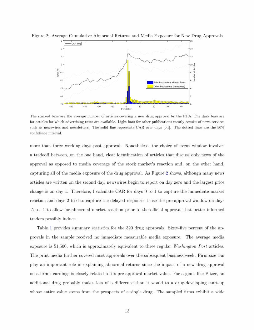
Figure 2: Average Cumulative Abnormal Returns and Media Exposure for New Drug Approvals
−40 −30 −20 −10 0 10 20 30 40−5
−4
−3
−2
−1
0
1
2
3
Event Day
CA
R (
%)
CAR [0,t]
0
2
4
6
8
10
12
14
16
Num
ber
of A
rtic
les
Print Publications with Ad Rates
Other Publications (Newswires)
The stacked bars are the average number of articles covering a new drug approval by the FDA. The dark bars are
for articles for which advertising rates are available. Light bars for other publications mostly consist of news services
such as newswires and newsletters. The solid line represents CAR over days [0,t]. The dotted lines are the 90%
confidence interval.
more than three working days past approval. Nonetheless, the choice of event window involves
a tradeoff between, on the one hand, clear identification of articles that discuss only news of the
approval as opposed to media coverage of the stock market’s reaction and, on the other hand,
capturing all of the media exposure of the drug approval. As Figure 2 shows, although many news
articles are written on the second day, newswires begin to report on day zero and the largest price
change is on day 1. Therefore, I calculate CAR for days 0 to 1 to capture the immediate market
reaction and days 2 to 6 to capture the delayed response. I use the pre-approval window on days
-5 to -1 to allow for abnormal market reaction prior to the official approval that better-informed
traders possibly induce.
Table 1 provides summary statistics for the 320 drug approvals. Sixty-five percent of the ap-
provals in the sample received no immediate measurable media exposure. The average media
exposure is $1,500, which is approximately equivalent to three regular Washington Post articles.
The print media further covered most approvals over the subsequent business week. Firm size can
play an important role in explaining abnormal returns since the impact of a new drug approval
on a firm’s earnings is closely related to its pre-approval market value. For a giant like Pfizer, an
additional drug probably makes less of a difference than it would to a drug-developing start-up
whose entire value stems from the prospects of a single drug. The sampled firms exhibit a wide
13

Table 1: New Drug Approvals Sample Summary Statistics
Mean Std Min 25th % Median 75th % Max N
Media Exposure 1.50 4.31 0 0 0 0.78 31.96 320Subsequent Media Exposure 2.17 3.39 0 0 1 2.63 20.92 320Preceding Media Exposure 0.14 0.58 0 0 0 0 5.18 320WSJ News Pressure 18.57 3.44 13.25 16.29 17.60 20.38 29.20 320Market Cap (Millions $) 28064 34622 18 1774 16401 39211 194823 320
The sample includes 320 Original New Drug Approvals over the years 1990-2007 marked by the FDA as New Molecular
Entity applications. Media Exposure is the sum of all articles on the approval day and the following day, weighted
by an adjacent advertising rate and presented in thousands of dollars. Subsequent Media Exposure is calculated
similarly for days 2 to 6, as is Preceding Media Exposure for days -5 to -1. WSJ News Pressure is the 40-day moving
average of the number of pages in section A of the Wall Street Journal one day after the approval. Market Cap is the
sponsoring firm’s market capitalization in millions of 1990 dollars one year before the event. If data are not available
for that time then the first day with data within that year is used instead.
Table 2: Returns and Volume around Approvals
Mean t-stat Std Min Median Max Per-day N
Pre-Approval CAR (R1) 1.33 3.75 6.34 -18.07 0.63 39.13 0.27 320Approval CAR (R2) 1.35 4.32 5.59 -18.61 0.60 47.08 0.68 320Post-Approval CAR (R3) -0.53 -1.62 5.86 -30.00 -0.14 22.72 -0.11 320
Historical Turnover 0.52 14.12 0.58 0.04 0.31 5.43 0.52 248Pre-Approval CATO (T1) 0.56 2.36 3.79 -3.79 -0.56 28.28 0.11 255Approval CATO (T2) 2.02 4.92 6.55 -1.41 -0.13 54.82 0.40 255Post-Approval CATO (T3) 1.29 3.53 5.84 -3.91 -0.48 52.27 0.26 255
CAR [a,b] is cumulative abnormal percent return over event trading days a to b, where abnormal return is return in
excess of the value-weighted market portfolio. CATO [a,b] is cumulative abnormal percent turnover, where abnormal
turnover is turnover in excess of market portfolio turnover. Turnover data is not available for ADRs. Pre-Approval
window is [-5,-1]. Approval window is [0,1]. Post-Approval window is [2,6]. Historical Turnover is the security’s past
year average daily percent turnover up to day -12. Per-day is the mean divided by the number of cumulation days.
variation in size measured as market capitalization one year before the approval in 1990 dollars,
with a $28 billion average.
Using the sample averages in Table 2, we can discern several interesting features of drug ap-
provals. The average drug approval generated a 1.33% abnormal return in the pre-approval period.
Upon approval, it returned an additional 1.35% and then declined 0.53% over the subsequent five
trading days. Since the standard errors of the pre-approval and approval means are small, we can
reject that they are zero at usual significance levels. About half of the price appreciation occurs
before the drug is officially approved which is indicative of superiorly informed agents participating
in the market. The post-approval abnormal return of the average drug is statistically no differ-
ent from zero. When we do not condition on any information other than the approval itself, the
14

Figure 3: Media Exposure Sub-Samples
−40 −30 −20 −10 0 10 20 30 40−5
−4
−3
−2
−1
0
1
2
3
4
5
Event Day
CA
R [0
,t] (
%)
No Media ExposureLow Media ExposureHigh Media Exposure
High media exposure sub-sample is the top half of drug approvals with positive media exposure on days 0 and 1
containing 56 observations. Low contains the bottom 57 observations with positive media exposure. No media
exposure contains the remaining 207 observations. The plotted average cumulative abnormal returns are normalized
to zero one day before the approval. Abnormal returns are in excess of those of the value-weighted market portfolio.
market’s reaction is consistent with semi-strong market efficiency.
However, if we condition on a certain level of media exposure, the picture is different. In Figure 3,
I split the sample into high, low, and zero media exposure sub-samples. Recall that media exposure
is measured on the approval day and the next. All three sub-samples feature a price increase in the
days before the approval. The pre-approval return seems higher for drugs that would later appear in
the news. This suggests insider-trading activity is increasing in future media exposure. At approval
time, drugs covered by the media exhibit a higher price increase than the rest. Post-approval, the
stock price of drug sponsors that received no initial media exposure continue to appreciate while
low-media-exposure firms maintain their valuation. Interestingly, high-media-exposure approvals
exhibit a negative drift following the approval, which continues even at a longer horizon than the
one I test below. These results suggest variation in media exposure is related to the path of price
adjustment to news.
4 Structural Estimation
In this section, I apply the simulated method of moments of Duffie and Singleton (1993) as described
in Gourieroux, Monfort, and Renault (1993) to the cross-section of drug approvals and their short
time series around approvals. I investigate whether the effects of the diffusion of information on
15

returns and volume the model implies are quantitatively important and in line with those in the
data. The goal of this exercise is to find a set of model parameters that generate moments close to
those in the data. By defining a clear loss function that can be used to judge the fit of the model to
the data, this exercise can guide future improvement of the theory (Hansen and Heckman, 1996).
4.1 Parameterization and Sample Selection
I begin by parameterizing the incidence probability as follows:
Γ(I; δ) = δIn, (6)
where δ ∈ [0, 1] is the transmission rate of the information specific to each drug approval. It
parametrizes public interest in the news. The elasticity of Γ(I) with respect to I is parametrized
by n ≥ 0. It has an intuitive interpretation as the number of informed agents required for effec-
tive information transmission to a randomly matched uninformed agent. One can think of more
complicated news as requiring more than a one-on-one meeting for transmission. The information
percolation literature studies the aggregation of information in a random matching environment
and shows that agents’ posterior beliefs evolve according to a similar process (Duffie and Manso,
2007).
The sample of drug approvals is selected because no denied approval requests are in my sample.
To account for this selection, I use only the right tail of the signal distribution. Specifically,
θj = µ0 + τ− 1
20 υj , (7)
where υj is a truncated Gaussian restricted to be positive. Thus all the news simulated is positive
news, just as in the sample.
4.2 Media Exposure as a Proxy for the Transmission Rate
I next parameterize the transmission rate of information which is known to agents but hidden to
the econometrician, and relate it to media coverage.
A news cycle at a modern newspaper like the Wall Street Journal begins when the production
16

department allocates a certain number of columns for the editors to fill with news in the next
day’s edition. This space in the book plan between the ads is called the newshole. The amount of
advertising sold and the availability of news determine its size. Newspapers have a target average
advertising-to-news ratio they aim for on a weekly, or quarterly basis. Within this pre-specified
newshole, the editors must decide what stories are newsworthy enough to be published. More
interesting news features more prominently, say, on the front page, whereas other news is relegated
to inner pages. At times of major news events such as election cycles or natural disasters, editors
request additional space for news. When they do so, they compensate by reducing the amount of
news on other days to maintain their target.6
Furthermore, since the editor cannot publish a marginal article, for example, just a word or two
about the story, some stories will not make it into the news at all. With this additional constraint,
media coverage is actually either positive if the story is interesting enough to pass the threshold,
or is exactly zero. The editor must pick the day’s most interesting stories and discard or postpone
publication of the rest. Thus each story’s chances of being published in a prominent section of the
newspaper depends critically on the availability of other competing stories.
Consequently, I model the media coverage of a drug approval story as an increasing function
of how interesting it is, which determines its transmission rate in the population, and a decreasing
function of the availability of other newsworthy material. Let mj denote the media coverage of
drug j:
mj = max
0,xTj βm + γzj + logit (δj), (8)
where δj ∼ Beta(αδ, βδ) is the transmission rate of the news story with positive shape and scale
parameters αδ and βδ. This distributional assumption for the transmission rate is necessary in
order to restrict it to the range (0, 1). With the fixed cost, the observable outcome is a media
coverage censored at zero. This censoring is apparent in Table 1. It can be the result of a fixed
cost in publishing a story or of measurement. The logit function provides a one-to-one mapping
from δ ∈ (0, 1) to the entire real line, as is common in probability models. This functional form
means media coverage is more sensitive to variation in transmission rates around the boundaries of
6Special thanks to Jim Pensiero and Robin Haynes of the Wall Street Journal for explaining this process.
17

Table 3: Censored Media Coverage Model ML Estimates
mj = max
0,xTj βm + γzj + logit (δj)
δ ∼ Beta(αδ, βδ)
γ αδ βδ N
-0.71** 0.30 0.25*** 320[0.36] [0.24] [0.02]
Reported are maximum likelihood estimates from the censored media coverage model. Controls in xj include a
constant, firm size, and year and month fixed-effects. zj is the WSJ News Pressure one day after the approval, which
proxies for the availability of other newsworthy material. Standard errors are in brackets.
its support. Specification (8) allows me to use media coverage as a proxy for the transmission rate.
The availability of other newsworthy material crowds out the exposure an approval gets. To
capture the editor’s outside option zj , I use WSJ News Pressure defined as the 40-day moving
average of the number of pages in section A of the Wall Street Journal published on day 1 when
drug-approval newspaper coverage usually appears.7 This exogenous variation allows me to identify
the parameters of the δ distribution by crowding out media exposure for some observations below
the censoring threshold. Maximum likelihood estimation is a straightforward exercise given this
model. I include in the control vector xj a constant, firm size, and year and month fixed-effects.
Table 3 reports MLE estimated parameters and their standard errors. As expected, WSJ News
Pressure is negatively correlated with media exposure. The point estimate γ = −0.71 (s.e. 0.36) is
negative and significant consistent with news pressure crowding out approval news.
Ideally, I would proceed by including conditional distributions of returns and volume given the
parameters of the model and maximize the likelihood that the process generating the sample of
drug approvals is the gradual information diffusion model. However, MLE requires distributional
assumptions about residuals on which I have no strong prior. I instead proceed by using the cross
section of latent transmission rates δ from MLE estimation of (8) as input to the indirect inference
procedure. Observations where media exposure is positive use the residual after controlling for
other sources of variation. Censored observations use the expected value of δ, which is a non-linear
7This measure of news pressure is related to the television news pressure instrument constructed in Eisensee andStromberg (2007) that proxies for the availability of newsworthy material also using a 40-day moving average of dailyTV news pressure defined as the median (across broadcasts in a day) number of minutes a news broadcast devotesto the top three news segments in a day. In addition, the authors use Olympic games incidence as a second sourceof variation. In unreported results, I find that TV news pressure does not crowd out drug approval news, perhapsbecause major TV networks cater to a different clientele than that of the business press I try to capture with myinstrument. Olympic games do crowd out drug-approval news, but only coincide with 8 drug approvals in my sample.Recent uses of this idea include Hirshleifer, Lim, and Teoh (2009) and Soltes (2009).
18

function of x and z. Specifically, the transmission rate of drug approval j is
δj =
logistic
(mj − xTj βm − γzj
)mj > 0
E [δ|xj , zj ,mj ≤ 0] mj = 0,
where E [δ|x, z,m ≤ 0] = Beta[logistic(−xTβm−γz),αδ+1,βδ]Beta[logistic(−xTβm−γz),αδ,βδ]
.
4.3 Indirect Inference
My identification strategy relies on observable variation in transmission rates as proxied by the
media exposure of various drug approvals. For different transmission rates the model predicts a
different price path as news of a drug approval are gradually incorporated into prices. The total
average price increase is the same regardless of δ, but the time signature of prices varies. Variation
in δ also affects the degree of heterogeneity in information sets, which results in different time
series of turnover. The parameters of the model determine how transmission rates affect observable
returns and turnover.
Moments I choose to match include mean cumulative abnormal returns as well as the mean
cumulative abnormal turnover of the first two periods. The model counterpart to abnormal return
is the realized return less the expected risk premium Ret ≡ Qt −E0 [Qt] . In addition, I include the
mean product of returns with δ, to capture the dependence of these outcomes on the transmission
rate of information. Since by assumption agents know δ, the difference between the observed returns
and those predicted by the model is orthogonal to δ. Turnover moments are especially informative
about the supply shocks variance. The levels of abnormal returns change considerably when the
precision of the signal τ0 changes. Covariance of returns with transmission rates is informative
about the fraction that is early informed and by the competitive information market assumption
about the cost of information acquisition. Finally, I include second moments that capture the
autocorrelation of returns.
To gain some intuition for the sources of parameter identification, Figure 4 contrasts slow-
diffusing (δ = 0) positive news with fast-diffusing ones (δ = 1). The source of the main difference
between the two is the informed fraction at time 2. This is the direct effect of δ. The cost of
information c determines the fraction informed at time 1 which is sensitive to δ, though these
19
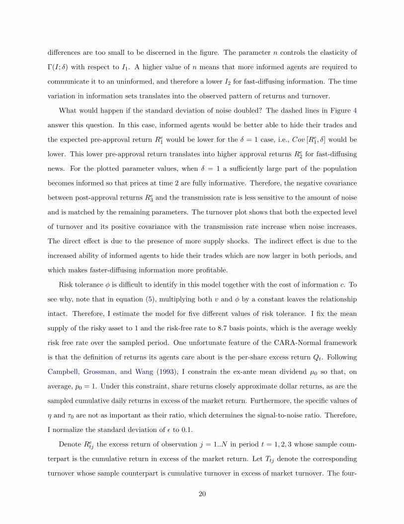
differences are too small to be discerned in the figure. The parameter n controls the elasticity of
Γ(I; δ) with respect to I1. A higher value of n means that more informed agents are required to
communicate it to an uninformed, and therefore a lower I2 for fast-diffusing information. The time
variation in information sets translates into the observed pattern of returns and turnover.
What would happen if the standard deviation of noise doubled? The dashed lines in Figure 4
answer this question. In this case, informed agents would be better able to hide their trades and
the expected pre-approval return Re1 would be lower for the δ = 1 case, i.e., Cov [Re1, δ] would be
lower. This lower pre-approval return translates into higher approval returns Re2 for fast-diffusing
news. For the plotted parameter values, when δ = 1 a sufficiently large part of the population
becomes informed so that prices at time 2 are fully informative. Therefore, the negative covariance
between post-approval returns Re3 and the transmission rate is less sensitive to the amount of noise
and is matched by the remaining parameters. The turnover plot shows that both the expected level
of turnover and its positive covariance with the transmission rate increase when noise increases.
The direct effect is due to the presence of more supply shocks. The indirect effect is due to the
increased ability of informed agents to hide their trades which are now larger in both periods, and
which makes faster-diffusing information more profitable.
Risk tolerance φ is difficult to identify in this model together with the cost of information c. To
see why, note that in equation (5), multiplying both v and φ by a constant leaves the relationship
intact. Therefore, I estimate the model for five different values of risk tolerance. I fix the mean
supply of the risky asset to 1 and the risk-free rate to 8.7 basis points, which is the average weekly
risk free rate over the sampled period. One unfortunate feature of the CARA-Normal framework
is that the definition of returns its agents care about is the per-share excess return Qt. Following
Campbell, Grossman, and Wang (1993), I constrain the ex-ante mean dividend µ0 so that, on
average, p0 = 1. Under this constraint, share returns closely approximate dollar returns, as are the
sampled cumulative daily returns in excess of the market return. Furthermore, the specific values of
η and τ0 are not as important as their ratio, which determines the signal-to-noise ratio. Therefore,
I normalize the standard deviation of ε to 0.1.
Denote Retj the excess return of observation j = 1..N in period t = 1, 2, 3 whose sample coun-
terpart is the cumulative return in excess of the market return. Let Ttj denote the corresponding
turnover whose sample counterpart is cumulative turnover in excess of market turnover. The four-
20
Figure 4: Slow vs. Fast Diffusing News
æ æ æ
æ
à à
à à
æ æ æ
æ
à à
à à
0 1 2 3t
0.2
0.4
0.6
0.8
1.0
I t
Informed Fraction
æ æ æ
æ
à
àà
à
æ æ æ
æ
à
à
à
à
0 1 2 3t
1.02
1.04
1.06
1.08
E@ P t ÈD0 >0D Price
æ æ æ
æ
à
à
ààæ æ æ
æ
à
à
à
à
1 2 3t
0.5
1.0
1.5
2.0
2.5
3.0
E@ R te ÈD0 >0D Excess Share Returns
æ
æ
æ
æ
à
à
à
à
æ
æ
æ
æ
à
à
à
à
0 1 2 3t
0.5
1.0
1.5
2.0
2.5
3.0
E@T t ÈD0 >0D Turnover
à ∆ =1.0
æ ∆ =0.0
The plots contrast slow-diffusing (δ = 0) positive news with fast-diffusing ones (δ = 1). Excess share returns and
turnover are presented in percent. The solid lines use the parameters estimated in Section 4. The dashed lines use
the same parameters but double the standard deviation of noise.
21

period gradual information diffusion model in Section 2, for each observation j, maps the exogenous
observable δj , unobservable shocks uj = [θj , x1j , x2j , εj ], and model parameters α = [ξ, τ0, v, n] into
a vector of endogenous observables yj = [Re1j , Re2j , Re3j , T1j , T2j , T3j ] = r(δj , uj , α). The shocks are
just a linear function uj = ϕ(υj , α) of a vector of i.i.d Gaussian noise υj .
Let kj = k(yj , δj) denote the multidimensional function of the data with associated empirical
moments kN = 1N
∑Nj=1 k(yj , δj). Specifically, my choice of moments is
kN = 1N
N∑j=1
[Re1j , Re2j , Re3j , T1j , T2j , Re1jδj , Re2jδj , Re3jδj , Re1jR
e2j , Re2jR
e3j
]T.
Simulated moments are similarly calculated conditional on the same sample δs, but with yhj (α) =
r(δj , u
hj (α), α
), where h = 1 . . . H indexes simulations. That is, yhj depends on the random draw
of υhj and on the parameters α. Thus the numerical optimization procedure attempts to match
10 moments with 4 free parameters. The additional moments provide overidentifying restrictions.
The indirect estimator αHN is obtained by minimizing
minα
kN − 1NH
N∑j=1
H∑h=1
k(yhj (α), δj
)T kN − 1NH
N∑j=1
H∑h=1
k(yhj (α), δj
) .For each δj , I simulate H = 10000 different random draws of shocks. Since I have no reason to
favor one moment over another, I use the identity matrix as a weighting matrix.
4.4 Estimation Results
Table 4 presents indirect estimation results for five different values of risk tolerance. The mean
payoff µ0 is constrained by the other parameters so the ex-ante price p0 = 1. More risk-averse agents
require a higher expected payoff to value the risky asset at the same price. Both the precision of
the supply shocks ξ and that of the signal τ0 are decreasing in risk aversion. By examining the
values of the minimized objective, we can see the model with risk aversion φ−1 = 5 performs better
than the rest, and I therefore focus on these results for the remainder of the analysis.
With a constant absolute risk aversion of 5, the cost of inside information is about 53% of
an uninformed agent’s position in the risky asset at time 1. This cost can be interpreted as the
expected cost of trading on private information with a chance of adverse legal consequences. On
22

Table 4: Indirect Estimation Results
φ−1 E[θ] σ[xt] σ[θ] c n Objective
0.5 1.008 0.010 0.029 1.439 0.367 5.850[0.000] [0.002] [0.148] [0.018]
1.0 1.013 0.013 0.018 1.389 0.104 6.189[0.001] [0.001] [0.078] [0.009]
2.5 1.029 0.016 0.026 1.055 0.008 5.512[0.001] [0.006] [0.053] [0.004]
5.0 1.060 0.013 0.038 0.528 0.000 4.792[0.001] [0.003] [0.045] [0.014]
10.0 1.117 0.012 0.038 0.202 0.001 4.841[0.001] [0.007] [0.012] [0.015]
Reported are indirect inference parameter estimates each using five different values of absolute risk tolerance φ. Each
optimization uses the 255 observations times 10000 simulated shock draws. The mean payoff E[θ] = µ0 is constrained
given the other parameters so that p0 = 1. The standard deviation of the the unobservable component is normalized
to σ [ε] = 0.1. σ [xt] is the standard deviation of the supply shocks. σ [θ] is the standard deviation of the signal θ at
time 0. c is the fixed cost of information. n is the elasticity of the incidence probability Γ(I1; δ) w.r.t to the fraction
informed at time 1. Objective is the value of the minimized quadratic objective. Standard errors are in brackets.
average, agents informed about a drug approval before the official announcement control only a tiny
fraction of invested wealth; it is on the order of 10−6. The signal-to-noise ratio for the average drug
approval V ar[θ]V ar[θ]+V ar[ε] is 12%, which means the reduction in uncertainty about the value of the drug
developing firm that is associated with an approval is small relative to the remaining uncertainty.
This ratio is consistent with DiMasi (2001), which studies the drug approval process and estimates
the probability that a drug will be approved conditional on surviving to phase III trials is about
75%.
Non-informational supply shocks have a standard deviation of 1% of the total supply of the stock.
Compared with the 6.5% standard deviation of approval turnover in the sample, this number is
small. Thus the model requires only a small amount of non-informational trading to prevent prices
from fully revealing the news.8
Table 5 provides a comparison between sample moments and their simulated counterparts using
the estimated parameters. The goal of the numerical procedure is to minimize the discrepancy
between the two, which I report in the last column. The covariances are those implied by the 10
matched moments and the average δ of 0.54.
8Since there are no borrowing constraints in the model, informed agents can hold a highly levered position attime 1 to exploit their informational advantage. The more these agents can borrow, the more informative are prices.Extending the model to incorporate borrowing constraints will decrease the required amount of noise. Therefore, ina sense, this estimate of the standard deviation of the supply shocks is an upper bound.
23
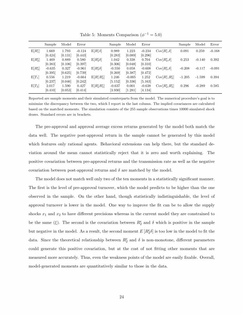
Table 5: Moments Comparison (φ−1 = 5.0)
Sample Model Error Sample Model Error Sample Model Error
E[Re1] 1.669 1.793 -0.124 E[Re1δ] 0.989 1.223 -0.234 Cov[Re1,δ] 0.091 0.259 -0.168[0.424] [0.131] [0.443] [0.283] [0.089] [0.296]
E[Re2] 1.469 0.889 0.580 E[Re2δ] 1.042 0.338 0.704 Cov[Re2,δ] 0.253 -0.140 0.392[0.383] [0.106] [0.397] [0.306] [0.048] [0.310]
E[Re3] -0.635 0.327 -0.961 E[Re3δ] -0.550 0.058 -0.608 Cov[Re3,δ] -0.208 -0.117 -0.091[0.395] [0.625] [0.739] [0.269] [0.387] [0.472]
E[T1] 0.556 1.219 -0.664 E[Re1Re2] 1.246 -0.005 1.252 Cov[Re1,Re2] -1.205 -1.599 0.394
[0.237] [0.046] [0.242] [5.152] [0.336] [5.163]E[T2] 2.017 1.590 0.427 E[Re2R
e3] -0.637 0.001 -0.638 Cov[Re2,Re3] 0.296 -0.289 0.585
[0.410] [0.053] [0.414] [3.930] [1.281] [4.134]
Reported are sample moments and their simulated counterparts from the model. The numerical procedure’s goal is to
minimize the discrepancy between the two, which I report in the last column. The implied covariances are calculated
based on the matched moments. The simulation consists of the 255 sample observations times 10000 simulated shock
draws. Standard errors are in brackets.
The pre-approval and approval average excess returns generated by the model both match the
data well. The negative post-approval return in the sample cannot be generated by this model
which features only rational agents. Behavioral extensions can help there, but the standard de-
viation around the mean cannot statistically reject that it is zero and worth explaining. The
positive covariation between pre-approval returns and the transmission rate as well as the negative
covariation between post-approval returns and δ are matched by the model.
The model does not match well only two of the ten moments in a statistically significant manner.
The first is the level of pre-approval turnover, which the model predicts to be higher than the one
observed in the sample. On the other hand, though statistically indistinguishable, the level of
approval turnover is lower in the model. One way to improve the fit can be to allow the supply
shocks x1 and x2 to have different precisions whereas in the current model they are constrained to
be the same (ξ). The second is the covariation between Re2 and δ which is positive in the sample
but negative in the model. As a result, the second moment E [Re2δ] is too low in the model to fit the
data. Since the theoretical relationship between Re2 and δ is non-monotone, different parameters
could generate this positive covariation, but at the cost of not fitting other moments that are
measured more accurately. Thus, even the weakness points of the model are easily fixable. Overall,
model-generated moments are quantitatively similar to those in the data.
24

Figure 5: The Value of Information Diffusing at Rate δ
0.0 0.2 0.4 0.6 0.8 1.0∆
0.1
0.2
0.3
0.4
0.5
0.6
v H∆L
v3
v2
v1
0.000 0.002 0.004 0.006 0.008 0.010∆
0.01
0.02
0.03
0.04
v H∆L
v3
v2
v1
The plot on the left decomposes the value of information according to (5) as a function of the transmission rate
based on the average informed fraction in the simulated sample (I1 = 2.44 × 10⁻⁶). The plot on the right focuses
on the limit as δ vanishes. The first, and empirically dominant term, is due to the intertemporal growth rate of
uninformed agents’ precision about returns. The second term is due to the intertemporal increase in precision of the
informed relative to this increase by the uninformed. The third term represents the extent of information spillover
to uninformed agents who do not pay for the signal. Parameters are those estimated in Section 4.
4.5 The Implied Market for Information
Proposition 3 decomposes the value of information into three terms. We can use the parameter
estimates to get a sense of their relative magnitude. Figure 5 presents a decomposition based on the
average informed fraction in the simulated sample. For an average transmission rate, the first term is
0.62, whereas the second and third terms are on the order of 10−5. Thus at least in the neighborhood
of the estimated parameters, the value of information stems entirely from the intertemporal growth
rate of uninformed agents’ precision Ωv. This growth is not exogenous but rather an equilibrium
outcome. Because it is the dominant term of the value of information, given the constant cost of
information c, either there are no informed in equilibrium, or Ωv = τ2+ητ1≈ e
2φR2c
, which implies
the ratio τ2τ1
is kept constant across the various transmission rates.
The right panel allows us to examine the limiting behavior of the value of information as δ → 0,
i.e. when information does not diffuse. This limiting value of information is about fifty times
smaller than at the average transmission rate. Therefore the transmission rate of information has
a quantitatively important effect on the value of information.
This nature of investor demand for information together with the fixed cost of acquiring it
produce an interesting equilibrium outcome in the market for information plotted in Figure 6. The
plots show that no information is acquired in equilibrium when δ is low, that is, for uninteresting
25

Figure 6: The Market for Information
0.0000 0.0002 0.0004 0.0006 0.0008 0.0010I1
0.5
0.6
0.7
0.8
ΝH I1 ; ∆L
∆ =0.2
∆ =0.4
∆ =0.8
Supply
0.2 0.4 0.6 0.8 1.0∆
0.0001
0.0002
0.0003
0.0004
0.0005
0.0006
I1*
The plot on the left shows demand for information v(I1; δ) as a function of the percent of population informed I1
for three different values of δ. The dashed line indicates the constant supply price. The plot on the right shows the
equilibrium informed percent of population. Parameters are those estimated in Section 4.
news. Around δ = 0.25, the fraction informed rises sharply and then slowly declines. Thus faster-
diffusing information is purchased at a high rate, while the fastest-diffusing news is less valuable.
The elasticity n is estimated at 0.0001 and is statistically no different from zero (Table 4),
but an exact zero cannot generate the negative covariation between post-approval returns and
the transmission rate. The parametrization of the incidence probability in (6) has a discontinuity
at n = 0. When n is zero, a meeting with an informed agent is not necessary for information
transmission. A high δ results in a high I2 even if I1 is close to zero. However, when n approaches
zero from the right, a small I1 implies a small I2 regardless of δ. Unreported attempts to generate
the covariance pattern in the data with n = 0 have been unsuccessful. The data is telling us that
a simpler discontinuous model of the incidence probability along the lines of Γ(I1; δ) = δ × 1I1>0
might suffice.
Matching the magnitudes of covariation between the transmission rate proxied by media expo-
sure and stock returns additionally requires information choice. The fixed cost affects the extensive
margin and creates two effective types of news, one with positive equilibrium information acquisi-
tion in which pre-approval returns are high and post-approval returns are low, and another type
with no private information. Thus endogenous information acquisition accentuates the covariation
between the transmission rate of information and returns.
26
4.6 Discussion of Limitations and Directions for Future Research
As usual, structural estimates are hard to interpret outside their model. If, for example, one
moved beyond the CARA-Normal framework, the model’s predictions might change. Relaxing the
CARA utility assumption could introduce wealth effects (Peress, 2004). Under non-Normal payoff
distributions, the theoretical results might change since price-informativeness could decrease with
the fraction informed (Barlevy and Veronesi, 2000). Normality also imposes structure on empirical
error terms, though relaxing this assumption should not have a big effect on large sample estimates.
I abstract from several other realistic features of the world to gain an estimable model that
captures the main forces at play during drug approvals. For example, the cost of information c
could potentially be different across events. The informed fraction would be smaller for more costly
pieces of information. I have tried to control for important potential sources of heterogeneity by
including controls for firm size, news pressure, and time effects. However, if information costs
and transmission rates are correlated in a way not captured by these controls, then the estimates
could be biased. This is less of a concern here, since the largest cost of information likely stems
from an expected utility loss from incarceration, which applies similarly to all drug approvals.9
But, this potential heterogeneity could be important for other events. Other sources of unobserved
heterogeneity such as signal-to-noise ratios can either be modeled as random effects, like I treat
cash flow news heterogeneity above, or treated directly with instruments.
Another limitation is endogeneity. The estimation exploits variation in transmission rates of
information as proxied by media coverage, assuming that transmission rates are exogenous and
determine media coverage. One reasonable alternative approach would be to allow media coverage
to further depend on the expectations of journalists about future price swings. Introducing such a
dependency in (8) could potentially alter my estimates. Similarly, the interpersonal transmission
rate of information might increase or decrease with the profitability of informed trading. To some
extent this is already in the model since the incidence probability depends on the informed fraction
which responds to such profitability. To cleanly identify the direction of causality without such
structure, one could use exogenous sources of variation in transmission rates, but doing this correctly
is easier said than done. Ultimately, we strive for a model that is both theoretically sound and fits
9An FDA chemist was recently sentenced to five years in prison for insider-trading on drug-approval information(Schoenberg, 2012).
27

the data well. This paper is merely a step in this direction. Structural estimation of alternative
models can be a promising avenue for further study.
5 Conclusion
Based on the above analysis let us revisit the question, how much to pay to know today that
Viagra as opposed to Allegra will be approved tomorrow. The answer turns out to depend on
how fast exactly news of each approval diffuses, through its effect on the intertemporal decline in
uncertainty. The transmission rate has two contrasting effects. The first and more intuitive effect
is that unlike for obscure drugs, private information about Viagra’s approval will surely be quickly
reflected in prices allowing for a quick and safe profit. However, a second effect of this potential gain
is that informed agents trade more aggressively, which makes pre-approval prices more informative.
This decline in uncertainty for fast diffusing news reduces the equilibrium value of information.
Empirically, the estimated value of information turns out to be hump-shaped in the transmission
rate of information.
References
Admati, Anat R, and Paul Pfleiderer, 1986, A monopolistic market for information, Journal ofEconomic Theory 39, 400 – 438.
Admati, Anat R., and Paul Pfleiderer, 1988, Selling and trading on information in financial markets,The American Economic Review 78, pp. 96–103.
Barlevy, Gadi, and Pietro Veronesi, 2000, Information acquisition in financial markets, The Reviewof Economic Studies 67, 79–90.
Birkhoff, Garrett, and Saunders Mac Lane, 1997, A Survey of Modern Algebra (A. K. Peters) 5thedn.
Campbell, John Y., Sanford J. Grossman, and Jiang Wang, 1993, Trading volume and serial cor-relation in stock returns, The Quarterly Journal of Economics 108, 905–939.
Cho, Jin-Wan, and Murugappa Krishnan, 2000, Prices as aggregators of private information: Evi-dence from s&p 500 futures data, Journal of Financial and Quantitative Analysis 35, 111–126.
Cohen, L., A. Frazzini, and C. Malloy, 2008, The small world of investing: Board connections andmutual fund returns, Journal of Political Economy 116, 951–979.
Colla, Paolo, and Antonio Mele, 2010, Information linkages and correlated trading, Review ofFinancial Studies 23, 203–246.
28

Daley, Brendan, and Brett Green, 2012, Waiting for news in the market for lemons, Econometrica80, 1433–1504.
DellaVigna, Stefano, and Joshua M. Pollet, 2009, Investor Inattention and Friday Earnings An-nouncements, Journal of Finance 64, 709–749.
DiMasi, Joseph A., 2001, Risks in new drug development: approval success rates for investigationaldrugs, Clinical Pharmacology and Therapeutics 69, 297–307.
Dow, James, Itay Goldstein, and Alexander Guembel, 2011, Incentives for information productionin markets where prices affect real investment, Working Paper.
Duffie, Darrell, Semyon Malamud, and Gustavo Manso, 2009, Information percolation with equi-librium search dynamics, Econometrica 77, 1513–1574.
, 2010, The relative contributions of private information sharing and public information re-leases to information aggregation, Journal of Economic Theory 145, 1574 – 1601 <ce:title>SearchTheory and Applications</ce:title>.
Duffie, Darrell, and Gustavo Manso, 2007, Information percolation in large markets, AmericanEconomic Review P&P 97, 203–209.
Duffie, Darrell, and Kenneth J. Singleton, 1993, Simulated moments estimation of markov modelsof asset prices, Econometrica 61, 929–952.
Easley, David, and Maureen O’hara, 2004, Information and the cost of capital, The Journal ofFinance 59, 1553–1583.
Eisensee, Thomas, and David Stromberg, 2007, News Floods, News Droughts, and US DisasterRelief, Quarterly Journal of Economics 122, 693–728.
Fishman, M.J., and K.M. Hagerty, 1995, The incentive to sell financial market information, Journalof Financial Intermediation 4, 95 – 115.
Garcia, Diego, and Joel M. Vanden, 2009, Information acquisition and mutual funds, Journal ofEconomic Theory 144, 1965 – 1995.
Garcıa, Diego, and Francesco Sangiorgi, 2011, Information sales and strategic trading, Review ofFinancial Studies 24, 3069–3104.
Garcıa, Diego, and Gunter Strobl, 2011, Relative wealth concerns and complementarities in infor-mation acquisition, Review of Financial Studies 24, 169–207.
Gourieroux, C., A. Monfort, and E. Renault, 1993, Indirect inference, Journal of Applied Econo-metrics 8, S85–S118.
Gray, Wesley R., 2010, Do Hedge Fund Managers Identify and Share Profitable Ideas?, WorkingPaper.
Grossman, Sanford J., 1995, Dynamic asset allocation and the informational efficiency of markets,The Journal of Finance 50, 773–787.
, and Joseph E. Stiglitz, 1980, On the impossibility of informationally efficient markets, TheAmerican Economic Review 70, 393–408.
29

Han, Bing, and Liyan Yang, forthcoming, Social networks, information acquisition, and asset prices,Management Science.
Hansen, Lars Peter, and James J. Heckman, 1996, The empirical foundations of calibration, TheJournal of Economic Perspectives 10, 87–104.
He, Zhiguo, and Asaf Manela, 2012, Information acquisition in rumor-based bank runs, WorkingPaper.
Hellwig, M.F., 1980, On the aggregation of information in competitive markets, Journal of economictheory 22, 477–498.
Hirshleifer, David, Sonya Seongyeon Lim, and Siew Hong Teoh, 2009, Driven to distraction: Ex-traneous events and underreaction to earnings news, The Journal of Finance 64, 2289–2325.
Hirshleifer, David, Avanidhar Subrahmanyam, and Sheridan Titman, 1994, Security analysis andtrading patterns when some investors receive information before others, The Journal of Finance49, 1665–1698.
Holden, Craig W., and Avanidhar Subrahmanyam, 2002, News events, information acquisition, andserial correlation, The Journal of Business 75, 1–32.
Hong, Dong, Harrison G. Hong, and Andrei Ungureanu, 2011, An Epidemiological Approach toOpinion and Price-Volume Dynamics, SSRN eLibrary.
Hong, Harrison, Jeffrey D. Kubik, and Jeremy C. Stein, 2005, Thy neighbor’s portfolio: Word-of-mouth effects in the holdings and trades of money managers, The Journal of Finance 60,2801–2824.
Hong, Harrison, and Jeremy C. Stein, 1999, A unified theory of underreaction, momentum trading,and overreaction in asset markets, The Journal of Finance 54, 2143–2184.
Kacperczyk, Marcin T., Stijn Van Nieuwerburgh, and Laura Veldkamp, 2012, Rational attentionallocation over the business cycle, Working Paper.
Kelly, Bryan, and Alexander Ljungqvist, 2012, Testing asymmetric-information asset pricing mod-els, Review of Financial Studies 25, 1366–1413.
Kyle, Albert S., 1985, Continuous auctions and insider trading, Econometrica 53, pp. 1315–1335.
Manela, Asaf, 2011, Spreading information and media coverage: Theory and evidence from drugapprovals, Ph.D. thesis University of Chicago.
Mele, Antonio, and Francesco Sangiorgi, 2011, Uncertainty, information acquisition and price swingsin asset markets, Working Paper.
Nieuwerburgh, Stijn Van, and Laura Veldkamp, 2009, Information immobility and the home biaspuzzle, The Journal of Finance 64, 1187–1215.
Ozsoylev, Han N., and Johan Walden, 2011, Asset pricing in large information networks, Journalof Economic Theory 146, 2252 – 2280.
Peress, Joel, 2004, Wealth, information acquisition, and portfolio choice, Review of Financial Stud-ies 17, 879–914.
30

Savov, Alexi, 2012, The price of skill: Performance evaluation by households, Working Paper.
Schoenberg, Tom, 2012, Fda chemist gets five years in prison for insider trading, .
Shiller, Robert J., and John Pound, 1989, Survey evidence on diffusion of interest and informationamong investors, Journal of Economic Behavior and Organization 12, 47–66.
Soltes, Eugene F., 2009, News dissemination and the impact of the business press, Ph.D. diss., TheUniversity of Chicago Graduate School of Business.
Stein, Jeremy C., 2009, Conversations among competitors, American Economic Review (forthcom-ing).
Tetlock, Paul C., 2007, Giving Content to Investor Sentiment: The Role of Media in the StockMarket, The Journal of Finance 62, 1139–1168.
U.S. Food and Drug Administration, 1998, CDER Manual of Policies and Procedures. Communi-cating Drug Approval Information, Online.
Van Nieuwerburgh, Stijn, and Laura Veldkamp, 2010, Information acquisition and under-diversification, The Review of Economic Studies 77, 779–805.
Veldkamp, Laura, 2006, Media frenzies in markets for financial information, The American Eco-nomic Review 96, 577–601.
, 2011, Information Choice in Macroeconomics and Finance (Princeton University Press).
Wang, Jiang, 1994, A model of competitive stock trading volume, The Journal of Political Economy102, 127–168.
A Model Solution and Omitted Proofs
A.1 Proof of Lemma 1 (Learning from Prices)
The inference problem of the uninformed is to form a posterior belief about the fundamental
value θ conditional on the current-period price. The prior belief of uninformed at time t is that
θ|pt ∼ N (µt, τ−1t ). The distribution of pt+1 conditional on θ can be attained by rearranging the
price conjecture: xt+1 = pt+1−at+1−bt+1∆t+1ct+1
∼ N (0, ξ−1). Substituting these into Bayes’ rule for the
posterior distribution of θ and solving for µt+1, which appears also in ∆t+1, yields the solution in
(4).
31

A.2 Proof of Proposition 1 (Existence of Equilibrium)
The proof of Proposition 1 proceeds in several steps. First, I conjecture that (3) holds and derive
agents’ beliefs given this conjecture. I then solve for agents’ optimal demand functions given their
beliefs starting with the final period and proceeding by backward induction. In each period, I
impose market clearing and verify the price functions satisfy the linear prices conjecture. Further
details can be found in Manela (2011).
After the payoff is revealed, should trading open for a claim to the payoff, the price must be
p3 = u. At that time, agents are again identical in the absence of wealth effects and I assume for
volume calculation purposes that qi3 = x for all i.
Period 2 of this model is identical to Grossman and Stiglitz (1980). Optimal holdings of the
risky asset are qi2 = φΨi2[Q3]Ei2[Q3], where the optimal asset holdings of type UI are the same
as those of type II even though the changes in their holdings, their demand, in period 2 can be
different. This time-varying heterogeneity is important for volume, but does not matter for prices
in the absence of wealth effects. Agents trade off the expected excess return per share with the
variance of the payoff that is scaled by φ, their risk tolerance. Substituting optimal demands into
the market-clearing condition at time 2 yields a linear price function p2 = p2(∆2, x2; p1). Matching
coefficients yields the three p2 coefficients:
a2 = µ1R− x
φR(I2ΨI
2[Q3] + U2ΨU2 [Q3]
) = µ1R− E0[Q3]
R
b2 = c2β2 = I2ΨI2[Q3]
R(I2ΨI
2[Q3] + U2ΨU2 [Q3]
) + ξβ22
Rτ1(9)
c2 = − 1φ(R− k2)
(I2ΨI
2[Q3] + U2ΨU2 [Q3]
) = − 1φR
(I2ΨI
2[Q3] + U2ΨU2 [Q3]
) + ξβ2Rτ1
Importantly, the ratio of the news coefficient b2 to the supply shocks coefficient c2 has a simple
expression β2 ≡ b2c2
= −φI2ΨI2[Q3] = −φI2η. The larger the magnitude of β2 in absolute value, the
more informative the price about the private information of the informed. This result shows that
p2 is more informative when agents are more tolerant of risk, which comes from holding the asset
well into the future. The level of risk depends on the residual uncertainty about the payoff. In
a multiple-asset model, this risk would come from the residual uncertainty about the systematic
component of the portfolio. Importantly, when I2 is high and more agents are informed at time 2
32
prices are more informative.
The choice of risky asset holdings at time 1 is somewhat more interesting yet harder to solve. In-
formed agents know they will remain informed in the future and therefore maximize V I1
(W I
1 ; ∆1, x1)
=
maxqI1
EI1
[V I
2
(W I
2 ; ∆2, x2)]. The problem of uninformed agents at time 1 involves additional uncer-
tainty about their informational type in period 2. Although the informed know they will remain
informed next period, the uninformed at time 1 may get the signal for free at the beginning of time
2. The uninformed agent’s problem at time 1 can be summarized by his value function:
V U1
(WU
1 ;µ1)
= maxqU1
EU1
[Γ (I1; δ)V I
2
(WU
2 ; ∆2, x2)
+ [1− Γ (I1; δ)]V U2
(WU
2 ;µ2)]. (10)
With probability Γ(I1; δ), the uninformed agent will receive the signal by period 2 and will then
use it to make his informed portfolio decision. The gain he expects from this future informational
advantage over less fortunate investors depends on the fraction informed both directly and indirectly.
The direct effect is simply due to the increase in the probability of observing the signal. The indirect
effect is from the reduction in uncertainty the signal provides by making prices more informative.
The exponential utility assumption allows us to express the expected informational advantage
of the informed over the uninformed in period 2 as follows:
EU2
[V I
2
]=
√τ2
η + τ2V U
2 . (11)
Due to the choice of a negative utility function, a larger proportionality term means a smaller
informational advantage. Intuitively, when the informed have more trading periods to use their
informational advantage, then its expected gain in utility is larger. The proportionality result in
(11), together with the law of iterated expectations, allow us to rewrite the uninformed agent’s
problem in (10) as follows:
V U1
(WU
1 ;µ1)
= maxqU1
[Γ (I1; δ)
√τ2τ2+η
+ (1− Γ (I1; δ))]EU1
[V U
2
(WU
2 ;µ2)].
Although this formulation greatly simplifies the problem, this special feature of the CARA-normal
framework also eliminates Γ(I1; δ) from the agent’s first-order condition for qU1 . Therefore, the
change in I only enters the uninformed portfolio problem indirectly, through its equilibrium effects
33

on means and variances.
An important feature of demand depends on the relationship between the period 2 excess return
and the period 2 expected excess return in period 3. This relationship takes the following linear
form:
Ei2[Q3] = Ei1[Q3] + ρi1
(Q2 − Ei1[Q2]
),
where the coefficients ρi1 for both types of agents are negative. Therefore Q2 is perfectly negatively
correlated with Ei2[Q3]. The intuition is easy to see for the informed agent whose expected payoff
at the final period does not change over time. From his perspective, any unexpected return in time
2 is due to the transitory supply shocks and he therefore expects it to reverse in the future. The
same force operates on the uninformed agent’s expectation, but his learning from prices attenuates
this effect. The reason is that the uninformed agent cannot fully distinguish between the transitory
supply shocks and the permanent news shocks that affect prices. Nonetheless, ρU1 is negative as
well since
k2 = R
ξφ2I2η(I2ΨI
2[Q3] + U2ΨU2 [Q3]
)τ1 + ξφ2I2η
(I2ΨI
2[Q3] + U2ΨU2 [Q3]
) < R,
and ρU1 = k2 −R < 0.
Faced with this opportunity set and full knowledge of the evolution of I over time, agents in
period 1 choose their optimal holdings of the risky asset. Optimal holdings of the risky asset by an
agent of type i going into period 2 are
qi1 = φ
R
(Ωi
1Ψi1[Q2]Ei1[Q2]− ρi1Ψi
2[Q3]Ei1[Q3]),
where Ωi1 ≡ 1 + Ψi2[Q3](ρi1)2
Ψi1[Q2] . The first term in parentheses can be interpreted as a myopic demand
component. Since Ωi1 is larger than one, agents demand more of the asset than if no further
uncertainty remained in period 2. Specifically, demand increases with the growth in precision,
or equivalently, when agents expect a sharper decrease in uncertainty from period 1 to period 2.
Agents also consider their continuation utility, which gives rise to the hedging demand component.
34

Since ρi1 is negative, a higher expected return in period 3 induces a higher demand for the asset in
period 1. Holding the asset to maturity provides a natural hedge since unexpectedly low returns
today are expected to be offset in the future.
Before examining the informativeness of prices, focusing on the expected return of an informed
agent in excess of the risk premium demanded by the uninformed (their alpha) is useful. In
the CARA-Normal framework, this conditional expected return can be expressed as a constant
multiplying the news:
EI1 [Q2]− EU1 [Q2] = G12∆1,
where the sensitivity of their informational expected return to news is G12 = b2τ1τ2
. The greater it
is, the greater the return following positive fundamental value shocks and conversely for negative
news.
The ratio of the news coefficient b1 to the supply shocks coefficient c1, which takes a more
elaborate form than before, determines the informativeness of p1. Specifically,
β1 ≡b1c1
= −φI1
(ΨI
2[Q3] + 1R
ΨI1[Q2]G12
). (12)
The first term in parenthesis is just as before but with the current fraction informed I1. As in β2,
the greater the risk tolerance or the greater the fraction informed at time 1, the more informative
p1 is about θ. Uncertainty about the payoff at time 3 again diminishes the informativeness of the
price. Additionally, the second component, which depends on the intermediate period 2, increases
the informativeness of p1. Prices are more informative when the opportunity cost of trading on
information, R, is small or when the informed are more certain about the intermediate return
Q2. Finally, the more sensitive the informed expected return EI1 [Q2] is to the news, the more
informative the price p1.
Since β1 = −φI1(k2R τ2 + η
), ∂β1∂I1
< 0, which confirms the intuition that the more informed
agents there are in period 1, the more informative prices are about this hidden signal. Further-
more, both ∂k2∂I2
> 0 and ∂τ2∂I2
> 0, which implies ∂β1∂I2
< 0 as well. That is, ceteris paribus, the
informativeness of prices at time 1 is increasing not only with the fraction informed at time 1, but
35

also with the fraction informed at time 2. The Kalman gain is
k1 = ξb1τ0c2
1= R2
ξφ2I1(k2τ2R + η
) (I1ΩI
1ΨI1[Q2] + U1ΩU
1 ΨU1 [Q2]
)R2τ0 + ξφ2I1
(k2τ2R + η
) (I1ΩI
1ΨI1[Q2] + U1ΩU
1 ΨU1 [Q2]
) .
Notice that since k2 > 0, the term in brackets is between zero and one so 0 < k1 < R2 and therefore(1− k1
R2
)> 0. The price coefficients are
a1 = µ0R2 −
E0[Q3]R2 − E0[Q2]
R
b1 = c1β1 = − β1φ(I1ΩI
1ΨI1[Q2] + U1ΩU
1 ΨU1 [Q2]
) + ξβ21
R2τ0(13)
c1 = − 1φ(I1ΩI
1ΨI1[Q2] + U1ΩU
1 ΨU1 [Q2]
) + ξβ1R2τ0
.
Ex-ante, at time 0, all agents are identical and symmetrically uninformed. Furthermore, there
is no noisy supply at time 0. The Pareto optimal allocation is one without trade, in which prices are
such that agents are happy holding on to their endowments. Assuming a competitive equilibrium in
the market for information, an agent at time 0 is indifferent between being informed or uninformed
in period 1. Therefore, he maximizes the expected value of V U1 (W1;µ1), which depends on future
expected returns. As before, it can be shown that the following linear relationship holds between
Q1 and time 1 expectations of future returns:
EU1 [Q2] = E0[Q2] + ρ0 (Q1 − E0[Q1])
EU1 [Q3] = E0[Q3],
where the loading ρ0 = k1R −R on the innovation is negative. Thus the period 1 return is perfectly
negatively correlated with the uninformed agent’s expected return from time 1 to time 2. Further-
more, the expected return of the uninformed at time 1 about period 3 returns is independent of
the period 1 return. In both periods 0 and 1, the uninformed expect the same final period return.
Ex-ante optimal holdings of the risky asset are
q0 = φ
R2
Ω0Ψ0[Q1]E0[Q1]− ρ0ΩU
1 ΨU1 [Q2]E0[Q2] + ρ0ρ
U1 ΨU
2 [Q3]E0[Q3],
36

where Ω0 = 1+ ρ20ΩU1 ΨU1 [Q2]
Ψ0[Q1] . The myopic demand appears first, followed by hedging demand induced
by future expected returns. Since the coefficients ρ0 and ρU1 are both negative, all hedging demand
components are positive. The expectations only depend on p0, and q0(p0) is linear in p0. As a
result, the equilibrium price p0 is just a constant given the parameters of the model. The ex-ante
price p0 turns out to not depend on I1 or the process assumed for information diffusion. Since the
intermediate process by which information diffuses changes nothing about the expected payoff from
holding the asset to maturity at time 3, the equilibrium price is the same as the no-information
economy price p0 = µ0R3 − x
R3φΨ0[u] , and clearly is just a constant. This expression implies that if we
were to examine low-frequency returns and the diffusion of information were to complete within a
period of observation, then variation in transmission rates would not be observed.
This concludes the proof of Proposition 1 establishing the existence of a noisy linear REE in
this model.
A.3 Proof of Proposition 2 (Uniqueness of Equilibrium)
By substituting the endogenous expressions for ΨI2[Q3], ΨI
1[Q2] and G12 into (12), we get the
following condition for the equilibrium β1 as a function of the primitives of the model:
β1 = −I1φ(η + η2I2ξφ
2) (η + τ0 + (β1)2ξ + η2I22ξφ
2)η + τ0 + (β1)2ξ + η2I2ξφ2 .
Therefore, β1 is the root of a cubic polynomial:
0 = ξ(β1)3 + ξζ(β1)2 + γβ1 + ωζ,
where ζ = φI1(η + η2I2ξφ
2), γ = η2I2ξφ2 + η + τ0 and ω = η2I2
2ξφ2 + η + τ0. At least one real
solution must exist by the Intermediate Value Theorem. The condition for uniqueness in Proposition
2 guarantees that the discriminant is strictly negative. See Birkhoff and Mac Lane (1997) for an
efficient method for finding real roots of cubic polynomials.
37

A.4 Proof of Proposition 3 (Value of Information)
The indifference condition between acquiring information or not implicitly determines I1 as a func-
tion of the parameters of the model. By plugging in the value functions of both types of agents,
recalling that EI1 [Q2] = EU1 [Q2] + b2τ1τ2
∆1 and that EI1 [Q3] = EU1 [Q3] +(1−Rb2 τ1
τ2
)∆1, we get
V U1 (W1) = −
(ΩI
1
)− 12 e− 1φR2(W1−v)
e−12E
U1 [Q2]2ΨI1[Q2]− 1
2 ΨI2[Q3][EU1 [Q2]ρI1−EU1 [Q3]]2EU1
[eb∆1+A∆2
1],
where b = ΨI2[Q3]
[EU1 [Q2]ρI1 − EU1 [Q3]
]−EU1 [Q2]b2 τ1
τ2ΨI
1[Q2], A = −12
(b22τ2
1τ2
2ΨI
1[Q2] + ΨI2[Q3]
), and
∆1 ∼ N(0, τ−1
1
). Evaluating the expectation using the Wishart moment generating function we
get
EU1
[eb∆1+A∆2
1]
= Ω−12
v e12
(ΨI2[Q3][EU1 [Q2]ρI1−EU1 [Q3]]−EU1 [Q2]b2
τ1τ2
ΨI1[Q2])2
Ω−1v τ−1
1 ,
where Ωv = τ2+ητ1
. Plugging in the value functions and rearranging we get
e1φR2v = Ω
12v
[Γ(I1)
√τ2τ2+η
+ (1− Γ(I1))](
ΩU1
ΩI1
)− 12
(14)
× e−12E
U1 [Q2]2B1+EU1 [Q3]EU1 [Q2]B2− 1
2EU1 [Q3]2B3 ,
where B1, B2, and B3 are all zero. Therefore, the exponential term on the r.h.s of (14) vanishes.
Taking logs and rearranging we get the desired result (5).
B Price and Volume Reaction to News
The events I study pertain to positive news. I next investigate how returns and trade volume
are expected to respond to positive news (∆0 > 0), while noting that symmetric effects arise for
negative news. Because I study idiosyncratic news that pertains to individual firms, I concentrate on
expected returns in excess of the unconditional risk premium. Expected excess returns conditional
on news ∆0 ≡ θ − µ0 can be expressed as a constant multiplying the news:
E0 [Qt|∆0]− E0 [Qt] = Gt∆0, (15)
38

where Gt is the sensitivity of expected returns to cash flow news. This expression captures the effect
of news from the perspective of an econometrician who ex-post knows the information revealed at
the announcement. When news is introduced to the market, some of it will manifest immediately
and the rest gradually until it is fully incorporated into prices or, in the case of the model, no
later than period 3. In fact, it can be shown that the following relationship must hold between the
sensitivities:
R2G1 +RG2 +G3 = 1. (16)
If we consider a short amount of time so that R ≈ 1 then the Gs must sum up to one. Therefore
any change in the process by which information diffuses that increases one period’s return must be
offset by a change at a different period.
The following proposition establishes the effect of a marginal increase in δ on expected excess
returns following positive news:
Proposition 4 (Price Reaction to News). Holding the fraction informed at time 1 and the precision
τ1 constant and positive, a marginal increase in the transmission rate δ:
1. Increases the period 1 expected return conditional on positive news.
2. Decreases the period 3 expected return conditional on positive news.
3. Has an ambiguous effect on period 2 returns, which increases in δ if and only if the drop
in period 3 expected return is larger than the increase in period 1 expected return scaled by(R2 − k1
);
i.e., ∂G1∂δ > 0 , ∂G2
∂δ S 0 and ∂G3∂δ < 0.
Proof. Cash-flow news loadings in (15) areG1 = b1τ0τ1
, G2 =[b1ρ0 + b2
τ1τ2
]τ0τ1
, andG3 =[1−Rb2 τ1
τ2
]τ0τ1
.
Suppose we hold I1 and τ1 fixed and consider a marginal change in δ. From the transmission process
(1), ∂I2∂δ = ∂Γ(I1)
∂δ U1; therefore, assuming that the incidence probability Γ is increasing in the trans-
mission rate we get ∂I2∂δ > 0. The following results are established in terms of marginal changes
in I2, which directly sign the derivatives with respect to δ. The price coefficient on ∆1 is b1.
Differentiating (13) w.r.t I2 and recalling that ∂β1∂I2≤ 0 and β1 ≤ 0 gives
∂b1∂I2
= ∂b1∂β1
∂β1∂I2
= −∂β1∂I2
φ(I1ΩI
1ΨI1[Q2] + U1ΩU
1 ΨU1 [Q2]
) +2ξβ1
∂β1∂I2
R2τ0≥ 0,
39

where the inequality is strict when I1 > 0. A similar argument applies for b2. Differentiating (9)
w.r.t I2 and recalling that ∂β2∂I2≤ 0 and β2 ≤ 0 gives
∂b2∂I2
= ∂b2∂β2
∂β2∂I2
= 1R
[ΨU
2 [Q3]ΨI2[Q3](
I2ΨI2[Q3] + U2ΨU
2 [Q3])2]
+2ξβ2
∂β2∂I2
Rτ1> 0.
With these results in mind, consider the cash-flow news sensitivities:
∂G1∂I2
= ∂
∂I2
[b1τ0τ1
]= τ0τ1
∂b1∂I2≥ 0
∂G2∂I2
= ∂
∂I2
[(b1ρ0 + b2
τ1τ2
)τ0τ1
]= τ0τ1
(∂b1∂I2
ρ0 + ∂b2∂I2
τ1τ2
)Q 0
∂G3∂I2
= ∂
∂I2
[(1−Rb2
τ1τ2
)τ0τ1
]= −τ0
τ1R∂b2∂I2
τ1τ2≤ 0.
Since in information market equilibrium, τ1τ2
is a constant that depends on the parameters of the
model and in particular on the cost of information c, G2 can either increase or decrease from a
marginal change in I2. The reason is that the positive derivatives ∂b1∂I2
and ∂b2∂I2
enter with opposite
signs since ρ0 < 0. Finally, since
∂G2∂I2
R = −∂G3∂I2− ∂G1∂I2
(R2 − k1
),
the announcement return is increasing in I2 if and only if the drop in post-announcement return is
larger than the increase in pre-announcement return scaled by(R2 − k1
).
The intuition for this result is straightforward given (16). The channel through which an increase
in δ operates is through an increase in I2. The first-period return depends on p1, whose sensitivity
to payoff news is increasing in the fraction informed at time 2. The intuition is that informed agents
trade more aggressively when they expect the information gap between informed and uninformed
agents to close faster. When they do so, prices convey more information about the signal θ and less
about the supply shocks. Period 3 expected returns conditional on positive news depend on the
expected payoff and decrease with p2. More informed agents at time 2 implies a more informative
p2. This brings prices closer to their frictionless benchmark and results in a lower expected Q3. The
intermediate-period expected return can increase or decrease because it is wedged between the two.
An increase in p1 informativeness lowers G2, whereas an increase in p2 informativeness increases it.
40

Figure 7 plots excess returns for each of the three periods and confirms that while the dependency
of G1 and G3 on transmission rates is monotone, the relationship for G2 is not.
The relationship between turnover and the transmission rate is neither linear nor monotone, as
can be seen in Figure 7. Nonetheless, announcement turnover is first increasing in the transmission
rate and then remains flat around the same level. We can gain some intuition for this relationship
by examining the expression for turnover in the intermediate period when I1 ↓ 0:
T2 = 12
Γ (I1, δ)∣∣∣qI2 − x∣∣∣+ (1− Γ (I1, δ))
∣∣∣qU2 − x∣∣∣+ |x2|.
The first term in absolute value is the demand of uninformed agents that become informed late
in period 2. For positive news, we would expect it to be positive. The second term in absolute
value is demand by agents who remain uninformed, we would expect it to be negative. The last
term is the supply shocks which contribute√
π2ξ to the level of turnover (ignoring covariances).
When the incidence probability Γ (I1, δ) is small, demand by the small number of informed agents
dominates since they are able to hide their information. As a result, an increase in transmission
rates results in higher turnover. However, for large Γ (I1, δ), prices are highly revealing so both
demands are similar in magnitude. Therefore, we would expect period 2 turnover to be higher for
fast-diffusing (δ = 1) news than for uninteresting or slow-diffusing (δ = 0) news. The intuition is
that a higher transmission rate means that a larger part of the previously uninformed population
becomes informed in period 2 and increases its holdings of the risky asset. This intuition can break
down when so many agents become informed that prices are close to fully revealing, in which case
turnover is insensitive to δ.
However, when agents acquire information strategically, they take into account how quickly
this information will diffuse. Panel (b) of Figure 7 shows that the effects of an increase in the
transmission rate on returns and volume are qualitatively similar when the informed fraction is
endogenously determined, but quantitatively different from the exogenous informed fraction case
in Panel (a). The structural estimation in Section 4 fully accounts for strategic information choice
and its influence on observable outcomes such as returns and trade volume.
41

Figure 7: Returns and Turnover Around Positive NewsPanel (a): Holding the fraction informed I1 fixed
0.2 0.4 0.6 0.8 1.0GH I1 , ∆L0.5
1.0
1.5
2.0
2.5
E@ R1e ÈD0 >0D
0.0 0.2 0.4 0.6 0.8 1.0GH I1 , ∆L0.5
1.01.52.02.5
E@ R2e ÈD0 >0D
0.2 0.4 0.6 0.8 1.0GH I1 , ∆L0.5
1.01.52.02.53.0
E@ R3e ÈD0 >0D
0.0 0.2 0.4 0.6 0.8 1.0GH I1 , ∆L0.2
0.40.60.81.01.2
E@T1 ÈD0 >0D
0.0 0.2 0.4 0.6 0.8 1.0GH I1 , ∆L
0.5
1.0
1.5
E@T2 ÈD0 >0D
0.0 0.2 0.4 0.6 0.8 1.0GH I1 , ∆L0.1
0.20.30.40.50.60.7
E@T3 ÈD0 >0D
Panel (b): Endogenous fraction informed I∗1 (δ)
0.0 0.2 0.4 0.6 0.8 1.0GH I1
* , ∆L0.51.01.52.02.5
E@ R1e ÈD0 >0D
0.0 0.2 0.4 0.6 0.8 1.0GH I1
* , ∆L0.51.01.52.02.53.0
E@ R2e ÈD0 >0D
0.0 0.2 0.4 0.6 0.8 1.0GH I1
* , ∆L0.51.01.52.02.53.0
E@ R3e ÈD0 >0D
0.0 0.2 0.4 0.6 0.8 1.0GH I1
* , ∆L0.20.40.60.81.01.2
E@T1 ÈD0 >0D
0.0 0.2 0.4 0.6 0.8 1.0GH I1
* , ∆L0.5
1.0
1.5
E@T2 ÈD0 >0D
0.0 0.2 0.4 0.6 0.8 1.0GH I1
* , ∆L0.10.20.30.40.50.60.7
E@T3 ÈD0 >0D
Plotted are percent expected returns in excess of the unconditional risk premium Ret and turnover Tt, defined as the
number of shares traded over shares outstanding, as a function of the incidence probability Γ (I1, δ) at times 1, 2 and
3 of the model corresponding to the pre-announcement, announcement and post-announcement periods. Parameter
values are those estimated in Section 4. Expected values are calculated using 10,000 simulated draws of the shocks.
θ shocks are drawn from a truncated normal distribution as in (7) to condition on positive news.
42

C FDA Approvals Data
I obtain from the Drugs@FDA database all Original New Drug Approvals from January 1990 to
June 2007. The FDA does not disclose information about applications it does not approve or that
were withdrawn. Many marketing approvals refer to the same drug or active ingredient but for
different dosage forms. Since my identification strategy relies on the accuracy of the article search
results, I only keep drugs based on an active ingredient that has never before been marketed in the
United States in any form. The FDA marks these as Chemical Type 1 or New Molecular Entity
applications. In addition, if the same drug is administered in more than one form, I keep only the
first approval.
I match each drug approval with its original sponsor’s daily share information from CRSP. Of
the 320 approvals I can match to a publicly traded security, 65 are American Depository Receipts
(ADRs) for which the CRSP record of outstanding shares has a different meaning. I attain market
value for ADRs used in the firm size controls from Datastream. Since the FDA’s working calendar
coincides with that of the U.S. financial market, event day zero is also a trading day, although the
FDA can issue the approval letter after market close.
I systemize the collection of event-relevant articles with a predetermined template for a text
search specification using the drug’s name, active ingredient, and approval date. For example, the
drug Lamisil, based on the active ingredient Terbinafine Hydrochloride and approved on March 9,
1999, has the following search specification:
Free text ((LAMISIL) or (TERBINAFINE HYDROCHLORIDE))
and ((”food and drug administration”)
or (FDA) or (F.D.A))
Date range 03/09/1999 to 06/07/1999
Search in Full text articles
This procedure yields 46,338 unique articles about the approvals beginning one year before
each approval and ending three months later. Of these, I can match 14,203 to advertising rates. I
calculate Media Exposure for each approval event as the sum of all news articles that report the
approval on the official approval day and the next, weighted by the price of their adjacent advertising
space. Preceding Media Exposure and Subsequent Media Exposure are similarly calculated over the
pre-approval and post-approval time frames.
43