The Value of Connections: Evidence from the

Italian-American Mafia∗

Giovanni Mastrobuoni†

September 2013‡

Abstract

Using declassified Federal Bureau of Narcotics records on 800 US Mafia mem-bers active in the 1950s and 1960s, and on their connections within the Cosa Nostra

network, I estimate network effects on gangsters’ economic status. Lacking informa-tion on criminal proceeds, I measure economic status exploiting detailed informationabout their place of residence. Housing values are reconstructed using current de-flated transactions recorded on Zillow.com.

I deal with the potential reverse causality between the economic status andthe gangster’s position in the network exploiting exogenous exposure to potentialpre-immigration connections. In the absence of pre-immigration data I use theinformational content of surnames, called isonomy, to measure the place of origin.

The instrument is valid as long as conditional on the characteristics of the gang-sters (including his region of birth) such exposure influences the gangsters’ positioninside the network but not the preference for specific housing needs. A standarddeviation increase in closeness centrality increases economic status by about onestandard deviation (100 percent).

Keywords: Mafia, Networks, Centrality, Housing Prices, Value of Connections,Crime, Surnames, Isonomy.JEL classification codes: A14, C21, D23, D85, K42, Z13

∗I would like to thank Edoardo Gallo and Michele Pellizzari for their comments. Martino Bernardi,Isabella David, and Dominic Smith have provided excellent research assistance.

†Department of Economics, University of Essex, gmastrob@essex.co.uk.‡© 2013 by Giovanni Mastrobuoni. Any opinions expressed here are those of the author.

1 Introduction

In January 2011, exactly 50 years after Robert F. Kennedy’s first concentrated attack on

the American Mafia as the newly appointed attorney general of the United States, nearly

125 people were arrested on federal charges, leading to what federal officials called the

“largest mob roundup in FBI history.”1

Over the last 50 years the Mafia has continued following the same rules, and is still

active in many countries, including the United States. According to the FBI,2 in 2005

there were 651 pending investigations related to the Italian-American mafia; almost 1,500

mobsters were arrested, and 824 were convicted; of the roughly 1,000 “made” members

of Italian organized crime groups estimated to be active in the US, 200 were in jail.3

Despite the magnitude of these numbers, the illicit nature of organized crime activities

has precluded empirical analysis and the literature has overwhelmingly been anecdotal or

theoretical (Reuter, 1994, Williams, 2001).4

This study uses declassified data on 800 Mafia members who were active just before

the 1961 crackdown to study the importance of connections inside such a secret society,

linking the network position of mobsters to an economic measure of their success. The

records are based on an exact facsimile of the Federal Bureau of Narcotics (FBN) secret

files on American Mafia members in 1960 (MAF, 2007).5

I deal with the potential incompleteness of the records and non-random sampling of

1See The New York Times, January 21, 2011, page A21 of the New York edition.2The source is www.fbi.gov.3The Italian Mafia no longer holds full control of racketeering. With the end of the Cold War and

the advent of globalization, “transnational” organized crime organizations are on the rise—mainly theRussian mafia, the African enterprises, the Chinese tongs, South American drug cartels, the JapaneseYakuza, and the, so-called, Balkan Organized Crime groups—and their proceeds, by the most conservativeestimates, comprise around 5 percent of the world’s gross domestic product (Schneider and Enste, 2000,Wagley, 2006). Williams (2001) discusses how networks within and across these organizations facilitatetheir fortunes.

4Levitt and Venkatesh (2000) use detailed financial activities of a drug-selling street gang to analyzegang behavior. But most gangs do not appear to engage in crimes motivated and organized according toformal-rational criteria (Decker et al., 1998).

5See Mastrobuoni and Patacchini (2012) for a description of the data and of the network.

2

the network into account. In the 1960s the total estimated number of mafia members was

around 5,000 (Maas, 1968). Since almost all high-ranking members have a record, the 800

criminal profiles are clearly a potentially nonrepresentative sample of Mafia members. In

Section 3 I present a method to take such non-random sampling into account (see also

Mastrobuoni and Patacchini, 2012). The idea is the FBN’s surveillance of mobsters and

mobsters’ interactions with other mobsters would slowly uncover the network through

a Markov chain. The resulting sampling design resembles what is known as snowball

sampling.

Since illicit transactions and criminal proceeds inside the Mafia are unobservable, I

use the value of the house or the apartment where such criminals presumably resided (or

nearby housing) to measure their economic success. Such value is reconstructed based on

the deflated value of the current selling price of their housing based on the internet site

Zillow.com. Prices are deflated using the metropolitan statistical areas’ average housing

values from Gyourko et al. (forthcoming). Given that most mobsters were born from

very poor families (see Lupo, 2009), the value of the house where they resided, whether it

was owned or rented, is arguably a reasonable measure of their illegal proceeds,6 though

reconstructing the original value is certainly prone to error.7.

The data contain information collected from FBN agents on the gangsters’ closest

criminal associates, which I use to reconstruct the criminal network.8 Connections are

thought to be the building blocks of secret societies and of organized crime groups, in-

cluding the Mafia. According to Joe Valachi’s 1963 testimony, the first rule in Mafia’s

decalogue states that “No one can present himself directly to another of our friends. There

6A large literature has shown the link between housing demand and income (see Goodman, 1988).7Any classical measurement error would inflate the standard errors, making the inference more con-

servative.8In the 1930s and up to the 1950s the FBN, which later merged with the Bureau of Drug Abuse

Control to form the Bureau of Narcotics and Dangerous Drugs, was the main authority in the fightagainst the Mafia (Critchley, 2009). For example, in New York the Federal Bureau of Investigation hadjust four agents, mainly working in office, assigned to the mafia, while in the same office more than 400agents were fighting domestic communists (Maas, 1968).

3

must be a third person to do it” (who knows both affiliates) (Maas, 1968).9

As a consequence, gangsters who are on average closer to all the other gangsters need

fewer interconnecting associates to expand their network. Such connections are important

to reach leadership positions, as in the Mafia these are not simply inherited.10

Sparrow (1991) and Coles (2001) propose the use of network analysis to study criminal

network. However, apart from some event studies based on a handful of connections,

empirical evidence on criminal networks is scarce.1112

There is considerable more robust empirical evidence on the importance of connections

in other contexts. Among common criminals researchers have found evidence that crimi-

nals’ behavior depends on the behavior of their peers (peer effects) (see Baker and Faulkner,

1993, Bayer et al., 2009, Drago and Galbiati, 2012, Haynie, 2001, Patacchini and Zenou,

2008, Sarnecki, 1990, 2001, Sirakaya, 2006).

An old and extensive literature in labor economics documents the importance of

friends and relatives in providing job referrals Bayer et al. (2008), Glaeser et al. (1996),

Montgomery (1991). Networks have been shown to be important for workers’ incentives

Bandiera et al. (2009), Mas and Moretti (2009), immigrant welfare recipients (Bertrand et al.,

9The remaining 9 rules are: never look at the wives of friends, never be seen with cops, do not go topubs and clubs, always being available for Cosa Nostra is a duty - even if one’s wife is going through labor,appointments must be strictly respected, wives must be treated with respect, only truthful answers mustbe given when asked for information by another member, money cannot be appropriated if it belongs toothers or to other families, certain types of people can’t be part of Cosa Nostra (including anyone whohas a close relative in the police, anyone with a two-timing relative in the family, anyone who behavesbadly and does not posses moral values). The same rules have been found on a piece of paper (“pizzino”)that belonged to the Italian Mafia boss Salvatore Lo Piccolo during his 2007 arrest.

10Soldiers elect their bosses using secret ballots (Falcone and Padovani, 1991, pg. 101).11Morselli (2003) analyzes connections within a single New York based family (the Gambino family),

Krebs (2002) analyzes connections among the September 2001 hijackers’ terrorist cells, Natarajan (2000,2006) analyzes wiretap conversations among drug dealers, and McGloin (2005) analyzes the connectionsamong gang members in Newark (NJ).

12There is considerable more theoretical work. Most studies have focused on a market structure viewof organized crime, where the Mafia generates monopoly power in legal (for a fee) and illegal markets.Among others, such a view is present in the collection of papers in Fiorentini and Peltzman (1997), andin Reuter (1983), Abadinsky (1990), Gambetta (1996), and Kumar and Skaperdas (2009). Only twotheoretical papers have focused on the internal organization of organized crime groups. Garoupa (2007)looks at the optimal size of these organizations, while Baccara and Bar-Isaac (2008) look at the optimalinternal structure (cells versus hierarchies).

4

2000), for retirement decisions (Duflo and Saez, 2003), for aid (Angelucci and De Giorgi,

2009, Bandiera and Rasul, 2006), and for education (Calvo-Armengol et al., 2009, De Giorgi et al.,

2010, Patacchini and Zenou, 2012).

In recent years the interest has shifted toward understanding not just peer influence,

or the influence of direct links, but how the whole architecture of a network, thus includ-

ing indirect links, influences behavior and outcomes (Ballester et al., 2006, Goyal, 2007,

Jackson, 2008, Vega-Redondo, 2007). Empirical evidence is scarce but growing, with the

main burden being the endogeneity of the network (see Blume et al., 2012).

In such non-experimental settings the variation that identifies the effect of networks

may be partly driven by homophily (the tendency of individuals to be linked to others with

similar characteristics) or unobserved characteristics which determine someone’s position

in the network, as well as his or her outcomes.

Real networks can hardly be generated entirely through an intervention. Experimental

studies on networks typically randomly assign information or other treatments, taken the

network as given (Alatas et al., 2012, Fafchamps et al., 2013). Banerjee et al. (2013) go

one step further, developing a model of information diffusion through a social network,

which they estimate using data on a micro-finance loan program (see also Blume et al.,

2012).13

Alternatively, one can avoid making any causal claims. Ductor et al. (forthcoming)

focus on predictions, and show that researchers’ network centralities help to predict future

research output.

The final option is to use an instrumental variable strategy. (Munshi, 2003) uses

rainfall in the origin-community as an instrument for the size of the network at the

destination (the United States). Mexican immigrants with larger networks in the US face

better labor conditions.

13They also validate the structural estimation using time-series variation they do not use in the esti-mation.

5

But connections, their number, as well as their quality, are potentially even more im-

portant in a world without enforceable contracts, where secrecy, reputation, and violence

prevail. Francisco Costiglia, alias Frank Costello, a Mafia boss who according to the

data was connected to 34 gangsters, would say “he is connected” to describe someone’s

affiliation to the Mafia (Wolf and DiMona, 1974).

This implies that in the underworld such bonds are even more likely to be the out-

come of a deliberate choice. Several factors might influence the decision about whether to

connect and do business with another gangster. While Ballester et al. (2006, 2010) show

that in non-cooperative games with linear-quadratic utilities the activity of individuals is

proportional to the eigenvector centrality (the “key-player” having the largest eigenvector

centrality), several assumptions of that model would not hold for the Mafia: conditional

on operating inside the same area and being part of the same Mafia “Family,” the hier-

archy (introducing cooperativeness) as well the expected profits of such connections, are

likely to influence the formation of a link; with decisions going from top to bottom, and

risk of whistleblowing (absent in Ballester et al. (2006) and Ballester et al. (2010)) being

traded off with the expected charge imposed on criminal proceeds. Moreover, connections

are likely to depend on complementarities and substitutabilities in criminal (robberies,

murders, drug dealings, etc.) as well as non-criminal activities (restaurants, casinos, etc.)

of the members.

Instead of modelling such a complex network formation mechanism, I am going to

rely on an instrumental variable strategy based on information collected from the pre-

immigration community (as in Munshi, 2003). Absent detailed information on the com-

munities of origin for all the members born in the US, I proxy such information with

the information on the geographic distribution of the mobsters’ surnames in the country

of origin (Italy). I develop an individual measure of potential innate interactions with

criminal affiliates based on the informational content of surnames, called isonomy, which

6

predicts the gangster’s individual number and quality of connections. Given that such

measure is based on information collected in the country of origin, Italy, conditional on

several individual characteristics of the mobsters (including the region of birth) it should

not be correlated with economic status in the country of destination (the United States).14

Using the instrument the increase of economic status with respect to a one standard

deviation increase in network closeness centrality (the inverse of the average network

distance from all other gangsters) increases from about 25 percent to about 100 percent,

and the p-value on the endogeneity test is close to 10 percent. The results are similar for

eigenvector centrality, while the results for degree (the simple count of connections) and

betweenness centrality (the bridging capacity across different clusters of the network) tend

to be weaker, but for different reasons. While degree appears to be a crude measure of

someone’s importance (the value of connections is increasing in the rank of the gangster),

gangsters with high betweenness were more likely to be part of the Commissione, the

governing body of the Mafia. I show that in 1960 bosses with large bridging capacities

across network clusters often kept a lower profile by living in more humble housing, which

unresolvably biases the results downward.

2 The Origin of American Mafia

Before presenting this empirical study it is important to discuss its historical context. I

will talk about when the so-called “made” men came to the United States and how the

Mafia operated in the 1960s when the FBN was filing the records I analyze in this study.

Historians define two major waves of immigration from Sicily, before and after World

War I (WWI). Before WWI immigrants were mainly driven by economic needs. Several

14See Section 4.4 for a thorough discussion about the instrument. Such instrument is also related tothe growing literature on trust and family values. Guiso et al. (2006) present an introduction to theimportance of culture, defined as “customary beliefs and values that ethnic, religious, and social groupstransmit fairly unchanged from generation to generation,” on economic behavior. The same applies tocriminal behavior.

7

Mafia bosses, like Lucky Luciano, Tommaso Lucchese, Vito Genovese, Frank Costello, etc,

were children of these early immigrants. Even though between 1901 and 1913 almost a

quarter of Sicily’s population departed for America, many of the early immigrant families

were not from Sicily. In that period around 2 million Italians, mainly from the south

emigrated to the US (Critchley, 2009). These baby immigrants later became street gang

members in the slums; they spoke little Italian, and worked side by side with criminals

from other ethnicities, mainly Jewish and Irish (Lupo, 2009).

Lured by the criminal successes of the first wave of immigrants, and (paradoxically)

facilitated by prohibitionism, the second wave of immigrants that went on to become

Mafia bosses were already criminals by the time they entered the United States. Charles

Gambino, Joe Profaci, Joe Bonanno, and others were in their 20s and 30s when they

first entered the US, and they all came from Sicily.15 Another reason for this selection of

immigrants was the fascist crack-down of the Mafia, which forced some of these criminals

to leave Sicily. After the second wave of immigration the Mafia became more closely

linked to the Sicilian Mafia and started adopting its code of honor and tradition.16

There is no information on when the gangsters, or their families, migrated to the US,

the FBN data contain information on their place of birth. About 70 percent of mobsters

who were active in 1960 were born in the US, while the rest was split between Sicily

(about 20 percent) and the rest of Italy (about 10 percent).

In 1930 and 1931 these new arrivals led to a Mafia war, called the Castellamare war,

named after a small city in Sicily where many of the new Mafia bosses came from. The war

lasted until Maranzano, who was trying to become the “Boss of the Bosses,” was killed,

probably by Lucky Luciano who had joined the Masseria Family.17 This war put Lucky

15Bandiera (2003) analyzes the origins of the Sicilian Mafia, highlighting how land fragmentation,absence of rule of law, and predatory behavior generated a demand for private protection. Buonanno et al.(2012) and Dimico et al. (2012) add that at the time of the unification of Italy, the lack of the rule oflaw and the wealth produced by Sicilian export goods (sulfur mines and lemon trees) contributed to theemergence of the mafia.

16See Gosch and Hammer (1975).17Before this event, in order to end the power-struggle between Masseria and Maranzano, Lucky Luciano

8

Luciano at the top of the Mafia organization but also led to a reaction by the media and

the prosecutors.18 Between 1950 and 1951, the Kefauver Committee, officially the Senate

Special Committee to Investigate Crime in Interstate Commerce, had a profound impact

on the American public. It was the first committee set up to gain a better understanding

of how to fight organized crime, and the main source of information was a list of 800

suspected criminals submitted by FBN’s Commissioner Anslinger, most likely an early

version of the records used in this paper (McWilliams, 1990, pg. 141).19

Throughout the 1950s the FBN continued to investigate the Mafia, and in 1957, an

unexpected raid of an American Mafia summit, the “Apalachin meeting,” captured con-

siderable media attention. Police detained over 60 underworld bosses from the raid. After

that meeting everyone had to agree with the FBN’s view that there was one large and

well organized Mafia society.20

After learning that he had been marked for execution Joe Valachi, who was spending

time in jail, became the first and most important informer for the FBN and later for the

FBI.21 Valachi revealed that the Cosa Nostra was made of approximately 25 Families.

Cosa Nostra was governed by a Commissione of 7-12 bosses, which also acted as the final

had offered to eliminate Joe “the Boss” Masseria, which he did at an Italian restaurant by poisoningMasseria’s food with lead.

18In 1936 Thomas E. Dewey, appointed as New York City special prosecutor to crack down on therackets, managed to obtain Luciano’s conviction with charges on multiple counts of forced prostitution.Luciano served only 10 of the 30 to 50 years sentenced. In 1946 thanks to an alleged involvement in theAllied troops’ landing in Sicily he was deported to Italy, from where he tried to keep organizing “theorganization.”

19The Committee could not prove the existence of a Mafia and after Luciano’s expatriation severalother Families headed the organization: Costello, Profaci, Bonanno, and Gambino. Family ties were ofutmost importance. According to Bonanno’s autobiography (Bonanno, 1983), he became the Boss of theBosses in part by organizing the marriage between his son Bill and the daughter of Profaci, Rosalia in1956. In 1957 Gambino took over the leadership.

20This meant the beginning of the end of the American Mafia. Robert Kennedy, attorney general ofthe United States, and J. Edgar Hoover, head of the Federal Bureau of Investigations, joined Harry J.Anslinger, the US Commissioner of Narcotics, in his war against the mob. The same years a permanentSenate Select Committee was formed – the McClellan commission. Anslinger’s FBN conducted theinvestigative work and coordinated nationwide arrests of Apalachin defendants. Lucky Luciano died of aheart attack at the airport of Naples in 1962.

21Jacobs and Gouldin (1999) provide a relatively short overview about law enforcement’s unprecedentedattack on Italian organized crime families following Valachi’s hearings.

9

arbiter on disputes between Families. The remaining 10 to 15 families were smaller and not

part of Cosa Nostra’s governing body. Each Family was structured in hierarchies with

a boss, Capo Famiglia, at the top, a second in command, called underboss, Sottocapo,

a counselor, Consigliere, and several capo, Caporegime, captains who head a group of

soldiers (regime) (Maas, 1968).

The FBN data represent a snapshot of what the authorities knew in 1960, thus do

not contain information about the Mafia Family each member belongs to. Joe Valachi’s

testimony confirmed FBN’s view (which at the time wasn’t FBI’s view) that the Mafia

had a pyramidal structure with connections leading toward every single member.22

3 The FBN Records: a non-random sample of mob-

sters

The 800 criminal files come from an exact facsimile of a Federal Bureau of Narcotics

report of which fifty copies were circulated within the Bureau starting in the 1950s. They

come from more than 20 years of investigations, and several successful infiltrations by

undercover agents (McWilliams, 1990).

Given that in the US there were an estimated 5,000 members active during those

years the list represents a non-random sample of Cosa Nostra members. More active and

more connected mobsters were certainly more likely to be noticed and tracked, which is

probably why most, if not all, big bosses that were alive at the time have a file.

There are no exact records about how the FBN followed mobsters and constructed

the network, though with the use of surveillance posts, undercover agents, etc. agents

were probably discovering previously unknown mobsters following known ones. Two pho-

tographs taken in 1980 and in 1988 show how these discoveries might have looked like

22In the data the whole network is connected and the average distance between gangsters is just 3.7.

10

(Figure 1). This kind of sampling resembles a procedure that is used to sample hidden

populations, called snowball sampling (Heckathorn, 1997).

Given an initial distribution of known gangsters p0 (a 1 × N vector of zeros and

ones, called the seed), following such connections for k steps the likelihood of observing a

mobsters is

pk = p0Tk , (1)

where T is the transition matrix (columns sum up to one). The stationary distribution

p, defined as a vector that does not change under application of the transition matrix, or

the likelihood that a mobsters has been observed after several steps, independently of the

seed is:23

p = pT . (2)

Element pi of the probability vector p can be interpreted as the likelihood of observing

gangster i if one randomly picked the edge of a connection.

The resampling weights are thus going to be the inverse of such probability w0i = 1

pi,

with 0 < pi < 1. Since pi is almost proportional to the number of connections, such

weights are extremely intuitive. Gangsters who have very few connections, and thus are

unlikely to be spotted by the FBN are going to receive a large weight, to make up for

their being under-represented, and viceversa for gangsters who are highly connected.

The summary statistics Table 1 describes the gangsters with and without correcting

for the non-random sampling design.

23The Perron-Frobenius theorem ensures that such a vector exists, and that the largest eigenvalueassociated with a stochastic matrix is always 1. For a matrix with strictly positive entries, this vector isunique. I approximate p with p40, and compute such distribution multiplying a constant vector of sizeN (number of nodes) that sums up to one by the 40th power of T .

11

4 Descriptive Evidence on Economic Status, Network

Centrality, and Potential Innate Interactions

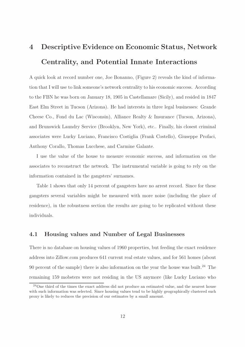
A quick look at record number one, Joe Bonanno, (Figure 2) reveals the kind of informa-

tion that I will use to link someone’s network centrality to his economic success. According

to the FBN he was born on January 18, 1905 in Castellamare (Sicily), and resided in 1847

East Elm Street in Tucson (Arizona). He had interests in three legal businesses: Grande

Cheese Co., Fond du Lac (Wisconsin), Alliance Realty & Insurance (Tucson, Arizona),

and Brunswick Laundry Service (Brooklyn, New York), etc.. Finally, his closest criminal

associates were Lucky Luciano, Francisco Costiglia (Frank Costello), Giuseppe Profaci,

Anthony Corallo, Thomas Lucchese, and Carmine Galante.

I use the value of the house to measure economic success, and information on the

associates to reconstruct the network. The instrumental variable is going to rely on the

information contained in the gangsters’ surnames.

Table 1 shows that only 14 percent of gangsters have no arrest record. Since for these

gangsters several variables might be measured with more noise (including the place of

residence), in the robustness section the results are going to be replicated without these

individuals.

4.1 Housing values and Number of Legal Businesses

There is no database on housing values of 1960 properties, but feeding the exact residence

address into Zillow.com produces 641 current real estate values, and for 561 homes (about

90 percent of the sample) there is also information on the year the house was built.24 The

remaining 159 mobsters were not residing in the US anymore (like Lucky Luciano who

24One third of the times the exact address did not produce an estimated value, and the nearest housewith such information was selected. Since housing values tend to be highly geographically clustered suchproxy is likely to reduces the precision of our estimates by a small amount.

12

had already been expelled from the country), or never lived in the US, and were based in

Italy.

Given that the distribution of the year of first arrest has almost full support within

the range 1908-1960, one can infer that the data refer to what the authorities knew in

1960.25 Records do not report any deaths and thus do not include those who were killed

before 1960, for example, Albert Anastasia boss of one of the 5 New York City families,

the Gambino family.26 So one needs to reconstruct the value of the house in 1960.

For 608 homes that are in a metropolitan statistical area I use the average housing

value in 1960 and 2000 from Gyourko et al. (forthcoming) to deflate the prices, for the

remaining 33 homes I use State level data from the Census.27

The left Panel of Figure 3 shows the relationship (truncated at the 90th percentile)

between the current and the 1960 values. Housing prices have approximately doubled

over the last 50 years, though they have increased almost 5 times in San Francisco, while

they stayed almost constant in Binghamption, Utica/Rome, or Buffalo. In the New York

MSA, where almost 300 gangsters reside prices doubled.

The 1960 5th, 10th, 25th, 50th, 75th, and 90th percentile of the housing value were 39,

50, 95, 190, 325, and 662 thousand dollars. The 95th and 99th percentiles were 1.5 and 4.7

million dollars. The right Panel of Figure 3 shows the housing value density (truncated at

the 90th percentile). The mean housing value in 1960 is 400 thousand dollar not weighting

the sample, and is smaller (379) when weighting.28

I am also going to control for the legitimate earnings opportunities, measured by the

number of legal business that gangsters own. Thirty-two percent of gangsters has no busi-

nesses, 43 percent has one, 19 percent has two, and the remaining 5 percent has 3, 4, or

25Additional evidence is the following description in Michael Russo’s file: “Recently (1960) perjuredhimself before a Grand Jury in an attempt to protect another Mafia member and narcotic trafficker.”

26His brother Anthony “Tough Tony,” instead, was killed in 1963 and is in the records.27See http://www.census.gov/hhes/www/housing/census/historic/values.html.28Table 1 shows that 10 percent of the houses found on Zillow.com were built after 1960. To control

for the fact that these houses might have a different valuation I am going to control for a dummy variableequal to one when the houses were built after 1960.

13

5 businesses. Table 2 shows the list of legal activities that at least 5 percent of members

were involved in. Weighting does little to the distribution of legal activities. Most mob-

sters owned restaurants, drugstores or were otherwise involved with the supply of food.

Real estate, casinos, car dealerships, and import-export were also common businesses.

4.2 Network-based Measures of Importance

Each criminal record contains a list of criminal associates. Figure 2 indicates, for example,

that Joe Bonanno was associated with Luciano, Costello, Profaci, Corallo, Lucchese, and

Galante. There is no evidence about how the FBN established such associations, but each

record tends to list the most important (and connected) associates.

Indirected connections are clearly more numerous, as mobsters can be listed as asso-

ciates in several records. As in Mastrobuoni and Patacchini (2012) I define two mobsters

to be connected whenever the FBN lists at least one mobster lists the other mobster in

one record. Outdegree (the number of associates listed in one file) is bounded by the

available space on a record (the maximum is 13), while indegree (the number of times

someone is listed in other records) is not. For this reason degree (the number of undirected

connections) is only weakly correlated with outdegree (37 percent), and mainly depends

on indegree.29

The number of connections is clearly the simplest but crudest way to measure the

importance of members. In recent years social network theorists proposed different cen-

trality measures to account for the importance of someone’s connections (Borgatti, 2003,

Wasserman and Faust, 1994).30

Unlike degree, which weights every contact equally, the eigenvector index weighs con-

tacts according to their centralities.31 The index takes the whole network into account

29In other words, I construct a symmetric adjacency matrix of indirected connections between mobsters’last names. Dealing with changing first names would have been a complex task.

30See also Sparrow (1991) for a discussion on centrality indices in criminal networks.31It equals the eigenvector of the largest positive eigenvalue of the adjacency matrix, the N ×N 0 and

14

(direct and indirect connections).32 The closeness index measures the average distance

between a node (a member) and all the other nodes, and its inverse is a good measure for

how isolated members are. The betweenness index measures the number of times a node is

on the shortest path between two randomly chosen nodes, measuring member’s capacity

to act like a bridge between clusters of the network, most likely Families.33 Since there is

no strong theoretical ground to prefer a particular measure, most of the following analy-

ses are going to be based on all four measures of centrality. Though with the Mafia rule

that guarantees secrecy–“No one can present himself directly to another of our friends.

There must be a third person to do it.”– gangsters who are closer to other gangsters need

fewer interlinking associates to reach a randomly chosen gangster, while gangsters with

important bridging capacities across clusters of the network have more monopoly power

in establishing such new links.

Figure 4 demonstrates that the densities of centrality measures are positively skewed.

The eigenvector index (centrality) has a density that is very similar to that of degree, while

the density of closeness is more symmetrically distributed. The density of betweenness

has the thickest right tail, meaning that very few mobsters represent bridges between

subsets of the network.

Given that the densities of the housing values as well as of the centrality measures

have such thick right tails, as in Ductor et al. (forthcoming), all these variables are taken

in logs.34 The corresponding more symmetric densities are plotted in the Online Figure

12.

The centrality measures are positively related to each other (Figure 5). Plotting log

eigenvector against log closeness generates a thick line (ρ =96 percent), which shows that

1 matrix that indicates whether gangster i and j are connected.32As first noted by Granovetter (1973), weak ties (i.e. friends of friends) are important source of

information.33The indices have been computed using UCINET 6, and with the exception of degree have been

normalized dividing each index by its maximum value.34For the betweenness centrality index, since 4.5 percent of observations have such index equal to zero,

I take the inverse hyperbolic sine transformation log(y + (y2 + 1)1/2).

15

once one penalizes the larger outliers the two centrality measures are quite similar.

But such large correlation masks a very different variability. The ratio between the

standard deviation of the log eigenvector index and the log closeness index is about 10

to 1. This has to be taken into account when interpreting standardized variations.

The correlations are lower with respect to the other two measures, especially in the

lower tail. For betweenness it seems to be driven by the fact that several mobsters,

despite having many connections, have extremely low levels of betweenness. There is

some evidence that this is driven by the hierarchies within the mafia. For about 400

mobsters I managed to reconstruct their position within the mafia, though not always

referred to their status in 1960. Underbosses and captains (caporegime), who would head

several soldiers but always within one Mafia “Family,” tend to have large degrees but

low betweenness. Counselors and bosses have the largest median betweenness measure

(about 1/2), while the medians for captains and underbosses are half that large.35 These

differences are considerably lower when using the closeness index. Counselors tend to

have large closeness and eigenvector indices, while for bosses the medians of these indices

tend to be closer to the medians of captains.

Similarly, “degree” seems to be a good measure for centrality when the number of

connections is large. When such number is small, the quality of those few connections

varies considerably, thus widening the scatter plot.

Weighting the sample the gangsters’ average number of connections mobsters drops

from 11 to 6, and more generally, the average values of all centrality measures drop when

controlling for the non-random nature of the sampling design (Table 1). While the shapes

of the distributions stay basically unchanged.

35Soldiers have a median betweenness index of about 0.18.

16

4.3 Economic Status, Network Centrality, and Potential Biases

Figure 6 shows that the unconditional expectation of log-housing value, estimated us-

ing weighted local polynomial smoothing regression, is increasing in all log-centrality

measures, and is not far from being linear. The correlation is stronger when using the

eigenvector index and the closeness index, than when using the simple degree or the

betweenness index (approximately, 20 percent versus 10 percent).

Degree is likely to be a poor measure of centrality when the connections are scarce

but valuable. Mobsters with larger betweenness indices, instead, might be more likely to

keep a low profile, after all they represent the bridge between clusters of the network,

most likely Families, and would otherwise put the whole mafia organization in peril (see

Baccara and Bar-Isaac, 2008).

For example, Bonanno tells the story about when he decided not to join Lucky Lu-

ciano’s very lucrative garment industry in New York to avoid being in the spotlights

Bonanno (1983). Such bosses might also choose to live in an unpretentious house.

There is indeed evidence of Mafia leaders’ preference for unpretentious housing. Defin-

ing leaders to be those that the FBN files describe as “leaders” or “bosses,” Table 3 shows

that such bosses tend to be more central in the network. They tend to have considerably

larger betweenness centrality than lower-ranked gangster, about 40 percent larger. Other

centrality measures differ less between bosses and lower-ranked gangsters. Despite this,

bosses tend to live in less expensive housing. This is in part driven by bosses being less

likely to be directly involved in narcotics, a very lucrative business. Later we will see that

gangsters involved in drug dealing live is houses that are about 30 percent more expensive.

Moreover, the Sicilian origin seems to influence such bias. Recently arrested bosses

who were heading the entire Sicilian mafia, Toto Riina and Bernardo Provenzano, were

living in very poor houses. Such cautious behavior seems less present in other organized

crime groups. A recently arrested boss from the Neapolitan Camorra, Francesco Schi-

17

avone, was living in a mansion, built after the house in the Hollywood movie “Scarface.”

This same pattern between the Italian region of birth and housing values is evident in

the data. The distribution of housing value for Sicilian gangsters and peninsular gang-

sters is quite different (Figure 7). Sicilian-born mobsters tend to live in considerably

cheaper housing, especially at the top of the distribution (these differences might also

be driven by housing preferences). Since Sicilian origin tends to increase the gangster’s

centrality, later in Section 5 I will test the robustness of such correlation when controlling

for such origin, and well as for additional characteristics of the gangsters. For instance,

Mastrobuoni and Patacchini (2012) show that the family composition influences the mob-

ster’s centrality, but larger families might also need larger and more expensive housing.

Even controlling for family composition and the number of legal businesses, the gang-

sters’ initial wealth, which is not recorded in the data, might represent an omitted variable.

Such wealth might be used to buy both, power inside the mafia and more expensive hous-

ing. In the next section I devise a presumably exogenous instrument that is based on

the joint spatial distribution of the gangsters’ surnames in Italy, which I will show is

moderately correlated with network centrality.

4.4 Birthplace and Potential Innate Interactions

Keeping in mind that the mafia leaders’ preference to stay in the shadow complicates the

relationship between centrality and their economic status, next I present the instrument

variable strategy used to isolate the causal effect of gangsters’ network centrality on their

housing values.

Several authors have highlighted the importance of familial, interpersonal, and com-

munal relationships in determining criminals’ success inside organized crime groups (see,

among others, Coles, 2001, Falcone and Padovani, 1991, Ianni and Reuss-Ianni, 1972).

Though most of such relationships are also likely to influence housing decisions, and thus

18

would lead to implausible exclusion restrictions. For example, larger families might be

more powerful, but need also larger housing. Marrying a gangster’s daughter is likely to

boost someone’s power inside the mafia, but might also change someone’s housing budget

directly.

Ideally, one would use mobsters’ innate characteristics, which might influence his future

chances to build connections, but are unrelated to his housing choice (other than through

the derived centrality in the network). Proximity to other mobsters represents a natural

choice. But such proximity should not be related to inherited wealth, as such wealth

might as well be used to acquire centrality. Moreover, geographic proximity based on the

place of US residence is likely to be endogenous with respect to network centrality: more

powerful mobsters might decide to live in the middle of their sphere of influence.

For these reasons I use a measure of proximity that is based on Italian and not US

residencies. Why would a measure of residency in Italy matter? Some of the mobsters

were born in Italy, but even the second generation Italian immigrants at times kept strong

links with the Italian communities their parents had left years earlier. About a quarter of

mobsters were born in Sicily, 2/3 were born outside of Italy (mostly in the US) and the

rest in other regions of Italy. Properly weighting the data, these fractions are 2/10, 7/10,

and 1/10, indicating that Sicilians tend to have more connections.

All but a handful of mobsters were of Italian origin as this was a prerequisite to become

a member.36 Table 1 shows that the average age is 48 years, which means that the average

year of birth is 1912, right in the middle of the Italian migration wave. Most mobsters

are either first or second generation immigrants.37

36The few non-Italian gangsters in the data were either French gangsters from Marseille or Corsica, orpart of the, so-called, Jewish Mafia.

37As for the remaining variables in Table 1, 80 percent of members are married (76 percent whenweighting), but only 66 percent of these have children. The overall average number of children is 1and is about 2 among members with children. 19 percent of members are married to someone whoshares her maiden name with some other member (Connected wife), though fewer are when weighting (15percent when the Markov chain weights are used). These marriages are presumably endogamous withinthe Mafia. Observe that I’m understating the percentage of marriages within the Mafia as some Mafiasurnames might be missing in the data. While it is also possible that some women might have a Mafia

19

While I do not have pre-immigration information on the exact place of origin in Italy,

for at least 30 years researchers in human biology have been exploiting the analogy between

patrilineal surname transmission and the characterization of families and communities

(Lasker, 1977).

For a number of reasons, geographic, historical, as well as social, surnames tend to

be highly geographically clustered, particularly in countries with low internal mobility

like Italy (see Allesina, 2011, Barrai et al., 1999, Zei et al., 1993).38. The geographic

distribution of surnames, called isonomy, contains a strong signal about someone’s origin.

For example, most “Mastrobuoni” are located in the Basilicata region, which is were my

father is from.39 The Bonanno surname is more widespread across the whole country,

though, again, most Bonanno families live in Sicily, and a non-negligible fraction lives in

Castellamare del Golfo, which is where Joseph Bonanno was born.40

Given that i) 30 percent of gangsters were born in Italy and later moved to the US

and even those who were born in the US were likely to keep links with Italy, and ii)

surnames tend to be geographically clustered, the way the current distribution of a given

surname overlaps with the distribution of all the other surnames represents a possible way,

possibly the only way, to measure the innate connections stemming from the gangsters’

origin country (thus unrelated to US housing prices). The main un-testable identification

assumption is that such interaction at the origin does not shape the gangsters’ housing

preferences, at least not conditional on the region of birth.

surname without being linked to any Mafia family, this is very unlikely conditional on being married toa Mafia associate. The FBN reports an average of 2 siblings per member, while the average number ofrecorded members that share the same surname is 1.58. Mobsters’ criminal career starts early. They areon average 23 years old when they end up in jail for the first time. I do not know the total number ofcrimes committed by the mobsters but I know in how many different types of crime they have apparentlybeen involved. This number varies between 0 and 9 and the average is about 2.5. Finally, about 60percent are involved in drug dealing.

38See Colantonio et al. (2003) for an overview on recent developments on the use of surnames in humanpopulation biology.

39One can try out surnames of Italian economists on the following Web sites: http://www.gens.info/or http://www.paginebianche.it/.

40Guglielmino et al. (1991) show that in Sicily genetic and cultural transmission are revealed by sur-names.

20

Looking at Figure 8 helps explaining how I construct the index. It shows the current

distribution at the zip code level of the members’ surnames, according to Italy’s phone

directory.41 42 There are 4,748 zip codes for about 60 million Italians, thus each zip

code covers a little more than 12,000 Italians, and an area of about 23 square miles, a

reasonable area within which most relationships are likely to get established. In Figure

8 each circle is proportional to the number of surnames present within each zip code.

Not surprisingly many surnames show up in Sicily, in Naples, and in Calabria. Many of

these surnames appear also in large cities that were subject to immigratory flows from the

south, like Milan, Rome, and Turin. Such migration patterns introduce some noise in the

instrument, which is why later I also compute a Potential Innate Interactions measure

that is just based on Southern regions (Campania, Molise, Calabria, Basilicata, Sicilia,

Sardegna, Puglia), with Northern regions acting as imperfect placebos, as migration might

depend on ethnic networks.

For each members’ surname I compute the probability that he shares a randomly

chosen zip code located in Italy (as a robustness check I also limit the attention to the

South) with other surnames from the list. To be more precise, the index for member i is

equal to 1,000,000 times the sum across zip codes j of the fraction of surnames of member

i present in zip codes j times the fraction of surnames of the other members (−i) in the

same zip code:

Potential innate interactions indexi = 109∑

j

#surnamei,j∑j #surnamei,j

#surname−i,j∑

j #surname−i,j

. (3)

The Potential innate interactions index (in short, interaction index) tends to be small

when the fraction of surnames i overlaps little with the fraction of all other surnames

41Only four mobsters were neither born in Italy nor in the US. For two of these mobsters (Lansky andGenese the Potential Innate Interactions index is zero).

42Ideally one would use the distribution of surnames in 1960, though previous research has shown howpersistent such distribution is (Colantonio et al., 2003).

21

−i. Dividing by the the total number of surnames i and −i takes into account that some

surnames are more frequent than others.

I can computed such index for all surnames in the data, while information about the

Italian community of origin would only be available for those born there. The average

index is equal to 36 per one million, though taking the sampling into account it drops to

26, already indicating that more connected mobsters have more interactions (see Table

1). About ten percent of the times the index is zero, either because the zip codes do not

overlap or because the surname is not in the phone directory.43

Figure 9 shows that the distribution of the interaction index. Mobsters born in Italy

tend to have more innate potential interactions than those born outside of Italy (Figure

10). Most mobsters with very large interactions were born in the Western part of Sicily

(the 10 cities of birth corresponding to the largest interaction indices are in major US

cities (Chicago, NYC, St. Luis), but also Palermo (Sicily), Cerda (Sicily), Trapani (Sicily),

Amantea (Calabria). Most of these are well-known mafia enclaves.

When measuring the interactions focussing on Southern zip codes the shape of the

bars is very similar, while when focussing on Northern zip codes (the imperfect placebo)

the interaction probabilities are considerably lower, and are lowest for Sicilians, which is

consistent with the index capturing interactions in the place of origin.

That these interactions influence the centrality measures can be seen in Figure 11

and Table 4. Correlations are between 15 (eigenvector, closeness, and degree) and 30

percent (betweenness), indicating that such initial interactions are important, though

neither necessary, nor sufficient, to reach the top positions in the organization (those

positions that generate bridges across Families). Moreover, the correlation is larger when

restricting the interactions to Southern Italy and considerably weaker when restricting

the interactions to Northern Italy.

43In the regressions I allow the zeros to have an independent effect. Moreover, ideally one would usthe mother’s surname as well, though such information is not always available.

22

Regressions in the next Section are going to assign confidence intervals to these rela-

tionships, and are going to test their robustness when further controls are added to the

model.

5 Regression Results

5.1 Evidence based on Ordinary Least Squares regressions

Starting with simple OLS regressions and with the closeness centrality measure, Table

5 shows that doubling the centrality increases the housing value by about 200 percent.44

Such large elasticities are driven by a very compressed distribution of closeness centrality.

In terms of a standard deviation increase in log closeness (0.12), the increase in housing

value is equal to 1/4.

The first column controls only for variables collected from Zillow.com, in particular

whether the housing has been built after 1960 (the year of the FBN records) and whether

such information is available. The negative coefficient on this variable is capturing that

for more expensive housing Zillow.com is more likely to collect information on the year the

house was built. Controlling for additional variables (column 2) increases somehow the

effect, while adding US State of residence fixed effects reduces them (column 3), partly

because the more influential mobsters resided in New York and New Jersey (where housing

prices tend to be high).45 Given that the State of residence measures part of the centrality

of mobsters in the remainder of the study I will not control for it, though I should add that

44Given that there is one large network, the residuals might be correlated across mobsters. Assumingthat such correlation depends on the shortest distance between pairs of gangsters the variance of theresidual of gangster i is going to be a function of the sum of all such distances dij over j. In particular,σi =

∑j σij(dij). Approximating such variance with either a linear function or an exponential function

in average distances (the inverse of closeness) one always rejects that distance influences the squaredresiduals, and thus the correlations across mobsters (see appendix Table 9). Nevertheless, in all regressionsthe standard errors are clustered at the surname level, which is the level at which the centrality measuresare calculated.

45Measurement error might also be co-responsible for such drop.

23

the instrument that is going to be used later in Section 5.2 is, by construction, unrelated

to the State of residence (other than through connections).

The last two columns show that similar results are found when using closeness in levels

rather than in logs, though in such case the predictive power of centrality drops slightly. As

for the log, a standard deviation increase in closeness centrality (8.27) increases housing

values by about a quarter.

Before showing the results for other centrality measures, let me briefly discuss the coef-

ficients on the other regressors. Gangsters born in Italy, in particular those born in Sicily

tend to live in cheaper housing, which might either be due to housing preferences or to a

more pronounced avoidance to attract attention (though the effects are not significantly

different from 0).46

Age at first arrest, which might represent a (negative) measure of career experience

within the organization tends to be negatively related to housing values, meaning that

earlier arrests tend to be related to increased housing values. Not just experience, but also

being involved with drug dealing seems to be related to higher housing values, though

the coefficient stops being significant once state of residence effects are added to the

regression (indicating that the drug dealing business used to be geographically clustered).

The number of legal businesses tend to be positively associated with housing values, which

is not surprising.

Going to back to the centrality measures, in Table 6 I substitute closeness centrality

with the other measures, with and without controlling for additional regressors. A quick

look at the R-squared reveals that closeness centrality is the strongest predictor of housing

value. This is coherent with the first rule of the Mafia, which states that only interlinking

affiliates, for example B in a network A-B-C, have the power to introduce a direct link

between A and B. Mobsters who are on average closer to all other mobsters will thus need

46Appendix Table 10 shows that the place of birth, while influencing the housing value, does notintroduce heterogeneity in the effect of centrality.

24

fewer interlinking associates to establish new connections.

In the absence of a network formation theory for such an illegal and secret organization,

I will emphasize the results based on the centrality with the highest predictive power,

namely closeness centrality.

Eigenvector centrality has similar predictive power, which is not surprising given how

strongly correlated the two measures are.47

The elasticity is larger for closeness centrality only because its variation is about 10

times smaller than the one of eigenvector centrality. One standard deviation increase in

log-closeness centrality has about the same impact on housing value as a one standard

deviation increase in log eigenvector centrality.

The coefficient on degree, instead, has relatively larger standard errors, and a standard

deviation increase in log degree increases housing value by about 11 percent; but, in line

with what emerged in Figure 6, the flattest relationship is the one between log housing

value and log betweenness centrality. Statistically speaking, the slope is 0.

Given that innate interactions have their strongest influence on such centrality, this is

quite unfortunate. Especially because, as argued before, such bias cannot be eliminated.

All the regressions use the weighting strategy developed earlier on, but the results based

on unweighted regressions can be seen in the Online Table 11. The next Section will show

this more formally, and will also show whether the instrument is strong enough to be used

for the other centrality measures.

5.2 Evidence based on Instrumental Variable regressions

As previously discussed, for a number of reasons ordinary least squared coefficients on

centrality measures might be biased. Figure 11 showed that potential innate interactions

influence the gangsters’ network centrality. Table 7 presents the first stage and second

47This indicates that the underlying network formation model might not be far from those that havealready been developed (Ballester et al., 2006).

25

stage regressions in a compact form, focussing on the instruments and on the endogenous

variable, while appendix Tables 12 and 13 show all the coefficients.

Having no potential innate connections is allowed to have its own influence on central-

ity. All centrality measures are positively correlated with the potential, but the coefficient

is significant only for closeness and betweenness centralities.

The instrument is rather weak. In particular, for closeness and betweenness central-

ity the F-statistic for the excluded instruments is around 2 when considering the joint

significance of interactions and zero interactions (otherwise it is close to 4). While there

are no Montecarlo simulations to determine the bias for clustered standard errors, we

should take into account that the estimates are likely to be biased toward OLS. Later

I will try to increase the strength of the instrument by i) focussing on the 86 percent

of gangsters how have been arrested at least once, and for whom all variable are more

likely to be measured with precision, and ii) using a measure of interactions based on

just Southern Italy, which has been shown is more strongly related to centrality. This is

probably because over the last 50 years in the South, particulary when compared to the

North, intranational immigration figures have been small.

Instrumenting the centrality measures the coefficients on closeness, eigenvector, as well

as on degree centrality tend to be almost 4 times as large as the OLS equivalents, meaning

that a standard deviation increase in either closeness or eigenvector centrality doubles

the housing value. As in the OLS case, betweenness does not appear to be significantly

different from 0, confirming that the gangsters with large bridging capacity tend to keep

a lower profile, no matter whether the centrality has been reached exploiting potential

innate connections or not.

But overall the relative precision of the estimates tends to be smaller than for the

OLS regressions, which is in part due to the instrument’s weakness. Indeed, the standard

errors are so large that endogeneity is generally rejected (although at p-values that are

26

not too far from 10 percent).

Table 8 performs several robustness checks, and two are aimed at increasing the

strength of the instrument. In columns 1 and 2 I restrict the analysis to gangsters who

have at least one arrest record. About 85 percent of gangsters have an arrest record, and

for these gangsters all the collected information, in particular, the surname, the place

of residence, as well as the connections are more likely to be measured with increased

accuracy (though the sample is a more selected one).

In particular, surnames, which represent the core information for the instrumental vari-

able strategy, are not easily measured inside the Mafia. Gangsters are typically known

by their nickname. Some of the aliases for gangsters mentioned before were: Don Vi-

tone, The Old Man (Vito Genovese); Francisco Castiglia, Frank Costello, Frank Saverio,

Saveria (Francisco Costiglia); Joe Bananas, Joe Bononno, Joe Bonnano, Joe Bouventre

(Joseph Bonanno), Joe Proface (Giuseppe Profaci); Carlo Gambrino, Carlo Gambrieno,

Don Carlo (Carlo Gambino). Knowing the exact name is clearly important to reconstruct

its geographical distribution in Italy, and for arrested gangsters such information is clearly

more precise.

The OLS coefficient and IV coefficients in columns 1 and 2 are indeed slightly larger,

and, based on the Kleibergen-Paap rk Wald F statistic, the instrument becomes more

than twice as powerful.

Column 5, where only the distribution in Southern Italian zip codes are used to mea-

sure interactions has a similar influence on the Kleibergen-Paap rk Wald F statistic, in-

dicating that migration patterns to the major cities in Central and Northern Italy might

have introduced some noise in the instrument.48

Columns 3 and 4 test the robustness of the results when getting rid of the zero in-

teraction dummy (thus assuming continuity and linearity at 0), and when allowing the

48The same conclusions can be drawn looking at the reduced form regressions, shown in appendix Table14.

27

instrument to have non-linear effects on log closeness. None of these changes alters the

results. Finally, in the last column I add a variable that is clearly endogenous, whether

the mobster is married to a “connected” wife, meaning a wife whose maiden name is also

the surname of another mobster in the data.

These marriages tended to be arranged for strategic reasons, and would allow gangsters

to gain additional power (connections) as well as wealth. Adding this variable increases

the OLS estimates while keeping the 2SLS estimate almost unchanged, suggesting that

omitted variables (which the instrument takes care of) are indeed biasing the OLS estimate

toward zero.49

6 Concluding remarks

This paper estimates how in 1960 inside the Italian-American Mafia network centrality

influenced economic prosperity, measured based on reconstructed housing values, dealing

with the non-random sampling design of such law-enforcement data. .

In the overground world connections, and their whole geometry, have been shown to be

related to a variety of economic outcomes. In the underground world such connections are

presumably even more important, and yet evidence of this is mainly based on ethnographic

studies.

Moreover, even in the overground world researchers have rarely gone beyond just

documenting correlations, as networks tend to emerge endogenously out of complicated

bilateral and multilateral decision processes. Social scientists have been able to exploit

the geometry of the network to develop identification strategies for direct connections

(peer effects), but not yet for measures of how central an individual is inside the network.

Alternatively, one has to either i) use a two-step estimation procedure where the first

step models the endogenous network formation (which is easily prone to model mis-

49The potential endogeneity of such marriage hinders stronger statements.

28

specification), or use an instrumental variable approach.

But instrument for networks with reasonable exclusion restrictions are in short supply.

Any characteristic that determines someone’s position inside his/her network is also likely

to directly influence a multitude of other outcomes. In the Mafia, for example, family

relationships, wealth, place of birth, etc. might help securing a centrality in the network,

but could easily be related to the demand for housing.

For migrants with strong ethnic identities, instruments naturally evolve from shocks

that happen in the country of origin and are thus less likely to influence economic outcomes

in the country of destination. Munshi (2003) uses rainfall in Mexico to instrument for

the network size of Mexican immigrants to study how such size influences labor market

outcomes. Similarly, this paper instruments individual centrality measures using the

potential exposure to connections in the gangster’s place of origin. In the absence of pre-

immigration data I use the informational content of surnames, called isonomy, to measure

such place.

On the one hand, mobsters who were on average closer to their peers, and who had

more connections and more connections to more connected peers tend to live in more

expensive housing. This is consistent with the importance of interconnection capacity in

a secret society where unconnected mobsters need a common connection to generate a

direct link.

On the other hand, mobsters who act as bridges across clusters of the larger network

(given what is know about the Mafia these could be called Mafia Families, or “Manda-

menti”) tend to keep a lower profile, preferring less expensive housing. The evidence

suggests that these tend to be the more important bosses, those who most likely form the

governing body of the Mafia (la Commissione). In line with Bonnano’s autobiography

such bosses were less likely to be directly involved in the narcotics businesses, which might

be part of the same attention avoidance strategy (Bonanno, 1983).

29

Despite having to use i) the informational content of surnames to measures the gang-

sters’ roots, ii) today’s housing values to reconstruct the 1960 housing values, iii) a sub-

sample of the entire network, the instrumental evidence suggests that a one-standard

deviation increase in closeness centrality doubles the gangster’s housing value. Given

that such effects appear to be bound to be close to zero for extremely central gangsters

(the information hubs, or bridges) the effects on true economic outcomes, which might

not be simply measured with classical errors (wealth in the hands of figureheads might

be increasing in centrality) are likely to be even larger.

Finally, while data restrictions prevent researchers from performing similar analyses

based on more recent organized crime networks, this might hopefully change in the near

future. Understanding how central figures grow up inside criminal networks is fundamen-

tal to the design of targeted law enforcement strategies.

30

References

MAFIA: The Government’s Secret File on Organized Crime. By the United States Trea-

sury Department, Bureau of Narcotics. HarperCollins Publishers, 2007.

Howard Abadinsky. Organized Crime. Wadsworth Publishing, 1990.

Vivi Alatas, Abhijit Banerjee, Rema Hanna Arun G. Chandrasekhar, and Benjamin A.

Olken. Network Structure and the Aggregation of Information: Theory and Evidence

from Indonesia. 2012.

Stefano Allesina. Measuring nepotism through shared last names: the case of italian

academia. PLoS one, 6(8):e21160, 2011.

Manuela Angelucci and Giacomo De Giorgi. Indirect effects of an aid program: How do

cash transfers affect ineligibles’ consumption? The American Economic Review, pages

486–508, 2009.

Mariagiovanni Baccara and Heski Bar-Isaac. How to Organize Crime. Review of Economic

Studies, 75(4):1039–1067, 2008.

Wayne E. Baker and Robert R. Faulkner. The Social Organization of Conspiracy: Illegal

Networks in the Heavy Electrical Equipment Industry. American Sociological Review,

58(6):pp. 837–860, 1993.

Coralio Ballester, Yves Zenou, and Antoni Calvo-Armengol. Who’s who in networks.

wanted: The key player. Econometrica, 74(5):1403–1417, 09 2006.

Coralio Ballester, Yves Zenou, and Antoni Calvo-Armengol. Delinquent networks. Journal

of the European Economic Association, 8(1):34–61, 2010.

31

Oriana Bandiera. Land reform, the market for protection, and the origins of the Sicilian

mafia: theory and evidence. Journal of Law, Economics, and Organization, 19(1):218,

2003.

Oriana Bandiera and Imran Rasul. Social networks and technology adoption in northern

mozambique*. The Economic Journal, 116(514):869–902, 2006.

Oriana Bandiera, Iwan Barankay, and Imran Rasul. Social connections and incentives in

the workplace: Evidence from personnel data. Econometrica, 77(4):1047–1094, 2009.

Abhijit Banerjee, Abhijit Banerjee, Arun G Chandrasekhar, Esther Duflo, and Matthew O

Jackson. The Diffusion of Microfinance. Science, 341(1236498), 2013.

I Barrai, A Rodriguez-Larralde, E Mamolini, and C Scapoli. Isonymy and isolation by

distance in italy. Human Biology, pages 947–961, 1999.

Patrick Bayer, Stephen Ross, and Giorgio Topa. Place of work and place of residence:

Informal hiring networks and labor market outcomes. Journal of Political Economy,

116:1150–1196, 2008.

Patrick Bayer, Randi Hjalmarsson, and David Pozen. Building criminal capital behind

bars: Peer effects in juvenile corrections. The Quarterly Journal of Economics, 124(1):

105–147, 2009.

Marianne Bertrand, Erzo FP Luttmer, and Sendhil Mullainathan. Network effects and

welfare cultures. The Quarterly Journal of Economics, 115(3):1019–1055, 2000.

Lawrence E Blume, William A Brock, Steven N Durlauf, and Rajshri Jayaraman. Linear

Social Network Models. 2012.

Joseph Bonanno. A Man of Honor: The Autobiography of Joseph Bonanno. St. Martin’s,

1983.

32

Steve P. Borgatti. The Key Player Problem, pages 241–252. R. Breiger, K. Carley and P.

Pattison, Committee on Human Factors, National Research Council, 2003.

P. Buonanno, R. Durante, G. Prarolo, and P. Vanin. Poor institutions, rich mines: Re-

source curse and the origins of the sicilian mafia. Working Papers wp844, Dipartimento

Scienze Economiche, Universita’ di Bologna, September 2012.

Antoni Calvo-Armengol, Eleonora Patacchini, and Yves Zenou. Peer effects and social

networks in education. The Review of Economic Studies, 76(4):1239–1267, 2009.

Sonia Colantonio, Gabriel Ward Lasker, Bernice A Kaplan, and Vicente Fuster. Use of

surname models in human population biology: a review of recent developments. Human

Biology, 75(6):785–807, 2003.

Nigel Coles. It’s Not What You Know-It’s Who You Know That Counts. Analysing

Serious Crime Groups as Social Networks. British Journal of Criminology, 41(4):580,

2001.

David Critchley. The Origin of Organized Crime in America: The New York City Mafia,

1891–1931. Routledge, 2009.

Giacomo De Giorgi, Michele Pellizzari, and Silvia Redaelli. Identification of social interac-

tions through partially overlapping peer groups. American Economic Journal: Applied

Economics, pages 241–275, 2010.

Scott H. Decker, Tim Bynum, and Deborah Weisel. A Tale of two Cities: Gangs as

Organized Crime Groups. Justice Quarterly, 15(3):395–425, 1998.

Arcangelo Dimico, Alessia Isopi, and Ola Olsson. Origins of the sicilian mafia: The market

for lemons. Discussion Papers 12/01, University of Nottingham, CREDIT, 2012.

33

Francesco Drago and Roberto Galbiati. Indirect effects of a policy altering criminal

behavior: Evidence from the italian prison experiment. American Economic Journal:

Applied Economics, 4(2):199–218, April 2012.

Lorenzo Ductor, Marcel Fafchamps, Sanjeev Goyal, and Marco J van der Leij. Social

networks and research output. Review of Economics and Statistics, forthcoming.

Esther Duflo and Emmanuel Saez. The role of information and social interactions in

retirement plan decisions: Evidence from a randomized experiment. The Quarterly

Journal of Economics, 118(3):815–842, 2003.

Marcel Fafchamps, Ana Vaz, and Pedro C Vicente. Voting and Peer Effects : Experimental

Evidence from Mozambique. 2013.

Giovanni Falcone and Marcelle Padovani. Cose di Cosa Nostra. Rizzoli, 1991.

Gianluca Fiorentini and Sam Peltzman. The Economics of Organised Crime. Cambridge

University Press, 1997.

Diego Gambetta. The Sicilian Mafia: the business of private protection. Harvard Univ

Press, 1996.

Nuno Garoupa. Optimal law enforcement and criminal organization. Journal of Economic

Behavior & Organization, 63(3):461–474, July 2007.

Edward L Glaeser, Bruce Sacerdote, and Jose A Scheinkman. Crime and social interac-

tions. The Quarterly Journal of Economics, 111(2):507–548, 1996.

Allen C Goodman. An econometric model of housing price, permanent income, tenure

choice, and housing demand. Journal of Urban Economics, 23(3):327–353, 1988.

Martin A. Gosch and Richard Hammer. The Last Testament of Lucky Luciano. Little,

Brown, 1975.

34

Sanjeev Goyal. Connections: An Introduction to the Economics of Networks. Princeton:

Princeton University Press, 2007.

Mark S. Granovetter. The strength of weak ties. American Journal of Sociology, 78:

1360–1380., 1973.

CR Guglielmino, G Zei, and LL Cavalli-Sforza. Genetic and cultural transmission in sicily

as revealed by names and surnames. Human biology, pages 607–627, 1991.

Luigi Guiso, Paola Sapienza, and Luigi Zingales. Does Culture Affect Economic Out-

comes? The Journal of Economic Perspectives, 20(2):23–48, 2006.

Joseph Gyourko, Christopher Mayer, and Todd Sinai. Superstar cities. American Eco-

nomic Journal: Economic Policy, forthcoming.

Dana L Haynie. Delinquent peers revisited: Does network structure matter? 1. American

journal of sociology, 106(4):1013–1057, 2001.

Douglas D. Heckathorn. Respondent-driven sampling: a new approach to the study of

hidden populations. Social problems, pages 174–199, 1997.

Francis A.J. Ianni and Elisabeth Reuss-Ianni. A Family Business: Kinship and Social

Control in Organized Crime. Russell Sage Foundation, 1972.

Matthew O. Jackson. Social and Economic Networks. Princeton: Princeton University

Press., 2008.

James B. Jacobs and Lauryn P. Gouldin. Cosa nostra: The final chapter? Crime and

Justice, 25:pp. 129–189, 1999.

Valdis E. Krebs. Mapping Networks of Terrorist Cells. Connections, 24(3):43–52, 2002.

Vimal Kumar and Stergios Skaperdas. Criminal Law and Economics, chapter On The

Economics of Organized Crime. Edward Elgar Pub, 2009.

35

Gabriel W Lasker. A coefficient of relationship by isonymy: a method for estimating the

genetic relationship between populations. Human Biology, pages 489–493, 1977.

Steven D. Levitt and Sudhir Alladi Venkatesh. An economic analysis of a drug-selling

gang’s finances. The Quarterly Journal of Economics, 115(3):755–789, August 2000.

Salvatore Lupo. Quando la Mafia Trovo l’America. Einaudi, 2009.

Peter Maas. The Valachi Papers. Putnam, New York, 1968.

Alexandre Mas and Enrico Moretti. Peers at work. The American Economic Review, 99

(1):112–145, 2009.

Giovanni Mastrobuoni and Eleonora Patacchini. Organized Crime Networks: an Appli-

cation of Network Analysis Techniques to the American Mafia. Review of Network

Economics, 3, September 2012.

Jean Marie McGloin. Policy And Intervention Considerations of a Network Analysis of

Street Gangs. Criminology & Public Policy, 4(3):607–635, 2005.

John C. McWilliams. The Protectors: Harry J. Anslinger and the Federal Bureau of

Narcotics, 1930-1962. Univ of Delaware Press, 1990.

James D Montgomery. Social networks and labor-market outcomes: Toward an economic

analysis. The American Economic Review, 81(5):1408–1418, 1991.

Carlo Morselli. Career opportunities and network-based privileges in the Cosa Nostra.

Crime, Law and Social Change, 39(4):383–418, 2003.

K. Munshi. Networks in the Modern Economy: Mexican Migrants in the US Labor

Market. Quarterly Journal of Economics, 118(2):549–599, 2003.

Mangai Natarajan. Understanding the Structure of a Drug Trafficking Organization: A

Conversational Analysis. Crime Prevention Studies, 11:273–298, 2000.

36

Mangai Natarajan. Understanding the Structure of a Large Heroin Distribution Network:

A Quantitative Analysis of Qualitative Data. Journal of Quantitative Criminology, 22

(2):171–192, 2006.

Eleonora Patacchini and Yves Zenou. The strength of weak ties in crime. European

Economic Review, 52:209–236, 2008.

Eleonora Patacchini and Yves Zenou. Juvenile delinquency and conformism. Journal of

Law, Economics & Organization, 28(1):1–31, 2012.

Peter Reuter. Disorganized Crime: the Economics of the Visible Hand. MIT press, 1983.

Peter Reuter. Handbook of organized crime in the United States, chapter Research on

American Organized Crime. Greenwood Press, Westport, CT, 1994.

Jerzy Sarnecki. Delinquent Networks in Sweden. Journal of Quantitative Criminology, 6

(1):31–50, 1990. ISSN 0748-4518.

Jerzy Sarnecki. Delinquent Networks: Youth Co-offending in Stockholm. Cambridge Univ

Pr, 2001. ISBN 0521802393.

Friedrich Schneider and Dominik H. Enste. Shadow economies: Size, causes, and conse-

quences. Journal of Economic Literature, 38(1):77–114, March 2000.

Sibel Sirakaya. Recidivism and social interactions. Journal of the American Statistical

Association, 101(475):863–877, 2006.

Malcolm K. Sparrow. The Application of Network Analysis to Criminal Intelligence: an

Assessment of the Prospects. Social Networks, 13(3):251 – 274, 1991.

F. Vega-Redondo. Complex Social Networks. Econometric Society Monograph Series.

Cambridge: Cambridge University Press., 2007.

37

John R. Wagley. Transnational Organized Crime: Principal Threats and US Responses.

Congressional Research Service Report for Congress RL33335, March 2006.

Stanley Wasserman and Katherine Faust. Social Network Analysis. Methods and Appli-

cations. Cambridge: Cambridge university press edition, 1994.

Phil Williams. Transnational Criminal Networks. Networks and netwars: the future of

terror, crime, and militancy, page 61, 2001.

George Wolf and Joseph DiMona. Frank Costello: Prime Minister of the Underworld.

Morrow, 1974.

Gianna Zei, Guido Barbujani, Antonella Lisa, Ornella Fiorani, Paolo Menozzi, Enzo Siri,

and Luigi Luca Cavalli-Sforza. Barriers to gene flow estimated by surname distribution

in italy. Annals of Human Genetics, 57(2):123–140, 1993.

38

Figure 1: Surveillance pictures of Nick Giso in 1980, and Sammy Gravano in 1988

39

Figure 2: Record Number One: Joe Bonanno

40

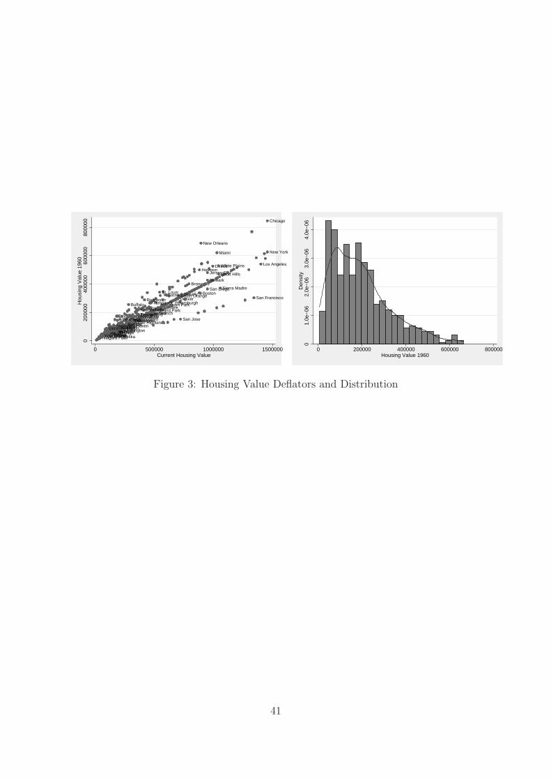
Ansonia

Atlantic Highlands

Auburn−Opelika

BaltimoreBaton Rouge

Binghamton

Boston

Bronxville

Buffalo

Burlington

Centereach

Chicago

Cleveland

Coalinga

Dallas

Denver

Des Moines

Detroit

Fanwood

Florham Park

GalvestonHazleton

Highland Park

Houston

Iselin

Jersey City

Kansas City

Las VegasLewiston

Long Branch

Los Angeles

Medford

Miami

Monroe

New HavenNew Kensington

New Milford

New Orleans

New York

Newark

Niagara FallsOmaha

PassaicPhiladelphiaPittsburgh

Port Byron

Providence

Pueblo

Rochester

San Diego

San Francisco

San Jose

Scranton

Short Hills

Sierra Madre

Somerset

South Orange

Springfield

St. Louis

Tampa−St. Petersburgh

Teaneck

Tenafly

Trinidad

Tucson

Utica−Rome

Valhalla

Vallejo

White Plains

Youngstown

020

0000

4000

0060

0000

8000

00H

ousi

ng V

alue

196

0

0 500000 1000000 1500000Current Housing Value

01.

0e−

062.

0e−

063.

0e−

064.

0e−

06D

ensi

ty

0 200000 400000 600000 800000Housing Value 1960

Figure 3: Housing Value Deflators and Distribution

41

0.0

2.0

4.0

6.0

8D

ensi

ty

0 20 40 60Eigenvector

0.0

2.0

4.0

6.0

8.1

Den

sity

0 10 20 30 40Degree

0.0

1.0

2.0

3.0

4.0

5D

ensi

ty

50 60 70 80 90 100Closeness

0.1

.2.3

.4D

ensi

ty

0 10 20 30Betweenness

Figure 4: Densities of Centrality Indices

Notes: The density shown excludes the top 1 percent of the distribution.

42

logDegree

logEigenvector

logCloseness

logBetweenness

0

2

4

0 2 4

−5

0

5

−5 0 5

3

3.2

3.4

3.6

3 3.2 3.4 3.60

1

2

3

0 1 2 3

Figure 5: Relationship Between Log-centrality Indices

Notes: The density shown excludes the top 1 percent of the distribution.

43

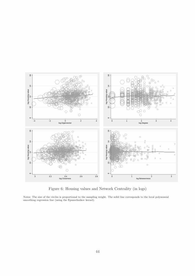
810

1214

16lo

g H

ousi

ng v

alue

−4 −2 0 2 4log Eigenvector

810

1214

16lo

g H

ousi

ng v

alue

0 1 2 3 4log Degree

810

1214

16lo

g H

ousi

ng v

alue

3 3.2 3.4 3.6 3.8log Closeness

810

1214

16lo

g H

ousi

ng v

alue

0 1 2 3log Betweenness

Figure 6: Housing values and Network Centrality (in logs)

Notes: The size of the circles is proportional to the sampling weight. The solid line corresponds to the local polynomialsmoothing regression line (using the Epanechnikov kernel).

44

050

0000

1.0e

+06

1.5e

+06

2.0e

+06

Italy, not Sicily U.S. Sicily

p 25 of value p 50 of valuep 75 of value p 95 of valuemean of value

Figure 7: Distribution of Housing Values by Region of Birth

45

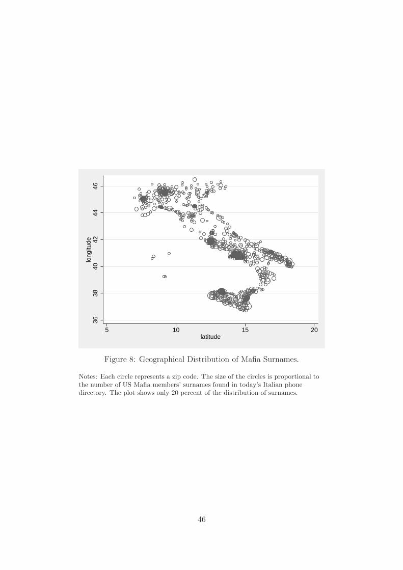
3638

4042

4446

long

itude

5 10 15 20latitude

Figure 8: Geographical Distribution of Mafia Surnames.

Notes: Each circle represents a zip code. The size of the circles is proportional tothe number of US Mafia members’ surnames found in today’s Italian phonedirectory. The plot shows only 20 percent of the distribution of surnames.

46

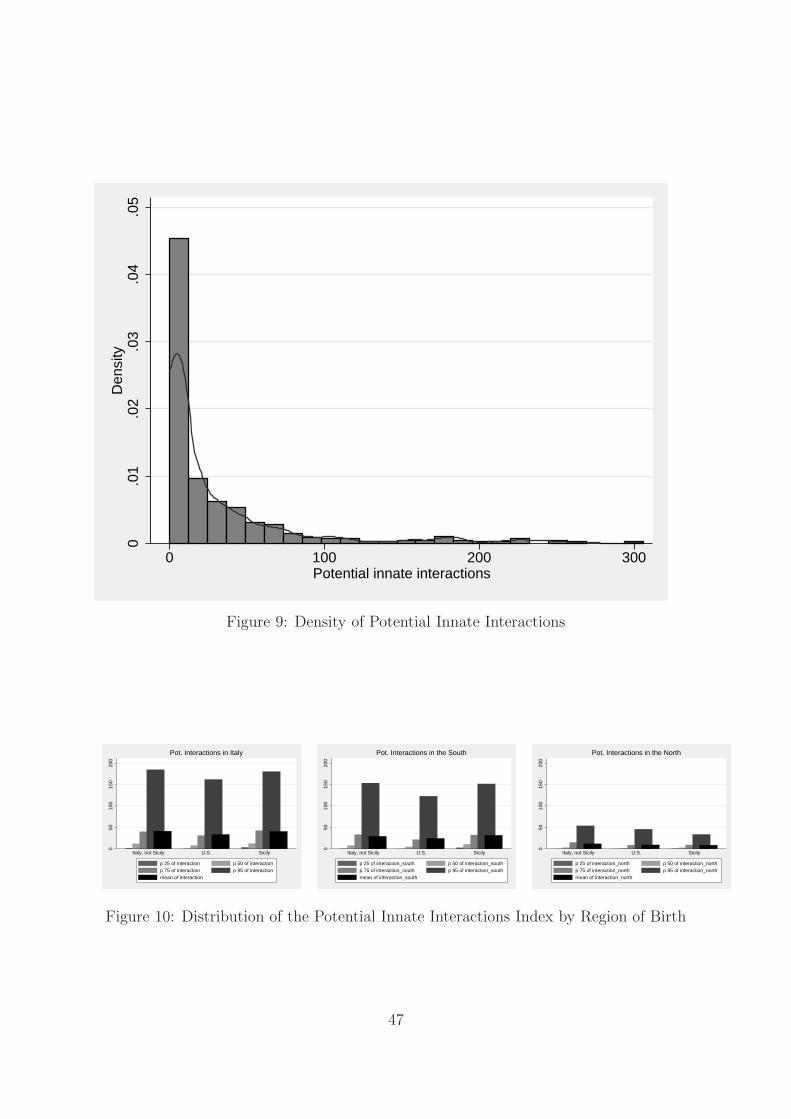
0.0

1.0

2.0

3.0

4.0

5D

ensi

ty

0 100 200 300Potential innate interactions

Figure 9: Density of Potential Innate Interactions

050

100

150

200

Italy, not Sicily U.S. Sicily

Pot. Interactions in Italy

p 25 of interaction p 50 of interactionp 75 of interaction p 95 of interactionmean of interaction

050

100

150

200

Italy, not Sicily U.S. Sicily

Pot. Interactions in the South

p 25 of interaction_south p 50 of interaction_southp 75 of interaction_south p 95 of interaction_southmean of interaction_south

050

100

150

200

Italy, not Sicily U.S. Sicily

Pot. Interactions in the North

p 25 of interaction_north p 50 of interaction_northp 75 of interaction_north p 95 of interaction_northmean of interaction_north

Figure 10: Distribution of the Potential Innate Interactions Index by Region of Birth

47

−4

−2

02

4lo

g E

igen

vect

or

0 50 100 150Potential innate interactions

01

23

4lo

g D

egre

e

0 50 100 150Potential innate interactions

33.

23.

43.

63.

8lo

g C

lose

ness

0 50 100 150Potential innate interactions

01

23

log

Bet

wee

nnes

s

0 50 100 150Potential innate interactions

Figure 11: Network Centrality and Potential Innate Interactions Index (in logs)

Notes: The size of the circles is proportional to the sampling weight. The solid line corresponds to the local polynomialsmoothing regression line (using the Epanechnikov kernel).

48

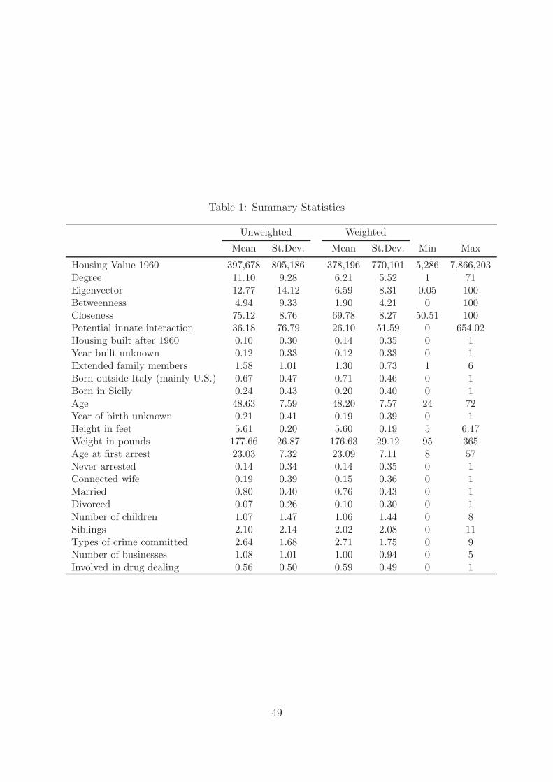
Table 1: Summary Statistics

Unweighted Weighted

Mean St.Dev. Mean St.Dev. Min Max

Housing Value 1960 397,678 805,186 378,196 770,101 5,286 7,866,203Degree 11.10 9.28 6.21 5.52 1 71Eigenvector 12.77 14.12 6.59 8.31 0.05 100Betweenness 4.94 9.33 1.90 4.21 0 100Closeness 75.12 8.76 69.78 8.27 50.51 100Potential innate interaction 36.18 76.79 26.10 51.59 0 654.02Housing built after 1960 0.10 0.30 0.14 0.35 0 1Year built unknown 0.12 0.33 0.12 0.33 0 1Extended family members 1.58 1.01 1.30 0.73 1 6Born outside Italy (mainly U.S.) 0.67 0.47 0.71 0.46 0 1Born in Sicily 0.24 0.43 0.20 0.40 0 1Age 48.63 7.59 48.20 7.57 24 72Year of birth unknown 0.21 0.41 0.19 0.39 0 1Height in feet 5.61 0.20 5.60 0.19 5 6.17Weight in pounds 177.66 26.87 176.63 29.12 95 365Age at first arrest 23.03 7.32 23.09 7.11 8 57Never arrested 0.14 0.34 0.14 0.35 0 1Connected wife 0.19 0.39 0.15 0.36 0 1Married 0.80 0.40 0.76 0.43 0 1Divorced 0.07 0.26 0.10 0.30 0 1Number of children 1.07 1.47 1.06 1.44 0 8Siblings 2.10 2.14 2.02 2.08 0 11Types of crime committed 2.64 1.68 2.71 1.75 0 9Number of businesses 1.08 1.01 1.00 0.94 0 5Involved in drug dealing 0.56 0.50 0.59 0.49 0 1

49

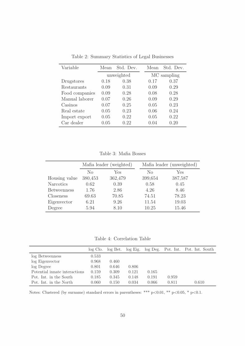
Table 2: Summary Statistics of Legal Businesses

Variable Mean Std. Dev. Mean Std. Dev.

unweighted MC samplingDrugstores 0.18 0.38 0.17 0.37Restaurants 0.09 0.31 0.09 0.29Food companies 0.09 0.28 0.08 0.28Manual laborer 0.07 0.26 0.09 0.29Casinos 0.07 0.25 0.05 0.23Real estate 0.05 0.23 0.06 0.24Import export 0.05 0.22 0.05 0.22Car dealer 0.05 0.22 0.04 0.20

Table 3: Mafia Bosses

Mafia leader (weighted) Mafia leader (unweighted)

No Yes No YesHousing value 380,453 362,479 399,654 387,587Narcotics 0.62 0.39 0.58 0.45Betweenness 1.76 2.86 4.26 8.46Closeness 69.63 70.85 74.51 78.23Eigenvector 6.21 9.26 11.54 19.03Degree 5.94 8.10 10.25 15.46

Table 4: Correlation Table

log Clo. log Bet. log Eig. log Deg. Pot. Int. Pot. Int. South

log Betweenness 0.533log Eigenvector 0.968 0.460log Degree 0.801 0.646 0.806Potential innate interactions 0.159 0.309 0.121 0.165Pot. Int. in the South 0.185 0.345 0.148 0.191 0.959Pot. Int. in the North 0.060 0.150 0.034 0.066 0.811 0.610

Notes: Clustered (by surname) standard errors in parentheses: *** p<0.01, ** p<0.05, * p<0.1.

50

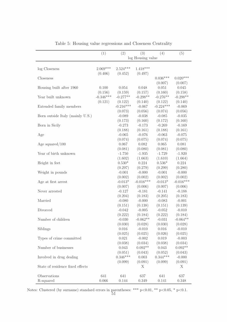
Table 5: Housing value regressions and Closeness Centrality

(1) (2) (3) (4) (5)log Housing value

log Closeness 2.069*** 2.524*** 1.418***(0.406) (0.452) (0.497)

Closeness 0.036*** 0.020***(0.007) (0.007)

Housing built after 1960 0.100 0.054 0.048 0.051 0.045(0.156) (0.159) (0.157) (0.160) (0.158)

Year built unknown -0.346*** -0.277** -0.298** -0.276** -0.298**(0.121) (0.122) (0.140) (0.122) (0.140)

Extended family members -0.216*** -0.067 -0.224*** -0.069(0.073) (0.056) (0.074) (0.056)

Born outside Italy (mainly U.S.) -0.089 -0.038 -0.085 -0.035(0.173) (0.160) (0.172) (0.160)

Born in Sicily -0.273 -0.173 -0.269 -0.169(0.188) (0.161) (0.188) (0.161)

Age -0.065 -0.076 -0.063 -0.075(0.074) (0.075) (0.074) (0.075)

Age squared/100 0.067 0.082 0.065 0.081(0.081) (0.080) (0.081) (0.080)

Year of birth unknown -1.750 -1.935 -1.729 -1.920(1.602) (1.663) (1.610) (1.664)

Height in feet 0.530* 0.224 0.536* 0.224(0.297) (0.279) (0.299) (0.280)

Weight in pounds -0.001 -0.000 -0.001 -0.000(0.002) (0.002) (0.002) (0.002)

Age at first arrest -0.013* -0.016*** -0.013* -0.016***(0.007) (0.006) (0.007) (0.006)

Never arrested -0.127 -0.181 -0.141 -0.188(0.204) (0.183) (0.205) (0.183)

Married -0.080 -0.000 -0.083 -0.001(0.151) (0.138) (0.151) (0.139)

Divorced -0.042 -0.005 -0.052 -0.010(0.222) (0.184) (0.222) (0.184)

Number of children -0.030 -0.062** -0.031 -0.064**(0.030) (0.028) (0.030) (0.028)

Siblings 0.016 -0.010 0.016 -0.010(0.025) (0.025) (0.026) (0.025)

Types of crime committed 0.021 -0.002 0.019 -0.003(0.038) (0.034) (0.038) (0.034)

Number of businesses 0.043 0.092** 0.043 0.092**(0.051) (0.043) (0.052) (0.043)

Involved in drug dealing 0.346*** 0.003 0.344*** -0.000(0.099) (0.091) (0.099) (0.091)

State of residence fixed effects X X

Observations 641 641 637 641 637R-squared 0.066 0.144 0.349 0.141 0.348

Notes: Clustered (by surname) standard errors in parentheses: *** p<0.01, ** p<0.05, * p<0.1.51

Table 6: Housing value regressions with other centrality measures

(1) (2) (3) (4) (5) (6)log Housing Value

log Eigenvector 0.184*** 0.218***(0.040) (0.043)

log Degree 0.148** 0.220***(0.068) (0.083)

log Betweenness -0.085 0.036(0.115) (0.158)

Other Xs X X XObservations 641 641 641 641 641 641R-squared 0.062 0.136 0.025 0.098 0.014 0.076

Notes: All regressions control for the housing variables. The additional regressors regressors (“OtherXs”) are the same as in Table 5. Clustered (by surname) standard errors in parentheses: *** p<0.01, **p<0.05, * p<0.1.

52

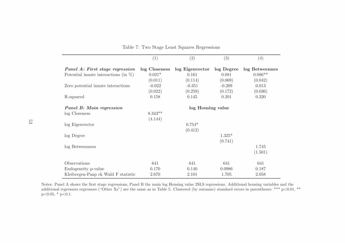
Table 7: Two Stage Least Squares Regressions

(1) (2) (3) (4)

Panel A: First stage regression log Closeness log Eigenvector log Degree log Betweennes

Potential innate interactions (in %) 0.021* 0.161 0.081 0.086**(0.011) (0.114) (0.069) (0.042)

Zero potential innate interactions -0.022 -0.351 -0.209 0.013(0.022) (0.259) (0.172) (0.036)

R-squared 0.158 0.145 0.201 0.320

Panel B: Main regression log Housing value

log Closeness 8.343**(4.144)

log Eigenvector 0.754*(0.412)

log Degree 1.325*(0.741)

log Betweenness 1.745(1.501)

Observations 641 641 641 641Endogeneity p-value 0.170 0.140 0.0986 0.187Kleibergen-Paap rk Wald F statistic 2.670 2.101 1.705 2.058

Notes: Panel A shows the first stage regressions, Panel B the main log Housing value 2SLS regressions. Additional housing variables and theadditional regressors regressors (“Other Xs”) are the same as in Table 5. Clustered (by surname) standard errors in parentheses: *** p<0.01, **p<0.05, * p<0.1.

53

Table 8: Robustness Regressions

(1) (2) (3) (4) (5) (6) (7)Sample Arrested gangsters Everybody

OLS IV IV IV IV OLS IVPanel A: First stage regression log Closeness centrality

Potential innate interactions (PII in %) 0.019* 0.023** 0.021 0.021**(0.010) (0.011) (0.029) (0.011)

Zero PII -0.038 -0.021(0.024) (0.022)

PII squared -0.002(0.022)

PII cube 0.001(0.003)

PII in Southern Italy 0.033**(0.015)

Zerp PII in Southern Italy -0.019(0.020)

Connected wife 0.028*(0.016)

R-squared 0.162 0.155 0.155 0.160 0.165

Panel B: Main regression log Housing value

log Closeness 2.070*** 9.358* 7.128* 6.819* 6.350** 2.486*** 8.292**(0.482) (5.222) (4.272) (3.573) (3.196) (0.453) (4.097)

Connected wife 0.139 -0.022(0.143) (0.228)

Observations 555 555 641 641 641 641 641Kleibergen-Paap rk Wald F statistic 5.343 4.899 7.593 3.479 2.741

Notes: All regressions control for the additional housing variables and the additional regressors as in Table 5. Clustered (by surname) standarderrors in parentheses: *** p<0.01, ** p<0.05, * p<0.1.

54

A Online Appendix Figures

0.1

.2.3

.4D

ensi

ty

−4 −2 0 2 4log Eigenvector

0.2

.4.6

.8D

ensi

ty

0 1 2 3 4log Degree

01

23

4D

ensi

ty

3 3.2 3.4 3.6 3.8log Closeness

01

23

Den

sity

0 1 2 3log Betweenness

Figure 12: Densities of Log Centrality Indices

Notes: The density shows the entire distribution.

55

B Online Appendix Tables

56

Table 9: Testing for Heteroscedasticity: Squared Residual Regressions

(1) (2) (3) (4) (5) (6) (7) (8)Squared residuals (× 100)

Closeness Eigenvector Degree Betweenness

OLS NLLS OLS NLLS OLS NLLS OLS NLLS

Average distance -1.10% -0.01% -0.78% -0.01% -0.06% 0.00% 0.35% 0.00%(0.023) (0.000) (0.023) (0.000) (0.024) (0.000) (0.024) (0.000)

Constant 132.1* 4.870*** 123.7* 4.801*** 108.3 4.683*** 97.80 4.596***(62.569) (0.618) (63.007) (0.618) (65.183) (0.611) (65.587) (0.609)

Observations 641 641 641 641 641 641 641 641

Notes: The residuals are based on Column 3 in Table 5 and Columns 2, 4, and 6 in Table 6. The non-linear leastsquares regressions (NLLS) model the squared residual as an exponential function of distance. Standard errors inparentheses: *** p<0.01, ** p<0.05, * p<0.1.

57

Table 10: Place of Birth Heterogeneity

(1) (2)log Housing value

log Closeness 0.683 1.375(0.880) (0.894)

× born outside Italy 1.079 0.872(0.985) (0.975)

× born in Italy 1.361 1.500(1.094) (1.126)

Other regressors XObservations 641 641R-squared 0.070 0.134

Notes: All regressions control for the housing variables. The additional regressors regressors (“OtherXs”) are the same as in Table 5. Clustered (by surname) standard errors in parentheses: *** p<0.01, **p<0.05, * p<0.1.

58

Table 11: Housing value regressions without weighting for the sampling design

(1) (2) (3) (4) (5) (6) (7) (8)log Housing value

log Closeness 1.504*** 2.299***(0.328) (0.403)

log Eigenvector 0.152*** 0.212***(0.034) (0.040)

log Degree 0.042 0.136**(0.054) (0.067)

log Betweenness -0.049 0.039(0.070) (0.092)

Other regressors X X X XObservations 641 641 641 641 641 641 641 641R-squared 0.046 0.132 0.046 0.128 0.020 0.093 0.020 0.087

Notes: All regressions control for the housing variables. The additional regressors regressors (“Other Xs”) are thesame as in Table 5. Clustered (by surname) standard errors in parentheses: *** p<0.01, ** p<0.05, * p<0.1.

59

Table 12: Full First Stage Regressions: Centrality Measures and the Potential InnateInteractions Based on Surnames

(1) (2) (3) (4)log Closeness log Eigenvector log Degree log Betweennes

Potential innate interactions (in %) 0.021* 0.161 0.081 0.086**(0.011) (0.114) (0.069) (0.042)

Zero potential innate interactions -0.022 -0.351 -0.209 0.013(0.022) (0.259) (0.172) (0.036)

Housing built after 1960 -0.036* -0.444** -0.294** -0.060**(0.019) (0.203) (0.126) (0.026)

Year built unknown -0.024 -0.170 -0.074 -0.033(0.022) (0.231) (0.145) (0.032)

Extended family members 0.033** 0.271* 0.298*** 0.202***(0.014) (0.146) (0.085) (0.033)

Born outside Italy (mainly U.S.) -0.004 -0.041 -0.001 -0.017(0.032) (0.360) (0.193) (0.036)

Born in Sicily 0.020 0.257 0.087 0.045(0.031) (0.347) (0.199) (0.040)

Age 0.006 0.038 0.002 0.013(0.009) (0.102) (0.059) (0.017)

Age squared/100 -0.005 -0.029 0.005 -0.010(0.009) (0.107) (0.063) (0.018)

Year of birth unknown 0.140 0.685 0.283 0.380(0.208) (2.351) (1.365) (0.389)

Height in feet 0.070* 0.828* 0.266 0.041(0.037) (0.425) (0.215) (0.058)

Weight in pounds -0.000 -0.002 0.001 0.000(0.000) (0.005) (0.002) (0.000)

Age at first arrest -0.001 -0.015 0.001 0.000(0.001) (0.011) (0.006) (0.001)

Never arrested -0.049 -0.613* -0.071 0.026(0.031) (0.352) (0.177) (0.042)

Married 0.013 0.155 0.175 0.006(0.018) (0.203) (0.128) (0.029)

Divorced -0.029 -0.383 -0.193 -0.002(0.029) (0.334) (0.216) (0.046)

Number of children 0.001 -0.010 -0.042 0.004(0.006) (0.061) (0.033) (0.007)

Siblings 0.005 0.044 0.029 0.010**(0.003) (0.034) (0.019) (0.005)

Types of crime committed -0.010* -0.086 -0.026 -0.002(0.006) (0.062) (0.037) (0.007)

Number of businesses 0.010* 0.116* 0.058* 0.024**(0.006) (0.061) (0.033) (0.010)

Involved in drug dealing -0.004 -0.132 -0.083 0.031(0.015) (0.167) (0.106) (0.024)

Housing variablesObservations 641 641 641 641R-squared 0.158 0.145 0.201 0.320Kleibergen-Paap rk Wald F statistic 2.670 2.101 1.705 8.557F-stat on potential innate interactions 3.782 2.001 1.388 4.087

Notes: All regressions control for the housing variables. The additional regressors regressors (“OtherXs”) are the same as in Table 5. Clustered (by surname) standard errors in parentheses: *** p<0.01, **p<0.05, * p<0.1.

60

Table 13: Full IV Regressions: Centrality Measures and the Potential Innate InteractionsBased on Surnames

(1) (2) (3) (4)log Housing value

log Closeness 8.343**(4.144)

log Eigenvector 0.754*(0.412)

log Degree 1.325*(0.741)

log Betweenness 1.745(1.501)

Housing built after 1960 0.243 0.279 0.333 0.066(0.220) (0.250) (0.288) (0.196)

Year built unknown -0.149 -0.225 -0.256 -0.273*(0.211) (0.196) (0.200) (0.146)

Extended family members -0.444** -0.365** -0.553** -0.509(0.184) (0.153) (0.260) (0.365)

Born outside Italy (mainly U.S.) -0.040 -0.038 -0.066 -0.074(0.271) (0.272) (0.270) (0.189)

Born in Sicily -0.389 -0.413 -0.334 -0.300(0.291) (0.301) (0.297) (0.216)

Age -0.102 -0.082 -0.056 -0.070(0.086) (0.084) (0.093) (0.085)

Age squared/100 0.096 0.080 0.053 0.071(0.093) (0.093) (0.103) (0.092)

Year of birth unknown -2.627 -2.008 -1.871 -2.027(1.893) (1.807) (2.050) (1.923)

Height in feet 0.127 0.101 0.375 0.619*(0.457) (0.514) (0.441) (0.327)

Weight in pounds -0.001 -0.000 -0.004 -0.002(0.002) (0.003) (0.002) (0.003)

Age at first arrest -0.006 -0.005 -0.018* -0.016**(0.009) (0.010) (0.009) (0.008)

Never arrested 0.144 0.200 -0.167 -0.303(0.305) (0.327) (0.260) (0.243)

Married -0.127 -0.146 -0.263 -0.039(0.195) (0.203) (0.251) (0.153)

Divorced 0.176 0.235 0.202 -0.111(0.325) (0.359) (0.419) (0.241)

Number of children -0.033 -0.021 0.027 -0.034(0.046) (0.046) (0.054) (0.033)

Siblings -0.011 -0.003 -0.009 0.013(0.038) (0.039) (0.045) (0.031)

Types of crime committed 0.076 0.058 0.028 -0.003(0.063) (0.056) (0.054) (0.041)

Number of businesses -0.009 -0.012 -0.001 0.026(0.072) (0.074) (0.075) (0.069)

Involved in drug dealing 0.368*** 0.438*** 0.449*** 0.279**(0.128) (0.132) (0.154) (0.117)

Observations 641 641 641 641

Notes: The additional housing variables are the same as in Table 5. Clustered (by surname) standarderrors in parentheses: *** p<0.01, ** p<0.05, * p<0.1.

61

Table 14: Reduced Form Regressions: log Housing values and Closeness Centrality

(1) (2) (3)log Housing value

Sample: Evereybody Arrested gangsters EverybodyPotential innate interactions (PII in

(0.105) (0.111)Zero PII -0.249 -0.259

(0.213) (0.236)PII in Southern Italy 0.241*

(0.130)Zero PII in Southern Italy -0.214

(0.205)Housing built after 1960 -0.057 0.006 0.024

(0.167) (0.184) (0.184)Year built unknown -0.352*** -0.320** -0.313**

(0.122) (0.131) (0.131)Extended family members -0.164* -0.211** -0.210**

(0.099) (0.089) (0.089)Born outside Italy (mainly U.S.) -0.069 -0.064 -0.071

(0.173) (0.184) (0.188)Born in Sicily -0.219 -0.319* -0.334*

(0.184) (0.193) (0.197)Age -0.053 -0.037 -0.033

(0.079) (0.084) (0.084)Age squared/100 0.058 0.039 0.035

(0.086) (0.090) (0.090)Year of birth unknown -1.484 -1.008 -0.922

(1.732) (1.890) (1.893)Height in feet 0.722** 0.503 0.515

(0.314) (0.335) (0.338)Weight in pounds -0.002 0.001 0.001

(0.003) (0.003) (0.003)Age at first arrest -0.016** -0.012 -0.012

(0.008) (0.009) (0.009)Never arrested -0.263

(0.229)Married -0.026 -0.054 -0.058

(0.153) (0.172) (0.173)Divorced -0.055 -0.072 -0.075

(0.232) (0.249) (0.248)Number of children -0.029 -0.010 -0.010

(0.032) (0.034) (0.034)Siblings 0.030 0.061** 0.060**

(0.027) (0.027) (0.027)Types of crime committed -0.007 0.012 0.010

(0.039) (0.041) (0.042)Number of businesses 0.076 0.051 0.051

(0.054) (0.059) (0.059)Involved in drug dealing 0.338*** 0.347*** 0.353***

(0.104) (0.111) (0.112)

Observations 641 554 554R-squared 0.087 0.107 0.104Anderson and Rubin p value 0.168 0.0903 0.0838

Notes: The additional housing variables are the same as in Table 5. Clustered (by surname) standarderrors in parentheses: *** p<0.01, ** p<0.05, * p<0.1.

62