THE VALIDITY OF CAPITAL ASSET PRICING MODEL:

EVIDENCE FROM THE NAIROBI SECURITIES

EXCHANGE

BY:

ODOCK ALLOYCE OTIENO

A RESEARCH PROJECT SUBMITTED IN PARTIAL

FULFILLMENT OF THE REQUIREMENTS FOR THE AWARD OF

THE DEGREE OF MASTER OF BUSINESS ADMINISTRATION,

SCHOOL OF BUSINESS, THE UNIVERSITY OF NAIROBI

2013

i

DECLARATION

This research project is my original work and has not been presented for award of degree

in any University

Signed……………………………...Date………………………………

Odock Alloyce Otieno

Reg No. D61/72591/2012

This research project has been submitted for examination with my approval as the

university supervisor

Signed ……………………………Date……………………………….

Winnie Nyamute

Lecturer, Department of Finance and Accounting

School of Business

The University of Nairobi

ii

ACKNOWLEDGEMENT

I wish to thank the Almighty for granting me good health, piece of mind and favor

during my study period.

Special thanks go to my brother and my friend Stephen Odock for all the support he

gave me, am humble and very much aware that there is absolutely nothing I can do to

repay you. My God bless you abundantly.

This work could not have been a reality without the scholarly assistance, guidance,

patience and self-sacrifice of my supervisor Mrs. W. Nyamute. Her exceptional devotion

of time and encouragement towards the progress of the study through the initial stages to

this level is seen in the completion of this project. To all my lecturers during the entire

course, your hard work and dedication was not in vain.

On a personal note am greatly indebted to my lovely wife Joyce Alunga for her love,

patience and understanding during the long study hours. Your input is invaluable and

your support is immeasurable.

To my siblings David, Oscar, Faith, Michael, Antonina, Sospeter, Treazer, Caroline,

Diana and Lillian, thanks for your love and support. Finally, while I may not be able to

mention and recognize the effort of others who contributed in a way or the other, I take

this opportunity to thank you all, May God bless you.

iii

DEDICATION

I dedicate this work to my late parents Lucy and Clement Odock for bestowing unto me

the forte of boundless scholarship. To my wife Joyce, Her care, concern and

encouragement inspired me to achieve this goal. To my brother Stephen Odock who

always believed in my potential and inspired me to aim for the sky, you encouraged and

supported me to be the best I can be through determination, commitment and the spirit of

excellence.

iv

ABSTRACT

This study tests the validity CAPM in Kenyan Securities market, The Nairobi Securities

Exchange. CAPM explains the links present between risk and return in efficient markets.

Many investors face the challenge of determining with certainty the returns for their

investments as well as choosing an efficient portfolio(s). A model such as CAPM that is

capable of predicting the returns will be of great help. The objective of this study was

therefore to establish if CAPM is valid at the NSE.

The study has focused on the calculation of betas and excess returns of thirty firms listed

on NSE using a four year data of share prices from 1st Jan, 2009 to 31

st Dec, 2012. A

simple regression model was employed to analyze the data in three stages i.e. portfolio

formation, initial estimation and testing periods. A significance test at 95% confidence

level was also conducted to evaluate the data and regression results available within the

testing period.

The data analysis revealed inapplicability of CAPM to the NSE, 20- share index, and the

results confirmed that the standard CAPM is not verified in the NSE during the period of

study. Using portfolio formation to diversify away most of the firm-specific part of risk

thereby enhancing the beta estimates, the findings from the investigation appears

inconsistent with the theory’s basic hypothesis that higher beta yields higher return and

vice versa. The CAPM model implies that the prediction for the intercept be equal to risk

free rate and the slope of SML equals the average risk premium. The findings from the

test are also inconsistent with Theory of CAPM, indicating evidence against the model.

Further studies may be conducted to check the applicability of the model, by taking a

larger sample of firms.

v

TABLE OF CONTENTS

DECLARATION ................................................................................................................. i

ACKNOWLEDGEMENT .................................................................................................. ii

DEDICATION ................................................................................................................... iii

ABSTRACT ....................................................................................................................... iv

LIST OF TABLES ............................................................................................................ vii

LIST OF ABBREVIATIONS .......................................................................................... viii

CHAPTER ONE: INTRODUCTION ............................................................................. 1

1.1 Background of the Study .............................................................................................. 1

1.1.1The Capital Asset Pricing Model .......................................................................... 2

1.1.2 The Nairobi Securities Exchange ......................................................................... 3

1.2 Research Problem ......................................................................................................... 4

1.3 Objective of the study ................................................................................................... 6

1.4 Value of the Study ........................................................................................................ 6

CHAPTER TWO: LITRATURE REVIEW .................................................................. 8

2.1 Introduction ................................................................................................................... 8

2.2 Theoretical Review ....................................................................................................... 8

2.2.1 Portfolio Theory ................................................................................................... 8

2.2.2 Capital Asset Pricing Model .............................................................................. 11

2.2.3 Arbitrage Pricing Theory ................................................................................... 13

2.2.4 Systematic Risk .................................................................................................. 14

2.3 Empirical Review........................................................................................................ 17

2.4 Summary of the Literature Review ............................................................................. 21

CHAPTER THREE: RESEARCH METHODOLOGY ............................................. 23

3.1 Introduction ................................................................................................................. 23

vi

3.2 Research Design.......................................................................................................... 23

3.3 Population of Study..................................................................................................... 23

3.4 Sampling ..................................................................................................................... 23

3.5 Data Collection ........................................................................................................... 24

3.6 Data Analysis .............................................................................................................. 24

3.6.1Portfolio Formation Period ................................................................................. 24

3.6.2 Initial Estimation Period .................................................................................... 26

3.6.3Testing Period ..................................................................................................... 26

3.6.4 Significance Testing........................................................................................... 27

CHAPTER FOUR: DATA ANALYSIS, RESULTS AND DISCUSSION ................ 28

4.1 Introduction ................................................................................................................. 28

4.2 Portfolio Formation ..................................................................................................... 28

4.2.1 Initial Estimation ................................................................................................ 28

4.2.2 Testing................................................................................................................ 29

4.3 Discussions and Interpretations of Findings ............................................................... 29

CHAPTER FIVE: SUMMARY, CONCLUSION AND RECOMMENDATIONS .. 31

5.1 Introduction ................................................................................................................. 31

5.2 Summary ..................................................................................................................... 31

5.3 Conclusions ................................................................................................................. 32

5.4 Limitations of the Study.............................................................................................. 33

5.5 Recommendations ....................................................................................................... 34

5.5.1 Suggestions for further Research ............................................................................. 34

REFERENCES ................................................................................................................. 35

APPENDIX I: LISTED COMPANIES AT NSE................................................................ i

APPENDIX I: A list of sample firms Betas and Excess return ......................................... v

vii

LIST OF TABLES

Table one. Portfolio beta estimates ................................................................................... 28

Table two. Statistic SML estimation ................................................................................. 29

Table three. Statistic for non-linearity test ........................................................................ 29

viii

LIST OF ABBREVIATIONS

AIMS – Alternative Investment Market Segment

APT – Arbitrage Pricing Model

ATS – Automated Trading System

CAPM – Capital Asset Pricing Model

CDSS – Central Depository Settlement System

FISM – Fixed Income Securities Market

FOMS – Futures and Options Market Segment

MIMS - Main Investment Market Segment

NSE – Nairobi Securities Exchange

SML – Securities Market Line

GARCH- Generalized Auto Regressive Conditional Heteroskedasticity

1

CHAPTER ONE: INTRODUCTION

1.1 Background of the Study

A capital market where prices provide meaningful signals for capital allocation is an

important component of a capitalist system. When investors choose among the securities

that represent ownership of firms' activities, they can do so under the assumption that

they are paying fair prices given what is known about the firm. The foundations of

modern finance theory embrace such a view of capital markets. The underlying paradigm

asserts that financial capital circulates to achieve those rates of return that are most

attractive to its investors. In accordance with this principle, prices of securities observed

at any time fully reflect all information available at that time so that it is impossible to

make consistent economic profits by trading on such available information.

Modern academic finance is built on the proposition that markets are fundamentally

rational. The foundational model of market rationality is the capital asset pricing model

(CAPM). The implications of rejecting market rationality as encapsulated by the CAPM

are very considerable. In capturing the idea that markets are inherently rational, the

CAPM has made finance an appropriate subject for econometric studies. Industry has

come to rely on the CAPM for determining the discount rate for valuing investments

within the firm, for valuing the firm itself, and for setting sales prices in the regulation of

utilities, as well as for such purposes as benchmarking fund managers and setting

executive bonuses linked to adding economic value. The concept of market rationality

has also been used to justify a policy of arms-length market regulation on the basis that

the market knows best and that it is capable of self-correcting. Nevertheless, we consider

2

that in choosing to attribute CAPM-rationality to the markets, we are imposing a model

of rationality that is firmly contradicted by the empirical evidence of academic research.

1.1.1The Capital Asset Pricing Model

One of the significant contributions to the theory of financial economics occurred during

the1960s, when a number of researchers, among whom Sharpe was the leading figure,

used Markowitz’s portfolio theory as a basis for developing a theory of price formation

for financial assets, the so-called Capital Asset Pricing Model. Markowitz’s portfolio

theory analyses how wealth can be optimally invested in assets, which differ in regard to

their expected return and risk, and thereby also how risks can be reduced. For his

contribution to CAPM, Sharpe was awarded together with Markowitz and Miller the

1990 Nobel Memorial prize in economic sciences with one third.

The foundation of the CAPM is that an investor can choose to expose himself to a

considerable amount of risk through a combination of lending-borrowing and a correctly

composed portfolio of risky securities. The model emphasizes that the composition of

this optimal risk portfolio depends entirely on the investor’s evaluation of the future

prospects of different securities, and not on the investors’ own attitudes towards risk. The

latter is reflected exclusively in the choice of a combination of a risky portfolio and risk-

free investment or borrowing. In the case of an investor who does not have any special

information, that is better information than other investors, there is no reason to hold a

different portfolio of shares than other investors, which can be described as the market

portfolio of shares.

3

The CAPM incorporates a factor that is known as the “beta value” of a share. The beta of

a share designates its marginal contribution to the risk of the entire market portfolio of

risky securities. This implies that shares designated with high beta coefficient above 1 is

expected to have over-average effect on the risk of the total portfolio while shares with a

low beta coefficient less than 1 is expected to have an under-average effect on the

aggregate portfolio. In efficient market according to CAPM, the risk premium and the

expected return on an asset will vary in direct proportion to the beta value. The

equilibrium price formation on efficient capital market generates these relations.

The model is considered as the backbone of contemporary price theory for financial

markets and it also widely used in empirical investigations, so that the abundance of

financial statistical data can be utilized systematically and efficiently

1.1.2 The Nairobi Securities Exchange

Nairobi securities exchange (NSE) formally referred to as the Nairobi stocks exchange is

a securities exchange located in Nairobi, Kenya’s capital. It was founded in 1954 as a

voluntary association of stock brokers registered under the societies act. Until after the

attainment of independence in 1963, the business of dealing in shares was confined to the

resident European community.

NSEs strategic plan is to evolve into a full service securities exchange which supports

trading, clearing and settlement of equities, debt, derivatives and other associated

instruments. The total number of listed companies at the NSE are sixty in total

categorized into; growth enterprise market, energy and petroleum, construction and

allied, manufacturing and allied, banking, agricultural, commercial and services,

4

telecommunication and technology, automobiles and accessories, insurance, and

investment. The securities traded at NSE include; treasury bills, corporate common stock,

corporate bonds, government bonds etc.

It is reported that the NSE 20-share index recorded an all-time high of 5030 points on

18th

February 1994. During the year 2000, the NSE embarked on a major reform of the

market dubbed “Market segmentation and Re-organization”. The reform process involved

segmenting the market into four independent segments, namely;- The Main Investment

Market Segment (MIMS) which has the highest listing financial requirements with

respect to net assets and share capital at Ksh.50 million and Ksh.100 million respectively;

the Alternate Investment Market Segment (AIMS) where listing financial requirements

on net assets and share capital are at Ksh.10 million and Ksh.20 million respectively; the

Fixed Income Security Market Segment (FISMS) where Treasury Bills and Corporate

Bonds are traded and the Futures and Options Market Segment (FOMS) which is still

dormant to date(NSE Report,2011).

This research study is concerned with Kenyan companies listed in the NSE covering four

year period from (2009 to 2012). The study basically aims to investigate and test the

validity of the capital asset pricing model in Kenyan context with special reference to

NSE

1.2 Research Problem

Market investors wish to make optimal investment decisions that would guarantee them a

desirable level of return commensurate with the magnitude of risk taken. Unfortunately,

the profile information is not easy to obtain, and if obtained, the cost could be so high

5

leading to reduction in the level of expected returns or negative returns. Some studies

have been carried out on the NSE concerning risk and return relationship. Akwimbi

(2003) found that arbitrage pricing theory as a linear model successfully explains the

expected return at the NSE. The scholars ascertained that APT holds true for the

emerging markets.

Kamau (2002) examines the profile relationship of companies listed on the MIMS and

the AIMS. The study utilized historical market data from the NSE for the period between

January 1996 and December 2000. The research found out that there was no significant

difference in terms of return and risk between those companies listed under the MIMS

and the AIMS. Similar studies by Apuoyo (2010) and Nyaata (2009) however indicated

mild contradiction between prediction using APT and CAPM approaches.

Gichana (2009), in his comparison of linear and non-linear models applicability on the

securities exchange concluded that non-linear models are better predictors of return with

risk. Similarly Omogo (2011) in seeking to establish the trade-off between risk and return

used linear model to conclude that a relationship existed between risk and return on the

NSE.

The current study seeks to improve on other scholar’s findings by using more recent data

(2007-2012) and focusing on the segmentation of the MIMS of the NSE. Several changes

have taken place since the introduction of Central Depository System and the launch of

live trading on the NSE in 2006. As found out by previous scholars, these changes could

have an adverse effect in the risk return calculations and hence creating a gap for study.

6

The research gap in Kenya as alluded by the studies cited above and other studies abroad

reviewed has been lack of industry on risk- return relationships. In most of the cases the

non-linear APT models have been applied to make conclusions and recommendations.

This study addresses the gap by establishing whether there are industry risk-return

patterns for listed firms at the NSE by the use of linear model of the CAPM theory. The

research also tests if results of previous scholars can hold for different period. The

problem of stock portfolio valuation, therefore leads to the following research

question(s); Does CAPM provide correct results when used for study involving pricing of

securities at the securities market?, and does it prove to be helpful to the investors while

pricing the securities and assessing the risk.

1.3 Objective of the study

To establish the validity of Capital Asset Pricing Model at the Nairobi Securities

Exchange

1.4 Value of the Study

Listed firms; the knowledge of what factors determine the expected rate of return on a

company’s stock is a vital decision making component. It is hoped that this study will try

to establish such factors which will be of great importance to managers of these firms in

decision making. Several of studies have been carried out in other securities exchange

throughout the globe, some have been consistent with what CAPM stipulates while others

have differed, the findings of this study will justify whether CAPM holds true for firms

listed in the NSE

7

Investors; sometimes managers fail to make certain disclosures of important information

to the market. This coupled with the separation of ownership and management; investors

are not able to make fair judgment when investing. This study will provide insight on

CAPM which stipulates clearly the formula that investor could use to calculate their

expected rate of return on their investments thus help them make better decisions. They

are therefore more enlightened when it comes to making investment decisions.

Academicians; the study contributes to the literature of Capital Asset Pricing Model for

firms listed in the Nairobi Securities exchange. It is hoped that the findings of this study

will be valuable to the academicians who may find useful gaps that may stimulate interest

in future research in this area of CAPM. Recommendations will be made on possible

areas of future studies

8

CHAPTER TWO: LITRATURE REVIEW

2.1 Introduction

Chapter two examines various theories and empirical studies that have been conducted in

the area of investment risk and return. The portfolio theory as advanced by Markowitz

(1952) has been reviewed. Subsequent asset pricing models such as the Capital Asset

Pricing Model and Arbitrage Pricing Theory have been reviewed. Empirical studies, both

local and foreign in the area of stock returns have also been reviewed. The chapter is

concluded by summarizing the research gaps identified.

2.2 Theoretical Review

This section addresses the main theories included in this study for profile relationship and

will include portfolio theory, Systematic risk, APT and CAPM theories.

2.2.1 Portfolio Theory

A portfolio is a collection of securities. As most securities available for investment have

uncertain returns and thus risky, one needs to establish which portfolio to own. This

problem has been referred to as portfolio selection problem. In an attempt to solve this

problem, Markowitz (1952) published a landmark paper that is generally viewed as the

origin of modern portfolio theory to investing.

Markowitz asserts investors should base their portfolio decisions only on expected

returns and standard deviations. Investors should estimate the expected return and

standard deviation of each portfolio and then choose the best one on the basis of these

two parameters. Expected return can be viewed as a measure of potential reward

9

associated with any portfolio over the holding period and standard deviation can be

viewed as a measure of the risk associated with the portfolio.

The assumptions of non-satiation and risk aversion are made in the Markowitz approach.

Under non-satiation, investors are assumed to always prefer higher levels of end of period

wealth to lower levels of terminal wealth. The reason is that higher levels of terminal

wealth allow the investor to spend more on consumption at t=1(or in the more distant

future). Thus given two portfolios which have the same standard deviation, the investor

will choose the portfolio with the higher expected return. However, it is not quite so

obvious what the investor will do when having to choose between two portfolios having

the same level of expected return but different levels of standard deviation. This is solved

by assuming that the investor is risk-averse meaning that he will choose the portfolio with

the smaller standard deviation.

The Markowitz portfolio selection problem can be viewed as an effort to maximize the

expected utility associated with the investor’s terminal wealth. The relationship between

utility and wealth is the investor’s utility of wealth function. Under the assumption of

non-satiation, all investors prefer more wealth to less wealth. Each investor may derive a

unique increment of utility from an extra shilling of wealth (marginal utility). A common

assumption is that investors experience diminishing marginal utility of wealth. An extra

shilling of wealth provides positive additional utility, but added utility produced by each

extra shilling becomes successively smaller. An investor with diminishing marginal

utility is necessarily risk-averse.

10

The Markowitz approach also makes use of indifference curve analysis in solution of the

portfolio selection problem. An indifference curve represents a set of risk and expected

return combinations that provide an investor with the same amount of utility. Because

indifference curves indicate an investor’s preferences for risk and expected return, they

can be put on a graph where the horizontal axis indicate risk as measured by standard

deviation and the vertical axis indicates reward as measured by expected return. The

investor is said to be indifferent return between any of the risk-expected combination on

the same indifference curve. And investor has an infinite number of indifference curves.

Risk-averse investors are assumed to consider any portfolio lying on an indifference

curve farther to the northwest to the more desirable than any portfolio lying on an

indifference curve that is not as far northwest.

The expected return on a portfolio is a weighted average of the expected returns of its

component securities, with relative portfolio proportions of the component securities

serving as weights. The standard deviation of a portfolio depends on the standard

deviations and proportions of the component securities as well as their covariance with

one another. Since an infinite number of portfolios can be constructed from a set of

securities, the problem is to determine the most desirable portfolio. The Efficient Set

theorem states that an investor will choose his or her optimal portfolio from the set of

portfolios that; offer maximum expected return for varying degrees of risk, and offer

minimum risk for varying levels of expected return. The set of portfolios meeting these

two conditions is known as the efficient set (also known as efficient frontier). The

process will first involve identification of the feasible set which represents all portfolios

that can be formed from a given number of securities. The investor will then select an

11

optimal portfolio by plotting his or her indifference curve on the same figure as the

efficient and then proceed to choose the portfolio that is on the indifference curve that is

farthest northwest. This portfolio will correspond to the point at which an indifference

curve is just tangent to the efficient set. An investor’s optimal portfolio is located at the

tangency point between the investor’s indifference curves and the efficient set.

2.2.2 Capital Asset Pricing Model

Although mean variance analysis has been advocated as a framework for making

investment decisions, a major problem of investment has been hoe to determine expected

rates of return. Assets pricing theories attempt to provide a solution. Asset pricing

theories try to explain why certain capital assets have higher expected returns than others

and why the expected returns are at different points in time.

CAPM is considered the most basic asset pricing model. The model often expressed as

CAPM of Sharpe (1964) and Lintner (1965) points the birth of asset pricing theory. It

describes the relationship between risk and expected return and is used in the pricing of

risky securities. The CAPM is still widely used in evaluating the performance of

managed portfolio and estimating the cost of capital for firms even though, it is about five

decades old. The CAPM emphasizes that to calculate the expected return of a security;

two important things need to be known by the investor; the risk premium of the overall

equity/portfolio, and the security’s beta versus the market.

The security’s premium is determined by the component of its return that is perfectly

correlated with the market, thus the extent to which the security is a substitute for

investing in the market. In other words, the component of the security’s return that is

12

uncorrelated with the market can be diversified away and does not demand a risk

premium.

The CAPM model states that the return to investors has to be equal to; the risk free rate,

Plus a premium for the stocks as a whole that is higher than the risk free rate, Multiplied

by the risk factor for the individual company.

This can be expressed mathematically as;

E(Ri) = Rf+βi(Rm)-Rf)

Where; E(Ri)= Expected return of security I, Rf = Risk free rate βi = Beta of the security

I,E(Rm) = Expected return on the market, E(RM)-Rf= Market premium.

Equation above shows that the expected return on security I, is a linear combination of

the risk free return on portfolio M. This relationship is a consequence of efficient set

mathematics. The coefficient beta, β measures the risk of security I, and is related to

covariance of security i with the tangency portfolio, M. therefore, the expected return will

equal the risk-free asset plus a risk premium, where the risk premium depends on the risk

of the security. The equation describing the expected return for security is referred to as

the security market line (SML)

In the SML equation, expected returns are linear and the coefficient beta is;

βi =σi m/σ2

m

The SML is sometimes called the capital asset pricing model equation. It states the

relationships that must be satisfied among the security’s return, the security’s beta and the

return from portfolio M.

13

The CAPM model introduces simple mechanism for investors and corporate managers to

evaluate their in investments. The model indicates that all investors and managers need to

do is an evaluation and comparison between expected return and required return. If the

expected results are otherwise unfavorable, it is necessary to abort intentions for potential

investments in the particular security.

The CAPM is associated with a set of important implications which are often the basis of

establishing the volatility of the model. These are; Investors calculating the required rate

of return of a share will only consider systematic risk to be relevant, Share that exhibit

high level of systematic risk are expected to yield a higher rate of return, and on average,

there is a linear relationship between systematic risk and return, securities that are

correctly priced should plot on the SML.

Generally it is accepted that validity of a theory depends on the empirical accuracy of its

predictions rather than on the realism of its assumptions. CAPM assumes that all

investors; Aim to maximize economic utilities, Are rational and risk averse, Are broadly

diversified across a range of investments, Are price takers (i.e. they cannot influence

prices), Can lend and borrow unlimited amount under the risk free rate of interest, Trade

without transactions or taxation cost, Deal with securities that are all highly divisible into

small parcels, Assume all information is available at the same time to all investors

2.2.3 Arbitrage Pricing Theory

The Arbitrage Pricing Theory (APT) was developed primarily by Ross (1976a, 1976b). It

is a one-period model in which every investor believes that the stochastic properties of

returns of capital assets are consistent with a factor structure. Ross argues that if

14

equilibrium prices offer no arbitrage opportunities over static portfolios of the assets, then

the expected returns on the assets are approximately linearly related to the factor

loadings. The factor loadings, or betas, are proportional to the returns co-variances with

the factors. Ross’ (1976a) heuristic argument for the theory is based on the preclusion of

arbitrage. Ross’ formal proof shows that the linear pricing relation is a necessary

condition for equilibrium in a market where agents maximize certain types of utility.

The APT is a substitute for the Capital Asset Pricing Model (CAPM) in that both assert a

linear relation between assets’ expected returns and their covariance with other random

variables. (In the CAPM, the covariance is with the market portfolio’s return.) The

covariance is interpreted as a measure of risk that investors cannot avoid by

diversification. The slope coefficient in the linear relation between the expected returns

and the covariance is interpreted as a risk premium. Such a relation is closely tied to

mean-variance efficiency.

Some collection of portfolios (or even a single portfolio) is mean-variance efficient

relative to the mean-variance frontier spanned by the existing assets does not constitute a

test of the APT, because one can always find a mean-variance efficient portfolio.

Consequently, as a test of the APT it is not sufficient to merely show that a set of factor

portfolios satisfies the linear relation between the expected return and its covariance with

the factors portfolios.

2.2.4 Systematic Risk

Systematic risk, also known as "market risk" or "un-diversifiable risk", is the uncertainty

inherent to the entire market or entire market segment. Also referred to as volatility,

15

systematic risk consists of the day-to-day fluctuations in a stock's price. Volatility is a

measure of risk because it refers to the behavior, or "temperament," of your investment

rather than the reason for this behavior. Because market movement is the reason why

people can make money from stocks, volatility is essential for returns, and the more

unstable the investment the more chance there is that it will experience a dramatic change

in either direction. Interest rates, recession and wars all represent sources of systematic

risk because they affect the entire market and cannot be avoided through diversification.

Systematic risk can be mitigated only by being hedged.

Systematic risk underlies all other investment risks. If there is inflation, you can invest in

securities in inflation-resistant economic sectors. If interest rates are high, you can sell

your utility stocks and move into newly issued bonds. However, if the entire economy

underperforms, then the best you can do is to attempt to find investments that will

weather the storm better than the broader market. Popular examples are defensive

industry stocks, for example, or bearish options strategies.

Beta is a measure of the volatility, or systematic risk, of a security or a portfolio in

comparison to the market as a whole. In other words, beta gives a sense of a stock's

market risk compared to the greater market. Beta is also used to compare a stock's market

risk to that of other stocks. Investment analysts use the Greek letter 'ß' to represent beta.

Beta is used in the capital asset pricing model (CAPM), as we described in the previous

section.

Beta is calculated using regression analysis, and you can think of beta as the tendency of

a security's returns to respond to swings in the market. A beta of 1 indicates that the

16

security's price will move with the market. A beta of less than 1, means that the security

will be less volatile than the market. A beta of greater than 1 indicates that the security's

price will be more volatile than the market. For example, if a stock's beta is 1.2, it's

theoretically 20% more volatile than the market.

Many utility stocks have a beta of less than 1. Conversely, most high-tech Nasdaq-based

stocks have a beta greater than 1, offering the possibility of a higher rate of return, but

also posing more risk.

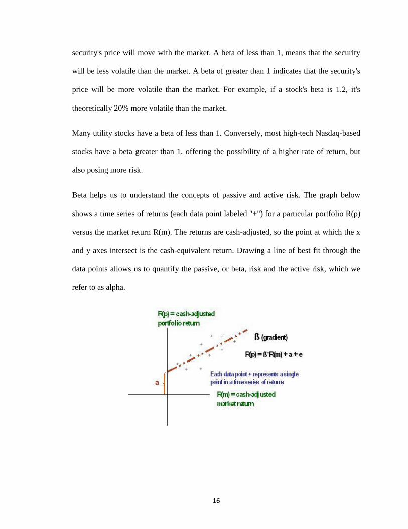
Beta helps us to understand the concepts of passive and active risk. The graph below

shows a time series of returns (each data point labeled "+") for a particular portfolio R(p)

versus the market return R(m). The returns are cash-adjusted, so the point at which the x

and y axes intersect is the cash-equivalent return. Drawing a line of best fit through the

data points allows us to quantify the passive, or beta, risk and the active risk, which we

refer to as alpha.

17

The gradient of the line is its beta. For example, a gradient of 1.0 indicates that for every

unit increase of market return, the portfolio return also increases by one unit. A manager

employing a passive management strategy can attempt to increase the portfolio return by

taking on more market risk (i.e., a beta greater than 1) or alternatively decrease portfolio

risk (and return) by reducing the portfolio beta below 1. Essentially, beta expresses the

fundamental tradeoff between minimizing risk and maximizing return. Let's give an

illustration. Say a company has a beta of 2. This means it is two times as volatile as the

overall market. Let's say we expect the market to provide a return of 10% on an

investment. We would expect the company to return 20%. On the other hand, if the

market were to decline and provide a return of -6%, investors in that company could

expect a return of -12% (a loss of 12%). If a stock had a beta of 0.5, we would expect it to

be half as volatile as the market: a market return of 10% would mean a 5% gain for the

company.

Investors expecting the market to be bullish may choose funds exhibiting high betas,

which increase investors' chances of beating the market. If an investor expects the market

to be bearish in the near future, the funds that have betas less than 1 are a good choice

because they would be expected to decline less in value than the index. For example, if a

fund had a beta of 0.5 and the S&P 500 declined 6%, the fund would be expected to

decline only 3%.

2.3 Empirical Review

Various studies have been undertaken both locally and internationally to explore the

profile relationship of quoted firms. Kamau (2002) reviews the profile relationship of

18

firms quoted on the Main Investment Market Segment (MIMS) and the Alternative

Investment Market Segment (AIMS). The study utilized historical market data from the

NSE for the period between January 1996 and December 2000. Individual firms Sharpe

Ratios fort the entire period were computed and analyzed. Differences between Sharpe

Ratios of firms listed under the MIMS and those of firms listed under AIMS were

analyzed using Wilcoxon Rank Sum Test. The research found out that there was no

significant difference in terms of return and risk between those firms listed under the

MIMS and AIMS.

Gitari (1990) established that quoted firms in Kenya display a positive relationship

between risk and return. The relationship was however not significant hence implying

investors may end up being under or over compensated for taking high risks.

Munywoki(1998) in a study conducted at the NSE to estimate systematic risk

approximated the systematic risk to be at 3.5% and market returns to be 14.8%. The study

also estimated the NSE beta to be 0.9002 attributing the difference between his estimated

beta and the beta of 1.0 to sampling. Ombajo (2006) carried out a study to determine the

extent to which NSE market segmentation affected the share prices of listed firms,

liquidity and investor recognition. The event study methodology pioneered by Fama et al.

(1969) was employed in carrying out the study. The study focused on the MIMS and the

AIMS.

Akwimbi (2003) studied the NSE on the application of APT for predicting stock returns

concluded that APT model had more success in explaining the expected return on the

NSE and asserted that the APT model holds true for emerging markets. Gichana (2009)

19

in his empirical study on linear and non-linear models deduced that non-linear models are

better than linear ones in predicting stock returns. Gichana’s findings further emphasized

that stock returns in this market is non-linear with risk.

The results of the study did not support Jacque (2004) assertion that segmentation is a

form of financial innovation which could lead to efficiency and thus a reduction in the

cost of capital without commensurate increase in systematic risk. No new listings were

seen during the period of study after segmentation of the market implying that

segmentation did not have an immediate impact on the cost of capital. The same result on

the NSE was also found to be true by Nkonge(2010) and Mogunde(2011) who both

concluded that profile is a factor of several functions. Kiptoo (2010) had earlier attributed

this to selected macroeconomic variables and stock prices.

International studies on industry dynamics in stock studies have also been reviewed.

Some of the most important findings of Sharpe-Lintner-Black model are anomalies. The

empirical attack on this model has begun with the studies that have identified variables

other than market β to explain cross-section of expected returns. Basu (1977) have

showed that earning-to-price ratio have marginal explanatory power after controlling for

β, expected returns are positively related to E/P. Banz (1981) has found that a stock size

(price times share) could help explain expected returns, given these market β, expected

returns on small stocks are too high and expected returns on large stocks are too low.

Bhandari (1988) has explored that leverage is positively related to expected stock returns,

Fama and French (1992) have found that higher book-to-market ratios are associated with

higher expected return, in their tests that also include market β.

20

These anomalies are now stylized facts to be explained by multifactor asset pricing

models of Merton (1973) and Ross (1976). For example Ball (1978) have argued that E/P

is a catch-all proxy for omitted factors in asset pricing tests and one can expect it to have

explanatory power when asset pricing follow a multifactor model and all relevant factors

are not included. Chan and Chen (1991) have argued that size effect is due to the fact that

small stocks include many martingale or depressed firms whose performance is sensitive

to business conditions. Fama and French (1992) have shown that since leverage and

book-to-market equity are also largely driven by market value of equity, they also may

proxy for risk factors; in return that are related to market judgments about the relative

prospects of firms. One can expect when asset pricing follow a multifactor models and all

relevant factors included in the asset pricing tests to explain these anomalies. There are

some other research works, which have shown that there is indeed spillover effect among

Sharpe-Lintner anomalies. Basu (1983) have found that size and E/P are related; Fama

and French (1992) have found that size and book to market equity are related and again

leverage and book in market equity are highly correlated.

These multifactor asset pricing models generalize the result of SLB model. In these

models, the return generating models involve multiple factors and the cross section of

expected returns is explained by the cross section of factor loadings or sensitivities. One

approach suggested by Ross (1976) arbitrage pricing theory (APT) uses factor analysis to

extract the common factors and then tests whether expected returns are explained by the

cross section of the loading of asset returns on the factor [Roll and Ross (1980); Chen

(1983); Lehmann and Modest (1988)] have tested this approach in detail. The factor

analysis approach to test of the APT leads to unreasonable conflict about the number of

21

common factors and what these factors are. The factor analysis approach is limited, but it

confirms that there is more than one common factor in explaining expected returns.

Now as regards the empirical testing of selected stock exchanges, Green (1990) have

tested CAPM on UK private sectors data and found that SLB model do not hold. But

Sauer and Murphy (1992) have investigated this model in German stock market data and

confirmed CAPM as the best model describing stock returns. Contradictory evidence has

been found by Hawawini(1993) in equity markets in Belgium, Canada, France, Japan,

Spain, UK and USA. The other studies, which tested CAPM for emerging markets are

Lau et al. (1975) for Tokyo Stock Exchange, Sareewiwathana and Malone (1985) for

Thailand stock exchange, Bark (1991) for Korean Stock Exchange and Gupta and Sehgal

(1993) for Indian stock Exchange. Badar (1997) has estimated CAPM for Pakistan.

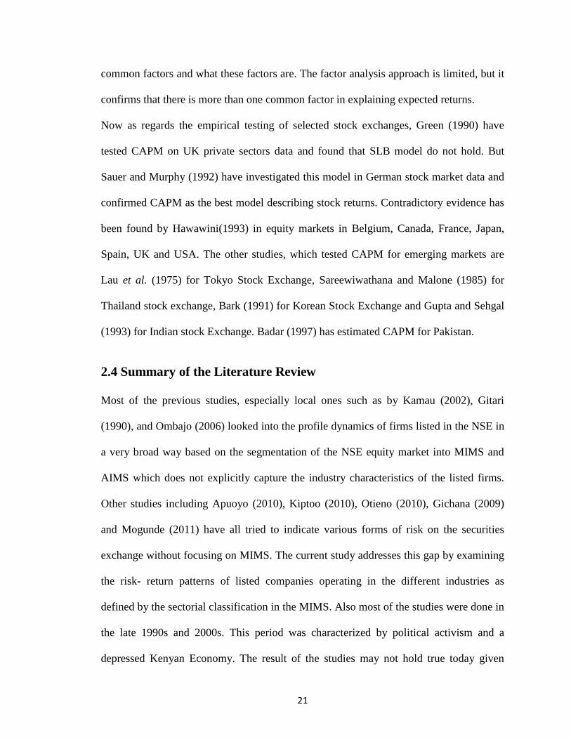
2.4 Summary of the Literature Review

Most of the previous studies, especially local ones such as by Kamau (2002), Gitari

(1990), and Ombajo (2006) looked into the profile dynamics of firms listed in the NSE in

a very broad way based on the segmentation of the NSE equity market into MIMS and

AIMS which does not explicitly capture the industry characteristics of the listed firms.

Other studies including Apuoyo (2010), Kiptoo (2010), Otieno (2010), Gichana (2009)

and Mogunde (2011) have all tried to indicate various forms of risk on the securities

exchange without focusing on MIMS. The current study addresses this gap by examining

the risk- return patterns of listed companies operating in the different industries as

defined by the sectorial classification in the MIMS. Also most of the studies were done in

the late 1990s and 2000s. This period was characterized by political activism and a

depressed Kenyan Economy. The result of the studies may not hold true today given

22

positive changes in the economic environments as well as the relative political maturity

that the country has lately achieved. In addition, the trading systems, such as the open

outcry system, that was in operation during the time of the previous studies were largely

manual. This could have affected the efficiency of operations, the flow of information as

well as pricing of assets, all of which affect stock returns replaced by adoption of the

Automated Trading System (ATS) in 2005 and the full implementation of the Central

Depository and Settlement System (CDSS) in 2006. The current study therefore seeks to

understand whether the results of previous studies still hold in the improved trading

environment in the period 2009-2012 using a CAPM model to support or contradict the

scholars mentioned.

23

CHAPTER THREE: RESEARCH METHODOLOGY

3.1 Introduction

Chapter three focuses on the methodology of the study. It identifies the research design,

the population of study, the sample, the sampling technique, data collection and source. It

further explains the measurement and operationalization of variables to be used and

finally the analysis of data to be collected.

3.2 Research Design

This study is quantitative and explanatory and uses available data to investigate

correlations and examine regressions among variables. Therefore the research design in

this study is casual comparative. The reason for this design is that the independent

variables of the study cannot be manipulated experimentally and thus it is not possible to

investigate the relationship between dependent and independent variables through

experimental design.

3.3 Population of Study

The target population of study was all listed companies operating in Kenya under the

MIMS division. The source of this population was the Nairobi Securities Exchange

where a list of thirty quoted companies was obtained as at 31st December 2012. This date

was identified as the cut-off date for the purpose of carrying out this study.

3.4 Sampling

A sample of thirty listed firms was selected to form the sample for this study analysis

after surveying the listed firms as at 2009 using Wednesday averages as recommended by

24

Fama and French (1983). These thirty firms were those that are constantly active in the

market.

3.5 Data Collection

This study used average monthly stocks returns from 30 companies listed on the NSE for

the period of 4years. The stocks were the most active on the NSE and their data was

obtained from the NSE offices in the form of daily prices. The data used was therefore

purely secondary data purchased from NSE.

This study used the average monthly prices for a stock to represent monthly data and

NSE 20 share index as the proxy of the market index. The index is a valued weighted

index comprising of 20 most traded stocks and reflects the trend of the market. The

existing 91days Treasury bill was used as a proxy for the risk free rate. All stock returns

used for the purpose of this paper were not adjusted for dividends.

3.6 Data Analysis

To test the CAPM for the Nairobi securities exchange, a four year period was used as

well as methods introduced by Black et.al (1972) and Fema-MacBeth (1973). The

investigation is divided into three main periods. These are the portfolio formation period,

estimation period, and testing period.

3.6.1 Portfolio Formation Period

The portfolio formation period is the first step of the test. The study used this period to

estimate beta coefficient for individual stocks using average monthly returns for the four

year period. The estimation was conducted by regression using the following time series

formula:

25

Rit – Rft = ai + βi(Rmt – Rft) + eit……………………………………(1)

Where

Rit = rate of return on stock i (i = 1 . . . 30)

Rft = risk free rate at time t

βi = estimate of beta for stock i

Rmt = rate of return on the market index at time t

eit = random disturbance term in the regression equation at time t

The above equation is also expressible as

rit = ai + βi.rmt+eit

Where

rit = Rit – Rft = excess return of stock i (i = 1 . . . 30)

rmt = Rmt – Rft = average risk premium.

ai = the intercept.

The intercept ai is supposed to be the difference between estimated return produced by

time series and the expected return predicted by CAPM. The intercept ai of a stock is

equivalent to zero if CAPM’s description of expected return is accurate. The individual

stock’s beta once obtained after series of estimation are used to create equally weighted

average portfolios. The equally weighted average portfolios are created according to

high-low beta criteria. Portfolio one contains a set of securities with the highest betas

while the last portfolio contains a set of low beta securities. Organizing and grouping

securities into portfolios is considered a strategy of partially diversifying away a portion

of risk whereby increasing the chances of a better estimation of beta and expected return

of the portfolio containing the securities.

26

3.6.2 Initial Estimation Period

Within this estimation period, regression is run using the beta information obtained from

the previous period. The purpose of this period is to estimate individual portfolio betas.

Fama- MacBeth applied crossed-sectional regression on its data and regress average

excess return on market beta of portfolios. The formula used to calculate portfolios’ beta

is;

rpt = ap + βp.rmt+ ept………………………………….(2)

Where

rp = average excess portfolio return

βp= portfolio beta

3.6.3Testing Period

After estimating the portfolios’ betas in the previous period, the next step is estimating

the ex-post Security Market Line (SML) by regressing the portfolio returns against

portfolio betas. To estimate the ex-post Security Market Line, the following equation is

examined:

rp = y0 + y1βp+ ep…………………………………………………(3)

Where

rp = average excess portfolio return

βp = estimate of beta portfolio p

y0 = zero-beta rate

y1 = market price of risk and

ep = random disturbance term in the regression equation

27

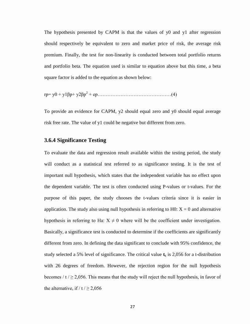
The hypothesis presented by CAPM is that the values of y0 and y1 after regression

should respectively be equivalent to zero and market price of risk, the average risk

premium. Finally, the test for non-linearity is conducted between total portfolio returns

and portfolio beta. The equation used is similar to equation above but this time, a beta

square factor is added to the equation as shown below:

rp= y0 + y1βp+ y2βp2 + ep………………………………………(4)

To provide an evidence for CAPM, y2 should equal zero and y0 should equal average

risk free rate. The value of y1 could be negative but different from zero.

3.6.4 Significance Testing

To evaluate the data and regression result available within the testing period, the study

will conduct as a statistical test referred to as significance testing. It is the test of

important null hypothesis, which states that the independent variable has no effect upon

the dependent variable. The test is often conducted using P-values or t-values. For the

purpose of this paper, the study chooses the t-values criteria since it is easier in

application. The study also using null hypothesis in referring to H0: X = 0 and alternative

hypothesis in referring to Ha: X ≠ 0 where will be the coefficient under investigation.

Basically, a significance test is conducted to determine if the coefficients are significantly

different from zero. In defining the data significant to conclude with 95% confidence, the

study selected a 5% level of significance. The critical value tc is 2,056 for a t-distribution

with 26 degrees of freedom. However, the rejection region for the null hypothesis

becomes / t / ≥ 2,056. This means that the study will reject the null hypothesis, in favor of

the alternative, if / t / ≥ 2,056

28

CHAPTER FOUR: DATA ANALYSIS, RESULTS AND DISCUSSION

4.1 Introduction

In this part, results obtained from the application of the empirical methods discussed in

the previous chapter are presented. The methods are the basis for the test of CAPM.

Equally, analysis of the results obtained will be made within this section

4.2 Portfolio Formation

At this initial stage, beta values of the individual stocks are estimated using equation (1).

A detailed table containing stocks, betas and their average access returns is included in

appendix

4.2.1 Initial Estimation

With a condition that the relationship between stocks and betas is established, the next

stage is to form portfolios using the sizes of the individual betas. Using this information,

three portfolios were formed each consisting of ten stocks and regressed using equation 2.

The individual portfolio beta estimate along with its average access return is given in

table one

Portfolio no Portfolio beta Average excess return

1 1.2012 -0.0304

2 1.1510 -0.0131

3 0.9122 0.0739

Table one. Portfolio beta estimates

29

4.2.2 Testing

The SML coefficients are estimated using equation (3) since the values of the portfolio

betas are known. The results are summarized in the table below;

Coefficients Std. Error t-statistic probability

Y0 0.2415 0.07300 2.9684 0.0428

Y1 -0.1387 0.6141 -2.0533 0.1139

Table two. Statistic SML estimation

The last step is to test for non-linearity between average excess portfolio returns and

betas. To do this, equation (4) is used in regression using a beta square factor. The result

is summarized below;

Coefficients Std. Error t-statistic Probability

Y0 0.2859 0.3815 0.6947 0.6133

Y1 -0.2518 0.5413 -0.3815 0.8042

Y2 0.04013 0.2135 0.2243 0.9215

Table three. Statistic for non-linearity test

4.3 Discussions and Interpretations of Findings

The result in table one containing portfolio betas and their average excess returns,

presents the nature of high beta/ high return and low beta/low return criteria described by

the CAPM. The characteristics of the result do not provide support of the hypothesis.

That is, portfolio one with the highest beta does not have a high return in comparison to

portfolio three, which has a lower beta but is associated with the highest return amongst

all the portfolios. To support the theory, returns on portfolios should match their betas.

Table two shows statistic SML estimation, the hypothesis presented by CAPM is that the

values of y0 and y1 after regression should respectively be equivalent to zero and market

30

price of risk, the average risk premium. The null hypothesis that the intercept y0 is zero,

is rejected at 5% level of significance since the t-value is larger than 2.056. This actually

means that the coefficient is significantly different from zero, which is a contradiction to

the theory of CAPM.

Conducting a test for the second coefficient y1 indicates that the value of the coefficient

is significantly different from zero at 5% significance level since its t-value is larger than

2.056.The calculated value is 0.00213 while the estimated value is –0.1387, which

appears to be a contradiction to CAPM.

To provide an evidence for CAPM, y2 should equal zero and y0 should equal average risk

free rate. The value of y1 must equal the average risk premium. The nature of y2 shall

determine the linearity condition between risk and return. The test indicates that the value

of the intercept y0is not significantly different from zero since its t-value is greater than

2.056. However, this value is not equal to the average risk free rate, 0.05385 and is thus

evidence against CAPM.

Though the coefficient of y1 is negative as per table three, the test indicates that it is also

not significantly different from zero since its absolute t-value is smaller than 2.056. As

well, the coefficient is not equal to the average market premium as described by CAPM.

The test conducted for y2 indicates that the coefficient is not significantly different from

zero and provides an evidence for CAPM. Well, having the coefficient not significantly

different from zero signifies that the expected rate of returns and betas are linearly related

to each other.

31

CHAPTER FIVE: SUMMARY, CONCLUSION AND

RECOMMENDATIONS

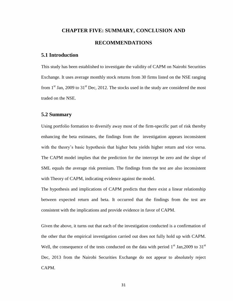
5.1 Introduction

This study has been established to investigate the validity of CAPM on Nairobi Securities

Exchange. It uses average monthly stock returns from 30 firms listed on the NSE ranging

from 1st Jan, 2009 to 31

st Dec, 2012. The stocks used in the study are considered the most

traded on the NSE.

5.2 Summary

Using portfolio formation to diversify away most of the firm-specific part of risk thereby

enhancing the beta estimates, the findings from the investigation appears inconsistent

with the theory’s basic hypothesis that higher beta yields higher return and vice versa.

The CAPM model implies that the prediction for the intercept be zero and the slope of

SML equals the average risk premium. The findings from the test are also inconsistent

with Theory of CAPM, indicating evidence against the model.

The hypothesis and implications of CAPM predicts that there exist a linear relationship

between expected return and beta. It occurred that the findings from the test are

consistent with the implications and provide evidence in favor of CAPM.

Given the above, it turns out that each of the investigation conducted is a confirmation of

the other that the empirical investigation carried out does not fully hold up with CAPM.

Well, the consequence of the tests conducted on the data with period 1st Jan,2009 to 31

st

Dec, 2013 from the Nairobi Securities Exchange do not appear to absolutely reject

CAPM.

32

There are some procedures which could improve upon this study and bring further depth

to this experiment. While compiling any portfolio, diversification is always a necessary

precaution. Complete diversification among stocks in any given portfolio is difficult to

obtain, and in this study it is possible that our portfolios were not as diversified as they

could have been. Therefore, to expand upon this study, it would be beneficial to ensure

that much diversified stocks were collected.

Also, this study only used publicly traded stocks to be the component of a portfolio

instead of using bonds, real estate, foreign exchange, or a hybrid of the above. With a

hybrid of investments, it is possible to expose different results and provide more insights

for the validity of using CAPM in approximating expected return with beta risk.

5.3 Conclusions

The basic aim of this study was to check the applicability of CAPM to NSE, whether it

gives accurate results. After the analysis of thirty different companies listed on NSE, for

the period of four years (2009-2012), it was found that the Capital Asset Pricing Model,

failed to give accurate results. Though very slight evidence was seen, regarding the

applicability of CAPM, but it was only in traces. These findings help in concluding that

CAPM is not fully applicable to the NSE. A strong rejection has been seen, regarding the

acceptance and applicability of CAPM (Levy, 1997). Even though significant evidence

has been put forward against the use of CAPM, still it remains a good tool for finding out

the cost of capital, investment performance evaluation, and studies of efficient market

events (Moyer et al, 2001; Campbell et al, 1997). CAPM has provided knowledge, about

the capital market and market conditions (Karnosky, 1993).

33

In short, CAPM is not an effective model to measure risk and required return, and

investors, therefore may not depend or rely on it in their investment decisions.

5.4 Limitations of the Study

I cannot state that the data do not support CAPM since there are other factors available

and capable of affecting the results such as measurement and model specification errors.

These errors, however, arises because of the usage of a proxy and not the real market

portfolio and leads to biasing the estimated slope towards zero as well as estimating the

intercept away from zero.

This project has only evaluated CAPM in combination with historical data of stocks

obtained from Nairobi Securities Exchange. This study does not present an evidence for

any other model even though it may present inconsistency with CAPM.

The results confirmed that the standard CAPM is not verified in the NSE during the

period of study. The evidence discussed above does not prove that the CAPM is invalid

since only stocks were included in the analyses. The market portfolio contains all of the

capital assets. We will never be able to observe the returns on the “true” market portfolio.

Therefore, the CAPM is simply not a testable theory. The estimated betas are very

sensitive to the market index being used. In risk-return space, indices can be close to each

other and close to the efficient set, and still produce different relationships (positive and

negative) between return and beta.

It is important to know that the main reason that we test the CAPM is to analyze the

relation between the risk and return of the securities and - in our case - the risk and return

of the portfolios. The testable implications of the CAPM show that all investors hold

34

risky assets in the same proportion and, in particular, every investor hold the same

proportion of stocks. In order to achieve the desired balance of risk and return, investors

simply vary the fraction of their portfolios made up of the riskless assets.

5.5 Recommendations

There is need to understand that there were enough drawbacks during the data analysis.

And the results showed that the CAPM is rejected in the Nairobi Securities Exchange.

That is why more empirical tests on the NSE should be applied, using alternative

financial models. In my opinion, a test on the NSE using the APT model, would give

more complete results, as it could include different variables like the inflation rate and the

market value of securities. Thus, further researches and more tests on the APT should be

applied, in order for the researchers, the managers of firms and investors - to have more

accurate results and understand the risk-return trade off of the NSE securities. Another

project would be to release other assumptions and to tests the models based on different

hypotheses. In this way we might have results that would lead to new theories on asset

pricing models.

5.5.1 Suggestions for further Research

Future studies, may consider a detailed comparison of results from CAPM for NSE, and

other stock markets of developing and developed states. These studies may also consider

the use of more sophisticated tools (i.e. GARCH), and models like the multifactor

models, Arbitrage Pricing Theory (APT). It is suggested that in future studies, CAPM

should be tested individually and along with the multi-factor model (APT), for the better

understanding of the risk/return relationship and pricing mechanisms.

35

REFERENCES

Akwimbi, W. (2003). Application of APT in predicting stock returns at the Nairobi Stock

Exchange. Unpublished MBA Project, University of Nairobi.

Apuoyo, B. (2010). Relationship between Working Capital Management Policies and

Profitability for Companies Quoted at the NSE. Unpublished MBA Project,

University of Nairobi.

Gichana, I. (2009). Comparison of Linear and Non-Linear Models in Predicting Stock

Returns at the Nairobi Stocks Exchange. Unpublished MBA Project, University of

Nairobi.

Kamau, G. (2002). An Investigation into the Relationship between Risk and Return of

Companies Listed Under the various Market Segments; the Case of the NSE.

Unpublished MBA project, University of Nairobi.

Kiptoo, S. (2010). An Empirical Investigation of the Relationship between Selected

Macro-Economics Variables and Stock Prices. Unpublished MBA Project,

University of Nairobi.

Nkonge, T. (2010). Effects of Stock Splits on Security Returns of firms Listed on the

NSE. Unpublished MBA Project,University of Nairobi.

Ombajo, N. (2006). Share Price Reaction to Stock Market Segmentation of NSE.

Unpublished MBA Project,University of Nairobi.

Omogo, B. (2011). Risk-Return Trade- Off for Companies Quoted on the Nairobi

Securities Exchange. Unpublished MBA Project,University of Nairobi.

36

Ondari, M. (2012). Risk-Return Profile for Companies Quoted at the Nairobi Securities

Exchange. Unpublished MBA Project,University of Nairobi.

Cooper, M. G. (2008). Asset Growth and Crossection of Stock Returns. Journal of

Finance,Vol.63, 1609-51.

Da, Z. (2009). Cash Flow, Consumption Risk, and Crossection of Stocks Returns.

Journal of Finance,Vol.64, 923-56.

Daniel, K. A. (1997). Evidence on the Characteristics of Crosssectional Variation in

Stock Returns . Journal of Finance, Vol. 53, 1-33.

F., B. (1973). Beta and Return. Journal of Portfolio Manangement, Vol 20.

Fama, E. A. (1973). Risk Return and Equilibrium: Empirical Tests. . Journal of Political

Economy, Vol 81.

Fama, E. A. (1992). The Cross Section of Expected Stock Returns. Journal of Finance

Vol. 47, 427-466.

Fama, E. A. (1993). Common Risk Factors in the Returns on Stocks and Bonds . Journal

of Financial Economics Vol.33, 3-56.

Fama, E. A. (1995). Industry Cost of Equity. Working Paper, Graduate School of

Business,University of Chicago Vol. 50, 3-25.

Fama, E. A. (2004). The Capital Asset Pricing Model:Theory and Evidence. The Journal

of Economic Perspectives, Vol. 18.

Fama, E. A. (2008). Dissecting Anomalies . Journal of Finance Vol. 63, 1653-78.

37

Graffin, J. A. (2002). Book to Market Equity, Distress Risk, and Stock Returns. Journal

of Finance, Vol.57, 2317-36.

Graffin, J. S. (2003). Momentum Investing and Business Cycle Risk:Evidence from Pole

to Pole. Journal of Finance Vol.58, 2515-47.

Grinblatt, M. A. (2004). Predicting Stock Price Movements from Past Returns:The Role

of Consistency and Tax-Loss Selling. Journal of Financial Economics, Vol.71,

541-79.

Heston, S. A. (2008). Seasonality in the Cross-Section of Stock Returns. Journal of

Financial Economics Vol. 87, 418-45.

Hong, H. L. (2000). Bad News Travels Slowly:Size,AnalystCoverage, and the

Profitability of Momentum Strategiee. Journal of Finance,Vol.55, 265-95.

i

APPENDIX I: LISTED COMPANIES AT NSE Agricultural

Symbol Listing Notes

EGAD Eaagads Limited Coffee growing and sales

KAZU Kakuzi Limited Coffee, tea, passionfruit, avocados, citrus, pineapple,

others

KAPC Kapchorua Tea Company Limited Tea growing, processing and marketing

LIMR Limuru Tea Company Limited Tea growing

RVP Rea Vipingo Sisal Estate Sisal

STC Sasini Tea and Coffee Tea, coffee

GWKL Williamson Tea Kenya Limited Tea growing, processing and distribution

Automobiles and Accessories

Symbol Listing Notes

CARG Car & General Kenya Automobiles, engineering, agriculture

CMC CMC Holdings Automobile distribution

MSHA Marshalls East Africa Automobile assembly

FEAL Sameer Africa Limited Tires

Banking

Symbol Listing Notes

BARC Barclays Bank (Kenya) Banking, finance

CFCO CFC Stanbic Holdings Banking, finance

DTK Diamond Trust Bank

Group Banking, finance

EQTY Equity Bank Group Banking, finance; crosslisted at the Uganda Securities Exchange

HOUS Housing Finance

Company of Kenya Mortgage financing

ii

KCBK Kenya Commercial

Bank Group

Banking & finance. Crosslisted on the Uganda Securities Exchange, the

Dar es Salaam Stock Exchange and the Rwanda Over The Counter

Exchange

NABK National Bank of Kenya Banking, finance

NINC National Industrial

Credit Bank Banking, finance

SCBK Standard Chartered

Kenya Banking, finance

COOP Cooperative Bank of

Kenya Banking, finance

Commercial and Services

Symbol Listing Notes

EXPK Express Kenya Limited Logistics

HBL Hutchings Biemer Limited Furniture

KAL Kenya Airways Kenya's flagship airline; crosslisted at Uganda Securities

Exchange and Dar es Salaam Stock Exchange

LKL Longhorn Kenya Limited Publishing

NMG Nation Media Group Newspapers, magazines, radio stations, television stations

SCAN Scangroup Advertising and marketing

STDN Standard Group Limited Publishing

TPS TPS Serena Hotels &resorts

UCHU Uchumi Supermarkets Supermarkets

Construction and Allied

Symbol Listing Notes

ARM Athi River Mining Limited Cement, fertilizers, minerals; mining and manufacturing

BAMB Bamburi Cement Limited Cement

CRWN Crown-Berger (Kenya) Paint manufacturing

iii

CABL East African Cables Limited Cable manufacture

EAPC East African Portland Cement

Company Cement manufacture and marketing

Energy and Petroleum

Symbol Listing Notes

KGEN Kengen Electricity generation

KOCL KenolKobil Petroleum importation, refining, storage & distribution

KPLA Kenya Power and Lighting

Company Electricity transmission, distribution and retail sale

TOPL Total Kenya Limited Petroleum importation and distribution

UMEME Umeme Electric power distribution. Crosslisting from Uganda

Securities Exchange[1]

Insurance

Symbol Listing Notes

BAI British-American Investments Co.(Kenya) Insurance

CIHL Liberty Kenya Holdings Limited (formally

CFC Insurance) Insurance

JHL Jubilee Holdings Limited Insurance, investments; crosslisted at the Uganda

Securities Exchange

KRIN Kenya Re-Insurance Corporation Reinsurance

PAIC Pan Africa Insurance Holdings Insurance

Investment

Symbol Listing Notes

CENTUM Centum Investment Company Investments

CITY[2]

City Trust[3]

Financial services

OLYM Olympia Capital Holdings Construction and building materials

TRCY TransCentury Investments Investments

iv

Manufacturing and Allied

Symbol Listing Notes

BAUM A Baumann and Company Machinery distribution and marketing, investments

BOC BOC Kenya Industrial gases, welding products

BAT British American Tobacco

Limited Tobacco products

CARB Carbacid Investments Limited Carbon dioxide manufacturing

EABL East African Breweries Beer, spirits; crosslisted at Uganda Securities Exchange and Dar

es Salaam Stock Exchange

EVRD Eveready East Africa batteries

KOL Kenya Orchards Limited Fruit growing, preservation and distribution, fruit-juice

manufacture and marketing

MSCL Mumias Sugar Company

Limited Sugar cane growing, sugar manufacture & marketing

UNGA Unga Group Flour milling

Telecommunication and Technology

Symbol Listing Notes

ACES Access Kenya Group Internet service provider

SCOM Safaricom Mobile telephony

v

APPENDIX I: A list of sample firms Betas and Excess return

Number Stock Beta

Excess

Return

1 Crown Berger Ltd 0rd 5.00 1.137 0.3887

2 Scangroup Ltd Ord 1.00 1.255 0.8997

3 Barclays Bank Ltd Ord 2.00 1.029 -0.7837

4 E.A.Portland Cement Ltd Ord 5.00 1.116 -0.4247

5 East African Breweries Ltd Ord 2.00 1.224 0.4618

6 KenGen Ltd. Ord. 2.50 1.097 0.1078

7 Sasini Ltd Ord 1.00 1.249 1.2441

8 Sameer Africa Ltd Ord 5.00 1.227 0.0653

9 Total Kenya Ltd Ord 5.00 1.093 -0.6967

10 Kenya Power & Lighting Ltd Ord 20.00 1.061 -0.2276

11

Diamond Trust Bank Kenya Ltd Ord

4.00 0.787 0.5423

12 National Bank of Kenya Ltd Ord 5.00 1.0054 -0.4847

13 Equity Bank Ltd Ord 5.00 1.028 -0.0467

14 Housing Finance Co Ltd Ord 5.00 0.1045 0.5192

15 Jubilee Holdings Ltd Ord 5.00 0.1797 0.2225

16 NIC Bank Ltd 0rd 5.00 -0.034 -0.4527

17 Standard Chartered Bank Ltd Ord 5.00 1.002 0.0102

18

The Co-operative Bank of Kenya Ltd

Ord 1.00 0.912 0.4036

19 Safaricom limited Ord 0.05 0.951 0.4460

20

TPS Eastern Africa (Serena) Ltd Ord

1.00 0.943 1.2325

21 Rea Vipingo Plantations Ltd Ord 5.00 0.831 1.4258

22 AccessKenya Group Ltd Ord. 1.00 0.116 0.4920

23 Kenya Airways Ltd Ord 5.00 0.245 -0.4870

24 Nation Media Group Ord. 2.50 0.877 -0.3452

25 Kenya Commercial Bank Ltd Ord 1.00 0.803 0.6833

26 CFC Stanbic Holdings Ltd ord.5.00 0.617 -0.3257

27

British American Tobacco Kenya Ltd

Ord 10.00 0.562 -0.2387

28 E.A.Cables Ltd Ord 0.50 0.563 -0.4997

29 Kenya Oil Co Ltd Ord 0.50 0.892 -0.0141

30 Athi River Mining Ord 5.00 0.907 0.9870